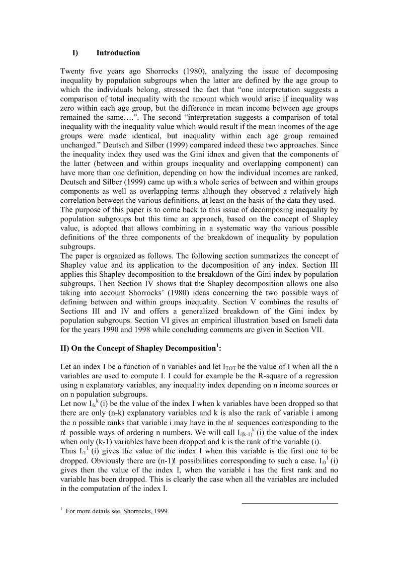
On the Shapley Value and the Decomposition of Inequality by Population Subgroups

with Special Emphasis on the Gini Index

by

Joseph Deutsch*

and

Jacques Silber*

• Department of Economics, Bar-Ilan University, 52900 Ramat-Gan, Israel.

March 2005

Not to be quoted without the authors’ permission

1

Key Words: Decomposition – Gini Index – Groups - Inequality - Israel – Overlapping - Shapley Value

Abstract

This paper proposes a generalization of the breakdown of income inequality by population subgroups that is based on the idea that either the within or the between groups inequality should be considered as a residual. This generalization of the inequality decomposition uses the concept of Shapley value and is applied to the Gini index which assumes that the ranking of individuals plays also a role. The paper includes an empirical illustration using Israeli Income data for the years 1990 and 1998.

2

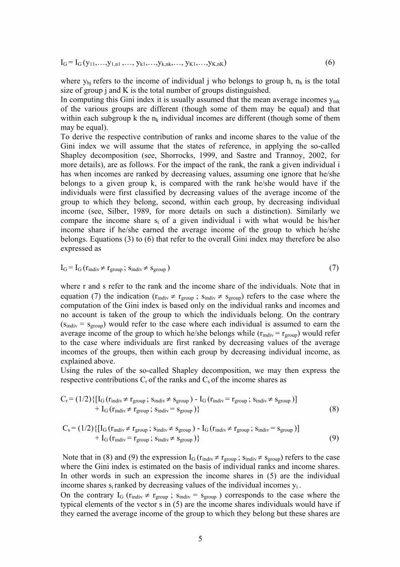
I) Introduction Twenty five years ago Shorrocks (1980), analyzing the issue of decomposing inequality by population subgroups when the latter are defined by the age group to which the individuals belong, stressed the fact that “one interpretation suggests a comparison of total inequality with the amount which would arise if inequality was zero within each age group, but the difference in mean income between age groups remained the same….”. The second “interpretation suggests a comparison of total inequality with the inequality value which would result if the mean incomes of the age groups were made identical, but inequality within each age group remained unchanged.” Deutsch and Silber (1999) compared indeed these two approaches. Since the inequality index they used was the Gini idnex and given that the components of the latter (between and within groups inequality and overlapping component) can have more than one definition, depending on how the individual incomes are ranked, Deutsch and Silber (1999) came up with a whole series of between and within groups components as well as overlapping terms although they observed a relatively high correlation between the various definitions, at least on the basis of the data they used. The purpose of this paper is to come back to this issue of decomposing inequality by population subgroups but this time an approach, based on the concept of Shapley value, is adopted that allows combining in a systematic way the various possible definitions of the three components of the breakdown of inequality by population subgroups. The paper is organized as follows. The following section summarizes the concept of Shapley value and its application to the decomposition of any index. Section III applies this Shapley decomposition to the breakdown of the Gini index by population subgroups. Then Section IV shows that the Shapley decomposition allows one also taking into account Shorrocks’ (1980) ideas concerning the two possible ways of defining between and within groups inequality. Section V combines the results of Sections III and IV and offers a generalized breakdown of the Gini index by population subgroups. Section VI gives an empirical illustration based on Israeli data for the years 1990 and 1998 while concluding comments are given in Section VII.

II) On the Concept of Shapley Decomposition1: Let an index I be a function of n variables and let ITOT be the value of I when all the n variables are used to compute I. I could for example be the R-square of a regression using n explanatory variables, any inequality index depending on n income sources or on n population subgroups. Let now I/k

k (i) be the value of the index I when k variables have been dropped so that there are only (n-k) explanatory variables and k is also the rank of variable i among the n possible ranks that variable i may have in the n! sequences corresponding to the n! possible ways of ordering n numbers. We will call I/(k-1)

k (i) the value of the index when only (k-1) variables have been dropped and k is the rank of the variable (i). Thus I/1

1 (i) gives the value of the index I when this variable is the first one to be dropped. Obviously there are (n-1)! possibilities corresponding to such a case. I/0

1 (i) gives then the value of the index I, when the variable i has the first rank and no variable has been dropped. This is clearly the case when all the variables are included in the computation of the index I.

1 For more details see, Shorrocks, 1999.

Similarly I/22 (i) corresponds to the (n-1)! cases where the variable i is the second one

to be dropped and two variables as a whole have been dropped. Clearly I/22 (i) can also

take (n-1)! possible values. I/12 (i) gives then the value of the index I, assuming only

one variable was eliminated and the variable i has the second rank. Here also there are (n-1)! possible cases. Obviously I/(n-1)

n (i) corresponds to the (n-1)! cases where the variable i is dropped last and is the only one to be taken into account. If I is an inequality index, it will evidently be equal to zero in such a case. But if it is for example the R-square of a regression it would give us the R-square when there is only one explanatory variable, the variable i. Obviously I/n

n (i) gives the value of the index I when variable i has rank n and n variables have been dropped, a case where I will always be equal to zero by definition since no variable is left. Let us now compute the contribution Cj(i) of variable i to the index I, assuming this variable i is dropped when it has rank j. Using the previous notations we define Cj(i) as Cj(i) = (1/n!) ∑h=1 to (n-1)! [I/(j-1)

j (i) - I/jj (i)]h (1)

where the superscript h referes to one of the (n-1)! cases where the variable i has rank j. The overall contribution of variable i to the index I may then be defined as C(i) = (1/n!) ∑k=1 to n Ck(i) (2) It is then easy to prove that

I = (1/n!) ∑i=1 to n C(i) (3)

III) The Shapley Decomposition and the Respective Contribution of Ranks and Income Shares in the Traditional Decomposition of the Gini Index Numerous definitions of the Gini index have appeared in the literature (see, Yitzhaki, 1998) among which some clearly emphasize the fact that ranks play a role in the definition of the Gini Index. Such an approach has, for example, been proposed by Berrebi and Silber (1987) who defined the Gini index IG as IG = ∑i=1 to n ((n-2i+1)/n)) si (4) where si is the share of individual i who earns an income yi in the total income of the population, assuming that y1 ≥… yi ≥…≥ yn and n is the size of the population. Silber (1989) has however proven that equation (4) could be also expressed as IG = e’ G s (5) where e’ is a row vectors of individual population shares all equal to (1/n), s is a column vector of individual income shares ranked by decreasing income values yi while G is a square matrix called G-matrix whose typical element ghk is equal to 1 if h>k, to –1 if k>h and to 0 if h=k. Let us now assume that the population is divided into population subgroups. More precisely we will suppose that each individual i among the n individuals belongs to a subgroup k. Let now yki be the income of such an individual i who belongs to a subgroup k. Assuming there are nk individuals in each subgroup k, the overall Gini index IG may be expressed as a function

4

IG = IG (y11,…,y1,n1 ,…, yk1,…,yk,nk,…, yK1,…,yK,nK) (6) where yhj refers to the income of individual j who belongs to group h, nh is the total size of group j and K is the total number of groups distinguished. In computing this Gini index it is usually assumed that the mean average incomes ymk of the various groups are different (though some of them may be equal) and that within each subgroup k the nk individual incomes are different (though some of them may be equal). To derive the respective contribution of ranks and income shares to the value of the Gini index we will assume that the states of reference, in applying the so-called Shapley decomposition (see, Shorrocks, 1999, and Sastre and Trannoy, 2002, for more details), are as follows. For the impact of the rank, the rank a given individual i has when incomes are ranked by decreasing values, assuming one ignore that he/she belongs to a given group k, is compared with the rank he/she would have if the individuals were first classified by decreasing values of the average income of the group to which they belong, second, within each group, by decreasing individual income (see, Silber, 1989, for more details on such a distinction). Similarly we compare the income share si of a given individual i with what would be his/her income share if he/she earned the average income of the group to which he/she belongs. Equations (3) to (6) that refer to the overall Gini index may therefore be also expressed as IG = IG (rindiv ≠ rgroup ; sindiv ≠ sgroup ) (7) where r and s refer to the rank and the income share of the individuals. Note that in equation (7) the indication (rindiv ≠ rgroup ; sindiv ≠ sgroup) refers to the case where the computation of the Gini index is based only on the individual ranks and incomes and no account is taken of the group to which the individuals belong. On the contrary (sindiv = sgroup) would refer to the case where each individual is assumed to earn the average income of the group to which he/she belongs while (rindiv = rgroup) would refer to the case where individuals are first ranked by decreasing values of the average incomes of the groups, then within each group by decreasing individual income, as explained above. Using the rules of the so-called Shapley decomposition, we may then express the respective contributions Cr of the ranks and Cs of the income shares as Cr = (1/2){[IG (rindiv ≠ rgroup ; sindiv ≠ sgroup ) - IG (rindiv = rgroup ; sindiv ≠ sgroup )] + IG (rindiv ≠ rgroup ; sindiv = sgroup )} (8) Cs = (1/2){[IG (rindiv ≠ rgroup ; sindiv ≠ sgroup ) - IG (rindiv ≠ rgroup ; sindiv = sgroup )] + IG (rindiv = rgroup ; sindiv ≠ sgroup )} (9) Note that in (8) and (9) the expression IG (rindiv ≠ rgroup ; sindiv ≠ sgroup) refers to the case where the Gini index is estimated on the basis of individual ranks and income shares. In other words in such an expression the income shares in (5) are the individual income shares si ranked by decreasing values of the individual incomes yi . On the contrary IG (rindiv ≠ rgroup ; sindiv = sgroup ) corresponds to the case where the typical elements of the vector s in (5) are the income shares individuals would have if they earned the average income of the group to which they belong but these shares are

5

ranked by decreasing individual incomes. In other words the ranking of the individuals in computing IG (rindiv ≠ rgroup ; sindiv = sgroup ) is the same as that used in computing the regular Gini index IG (rindiv ≠ rgroup ; sindiv ≠ sgroup ). This index IG (rindiv ≠ rgroup ; sindiv = sgroup ) corresponds in fact to what Yitzhaki (1987) and Yitzhaki and Lerman (1991) have defined as the between groups Gini index (see, Deutsch and Silber, 1999) and which will be henceforth labelled as IBETWEEN YITZHAKI . Finally IG (rindiv = rgroup ; sindiv ≠ sgroup ) corresponds to the sum of the between and within groups Gini indices as they are usually estimated (see, Bhattacharya and Mahalanobis, 1967, and Silber, 1989), two expressions that will be henceforth labelled as IBETWEEN TRADITIONAL and IWITHIN TRADITIONAL. Here the income shares defining the vector s in (5) are given by the individual incomes yi and these shares si are ranked first by decreasing average incomes of the groups, second within each group by decreasing individual income (see, Silber, 1989). We may therefore write (8) and (9) also as Cr = (1/2){[IG,TOT – (IG,BETWEEN TRADITIONAL + IG,WITHIN TRADITIONAL)] + IG,BETWEEN YITZHAKI} (10) CS=(1/2){[IG,TOT–IG,BETWEEN YITZHAKI] + [IG,WITHIN TRADITIONAL+IG,BETWEEN TRADITIONAL]} (11) But [IG,TOT–(IG,BETWEEN TRADITIONAL+IG,WITHIN TRADITIONAL)] in (10) is by definition equal to the overlap IG, OVERLAP TRADITIONAL between the income distributions of the various groups (see, Deutsch and Silber, 1989) while [IG,TOT–IG,BETWEEN YITZHAKI] in (11) corresponds to Yitzhaki and Lerman’s (1991) within groups Gini Index denoted as IG,WITHIN YITZHAKI. We may therefore also express the contribution Cr of the ranks as Cr = (1/2) {IG,OVERLAP TRADITIONAL + IG,BETWEEN YITZHAKI } (12) Note that IG,BETWEEN YITZHAKI in expressions (11) to (12) reflects also the fact that there is overlap between the various income distributions. Similarly the contribution CS of the shares will be finally expressed as CS=(1/2){[IG,WITHIN YITZHAKI] + [IG,WITHIN TRADITIONAL+IG,BETWEEN TRADITIONAL]} (13) Finally note also that in combining (12) and (13) we end up, as expected, with Cr + Cs = (1/2)[IBETWEEN YITZHAKI + IWITHIN YITZHAKI] + (1/2) [IBETWEEN TRADITIONAL + IWITHIN TRADITIONAL + IG,OVERLAP TRADITIONAL] = (1/2) (IG,TOTAL + IG,TOTAL) = IG,TOTAL (14)

IV) The Shapley Value and the Decomposition of Inequality by Population Subgroups In the previous section we have shown that there are two possible decompositions by population subgroups of the Gini index, depending on how one ranks the individuals. In both cases however we assumed that the between groups decomposition is a residual, that is, it is the Gini index one obtains once the within inequality has

6

disappeared. As emphasized by Shorrocks (1980) and analyzed at length by Deutsch and Silber (1999) it is however possible to imagine that the residual would be the within groups inequality, the inequality that remains once the between groups inequality has been eliminated. The present section will show that the Shapley decomposition allows one in fact taking both possibilities into account. For the sake of simplicity we present the results at this stage without referring to a specific inequality index. Let us assume a population of N individuals where each individual i belongs to a given population subgroup k. Let yki be the income of such an individual i who belongs to a subgroup k. Assuming there are nk individuals in each subgroup k, the overall income inequality I in this population may be expressed (see, expression (6)) as I = I(y1,1,…,y1,n1,…, yk,1,…,yk,nk,…, yK,1,…,yK,nK) (15) In computing such an inequality we usually suppose that the mean average incomes ymk of the various K groups are different (though some of them may be equal) and that within each subgroup k the nk individual incomes are different (though some of them may be equal). As mentioned previously and indicated in Shorrocks (1980) and Deutsch and Silber (1999) the breakdown of this overall inequality I may take two forms. Either we assume that the between groups inequality is the one that is observed when there is no within groups inequality or we suppose that the within groups inequality is the inequality that remains when there is no between groups inequality. It all depends, evidently, on which type of inequality is considered as a residual. The Shapley decomposition procedure allows however estimating the contribution of the between and within groups inequality to the overall inequality in a way that takes into account simultaneously both possibilities. To understand this we will assume that the states of reference, in applying this Shapley decomposition, are as follows: for the between groups inequality the groups’ mean incomes are compared with the overall mean income in the population while for the within groups inequality the individual incomes are compared with the mean income of the group to which they belong. Equation (15) that refers to the overall inequality may therefore be also expressed as I = I(ymk ≠ym ; yik ≠ymk) (16) where ym refers to the mean income in the total population. The contribution CBET of the between groups inequality to the overall inequality I may therefore be expressed, applying the Shapley decomposition rules (see, Section II above, as well as Shorrocks, 1999, and Sastre and Trannoy, 2002), as CBET = (1/2) {[I(ymk ≠ym ; yik ≠ymk) - I(ymk = ym ; yik ≠ymk)] + I(ymk ≠ym ; yik = ymk)} (17) Similarly the contribution CWITH of the within groups inequality will be expressed as CWITH=(1/2){[I(ymk ≠ym;yik ≠ymk)-I(ymk ≠ ym;yik = ymk)] + I(ymk = ym ; yik ≠ ymk)} (18) Note first that I(ymk ≠ym ; yik ≠ymk) refers in fact to the total inequality ITOT computed on the basis of individual incomes and ignores the group to which the individuals

7

belong. Second, one may observe that I(ymk ≠ym ; yik = ymk) refers to the traditional definition IBetween, Between residual of the between groups inequality that assumes that the between groups inequality is the residual inequality, that is, the one that remains when there is no within groups inequality. Finally it is easy to understand that the inequality I(ymk = ym ; yik ≠ymk) corresponds to a definition IWithin, Within residual of the within groups inequality that assumes that the within groups inequality is the one observed once the between groups inequality has been eliminated. But the elimination of the latter assumes in fact that the mean incomes of all groups are identical, that is that all individual incomes have been multiplied by the ratio of the overall mean income in the population over the mean income of the group to which the individual belongs (see, Deutsch and Silber, 1999). In other words IWithin, Within residual may be also expressed as IWithin, Within residual = I[y11(ym/ym1),..,y1,n1(ym/ym1),…,y1k (ym/ymk),…,y1,nk (ym/ymk)..](19) Note that the traditional within groups inequality IWithin, Between residual is expressed as IWithin, Between residual = ITOT - IBetween, Between residual = ITOT – I(ymk ≠ym ; yik = ymk) (20) Finally the alternative and much less common definition of the between groups inequality IBetween, Within residual that assumes that the within groups inequality is defined as a residual, will be expressed as IBetween, Within residual = ITOT - IWithin, Within residual = ITOT - I[y11(ym/ym1),…,y1,n1(ym/ym1),…,y1k (ym/ymk),…,y1,nk (ym/ymk)….] (21) Note that the decomposition of the overall inequality into two components CBET and CWITH given in (17) and (18) may evidently be applied to any inequality index V) Combining the two previous results: The Shapley Value and the Generalized Decomposition of the Gini Index by Population Subgroups Let G(ymk ≠ ym ; yik ≠ ymk ; rik ≠ rmk ) refer to the traditional Gini Index computed by assuming

- that the average incomes ymk of the population subgroups k are different from the overall mean income ym in the population

- that the individual incomes yik within population subgroup k are different from the mean income ymk of this population subgroup

- and that the individuals are ranked by decreasing individual income yik Let us also define s as the original vector of income shares (yik / ∑i∑k yik) ordered by decreasing values and v as the vector of the income shares (yik / ∑i∑k yik) multiplied by the ratio (ym / ymk) of the overall (in the whole population) average income over the average income of the group to which individual i belongs. In other words s may be defined as s=(1/n){(y1,1/ym),..,(y1,n1/ym),…, (y1,k/ym),…,(ynk,k/ym),…,(y1,K/ym),…,(ynK,K/ym)}(22). where n is the total number of individuals.

8

Similarly v is defined as v = (1/nym )(y11(ym/ym1)),..,(yn1,1(ym/ym1)),..,(y1,K(ym/ymK)),..,(ynK,K(ym/ymK))} (23). Note that in (23) we have multiplied each income in (15) by the ratio (ym/ymk) of the overall mean income ym in the population over the mean income ymk of the group to which the individual belongs. Such a transformation will equalize all the mean incomes of the groups so that the between groups inequality is now nil. In addition the within groups inequality is not affected since each income in a given group is multiplied by a constant equal to the ratio of the overall mean income over the mean income of the group. It is easy to observe that (23) may also be written as v = (1/n){(y11/ym1),..,(yn1,1/ym1),..,(y1,K/ymK),..,(ynK,K/ymK)} (24) Let us also give the following definitions: GTOT (s) is the actual Gini inequality index based on the original income shares defined by the vector s. GBETWEEN YITZHAKI (s) is the between groups Gini index as defined by Yitzhaki, on the basis of the original vector s of income shares. GWITHIN YITZHAKI (s) is the within groups Gini index as defined by Yitzhaki, on the basis of the original vector s of income shares (see, Section III). GBETWEEN TRADITIONAL (s) is the between groups Gini index as it is defined traditionnally in the literature (see, Bhattacharya and Mahalanobis, 1967; Deutsch and Silber , 1999), on the basis of the original vector s of income shares. GWITHIN TRADITIONAL (s) is the within groups Gini index as it is defined traditionnally in the literature (see, Bhattacharya and Mahalanobis, 1967; Deutsch and Silber, 1999), on the basis of the original vector s of income shares. GOVERLAP TRADITIONAL (s) is the residual of the traditional decomposition of the Gini index by population subgroup, called also overlap (see, Bhattacharya and Mahalanobis, 1967; Deutsch and Silber, 1999), defined on the basis of the original vector s of income shares. GTOT (v) is the value of the Gini inequality index based on the income shares defined by the vector v which was defined previously. Note that ITOT (v) is computed by assuming that the income shares defined by v are ranked by decreasing values. It should be clear that the ranking of the elements of v may be different from that of the elements of s. GWITHIN TRADITIONAL (v) on the contrary is the value of the Gini inequality index based on the income shares defined by the vector v which was defined previously, assuming however that the income shares defined by v are ranked first by decreasing values of the original mean incomes ymk, second within each group by shares v. We may then define the following Gini inequality indices: G(ymk ≠ ym ; yik ≠ ymk ; rik ≠ rmk ) = GTOT (s) G(ymk ≠ ym ; yik = ymk ; rik ≠ rmk ) = GBETWEEN YITZHAKI (s) G(ymk ≠ ym ; yik ≠ ymk ; rik = rmk ) = GBETWEEN TRADITIONAL(s) + GWITHIN TRADITIONAL (s) G(ymk ≠ ym ; yik = ymk ; rik = rmk ) = GBETWEEN TRADITIONAL(s) G(ymk = ym ; yik ≠ ymk ; rik ≠ rmk ) = GTOT (v) = GWITHIN TRADITIONAL (v)

9

+ G OVERLAP TRADITIONAL (v) = GWITHIN YITZHAKI (v) G(ymk = ym ; yik ≠ ymk ; rik = rmk ) = GWITHIN TRADITIONAL (v) G(ymk = ym ; yik = ymk ; rik ≠ rmk ) = 0 G(ymk = ym ; yik = ymk ; rik = rmk ) = 0 We then observe that G(ymk = ym ; yik ≠ ymk ; rik ≠ rmk ) which can be considered as the overall Gini index computed on the basis of vector v is in fact equal to the within groups Gini index GWITHIN YITZHAKI (v) defined by Yitzhaki on the basis of the vector v since there is no between groups inequality and the individuals are given their original rank. It is also equal to the sum of the GTRADITIONAL WITHIN (v) and of the GTRADITIONAL OVERLAP (v) since this sum is equal to the overall index GTOT (v) (there is here no between groups inequality). The index G(ymk ≠ ym ; yik = ymk ; rik ≠ rmk ) refers to the between groups inequality Gini index GBET,YITZHAKI (s) computed on the basis of the vector s of the original income shares defined in (22) since the within groups inequality has been neutralized but the groups’ income shares are ranked according to the ranking given by the original income shares given by s. The index G(ymk = ym ; yik = ymk ; rik ≠ rmk ) is equal to zero since in this case every individual is given the average income of the overall population. The index G(ymk ≠ ym ; yik ≠ ymk ; rik = rmk ) corresponds clearly to the sum of the traditional within and between groups inequality defined by the Gini index computed on the basis of the vector s since each individual is given his original income and these incomes are ranked first by decreasing value of the mean income of the group to which they belong, second, within each group, by decreasing individual income. The index G(ymk = ym ; yik ≠ ymk ; rik = rmk ) corresponds to the case where the Gini index is computed on the basis of the vector v defined in (23) where each of these “transformed incomes” (original incomes multiplied by the ratio of the overall mean income divided by the mean income of the group to which the individual belongs) is ranked first by decreasing values of the original mean incomes ymk, second within each group by decreasing values of the income shares defined by the vector v in (24). So this index G(ymk = ym ; yik ≠ ymk ; rik = rmk ) is clearly equal the traditional within groups Gini index, defined on the basis of the vector v. The index G(ymk ≠ ym ; yik = ymk ; rik = rmk ) corresponds clearly to the traditional between groups Gini index since the within groups inequality has been neutralized and the individual are ranked first by group, then within each group by decreasing individual original income. Finally it is easy to observe that the Gini index G(ymk = ym ; yik = ymk ; rik = rmk) is equal to zero since each individual is given the average income of the overall population. We can now define the contribution to overall inequality of the between groups inequality, that of the within groups inequality and finally that of the ranks. A) The contribution of the between groups inequality Using the Shapley decomposition approach (see, section II) we derive that the contribution of the between groups inequality CBET may be expressed as CBET = (2/6){ [G(ymk ≠ ym ; yik ≠ ymk ; rik ≠ rmk ) - G(ymk = ym ; yik ≠ ymk ; rik ≠ rmk )] + (1/6) [G(ymk ≠ ym ; yik = ymk ; rik ≠ rmk ) - G(ymk = ym ; yik = ymk ; rik ≠ rmk )]

10

+ (1/6) [G(ymk ≠ ym ; yik ≠ ymk ; rik = rmk ) - G(ymk = ym ; yik ≠ ymk ; rik = rmk )] + (2/6) [G(ymk ≠ ym ; yik = ymk ; rik = rmk ) - G(ymk = ym ; yik = ymk ; rik = rmk )] (25) Using the previous definitions we then derive that CBET = (2/6) [ GTOT (s) - GTOT (v) ] + (1/6) [GBET,YITZHAKI (s) – 0] + (1/6) [GWITHIN TRADITIONAL (s) + GBETWEEN TRADITIONAL (s) - GWITHIN TRADITIONAL(v)] + (2/6) [GBETWEEN TRADITIONAL (s) – 0] (26) ⇔ CBET = (2/6) [ GTOT (s) - GTOT (v) ] + (1/6) [GBET,YITZHAKI (s) ] + (1/6) [GWITHIN TRADITIONAL (s) - GWITHIN TRADITIONAL(v)] + (3/6) GBETWEEN TRADITIONAL (s) (27) B) The contribution of the within groups inequality The contribution of the within groups inequality, using again the Shapley decomposition presented in Section II, may be expressed as CWITH = (2/6){ [G(ymk ≠ ym ; yik ≠ ymk ; rik ≠ rmk ) - G(ymk ≠ ym ; yik = ymk ; rik ≠ rmk )] + (1/6) [G(ymk = ym ; yik ≠ ymk ; rik ≠ rmk ) - G(ymk = ym ; yik = ymk ; rik ≠ rmk )] + (1/6) [G(ymk ≠ ym ; yik ≠ ymk ; rik = rmk ) - G(ymk ≠ ym ; yik = ymk ; rik = rmk )] + (2/6) [G(ymk = ym ; yik ≠ ymk ; rik = rmk ) - G(ymk = ym ; yik = ymk ; rik = rmk )] (28) Using the definitions previously given expression (28) may be also written as CWITH = (2/6) [ GTOT (s) - GBETWEEN YITZHAKI (s) ] + (1/6) [GTOT (v) – 0] + (1/6) [GWITHIN TRADITIONAL (s) + GBETWEEN TRADITIONAL (s) - GBETWEEN TRADITIONAL (s)] + (2/6) [GWITHIN TRADITIONAL (v) – 0] (29) ⇔ CWITH = (2/6) GWITHIN YITZHAKI (s) + (1/6) GTOT (v) + (1/6) GWITHIN TRADITIONAL (s) + (2/6) GWITHIN TRADITIONAL (v) (30) C) The contribution of the ranks to the overall inequality The contribution of the ranks to the overall Gini index of inequality, using again the decomposition technique presented in Section II, may be expressed as CRANKS = (2/6){ [G(ymk ≠ ym ; yik ≠ ymk ; rik ≠ rmk ) - G(ymk ≠ ym ; yik ≠ ymk ; rik = rmk )] + (1/6) [G(ymk = ym ; yik ≠ ymk ; rik ≠ rmk ) - G(ymk = ym ; yik ≠ ymk ; rik = rmk )] + (1/6) [G(ymk ≠ ym ; yik = ymk ; rik ≠ rmk ) - G(ymk ≠ ym ; yik = ymk ; rik = rmk )] + (2/6) [G(ymk = ym ; yik = ymk ; rik ≠ rmk ) - G(ymk = ym ; yik = ymk ; rik = rmk )] (31) Using again the definitions given previously we may also write (31) as

11

CRANKS = (2/6) [GTOTAL (s) – GBETWEEN TRADITIONAL (s) - GWITHIN TRADITIONAL (s)] + (1/6) [GTOT (v) - GWITHIN TRADITIONAL (v)] + (1/6) [GBETWEEN YITZHAKI (s) - GBETWEEN TRADITIONAL (s)] + (2/6) [0 – 0] (32) ⇔ CRANKS = (2/6) GOVERLAP TRADITIONAL (s) + (1/6) [GOVERLAP TRADITIONAL (v)] + (1/6) [GBETWEEN YITZHAKI (s) - GBETWEEN TRADITIONAL (s)] (33) D) Summing the three contributions: Combining (26), (30) and (33) we conclude that CBET + CWITH + CRANKS = {(2/6) GTOT (s) + {(2/6) GTOT (s) + [(2/6) GBETWEEN YITZHAKI (s) + (2/6) GWITHIN YITZHAKI (s)] + [(2/6) GWITHIN TRADITIONAL (s) + (3/6) GBETWEEN TRADITIONAL (s)

– (1/6) GBETWEEN TRADITIONAL (s) + (2/6) GOVERLAP TRADITIONAL (s)]} + {[-(2/6) GTOT (v) + (1/6) GTOT (v)] +[-(1/6) GWITHIN TRADITIONAL (v) + (2/6) GWITHIN TRADITIONAL (v) + (1/6) GOVERLAP TRADITIONAL (v)]} ⇔ CBET + CWITH + CRANKS = {(2/6) GTOT (s) + (2/6) GTOT (s) + (2/6) GTOT (s)} + {-(1/6) GTOT (v) + (1/6) GTOT (v)} ⇔ CBET + CWITH + CRANKS = GTOT (s) (34) We have therefore been able to prove that the overall Gini index GTOT (s) may be decomposed into the sum of the respective contributions of the between groups inequality CBETWEEN GROUPS , the within groups inequality CWITHIN GROUPS and that of the ranks CRANKS, a contribution that is specific to the Gini index. Note that this contribution of the ranks goes beyond the overlap term or residual that has been emphasized hitherto in the literature but it still reflects the presence of overlap between the income distributions of the various subgroups. VI) An Empirical Illustration: We have applied the decomposition presented in Section V to the Israeli Income Surveys of 1990 and 1998. The two subpopulations that were distinguished are the Jewish and non-Jewish populations. Table 1 gives summary statistics for these two groups. The Jews represent the great majority of the households that were surveyed (95.4% in 1990 and 87.6% in 1998). The difference in incomes between the two groups is quite important. Thus in 1990 the average total household income in the non-Jewish population was equal to 73.2% of that in the Jewish population. The corresponding ratio for 1998 was 70.0%. If the comparison between the two subpopulations is based on per capita household income it appears that in 1990 the per capita household income in the non Jewish population was equal to 50.8% of that in the Jewish population, the same ratio being equal to 43.6% in 1998. Finally we have also used as measure of the welfare of household members the ratio of the total household income over the square root of the size of the household (see, Buhman et al., 1988, for more details on this approach). In 1990 the value of this welfare

12

indicator in the non Jewish population was equal to 60.1% of that in the Jewish population, the corresponding ratio being equal to 55.6% in 1998. Despite these important differences in the average welfare indicators of the two subpopulations distinguished, Table 2 indicates that the between groups Gini index, whether computed as it is traditionnally (see, Silber, 1989) or following Yitzhaki’s approach (see, Yitzhaki, 1987), is extremely small (0.01 or even less). It is however very easy to prove that, for given average incomes of the two groups, the between groups Gini index will be maximal when the two groups are of equal size and will be smaller the more different the population shares of the two groups are.2 The small value of the between groups Gini index is therefore very easy to understand, given that the Jewish households represented in 1990 almost 88% of the total number of households and even more in 1998. This explains also why the overlapping component is relatively small in both years (between 0.01 and 0.09, depending on the approach and indicator used, see, table 2 below). Most of the inequality is hence a within groups inequality. Thus the within groups Gini index varies between 0.33 and 0.44 (see, table 2), depending again on the approach and the welfare indicators that are selected.3 As far as the distinction between the various definitions of the components of the inequality breakdown is concerned, we observe, as expected, that the within groups Gini index is higher when the Yitzhaki approach is used than when the traditional decomposition is applied. However the relevant comparison to be made is really between the within groups computed on the basis of Yitzhaki’s approach and the sum of the within groups Gini index and overlapping component of the traditional approach and then the differences are much smaller. One may also note that the within groups Gini index is smaller when it is considered as a residual, that is once the between groups inequality has been neutralized, than when the between groups inequality is taken as the residual (after neutralizing the within groups inequality). This appears clearly in Table 2 since, whatever the welfare indicator that is chosen, the within groups Gini index computed on the basis of the vector v is smaller than that computed on the basis of the vector s. This is true, whether one uses the traditional definition of the within groups inequality or that adopted by Yitzhaki, although in the latter case the differences are smaller. Such a result, though not striking, justifies certainly that one takes into account both ways of defining the between and within groups inequality. It is hence of interest to look at the contribution of the three components of the inequality breakdown, once all approaches have been incorporated, since this is exactly what the Shapley decomposition does, as was explained earlier. Table 3 summarizes these results. It appears that even when all the possible decompositions are taken into account, the between groups Gini index never represents more than 10.4% of the overall inequality. The highest relative contribution of the between groups Gini index is observed in 1998 when the welfare indicator is the per capita household income and in this case its contribution is equal to 0.044 for a Gini index equal to 0.429. This is also the case where the relative contribution of the within groups inequality is the smallest (87.2%). Finally one may note that the relative contribution of the ranks

2 This was in fact the idea behind the derivation of the Kuznets’ curve in Robinson’s (1976) note in the American Economic Review. 3 It is therefore not surprising that several economists (e.g., Kanbur, 2003) have raised some doubts concerning the policy relevance of the traditional breakdown of income inequality by population subgroups.

13

which reflects the overlapping of the distributions of the two subpopulations is highest in 1998 (this component represents then 11.3% of the overall inequality) when the welfare indicator is the total household income. VII) Conclusion: This paper has proposed a more general approach to the decomposition of inequality by population subgroups. The idea first is to take into account the possibility that the between groups inequality is the one that remains when the within groups inequality has been neutralized but also the case where one defines the within groups inequality only after having neutralized the between groups inequality. We have also taken into account, when using the Gini index, the fact that there are various ways of defining the between and within groups inequality, depending on how the individual incomes are ranked. This inclusion of all the ways of defining the components of the breakdown of the overall inequality was made possible by applying the concept of Shapley value to the breakdown of income inequality by population subgroups. The empirical illustration that followed the methodological sections gave the decomposition of inequality in Israel in 1990 and 1998 when two subpopulations were distinguished, the Jewish and the non-Jewish populations. Such a breakdown was repeated on the basis of three defintiions of the welfare of individuals, that where the welfare indicator is equal to total household income, that where it is defined as the per capita household income and that where the two previous approaches are combined so that the welfare indicator is equal to the ratio of total household income over the square root of the size of the household. Whatever the definition of welfare that was adopted it turned out that most of the inequality, at least when the Gini index is selected as a measure of inequality, is a within groups inequality. The absolute as well as relative contribution of the between groups inequality is small but this is a consequence of the fact that the two groups distinguished are of very unequal size. It is therefore clear that a way has to be found to neutralize at least partly this impact of the relative sizes of the groups. We hope, in future work, to be able to propose a solution to this important issue.

14

Bibliography

Berrebi, Z. M. and J. Silber, "Dispersion, Asymmetry and the Gini Index of Inequality," with Z.M.Berrebi, International Economic Review, 1987, 28(2):331-338. Bhattacharya, N. and B. Mahalanobis, “Regional Disparities in Consumption in India,” Journal of the American Statistical Association 62 (1967): 143-161. Buhmann, B., L. Rainwater, G. Schmaus and T. Smeeding, “Equivalence Scales, Well-Being, Inequality and Poverty: Sensitive Estimates Across Ten Countries Using the Luxembourg Income Study (LIS) Database,” Review of Income and Wealth 34 (1988): 115-142. Deutsch, J. and J. Silber, “Inequality Decomposition by Population Subgroups and the Analysis of Interdistributional Inequality,” in J. Silber, editor, Handbook on Income Inequality Measurement, Kluwer Academic Press, Dordrecht and Boston, 1999, pp. 363-397. Kanbur, R., “The Policy Significance of Inequality Decompositions,” mimeo, Cornell University, 2003. Robinson, S., "A Note on the U Hypothesis Relating Inequality and Economic Development," American Economic Review 66 (1976): 437-440. Sastre, M. and A. Trannoy. (2002) “Shapley Inequality Decomposition by Factor Components: Some Methodological Issues,” Journal of Economics, Supplement 9: 51-89. Shorrocks, A. F., “The Class of Additive Decomposable Inequality Measures,” Econometrica 48 (1980): 613-625. Shorrocks, A. F. (1999) “Decomposition Procedures for Distributional Analysis: A Unified Framework Based on the Shapley Value,” mimeo, University of Essex. Silber, J., "Factors Components, Population Subgroups and the Computation of the Gini Index of Inequality," The Review of Economics and Statistics, 1989, LXXI:107-115. Yitzhaki, S., “On Stratification and Inequality Between Ethnic Groups in Israel,” (in Hebrew) Bank of Israel Survey 63 (1987): 31-41. Yitzhaki, S., “More than a Dozen Altternative Ways of Spelling Gini,” Research on Economic Inequality, 8 (1998): 13-30. Yitzhaki, S. and R. I. Lerman, “Income Stratification and Income Inequality,” Review of Income and Wealth 37 (1991): 313-329.

Table 1: Summary Statistics for the Two Subpopulations

Summary Statistics

1990 Income Survey

1998 Income Survey

Share of Jewish Households

95.4 87.6

Share of Non-Jewish Households

4.6 12.4

Average Total Household Income in the Jewish Population (NIS)

3,068 10,041

Average Total Household Income in the Non-Jewish Population (NIS)

2,246 7,033

Average per Capita Income in the Jewish Population (NIS)

1,086 3,506

Average per Capita Income in the Non-Jewish Population (NIS)

552 1,530

Ratio of Average Total Household Income over Square Root of Average Size of Household in Jewish Population

1,753 5,715

Ratio of Average Total Household Income over Square Root of Average Size of Household in Non-Jewish Population

1,053 3,179

Note: NIS refers to New Israeli Shekels.

Table 2: Value of Various Gini Indices in 1990 and 1998

Various Gini Indices4

1990 Welfare Indicator: Total Household Income

1998 Welfare Indicator: Total Household Income

1990 Welfare Indicator: Per Capita Household Income

1998 Welfare Indicator: Per Capita Household Income

1990 Welfare Indicator: Household Income divided by Square Root of Size of Household

1998 Welfare Indicator: Household Income divided by Square Root of Size of Household

GTOT (s) 0.42210 0.43837 0.39070 0.42946 0.38284 0.41366 GBETWEEN

TRADITIONAL (s)

0.01199 0.03384 0.02221 0.06591 0.01796 0.05109

GWITHIN

TRADITIONAL (s)

0.39061 0.35511 0.35989 0.34584 0.35408 0.33472

GOVERLAP

TRADITIONAL (s)

0.01950 0.04942 0.00861 0.01770 0.01079 0.02785

GBETWEEN

YITZHAKI (s) 0.00014 -0.00005 0.00019 0.00778 0.00063 0.00158

GWITHIN

YITZHAKI (s) 0.42196 0.43842 0.39050 0.42167 0.38221 0.41208

GTOT (v) 0.42030 0.43283 0.38506 0.40939 0.37870 0.40104 GWITHIN

TRADITIONAL (v)

0.38597 0.34363 0.35208 0.32475 0.34780 0.31862

GOVERLAP

TRADITIONAL (v)

0.03434 0.08920 0.03299 0.08465 0.03089 0.08242

GWITHIN

YITZHAKI (v) 0.42030 0.43283 0.38506 0.40939 0.37870 0.40104

4 The definitions of these various indices are given in section V.

Table 3: Breakdown of the Overall Inequality (Gini Index)

Different Contributions

1990 Welfare Indicator: Total Household Income

1998 Welfare Indicator: Total Household Income

1990 Welfare Indicator: Per Capita Household Income

1998 Welfare Indicator: Per Capita Household Income

1990 Welfare Indicator: Household Income divided by Square Root of Size of Household

1998 Welfare Indicator: Household Income divided by Square Root of Size of Household

Contribution of Between

Groups Inequality

0.00739 0.02067 0.01432 0.04446 0.01151 0.03270

Contribution of Within Groups

Inequality

0.40446 0.39201 0.37168 0.37468 0.36547 0.36619

Contribution of Ranks

0.01025 0.02569 0.00470 0.01032 0.00586 0.01477

Overall Gini Index

0.42210 0.43837 0.39070 0.42946 0.38284 0.41366