The Shapley Value of Classifiers in Ensemble GamesBenedek Rozemberczki

The University of Edinburgh

Edinburgh, United Kingdom

benedek.rozemberczki@ed.ac.uk

Rik Sarkar

The University of Edinburgh

Edinburgh, United Kingdom

rsarkar@inf.ed.ac.uk

ABSTRACTWhat is the value of an individual model in an ensemble of binary

classifiers? We answer this question by introducing a class of trans-

ferable utility cooperative games called ensemble games. In machine

learning ensembles, pre-trained models cooperate to make classi-

fication decisions. To quantify the importance of models in these

ensemble games, we define Troupe – an efficient algorithm which

allocates payoffs based on approximate Shapley values of the classi-

fiers. We argue that the Shapley value of models in these games is

an effective decision metric for choosing a high performing subset

of models from the ensemble. Our analytical findings prove that our

Shapley value estimation scheme is precise and scalable; its perfor-

mance increases with size of the dataset and ensemble. Empirical

results on real world graph classification tasks demonstrate that

our algorithm produces high quality estimates of the Shapley value.

We find that Shapley values can be utilized for ensemble pruning,

and that adversarial models receive a low valuation. Complex clas-

sifiers are frequently found to be responsible for both correct and

incorrect classification decisions.

ACM Reference Format:Benedek Rozemberczki and Rik Sarkar. 2018. The Shapley Value of Clas-

sifiers in Ensemble Games. In Woodstock ’18: ACM Symposium on NeuralGaze Detection, June 03–05, 2018, Woodstock, NY . ACM, New York, NY, USA,

10 pages. https://doi.org/10.1145/1122445.1122456

1 INTRODUCTIONThe advent of black box machine learning models raised fundamen-

tal questions about how input features and individual training data

points contribute to the decisions of expert systems [17, 28]. There

has also been interest in how the heterogeneity of models in an

ensemble results in heterogeneous contributions of those to the

classification decisions of the ensemble [16, 47]. For example one

would assume that computer vision, credit scoring and fraud de-

tection systems which were trained on varying quality proprietary

datasets output labels for data points with varying accuracy. An-

other source of varying model performance can be the complexity

of models e.g. the number of weights in a neural network or the

depth of a classification tree.

Quantifying the contributions of models to an ensemble is para-

mount for practical reasons. Given the model valuations, the gains

Permission to make digital or hard copies of all or part of this work for personal or

classroom use is granted without fee provided that copies are not made or distributed

for profit or commercial advantage and that copies bear this notice and the full citation

on the first page. Copyrights for components of this work owned by others than ACM

must be honored. Abstracting with credit is permitted. To copy otherwise, or republish,

to post on servers or to redistribute to lists, requires prior specific permission and/or a

fee. Request permissions from permissions@acm.org.

Woodstock ’18, June 03–05, 2018, Woodstock, NY© 2018 Association for Computing Machinery.

ACM ISBN 978-1-4503-XXXX-X/18/06. . . $15.00

https://doi.org/10.1145/1122445.1122456

of the task can be attributed to specific models, large ensembles can

be reduced to smaller ones without losing accuracy [22, 32] and

performance heterogeneity of ensembles can be gauged [16]. This

raises the natural question: How can we measure the contributions

of models to the decisions of the ensemble in an efficient, model

type agnostic, axiomatic and data driven manner?

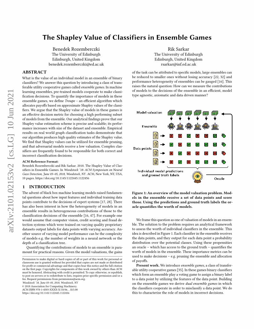
Figure 1: An overview of themodel valuation problem. Mod-els in the ensemble receive a set of data points and scorethose. Using the predictions and ground truth labels the or-acle quantifies the worth of models.

We frame this question as one of valuation of models in an ensem-

ble. The solution to the problem requires an analytical framework

to assess the worth of individual classifiers in the ensemble. This

idea is described in Figure 1. Each classifier in the ensemble receives

the data points, and they output for each data point a probability

distribution over the potential classes. Using these propensities

an oracle – which has access to the ground truth – quantifies the

worth of models in the ensemble. These importance metrics can be

used to make decisions – e.g. pruning the ensemble and allocation

of payoffs.

Present work.We introduce ensemble games, a class of transfer-able utility cooperative games [35]. In these games binary classifiers

which form an ensemble play a voting game to assign a binary label

to a data point by utilizing the features of the data point. Building

on the ensemble games we derive dual ensemble games in which

the classifiers cooperate in order to misclassify a data point. We do

this to characterize the role of models in incorrect decisions.

arX

iv:2

101.

0215

3v2

[cs

.LG

] 1

0 Ju

n 20

21

Woodstock ’18, June 03–05, 2018, Woodstock, NY Benedek Rozemberczki and Rik Sarkar

We argue that the Shapley value [41], a solution concept from

cooperative game theory, is a model importance metric. The Shap-

ley value of a classifier in the ensemble game defined for a data

point can be interpreted as the probability of the model becoming

the pivotal voter in a uniformly sampled random permutation of

classifiers. Computing the exact Shapley values in an ensemble

game would take factorial time in the number of classifiers. In order

to alleviate this we exploit an accurate approximation algorithm of

the individual Shapley values which was tailored to voting games

[12]. We propose Troupe, an algorithm which approximates the

average of Shapley values in ensemble games and dual games using

data. We utilize the average Shapley values as measures of model

importance in the ensemble and discuss that the Shapley values are

interpretable as an importance distribution over classifiers.

We evaluate Troupe by performing various classification tasks.

Using data from real world webgraphs (Reddit, GitHub, Twitch)

we demonstrate that Troupe outputs high quality estimates of the

Shapley value. We validate that the Shapley value estimates of

Troupe can be used as a decision metric to build space efficient and

accurate ensembles. Our results establish that more complex models

in an ensemble have a prime role in both correct and incorrect

decisions.

Main contributions. Specifically the contributions of our workcan be summarized as:

(1) We propose ensemble games and their dual games to model

the contribution of individual classifiers to the decisions of

voting based ensembles.

(2) We design Troupe an approximate Shapley value based algo-

rithm to quantify the role of classifiers in decisions.

(3) We provide a probabilistic bound for the approximation error

of average Shapley values estimated from labeled data.

(4) We empirically evaluate Troupe for model valuation and

forward ensemble building on graph classification tasks.

The rest of this work has the following structure. In Section 2 we

discuss related work on the Shapley value, its approximations and

applications in machine learning. We introduce the concept of en-

semble games in Section 3 and discuss Shapley value based model

valuation in Section 4 with theoretical results. We evaluate the

proposed algorithm experimentally in Section 5. We summarize our

findings in Section 6 and discuss future work. The reference imple-

mentation of Troupe is available at https://github.com/username/

repositoryname [Anonymized for double blind review].

2 RELATEDWORKOur model pruning framework intersects with research about the

Shapley value and existing approaches to ensemble pruning.

2.1 The Shapley valueThe Shapley value [41] is a solution to the problem of distributing

the gains among players in a transferable utility cooperative game

[35]. It is widely known for its desirable axiomatic properties [6]

such as efficiency and linearity. However, exact computation of

Shapley value takes factorial time, making it intractable in games

with a large number of players. General [29, 37] and game specific

[12] approximation techniques have been proposed. In Table 1, we

compare various approximation schemes with respect to certain

desired properties.

Shapley values can be approximated using a Monte Marlo MCsampling of the permutations of players and also with a truncated

Monte Carl sampling variant TMC [29, 30, 53]. A more tractable

approximation is proposed in [37], using a multilinear extension

(MLE) of the Shapley value. A variant of this technique [23, 24]

calculates the value of large players explicitly and applies the MLEtechnique to small ones. The only approximation technique tailored

to weighted voting games is the expected marginal contributions

method (EMC) which estimates the Shapley values based on contri-

butions to varying size coalitions. Our proposed algorithm Troupebuilds on EMC.

Table 1: Comparison of Shapley value computation and ap-proximation techniques in terms of having (✔) and missing(✘) desiderata; complexities with respect to the number ofplayers𝑚 and permutations 𝑝.

Method Voting Bound Non-Random Space TimeExplicit ✔ ✔ ✔ O(𝑚) O (𝑚!)MC [30] ✘ ✔ ✘ O(𝑚) O (𝑚𝑝)TMC [17] ✘ ✔ ✘ O(𝑚) O (𝑚𝑝)MLE [37] ✘ ✘ ✔ O(𝑚) O (𝑚)

MMLE [23, 24] ✘ ✘ ✔ O(𝑚) O (𝑚!)EMC [12] ✔ ✔ ✔ O(𝑚) O (𝑚2)

Shapley value has previously been used in machine learning for

measuring feature importance [8, 13, 21, 26, 27, 33, 38]. In the fea-

ture selection setting the features are seen as players that cooperate

to achieve high goodness of fit. Various discussed approximation

schemes [9, 29, 43] have been exploited to make feature importance

quantification in high dimensional spaces feasible [10, 28, 44, 45, 50]

when explicit computation is not tractable. Another machine learn-

ing domain for applying the Shapley value was the pruning of neu-

ral networks [1, 18, 42]. In this context approximate Shapley values

of hidden layer neurons are used to downsize overparametrized

classifiers. It is argued in [42] that pruning neurons is analogous to

feature selection on hidden layer features. Finally, there has been

increasing interest in the equitable valuation of data points with

game theoretic tools [17, 20]. In such settings the estimated Shap-

ley values are used to gauge the influence of individual points on

a supervised model. These approximate scores are obtained with

group testing of features [20] and permutation sampling [5, 17].

2.2 Ensemble pruning and buildingWe compare Troupe to existing ensemble pruning and bulding

approaches in terms of desired properties in Table 2. As one can see

our framework is the only one which has all of these characteristics.

Specifically, these properties are:

• Agnostic: The procedure can prune/build ensembles of het-

erogeneous model types, not just a specific type (e.g. trees).

• Set based: An algorithm is able to return a subset of models

with a high-performance, not just a single one.

• Diverse: The value of individual models is implicitly or ex-

plicitly affected by how diverse their predictions are.

The Shapley Value of Classifiers in Ensemble Games Woodstock ’18, June 03–05, 2018, Woodstock, NY

• Bidirectional: A bidirectional ensemble selection technique

can select a sub-ensemble in a forward or backward manner.

Table 2: Comparison of ensemble pruning and building tech-niques in terms of having (✔) and missing (✘) desiderata.

Method Agnostic Set based Diverse BidirectionalGreedy [4] ✔ ✔ ✘ ✔

WV-LP [51] ✔ ✔ ✘ ✘

RE [31] ✔ ✔ ✘ ✘

DREP [25] ✔ ✔ ✔ ✘

COMEP [2] ✘ ✔ ✔ ✘

EP-SDP [52] ✔ ✔ ✘ ✘

CART SySM [49] ✘ ✘ ✔ ✘

Troupe (ours) ✔ ✔ ✔ ✔

3 ENSEMBLES GAMESWe now introduce a novel class of co-operative games and examine

axiomatic properties of solution concepts which can be applied to

these games. We will discuss shapley value as an exact solution for

these games, [41], and discuss approximations of the Shapley value

based solution [12, 30, 37].

3.1 Ensemble gameWe define an ensemble game to be one where binary classifier mod-

els (players) co-operate to label a single data point. The aggregated

decision of the ensemble is assumed to be made by a vote of the

players. We assume that a set of labelled data points are known:

Definition 1. Labeled data point. Let (x, 𝑦) be a labeled datapoint where x ∈ R𝑑 is the feature vector and 𝑦 ∈ {0, 1} is the corre-sponding binary label.

Our work considers arbitrary binary classifier models (e.g. clas-

sification trees, support vector machines, neural networks) that

operate on the same input feature vector x. This approach is ag-

nostic of the exact type of the model, we only assume that𝑀 can

output a probability of the data point having a positive label. The

model owner does does not access the label, just a probability of

𝑦 = 1 is output by the model.

Definition 2. Positive classification probability for model𝑀 . Let (x, 𝑦) be a labeled data point and 𝑀 be a binary classifier,𝑃 (𝑦 = 1 | 𝑀, x) is the probability of the data point having a positivelabel output by classifier𝑀 .

We are now ready to define the operation of an ensemble classi-

fier consisting of multiple models.

Definition 3. Ensemble. An ensemble is a setM of size𝑚 thatconsists of binary classifier models 𝑀 ∈ M which can each outputa probability for a data point x ∈ R𝑑 having a positive label. Theensemble sets the probability of a label as:

𝑃 (𝑦 = 1 | M, x) =∑

𝑀 ∈M𝑃 (𝑦 = 1 | 𝑀, x)/𝑚.

And it makes decision about the label as:

𝑦 =

{1 if 𝑃 (𝑦 = 1 | M, x) ≥ 𝛾,0 otherwise.

where 0 ≤ 𝛾 ≤ 1 is the decision threshold and 𝑦 is the predicted labelof the data point.

Definition 4. Sub-ensemble. A sub-ensemble S is a subset S ⊆M of binary classifier models.

Definition 5. Individualmodel weight. The individual weightof the vote for 𝑀 , in sub-ensemble S ⊆ M for data point (𝑦, x) isdefined as:

𝑤𝑀 =

{𝑃 (𝑦 = 1 | 𝑀, x)/𝑚 if 𝑦 = 1,

𝑃 (𝑦 = 0 | 𝑀, x)/𝑚 otherwise.

Under this definition. the individual model weight of any binary

classifier𝑀 ∈ M is bounded: 0 ≤ 𝑤𝑀 ≤ 1/𝑚. Note that the weight

of𝑀 ∈ S depends on𝑚 – the size of the larger ensemble and not

on the size |S| of the sub-ensemble.

Definition 6. Ensemble game. LetM be a set of binary clas-sifiers. An ensemble game for a labeled data point (𝑦, x) is then aco-operative game 𝐺 = (M, 𝑣) in which:

𝑣 (S) ={1 if𝑤 (S) ≥ 𝛾,0 otherwise.

where𝑤 (S) = ∑𝑀 ∈S 𝑤𝑀 for any sub-ensemble S ⊆ M and thresh-

old 0 ≤ 𝛾 ≤ 1.

This definition is the central idea in our work. The models in the

ensemble play a cooperative voting game to classify the data point

correctly. When the data point is classified correctly the payoff is

1, an incorrect classification results in a payoff of 0. Each model

casts a weighted vote about the data point and our goal is going to

be to quantify the value of individual models in the final decision.

In other words, we would like to measure how individual binary

classifiers contribute on average to the correct classification of a

specific data point. This solution concept is described in the nextsection(3.2).

We can consider a misclassification as a dual ensemble game:

Definition 7. Dual ensemble game. LetM be a set of binaryclassifiers. A dual ensemble game for a labeled data point (𝑦, x) isthen a co-operative game 𝐺 = (M, ��) in which:

�� (S) ={1 if𝑤 (S) ≥ 𝛾,0 otherwise.

for a binary classifier ensemble vote score 0 ≤ 𝑤 (S) ≤ 1 where𝑤 (S) =

∑𝑀 ∈S (1/𝑚 − 𝑤𝑀 ) for any sub-ensemble S ⊆ M and

inverse cutoff value 0 ≤ 𝛾 ≤ 1 defined by 𝛾 = 1 − 𝛾 .

If the sum of classification weights for the binary classifiers

is below the cutoff value the models in the ensemble misclassify

the point, lose the ensemble game and as a consequence receive a

payoff that is zero. In such scenarios it is interesting to ask: how

can we describe the role of models in the misclassification? The

dual ensemble game is derived from the original ensemble game in

order to characterize this situation.

The classification game and its dual can be reframed simply as:

Definition 8. Simplified ensemble game. An ensemble gamein simplified form is described by the cutoff value – weight-vectortuple (𝛾, [𝑤1, . . . ,𝑤𝑚]).

Woodstock ’18, June 03–05, 2018, Woodstock, NY Benedek Rozemberczki and Rik Sarkar

Definition 9. Simplified dual ensemble game. Given a sim-plified form ensemble game (𝛾, [𝑤1, . . . ,𝑤𝑚]), the corresponding sim-plified dual ensemble game is defined by the cutoff value – weightvector tuple:

(𝛾, [𝑤1, . . . ,𝑤𝑚]) = (1 − 𝛾, [1/𝑚 −𝑤1, . . . , 1/𝑚 −𝑤𝑚])

The simplified forms of ensemble and dual ensemble games are

compact data structures which can describe the game without the

models themselves and the enumeration of every sub-ensemble.

3.2 Solution concepts for model valuationWe have defined the binary classification problemwith an ensemble

as a weighted voting game, which is a type of co-operative game.

Now we will argue that solution concepts of co-operative games

are suitable for the valuation of individual models which form the

binary classifier ensemble.

Definition 10. Solution concept. A solution concept defined forthe ensemble game 𝐺 = (M, 𝑣) is a function which assigns the realvalue Φ𝑀 (M, 𝑣) ∈ R to each binary classifier𝑀 ∈ M.

The scalar Φ𝑀 can be interpreted as the value of the individual

binary classifier𝑀 in the ensembleM. In the following we discuss

axiomatic properties of solution concepts which are the desiderata

for model valuation functions, and the implications of the axioms

in the context of model valuation in binary ensemble games.-edited

Axiom 1. Null classifier.A solution concept has the null classifierproperty if ∀ S ⊆ M : 𝑣 (S ∪ {𝑀}) = 𝑣 (S) then Φ𝑀 (M, 𝑣) = 0.

Having the null classifier property means that a binary classifier

which always has a zero marginal contribution in any sub-ensemble

will have a zero payoff on its own. This also implies that the classifier

never casts the deciding vote to correctly classify the data point

when it is added to a sub-ensemble. Conversely, in the dual ensemble

game the model never contributes to the misclassification of the

data point.

Axiom 2. Efficiency. A solution concept satisfies the efficiencyproperty if 𝑣 (M) = ∑

𝑀 ∈M Φ𝑀 (M, 𝑣).

That is, the value (loss or gain) of an ensemble can be split

precisely into the contributed value of the constituent models.

Axiom 3. Symmetry. A solution concept has the symmetry prop-erty if ∀S ⊆ M \ {𝑀 ′, 𝑀 ′′} : 𝑣 (S ∪ {𝑀 ′}) = 𝑣 (S ∪ {𝑀 ′′}) impliesthat Φ𝑀′ (M, 𝑣) = Φ𝑀′′ (M, 𝑣).

Two binary classifiers which make equal marginal contribution

to all sub-ensembles have the same value in the full ensemble.

Axiom 4. Linearity. A solution concept has the linearity propertyif given any two ensemble games 𝐺 = (M, 𝑣) and 𝐺 ′ = (M, 𝑣 ′) onthe same setM, the binary classifier 𝑀 satisfies Φ𝑀 (M, 𝑣 + 𝑣 ′) =Φ𝑀 (M, 𝑣) + Φ𝑀 (M, 𝑣 ′).

That is, the value in the combined game is the sum of the values

in individual games. This property will imply that valuations of a

model for different datapoints, when added, leads to its valuation

on the dataset.

3.3 The Shapley valueThe Shapley value [41] of a classifier is the average marginal con-

tribution of the model over the possible different permutations

in which the ensemble can be formed [6]. It is a solution concept

which satisfies Axioms 1-4 and the only solution concept which is

uniquely characterized by Axioms 3 and 4.

Definition 11. Shapley value. The Shapley value of binaryclassifier 𝑀 in the ensembleM, for the data point level ensemblegame 𝐺 = (M, 𝑣) is defined as

Φ𝑀 (𝑣) =∑

S⊆M\{𝑀}

|S |! ( |M | − |S | − 1)!|M |! (𝑣 (S ∪ {𝑀 }) − 𝑣 (S)) .

Calculating the exact Shapley value for every model in an ensem-

ble game would take O(𝑚!) time, or more, which is computationally

unfeasible in large ensembles. We discuss a range of approximation

approaches in detail which can give Shapley value estimates in

O(𝑚) and 𝑂 (𝑚2) time.

3.3.1 Multilinear extension (MLE) approximation of the Shapleyvalue. The MLE approximation of the Shapley value in a voting

game [12, 37] can be used to estimate the Shapley value in the

ensemble game and its dual game. Let us define the expectation

and the variation of the aggregated ensemble contributions for the

remaining models as: `𝑀 =∑𝑚𝑖=1𝑤 𝑗 − 𝑤𝑀 and a𝑀 =

∑𝑚𝑖=1𝑤

2

𝑗−

𝑤2

𝑀. For a classifier𝑀 ∈ M the multi-linear approximation of the

unnormalized Shapley value is computed by:

Φ𝑀 ∝𝛾∫

−∞

1

√2𝜋a𝑀

exp

(− (𝑥 − `𝑀 )

2

2a𝑀

)d𝑥 −

𝛾−𝑤𝑀∫−∞

1

√2𝜋a𝑀

exp

(− (𝑥 − `𝑀 )

2

2a𝑀

)d𝑥.

This approximation assumes that the size of the game is large

(many classifiers in the ensemble in our case) and also that ` has an

approximate normal distribution. Calculating all of the approximate

Shapley values by MLE takes O(𝑚) time.

3.3.2 Monte Carlo (MC) approximation of the Shapley value. TheMC approximation [29, 30] given the ensembleM estimates the

Shapley value of the model𝑀 ∈ M by the average marginal con-

tribution over uniformly sampled permutations.

Φ𝑀 = E\∼Θ [𝑣 (S𝑀\ ∪ {𝑀 }) − 𝑣 (S𝑀\) ] (1)

In Equation (1), Θ is a uniform distribution over the𝑚! permuta-

tions of the binary classifiers and S𝑀\

is the subset of models that

appear before the classifier 𝑀 in permutation \ . Approximating

the Shapley value requires the generation of 𝑝 classifier permuta-

tions (for a suitable 𝑝), and marginal contribution calculations with

respect to those contributions – this takes O(𝑚𝑝) time.

3.3.3 Voting game approximation of the Shapley value. The ensem-

ble games introduced above are a variant of voting games [36],

hence we can use the Expected Marginal Contributions (EMC) ap-proximation [12]. This procedure sums the expected marginal con-

tributions of a model to fixed size ensembles – it is described in the

pseudo-code Algorithm 1.

The algorithm iterates over the individual model weights and

initializes Shapley values as zeros (lines 1-2). For each ensemble size

it calculates the expected contribution of the model to the ensemble.

The Shapley Value of Classifiers in Ensemble Games Woodstock ’18, June 03–05, 2018, Woodstock, NY

(a) (b) (c) (d) (e)

Ensemble of binary classifiers

Data points

x1

x2

.

.

.

x𝑛

→→→→

Model owner 1

𝑃11= 𝑃 (𝑦1 = 1|x1, 𝑀1)

𝑃21= 𝑃 (𝑦2 = 1|x2, 𝑀1)

.

.

.

𝑃𝑛1= 𝑃 (𝑦𝑛 = 1|x𝑛, 𝑀1)

. . .

. . .

. . .

. . .;

Model ownerm

𝑃1𝑚 = 𝑃 (𝑦1 = 1|x1, 𝑀𝑚)

𝑃2𝑚 = 𝑃 (𝑦2 = 1|x2, 𝑀𝑚)

.

.

.

𝑃𝑛𝑚 = 𝑃 (𝑦𝑛 = 1|x𝑛, 𝑀𝑚);

→→→→

Label and scores

(𝑦1; [𝑃11, . . . , 𝑃1𝑚])

(𝑦2; [𝑃21, . . . , 𝑃2𝑚])

.

.

.

(𝑦𝑛 ; [𝑃𝑛1, . . . , 𝑃𝑛𝑚])

→→→→

Ensemble games

(𝛾 ; [w1

1, . . . ,w1

𝑚])

(𝛾 ; [w2

1, . . . ,w2

𝑚])

.

.

.

(𝛾 ; [w𝑛1, . . . ,w𝑛

𝑚])

→→→→

Shapley values

(Φ1,+1

, . . . , Φ1,+𝑚 )

(Φ2,+1

, . . . , Φ2,+𝑚 )

.

.

.

(Φ𝑛,+1

, . . . , Φ𝑛,+𝑚 )

(Φ1,−1

, . . . , Φ1,−𝑚 )

(Φ2,−1

, . . . , Φ2,−𝑚 )

.

.

.

(Φ𝑛,−1

, . . . , Φ𝑛,−𝑚 )

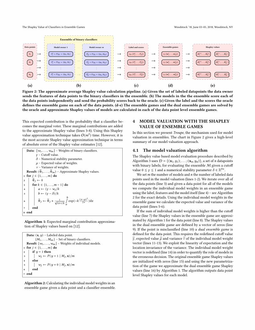
Figure 2: The approximate average Shapley value calculation pipeline. (a) Given the set of labeled datapoints the data ownersends the features of data points to the binary classifiers in the ensemble. (b) The models in the the ensemble score each ofthe data points independently and send the probability scores back to the oracle. (c) Given the label and the scores the oracledefines the ensemble game on each of the data points. (d-e) The ensemble games and the dual ensemble games are solved bythe oracle and approximate Shapley values of models are calculated in each of the data point level ensemble games.

This expected contribution is the probability that a classifier be-

comes the marginal voter. These marginal contributions are added

to the approximate Shapley value (lines 3-8). Using this Shapley

value approximation technique takes O(𝑚2) time. However, it is

the most accurate Shapley value approximation technique in terms

of absolute error of the Shapley value estimates [12].

Data: [𝑤1, . . . , 𝑤𝑚 ] – Weights of binary classifiers.

𝛾 – Cutoff value.

𝛿 – Numerical stability parameter.

` – Expected value of weights.

a – Variance of weights.

Result: (Φ1, . . . , Φ𝑚) – Approximate Shapley values.

1 for 𝑗 ∈ {1, . . . ,𝑚} do2 Φ𝑗 ← 0

3 for 𝑘 ∈ {1, . . . ,𝑚 − 1} do4 𝑎 ← (𝛾 − 𝑤𝑗 /𝑘5 𝑏 ← (𝛾 − 𝛿)/𝑘

6 Φ𝑗 ← Φ𝑗 + 1√2𝜋a/𝑘

𝑏∫𝑎

exp(−𝑘 (𝑥−`)2

2a)d𝑥

7 end8 end

Algorithm 1: Expected marginal contribution approxima-

tion of Shapley values based on [12].

Data: (x, 𝑦) – Labeled data point.

{𝑀1, . . . , 𝑀𝑚 } – Set of binary classifiers.

Result: [𝑤1, . . . , 𝑤𝑚 ] – Weights of individual models.

1 for 𝑗 ∈ {1, . . . ,𝑚} do2 if 𝑦 = 1 then3 𝑤𝑗 ← 𝑃 (𝑦 = 1 | 𝑀𝑗 , x)/𝑚4 else5 𝑤𝑗 ← 𝑃 (𝑦 = 0 | 𝑀𝑗 , x)/𝑚6 end7 end

Algorithm2:Calculating the individual model weights in an

ensemble game given a data point and a classifier ensemble.

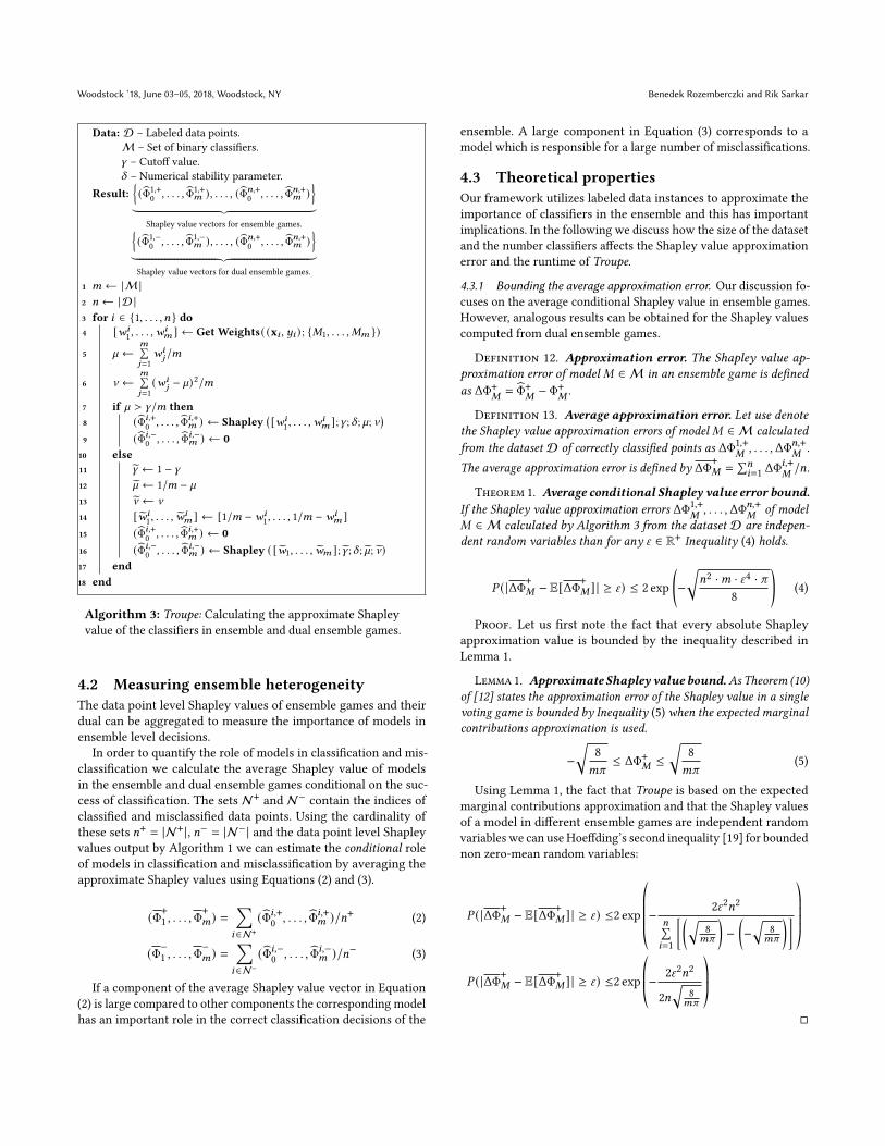
4 MODEL VALUATIONWITH THE SHAPLEYVALUE OF ENSEMBLE GAMES

In this section we present Troupe, the mechanism used for model

valuation in ensembles. The chart in Figure 2 gives a high-level

summary of our model valuation approach.

4.1 The model valuation algorithmThe Shapley value based model evaluation procedure described by

Algorithm 3 usesD = {(x1, 𝑦1); . . . ; (x𝑛, 𝑦𝑛)}, a set of 𝑛 datapoints

with binary labels, for evaluating the ensembleM given a cutoff

value 0 ≤ 𝛾 ≤ 1 and a numerical stability parameter 𝛿 ∈ R0+.We set𝑚 the number of models and 𝑛 the number of labeled data

points used in the model valuation (lines 1-2). We iterate over all of

the data points (line 3) and given a data point for all of the models

we compute the individual model weights in an ensemble game

using the label, features and the model itself (line 4) – see Algorithm

2 for the exact details. Using the individual model weights in the

ensemble game we calculate the expected value and variance of the

data point (lines 5-6).

If the sum of individual model weights is higher than the cutoff

value (line 7) the Shapley values in the ensemble game are approxi-

mated by Algorithm 1 for the data point (line 8). The Shapley values

in the dual ensemble game are defined by a vector of zeros (line

9). If the point is misclassified (line 10) a dual ensemble game isdefined for the data point. This requires the redefined cutoff value

𝛾 , expected value ˜and variance a of the individual model weight

vector (lines 11-13). We exploit the linearity of expectation and the

location invariance of the variance. The individual model weight

vector is redefined (line 14) in order to quantify the role of models in

the erroneous decision. The original ensemble game Shapley values

are initialized with zeros (line 15) and using the new parametriza-

tion of the game we approximate the dual ensemble game Shapley

values (line 16) by Algorithm 1. The algorithm outputs data point

level Shapley values for each model.

Woodstock ’18, June 03–05, 2018, Woodstock, NY Benedek Rozemberczki and Rik Sarkar

Data: D – Labeled data points.

M – Set of binary classifiers.

𝛾 – Cutoff value.

𝛿 – Numerical stability parameter.

Result:{(Φ1,+

0, . . . , Φ1,+

𝑚 ), . . . , (Φ𝑛,+0

, . . . , Φ𝑛,+𝑚 )

}︸ ︷︷ ︸

Shapley value vectors for ensemble games.{(Φ1,−

0, . . . , Φ1,−

𝑚 ), . . . , (Φ𝑛,+0

, . . . , Φ𝑛,+𝑚 )

}︸ ︷︷ ︸Shapley value vectors for dual ensemble games.

1 𝑚 ← |M |2 𝑛 ← |D |3 for 𝑖 ∈ {1, . . . , 𝑛} do4 [𝑤𝑖

1, . . . , 𝑤𝑖

𝑚 ] ← Get Weights( (x𝑖 , 𝑦𝑖 ) ; {𝑀1, . . . , 𝑀𝑚 })

5 ` ←𝑚∑𝑗=1

𝑤𝑖𝑗/𝑚

6 a ←𝑚∑𝑗=1(𝑤𝑖

𝑗− `)2/𝑚

7 if ` > 𝛾/𝑚 then8 (Φ𝑖,+

0, . . . , Φ𝑖,+

𝑚 ) ← Shapley([𝑤𝑖

1, . . . , 𝑤𝑖

𝑚 ];𝛾 ;𝛿 ; `; a)

9 (Φ𝑖,−0, . . . , Φ𝑖,−

𝑚 ) ← 010 else11 𝛾 ← 1 − 𝛾12 ˜← 1/𝑚 − `13 a ← a

14 [𝑤𝑖1, . . . , 𝑤𝑖

𝑚 ] ← [1/𝑚 − 𝑤𝑖1, . . . , 1/𝑚 − 𝑤𝑖

𝑚 ]15 (Φ𝑖,+

0, . . . , Φ𝑖,+

𝑚 ) ← 016 (Φ𝑖,−

0, . . . , Φ𝑖,−

𝑚 ) ← Shapley ( [𝑤1, . . . , 𝑤𝑚 ];𝛾 ;𝛿 ; ˜; a)17 end18 end

Algorithm 3: Troupe: Calculating the approximate Shapley

value of the classifiers in ensemble and dual ensemble games.

4.2 Measuring ensemble heterogeneityThe data point level Shapley values of ensemble games and their

dual can be aggregated to measure the importance of models in

ensemble level decisions.

In order to quantify the role of models in classification and mis-

classification we calculate the average Shapley value of models

in the ensemble and dual ensemble games conditional on the suc-

cess of classification. The sets N+ and N− contain the indices of

classified and misclassified data points. Using the cardinality of

these sets 𝑛+ = |N+ |, 𝑛− = |N− | and the data point level Shapley

values output by Algorithm 1 we can estimate the conditional roleof models in classification and misclassification by averaging the

approximate Shapley values using Equations (2) and (3).

(Φ+1, . . . ,Φ

+𝑚) =

∑𝑖∈N+(Φ𝑖,+

0, . . . , Φ𝑖,+𝑚 )/𝑛+ (2)

(Φ−1, . . . ,Φ

−𝑚) =

∑𝑖∈N−

(Φ𝑖,−0, . . . , Φ𝑖,−𝑚 )/𝑛− (3)

If a component of the average Shapley value vector in Equation

(2) is large compared to other components the corresponding model

has an important role in the correct classification decisions of the

ensemble. A large component in Equation (3) corresponds to a

model which is responsible for a large number of misclassifications.

4.3 Theoretical propertiesOur framework utilizes labeled data instances to approximate the

importance of classifiers in the ensemble and this has important

implications. In the following we discuss how the size of the dataset

and the number classifiers affects the Shapley value approximation

error and the runtime of Troupe.

4.3.1 Bounding the average approximation error. Our discussion fo-

cuses on the average conditional Shapley value in ensemble games.

However, analogous results can be obtained for the Shapley values

computed from dual ensemble games.

Definition 12. Approximation error. The Shapley value ap-proximation error of model𝑀 ∈ M in an ensemble game is definedas ΔΦ+

𝑀= Φ+

𝑀− Φ+

𝑀.

Definition 13. Average approximation error. Let use denotethe Shapley value approximation errors of model𝑀 ∈ M calculatedfrom the dataset D of correctly classified points as ΔΦ1,+

𝑀, . . . ,ΔΦ𝑛,+

𝑀.

The average approximation error is defined by ΔΦ+𝑀 =

∑𝑛𝑖=1 ΔΦ

𝑖,+𝑀/𝑛.

Theorem 1. Average conditional Shapley value error bound.If the Shapley value approximation errors ΔΦ1,+

𝑀, . . . ,ΔΦ𝑛,+

𝑀of model

𝑀 ∈ M calculated by Algorithm 3 from the dataset D are indepen-dent random variables than for any Y ∈ R+ Inequality (4) holds.

𝑃 ( |ΔΦ+𝑀 − E[ΔΦ+𝑀 ] | ≥ Y) ≤ 2 exp

(−√

𝑛2 ·𝑚 · Y4 · 𝜋8

)(4)

Proof. Let us first note the fact that every absolute Shapley

approximation value is bounded by the inequality described in

Lemma 1.

Lemma 1. Approximate Shapley value bound.As Theorem (10)of [12] states the approximation error of the Shapley value in a singlevoting game is bounded by Inequality (5) when the expected marginalcontributions approximation is used.

−√

8

𝑚𝜋≤ ΔΦ+𝑀 ≤

√8

𝑚𝜋(5)

Using Lemma 1, the fact that Troupe is based on the expected

marginal contributions approximation and that the Shapley values

of a model in different ensemble games are independent random

variables we can use Hoeffding’s second inequality [19] for bounded

non zero-mean random variables:

𝑃 ( |ΔΦ+𝑀 − E[ΔΦ+𝑀 ] | ≥ Y) ≤2 exp

©­­­­«− 2Y2𝑛2

𝑛∑𝑖=1

[(√8

𝑚𝜋

)−

(−√

8

𝑚𝜋

)] ª®®®®¬𝑃 ( |ΔΦ+𝑀 − E[ΔΦ

+𝑀 ] | ≥ Y) ≤2 exp

©­­«−2Y2𝑛2

2𝑛

√8

𝑚𝜋

ª®®¬□

The Shapley Value of Classifiers in Ensemble Games Woodstock ’18, June 03–05, 2018, Woodstock, NY

Theorem 2. Confidence interval of the expected average ap-proximation error. In order to acquire an (1−𝛼)-confidence intervalof E[ΔΦ+𝑀 ] ± Y one needs a labeled dataset D of correctly classifieddata points for which 𝑛 the cardinality of D, satisfies Inequality (6).

𝑛 ≥

√8 ln

2(𝛼2

)Y4𝑚𝜋

(6)

Proof. The probability 𝑃 ( |ΔΦ+𝑀 − E[ΔΦ+𝑀 ] | ≥ Y) in Theorem

1 equals to the level of significance for the confidence interval

E[ΔΦ𝑀+] ± Y. Which means that Inequality (7) holds for the signif-

icance level 𝛼 .

𝛼 ≤ 2 exp

(−√

𝑛2 ·𝑚 · Y4 · 𝜋8

). (7)

Solving inequality (7) for 𝑛 yields the cardinality of the dataset

(number of correctly classified data points) required for obtaining

the confidence interval described in Theorem 2. □

The inequality presented in Theorem 2 has two important con-

sequences regarding the bound:

(1) Larger ensembles require less data in order to give confident

estimates of the Shapley value for individual models.

(2) The dataset size requirement is sublinear in terms of con-

fidence level and quadratic in the precision of the Shapley

value approximation.

4.3.2 Runtime and memory complexity. The runtime and memory

complexity of the proposed model valuation framework depends

on the complexity of the main evaluation phases. We assume that

our framework operates in a single-core non distributed setting.

Scoring and game definition. Assuming that the scoring of a data

point takes O(1) time, scoring the data point with all models takes

O(𝑚). Scoring the whole dataset and defining games both takes

O(𝑛𝑚) time and O(𝑛𝑚) space respectively.Approximation and overall complexity. Calculating the expected

marginal contribution of a model to a fixed size ensemble takes

O(1) time. Doing this for all of the ensemble sizes takes𝑂 (𝑚) time.

Approximating the Shapley value for all models requires 𝑂 (𝑚2)time and𝑂 (𝑚) space. Given a dataset of 𝑛 points this implies a need

for𝑂 (𝑛𝑚2) time and𝑂 (𝑛𝑚) space. This is also the overall time and

space complexity of the proposed framework.

5 EXPERIMENTAL EVALUATIONIn this section, we show that Troupe approximates the average of

Shapley values precisely. We provide evidence that Shapley values

are a useful decision metric for ensemble creation. Our results

illustrate that model importance and complexity are correlated,

and that Shapley values are able to identify adversarial models

in the ensemble. Our evaluation is based on various real world

binary graph classification tasks [39]. Specifically, we use datasets

collected from Reddit, Twitch and GitHub – the descriptive statistics

of these datasets are in Table 3.

Table 3: Descriptive statistics of the graph classificationdatasets taken from [39] used for the evaluation of Troupe.

Classes Nodes Density DiameterDataset Positive Negative Min Max Min Max Min MaxReddit 521 479 11 93 0.023 0.027 2 18

Twitch 520 480 14 52 0.039 0.714 2 2

GitHub 552 448 10 942 0.004 0.509 2 15

5.1 The precision of approximationThe Shapley value approximation performance of Troupe is com-

pared to that of various other estimation schemes [29, 37] discussed

earlier. We use an ensemble of logistic regressions where each classi-

fier is trained on features extracted with a whole graph embedding

technique [40, 46, 48]. We utilize 50% of the graphs for training

and calculated the average conditional Shapley values of ensemble

games and dual ensemble games using the remaining 50% of the

data.

5.1.1 Experimental details. The features of the graphs are extractedwith whole graph embedding techniques implemented in the open

source Karate Club framework [39]. Given a set of graphs G =

(𝐺1, . . . ,𝐺𝑛) whole graph embedding algorithms [40, 46] learn a

mapping 𝑔 : G → R𝑑 which delineate the graphs 𝐺 ∈ G to a 𝑑

dimensional metric space. We utilize the following whole graph

embedding and statistical fingerprinting techniques:

(1) FEATHER [40] uses the characteristic function of topologi-

cal features as a graph level statistical descriptor.

(2) Graph2Vec [34] extracts tree features from the graph.

(3) GL2Vec [7] distills tree features from the dual graph.

(4) NetLSD [46] derives characteristics of graphs using the heat

trace of the graph spectra.

(5) SF [11] utilizes the largest eigenvalues of the graph Laplacianmatrix as an embedding.

(6) LDP [3] sketches the histogram of local degree distributions.

(7) GeoScattering [15] applies the scattering transform to var-

ious structural features (e.g. degree centrality).

(8) IGE [14] combines graph features from local degree distri-

butions and scattering transforms.

(9) FGSD [48] sketches the Moore-Penrose spectrum of the nor-

malized graph Laplacian with a histogram.

The embedding techniques use the default settings of the KarateClub library, each embedding dimension is column normalized and

the graph features are fed to the scikit-learn implementation of

logistic regression. This classifier is trained with ℓ2 penalty cost,

we choose an SGD optimizer and the regularization coefficient _

was set to be 10−2.

5.1.2 Experimental findings. In Table 4 we summarize the absolute

percentage error values (compared to exact Shapley values in en-

semble games) obtained with the various approximations schemes.

(i) Our empirical results support that Troupe consistently computes

accurate estimates of the ground truth model evaluations across

datasets and classifiers in the ensemble. (ii) The high quality of

estimates suggests that the approximate Shapley values of mod-

els extracted by Troupe can serve as a proxy decision metric for

ensemble building and model selection.

Woodstock ’18, June 03–05, 2018, Woodstock, NY Benedek Rozemberczki and Rik Sarkar

Table 4: Absolute percentage error of average conditional Shapley values obtained by approximation techniques (rows) for thegraph classifiers (columns) in the ensemble game. Bold numbers note the lowest error on each dataset – classifier pair.

Approximation FEATHER Graph2Vec GL2Vec NetLSD SF LDP GeoScatter IGE FGSD

Reddit

Troupe 1.23 2.35 8.18 0.99 2.64 2.31 1.64 4.85 1.49MLE 3.20 23.61 32.62 4.19 5.34 7.97 7.12 5.42 7.61

MC 𝑝 = 103

12.57 30.94 13.26 8.67 32.76 12.32 11.62 16.36 12.78

MC 𝑝 = 103

4.71 5.38 3.41 1.67 3.03 5.51 4.34 4.97 3.82

Twitch

Troupe 0.28 3.33 1.18 2.53 1.62 0.59 1.48 0.25 1.19

MLE 5.22 5.44 3.05 8.32 2.38 1.92 3.14 4.85 5.77

MC 𝑝 = 102

2.37 10.40 6.76 7.07 15.79 6.36 13.99 23.96 0.39MC 𝑝 = 10

32.32 4.60 2.96 2.67 2.53 2.73 6.31 0.27 3.89

GitHub

Troupe 2.68 0.18 2.61 1.41 1.49 1.23 1.88 2.36 1.04

MLE 9.22 5.12 3.76 3.27 9.71 7.46 5.08 4.04 0.73

MC 𝑝 = 102

5.91 9.37 4.67 9.82 8.78 8.34 13.66 28.95 0.76MC 𝑝 = 10

33.35 6.09 7.70 3.26 2.84 0.79 6.67 2.51 1.12

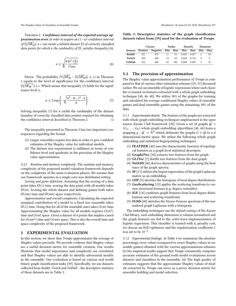
5.2 Ensemble buildingOur earlier results suggested that the approximate Shapley values

output by Troupe (and other estimation methods) can be used as

decision metrics for ensemble building.

0 10 20 30 40 50

0.50

0.60

0.70

0.80

Number of models

TestAUC

Reddit

Troupe MLE MC𝑝=102 MC𝑝=103

WV-LP RE DREP ED-SDP

0 10 20 30 40 50

0.50

0.54

0.58

0.62

Number of models

TestAUC

Twitch

Figure 3: The classification performance of ensembles as afunction of ensemble size selected by our forward modelbuilding procedure and baselines.

5.2.1 Experimental settings. We demonstrate this by selecting a

high performance subset of a random forest in a forward fashion

using the estimated model valuation scores. From each graph we

extract Weisfeiler-Lehman tree features [34] and keep those topo-

logical patterns which appeared in at least 5 graphs. Utilizing the

counts of these features in graphs we define statistical descriptors.

The selection procedure and evaluation steps are the following:

(1) Using 40% of the graphswe train a random forest with 50 clas-

sification trees, each tree is trained on 20 randomly sampled

Weisfeiler-Lehman features – we use the default settings of

scikit-learn.(2) We calculate the average conditional Shapley value of classi-

fiers in the games using 30% of the data.

(3) We order the classifiers by the approximate Shapley values in

decreasing order, create subensembles in a forward fashion

and calculate the predictive performance of the resulting

subensembles on the remaining 30% of the graphs.

The test performance (measured by AUC scores) of these classifiers

and baselines as a function of ensemble size is plotted on Figure 3.

5.2.2 Experimental findings. Our results suggest that Troupe has amaterial advantage over competing Shapley value approximation

schemes. Moreover, the proposed method outperforms the selection

of ensemble building baselines on the Twitch and Reddit datasets

[25, 31, 51, 52]. This implies that Troupe is a good alternative for

existing ensemble pruning techniques and our choice of the Shapley

value approximation scheme is justified in practical applications.

−4 −2 0 2 4

3

4

5

6

7

Normalized Shapley value

log2Hiddenlayerneurons

Ensemble gamesReddit

-4 -2 0 2 4

3

4

5

6

7

Normalized Shapley value

log2Hiddenlayerneurons

Dual ensemble gamesReddit

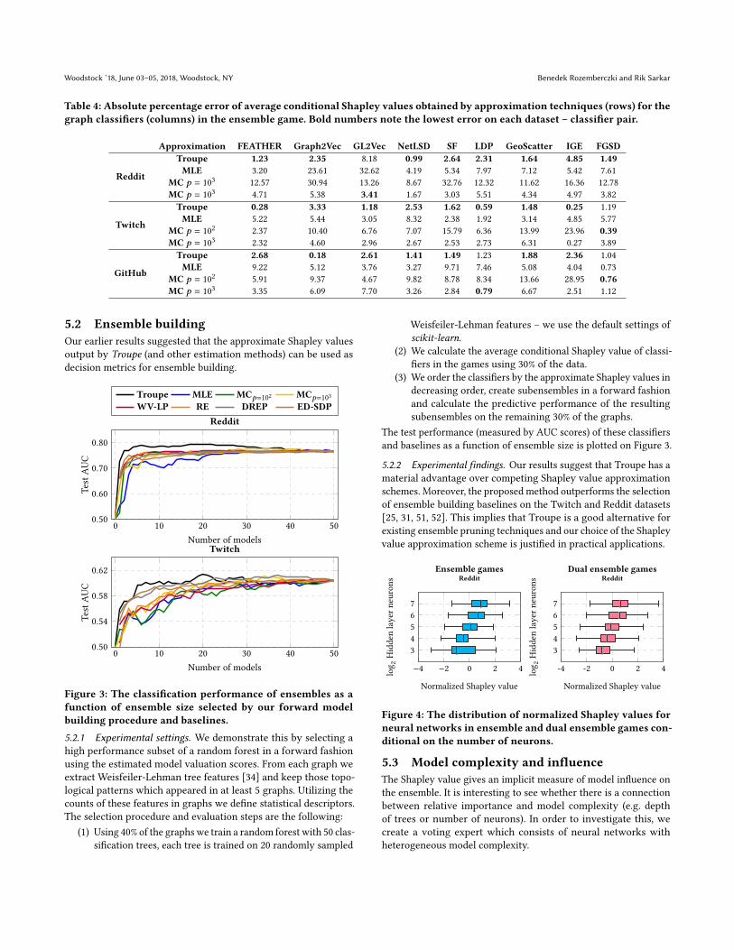
Figure 4: The distribution of normalized Shapley values forneural networks in ensemble and dual ensemble games con-ditional on the number of neurons.

5.3 Model complexity and influenceThe Shapley value gives an implicit measure of model influence on

the ensemble. It is interesting to see whether there is a connection

between relative importance and model complexity (e.g. depth

of trees or number of neurons). In order to investigate this, we

create a voting expert which consists of neural networks with

heterogeneous model complexity.

The Shapley Value of Classifiers in Ensemble Games Woodstock ’18, June 03–05, 2018, Woodstock, NY

5.3.1 Experimental settings. We create an ensemble of 𝑚 = 103

neural networks using scikit-learn – each of these has a single hid-

den layer. Each model receives 20 randomly selected frequency

features as input and has a randomly chosen number of hidden

layer neurons – we uniformly sample this hyperparameter from{23, 24, 25, 26, 27

}. Individual neural networks are trained by mini-

mizing the binary cross-entropy with SGD for 200 epochs with a

learning rate of 10−2.

5.3.2 Experimental findings. The distribution of normalized av-

erage Shapley values for the Reddit dataset are plotted on Figure

4 for the ensemble and dual ensemble games conditioned on the

number of hidden layer neurons. The results imply that more com-

plex models with a larger number of free parameters receive higher

Shapley values in both classes of games. In simple terms complex

models contribute to correct and incorrect classification decisions

at a disproportionate rate.

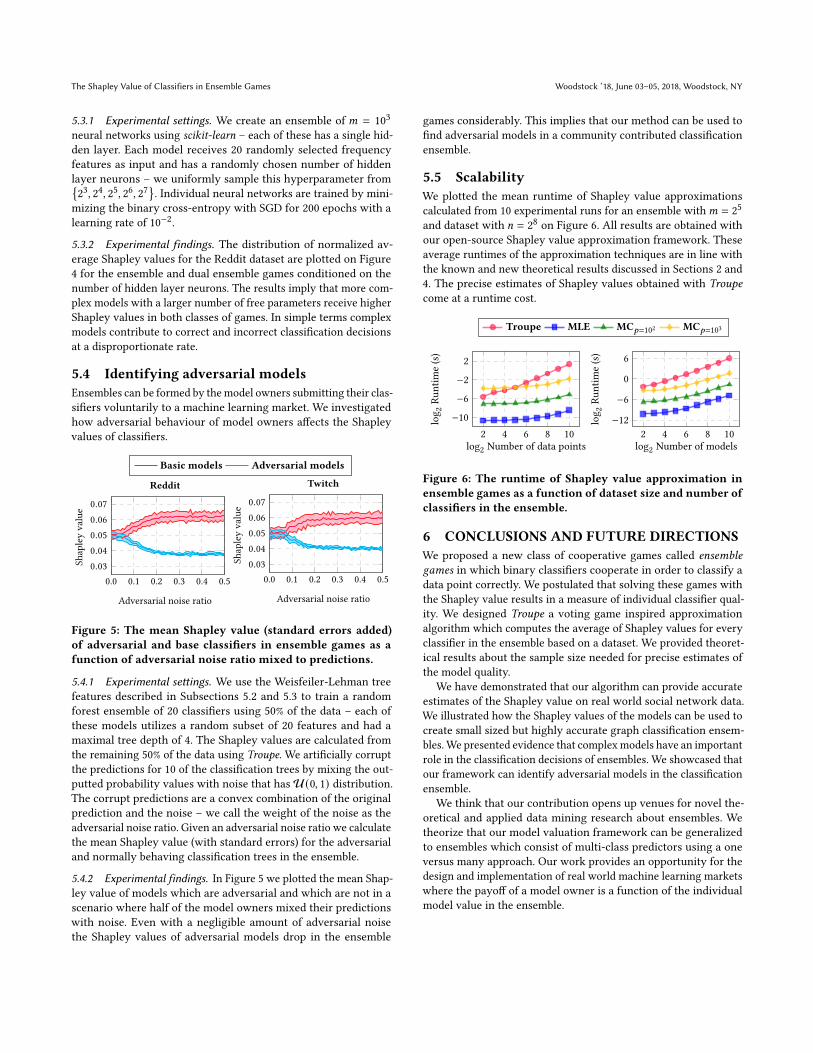
5.4 Identifying adversarial modelsEnsembles can be formed by themodel owners submitting their clas-

sifiers voluntarily to a machine learning market. We investigated

how adversarial behaviour of model owners affects the Shapley

values of classifiers.

0.0 0.1 0.2 0.3 0.4 0.5

0.03

0.04

0.05

0.06

0.07

Adversarial noise ratio

Shapleyvalue

Reddit

Basic models Adversarial models

0.0 0.1 0.2 0.3 0.4 0.5

0.03

0.04

0.05

0.06

0.07

Adversarial noise ratio

Shapleyvalue

Twitch

Figure 5: The mean Shapley value (standard errors added)of adversarial and base classifiers in ensemble games as afunction of adversarial noise ratio mixed to predictions.

5.4.1 Experimental settings. We use the Weisfeiler-Lehman tree

features described in Subsections 5.2 and 5.3 to train a random

forest ensemble of 20 classifiers using 50% of the data – each of

these models utilizes a random subset of 20 features and had a

maximal tree depth of 4. The Shapley values are calculated from

the remaining 50% of the data using Troupe. We artificially corrupt

the predictions for 10 of the classification trees by mixing the out-

putted probability values with noise that hasU(0, 1) distribution.The corrupt predictions are a convex combination of the original

prediction and the noise – we call the weight of the noise as the

adversarial noise ratio. Given an adversarial noise ratio we calculate

the mean Shapley value (with standard errors) for the adversarial

and normally behaving classification trees in the ensemble.

5.4.2 Experimental findings. In Figure 5 we plotted the mean Shap-

ley value of models which are adversarial and which are not in a

scenario where half of the model owners mixed their predictions

with noise. Even with a negligible amount of adversarial noise

the Shapley values of adversarial models drop in the ensemble

games considerably. This implies that our method can be used to

find adversarial models in a community contributed classification

ensemble.

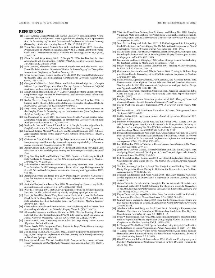
5.5 ScalabilityWe plotted the mean runtime of Shapley value approximations

calculated from 10 experimental runs for an ensemble with𝑚 = 25

and dataset with 𝑛 = 28on Figure 6. All results are obtained with

our open-source Shapley value approximation framework. These

average runtimes of the approximation techniques are in line with

the known and new theoretical results discussed in Sections 2 and

4. The precise estimates of Shapley values obtained with Troupecome at a runtime cost.

2 4 6 8 10

−10−6−22

log2Number of data points

log2Runtime(s)

Troupe MLE MC𝑝=102 MC𝑝=103

2 4 6 8 10

−12

−6

0

6

log2Number of models

log2Runtime(s)

Figure 6: The runtime of Shapley value approximation inensemble games as a function of dataset size and number ofclassifiers in the ensemble.

6 CONCLUSIONS AND FUTURE DIRECTIONSWe proposed a new class of cooperative games called ensemblegames in which binary classifiers cooperate in order to classify a

data point correctly. We postulated that solving these games with

the Shapley value results in a measure of individual classifier qual-

ity. We designed Troupe a voting game inspired approximation

algorithm which computes the average of Shapley values for every

classifier in the ensemble based on a dataset. We provided theoret-

ical results about the sample size needed for precise estimates of

the model quality.

We have demonstrated that our algorithm can provide accurate

estimates of the Shapley value on real world social network data.

We illustrated how the Shapley values of the models can be used to

create small sized but highly accurate graph classification ensem-

bles.We presented evidence that complexmodels have an important

role in the classification decisions of ensembles. We showcased that

our framework can identify adversarial models in the classification

ensemble.

We think that our contribution opens up venues for novel the-

oretical and applied data mining research about ensembles. We

theorize that our model valuation framework can be generalized

to ensembles which consist of multi-class predictors using a one

versus many approach. Our work provides an opportunity for the

design and implementation of real world machine learning markets

where the payoff of a model owner is a function of the individual

model value in the ensemble.

Woodstock ’18, June 03–05, 2018, Woodstock, NY Benedek Rozemberczki and Rik Sarkar

REFERENCES[1] Marco Ancona, Cengiz Oztireli, and Markus Gross. 2019. Explaining Deep Neural

Networks with a Polynomial Time Algorithm for Shapley Value Approxima-

tion. In Proceedings of the 36th International Conference on Machine Learning(Proceedings of Machine Learning Research), Vol. 97. PMLR, 272–281.

[2] Yijun Bian, Yijun Wang, Yaqiang Yao, and Huanhuan Chen. 2019. Ensemble

Pruning Based on Objection Maximization With a General Distributed Frame-

work. IEEE Transactions on Neural Networks and Learning Systems 31, 9 (2019),3766–3774.

[3] Chen Cai and Yusu Wang. 2018. A Simple Yet Effective Baseline for Non-

Attributed Graph Classification. ICLR 2019 Workshop on Representation Learningon Graphs and Manifolds (2018).

[4] Rich Caruana, Alexandru Niculescu-Mizil, Geoff Crew, and Alex Ksikes. 2004.

Ensemble Selection from Libraries of Models. In Proceedings of the Twenty-FirstInternational Conference on Machine Learning. 18.

[5] Javier Castro, Daniel Gómez, and Juan Tejada. 2009. Polynomial Calculation of

the Shapley Value Based on Sampling. Computers and Operations Research 36, 5

(2009), 1726 – 1730.

[6] Georgios Chalkiadakis, Edith Elkind, and Michael Wooldridge. 2011. Compu-

tational Aspects of Cooperative Game Theory. Synthesis Lectures on ArtificialIntelligence and Machine Learning 5, 6 (2011), 1–168.

[7] Hong Chen and Hisashi Koga. 2019. GL2Vec: Graph Embedding Enriched by Line

Graphs with Edge Features. In International Conference on Neural InformationProcessing. Springer, 3–14.

[8] Jianbo Chen, Le Song, Martin J Wainwright, and Michael I Jordan. 2018. L-

Shapley and C-Shapley: Efficient Model Interpretation for Structured Data. In

International Conference on Learning Representations.[9] Shay Cohen, Eytan Ruppin, and Gideon Dror. 2005. Feature Selection Based on

the Shapley Value. In Proceedings of the 19th International Joint Conference onArtificial Intelligence. 665–670.

[10] Ian Covert and Su-In Lee. 2021. Improving KernelSHAP: Practical Shapley Value

Estimation Using Linear Regression. In International Conference on ArtificialIntelligence and Statistics. PMLR, 3457–3465.

[11] Nathan de Lara and Pineau Edouard. 2018. A Simple Baseline Algorithm for

Graph Classification. In Advances in Neural Information Processing Systems.[12] Shaheen S Fatima, Michael Wooldridge, and Nicholas R Jennings. 2008. A Linear

Approximation Method for the Shapley Value. Artificial Intelligence 172, 14 (2008),1673–1699.

[13] Christopher Frye, Colin Rowat, and Ilya Feige. 2020. Asymmetric Shapley values:

incorporating causal knowledge into model-agnostic explainability. Advances inNeural Information Processing Systems 33 (2020).

[14] Alexis Galland and Marc Lelarge. 2019. Invariant Embedding for Graph Clas-

sification. In ICML Workshop on Learning and Reasoningwith Graph-StructuredData.

[15] Feng Gao, Guy Wolf, and Matthew Hirn. 2019. Geometric Scattering for Graph

Data Analysis. In Proceedings of the 36th International Conference on MachineLearning, Vol. 97. 2122–2131.

[16] Mike Gashler, Christophe Giraud-Carrier, and Tony Martinez. 2008. Decision

Tree Ensemble: Small Heterogeneous is Better than Large Homogeneous. In

Seventh International Conference on Machine Learning and Applications. IEEE,900–905.

[17] Amirata Ghorbani and James Zou. 2019. Data Shapley: Equitable Valuation of

Data for Machine Learning. In International Conference on Machine Learning.2242–2251.

[18] Amirata Ghorbani and James Zou. 2020. Neuron Shapley: Discovering the Re-

sponsible Neurons. arXiv preprint arXiv:2002.09815 (2020).[19] Wassily Hoeffding. 1994. Probability Inequalities for Sums of Bounded Random

Variables. In The Collected Works of Wassily Hoeffding. Springer, 409–426.[20] Ruoxi Jia, David Dao, BoxinWang, Frances AnnHubis, Nick Hynes, NeziheMerve

Gürel, Bo Li, Ce Zhang, Dawn Song, and Costas J. Spanos. [n.d.]. Towards Efficient

Data Valuation Based on the Shapley Value. In Proceedings of Machine LearningResearch. 1167–1176.

[21] Christophe Labreuche and Simon Fossier. 2018. Explaining Multi-Criteria Deci-

sion Aiding Models with an Extended Shapley Value. In IJCAI. 331–339.[22] Aleksandar Lazarevic and Zoran Obradovic. 2001. Effective Pruning of Neural

Network Classifier Ensembles. In IJCNN’01. International Joint Conference onNeural Networks. Proceedings (Cat. No. 01CH37222), Vol. 2. IEEE, 796–801.

[23] Dennis Leech. 1998. Computing Power Indices for Large Voting Games: A NewAlgorithm. Technical Report.

[24] Dennis Leech. 2003. Computing Power Indices for Large Voting Games. Manage-ment Science 49, 6 (2003), 831–837.

[25] Nan Li, Yang Yu, and Zhi-Hua Zhou. 2012. Diversity Regularized Ensemble Prun-

ing. In Joint European Conference on Machine Learning and Knowledge Discoveryin Databases. Springer, 330–345.

[26] Stan Lipovetsky and Michael Conklin. 2001. Analysis of Regression in Game

Theory Approach. Applied Stochastic Models in Business and Industry 17, 4 (2001),

319–330.

[27] Yifei Liu, Chao Chen, Yazheng Liu, Xi Zhang, and Sihong Xie. 2020. Shapley

Values and Meta-Explanations for Probabilistic Graphical Model Inference. In

Proceedings of the 29th ACM International Conference on Information & KnowledgeManagement. 945–954.

[28] Scott M. Lundberg and Su-In Lee. 2017. A Unified Approach to Interpreting

Model Predictions. In Proceedings of the 31st International Conference on NeuralInformation Processing Systems. Curran Associates Inc., 4768–4777.

[29] SasanMaleki, Long Tran-Thanh, GregHines, Talal Rahwan, andAlex Rogers. 2013.

Bounding the Estimation Error of Sampling-Based Shapley Value Approximation.

arXiv preprint arXiv:1306.4265 (2013).[30] Irwin Mann and Lloyd S Shapley. 1960. Values of Large Games, IV: Evaluating

the Electoral College by Monte Carlo Techniques. (1960).

[31] Dragos Margineantu and Thomas Dietterich. 1997. Pruning Adaptive Boosting.

In ICML, Vol. 97. Citeseer, 211–218.[32] Gonzalo Martínez-Muñoz and Alberto Suárez. 2006. Pruning in Ordered Bag-

ging Ensembles. In Proceedings of the 23rd International Conference on MachineLearning. 609–616.

[33] Fatiha Mokdad, Djamel Bouchaffra, Nabil Zerrouki, and Azzedine Touazi. 2015.

Determination of an Optimal Feature Selection Method Based on Maximum

Shapley Value. In 2015 15th International Conference on Intelligent Systems Designand Applications (ISDA). IEEE, 116–121.

[34] Annamalai Narayanan, Mahinthan Chandramohan, Rajasekar Venkatesan, Lihui

Chen, and Yang Liu. 2017. Graph2Vec: Learning Distributed Representations of

Graphs. (2017).

[35] Ludwig Johann Neumann, Oskar Morgenstern, et al. 1947. Theory of Games andEconomic Behavior. Vol. 60. Princeton University Press Princeton.

[36] Martin J Osborne and Ariel Rubinstein. 1994. A Course in Game Theory. MIT

press.

[37] Guillermo Owen. 1972. Multilinear Extensions of Games. Management Science18, 5-part-2 (1972), 64–79.

[38] Miklós Pintér. 2011. Regression Games. Annals of Operations Research 186, 1

(2011), 263–274.

[39] Benedek Rozemberczki, Oliver Kiss, and Rik Sarkar. 2020. Karate Club: An

API Oriented Open-source Python Framework for Unsupervised Learning on

Graphs. In Proceedings of the 29th ACM International Conference on Informationand Knowledge Management (CIKM ’20). ACM, 3125–3132.

[40] Benedek Rozemberczki and Rik Sarkar. 2020. Characteristic Functions on Graphs:

Birds of a Feather, from Statistical Descriptors to Parametric Models. In Proceed-ings of the 29th ACM International Conference on Information and KnowledgeManagement (CIKM ’20). ACM, 1325–1334.

[41] Lloyd S Shapley. 1953. A Value for n-Person Games. Contributions to the Theoryof Games 2, 28 (1953), 307–317.

[42] Julian Stier, Gabriele Gianini, Michael Granitzer, and Konstantin Ziegler. 2018.

Analysing Neural Network Topologies: A Game Theoretic Approach. ProcediaComputer Science 126 (2018), 234–243.

[43] Erik Strumbelj and Igor Kononenko. 2010. An Efficient Explanation of Individual

Classifications Using Game Theory. The Journal of Machine Learning Research11 (2010), 1–18.

[44] Xin Sun, Yanheng Liu, Jin Li, Jianqi Zhu, Xuejie Liu, and Huiling Chen. 2012.

Using Cooperative Game Theory to Optimize the Feature Selection Problem.

Neurocomputing 97 (2012), 86–93.

[45] Mukund Sundararajan and Amir Najmi. 2020. The Many Shapley Values for

Model Explanation. In International Conference on Machine Learning. PMLR,

9269–9278.

[46] Anton Tsitsulin, Davide Mottin, Panagiotis Karras, Alexander Bronstein, and

Emmanuel Müller. 2018. NetLSD: Hearing the Shape of a Graph. In Proceedingsof the 24th ACM SIGKDD International Conference on Knowledge Discovery andData Mining. ACM, 2347–2356.

[47] Kagan Tumer and Joydeep Ghosh. 1996. Error Correlation and Error Reduction

in Ensemble Classifiers. Connection Science 8, 3-4 (1996), 385–404.[48] Saurabh Verma and Zhi-Li Zhang. 2017. Hunt for the Unique, Stable, Sparse and

Fast Feature Learning on Graphs. In Advances in Neural Information ProcessingSystems. 88–98.

[49] Abraham Itzhak Weinberg and Mark Last. 2019. Selecting a Representative

Decision Tree from an Ensemble of Decision-Tree Models for Fast Big Data

Classification. Journal of Big Data 6, 1 (2019), 1–17.[50] Brian Williamson and Jean Feng. 2020. Efficient Nonparametric Statistical Infer-

ence on Population Feature Importance Using Shapley Values. In InternationalConference on Machine Learning. PMLR, 10282–10291.

[51] Li Zhang andWei-Da Zhou. 2011. Sparse Ensembles UsingWeighted Combination

Methods Based on Linear Programming. Pattern Recognition 44, 1 (2011), 97–106.[52] Yi Zhang, Samuel Burer, W Nick Street, Kristin P Bennett, and Emilio Parrado-

Hernández. 2006. Ensemble Pruning Via Semi-definite Programming. Journal ofMachine Learning Research 7, 7 (2006).

[53] Gilad Zlotkin and Jeffrey S. Rosenschein. 1994. Coalition, Cryptography, and

Stability: Mechanisms for Coalition Formation in Task Oriented Domains. In

AAAI. 432–437.