
On the Second Order Correction to the Ground State … · On the Second Order Correction to the...
104
B IRGER B RIETZKE On the Second Order Correction to the Ground State Energy of the Dilute Bose Gas X P HDTHESIS OCTOBER 2017 This thesis has been submitted to the PhD School of the Faculty of Science, University of Copenhagen.
Transcript of On the Second Order Correction to the Ground State … · On the Second Order Correction to the...

BIRGER BRIETZKE
On the Second Order Correction tothe Ground State Energy of the Dilute Bose Gas
X
PHD THESIS
OCTOBER 2017
This thesis has been submitted to the PhD School of the Faculty of Science,University of Copenhagen.

Birger BrietzkeDepartment of Mathematical SciencesUniversity of CopenhagenUniversitetsparken 5DK-2100 København ØDenmark
Advisor: Jan Philip SolovejUniversity of Copenhagen, Denmark
Assessment committee: Bergfinnur Duurhus (Chairman)University of Copenhagen, Denmark
Robert SeiringerIST Austria, Austria
Horia D. CorneanAalborg University, Denmark
This work is partially supported by the Villum Centre for the Mathematics of Quantum Theory (QMATH)
and the ERC Advanced grant 321029.
c© 2017 Birger Brietzke, except for the second part containing the manuscript:The Second Order Correction to the Ground State Energy of the Dilute Bose GasAuthors: Birger Brietzke and Jan Philip Solovejc© 2017 by the authors
ISBN Number: 978-87-7078-932-5

iii
Summary
In this thesis we consider a gas of interacting, identical, spin-less bosons in a thermodynamic box.
We are interested in the ground state energy, which for low densities (diluteness) is described by
the Lee–Huang–Yang (LHY) formula – a series expansion in the density that has been derived
from Bogolubov’s work in the late 1950’s.
In the introduction we discuss how to derive the LHY formula using Bogolubov’s approximation
step, which presupposes Bose-Einstein condensation. The second part contains a detailed proof,
which establishes the LHY formula as a lower bound in a weak coupling and low density regime.
While our proof is guided by Bogolubov’s predictions, it is based on a two-step localization
procedure, which allows us to prove adequate ’local condensation’.
Resume
I denne afhandling betragtes en gas af vekselvirkende, identiske bosoner uden spin i en termody-
namisk boks. Vi er interesseret i grundtilstandsenergien, som for lave densiteter beskrives ved
hjælp af Lee–Huang–Yang (LHY) formlen – en rækkeudvikling i densiteten, som blev udledt fra
Bogolubovs arbejde i slutningen af 1950’erne.
I introduktionen diskuteres en udledning af LHY-formlen baseret pa Bogolubovs approksima-
tion, som forudsætter Bose-Einstein-kondensation. I anden del af afhandlingen præsenteres et
detaljeret bevis, som etablerer LHY-formlen som nedre grænse i et regime med svag kopling og
lav densitet. Vores bevis tager afsæt i Bogolubovs forudsigelser, men er baseret pa en to-trins
lokaliseringsprocedure, som tillader os at vise en passende form for ’lokal kondensation’.

iv
Acknowledgements
First and foremost I would like to thank my advisor Jan Philip Solovej for suggestingthe topic for this thesis and the scientific guidance he has provided throughout my timeas his student. Next, I would like to thank Robert Seiringer for hosting me in his groupduring my stay abroad at the IST Austria near Vienna. In particular I would like tothank Simon and Thomas, who I shared an office with, for discussions on our projects,Robert’s course, life in Vienna and climbing.Back in Copenhagen, my group had transformed into being part of the new QMATH-center, which had the effect that there was a steady flow of incoming new colleagues.While I enjoyed interacting with all of QMATH, I am only going to mention my groupmembers: Niels Benedikter, Jeremy Sok, Fabian Portman, Angelo Lucia, Albert Werner,Giacomo De Palma, Robin Reuvers, Anton Samojlow, Sabiha Tokus, Lukas Schimmerand Laurent Betermin for the numerous activities (seminars, group meetings, lectures,conferences, the running group and more) over the years. Special thanks go to LukasSchimmer for remarks and advice on the draft for this thesis.
Further I would like to extend my thanks to Christian Majenz, Giacomo Cherubini,Nicholas Gauguin Houghton-Larsen, Mathias Makedonski and Asger Kjærulff Jensen,who I shared my office with. Last but not least, I want to thank my family for the loveand support I have received over the years.

Contents
PrefaceSummary iiiResume iiiAcknowledgements iv
Part I. Introduction 71. Introduction 82. Background 103. Aspects of Bogolubov Theory 154. Upper and Lower Bounds 205. A New Lower Bound 21
References 35
Part II. Manuscript 39
The Second Order Correction to the Ground State Energy of the Dilute Bose Gas 41
5


Part I
Introduction

1. INTRODUCTION 8
At the bottom of the spectrum lives a ground state energythe one for interacting bosons without entropyin the density limit – the dilutewe calculate a constanthopefully importantusing operators – which do not commute
– B. Brietzke
1. Introduction
The introduction of Bose gases and the prediction of Bose-Einstein condensates goesback to S. N. Bose [6] and A. Einstein [11] almost one century ago. By condensationwe mean macroscopic occupation of a single particle state. In sharp contrast to bosons,this is not possible for identical fermions; a fact known as the Pauli exclusion principle.One of the reasons why Bose-Einstein condensation is interesting, lies in its connectionto liquid Helium and its superfluidity. N. N. Bogolubov1 attempted to explain thisconnection in his seminal paper from 1947 [5]. Since Bose-Einstein condensation onlyoccurs in gases at very low temperatures and low density, several cooling methods had tobe developed and then combined to create Bose-Einstein condensates in the laboratory.This experimental breakthrough happened in 1995, more than 70 years after Einstein’sprediction. Experiments by the groups of E. A. Cornell and C. E. Wiemann confirmedthe existence of Bose-Einstein condensates. Independently W. Ketterle produced a Bose-Einstein condensate in a slightly different set-up. The experiments, performed at around20 nK were honoured with the Nobel Prize in 2001 [36]. Already at that time more than20 groups had managed to produce Bose-Einstein condensates and the experimentalinterest intensified. At the time of writing this thesis, a search for “Bose-Einstein” hasyielded more than 20.000 publications2.
As one can read in [2], condensates have been created for a wide range of vapors withtypical sizes between 1.5 × 10³ and 106 atoms. Possibly inspired by the experimentalsuccess, there has also been an increase in theoretical work on Bose gases in the lastdecades. We refer to [25] for an overview of the mathematical work on the Bose gas andto [38, 39] for a physics point of view.
In this thesis we will restrict our interest to only one of the most fundamentalquantities of a Bose gas – the ground state energy. More specifically:
How does the ground state energy of a dilute Bose gas at zero temperaturedepend on the density?
An answer to this question is essentially contained in Bogolubov’s approximationand known as the Lee–Huang–Yang formula [21, 22], which describes the low densityasymptotics of the ground state energy per volume in the thermodynamic limit, e0(ρ).The core of Bogolubov’s theory is a very fruitful but non-rigorous diagonalization of theHamiltonian. We will discuss Bogolubov’s approximation step, which is well-motivatedby the physics involved. One of the insights of Bogolubov is that the ground state energy
1Note that “Bogolubov” is not the only transliteration, which is used in the literature.2The publication database webofknowledge.com was used with the search term “Bose-Einstein” on the27.10.2017.

1. INTRODUCTION 9
only depends on the potential via the scattering length, a. Our aim is to show that theLee–Huang–Yang formula, which reads
e0(ρ) = 4πνρ2a
(1 +
128
15√π
(ρa3)12 + o(
√ρa3)
)as ρa3 → 0, (1.1)
with ν = ~2
2m , is correct as a lower bound. To succeed, we will of course have to posesome restrictions on the class of potentials. Also we have to introduce an additionalscaling to obtain our result. Concerning the rigorous proof of the lower bound, this isthe second step forward towards establishing (1.1).
This is not merely a theoretical result, however. In experiments by Navon et al.[34, 35] the LHY-constant has been measured by changing the scattering length usingFeshbach resonances. The measurements, 4.4(5), respectively 4.5(7), were in agreementwith the predicted value 128
15√π≈ 4.81. Also the Monte Carlo computations in [15] match
the theoretical prediction well, if the LHY-correction term is included.
We end this introduction with an overview of the further sections in the present thesis:In Section 2, the background chapter, we fix notation and present mathematical back-ground needed to formalize the description of the dilute Bose gas. The Hamiltonian forthe system is introduced in position space and rewritten in second quantized form. Thisexpression gives a heuristic argument for the leading order term of the ground stateenergy.In Section 3 we present a calculation for the second order correction term (LHY-term)using the concept of c-number substitution, which is based on a condensation hypothesis,is used. This calculation invokes an approximation of the scattering length of the po-tential and can therefore only be correct in a certain scaling limit.In Section 4 related mathematical literature on ground state energies for dilute Bosegases is reviewed.In Section 5 we state the main result of this thesis:
For a broad range of potentials the LHY formula is correct as a lower bound for theground state energy of a dilute Bose gas in a scaling regime, which goes beyond the
mean inter-particle distance.
We present key ingredients leading to the proof of this statement. Furthermore, wepoint out some technical difficulties, which are responsible for the assumptions in ourmain theorem and conclude with remarks on possible improvements in future work.Part II consists of the manuscript containing the mathematical proof for the mentionedresult. This is an improvement compared to the work by Giuliani and Seiringer [17],who gave the until now only available proof for a lower bound capturing the secondorder correction.

2. BACKGROUND 10
2. Background
This section provides some background for the mathematical treatment of the Bosegas. Relevant length scales associated to gas are discussed and the corresponding manybody Hamiltonian is rewritten in second quantized form using creation and annihilationoperators. This standard bookkeeping method is then used to describe Bogolubov’sc-number substitution and how it leads to the prediction that the ground state energyin the dilute limit is given by (1.1). This section is based on [25] and [44]. For additionalbackground material the reader is referred to [12, 26, 42] and [43].
We consider a gas of N interacting particles. Particles in a interacting gas may besubject to both an external potential, e.g. some trap, which confines the gas to a regionin space and an interaction-potential. Such a gas can be modelled by the Hamiltonian
HN =N∑
i=1
(−∆i + Vext,i) + Vint, (2.1)
which acts on the space L2(R3N ), i.e., the Hilbert space of square-integrable functions onR3N . We use the convention 〈f, g〉 :=
∫f(x)g(x) dx for the inner product of the functions
f, g ∈ L2(R3N ). Here ∆if =3∑j=1
∂2f∂x2j, with xi = (x1, x2, x3) ∈ R3, is the Laplacian acting
on the ith particle. All Hilbert spaces that we will encounter in this thesis are goingto be separable and infinite dimensional. Vectors of length unity play a special role. If||ψ||2 = 1, we call ψ a wave function and interpret the quantity
|ψ(x1, x2, . . . , xN )|2 (2.2)
as the probability density for finding particle 1 at x1, particle 2 at x2 etc. Measurementscorrespond to self-adjoint operators. If the measurement corresponds to the (possiblyunbounded) self-adjoint operator A and is performed on the state ψ, then
〈A〉ψ := 〈ψ,Aψ〉 (2.3)
is the expectation value for the measurement. The possible outcomes for a measurementare the elements in the spectrum of A
spec (A) := λ ∈ C : (A− λ1) has no bounded inverse , (2.4)
which is contained in R if the operator is self-adjoint. Note that we in (2.3) do not haveto require ψ ∈ D (A), but only that ψ is contained in the domain of the quadratic formcorresponding to A. We only consider gases of identical bosons and these satisfy, bydefinition, the symmetry condition
ψ(x1, x2, . . . , xN ) = ψ(xσ1 , xσ2 , . . . , xσN ) (2.5)
for any permutation σ = (σ1, σ2, . . . , σN ) in the permutation group SN of N elements3.Henceforth we will only consider Bose gases constrained to some box, say Λ = [−L
2 ,L2 ]3,
3For systems in two spacial dimensions interchanging two identical particles can give a phase other than±1, which shows that particle species other than fermions and bosons exist. Such particles are calledanyons – a term coined by Frank Wilczek [46] – reflecting that indeed the ”interchange of two of theseparticles can give any phase.”

2. BACKGROUND 11
with side length L > 0. Instead of setting
Vext(x) =
0 if x ∈ Λ
∞ if x /∈ Λ,(2.6)
we simply drop the external potential and restrict our interest to the Hilbert space ofpermutation symmetric functions in L2(Λ) with Dirichlet boundary conditions. We thenhave
HN = −νN∑
i=1
∆i +∑
1≤i<j≤NV (|xi − xj |), (2.7)
with ν = ~2
2m , where m is the mass of a particle and ~ denotes the reduced Planck’sconstant. The density of a gas is defined by the number of particles per volume
ρ =N
|Λ| . (2.8)
For notational convenience, we henceforth choose units such that ν = ~2/(2m) = 1.
2.1. Ground States and Grounds State Energies
The ground state energy of N interacting particles in the box Λ = [−L2 ,
L2 ]3 is
E0(N,L) := infΨ∈Q(HN )||Ψ||=1
〈Ψ, HNΨ〉 = inf spec (HN ) , (2.9)
where Q (HN ) is the domain of the quadratic form corresponding to HN . Note that theinfimum in (2.9) not necessarily has to be attained or to be finite. In case E0(N,L) isfinite, then the N -body system is called stable. We call ψ a ground state if it satisfies〈ψ,HNψ〉 = E0(N,L) and it can be shown that ψ is a ground state if and only if ψ is asolution to the Schrodinger equation HNψ = E0(N,L)ψ. Our primary interest is to finda new second order lower bound for the energy per unit volume in the thermodynamiclimit,4
e0(ρ) := limN,L→∞N/L3=ρ
E0(N,L)L−3. (2.10)
To obtain a heuristic understanding of the problem at hand, it is useful to considerwhich length scales are relevant. These are:
a: the scattering length,
(ρa)−12 : the correlation length5,
ρ−13 : the mean inter-particle distance.
While the mean inter-particle distance simply is the order of the average distance to thenext particle, the other two length scales require some explanation.
The correlation length can be understood in the following way. If the particles arelocalized to boxes of side length λc, then the uncertainty principle gives an energy of
4In Part II we use the less restrictive requirement N,L→∞ with limN,L→∞
NL−3 = ρ.
5This length scale is also known as the uncertainty principle length, healing length, de Broglie wavelengthor the Bogolubov length.

2. BACKGROUND 12
order λ−2c . The energy per volume is then at least Nλ−2
c L−3 = ρλ−2c , which is compa-
rable to the leading order term 4πaρ2 in (1.1) if λc = 1√ρa .
We will see below that the scattering length a is a constant depending on the poten-tial at hand. Since we are interested in the dilute limit, we have ρa3 1. In particular,
we have ρ−13 1√
ρa . Hence, for states close to the ground state, we can only localize
particles to boxes which are much larger than the mean inter-particle distance, showingthat the wave functions overlap considerably for low densities.
2.2. The Scattering Length
We follow [25] and define the scattering length, which is a measure for the effectiveinteraction strength of a potential. For simplicity we assume that W ≥ 0, that W isspherically symmetric and that W (x) = 0 if |x| > R0 for some R0. These assumptionsare less restrictive than those we have in Part II. In fact, the first and the third assump-tion can be relaxed [25].
The boundary of the ball BR is denoted SR and has surface area 4πR2. Todiscuss the two-body problem, we define on
φ ∈ H1 (BR) : φ(x) = 1 for x ∈ SR
, where
R > R0, the map ER by
ER[φ] =
∫
BR
|∇φ(x)|2 +1
2W (x)|φ(x)|2 dx. (2.11)
One can show that ER has a unique minimizer, 0 ≤ φ0 ≤ 1, which is spherically sym-metric and radially increasing. Equation (2.11) is related to the zero-energy scatteringequation
−∆φ0(x) +1
2W (x)φ0(x) = 0. (2.12)
That this equation holds in the sense of distributions on BR follows from the followingstandard computation [25]. Let ψ ∈ C∞0 (BR) and note that
ER [φ0 + δψ] = ER [φ0] + δ2ER [ψ] + 2δRe
∫
BR
∇φ0 · ∇ψ +1
2Wφ0ψ dx. (2.13)
Because φ0 is a minimizer for ER, integration by parts yields
0 =d
dδER [φ0 + δψ]|δ=0 = 2Re
∫
BR
∇φ0 · ∇ψ +1
2Wφ0ψ dx
= 2Re
∫
BR
ψ
[−∆φ0 +
1
2Wφ0
]dx+
∫
SR
ψ∇φ0 · dS. (2.14)
The last term in (2.14) vanishes because ψ ∈ C∞0 (BR) and the claim follows by repeatingthe argument with ψ replaced by iψ. An other way to state the above is that we employthe the Euler-Lagrange equation.
On the annulus AR0,R :=x ∈ R3 : R0 < |x| < R
the scattering equation reduces
to the requirement that φ0 is harmonic. Combining this with the boundary conditionφ(x) = 1 for x ∈ SR, we obtain on AR0,R that
φ0(x) =1− a
|x|1− a
R
, a ∈ [0, R0]. (2.15)
The constant a is called the scattering length and is determined by the value of φ0 onSR0 , i.e., the inner boundary of the above annulus, and depends on the potential through

2. BACKGROUND 13
the scattering equation (2.12). The two examples below show that the scattering lengthindeed is a reasonable measure for the interaction range of the potential.
The minimum energy for ER is found using the scattering equation (2.12) and inte-gration by parts
ER[φ0] =
∫
BR
|∇φ0|2 +1
2W |φ0|2 dx
=
∫
SR
φ0∇φ0 · dS +
∫
BR
φ0
[−∆φ0 +
1
2W (x)φ0
]dx
= 4πa(1− a
R)−1. (2.16)
The leading order term 4πρ2a in the LHY formula can, at least heuristically, be un-derstood in the following way. The minimization problem (2.11) originates from thetwo-body problem via a center of mass integration such that φ0 describes the relativeposition of the two particles. See [42] for an exposition. Because 〈φ0, φ0〉 is of order R3
we make the ansatz
limR→∞
R3E0(2, R) = 8πa. (2.17)
We now obtain
e0(ρ) = limN,R→∞N/R3=ρ
E0(N,R)R−3 ≈ limN,R→∞N/R3=ρ
8πaN(N − 1)
2R−6 = 4πρ2a, (2.18)
if we assume that energy is approximately linear in the number of pairs. This assumptionneglects the interaction between the pairs. It is therefore reasonable, form the viewpointof this heuristic description, that the second order correction term in the LHY formulais positive.
Example 1: For the hard-core potential with radius R0, i.e.,
WR0(x) =
∞ if |x| < R0
0 if |x| ≥ R0,(2.19)
we have φ0(x) = 0 for x ∈ BR0 such that the scattering length agrees with the range ofthe potential; a = R0.
Example 2: In the non-interacting case the scattering length vanishes. This is be-cause φ0 = 1BR if W = 0 and it then follows from (2.15) that a = 0.
The converse is also true. If a = 0, we have by (2.15) that φ0 = 1 on AR0,R. Thefunction φ0 is subharmonic on BR since W is positive. Because φ0 attains its maximumon the interior of BR, it follows from the maximum principle that φ0 is constant. Thusφ0 = 1BR , and consequently 0 = ER (1BR) =
∫W = 0. From the positivity of W we
obtain W = 0.
For these two extreme examples we easily found values for the scattering lengthwhich make sense from a physics point of view. A natural question is:
Does the scattering length increase as the potential increases?
The answer is yes. Here we give a modified version of the proof of Lemma C.3 in[25], where it is proven using contradiction.

2. BACKGROUND 14
Let (V, φ0, a) and (V , φ0, a) be triples consisting of potential, scattering solution and
scattering length satisfying V ≥ V ≥ 0. Then we have a ≥ a.It follows from the scattering equation (2.12) that the difference of the scattering
solutions, g := φ0 − φ0, is subharmonic. Hence g attains its maximum on SR. Since
φ0(x) = φ0(x) = 1 for x ∈ SR, we have φ0 ≥ φ0 and therefore a ≥ a.
2.3. Fock Space
We now introduce Fock space [14], which is a standard technical tool and allowsone to deal with variable particle numbers. Given a Hilbert space H, we define H0 = C,H1 = H and HN = HN−1 ⊗H for N > 1. On HN we define the orthogonal projections
P+N (ψ1 ⊗ ψ2 ⊗ · · · ⊗ ψN ) =
∑
σ∈SN
1
N !ψσ1 ⊗ ψσ2 ⊗ · · · ⊗ ψσN , (2.20)
P−N (ψ1 ⊗ ψ2 ⊗ · · · ⊗ ψN ) =∑
σ∈SN
(−1)|σ|
N !ψσ1 ⊗ ψσ2 ⊗ · · · ⊗ ψσN , (2.21)
where |σ| is the order of the permutation σ ∈ SN . The Fock space is the Hilbert space
F =∞⊕
N=0
HN . (2.22)
Using the projections in (2.20), respectively (2.21), we define the bosonic, respectivelyfermionic, Fock spaces
F+ =
∞⊕
N=0
N⊗
i=1sym
H :=
∞⊕
N=0
N⊗P+N (HN ) , (2.23)
F− =∞⊕
N=0
N∧
i=1
H :=∞⊕
N=0
N⊗P−N (HN ) . (2.24)
The vector |Ω〉 = 1 ∈ C plays a special role and is often called the vacuum. Sometimesit is convenient to specify a state, i.e., a normalized vector in F by letting creation andannihilation operators act on the vacuum state. By linearity it suffices to define how theannihilation operator, a(f), maps pure tensors in the N -particle sector HN into HN−1
and the creation operator, a∗(f) := (a(f))∗, maps pure tensors in HN into HN+1
a(f)(f1 ⊗ f2 ⊗ · · · ⊗ fN ) = N12 〈f |f1〉f2 ⊗ f3 ⊗ · · · ⊗ fN , (2.25)
a∗(f)(f1 ⊗ f2 ⊗ · · · ⊗ fN ) = (N + 1)12 f ⊗ f1 ⊗ · · · ⊗ fN . (2.26)
We then have that H 3 f 7→ a∗(f) is linear and that f 7→ a(f) is anti-linear. Note thatthe restriction of a(f), respectively a∗(f), to any N -particle sector defines a boundedoperator, while a(f) is an unbounded operator defined on the domain
ψ =
∞⊕
N=0
ψN
∣∣∣∞∑
N=0
N ||ψN ||2 <∞. (2.27)

3. ASPECTS OF BOGOLUBOV THEORY 15
We also note that the operators a(f) preserve symmetry, respectively anti-symmetry;but that the operators a(f)∗ do not. That is
ψ ∈ F± ; a(f)∗ψ ∈ F±. (2.28)
When working on the bosonic/fermionic Fock space, F±, this problem is circumventedby projecting down onto F± after applying a(f)∗.
2.1. DEFINITION (Bosonic and fermionic creation operator).For f ∈ H, we define the bosonic and fermionic creation operator by
a±(f)∗ = P± (a(f)∗) . (2.29)
Given an operator h on H, we will let hi denote the operator acting on the ith copy
of H in the N -particle sector HN =N⊗i=1H, i.e.,
hi = 1H ⊗ · · · ⊗ 1H ⊗ hith factor
⊗ 1H ⊗ · · · ⊗ 1H (2.30)
and define on F the second quantization of the one-particle operator h by
Γ (h) :=
∞⊕
N=1
N∑
i=1
hi. (2.31)
If the Hamiltonian describing our system would only contain terms of the form (2.31),there would be no interaction between the particles. Finding the ground state energyfor the N -particle Hamiltonian would then not be harder than finding the ground stateenergy for the one-particle Hamiltonian. The difficulty in dealing with a Hamiltonianof the form (2.7) therefore really comes from the interaction between the particles.
3. Aspects of Bogolubov Theory
In this section we will consider particles in the box Λ = [−L2 ,
L2 ]3 with periodic
boundary conditions. While this boundary condition is somewhat unphysical, it is thepreferred because it allows us to use the orthonormal basis
up(x) = L−
32 eipx | p ∈ Λ∗
, (3.1)
for H = L2(Λ), where Λ∗ := (2πL )Z3. It is standard to rewrite the Hamiltonian intro-
duced in (2.7) in second quantized form using creation and annihilation operators. Usingthe bosonic creation operator a∗+, defined in (2.29), we define ap : F+ (H)→ F+ (H) by
apψ = a+(up)ψ and a∗pψ = a+(up)∗ψ. (3.2)
The bosonic creation and annihilation operators satisfy the Canonical CommutationRelation (CCR)
∀p, q ∈ Λ∗ : [ap, aq] =[a∗p, a
∗q
]= 0 and
[ap, a
∗q
]= δp,q1, (3.3)

3. ASPECTS OF BOGOLUBOV THEORY 16
where [A,B] = AB −BA denotes the commutator of A and B.Given a symmetric operator h on H, we can write its second quantization as
Γ (h) =∑
p,q∈Λ∗〈up, huq〉a∗paq
=∑
p,q∈Λ∗hp,qa
∗paq, (3.4)
where we have defined hp,q = 〈up, huq〉, considered the action of Γ (h) on pure states inthe N -particle sectors and expanded in the basis up | p ∈ Λ∗ (see Lem. 7.8, [44]). Inparticular, the second quantization of the identity is
Γ (1) =∑
p,q∈Λ∗δp,qa
∗paq =
∑
p∈Λ∗a∗pap =
∞⊕
N=0
N1H+N
=: N , (3.5)
which is the number operator. There are two more number operators which play animportant role in our analysis. With Λ∗+ := Λ∗\0 these are
N+ :=∑
p∈Λ∗+
a∗pap, (3.6)
which counts the amount of excited particles, and
N0 := a∗0a0, (3.7)
which counts the amount of particles in the condensate. The second quantized Laplacianis given by
Γ (−∆) =∑
p∈Λ∗p2a∗pap. (3.8)
For the Fourier transform we use the convention
(Fψ)(k) = ψ(k) =
∫ψ(x)e−ikx dx. (3.9)
We call W a 2-body potential if W : H ⊗ H → H ⊗ H is symmetric and for all(a⊗ b) ∈ H ⊗H satisfies
W (a⊗ b) = W (b⊗ a). (3.10)
Similar to (3.4) we can second quantize W by setting
Γ (W ) =∑
p,q,r,s∈Λ∗〈ur ⊗ us,Wup ⊗ uq〉a∗ra∗sapaq
=∑
p,q,r,s∈Λ∗Wrspqa
∗ra∗sapaq, (3.11)
where we have defined Wrspq = 〈ur ⊗ us,Wup ⊗ uq〉. If we define the periodization ofthe potential W by
WPer(x) :=1
|Λ|∑
k∈Λ∗W (k)eikx, (3.12)

3. ASPECTS OF BOGOLUBOV THEORY 17
we see that
〈ur ⊗ us,WPer(x− y)up ⊗ uq〉 = 〈ur ⊗ us,1
|Λ|∑
k∈Λ∗W (k)eik(x−y)up ⊗ uq〉
=1
|Λ|∑
k∈Λ∗W (k)δr,p+kδs,q−k. (3.13)
Inserting this into (3.11), we obtain
Γ (WPer) =1
|Λ|∑
p,q,k∈Λ∗W (k)a∗p+ka
∗q−kapaq. (3.14)
There are N(N−1)2 pairs of particles and we may therefore replace the Hamiltonian in
(2.7) with∑
k∈Λ∗k2a∗kak +
1
2|Λ|∑
p,q,k∈Λ∗W (k)a∗p+ka
∗q−kapaq. (3.15)
We collect terms in (3.15) with k = 0 and obtain∑
k∈Λ∗k2a∗kak +
1
2|Λ|∑
p,q∈Λ∗W (0)a∗pa
∗qapaq +
∑
k∈Λ∗+
1
2|Λ|∑
p,q∈Λ∗W (k)a∗p+ka
∗q−kapaq
=∑
k∈Λ∗k2a∗kak +
(N − 1)
2ρW (0) +
∑
k∈Λ∗+
1
2|Λ|∑
p,q∈Λ∗W (k)a∗p+ka
∗q−kapaq, (3.16)
where we have used that ρ = N|Λ| . The next step is to group the third term in (3.16)
according to the number of a]0’s, where a]0 is either a0 or a∗0 and to simply cancel terms
with only one a]0 or no a]0 at all. We have:
4-a]0: No contribution - would imply k = 0,
3-a]0: No contribution - momentum conservation,
2-a]0: 12|Λ|
∑k∈Λ∗+
W (k)[a∗0a∗0a−kak + a∗ka
∗−ka0a0 + a∗0a
∗kaka0 + a∗ka
∗0a0ak
],
1-a]0: Neglected,
0-a]0: Neglected.
The rationale behind this idea is that if the gas is sufficiently dilute and the interac-tion therefore weak, then the ground state of the interacting gas should be close to theground state for the non-interacting gas, i.e., ψ0⊗ · · · ⊗ψ0. This argument is called thecondensation hypothesis. In particular it is reasonable to assume that in the thermody-namic limit N = 〈a∗0a〉 to first order and hence that 〈n+〉 N . We therefore substitute
a]0 =√N =
√ρ|Λ| and neglect terms with three or more terms of the form a]k. We have
now arrived at the Hamiltonian∑
k∈Λ∗k2a∗kak +
(N − 1)
2ρW (0) +
ρ
2
∑
k∈Λ∗+
W (k)[a−kak + a∗ka
∗−k + a∗kak + a∗kak
](3.17)
=(N − 1)
2ρW (0) +
∑
k∈Λ∗+
(k2
2+ρ
2W (k))(a∗kak + a∗−ka−k) +
ρ
2W (k)
(a∗−ka
∗k + aka−k
),
(3.18)

3. ASPECTS OF BOGOLUBOV THEORY 18
where we have used that W is even. Note that this Hamiltonian is quadratic in a]k. Theadvantage of quadratic Hamiltonians is that they under reasonable assumptions canbe diagonalized using Bogolubov transformations. A lower bound for this Hamiltonian(3.18) can be found using the following theorem, which follows from (Thm. 6.3, [27]) bysetting κ = 0 and replacing b± by ±ib±.
3.1. THEOREM (Simple case of Bogolubov’s method).For A,B ∈ R satisfying A ≥ 0 and −A ≤ B ≤ A we have the operator inequality
A(b∗+b+ + b∗−b−) + B(b∗+b∗− + b+b−) ≥ −1
2(A−√A2 − B2)([b+, b
∗+] + [b−, b
∗−]),
where b± are operators on a Hilbert space satisfying [b+, b−] = 0.
For all p ∈ Λ∗ we apply the theorem with
b+ = ak, b− = a−k, A =k2
2+ρW (k)
2and B =
ρW (k)
2. (3.19)
We obtain∑
k∈Λ∗+
(k2
2+ ρW (k))(a∗kak + a∗−ka−k) + W (k)
(a−kak + a∗−ka
∗k
)
≥∑
k∈Λ∗+
− 1
2
(k2 + ρW (k)−
√k4 + 2ρW (k)k2
). (3.20)
The last step towards the LHY formula is to employ the Born series for a potentialW , which we in Part II define as
∞∑
k=1
ak(W ) := (8π)−1
∫
R3
W (x) dx−∞∑
k=2
(−8π)−k∫
R3
(LW )k−1(W )(x) dx , (3.21)
where LW is the operator given by LW (g)(x) = W (x)∫
R3 |x − y|−1g(y) dy. If (3.21)converges, it yields the scattering length. The expansion provides the starting point forsimplifying the Hamiltonian in a mathematically rigorous way. The interaction potentialW is replaced by a rescaled version
WR(x) :=1
R3W (R−1x), (3.22)
where R a is a scaling parameter. Comparing the Born series for these potential, we
see that ak(WR) scales with(aR
)k−1and, in particular, that we have
a1(W ) =
∫W dx =
∫WR dx = a1(WR) = a(WR) +O(R−1). (3.23)
The sum is replaced by an integral in passing to the thermodynamic limit. Furthermorewe add and subtract a term corresponding to the second Born approximation to thescattering length
e0(ρ) ≥ ρ2W (0)
2− 1
4(2π)−3ρ2
∫
R3
W (k)2
k2dk
− 1
2(2π)−3
∫
R3
k2
1 +
ρW (k)
k2− ρ2W (k)2
2k4−
√
1 +2ρW (k)
k2
dk. (3.24)

3. ASPECTS OF BOGOLUBOV THEORY 19
Expanding the square root, we see that the integrand is bounded by Ck−2 for small |k|and bounded by Ck−4 for large |k| and therefore that the integral is convergent. Fromthe identities
a1 = (8π)−1W (0) and a2 = − 1
128π4
∫
R3
W (k)2
k2dk (3.25)
we get
e0(ρ) ≥ 4πρ2 (a1 + a2)− 1
2(2π)−3
∫
R3
k2
1 +
ρW (k)
k2− ρ2W (k)2
2k4−
√
1 +2ρW (k)
k2
dk.
(3.26)
With the substitution k 7→√ρW (0)k, dominated convergence and the identity
−∫
R3
k2 + 1− k2√
1 + 2k−2 − 1
2k2dk =
32
15π√
2 (3.27)
we obtain
e0(ρ) ≥ 4πρ2
(a1 + a2 +
128
15√π
√ρa3 + o
(√ρa3))
. (3.28)
The sum a1 + a2 is the beginning of the Born series for the scattering length. If wenow replace W by WR, defined in (3.22), the scattering length for the rescaled potentialsatisfies
a = a1 +O(R−1) (3.29)
and
a = a1 + a2 +O(R−2). (3.30)
In the regime (ρa3)−14 R
a (ρa3)−12 we obtain the LHY formula
e0(ρ) ≥ 4πρ2a
(1 +
128
15√π
√ρa3 + o
(√ρa3))
(3.31)
as a lower bound.

4. UPPER AND LOWER BOUNDS 20
4. Upper and Lower Bounds
In this section we briefly review former work on the ground state energy of diluteBose gases. For a more detailed discussion the reader is referred to [25].The basis for the bounds below was laid in Bogolubov’s article [5], the importance ofwhich we have already stressed. To discuss some of the previous bounds, we denote thethermodynamic limit of the ground state energy per particle by e0(ρ).
Based on Bogolubov’s work, Lee, Huang and Yang [21, 22] calculated in 1957 theasymptotic formula
e0(ρ) = 4πρa
(1 +
128
15√π
√ρa3 + o(
√ρa3)
), (4.1)
using a generalization “of Fermi’s pseudopotential” [19], which we do not discuss here.An upper bound for the leading order term 4πρa was proved in 1957 by Dyson [10] inthe context of hard-core bosons. Dyson also provided a lower bound, which however wastoo small by a factor of 10
√2 ≈ 14. For hard-core bosons the energy is purely kinetic.
A key idea in Dyson’s proof was to sacrifice the kinetic energy in order to obtain a ’soft’potential with a potential energy component, which then could be analysed. The ideaof sacrificing kinetic energy has been used in different forms in the following proofs forlower bounds on the asymptotics of the dilute Bose gas6.
Possibly stimulated by the advances in experimental as well as theoretical physics,Lieb and Yngvason continued Dyson’s work in [29] and refined the idea of sacrificingthe kinetic energy and using Temple’s inequality [45] on smaller boxes paving the ther-modynamic box. By controlling the number of particles in each of the smaller boxes, itwas obtained that
e0(ρ) ≥ 4πρa(
1− C(ρa3)117
)(4.2)
if the two-body potential is repulsive, spherically symmetric and has finite range. Re-cently J. O. Lee [20] showed that a similar bound to (4.2) – the exponent for the errorterm differs – also holds for a class of potentials, which is not repulsive. In [49] J. Yinshowed that the lower bound (4.2) also holds for a similar class of non-repulsive poten-tials as studied in [20]. A rigorous verification of the Lee–Huang–Yang formula, includingthe second order correction term, was given by Giuliani and Seiringer in [17]. However,the proof relies on rescaled potentials7 vR(x) = a1
R3 v1(x/R) and is therefore only validin a certain scaling limit. The potential v1 was chosen to be the periodized Yukawa po-tential, i.e., the periodization of v1(x) = e−|x|. For the lower bound it was required thataR = O((ρa3)
12−d) with 0 < d < 1
69 . In particular limρ→0
ρ13R =∞ is needed, which explains
the formulation “weak coupling and high density regime” in the paper. There are acouple of similarities between [17] and Part II. Both projects use the sliding argumentfrom [7]8 with a background Hamiltonian, a priori and improved bounds for the numberof particles, a lower bound on the respective quadratic parts via a version of Lemma 3.1and the method of localizing large matrices [27] to show that 〈n2
+〉 and 〈n+〉2 are similarfor states close to the ground state. In [17] a variational state, which appeared earlierin [16], inspired by Bogolubov’s approach, was used to provide an upper bound.
6A comment by Dyson on this paper can be found in the interview [37].7Note that the rescaled potential in [17] (compare to (5.4)) contains the first Born term, which we heredenote by a1 instead of a0.8See also [28].

5. A NEW LOWER BOUND 21
In [13] Erdos, Schlein and Yau give an upper bound for potentials of the form
V = λV , where λ > 0 and V is a repulsive and sufficiently regular potential. Theirupper bound
e0(ρ) ≤ 4πρa
[1 +
128
15√πSλ√ρa3 +O(ρa3|ln ρa3|)
](4.3)
with Sλ ≤ 1 +Cλ gives the LHY formula in the additional limit λ→ 0. A similar resultfollows from [33].
The most recent upper bound, which also captures the second term in (4.1), is givenin [48] for repulsive and sufficiently regular potentials. In contrast to [13] the variationalstate in [48] is more general and allows for so called soft pairs.
For results in other dimension than 3 we mention [1, 24, 30, 31, 40, 47]. In recentyears a series of works going beyond the ground state energy and describing the exci-tation spectrum of the Bose gas has appeared [3, 4, 9, 18, 23, 32, 41]. For a review werefer to [43].
5. A New Lower Bound
The aim of this section is to give an overview of key ideas and techniques that havebeen used in Part II. We will reproduce some of the estimates, but avoid explicit errorterms and instead only argue why the error-terms are small relative to the LHY-order.We would like to show that a Bose gas, described by the Hamiltonian
HN =
N∑
i=1
−∆i +∑
1≤i<j≤Nv(|xi − xj |), (5.1)
in the thermodynamic limit has a ground state energy per volume which is lower boundedby the LHY formula
e(ρ) ≥ 4πρ2a
(1 +
128
15√π
√ρa3 + o
(√ρa3))
as ρa3 → 0. (5.2)
This formula is expected to hold for spherically symmetric potentials for which thescattering length is positive - including the hard-core potential. Furthermore (5.2) isexpected to hold as an upper bound.
Unfortunately, proving (5.2) seems still to be beyond reach in full generality. Byreplacing the potential with a rescaled potential, we obtain a simpler problem whichthen can be solved. This approach has already been employed successfully in [17] to theproblem that we are interested in. Over time one may hope to extend the scaling rangefor which the solution holds until rescaled potentials are no longer needed. From thispoint of view Part II can be seen as a new step forward in the quest of establishing arigorous second order lower bound for the ground state energy of the dilute Bose gas.
We will now discuss the main ingredients for the proof in Part II. In our proof weintroduce various length scales, which satisfy
a R, ρ−1/3 ds` d` (ρa)−1/2 s` `. (5.3)
The length scales a, ρ−13 and (ρa)−
12 are physical and have been discussed on page 12.
Our first step is to simplify the problem by introducing rescaled potentials.

5. A NEW LOWER BOUND 22
Rescaled potentials: The rescaled potential is defined as in (3.22) by
vR(x) :=1
R3v1(R−1x). (5.4)
All assumptions on the potential regarding regularity, respectively scaling, are collectedin the two following conditions.
CONDITION 1: We assume that v1 is radially symmetric, non-negative, continuous,has compact support and satisfies v1(0) > 0.
The scaling range for R is defined via
CONDITION 2: We require that
limρ→0
Rρ1/3(ρa3)1/6 = 0 (5.5)
and, for η = 130 ,
limρ→0
Rρ1/3(ρa3)−η =∞. (5.6)
The assumed compact support in Condition 1 can most likely be replaced by suf-ficiently fast decay. This would however require an even more technical proof. Thecondition in (5.5) corresponds to requiring that R has to be asymptotically smaller than
the “uncertainty length” λc = (ρa)−12 and hence that a2 is smaller than (ρa)−
12 .
The numerical value 130 > 0 arises from an estimate at the very end of Part II, where
a portion of the kinetic energy is used to bound the Q3-term, which we introduce onpage 27. Note that R here, in contrast to [17], is allowed (but not required) to be much
smaller than the mean particle distance ρ−13 . The notation (5.5) and (5.6) has been
chosen in Part II to stress this fact. This is also why we wrote that our proof works in a
weak coupling (ρa3 1) and low density (R ρ−13 ) regime. More compactly, we write
(ρa3)−310 R
a (ρa3)−
12 . (5.7)
We can now state the simplified problem by redefining our Hamiltonian
HN =
N∑
i=1
−∆i +∑
1≤i<j≤NvR(xi − xj). (5.8)
Our main result is
5.1. THEOREM (Main theorem). Let HN be defined as in (5.8) and assume thatConditions 1 and 2 are satisfied. The corresponding ground state energy per volume,e(ρ), then satisfies
e(ρ) ≥ 4πρ2a
(1 +
128
15√π
√ρa3 + o
(√ρa3))
as ρa3 → 0. (5.9)

5. A NEW LOWER BOUND 23
The background Hamiltonian: The second idea in the proof is to introduce thebackground Hamiltonian
Hρ,N =N∑
j=1
(−∆j − ρ
∫vR(x) dx
)+
∑
1≤i<j≤NvR(xi − xj) +
1
2ρ2|Λ|
∫vR(x) dx.
(5.10)
The first and the third term in (5.10) are the original Hamiltonian, i.e., the kinetic partand the particle-particle interaction. The second term is the particle-background inter-action, while the last term is the background-background interaction. For simplicity wehave chosen the same density for the gas and the background. This is not optimal andshould be changed if we want to extend our scaling range. For the present proof thedifference is however negligible. The ground state energies for the background Hamil-tonian, e0(ρ), respectively the usual Hamiltonian for the rescaled potential, e(ρ), arerelated via
e(ρ) ≥ e0(ρ) + lim|Λ|→∞N/|Λ|→ρ
ρN
|Λ|
∫vR −
1
2ρ2
∫vR = e0(ρ) + 4πρ2a1, (5.11)
which can be seen using the ground state of HN as a trial state for the background
Hamiltonian. If Ra (ρa3)−
14 , we have from the Born approximation that
a = a1 + a2 +O( 1R2 ) = a1 + a2 + o(
√ρa3). Our requirement on R in Condition 2 is
much stronger. Instead of proving the LHY formula (5.9) for the Hamiltonian (5.8)directly, we therefore focus on the Background Hamiltonian and show that its groundstate energy satisfies
e0(ρ) ≥ 4πρ2
(a2 +
128
15√πa(√ρa3 + o(
√ρa3))
)as ρa3 → 0, (5.12)
which is the same approach that we outlined in Section 3.
5.1. Localization of the Background Hamiltonian
Our two-step localization procedure for the background Hamiltonian evolved fromthe localization method in [27], which is based on the localization in [7]. Since we want toprove a lower bound on the ground state energy, we use Neumann boundary conditions
and boxes with side length ` (ρa3)−12 such that the localization error is negligible. In
fact, we do not stop here. We go one step further and localize one more time to a length
scale which is smaller than (ρa3)−12 . On these smaller boxes the localization error is
non-negligible. Using the small boxes, we will obtain an a priori estimate on the energyon the large boxes. This bound has the correct leading order term, but a second orderterm which has the wrong order. However, we can come reasonably close and use thebound that we obtain as the starting point for the estimates on the larger localizationboxes.Because of the Neumann boundary condition the lowest kinetic energy is now attainedby the constant function, which we identify with the condensate. Particles orthogonalto the condensate are excited. If we have N particles in the thermodynamic box, we donot know how these are distributed over the localization boxes. This problem is resolvedby showing that if the energy in a localization box is low, then the particle number cannot deviate too much from the average. Arguments of this type give increasingly good

5. A NEW LOWER BOUND 24
control over the number of particles, number of particles in the condensate and numberof excited particles.
Localization of potential energy : To obtain localized Hamiltonians, we introduce thefollowing boxes
B(u) = `([−1
2 ,12 ]3 + u
), B(u′) = d`
([−1
2 ,12 ]3 + u′
), B(u, u′) = B(u) ∩ B(u′),
(5.13)
where d and ` are parameters satisfying d` (ρa)−12 `. For concreteness we chose
the cut-off function
χ(x) =
CM (cos(πx1) cos(πx2) cos(πx3))M+1 if x ∈ [−1
2 ,12 ]3
0 if x /∈ [−12 ,
12 ]3,
(5.14)
satisfying 0 ≤ χ ∈ CM0 , where M is a sufficiently large integer and CM such that||χ||2 = 1. Letting
χu(x) = χ(x
`− u) and χu′(x) = χ(
x
d`− u′), (5.15)
we obtain the localization function
χB(x) =
χu(x) if B = B(u)
χu(x)χu′(x) if B = B(u, u′).(5.16)
The rescaled potential can now be replaced by the localized potentials
ωB(u)(x, y) = χB(u)(x)vR(x− y)
χ ∗ χ((x− y)/`)χB(u)(y) (5.17)
and
ωB(u,u′)(x, y) = χB(u,u′)(x)vR(x− y)
χ ∗ χ((x− y)/`)χ ∗ χ((x− y)/(d`))χB(u,u′)(y). (5.18)
Indeed ωB(x, y) 6= 0 only if x, y ∈ B. Well-definedness of the localized potentials followsfrom the scaling R d` `, which we assumed in (5.3). Writing the convolution insymmetric form, i.e., (χ ∗ χ)(x − y) =
∫χ(x − u)χ(y − u) du, it is straight forward to
show that
χ ∗ χ((x− y)/`) =
∫χB(u)(x)χB(u)(y) du (5.19)
and
χ ∗ χ((x− y)/(d`)) =
∫χB(u′)(x)χ
B(u′)(y) du′. (5.20)
It follows that∫ωB(u,u′)(x, y) du′ = ωB(u)(x, y),
∫ωB(u)(x, y) du = vR(x− y). (5.21)
The particle-particle interaction on the thermodynamic box Λ can therefore befound using the particle-particle interaction on the large boxes B(u) and then slidingthese over the thermodynamic box, i.e., by integrating with respect to u. Note that

5. A NEW LOWER BOUND 25
the box B(u) intersects Λ if u` ∈ Λ + [− `2 ,
`2 ]3 := Λ′, and that B(u) intersects Λ′ if
u` ∈ Λ + [−`, `]3 := Λ′′. With this notation we have for all x1, . . . , xN ∈ Λ
−N∑
j=1
ρ
∫vR(xj − y) dy +
∑
1≤i<j≤NvR(xi − xj)
=
∫
`−1Λ′
−
N∑
j=1
ρ
∫ωB(u)(xj , y) dy +
∑
1≤i<j≤NωB(u)(xi, xj)
du. (5.22)
Since we are going to work on the localization boxes, we want a simple expression forthe background-background interaction on B(u). Because
1
2ρ2|Λ′′|
∫
R3
vR(x) dx =
∫
R3
1
2ρ2
∫∫
R3×Λ′′
ωB(u)(x, y) dx dy du
≥∫
`−1Λ′
1
2ρ2
∫∫ωB(u)(x, y) dx dy du (5.23)
and |Λ| = |Λ′′| in the thermodynamic limit, we loose no precision when choosing
N∑
j=1
−ρ∫ωB(u)(x, y) dx+
∑
1≤i<j≤NωB(u)(xi, xj) +
1
2ρ2
∫∫ωB(u)(x, y) dx dy (5.24)
as the potential energy for the localized Hamiltonian HB on the box B(u). On the smallbox B(u, u′) we simply use
−N∑
j=1
ρ
∫ωB(u,u′)(xj , y) dy +
∑
1≤i<j≤NωB(u,u′)(xi, xj) +
1
2ρ2
∫∫ωB(u,u′)(x, y) dx dy
(5.25)
as the potential energy, which, after integration w.r.t. u′, exactly gives (5.24). For theabove arguments we could have used a smooth localization function instead.
Localization of the kinetic energy : To discuss the localization of the kinetic energy,we first introduce the projections:
• PB denotes the orthogonal projection onto the characteristic function on B.• QB is defined as 1B − PB.
On the N -particle sector we denote the corresponding projections onto the ith particleby Pi and Qi, defined by (2.30), and use these to define the number operators
n =N∑
i=1
1B,i, n0 =N∑
i=1
PB,i, n+ =
N∑
i=1
QB,i.
The localization of the kinetic energy is quite technical but can be understood as a seriesof generalizations of the IMS9 formula. We use the convention
f(p) =
∫
R3
e−ipxf(x) dx
9See [8] for a proof and historical remarks.

5. A NEW LOWER BOUND 26
for the Fourier transform. With ` = 1 the standard IMS formula can be written as
(2π)−3p2 ∗ |χu|2 = p2 +
∫|∇χu|2, (5.26)
where∫|∇χu|2 is the localization error. The first modification is to replace p2 by a
suitable function satisfying K(p) ≤ p2 and K(p) = 0 around zero. After quite somework we arrive at the following candidate for a replacement of the kinetic energy on thebox B(u)
Tu = Qu
χu
[√−∆− 1
2(s`)−1]2
+χu + C`−2
Qu. (5.27)
Here [ · ]+ denotes the positive part and[√−∆− 1
2(s`)−1]2+
is to be understood as mul-
tiplying by[p− 1
2(s`)−1]2+
in Fourier space. Since momenta of order (ρa)12 contribute to
the ground state energy, we choose s` (ρa)−12 . The operator Tu is a good candidate,
since it vanishes on constant functions, contains the gap term C`−2Qu and satisfies∫
R3
Tu du ≤ −∆. (5.28)
The importance of the gap term is that, provided we have a lower bound on the Hamil-tonian, it will allow us to bound the amount of excited particles in states with lowenergy. We also want a localized kinetic energy - again including a gap term - on thesmall boxes B(u, u′) satisfying
∫
R3
Tuu′ du′ ≤ Tu, (5.29)
but this seems not possible to achieve if we choose Tu. Instead we use a modification ofthe operator Tu. We define
Tu = εT (d`)−2 −∆Nu−∆Nu + (d`)−2
+ C`−2Qu (5.30)
+Quχu
(1− εT )
[√−∆− 1
2(s`)−1]2
++ εT
[√−∆− 1
2(ds`)−1]2
+
χuQu,
where 0 < εT < 1 is a parameter and ∆Nu is the Neumann Laplacian on the box B(u).
The kinetic energy part in Tu, i.e., the second line in (5.30), is slightly larger than its
counterpart in (5.28) because we choose ds` (ρa)−12 . The important difference is the
presence of the first term in (5.30), which is used to absorb error term arising from theintegration over the gap term on the smaller box. When showing that
∫
R3
Tuu′ du′ ≤ Tu − C`−2Qu, (5.31)
where
Tuu′ := CεT (d`)−2Quu′ +Quu′χuu′[√−∆− (ds`)−1
]2
+χuu′Quu′ (5.32)
we still have the parameter εT , which we can optimize over at the end. To save somekinetic energy, we use
TB :=
(1− ε0)Tu, if B = B(u)(1− ε0)Tuu′ , if B = B(u, u′)
(5.33)

5. A NEW LOWER BOUND 27
and
HB :=
Hu, if B = B(u)Huu′ , if B = B(u, u′).
(5.34)
With this notation we write the localized background Hamiltonians as
HB =
N∑
i=1
(TB,i − ρ
∫ωB(xi, y) dy
)+
∑
1≤i<j≤NωB(xi, xj) +
1
2ρ2
∫∫ωB(x, y) dx dy.
(5.35)
The final result of the localization procedure are the inequalities
Hρ,N ≥∫
`−1Λ′
(− ε0∆Nu +Hu
)du (5.36)
and
Hu − C`−2Qu ≥∫
R3
Huu′ du′. (5.37)
5.2. Expanding the Background Hamiltonian
Using 1B = PB +QB, we can write
−N∑
i=1
ρ
∫ωB(xi, y) dy = −
N∑
i=1
(PB,i +QB,i)ρ
∫ωB(xi, y) dy(PB,i +QB,i) (5.38)
and expand the particle-background interaction into 4 terms. Similarly we expand∑i<jωB(xi, xj). We organize terms by the amount of Q-terms they contain. We define
UB =1
2|B|−2
∫∫ωB(x, y) dx dy (5.39)
because the background-background interaction appears frequently in our estimates. Wequote the following inequality from Part II
maxx
∫wB(x, y) dy ≤ 1
2C|B|−1
∫∫wB(x, y) dy dx = C|B| UB, (5.40)
which we use for the estimates on Q′1.Here we will list the different Q-terms and give bounds in terms of n, n0 and n+.
The background-background interaction is included into the terms with no Q:
Q0 := −∑
i
ρPi
∫ωB(xi, y) dyPi +
∑
i<j
PiPjωB(xi, xj)PiPj +1
2ρ2
∫∫ωB(x, y) dx dy
=[(n0 − ρ|B|)2 − n0
]UB =
[|n− ρ|B||2 − 2(n− ρ|B|)n+ + n2
+ − n0
]UB. (5.41)
We split the terms with only one Q into two groups
Q′1 := (n− ρ|B|)|B|−1
(∑
i
Pi
∫ωB(xi, y) dyQi +
∑
i
Qi
∫ωB(xi, y) dyPi
)(5.42)

5. A NEW LOWER BOUND 28
and
Q′′1 := −|B|−1∑
i
Pi
∫ωB(xi, y) dyQin+ − |B|−1
∑
i
n+Qi
∫ωB(xi, y) dyPi, (5.43)
such that
Q1 = Q′1 +Q′′1. (5.44)
We treat the term Q′′1 as an error term on both the small and the large boxes. The termQ′1, on the other hand, we initially treat as an error term on the small boxes; thereafterwe include it into the quadratic part of the Background Hamiltonian on the large boxes.We quote the following lemma.
5.2. LEMMA (Estimates on Q1 ). For all ε′1, ε′′1> 0
Q′1 ≥− |n− ρ|B||(ε′1n0 + ε′−11 Cn+)UB
and
Q′′1 ≥− (ε′′1(n+ + 1)n0 + Cε′′−11 n2
+)UB.
Proof. Assume that A,B,C are bounded operators with B positive and A,C self-adjoint.Then
〈ψ, (ABC + CBA)ψ〉 ≤ ε〈ψ,ABAψ〉+ ε−1〈ψ,CBCψ〉, (5.45)
where we have first used the Schwarz inequality and then that ab ≤ εa2+ε−1b2
2 . Using(5.40), we obtain
||Q′1|| ≤ |n− ρ|B|||B|−1
[ε′1∑
i
Pi
∫ωB(xi, y) dyPi + ε′1
−1∑
i
Qi
∫ωB(xi, y) dyQi
]
≤ |n− ρ|B|||B|−1n0
[ε′1
∫ωB(x, y) dx dyPi + ε′1
−1n+
∫maxx
ωB(x, y) dy
]
≤ |n− ρ|B||[Cε′1n0 UB + Cε′1
−1n+ UB
]. (5.46)
The constant in front of ε′1 in (5.46) may be dropped by choosing ε′1 appropriately. Notealso that we could have stated the lemma as a two-sided bound. The proof for theestimate on Q′′1 is similar and can be found in Part II.
The bound on the 3-Q terms is similar to the bound on Q′′1. We have
Q3 :=∑
i,j
PjQiωB(xi, xj)QiQj +QjQiωB(xi, xj)QiPj
≥ −∑
i 6=j
(2ε−1
3 PjQiωB(xi, xj)QiPj +ε3
2QjQiωB(xi, xj)QiQj
)
≥ − Cε−13 n0n+ UB − ε3
∑
i<j
QjQiωB(xi, xj)QiQj
≥ − Cε−13 nn+ UB − ε3
∑
i<j
QjQiωB(xi, xj)QiQj . (5.47)

5. A NEW LOWER BOUND 29
Here we used n0 ≤ n for simplicity because we always have n0 = n to leading orderwhen applying the bound on Q3. The last term is
Q4 :=∑
i<j
QjQiωB(xi, xj)QiQj ≥ 0. (5.48)
Without estimates on n, n+ and |n− ρ|B|| we obtain no better lower bound on HB
than by using the localized Hamiltonian directly. Since all terms in (5.35) other than∑i− ρ
∫ωB(xi, y) dy are positive, we have
HB ≥ −Cnρ|B|UB ≥ −Cnρamaxχ2B, (5.49)
where (5.49) is to be understood in the sense of quadratic forms. From this a prioriestimate and the gap term in the localized kinetic energy TB on the small box, see(5.32), we obtain a bound on n+.
5.3. LEMMA. Assume that B = B(u, u′) and that a state Ψ satisfies〈HB〉Ψ := 〈Ψ, HBΨ〉 ≤ 1
2ρ2∫∫
ωB(x, y) dx dy. Then
〈n+〉Ψ ≤ Cε−1T ρa(d`)2〈n〉Ψ maxχ2
B. (5.50)
Proof. From the observation that lead to (5.49) and the gap term CεT (d`)−2Quu′ weobtain
0 ≥ CεT (d`)−2〈n+〉Ψ − Cρa〈n〉Ψ maxχ2B. (5.51)
Notation: We often write n+ instead of 〈n+〉Ψ.The bounds on n and n+ in (5.53), (5.54) and (5.55) are only valid for states with
sufficiently low energy. This is no problem, since we are only interested in a lower boundfor the ground state energy.
Recall that we also on the large box have a gap term, C`−2Qu. We could repeatthe argument above for the large box, but since `−2 ρa the result would be useless.To make the argument work on the large box, we would need an improved lower boundon the energy on the big box. Such a bound is obtained by estimating the energy onthe small boxes and using (5.37). The corresponding estimate is given in Lemma 5.5.
The quadratic part : We now define the quadratic Hamiltonian, which we will treatin a similar way as described in Section 3. We define
HQuad =
N∑
i=1
(1− ε0)Ki +Q′2, (5.52)
where K is the second line in (5.30) if B = B(u), respectively the second term in (5.32)if B = B(u, u′), which are the terms that we think of as modelling the kinetic energy.
We estimate HQuad using Theorem 3.1. With increasing control on n and n+, weobtain obtain a lower bound on HQuad which matches the leading order term in (5.12).At the very end we use a generalization of Theorem 3.1, which includes linear terms
in b]± and not requires B to be positive. We then include Q′1 into the treatment of thequadratic Hamiltonian. Similar to (3.24) we add and subtract a term corresponding tothe second Born term and obtain a lower bound for HQuad, which is consistent with(3.28). It then remains to show that the remaining Q-terms are of lower order.
We will now discuss how to control n and n+ on the different boxes and how to

5. A NEW LOWER BOUND 30
estimate the Q-terms which are not part of HQuad.Step 1 : On small boxes for which the overlap with the large box is sufficiently large
we can use the estimate on n+ to obtain two subsequent estimates on n for states wherethe localized Hamiltonian has negative energy. The proof of the a priori estimate utilizesthat we can split our n particles into m groups, which up to a constant factor have thesame size. Because the interaction is positive, we only lower the energy if we dropthe interaction between particles in different groups. If the groups have a low effectivedensity, we can estimate the quadratic part of HB following the approach which weoutlined in Section 3 and estimate the remaining terms. For high effective densities theconditions in Lemma 3.1 can not be met, but in this case we can instead estimate HB
term by term. We arrive at the estimate
n ≤ C|B|max
3∏
j=1
(minλj , R)−1, ρ
, (5.53)
where λj is the jth side length of the box B(u, u′).It is unfortunate that (5.53) depends on the scaling parameter R as well as the
geometry of the box since λ−1j can be arbitrarily large and we want to allow R ρ−
13 .
Step 2 : The second step is to note that small boxes on the boundary of the largebox which ’barely overlap’ contribute with an energy, which is negligible. This is basedon the fact that maxχ2
B becomes very small on such boxes. We take ’barely overlap’
to mean having smallest side length smaller than ρ−13 and for such boxes the a priori
bound (5.53) reduces to
n ≤ C|B|maxR−3, ρ
. (5.54)
On these boxes we refine our a priori estimate and obtain
n ≤ Cρ|B| (5.55)
independently of the scaling parameter.Step 3 : With (5.55) we can bound the energy on the small box. We use UB ≤ C a
|B|toobtain
|n− ρ|B||n+ UB ≤ Cρan+ (5.56)
and
nn+ UB ≤ Cρan+. (5.57)
Our bound on n+ does not suffice to estimate the energy of such terms directly. But ifwe require that εT ≥ C(d`)2ρa, then we can absorb terms of size Cρan+ into the gapterm in (5.32). From the estimates on the small box we obtain by sliding the followingestimate on the large box.
On the small box we started our analysis with the bound on n+ provided byLemma 5.3, which can not be used on the large box. Lemma 5.4 is the solution tothis problem.
5.4. LEMMA. On a large box, B = B(u), we have
HB ≥ 4πρ2a2|B|+ C`−2n+ − Cρ2a|B|√ρa3E , (5.58)
where E = E (ρ,R, s, d, `) 1.

5. A NEW LOWER BOUND 31
The term E is used to collect all error terms we encountered in the estimates on thesmall box leading to Lemma 5.4. That E 1 is what we expected from the argumenton page 12 because on the small box we localized to a length scale, which is smallerthan 1√
ρa .
5.5. LEMMA. For any state on the large box, which satisfies
〈ψ,HBψ〉 ≤ 4πρ2a2|B|+ Cρ2a|B|√ρa3S, (5.59)
we have
n+ ≤ Cρ|B|√ρa3S (5.60)
and
|n− ρ|B||2 ≤ Cρ|B|√ρa3S, (5.61)
where S = ρa`2E.
The bound on n+ is an immediate consequence of Lemma 5.4. The estimates inLemma 5.5 will not be improved any further.
5.3. Estimates for the error terms on the large box
With the bounds in Lemma 5.5 we can revisit the bounds on the Q-terms. Thefollowing terms are easy to deal with:
Q0 : The negative terms are of lower order.Q′2 : This term is estimated as part of the quadratic Hamiltonian.Q4 : This term is positive.
The remaining Q-terms can not be estimated using Lemma 5.5. Part of the problem isthat we have no good bound on n2
+. Given a n-particle wave function Ψ, we can writeΨ as a sum of n+ eigenfunctions, i.e.,
Ψ =
n∑
m=0
cmΨm, (5.62)
where n+Ψm = mΨm and ||Ψm||2 = 1 for m ∈ 0, 1, . . . , n. Note that the expectationvalue 〈n2
+〉Ψ can be of order 〈n〉Ψ〈n+〉Ψ, which is much larger than 〈n+〉2Ψ. Because weconsider interaction between at most two particles, it follows that
〈Ψm, HBΨm′〉 = 0, if |m−m′| ≥ 3. (5.63)
Our approach is to find a new state ψ, which is n+-localized and has an energy that isinsignificantly higher than for the ground state. This method, which we explain below,has been introduced in [27] and also been used in [17].
n+-localization: We quote the following theorem.
5.6. THEOREM (Localization of large matrices, (Thm. A.1, [27])).Suppose that A is an (N+1)×(N+1) Hermitean matrix and let Ak, with k = 0, 1, . . . , N ,denote the matrix consisting of the kth supra- and infra-diagonal of A. Let ψ ∈ CN+1 be
a normalized vector and set dk = 〈ψ,Akψ〉 and λ = 〈ψ,Aψ〉 =N∑k=0
dk (ψ need not be an
eigenvector of A). Choose some positive integer M≤ N + 1. Then, with M fixed, there

5. A NEW LOWER BOUND 32
is some n ∈ [0, N + 1 −M] and some normalized vector φ ∈ CN+1 with the propertythat φj = 0 unless n+ 1 ≤ j ≤ n+M (i.e., φ has length M) and such that
〈φ,Aφ〉 ≤ λ+C
M2
M−1∑
k=1
k2|dk|+ CN∑
k=M|dk|, (5.64)
where C > 0 is a universal constant. (Note that the first sum starts at k = 1.)
First we translate the theorem to our setup. We use the decomposition (5.62) todefine the matrix A via its matrix elements
Am,m′ := 〈Ψm, HBΨm′〉 (5.65)
and define
ψ := (c0, c1, . . . , cn). (5.66)
Hence
〈Ψ, HBΨ〉 = 〈ψ,Aψ〉. (5.67)
It follows from (5.63) that dk = 0 for k ≥ 3 and therefore that the second sum in
(5.64) vanishes in our application. We define our n+-localized state ψ, using the vectorφ in Theorem 5.6, by setting
ψ =n∑
m=0
φmΨm. (5.68)
A simple rearrangement now gives
〈Ψ, HBΨ〉 ≥ 〈ψ,HBψ〉 − CM−2 (|d1|+ |d2|) . (5.69)
Note that we only used that our Hamiltonian satisfies (5.63) to arrive at (5.69). WechooseM such that the last term in (5.69) is small compared to the LHY-order10. Then
we concentrate on finding a lower bound for 〈ψ,HBψ〉. We may assume that Ψ satisfiesthe assumption (5.59) in Lemma 5.5. It follows that our estimates on n+ and |n− ρ|B||also apply to ψ and therefore that 〈n+〉ψ is contained in the interval of possible n+
eigenvalues of ψ, whose length is at mostM. If we further assume that 〈n+〉ψ M, it
follows that
〈n2+〉ψ ≤ C〈n+〉ψM. (5.70)
Because we only use this bound to control error terms, there is no need to optimize theconstant in (5.70). We identify d1, d2 as
d1 = 〈Ψ,(Q′1 +Q′′1 +Q3
)Ψ〉 (5.71)
and
d2 = 〈Ψ,[
n∑
i=0
QiQjωB(xi, xj)PiPj + PiPjωB(xi, xj)QiQj
]Ψ〉. (5.72)
We refer to Part II for the estimates showing that
|d1|+ |d2| ≤ Cρ2a|B| aR
= Cρ2a2|B|. (5.73)
10In Part II we can not simply drop the last term in (5.69) since we also want an explicit estimate onthe error terms.

5. A NEW LOWER BOUND 33
We can now choose M such that
M−2 (|d1|+ |d2|) |B|−1 = o(ρ2a√ρa3). (5.74)
With −ε0∆Nu being the kinetic energy which appears in (5.36), we will now show that
〈ψ|−ε0∆Nu +HB|ψ〉|B|−1 ≥ 4πρ2
(a2 +
128
15√πa((ρa3)1/2 + o((ρa3)1/2)
). (5.75)
Using (5.37), we lift the result from the large box to the thermodynamic box, where weobtain (5.12). Our Main Theorem 5.8 then follows from (5.11).
It remains to argue why the following terms are small compared to the LHY-order.Q′′1 : Having n+ being localized, we can bound the expectation in Q′′1
〈ψ,Q′′1ψ〉 ≥ −(ε′′1n+ Cε′′1
−1M)n+ UB + lower order
≥− C (ρ|B|M)12 ρ|B|(ρa3)
12S UB + lower order
= lower order, (5.76)
provided M is sufficiently small.Q′1 : We do not estimate Q′1 directly. Instead we use Bogolubov’s method and
estimate Q′1 together with the quadratic part as described on page 29.
The last of the remaining Q-terms has to be estimated in a different way than onthe small box.
Q3 : To bound the first term in (5.47), we have to choose ε3 1. But then wecan not absorb −ε3
∑i<j QjQiωB(xi, xj)QiQj into the positive Q4-term as we did on
the small box. Instead we use the Neumann energy −ε0∆Nu , which we have saved forexactly this purpose.
A few remarks on the lower bound η for that scaling range of R are in order. For aR
we obtain an error term which is O(1) relative to the LHY-order. We make the ansatz
for Ra = (ρa3)−
13
+η that d = s = 1 and that ` = (ρa)−12 and optimize over ε0, εT . We
arrive at the choice M = (ρa3)−110 and then it follow from (5.74) that R
a = (ρa3)−310
and hence that η = 130 .
This concludes the description for our proof of the lower bound in Part II.

5. A NEW LOWER BOUND 34
5.4. Future Work
The main drawback in our approach to the LHY-formula is that our proof for thelower bound relies on the presence of the scaling parameter R, which had to satisfy
(ρa3)−ν R
a (ρa3)−
12 (5.77)
with ν = 310 . In future work this scaling range could be improved. Going beyond
(ρa3)−14 would be interesting, since it would show that the Bogolubov approximation
indeed gives the correct answer.The next big step, before completely avoiding the scaling parameter, would be only
to require Ra (ρa3)−ε for any ε > 0 or even just R a.
If the scaling parameter could be avoided at some point, it would certainly beinteresting to know not only sufficient, but also necessary conditions for the interactionpotential. An intermediate step would be to show a weaker lower bound, which onlycovers the LHY-order, but not the right constant, i.e., showing that
e(ρ) ≥ 4πρ2a(
1 + C√ρa3 + o(
√ρa3)
), as ρa3 → 0 (5.78)
for some C ≤ 12815√π
.
A few necessary changes in the present approach are foreseeable already now. Whenwe introduced the background Hamiltonian, we used for simplicity the same density forthe background as for the gas. If we extend our scaling range, we should also optimizeover the background density.
Another idea is to expand the background Hamiltonian into even more terms bywriting 1 = φ− (φ− 1), where φ is the scattering solution. This idea has been utilizedin [13].A different modification of the problem would be to study the ground state energy ofthe dilute Bose gas – this time in D dimensions, with D 6= 3.
Other directions would be to study potentials with a shallow negative part, to attackthe next term in the expansion, and finally, to ask to which order the ground state energyonly depends on the potential through the scattering length.

References
[1] A. Aaen. The Ground State Energy of a Dilute Bose Gas in Dimension n > 3.ArXiv:1401.5960v2, 2014.
[2] V. S. Bagnato, D. J. Frantzeskakis, P. G. Kevrekidis, B. A. Malomed, and D. Mi-halache. Bose-Einstein Condensation: Twenty Years After. ArXiv:1502.06328,2015.
[3] C. Boccato, C. Brennecke, S. Cenatiempo, and B. Schlein. Complete Bose-EinsteinCondensation in the Gross-Pitaevskii Regime. ArXiv:1703.04452, 2017.
[4] C. Boccato, C. Brennecke, S. Cenatiempo, and B. Schlein. The Excitation Spectrumof Bose Gases Interacting through Singular Potentials. ArXiv:1704.04819, 2017.
[5] N. N. Bogoliubov. On the Theory of Superfluidity. J. Phys (USSR), 11(1):23, 1947.[6] S. N. Bose. Planck’s Law and the Hypothesis of Light Quanta. Z. Phys, 26(178):1–5,
1924.[7] J. G. Conlon, E. H. Lieb, and H.-T. Yau. The N7/5 Law for Charged Bosons.
Comm. Math. Phys., 116(3):417–448, 1988.[8] H. L. Cycon, R. G. Froese, W. Kirsch, and B. Simon. Schrodinger Operators: With
Application to Quantum Mechanics and Global Geometry. Springer, Second edition,2009.
[9] J. Derezinski and M. Napiorkowski. Excitation Spectrum of Interacting Bosonsin the Mean-Field Infinite-Volume Limit. In Annales Henri Poincare, volume 15,pages 2409–2439. Springer, 2014.
[10] F. J. Dyson. Ground-State Energy of a Hard-Sphere Gas. Phys. Rev., 106(1):20,1957.
[11] A. Einstein. Quantentheorie des einatomigen idealen Gases. Sitzber. Kgl. Preuss.Akad. Wiss., 1. 261 - 267 (1924), and 3-14 (1925).
[12] L. Erdos. Many-Body Quantum Systems. http://www.mathematik.
uni-muenchen.de/~lerdos/WS12/MQM/many.pdf, 01 2013. Accessed 17/10/17.[13] L. Erdos, B. Schlein, and H.-T. Yau. Ground-State Energy of a Low-Density Bose
Gas: A Second-Order Upper Bound. Phys. Rev. A, 78(5):053627, 2008.[14] V. Fock. Konfigurationsraum und zweite Quantelung. Z. Phys. A, 75(9):622–647,
1932.[15] S. Giorgini, J. Boronat, and J. Casulleras. Ground State of a Homogeneous Bose
Gas: A Diffusion Monte Carlo Calculation. Phys. Rev. A, 60:5129–5132, Dec 1999.[16] M. Girardeau and R. Arnowitt. Theory of Many-Boson Systems: Pair Theory.
Phys. Rev., 113(3):755, 1959.[17] A. Giuliani and R. Seiringer. The Ground State Energy of the Weakly Interacting
Bose Gas at High Density. J. Stat. Phys., 135(5):915–934, 2009.[18] P. Grech and R. Seiringer. The Excitation Spectrum for Weakly Interacting Bosons
in a Trap. Commun. Math. Phys., 322(2):559–591, 2013.[19] K. Huang and C. N. Yang. Quantum-Mechanical Many-Body Problem with Hard-
Sphere Interaction. Phys. Rev., 105(3):767, 1957.
35

36
[20] J. O. Lee. Ground State Energy of Dilute Bose Gas in Small Negative PotentialCase. J. Stat. Phys., 134(1):1–18, 2009.
[21] T. D. Lee, K. Huang, and C. N. Yang. Eigenvalues and Eigenfunctions of a Bose Sys-tem of Hard Spheres and its Low-Temperature Properties. Phys. Rev., 106(6):1135,1957.
[22] T. D. Lee and C. N. Yang. Many-Body Problem in Quantum Mechanics and Quan-tum Statistical Mechanics. Phys. Rev., 105(3):1119, 1957.
[23] M. Lewin, P. T. Nam, S. Serfaty, and J. P. Solovej. Bogoliubov Spectrum of Inter-acting Bose Gases. Comm. Pure Appl. Math., 68(3):413–471, 2015.
[24] E. H. Lieb and W. Liniger. Exact Analysis of an Interacting Bose Gas. I. TheGeneral Solution and the Ground State. Phys. Rev., 130(4):1605, 1963.
[25] E. H. Lieb, R. Seiringer, J. P. Solovej, and J. Yngvason. The Mathematics of theBose Gas and its Condensation, volume 34. Springer Science & Business Media,2005.
[26] E. H. Lieb, R. Seiringer, J. P. Solovej, and J. Yngvason. The Quantum-MechanicalMany Body Problem: The Bose Gas. Springer, 2005.
[27] E. H. Lieb and J. P. Solovej. Ground State Energy of the One-Component ChargedBose Gas. Commun. Math. Phys, 217:127–163, 2001. Erratum: Commun. Math.Phys. 225:219-221, 2002.
[28] E. H. Lieb and J. P. Solovej. Ground State Energy of the Two-Component ChargedBose Gas. Commun. Math. Phys., 252(1):485–534, 2004.
[29] E. H. Lieb and J. Yngvason. Ground State Energy of the Low Density Bose Gas.Phys. Rev. Lett., 80:2504–2507, Mar 1998.
[30] E. H. Lieb and J. Yngvason. The Ground State Energy of a Dilute Two-DimensionalBose Gas. J. Stat. Phys., 103(3-4):509–526, 2001.
[31] C. Mora and Y. Castin. Ground State Energy of the Two-Dimensional WeaklyInteracting Bose Gas: First Correction Beyond Bogoliubov Theory. Phys. Rev.Lett., 102(18):180404, 2009.
[32] P. T. Nam and R. Seiringer. Collective Excitations of Bose Gases in the Mean-FieldRegime. Archive for Rational Mechanics and Analysis, 215(2):381–417, 2015.
[33] M. Napiorkowski, R. Reuvers, and J. P. Solovej. The Bogoliubov Free EnergyFunctional II. The Dilute Limit. ArXiv: 1511.05953, 2015.
[34] N. Navon, S. Nascimbene, F. Chevy, and C. Salomon. The Equation of State of aLow-Temperature Fermi Gas with Tunable Interactions. Science, 328(5979):729–732, 2010.
[35] N. Navon, S. Piatecki, K. Gunter, B. Rem, T. C. Nguyen, F. Chevy, W. Krauth,and C. Salomon. Dynamics and Thermodynamics of the Low-Temperature StronglyInteracting Bose Gas. Phys. Rev. Lett., 107(13):135301, 2011.
[36] The Royal Academy of Sciences. The 2001 Nobel Prize in Physics - AdvancedInformation, 2001.
[37] Web of Stories - Life Stories of Remarkable People. Freeman Dyson The GroundState Energy of a Hard-Sphere Bose Gas - Elliott Lieb (102/157). www.youtube.
com/watch?v=KgAQhJKmvQs&list=PLVV0r6CmEsFzDA6mtmKQEgWfcIu49J4nN&
index=102, 09 2016. Accessed 01/08/17s.[38] C. J. Pethick and H. Smith. Bose–Einstein Condensation in Dilute Gases. Cam-
bridge University Press, Second edition, 2008.[39] L. Pitaevskii and S. Stringari. Bose-Einstein Condensation and Superfluidity, vol-
ume 164. Oxford University Press, 2016.

37
[40] M. Schick. Two-Dimensional System of Hard-Core Bosons. Phys. Rev. A, 3(3):1067,1971.
[41] R. Seiringer. The Excitation Spectrum for Weakly Interacting Bosons. Commun.Math. Phys., 306(2):565–578, 2011.
[42] R. Seiringer. Cold Quantum Gases and Bose–Einstein Condensation. In QuantumMany Body Systems, pages 55–92. Springer, 2012.
[43] R. Seiringer. Bose Gases, Bose–Einstein Condensation, and the Bogoliubov Ap-proximation. J. Math. Phys., 55(7):075209, 2014.
[44] J. P. Solovej. Many Body Quantum Mechanics. Lecture Notes, 03 2014.[45] G. Temple. The Theory of Rayleigh’s Principle as Applied to Continuous Systems.
Proc. Royal Soc. A, 119(782), 06 1928.[46] F. Wilczek. Quantum Mechanics of Fractional-Spin Particles. Phys. Rev. Lett.,
49(14):957, 1982.[47] C. N. Yang. Pseudopotential Method and Dilute Hard “Sphere” Bose Gas in Di-
mensions 2, 4 and 5. EPL, 84(4):40001, 2008.[48] H.-T. Yau and J. Yin. The Second Order Upper Bound for the Ground Energy of
a Bose Gas. J. Stat. Phys., 136(3):453–503, 2009.[49] J. Yin. The Ground State Energy of Dilute Bose Gas in Potentials with Positive
Scattering Length. Commun. Math. Phys., 295(1):1–27, 2010.


Part II
Manuscript


The Second Order Correction to the Ground State Energyof the Dilute Bose Gas
41

The Second Order Correction to the Ground State
Energy of the Dilute Bose Gas
Birger Brietzke∗ Jan Philip Solovej∗
QMATHUniversity of Copenhagen,
Universitetsparken 5, 2100 Copenhagen, Denmark
[email protected] [email protected]
October 31, 2017
Abstract
We establish the Lee–Huang–Yang formula for the ground state energy of a dilute
Bose gas for a broad class of repulsive pair-interactions in 3D as a lower bound. Our
result is valid in an appropriate parameter regime and confirms that the Bogolubov
approximation captures the right second order correction to the ground state energy.
∗Work partially supported by the Villum Centre of Excellence for the Mathematics of Quantum Theory
(QMATH) and the ERC Advanced grant 321029.

2
Contents
1 Introduction 3
2 Background Potential and Chemical Potential 6
3 Localization 8
3.1 Localization of the Potential . . . . . . . . . . . . . . . . . . . . . . . . . . . 11
3.2 Localization of the Kinetic Energy . . . . . . . . . . . . . . . . . . . . . . . . 14
3.3 Localization of the Total Energy . . . . . . . . . . . . . . . . . . . . . . . . . 23
4 Energy in a Single Box 24
4.1 The Negligible (Non-Quadratic) Parts of the Potential . . . . . . . . . . . . 25
4.2 The Quadratic Hamiltonian . . . . . . . . . . . . . . . . . . . . . . . . . . . 28
5 A Priori Bounds on the Non-Quadratic Part of the Hamiltonian and on n 34
5.1 A Priori Bounds on the Energy in the Small Box . . . . . . . . . . . . . . . 38
6 Estimates on the Large Box 42
6.1 Control of d1 and d2. . . . . . . . . . . . . . . . . . . . . . . . . . . . . . . . 46
6.2 Obtaining the LHY-Constant with Error Terms . . . . . . . . . . . . . . . . 49
6.3 Final Bound for the Error Term . . . . . . . . . . . . . . . . . . . . . . . . . 51
6.4 Choices for the Parameters d, s, and ` . . . . . . . . . . . . . . . . . . . . . 55
6.4.1 Graphs . . . . . . . . . . . . . . . . . . . . . . . . . . . . . . . . . . . 56
A Appendix 57
A.1 Bounds for the Quadratic Part of HB . . . . . . . . . . . . . . . . . . . . . . 57
A.1.1 Estimates on the Small Box . . . . . . . . . . . . . . . . . . . . . . . 57
A.1.2 Estimates on the Large Box . . . . . . . . . . . . . . . . . . . . . . . 60

3
1 Introduction
Bogolubov’s 1947 paper [1] laid the foundation for our present theories of the ground states
of dilute Bose gases. His approximate theory was intended to explain the properties of liquid
Helium, but it is expected to be most accurate in the opposite regime of a dilute gas of
particles (e.g., atoms) interacting pairwise with a repulsive potential v(xi − xj) ≥ 0.
The simplest question that can be asked is the correctness of the prediction for the ground
state energy. This, of course, can only be exact in a certain limit – the ‘weak coupling’ limit.
In the case of the charged Bose gas that one of the authors studied [13, 14], in which particles
interact via Coulomb forces, the appropriate limit is the high density limit. In this setting
Bogolubov’s prediction, first elucidated in [5], is correct to leading order in the inverse density.
In gases with short range forces, which are the object of study here, the weak coupling
limit corresponds to low density instead. The reader is referred to [15] for background
information and more details.
Our system consists of N three-dimensional particles in a large box Λ of volume |Λ| = L3.
As usual, we are interested in the thermodynamic limit N → ∞, |Λ| → ∞ with the ratio
N/|Λ| → ρ. The Hamiltonian is
HN = −νN∑
j=1
∆j +∑
1≤i<j≤Nv(xi − xj), (1)
with ν = ~2/2m, where m is the mass of the particles. From Sect. 2 on we will set ν = 1, but
we leave it in place in this introduction in order to emphasize that the scattering length of v
depends on ν as well as on v. We assume that v(x) ≥ 0 and that v is spherically symmetric,
i.e., v(x) = v(|x|). We could assume that v is a function of sufficiently fast decay at infinity,
but in order not to overburden the paper, we assume that v is of finite range, i.e., there is
an R0 such that v(x) = 0 for |x| > R0. The ground state energy is denoted by EN and
e(ρ) = limL→∞, N/|Λ|→ρ
EN/|Λ| (2)
denotes the ground state energy per unit volume.
The scattering length a is defined by the solution of the equation −ν∆f(x)+ 12v(x)f(x) =
0 that goes to 1 as |x| → ∞. Such an f must satisfy f(x) = 1 − a/|x| for |x| > R0. If v is
simply a hard-core repulsion of radius r then a = r.

4
Bogolubov’s formula for the first two terms for e in a small ρ asymptotic expansion is
e(ρ) = 4πνρ2a
(1 +
128
15√π
√Y + o(
√Y )
), with Y = ρa3. (3)
To be more exact, the leading 4πνρ2a term was proposed by Lenz [9]. Bogolubov derived12ρ2∫v(x) dx for the leading term by his method but, realizing that this could not be correct,
noticed that∫v(x) dx is the first Born approximation to 8πνa. The second term, while
inherent in Bogolubov’s work (see [10, 15]) is credited to Lee, Huang and Yang who actually
derived it [8] for the hard-core gas. Again, Bogolubov’s method has 12
∫v(x) dx in place of
4πνa in this term as well. It is worth noting that the naive perturbation result, 12
∫v(x) dx,
does not depend on ν, which is absurdly incorrect. Other derivations that do not use
Bogolubov’s setup or the momentum space formulation exist [11], but no rigorous derivation
of this second term other than [7], which we discuss below, exists so far.
The first term 4πνρ2a was attacked rigorously by Dyson [3] for the hard-core case; he
proved a variational upper bound of this precise form (up to o(ρ2)), as well as a lower bound
that, unfortunately, was 14 times too small. He also formulated an inequality that gives a
lower bound for the expectation value of v in terms of that of a longer range, softer potential.
This inequality has been used in most subsequent rigorous investigations. In particular, it
was essential in the paper [16] that finally proved that 4πνρ2a is the correct leading term in
three-dimensions for any v ≥ 0 and finite range – including the hard core case.
Our focus here is on the second term. From Bogolubov’s perspective it is a correlation
effect and in his derivation it presupposes Bose-Einstein condensation (BEC) in the ground
state. But the fact that his method gives the correct second term in one-dimension [12],
despite the fact that there is no BEC in one-dimension, suggests that BEC may not be
completely relevant for this problem.
The second term is not merely a perturbation of the first, for it involves new physics.
The mean particle spacing is ρ−1/3, which is much greater than the size of a particle (which
we may take to be a, not R). The uncertainty principle tells us that the energy per particle,
which is 4πνρa, defines a length λ = (ρa)−1/2 ρ−1/3 a below which a particle cannot
be localized without seriously altering its energy. Thus, it is totally impossible to think of
individual particles in the gas; their wave-functions overlap considerably. We can also think
of λ as the wavelength of the disturbance caused by dropping a particle of size a ρ−1/3
into the ’sea’ of particles. The energy of this very long (on the scale of ρ−1/3) wave, relative
to the main term νρ2a, can be understood heuristically from the perturbation it causes in
the scattering solution resulting in a change of the (two-particle) density, ρ→ ρ(1+O(a/λ)).

5
This gives rise to an energy shift ρ2a→ ρ2a(1 +O(a/λ)) ∼ ρ2a(1 +O(√Y )).
Until recently it seemed impossible to go beyond the methods of [16] to derive the second
term in (5) rigorously. Giuliani and Seiringer [7] have made an important step forward in
this quest, however, by considering a situation in which a soft potential v gets fatter and
thinner as ρ → 0 in such a way that∫v is kept constant. In this limit the second Born
approximation to the scattering length is of order v2, and if v is soft enough one can hope for
sufficient accuracy to achieve 4πνρ2a in place of Bogolubov’s 12ρ2∫v(x) dx. With the leading
term sufficiently under control one can then hope to see the√Y term. In this approach, in
which the length scale of the potential is adjustable, the potential has the form
vR(r) = R−3v1(r/R) with R→∞ as ρ→ 0. (4)
Here v1 is a fixed, bounded and sufficiently smooth function with finite (dimensionless)
support which we take to be the unit ball such that vR has range R. In [7], v1(r) = a0e−r.
The interesting question is how R depends on ρ as ρ→ 0. In [7] they take it to be R ∼ρ−1/3−7/46, which implies that each particle ’sees’ infinitely many others via the interaction.
That is why [7] has “high density” in the title, even though the gas is low density (a ρ−1/3),
and the leading term is still 4πνρ2a. Nevertheless, this is the first time that the famous
128√Y /15
√π term was seen rigorously as both a lower and an upper bound. Partly relying
on the ideas in [13] they achieve a proof of (5). For the upper bound a variational trial
state, following [6], was used. Upper bounds corresponding to (5) were also established in
[4] respectively [18], and the latter was extended to higher dimensions in [19].
Our goal is to improve the situation concerning the lower bound a bit. While we still
utilize the scaling in (4), our R will also be allowed to be less than ρ−1/3, which is closer to
the physical situation; a particle rarely ’sees’ another one now. This will require improving
the methodology of [13]. In addition we shall allow for a large class of v1.
We use the convention
f(p) =
∫
R3
e−ipxf(x) dx
for the Fourier transform. Our main result is:
1.1 THEOREM. Consider a Bose gas with Hamiltonian (1) with v replaced by vR given
in (4). Assume that v1 ≥ 0 with support inside the unit ball, is continuous, spherically
symmetric, and satisfies v1(0) > 0. Assume moreover that v1 is sufficiently regular so that,
for large enough R, the scattering length a of vR is given correctly up to order R−1 by the
second Born approximation. Then, after taking the thermodynamic limit, the energy e(ρ) is

6
bounded below by
e(ρ) ≥ 4πνρ2a
(1 +
128
15√π
√Y + o(
√Y )
), with Y = ρa3, (5)
provided
limρ→0
Rρ1/3Y 1/6 = 0, limρ→0
Rρ1/3Y −η =∞, (6)
where η = 130
.
Our error terms will depend on the dimensionless quantity a−1∫v1 = a−1R3
∫vR.
Remark on the Born approximation: The ‘Born approximation’ or ’Born series’, is a formula
for a as a power series in v/8πν.
a = (8πν)−1
∫
R3
v(x) dx−∞∑
k=2
(−8πν)−k∫
R3
(Lv)k−1(v)(x) dx =:∞∑
k=1
ν−kak , (7)
where Lv is the operator given by Lv(g)(x) = v(x)∫
R3 |x − y|−1g(y) dy. If each term in the
series is finite for a given v, then, upon replacing v by vR as in (4), the kth term in the
sum, ν−kak, will be proportional to R1−k. Thus, if the series converges for some R, it will
converge for all larger R. Convergence will hold for large enough R if v ∈ L1 ∩ L∞, but
milder conditions suffice.
With the restrictions on v1 in Theorem 1.1 we have that the Born series for a converges
and may therefore write
a = a1 + a2 +O(R−2) = (8π)−1vR(0)− (4π)−1(2π)−3
∫1
4vR(k)2|k|−2 dk +O(R−2), (8)
where we have used that∫ |v1(k)|2
|k|2 dk = 2π2∫ ∫ v1(x)v1(y)
|x−y| dx dy. The higher order corrections
to a will give contributions to e that are higher order than the term we seek, namely ρ2a√Y .
2 Background Potential and Chemical Potential
In order to utilize the technical advantages of second quantization, it is convenient for us
to work in Fock space F (where N takes all values ≥ 0). On Fock space we introduce a
Hamiltonian Hρ that depends on a (density) parameter ρ. Its action on the N -particle sector

7
of Fock space is given by
Hρ,N =N∑
j=1
(−∆j − ρ
∫vR(x) dx
)+
∑
1≤i<j≤NvR(xi − xj) +
1
2ρ2|Λ|
∫vR(x) dx. (9)
The parameter ν = 1 from now on. The box for the particles is Λ = [−L/2, L/2] ∈ R3 with
Dirichlet boundary conditions. The introduction of the parameter ρ is equivalent to the
more common grand canonical approach of adding a term −µN with the chemical potential
being µ = ρ∫vR. The last term in (9) is simply a constant depending on ρ and we add it
for convenience. It is well known [17] that this grand canonical formulation is equivalent to
the canonical description (fixed N) that we started with, but we will not use this fact. In
this paper we will focus on the background Hamiltonian Hρ and its thermodynamic ground
state energy per volume
e0(ρ) = lim|Λ|→∞
|Λ|−1 infΨ∈F ,‖Ψ‖=1
〈Ψ|Hρ|Ψ〉.
The ground state energy of Hρ is of course the same as the ground state energy of Hρ,N
minimized over N . The Fock space may seem irrelevant since Hρ conserves particle number,
but we will later on introduce particle non-conserving operators in our analysis. Our main
result is a lower bound on e0(ρ).
2.1 THEOREM (Ground state of background Hamiltonian).
The thermodynamic ground state energy per volume of Hρ satisfies the asymptotics
e0(ρ) ≥ 4πρ2
(a2 +
128
15√πa(Y 1/2 + o(Y 1/2))
)(10)
as ρ→ 0 if
limρ→0
Rρ1/3Y 1/6 = 0, limρ→0
Rρ1/3Y −η =∞ (11)
with η as in Theorem 1.1. Here a is the scattering length of vR, a2 is the second term in the
Born series (7) for a, and Y = ρa3. If R = ρ−13 (ρa3)µ with µ ∈ (−1
6, 1
30), then the error
term in (10) can be bounded by
Cρ2a(ρa3)12
+ω (12)
with ω = ω(ρ, µ) > 0.
We will now prove the main result Theorem 1.1 from Theorem 2.1.

8
Proof of Theorem 1.1. By choosing a trial state for Hρ,N corresponding to the ground state
for HN , we obtain in the thermodynamic limit that
e(ρ) ≥ e0(ρ) + lim|Λ|→∞N/|Λ|→ρ
ρN
|Λ|
∫vR −
1
2ρ2
∫vR
= e0(ρ) +1
2ρ2
∫vR.
If we recall that∫vR = 8πa1, we find from Theorem 2.1 that as ρ→ 0
e(ρ) ≥ 4πρ2
(a2 +
128
15√πa(Y 1/2 +O(Y 1/2+ω))
)+ 4πa1ρ
2
= 4πρ2
(a1 + a2 +
128
15√πa(Y 1/2 +O(Y 1/2+ω))
)
= 4πρ2a
(1 +
128
15√πY 1/2 +O(Y 1/2+ω)
),
where we have used that a1+a2a
= 1 +O( a2
R2 ) = 1 + o(Y 2/3−2η) = 1 + o(Y 1/2+ω).
Notation: In our setup the ratio of the scattering length a to∫vR is bounded above and
below by constants. In all our error bounds there is therefore no point in distinguishing
between∫vR and a. We choose to write the estimates in terms of a.
The rest of the paper will be devoted to the proof of Theorem 2.1.
3 Localization
As usual in the rigorous theory of the ground state energy of the Bose gas we find it necessary
to localize the particles into boxes of a certain definite size. This achieves two goals. One
is the control of the local fluctuations in particle number and the other is to create a gap
in the spectrum of the kinetic operator, which allows us to assert that most particles are in
the lowest state of the kinetic energy operator, i.e., they are effectively Bose-condensed on
the scale of the box. Alas, this does not allow us to prove Bose-Einstein condensation in
the thermodynamic limit, but for the purpose of computing the ground state energy local
condensation suffices.
Because there are several length scales, it will turn out to be necessary to localize twice
into boxes of two different sizes. The physical length scales of the problem that we are

9
interested in are the following
a R ρ−1/3 (ρa)−1/2 (13)
and these have the following interpretations:
• a is the scattering length of the two-body potential, vR.
• R is the range of the potential in case it has compact support and in general it describes
the length scale on which the potential vanishes. In our treatment R will be required
to be much larger than a.
• ρ−1/3 is the mean particle spacing.
• (ρa)−1/2 is the distance determined by the uncertainty principle given that the energy
per particle is approximately ρa. In other words if one throws a particle into the gas it
makes a splash of size (ρa)−1/2. In fact, (ρa)−1/2, sometimes called the healing length, is
the typical distance between the particles in the virtual pairs in the Bogolubov Theory.
Momenta of the order of (ρa)1/2 are responsible for the second term in (5).
The theorem that we prove includes a bigger range than indicated by (13). If we write
R = ρ−1/3Y µ then, as stated in Theorem 1.1, µ can range in (−16, η) with η = 1
30.
The box sizes we are concerned with for localization are ` and d`, where d 1 in such a
way that ` (ρa)−1/2 d` ρ−1/3. Below we will also introduce a small parameter s > 0
and the length scales s` and ds`. This will give the complete list of length scales
a R, ρ−1/3 ds` d` (ρa)−1/2 s` `. (14)
Although in Theorem 2.1 we also allow R to be much larger than ρ−1/3, the physically
interesting case is, of course, R ρ−1/3. To be precise, we will in the rest of the paper
assume that the following conditions are satisfied.
CONDITION 1: There is a sufficiently small constant 0 < δ < 1 (to be specified in the
course of the paper) such that a,R, s, d, `, ρ > 0 satisfy
a/R < δ, ρa3 < δ, ρ−13 (ds`)−1 < δ, s < δ,
d`(ρa)1/2 < δ, R(ds`)−1 < δ, (ρa)−1/2(s`)−1 < δ.
In particular d < sδ2.

10
More (and stronger) conditions will be added later. As explained, δ will be chosen in the
course of the paper. It will depend on v1 and on the integer M , which we introduce in (16)
below. The integer M will however be chosen at the end and then δ really depends only on
v1.
For u ∈ R3 we introduce the notation Γu = u + [−1/2, 1/2]3 for the unit cube centered
at u. There are three kinds of boxes to be considered. The first is B(u) = `Γu, which is
a cube of side length ` and center `u. The second kind is the smaller cube B(u′) =(d`) Γu′
of side length d` and center d`u′. Finally, we have the rectangles B(u, u′) = B(u) ∩ B(u′),
which occur when the smaller box is only partially inside the larger box. The second kind
is really just a special case of the third kind, so we will not introduce a name for it at this
point. Generically, we will let B denote any of these boxes. We denote the side lengths of
B by λ1 ≤ λ2 ≤ λ3.
We now introduce a localization function 0 ≤ χ ∈ CM0 (R3) where M is an integer that
we choose later. Let
ζ(y) =
cos(πy), if |y| ≤ 1/2
0, if |y| ≥ 1/2(15)
and define
χ(x) = CM(ζ(x1) ζ(x2) ζ(x3)
)M+1. (16)
Here CM is chosen such that∫χ2 = 1. Under these conditions χ is indeed a CM
0 function
and maxχ = χ(0) = CM > 0.
It is important not to choose χ to be infinitely differentiable since the proof of Lemma 3.2
exploits that ζ is concave on its support. We shall eventually choose M to be some fixed
integer. In the following all constants will depend on M , but we shall mostly omit this fact.
For u ∈ R3 we write χu(x) = χ(x`−1 − u) for the localization function corresponding to
the box B(u). The localization function for the box B(u, u′) is χu(x)χu′(x/d). We introduce
the notation
χB(x) =
χu(x), if B = B(u)
χu(x)χu′(x/d), if B = B(u, u′)(17)
and note that
∫χ2u(x) du = 1,
∫χ2u(x) dx = `3 and
∫χ2B(u,u′)(x) du′ = χ2
B(u)(x). (18)

11
Note that if B=B(u, u′) is a small box with smallest side length λ1 < d`, we have the bound
maxχ2B ≤ C
[(λ1
`
)M+1( |B|(d`)3
)M+1]2
≤ C
(λ1
d`
)4(M+1)
, (19)
which becomes useful in situations where λ1 is small.
3.1 Localization of the Potential
Corresponding to the interaction potential vR, we define two new potentials
Wb(x) :=vR(x)
(χ ∗ χ)(x/`)(20)
and
Ws(x) :=Wb(x)
[(χ ∗ χ)(x/(d`))]=
vR(x)
[(χ ∗ χ)(x/`)] [(χ ∗ χ)(x/(d`))]. (21)
Here the subscripts b and s refer to the size of the box (big or small). We will mostly
omit this subscript as long as the context is clear. Note that Ws,b is well defined, since by
Condition 1 the range R of vR is smaller than the scaled range of χ, which is at least of order
d`. Thus whenever the denominator vanishes, then the numerator is already zero. Since
χ ∗ χ is a symmetric C2M function and because (χ ∗ χ)(0) =∫χ2 = 1, we get the estimates
vR(x) ≤ Wb(x) ≤ (1 + C(R`)2)vR(x), (22)
vR(x) ≤ Ws(x) ≤ (1 + C(Rd`
)2)vR(x). (23)
We introduce localized potentials
wB(x, y) := χB(x)Wb,s(x− y)χB(y) = χB(x)W (x− y)χB(y), (24)
where b is used if the box B is big, i.e., of the form B(u) and s is used if B is small, i.e., of
the form B(u, u′). As indicated on the right, we will often omit b and s. Recall that also the
form of the localization functions depends on whether the box is big or small. The potential
wB is localized to the box B.
Because we do not want to have to consider boxes at the boundary of Λ throughout this
paper, we introduce Λ′ := Λ + [− `2, `
2]3 and Λ′′ := Λ + [−`, `]3. Note that B(u) intersects Λ
exactly if u` ∈ Λ′. Replacing the last term in (9) by 12ρ2|Λ′′|
∫vR(x) dx does not change the
ground state energy of Hρ in the thermodynamic limit. We may therefore use the following
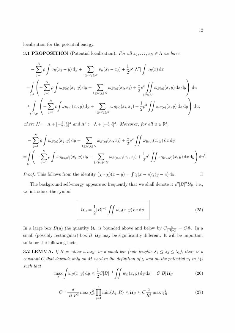
12
localization for the potential energy.
3.1 PROPOSITION (Potential localization). For all x1, . . . , xN ∈ Λ we have
−N∑
j=1
ρ
∫vR(xj − y) dy +
∑
1≤i<j≤NvR(xi − xj) +
1
2ρ2|Λ′′|
∫vR(x) dx
=
∫
R3
−
N∑
j=1
ρ
∫ωB(u)(xj, y) dy +
∑
1≤i<j≤NωB(u)(xi, xj) +
1
2ρ2
∫∫
R3×Λ′′
ωB(u)(x, y) dx dy
du
≥∫
`−1Λ′
−
N∑
j=1
ρ
∫ωB(u)(xj, y) dy +
∑
1≤i<j≤NωB(u)(xi, xj) +
1
2ρ2
∫∫ωB(u)(x, y) dx dy
du,
where Λ′ := Λ + [− `2, `
2]3 and Λ′′ := Λ + [−`, `]3. Moreover, for all u ∈ R3,
−N∑
j=1
ρ
∫ωB(u)(xj, y) dy +
∑
1≤i<j≤NωB(u)(xi, xj) +
1
2ρ2
∫∫ωB(u)(x, y) dx dy
=
∫
R3
(−
N∑
j=1
ρ
∫ωB(u,u′)(xj, y) dy +
∑
1≤i<j≤NωB(u,u′)(xi, xj) +
1
2ρ2
∫∫ωB(u,u′)(x, y) dx dy
)du′.
Proof. This follows from the identity (χ ∗ χ)(x− y) =∫χ(x− u)χ(y − u) du.
The background self-energy appears so frequently that we shall denote it ρ2|B|2 UB, i.e.,
we introduce the symbol
UB =1
2|B|−2
∫∫wB(x, y) dx dy. (25)
In a large box B(u) the quantity UB is bounded above and below by C a|B(u)| = C a
`3. In a
small (possibly rectangular) box B, UB may be significantly different. It will be important
to know the following facts.
3.2 LEMMA. If B is either a large or a small box (side lengths λ1 ≤ λ2 ≤ λ3), there is a
constant C that depends only on M used in the definition of χ and on the potential v1 in (4)
such that
maxx
∫wB(x, y) dy ≤ 1
2C|B|−1
∫∫wB(x, y) dy dx = C|B| UB (26)
C−1 a
|B|R3maxχ2
B
3∏
j=1
minλj, R ≤ UB ≤ Ca
R3maxχ2
B (27)

13
UB ≤ Ca
|B| maxχ2B. (28)
(The scattering length a, which obviously is bounded above and below by constants depending
only on v1, has been included in this inequality for dimensional reasons.)
Proof. The difficult case is a (possibly) rectangular box B = B(u, u′), for the large cubic
boxes B = B(u) the argument is the same just simpler. Recall that for a small box we have
wB(x, y) = χB(x)Ws(x− y)χB(y) and χB(x) = χ1(x1)χ2(x2)χ3(x3), where
χi(xi) = C2/3M ζ(|(xi/`)− ui|)M+1ζ(|(xi/(d`))− u′i|)M+1
for i = 1, 2, 3. The function χi is supported on an interval Ii of length λi corresponding to a
side length of the box. We have 0 < λi ≤ d`. Let I ′i denote the middle third of this interval.
Since ζ is positive and concave on its support, it is a straightforward exercise to check that
infxi∈I′i
χi(xi) ≥ cmaxxi∈Ii
χi(xi) (29)
for i = 1, 2, 3, where c> 0 depends only on M . It is important here that χ is not infinitely
differentiable.
By (4), (23) and the fact that v1 is continuous has compact support and v1(0) > 0 we
may assume that there are constants C1, C2 > 0 (depending only on v1) such that
C1
3∏
i=1
1[−C1R,C1R](xi) ≤ a−1R3Ws(x) ≤ C2
3∏
i=1
1[−C2R,C2R](xi),
where 1I is the characteristic function of the interval I. To prove the inequality (26), it is
therefore enough to prove the 1-dimensional versions:
maxxi∈R
∫χi(xi)1[−C2R,C2R](xi−yi)χi(yi) dyi ≤ Cλ−1
i
∫∫χi(xi)1[−C1R,C1R](xi−yi)χi(yi) dyi dxi,
for i = 1, 2, 3, where C is allowed to depend only on v1 and M . In view of (29) this follows
from
maxxi∈R
∫
Ii
1[−C2R,C2R](xi − yi) dyi ≤ Cλ−1i
∫∫
I′i×I′i1[−C1R,C1R](xi − yi) dyi dxi.
This is obvious since both sides can be estimated above and below by constants times
minλi, R.The lower bound in (27) is proved in a similar fashion. The upper bound in (27) follows
from vR(x) ≤ C aR3 .
For the bound in (28) we note that UB ≤ C|B|−1∫
R3 vR(x) maxχ2B dx ≤ C a
|B| maxχ2B,

14
since ωB(x, y) ≤ CvR(x− y) maxχ2B and that by Condition 1 we have
∫vR(x) dx ≤ Ca.
3.2 Localization of the Kinetic Energy
Let θ be the characteristic function of the cubic box [−1/2, 1/2]3. For u ∈ R3 we denote the
corresponding characteristic function of the box B(u) by θu(x) = θ(x`−1− u). We shall also
use the localization function χu(x) = χ(x`−1 − u) introduced on page 3.
We define the operator Qu to be the orthogonal projection on L2(R3) defined by
Quf = θuf − `−3〈θu|f〉θu. (30)
In other words Quf is a function in L2(R3) that is zero outside the box B(u) and is orthogonal
to the constant functions in the box.
3.3 LEMMA (Abstract kinetic energy localization). Let K : R3 → [0,∞) be a symmetric,
continuous function, which is bounded by a polynomial of degree of most 2M , where M is
the constant introduced in (16). We use it to define an operator on L2(R3) by
T =
∫
R3
QuχuK(−i`∇)χuQu du, (31)
where χu is considered here as a multiplication operator in configuration space. This T is
translation invariant, i.e., a multiplication operator in Fourier space T = F (−i`∇), with
F (p) = (2π)−3K ∗ |χ|2(p)− 2(2π)−3θ(p)χ ∗ (Kχ)(p) + (2π)−3
(∫K|χ|2
)θ(p)2. (32)
In particular, we have F (0) = 0.
Proof. By a simple scaling it is enough to consider ` = 1. This is a straightforward calcula-
tion. Note that Qu has the integral kernel θu(y) [δ(y − x)− 1] θu(x). If we denote by K the
inverse Fourier transform of K, then the integral kernel of the operator QuχuK(−i∇)χuQu
is given by
χu(x)K(x− y)χu(y)− χu(x)[K ∗ χu](x)θu(y)
−θu(x)[K ∗ χu](y)χu(y) + θu(x)〈χu|K(−i∇)χu〉θu(y).
Thus the integral kernel of∫QuχuK(−i∇)χuQu du is given by
([χ ∗ χ]K)(x− y)− 2(χ[K ∗ χ]
)∗ θ(x− y) + (2π)−3
(∫K(p)χ(p)2 dp
)θ ∗ θ(x− y),

15
where we used that∫K(p)χ(p)2 dp is finite by the choice of K. We arrive at the expression
for F by calculating the inverse Fourier transform. The fact that F (0) = 0 follows since
θ(0) =∫θ = 1 and
(2π)3F (0) = 2
(∫Kχ2
)(1− θ(0))2 = 0.
With ` = 1 this lemma is similar to the generalized IMS localization formula
∫
R3
χuK(−i∇)χu du = (2π)−3K ∗ |χ|2,
where K(p) = p2 gives the standard IMS formula since (2π)−3K ∗ |χ|2 = p2 +∫|∇χ|2.
3.4 COROLLARY. With the same notation as above we have that
∫
R3
Qu du = 1− θ(−i`∇)2, (33)
i.e., the operator∫
R3 Qu du is the multiplication operator in Fourier space given by 1− θ(`p)2.
Proof. Simply take K = 1 and χ = θ in the above lemma.
We will use Lemma 3.3 for the function K(p) = ((|p| − s−1)+)2, where s > 0 is the
parameter introduced in Condition 1. Here u+ = maxu, 0 denotes the positive part of u
and we will henceforth write u2+ instead of (u+)2. Note that | − i∇| =
√−∆.
3.5 LEMMA. There is a constant C > 0 (depending on the integer M in the definition
(16) of χ) such that we have the operator inequality
∫Quχu
[√−∆− (s`)−1
]2
+χuQu du ≤ Fs(
√−∆), (34)
where
Fs(|p|) =
(|p| − 1
2(s`)−1)2, if |p| ≥ 5
6(s`)−1
CsM−2p2, if |p| < 56(s`)−1
, (35)
(assuming M ≥ 1).
Proof. We may again by a simple scaling argument assume ` = 1. Since we defined χ in (16)
as an CM0 function, we have for n ≤ 2M and C only depending on M that
∫
|q|>s−1
|q|nχ2(q) dq ≤ s2M−n∫
|q|>s−1
|q|2M χ2(q) dq ≤ Cs2M−n. (36)

16
We use (31) and (32) with K(p) = [|p| − s−1]2+. For the first term in (32) we find
(2π)−3K ∗ χ2(p) ≤ (2π)−3
∫(|p− q| − s−1)2χ2(q) dq
≤ (2π)−3
∫(p2 − 2pq + q2 − 2s−1(|p| − |q|) + s−2)χ2(q) dq
= (|p| − s−1)2 + (2π)−3
∫q2χ2(q) dq + 2(2π)−3s−1
∫|q|χ2(q) dq
≤ (|p| − s−1)2 + Cs−1,
where we have used (2π)−3∫q2χ(q)2 dq =
∫|∇χ|2, that χ2 is even and that s < 1 by
Condition 1. If |p| ≥ 56s−1 we find
(2π)−3K ∗ χ2(p) ≤ (|p| − 1
2s−1)2 − 1
12s−2 + Cs−1.
For the second term in (32) we find since θ ≤ 1 that
|θ(p)χ ∗ (Kχ)(p)| ≤ ||χ||2||Kχ||2 ≤ C
(∫
|q|≥s−1
|q|4|χ(q)|2 dq
)1/2
≤ CsM−2. (37)
For the third term in (32) we have similarly
|θ(p)|2∫K|χ|2 ≤
∫
|q|≥s−1
|q|2χ(q)2 dq ≤ Cs2M−2. (38)
Thus for |p| ≥ 56s−1 and s < 1 we have that the function F in (32) satisfies
F (p) ≤ (|p| − 1
2s−1)2 − 1
12s−2 + Cs−1.
Hence if by Condition 1 s is small enough, we arrive at the first line in (35).
We turn to the proof of the second line in (35). We know that F (0) = 0. Moreover since
F ≥ 0 we must have ∇F (0) = 0. The lemma follows from Taylor’s formula if we can show
that for |p| < 56s−1, we have
|∂i∂jF (p)| ≤ CsM−2. (39)
It is straightforward to see that all second derivatives of K(p) = [|p| − s−1]2+ are bounded
independently of s. For the first term in (32) we thus find for |p| < 56s−1
|∂i∂j(K ∗ χ2)(p)| = |(∂i∂jK) ∗ χ2(p)| ≤ C
∫
|p−q|>s−1
χ(q)2 dq

17
≤ C
∫
|q|>(6s)−1
χ(q)2 dq ≤ Cs2M .
For the second and third term in (32) we use the fact that the numbers
‖θ‖∞, ‖∂iθ‖∞, ‖∂i∂j θ‖∞,∫|χ|2,
∫|∂iχ|2,
∫|∂i∂jχ|2,
for all i, j = 1, 2, 3 are all bounded above by a constant. The same estimates that led to (37)
and (38) then imply (39).
3.6 COROLLARY. If M ≥ 3 we obtain the operator inequality
∫
R3
Qu
χu
[√−∆− 1
2(s`)−1
]2
+χu + b`−2
Qu du ≤ −∆,
provided b is smaller than some universal constant (that we shall not attempt to evaluate).
Proof. We again consider ` = 1. Note that by Corollary 3.4 we have
∫Qu du ≤ β−1 −∆
−∆ + β(40)
for a universal constant 0 < β < 1. We use the previous lemma with s replaced by 2s. We
then find that
∫
R3
Quχu
[√−∆− 1
2s−1]2
+χuQu du+ b
∫
R3
Qu du ≤ F2s(√−∆) + bβ−1 −∆
−∆ + β.
For |p| < (5/12)s−1 Lemma 3.5 gives
F2s(p) + bβ−1 p2
p2 + β≤ Csp2 + bβ−1 p2
p2 + β≤ (Cs+ bβ−2)p2 ≤ p2
for s and b small enough. For |p| ≥ (5/12)s−1 we find from Lemma 3.5 that
F2s(p) + bβ−1 p2
p2 + β≤ (|p| − 1
4s−1)2 + bβ−1 p2
p2 + β≤ p2 − 5
24s−2 +
1
16s−2 + bβ−1 ≤ p2,
for s and b small enough.
This corollary will allow us to localize the kinetic energy to boxes. What will be left as
the kinetic energy in the box B(u) centered at `u, is the operator
Tu = Qu
χu
[√−∆− 1
2(s`)−1
]2
+χu + b`−2
Qu. (41)

18
Note that Tu vanishes on constant functions. The last term in Tu will control the gap in the
kinetic energy, i.e., on functions orthogonal to constants in the box, Tu is bounded below by
at least b`−2.
As explained above, we need to localize even further to smaller boxes whose size is a
factor d 1 smaller than the larger box. In these smaller boxes we also need a term in
the kinetic energy that gives a gap. Unfortunately, the above expression (41) for the kinetic
energy does not immediately allow for such further localization. For this reason we must
introduce a more complicated kinetic energy in the larger box.
We will use
Tu = εT (d`)−2 −∆Nu−∆Nu + (d`)−2
+ b`−2Qu (42)
+Quχu
(1− εT )
[√−∆− 1
2(s`)−1
]2
++ εT
[√−∆− 1
2(ds`)−1
]2
+
χuQu,
where 0 < εT < 1 is a parameter. The operator ∆Nu is the Neumann Laplacian on the box
B(u). As usual ∆ is the Laplacian on R3. Let us be clear about the action of ∆Nu as an
operator on L2(R3). It is the operator associated with the quadratic form
(f,−∆Nu f) =
∫
B(u)
|∇f(x)|2 dx,
which is defined for all functions f ∈ L2(R3) whose restriction to the cube is an H1 function
on the cube, i.e., functions for which the above integral is finite. Note that by the operator
(−∆Nu + (d`)−2)−1 we mean the inverse of −∆Nu + (d`)−2 on the space L2(B(u)) extended
to all of L2(R3) by letting it be 0 on the orthogonal complement, i.e., on functions that live
outside B(u).
Note that if εT = 0 then Tu equals Tu. For the kinetic energy Tu we have a result similar
to Corollary 3.6. For the following theorem we note that on the domain H10 (Λ) we have
∫−∆Nu du = −∆D (43)
in the sense of quadratic forms.
3.7 LEMMA (Large-box kinetic energy localization). If M ≥ 5, and b, d, s, εT > 0 are
smaller than some universal constant then
∫
R3
Tu du ≤ −∆. (44)

19
Proof. As usual we set ` = 1. The first step in the proof is to show that for all d > 0
∫
R3
−∆Nu−∆Nu + d−2
du ≤ −∆
−∆ + d−2. (45)
To show this, we recall that in the sense of quadratic forms∑
u∈Z3 −∆Nu ≤ −∆. Thus
(−∆ + d−2)−1 ≤(∑
u∈Z3
−∆Nu + d−2
)−1
=∑
u∈Z3
(−∆Nu + d−2)−1. (46)
The last equality looks odd, but it is just the identity (⊕
uAu)−1 =
⊕uA−1u applied
to the operators Au = −∆Nu + d−21L2(B(u)) acting on L2(B(u)) recalling that L2(R3) =⊕
u∈Z3 L2(B(u)).
Since 1− d−2(−∆ + d−2)−1 = −∆(−∆ + d−2)−1, it follows from (46) that
∑
u∈Z3
−∆Nu−∆Nu + d−2
≤ −∆
−∆ + d−2. (47)
This will also hold if we replace the sum over Z3 by a sum over v + Z3 for any v ∈ [0, 1]3.
An integration over v ∈ [0, 1]3 gives (45).
The second step is to observe that from Lemma 3.5, e.g., with M ≥ 5 we find that
∫Quχu
[(1− εT )
[√−∆− 1
2s−1]2
++ εT
[√−∆− 1
2(ds)−1
]2
+
]χuQu du
≤ (1− εT )[√−∆− 1
4s−1]2
++ εT
[√−∆− 1
4(ds)−1
]2
++ Cs
−∆
−∆ + β
for some universal constant C and where β is the same constant as in (40). The proof is
completed using (40) and observing that if s, b, d, εT are all smaller than some universal
constant then for all p ∈ R3
(bβ−1 + Cs)p2
p2 + β+ εTd
−2 p2
p2 + d−2+ (1− εT )
[|p| − 1
4s−1]2
++ εT
[|p| − 1
4(ds)−1
]2+≤ p2.
We now discuss the further localization into smaller boxes of relative size d 1. As
in the previous subsection we index these boxes by a parameter u′ ∈ R3. The small box is
B(u′) = d`Γu′ = d`u′+ [−d`/2, d`/2]3, whose center is at d`u′. We denote the corresponding

20
characteristic function and localization function by
θu′(x) = θ((x/d`)− u′), χu′(x) = χ((x/d`)− u′).
The corresponding orthogonal projection onto functions orthogonal to constants in L2(B(u′))
is Qu′ given by
Qu′f = θu′f − (d`)−3〈θu′|f〉θu′ .
When localizing in to the smaller boxes, we are forced to consider the situation of overlap
between the large boxes and small boxes, i.e., B(u, u′) = B(u) ∩ B(u′). The corresponding
characteristic function is θuθu′ , the corresponding localization function is χuχu′ , and the
corresponding orthogonal projection is
Quu′f = θuθu′f − |B(u, u′)|−1〈θuθu′ |f〉θuθu′ .
Our first result is that when we localize the large box kinetic energy Tu into smaller boxes
we will get a gap in the localized energy spectrum. This is a consequence of the next result.
3.8 LEMMA. With Quu′ as defined above and β = 1 + π−2 we have for all d > 0
∫Quu′ du
′ ≤ β−∆Nu
−∆Nu + (d`)−2. (48)
Proof. It is enough to consider ` = 1. Let −∆Nuu′ denote the Neumann Laplacian in the box
B(u, u′). Observe that since B(u, u′) ⊆ B(u′), the Neumann Laplacian −∆Nuu′ has a gap of
at least π2d−2, i.e., −∆Nuu′ ≥ π2d−2Quu′ . Thus
Quu′ ≤ β−∆Nuu′
−∆Nuu′ + d−2.
The same argument that led to (45) gives
∫ −∆Nuu′−∆Nuu′ + d−2
du′ ≤ −∆Nu−∆Nu + d−2
,
which concludes the proof of the lemma.
This lemma shows that the first term in (42), after localization, leads to a gap in the
small boxes. The full kinetic energy localization is given in the next lemma.
3.9 LEMMA (Small-box kinetic energy localization). Let Tu be the kinetic energy given in

21
(42) in terms of the parameters s, d, εT and the constant b. Let
Tuu′ = εT b(d`)−2Quu′ +Quu′χuχu′
[√−∆− (ds`)−1
]2
+χu′χuQuu′ . (49)
Our assertion is that if (s−2 + d−3)(ds)−2sM ≤ δ, then, for all 0 < εT < 1,
Tu−b
2`−2Qu ≥
∫Tuu′ du′,
provided that b and d are smaller than some universal constant. The first term in (49) yields
a gap above zero of size εT b(d`)−2 in the spectrum of Tuu′, which we will refer to as the
Neumann gap.
Proof. We again take ` = 1. The integral over the first term in Tuu′ is bounded above by
the first term in Tu by Lemma 3.8 if b is smaller than the constant β−1 in that lemma. We
concentrate on the second term in Tuu′ . By a unitary transformation (x 7→ x/d and p 7→ pd)
of the result in Lemma 3.5 we obtain that
∫Qu′χu′
[√−∆− (ds)−1
]2
+χu′Qu′ du
′ ≤ d−2Fs(d√−∆)
≤ (1− εT )[√−∆− 1
2s−1]2
++ εT
[√−∆− 1
2(ds)−1
]2
++ C(ds)−2sM−2,
where the function Fs is given in (35) and we used that[√−∆− 1
2(ds)−1
]2+≤[√−∆− 1
2s−1]2
+.
Thus the proof would be complete if the operator appearing as the integrand in the second
term in Tuu′ would have been, instead,
QuχuQu′χu′[√−∆− (ds)−1
]2
+χu′Qu′χuQu.
We will estimate the difference between these operators, which is
D = QuχuQu′χu′[√−∆− (ds)−1
]2
+χu′Qu′χuQu
−Quu′χuχu′[√−∆− (ds)−1
]2
+χu′χuQuu′
= Qu
(χuQu′ −Quu′χu
)χu′[√−∆− (ds)−1
]2
+χu′Qu′χuQu
+Quu′χuχu′[√−∆− (ds)−1
]2
+χu′(Qu′χu − χuQuu′
)Qu,

22
where we have used that QuQuu′ = Quu′ . We observe that (using Dirac notation)
(χuQu′ −Quu′χu
)χu′ = χuθu′χu′ − d−3χu|θu′〉〈θu′|χu′ − θuθu′χuχu′
+ |B(u, u′)|−1|θuθu′〉〈θuθu′ |χuχu′= |B(u, u′)|−1|θuθu′〉〈χuχu′ | − d−3|χuθu′〉〈χu′ |,
exploiting the facts that θu′χu′ = χu′ and θuχu = χu. It is now simple to estimate the
operator norm of D
‖D‖ ≤ C
∥∥∥∥(χuQu′ −Quu′χu
)χu′[√−∆− (ds)−1
]2
+
∥∥∥∥
≤ C|B(u, u′)|−1/2
(∫
|p|>(ds)−1
|p|4 |χuχu′(p)|2 dp
)1/2
+ Cd−3/2
(∫
|p|>(ds)−1
|p|4 |χu′(p)|2 dp
)1/2
≤ C(ds)M−2|B(u, u′)|−1/2〈χuχu′|(−∆)Mχuχu′〉1/2 + C(ds)M−2d−3/2〈χu′|(−∆)M χu′〉1/2
≤ C(ds)M−2d−M ≤ C(ds)−2sM .
Hence D = QuDQu ≥ −C(ds)−2sMQu and
∫Quu′χuχu′
[√−∆− (ds)−1
]2
+χu′χuQuu′ du
′
=
∫QuχuQu′χu′
[√−∆− (ds)−1
]2
+χu′Qu′χuQu du′ −
∫
u′|B(u)∩B(u′) 6=∅D du′
≤ Quχu
((1− εT )
[√−∆− 1
2s−1]2
++ εT
[√−∆− 1
2(ds)−1
]2
+
)χuQu
+C(s−2 + d−3)(ds)−2sMQu.
We have here used the fact that the volume of u′|B(u)∩B(u′) 6= ∅ is bounded by Cd−3.
We shall throughout the rest of the paper assume that the conditions in Lemmas 3.7 and
3.9 are satisfied.
CONDITION 2: In terms of the integer M appearing in the definition (16) of χ (and
which will be specified later to be ≥ 5) we have
0 < εT < δ, and (s−2 + d−3)(ds)−2sM ≤ δ, (50)
where δ is the quantity which we introduced in Condition 1 to ensure adequate smallness of

23
relevant parameters.
3.3 Localization of the Total Energy
We define the localized Hamiltonian, Hu, in a “large” box B(u) to be
Hu =N∑
i=1
(1− ε0)Tu,i − ρ
∫wB(u)(xi, y) dy
+
∑
1≤i<j≤NwB(u)(xi, xj)
+1
2ρ2
∫∫wB(u)(x, y) dx dy, (51)
where 0 < ε0 < 1/2 is a parameter to be determined later. The subscript i, as usual,
refers to the ith particle. Recall that Tu was defined in (42) and wB(u) was defined in (24).
The Hamiltonian Hu is defined as a quadratic form on permutation-symmetric functions in
H10 (ΛN).
The localized Hamiltonian in a “small” box B(u, u′) is
Huu′ =N∑
i=1
(1− ε0)Tuu′,i − ρ
∫wB(u,u′)(xi, y) dy
+
∑
1≤i<j≤NwB(u,u′)(xi, xj)
+1
2ρ2
∫∫wB(u,u′)(x, y) dx dy, (52)
where wB(u,u′) was defined in (24) and Tuu′ was defined in (49). The results of Proposition 3.1,
(43) and Lemmas 3.7 and 3.9 can be combined to give our final localization estimate.
3.10 THEOREM (Main localization inequalities).
If Condition 2 is satisfied, we have for all 0 ≤ ε0 ≤ 1/2 that
Hρ,N ≥∫
`−1Λ′
(−ε0∆Nu +Hu
)du, and, for all u ∈ R3, Hu−
b
2`−2Qu ≥
∫
R3
Huu′ du′. (53)
We introduce the notation that
HB =
Hu, if B = B(u)
Huu′ , if B = B(u, u′)(54)
and
TB =
(1− ε0)Tu, if B = B(u)
(1− ε0)Tuu′ , if B = B(u, u′).(55)

24
The reason for the above (1− ε0) term is that we still need some kinetic energy in the end
of this paper when we want to apply Lemma 6.6. With the corresponding notations for wB
in (24) the box Hamiltonian can be written
HB =N∑
i=1
(TB,i − ρ
∫wB(xi, y) dy
)+
∑
1≤i<j≤NwB(xi, xj) +
1
2ρ2
∫∫wB(x, y) dx dy. (56)
4 Energy in a Single Box
In this section we will study the energy in a single box B, i.e., the ground state energy of
the Hamiltonian HB. We denote by PB the orthogonal projection onto the characteristic
function of B and by QB the projection orthogonal to constant functions in B, i.e., such
that PB + QB = 1B is the projection onto the subspace of functions supported on B. We
define the operators
n =N∑
i=1
1B,i, n0 =N∑
i=1
PB,i, n+ =N∑
i=1
QB,i.
Here n represents the number of particles in the box B, n0 the number of particles in the
constant function, which we will refer to as the condensate particles, and n+ the number
of particles not in the condensate, which we will refer to as the excited particles. We have
n = n+ + n0.
The particle number operator n commutes with the box operator HB, but n+ and n0 do
not commute with HB. In our discussion below we may assume that n is a parameter, i.e.,
we restrict to eigenspaces for the operator n. We shall not distinguish between the operator
n and its eigenvalues.
We give a simple a priori bound on n+, which will be improved later.
4.1 LEMMA (Simple bound on the ground state energy of HB and on n+).
The ground state energy EB of HB satisfies
0 > EB ≥ −Cnρ|B|UB (57)
with UB given in (25). Moreover, in any state for which the expectation value
〈HB〉 ≤ 12ρ2∫∫wB(x, y) dx dy = ρ2|B|2UB we have
〈n+〉 ≤ C(1− ε0)−1ε−1T b−1ρa(d`)2nmaxχ2
B, (58)

25
if B = B(u, u′).
Proof. The upper bound on EB follows by using a trial state in which all particles are in the
condensate, i.e., an eigenstate of n+ with eigenvalue 0. If there are n particles, we find that
the expectation value in this state is
〈HB〉 =1
2
[(n− ρ|B|)2 − n
]|B|−2
∫∫wB(x, y) dx dy.
We can choose n ≥ 1 such that |n− ρ|B|| < 1. Hence 〈HB〉 < 0 and thus the ground state
energy of HB is negative. The lower bound on EB follows immediately from (26) since TBand wB are non-negative.
If a state satisfies 〈HB〉 ≤ 12ρ2∫∫
wB(x, y) dx dy, we have
0 ≥N∑
i=1
⟨TB,i − ρ
∫wB(xi, y) dy
⟩≥ (1− ε0)εT b(d`)
−2〈n+〉 − Cρanmaxχ2B,
where we have used (49) and that maxx
∫ωB(x, y) dy ≤ Camaxχ2
B as we have seen in Lemma
3.2. This gives the second estimate in the lemma.
4.1 The Negligible (Non-Quadratic) Parts of the Potential
We treat the potential energy terms in HB according to how many excited particles they
involve. We write 1B = PB + QB and we expand and classify the terms according to the
number of Q-factors, no-Q, 1-Q, . . . , 4-Q. In the following we will simply write PB = P and
QB = Q.no-Q terms:
Q0 := −∑
i
ρPi
∫wB(xi, y) dyPi +
∑
i<j
PiPjwB(xi, xj)PiPj +1
2ρ2
∫∫wB(x, y) dx dy
=[(n0 − ρ|B|)2 − n0
]UB =
[(n− ρ|B|)2 − 2(n− ρ|B|)n+ + n2
+ − n0
]UB, (59)
where we have used the notation (25).
1-Q terms:
Q1 :=∑
i,j
PiPjwB(xi, xj)QiPj −∑
i
ρPi
∫wB(xi, y) dyQi + h.c.

26
=∑
i
Pi
∫wB(xi, y) dyQi(n0|B|−1 − ρ) + h.c.
= Q′1 +Q′′1, (60)
where
Q′1 = (n− ρ|B|)|B|−1
(∑
i
Pi
∫wB(xi, y) dyQi +
∑
i
Qi
∫wB(xi, y) dyPi
)(61)
and
Q′′1 = −|B|−1∑
i
Pi
∫wB(xi, y) dyQin+ − |B|−1
∑
i
n+Qi
∫wB(xi, y) dyPi. (62)
4.2 LEMMA (Estimates on Q1 ). For all ε′1, ε′′1> 0
Q′1 ≥− |n− ρ|B||(ε′1n0 + ε′−11 Cn+)UB
and
Q′′1 ≥− (ε′′1(n+ + 1)n0 + Cε′′−11 n2
+)UB.
Proof. We prove first the bound on Q′′1. We have
Q′′1 = −√n+ + 1
∑
i
Pi
∫wB(xi, y) dyQi
√n+ |B|−1 + h.c.
since for any self-adjoint operator A we get∑
i PiAiQin+ = (n+ + 1)∑
i PiAiQi and hence∑
i PiAiQi√n+ =
√n+ + 1
∑i PiAiQi.
Since wB ≥ 0, we obtain from a Schwarz inequality and Lemma 3.2 that
Q′′1 ≥ −(ε′′1(n+ + 1)
∑
i
Pi + Cε′′−11 n+
∑
i
Qi
)UB.
The estimate on Q′1 follows by applying a similar Schwarz inequality.
2-Q terms: There are two kinds of 2-Q terms. There are terms which contribute to the
energy to the order of interest. They will primarily be treated together with the quadratic
Hamiltonian later on. The remaining 2-Q terms are negligible error terms that we will
estimate here.

27
The 2-Q terms that will later appear in the quadratic Hamiltonian are
Q′2 :=∑
i,j
PiQjwB(xi, xj)PjQi +∑
i<j
(QiQjwB(xi, xj)PjPi + PjPiwB(xi, xj)QiQj). (63)
We shall however give an a priori estimate on these terms already now. This estimate will
be used in Case II in the proof of Lemma 5.2. Using the estimate 0 ≤ wB ≤ CaR−3 maxχ2B
and the Schwarz inequality twice gives that
Q′2 ≥ −∑
i,j
PiQjwB(xi, xj)PiQj −∑
i<j
(2QiQjwB(xi, xj)QjQi +
1
2PjPiwB(xi, xj)PiPj
)
≥ −n0|B|−1∑
i
Qi
∫wB(xi, y) dyQi − Cn2
+aR−3 maxχ2
B −1
2
∑
i<j
PjPiwB(xi, xj)PiPj
≥ −Cnn+ UB − Cn2+aR
−3 maxχ2B −
1
2n2 UB. (64)
In the last inequality we have used that∑i
Qi
∫ωB(xi, y) dyQi ≤ C|B|UBn+ by (26) since
∑i
Qi
∫ωB(xi, y) dyQi commutes with n+. The negligible 2-Q terms are estimated in the
same way
Q′′2 := −∑
i
ρQi
∫wB(xi, y) dyQi +
∑
i,j
QiPjwB(xi, xj)PjQi
= (n0 − ρ|B|)|B|−1∑
i
Qi
∫wB(xi, y) dyQi (65)
= (n− ρ|B| − n+)|B|−1∑
i
Qi
∫wB(xi, y) dyQi ≥ −C
([ ρ|B| − n ]+n+ + n2
+
)UB.
3-Q terms: For all ε3 > 0
Q3 :=∑
i,j
PjQiwB(xi, xj)QiQj + h.c.
≥ −∑
i 6=j
(2ε−1
3 PjQiwB(xi, xj)QiPj +ε3
2QjQiwB(xi, xj)QiQj
)
≥ −Cε−13 nn+ UB − ε3
∑
i<j
QjQiwB(xi, xj)QiQj. (66)
The first inequality uses a Schwarz inequality, while the second inequality uses Lemma 3.2
and the fact that n0 ≤ n. Note that the above estimates are given as lower bounds, but that
we of course also could have stated them as two-sided bounds. The last term above can be

28
absorbed into the positive 4-Q term if ε3 ≤ 1. We will do this initially, but at a later stage
in the proof we have to control the first term in (66) by choosing ε3 1. At that time we
will have good control over the number of excited particles, n+, in the large box. The second
term in (66) will then be controlled by applying Lemma 6.6, where we apply the kinetic
energy term∑i
− ε0∆Nu,i that we have saved in Theorem 3.10 for exactly this purpose.
4-Q term: This is the positive term
Q4 :=∑
i<j
QjQiwB(xi, xj)QiQj (67)
and for a lower bound it can be ignored or used to control other errors. We will only need
an estimate on the 4-Q term in a large box B = B(u) as explained above.
4.2 The Quadratic Hamiltonian
We can write the box Hamiltonian as
HB =N∑
i=1
TB,i +Q0 +Q′1 +Q′′1 +Q′2 +Q′′2 +Q3 +Q4. (68)
We have estimated all terms except the quadratic part∑N
i=1 TB,i +Q′2. We first consider the
kinetic energy.
For B = B(u), i.e., a large box we have from (42) and (55) that
TB = (1− ε0)εT (d`)−2 −∆Nu−∆Nu + (d`)−2
+ (1− ε0)b`−2Q+QχBτB(−∆)χBQ (69)
with
τB(k2) = (1− ε0)(1− εT )[|k| − 1
2(s`)−1
]2+
+ (1− ε0)εT[|k| − 1
2(ds`)−1
]2+. (70)
For B = B(u, u′), i.e., a small box we have from (49) and (55) that
TB = (1− ε0)εT b(d`)−2Q+QχBτB(−∆)χBQ (71)
with
τB(k2) = (1− ε0)[|k| − (ds`)−1
]2+. (72)

29
The interesting part of TB is the term of form QχBτB(−∆)χBQ. The other terms, which are
positive, are only used to control errors. We put them aside for the moment and define the
quadratic Hamiltonian
HQuad =N∑
i=1
(QχBτB(−∆)χBQ)i +Q′2. (73)
At the end of this paper it will be useful to treat the term Q′1 together with HQuad.
To handle HQuad, we use the formalism of second quantization. For all k ∈ R3 we define the
operator
bk = a∗0a(Q(eikxχB)), (74)
where a(Q(eikxχB)) is the operator that annihilates an exited particle in the state given by the
function Q(eikxχB) ∈ L2(B), and a0 is the operator that creates a particle in the condensate.
These two operators commute. Note that bk is a bounded operator when restricted to a
subspace of finite n. Its adjoint is
b∗k = a(Q(eikxχB))∗a0. (75)
Since a∗0 commutes with a(Q(eikxχB)), we have the commutation relations
[bk, bk′ ] = 0, [bk, b∗k′ ] = a∗0a0
⟨Q(eikxχB)
∣∣Q(eik′xχB)
⟩− a(Q(eik
′xχB))∗a(Q(eikxχB)), (76)
for all k, k′ ∈ R3. In particular,
[bk, b∗k] ≤ a∗0a0
∫χ2B = n0
∫χ2B. (77)
Moreover,
b∗kbk ≤ n+(n0 + 1)
∫χ2B. (78)
The term QχBτB(−∆)χBQ and its second quantization can be written
QχBτB(−∆)χBQ = (2π)−3
∫
R3
τB(k2)∣∣Q(χBe
ikx)⟩ ⟨Q(χBe
ikx)∣∣ dk
2nd quant−→ (2π)−3
∫
R3
τB(k2)a(Q(χBeikx))∗a(Q(χBe
ikx)) dk
≥ (2π)−3
∫
R3
τB(k2)a(Q(χBeikx))∗
a0a∗0
na(Q(χBe
ikx)) dk
= (2π)−3n−1
∫
R3
τB(k2)b∗kbk dk. (79)

30
Here we used that bkψ = 0 if ψ is in the condensate allowing us to assume that n+ ≥ 1 such
that in fact a0a∗0 ≤ n. Likewise we may write
Q′2 =1
2(2π)−3|B|−1
∫W (k)
(b∗kbk + b∗−kb−k + b∗kb
∗−k + bkb−k
)dk
−(2π)−3|B|−1
∫W (k)a(Q(χBe
ikx))∗a(Q(χBeikx)) dk (80)
and
Q′1 = (n− ρ|B|)(2π)−3|B|−3/2
∫W (k)
(χB(k)bk + χB(k)b∗k
)dk. (81)
The last term in Q′2 may be written
(2π)−3|B|−1
∫W (k)a(Q(χBe
ikx))∗a(Q(χBeikx)) dk =
N∑
i=1
QiZiQi, (82)
where Z is the operator with integral kernel
kZ(x, y) = |B|−1χB(x)W (x− y)χB(y). (83)
4.3 LEMMA. The operator Z on L2(R3) with integral kernel (83) satisfies the bound
‖Z‖ ≤ CaminR−3, |B|−1maxχ2B.
In particular, if B = B(u), we have
||Z|| ≤ Ca|B|−1. (84)
Proof. It is clear that
‖Z‖ ≤ |B|−1 maxχ2B
∫W ≤ C|B|−1 maxχ2
B
∫v1 ≤ Ca|B|−1 maxχ2
B.
If we use that the Hilbert-Schmidt norm is greater than the operator norm, ‖Z‖ ≤ ‖Z‖HS,
we find
‖Z‖ ≤ |B|−1
(∫∫χB(x)2W (x− y)2χB(y)2 dx dy
)1/2
≤ |B|−1 maxW
∫χ2B ≤ CaR−3 maxχ2
B.

31
Combining the above lemma with (73), (79), (80), and (81), we arrive at the following
result.
4.4 LEMMA. For all σ ∈ R we have the estimate
HQuad + σQ′1 ≥1
2(2π)−3
∫
R3
hσ(k) dk − Cn+aminR−3, |B|−1maxχ2B, (85)
where
hσ(k) = n−1τB(k2)(b∗kbk + b∗−kb−k) + W (k)|B|−1(b∗kbk + b∗−kb−k + b∗kb∗−k + bkb−k)
+ σ(n− ρ|B|)W (k)|B|−3/2(χB(k)(bk + b∗−k) + χB(k)(b∗k + b−k)
).
(If n = 0 then hσ(k) = 0.)
Note that if we for the smallest side length of a small box have λ1 ≥ ρ−13 , then
Cn+aminR−3, |B|−1maxχ2B ≤ Cn+ρa, which is smaller than the Neumann gap on the
small box.
We shall now give an estimate on hσ(k), which is based on a simple version of Bogolubov’s
treatment of quadratic Hamiltonians. This estimate requires, however, assumptions which
will not be fulfilled in all our situations. The following result is Theorem 6.3 in [13] except
that we state it here a bit more generally. In the original [13] it was required A ≥ B > 0, but
this is not needed. The operators b± can, for example, be any commuting pair of bounded
operators (the case we will use here) or they can be annihilation operators in Fock space
(the original Bogolubov case).
4.5 THEOREM (Simple case of Bogolubov’s method).
For arbitrary A,B ∈ R satisfying A > 0, −A < B ≤ A and κ ∈ C we have the operator
inequality
A(b∗+b+ + b∗−b−) + B(b∗+b∗− + b+b−) + κ(b∗+ + b−) + κ(b+ + b∗−)
≥ −12(A−
√A2 − B2)([b+, b
∗+] + [b−, b
∗−])− 2|κ|2
A+ B ,
where b± are operators on a Hilbert space satisfying [b+, b−] = 0.
Proof. The proof is essentially the same as in the original [13]. We may complete the square
A(b∗+b+ + b∗−b−) + B(b∗+b∗− + b+b−) + κ(b∗+ + b−) + κ(b+ + b∗−)
= D(b∗+ + αb− + a)(b+ + αb∗− + a) +D(b∗− + αb+ + a)(b− + αb∗+ + a)
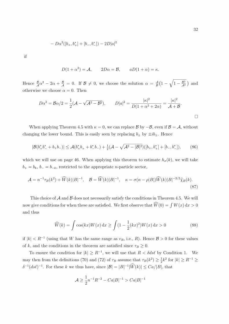
32
−Dα2([b+, b∗+] + [b−, b
∗−])− 2D|a|2
if
D(1 + α2) = A, 2Dα = B, aD(1 + α) = κ.
Hence BAα
2 − 2α + BA = 0. If B 6= 0, we choose the solution α = A
B(1 −
√1− B2
A2
)and
otherwise we choose α = 0. Then
Dα2 = Bα/2 =1
2(A−
√A2 − B2), D|a|2 =
|κ|2D(1 + α2 + 2α)
=|κ|2A+ B .
When applying Theorem 4.5 with κ = 0, we can replace B by −B, even if B = A, without
changing the lower bound. This is easily seen by replacing b± by ±ib±. Hence
|B(b∗+b∗− + b+b−)| ≤ A(b∗+b+ + b∗−b−) + 1
2(A−
√A2 − |B|2)([b+, b
∗+] + [b−, b
∗−]), (86)
which we will use on page 46. When applying this theorem to estimate hσ(k), we will take
b+ = bk, b− = b−k, restricted to the appropriate n-particle sector,
A = n−1τB(k2) + W (k)|B|−1, B = W (k)|B|−1, κ = σ(n− ρ|B|)W (k)|B|−3/2χB(k).
(87)
This choice ofA and B does not necessarily satisfy the conditions in Theorem 4.5. We will
now give conditions for when these are satisfied. We first observe that W (0) =∫W (x) dx > 0
and thus
W (k) =
∫cos(kx)W (x) dx ≥
∫(1− 1
2(kx)2)W (x) dx > 0 (88)
if |k| < R−1 (using that W has the same range as vR, i.e., R). Hence B > 0 for these values
of k, and the conditions in the theorem are satisfied since τB ≥ 0.
To ensure the condition for |k| ≥ R−1, we will use that R < δds` by Condition 1. We
may then from the definitions (70) and (72) of τB assume that τB(k2) ≥ 12k2 for |k| ≥ R−1 ≥
δ−1(ds`)−1. For these k we thus have, since |B| = |B|−1|W (k)| ≤ Ca/|B|, that
A ≥ 1
2n−1R−2 − Ca|B|−1 > Ca|B|−1

33
if n|B|−1 ≤ c(aR2)−1 for c sufficiently small (depending only on v1). This implies that A is
positive and that A ≥ |B|.In this case we are therefore allowed to use Theorem 4.5 to bound hσ(k) and in fact we may
assume that A + B ≥ 2|B| if c is sufficiently small. When the condition n|B|−1 ≤ c(aR2)−1
can not be satisfied, which only happens on page 37 in Case 2 of the proof of Lemma 5.2,
we use (64) instead.
4.6 LEMMA. There exists c > 0 (depending only on v1) such that if n|B|−1 ≤ c(aR2)−1
then for all k ∈ R3
hσ(k) ≥−(n−1τB(k2) + |B|−1W (k)−
√n−2τB(k2)2 + 2n−1|B|−1τB(k2)W (k)
)n0
∫χ2B
− σ2(n− ρ|B|)2|B|−2|χB(k)|2W (k)− Cσ2(n− ρ|B|)2|B|−2|χB(k)|2|W (k)|1|k|≥R−1(k),
(89)
where M is the integer in the definition (16) of χ.
Proof. As we just saw, we are in a situation where we can use Bogolubov’s method from
Theorem 4.5 with A+ B ≥ 2|B|. This gives the estimate
2|κ|2(A+ B)−1 ≤ σ2(n− ρ|B|)2|B|−2|χB(k)|2|W (k)|.
Now (89) follows, since we have already seen in (77) that [bk, b∗k] ≤ n0
∫χ2B and in (88) that
W (k) > 0 for |k| < R−1.
We shall primarily use the above lemma with σ = 0. On page 49 we will also use it with
σ = 1 on the large box and then the second to last term in (89) will, after integration over
k, give
−1
2(2π)−3σ2(n− ρ|B|)2|B|−2
∫|χB(k)|2W (k) dk = −σ2(n− ρ|B|)2UB,
using the notation (25), and hence exactly cancel the first positive term in (59). Recalling
that χu(x) = χ(x`−1 − u) and using (36) together with the estimate |W (k)| ≤ Ca, we see
that the last term in (89), after integration over k, will be bounded by
Cσ2|B|−1a(n− ρ|B|)2(R/`)2M
∫|k|2M |χ(k)|2 dk ≤ Cσ2|B|−1a(n− ρ|B|)2(R/`)2M . (90)

34
We have by Condition 1 that R ` and this will be enough to control the last term in (89)
if M is sufficiently large.
5 A Priori Bounds on the Non-Quadratic Part of the
Hamiltonian and on n
We shall eventually prove that the lowest energy of the box Hamiltonian HB will be achieved
when the particle number n is close in an appropriate sense to ρ|B|. In this subsection we will
give a much weaker a priori bound on n. The main difficulty lies in treating the (possibly)
rectangular small boxes B(u, u′) of side lengths λ1 ≤ λ2 ≤ λ3 ≤ d`.
5.1 LEMMA (Estimates on the non-quadratic part of HB).
If B is a small box, we have
HB −HQuad ≥ (1− ε0)εT b(d`)−2n+ +
[7
8|n− ρ|B||2 − C|n− ρ|B||n+ − Cn− Cnn+
]UB
(91)
and if B is a large box, we have
HB −HQuad ≥ (1− ε0)b`−2n+ +
[7
8|n− ρ|B||2 − C|n− ρ|B||n+ − Cn− Cnn+
]UB, (92)
where b and b are the universal constants appearing in (42) and (49).
Proof. We use estimate (59), Lemma 4.2 (with ε′1 = |n−ρB|8n
), (64), (65), (66), (67), the
respective Neumann gaps and the fact that n+ ≤ n to obtain (91) and (92).
The constant 78
is of course not optimal and has been chosen for notational purposes only.
To prove the next lemma, we would like to use that n+ is much smaller than n. This follows
from Lemma 4.1 in view of the following Condition, which we henceforth assume to hold.
CONDITION 3: We require that
(√ρad`)2 ≤ cT εT , (93)
where cT is a small but universal constant.
5.2 LEMMA (A priori bound on n).
There is a constant C0 > 0 such that for any state with fixed particle number n on a small

35
box satisfying 〈ψ|HB|ψ〉 ≤ 0, we have
n ≤ C0|B|max
3∏
j=1
(minλj, R)−1, ρ
. (94)
Proof. Assume C0 ≥ 2 and set
KB = C0|B|max
3∏
j=1
(minλj, R)−1, ρ
.
Then KB ≥ C0|B|∏3
j=1 λ−1j = C0 ≥ 2. If n ≥ KB, let m be the integer part of nK−1
B . We
can then divide the particles into m groups of particles consisting of n1, . . . , nm particles
where∑m
j=1 nj = n and
1
2KB ≤ nj ≤ 2KB, j = 1, . . . ,m. (95)
We now use that the interaction ωB between the particles is non-negative and thereby
get the following lower bound if we ignore the interactions between the groups and correct
for the background self-energy term
〈ψ|HB|ψ〉 − ρ2|B|2UB ≥ m inf〈ψ′|HB|ψ′〉 − ρ2|B|2UB
∣∣∣ψ′ has n′ particles in B,1
2KB ≤ n′ ≤ 2KB
.
Our aim is to prove that if C0 is large enough, then
〈ψ′|HB|ψ′〉 − ρ2|B|2UB ≥ 0
if ψ′ has particle number n′ satisfying KB/2 ≤ n′ ≤ 2KB. We have
ρ2|B|2 ≤ C−20 K2
B ≤ 4C−20 n′2. (96)
Using that n′ ≥ C0
2, we have n′ ≤ 2
C0n′2 and |n′ − ρ|B|| ≥ (1− 2
C0)n′. With n′+ = 〈ψ′ | n+ | ψ′〉
we obtain from Lemma 4.1, Lemma 5.1 and (96) that
〈ψ′|HB −HQuad|ψ′〉 − ρ2|B|2UB ≥ (1− ε0)εT b(d`)−2n′+ +
3
4n′2UB, (97)
if C0 is sufficiently large and δ sufficiently small. It remains to bound HQuad. To do this,
we differentiate between whether or not we are allowed to apply Bogolubov’s method. With
c > 0 being the constant in Lemma 4.6 which will allow us to use the Bogolubov bound, we

36
first treat boxes where the side length and the parameter R are not too small in the sense
that
Case I: KB < (c/2)|B|(aR2)−1
Here we are allowed to use Bogolubov’s method, i.e., Lemma 4.6. Combining (A.6), (A.7),
(A.8) and (A.15), we get
〈ψ′|HQuad|ψ′〉 ≥1
2(2π)−3
∫
R3
h0(k) dk − Cn′+aminR−3, |B|−1
maxχ2
B
≥ −Cn′a(ds`)−3 maxχ2B − Cn′
n′
|B|aa
Rmaxχ2
B − Cn′n′2
|B|2a3Rmaxχ2
B − Cn′a
R3maxχ2
B
≥ −Cn′ aR3
maxχ2B − Cn′
KB
|B|aa
Rmaxχ2
B − Cn′K2B
|B|2a3Rmaxχ2
B
≥ −Cn′ aR3
maxχ2B. (98)
Using the lower bound in (27) together with (95) and (97), we have that
〈ψ′|HB|ψ′〉 − ρ2|B|2UB ≥ Cn′2UB − Cn′a
R3maxχ2
B
= Cn′UB(n′ − CU−1B
a
R3maxχ2
B)
≥ Cn′UB(n′ − CC−10 n′),
which is positive if C0 is sufficiently large.
Case II: KB ≥ (c/2)|B|(aR2)−1
By Condition 1 and the Case II assumption we have
KB
|B| = C0
3∏
j=1
(minλj, R)−1 ≥ c
2(aR2)−1. (99)
Since R, λj ≤ d` we have |B| ≤ Ca(d`)2 such that maxχ2B ≤ C
(ad`
)4(M+1)by (19). By
Lemma 4.1 and Condition 3, we have n+ ≤ CcTnmaxχ2B. From the lower bound in (27) we
get
Cn′2+a
R3maxχ2
B ≤ CcTn′2 a
R3maxχ4
B
≤ CcTn′2|B|
3∏
j=1
(minλj, R)−1 maxχ2B UB
≤ CcTn′2(d`
R
)3 ( ad`
)4(M+1)
UB.

37
Together with equation (97) and the estimate
〈ψ′|HQuad|ψ′〉 ≥ 〈ψ′|Q′2|ψ′〉 ≥ −5
8n′2 UB − Cn2
+
a
R3maxχ2
B,
which follows from (64), this yields
〈ψ′|HB|ψ′〉 − ρ2|B|2 UB ≥1
8n′2 UB − Cn′2+aR−3 maxχ2
B ≥ 0,
provided δ is sufficiently small.
When applying the above lemma, we will assume that the box B = B(u, u′) has ei-
ther smallest side length λ1 ≤ ρ−13 or λ1 > ρ−
13 . Note that if λ1 > ρ−
13 , we get n ≤
C0|B|max R−3, ρ and may apply Lemma 4.6.

38
5.1 A Priori Bounds on the Energy in the Small Box
Small boxes at the boundary of the large box may be arbitrarily small. We first consider
the case of boxes which are so small that Bogolubov’s method can not be applied. By the
lemma below these boxes only contribute to e0(ρ) by an amount, which is of lower order
than the LHY-term.
5.3 LEMMA (Lower bound on the energy on small boxes with λ1 ≤ ρ−13 ).
Let B = B(u, u′) be a small box with smallest side length λ1 ≤ ρ−13 . Then
〈HB〉 ≥ −C|B|maxρ,R−3
a
R3
(ρ−
13
d`
)4M+2
, (100)
where M is the integer in the definition (16) of χ. For all u ∈ R3
∫
λ1(B(u,u′))≤ρ− 13
Huu′ du′ ≥ −CL, (101)
with L = |B|max ρ,R−3 aR3
(ρ−
13
`
)2M
.
Proof. We use Lemma 4.1 to get the bound 〈HB〉 ≥ −Cnρ|B|UB. Since we may assume that
〈HB〉 ≤ 0, we use Lemma 5.2, which together with λ1 ≤ ρ−13 gives n ≤ C|B|
3∏j=1
min λj, R−1.
Using the upper bound in (27) followed by (19), we arrive at
〈HB〉 ≥ − C|B|2
3∏j=1
min λj, Rρa
R3maxχ2
B
≥− C λ1(d`)2|B|min λ3
1, R3ρ
a
R3
(λ1
`
)2(M+1)
. (102)
The estimate in (101) is obtained by integrating over u′ such that B(u, u′) has λ1 ≤ ρ−13 ,
which gives a volume smaller than Cd−2 ρ− 1
3
d`, and using that λ1 ≤ ρ−
13 < d`.
Now we turn to the case of small boxes which have smallest side length larger than ρ−13
and where Bogolubov’s method (Lemma 4.6) therefore is applicable.
5.4 LEMMA (2nd a priori bound on n for small boxes with λ1 ≥ ρ−13 ).
If B is a small box with λ1 ≥ ρ−13 , then there exists a constant C1 > 1 such that for any
state of fixed particle number n satisfying 〈ψ|HB|ψ〉 ≤ 0 we have
n ≤ C1ρ|B|.

39
Proof. We may assume that R ≤ ρ−13 , since otherwise the lemma follows from the first a
priori bound on n in Lemma 5.2. Hence the estimates (27) and (28) give
C−1 a
|B| maxχ2B ≤ UB ≤ C
a
|B| maxχ2B. (103)
Assume n ≥ C1ρ|B| with C1 > 1. Note here that ρ|B| ≥ ρρ−1 = 1 since λ1 ≥ ρ−13 and we
therefore actually have that n ≥ C1. Using Lemma 4.1, we see from Lemma 4.4, Lemma 5.1
and (103) that
HB ≥ Cn2 a
|B| maxχ2B +
1
2(2π)−3
∫h0(k) dk − Cn+
a
|B| maxχ2B
≥ Cn2 a
|B| maxχ2B +
1
2(2π)−3
∫h0(k) dk, (104)
provided C1 is sufficiently large and δ is sufficiently small. Combining (A.6), (A.7), (A.8)
and (A.15) in the appendix, we get
∫h0(k) dk ≥− C n
|B|(ds`)−3
∫χ2B − C
n2
|B|2a2
R
∫χ2B − C
n3a3
|B|3 R∫χ2B. (105)
Now we use the assumption n ≥ C1ρ|B| and that n ≤ C0|B|R−3 by Lemma 5.2
0 ≥ HB ≥(Cn2 − Cn2ρ−1(ds`)−3 − Cn2 a
R− Cn2 a
2
R2
)a
|B| maxχ2B.
By Condition 1 we have C − C(ρ− 1
3
ds`)3 − C a
R− C a2
R2 > 0, if δ is sufficiently small, which is a
contradiction.
5.5 LEMMA (Lower bound on the energy on small boxes with λ1 > ρ−13 ).
If B is a small box with λ1 ≥ ρ−13 and ψ is a state with fixed particle number n satisfying
〈ψ|HB|ψ〉 ≤ 0, then
〈HB〉 ≥ CεT b(d`)−2n+ +
3
4|n− ρ|B||2UB − Cρa
− 1
4(2π)−3 1
Rρ2
∫v1(k)2
|k|2 dk
∫χ2B − Cρ2a(ρa3)
12S1
∫χ2B,

40
where
S1 = ε0(ρa3)−12a
R+ (√ρads`)−1 ln
(ds`
R
)+√ρaR
+ (√ρads`)−3 + (ρa3)−
12a2
R2maxρR3, 1. (106)
Proof. We estimate the non-quadratic part of HB using Lemma 5.1 together with Lemma 5.4,
yielding n ≤ Cρ|B|. Since UB ≤ C a|B| by (28), this gives terms of the form Cρan+, but these
can be absorbed into the Neumann gap since (d`√ρa)2 < cT εT by Condition 3. Hence we
obtain
HB −HQuad ≥ CεT b(d`)−2n+ +
7
8|n− ρ|B||2UB − Cρa. (107)
We use Lemma 4.4 with σ = 0 to estimate the quadratic part
HQuad ≥1
2(2π)−3
∫
R3
h0(k) dk − Cn+aminR−3, |B|−1maxχ2B. (108)
Using the bounds (A.4), (A.6), (A.8) and (A.15) in the appendix, we obtain
1
2(2π)−3
∫h0(k) dk ≥− 1
4(2π)−3(1 + Cε0)
1
R
∫ (n
|B|
)2v1(k)2
|k|2 dk
∫χ2B
− Cρ2aa
ds`ln
(ds`
R
)∫χ2B − C(ρa)3R
∫χ2B
− Cρa(ds`)−3
∫χ2B. (109)
The second term in (108) is smaller than Cn+ρa, since we assumed that λ1 ≥ ρ−13 , and may
therefore also be absorbed into the Neumann gap. Instead of estimating the term |n− ρ|B||,we can use that if C1 > 0, then
− 1
4(2π)−3
(n
|B|
)21
R
∫v1(k)2
|k|2 dk
∫χ2B + C1|n− ρ|B||2UB (110)
≥− 1
4(2π)−3ρ2 1
R
∫v1(k)2
|k|2 dk
∫χ2B − Cρ2a
a2
R2maxρR3, 1
∫χ2B. (111)
To see that this is possible, we note that by (27)
UB ≥ C min
ρ−1
R2, R
1
R
a
|B| maxχ2B.

41
The n2-term in (110) is therefore positive if δ is sufficiently small and we can verify (111)
by optimizing over n and noticing that the optimal particle number satisfies n ≤ ρ|B|(1 +
C aR
maxρR3, 1).

42
6 Estimates on the Large Box
From now on we will only focus on the large box, where we have∫χ2B = |B|. The following
lemma gives a lower bound for the operator HB on the large box and is the starting point
for the bounds on n+ and |n− ρ|B|| on the large box.
6.1 LEMMA. On a large box we have
HB ≥−1
4(2π)−3ρ2 1
R
∫v1(k)2
|k|2 dk|B|
+Cb`−2n+ − Cρ2a|B|√ρa3S2, (112)
where
S2 = (√ρads`)−3 + ε0(ρa3)−
12a
R+√ρaR + (
√ρads`)−1 ln
(ds`
R
)
+ (ρa3)−12a2
R2maxρR3, 1+ (
√ρad`)−3 +
(ρ2a|B|
√ρa3)−1
L, (113)
such that S2 = S1 + (√ρad`)−3 +
(ρ2a|B|
√ρa3)−1
L. Here L is the contribution from the
small boxes with λ1 ≤ ρ−13 in (101).
Proof. We use Lemma 3.10, together with (18), and sum the contribution of the small boxes.
We use Lemma 5.5 for boxes with λ1 > ρ−13 , of which we have less then Cd−3. For the small
boxes boxes with λ1 ≤ ρ−13 we use Lemma 5.3.
In the end of this section we will choose our parameters such that the first term in (113)
is the largest, allowing us to write S2 = (√ρads`)−3.
6.2 LEMMA (Control of 〈n+〉 in the large box).
For any state on the large box, which satisfies
〈HB〉 ≤ −1
4(2π)−3ρ2 1
R
∫v1(k)2
|k|2 dk|B|+ Cρ2a|B|√ρa3S2, (114)
we have
〈n+〉 ≤ Cρ|B|√ρa3S3, (115)
where S3 = ρa`2S2 and S2 is given by (113).
Proof. Simply apply Lemma 6.1.

43
The parameters S1,S2 and S3 essentially originate from the a priori estimate on the small
box. By Condition 1 we have that 1 S1 S2 S3. The exact form of S2, and hence
S3, is not important. With our choice of parameters and Condition 4 below we have that
S2 ≤ C(√ρads`)−3, which asymptotically is slightly larger than 1. Note that Condition 4
ensures that the second term in (114), while being larger than the LHY-order, is of lower
order than the leading order term. We therefore have that 〈HB〉 ≤ 0 if the requirement in
Lemma 6.2 is satisfied and δ is sufficiently small. In this section we will introduce new error
terms and these will be smaller than the LHY-order.
CONDITION 4: We require
√ρa3S3 < δ
a
R.
6.3 LEMMA. If B is a large box and a state with fixed particle number satisfies
〈HB〉 ≤ −1
4(2π)−3ρ2 1
R
∫v1(k)2
|k|2 dk|B|+ Cρ2a|B|√ρa3S2,
then n ≤ Cρ|B| and
〈HQuad〉 ≥ −1
4(2π)−3
(n
|B|
)21
R
∫v1(k)2
|k|2 dk|B| − CEQuadρ2a√ρa3|B|, (116)
where
EQuad = (√ρas`)−3 + (ρa3)
12R
a+ ε0(ρa3)−
12a
R
+ (√ρas`)−1 ln
(s`
R
)+ εT (
√ρads`)−1 ln
(ds`
R
).
Proof. We start with the bound on n. From Lemma 4.4, (A.2) and (A.16) we obtain
HQuad ≥ −C(s`)−3 a
|B|n|B| − Cn2 a
R
a
|B| − Cn+a
|B| .
Note that n+ ≤ C(ρa3)12S3n < Cδ a
Rn by Lemma 6.2 and that 〈HB〉 ≤ 0 by Condition 4
if δ is sufficiently small. Assume that n ≥ Cρ|B|. It then follows from Lemma 5.1 that
〈HB −HQuad〉 ≥ Cn2 a|B| if δ is sufficiently small and we obtain the contradiction
0 ≥ 〈HB〉 ≥(Cn2 − Cn2(s`)−3ρ−1 − Cn2 a
R− Cn2aR−2
) a
|B| .

44
Hence n ≤ Cρ|B|. Now we use (A.4) together with (A.16), (A.18) and (A.22) to obtain a
lower bound on 〈HQuad〉.
The important difference to the estimate on the small box is that EQuad 1 by Condi-
tion 4.
6.4 LEMMA (Improved bound on n on the large box).
If B is a large box and a state satisfies
〈HB〉 ≤ −1
4(2π)−3ρ2 1
R
∫v1(k)2
|k|2 dk|B|+ Cρ2a|B|√ρa3S2,
then
|n− ρ|B|| ≤ Cρ|B|(ρa3) 1
4 S3
12 . (117)
Proof. We use the bound on the non-quadratic part in Lemma 5.1, the bound on HQuad in
Lemma 6.3, the bound on n+ in Lemma 6.2 and, analogously to (111), a part of the positive
term |n− ρ|B|| to control the integral corresponding to the second Born term and obtain
〈HB〉 ≥ C`−2n+ +
[7
8|n− ρ|B||2 − C|n− ρ|B||n+ − Cn− Cnn+
]UB
− 1
4(2π)−3
(n
|B|
)21
R
∫v1(k)2
|k|2 dk|B| − Cρ2a√ρa3|B|EQuad
≥[C|n− ρ|B||2 − Cρ2|B|2
√ρa3S3
] a
|B|
− 1
4(2π)−3ρ2 1
R
∫v1(k)2
|k|2 dk|B| − Cρ2a√ρa3|B|EQuad − Cρ2a
a2
R2|B|.
Hence |n− ρ|B|| ≤ Cρ|B| (ρa3)14 S3
12 , by Condition 1.
We will apply the following theorem, whose proof can be found in [13].
6.5 THEOREM (Localization of large matrices).
Suppose that A is an (N + 1)× (N + 1) Hermitean matrix and let Ak, with k = 0, 1, . . . , N ,
denote the matrix consisting of the kth supra- and infra-diagonal of A. Let ψ ∈ CN+1 be
a normalized vector and set dk = 〈ψ,Akψ〉 and λ = 〈ψ,Aψ〉 =N∑k=0
dk (ψ need not be an
eigenvector of A). Choose some positive integer M ≤ N + 1. Then, with M fixed, there
is some n ∈ [0, N + 1 −M] and some normalized vector φ ∈ CN+1 with the property that

45
φj = 0 unless n+ 1 ≤ j ≤ n+M (i.e., φ has length M) and such that
〈φ,Aφ〉 ≤ λ+C
M2
M−1∑
k=1
k2|dk|+ C
N∑
k=M|dk|, (118)
where C > 0 is a universal constant. (Note that the first sum starts at k = 1.)
We apply the theorem in the following way. Let Ψ be a (normalized) n-particle wave
function. Since the n-particle sector of Fock space is spanned by n+-eigenfunctions, we can
write Ψ =n∑
m=0
cmΨm, with Ψm normalised and n+Ψm = mΨm for m ∈ 0, 1, . . . , n. This
lets us consider the (n+1)× (n+1) Hermitean matrix Am,m′ = 〈Ψm, HBΨm′〉 and the vector
ψ = (c0, c1, . . . , cn). From the form of HB we obtain that dk = 0 for k ≥ 3. In Section 6.1
we will show that |d1|+ |d2| ≤ Cρ2a|B| aR
. We may assume that
〈Ψ, HBΨ〉 ≤ − 1
4(2π)−3ρ2 1
R
∫v1(k)2
|k|2 dk|B|
+ 4πρ2a|B|√ρa3
128
15√π. (119)
From Theorem 6.5 we obtain a (normalized) state, ψ, which has n+-eigenvalues localized to
an interval of length M and an energy that satisfies the bound
〈ψ, HBψ〉 − CM−2 (|d1|+ |d2|) ≤ 〈Ψ, HBΨ〉. (120)
We will spend the rest of this section on establishing a lower bound for 〈ψ, HBψ〉. For this
purpose we introduce the following condition on M. Note that (120) also holds if we add
−ε0∆Nu on both sides.
CONDITION 5: We require
(i) aRM−2 < C
√ρa3S2
(ii) ρ|B|√ρa3S3 = (
√ρa`)3S3 ≤M.
From (120) and Conditions 1 and 5 it follows that
〈ψ, HBψ〉 ≤ −1
4(2π)−3ρ2 1
R
∫v1(k)2
|k|2 dk|B|+ Cρ2a|B|√ρa3S2. (121)
Hence Lemmas 6.2, 6.3 and 6.4 apply to ψ. We obtain from Lemma 6.2 and Condition 5 that
n+ ≤ C0M. This gives the estimate 〈nm+ 〉 ≤ Cm−10 〈n+〉Mm−1 for the state ψ. In particular,

46
we obtain
〈ψ|n2+|ψ〉 ≤ CM〈ψ|n+|ψ〉, (122)
which we will use to ensure that Lemma 6.6 may be used for the state ψ.
6.1 Control of d1 and d2.
In this subsection we show that |d1|+ |d2| ≤ Cρ2a|B| aR
. By definition d1 is the expectation
in the state Ψ of the terms with 1-Q and 3-Q. From Lemma 4.2, equation (66), which
could have been stated as two-sided bounds, and that n ≤ Cρ|B|, we obtain by setting
ε′1 = c |n−ρ|B||ρ|B| with c sufficiently small and ε′′1 = 1
|d1| = |〈Ψ, (Q′1 +Q′′1 +Q3) Ψ〉|
≤ (n− ρ|B|)2 a
|B| + C〈Ψ|ρa((1 + ε−13 )n+ + 1)|Ψ〉+ ε3〈Ψ|
∑
i<j
QjQiwB(xi, xj)QiQj|Ψ〉.
We can use Lemmas 6.2 and 6.4 together with Conditions 1 and 4 to see that
(n− ρ|B|)2 a
|B| + C〈Ψ|ρa((1 + ε−13 )n+ + 1)|Ψ〉 ≤ Cρ2|B|a a
R,
as long as we choose ε3 to be a constant. However, we can not easily bound
〈Ψ|∑
i<j
QjQiwB(xi, xj)QiQj|Ψ〉.
We may assume that
〈Ψ|∑
i<j
QjQiwB(xi, xj)QiQj|Ψ〉 ≤ Cρ2a|B| aR,
since otherwise we get using Condition 4
〈Ψ|HB −HQuad|Ψ〉 ≥ C|n− ρ|B||2 a
|B| + Cρ2a|B| aR, (123)
which would contradict (119) in view of Lemma 6.3. It follows that |d1| ≤ Cρ2a|B| aR.
We now estimate d2, which with our notation corresponds to the second sum in the
definition of Q′2 on page 27, respectively the terms containing b∗b∗ and bb appearing in
HQuad. We bound |d2| using equation (86) with A and B as in (87). From Theorem 6.3 we

47
know that
〈Ψ|12
(2π)−3
(n−1τB(k2) + |B|−1W (k)−
√n−2τB(k2) + 2n−1|B|−1τB(k2)W (k)
)n0
∫χ2B|Ψ〉
≤ Cρ2a|B| aR.
It is therefore left to show that
〈Ψ|12
(2π)−3n−1
∫τB(k2)b∗kbk dk|Ψ〉 ≤ Cρ2a|B| a
R(124)
and that
|B|−1〈Ψ|12
(2π)−3
∫WB(k)b∗kbk dk|Ψ〉 ≤ Cρ2a|B| a
R. (125)
We show (125) first. As on page 30 we may assume that n+ ≥ 1. From (82) and Lemma 4.3
we then see that
|B|−1〈Ψ|∫WB(k)b∗kbk dk|Ψ〉 = |B|−1〈Ψ|
∫WB(k)a(Q(χBe
ikx))∗na(Q(χBeikx)) dk|Ψ〉
≤ C|B|−1a〈Ψ|nn+|Ψ〉≤ Cρ2a|B|
√ρa3S3
≤ Cρ2a|B| aR,
where we also used Lemma 6.2, that n ≤ Cρ|B| and Condition 4.
We now show (124). Repeating the estimate for the lower bound on HQuad with only half
of the term in (124) included would again give a lower bound of order ρ2|B|a aR
because the
second Born approximation to a would be calculated wrong to this order. If (124) would
not hold this would give that 〈Ψ|HQuad|Ψ〉 ≥ 0, which contradicts the assumption in (119).
Hence we arrive, as stated on page 45, at the estimate
|d1|+ |d2| ≤ Cρ2a|B| aR. (126)

48
The following lemma will be used to control the expectation of the second term in Q3,
see (66), in the state ψ when ε3 1.
6.6 LEMMA. With
h :=∑
i=1
−ε0∆Nu,i − ε3
∑
i<j
QjQiwB(xi, xj)QiQj (127)
we have
〈ψ, hψ〉 ≥ 0, (128)
provided ε0〈ψ, n+ψ〉 ≥ C0ε3aR〈ψ, n2
+ψ〉 with C0 sufficiently large and depending only on v1.
Proof. The operator h acts in Fock space and commutes with n+. In fact, h only depends on
the excited particles in the following sense. We can identify the Fock space as F(L2(B)) =
F(QL2(B)) ⊗ F(PL2(B)). In this representation h is an operator acting only on the first
factor. In a fixed n+ subspace of this factor the operator has the form
h =
n+∑
i=1
(− ε0∆Ni − ε3
n+∑
j=i+1
QiQjwB(xi, xj)QiQj
).
If ψ is in this subspace, we have
〈ψ, hψ〉 =
n+∑
i=1
(〈ψ,−ε0∆Ni ψ〉 − ε3
n+∑
j=i+1
〈ψ,wB(xi, xj)ψ〉).
Note that a function φ, orthogonal to constants, i.e., φ ∈ QL2(B) satisfies the Sobolev
inequality 〈φ,−∆Nφ〉 ≥ C‖φ‖26. This implies that if ψ is normalized, then
n+∑
i=1
∫ε0|∇iψ(x1, . . . , xn+)|2 − ε3
n+∑
j=i+1
ωB(xi, xj)|ψ(x1, . . . , xn+)|2 dx1 · · · dxn+
= n+
∫ε0|∇1ψ(x1, . . . , xn+)|2 − ε3
(n+−1)2
ωB(x1, x2)|ψ(x1, . . . , xn+)|2 dx1 · · · dxn+
≥∫ (
Cε0n+ − ε3n2+
2||ωB( · , x2)|| 3
2
)(∫|ψ(x1, . . . , xn+)|6 dx1
) 13
dx2 · · · dxn+
≥(Cε0n+ − Cε3n
2+
a
R
)∫ (∫|ψ(x1, . . . , xn+)|6 dx1
) 13
dx2 · · · dxn+
≥ 0,

49
where we have used that∫ωB(x, y)
32 dx ≤ C
∫W (x−y)
32 dx ≤ C
∫vR(x)
32 dx ≤ C
(aR
) 32 .
6.2 Obtaining the LHY-Constant with Error Terms
CONDITION 6: We require
ε0 > Cε3a
RM.
From (122) and Condition 6 we obtain that the requirement in Lemma 6.6 is satisfied
for the state ψ. As mentioned on page 28, we can not absorb the second term in (66) into
the positive term 〈ψ,Q4ψ〉 if ε3 > 1, but we can use the kinetic energy −ε0∆Nu that we have
saved in Theorem 3.10. Applying Lemmas 6.2, 6.3 and 6.6, we obtain the lower bound
〈ψ,(−Cε−1
3 nn+ UB − ε0∆Nu − ε3QQwB(x, y)QQ)ψ〉 ≥ −Cρ2a|B|(ρa3)
12S3ε
−13 , (129)
where −ε0∆Nu is the kinetic energy that we have saved in Theorem 3.10.
The estimates on n+ and |n− ρ|B|| in Lemma 6.2 and 6.4 do not give sufficiently good
bounds on 〈ψ|Q′1|ψ〉. This problem is resolved by estimating Q′1 together with HQuad, i.e.,
using Lemma 4.4 with σ = 1 instead of σ = 0. As already explained on page 33, this
gives the additional term −|n− ρ|B||2UB, which exactly cancels the first term in Q0, and an
additional term, which is much smaller than the LHY-order. Choosing ε′′1 = (ρ|B|)− 12M 1
2
we have
〈ψ|(Q0 − |n− ρ|B||2) +Q′′1 +Q′′2|ψ〉
≥ − 〈ψ|[−C|n− ρ|B||n+ + n2
+ − n0 − ε′′1(n+ + 1)n0 − Cε′′1−1n2
+ − Cn2+
]UB|ψ〉
≥ − Cρ2a|B|√ρa3(ρa3)
14S
323 − Cρ2a|B|
√ρa3S3(ρ|B|)− 1
2M 12 . (130)
It is left to estimate the integral appearing in 〈ψ|HQuad +Q′1|ψ〉|B|−1.
The value 4π 12815√π
for the LHY-term is obtained by integrating over values of k close to√ρa after essentially subtracting a part of the second Born term. For the following estimate
we note that∫χ2B = |B| on the large box and that for a lower bound n0 may be replaced by
n in the expression for h0 since h0 ≤ 0 as explained in (A.5) in the Appendix.
1
2(2π)−3
∫
(s`)−1<|k|<R−1
h0(k) +1
2
n2W (k)2
|B|τB(k2)dk|B|−1 (131)

50
≥ 1
2(2π)−3
∫
(s`)−1<|k|<R−1
τB(k2)
√
1 + 2nW (k)
|B|τB(k2)− 1− nW (k)
|B|τB(k2)+
1
2
n2W (k)2
|B|2τB(k2)2
dk
≥ 1
2(2π)−3
∫
(s`)−1<|k|<R−1
|k|2√
1 + 2nW (k)
|B|τB(k2)− 1− nW (k)
|B|τB(k2)+
1
2
n2W (k)2
|B|2τB(k2)2
dk
− C(ρa)2[(ε0 + εT )
√ρa+ (s`)−1 ln (
√ρas`)
]− C(ρa)3
((ε0 + εT )(ρa)−
12 + (s`)−1(ρa)−1
)
(132)
≥ 1
2(2π)−3
∫
(s`)−1<|k|<R−1
|k|2(√
1 + 2ρvR(0)|k|−2 − 1− ρvR(0)|k|−2 +1
2ρ2vR(0)2|k|−4
)dk
− C(ρa)2[(ε0 + εT )
√ρa+ (s`)−1 ln (
√ρas`)
]
− C∫
(s`)−1<|k|<(ρa)12
|k|2(ρa)2|k|−4[
12(kR)2 + C(ρa3)
14S
123
]dk
− C∫
(ρa)12<|k|<R−1
|k|2(ρa)3|k|−6[
12(kR)2 + C(ρa3)
14S
123
]dk (133)
≥ 1
2(2π)−3
∫
(s`)−1<|k|<R−1
|k|2(√
1 + 2ρvR(0)|k|−2 − 1− ρvR(0)|k|−2 +1
2ρ2vR(0)2|k|−4
)dk
− C(ρa)2[(ε0 + εT )
√ρa+ (s`)−1 ln (
√ρas`)
]
− C(ρa)52
((ρa)
12R + (ρa3)
14S
123
). (134)
In (132) we used that√
1 + 2 nW (k)|B|τB(k2)
− 1 − nW (k)|B|τB(k2)
+ 12
n2W (k)2
|B|2τB(k2)2is positive and can be
bounded by C(ρa)2|k|−4 if |k| ≤ (ρa)12 and C(ρa)3|k|−6 if |k| ≥ (ρa)
12 . To arrive at (133),
we note that if f(x) =√
1 + 2x − 1 − x + 12x2, then f ′(x) = (1 + 2x)−
12 − 1 + x and
0 ≤ 11+x− 1 + x ≤ f ′(x) ≤ min
x, 3
2x2
for x ≥ 0.
Recall that | n|B| − ρ| ≤ Cρ (ρa3)14 S3
12 by Lemma 6.4 and that W (k) ≥ (1− 1
2(kR)2)
∫vR(x) dx
by (88) if |k| < R−1. Hence
ρvR(0)|k|−2 − nW (k)
|B|τB(k2)≤ ρ
vR(0)
|k|2[
12(kR)2 + C(ρa3)
14S
123
]. (135)
We now note that
1
2(2π)−3
∫
(s`)−1<|k|<R−1
|k|2(√
1 + 2ρvR(0)|k|−2 − 1− ρvR(0)|k|−2 +1
2ρ2vR(0)2|k|−4
)dk
(136)

51
=1
2(2π)−3(ρvR(0))
52
∫
(s`)−1(ρvR(0))−12<|k|<R−1(ρvR(0))−
12
− |k|2 − 1 + |k|2√
1 + 2|k|−2 +1
2|k|−2 dk (137)
≥ 4πρ2a128
15√π
√ρa3 − C(ρa)
52 [(s`)−1(ρa)−
12 +R(ρa)
12 ], (138)
using that a = 8πvR(0) + O(R−1) and that∫
R3 −|k|2 − 1 + |k|2√
1 + 2|k|−2 + 12|k|−2 dk =
3215π√
2 in (138), with the integrand being dominated by 12|k|2 if k is sufficiently small, respec-
tively C|k|−4, if |k| is sufficiently large. From (A.16), respectively (A.4), (A.17) and (A.18),
we obtain
∫
|k|<(s`)−1
h0(k) dk|B|−1 +
∫
|k|>R−1
h0(k) dk|B|−1 ≥− Cρa(s`)−3 − 1
4(2π)−3
∫
|k|>R−1
n2
|B|2W (k)2
τB(k2)dk
− C(ρa)3R. (139)
Subtracting the term we added in (131) to the integral in (139) gives
−1
4(2π)−3
∫
|k|>(s`)−1
n2
|B|2W (k)2
τB(k2)dk, (140)
which is related to the second Born term and is estimated using (A.22).
6.3 Final Bound for the Error Term
In this section we show that
〈ψ|−ε0∆Nu +HB|ψ〉|B|−1 ≥ 4πρ2
(a2 +
128
15√πa((ρa3)1/2 + o((ρa3)1/2)
)(141)
with a2 as in (8). In fact we obtain an explicit bound, which only depends on R and ρ. It
then follows from (120) and Theorem 3.10 that Theorem 2.1 holds, which in turn implies
our main Theorem 1.1.
We have accumulated quite a number of error-terms for the quantity 〈ψ|HB|ψ〉|B|−1 and
these can be bounded by Cρ2a√ρa3Ei with
for (129): E1 := S3ε−13
for (130): E2 :=2∑
i=1
E2[i] := (ρa3)14S
323 + S3(ρ|B|)− 1
2M 12

52
for (134): E3 :=5∑
i=1
E3[i] := ε0 + εT + (√ρas`)−1 ln (
√ρas`) + (ρa3)
14S
123 + (ρa)
12R
for (138): E4 :=2∑
i=1
E4[i] := (ρa)−12 (s`)−1 + (ρa)
12R
for (139): E5 :=2∑
i=1
E5[i] := (ρa)−32 (s`)−3 + (ρa)
12R
for (A.22): E6 :=3∑
i=1
E6[i] := (ρa3)−12a
Rε0 + (ρa)−
12 (s`)−1 ln
(s`
R
)+ (ρa3)−
12 εT
a
ds`ln
(ds`
R
).
We now arrive at
1
2(2π)−3
∫
k∈R3
h0(k) dk|B|−1 ≥− 1
4(2π)−3ρ2
∫vR(k)2
|k|2 dk + 4πρ2a128
15√π
√ρa3
− Cρ2a√ρa3 (E3 + E4 + E5 + E6) . (142)
Further we introduce
for (85): E7 := S3 (ρ|B|)−1
for (90): E8 := S3(R/`)2M
for (120): E9 :=M−2(ρa3)−12a
R
all errors: Etotal :=9∑
i=1
Ei.
With the above notation we obtain using Condition 1, (120), Lemmas 6.2 and 6.4 that
〈Ψ|−ε0∆Nu +HB|Ψ〉|B|−1 ≥ 4πρ2
(a2 +
128
15√πa(
(ρa3)12 − CEtotal
)). (143)
All contributions to Etotal can be chosen to be of order o(1). By choosing our parameters
carefully, we find an explicit upper bound for Etotal in terms of ρ, R and a. We choose
ε3 := c3ε0R
aM−1, (144)
where c3 is a small universal constant, which ensures that the requirement in Lemma 6.6 is
satisfied. Observe that only the error terms
ε0(ρa3)−12a
Rand S3ε
−13 = c−1
3 S3ε−10
a
RM (145)

53
depend on ε0. We choose
ε0 := S123 (ρa3)
14M 1
2 , (146)
since then
E1 = S3ε−13 = c−1
3 S3a
Rε−1
0 M = C(ρa3)−12a
Rε0 = E6[1]. (147)
We choose εT as small as possible without violating Condition 3 by setting
εT := c−1T (√ρad`)2. (148)
Recall that the term ε0(ρa3)−12aR
appears in S2. With ε0 as in (146) we have
ε0(ρa3)−12a
R= S
123 (ρa3)−
14a
RM 1
2 . (149)
We impose the following condition.
CONDITION 7: We require that
ε0(ρa3)−12a
R≤ (√ρads`)−3. (150)
Applying Condition 1 and 7, we may write
S2 = (√ρads`)−3, (151)
S3 = S2ρa`2 = (ρa3)−
12
(ds`
a
)−3(`
a
)2
, (152)
where S2 is the quantity introduced in (113), which collects the error terms that we obtained
on the small box. Note that this is a weak condition, since ε0(ρa3)−12aR
also appears as the
error term E6[1]. Condition 5 (ii) requires that we choose
M≥ ρ|B|√ρa3S3 = ρa3
(`
a
)5 ( a
ds`
)3
. (153)
In fact we will chooseM even larger if R is small, since otherwise the term E9 will be large.
That Condition 5 (i) holds, follows from Condition 1 when we show that the error term E9
is small, since
a
RM−2 = (ρa3)
12E9.

54
From (153) we have
E2 = (ρa3)14S
323 + S3(ρ|B|)− 1
2M 12 ≤ 2S3(ρ|B|)− 1
2M 12 . (154)
By Condition 1 it is clear that E5 ≤ E4 ≤ E3 and with the choice for εT in (148) we obtain
E3[5] =√ρaR = cT
√ρaR(
√ρad`)−2εT
= cT (ρa3)−12 s2R
( a
ds`
)2
εT
< δcT s2(ρa3)−
12a
ds`εT ln
(ds`
R
)≤ E6[3]. (155)
Thus E3 ≤ E6 + E2[1]. By Condition 1 ρ−13 < δds` and hence
E7 = (√ρads`)−3a
`< δ3s(ρa)−
12 (s`)−1 ≤ E4[1]. (156)
Since we chose M ≥ 2, it follows, again from Condition 1, that
E8 = S3(R/`)2M ≤ S3(R/`)4 =(ρa3)− 1
2
(a`
)2
R
(R
ds`
)3
< δ5s2(ρa)12R. (157)
We are left with error terms of order
(ds`
a
)− 32
(ρa3)−12`
a
a
RM 1
2 + (ρa3)−1
(ds`
a
)−3(`
a
) 12
M 12 (158)
+ (ρa)−12 (s`)−1 + (ρa)
12 s−1d`+ (ρa3)−
12a
RM−2.
Note that(ds`a
)− 32 (ρa3)−
12`a> δ−1(ρa3)−
14 by Condition 1. Optimizing over M shows that
we have to require limρ→0
Rρ−13 (ρa3)
130 = 0. This is why we have η = 1
30in our main theorem
1.1.
The first term in (158) is larger than the second term if
a
R≥ (ρa3)−
12
(ds`
a
)− 32(`
a
)− 12
. (159)
Note that (159) holds if Ra
is close to (ρa3)−310 and we therefore have to choose ds` and `
close to (ρa)−12 . In Condition 5 we required that M≥ (
√ρa`)3S3 = (ρa3)
(ds`a
)−3 ( `a
)5. For
small R it is advantageous to choose M larger than this bound.

55
We use the following choices for M:
M1 =
(ds`
a
) 35(`
a
)− 25
, M2 = ρa3
(ds`
a
)−3(`
a
)5
, M3 = (ρa3)15
(ds`
a
) 65(`
a
)− 15( aR
) 25.
6.4 Choices for the Parameters d, s, and `
Up to a constant factor we will choose our parameters in the following way.
Case I:
If Ra≤ (ρa3)−
19
3M+5M+2 , we choose
d = (ρa3)−3M+615M−20
(R
a
)−2M+43M−4
, s = (ρa3)−3
3M−4
(R
a
) −103M−4
,`
a= (ρa3)
−6M+715M−20
(R
a
) M−23M−4
,
such that ds−M+2
5 = 1, ds` > ρ−13 and, since R
a> (ρa3)−
310 , also s < 1, d` < (ρa)−
12 < s`.
(159) holds with this choice of parameters provided Ra≤ (ρa3)−
110
18M+194M+9 . We have that
M1 ≥M2 if Ra≤ (ρa3)−
19
3M+5M+2 . For the error terms we obtain the bound
[(ρa3)−
310
( aR
)]M−123M−4
. (160)
Case II:
If (ρa3)−19
3M+5M+2 ≤ R
a≤ (ρa3)−
12
16M+2317M+36 , we choose
d = (ρa3)−M+215M+10
(R
a
) −4M+815M+10
, s = (ρa3)−1
3M+2
(R
a
)− 43M+2
,`
a= (ρa3)−
7M+615M+10
(R
a
) 2M−415M+10
.
We have ds−M+2
5 = 1, ds` > ρ−13 and, since R
a> (ρa3)−
14 , also s < 1, d` < (ρa)−
12 < s`.
Note that ds` > R if Ra< (ρa3)−
8M+917M+26 . Equation (159) holds with this choice of parameters
provided Ra≤ (ρa3)−
12
16M+2317M+36 . We have that M1 ≤ M2 if R
a≥ (ρa3)−
19
3M+5M+2 . Note that
(ρa3)−19
3M+5M+2 < (ρa3)−
12
16M+2317M+36 < (ρa3)−
8M+917M+26 . For the error terms we obtain the bound
[(ρa3)
12
(R
a
)2] −M+12
15M+10
. (161)
Case III:
If (ρa3)−12
16M+2317M+36 ≤ R
a≤ (ρa3)−
8M+1417M+36 , we choose
d = (ρa3)M−2
17M+36 , s = (ρa3)5
17M+36 ,`
a= (ρa3)−
9M+1717M+36 ,

56
such that R ≤ ds` provided Ra≤ (ρa3)−
8M+1417M+36 . It is easy to check that the other equations in
Condition 1 hold. Equation (159) does not hold with this choice, provided Ra≥ (ρa3)−
12
16M+2317M+36 .
For the error terms we obtain
(ρa3)12
M−1217M+36 .
Case IV:
If Ra≥ (ρa3)−
8M+1417M+36 , we choose
d = (ρa3)M−2M+8
(R
a
) 2M−4M+8
, s = (ρa3)5
M+8
(R
a
) 10M+8
,`
a= (ρa3)−
M+3M+8
(R
a
)−M+2M+8
.
It is easy to check that Condition 1 holds. Equation (159) does not hold. We choose M2
if (ρa3)−8M+1417M+36 ≤ R
a≤ (ρa3)−
25
11M+239M+20 . For R
a≥ (ρa3)−
25
11M+239M+20 we may choose M3. For the
error terms we obtain[(ρa3)
12
(R
a
)]M−12M+8
.
This completes the bound on the error term ω in Theorem 2.1.
6.4.1 Graphs
Note that if R is of the form Ra
= (ρa3)x, then we can write Etotal = (ρa3)y with y depending
on x. The same holds for our choice of d and `a. See Figure 1.
(a) `a and d depending on R. (b) Etotal depending on R.
Figure 1: Choice of parameters and estimate on the error term Etotal depending on R forM = 20. The graphs have been produced using Pythons matplotlib and numpy packages.
Our choices for our parameters depend on the choice of M due to Condition 2. As M
increases, the bound on Etotal is improved and the range of the plateau corresponding to Case
III above becomes small.

57
A Appendix
Throughout this appendix we will assume that n ≥ 1 and that the condition on n|B|−1 in
Lemma 4.6 is satisfied, so that by Lemma 4.4 we have the lower bounds
HQuad ≥1
2(2π)−3
∫
R3
h0(k) dk − Cn+aminR−3, |B|−1maxχ2B
and
h0(k) ≥−(n−1τB(k2) + |B|−1W (k)−
√n−2τB(k2)2 + 2n−1|B|−1τB(k2)W (k)
)n0
∫χ2B.
(A.1)
A.1 Bounds for the Quadratic Part of HB
We estimate the operator valued integral 12(2π)−3
∫h0(k) dk using the following facts.
Around x = 0 we can write√
1 + x = 1 + 12x− 1
8x2 + 1
16x3 +O(x4) yielding the bounds
1 +1
2x− Cx2 ≤
√1 + x ≤ 1 +
1
2x− 1
8x2 + Cx3 (A.2)
√1 + x ≥ 1 +
1
2x− 1
8x2 (if and only if x ≥ 0) (A.3)
1 +1
2x− 1
8x2 − Cx3 ≤
√1 + x ≤ 1 +
1
2x. (A.4)
If B is either a small or a large box, we have for all k ∈ R3 that
h0(k) ≤ 0. (A.5)
This is easy to see. If B is a small box and |k| ≤ (ds`)−1, then τB(k2) = 0 and W (k) > 0
by (88) since (ds`)−1 < R−1. For |k| > (ds`)−1 we use (A.4). For the large box the claim
is proven analogously. We may therefore replace n0 by n in (A.1) when bounding h0 from
below.
A.1.1 Estimates on the Small Box
τB(k2) = 0 if |k| < (ds`)−1 while W (k) > 0 if |k| < R−1. Since√
1 + x ≥ 1 if x ≥ 0, we have
∫
|k|<2(ds`)−1
h0(k) dk ≥−∫
|k|<2(ds`)−1
n0
|B|W (k) dk
∫χ2B ≥ −C
n
|B|a(ds`)−3
∫χ2B. (A.6)

58
Using (A.3) for 2(ds`)−1 < |k| < R−1 and (A.4) for |k| > R−1 gives
1
2(2π)−3
∫
|k|>2(ds`)−1
h0(k) dk ≥ 1
2(2π)−3
∫
|k|>2(ds`)−1
− 1
2
n2
|B|2W (k)2
τB(k2)dk
∫χ2B − C
∫
|k|>R−1
n3
|B|3W (k)3
τB(k2)2dk
∫χ2B.
(A.7)
Since τB = (1− ε0)[|k| − (ds`)−1]2+ ≥ C|k|2 if |k| ≥ 2(ds`)−1 and |W (k)| ≤ W (0) ≤ Ca, it is
easy to estimate the last term in (A.7)
∫
|k|>R−1
n3
|B|3W (k)3
τB(k2)2
∫χ2B dk ≤ C
∫
|k|>R−1
n3
|B|3a3
|k|4 dk
∫χ2B ≤ C
n3
|B|3a3R
∫χ2B. (A.8)
The integral∫
|k|>2(ds`)−1
W (k)2
τB(k2)dk is related to the second Born term and we have to estimate
it carefully. On the small box we have vR(x) ≤ W (x) ≤ vR(x)(1 + C( xd`
)2), as explained on
page 11, such that
||vR −W || 65≤ C(R
d`)2||vR|| 6
5. (A.9)
Since vR(x) = 1R3v1( x
R), we have vR(k) = v1(Rk) and that
∫
|k|≥2(ds`)−1
vR(k)2
|k|2 dk =1
R
∫
|k|≥2(ds`)−1R
v1(k)2
|k|2 dk. (A.10)
Note that
||vR|| 65
= R−12 ||v1|| 6
5
and for f ∈ L 65 (R3) by the Hardy-Littlewood-Sobolev inequality (see [20] Cor 5.10) we have
∫|f(k)|2|k|−2 dk ≤ C||f || 6
5. (A.11)
On the small box we have for |k| > 2(ds`)−1
τB(k2)−1 ≤ (1 + Cε0)|k|−2 + C(ds`)−1|k|−3. (A.12)

59
We use the Cauchy-Schwarz inequality (A.9) and (A.11) to obtain the estimate
∫
|k|>2(ds`)−1
W (k)2
|k|2 dk ≤∫
|k|>2(ds`)−1
vR(k)2
|k|2 dk
+ 2
(∫
|k|>2(ds`)−1
|W (k)− vR(k)|2|k|2 dk
) 12 (∫
|k|>2(ds`)−1
vR(k)2
|k|2 dk
) 12
+
∫
|k|>2(ds`)−1
|W (k)− vR(k)|2|k|2 dk
≤ 1
R
∫
|k|>2(ds`)−1R
v1(k)2
|k|2 dk + C||W − vR|| 65||vR|| 6
5+ C||W − vR||26
5
≤ 1
R
∫
|k|>2(ds`)−1R
v1(k)2
|k|2 dk + C
(R
d`
)2a2
R. (A.13)
Using |W (k)| ≤ Ca, gives
∫
|k|>2(ds`)−1
W (k)2 |k|−3 dk =
∫
2(ds`)−1<|k|<R−1
W (k)2|k|−3 dk +
∫
|k|>R−1
W (k)2 |k|−3 dk
≤ C
∫
2(ds`)−1R<|k|<1
W (0)2|k|−3 dk +R
∫
|k|>2(ds`)−1
W (k)2 |k|−2 dk
≤ Ca2 ln
(ds`
R
)+R
∫
|k|>2(ds`)−1
W (k)2
|k|2 dk
≤ Ca2 ln
(ds`
R
). (A.14)
Combining (A.12), (A.13) and (A.14), we arrive at
∫
|k|>2(ds`)−1
W (k)2
τB(k2)dk ≤ (1 + Cε0)
∫
|k|>2(ds`)−1
W (k)2
|k|2 dk + C(ds`)−1
∫
|k|>2(ds`)−1
W (k)2
|k|3 dk
≤ (1 + Cε0)1
R
∫v1(k)2
|k|2 dk + Caa
ds`ln
(ds`
R
). (A.15)
In the last inequality we used that the second term in (A.13) and the positive term
(1 + Cε0) 1R
∫|k|<2(ds`)−1R
v1(k)2
|k|2 dk by Condition 1 are bounded by the last term in (A.15).

60
A.1.2 Estimates on the Large Box
On the large box we have τB(k2) = (1− ε0)(1− εT )[|k| − 1
2(s`)−1
]2+
+ (1− ε0)εT[|k| − 1
2(ds`)−1
]2+
and∫χ2B = |B|. Hence
∫
|k|<(s`)−1
h0(k) dk ≥−∫
|k|<(s`)−1
n0
|B|W (k) dk
∫χ2B ≥ −C
n
|B|a(s`)−3|B|. (A.16)
Analogously to (A.7) we have
1
2(2π)−3
∫
|k|>(s`)−1
h0(k) dk ≥ 1
2(2π)−3
∫
|k|>(s`)−1
− 1
2
n2
|B|2W (k)2
τB(k2)dk|B| − C
∫
|k|>R−1
n3
|B|3W (k)3
τB(k2)2dk|B|.
(A.17)
The last term in (A.17) is estimated in the same way as the last term in (A.7)
∫
|k|>R−1
n3
|B|3W (k)3
τB(k2)2
∫χ2B dk ≤ C
∫
|k|>R−1
n3
|B|3a3
|k|4 dk|B| ≤ Cn3
|B|3a3R|B|. (A.18)
On the large box we have vR(x) ≤ W (x) ≤ vR(x)(1 + C(x`)2) and therefore, similarly to
(A.13),
∫
|k|>(s`)−1
W (k)2
|k|2 dk ≤∫
|k|>(s`)−1
vR(k)2
|k|2 dk + Ca2R
`2. (A.19)
Similarly to (A.14) we have
∫
|k|>(s`)−1
W (k)2 |k|−3 dk ≤ Ca2 ln
(s`
R
). (A.20)
Since
τB(k2)−1 ≤
(1 + Cε0 + CεT ) |k|−2 + C(s`)−1|k|−3 for (s`)−1 < |k| < (ds`)−1
(1 + Cε0) |k|−2 + C ((s`)−1 + εT (ds`)−1) |k|−3 for |k| ≥ (ds`)−1,
(A.21)
we have
∫
|k|>(s`)−1
W (k)2
τB(k2)dk ≤ (1 + Cε0 + CεT )
∫
(s`)−1<|k|<(ds`)−1
W (k)2
|k|2 + C(s`)−1 W (k)2
|k|3 dk

61
+ (1 + Cε0)
∫
|k|>(ds`)−1
W (k)2
|k|2 + C((s`)−1 + εT (ds`)−1
) W (k)2
|k|3 dk
≤∫
|k|>(s`)−1
vR(k)2
|k|2 dk + Cε0aa
R+ C
a2R
`2+ CεTa
2(ds`)−1
+ C(s`)−1a2 ln
(s`
R
)+ CεT (ds`)−1a2 ln
(ds`
R
)
≤∫
vR(k)2
|k|2 dk + Cε0aa
R+ C(s`)−1a2 ln
(s`
R
)
+ CεT (ds`)−1a2 ln
(ds`
R
). (A.22)
In the last inequality we used that C aR`2a and the positive term
∫|k|<(s`)−1
vR(k)2
|k|2 dk by Con-
dition 1 are bounded by the second to last term in (A.22).
Acknowledgements
This project started out many years ago from a fruitful discussion with E. H. Lieb, who
the authors are very grateful to. The authors acknowledge support by ERC Advanced grant
321029 and by VILLUM FONDEN via the QMATH Centre of Excellence (Grant No. 10059).

62
References
[1] N. N. Bogoliubov, On the theory of superfluidity, Izv. Akad. Nauk USSR, 11, 77 (1947).
Eng. Trans. J. Phys. (USSR), 11, 23 (1947). See also Lectures on quantum statistics,
Gordon and Breach (1968).
[2] J. G. Conlon, E. H. Lieb and H.-T. Yau, The N7/5 law for charged bosons, Commun.
Math. Phys. 116, 417-448 (1988).
[3] F. J. Dyson, Ground-State Energy of a Hard-Sphere Gas, J. Math. Phys. 106, 20-26
(1957).
[4] L. Erdos, B. Schlein, and H.-T. Yau, Ground state energy of a low-density Bose gas: A
second-order upper bound, Phys. Rev. A 78(5) (2008).
[5] L. L. Foldy, Charged boson gas, Phys. Rev. 124, 649-651 (1961); Errata ibid 125, 2208
(1962).
[6] M. Girardeau and R. Arnowitt, Theory of many-boson systems: Pair theory, Phys. Rev.
113, 755-761 (1959).
[7] A. Giuliani and R. Seiringer, The Ground State Energy of the Weakly Interacting Bose
Gas at High Density, J. Stat. Phys. 135, 915-934 (2009); arXiv: 0811.1166 (2008).
[8] T. D. Lee, K. Huang and C. N. Yang, Eigenvalues and eigenfunctions of a Bose system
of hard spheres and its low-temperature properties, Phys. Rev. 106, 1135-1145 (1957).
[9] W. Lenz, Die Wellenfunktion und Geschwindigkeitsverteilung des entarteten Gases, Zeit.
f. Physik 56, 778-789 (1929).
[10] E. H. Lieb, The Bose fluid in Lecture Notes in Theoretical Physics VIIC, edited by
W. E. Brittin, Univ. of Colorado Press 1964, pp.175-224.
[11] E. H. Lieb, Simplified approach to the ground state energy of an imperfect Bose gas,
Phys. Rev. 130, 2518-2528 (1963).
[12] E. H. Lieb and W. Liniger, Exact analysis of an interacting Bose gas I. The general
solution and the ground state, Phys. Rev. 130, 1605-1616 (1963).
[13] E. H. Lieb and J. P. Solovej, Ground state energy of the one-component charged Bose
gas, Commun. Math. Phys. 217, 127-163 (2001). Ibid Erratum 225, 219-221 (2002).
arXiv: cond-mat/0007425.

63
[14] E. H. Lieb and J. P. Solovej, Ground state energy of the two-component charged Bose
gas, Commun. Math. Phys. 252, 485-534 (2004). arXiv: math-ph/0311010.
[15] E. H. Lieb, R. Seiringer, J. P. Solovej, and J. Yngvason, The Mathematics of the Bose
Gas and its Condensation, Birkhauser, 2005.
[16] E. H. Lieb and J. Yngvason, Ground state energy of the low density Bose gas, Phys.
Rev. Lett. 80, 2504-2507 (1998).
[17] D. W. Robinson, The thermodynamic pressure in quantum statistical mechanics, Lecture
Notes in Physics, 9, Springer, (1971).
[18] H.-T. Yau and J. Yin, The Second Order Upper Bound for the Ground Energy of a Bose
Gas, J. Stat. Phys. 136, 453-503 (2009).
[19] A. Aaen, The Ground State Energy of a Dilute Bose Gas in Dimension n > 3, arXiv:
1401.5960v2
[20] E. H. Lieb and M. Loss, Analysis, American Mathematical Society, 2001.