On the Lovasz Theta Function and Some Variants

Laura Galli∗ Adam N. Letchford†

March 2017. To appear in Discrete Optimization.

Abstract

The Lovasz theta function of a graph is a well-known upper boundon the stability number. It can be computed efficiently by solvinga semidefinite program (SDP). Actually, one can solve either of twoSDPs, one due to Lovasz and the other to Grotschel et al. The formerSDP is often thought to be preferable computationally, since it hasfewer variables and constraints. We derive some new results on thesetwo equivalent SDPs. The surprising result is that, if we weaken theSDPs by aggregating constraints, or strengthen them by adding cuttingplanes, the equivalence breaks down. In particular, the Grotschel etal. scheme typically yields a stronger bound than the Lovasz one.

Keywords: stable set problem; semidefinite programming; Lovasztheta function

1 Introduction

Consider an undirected graph G with vertex set V and edge set E. A set ofpairwise non-adjacent (respectively, adjacent) vertices is called a stable orindependent set (resp. clique). Given a graph G, the maximum cardinalityof a stable set (resp. clique) in G is called the stability number (resp. cliquenumber) and denoted by α(G) (resp. ω(G)). The problem of determiningα(G) (resp. ω(G)) is called the maximum stable set problem or MSSP (resp.maximum clique problem or MCP).

The complement of G, denoted by G, is the graph with vertex set V andedge set

E ={{i, j} ⊂ V : {i, j} /∈ E

}.

Since α(G) = ω(G), the MSSP and MCP are equivalent. They have awide range of applications in operational research and computer science.

∗Dipartimento di Informatica, Universita di Pisa, Largo B. Pontecorvo 3, 56127 Pisa,Italy. E-mail: laura.galli@unipi.it†Department of Management Science, Lancaster University, Lancaster LA1 4YW,

United Kingdom. E-mail: A.N.Letchford@lancaster.ac.uk

1

Unfortunately, they are NP-hard in the strong sense, and hard even toapproximate (Hastad [15]).

In his seminal paper, Lovasz [18] defined the so-called theta function ofa graph G, denoted by ϑ(G). He then proved that α(G) ≤ ϑ(G) ≤ χ(G),where χ(G) denotes the chromatic number of G. Grotschel et al. [12] showedthat ϑ(G) can be computed in polynomial time (to arbitrary fixed precision)by solving a semidefinite program (SDP). This result is remarkable, giventhat computing the chromatic number of a graph, or even approximating it,is also NP-hard in the strong sense (Feige & Kilian [8]).

In fact, there are two alternative SDP characterisations of ϑ(G) [13, 19].The one in [19], having fewer variables and constraints, seems preferablecomputationally. Gruber & Rendl [14] showed how to map any feasiblesolution to the larger SDP onto a feasible solution of the smaller SDP withno smaller profit. Yildirim & Fan [26] gave a partial mapping in the reversedirection. In this paper, we give a complete mapping in both directions,and then extend it to the weighted case, in which each node has a positiveweight and the goal is to find a maximum weight stable set.

One can define stronger variants of the theta function by adding cuttingplanes to the SDPs (see, e.g., [6, 9, 14, 19, 25]). We show that, perhapssurprisingly, the two SDPs behave differently in this context. In particular,adding a cutting plane to the smaller SDP can lead to less bound improve-ment than adding the analogous inequality to the larger SDP.

Going in the opposite direction, Lieder et al. [17] recently proposed toweaken the theta function, by aggregating equations in the larger SDP. Weshow that here, too, the two SDPs behave differently.

The paper is structured as follows. Section 2 is a literature review.Section 3 presents the results on the theta function and its weighted version.Section 4 presents the results on strengthened and weakened variants ofthe theta function. Some computational results are presented in Section 5.Concluding remarks are made in Section 6.

Throughout the paper, n will denote |V |, m will denote |E|, e will denotethe all-ones vector of dimension n and J = eeT will denote the all-onessquare matrix of order n. The trace of a square matrix M will be denotedby Tr(M). Given two symmetric matrices A,B of the same order, A•B willdenote Tr(AB), the usual inner product of A and B.

We will also use the following facts (see, e.g., [13]). A symmetric matrixM ∈ Rn×n is positive semidefinite (psd) if vTMv ≥ 0 for all v ∈ Rn. The setof psd matrices of order n forms a convex cone in Rn×n, which is denotedby Sn+. If M is psd, there exists a matrix Y ∈ Rn×n such that M = Y TY(Cholesky factorisation). If we let yi denote the ith column of Y , thenMij = yTi yj for all i and j. The vectors y1, . . . , yn form the so-called Gram

2

representation of M . Finally, an augmented matrix of the form(1 vT

v M

),

where v ∈ Rn is psd if and only if the matrix M − vvT is psd (Schurcomplement).

2 Literature Review

Now we review the relevant literature. For simplicity of notation, we assumethroughout this section that G contains no isolated nodes.

2.1 LP-based bounds

The standard 0-1 LP formulation of the MSSP is constructed as follows (e.g.,[13, 21]). For each i ∈ V , let xi be a binary variable, taking the value 1 ifand only if i is in the stable set. The formulation is then:

max eTx

s.t. xi + xj ≤ 1 (∀{i, j} ∈ E) (1)

xi ∈ {0, 1} (∀i ∈ V ).

To strengthen the LP relaxation one can add valid linear inequalities, suchas the following ones, due to Padberg [21]:

• clique inequalities, which take the form∑

i∈C xi ≤ 1, where C is amaximal clique in G;

• odd hole inequalities, which take the form∑

i∈H xi ≤⌊|H|2

⌋, where H

is a set of nodes that induce an ‘odd hole’ (chordless odd cycle) in G.

Other known inequalities are surveyed, e.g., in [3, 9, 13, 19].The upper bound obtained if one uses all clique (and non-negativity)

inequalities is called the fractional clique covering number and denoted byχf (G). By definition, α(G) ≤ χf (G) ≤ χ(G). Unfortunately, computingχf (G) is also NP-hard [13]. Nevertheless, reasonably good computationalresults have been obtained using LP relaxations (e.g., [1, 4, 10, 11, 20, 23,24]).

2.2 The theta function

A rather different upper bound on α(G) was derived by Lovasz [18]. Supposethat a vector x ∈ {0, 1}n is feasible for the 0-1 LP formulation presented inthe previous subsection. Define the matrix Z = xxT /(eTx) ∈ [0, 1]n×n. By

3

definition, Z is psd and J • Z = (eTx)2/(eTx) = eTx. Moreover, diag(Z) =x/(eTx), which implies that Tr(Z) = 1. This leads naturally to the followingSDP relaxation of the MSSP, which we will call ‘SDP1’:

max J • Z (2)

s.t. Zij = 0 (∀{i, j} ∈ E) (3)

Tr(Z) = 1 (4)

Z ∈ Sn+. (5)

Lovasz called the resulting upper bound ϑ(G), and proved that α(G) ≤ϑ(G) ≤ χ(G). Nowadays, ϑ(G) is called the Lovasz theta function.

Shortly after the publication of [18], it was shown that SDPs can besolved in polynomial time (to arbitrary fixed precision) [12]. Thus, ϑ(G)can be computed efficiently, at least in theory.

Another characterisation of ϑ(G) was derived by Grotschel et al. [13].Given a feasible vector x ∈ {0, 1}n as before, consider the matrix X = xxT ∈{0, 1}n×n. By definition, X is psd, its main diagonal is equal to x, and ithas zero entries for all edges. Moreover, the augmented matrix

X+ =

(1x

)(1x

)T=

(1 xT

x X

)is also psd. This leads to the following SDP relaxation, which we call ‘SDP2’:

max eTx (6)

s.t. Xii = xi (∀i ∈ V ) (7)

Xij = 0 (∀{i, j} ∈ E) (8)(1 xT

x X

)∈ Sn+1

+ . (9)

The resulting upper bound is again ϑ(G).Note that SDP2 has n+m linear constraints, whereas SDP1 has only m+1.

On the other hand, SDP2 has a very nice property [13]: if one projects itsfeasible region into x-space, the resulting convex set satisfies all clique andnon-negativity inequalities. This implies that

α(G) ≤ ϑ(G) ≤ χf (G) ≤ χ(G),

with equality if G is perfect.The relationship between SDP1 and SDP2 is more complicated than it

might appear. Gruber & Rendl [14] proved the following. Let (x∗, X∗) beany feasible solution to SDP2, and let γ = eTx∗ denote its profit. If γ > 0,then one can obtain a feasible solution Z∗ to SDP1 whose profit J • Z∗ isno smaller than γ by setting Zij to X∗ij/γ for all i and j. Yildirim & Fan

4

[26] proved a partial result in the other direction. Let Z∗ be any feasiblesolution to SDP1, again with positive profit γ. Then there exists a feasiblesolution (x∗, X∗) to SDP2 whose profit is no smaller than γ, in which

x∗i =

(∑nj=1 Z

∗ij

)2

γZ∗iiif Z∗ii > 0

= 0 otherwise.

We remark that a third SDP formulation of ϑ(G), with n + |E| con-straints, was given by Dukanovic & Rendl [6]. This is preferable when G isvery dense.

2.3 The weighted theta function

Now consider the weighted version of the stable set problem, mentioned inthe introduction. For each vertex i ∈ V , let wi > 0 be the associated weight.Adapting SDP2 to this case is trivial: just change the objective function towTx. Grotschel et al. [12] showed that to adapt SDP1, it is necessary toreplace the objective function with∑

i∈V

∑j∈V

√wiwjZij . (10)

The resulting bound, the weighted theta function, is denoted by ϑ(G,w). Aproof that both SDPs yield the same bound can be found in [13].

2.4 Variants of the theta function

As mentioned in the introduction, it is possible to strengthen both SDP1

and SDP2 by adding cutting planes (i.e., valid linear inequalities). Schri-jver [25] proposed to strengthen SDP1 simply by adding the non-negativityinequalities

Zij ≥ 0 (∀{i, j} ∈ E). (11)

The resulting bound is denoted by ϑ′(G) [13].Dukanovic & Rendl [6] proposed to add, in addition,

Zik + Zjk ≤ Zkk (∀{i, j} ∈ E, k ∈ V \ {i, j}) (12)

Zik + Zjk ≤ Zij + Zkk (∀ stable {i, j, k}). (13)

As for SDP2, Lovasz & Schrijver [19] proposed to add

Xij ≥ 0 (∀{i, j} ∈ E) (14)

Xik +Xjk ≤ xk (∀{i, j} ∈ E, k 6= i, j) (15)

xi + xj + xk ≤ 1 +Xik +Xjk (∀{i, j} ∈ E, k 6= i, j). (16)

5

Gruber & Rendl [14] proposed to add, in addition,

Xik +Xjk ≤ xk +Xij (∀ stable {i, j, k}) (17)

xi + xj + xk ≤ 1 +Xij +Xik +Xjk (∀ stable {i, j, k}). (18)

For further strengthenings of SDP2, see, e.g., [9, 10, 16, 19]. For compu-tational results, see, e.g., [1, 4, 6, 14]. Generally speaking, adding cuttingplanes usually yields some improvement in the upper bound, but at the costof dramatically increased computing times.

Going in the opposite direction, Lieder et al. [17] recently proposed toweaken the theta function, as follows. Take SDP2 and replace the equations(8) with the single equation ∑

{i,j}∈E

Xij = 0. (19)

The resulting bound can be computed much more quickly than ϑ(G), but,unfortunately, it is typically significantly weaker.

3 The Theta Function and its Weighted Version

In this section, we consider the theta function and the two associated SDPs.In Subsection 3.1, we show how to map a feasible Z∗ onto a feasible X∗. InSubsection 3.2, we extend the mappings in both directions to the weightedcase.

3.1 The theta function

Yildirim & Fan [26] showed how to map a feasible matrix Z∗ to a feasiblevector x∗ without losing any profit, but they did not show how to constructthe associated matrix X∗. The following theorem shows how to do this.

Theorem 1 Let Z∗ be a feasible solution to SDP1, and let γ = J •Z∗ > 0 bethe associated profit. Let x∗ be defined according to Yildirim and Fan (seethe end of Subsection 2.2). If Z∗ij = 0, then set X∗ij to 0. Otherwise, set X∗ijto

Z∗ij

√x∗ix

∗j

Z∗iiZ∗jj

= Z∗ij

(∑n

k=1 Z∗ik)(∑n

k=1 Z∗jk

)γZ∗iiZ

∗jj

.

Then the resulting pair (x∗, X∗) forms a feasible solution to SDP2, and itsprofit, eTx∗, is at least as large as γ.

Proof. Since the profit of (x∗, X∗) is just eTx∗, it does not depend onX∗. Therefore, the fact that the profit is at least as large as γ follows from

6

the result in [26]. To complete the proof, it suffices to show that (x∗, X∗)satisfies (7) – (9).

To see that (7) is satisfied, simply note that X∗ii = Z∗iix∗i /Z

∗ii = x∗i by

construction. To see that (8) is satisfied, simply recall that Z∗ij = 0 for all{i, j} ∈ E, and note that X∗ij = 0 whenever Z∗ij = 0.

To show that (9) is satisfied, it suffices to construct a Gram representa-tion of the augmented matrix

(X+)∗ =

(1 (x∗)T

x∗ X∗

).

Let Z∗ = Y TY and let y1, . . . , yn be the columns of Y . Note that ||yi|| =√Z∗ii and that yi is the zero vector whenever Z∗ii = 0. We define vectors

v0, . . . , vn as follows. We set v0 to Y e/√γ. For all i ∈ V such that Z∗ii > 0,

we set vi to yi√x∗i /||yi||. For all i ∈ V such that Z∗ii = 0, we set vi to the

zero vector.Now we show that v0, . . . , vn form a Gram representation of (X+)∗. We

do this in three steps. First, we note that vT0 v0 = 1, since

||v0||2 =||Y e||2

γ=

(eTY T ) (Y e)

γ=

eTZ∗e

γ=

J • Z∗

γ=

γ

γ= 1.

Second, we show that vT0 vi = x∗i for all i ∈ V . If Z∗ii = 0, this is trivial,since vi is the zero vector and x∗i = 0 in this case. On the other hand, ifZ∗ii > 0, we have

vT0 vi =

(Y e√γ

)T yi√x∗i

||yi||= (eTY T yi)

√x∗i√

γ ||yi||=

n∑j=1

Z∗ij

√x∗i√

γ||yi||.

Then, since

x∗i =

n∑j=1

Z∗ij

2

/ γZ∗ii

when Z∗ii > 0, we have that

vT0 vi =

n∑j=1

Z∗ij

∑nj=1 Z

∗ij

γ||yi||√Z∗ii

= x∗i

as desired.Third, we show that vTi vj = X∗ij for all i and j. If Z∗ij = 0, this is trivial,

since vi and vj are orthogonal and X∗ij = 0 in this case. On the other hand,if Z∗ij > 0, we have

vTi vj =(yTi yj)

√x∗ix

∗j

||yi|| ||yj ||=

Z∗ij

√x∗ix

∗j√

Z∗iiZ∗jj

= X∗ij

as desired. �

7

We illustrate Theorem 1 on a small example:

Example 1: Let G be the graph on 3 nodes with E ={{1, 2}, {2, 3}

}.

It holds trivially that α(G) = ϑ(G) = 2. One can check (e.g., with anEigenvalue calculator) that the following matrix is a feasible solution forSDP1:

Z∗ =

1/3 0 1/30 1/3 0

1/3 0 1/3

,

We have γ = 5/3. Applying the procedure of Yildirim and Fan, we obtainx∗ = (4/5, 1/5, 4/5)T , with profit 9/5 > γ. Applying our procedure, weobtain

X∗ =

4/5 0 4/50 1/5 0

4/5 0 4/5

.

One can check that the corresponding augmented matrix (X+)∗ is indeedpsd. �

The interesting thing about this example is that, if we take the matrixX∗ and apply the mapping of Gruber and Rendl, we obtain the followingfeasible solution of SDP1: 4/9 0 4/9

0 1/9 04/9 0 4/9

,

with an even better profit of 17/9. Further iterations of the mappings yieldthe profit values 33/17, 65/33 and 129/65. It is apparent that this sequenceof profit values is rapidly converging to ϑ(G) = α(G) = 2.

An interesting question is to find conditions on the graph G and thestarting matrix Z∗ under which the sequence of profit values is guaranteedto converge to ϑ(G). Potentially, this could yield a new (primal) algorithmto compute ϑ(G). We do not examine this here, however. Instead, we give asecond example, which illustrates how the mappings in both directions workwhen both Z∗ and (x∗, X∗) are already optimal.

Example 2: Let G be the odd hole on 5 nodes. That is, let n = 5 and let

E ={{1, 2}, {1, 5}, {2, 3}, {3, 4}, {4, 5}

}.

It holds trivially that α(G) = 2, and Lovasz [18] showed that ϑ(G) =√

5 ≈2.236. One can check with an SDP solver that the optimal solution Z∗ toSDP1 has Z∗ii = 1/5 for i ∈ V , Z∗ij = 0 for {i, j} ∈ E, and Z∗ij = (

√5−1)/10 ≈

0.1236 for {i, j} ∈ E. One can also check that the optimal solution (x∗, X∗)to SDP2 has x∗i = X∗ii = 1/

√5 ≈ 0.4472 for i ∈ V , X∗ij = 0 for {i, j} ∈ E,

8

and X∗ij = (1 − 5−1/2)/2 ≈ 0.2764 for {i, j} ∈ E. Finally, one can checkthat the mappings between Z∗ and (x∗, X∗) work in both directions. Inparticular, (i) Z∗ij = X∗ij/γ for all i and j, as predicted by Gruber and

Rendl, (ii) x∗i =(∑n

j=1 Z∗ij)

2

γZ∗iifor all i, as predicted by Yildirim and Fan, and

(iii) X∗ij = Z∗ij

√x∗i x∗j

Z∗iiZ∗jj

for all i and j, as predicted by Theorem 1. �

3.2 The weighted theta function

In this subsection, we extend the mappings to the weighted case. We startby giving an intuitive explanation for the weighted version of SDP1, due toGrotschel et al. [12], that was presented in Subsection 2.3.

Recall that w ∈ Rn+ is the vector of node weights. Let√w denote the

vector in Rn whose ith component is√wi. Then, the objective function in

the weighted version of SDP1, namely (10), can be written in the simpler

form√wTZ√w. Now, let x ∈ {0, 1}n be the incidence vector of a stable

set, whose weight γ = wT x is positive. Let z ∈ Rn+ be the vector whose ithcomponent is

√wixi/

√γ, and let Z = zzT . We then have

Z =Diag(

√w)xxT Diag(

√w)

γ.

One can check that Z satisfies (3)–(5), and is therefore feasible for SDP1.Moreover, we have

√wTZ√w =

√wT

Diag(√w)xxT Diag(

√w)√w

γ=wT xxTw

γ=γ2

γ= γ,

which explains the form of the objective function (10).We are now in a position to extend the mappings to the weighted case.

This is accomplished in the following two theorems.

Theorem 2 Let (x∗, X∗) be a feasible solution to the weighted version ofSDP2, whose profit γ = wTx∗ is positive. We can obtain a feasible solutionZ∗ to the weighted version of SDP1, whose profit is at least as large, by settingZ∗ij to

√wiwjX

∗ij/γ for all i and j.

Proof. By construction, Z∗ij = 0 whenever X∗ij = 0, and therefore Z∗

satisfies (3). Also, we have

Tr(Z∗) =∑i∈V

√wiwiX

∗ii

γ=

1

γ

∑i∈V

wix∗i = γ/γ = 1,

which shows that (4) is satisfied. Moreover, by construction, we have

Z∗ =Diag(

√w)X∗ Diag(

√w)

γ.

9

Since X∗ is psd, it can be factorised as Y TY . This gives

Z∗ =Diag(

√w)Y TY Diag(

√w)

γ=

(Y Diag(

√w)

√γ

)T (Y Diag(

√w)

√γ

),

which shows that (5) is satisfied.Finally, we have to show that the profit of Z∗ is at least γ. Due to (9)

and the Schur complement, X∗ − x∗(x∗)T must be psd. This implies thatwTX∗w − (wTx∗)2 ≥ 0, and therefore (wTX∗w)/γ ≥ wTx∗. But

wTX∗w

γ=

√wT

Diag(√w)X∗Diag(

√w)√w

γ=√wTZ∗√w,

and this is the profit of Z∗. �

Theorem 3 Let Z∗ be a feasible solution to the weighted version of SDP1,whose profit γ =

√wTZ∗√w is positive. We can obtain a feasible solution

(x∗, X∗) to the weighted version of SDP2, whose profit is at least as large, asfollows. If Z∗ii = 0, set x∗i = 0. Otherwise, set x∗i to(∑n

j=1√wjZ

∗ij

)2

γZ∗ii.

If Z∗ij = 0, set X∗ij = 0. Otherwise, set X∗ij to

Z∗ij

√x∗ix

∗j

Z∗iiZ∗jj

= Z∗ij

(∑nk=1

√wkZ

∗ik

) (∑nk=1

√wkZ

∗jk

)γZ∗iiZ

∗jj

.

Proof. The proof that (x∗, X∗) is feasible is similar to the proof of Theorem1. The only difference is that, in the Gram representation of the augmentedmatrix (X+)∗, we need to set v0 to Y

√w/√γ.

The hard part is to show that the profit of (x∗, X∗) is at least as largeas that of Z∗. We adapt the proof in [26]. Let V ′ = {i ∈ V : Z∗ii > 0}. Byconstruction, we have the following for all i ∈ V ′:

x∗i = vT0 vi =

√x∗i√

γ||yi||(yTi Y√w)

=

√x∗i√

γ||yi||∑j∈V

√wjZ

∗ij .

Multiplying both sides by ||yi||/√x∗i , we have

||yi||√x∗i =

1√γ

∑j∈V

√wjZ

∗ij .

Now, multiplying these equations by√wi and summing over all i ∈ V ′, we

obtain ∑i∈V ′||yi||

√wix∗i =

√wTZ∗√w

√γ

= γ/√γ =

√γ.

10

Equivalently,

γ =

(∑i∈V||yi||

√wix∗i

)2

.

By the Cauchy-Schwarz inequality, this cannot exceed(∑i∈V||yi||2

)(∑i∈V

wix∗i

)= Tr(Z∗) wTx∗.

The result then follows from the fact that Tr(Z∗) = 1. �

Together, Theorems 2 and 3 provide an alternative proof that both SDPsyield the same upper bound, namely ϑ(G,w). They are illustrated on thefollowing example.

Example 3: Let G be the odd hole on 5 nodes, as in Example 2, but nowsuppose that nodes 1, . . . , 4 have weight 2 and node 5 has weight 3. Thereare two optimal stable sets, each of weight 5. One can check with an SDPsolver that the optimal solution to the weighted version of SDP1 is as follows(to 3 d.p.):

Z∗ =

0.074 0 0.057 0.057 0

0 0.194 0 0.057 0.1980.057 0 0.194 0 0.1980.057 0.057 0 0.074 0

0 0.198 0.198 0 0.464

.

One can also check that the optimal solution to the weighted version of SDP2is

(X+)∗ =

1 0.188 0.494 0.494 0.188 0.7880.188 0.188 0 0.145 0.145 00.494 0 0.494 0 0.145 0.4120.494 0.145 0 0.494 0 0.4120.188 0.145 0.145 0 0.188 00.788 0 0.412 0.412 0 0.788

.

These solutions both yield ϑ(G,w) ≈ 5.091 > 5. Finally, one can check thatthe mappings described in Theorems 2 and 3 work in this case. �

4 Variants of the Theta Function

Now we consider the variants of the theta function mentioned in Subsection2.4. In Subsection 4.1, we consider stronger variants that are obtained bythe addition of cutting planes. In Subsection 4.2, we consider the weakenedvariant of Lieder et al. [17].

11

4.1 Strengthening the function with cutting planes

It is interesting to observe that SDP1 and SDP2 behave rather differentlywhen it comes to cutting planes. For example, whereas the inequalities(11), (12) and (13) are very similar to the inequalities (14), (15) and (17),respectively, the remaining inequalities for SDP2, i.e., (16) and (18), havenot been adapted to SDP1. To explain this fact, we will need the followingdefinition:

Definition 1 (Padberg [22]) The Boolean quadric polytope of order n,denoted by BQPn, is

conv{

(x, y) ∈ {0, 1}n+(n2) : yij = xixj (1 ≤ i < j ≤ n)}.

This family of polytopes has been studied in great depth, and many familiesof valid and facet-defining inequalities are known (see Deza & Laurent [5] fora survey). In particular, Padberg showed that the non-negativity inequalitiesyij ≥ 0 define facets for 1 ≤ i < j ≤ n.

We will also need the following notation:

• S denotes the set of all incidence vectors of stable sets. That is,

S = {x ∈ {0, 1}n : (1) hold} .

• S+ denotes the set of incidence vectors of non-empty stable sets. Thatis,

S+ = {x ∈ S : ||x|| 6= 0} .

• P (Z) denotes the convex hull of all feasible solutions to SDP1 thatrepresent stable sets. That is,

P (Z) = conv

{Z ∈ Rn×n+ : Z =

xxT

eTxfor some x ∈ S+

}.

• P (x,X) denotes the convex hull of all feasible solutions to SDP2 thatrepresent stable sets. That is,

P (x,X) = conv{

(x,X) ∈ Rn+n2: x ∈ S, X = xxT

}.

We have the following propositions:

Proposition 1 If the inequality λTx+µT y ≤ 0 is valid for BQPn, then theinequality ∑

i∈VλiZii +

∑{i,j}∈E

µijZij ≤ 0 (20)

is valid for P (Z). Moreover, the inequalities of this type, together with theequations (3), (4) and Zij = Zji for 1 ≤ i < j ≤ n, give a complete lineardescription of P (Z).

12

Proof. For the sake of brevity, we only sketch the proof. Let Z∗ be an

extreme point of P (Z). We construct a point (x∗, y∗) ∈ Rn+(n2) by settingx∗i to Z∗ii for i ∈ V and y∗ij to Z∗ij for 1 ≤ i < j ≤ n. Let P (x, y) denotethe convex hull of all such points. Note that P (Z) and P (x, y) are affinelycongruent.

Now, one shows that P (x, y) can instead be obtained as follows. Takeall extreme points of BQPn that satisfy yij = 0 for {i, j} ∈ E, constructthe cone of these points, and then intersect that cone with the hyperplanedefined by the equation eTx = 1. From this, it follows that P (x, y) iscompletely described by the equation eTx = 1, the equations yij = 0 for{i, j} ∈ E, and all valid homogeneous inequalities for BQPn. The resultfollows easily. �

Proposition 2 If the inequality λTx+µT y ≤ ν is valid for BQPn, then theinequality ∑

i∈Vλixi +

∑{i,j}∈E

µijXij ≤ ν

is valid for P (x,X). Moreover, the inequalities of this type, together withthe equations (7), (8) and Xij = Xji for 1 ≤ i < j ≤ n, give a completelinear description of P (x,X).

Proof. Again, we only sketch the proof. Let (x∗, X∗) be an extremepoint of P (x,X). We construct a point (x∗, y∗) by setting y∗ij to X∗ij for1 ≤ i < j ≤ n. Let P ′(x, y) denote the convex hull of all such points. Notethat P (x,X) and P ′(x, y) are affinely congruent.

Now, one notes that P ′(x, y) is also equal to

{(x, y) ∈ BQPn : yij = 0 (∀{i, j} ∈ E)} .

From this, it follows that P ′(x, y) is completely described by the equationsyij = 0 for {i, j} ∈ E, and all valid inequalities for BQPn. The result followseasily. �

As an illustration of these results, we recall that Padberg [22] showedthat the following triangle inequalities define facets of BQPn:

yik + yjk ≤ xk + yij (∀{i, j, k} ⊂ {1, . . . , n}) (21)

xi + xj + xk ≤ 1 + yij + yik + yjk (1 ≤ i < j < k ≤ n). (22)

It is apparent that the inequalities (21) are the source of the inequalities(12) and (13) for SDP1 and the inequalities (15) and (17) for SDP2. Theinequalities (22) are the source of the inequalities (16) and (18) for SDP2,but, being inhomogeneous, do not yield any useful inequalities for SDP1.

13

Another issue that turns out to be worth considering is the effect thatcutting planes have on the quality of the upper bound on the stability num-ber. We start with the simplest cutting planes, the non-negativity inequal-ities (11) and (14). One can check that the mappings given by Gruber &Rendl [14], Yildirim & Fan [26] and ourselves all preserve non-negativity.Thus, the bound obtained by imposing non-negativity on X in SDP2 is thesame as the one obtained by imposing it on Z in SDP1, i.e., is nothing butSchrijver’s bound ϑ′(G).

More generally, suppose we strengthen SDP2 by adding an arbitrary col-lection of homogeneous valid inequalities, such as some or all of (14), (15)and (17). Let (x, X) be the optimal solution to the strengthened relaxation.The mapping of Gruber and Rendl, which merely divides X by a constant,yields a feasible solution Z to SDP1 that satisfies the analogous homogeneousinequalities, and has at least as much profit. This implies that the boundobtained by adding the inequalities to SDP2 is at least as strong as the oneobtained by adding the analogous inequalities to SDP1. Surprisingly, it canbe strictly stronger in some cases. This is shown in the following example.

Example 2 (cont.): Again, let G be the odd hole on 5 nodes. The opti-mal solution to SDP1 violates the homogeneous inequality Z13 + Z14 ≤ Z11,which is of the form (12). One can check with an SDP solver that, if thisinequality is added to SDP1 as a cutting plane, the optimal solution becomes(to 3 d.p.):

0.272 0 0.136 0.136 00 0.185 0 0.113 0.113

0.136 0 0.179 0 0.1130.136 0.113 0 0.179 0

0 0.113 0.113 0 0.185

.

The associated upper bound is 2.224.The optimal solution to SDP2 violates the analogous homogeneous in-

equality X13 + X14 ≤ x1, which is of the form (15). One can check that, ifthis is added to SDP2, the optimal matrix X+ becomes

1 0.586 0.293 1/2 1/2 0.2930.586 0.586 0 0.293 0.293 00.293 0 0.293 0 0.293 0.1211/2 0.293 0 1/2 0 0.2931/2 0.293 0.293 0 1/2 0

0.293 0 0.121 0.293 0 0.293

.

The associated upper bound is 2.172. �

Thus, if one wishes to add cutting planes, the choice between SDP1 andSDP2 is not at all clear-cut. It is true that we reduce the number of variables

14

and constraints by using SDP1, but this can come at the cost of a weakenedupper bound.

We remark that Proposition 1 is not valid in the weighted case. Inthat case, one has to modify the inequality (20) by dividing each λi by wiand dividing each µij by

√wiwj . It remains true, however, that adding

homogeneous cutting planes to SDP2 always leads to at least as much boundimprovement as adding the analogous cutting planes to SDP1. (This can beshown by a modification of the proof of Theorem 2.)

4.2 The weakened theta function

Recall that the weakened theta function of Lieder et al. [17] is obtained bytaking the constraints (8) in SDP2 and replacing them with the single weakerconstraint (19). We will denote this bound by ϑLRJ(G). A natural questionis whether one obtains the same bound if one weakens SDP1 by replacing theconstraints (3) with the following single constraint:∑

{i,j}∈E

Zij = 0. (23)

The following proposition shows that the bound obtained in this way cannotbe better than ϑLRJ(G).

Proposition 3 If we weaken SDP1 by replacing (3) with (23), the resultingupper bound on α(G) is at least as large as ϑLRJ(G).

Proof. We follow the strategy used in [14]. Suppose the pair (x∗, X∗)satisfies (7), (9) and (19), and let γ = eTx∗ > 0 be the associated objectivevalue. Consider the matrix Z∗ = X∗/γ. It satisfies (4), since

Tr(Z∗) = Tr(X∗)/γ = eTx∗/γ = γ/γ = 1.

It satisfies (5), since X∗ is psd; and it satisfies (23), since

∑{i,j}∈E

Z∗ij =

∑{i,j}∈E

X∗ij

/γ = 0/γ = 0.

Now, since X∗− (x∗)(x∗)T is psd, we have eTX∗e− eT (x∗)(x∗)T e ≥ 0. Thisimplies that J •X∗ ≥ γ2, which in turn implies that J • Z∗ ≥ γ. �

The following example shows that, in fact, the bound obtained by weak-ening SDP1 can be larger than ϑLRJ(G). For this reason we will denote itby ϑLRJ+ (G).

Example 4: Let n = 4 and E ={{1, 2}, {1, 3}, {2, 3}, {3, 4}

}. One can

check with an SDP solver that α(G) = ϑ(G) = ϑLRJ(G) = 2, whileϑLRJ+ (G) ≈ 2.3855. �

15

5 Computational Results

We have seen that relaxations based on SDP1 can be weaker than the analo-gous relaxations based on SDP2. We conducted some computational experi-ments to see whether this is likely to occur in practice. To this end, we be-gan by creating some random graphs according to the classical Erdos–Renyiprocess [7], in which each edge is present independently with probabilityp. For n ∈ {20, 30, 100} and p ∈ {0.1, 0.2, 0.3, 0.4, 0.5, 0.6, 0.7, 0.8, 0.9}, weconstructed five graphs, making 135 graphs in total.

For each graph, we then solved several different SDP relaxations, usingCSDP version 6.1.1 (see Borchers [2]). The experiments were conducted ona 2.299 GHz AMD Opteron 6376 with 16Gb RAM, under a 64 bit Linuxoperating system (Ubuntu 12.4). The C code was compiled with gcc 4.4.3,with -O3 optimisation.

The results for the 90 smaller instances, with 20 and 30 nodes, are dis-played in Tables 1 to 3. Table 1 shows the mean gap (averaged over 5instances) between the upper bound and the optimum, expressed as a per-centage of the optimum, for eight SDP relaxations and nine different den-sities. The columns headed ϑ and ϑ′ are self-explanatory, but note thatϑ′(G) can be obtained in two ways: by adding constraints (11) to SDP1 oradding constraints (14) to SDP2. The column headed “+(12)” was obtainedby adding both constraints (11) and (12) to SDP1, and the column headed“+(13)” was obtained by adding, in addition, constraints (13). Similarly, thecolumn headed “+(15)” was obtained by adding both constraints (14) and(15) to SDP2, and the column headed “+(17)” was obtained by adding, inaddition, constraints (17). We did not experiment with adding constraints(16) or (18), since they have no analogue for SDP1.

We see that ϑ′(G) is only a little stronger than ϑ(G), a fact alreadyobserved in [4, 6]. On the other hand, adding further cutting planes toeither SDP1 or SDP2 typically leads to significant improvements in the upperbound. In fact, for at least 50 instances out of 90, the additional cuttingplanes were able to close all of the gap. This accords with results givenin [4, 6, 14]. As for the bounds based on weakening SDP1 or SDP2, theirperformance is disappointing.

The crucial point, however, is that the bounds based on SDP1 (in columns5, 6 and 9) are frequently worse than their SDP2 counterparts (columns 7, 8and 10). This indicates that the phenomenon mentioned in Section 4 is ofpractical importance.

Tables 2 and 3 show the times (in seconds) taken to compute the var-ious bounds for the small instances. It is apparent that the addition ofthe cutting planes (12), (13) or (15), (17) slows down the SDP solver sig-nificantly, whereas weakening the SDP relaxations leads to a big saving intime. Strangely, however, the times for the variants of SDP2 are not muchlonger than for the variants of SDP1, even though the former have n fewer

16

n Density ϑ ϑ′ +(12) +(13) +(15) +(17) ϑLRJ+ ϑLRJ

0.1 0.00 0.00 0.00 0.00 0.00 0.00 17.83 6.500.2 0.94 0.94 0.09 0.07 0.00 0.00 24.81 9.640.3 2.85 2.75 0.69 0.68 0.32 0.32 28.89 14.050.4 1.91 1.90 0.51 0.50 0.16 0.15 37.70 19.34

20 0.5 0.79 0.79 0.00 0.00 0.00 0.00 32.65 15.010.6 1.36 1.36 0.14 0.13 0.00 0.00 38.42 18.670.7 6.22 6.01 4.00 4.00 3.36 3.34 61.86 40.240.8 0.00 0.00 0.00 0.00 0.00 0.00 46.88 28.590.9 2.36 2.36 2.02 2.02 1.34 1.34 44.73 23.56

0.1 0.30 0.30 0.00 0.00 0.00 0.00 20.46 8.820.2 0.28 0.21 0.00 0.00 0.00 0.00 27.83 11.090.3 2.36 2.03 1.01 0.79 0.72 0.68 41.90 18.680.4 5.89 5.57 4.25 4.22 3.49 3.47 54.21 28.94

30 0.5 0.31 0.24 0.00 0.00 0.00 0.00 41.64 21.800.6 1.36 1.19 0.24 0.24 0.12 0.12 49.09 30.750.7 2.34 2.28 1.49 1.45 1.08 1.05 66.23 41.920.8 1.31 1.31 0.82 0.82 0.69 0.69 50.09 32.740.9 0.00 0.00 0.00 0.00 0.00 0.00 40.88 28.63

Table 1: Mean percentage integrality gaps for various upper bounds.

constraints than the latter. It is also remarkable that “SDP2+(15)” is bothstronger and faster to compute than “SDP1+(13)”.

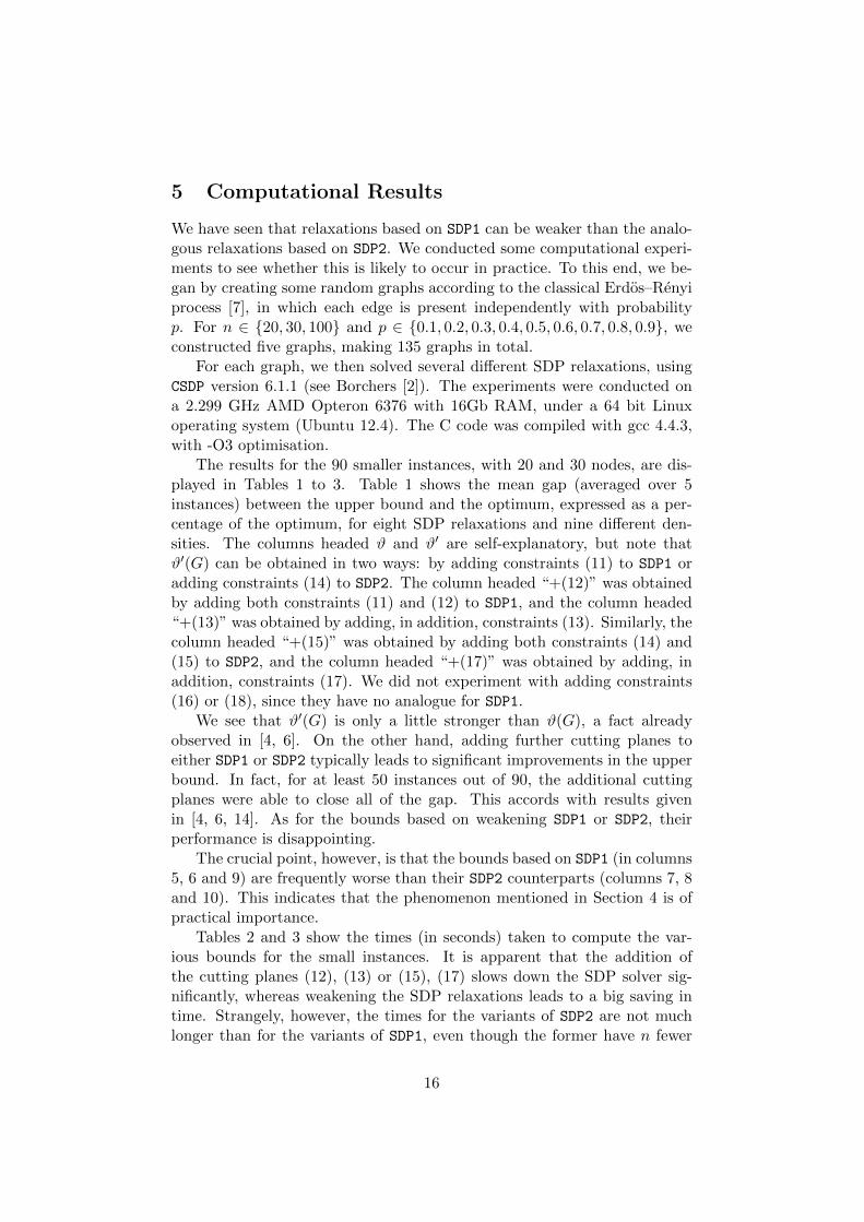
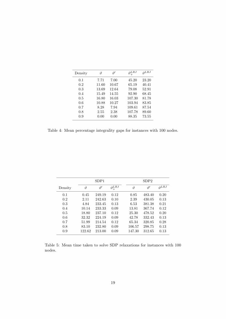
For the instances with 100 nodes, the SDP solver was unable to computesome of the stronger bounds in a reasonable amount of time. The resultswith the remaining bounds are shown in Tables 4 and 5. We see that, again,ϑ′(G) is only a little stronger than ϑ(G), ϑLRJ(G) is much weaker, andϑLRJ+ (G) is much weaker still. As for running times, the effect of adding oraggregating constraints is even more marked. Moreover, we now see that thebounds based on SDP2 now take about 50% longer to compute than thosebased on SDP1.

6 Concluding Remarks

It has been known since the 1980s [13] that the Lovasz theta function can becomputed by solving either of two equivalent SDPs, which we have labelledSDP1 and SDP2. We have shown, however, that the equivalence betweenSDP1 and SDP2 breaks down when they are either strengthened (via cuttingplanes) or weakened (via constraint aggregation).

Our results have implications for the development of exact algorithmsfor the maximum stable set problem. In a branch-and-bound algorithm, atrade-off must be made between the quality of the upper bound and the time

17

n Density ϑ ϑ′ +(12) +(13) ϑLRJ+

0.1 0.00 0.03 0.90 8.43 0.000.2 0.01 0.03 2.66 9.97 0.000.3 0.01 0.03 6.26 13.00 0.000.4 0.01 0.03 12.79 18.03 0.00

20 0.5 0.01 0.02 18.37 22.20 0.000.6 0.01 0.02 34.28 35.41 0.000.7 0.02 0.02 61.24 59.58 0.000.8 0.03 0.03 84.54 78.52 0.000.9 0.04 0.02 95.45 90.67 0.00

0.1 0.01 0.42 18.02 345.17 0.010.2 0.02 0.24 58.52 316.61 0.010.3 0.03 0.44 204.57 484.02 0.010.4 0.04 0.23 405.88 665.35 0.01

30 0.5 0.08 0.42 843.04 1053.02 0.010.6 0.10 0.23 1505.87 1673.03 0.010.7 0.18 0.25 2618.84 2610.24 0.010.8 0.16 0.19 3222.37 3166.29 0.010.9 0.23 0.21 4124.27 3857.24 0.01

Table 2: Mean time taken to solve relaxations based on SDP1.

n Density ϑ ϑ′ +(15) +(17) ϑLRJ

0.1 0.01 0.04 0.88 8.89 0.010.2 0.01 0.04 3.55 12.18 0.010.3 0.01 0.05 7.73 15.23 0.000.4 0.02 0.05 14.73 20.41 0.01

20 0.5 0.02 0.04 20.33 24.04 0.010.6 0.02 0.04 39.82 41.08 0.000.7 0.03 0.04 64.19 61.60 0.010.8 0.04 0.04 82.08 77.82 0.010.9 0.05 0.03 106.64 101.67 0.01

0.1 0.02 0.63 18.38 367.98 0.010.2 0.02 0.35 69.34 415.20 0.010.3 0.04 0.63 214.68 572.30 0.010.4 0.06 0.33 433.66 736.79 0.01

30 0.5 0.11 0.56 790.25 1041.33 0.010.6 0.14 0.37 1537.81 1711.69 0.010.7 0.20 0.35 2589.68 2673.10 0.020.8 0.22 0.30 2948.88 2989.95 0.010.9 0.31 0.26 3854.47 3850.89 0.01

Table 3: Mean time taken to solve relaxations based on SDP2.

18

Density ϑ ϑ′ ϑLRJ+ ϑLRJ

0.1 7.71 7.00 45.20 23.200.2 11.60 10.67 65.19 40.410.3 13.69 12.64 79.08 52.910.4 15.49 14.55 92.90 68.450.5 16.80 16.03 107.30 81.780.6 10.88 10.27 103.94 83.850.7 8.28 7.94 109.61 87.540.8 2.55 2.38 107.78 89.600.9 0.00 0.00 88.35 73.55

Table 4: Mean percentage integrality gaps for instances with 100 nodes.

SDP1 SDP2

Density ϑ ϑ′ ϑLRJ+ ϑ ϑ′ ϑLRJ

0.1 0.45 249.19 0.12 0.85 483.40 0.200.2 2.11 242.63 0.10 2.39 430.05 0.130.3 4.84 233.45 0.13 6.53 381.38 0.210.4 10.14 233.33 0.09 13.81 367.74 0.120.5 18.80 237.10 0.12 25.30 478.52 0.200.6 32.32 224.19 0.09 42.78 332.43 0.130.7 51.99 214.54 0.12 65.34 320.85 0.280.8 83.10 232.80 0.09 106.57 298.75 0.130.9 122.62 213.00 0.09 147.30 312.65 0.13

Table 5: Mean time taken to solve SDP relaxations for instances with 100nodes.

19

taken to compute it. If one wishes to use the theta function itself as theupper bound, then SDP1 is to be preferred to SDP2. If, however, one wishes touse a strengthened or weakened variant of the theta number, then the choicebetween SDP1 and SDP2 is no longer obvious, and further experimentationwill be needed.

References

[1] E. Balas, S. Ceria, G. Cornuejols & G. Pataki (1996) Polyhedral meth-ods for the maximum clique problem. In D.S. Johnson & M.A. Trick(eds.) Cliques, Coloring and Satisfiability: The 2nd DIMACS Imple-mentation Challenge. Providence, RI: American Mathematical Society.

[2] B. Borchers (1999) CSDP, a C library for semidefinite programming.Optim. Meth. & Software, 11, 613–623.

[3] R. Borndorfer (1998) Aspects of Set Packing, Partitioning and Cover-ing. Doctoral Thesis, Technical University of Berlin.

[4] S. Burer & D. Vandenbussche (2006) Solving lift-and-project relax-ations of binary integer programs. SIAM J. Opt., 16, 726–750.

[5] M.M. Deza & M. Laurent (1997) Geometry of Cuts and Metrics. Berlin:Springer-Verlag.

[6] I. Dukanovic & F. Rendl (2007) Semidefinite programming relaxationsfor graph coloring and maximal clique problems. Math. Program., 109,345–365.

[7] P. Erdos & A. Renyi (1959) On random graphs. Publicationes Mathe-maticae, 6, 290–297.

[8] U. Feige & J. Kilian (1998) Zero-knowledge and the chromatic number.J. Comput. Syst. Sci., 57, 187–199.

[9] M. Giandomenico & A.N. Letchford (2006) Exploring the relationshipbetween max-cut and stable set relaxations. Math. Program., 106, 159-175.

[10] M. Giandomenico, A.N. Letchford, F. Rossi & S. Smriglio (2009) Anapplication of the Lovasz-Schrijver M(K,K) operator to the stable setproblem. Math. Program., 120, 381–401.

[11] M. Giandomenico, F. Rossi & S. Smriglio (2013) Strong lift-and-projectcutting planes for the stable set problem. Math. Program. , 141, 165–192.

20

[12] M. Grotschel, L. Lovasz & A.J. Schrijver (1981) The ellipsoid methodand its consequences in combinatorial optimization. Combinatorica, 1,169–197.

[13] M. Grotschel, L. Lovasz & A.J. Schrijver (1988) Geometric Algorithmsand Combinatorial Optimization. New York: Wiley.

[14] G. Gruber & F. Rendl (2003) Computational experience with stable setrelaxations. SIAM J. Opt., 13, 1014–1028.

[15] J. Hastad (1999) Clique is hard to approximate within n1−ε. Acta Math.,182, 105–142.

[16] M. Laurent (2001) A comparison of the Sherali-Adams, Lovasz-Schrijver and Lasserre relaxations for 0-1 programming. Math. Oper.Res., 28, 470–496.

[17] F. Lieder, F. Rad & F. Jarre (2015) Unifying semidefinite and set-copositive relaxations of binary problems and randomization tech-niques. Comput. Optim. Appl., 61, 669–688.

[18] L. Lovasz (1979) On the Shannon capacity of a graph. IEEE Trans.Inform. Th., 25, 1–7.

[19] L. Lovasz & A.J. Schrijver (1991) Cones of matrices and set-functionsand 0-1 optimization. SIAM J. Opt., 1, 166–190.

[20] G.L. Nemhauser & G. Sigismondi (1992) A strong cutting-plane / branch-and-bound algorithm for node packing. J. Oper. Res.Soc., 43, 443–457.

[21] M.W. Padberg (1973) On the facial structure of set packing polyhedra.Math. Program., 5, 199–215.

[22] M.W. Padberg (1989) The Boolean quadric polytope: some character-istics, facets and relatives. Math. Program., 45, 139–172.

[23] S. Rebennack, M. Oswald, D.O. Theis, H. Seitz, G. Reinelt &P.M. Pardalos (2011) A branch and cut solver for the maximum stableset problem. J. Combin. Optim., 21, 434–457.

[24] F. Rossi & S. Smriglio (2001) A branch-and-cut algorithm for the max-imum cardinality stable set problem. Oper. Res. Lett., 28, 63–74.

[25] A.J. Schrijver (1979) A comparison of the Delsarte and Lovasz bounds.IEEE Trans. Inf. Th., IT-25, 425–429.

[26] E.A. Yildirim & X. Fan–Orzechowski (2006) On extracting maximumstable sets in perfect graphs using Lovaszs theta function. Comput.Optim. Appl., 33, 229–247.

21