ON THE CIRCLE CRITERION FOR BOUNDARY CONTROL SYSTEMS...

ON THE CIRCLE CRITERION FOR BOUNDARY CONTROL SYSTEMSIN FACTOR FORM: LYAPUNOV STABILITY AND LUR’E EQUATIONS

PIOTR GRABOWSKI AND FRANK M. CALLIER

Abstract. A Lur’e feedback control system consisting of a nonlinear static sector typecontroller and a linear, infinite–dimensional system of boundary control in factor form isconsidered. A criterion of absolute strong asymptotic stability of the null equilibrium isobtained using a quadratic form Lyapunov functional. The construction of such functionalis reduced to solving a Lur’e system of equations. For the solvability of the latter themain result is a sufficient condition using the strict circle inequality based on results byJ.C. Oostveen and R.F. Curtain [27]. All results are illustrated in detail by electricaltransmission line examples: 1) of the distortionless loaded RLCG–type and 2) of theunloaded RC–type.

Contents

1. Introduction 12. Preliminary data 23. Asymptotic stability of the Lur’e feedback system 74. Sufficient criterion for solvability of the Lur’e system of equations 114.1. Spectral factorization 114.2. State–feedback realization problem 124.3. Sufficient criterion using a strict circle inequality 135. Example 1: Distortionless loaded RLCG–transmission line 175.1. The case of nonpositive b 195.2. The case of positive b 206. Example 2: Unloaded RC–transmission line 227. Discussion and conclusions 25References 26

1. Introduction

This paper uses some results of abstract linear systems in factor form, obtained by theauthors in earlier papers [16], [17] and shortly recalled in Section 2; these systems are relatedbut not identical to Salamon–Weiss abstract linear systems e.g. [36], see [16, Section 4.5],[17, Section 7]. The results of Section 2 combined with the input–output approach usingpassivity concepts lead in [18] to a circle criterion for the nonlinear Lur’e type feedbacksystem described by Figure 3.1 below, consisting of a nonlinear static sector type controllerfollowed by a linear infinite–dimensional system of boundary control in factor form in the

Date: March 22, 2002.1991 Mathematics Subject Classification. Primary: 93B, 47D. Secondary: 35A, 34G.Key words and phrases. infinite–dimensional control systems, semigroups, Lyapunov functionals, circle

criterion.

2 PIOTR GRABOWSKI AND FRANK M. CALLIER

loop. The present paper shows that Lyapunov state space theory together with the abstractresults of Section 2 gives similar stability conditions.

An absolute stability criterion is derived in Section 3. It is obtained by using a quadraticform Lyapunov functional. An intricate procedure of evaluating the derivative of thequadratic form along the system trajectories is studied and successfully applied to geta novel so–called Lur’e system. The abstract results of Section 2 enable us to proveglobal strong asymptotic stability of the null equilibrium in Theorem 3.1. An importantconsequence is that the stability question depends on the solvability of the Lur’e systemof equations (3.2) (or equivalently (3.3)).

This reduction is standard in finite–dimensional state space system theory and leadsto a variety of solvability results commonly known as the Kalman–Popov lemma and theYacubovic frequency–domain theorem. The main difficulty in getting a generalization ofthis lemma in the infinite–dimensional case is due to the fact that the open–loop linearsystem control and/or observation involve unbounded linear operators, which lead to somedifficult mathematical questions. However it turns out that the proof of the Riccati results[27, Theorem 19 and Corollary 20] of Oostveen and Curtain is useful in our context. Itsadaptation (with in particular Lemma 4.3) is essential in Section 4 on the solvability ofthe Lur’e system (3.2). It proceeds, modulo adaptation involving the transfer functionmapping g(s) 7−→ g(s−1) − g(0), as in the spectral factorization method for solving theRiccati equation of Callier and Winkin [7]. One starts by giving appropriate spectralfactorization results. Next one describes a state–feedback observation operator realizationproblem induced by a spectral factor, see (4.7). Finally the solvability of the Lur’e systemis obtained in Theorem 4.1. Many other Lur’e system results are available such as [26,Theorem 4, p. 570], [22, Theorem 3, p. 902], [24], [2, Theorem 2.1, p. 179], [28, Theorem3, p. 740], [4, Theorem 3.1], [29, Theorem 2] and [30, Theorem 3, p. 482]. However theydo not fit our context.

Sections 5 and 6 present an exhaustive illustration of the results for the examples of

* a loaded distortionless electric RLCG–transmission line for which we prove theglobal strong asymptotic stability,

* an unloaded electric RC–transmission line for which we prove the global strongasymptotic stability too, despite the fact that here the factor control vector d isnot admissible and only a weaker stability result follows from the proof of Theorem3.1.

Related, although different absolute stability results have been proved in [3], [4] and [23].A discussion and some prospects for further investigations are presented in the concludingSection 7.

2. Preliminary data

We start by recalling the notion of admissibility of output operators. To do this, ina Hilbert space H with a scalar product 〈·, ·〉H, consider the homogeneous system withobservation

x(t) = Ax(t)

x(0) = x0

y(t) = Cx(t)

, t ≥ 0 .

We assume that A : (D(A) ⊂ H) −→ H generates a linear C0–semigroup {S(t)}t≥0 on Hand C ∈ L(DA,Y) is an observation (output) operator, where DA stands for the space

CIRCLE CRITERION: LYAPUNOV APPROACH 3

D(A) equipped with the graph norm and Y is an another Hilbert space with a scalarproduct 〈·, ·〉Y.

Definition 2.1. The observation operator C is called (infinite–time) admissible if theobservability operator P : H −→ L2(0,∞; Y), (Px)(t) := CS(t)x is defined and boundedon D(A).

If the observation operator C is admissible then: P is densely defined, closable and forany x ∈ D(A) the function [0,∞) 3 t 7−→ (Px)(t) = CS(t)x ∈ Y is continuous. By thestandard operator theory P ∗ ∈ L(L2(0,∞; Y),H) and P = P ∗∗ ∈ L(H,L2(0,∞; Y)).

Standard arguments involving continuity, the fact that D(A) is dense in H, and theclosed graph theorem lead to the following result also mentioned in [36] and [27].

Lemma 2.1. An operator C ∈ L(H,Y) is admissible iff CS(·)x ∈ L2(0,∞; Y) for anyx ∈ H.

In addition to Lemma 2.1 observe that if C ∈ L(H,Y) is admissible then the adjoint ofP is given by

P ∗y =

∫ ∞0

S∗(t)C∗y(t)dt, y ∈ L2(0,∞; Y) .

Consequently the admissibility for bounded control operators can be introduced by usingadjoint operators. An operator B ∈ L(U,H), where U stands for a Hilbert space withscalar product 〈·, ·〉U, is said to be an (infinite–time) admissible control operator if itsadjoint B∗ ∈ L(H,U) is an admissible observation operator with respect to the adjointsemigroup, i.e. if the observability map x 7−→ B∗S∗(·)x is everywhere defined on H, nowwith output space U. The latter fact is necessary and sufficient for Q ∈ L(L2(0,∞; U),H)where Q is the reachability operator given by

Qu =

∫ ∞0

S(t)Bu(t)dt .

In this paper we shall consider mainly SISO systems of boundary control in factor form[16],

(2.1)

{x(t) = A[x(t) + u(t)d]

y = c#x

}.

assuming, if something else is not explicitly said, that A : (D(A) ⊂ H) −→ H generates alinear exponentially stable (EXS), C0–semigroup {S(t)}t≥0 on H, d ∈ H is a factor controlvector, u ∈ L2(0,∞) is a scalar control function, y is a scalar output defined by an A–bounded linear observation functional c# (bounded on DA). The restriction of c# to D(A)is representable as c#

∣∣D(A)

= h∗A for some h ∈ H.

Define two operators:

V ∈ L(H,L2(0,∞)), (V x)(t) := h∗S(t)x

W ∈ L(L2(0,∞),H), Wu :=

∫ ∞0

S(t)du(t)dt .

Recall that L and R = L∗,

Lf = f ′, D(L) = W1,2(0,∞) ,

Rf = −f ′, D(R) = {f ∈W1,2(0,∞) : f(0) = 0}


are the generators of the semigroups of left– and right–shifts on L2(0,∞), respectively.With these notation and assumptions Definition 2.1 gets the following equivalent form.

Definition 2.2. The observation functional c# is called admissible if the observabilityoperator

P = V A, D(P ) = D(A)

has a bounded continuous extension on H denoted by P .

Definition 2.3. The factor control vector d ∈ H is called admissible if

Range(W ) ⊂ D(A) .

Remark 2.1. By Definition 2.3, W ∈ L(L2(0,∞),H) because the semigroup {S(t)}t≥0 isEXS. Moreover, the reachability operator Q satisfies Q := AW ∈ L(L2(0,∞),H).

In the sequel Π+ := {s ∈ C : Re s > 0} denotes the open right–half complex plane,H∞(Π+) is the Banach space of analytic functions f on Π+, equipped with the norm‖f‖H∞(Π+) = sup

s∈Π+

|f(s)| and H2(Π+) is the Hardy space of functions f analytic on Π+ such

that supσ>0

∫ ∞−∞|f(σ + jω)|2 dω < ∞, where f(jω) := lim

σ→0+f(σ + jω) exists for almost all

ω ∈ R. The space H2(Π+) is unitarily isomorphic with L2(0,∞) through the normalizedLaplace transform. To be more precise,

〈f, g〉L2(0,∞) =1

2π

∫ ∞−∞

f(jω)g(jω)dω

where f , g are the Laplace transform of f and g, respectively.Moreover [21, p. 134] we shall frequently use the unitary operator U ∈ L(H2(Π+)) given

by

(2.2) (Uϕ)(s) := (1/s)ϕ(1/s) ,

which for the jω–axis H2(Π+)–norm corresponds to the change of variable ω 7−→ −ω−1.Finally we shall encounter Wiener and Callier–Desoer convolution algebras. Recall [5,

pp. 652 - 653], [6, pp. 81 - 84], [8, pp. 337 - 338] that a scalar–valued Laplace transformabledistribution f with support on [0,∞) is in the Wiener class A(σ) for some σ ∈ R if

f(t) = fa(t) + fsa(t) for t ≥ 0 with e−σ(·)fa(·) ∈ L1(0,∞) and fsa(t) =∞∑i=0

fiδ0(t − ti),

where δ0 denotes the Dirac delta distribution and t0 = 0 and ti > 0 for i > 0 are such

that∞∑i=0

e−σti |fi| < ∞. Such distribution is in the Callier–Desoer class A−(0) if it is in

A(σ) for some σ < 0. A(σ) and A−(0) denote the classes of Laplace transforms of suchdistributions. A(σ) is a convolution Banach algebra with norm

‖f‖A(σ) :=∥∥e−σ(·)fa(·)

∥∥L1(0,∞)

+∞∑i=0

e−σti |fi| .

For more information see [6] or [8].

Definition 2.4. The operator H ∈ L(L2(0,∞)) is called causal or nonanticipative if

(HuT )T = (Hu)T ∀u ∈ L2(0,∞)


where uT denotes the truncation of u at time T > 0, uT (t) =

{u(t) if t < T0 otherwise

}.

Lemma 2.2. If c# is admissible then P , the closure of P has the form

Range(V ) ⊂ D(L), P = LV

In particular for all x0 ∈ H, (Px0)(t) =d

dt[h∗S(t)x0] ∈ L2(0,∞) with Laplace transform(

P x0

)(s) = c#(sI − A)−1x0 ∈ H2(Π+). Moreover if d is admissible then the reachability

operator Q = AW belongs to L(L2(0,∞),H).

Lemma 2.3. If the compatibility condition

(2.3) d ∈ D(c#)

holds then the function

(2.4) g(s) := sc#(sI − A)−1d− c#d = sh∗A(sI − A)−1d− c#d

is well–defined and analytic on the complex right half–plane Π+.If in addition to (2.3), c# is admissible then:

(i) g(s) = s(P d)(s)− c#d with P d ∈ H∞(Π+) ∩ H2(Π+).

(ii) The convolution operator K with kernel Pd, i.e., Ku := Pd?u belongs to L(L2(0,∞))and it maps the domain of R into itself.

Lemma 2.3 leads to the following result [17, Theorem 4.1, Corollary 4.1, Theorem 4.2].

Lemma 2.4. If (2.3) holds, c# is admissible and

(2.5) g ∈ H∞(Π+)

then the input–output operator F ,

F = −KR− c#dI, D(F ) = D(R)

is bounded and its closure F is causal and given by

Range(K) ⊂ D(R), F = −RK − c#dI .

Moreover g is then the transfer function of the system (2.1), and F is a convolution operatorin the sense of distributions given by

Fu = g ? u, u ∈ L2(0,∞) ,

with impulse response g given by

g := D(Pd)− c#dδ0 ,

with Laplace transform g (here D denotes the distributional derivative, and δ0 stands forthe Dirac distribution at zero).

If in addition

c# ⊂ c#L ,

where

c#Lx0 = lim

h→0+

1

hc#

∫ h

0

S(σ)x0dσ, D(c#L ) =

{x0 ∈ H : ∃ lim

h→0+

1

hc#

∫ h

0

S(σ)x0dσ

}


is the Lebesgue extension of c#, then c#d =(Pd)

(0+) i.e. the Lebesgue value given by(Pd)

(0+) := limt→0+

1

t

∫ t

0

(Pd)

(τ)dτ = lims→∞,s∈R

s(Pd)(s),

andlim

s→∞,s∈Rg(s) = 0 .

The following auxiliary result [17, Fact 3.2, p. 8] shall be needed.

Lemma 2.5. Let c# be admissible. Let ω < 0 be the growth constant of the EXSC0–semigroup generated by A on H. Then for any σ ∈ (ω, 0](

t 7−→ e−σt(Px0

)(t))∈ L1(0,∞) ∩ L2(0,∞) ∀x0 ∈ H .

As a consequence with d ∈ H,(P d)(s) ∈ A(σ) for any σ ∈ (ω, 0], and hence for such σ, is

analytic and bounded in Re s > σ and thus also in a full neighborhood of s = 0.

In the sequel σ(·), σP (·), σC(·) will respectively denote the spectrum, the point (i.e.discrete) spectrum and the continuous spectrum of an operator. We shall need

Lemma 2.6. Let A : (D(A) ⊂ H) −→ H be the generator an EXS C0–semigroup {S(t)}t≥0

on H. Then the semigroup {etA−1}t≥0, generated by A−1 ∈ L(H), is strongly asymptotically

stable (AS), i.e. for every x0 ∈ H, limt→∞

etA−1

x0 = 0, if and only if {etA−1}t≥0 is uniformly

bounded.

Proof. If the semigroup {S(t)}t≥0 is EXS, then σP (A−1) ∩ jR = ∅, σP((A∗)−1

)∩ jR = ∅

and 0 ∈ σC(A−1) is the only possible point of the spectrum ofA−1 on jR. This together with

the assumption that {etA−1}t≥0 is uniformly bounded gives that the semigroup {etA−1}t≥0

is AS by [1, Stability Theorem, p. 837], see also [25].

Conversely, if {etA−1}t≥0 is AS, then for all x ∈ H, supt≥0 ‖etA−1x‖H <∞, such that by

the uniform boundedness principle supt≥0 ‖etA−1‖L(H) <∞, whence {etA−1}t≥0 is uniformly

bounded. �

Corollary 2.1. Let A : (D(A) ⊂ H) −→ H be the generator an EXS C0–semigroup

{S(t)}t≥0 on H. Then the semigroup {etA−1}t≥0 is AS if the operator inequality

(2.6) 〈Ax,Xx〉H + 〈Xx,Ax〉H ≤ 0 ∀x ∈ D(A) .

has a bounded self–adjoint solution X = X∗ ∈ L(H) which is coercive.

Remark 2.2. This means that A is similar to a dissipative operator, [31, p.13] (to see thisput X = W ∗W , where W ∈ L(H) is a Banach isomorphism).

Proof. Put in (2.6) X = W ∗W , where W ∈ L(H) is a Banach isomorphism, and setz := WAx. The latter defines a bijection of D(A) onto H such that z is an arbitrary pointof H. Hence (2.6) reduces to

Re〈(WA−1W−1)z, z〉H ≤ 0 ∀z ∈ H .

This means that the similar generator WA−1W−1 as well as its adjoint are dissipative.Hence by [31, Corollary 4.4, p.15], {et(WA−1W−1) = WetA

−1W−1}t≥0 is a contraction semi-

group, i.e. ∥∥et(WA−1W−1)∥∥L(H)≤ 1 ∀t ≥ 0 .


Therefore ∥∥etA−1∥∥L(H)≤∥∥W−1

∥∥L(H)‖W‖L(H) <∞ ∀t ≥ 0 ,

and the conclusion follows by Lemma 2.6. �

Corollary 2.2. Let A : (D(A) ⊂ H) −→ H be the generator an EXS C0–semigroup

{S(t)}t≥0 on H. Let σ(A) = σP (A) and let H have a Riesz basis of eigenvectors of A. Then

the semigroup {etA−1}t≥0 is AS.

Proof. Here A is similar to the diagonal operator Λ of eigenvalues of A, which is dissipativeas {S(t)}t≥0 is EXS. Hence the conclusion follows by Corollary 2.1 and Remark 2.2. �

3. Asymptotic stability of the Lur’e feedback system

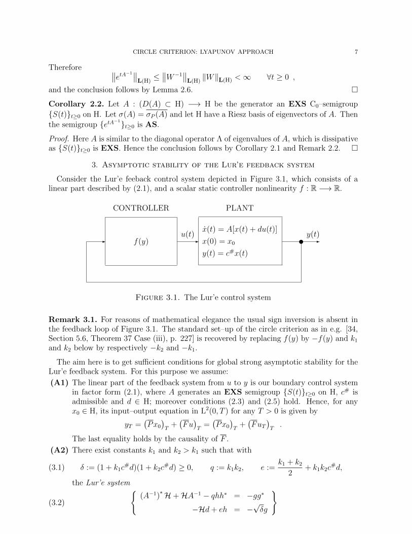
Consider the Lur’e feeback control system depicted in Figure 3.1, which consists of alinear part described by (2.1), and a scalar static controller nonlinearity f : R −→ R.

u y(t)

CONTROLLER

u(t)

PLANT

f(y)

x(t) = A[x(t) + du(t)]

x(0) = x0

y(t) = c#x(t)

- --

Figure 3.1. The Lur’e control system

Remark 3.1. For reasons of mathematical elegance the usual sign inversion is absent inthe feedback loop of Figure 3.1. The standard set–up of the circle criterion as in e.g. [34,Section 5.6, Theorem 37 Case (iii), p. 227] is recovered by replacing f(y) by −f(y) and k1

and k2 below by respectively −k2 and −k1.

The aim here is to get sufficient conditions for global strong asymptotic stability for theLur’e feedback system. For this purpose we assume:

(A1) The linear part of the feedback system from u to y is our boundary control systemin factor form (2.1), where A generates an EXS semigroup {S(t)}t≥0 on H, c# isadmissible and d ∈ H; moreover conditions (2.3) and (2.5) hold. Hence, for anyx0 ∈ H, its input–output equation in L2(0, T ) for any T > 0 is given by

yT =(Px0

)T

+(Fu)T

=(Px0

)T

+(FuT

)T.

The last equality holds by the causality of F .

(A2) There exist constants k1 and k2 > k1 such that with

(3.1) δ := (1 + k1c#d)(1 + k2c

#d) ≥ 0, q := k1k2, e :=k1 + k2

2+ k1k2c

#d,

the Lur’e system

(3.2)

{(A−1)

∗H +HA−1 − qhh∗ = −gg∗

−Hd+ eh = −√δg

}


has a solution (H, g), g ∈ H, H ∈ L(H), H = H∗ ≥ 0, or so does the equivalentsystem

(3.3)

{〈Ax,Hx〉H + 〈x,HAx〉H = q (h∗Ax)2 − (g∗Ax)2 ∀x ∈ D(A)

−Hd+ eh = −√δg

}.

(A3) The factor control vector d ∈ H is admissible.

Next for the controller two sets describe restrictions to be imposed on the static nonlinearityf : R −→ R, namely

• For sufficiently small ε > 0, we define the sector:

Sε :=

{f ∈ C(R) : −∞ < k1 <

1

2

[k1 + k2 −

√(k2 − k1)2 − 4ε

]≤ f(y)

y≤

≤ 1

2

[k1 + k2 +

√(k2 − k1)2 − 4ε

]< k2 <∞ ∀y ∈ R \ {0} , f(0) = 0

}.

In the sequel we shall also use S0 := limε→0+

Sε.• We denote by M the class of those functions f ∈ S0 ∩ C(R) which are sufficiently

smooth such that for the given Lur’e feedback system, for any x0 ∈ H, the truncatedoutput yT belongs to L2(0, T ) for any T > 0, i.e it solves the closed–loop fixed pointoutput equation

yT =(Px0

)T

+(Ff(yT )

)T.

Lemma 3.1. Let assumption (A1) hold. Let f belong to M. Then:

(i) For any T > 0 the truncated output yT and input uT (u = f(y)) is in L2(0, T ).(ii) If moreover (A3) holds, then the closed–loop state differential equation

(3.4)

{x = A[x+ df(y)]

x(0) = x0 ∈ H

}has for any T > 0 the weak solution x(·) ∈ C(0, T ; H) given by

(3.5) x(t) = S(t)x0 + A

∫ t

0

S(t− τ)df(y(τ)

)dτ, t ≥ 0 ,

which satisfies pointwise in H almost everywhere

(3.6)

d

dt

[A−1x

]= A−1x = x+ df(y)

x(0) = x0 ∈ H

.

Proof. Ad (i). As f ∈M one gets that for any T > 0 the truncation yT is in L2(0, T ) andmoreover

‖u‖L2(0,T ) ≤ max {|k1|, |k2|} ‖y‖L2(0,T )

Ad (ii). By (i) and (A3) formula (3.5) of the weak solution x(·) ∈ C(0, T ; H) of (3.4)holds by the analysis in [16, Section 4.2]. Next by Fubini’s theorem with u = f(y)∫ t

0

[x(τ) + du(τ)] dτ = A−1[x(t)− x0], t ≥ 0 ,

such that, by Lebesgue’s differentiation theorem for vector–valued functions, (3.6) holdspointwise in H almost everywhere. �


Remark 3.2. For w ∈ D(A∗) one has

d

dt〈w, x〉H =

d

dt〈A∗w,A−1x〉H = 〈A∗w,A−1x〉H = 〈A∗w, x+ df(y)〉H

whence any pointwise a.e. solution of (3.6) is a weak solution of (3.4). The point is thatthe converse holds.

Theorem 3.1. Let assumptions (A1)÷(A3) hold. Let f belong to Sε ∩M. Then theorigin of the space H is globally strongly asymptotically stable (GSAS).

Proof. The objective is to get the quadratic form V (x) = x∗Hx as a Lyapunov functionalfor the system (3.6). With f ∈ M and u = f(y) its derivative along the solutions of (3.6)reads as

V = x∗Hx+ x∗Hx = x∗H(A−1x− du) + (A−1x− du)∗Hx =

=

[x

u

]∗ [ HA−1 + (A−1)∗H −Hd

−d∗H 0

][x

u

].

Moreover with y = c#x = c#A−1x− c#df(y) = h∗x− c#du

[k2y − u][u− k1y] = [k2h∗x− (k2c

#d+ 1)u][(k1c#d+ 1)u− k1h

∗x] ,

which by adding and subtracting gives

V = −(k2y − u)(u− k1y) +

[x

u

]∗ [ HA−1 + (A−1)∗H− qhh∗ −Hd+ eh

−d∗H + eh∗ −δ

][x

u

].

Hence (A2) gives

V = −[g∗x+

√δu]2

− (k2y − u)(u− k1y) ≤ 0 .

Thus for f ∈M, V is a Lyapunov functional for the system (3.6). Now, due to f ∈ Sε, wehave

(3.7) V = −[g∗x+

√δu]2

− (k2y − u)(u− k1y) ≤ −εy2 .

This is because{1

2

[k1+k2−

√(k2 − k1)2 − 4ε

]y−u

}{u− 1

2

[k1+k2+

√(k2 − k1)2 − 4ε

]y}

= (k2y − u)(u− k1y)− εy2

Integrating both sides of (3.7) from 0 to t and using H ≥ 0 we obtain,

−V (x0) ≤ V [x(t, x0)]− V (x0) ≤ −ε∫ t

0

y2(τ)dτ

whence

‖H‖L(H) ‖x0‖2H ≥ V (x0) ≥ ε

∫ t

0

y2(τ)dτ .

This yields

‖y‖L2(0,∞) ≤√

1

ε‖H‖L(H) ‖x0‖H .

Since f ∈ S0∫ ∞0

u2(t)dt =

∫ ∞0

f 2[y(t)]dt =

∫ ∞0

y2(t)f 2[y(t)]

y2(t)dt ≤ max

{k2

2, k21

}‖y‖2

L2(0,∞) ,


whence

(3.8) ‖u‖L2(0,∞) ≤ max {|k2|, |k1|}√

1

ε‖H‖L(H) ‖x0‖H .

Hence there holds that y, u ∈ L2(0,∞).Since, by (A3), d ∈ H is an admissible factor control vector, then

(3.9) x(t) = S(t)x0 +QRtu t ≥ 0

where Q ∈ L(L2(0,∞),H) is the reachability map of Remark 2.1 and Rt ∈ L(L2(0,∞))denotes the reflection operator at t > 0,

(Rtu)(τ) :=

{u(t− τ), τ ∈ [0, t)

0, τ ≥ t

}, ‖Rt‖L(L2(0,∞)) ≤ 1 .

There holds that 0 ≤ t 7−→ x(t) ∈ H is strongly continuous. Using (3.8) and recalling thatthe exponential stability of the semigroup {S(t)}t≥0 implies by the principle of uniformboundedness its stability (i.e the uniform boundedness for t ≥ 0), we conclude that thereexists a constant γ > 0, such that

(3.10) ‖x(t)‖H ≤ γ ‖x0‖H ∀x0 ∈ H, ∀t ≥ 0 .

The stability of the null equilibrium easily follows from (3.10).Considering state–attraction to zero, there holds that ‖S(t)x0‖H tends to zero as t→∞

for any x0 ∈ H. Hence we may without loss of generality consider x(t) = QRtu. For anyfixed u ∈ L2(0,∞) define for t1 > 0

ut1(t) :=

{0, t ∈ [0, t1)

u(t), t ≥ t1

}.

One gets then that for t ≥ t1

x(t) = QRtu = S(t− t1)QRt1u+QRtut1 ,

where {S(t)}t≥0 is EXS,

‖QRtut1‖H ≤ ‖Q‖L(L2(0,∞),H) ‖Rt‖L(L2(0,∞)) ‖ut1‖L2(0,∞) ≤ ‖Q‖L(L2(0,∞),H) ‖ut1‖L2(0,∞) ,

and ‖ut1‖L2(0,∞) can be made arbitrarily small for t1 sufficiently large. Therefore similarly

as in the proof of [27, Lemma 12] one gets that limt→∞‖x(t)‖H = 0. �

The final part of the proof of Theorem 3.1 relies on the observation that the admissibilityof d implies two facts:

. QR(·) ∈ L(L2(0,∞),L2(0,∞; H)),

. limt→∞‖QRtu‖H = 0 ∀u ∈ L2(0,∞) (or even Range(QR(·)) ⊂ BUC0[0,∞; H) [18]).

Here we tacitly assumed the worst case where the controller can generate any control signalu ∈ L2(0,∞). In fact the control signal is being produced from the feedback loop as it isexplained by the operator–theoretic diagram depicted in Figure 3.2.

Predicting some facts which will be rigorously stated in Section 6 we announce here thatin an abstract parabolic case where A generates an EXS analytic semigroup all systemoperators: S, QR(·), P and F feature some balanced smoothing properties. Thanks to

this even if d is not admissible one can still have QR(·) ∈ L(L2(0,∞),L2(0,∞; H)) andlimt→∞‖QRtu‖H = 0 now only for controls truly generated by the feedback. These last two


P -� ��- f ∈ Sε QRt-� �� -

F

?-s

S(t)

-?sx0 +

+ ++y u x(t)

CONTROLLER

Figure 3.2. The operator–theoretic diagram of the Lur’e control system

facts turn out to be sufficient for proving that the origin is GSAS under some assumptionsimposed on d which are essentially weaker than (A3).

4. Sufficient criterion for solvability of the Lur’e system of equations

In this section we shall get sufficient conditions for checking (A2), i.e. for the solvabilityof the Lur’e system of equations (3.2) or equivalently (3.3) with respect to the pair (H, g).Our inspiration stems from the Oostveen and Curtain Riccati results in [27], modulo adap-tation to our context, where d is not supposed to be admissible i.e. (A3) does not holdas an intellectual challenge motivated by the ”parabolic regularity” mentioned above andexamined in detail in Section 6 where d is not admissible.

The method for getting our main result Theorem 4.1 is as in the spectral factorizationmethod for solving the Riccati equation of Callier and Winkin [7], modulo the transferfunction mapping g(s) 7−→ g(s−1) − g(0). Spectral factorization is handled first. Someother preliminary results follow next, and finally we get our result.

4.1. Spectral factorization. The following result is important in our context.

Lemma 4.1. Let ω 7−→ π(jω) be a real–valued, nonnegative function on the jω–axis suchthat π belongs to L∞(R) and π(jω) = π(−jω). Let in addition π be coercive, i.e. thereexists an ε > 0 such that π(jω) ≥ ε for all ω ∈ R. Then:

(i) There exists a function φ ∈ H∞(Π+) such that

(4.1) π(jω) = φ(jω)φ(−jω) = |φ(jω)|2 ,

and 1/φ is as well in H∞(Π+). Moreover φ(s) can be chosen to be real, i.e. it satisfies

φ(s) = φ(s), meaning that a Taylor expansion in the open right–half plane has realcoefficients or that φ(s) takes real values for real arguments; furthermore such φ(s) isunique modulo a ±1 factor.

(ii) If moreover π(jω) has an analytic extension in a domain containing a full neighborhoodof s = 0 which is para–Hermitian self–adjoint (i.e. π(s) = π(−s)), then

(4.2)

(s 7−→ φ(s)− φ(0)

s

)∈ H∞(Π+) ∩ H2(Π+) .

and the factor φ(s) of assertion (i) is unique by the normalization condition φ(0) =√π(0).


Remark 4.1. π is called a spectral density function and φ is called a spectral factor.Moreover equation (4.1) is called a spectral factorization equation, and the problem offinding a spectral factor is the spectral factorization problem.

Proof of Lemma 4.1. Part (i) is well–known and thus its proof is only roughly sketched.It is traditionally first obtained on the unit circle of the complex z–plane and then solvedon the imaginary axis of the complex s–plane by using a linear fractional transformationz = (s − 1)−1(s + 1) which maps bijectively the closed right–half plane onto the closedunit disc. Results are associated with G.Szego, see especially [21, two Theorems, p. 53;Chapter 8], [20, Subsection 1.14], and [32, Section 6.1]1. Accordingly one gets a spectralfactor φ ∈ H∞(Π+) satisfying (4.1) and 1/φ ∈ H∞(Π+) is an invertible outer function givenby Szego’s formula

φ(s) = c exp

[1

2π

∫ ∞−∞

sjω − 1

jω − sln π(jω)

1 + ω2dω

], s ∈ Π+

where c ∈ C is a constant of modulus 1. Call ψ(s) the above exponential function. Then

it follows readily that ψ is real, i.e. ψ(s) = ψ(s) and by restricting c ∈ R, it follows that φis a real spectral factor.

Concerning (ii) note that, since the spectral density function has a para–Hermitian self–adjoint analytic extension in a domain containing a full neighbourhood of s = 0, then wehave there the factorization

(4.3) π(s) = φ(s)φ(−s) ,

with φ(s) regular at s = 0 (this can be seen by considering the successive self–adjointpolynomial approximations and their factorizations of the Taylor expansion π near zero).

This jointly with φ ∈ H∞(Π+) leads to the fact that the function s 7−→ φ(s)− φ(0)

sis

analytic and bounded in a full neighborhood of s = 0 and finally is in H∞(Π+) ∩ H2(Π+).Due to the analyticity of φ(s) at s = 0 an outer spectral factorization of the statement (i)

can be made unique by the normalization condition φ(0) =√π(0) > 0. �

4.2. State–feedback realization problem. The following assumptions hold, where thefirst four ones are equivalent to (A1):

(H1) The operator A : (D(A) ⊂ H) −→ H generates an EXS linear C0–semigroup on H;

(H2) The compatibility condition (2.3) holds;

(H3) The observation functional c# is admissible, c#∣∣D(A)

= h∗A;

(H4) The transfer function g, defined by (2.4), satisfies (2.5);

(H5) There exist k1, k2, k1 < k2 such that the Popov function

(4.4)π(jω) := 1− (k1 + k2) Re[g(jω)] + k1k2 |g(jω)|2 =

= δ − 2eRe[g(jω) + c#d] + q∣∣g(jω) + c#d

∣∣2, ω ∈ R ,

satisfies coercivity condition2

(4.5) π(jω) ≥ ε > 0 ∀ω ∈ R .

1For operator–valued results see e.g. [11, Theorem 5] or [32, Theorem 3.7, Theorem 6.14].2If k1k2 < 0 then the frequency–domain inequality (4.5) means geometrically that the plot of the

transfer function g(jω) is located inside the circle with centre at (k−11 + k−1

2 )/2 and radius (k−12 − k

−11 )/2.

In particular, this yields g ∈ H∞(Π+).


Note that as g ∈ H∞(Π+) and g(s) = g(s) one gets π ∈ L∞(R), π(jω) = π(−jω). Itfollows from Lemma 4.1 that the spectral factorization problem (4.1) with the Popovspectral density function π has a solution φ such that 1/φ in H∞(Π+). Furthermore, as

g(s) + c#d = s(P d)(s), it follows by Lemma 2.5 that the Popov function has a para–

Hermitian self–adjoint analytic extension in a domain containing a full neighborhood ofs = 0 which reads

(4.6)π(s) := 1− (k1 + k2)

2[g(s) + g(−s)] + k1k2g(s)g(−s) =

= δ − es[(P d)(s)−

(P d)(−s)

]− qs2

(P d)(s)(P d)(−s) .

Hence π(0) = δ > 0 and again by Lemma 4.1 the spectral factorization problem is uniquely

solvable by adding the requirement φ(0) =√π(0) =

√δ and(

s 7−→ φ(s)− φ(0)

s=φ(s)−

√δ

s

)∈ H∞(Π+) ∩ H2(Π+) .

Henceforth given (H1)÷(H5), we call realization problem that of finding a g ∈ H satisfyingthe identity:

(4.7)φ(s)−

√δ

s= g∗A(sI − A)−1d ∀s ∈ Π+ ,

where φ ∈ H∞(Π+) is that spectral factor of the Popov density function π which satisfies

1/φ ∈ H∞(Π+) and φ is analytic at s = 0 with φ(0) =√δ (the outer normalized spectral

factor). The realization equation (4.7) is equivalent to

(4.8) φ(s−1) =√δ − g∗(sI − A−1)−1d ∀s ∈ Π+ \ {0} .

This will turn out to be a realization of the spectral factor of the Popov function in theproof of Theorem 4.1 due to the Oostveen and Curtain Lemma 4.3: in that proof it is seenthat g∗ is proportional to a state–feedback operator dictated by a solution of a Riccatiequation.

Lemma 4.2. If the pair (A−1, d) is approximately reachable i.e. Span {A−nd}∞n=0 = H thenthe realization problem (4.7), or its equivalent form (4.8) has at most one solution.

Proof. Indeed, if there were two solutions g1 and g2 then we would have

[g1 − g2]∗(sI − A−1)−1d = 0 ∀s ∈ Π+ \ {0}

and by approximate reachability: g1 = g2. �

4.3. Sufficient criterion using a strict circle inequality. The proof of the Riccatiresults [27, Theorem 19 and Corollary 20] of Oostveen and Curtain contains the lemmabelow, where the admissibility of the bounded observation and control operators C and Bis as in the beginning of Section 23. Other infinite–dimensional Riccati results exist, e.g.[33], [37], [38], but their application in the proof of Theorem 4.1 is not obvious.

3For the case that the Popov function is nonnegative but not coercive, see [9] as a complement ofinformation.


Lemma 4.3. Let A : (D(A) ⊂ H) −→ H generate an AS linear C0–semigroup on H,let B ∈ L(U,H), let C ∈ L(H,Y) be an admissible observation operator, let the transferfunction

(4.9) G(s) := C(sI − A)−1B

belong to H∞(Π+,L(U,Y)) and Q ∈ L(Y), Q = Q∗, N ∈ L(Y,U), R ∈ L(U), R = R∗ ≥ηI > 0 such that the Popov function

(4.10) Π(jω) := R +NG(jω) + [NG(jω)]∗ + [G(jω)]∗QG(jω), ω ∈ Ris in L∞ (R,L(U)). Assume moreover that the Popov function is coercive i.e.

(4.11) Π(jω) ≥ εI > 0 ∀ω ∈ RThen the operator Riccati equation:

(4.12) A∗Xx+XAx− (B∗X +NC)∗R−1(B∗X +NC)x+ C∗QCx = 0 ∀x ∈ D(A)

has a self-adjoint bounded solution X = X∗, X ∈ L(H),

(4.13) X = Ψ∗T Ψ, T := Q− (QF +N∗)R−1(QF +N∗)∗ ,

where Ψ and F are, respectively, the extended observability map and the extended input–output map associated with the system triple (A,B,C) and

R := R +NF + F∗N + FQF∗

is the Toeplitz operator with the Popov function Π as its symbol, and such that with

(4.14) FX := −R−1(B∗X +NC) ∈ L(H,U)

there holds: W , W−1 ∈ H∞(Π+,L(U)), where

(4.15) W (s) := I − FX(sI − A)−1B ,

and

(4.16) Π(jω) = W (jω)∗RW (jω) ∀ω ∈ R .

Remark 4.2. Here FX is a state–feedback operator and W (s) is the control loop returndifference induced by u = FXx. To prove that W ∈ H∞(Π+,L(U)), one needs according tothe proof of [27, Theorem 19, pp. 961 - 962], to revisit the proof of [27, Lemma 18]. Thearguments in the latter proof use only the fact that B is finite–time admissible (which isthe case as B is bounded) whence one can guarantee that the spectral factorization W in(4.16) has a realization (A,B,CW , DW ) with bounded operators B, CW , DW resulting ina well–defined extended output equation

y = ΨWx0 + FWuwhere ΨW ∈ L(H,L2(0,∞)) and FW ∈ L(L2(0,∞)) with

ΨWx0 = (F∗W )−1(F∗Q+N)Ψx0

and (FWu

)(jω) = W (jω)u(jω) .

Using this result in the proof of [27, Theorem 19] it turns out that CW = −FX and DW = Iand that W ∈ H∞(Π+,L(U)). Thus here the solution of the Riccati equation is stabilizingin the sense that the latter property holds, i.e. the control loop return difference stabilizingproperty. If the pair (A,B) is reachable then such solution is unique.

We have not assumed that B is admissible, because in the context of Theorem 4.1 thiswould require that d is admissible, which we do not assume. If B is admissible, then X is


a unique strongly stabilizing solution [27], where in particular A+BFX is the generator ofan AS semigroup obtained by the state–feedback u = FXx.

Theorem 4.1. Let assumptions (H1)÷(H5) hold. Moreover assume that:

(H6) The operator A : (D(A) ⊂ H) −→ H is such that the semigroup generated by A−1

is AS;

Then:

(i) The system (3.2) has a solution (H, g), H ∈ L(H), H = H∗ ≥ 0, g ∈ H, where inparticular: g is the solution of the realization equation (4.7), where φ is the spectral

factor of the Popov function π (given by (4.4)) such that φ(0) =√δ, and both φ and

1/φ are in H∞(Π+);(ii) Assume that the pair (A−1, d) is approximately reachable. Then this g can be obtained

by solving the realization problem (4.7) or its equivalent form (4.8), while H can thenbe determined by solving the first (i.e. Lyapunov) equation of (3.2).

Proof. Ad (i). Consider Lemma 4.3. Set U and Y equal to R and replace the triples(A,B,C) and (Q,N,R) respectively by (A−1, d,−h∗) and (q,−e, δ), where by (4.5) π(0) =δ > 0. Then:

Ê The semigroup {etA−1}t≥0 is AS by assumption (H6);

Ë The admissibility of h∗ with respect to the semigroup {etA−1}t≥0 follows by theadmissibility of c#|D(A) = h∗A with respect to the semigroup generated by A

valid by (H3). Indeed, by the unitary operator U ∈ L(H2(Π+)) defined in (2.2),(P x0

)(s) = h∗A(sI − A)−1x0 is mapped into

(UPx0

)(s) = −h∗(sI − A−1)−1x0.

Since c# is admissible then by the Paley–Wiener theory h∗e(·)A−1x0 ∈ L2(0,∞) for

any x0 ∈ H and the claim follows from Lemma 2.1;Ì The transfer function (4.9) gives

(4.17) G(s) = −h∗(sI − A−1)−1d = s−1h∗A(s−1I − A)−1d ,

whence

(4.18) G(s) = g(s−1) + c#d = g(s−1)− g(0) ,

where g is the transfer function in (2.4). The transfer function described in (4.17)and (4.18) is in H∞(Π+) due to (H4);

Í The Popov function (4.10) reads

Π(jω) = δ − 2eRe[G(jω)] + q |G(jω)|2 ∀ω ∈ R ,

such that by (4.18) and (4.4)

(4.19) Π(jω) = π((jω)−1

)∀ω ∈ R \ {0} ;

The Popov function Π satisfies the coercivity condition (4.11) by (4.19) and (H5).

All assumptions of Lemma 4.3 are valid and applying the latter gives that the Riccatioperator equation (4.12), which reads here as

(4.20) (A−1)∗X +XA−1 − 1

δ(Xd+ eh)(Xd+ eh)∗ + qhh∗ = 0 ,


has a solution X = X∗ ∈ L(H). The symbol of the Toeplitz operator T , defined in (4.13),reads with U = Y = R as

T (jω) = Q− [QG(jω) +N∗] Π−1(jω) [QG(jω) +N∗]∗ = −(N2 −QR)Π−1(jω) =

= −(e2 − qδ)Π−1(jω) = −1

4(k2 − k1)2 Π−1(jω) ∀ω ∈ R ,

whence by (4.13) X ≤ 0. This solution is such that with

(4.21) FX = −1

δ(d∗X + eh∗)

there holds: W, 1/W ∈ H∞(Π+), Π(jω) =1

δ|W (jω)|2 for all ω ∈ R, where

(4.22) W (s)√δ = 1− FX(sI − A−1)−1d .

Hence by (4.20), (4.21) the pair (H, g), H := −X ≥ 0, g :=√δF ∗X is a solution of (3.2)4.

Next the function φ(s) :=√δW (s−1) is in H∞(Π+) jointly with 1/φ and by (4.19) φ

satisfies (4.1). As A−1 ∈ L(H), W is analytic at {∞} and takes the value 1 at {∞}, i.e.

lim|s|→∞

W (s) = 1, whence φ is analytic at 0 and lims→0

φ(s) =: φ(0) =√δ. Finally it follows

from (4.22) and (4.21) that g satisfies the realization equation (4.8).Ad (ii). By (i) and Lemma 4.2 the realization equation (4.8) has a unique solution

(uniquely determined by the spectral factor φ),

g := − 1√δ

(−Hd+ eh) ,

where H is a solution of the Riccati operator equation

(A−1)∗H +HA−1 +1

δ(−Hd+ eh)(−Hd+ eh)∗ − qhh∗ = 0 .

Hence we conclude that the second element in the pair (H, g) being a solution of (3.2)can be determined by solving the realization problem, while the first element can then bedetermined by solving the first (i.e. Lyapunov) equation of (3.2). �

Remark 4.3. Assertion (ii) of Theorem 4.1 is important in that it facilitates finding asolution (H, g) of the Lur’e system (3.2). Indeed as stated, g found from the realizationequation can be inserted into the right–hand side of the first (i.e. Lyapunov) equation ofthe Lur’e system (3.2) to get H, avoiding solving the open–loop Riccati operator equation.

The following example shows that if the pair (A−1, d) is not approximately reachable,then one still can compute an appropiate solution of the Lur’e system (3.2) by using therealization equation and reachable restrictions. We are inspired here by [7, Section 3].Consider H = R2, U = Y = R. Let

A =

[−1 0

0 −2

], d =

0

1

2

, c# =

[1

1

]T h =

−1

−1

2

, k1 = −1, k2 = 0 .

4Let Π(jω) = |M(jω)|2, where both M and 1/M are in H∞(Π+). Then

〈x,Hx〉H = −〈Ψx, T Ψx〉L2(0,∞) =∥∥∥1

2(k2 − k1)M−1(jω)

(Ψx)(jω)

∥∥∥2

H2(Π+)∀x ∈ H

displays how spectral factorization defines H.


Here c#d =1

2= δ = −e, g(s) =

−1

s+ 2and in (4.5) we can take ε =

1

2. The pair

H =3− 2

√2

8

[9 4

√2

4√

2 4

], g =

√2− 1

2

[−3

−√

2

]

solves (3.2) and via (4.21) and (4.22) is associated with the spectral factor φ(s) =s+√

2

s+ 2satisfying φ, 1/φ ∈ H∞(Π+) and normalized by φ(0) = 1/

√2. However since the pair

(A−1, d) is not approximately reachable only the second component of g, i.e g2, can berecovered from the realization equation. However this component defines the reachable

part[

0 g2

]Tof g and this enables us by solving the reachable restriction (i.e. here the

(2,2)–entry equation) of the first Lyapunov equation of (3.2) to recover the reachable partof H, viz. element h22. Backsubstitution of this explicit element into the Riccati equationallows then (by solving linear equations) to find the remaining elements of H and finallyof g.

We are now ready for two examples in which the function π, given by (4.4), will first betested for the condition

(4.23) π(jω) ≥ 0 ∀ω ∈ R ,

which is weaker than the coercivity condition (4.5).

5. Example 1: Distortionless loaded RLCG–transmission line

In this section we discuss an electrical transmission line as a plant in Figure 3.1 illus-trating hereby the results of the previous sections.

The distortionless transmission line is a RLCG line for which α := R/L = G/C. Fol-lowing [17, Subsection 5.1] consider such line loaded by a resistance R0 > 0. Recall thatthe system dynamics can be described by

(5.1)

{w(t) = CSw(t− r) + u(t)b0

y(t) = cT0w(t− r)

}where

CS =

[0 1−b 0

], b =

κ

ρ2, κ =

R0 − zR0 + z

, z =

√L

C, ρ = eαr ,

b0 =

[01

], c0 =

[0a

], a =

1 + κ

ρ> 0 .

By using the Hilbert space H = L2(−r, 0) ⊕ L2(−r, 0) with r =√LC equipped with the

standard scalar product, one can convert its dynamics into an abstract model in factorform as in (2.1). More precisely:

• The state space operator A takes the form

Ax = x′, D(A) ={x ∈W1,2(−r, 0)⊕W1,2(−r, 0) : x(0) = CSx(−r)

}.


and generates a C0–semigroup {S(t)}t≥0 on H (or even a C0–group if detCS 6= 0).This semigroup is EXS iff |λ(CS)| < 1 or equivalently |b| < 1 [12, pp. 148 - 154],which is the case5. Thus assumption (H1) holds.• The observation functional c# is given by

c#x = cT0 x(−r), D(c#) ={x ∈ H : cT0 x is right–continuous at − r

},

and is representable on D(A) as

c#∣∣D(A)

= h∗A, h = ϑ

[b1−1

]∈ H, ϑ :=

a

1 + b,

where 1 denotes the constant function taking the value 1 on [−r, 0]. The admis-sibility of c# was implicitly discussed in [14, p. 363]. The Lyapunov proof of thisfact is presented in [17]. Thus assumption (H3) holds.• The factor control vector is identified as

d =−1

1 + bd0, d0 =

[11

]∈ H ,

where d is admissible [17, p. 20], whence assumption (A3) holds. By the proofpresented therein the pair (A−1, d) is exactly (hence approximately) reachable.

The compatibility condition (2.3) holds with c#d = −ϑ and by (2.4) the transfer functionreads

g(s) =ae−sr

1 + be−2sr.

This is confirmed by applying the Laplace transform directly to (5.1). Moreover,

‖g‖H∞(Π+) =a

1− |b|.

and thus (2.5) is satisfied. The situation is even better, namely we have that g is in theCallier–Desoer algebra A−(0). All these results and many others can be found in [17]. Inparticular assumptions (A1) and (H1)÷(H4) hold.

The closed–loop semigroup generator corresponding to the linear feedback f(y) = µytakes the form

Aµx = x′, D(Aµ) ={x ∈W1,2(−r, 0)⊕W1,2(−r, 0) : x(0) =

[CS + µb0c

T0

]x(−r)

}.

Indeed, D(Aµ) consists of these x for which x + µdc#x ∈ D(A). The latter holds ifx ∈W1,2(−r, 0)⊕W1,2(−r, 0) and x(0) + µdc#x = CS

[x(−r) + µdc#x

], or equivalently, if

x(0) =[CS + µb0c

T0

]x(−r). The semigroup generated on H = L2(−r, 0)⊕L2(−r, 0) by Aµ

is EXS iff all eigenvalues of the matrix CS + µb0cT0 =

[0 1−b aµ

], are in the open unit

disk [12]. This is the case if

(5.2) |µ| < 1 + b

a.

5An alternative proof follows by applying Datko’s theorem on EXS see e.g. [8, Theorem 5.1.3, p. 217]upon noting that the operator (Gx)(θ) := [rD+ θI]x(θ), θ ∈ [−r, 0], where D denotes a unique solution tothe discrete matrix Lyapunov equation CT

SDCS−D = −I, belongs to L(H) is self–adjoint and nonnegative,and solves the Lyapunov operator equation

〈x,GAx〉H + 〈Ax,Gx〉H = −‖x‖2H ∀x ∈ D(A) .


Stability condition (5.2) yields the Hurwitz sector which has to be compared with a sector(k1, k2) generated by the frequency–domain inequality (4.5). It is clear that by (5.2) the

upper limit for k2 is1 + b

aand the lower limit for k1 is −1 + b

a. Now we can verify

assumption (A2). This will be done separately for b ≤ 0 and for b > 0.

5.1. The case of nonpositive b. Substituting k2 = −k1 =1 + b

ainto (4.4) gives

π(jω) = 1−(1 + b

a

)2

|g(jω)|2 =−4b sin2 ωr

(1− b)2 + 4b cos2 ωr≥ 0 ∀ω ∈ R

and therefore the Hurwitz sector (5.2) agrees with the sector implied by (4.23).

To have (4.5) satisfied we replace k2 = −k1 =1 + b

aby k2 = −k1 =

√(1 + b

a

)2

− νwith sufficiently small ν > 0 getting

π(jω) =−4b sin2 ωr

(1− b)2 + 4b cos2 ωr+ ν∣∣g(jω)

∣∣2 ≥ ν infω∈R

∣∣g(jω)∣∣2 =

νa2

(1 + |b|)2:= η > 0 ∀ω ∈ R ,

whence (H5) holds. Finally (H6) is valid by Remark 2.2 and Corollary 2.1 because Ais dissipative. To see this note that, as |b| < 1 ( ⇐⇒ |λ(CS)| < 1), CT

SCS − I =diag{b2 − 1, 0} ≤ 0, whence

〈Ax, x〉H + 〈x,Ax〉H = xT (−r)[CTSCS − I

]x(−r) ≤ 0 .

Now all assumptions of Theorem 4.1 are met and by the latter the Lur’e system (3.2) with

k2 = −k1 =

√(1 + b

a

)2

− ν q = −(1 + b

a

)2

+ ν, e := ϑ[(1 + b

a

)2

− ν], δ = νϑ2

has a solution (H, g), H ∈ L(H), H = H∗ ≥ 0, whence (A2) is met. By Theorem 3.1 theorigin of H is GSAS for any f ∈ S2ν ∩M. This agrees with the result in [18, Subsection4.1] modulo ε = 2ν.

Moreover here an explicit solution (H, g) of the equivalent Lur’e system (3.3) is obtainedby the method of Theorem 4.1/(ii) as follows. For finding a real spectral factor φ such

that φ(0) =√δ = ϑ

√ν =

a√ν

1 + band φ, 1/φ ∈ H∞(Π+), φ(0) =

√δ and equation (4.3)

suggest

(5.3) φ(s) =α + βe−sr + γe−2sr

1 + be−2sr,

where the real triple (α, β, γ) satisfies

(5.4) α + β + γ = a√ν, β(α + γ) = 0, αγ = b, α2 + β2 + γ2 = a2ν − 2b .

Here the fourth equation results from the former ones, which are hence essential. Thecondition 1/φ ∈ H∞(Π+) is equivalent to the condition that γz2 + βz + α = 0 has tworoots of modulus larger than one. This implies that |α| > |γ|, whence α + γ 6= 0 and bythe second equation β = 0. Hence, by the first and third one, an appropriate well definedspectral factor is given by

φ(s) =α + γe−2sr

1 + be−2sr, α =

a√ν +√a2ν − 4b

2, γ =

a√ν −√a2ν − 4b

2.


Nowφ(s)− φ(0)

s=

(bα− γ)(1− e−2sr)

(1 + b)s(1 + be−2sr),

whence, with A(sI − A)−1d =esθ

1 + be−2sr

[e−sr

1

]for θ ∈ [−r, 0], the solution of the

realization equation (4.7) is unique by the approximate reachability of the pair (A−1, d)and reads

g = g0

[1

1

], g0 = (1 + b)−1 (bα− γ) ,

and thus g∗Ax = (γ − bα)x1(−r). Assuming (Hx)(θ) = Hx(θ) where H = HT ∈ L(R2),the Lyapunov operator equation in (3.3) is reduced to

xT (−r)[CTSHCS −H]x(−r) = q(h∗Ax)2 − (g∗Ax)2 ∀x ∈ D(A)

with a unique solution

H = diag{γ2 − b2, 1− α2} = HT > 0 .

To see this, put

H =

[h1 h12

h12 h2

],

and get using (5.4) with β = 0,

(5.5) (1 + b)h12 = 0, h1 − b2h2 = γ2 + b2α2 − 2b2, h2 − h1 = (b2 + 1)− (α2 + γ2) .

5.2. The case of positive b. The Hurwitz sector (5.2) is essentially larger than the sector

implied by (4.23), because for k1 = −1 + b

awe cannot take k2 =

1 + b

ato have the latter

satisfied. An another choice of k1, k2 has to be proposed. Assuming k1 = −1 + b

awe search

for the maximal admissible value of k2 for which (4.23) holds. Since

π(jω) = 1− (k1 + k2) Re[g(jω)] + k1k2 |g(jω)|2 =

=(1 + b)2 cos2 ωr + (1− b)2 sin2 ωr + (1 + b)2 cosωr − k2a(1 + b) cosωr − k2a(1 + b)

(1− b)2 + 4b cos2 ωr

then, treating the numerator as a polynomial in cosωr, we give k2 its maximal admissiblevalue for which the frequency domain inequality (4.23) holds, viz.

k2 =1 + b

a− 8b

a(1 + b)=b2 − 6b+ 1

a(1 + b),

whence

π(jω) =4b(1 + cosωr)2

(1− b)2 + 4b cos2 ωr≥ 0 .

For meeting (4.5), we replace k1 = −1 + b

aand k2 =

1 + b

a− 8b

a(1 + b)successively by

k1,2 = − 4b

a(1 + b)∓

√(1− b)4

a2(1 + b)2− ν, with ν > 0 sufficiently small giving

π(jω) =4b(1 + cosωr)2

(1− b)2 + 4b cos2 ωr+ ν∣∣g(jω)

∣∣2 ≥ ν infω∈R

∣∣g(jω)∣∣2 =

νa2

(1 + |b|)2:= η > 0 ∀ω ∈ R .


Thus (H5) holds. (H6) holds as the method of Subsection 5.1 for checking (H6) does notdepend on the sign of b. Thus all assumptions of Theorem 4.1 are met and by its assertionthe Lur’e system (3.2) with

k1,2 = − 4b

a(1 + b)∓

√(1− b)4

a2(1 + b)2− ν

q =−b2 + 6b− 1

a2+ ν, e :=

b2 − 10b+ 1

a(1 + b)+ νϑ, δ =

16b

(1 + b)2+ νϑ2

has a solution (H, g), H ∈ L(H), H = H∗ ≥ 0, whence (A2) holds. By Theorem 3.1 theorigin of H is GSAS for any f ∈ S2ν ∩M. This agrees with the result in [18, Subsection4.1] modulo ε = 2ν.

Moreover, as in the case b ≤ 0, an explicit solution (H, g) of the equivalent Lur’e system(3.3) is possible by the method of Theorem 4.1/(ii) as follows. For finding a real spectral

factor φ such that φ(0) =√δ =

√16b+ a2ν

1 + band φ, 1/φ ∈ H∞(Π+), φ(0) =

√δ and

equation (4.3) suggest, as in the case b ≤ 0, that φ(s) is given by (5.3), where the realtriple (α, β, γ) satisfies

α + β + γ =√

16b+ a2ν, β(α + γ) = 4b, αγ = b, α2 + β2 + γ2 = 6b+ a2ν ,

and the first three equations are essential. By the second equation one has that β isnonzero, such that the first and second equation deliver β2 − β

√16b+ a2ν + 4b = 0, and

the second and third one give that α and γ must be the roots of βx2− 4bx+ βb = 0. Thisdelivers four possible solutions (β, α, γ). The condition 1/φ ∈ H∞(Π+) implies, as in thecase b ≤ 0, that |α| > |γ|, whence a unique appropriate solution (β, α, γ) is given by

β =1

2

[√16b+ a2ν −

√a2ν], α =

2b

β+

√(2b

β

)2

− b, γ =2b

β−

√(2b

β

)2

− b .

Thus one gets a well defined spectral factor and

φ(s)− φ(0)

s=

[γ − b(α + β)]e−2sr + β(1 + b)e−sr + [bα− (β + γ)]

(1 + b)s(1 + be−2sr).

The solution of the realization equation (4.7) is unique by the approximate reachability ofthe pair (A−1, d) and reads then

g =

[g11

g21

], g1 =

b(α + β)− γ1 + b

, g2 =bα− (β + γ)

1 + b,

whence g∗Ax = (γ − bα)x1(−r) + βx2(−r). Assuming (Hx)(θ) = Hx(θ) where H = HT ∈L(R2), the Lyapunov operator equation in (3.3) is reduced to

xT (−r)[CTSHCS −H]x(−r) = q(h∗Ax)2 − (g∗Ax)2 ∀x ∈ D(A) .

The unique solution

H =

[h1 h12

h12 h2

]= HT > 0 ,

results from equations (5.5), where the right–hand side of the first equation has to bereplaced by β(γ − bα), whence

h12 = (1 + b)−1β(γ − bα), h1 = γ2 − b2, h2 = 1− α2 .


6. Example 2: Unloaded RC–transmission line

Following [17, Subsection 5.2], the Hilbert space H = L2(0, 1) with standard scalarproduct is used to model the dynamics of an unloaded RC transmission line according to(2.1) with:

• The state–space operator

Ax = x′′, D(A) = {x ∈ H2(0, 1) : x′(1) = 0, x(0) = 0}which generates an EXS analytic self–adjoint semigroup on H. This is due toA = A∗ < 0. Moreover, A has a system of eigenvectors {en}∞n=0 (corresponding toits eigenvalues {λn}∞n=0) that is an orthonormal basis of H (see [15, Formula (21)]or [16, Lemma 3.1 with K=0]),

en(θ) =√

2 sin(π

2+ nπ

)θ , 0 ≤ θ ≤ 1, n ≥ 0

λn = −(π

2+ nπ

)2

, n ≥ 0

.

Thus assumption (H1) is satisfied.• The observation functional

c#x = x(1), D(c#) = {x ∈ L2(0, 1) : x is left–continuous at 1} ⊃ C[0, 1] ,

whose restriction to D(A) reads as c#∣∣D(A)

= h∗A with h(θ) = −θ, 0 ≤ θ ≤ 1. It

was proved in [14] that c# is admissible and therefore assumption (H3) holds.• The factor control vector d is given by

d = −1 ∈ L2(0, 1), 1(θ) = 1, 0 ≤ θ ≤ 1 ,

and is not admissible. For a proof see [16, Subsection 3.3] or for a shorter one [17,Appendix B].

It is easy to see that (2.3) holds with c#d = −1 and that by (2.4) the transfer functionreads

g(s) =1

cosh√s, s ∈ Π+ .

Moreover one has

(6.1) ‖g‖H∞(Π+) = 1 ,

where the norm is attained at s = 0. For a more exhaustive discussion of these facts andmany others see [17]. In particular (H2) and (H4) hold, as well as (A1).

The closed–loop semigroup generator corresponding to the linear feedback f(y) = µytakes the form

Aµx = x′′, D(Aµ) ={x ∈ H2(0, 1) : x′(1) = 0, x(0) = µx(1)

}.

It is proved in [13] that Aµ generates an analytic semigroup on L2(0, 1) which is EXS forµ ∈ (− cosh π, 1) with coshπ ≈ 11.592.

It follows from (6.1) that (4.23) holds for k2 = −k1 = 1. The Hurwitz sector is essentiallylarger than the sector (k1, k2) for which (4.23) is satisfied. The assumptions of Theorem4.1 are easily checked, provided that we decrease k2 = −k1 from 1 to

√1− ν, where ν > 0

is small. Then (H5) holds as by (6.1)

π(jω) = 1− (1− ν) |g(jω)|2 ≥ 1− (1− ν) = ν > 0 ∀ω ∈ R .

Finally (H6) is valid by Corollary 2.2 as H has an orthonormal basis of eigenvectors of A.


By Theorem 4.1 the Lur’e system (3.2) with e = 1−ν = −q, δ = ν has a solution (H, g),H ∈ L(H), H = H∗ ≥ 0, g ∈ H. Thus (A1) and (A2) hold but so does not (A3) as dis not admissible. Hence Theorem 3.1 cannot be applied, but some special analysis belowshows that the first part of its proof is valid. The results of the analysis are what we havepreviously announced as the ”parabolic regularity”.

First with f ∈M, conclusion (i) of Lemma 3.1 holds. Next as the semigroup {S(t)}t≥0

is analytic and EXS, AS(t) ∈ L(H) for t > 0 and λ 7−→ A(λI − A)−1 ∈ H∞(Π+,L(H)).Moreover, by the vector version of the Paley–Wiener theorem∥∥QR(·)u

∥∥L2(0,∞;H)

= ‖AS(·) ? du‖L2(0,∞;H) ≤∥∥A [(·)I − A]−1

∥∥H∞(Π+,L(H))

‖d‖H ‖u‖L2(0,∞)

for any u ∈ L2(0,∞) and any d ∈ H. Thus for any T > 0 with u ∈ L2(0, T ) one gets(AS(·) ? du(·)

)T∈ L2(0, T ; H). Therefore with x0 ∈ H

(6.2) x(t) := S(t)x0 +

∫ t

0

AS(t− τ)du(τ)dτ, t ≥ 0

satisfies pointwise in H almost everywhere the initial value problem (3.6) since by Fubini’stheorem there holds that∫ t

0

[x(τ) + du(τ)] dτ = A−1[x(t)− x0], t ≥ 0 .

Hence the first part of the proof of Theorem 3.1 is valid, whence y, u ∈ L2(0,∞) for anyf ∈ S2ν ∩M. This agrees with the result in [18, Subsection 4.2] modulo ε = 2ν.

Finally it turns out that the null equilibrium of (3.6) is GSAS as will be shown next.We start by observing that for AS(t) ∈ L(H) for t > 0, one gets most importantly

Lemma 6.1. There holds6 for t > 0

‖AS(t)h‖H ≤√

2

√√t+ 1√t

e−π2t/4 ,(6.3)

‖AS(t)d‖H ≤π√2

√t√t+ 1

t√t

e−π2t/4 ,(6.4)

and

(6.5)

∫ t

0

∥∥AS(t− τ)d∥∥H

∥∥AS(τ)h∥∥Hdτ ≤ π2

√3(1 + t)e−π

2t/4 .

Proof. Because of similarity for proving (6.3) and (6.4) we handle only (6.4) in detail. Tosee this one uses successively

λn〈d, en〉H = d∗Aen =√−2λn, λn − λ0 ≤ −π2n2 and

λnλ0

≤ 9n2 for n ∈ N,

xe−x ≤ e−1 for x ≥ 0 and

∫ ∞0

e−y2

dy =

√π

2.

6The estimates (6.3) and (6.4) are known as the Balakrishnan–Washburn estimates [35].


There results

‖AS(t)d‖2H =

∞∑n=0

∣∣〈AS(t)d, en〉H∣∣2 = −

∞∑n=0

2λne2λnt =

= −2λ0e2λ0t

[1 +

∞∑n=1

λnλ0

e2(λn − λ0)t]≤ −2λ0e

2λ0t[1 +

9

π2t

∞∑n=1

π2n2t e−2π2n2t]≤

≤ −2λ0e2λ0t

[1 +

9

π2et

∞∑n=1

e−π2n2t

]≤ −2λ0e

2λ0t[1 +

9

π2et

∫ ∞0

e−π2n2tdn

]=

= e2λ0t 2π2et√πt+ 9

4et√πt

≤ π2

2

t√t+ 1

t√t

e2λ0t .

For (6.3) one uses λn〈h, en〉H = h∗Aen = c#en = (−1)n√

2 instead of λn〈d, en〉H.For (6.5) one has by (6.3) and (6.4) with

η(t) :=√

2

√√t+ 1 and ζ(t) :=

π√2

√t√t+ 1 ,

∫ t

0

∥∥AS(t− τ)d∥∥H

∥∥AS(τ)h∥∥Hdτ ≤

∫ t

0

ζ(t− τ)eλ0(t− τ)

(t− τ)3/4η(τ)

eλ0τ

τ 1/4dτ ≤

≤ ζ(t)η(t)eλ0t∫ t

0

dτ

(t− τ)3/4τ 1/4= ζ(t)η(t)eλ0t

∫ 1

0

dξ

(1− ξ)3/4ξ1/4=

= π2

√(t√t+ 1)(

√t+ 1) eλ0t

√2 ≤ π2

√3(1 + t) e−π

2t/4 ,

where the last integral is the Beta–function B(14, 3

4) = Γ(1

4)Γ(3

4) = π csc(π

4) = π

√2. �

Now recall that (6.2) holds with u ∈ L2(0,∞). Therefore, since {S(t)}t≥0 is EXS, thenull equilibrium will be GSAS, if for any initial state of the feedback system of Figure 3.1,∫ t

0

∥∥AS(t− τ)du(τ)∥∥Hdτ is bounded and tends to zero as t→∞. To see this, we start by

observing that ∫ t

0

‖AS(t− τ)du(τ)‖H dτ =

∫ t

0

‖AS(t− τ)df (y(τ))‖H dτ ≤

≤ max {|k1|, |k2|}∫ t

0

‖AS(t− τ)d‖H |y(τ)|dτ ≤(6.6)

≤ max {|k1|, |k2|}{∫ t

0

‖AS(t− τ)d‖H∣∣(Px0

)(τ)∣∣ dτ +

∫ t

0

‖AS(t− τ)d‖H∣∣(Fu) (τ)

∣∣ dτ} .Now using the self–adjointness of A as well as the analyticity of {S(t)}t≥0 there holds byLemma 2.2 ∣∣(Px0

)(τ)∣∣ = |〈AS(t)h, x0〉H| ≤ ‖AS(t)h‖H ‖x0‖H .

Hence we get∫ t

0


)(τ)∣∣ dτ ≤ ‖x0‖H

∫ t

0

‖AS(t− τ)d‖H ‖AS(τ)h‖H dτ


such that by (6.5)

(6.7)

∫ t

0


)(τ)∣∣ dτ ≤ ‖x0‖Hπ2

√3(1 + t)e−π

2t/4 .

We study next the convolution term

(6.8) r(t) :=

∫ t

0

‖AS(t− τ)d‖H∣∣(Fu) (τ)

∣∣ dτ .

First recall Lemma 2.4 and [17, end of Subsection 5.2]. Here the impulse response g of theopen–loop linear system is a continuous function, g(0) = 0 and g decays exponentially ast tends to infinity, such that g is in L2(0,∞) and the input–output map is a convolutionFu = g ? u with u ∈ L2[0,∞). Thus, by [10, Exercise 4, p.242], Fu ∈ BUC0[0,∞). Usenow p(t) := ‖AS(t)d‖H and q(t) :=

∣∣(Fu) (t)∣∣. Thus q ∈ BUC0[0,∞) ⊂ L∞[0,∞), and by

(6.4) for t > 0

(6.9) p(t) ≤ πeλ0t{t−3/4χ[0,1](t) + χ(1,∞)(t)

},

whence p ∈ L1[0,∞). Thus by (6.8) and [10, Theorem 14, p.241; Exercise 3, p.242],r = p ? q ∈ BUC[0,∞). Moreover by (6.8), (6.9) and standard manipulations, for t ≥ 1

r(t) = (p ? q) (t) ≤ 4π supτ∈[t−1,t]

q(τ) + πeλ0(eλ0(·) ? q

)(t− 1) .

Hence as q ∈ BUC0[0,∞), limt→∞

r(t) = 0. Thus r ∈ BUC0[0,∞). Finally we are done by

(6.6), and the fact that r and the right–hand side of (6.7) are in BUC0[0,∞).

Remark 6.1. As we already know 〈d, en〉H 6= 0 for any n ∈ N, whence the pair (A−1, d)is approximately reachable and the method of Theorem 4.1/(ii) applies to determine anexplicit solution (H, g) of the Lur’e system (3.3) but it is more involved than in previousexample. For some detail on solving by symmetric extraction the spectral factorizationproblem for k2 = −k1 = 1, see [19, Example 2, pp. 31-34].

7. Discussion and conclusions

The most important results of this paper are:

- A criterion for the absolute global strong asymptotic stability presented in Section3 based on quadratic Lyapunov functionals viz. Theorem 3.1, whose assumptionshowever require to check the solvability of the Lur’e system (3.2).

- Solvability results for this Lur’e system in Section 4, leading to Theorem 4.1. Thecriterion of Section 3 jointly with those of Section 4 lead to results similar to thoseof the input–output approach [18],

- A detailed presentation of two examples of electrical transmission–lines, illustratingthe results of previous sections, in Sections 5 and 6. The discussion shows that thispaper’s stability criteria are checkable.

In [23] a circle criterion has been derived for a nonlinear feedback system having in itsfeedback loop, an integrator and a sector nonlinearity in front of an infinite-dimensionalWeiss-Salamon linear plant. Due to the smoothing action of the integrator, the results of[23] are not comparable with those of the present paper.

Moreover observe that, except for the case b ≤ 0 of Example 1, all examples above showthat the absolute stability conditions generated by the circle criterion are significantly moreconservative than the Hurwitz sector condition. It is known that for finite–dimensional


autonomous continuous Lur’e systems Popov’s method leads to considerably better stabilityconditions than the circle criterion. It is less known that a generalization of Popov’smethod to finite–dimensional autonomous discrete Lur’e systems is possible only by furtherrestricting the class of admissible nonlinearities. This causes one to expect some difficultiesto get an appropriate Popov type stability criterion for the system described by

(7.1)

d

dt

[A−1x

]= A−1x = x+ df(y) x0 ∈ H

y = c#x

which is sufficiently general to handle discrete–time systems, as can be seen by noting that(5.1) is an equivalent model giving the essentially discrete–time dynamics of the electricaldistortionless loaded RLCG–transmission line (see [14, p. 365] for details). An additionalobservation is that the input–output approach for finite–dimensional feedback systems isusually based on some smoothness assumptions imposed on the system output. Thus another difficulty for obtaining a generalization of Popov’s method will be that one has toexamine some differentiability properties of the system output. This is mainly why in [4] aversion of Popov’s criterion has been successfully derived using the Lyapunov method (andimproved in [3] with the aid of former Popov’s approach combined with regularity resultsfor the solution to the closed loop) for the infinite–dimensional Lur’e system of indirectcontrol, {

x(t) = A{x(t) + df [σ(t)]

}σ(t) = 〈q, x(t)〉H − ρf [σ(t)]

}.

Regarding the variable σ as the system output one can readily notice that here the output isdifferentiable. This is in contrast to (7.1) where the output y is generally not differentiable.

References

[1] W.Arendt, C.J.K.Batty, Tauberian theorems and stability of one–parameter semigroups. TRANS-ACTIONS of the AMERICAN MATHEMATICAL SOCIETY, 306 (1988), pp. 837 - 852.

[2] A.V.Balakrishnan, On a generalization of the Kalman–Yacubovic lemma, APPLIED MATHE-MATICS and OPTIMIZATION, 31 (1995), pp. 177 - 187.

[3] F.Bucci, Stability of holomorphic semigroup systems under boundary perturbations in K.-H. Hoff-mann, G. Leugering and F. Troltzsch (Eds.), Optimal Control of Partial Differential Equations,Proceedings of the IFIP WG 7.2 international conference, Chemnitz, Germany, 20 - 25 April, 1998,Basel: Birkhauser. ISNM Series 133 (1999), pp. 63 - 76.

[4] F.Bucci, Frequency domain stability of nonlinear feedback systems with unbounded input operator,DYNAMICS of CONTINUOUS, DISCRETE and IMPULSIVE SYSTEMS, 7 (2000), pp. 351 - 368.

[5] F.M.Callier, C.A.Desoer, An algebra of transfer functions of distributed linear time–invariantsystems, IEEE TRANSACTIONS ON CIRCUITS AND SYSTEMS, 25 (1978), pp. 651 - 662; correc-tion, ibidem, 26 (1979), p. 360.

[6] F.M.Callier, J.Winkin, Infinite dimensional system transfer functions in R.F.Curtain, A.Ben-soussan and J.L.Lions (Eds.), Analysis and Optimization of Systems: State and Frequency DomainApproaches for Infinite–Dimensional Systems, LECTURE NOTES in CONTROL and INFORMA-TION SCIENCES, 185 (1993), pp. 75 - 101.

[7] F.M.Callier, J.Winkin, LQ–optimal control of infinite–dimensional systems by spectral factoriza-tion, AUTOMATICA, 28 (1992), pp. 757–770.

[8] R.F.Curtain, H.Zwart, An Introduction to Infinite–Dimensional Linear Systems Theory, Heidel-berg: Springer, 1995.

[9] R.F.Curtain, Linear operator inequalities for strongly stable weakly regular linear systems. MATH-EMATICS of CONTROL, SIGNALS and SYSTEMS, 14 (2001), pp. 299 - 337.

[10] C.A.Desoer, M.Vidyasagar Feedback Systems: Input–Output Properties, New York: AcademicPress, 1975.


[11] A.Devinatz, M.Shinbrot, General Wiener–Hopf operators, TRANSACTIONS of the AMERICANMATHEMATICAL SOCIETY, 155 (1969), pp. 467 - 494.

[12] H.Gorecki, S.Fuksa, P.Grabowski, A.Korytowski, Analysis and Synthesis of Time–Delay Sys-tems, Warsaw & Chichester: PWN and J.Wiley, 1989.

[13] P.Grabowski, On the spectral – Lyapunov approach to parametric optimization of distributed pa-rameter systems, IMA JOURNAL of MATHEMATICAL CONTROL and INFORMATION, 7 (1991),pp. 317 - 338.

[14] P.Grabowski, The LQ controller problem: an example, IMA JOURNAL of MATHEMATICALCONTROL and INFORMATION, 11 (1994), pp. 355 - 368.

[15] P.Grabowski, Admissibility of observation functionals, INTERNATIONAL JOURNAL of CON-TROL, 62 (1995), pp. 1161 - 1173.

[16] P.Grabowski, F.M.Callier, Admissible observation operators. Duality of observation and controlusing factorizations, DYNAMICS of CONTINUOUS, DISCRETE and IMPULSIVE SYSTEMS, 6(1999), pp. 87 - 119.

[17] P.Grabowski, F.M.Callier, Boundary control systems in factor form: Transfer functions andinput–output maps, INTEGRAL EQUATIONS and OPERATOR THEORY, 41 (2001), pp. 1 - 37.

[18] P.Grabowski, F.M.Callier, Circle criterion and boundary control systems in factor form: Input–output approach, INTERNATIONAL JOURNAL of APPLIED MATHEMATICS AND COMPUTERSCIENCE, 11 (2001), pp. 1387 - 1403.

[19] P.Grabowski, F.M.Callier, On the circle criterion for boundary control systems in factor form:Lyapunov approach. Facultes Universitaires Notre–Dame de la Paix a Namur, Publications du De-partement de Mathematique, Research Report 00 - 07 (2000), FUNDP, Namur, Belgium.

[20] U.Grenander, G.Szego, Toeplitz Forms and Their Application, Berkeley: University of CaliforniaPress, 1958.

[21] K.Hoffman, Banach Spaces of Analytic Functions, Englewood Cliffs: Prentice – Hall, 1962.[22] A.L.Likhtarnikov, V.A.Yacubovich, The frequency domain theorem for continuous one – pa-

rameter semigroups, IZVESTIJA ANSSSR. Seria matematicheskaya. 41 (1977), pp. 895 - 911 (inRussian).

[23] H.Logemann, R.F.Curtain, Absolute stability results for well–posed infinite–dimensional systemswith low–gain integral control, ESAIM: CONTROL, OPTIMISATION and CALCULUS of VARIA-TIONS, 5 (2000), pp. 395 - 424.

[24] J.-Cl.Louis, D.Wexler, The Hilbert space regulator problem and operator Riccati equation under

stabilizability, ANNALES de la SOCIETE SCIENTIFIQUE de BRUXELLES, 105 (1991), pp. 137 -165.

[25] Yu.Lyubich, Vu Quoc Phong, Asymptotic stability of linear differential equations in Banachspaces. STUDIA MATHEMATICA, 88 (1988), pp. 37 - 41.

[26] A.A.Nudel’man, P.A.Schwartzman, On the existence of solution of some operator inequalities,SIBIRSKIJ MATEMATICHESKIJ ZHURNAL 16 (1975), pp. 563 - 571 (in Russian).

[27] J.C.Oostveen, R.F.Curtain, Riccati equations for strongly stabilizable bounded linear systems,AUTOMATICA 34 (1998), pp. 953 - 967.

[28] L.Pandolfi, Kalman–Popov–Yacubovich theorem: an overview and new results for hyperbolic controlsystems, NONLINEAR ANALYSIS, THEORY, METHODS and APPLICATIONS, 30 (1997), pp.735 - 745.

[29] L.Pandolfi, Dissipativity and Lur’e problem for parabolic boundary control system, Research Report,Dipartamento di Matematica, Politecnico di Torino, 1 (1997), pp. 1 - 27. SIAM JOURNAL CONTROLand OPTIMIZATION, 36 (1998), pp. 2061 - 2081.

[30] L.Pandolfi, The Kalman–Yacubovich–Popov theorem for stabilizable hyperbolic boundary control sys-tems, INTEGRAL EQUATIONS and OPERATOR THEORY, 34 (1999), pp. 478 - 493.

[31] A. Pazy, Semigroups of Linear Operators and Applications to Partial Differential Equations, NewYork: Springer Verlag, 1983.

[32] M.Rosenblum, J.Rovnyak, Hardy Classes of and Operator Theory, New York: Oxford UniversityPress, 1985.

[33] O.J.Staffans, Quadratic optimal control of stable well-posed linear systems through spectral fac-torization, MATHEMATICS of CONTROL SIGNALS and SYSTEMS, 8 (1995), pp. 167–197.

[34] M.Vidyasagar, Nonlinear Systems Analysis, 2nd Edition, Englewood Cliffs NJ: Prentice–Hall, 1993.


[35] D.Washburn, A bound on the boundary input map for parabolic equations with applications to timeoptimal control, SIAM JOURNAL CONTROL and OPTIMIZATION, 17 (1979), pp. 652 - 671.

[36] G.Weiss, Transfer functions of regular linear systems. Part I: Characterization of regularity, TRANS-ACTIONS of the AMS, 342 (1994), pp. 827 - 854.

[37] M.Weiss, Riccati Equations in Hilbert Spaces: A Popov function approach, PhD thesis, Rijksuniver-siteit Groningen, The Netherlands, 1994.

[38] M.Weiss, G.Weiss, Optimal control of stable weakly regular linear systems, MATHEMATICS ofCONTROL SIGNALS and SYSTEMS, 10 (1997), pp. 287 - 330.

Institute of Automatics, St.Staszic Technical University (AGH), al.Mickiewicza 30, B1,rm.314, PL-30-059 Krakow, Poland

E-mail address: [email protected]

University of Namur (FUNDP), Department of Mathematics, Rempart de la Vierge 8,B-5000 Namur, Belgium

E-mail address: [email protected]

ON THE CIRCLE CRITERION FOR BOUNDARY CONTROL SYSTEMS...

Documents

Transcript of ON THE CIRCLE CRITERION FOR BOUNDARY CONTROL SYSTEMS...