On Some Generalized Routing...
178
On Some Generalized Routing Problems Von der Fakult¨ at f ¨ ur Wirtschaftswissenschaften der Rheinisch-Westf¨ alischen Technischen Hochschule Aachen zur Erlangung des akademischen Grades eines Doktors der Wirtschafts- und Sozialwissenschaften genehmigte Dissertation vorgelegt von Dipl.-Kfm. Michael Drexl, M.O.R. aus Schwabm¨ unchen Berichter: Univ.-Prof. Dr.rer.nat.habil. Hans-J¨ urgen Sebastian Univ.-Prof. Dr.rer.pol.habil. Michael Bastian Tag der m¨ undlichen Pr ¨ ufung: 31. Oktober 2007 Diese Dissertation ist auf den Internetseiten der Hochschulbibliothek online verf¨ ugbar.
Transcript of On Some Generalized Routing...

On Some Generalized Routing Problems
Von der Fakultat fur Wirtschaftswissenschaften
der Rheinisch-Westfalischen Technischen Hochschule Aachen
zur Erlangung des akademischen Grades eines
Doktors der Wirtschafts- und Sozialwissenschaften
genehmigte Dissertation
vorgelegt von
Dipl.-Kfm. Michael Drexl, M.O.R.
aus Schwabmunchen
Berichter: Univ.-Prof. Dr.rer.nat.habil. Hans-Jurgen SebastianUniv.-Prof. Dr.rer.pol.habil. Michael Bastian
Tag der mundlichen Prufung: 31. Oktober 2007
Diese Dissertation ist auf den Internetseitender Hochschulbibliothek online verfugbar.

Contents
List of Symbols and Abbreviations iv
Zusammenfassung vii
Abstract ix
1 Introduction 11.1 Subject Matter . . . . . . . . . . . . . . . . . . . . . . . . . . . . . . . . . . . . . . . . 11.2 Contribution . . . . . . . . . . . . . . . . . . . . . . . . . . . . . . . . . . . . . . . . . 21.3 Outline . . . . . . . . . . . . . . . . . . . . . . . . . . . . . . . . . . . . . . . . . . . 31.4 Mathematical Prerequisites, Terminology, and Notation . . . . . . . . . . . . . . . . . . 3
2 Resource-Constrained Shortest Paths and Labelling Algorithms 52.1 Labelling Algorithms . . . . . . . . . . . . . . . . . . . . . . . . . . . . . . . . . . . . 52.2 A Concrete Example: the Shortest Path Problem with Time Windows . . . . . . . . . . 72.3 Negative Cycles, Elementary Paths, and Complexity . . . . . . . . . . . . . . . . . . . . 102.4 The r c shortest paths Framework . . . . . . . . . . . . . . . . . . . . . . . . . 11
2.4.1 Fundamental Principles of Generic Programming . . . . . . . . . . . . . . . . . 112.4.2 Implementation Details . . . . . . . . . . . . . . . . . . . . . . . . . . . . . . . 12
3 The Generalized Directed Rural Postman Problem 143.1 Notation . . . . . . . . . . . . . . . . . . . . . . . . . . . . . . . . . . . . . . . . . . . 143.2 Integer Programming Formulations . . . . . . . . . . . . . . . . . . . . . . . . . . . . . 16
3.2.1 A Formulation for the DRPP . . . . . . . . . . . . . . . . . . . . . . . . . . . . 163.2.2 Formulations for the GDRPP . . . . . . . . . . . . . . . . . . . . . . . . . . . . 16
3.3 Transformations . . . . . . . . . . . . . . . . . . . . . . . . . . . . . . . . . . . . . . . 183.3.1 Standard Arc Routing Problems . . . . . . . . . . . . . . . . . . . . . . . . . . 193.3.2 The Generalized Travelling Salesman Problem . . . . . . . . . . . . . . . . . . 20
3.3.2.1 Making the Clusters of a GTSP Disjoint . . . . . . . . . . . . . . . . 203.3.2.2 Transforming a Generalized ATSP into a GDRPP, and Vice Versa . . . 21
3.3.3 The Generalized Directed General Routing Problem . . . . . . . . . . . . . . . 213.3.4 The Clustered Travelling Salesman Problem . . . . . . . . . . . . . . . . . . . . 223.3.5 The Clustered Directed Rural Postman Problem . . . . . . . . . . . . . . . . . . 233.3.6 Hierarchical Postman Problems . . . . . . . . . . . . . . . . . . . . . . . . . . 243.3.7 The Clustered Generalized Directed Rural Postman Problem . . . . . . . . . . . 253.3.8 The Generalized Clustered Directed Rural Postman Problem . . . . . . . . . . . 253.3.9 Turn Penalties . . . . . . . . . . . . . . . . . . . . . . . . . . . . . . . . . . . 253.3.10 Zigzag Service . . . . . . . . . . . . . . . . . . . . . . . . . . . . . . . . . . . 293.3.11 Different Costs for Servicing and Deadheading in Different Directions . . . . . . 303.3.12 Complexity Results . . . . . . . . . . . . . . . . . . . . . . . . . . . . . . . . . 30
3.4 Solution Approaches . . . . . . . . . . . . . . . . . . . . . . . . . . . . . . . . . . . . 313.4.1 A Labelling Algorithm for the GDRPP . . . . . . . . . . . . . . . . . . . . . . 31
i
Contents ii
3.4.2 Heuristics . . . . . . . . . . . . . . . . . . . . . . . . . . . . . . . . . . . . . . 343.4.3 A Branch-and-Cut Algorithm for the GDRPP . . . . . . . . . . . . . . . . . . . 36
3.4.3.1 Valid Inequalities . . . . . . . . . . . . . . . . . . . . . . . . . . . . 363.4.3.2 Branching and Enumeration Strategies . . . . . . . . . . . . . . . . . 363.4.3.3 Upper Bounding . . . . . . . . . . . . . . . . . . . . . . . . . . . . . 36
3.5 Computational Experiments . . . . . . . . . . . . . . . . . . . . . . . . . . . . . . . . 373.5.1 Test Instances . . . . . . . . . . . . . . . . . . . . . . . . . . . . . . . . . . . . 373.5.2 System Parameters . . . . . . . . . . . . . . . . . . . . . . . . . . . . . . . . . 383.5.3 Computational Results . . . . . . . . . . . . . . . . . . . . . . . . . . . . . . . 38
3.5.3.1 Results for the Exact Labelling Algorithm . . . . . . . . . . . . . . . 383.5.3.2 Results for the Heuristics . . . . . . . . . . . . . . . . . . . . . . . . 393.5.3.3 Results for the Branch-and-Cut Algorithm . . . . . . . . . . . . . . . 45
3.6 Conclusions . . . . . . . . . . . . . . . . . . . . . . . . . . . . . . . . . . . . . . . . . 52
4 The Vehicle Routing Problem with Trailers and Transshipments 534.1 Problem Description . . . . . . . . . . . . . . . . . . . . . . . . . . . . . . . . . . . . 53
4.1.1 What is New? . . . . . . . . . . . . . . . . . . . . . . . . . . . . . . . . . . . . 564.1.2 The Central Question . . . . . . . . . . . . . . . . . . . . . . . . . . . . . . . . 564.1.3 Potential Savings Through the Use of Trailers . . . . . . . . . . . . . . . . . . . 57
4.2 Literature Review . . . . . . . . . . . . . . . . . . . . . . . . . . . . . . . . . . . . . . 584.3 Mixed Integer Programming Formulations . . . . . . . . . . . . . . . . . . . . . . . . . 62
4.3.1 Representation of the Data . . . . . . . . . . . . . . . . . . . . . . . . . . . . . 624.3.2 A Formulation for the Complete Problem Based on Turn Variables . . . . . . . . 67
4.3.2.1 Assumptions . . . . . . . . . . . . . . . . . . . . . . . . . . . . . . . 674.3.2.2 Variables . . . . . . . . . . . . . . . . . . . . . . . . . . . . . . . . . 674.3.2.3 Objective Function . . . . . . . . . . . . . . . . . . . . . . . . . . . 694.3.2.4 Constraints . . . . . . . . . . . . . . . . . . . . . . . . . . . . . . . . 704.3.2.5 Connection Between Turn Variables and Arc Variables . . . . . . . . . 784.3.2.6 Critical Appraisal of the ‘Complete’ Problem . . . . . . . . . . . . . . 79
4.3.3 A Formulation for a ‘Core’ Problem Based on Arc Variables . . . . . . . . . . . 794.3.3.1 Simplifications . . . . . . . . . . . . . . . . . . . . . . . . . . . . . . 794.3.3.2 Underlying Network . . . . . . . . . . . . . . . . . . . . . . . . . . . 804.3.3.3 Assumptions . . . . . . . . . . . . . . . . . . . . . . . . . . . . . . . 824.3.3.4 The Formulation . . . . . . . . . . . . . . . . . . . . . . . . . . . . . 83
4.3.4 A Formulation for the Core Problem Based on Path Variables . . . . . . . . . . 864.3.4.1 The Master Program . . . . . . . . . . . . . . . . . . . . . . . . . . . 864.3.4.2 The Pricing Problems . . . . . . . . . . . . . . . . . . . . . . . . . . 894.3.4.3 Identical Pricing Problems . . . . . . . . . . . . . . . . . . . . . . . 93
4.3.5 Modified Formulations . . . . . . . . . . . . . . . . . . . . . . . . . . . . . . . 964.4 A Branch-and-Price Algorithm for the VRPTT? . . . . . . . . . . . . . . . . . . . . . . 994.5 A Branch-and-Cut Algorithm for the Core Problem . . . . . . . . . . . . . . . . . . . . 104
4.5.1 Valid Inequalities . . . . . . . . . . . . . . . . . . . . . . . . . . . . . . . . . . 1044.5.2 Branching and Enumeration Strategies . . . . . . . . . . . . . . . . . . . . . . . 108
4.6 Computational Experiments . . . . . . . . . . . . . . . . . . . . . . . . . . . . . . . . 1084.6.1 Test Instances . . . . . . . . . . . . . . . . . . . . . . . . . . . . . . . . . . . . 1084.6.2 System Parameters . . . . . . . . . . . . . . . . . . . . . . . . . . . . . . . . . 1104.6.3 Computational Results . . . . . . . . . . . . . . . . . . . . . . . . . . . . . . . 110
4.7 Conclusions . . . . . . . . . . . . . . . . . . . . . . . . . . . . . . . . . . . . . . . . . 113

Contents iii
5 The Truck-and-Trailer Routing Problem 1155.1 New MIP Formulations for the TTRP . . . . . . . . . . . . . . . . . . . . . . . . . . . 115
5.1.1 Assumptions . . . . . . . . . . . . . . . . . . . . . . . . . . . . . . . . . . . . 1155.1.2 Underlying Network . . . . . . . . . . . . . . . . . . . . . . . . . . . . . . . . 1165.1.3 A Formulation Based on Arc Variables . . . . . . . . . . . . . . . . . . . . . . 1195.1.4 A Formulation Based on Path Variables . . . . . . . . . . . . . . . . . . . . . . 123
5.1.4.1 The Master Program . . . . . . . . . . . . . . . . . . . . . . . . . . . 1235.1.4.2 The Pricing Problems . . . . . . . . . . . . . . . . . . . . . . . . . . 1255.1.4.3 Identical Pricing Problems . . . . . . . . . . . . . . . . . . . . . . . 126
5.2 A Branch-and-Cut Algorithm . . . . . . . . . . . . . . . . . . . . . . . . . . . . . . . . 1265.2.1 Valid Inequalities . . . . . . . . . . . . . . . . . . . . . . . . . . . . . . . . . . 1265.2.2 Branching and Enumeration Strategies . . . . . . . . . . . . . . . . . . . . . . . 128
5.3 A Branch-and-Price Algorithm . . . . . . . . . . . . . . . . . . . . . . . . . . . . . . . 1285.3.1 The Pricing Problems . . . . . . . . . . . . . . . . . . . . . . . . . . . . . . . . 128
5.3.1.1 Literature Review . . . . . . . . . . . . . . . . . . . . . . . . . . . . 1285.3.1.2 Strategies for the Solution of the Pricing Problems . . . . . . . . . . . 1315.3.1.3 Resources and Resource Extension Functions . . . . . . . . . . . . . 1325.3.1.4 Technical Issues . . . . . . . . . . . . . . . . . . . . . . . . . . . . . 135
5.3.2 Adding Valid Inequalities . . . . . . . . . . . . . . . . . . . . . . . . . . . . . 1365.3.3 Branching and Enumeration Strategies . . . . . . . . . . . . . . . . . . . . . . . 137
5.4 Computational Experiments . . . . . . . . . . . . . . . . . . . . . . . . . . . . . . . . 1385.4.1 Test Instances . . . . . . . . . . . . . . . . . . . . . . . . . . . . . . . . . . . . 1385.4.2 System Parameters . . . . . . . . . . . . . . . . . . . . . . . . . . . . . . . . . 1395.4.3 Computational Results . . . . . . . . . . . . . . . . . . . . . . . . . . . . . . . 140
5.4.3.1 Results for the Branch-and-Cut Algorithm . . . . . . . . . . . . . . . 1405.4.3.2 Results for the Branch-and-Price Algorithm . . . . . . . . . . . . . . 141
5.5 Conclusions . . . . . . . . . . . . . . . . . . . . . . . . . . . . . . . . . . . . . . . . . 144
6 Possible Lines of Research 1466.1 The GDRPP . . . . . . . . . . . . . . . . . . . . . . . . . . . . . . . . . . . . . . . . . 146
6.1.1 Alternative Formulations . . . . . . . . . . . . . . . . . . . . . . . . . . . . . . 1466.1.2 Improvements of Branch-and-Cut . . . . . . . . . . . . . . . . . . . . . . . . . 1466.1.3 Further Possibilities . . . . . . . . . . . . . . . . . . . . . . . . . . . . . . . . 146
6.2 The VRPTT . . . . . . . . . . . . . . . . . . . . . . . . . . . . . . . . . . . . . . . . . 1476.2.1 Alternative Formulations . . . . . . . . . . . . . . . . . . . . . . . . . . . . . . 1476.2.2 Improvements of Branch-and-Cut . . . . . . . . . . . . . . . . . . . . . . . . . 1476.2.3 Improvements of Branch-and-Price . . . . . . . . . . . . . . . . . . . . . . . . 1486.2.4 Further Possibilities . . . . . . . . . . . . . . . . . . . . . . . . . . . . . . . . 148
6.3 The TTRP . . . . . . . . . . . . . . . . . . . . . . . . . . . . . . . . . . . . . . . . . . 1496.3.1 Alternative Formulations . . . . . . . . . . . . . . . . . . . . . . . . . . . . . . 1496.3.2 Improvements of Branch-and-Cut . . . . . . . . . . . . . . . . . . . . . . . . . 1506.3.3 Improvements of Branch-and-Price . . . . . . . . . . . . . . . . . . . . . . . . 1506.3.4 Further Possibilities . . . . . . . . . . . . . . . . . . . . . . . . . . . . . . . . 151
6.4 Location-Routing Problems . . . . . . . . . . . . . . . . . . . . . . . . . . . . . . . . . 151
Final Remark 154
Bibliography 155

List of Symbols and Abbreviations
= equality operator
6= inequality operator
5 less-than-or-equal operator
= greater-than-or-equal operator
:= assignment operator in definitions and algorithms
⇒ implies
∧ logical and
∨ logical inclusive or
∃ there exists a(n)
∀ for all
a ∈ A; A 3 a a is an element of A
a 6∈ A; A 63 a a is not an element of A
{a : . . .} set of all a such that . . .
A $ B A is a proper subset of B
A j B A is a proper or improper subset of B
A ·∪ B disjoint union of A and B
A ∪ B (not necessarily disjoint) union of A and B⋃i=1,...,n Ai (not necessarily disjoint) union of Ai , i = 1, . . . , n⋃i∈I Ai (not necessarily disjoint) union of Ai , where index i is an element of the index set I
A ∩ B intersection of A and B⋂i=1,...,n Ai intersection of Ai , i = 1, . . . , n⋂i∈I Ai intersection of Ai , where index i is an element of the index set I
A \ B {a ∈ A : a 6∈ B}
P(X) power set of X
A × B Cartesian product of A and B
|A| cardinality of A; number of elements in A
∅ empty set
N set of natural numbers
N0 N ·∪ {0}Z set of integer numbers
Z+ {z ∈ Z : z > 0}
Z− {z ∈ Z : z < 0}
Z0+
{z ∈ Z : z = 0}
iv
List of Symbols and Abbreviations v
Z0−
{z ∈ Z : z 5 0}
R set of real numbers
R+ {r ∈ R : r > 0}
R− {r ∈ R : r < 0}
R0+
{r ∈ R : r = 0}
R0−
{r ∈ R : r 5 0}
∞ infinity
M arbitrarily, ‘sufficiently’ large positive number∑ni=1 xi sum of values of xi , i = 1, . . . , n∑i∈I xi sum of values of xi , where index i is an element of the index set I
mini=1,...,n{xi } minimum of values of xi , i = 1, . . . , n
mini∈I {xi } minimum of values of xi , where index i is an element of the index set I
maxi=1,...,n{xi } maximum of values of xi , i = 1, . . . , n
maxi∈I {xi } maximum of values of xi , where index i is an element of the index set I∨i∈I ci disjunction of clauses ci , where index i is an element of the index set I
f : D→ R function f with domain D and range R
f (x); fx image of a function f : D→ R for x ∈ D
E(X) expected value of random variable X
O Landau symbol; order of worst-case time or memory complexity
w.l.o.g. without loss of generality
ARP arc routing problem
ATSP asymmetric travelling salesman problem
BGL Boost Graph library
CPP Chinese postman problem
DCPP directed Chinese postman problem
DRPP directed rural postman problem
ESPPRC elementary shortest path problem with resource constraints
ESPPTW elementary shortest path problem with time windows
GATSP generalized asymmetric travelling salesman problem
GDRPP generalized directed rural postman problem
GP generic programming
GRP general routing problem
GTSP generalized travelling salesman problem
IP integer program(ming)
LB lower bound
LP linear program(ming)
LRP location-routing problem
LTC lorry-trailer combination
MIP mixed integer program(ming)
MRPP mixed rural postman problem
OOP object-oriented programming
REF resource extension function

List of Symbols and Abbreviations vi
RPP rural postman problem
RTSP road travelling salesman problem
SPPRC shortest path problem with resource constraints
SPPTW shortest path problem with time windows
STL C++ Standard Template Library
STSP symmetric travelling salesman problem
TSP travelling salesman problem
TSPTW travelling salesman problem with time windows
TTRP truck-and-trailer routing problem
UB upper bound
UCPP undirected Chinese postman problem
URPP undirected rural postman problem
VRP vehicle routing problem
VRPTT vehicle routing problem with trailers and transshipments
VRPTW vehicle routing problem with time windows
WCPP windy Chinese postman problem
WGRP windy general routing problem
WRPP windy rural postman problem
WRPPZZ windy rural postman problem with zigzag service

Zusammenfassung
Die Arbeit behandelt Anwendungen der kombinatorischen Optimierung in Logistik und Transport. Siebetrachtet einige mathematische Optimierungsprobleme aus der Perspektive des Operations Research.Die Arbeit beschreibt die zahlreichen Anwendungen dieser Probleme in der okonomischen Realitat,erlautert, wie die Probleme mathematisch modelliert werden konnen, schlagt Algorithmen zu ihrer Lo-sung vor und prasentiert die Ergebnisse umfangreicher Rechenexperimente mit Implementierungen dervorgeschlagenen Algorithmen.
Routingprobleme betrachten Objekte, welche sich auf oder uber oder entlang anderer Objekte bewe-gen konnen, die also raumzeitlichen Transformationen unterworfen werden konnen und die selbst in derLage sind, solche Transformationen an anderen Objekten vorzunehmen, um bestimmte vorgegebeneAufgaben zur Erreichung gewisser Ziele zu erfullen. Dies kann nicht in beliebiger Art und Weisegeschehen, sondern nur unter Beachtung ebenfalls vorgegebener Rahmenbedingungen. Das Problembesteht darin, die hinsichtlich eines oder mehrerer Ziele bestmogliche Art und Weise der Bewegun-gen bzw. der raumzeitlichen Transformationen unter Beachtung der Rahmenbedingungen zu finden.Routingprobleme stellen mathematische Optimierungsprobleme (Rechenaufgaben) dar, d.h. sie beste-hen aus Entscheidungsvariablen, einer (nicht notwendig skalaren) Zielfunktion und Nebenbedingungen.Routingprobleme werden auf bewerteten Graphen (Netzwerken) modelliert bzw. formuliert. Die Losun-gen von Routingproblemen bestehen ganz oder teilweise aus Kanten- oder Bogenfolgen in den zugrun-deliegenden Netzwerken. Einige bekannte Routingprobleme sind das Kurzeste-Wege-Problem (short-est path problem, SPP), das Problem des Handlungsreisenden (travelling salesman problem, TSP), dasTourenplanungsproblem mit Zeitfenstern (vehicle routing problem with time windows, VRPTW) unddas Chinesische Brieftragerproblem (Chinese postman problem, CPP).
In der Arbeit werden die folgenden drei verallgemeinerten Routingprobleme untersucht:
(i) das verallgemeinerte gerichtete Rural-Postman-Problem (generalized directed rural postman prob-lem, GDRPP)Das GDRPP ist, wie der Name schon sagt, eine Verallgemeinerung des Rural-Postman-Problemsauf gerichteten Graphen (DRPP). Das DRPP besteht darin, eine optimale Brieftragertour in einemgerichteten Graphen zu finden, d.h. einen kostenminimalen Zyklus, der jeden Bogen einer gegebe-nen Teilmenge der Bogenmenge des Digraphen mindestens einmal durchlauft. Im GDRPP sindmehrere Klassen (Gruppen, Cluster) von Bogen gegeben, und die Aufgabe besteht darin, einenkostenminimalen Zyklus zu finden, der mindestens einen Bogen jeder Klasse mindestens ein Maldurchlauft.
(ii) das Tourenplanungsproblem mit Anhangern und Ladungstransfers (vehicle routing problem withtrailers and transshipments, VRPTT)Das VRPTT ist eine Verallgemeinerung des Tourenplanungsproblems mit Zeitfenstern, bei demdie Fahrzeugflotte aus autonomen und nicht-autonomen Fahrzeugen besteht (z.B. aus LKW undAnhangern). Erstere konnen sich selbstandig bewegen, letztere mussen von einem autonomenFahrzeug begleitet werden, um sich bewegen zu konnen. Daruber hinaus sind die Fahrzeuge ent-weder Sammel- oder Unterstutzungsfahrzeuge. Sammelfahrzeuge werden benutzt, um Kunden zubesuchen und deren Vorrate abzuholen; Unterstutzungsfahrzeuge werden von den Sammelfahrzeu-gen als mobile Depots benutzt.
vii

Zusammenfassung viii
(iii) das Tourenplanungsproblem mit Anhangern (truck-and-trailer routing problem, TTRP)Das TTRP stellt einen Spezialfall des VRPTT dar, bei dem eine feste Zuordnung jedes nicht-autonomen Fahrzeugs zu einem autonomen Fahrzeug existiert. Dies bedeutet, daß keine Unter-stutzungsfahrzeuge zum Einsatz kommen.
Zwei dieser Probleme, das GDRPP und das VRPTT, sind neu in dem Sinne, daß sie noch nicht in derLiteratur beschrieben wurden, d.h., es existieren weder Formulierungen noch exakte oder heuristischeLosungsansatze.
Die Probleme sind in folgender Hinsicht verallgemeinert: Routingprobleme wie das TSP, das VRP unddas CPP sind in erster Linie Reihenfolgeprobleme. Die Schwierigkeit bei diesen Problemen besteht darin,eine (optimale) Reihenfolge von Objekten zu bestimmen. Das GDRPP, das VRPTT und das TTRP ent-halten einen zusatzlichen Freiheitsgrad: Es muß eine Auswahl getroffen werden hinsichtlich derjenigenObjekte, welche die gestellten Aufgaben ausfuhren und/oder hinsichtlich derjenigen Objekte, die in eineReihenfolge zu bringen sind.
Die Arbeit soll einen Beitrag auf dem Gebiet des Operations Research darstellen. Operations Researchist ein interdisziplinarer Wissenszweig an der Schnittstelle von Wirtschaftswissenschaften, Mathematikund Informatik. Daher versucht die Arbeit, einen Beitrag in diesen drei Gebieten zu leisten. Sie besitzt
(i) einen problem- und anwendungsorientierten Aspekt (Wirtschaftswissenschaften)Der Anwendungsaspekt besteht dabei nicht aus der Losung echter Probleminstanzen aus der Praxisoder der Durchfuhrung von Fallstudien, sondern die praktische Bedeutung der behandelten Pro-bleme wird herausgestellt und durch Anwendungsbeispiele belegt.
(ii) einen modell- und methodenorientierten Aspekt (Mathematik)Der mathematische Aspekt besitzt einen modell- und einen methodenorientierten Teil. Der modell-orientierte Teil besteht aus Formulierungen der (gemischt-)ganzzahligen Programmierung, welchefur die drei betrachteten Probleme entwickelt werden. Der methodenorientierte Teil besteht in deralgorithmischen Behandlung der Probleme. Die Probleme werden mit Branch-and-Cut-Verfahrengelost und ganz oder teilweise auch mit auf dynamischer Programmierung basierenden Markie-rungsalgorithmen, die auf dem Ressourcenkonzept beruhen. Zusatzlich werden fur das GDRPPverschiedene Heuristiken vorgeschlagen und fur das TTRP wird ein Branch-and-Price-Algorithmusvorgestellt.
(iii) einen implementationsorientierten Aspekt (Informatik)Der implementationsorientierte Aspekt besteht aus den durchgefuhrten Rechenexperimenten undeinem Abschnitt, in dem ein allgemein verwendbarer Computer-Code zur Losung des Kurzeste-Wege-Problems mit Ressourcenbeschrankungen vorgestellt wird. Der Code wurde im Rahmen derArbeit entwickelt und wird in den Rechenexperimenten benutzt.
Abstract
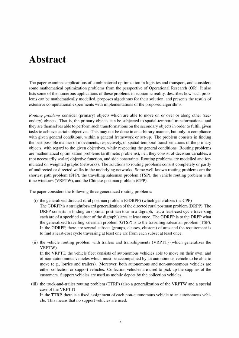
The paper examines applications of combinatorial optimization in logistics and transport, and considerssome mathematical optimization problems from the perspective of Operational Research (OR). It alsolists some of the numerous applications of these problems in economic reality, describes how such prob-lems can be mathematically modelled, proposes algorithms for their solution, and presents the results ofextensive computational experiments with implementations of the proposed algorithms.
Routing problems consider (primary) objects which are able to move on or over or along other (sec-ondary) objects. That is, the primary objects can be subjected to spatial-temporal transformations, andthey are themselves able to perform such transformations on the secondary objects in order to fulfill giventasks to achieve certain objectives. This may not be done in an arbitrary manner, but only in compliancewith given general conditions, within a general framework or set-up. The problem consists in findingthe best possible manner of movements, respectively, of spatial-temporal transformations of the primaryobjects, with regard to the given objectives, while respecting the general conditions. Routing problemsare mathematical optimization problems (arithmetic problems), i.e., they consist of decision variables, a(not necessarily scalar) objective function, and side constraints. Routing problems are modelled and for-mulated on weighted graphs (networks). The solutions to routing problems consist completely or partlyof undirected or directed walks in the underlying networks. Some well-known routing problems are theshortest path problem (SPP), the travelling salesman problem (TSP), the vehicle routing problem withtime windows (VRPTW), and the Chinese postman problem (CPP).
The paper considers the following three generalized routing problems:
(i) the generalized directed rural postman problem (GDRPP) (which generalizes the CPP)The GDRPP is a straightforward generalization of the directed rural postman problem (DRPP). TheDRPP consists in finding an optimal postman tour in a digraph, i.e., a least-cost cycle traversingeach arc of a specified subset of the digraph’s arcs at least once. The GDRPP is to the DRPP whatthe generalized travelling salesman problem (GTSP) is to the travelling salesman problem (TSP):In the GDRPP, there are several subsets (groups, classes, clusters) of arcs and the requirement isto find a least-cost cycle traversing at least one arc from each subset at least once.
(ii) the vehicle routing problem with trailers and transshipments (VRPTT) (which generalizes theVRPTW)In the VRPTT, the vehicle fleet consists of autonomous vehicles able to move on their own, andof non-autonomous vehicles which must be accompanied by an autonomous vehicle to be able tomove (e.g., lorries and trailers). Moreover, both autonomous and non-autonomous vehicles areeither collection or support vehicles. Collection vehicles are used to pick up the supplies of thecustomers. Support vehicles are used as mobile depots by the collection vehicles.
(iii) the truck-and-trailer routing problem (TTRP) (also a generalization of the VRPTW and a specialcase of the VRPTT)In the TTRP, there is a fixed assignment of each non-autonomous vehicle to an autonomous vehi-cle. This means that no support vehicles are used.
ix

Abstract x
Two of these problems, the GDRPP and the VRPTT, are new in the sense that they have not yet beendescribed in the literature, i.e., there are neither formulations nor heuristic or exact solution proceduresfor them.
The problems are generalized in the following sense. Routing problems like the TSP, the VRPTW, andthe CPP are essentially sequencing problems. The difficulty in these problems consists in determiningan optimal sequence of objects. The GDRPP, the VRPTT, and the TTRP involve an additional degreeof freedom: A selection must be made as to which objects to sequence (which primary objects to ‘use’and/or which secondary objects to ‘visit’ or ‘service’) in order to fulfill the given tasks.
The paper is intended to be a contribution to the field of OR. OR is an interdisciplinary field which liesat the interface of business administration, mathematics, and computer science. Hence, the paper strivesto make a three-fold contribution. It covers
(i) the problem- and application-oriented aspect (business administration)The application aspect does not consist in the solution of real-world problem instances or the pre-sentation of case studies, but the practical relevance of the three problems dealt with is emphasizedby the description of actual and potential areas of application and references to pertinent literature.
(ii) the model- and method-oriented aspect (mathematics)The mathematical aspect has a model-oriented and a method-oriented part. The model-orientedpart consists in the (mixed) integer programming formulations developed for the three problemsunder consideration. The method-oriented part consists in the algorithmic treatment of the threeproblems. All problems are solved by branch-and-cut, and the problems are also solved partiallyor completely by dynamic-programming based labelling algorithms using the resource concept.Additionally, several heuristics are developed for the GDRPP, and for the TTRP, a branch-and-price algorithm is proposed.
(iii) the implementation-oriented aspect (computer science)The computer science aspect is covered by sections on computational experiments and a sectionwhere the design and the implementation of a generally usable computer code for solving theshortest path problem with resource constraints are described. The code was developed as part ofthe paper and is used in the computational experiments.

Chapter 1
Introduction
This paper is concerned with applications of combinatorial optimization in logistics and transport, andconsiders some mathematical optimization problems from the perspective of Operational Research (OR).It lists some of the numerous applications of these problems in economic reality, describes how suchproblems can be mathematically modelled, proposes algorithms for their solution, and presents the resultsof extensive computational experiments with implementations of the proposed algorithms.
1.1 Subject Matter
Routing problems consider (primary) objects which are able to move on or over or along other (sec-ondary) objects. That is, the primary objects can be subjected to spatial-temporal transformations, andthey are themselves able to perform such transformations on the secondary objects in order to fulfil giventasks to achieve certain objectives. This may not be done in an arbitrary manner, but only in compliancewith given general conditions, within a general framework or set-up. The problems consist in findingthe best possible manner of movements, respectively, of spatial-temporal transformations of the primaryobjects, with regard to the given objectives, while respecting the general conditions. Routing problemsare mathematical optimization problems (arithmetic problems), i.e., they consist of decision variables,a (not necessarily scalar) objective function, and side constraints. Routing problems are represented onweighted graphs (networks). The solutions to routing problems consist completely or partly of undi-rected or directed walks in the underlying networks.
Examples of routing problems abound. The most common routing problem is the shortest path problem(SPP). This is what an internet router faces when sending packets of data (primary objects), receivedfrom a host computer, to a client machine via a minimal number of ‘hops’ (objective) over other internetrouters (secondary objects) in order to satisfy the client’s request for the information contained in sucha packet (task). The routing problem per se is the famous travelling salesman problem (TSP), where thesalesman is the primary object that is moving in space and time through a road network (roads: sec-ondary objects) in order to visit customers (secondary objects, too) and fulfil their visiting requests (thesalesman’s task) while not wasting time or fuel en route (the salesman’s objective). Another example isthe vehicle routing problem with time windows (VRPTW), where several capacity-constrained vehicles(primary objects) located at a depot visit geographically dispersed customers (secondary objects) duringthe customers’ working hours (conditions) via a road network in order to collect supplies (task) whilenot driving more kilometres than necessary (objective). Yet another example is the Chinese postmanproblem (CPP), where a postman (primary object) traverses the streets in his district (secondary objects)in order to distribute mail (task) while keeping his overall walking distance at a minimum (objective).
This paper considers the following three generalized routing problems:
(i) the generalized directed rural postman problem (GDRPP) (which generalizes the CPP)
1

1.2 Contribution 2
(ii) the vehicle routing problem with trailers and transshipments (VRPTT) (which generalizes theVRPTW)
(iii) the truck-and-trailer routing problem (TTRP) (which also generalizes the VRPTW and is a specialcase of the VRPTT)
The problems are described in detail in the respective chapters. Two of these problems, the GDRPP andthe VRPTT, are new in the sense that they have not yet been described in the literature, i.e., there existneither formulations nor heuristic or exact solution procedures for them.
What is generalized in these problems? Usually, in mathematical optimization, a problem A is said to bea generalization of another problem B if every instance of B constitutes an instance of A. This is the casewhen A considers all aspects relevant in B (and perhaps additional aspects as well; one can then also saythat A is an extension of B). For example, the VRPTW is a generalization of the TSP, because every TSPinstance can be interpreted as a VRPTW instance with one vehicle, where all customers may be visitedat any time and have a supply of zero. In this paper, the word ‘generalized’ has an extended meaning(the term itself is generalized): Routing problems like the TSP, the VRPTW, and the CPP are essentiallysequencing problems. The difficulty in these problems consists in determining an optimal sequence ofobjects/customers/streets. The GDRPP, the VRPTT, and the TTRP involve an additional degree of free-dom: A selection must be made as to which primary objects to ‘use’ and/or which secondary objects tosequence (i.e., to ‘visit’ or ‘service’) in order to fulfil the given tasks. A well-known example where theterm ‘generalized’ is used in this sense is the generalized travelling salesman problem. In this problem,the salesman has several visitation options for each customer (for example, offices of one and the samecustomer in different cities), and he must select one out of these options for each customer and must visitthe selected options in an optimal sequence.
The selection of the problems treated in this paper is a result of the author’s occupational activity inindustry and academia. However, this does not mean that the problems are not of very general relevance.On the contrary: As will be demonstrated, these problems encompass important aspects encountered inmany diverse practical applications that are as multi-faceted as the problems themselves.
1.2 Contribution
The paper is intended to be a contribution in the field of OR. OR is an interdisciplinary field which liesat the interface of business administration, mathematics, and computer science. Hence, the paper strivesto make a three-fold contribution. While covering
(i) the problem- and application-oriented aspect (business administration) by considering problemswhich are relevant in the real world and which are, hence, interesting for practitioners,
(ii) the model- and method-oriented aspect (mathematics) by showing how the problems can be mod-elled, formulated, and solved, and
(iii) the implementation-oriented aspect (computer science/programming) by examining and compar-ing solution algorithms through performing computational experiments,
this paper focuses mainly on the mathematical aspect. The application aspect does not consist in thesolution of real-world problem instances or in the presentation of case studies, but the practical relevanceof the three problems dealt with is emphasized by the description of actual and potential areas of appli-cation and references to pertinent literature. The computer science aspect is covered by the sections oncomputational experiments and by Section 2.4, where the design and the implementation of a computercode for solving the shortest path problem with resource constraints are described.

1.3 Outline 3
The mathematical aspect has a model-oriented and a method-oriented part. The model-oriented part con-sists in the (mixed) integer programming formulations developed for the three problems under considera-tion. The method-oriented part consists in the algorithmic treatment of the three problems. All problemsare solved by branch-and-cut, and the problems are also solved partially or completely by dynamic-programming-based labelling algorithms using the resource concept. Additionally, several heuristics aredeveloped for the GDRPP, and for the TTRP, a branch-and-price algorithm is proposed.
A large part of the results presented in this paper are already contained in Drexl 2005a, Drexl 2005b(Chapter 3), Drexl 2005c (Chapter 4), and Drexl 2006 (Chapter 5).
1.3 Outline
In Chapter 2, the shortest path problem with resource constraints and its solution by labelling algorithmsbased on dynamic programming is considered. The resource concept, as specified in this section, con-stitutes a very powerful framework for the solution of many different kinds of routing problem. Thepresent paper offers pertinent examples. Indeed, a central topic of this paper is the evaluation of the pos-sibilities and limitations of dynamic-programming-based labelling algorithms for the solution of routingproblems. Chapter 3 is concerned with the generalized directed rural postman problem (GDRPP); inChapters 4 and 5, the vehicle routing problem with trailers and transshipments (VRPTT) and the truck-and-trailer routing problem (TTRP) are treated respectively. For each of the three problems being dealtwith, different formulations are given, solution algorithms are developed, and computational experimentsare presented and analyzed. Chapter 6 outlines the numerous possible lines of research on the GDRPP,the VRPTT, and the TTRP that could not be pursued in this paper.
1.4 Mathematical Prerequisites, Terminology, and Notation
The material covered in this paper, and the exposition thereof, require knowledge of the standard ORmodelling and algorithmic techniques used to address problems of logistics and transport. Since manytextbooks covering these prerequisites are available, the fundamentals are not repeated once again here.However, the central problem and the central algorithmic technique used throughout the paper, the (el-ementary) shortest path problem with resource constraints and its solution via a labelling algorithm, istreated in detail, not least because the resource concept used in labelling algorithms is, as yet, not a stan-dard topic in OR textbooks.
The problems particularly relevant for this paper are shortest path problems with and without resourceconstraints (SPPs), uncapacitated arc routing problems (ARPs), travelling salesman problems (TSPs),and vehicle routing problems (VRPs). Standard references are Ahuja et al. 1993, p. 93 ff. (SPPs), Assad/Golden 1995, Eiselt et al. 1995a, Eiselt et al. 1995b, Dror 2000b (ARPs), Lawler et al. 1985, Gutin/Punnen 2002 (TSPs), Toth/Vigo 2002 (VRPs).
As for the algorithmic side, familiarity with graph theory and linear and mixed integer programming isnecessary. In particular, knowledge of the Dijkstra algorithm for the SPP and of the branch-and-cut andthe branch-and-price algorithmic principles is assumed. Recommendable textbooks are Volkmann 1996,West 1996 (graph theory), Dantzig 1963, Chvatal 1983, Murty 1983 (linear programming), Sierksma1996, Wolsey 1998, Martin 1999 (mixed integer programming). Standard references for branch-and-price are Barnhart et al. 1998, Vanderbeck 2000, Desrosiers/Lubbecke 2005, Lubbecke/Desrosiers 2005.Desaulniers et al. 1998 present a unified model for the solution of time-constrained vehicle routing andscheduling problems by branch-and-price.
Additionally, basic knowledge of complexity theory and data structures and algorithms is useful (Ahoet al. 1983, Sedgewick 1992).

1.4 Mathematical Prerequisites, Terminology, and Notation 4
Textbooks covering the basic problems as well as the methods relevant for this paper are Domschke1995, Domschke 1997, Bramel/Simchi-Levi 1997. The excellent books Grunert/Irnich 2005a, Grunert/Irnich 2005b are particularly recommendable.
The term formulation is used to denote a concrete algebraic representation of a model of a problem. Torepresent the data defining a problem instance, systems of sets and functions representing properties ofthe elements of the sets are used. Such functions are called attributes. Throughout, for a function f , theindex notation fi is used for the value f (i). M is a ‘sufficiently large’ positive constant.
G = (V, L) denotes a graph with vertex set V and link set L . The relationship between V and L isestablished via two functions, ta : L → V , the tail function, and he : L → V , the head function. taa
is called tail of a, and hea is called head of a. A link l with tal = hel is called loop. All consideredgraphs are assumed to be loop-free w.l.o.g. Links l that may be traversed in either direction, i.e., fromtal to hel and vice versa, are called edges; links l that may be traversed only from tal to hel are calledarcs. Where there is no danger of confusion, the notations (taa, hea) and taahea are used to denote anarc a by its tail and head. Graphs containing only edges are called undirected graphs and are denotedby G = (V, E). Graphs containing only arcs are called directed graphs or digraphs and are denotedby D = (V, A). Graphs containing edges as well as arcs are called mixed graphs. Mixed graphs are ageneralization of undirected and directed graphs. For any graph G = (V, L), L := E ·∪ A, where E(A) is the edge (arc) set of G, i.e., the set of links that can be traversed in both directions, and the set oflinks that can only be traversed from tail to head respectively. Two edges e, e′ ∈ E are called parallelif {tae, hee} = {tae′, hee′}; two arcs a, a′ ∈ A are called parallel if taa = taa′ and hea = hea′ . A graphwithout loops and without parallel links is called simple. All graphs considered in this paper are simpledigraphs unless otherwise specified. Digraphs with an arc attribute representing costs of traversal arealso referred to as networks. Given a digraph D = (V, A), for each V ′ $ V , the forward (backward)star of V ′ is the set {a ∈ A : taa ∈ V ′ 63 hea} ({a ∈ A : taa 6∈ V ′ 3 hea}).
Given a graph G = (V, L), S := (i0, l1, i1, l2, i2, l3, . . . , ip−1, lp, ip) is called link sequence if iq ∈
V, q = 0, . . . , p, lq ∈ L , q = 1, . . . , p, {talq , helq } = {iq−1, iq}, q = 1, . . . , p. If S is a link se-quence, it is called closed if i0 = ip and open otherwise, and it is called walk or non-elementary pathif lq ∈ A implies talq = iq−1, q = 1, . . . , p. A walk is called directed if all of its links are arcs. A(directed) walk is called (directed) trail if no link (arc) appears twice in the walk, i.e., if q 6= q ′ implieslq 6= lq ′, q, q ′ = 1, . . . , p. An open (directed) trail is called (directed) (elementary) path if no vertexappears twice in the trail, i.e., if q 6= q ′ implies iq 6= iq ′, q, q ′ = 0, . . . , p; this implies that no link(arc) appears twice. A closed (directed) trail is called (directed) cycle. It is assumed throughout that allconsidered (di)graphs are (strongly) connected, i.e., that there is a (directed) walk between any pair ofvertices. Given a link traversal cost attribute of the form c : L → R, the length or costs cS of a walk Sis/are equal to the sum of the traversal costs of the links in S in the direction the links are traversed in S.S := (i0, . . . , ip) is a shortest walk if cS 5 cS′ for all walks S′ from i0 to ip. Independent of the meaningof c, a closed directed trail S with cS 5 0 (cS < 0) is called non-positive (negative) cycle (with respect toc) or, if the textual denomination of the attribute is attr, non-positive (negative) attr cycle. Note that it isusual in the literature to use the term ‘shortest’ walk, independent of the actual meaning of the attribute c,i.e., walks with minimal cS value are referred to as ‘shortest’ even if c denotes costs or time or somethingelse.

Chapter 2
Resource-Constrained Shortest Paths andLabelling Algorithms
The shortest path problem with resource constraints (SPPRC) seeks a shortest (cheapest, ‘best’) path ina network with arbitrary arc lengths (costs) from an origin vertex o to a destination vertex d subject toone or more ‘resource constraints’. For example, one might seek a path of minimal length from o to dsubject to the constraints that
• the total travel time must not exceed some upper bound and/or
• the total amount of some good that has to be collected at the vertices along the path be less than orequal to some capacity limit and/or
• if two vertices i and j are visited on a path, then i must be visited before j .
The SPPRC and its solution by a ‘labelling algorithm’ based on dynamic programming constitute a cen-tral topic of this paper. In actual fact, however, there is no such thing as the SPPRC; rather, SPPRCsare a general framework: Many different problems can be viewed and modelled as (special types of)resource-constrained shortest path problem(s).
The next section describes the workings of labelling algorithms. To illustrate the presented concepts,Section 2.2 provides a detailed numerical example. Section 2.3 discusses the issue of negative cyclesin SPPRCs and their implications for the complexity of the problem. Section 2.4 describes a genericsoftware framework for the solution of SPPRCs, which was written as part of this paper.
2.1 Labelling Algorithms
A labelling algorithm is the solution method of choice for SPPRCs. It works similarly to a labellingalgorithm for shortest path problems without resource constraints (SPPs), e.g., the Dijkstra algorithm(cf. Ahuja et al. 1993, p. 93 ff.). The basic concepts used in a labelling algorithm for SPPRCs are thefollowing (cf. Irnich/Desaulniers 2005):
• A resource is an arbitrarily scaled one-dimensional quantity that is consumed when moving alongthe arcs and whose consumption can be measured or computed at the vertices of a directed walkin a network. Examples are cost, time, load, or an information such as ‘Has lorry k already visitedcustomer i?’ or ‘Is lorry k currently pulling its trailer?’. The value of a resource at a vertex isstored in a resource variable. An arbitrarily scaled resource is constrained if there is at least onevertex in the network where the associated resource variable must not take all possible values. Acardinally scaled resource is constrained if there is at least one vertex in the network with a finiteupper or lower bound on the value of the resource. The resource window of a nominally scaledresource r at a vertex is the set of allowed values of r at this vertex. The resource window of acardinally scaled resource r at a vertex i is the interval [lbr
i , ubri ] j ]−∞,+∞[.
5

2.1 Labelling Algorithms 6
• A resource extension function (REF) is defined on each arc in a network for each resource con-sidered. An REF for a resource r maps the set of all possible vectors of resource values atthe tail of an arc to the set of possible values of r at the head of the arc. More precisely, letR := (σ 1, . . . , σ |R|)T be a vector of (values of) resource variables. Then, an REF for a resourcer is a function f r : A × R|R| → R. For simplicity, let f r
i j (R) := f r (((i, j), R)). An REF for acardinally scaled resource r indicates lower bounds on the consumptions of r along the arcs. Whenseeking a path from an origin vertex o to a destination vertex d , partial paths from o to a vertexi 6= d are extended along all arcs (i, j) emanating from i to create new, extended paths.
• For each o-i-path, there is a corresponding label l resident at i that stores the values of all resourcevariables at i for its path, along with the information on how it was created: the arc (h, i) overwhich i was reached and (a reference to) the label of the o-h-path whose extension along (h, i)yielded the o-i-path. (This makes it easy to reconstruct the path corresponding to a label.) Initially,there is exactly one label corresponding to the path (o). For nominally scaled resources, the valuesof the resource variables of the initial label are an input to the labelling algorithm. For cardinallyscaled resources, the values of the resource variables of the initial label are w.l.o.g. all set to thelower bounds of their respective resource windows at o. A label l is feasible if and only if thevalue of each resource variable in l is within the resource window of its respective resource. If alabel is not feasible, it is discarded. An extension of a path/label along an arc (i, j) is feasible if theresulting label at j is feasible. An h- j-path is feasible if, for each arc (i, i ′) in the path, a feasiblelabel at i exists which can be extended along (i, i ′) to a feasible label at i ′.
• To keep the number of labels as small as possible, it is decisive that a dominance procedure beperformed to eliminate feasible but unnecessary labels. A label l dominates a label l ′ if both resideat the same vertex, if the value of the resource variable of each nominally scaled resource in lis equal to the corresponding value in l ′, if the value of the resource variable of each cardinallyscaled resource in l is ‘better’ (less or greater, depending on the resource) than or equal to thecorresponding value in l ′, and if the value of the resource variable of at least one cardinally scaledresource in l is strictly ‘better’ than the corresponding value in l ′. A path p dominates a path p′ ifthe label corresponding to p dominates the label corresponding to p′. Dominated paths/labels arediscarded as well. An undominated path/label is called Pareto-optimal. A dominance procedurethat always compares one label with one other label performs pairwise dominance. Pairwise dom-inance relationships are transitive. It is sometimes also possible and useful to devise dominanceprocedures for non-pairwise dominance, where it is checked whether a set of labels dominates oneother label.
A labelling algorithm for an SPPRC consists of the following five basic steps:
(i) InitializationThe algorithm maintains a set of unprocessed labels. As mentioned above, the algorithm is initial-ized with a first label resident at o. This label is added to the set of unprocessed labels.
(ii) Label selectionAn unprocessed label is selected from the set of unprocessed labels as a candidate for extension.
(iii) DominanceOnly undominated labels should be extended. Hence, before a label is extended, it should bechecked whether the label is dominated or not. Different strategies for dominance are possible, andthe dominance check can be performed at different points in the algorithm. In any case, it shouldbe ensured that the check is performed as efficiently as possible. In particular, no dominance checkshould be performed more than once, and no redundant dominance check should be performed atall.
(iv) Label extensionThe path corresponding to a label is extended along each arc in the forward star of the end vertex

2.2 A Concrete Example: the Shortest Path Problem with Time Windows 7
of the path (the resident vertex of the label), i.e., for each forward star arc, a new label is createdat the end vertex of the arc, and the values of the resource variables of the new label are computedby applying the REFs. Each new label is checked for feasibility. If it is feasible, it is added to theset of unprocessed labels.
(v) Solution selectionAt the end of the algorithm, if the desired destination vertex could be reached, it must be decidedwhich Pareto-optimal solution(s) (undominated label(s) resident at the destination vertex and thecorresponding path(s)) should be returned.
2.2 A Concrete Example: the Shortest Path Problem with Time Windows
The easiest example of an SPPRC is the shortest path problem with time windows (SPPTW). It can bedefined on a simple digraph D = (V, A) with a cost function c : A→ Z, an arc traversal time functionτ tr : A→ Z+, and vertex time windows tw : V → {[a, b] : a, b ∈ [0, T max ], a 5 b} with T max
∈ Z+.[ai , bi ] is used in this chapter to denote the time window of vertex i ∈ V . Given an origin vertex o ∈ Vand a destination vertex d ∈ V , the task in the SPPTW is to determine a shortest path from o to d thatrespects the vertex time windows of all vertices in the path. Respecting vertex time windows means thatthe arrival time at any vertex i is not later than the respective right time window bound bi . Arrival beforethe left time window bound ai (‘waiting’) is allowed; the arrival time at a vertex i is simply assumed tobe always later than or equal to ai . This problem can be formulated as a mixed-integer programmingproblem as follows:
(SPPTW): ∑(i, j)∈A
ci j xi j→ min subject to (2.1a)
∑{h∈V :(h,i)∈A}
xhi −∑
{ j∈V :(i, j)∈A}
xi j=
−1, i = o
1, i = d0, otherwise
(2.1b)
xi j = 1⇒ ti + τ tri j 5 tj ∀ (i, j) ∈ A (2.1c)
xi j ∈ {0, 1} ∀ (i, j) ∈ A (2.1d)
ai 5 ti 5 bi ∀ i ∈ V (2.1e)
(2.1c) are equivalent to the linear constraints
ti + τ tri j − tj 5 M(1− xi j ) ∀ (i, j) ∈ A. (2.1c′)
In the SPPTW, two resources have to be considered:
(i) an unconstrained, cardinally scaled resource for cost, and
(ii) a constrained, cardinally scaled resource for time.
For cost, the resource r cost with resource variable σ costi (indicating the value of the cost resource at vertex
i) and REF f rcostwith
f rcost
i j (σ costi ) = σ cost
i + ci j (2.2)
can be used.
For time, the resource r time with resource variable σ timei and REF f r time
with

2.2 A Concrete Example: the Shortest Path Problem with Time Windows 8
f r time
i j (σ timei ) = max{ai , σ
timei + ti j } (2.3)
can be used. The resource window at a vertex i is [ai , bi ].
Usually, in a labelling algorithm, the cost REF models the objective function of an MIP model, and theREFs for resources other than cost correspond to the constraints.
What about dominance? Applying the definition given in the previous section and denoting by σ r (l)the (value of the) resource variable of resource r for a label l, the dominance relationship for two la-bels l, l ′ is as follows. l dominates l ′ if and only if both reside at the same vertex, σ cost(l) 5 σ cost(l ′),σ time(l) 5 σ time(l ′), and at least one of the two inequalities is strict. To understand why it is importantto consider all resources in the dominance check, consider the network in Figure 2.1. It is easy to seethat the shortest feasible path from o to d is (o, a2, j, a4, i, a3, d). There are two paths from o to i :p1 := (o, a1, i) with costs of 2 and an arrival time at i of 3, and p2 := (o, a2, j, a4, i) with costs of 3 andan arrival time at i of 2. If there are no time windows, path p2 can be discarded, because p1 is shorter (haslower costs) and thus its extension to d is shorter (cheaper) than the extension of p2: p1 dominates p2.However, with the time windows indicated in the figure, p1 cannot be extended to d , because the arrivaltime at d of the extended path is 5, which is later than the right time window bound of d . The extensionof p2 to d , by contrast, is possible: The arrival time of the extended path at d is 4, which lies within d’stime window. The only other o-d-path, p3 := (o, a2, j, a5, d) has costs of 7 and an arrival time at d of 3.Thus, if a shortest (i.e., cheapest) path from o to d is sought, discarding path p2 by judging only by costleads to a sub-optimal solution. If p3 were also infeasible, no feasible solution at all would be discovered.The decisive point is that paths p1 and p2 (equivalently, their corresponding labels) are incomparable. p1
is ‘better’ with respect to costs, p2 is ‘better’ with respect to time. So, neither does p1 dominate p2, be-cause for any extension of p1, the arrival time at the last vertex of the corresponding extension of p2 is notlater, nor does p2 dominate p1, because for any extension of p2, the costs of the corresponding extensionof p1 are lower. Neither path is ‘better’ than the other one; both paths are undominated or Pareto-optimal.
ss
sso
[0, 0]
i[2, 4]
j[1, 5]
d[3, 4]
..............................................................................................................................................................
...................................................................................................................................................... ........
..................................................................................................................................................... ........
........
........
........
........
........
........
........
........
........
........
........
........
........
........
........
........
........
........
........
........
........
........
........
........
........
........
.................
.............................................................................................................................................................
a1(2, 3)
a2(2, 1)
a3(2, 2)
a4(1, 1)
a5(5, 2)
[a, b]: Time window(c, t) : Costs and traversal time
Figure 2.1: Example of an SPPTW
What is still needed is a rule for the selection of a label to be extended. The easiest rule is the FIFO rule:Add the labels to and remove them from the set S of unprocessed labels in the order that they are created.Many other strategies exist.
A labelling algorithm for the SPPTW can now be described as follows:
SPPTW-Labelling:Given: a digraph D = (V, A) constituting an SPPTW instance; origin and destination vertices o ∈ Vand d ∈ V ; an empty set of unprocessed labels S; for each vertex i ∈ V , an empty set of labels residentat i .Create an initial label l0 at o with σ cost(l0) := 0, σ time(l0) := ao, predecessor arc := −, and predecessorlabel := −.
2.2 A Concrete Example: the Shortest Path Problem with Time Windows 9
Insert l0 into the set S of unprocessed labels.While S is not empty:
Select and remove a label lcurr from S according to the FIFO rule.Perform a dominance check for all labels resident at the vertex i where lcurr resides.Mark all dominated labels as dominated.Delete all labels which are both dominated and processed.If lcurr is not dominated:
Mark lcurr as processed.For each arc (i, j) in the forward star of i , the vertex where lcurr resides:
Extend lcurr along (i, j) to a new label lnew by applying REFs (2.2) and (2.3).If lnew is not feasible
Delete lnew.else
Insert lnew into S.Insert lnew into the set of labels resident at j .
elseDelete lcurr .
If d could be reached from o:For each label l resident at d:
Decide whether to return l as a Pareto-optimal solution; if so, recursively construct the cor-responding Pareto-optimal o-d-path.
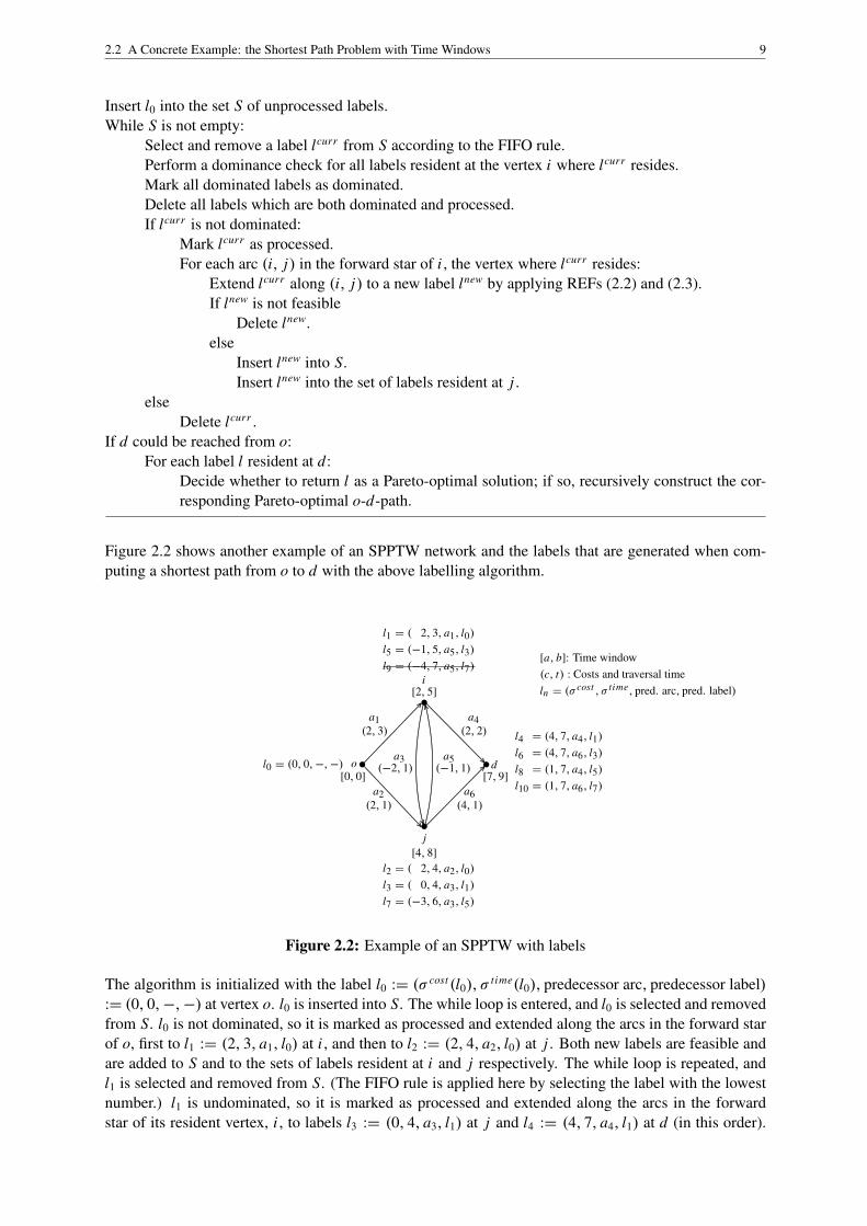
Figure 2.2 shows another example of an SPPTW network and the labels that are generated when com-puting a shortest path from o to d with the above labelling algorithm.
ss
sso
[0, 0]l0 = (0, 0,−,−)
i[2, 5]
l1 = ( 2, 3, a1, l0)
l5 = (−1, 5, a5, l3)
l9 = (−4, 7, a5, l7)
j[4, 8]
l2 = ( 2, 4, a2, l0)
l3 = ( 0, 4, a3, l1)
l7 = (−3, 6, a3, l5)
d[7, 9]
l4 = (4, 7, a4, l1)
l6 = (4, 7, a6, l3)
l8 = (1, 7, a4, l5)
l10 = (1, 7, a6, l7)
.............................................................................................................................................................
...................................................................................................................................................... ........
...................................................................................................................................................................................................................................
......................................................................................................................................................... ........
.....................................................................................................................................................................................................................................
.................................................................................................................................................................
a1(2, 3)
a2(2, 1)
a3(−2, 1)
a4(2, 2)
a5(−1, 1)
a6(4, 1)
[a, b]: Time window(c, t) : Costs and traversal timeln = (σ cost , σ time, pred. arc, pred. label)
Figure 2.2: Example of an SPPTW with labels
The algorithm is initialized with the label l0 := (σ cost(l0), σtime(l0), predecessor arc, predecessor label)
:= (0, 0,−,−) at vertex o. l0 is inserted into S. The while loop is entered, and l0 is selected and removedfrom S. l0 is not dominated, so it is marked as processed and extended along the arcs in the forward starof o, first to l1 := (2, 3, a1, l0) at i , and then to l2 := (2, 4, a2, l0) at j . Both new labels are feasible andare added to S and to the sets of labels resident at i and j respectively. The while loop is repeated, andl1 is selected and removed from S. (The FIFO rule is applied here by selecting the label with the lowestnumber.) l1 is undominated, so it is marked as processed and extended along the arcs in the forwardstar of its resident vertex, i , to labels l3 := (0, 4, a3, l1) at j and l4 := (4, 7, a4, l1) at d (in this order).

2.3 Negative Cycles, Elementary Paths, and Complexity 10
Both new labels are feasible and are added to S and to the sets of labels resident at j and d respectively.Next, l2 is selected and removed from S. The dominance check at vertex j , l2’s resident vertex, yieldsthe result that l2 is dominated by l3, which has the same arrival time but a lower cost. Therefore, l2 isdeleted. After that, l3 is selected and removed from S. It is currently the only label resident at j , andit is not dominated, so it is marked as processed and extended along the arcs in the forward star of j tol5 := (−1, 5, a5, l3) at i and l6 := (4, 7, a6, l3) at d (in this order). Both new labels are feasible and areadded to S and to the sets of labels resident at i and d respectively. l4 is the next label that is selected andremoved from S. It is undominated, so it is marked as processed. It is not extended, because there are noarcs emanating from d . The next label to be selected and removed from S is l5. The dominance check ati yields the result that all labels at i (l1 and l5) are undominated. Hence, l5 is marked as processed andextended to the feasible labels l7 := (−3, 6, a3, l5) at j and l8 := (1, 7, a4, l5) at d (in this order). Again,both new labels are feasible and are added to S and to the sets of labels resident at j and d respectively. l6
is the next candidate label for extension, but it is dominated by l8 and is therefore deleted, together withl4. Now, l7 is selected and removed from S. The dominance check at j yields no dominance relationshipbetween the two existing labels (l3 and l7). l7 is marked as processed and extended to l9 := (−4, 7, a5, l7)
at i and l10 := (1, 7, a6, l7) at d. l9 is not feasible and is deleted. l10 is feasible and is added to S and tothe set of labels resident at d . l8 is the next label to be selected and removed from S. l8 is not dominated,so it is marked as processed. It cannot be extended. The last label to be selected and removed from S isl10. It is undominated and cannot be extended either. The while loop ends. d could be reached from o.The labels resident at d are l8 and l10. Both have the same values for costs and time, but they correspondto different paths. The predecessor label of l8 is l5, whose predecessor label is l3, whose predecessorlabel is l1, whose predecessor label is l0, so the path corresponding to l8 is (o, a1, i, a3, j, a5, i, a4, d).Similarly, the path corresponding to l10 is (o, a1, i, a3, j, a5, i, a3, j, a6, d). Both Pareto-optimal pathsare non-elementary. The shortest feasible elementary path is (o, a2, j, a5, i, a4, d).
2.3 Negative Cycles, Elementary Paths, and Complexity
A subtle difficulty with the above algorithm is that it does not compute shortest elementary paths, itcomputes shortest walks. When the underlying network does not contain any non-positive cost cycles,all undominated walks will be elementary paths. In the presence of negative cost cycles, there may beundominated non-elementary paths (see the above example). However, the algorithm will still be finiteunless there is a non-positive time cycle. If there are both non-positive cost and time cycles, the algo-rithm may enter an infinite loop. For SPPRCs on general networks, this means that, in order to avoidsuch difficulties, it must be required that there be no non-positive cost cycles or at least one resourcewithout non-positive cycles.
Formulation (2.1) is not valid if the traversal time function is τ tr : A → Z. Subtour elimination con-straints involving only arc variables are necessary in this case; constraints (2.1c) are no longer sufficient.In addition, to require elementarity of paths, the constraints∑
{ j∈V :(i, j)∈A}
xi j 5 1 ∀ i ∈ V (2.4)
are necessary.
If there is at least one cycle with a resource consumption of zero for all considered resources, but nonegative cycle for any of them, a label counter resource can be added to ensure finiteness: The labels arenumbered consecutively in increasing order, and in the dominance check, if two labels have equal valuesfor all other resources, the label with the lower number dominates the other one.
To solve the elementary SPPRC (ESPPRC) on general networks, Feillet et al. 2004 have extended anidea first presented in Beasley/Christofides 1989: the introduction of a binary resource for each vertex

2.4 The r c shortest paths Framework 11
(a visitation counter) indicating whether the vertex can still be visited. Partial paths are only extended inaccordance with the visitation counter resources, and a path p1 dominates a path p2 only if p1 can stillvisit any vertex that p2 can. Their approach is used in this paper for the solution of the pricing problemsin the branch-and-price approach for the TTRP and is described in detail in Chapter 5; in addition, thelabelling algorithm used for solving the GDRPP in Chapter 3 is also based on visitation counter resources.
As far as the computational complexity of SPPRCs is concerned, it can be shown that they are, in general,N P-hard, but on networks without negative cycles, or when the paths need not be elementary, SPPRCscan be solved in pseudopolynomial time (the above algorithm is such a one for the SPPTW). However,the ESPPRC on general networks is N P-hard in the strong sense (Dror 1994); no pseudopolynomialalgorithms are known.
The shortest path problem without resource constraints (SPP) (which corresponds to formulation 2.1a,b,d)is a special SPPRC with only one resource, the unconstrained resource ‘cost’. The SPP is interesting froma computational complexity point of view, as it shows that the ‘hardness’ of a problem does not necessar-ily depend on the problem type or the instance size; it may also depend on the instance data: The SPP onnetworks with positive arc cost function is polynomially solvable; on general networks, it is N P-hard(Garey/Johnson 1979, p. 213).
2.4 The r c shortest paths Framework
As a part of this paper, a small framework for the solution of (E)SPPRCs was developed and implementedin C++ according to the paradigm of generic programming. The framework was accepted for inclusioninto the Boost Graph library (BGL) and will be part of its 1.35.0 release. Boost (boost.org) is anonline community that encourages development and peer review of free C++ libraries. This sectiondescribes the developed framework. Familiarity with the C++ programming language and the StandardTemplate Library (STL) is assumed. The section is rather technical, but the rest of the paper does notrequire knowledge of the material presented in the remainder of this chapter.
2.4.1 Fundamental Principles of Generic Programming
This subsection briefly reviews the main ideas of generic programming in the context of C++. Genericprogramming (GP) means programming with types as parameters (cf. Stroustrup 1998, p. 349). GPis ‘a methodology for program design and implementation that separates data structures and algorithmsthrough the use of abstract requirement specifications’ (Siek et al. 2002, p. 19).
Important terms in generic programming are (cf. ib.):
• A concept is a set of requirements which a template argument must fulfil so that the class orfunction template will be compiled and executed correctly. Concepts are usually documented insource code comments or an external documentation. Instead of writing down the specification fora single type, a family of types is described, all of which have a common interface and semanticbehaviour. Algorithms constructed in the generic style are applicable to any type that satisfies therequirements of the algorithm. The difference between a class and a concept is that a class is a sin-gular, concrete data type with a unique interface, whereas a concept represents the commonalitiesof a set of types that may otherwise be completely different.
• A model describes the relationship between concrete types and the concepts fulfilled by them.
• A refinement is a concept which extends the requirements of another concept.
Sets of requirements of a concept are (ib., p. 28):
• Valid expressions: Expressions that must compile successfully in order for the types appearing inthe expressions to be considered a model of the concept.

2.4 The r c shortest paths Framework 12
• Associated types: Auxiliary types related to a type modelling a concept.
• Invariants: Run-time characteristics of types that must be fulfilled at any time.
• Complexity guarantees: Worst and average case guarantees with respect to running time and mem-ory requirements.
A central idea in software engineering is polymorphism, which means the ability to use many differenttypes with the same variable or function parameter. There are two types of polymorphism:
(i) Subtype polymorphism:In object-oriented programming (OOP), polymorphism is realized by virtual functions, inheritance(and overloading). Interface requirements of a concept are specified by (pure) virtual functions inan abstract base class. The concrete types which are derived from the abstract base class are calledsubtypes.
(ii) Parametric polymorphism:In generic programming, polymorphism is realized through class or function templates (and over-loading).
Subtype polymorphism uses run-time dispatch of function calls; parametric polymorphism uses compile-time dispatch. Whereas the former is sometimes (virtually) indispensable, the latter is more efficient,which is decisive in lower-level software components, such as mathematical algorithms. Note, however,that OOP and GP are complementing techniques, not competing ones.
2.4.2 Implementation Details
The implementation is designed for use with the Boost Graph library (BGL) (boost.org/libs/-graph/doc/table of contents.html). The BGL is a free, non-commercial, header-only li-brary providing some general purpose graph classes and algorithms via a generic interface. Any graphlibrary that implements this interface will be interoperable with the BGL generic algorithms and withother algorithms that also use this interface.
The implementation consists of overloaded template functions called r c shortest paths and sev-eral underlying concepts.
The concepts are:
• ResourceContainerA type modelling the ResourceContainer concept is used to store the values of the resource vari-ables of a label. It must be a refinement of the Assignable, LessThanComparable, and Equality-Comparable concepts.
• LabelThis concept defines the interface for a label in the r c shortest paths functions. As a designdecision, the functions were not parameterized on the type of label. A concrete type parameterizedon the graph and resource container type is used in the implementation. It stores the predecessorinformation necessary for reconstructing a path at the end of the algorithm.
• ResourceExtensionFunctionA model of the ResourceExtensionFunction concept specifies how a label is extended along an arc.A type modelling this concept is likely to be a function or a function object.
• DominanceFunctionA model of DominanceFunction is used to specify a dominance relation between two labels. Atype modelling this concept will also probably be a function or a function object.

2.4 The r c shortest paths Framework 13
• ResourceConstrainedShortestPathsVisitorA design pattern extensively used in the BGL is that of an algorithm visitor. This is a generalizationof the function object parameter used in many STL functions. An algorithm visitor for a BGLalgorithm defines several functions that are called at certain event points during the algorithm.The ResourceConstrainedShortestPathsVisitor concept defines the visitor interface for the r c -shortest paths functions. The user can define a type with this interface and pass an objectof this type to the r c shortest paths functions in order to perform user-defined actions atthe event points of the algorithm. The event points are when a label is selected and removed fromthe set of unprocessed labels, when a new label is known to be feasible or infeasible, and when alabel is known to be dominated or undominated. A visitor can be used, for example, to count thenumber of generated labels for statistical comparisons or to mark a label as dominated accordingto information from outside the algorithm.
The functions are templated on the graph, resource container, resource extension function, dominance,label memory allocator and algorithm visitor type. There is a default type for the label memory allocatortype and for the algorithm visitor type. Experience shows that, for ‘small’ resource containers, it may beuseful to try a specialized small object allocator. For larger resource containers (i.e., for a large numberof resources), the default allocator is the right choice.
The functions receive a graph object, an origin and a destination vertex, objects for resource extensionand dominance, and containers where the solution is stored (Pareto-optimal labels and their correspond-ing paths). There are two optional parameters: one for an algorithm visitor object, and one for an objectfor allocating the memory for the labels.
It was a design decision not to parameterize the functions on the type of the container storing the setof unprocessed labels. Two different data structures were tried. The version submitted to Boost uses apriority queue. Another version of the functions uses buckets. The bucket version was approximately10–40 % faster than the priority queue version. However, the priority queue version offers a simplerinterface and is more generic. (To use buckets, there must be an integer-valued resource with strictlypositive resource consumption. This resource need not be constrained, but an upper bound for its maxi-mal value at any vertex must be known.)
The framework leaves a lot of work to the user. This, however, is a property inherent to the SPPRC. It isentirely up to the user to make sure that he stores the ‘right’ resources in his resource container object,that the resource extension function extends a label in the desired way, and that the dominance functiondeclares the ‘right’ labels as dominated and not dominated.
The r c shortest paths framework has been used to solve SPPs, SPPTWs, GDRPPs, and numer-ous variants of SPPRC and ESPPRC pricing problems in branch-and-price algorithms for the VRP, theVRPTW, and the TTRP. The framework has been used in the computational experiments described inChapters 3 and 5.
Chapter 3
The Generalized Directed Rural PostmanProblem
This chapter is concerned with the generalized directed rural postman problem (GDRPP). This problemhas not yet been described in the literature, i.e., there are neither formulations nor heuristic or exact solu-tion procedures, but, as its name implies, the problem is a straightforward generalization of the directedrural postman problem (DRPP). The DRPP consists in finding an optimal postman tour in a digraph, i.e.,a least-cost cycle traversing each arc of a specified subset of the digraph’s arcs at least once. The GDRPPis, to the DRPP, what the generalized travelling salesman problem (GTSP) is to the travelling salesmanproblem (TSP): In the GDRPP, there are several subsets (groups, classes, clusters) of arcs and the require-ment is to find a least-cost cycle traversing at least one arc from each subset at least once. The subsetsneed neither be a partition of the arc set, nor need they be disjoint. The GDRPP is an interesting problemin its own right, but it is also important because many uncapacitated routing problems, especially arcrouting problems (ARPs), can be modelled as GDRPPs. Moreover, there are several practically relevantconstraints (e.g., turn penalties) which can be considered when modelling a problem as a GDRPP. Hence,the aim of the current chapter is to present formulations and solution procedures for the GDRPP as wellas transformations of routing problems into GDRPPs, taking into account practically relevant constraints.
The chapter is structured as follows. In Section 3.1, some additional notation used in this chapter isintroduced. In Section 3.2, integer programming formulations for the DRPP and the GDRPP are pre-sented. The proposed transformations are described in Section 3.3, followed by solution procedures forthe GDRPP in Section 3.4 and computational experiments in Section 3.5. The chapter ends with a briefconclusion. The relevant literature is discussed in the respective sections.
3.1 Notation
The graphs considered in this chapter need not be simple, as is usual in the arc routing context. Given anundirected, directed, or mixed graph G = (V, L), c : L → Z+ is a function denoting the length or thecosts of traversal of a link. A graph G = (V, L) is called windy if, instead of c, there are two functions→c : L → Z+ ·∪ {∞} and ←c : L → Z+ ·∪ {∞} denoting the costs of traversal of a link from tail to head andfrom head to tail respectively. As the costs of traversal in one direction may be infinite, windy graphs area generalization of mixed graphs.
Given a graph G = (V, L), two arcs a, a′ ∈ A are called antiparallel if taa = hea′ and hea = taa′ . Fora given subset V ′ j V , L(V ′) is the link set of the vertex-induced subgraph of G induced by V ′. Like-wise, for a given subset L ′ j L , V (L ′) is the vertex set of the link-induced subgraph of G induced by L ′.Furthermore, let H EL ′ := {i ∈ V : ∃ a ∈ L ′ with hea = i}, and let T AL ′ be defined accordingly for tails.
14

3.1 Notation 15
For graphs G = (V, L) with turn penalties, there is a set T of possible turns, and there are three func-tions il : T → L , called inlink function, ol : T → L , called outlink function, and tv : T → V ,called turnvertex function. tv fulfils tvt ∈ {tailt , heilt } ∩ {taolt , heolt } for each t ∈ T . Hence, a turnt ∈ T can be denoted by (ilt , tvt , olt). A graph with turn penalties is denoted by G = (V, L , T ).pet : T → [0,∞] is the turn penalty function, and a turn t with pet <∞ (pet = ∞) is allowed (forbid-den). S := (i0, l1, t1, l2, t2, l3, t3, . . . , lp−1, tp−1, ip, lp) is called walk if i0 ∈ {tal1, hel1} \ {tvt1} ∧ ip =
tvtp−1 ∧ lq ∈ L , q = 1, . . . , p ∧ iltq = lq ∧ oltq = lq+1, q = 1, . . . , p − 1. The length or costs of awalk S in a graph with turn penalties is/are equal to the sum of the traversal costs of the links in S in thedirection the links are traversed in S plus the sum of the penalties of the turns in S minus the traversalcosts of the last link in S in the direction the link is traversed in S. A walk is feasible if it performs noforbidden turns. The other terms defined so far for graphs without turn penalties apply analogously.
For ‘generalized’ problems on a graph G = (V, L), with or without turn penalties, there are pL groupsLq j L , q = 1, . . . , pL , of links, and pV groups Vq j V , q = 1, . . . , pV , of vertices, whereof atleast one element must be traversed/visited in any feasible solution. Such groups are referred to here-after as r-groups, and the links (vertices) belonging to or covering an r-group are called r-group links(r-group vertices). W.l.o.g., it is assumed that every vertex is incident to an r-group link and that alllinks not belonging to an r-group are arcs. For graphs without turn penalties, it is assumed w.l.o.g. thatthere are no parallel links covering the same r-groups and no parallel non-r-group links. A link/vertexthat will be traversed/visited in any optimal solution is called required. For simplicity of notation, letH Eq := H ELq , and let T Aq := T ALq . W.l.o.g., it is assumed that there is at least one head-disjointr-group, i.e., an r-group q with H Eq ∩
⋃q=1,...,pL ,q 6=q H Eq = ∅. If this is not initially the case, an
r-group q ′ with |H Eq ′ | = minq=1,...,pL {|H Eq |} is selected. For each i ∈ H Eq ′ , one vertex vi and twoantiparallel arcs a and a′ with taa = hea′ = i , hea = taa′ = vi and ca = ca′ = 0 are added, and anadditional r-group q , consisting of all arcs whose head is one of the newly added vertices, is created. Inthis way, the (optimal) objective function values of the modified and the original problem are equal. A(noptimal) postman tour for the original problem is easily obtained from a(n optimal) postman tour for themodified problem by simply removing from the latter all vertices in H Eq and all arcs incident to one ofthese vertices. For most instances, in particular for instances representing real-world postman problems,|H Eq ′ | � |V |, so that the relative increase in instance size due to adding a head-disjoint r-group willbe small. It is assumed w.l.o.g. that r-group 1 is a head-disjoint r-group with |H E1| 5 |H Eq | for allhead-disjoint r-groups q ∈ {1, . . . , pL}.
For non-generalized problems (i.e., problems where all r-groups have cardinality one) on a graph G =(V, L), with or without turn penalties, L = L R ·∪ L N R , and L R (L N R) is the set of required (non-required) links. Likewise, V = V R ·∪ V N R , and V R (V N R) is the set of required (non-required) vertices.L R induces 1 5 pC 5 |V | connected components in G, and the link-induced subgraph of G inducedby L R is called component graph of G and denoted by G(L R). The vertex and link sets of a connectedcomponent q of G(L R) are denoted by V CC
q and LCCq respectively. W.l.o.g., it is assumed that every
vertex is incident to a required link and that all non-required links are arcs. For graphs without turnpenalties, it is assumed w.l.o.g. that there are no non-required links parallel to a required link with equalor lower costs and no parallel non-required links.
Traversing a non-required or a non-r-group arc, or traversing a required or an r-group arc without servic-ing it, is referred to as deadheading.

3.2 Integer Programming Formulations 16
3.2 Integer Programming Formulations
All formulations in this section are based on a digraph D = (V, A) with pA r-groups 1, . . . , pA of arcs.
3.2.1 A Formulation for the DRPP
A possible formulation for the DRPP is:
(DRPP): ∑a∈A
caxa→ min subject to (3.1a)
xa = 1 ∀ a ∈ AR (3.1b)∑{a∈A:hea=i}
xa −∑
{a∈A:taa=i}
xa = 0 ∀ i ∈ V (3.1c)
∑{a∈A:taa∈S 63hea}
xa = 1 ∀ ∅ 6= S j V, |S| 5⌊|V |2
⌋(3.1d)
xa ∈ Z0+∀ a ∈ A (3.1e)
xa denotes the number of times arc a is traversed. (3.1b) ensures that all required arcs are covered, (3.1c)are flow conservation constraints, and (3.1d) are subtour elimination constraints.
3.2.2 Formulations for the GDRPP
A difficulty with ‘generalized’ ARPs is that not every vertex need be incident to a required link, becausethere need not be required links at all: If all r-groups have cardinality greater than one, it is impossibleto tell in advance whether a certain link will be traversed in any optimal solution or not. If there is nor-group q with
⋂a∈Aq{taa, hea} 6= ∅, there is not even a required vertex.
One possible formulation of subtour elimination constraints which takes this into account is∑{a′∈Aq :hea′=i}
xa′ = 1 ∧∑
a′′∈A(S)
xa′′ = 1⇒∑
{a∈A:taa∈S 63hea}
xa = 1
∀ q = 1, . . . , pA, i ∈ H Eq,∅ 6= S j V \ {i} (3.2)
Constraints (3.2) are a sufficient, but not necessarily necessary condition for the elimination of subtours.At least two vertices i ∈ V (Aq) are visited for each q . Constraints (3.2) are valid for all such verticesand all q, but they are already sufficient for one q .
Linearizing constraints (3.2) leads to the following formulation for the GDRPP:
(GDRPP1): ∑a∈A
caxa→ min subject to (3.3a)
∑a∈Aq
xa = 1 ∀ q = 1, . . . , pA (3.3b)
∑{a∈A:hea=i}
xa −∑
{a∈A:taa=i}
xa = 0 ∀ i ∈ V (3.3c)
xa − (|A| + 1)δ1i 5 0 ∀ i ∈ H E1, a ∈ A1 with hea = i (3.3d)

3.2 Integer Programming Formulations 17
xa − |A|(|A| + 1)δ2i S 5 0 ∀ i ∈ H E1,∅ 6= S j V \ {i}, a ∈ A(S) (3.3e)∑
{a∈A:taa∈S 63hea}
xa − δ1i − δ2
i S = −1 ∀ i ∈ H E1,∅ 6= S j V \ {i} (3.3f)
xa ∈ Z0+∀ a ∈ A (3.3g)
δ1i ∈ {0, 1} ∀ i ∈ H E1 (3.3h)
δ2i S ∈ {0, 1} ∀ i ∈ H E1,∅ 6= S j V \ {i} (3.3i)
The weakness of this formulation is that there is not only an exponential number of subtour eliminationconstraints, but also an exponential number of δ2
i S variables.
A disaggregated form of subtour elimination constraints (3.2) can be stated as∑{a′∈A1:hea′=i}
xa′ = 1 ∧ xa′′ = 1⇒∑
{a∈A:taa∈S 63hea}
xa = 1
∀ i ∈ H E1,∅ 6= S j V \ {i}, a′′ ∈ A(S) (3.4)
This leads to the following formulation:
(GDRPP2): ∑a∈A
ca xa→ min subject to (3.5a)
∑a∈Aq
xa = 1 ∀ q = 1, . . . , pA (3.5b)
∑{a∈A:hea=i}
xa −∑
{a∈A:taa=i}
xa = 0 ∀ i ∈ V (3.5c)
xa − (|A| + 1)δi 5 0 ∀ i ∈ H E1, a ∈ A1 with hea = i (3.5d)
xa − (|A| + 1)δa 5 0 ∀ a ∈ A (3.5e)∑{a′∈A:taa′∈S 63hea′ }
xa′ − δi − δa = −1 ∀ i ∈ H E1,∅ 6= S j V \ {i}, a ∈ A(S) (3.5f)
xa ∈ Z0+∀ a ∈ A (3.5g)
δi ∈ {0, 1} ∀ i ∈ H E1 (3.5h)
δa ∈ {0, 1} ∀ a ∈ A (3.5i)
It is possible to do without the δa variables and the constraints (3.5e) and (3.5i).
(GDRPP3): ∑a∈A
ca xa→ min subject to (3.6a)
∑a∈Aq
xa = 1 ∀ q = 1, . . . , pA (3.6b)

3.3 Transformations 18
∑{a∈A:hea=i}
xa −∑
{a∈A:taa=i}
xa = 0 ∀ i ∈ V (3.6c)
xa − (|A| + 1)δi 5 0 ∀ i ∈ V, a ∈ A with hea = i (3.6d)∑{a′∈A:taa′∈S 63hea′ }
xa′ − δi − δi ′ = −1 ∀ i ∈ H E1, T Aq 3 i ′ ∈ S j V \ {i},
q ∈ {2, . . . , pA} (3.6e)
xa ∈ Z0+∀ a ∈ A (3.6f)
δi ∈ {0, 1} ∀ i ∈ V (3.6g)
Violated constraints (3.6e) can be separated by computing the maximum flow between all pairs of ver-tices i , i ′ with H E1 3 i 6= i ′ ∈ T Aq, q ∈ {2, . . . , pA}, in the support graph. For each pair i and i ′
where the maximum flow is less than one, the respective constraint (3.6e) must be checked and may beadded if it is violated. However, this procedure does not work on graphs without head-disjoint r-groups.If a vertex i is the head of two arcs belonging to different r-groups, the maximum flow from i to i mustbe computed, which is impossible with standard maximum flow algorithms without modifying the graph.
In a digraph representing a GDRPP instance, there are feasible solutions which cannot be optimal,namely, postman tours with suboptimal deadheading between two r-group arcs, i.e., tours that do notalways use the shortest path to move from one r-group arc to the next one. Such solutions are not op-timal, even if the respective r-group arcs are selected for covering their r-groups and even if these arcsare in an optimal order. Such redundancies can be eliminated by the following preprocessing. m − 1duplicates of the common tail and head of m parallel r-group arcs are created, each duplicate tail-headpair is connected by one of the parallel arcs, shortest paths are computed between all pairs (hea, taa′)
with hea 6= taa′ for any two r-group arcs a, a′ covering different r-groups, the respective arcs are added(as r-group arcs for all r-groups being covered on the corresponding shortest path) with costs equal tothe costs of the shortest path, all original non-r-group arcs are deleted, and non-r-group arcs with costsof zero are added between the duplicates of the head/tail of formerly antiparallel arcs. See Figure 3.1.
ss.................. ......................................................................................................................
..................
........................................................................................ ................
..............................................................................................................
..............................................................................................................
ss
ss
...................................................................................................................................................................................................................................................... ........
........
........
........
........
........
........
........
........
........
........
........
......................
............. ............. ............. ............. ..................0
..........................
..........................
.................................. ........
..........................
..........................
..........................................
......................................................................0
Figure 3.1: Making a GDRPP digraph simple
On the one hand, such a preprocessing will usually increase the number of arcs in the digraph, and,consequently, the number of variables. On the other hand, in any optimal solution on the preprocesseddigraph, each arc will be traversed at most once, so that the traversal variables can be made binary. Binaryvariables are easier to handle than general integer variables. Hence, it is not immediately clear whetherthe computational effort to solve the instance will be reduced by such a preprocessing.
3.3 Transformations
In this section, various types of uncapacitated routing problem are considered. They can be classifiedalong several orthogonal dimensions:
• type of routing application
– vertex routing

3.3 Transformations 19
– arc routing
• graph type
– undirected
– directed
– mixed
– windy
• generalized, clustered, and hierarchical models
• additional real-world constraints
– turn penalties
– zigzag service
– different costs for servicing and deadheading in different directions
The idea of transforming problems into other problems is not new. The contribution of this sectionconsists in the fact that it extends and unifies existing transformation procedures under a common trans-formation target: the GDRPP. In the following, formulations such as ‘problem A is transformed into (ismodelled as) problem B’ are used as shortcuts for ‘a graph representing an instance of problem B is cre-ated from a graph representing an instance of problem A’. All of the presented transformations have tobe interpreted as ‘proof-of-concept’. They just describe one of several possibilities of how to (polynomi-ally) transform one problem into another. No claim is made as to whether the presented transformationsare the simplest or the most elegant ones.
3.3.1 Standard Arc Routing Problems
The archetypal arc routing problem is the Chinese postman problem (CPP) (Guan 1962), which seeks aleast-cost cycle in a graph, traversing each link at least once. The problem of finding a least-cost cycletraversing only a specified subset of the links of a graph at least once is called rural postman problem(RPP) (Orloff 1974). Depending on the type of graph, these problems are referred to as undirected, di-rected, mixed, or windy CPP/RPP.
For routing problems on graphs containing links which may be traversed in both directions, one part ofthe solution consists in determining a direction of traversal for each such link which is to be used inthe solution. This simply means the selection of one out of two alternatives. Hence, it is common inthe literature to represent an edge or a windy link by two variables whose values indicate the number oftraversals of the link in the respective direction, cf. Win 1987. Therefore, to model the above standardarc routing problems as GDRPPs, all links that can be traversed in both directions are replaced by twoantiparallel arcs with the corresponding traversal costs. Each such pair of antiparallel arcs correspondingto a required link forms one r-group in the GDRPP, and each required original arc forms one r-group, too.
Laporte 1997 considers transformations of ARPs into asymmetric travelling salesman problems (ATSPs).He proceeds as follows. First, similar to Win 1987, required links that can be traversed in both directionsare replaced by two antiparallel arcs. Each arc corresponding to a required link is then replaced by onevertex, and all non-required links and all original vertices are deleted. If va and va′ are two verticescorresponding to the two arcs a and a′, va and va′ are connected by an arc with costs corresponding tothe costs of a shortest path from hea to taa′ in the original graph. The resulting problem is a general-ized asymmetric travelling salesman problem (GATSP). This problem is transformed into an ATSP by aprocedure due to Noon/Bean 1991. Laporte 1997 solves to optimality (transformations of) mixed CPPswith up to 440 arcs and 10 edges and mixed RPPs with up to 660 arcs and 5 edges.

3.3 Transformations 20
3.3.2 The Generalized Travelling Salesman Problem
The best-known combinatorial optimization problem is the travelling salesman problem (TSP), whichbasically comes in two variants. On undirected graphs, it is called symmetric TSP (STSP); on directedgraphs, it is called asymmetric TSP (ATSP). The generalized travelling salesman problem (GTSP) is aTSP on a graph whose vertex set is partitioned into disjoint clusters with the requirement that exactly(or, sometimes, at least) one vertex from each cluster be visited on any feasible tour. The asymmetricversion, the GATSP, on a simple digraph D = (V, A) with clusters C1, . . . , CK can be formulated asfollows (Noon/Bean 1991):
(GATSP): ∑a∈A
caxa→ min subject to (3.7a)
∑{a∈A:taa 6∈Ck3hea}
xa = 1 ∀ k ∈ {1, . . . , K } (3.7b)
∑{a∈A:taa∈Ck 63hea}
xa = 1 ∀ k ∈ {1, . . . , K } (3.7c)
∑{a∈A:taa=i}
xa −∑
{a∈A:hea=i}
xa = 0 ∀ i ∈ V (3.7d)
∑k∈S
∑taa∈Ck
∑k′ 6∈S
∑hea∈Ck′
xa = 1 ∀ S $ {1, . . . , K }, 2 5 |S| 5⌊
K2
⌋(3.7e)
xa ∈ {0, 1} ∀ a ∈ A (3.7f)
Constraints (3.7b) ((3.7c)) require that each cluster be entered (left) exactly once. Constraints (3.7d)are flow conservation constraints. Either constraints (3.7b) or (3.7c) are redundant, because of con-straints (3.7d) and the handshaking lemma. Constraints (3.7e) are a generalized version of the Dantzig-Fulkerson-Johnson subtour elimination constraints. They also hold for non-disjoint clusters, as long asthere is not a single vertex belonging to every cluster, in which case an optimal ‘tour’ consists only ofone such vertex. But this is a trivial case that can be excluded w.l.o.g. If it is required that at least onevertex from each cluster be visited (which implies that a vertex may be visited more than once), (3.7b)and (3.7c) can be skipped if (3.7e) is modified so as to also allow subsets S of cardinality one.
3.3.2.1 Making the Clusters of a GTSP Disjoint
When solving the GTSP, it is interesting that existing algorithms (cf. Noon/Bean 1991, Dror/Langevin1997) assume disjoint clusters. Noon/Bean 1991 state that this means no loss of generality, as a prob-lem with overlapping clusters can be transformed into a problem with disjoint clusters. These authors,however, do not present the transformation, but refer to two unpublished reports. Presumably, they meanthe following transformation (H. Gunduz 2004, personal communication). Consider Figure 3.2. Vertexv3 is in the intersection of the two clusters C1 and C2. To make the clusters disjoint, a duplicate v′3 of v3
is created, v3 is kept in C1 and v′3 is put in C2, the two vertices are connected with two antiparallel arcswith costs of −M , the costs on the arcs (v3, vi ) for all vertices vi 6∈ C1 ∪ C2 are kept, the costs on thearcs (vi , v3) for all vertices vi 6∈ C1 ∪ C2 are increased by M , arcs (v3, vi ) and (vi , v3) with costs of 2Mare introduced for all vi ∈ C2 \ {v′3}, and a corresponding arc incident to v′3 is introduced for each arcincident to v3. All arcs not incident to v3 or v′3 keep their original costs. The antiparallel arcs between v3
and v′3 with costs of −M make sure that the two vertices are visited consecutively on any optimal tour,and, together with the addition of M to the costs of all arcs entering v3 and v′3, that the correct costs areincurred when selecting v3 or v′3 as the vertex to be visited in clusters C1 and C2. The costs of 2M on thearcs (v3, vi ) for vi ∈ C2 \ {v′3} and on their counterparts involving v′3 avoid multiple visits of the originalclusters C1 and C2.

3.3 Transformations 21
C1
........
..............................................
....................................
.........................................................................................................................................................................................................................................................................................................................
v1sv2s
v3u
C3............................
.......................................................................................................................................................
v4s
C4............................
.......................................................................................................................................................
v5sC2
.....................................................................................................................................................................................................................................................................................................................................................................................
.........................
.......................................................................................................................................................................
v6 s
v7 s.................................................................................... ............
C1
........
..............................................
....................................
.........................................................................................................................................................................................................................................................................................................................
v1sv2s
v3 u
C3............................
.......................................................................................................................................................
v4s
C4............................
.......................................................................................................................................................
v5sC2
.....................................................................................................................................................................................................................................................................................................................................................................................
.........................
....................................................................................................................................................................... v′3uv6 s
v7s
cv2v5
........................................................................................................................................................................................................................................................................
cv5v2
..........................................................................................................................................................................................................................................................................
−M...............................................................................................................................................................................................................................................................................................
−M..................................................................................................................................................................................................................................................................................................
+2M...........................................
......................................................................................
......................................................................................
......................................................................................
....................................................................
+2M........................................................................................................................................................................................................................................................................................................................................................................................
cv3v4
.........................................................................................................................................................................................................................................
cv4v3 + M
....................
....................
....................
....................
....................
....................
....................
....................
....................
....................
....................
....................
cv′3v4
.........................................................................................................................................................................................................................................
cv4v′3+ M
................................................................................................................................................................................................................................................
Figure 3.2: Making the clusters of a GTSP disjoint
The transformation works analogously if there are more than two overlapping clusters and/or if there ismore than one vertex in the intersection.
3.3.2.2 Transforming a Generalized ATSP into a GDRPP, and Vice Versa
The transformation of a GATSP into a GDRPP works as follows. Each cluster of vertices is replaced byone r-group of arcs containing all arcs emanating from (or, equivalently, leading to) one of the verticesin the cluster. An alternative procedure is to replace each cluster of vertices by an r-group of arcs withcosts of zero and with a one-to-one correspondence between the original vertices and the arcs replacingthem, and to set the heads (tails) of all original arcs leading to (emanating from) an original vertex equalto the tail (head) of its corresponding newly added arc.
The inverse transformation is also very simple. To transform a GDRPP instance into a GATSP instance,each r-group arc is replaced by a vertex. Vertices va , va′ corresponding to arcs a, a′ covering differentr-groups are connected by two antiparallel arcs with costs equal to the costs of a shortest path from hea
to taa′ plus ca , and from hea′ to taa plus ca′ respectively. All r-groups remain logically the same, the onlydifference is that they now contain vertices instead of arcs.
3.3.3 The Generalized Directed General Routing Problem
Another well-known problem is the general routing problem (GRP) (Orloff 1974). It is usually describedfor undirected graphs, but the directed version of the problem can be described as follows. Given adigraph, a specified subset of arcs and a specified subset of vertices, the problem is to find a least-costcycle traversing/visiting each arc/vertex of the respective subsets at least once. The extension of thisproblem corresponding to the GDRPP is the generalized directed general routing problem (GDGRP).Adding ∑
i∈Vq
∑{a∈A:taa=i}
xa = 1 ∀ q = 1, . . . , pV (3.8)
to the formulations (3.3) or (3.5) for the GDRPP yields a formulation for the GDGRP. Evidently, con-straints (3.8) are valid inequalities for all ‘r-group tails’, and they can just as well be formulated in termsof ‘r-group heads’.
The GDGRP contains, as special cases, the symmetric and the asymmetric travelling salesman problemas well as their ‘generalized’ versions, and also the windy general routing problem examined in Corberanet al. 2005b. The transformation of a GDGRP into a GDRPP works as described for the GATSP. If at

3.3 Transformations 22
least one element of a subset S of V ·∪ A is to be visited/traversed, this can be modelled by adding allarcs a with taa ∈ S ∩ V to S.
Blais/Laporte 2003 solve the undirected, directed, and mixed general routing problem by transforma-tions into GATSP, ATSP, and undirected, directed, and mixed RPP. The transformations into GATSP andATSP work as described in Section 3.3.1. In addition, for each required vertex in the GRP, there is a cor-responding vertex in the GATSP and the ATSP. The transformation of an undirected, directed, or mixedGRP into a corresponding RPP consists simply in replacing each required vertex by a correspondinglink with costs of zero, as described in Section 3.3.2.2. Blais/Laporte 2003 solve to optimality directedGRPs with up to 4,000 required vertices and 3,000 required arcs, undirected GRPs with up to 90 requiredvertices and 10 required edges or 10 required vertices and 90 required edges, and mixed GRPs with upto 110 required vertices, 200 required arcs and 25 required edges.
3.3.4 The Clustered Travelling Salesman Problem
This problem was introduced by Chisman 1975. It is a TSP on a graph whose vertex set is partitionedinto disjoint clusters with the requirement that all vertices in a cluster be visited consecutively in an ar-bitrary (preferably optimal) order. The clustered ATSP on a simple digraph D = (V, A) with clustersC1, . . . , CK can be formulated as follows:
(Clustered ATSP): ∑a∈A
caxa→ min subject to (3.9a)
∑{a∈A:hea=i}
xa = 1 ∀ i ∈ V (3.9b)
∑{a∈A:taa=i}
xa = 1 ∀ i ∈ V (3.9c)
∑taa∈S 63hea
xa = 1 ∀ S $ V, 2 5 |S| 5⌊|V |2
⌋(3.9d)
K∑k=1
∑{a∈A:taa∈Ck 63hea}
xa = K (3.9e)
xa ∈ {0, 1} ∀ a ∈ A (3.9f)
Constraints (3.9a)–(3.9d) and (3.9f) are the usual ATSP formulation with Dantzig-Fulkerson-Johnsonsubtour elimination constraints. Constraint (3.9e) requires that any feasible solution use exactly K inter-cluster arcs. An alternative to constraint (3.9e) is∑
{a∈A:taa ,hea∈Ck }
xa = |Ck | − 1 ∀ k ∈ {1, . . . , K } (3.10)
In order to solve the clustered ATSP exactly, any branch-and-cut algorithm for the ATSP can be usedand constraint (3.9e) or constraints (3.10) can be added at the root vertex of the branch-and-bound tree.Hence, when studying the clustered TSP, the focus lies mainly on heuristics exploiting the special struc-ture of the problem.
The clustered TSP with non-disjoint clusters has feasible solutions only when no more than two clustersoverlap or when the kth cluster, for k = 3, is contained in/is a proper subset of the (k − 1)th cluster. SeeFigure 3.3.
The requirement of disjoint clusters is not restrictive, as non-disjoint clusters can be made disjoint by asimple procedure (H. Gunduz 2004, personal communication). Consider Figure 3.4. It must be ensured

3.3 Transformations 23
(a)
Cluster 1
.................................................................................
.....................
......................
........................
...........................
..................................
...........................................................................................................................................................................................................................................................................
Cluster 2.........................................
..........................................................................................................................................................................................................
.........................................................................................................................................................................................................................................
Cluster 3
.................................................................................................................................................................................................................
.........................................................
..............................................................................
....................................................................................................................................
s
s
ss
s s s s
................................................................................................................................................................................................................................................................................................................................. (b)
Cluster 1
..................
................................
.......................................................................................................................................................................................................................................................................................................................................................................................................................................................................................................................................
.................................................
Cluster 2
....................................................................................................................................................................................................................................................................
......................................................................
....................................
............................................................................................................................................................................................................................................................
Cluster 3
....................................................................................................................................................................................
.......................................................................................................................................
........................
...............................................................................................................................................................................
Cluster 4................................................................................................
................................................................................................................................................
................................................................................ss s s s s s s s s
Figure 3.3: (a) Infeasible and (b) feasible clustered TSP with overlapping clusters
that the three clusters in (b) are visited consecutively either 1→ 2→ 3 or 3→ 2→ 1. This is achievedby adding M to all arcs between vertices in clusters 1 and 2 and between vertices in clusters 2 and 3,and by adding 2M to all other intercluster arcs. Alternatively, it is possible to solve the Hamiltonian pathproblem over the vertices in cluster 2 for each pair of vertices i , i ′ belonging to cluster 2, to computeshortest paths from h to i and from i ′ to j for each pair of vertices h belonging to cluster 1 and j belong-ing to cluster 3, and to connect h and j via an arc with costs equal to the minimal sum of the costs of ashortest h-i-path plus the costs of a shortest i ′- j-path plus the costs of a shortest Hamiltonian path fromi to i ′ over all pairs i , i ′. Then, all arcs emanating from clusters 1 and 3 leading to clusters other than 3and 1 respectively must be removed, as well as all vertices belonging to cluster 2 and all arcs incident toone of these vertices.
(a)
...................................................................................................................................................................................................................................................................................................................................................................................
........................
.......................................................................................................................................................................... ........
........
........
.......................................................................
............................
..........................................................................................................................................................................................................................................................................................................................................................................................................................................................
ssssss s
s s.................................................................................... ............
(b)
1
........
........
........
........
........
........
..............................................................
..............................................................................................................................................................................................................................................................................................................................................................................
2
......................................................................................................................................................................................................................................................................................................................................................................................
3
.......................................................................................................................................................................................................................................................................................................................................................
.....................................................................................................................................
ssssss s
s s
Figure 3.4: Clustered TSP (a) with and (b) without overlapping clusters
The clustered TSP can be modelled as a DRPP by replacing each vertex by a required arc, connectingthese arcs with the remaining original arcs by setting the heads (tails) of all original arcs leading to (ema-nating from) an original vertex equal to the tail (head) of its corresponding newly added arc as describedin the section on the GATSP, creating a corresponding cluster for every cluster of vertices in the originalgraph, and adding M to the costs of each intercluster arc. See Figure 3.5. The resulting DRPP can becalled clustered directed rural postman problem. If an r-group for each arc corresponding to a vertex ofthe original clustered TSP is created, formulations (3.3) and (3.5) for the GDRPP are also correct for theclustered DRPP with disjoint and overlapping clusters.
3.3.5 The Clustered Directed Rural Postman Problem
The clustered DRPP with non-disjoint clusters can be transformed into the clustered DRPP with disjointclusters as follows (see Figure 3.6). First, all clusters are made strongly connected by adding deadheadingarcs corresponding to shortest paths. More precisely, a pair of antiparallel non-r-group arcs is addedbetween any pair of vertices belonging to different components of a cluster. The costs of these arcs are set

3.3 Transformations 24
Clustered TSP
si sj.............................................................................................................
......................................................
.................................................................................................................
Vq
sk sl..............................................................................................................................................................................................................................
..............................
..........................................................................................................
Vq ′
....................................................................
....................................................................
...........................................................
....................................
....................................
....................................................................................................... ............
Clustered DRPP
...................................................................i
...................................................................j
.......................................................................................................................................................................................................................................................................................................................................
..................
Aq
......................
......................
.......................
k ......................
......................
....................... l...................................................................................................................................
.................................................................
..................................................
...................................................................................................
Aq ′
........................................................................................................................Intercluster arc+M
............. ............. ............. ............. ................. ........
Intracluster arc........................................
Figure 3.5: Clustered TSP and clustered DRPP
to the costs of the respective shortest paths. Then, each pair of overlapping clusters is separated/detached,as shown on the right hand side of the figure. Intercluster arcs are added, leading from cluster 1 to cluster2, from cluster 2 to cluster 3, from cluster 3 to cluster 2, and from cluster 2 to cluster 1. The costs ofthese arcs are set to the costs of the shortest paths between the respective end vertices in the originalgraph. The clusters must be visited consecutively in either direction. Again, this is achieved by addingM to all intercluster arcs 1→ 2, 2→ 3, 3→ 2 and 2→ 1, and by adding 2M to all other interclusterarcs. Alternatively, the costs of an optimal cluster traversal (servicing the arcs in the cluster) for eachpair of vertices i , i ′ incident to an arc belonging to cluster 2 can be computed. After that, for each pairof vertices h, j , where h is incident to an arc in cluster 1 and j is incident to an arc in cluster 3, or viceversa, a shortest path from h via any optimal traversal of cluster 2 to j is determined. h and j can thendirectly be connected by an arc with costs equal to the respective shortest path costs, and cluster 2 andall arcs leading to or emanating from a vertex in the cluster can be removed.
.......................................................................................................................................................................................................................................................................
.................................................................................................................................................................
.........................
....................................
.........................................................................................................................................................................................................................................................
...............................................................................................................................................................................................................................................
..........................................................................................................................................
........................
....................................
..............................................................................................................................................................................................................................
ss
ss s s s
s...............................................................................................................................
....................................
...................
...........................................................................................
..........................
..........................
........................
.............................................................................................................................
..................................
..................................
........................ ................................................................................... ........ .............................................................................................. ................................................................................... ........ .................................................................................................................................................. .................................................................................... ............
1
..................................................................................................................................................................................................................................................................................................................................................................................................
...........................
......................................................................................................................................................................
ss
ss.............................................................................................................
....................................
.....................................
...........................................................................................
..........................
..........................
........................
.............................................................................................................................
2
................................................................................................................................................................................................
.....................................................................
............................
......................................................................................................................................................................................... s s s.................
..................................
......................................... ................................................................................... ........ ..............................................................................................
3
........
..............................................
....................................
.........................................................................................................................................................................................................................................................................................................................s s
s................................................................................... ........ ........
.....
........
.....
........
.....
................
...........................................................................................
..............................................................................................
..........................
..........................
..........................
..........................
.............................
..........................
..........................
..........................
..........................
..........................
.......................................... ............. .......................................... ............. ............. ............. ............. ............. ........ ........
............. ............. ............. ............. ............. ............. ................
Figure 3.6: Clustered DRPP with and without overlapping clusters
Note that both transformations (for clustered TSP and clustered DRPP) extend straightforwardly to thecase of nested clusters, as in Figure 3.3(b). The described procedures must then be applied in four direc-tions: 1→ 3→ 4→ 2, 1→ 4→ 3→ 2, 2→ 3→ 4→ 1, and 2→ 4→ 3→ 1.
The alternative procedure above is an adaptation of the one used in Dror/Langevin 1997, who consideredthe clustered DRPP, transformed it into the GATSP, and solved it exactly by a Lagrangian-based methoddue to Noon/Bean 1991. The largest instances they solved had 581 vertices and 770 arcs.
3.3.6 Hierarchical Postman Problems
Several authors consider so-called hierarchical postman problems (HPPs), see, e.g., Ghiani/Improta2000, Cabral et al. 2004. In HPPs, there are disjoint clusters of links as in the clustered version justdescribed, and there is a given order (a ‘hierarchy’) in which the clusters have to be serviced, i.e., thesequence of clusters is fixed. This can be modelled as a special case of a clustered DRPP by adding Mto all intercluster arcs for clusters that must be serviced consecutively, and by adding 2M to all otherintercluster arcs.
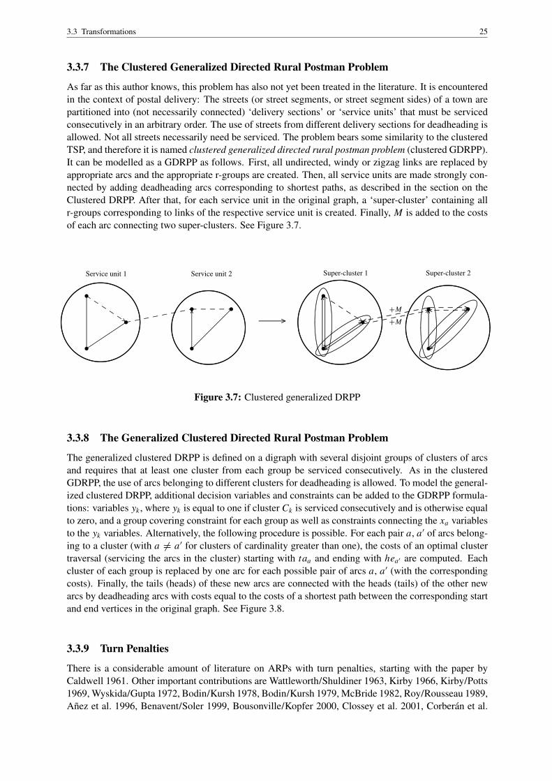
3.3 Transformations 25
3.3.7 The Clustered Generalized Directed Rural Postman Problem
As far as this author knows, this problem has also not yet been treated in the literature. It is encounteredin the context of postal delivery: The streets (or street segments, or street segment sides) of a town arepartitioned into (not necessarily connected) ‘delivery sections’ or ‘service units’ that must be servicedconsecutively in an arbitrary order. The use of streets from different delivery sections for deadheading isallowed. Not all streets necessarily need be serviced. The problem bears some similarity to the clusteredTSP, and therefore it is named clustered generalized directed rural postman problem (clustered GDRPP).It can be modelled as a GDRPP as follows. First, all undirected, windy or zigzag links are replaced byappropriate arcs and the appropriate r-groups are created. Then, all service units are made strongly con-nected by adding deadheading arcs corresponding to shortest paths, as described in the section on theClustered DRPP. After that, for each service unit in the original graph, a ‘super-cluster’ containing allr-groups corresponding to links of the respective service unit is created. Finally, M is added to the costsof each arc connecting two super-clusters. See Figure 3.7.
s
ss s
ss
........
........
........
........
........
........
........
........
........
........
........
........
........
........
........
........
........
.......
.................................................................................................................................
............. ............. ............. ............. ............. ........ ........ ............. ............. ............. ............. ............. ............. ............. .......
........
........
........
........
........
........
........
........
........
........
........
........
.......................
.................................................................................................................................................................... ............. ............. ............. .......
Service unit 1
pppppppppppppppppppppppppppppppppppppppppppppppppppppppppppppppppppppppppppppppppppppppppppppppppppppppppppppppppppppppppppppppppppppp
ppppppppppppppppppppppppppppppppppppppppppppppppppppppppppppppppppppppppppppppppppppppppppppppppppppppppppppppppppppppppppppppppppppppppppppppppppppppppppppppppppppppppppppppppppppppppppppppppppppppppppppppppppppppppppppppppppppppppppppppppppppppppppppppppppppppppppppppppppppppppppppppppppppppppppppppppppppppppppppppppppppppppppppppppppppppppppppppppppppppppppppppppppppppppppppppppppppppppppppppppppppppppppppppppppppppppppppppppppppppppppppppppppppppppppppppppppppppppppppppppppppppppppppppppppppppppppppppppppppppppppppppppppppppppp
Service unit 2
pppppppppppppppppppppppppppppppppppppppppppppppppppppppppppppppppppppppppppppppppppppppppppppppppppppppppppppppppppppppppppppppppppppppppppppppppppppppppppppppppppppppppppppppppppppppppppppppppppppppppppppppppppppppppppppppppppppppppppppppppppppppppppppppppppppppppppppppppppppppppppppppppppppppppppppppppppppppppppppppppppppppppppppppppppppppppppppppppppppppppppppppppppppppppppppppppppppppppppppppppppppppppppppppppppppppppppppppppppppppppppppppppppppppppppppppppppppppppppppppppppppppppppppppppppppppppppppppppppppppppppppppppppppppppppppppppppppppppppppppppppppppppppppppppppppppppppppppppppppppppppppppppppppppppppppppppp
.................................................................................... ............
s
ss s
ss
..........
..........
..........
..........
..........
..........
..........
..........
..........
..........
..........
..........
..........
..................... ........................................................................................................................................................................................
................................
................................
....................................... .............................................................................................................................................
............. ............. ............. ............. ............. ........ ........+M ............................................................................................................ +M............. ............. ............. ............. ............. ............. ............. ......... ........
..........
..........
..........
..........
..........
..........
..........
..........
..........
..........
...................
..........................
..........................
..........................
..........................
..........................
............................. ..................................................................................................................................................................
.................................................................................. ............. ............. ............. .......... ........
Super-cluster 1
pppppppppppppppppppppppppppppppppppppppppppppppppppppppppppppppppppppppppppppppppppppppppppppppppppppppppppppppppppppppppppppp
ppppppppppppppppppppppppppppppppppppppppppppppppppppppppppppppppppppppppppppppppppppppppppppppppppppppppppppppppppppppppppppppppppppppppppppppppppppppppppppppppppppppppppppppppppppppppppppppppppppppppppppppppppppppppppppppppppppppppppppppppppppppppppppppppppppppppppppppppppppppppppppppppppppppppppppppppppppppppppppppppppppppppppppppppppppppppppppppppppppppppppppppppppppppppppppppppppppppppppppppppppppppppppppppppppppppppppppppppppppppppppppppppppppppppppppppppppppppppppppppppppppppppppppppppppppppppppppppppppppppppppppppppppppppppppppppppppppppppppppppppppppppppppppppppp
ppppppppppppp
Super-cluster 2
pppppppppppppppppppppppppppppppppppppppppppppppppppppppppppppppppppppppppppppppppppppppppppppppppppppppppppppppppppppppppppppp
ppppppppppppppppppppppppppppppppppppppppppppppppppppppppppppppppppppppppppppppppppppppppppppppppppppppppppppppppppppppppppppppppppppppppppppppppppppppppppppppppppppppppppppppppppppppppppppppppppppppppppppppppppppppppppppppppppppppppppppppppppppppppppppppppppppppppppppppppppppppppppppppppppppppppppppppppppppppppppppppppppppppppppppppppppppppppppppppppppppppppppppppppppppppppppppppppppppppppppppppppppppppppppppppppppppppppppppppppppppppppppppppppppppppppppppppppppppppppppppppppppppppppppppppppppppppppppppppppppppppppppppppppppppppppppppppppppppppppppppppppppppppppppppppppp
ppppppppppppp............................................................................................................................................................................................................................................................................................
.................................................................................................................
..............................................................
...................................
...............................
...........................
...................................................................................................................................................................................................................................
...........................................................................................................................................................................................................................................................................
....................................................................................................
....................................................
...............................
............................
..........................
........................
.........................................................................................................................................................................................................................................................................................................
Figure 3.7: Clustered generalized DRPP
3.3.8 The Generalized Clustered Directed Rural Postman Problem
The generalized clustered DRPP is defined on a digraph with several disjoint groups of clusters of arcsand requires that at least one cluster from each group be serviced consecutively. As in the clusteredGDRPP, the use of arcs belonging to different clusters for deadheading is allowed. To model the general-ized clustered DRPP, additional decision variables and constraints can be added to the GDRPP formula-tions: variables yk , where yk is equal to one if cluster Ck is serviced consecutively and is otherwise equalto zero, and a group covering constraint for each group as well as constraints connecting the xa variablesto the yk variables. Alternatively, the following procedure is possible. For each pair a, a′ of arcs belong-ing to a cluster (with a 6= a′ for clusters of cardinality greater than one), the costs of an optimal clustertraversal (servicing the arcs in the cluster) starting with taa and ending with hea′ are computed. Eachcluster of each group is replaced by one arc for each possible pair of arcs a, a′ (with the correspondingcosts). Finally, the tails (heads) of these new arcs are connected with the heads (tails) of the other newarcs by deadheading arcs with costs equal to the costs of a shortest path between the corresponding startand end vertices in the original graph. See Figure 3.8.
3.3.9 Turn Penalties
There is a considerable amount of literature on ARPs with turn penalties, starting with the paper byCaldwell 1961. Other important contributions are Wattleworth/Shuldiner 1963, Kirby 1966, Kirby/Potts1969, Wyskida/Gupta 1972, Bodin/Kursh 1978, Bodin/Kursh 1979, McBride 1982, Roy/Rousseau 1989,Anez et al. 1996, Benavent/Soler 1999, Bousonville/Kopfer 2000, Clossey et al. 2001, Corberan et al.

3.3 Transformations 26
r-Group 1: c1, c3r-Group 2: c2
ss s
ss
ss
ac1........................
................................................
...................................................
bc2
.................................................................................................................................... ........
cc1
...........................................................................................d .......................................................................................................................................................................
e c2
...........................................................................................
fc3.........................................................................................................................................................
g c3
................................................................................................................
h
.............
.............
.............
.............................
.................................................................................... ............
abc.................
..................................
.............................................
cdea.................
..................................
.............................................
f hg.................
..................................
.............................................
g f.................
..................................
.............................................
eab.................
..................................
.............................................
bcde.................
..................................
.............................................
........................................................................................................................
0.............
..........................
..........................
..........................
..........................
..........................
.............................
cc + cd + ce
........................................................................................................................................................................................................................................................................................................................................................
........................................
..............................................................................................................................................
..........................
...................................
..........................................................
...............................................................................................................................................................................................................................................................................................................r-Group 1
.....................................................................................................................................................................................................................................
..............................................................................................
...........................
....................................................
........................................................................................................................................................................................r-Group 2
Figure 3.8: Generalized clustered DRPP
2002, Winter 2002, Arkin et al. 2005. Some authors develop solution algorithms working directly on thegraphs with turn penalties, others use transformations into arc or vertex routing problems without turnpenalties. A detailed review would go beyond the scope of this paper. In the following, two formulationsfor ARPs with turn penalties and the three basic possibilities of transformations into graphs without turnpenalties are presented.
This author is not aware of any publications considering direct exact approaches for ARPs with turnpenalties. The following two formulations are the first ones to use the concept of turn variables.
A possible formulation for the windy rural postman problem with turn penalties (WRPPTP) on a graphGT P = (V, L , T ) is as follows:
(WRPPTP1): ∑l∈L
(→cl→xl +
←cl←xl)+
∑t∈T
pet yt→ min subject to (3.11a)
→xl +←xl = 1 ∀ l ∈ L R (3.11b)∑
{l∈L:hel=i}
(→xl −
←xl)+∑
{l∈L:tal=i}
(←xl −
→xl) = 0 ∀ i ∈ V (3.11c)
∑{l∈L:tal∈ ·∪q∈S V CC
q 63hel }
→xl +∑
{l∈L:tal 6∈ ·∪q∈S V CCq 3hel }
←xl = 1 ∀ ∅ 6= S $ {1, . . . , pC}, |S| 5⌊ pC
2
⌋(3.11d)
→xl −∑
{t∈T :ilt=l,tvt=hel }
yt = 0 ∀ l ∈ L (3.11e)
→xl −∑
{t∈T :tvt=tal ,olt=l}
yt = 0 ∀ l ∈ L (3.11f)
←xl −∑
{t∈T :ilt=l,tvt=tal }
yt = 0 ∀ l ∈ L (3.11g)
←xl −∑
{t∈T :tvt=hel ,olt=l}
yt = 0 ∀ l ∈ L (3.11h)
→xl ∈ Z0+∀ l ∈ L (3.11i)
←xl ∈ Z0+∀ l ∈ L (3.11j)
yt ∈ Z0+∀ t ∈ T (3.11k)

3.3 Transformations 27
→xl (←xl) are link variables denoting the number of times link l ∈ L is traversed from tail to head (from headto tail). yt are turn variables denoting the number of times turn t is performed. The objective functionstrives to minimize the sum of link traversal costs and turn penalties.
Constraints (3.11b) guarantee covering of the required links. (3.11c) ensure flow conservation. (3.11d)ensure that a link between any subset of the pC required components and the complement of this subsetis used. It would not be sufficient to require this for every single required component, because thensubtours would be possible. (3.11e)–(3.11h) perform the coupling between the two types of variable. Ifa link is traversed in a certain direction, there must be a turn using this link as inlink and a turn using thislink as outlink, and these turns must traverse the link in the right direction.
Are subtour elimination constraints for the turns needed, too? Consider the so-called hourglass graphdepicted in Figure 3.9 (a). If all six depicted arcs are required, there is exactly one closed trail constitut-ing a postman tour. If there are no turn penalties and only arc variables are used, no subtours arise. Withturn penalties and turn variables, though, it is also possible to traverse all six arcs when the indicatedturns are performed, but this leads to two subtours.
s...................................................................................................................................................................
s.................................................................................................................................................................................................................................s.......................................................................................................................................................... ...................
......................
......................
......................
......................
......................
......................
...................s................................................................................................................................................................................................................................. s...................................................................................................................................................................
...................................
..........................................................................
.............................................................................................................
Figure 3.9: Hourglass graph
Constraints that avoid such subtours are∑{t∈T :ilt∈L(S),olt 6∈L(S)}
yt = 1 ∀ S $ V, L R(S) 6= ∅ (3.12)
(3.12) require that, for each proper subset S of the vertex set V for which a required link exists whosehead and tail vertices are elements of S, there must be a turn leaving S. In conjunction with flow con-servation constraints, (3.12) also ensure that, for each such S, there is a turn entering S, too. For subsetsof V with only one vertex, the constraints coupling the arc and the turn variables make sure that there isalways a turn leaving the respective subset.
However, consider the inverse hourglass graph in Figure 3.10. If all arcs are required, performing theindicated turns fulfils constraints (3.12), but again, there are two subtours.
s......................................................................................................................................................................................................................................................................................................................................................................................................................................................................
s...........
......................
......................
......................
......................
......................
......................
.................
................................................................................................................................................................s................................................................................
......................
......................
.................................
s.............................................................................................................................................................
.......................
..................
..................
.....................
..................................................................
...............
.................................................................................
.................................................................................
.................................................................................
Figure 3.10: Inverse hourglass graph

3.3 Transformations 28
To prevent such subtours, the following constraints can be used:∑t ′∈T ′
yt ′ = 1⇒∑
{t∈T :t 6∈T ′,∃t∈T ′ with olt=ilt ,tvt 6=tvt }
yt = 1 ∀ ∅ 6= T ′ $ T, |T ′| 5⌊|T |2
⌋(3.13)
(3.13) state that for each non-empty proper subset T ′ of the set T of turns containing not more than halfof all turns, the following must hold: If a turn t ′ ∈ T ′ is performed, another turn t not belonging to T ′
must be performed, and there must be a turn t ∈ T ′ whose outlink is the inlink of t , and whose turnvertexis not the turnvertex of t . Thus, constraints (3.13) must be added to (3.11). Constraints (3.11d) are thenredundant.
With constraints (3.13), a formulation using only turn variables can be stated as follows:
(WRPPTP2): ∑t∈T
(cilt + pet)yt→ min subject to (3.14a)
∑{t∈T :ilt=l}
yt = 1 ∀ l ∈ L R (3.14b)
∑{t∈T :ilt=l,tvt=hel }
yt −∑
{t∈T :olt=l,tvt=tal }
yt = 0 ∀ l ∈ L (3.14c)
∑{t∈T :ilt=l,tvt=tal }
yt −∑
{t∈T :olt=l,tvt=hel }
yt = 0 ∀ l ∈ L (3.14d)
∑t ′∈T ′
yt ′ = 1⇒∑
{t∈T :t 6∈T ′,∃t∈T ′ with olt=ilt ,tvt 6=tvt }
yt = 1 ∀ ∅ 6= T ′ $ T, |T ′| 5⌊|T |2
⌋(3.14e)
yt ∈ Z0+∀ t ∈ T (3.14f)
cilt in the objective function indicates the costs of traversal of the inlink of t in the direction in which ilt
is traversed in t . The meaning of the constraints should be clear from the preceding explanations.
To transform a graph GT P with turn penalties into a graph G without, there are three basic possibilities:
(i) A graph G is created which contains one arc for each possible direction of traversal of each linkof GT P . These arcs form the set S. Then, additional non-r-group arcs from the head of each arca ∈ S to the tail of each other arc a′ ∈ S are inserted if and only if the corresponding links areincident or identical in GT P , i.e., if and only if there is a turn in GT P with inlink equal to thelink corresponding to a, outlink equal to the link corresponding to a′, and finite turn penalty. Thecosts of these additional arcs are set to the corresponding turn penalty. An example (adapted fromGrunert/Irnich 2005b, p. 615) is given in Figure 3.11. As can be seen from the figure, an equivalenttransformation is to create a digraph D with one vertex for each possible direction of traversal ofeach link of GT P and one arc for each turn in GT P . The costs of an arc a in D must then includethe corresponding costs of traversal of the link in GT P corresponding to hea in D.This transformation is henceforth referred to as no sfw transformation.
(ii) A graph G is created which contains one r-group arc for each possible direction of traversal ofeach required link in GT P , and additional arcs leading from the head of each original r-group arca to the tail of each original r-group arc a′ are inserted. The costs of these additional arcs are set tothe costs of the shortest feasible walk from taa via a to hea′ via a′ minus ca minus ca′ . (This takesinto account the turn penalties.) The first turn penalty of the shortest feasible walk must not besubtracted. To compute such feasible walks, a slightly modified version of the Dijkstra algorithmcan be used, see Benavent/Soler 1999.This transformation is henceforth referred to as sfw transformation.

3.3 Transformations 29
(iii) A graph G is created which contains one vertex for each possible direction of traversal of each linkin GT P and one arc for each turn. The tail (head) of an arc in G is the vertex corresponding to theinlink (outlink) of the turn corresponding to the arc (see Figure 4.5 on page 79). Essentially, theformulation (3.14) on GT P is a formulation on G where the yt are arc variables. The presumablyfirst paper on routing problems with turn penalties (Caldwell 1961) was already proposing such atransformation, and Anez et al. 1996 call the resulting graph G the dual graph of GT P .
s
s
s
s
s
s
e2
........
........
........
........
........
........
........
........
........
........
........
........
........
........
........
........
........
.......
e1
........
........
........
........
........
........
........
........
........
........
........
........
........
........
........
........
........
.......
e3...............................................................................................................................................
e4
........
........
........
........
........
........
........
........
........
........
........
........
........
........
........
........
........
.......
a2.........................................................................................................................................................
a1.........................................................................................................................................................
a3
......................................................................................................................................................... .................................................................................... ............
s
s
s
s
s
s
s
s
s
ss
s
s
ss
s
s
s
s
s
s
s
→e2
........
........
........
........
........
........
........
........
........
........
........
........
........
........
........
........
........
.................
→e1
........
........
........
........
........
........
........
........
........
........
........
........
........
........
........
........
........
.................
←e2
.........................................................................................................................................................
←e1
.........................................................................................................................................................
a2.........................................................................................................................................................
→e3.........................................................................................................................................................
a1.........................................................................................................................................................
←e3 .........................................................................................................................................................
→e4
........
........
........
........
........
........
........
........
........
........
........
........
........
........
........
........
........
.................
←e4
.........................................................................................................................................................
a3
.........................................................................................................................................................
........
.....
........
.....
........
.....
........
.....
........
.....
........
....................
............. ............. .......................................................
..........................
..........................
.............................
............. ............. .......................................... ............. ............. ............. ............. .............................
.......................................................
....................................................... .............
.............
.............
.............
.............
............................
............. ............. ............. ........ ........
............. ............. ............. ........ ........
.......................................................
..........................
..........................
..........................
.............................
........
.....
........
.....
........
.....
.......................................................................
..........................
.............................
..........................
..........................
..........................
............. ........ ........
............. ............. ............. ............. ............. ..................... ........
..........................
..............................
..........................
..........................
..........................
.............................
............. ............. .............................
.......................................................
.............
.............
.............
.............
.............
............................
Figure 3.11: Transformation of a graph with turn penalties into one without
3.3.10 Zigzag Service
The issue of zigzag service also arises in the context of postal delivery. Imagine a postman who mustdeliver mail in a street segment between two road junctions. There are houses on both sides of the streetsegment. If there is not too much traffic in the segment, the postman has several possibilities for servicingit: He may service one side at a time (and not necessarily both sides contiguously), which means that hemust traverse the street segment at least twice, and he may service both sides simultaneously (in ‘zigzagmode’), which means that he must traverse the street segment only once. See Figure 3.12.
...................................................................................................................................................................................
...................................................................................................................................................................................
........
........
........
........
........
........
........
........
..................................................................................................................................................................................................................................................................................................................................................................................................................................................................................................................................................................................................
..................................................................................................................................................................................................................................................................................................................................................................................................................................................................................................................................................................................................................................................................
........
........
........
........
........
........
........
........
...................................................................................................................
...................................................................................................................................................................................
........
........
........
........
.....................................................................................................................................................................
........
........
........
........................................................................................... .....................................................................................................................................................................................................
........
........
........
...........................................................................................
........
........
........
........
.....................................................................................................................................................................
........
........
........
........................................................................................... ............................................................................................................................................................................................................................................
............................................................................................................................................................................................................................................................................................................................................................................................................................................................................................................................................................................................................................................................................................................................................................................................................................................................................................................................................................................................................................................................................ ........
........
........
........
............................................................................................................................................................................................................
........................................................................................................................................................................................................................................................................................................................
........................................................................................................................................................................................................................................................................................................................
........................................................................................................................................................................................................................................................................................................................
............................................................................
........
........
........
........
............................................................................................................................................................................................................
........................................................................................................................................................................................................................................................................................................................
........................................................................................................................................................................................................................................................................................................................
........................................................................................................................................................................................................................................................................................................................
........................................................................................................................................................................................................................................................................................................................................................................
............................................................................ ........
........
........
........
............................................................................................................................................................................................................
............................................................................................................................................................................................................................................................................................................................................................................................................................................................................................................................................................................................................................................................................................................................................................................................................................ ........
........
........
........
............................................................................................................................................................................................................
............................................................................
....................................................................................................................................................................................................................................................................................................................................................................................................................................................... ............................................
....................................................................................................................................................................................................................................................................................................................................................................................................................................................... ............................................pppppppppppppppppppppppppppppppppppppppppppppppppppppppppppppppppppppppppppppppppppppppppppppppppppppppppppppppppppppppppppppppppppppppppppppppppppppppppppppppppppppppppppppppppppppppppppppppppppppppppppppppppppppppppppppppppppppppppppppppppppppppppppppppppppppppppppppppppppppppppppppppppppppppppppppppppppp
pppppppppppppppppppppppppppppppppppppppppppppppppppppppppppppppppppppppppppppppppppppppppppppppppppppppppppppppppppppppppppppppppppppppppppppppppppppppppppppppppppppppppppppppppppppppppppppppppppppppppppppppppppppppppppppppppppppppppppppp pppppppppppp
Crossing A Crossing B
Street segment side 2
Street segment side 1
Figure 3.12: Street with zigzag service option
Thus, zigzag service of a required link means that it can be serviced by traversing it once in each direc-tion, by traversing it twice from tail to head, by traversing it twice from head to tail, or by traversing itonce in any direction in ‘zigzag mode’. Figure 3.13 shows how this can be modelled by two non-disjointr-groups. For a potential zigzag service street segment, two vertices, eight arcs, and two r-groups are

3.3 Transformations 30
introduced. There are two non-r-group deadheading arcs, one for each direction, two antiparallel r-grouparcs for each street segment side, and two antiparallel r-group arcs for zigzagging. To service the streetsegment, the postman must either use one of the zigzag arcs or two ‘street segment side arcs’, one foreach street segment side. Grouping the arcs in two non-disjoint r-groups, one for each street segmentside, such that the two zigzag arcs belong to the intersection of the r-groups, yields the desired result.
A B....................................... ............. ............. ............. ............. ............. ............. ............. ............. ............. ............. ..........................
....................................
..........................
.............................................................................................................................................................................................................
...................................................................................................................................................................................................................................................................................................................................................................................
....................................................................................................................................................................................................................................................................................................................
...................................................................................................................................................................................................................................................................................................
................................. .................................................................................................................................................................................................................................................................................................................
....................
...............................
pppppppppppppppppppppppppppppppppppppppppppppppppppppppppppppppppppppppppppppppppppppppppppppppppppppppppppppppppppppppppppppppppppppppppppppppppppppppppppppppppppppppppppppppppppppppppppppppppppppppppppppppppppppppppppppppppppppppppppppppppppppppppppppppppppppppppppppppppppppppppppppppppppppppppp pppppppp pppppppppppppppppppppppppppppppppppppppppppppppppppppppppppppppppppppppppppppppppppppppppppppppppppppppppppppppppppppppppppppppppppppppppppppppppppppppppppppppppppppppppppppppppppppppppppppppppppppppppppppppppppppppppppppppppppppppppppppppppppppppppppppppppppppppppppppppppppppppppppppppppppppppppppppppppp r-Groups..................................................................................................... ............
.......................................................................................................................................................................
........................................................................................................................................................... ............
pppppppppppppppppppppppppppppppppppppppppppppppppppppppppppppppppppppppppppppppppppppppppppppppppppppppppppppppppppppppppppppppppppppppppppppppppppppppppppppppppppppppppppppppppppppppppppppppppppppppppppppppppppppppppppppppppppppppppppppppppppppppppppppppppppppppppppppppppppppppppppppppppppppppppppppppppppppppppppppppppp pppppppppppp.......................................................................................................................................................................
........................................................................................................................................................... ............
..........................................................................................................................................................................................................................................................................................................................................................................................................................................................
...................................
.................................................................
...........................
............................................
.............................................................................
Deadheading arc
Zigzag arcs
Street segment side 1
Street segment side 2
Figure 3.13: Modelling of zigzag service in a GDRPP
An alternative approach for considering zigzag service is proposed by Irnich 2005.
3.3.11 Different Costs for Servicing and Deadheading in Different Directions
An extension recently considered by Lacomme et al. 2004 is the possibility of two different costs perlink for traversal with and without servicing. For windy graphs, this must be generalized to four differentcosts, depending on the direction of traversal and on whether the link is being serviced or not. This,too, can be modelled within a GDRPP, by introducing two service and two deadheading antiparallel arcsfor each such windy link, where the two service arcs form one r-group. Note that, for uncapacitatedproblems, or, to be precise, for problems without resource constraints, on a windy graph G = (V, L), itis necessary to distinguish between costs for traversal with and without service if and only if the condition
→c dl −
→c sl =
←c dl −
←c sl (3.15)
is violated, where →c dl and ←c d
l are the costs for deadheading through a link l ∈ L from tail to head andfrom head to tail respectively, and where →c s
l and ←c sl are the costs for servicing l from tail to head and from
head to tail. This can be seen as follows. The overall cost contribution of a link l to a postman tour is→c d
l→x d
l +→c s
l→x s
l +←c d
l←x d
l +←c s
l←x s
l , (3.16)
where →x dl is the number of deadheading traversals of l from tail to head, and where →x s
l , ←x dl , and ←x s
l aredefined analogously. For fixed values of →x d
l +→x s
l and ←x dl +
←x sl , assume w.l.o.g. →x s
l = 1 and ←x sl = 0. If
this is to be changed to →x sl = 0 and ←x s
l = 1, (3.16) changes by →c dl −
→c sl +
←c sl −
←c dl , which is equal to zero
if →c dl =
→c sl and ←c d
l =←c s
l . If the costs of traversal and of servicing are no longer the same, (3.16) remainsunchanged if and only if (3.15) holds.
3.3.12 Complexity Results
After the detailed description of the transformations, some remarks on the difficulty of the consideredproblems are appropriate, as the interest of transformations from one problem type into another is, in gen-eral, limited to N P-hard problems. With the exception of the undirected and directed CPP, for whichEdmonds/Johnson 1973 give polynomial algorithms, all considered arc routing problems are N P-hard(Dror 2000a). All considered vertex routing and rural postman problems are even N P-hard in thestrong sense. The former is shown in Johnson/Papadimitriou 1985, the latter is easily seen by reducingthe STSP to the undirected RPP (URPP): A graph of an STSP instance is polynomially transformed intoa graph of a URPP instance by creating a duplicate of each vertex and connecting each original vertexwith its duplicate by an edge with costs of zero. The additional edges are required; all original edgesare non-required. Moreover, Corberan et al. 2002 prove that postman problems with turn penalties areN P-hard in the strong sense. Consequently, the GDRPP itself is strongly N P-hard as well.

3.4 Solution Approaches 31
3.4 Solution Approaches
The transformations presented in the previous section show the genericity and flexibility of the GDRPPmodel, thus suggesting that it is worthwhile to develop good algorithms for it. However, as the GDRPPis a hard problem, heuristics are needed to be able to solve large real-world instances in reasonable time.So, in this section, exact as well as heuristic algorithms are presented.
3.4.1 A Labelling Algorithm for the GDRPP
Noon/Bean 1991 mention several early papers (which were not accessible to this author) that tackle theTSP and the GTSP by dynamic programming algorithms ‘in which a state is defined by the sets alreadyvisited’ (ib., p. 624). The ideas of these authors can be adapted to construct a labelling algorithm for theGDRPP.
GDRPP-Exact-Labelling (GDRPP-EL):Given: a digraph D = (V, A) defining a GDRPP instance.Select an r-group of minimal cardinality. Let this r-group be q1 (w.l.o.g.).For each arc acurr in q1:
Modify D by adding an artificial destination vertex d ′ and an arc from taacurr to d ′ with costs ofcacurr .Solve an SPPRC on the modified digraph by a labelling algorithm. To this end, introduce a car-dinally scaled, unconstrained resource r cost measuring the costs and one nominally scaled binaryresource rq , indicating whether r-group q must still be covered, for each r-group, except for q1 andall other r-groups covered by acurr . Set the resource windows for all resources at all vertices to[0,+∞[, except for d ′, where all resource windows for r-group covering are set to [0, 0]. Use thefollowing resource variables and resource extension functions: For r cost , use a resource variableσ cost
i at vertex i and the REF f rcostwith f rcost
a (σ costtaa
) = σ costtaa+ ca . For r-group q, use a resource
variable σqi at vertex i and the REF f rq
with f rq
a (σqtaa ) = max{0, σ
qtaa − δq
a }, where δqa is equal
to one if and only if a ∈ Aq and is otherwise equal to zero. Start with a first label l1, resident atheacurr , set l1’s cost resource variable to zero and all its other resource variables to one (true). Seeka shortest walk from heacurr to d ′ using the following dominance procedure: Label l dominates la-bel l ′ if and only if l has covered all r-groups l ′ has covered and has not accumulated greater coststhan l ′. If l has covered an r-group which l ′ has not and vice versa, the two labels are incomparable.(To avoid two labels dominating each other, the labels can be numbered and the rule can be addedthat, in case of a tie, the label with the smaller number dominates the other label.)
The solution of the SPPRC with the smallest objective function value yields an optimal solution to theGDRPP instance, when the arc d ′ is replaced by the corresponding arc a.
It is not sufficient to compute a shortest path from o := hea to d := taa for each arc a from r-groupq1, because, as can be seen in Figure 3.14, there may be instances where it is necessary to visit d beforehaving covered all other r-groups. Therefore, the artificial destination vertex d ′ is introduced.
ss
sd
o
.........................................................................................................................................
q1
......................................................................................................................
q2
..........................
.............................. ........ .....................................................................................................
q3
Figure 3.14: GDRPP instance showing necessity of artificial vertex

3.4 Solution Approaches 32
Note that it is not a good idea to introduce an artificial source and sink vertex, to connect the source withthe tails of the r-group arcs, and to connect all heads, i.e., all vertices, with the sink. This is becausea postman tour is sought, not an open walk. Hence, a label would need to store the first ‘real’ vertexreached, and at the last vertex before the artificial sink, the shortest path distance back to this first realvertex would have to be added to the current costs. This is not a real difficulty; but what does make thisapproach unfavourable is the fact that the number of labels would increase considerably; in principle, anSPPRC for each tail of each r-group arc would be solved.
For computational purposes, a resource counting the number of already covered r-groups can be added,similar to the proposal of Feillet et al. 2004.
If more than one SPPRC must be solved, the optimal objective function value over all previously solvedSPPRCs can be used as a bound in each SPPRC. To use the bound, the value of the cost resource of alabel is checked when it is selected for extension. If this value is not strictly less than the bound, thelabel can be discarded. If the labels to be extended are selected from the set of unprocessed labels innon-decreasing order of their costs, the current SPPRC can be terminated/bounded altogether as soon asa label is selected for extension whose cost resource value exceeds the bound. To implement this strategyin the r c shortest path functions, a specialized visitor type can be used which accordingly definesthe function for the event point when a label is selected for extension.
Similar to the GTSP, the number of r-groups strongly influences the difficulty of an instance. Therefore,an alternative concerning the selection of the arcs for which an SPPRC is solved is to compute, for eacharc, the number of remaining r-groups in the corresponding SPPRC and to select the r-group q where themaximal number of remaining r-groups, taken over all arcs covering q , is minimal. Consider, for exam-ple, an instance with ten r-groups, one r-group with two arcs, each of them covering only this r-group,and one r-group with three arcs, each of them covering four r-groups. The alternatives are then to solvetwo SPPRCs with nine r-groups or three SPPRCs with six r-groups; the latter is clearly preferable. Ofcourse, this argument is of no use when the r-groups are disjoint. For graphs modelling road networks,not much is to be gained.
How can the dominance procedure be implemented? It is natural to store the information on which r-groups must still be covered in a container of Boolean variables. To decide whether a label/containerl dominates a label/container l ′, one possibility is to compare the two containers element by element.Another possibility is based on the following observation: If the number of already covered r-groupsis stored, the difference in the number of covered r-groups between l and l ′ can be computed. If thisdifference is negative, ‘l does not dominate l ′’ can be returned directly. Otherwise, this difference isupdated after each pairwise comparison of the ‘covered’ values of the two containers for one r-group. Ifl has already covered some r-group q and l ′ has not, the difference value is decreased by one. As soonas the updated difference value becomes negative, the procedure is stopped and ‘l does not dominatel ′’ is returned. A theoretical argument as to which procedure should be faster in the average case is asfollows. Consider two containers l, l ′ of size n of Boolean variables storing realizations of independentand identically distributed random variables taking on the values 0 and 1 with probability 1
2 . The expectedvalue of the number of bits set in each container is then n
2 . The simple dominance check can be stoppedat the first index i with l[i] < l ′[i]. The probability for this event is 1
4 , and therefore, on average, fourpairwise comparisons must be made. The probability of having to traverse both sequences until index nequals
1−n−2∑i=0
(34
)i 14.
With the second comparison strategy, the expected value of the difference in the number of covered r-groups is zero. This means that the comparison can be terminated at the first index i with l[i] < l ′[i],and also at the first index i ′ where it is the other way round, because then there must be an index i ′′ 6= i ′

3.4 Solution Approaches 33
with l[i ′′] < l ′[i ′′]. In both cases, l cannot dominate l ′. The probability that l[i] < l ′[i] or l[i] > l ′[i]is 1
2 , and therefore, on average, two pairwise comparisons must be made. The probability of having totraverse both sequences until index n equals
1−n−2∑i=0
(12
)i 12.
However, there is an additional overhead incurred by the more complex checking, as there are two ad-ditional operations for each index: updating of the difference value and checking it against zero. Theexpected number of elementary operations with the first strategy is 4 · 1 = 4, the expected number withthe second strategy is 2 · (1+1+1) = 6. Consequently, the second strategy does not seem advantageous.Computational experiments have indeed shown that, for the GDRPP, the more sophisticated check isoutperformed by the simpler pairwise comparison.
The approach of solving the GDRPP by a labelling algorithm has several advantages:
• The usual case in the literature for routing problems is to assume a non-negative link cost function,so, the SPPRC for the GDRPP need be solved only on a digraph without negative cycles. Asexplained in Chapter 2, SPPRCs on digraphs with negative cycles are much more difficult to solve.Strictly speaking, on digraphs with negative cycles, no minimal cost postman tour exists. To obtaina tour covering all r-groups, the number of traversals of each arc must be limited. This requiresadditional resources, and these resources increase the number of possible labels and the number oflabel incompatibilities.
• Solving the GDRPP by transforming it to a TSP requires adding deadheading arcs correspondingto shortest paths. When solving it as an SPPRC, this is not necessary. Instead, it is possible tooperate directly on the original digraph. There is no need for preprocessing (other than addingthe artificial destination vertex). More importantly, TSP algorithms always operate on completegraphs, whereas the labelling algorithm benefits if the original graph is sparse (which is the casefor graphs representing road networks).
• It is possible to handle non-disjoint r-groups without any modification.
• Some of the transformations described above require the introduction of degenerate cost structures(through the M constants). This might lead to numerical problems for LP-based methods, whereassuch cost structures are not critical for labelling algorithms.
The drawback of this approach is that, for dense graphs (e.g., for transformed TSP instances), and, ofcourse, for graphs with many r-groups, there may be very many incompatible labels. In fact, a worst-caseanalysis of the space and time complexity of GDRPP-EL on a digraph D = (V, A) yields the followingresults: The number of SPPRCs to be solved is at most |A|. In each SPPRC, at each vertex, there can be|A|(|A| − 1)2pA different undominated labels. This is because each time a vertex is reached via the samearc, there will be at least one additional covered r-group, or else the resulting label will be dominated.With each new label, a dominance check is performed by comparing it with every other label resident atthe same vertex. Hence, the space complexity of the labelling algorithm is O(|V ||A|22pA), and the timecomplexity is O(|A|522pA), which is exponential—but this was to be expected for a strongly N P-hardproblem.
Also, the clustered ATSP can be solved via an SPPRC algorithm. The principle is as follows. A resourceis introduced for each cluster C . At each vertex, the resource windows corresponding to a cluster thevertex does not cover are set to [0, 0], and the resource windows corresponding to a cluster the vertexdoes cover are set to [0, |C |], where |C | is the number of vertices belonging to C . The algorithm isstarted with a label l at a vertex from an arbitrary cluster C1 containing at least two vertices, and all ofl’s resource variables are set to M , except for the resource variable for C1, which is set to one. When a

3.4 Solution Approaches 34
vertex of cluster Ci is reached, the variable for Ci is increased by 1, and the variables for all other clustersare set to M . After having reached all vertices in Ci , the variables for all other clusters not yet coveredare set to zero.
3.4.2 Heuristics
It is also possible to use the labelling algorithm to solve the GDRPP heuristically. To this end, thecheck of the covered r-groups in the dominance procedure is omitted. A label l dominates a label l ′
already if l has either lower costs and covered at least as many r-groups as l ′ or l has the same costsand covered more r-groups than l ′. This simplified dominance procedure makes the algorithm faster byseveral orders of magnitude: It is then of polynomial complexity. However, the simplified algorithm isno longer exact, because it is then possible that a path is dominated by another path although both coverdifferent r-groups. The dominated path could possibly have covered r-groups which the dominating pathstill has to cover, and it could have done so in a much more efficient manner, and the dominating pathcould have covered r-groups which the dominated path still has to visit in a very inefficient manner.Consider, for example, Figure 3.15 (a). The arc a1 from h to i is the only arc covering r-group q1.Hence, h is connected with the artificial destination vertex d ′, and the algorithm seeks a shortest pathfrom i to d ′ covering all r-groups except for q1. If the costs of a3 are higher than the costs of a2, thelabel corresponding to the path (i, a3, j) is dominated by the label corresponding to the path (i, a2, j).However, in order to cover r-group q3, the algorithm has to loop once around the digraph to yield a la-bel corresponding to the path (i, a2, j, a4, k, a5, h, a1, i). The path (i, a2, j, a4, k, a5, h, a1, i, a3, j) willthen not be dominated, because it has covered more r-groups than any other path for which there is alabel at vertex j . The solution will be the path (i, a2, j, a4, k, a5, h, a1, i, a3, j, a4, k, a5, h, a′, d ′), al-though the evident optimal solution is (i, a3, j, a4, k, a5, h, a′, d ′). Moreover, the algorithm may evenfail altogether, i.e., may not return a feasible solution although one exists. This may occur when, at acertain vertex, each label that has covered a certain r-group is dominated by another label that has notcovered this r-group. The algorithm will then terminate without having created a label/path coveringall r-groups, and, hence, without having reached d ′. An example is provided in Figure 3.15 (b). Thelabels corresponding to the paths (o, a1, h, a3, i, a5, j) and (o, a1, h, a3, i, a4, o, a2, j), which cover q2,are dominated by the label corresponding to the path (o, a2, j, a6, k, a7, j), which covers q3, as all pathscover one r-group, but the third one is the shortest. On the other hand, the label corresponding to the path(o, a2, j, a6, k, a7, j, a6, k, a8, o), which also covers q3, is dominated by the path (o, a1, h, a3, i, a4, o)
for the same reason.
ss
s s sh i j k
d ′
a1 a2
a3 ca3 > ca2
a4
a5
a′q1 q2 q2
q3
q4
..........................
..........................
.............................
......................................................................................................................................................... ......................................................................................................................................................... ...................................................................................................................................................................................
.............................. ....................................................................................................................................................................................
...........................
................................
........................................
.............................................................
................................................................................................................................................................................................................................................................................................
(a) .............................................................................................................................................................................................................................................................................................
s s s ss
sh i j k
o
d ′
a1 a2
a3
a4
a5 a6
a7
a8
a′
q1
q2 q3
ca1 = ca3 = ca4 = ca5 = 10ca2 = ca6 = ca7 = 1
ca8 = 100
..........................................................................................................................................
..........................
..........................
...................................................................................................................................................................................... .................................................................................
............. ............. ............. ............. ............. ............................ ......................................................................................................................................................... ...................
....................................
....................................
....................................
....................................
....................................
..............................................
..........................
..........................
.............................
....................................
.................................................................
.............
......
(b)
Figure 3.15: GDRPP-HL (a) is a heuristic and (b) may fail
In addition to the heuristic labelling algorithm (henceforth called GDRPP-HL), the following genericconstructive heuristic is proposed. Contrary to GDRPP-HL, it guarantees to compute a feasible solutionfor any feasible instance.

3.4 Solution Approaches 35
GDRPP-Constructive (GDRPP-C):Given: a digraph defining a GDRPP instance.Compute the shortest paths from the head of each r-group arc to the tail of each r-group arc.Initiate the solution cycle with a trail consisting of one r-group arc which is a shortest one among allr-group arcs covering the highest number of r-groups.Mark all r-groups covered by this arc as covered.While not all r-groups are covered:
Select an arc a.Extend the current trail by adding (in the right sequence) the arcs on the shortest path from thehead of the last arc in the current trail to the tail of a and the arc a itself.Mark all previously uncovered r-groups covered by one of the newly added arcs as covered.
To obtain a cycle, extend the current trail by adding the arcs on the shortest path from the head of the lastarc added to the tail of the first arc added.
Two different criteria for the arc selection step are proposed:
GDRPP-Nearest-Neighbour (GDRPP-NN):Select an arc a covering the highest number of not yet covered r-groups among all closest r-group arcs.a is a closest one if the costs of the shortest path from the head of the last arc in the current trail to thetail of a plus ca are minimal over all r-group arcs covering a not yet covered r-group.
GDRPP-Best-Covering (GDRPP-BC):Select a closest arc a among all r-group arcs covering the highest number of not yet covered r-groups.
For disjoint r-groups, both heuristics yield the same solution (if both are coded in the same way withrespect to ordering, tie-breaking etc.).
The following two improvement heuristics are proposed:
GDRPP-Swap-Arcs (GDRPP-SA):Given: a cycle constituting a feasible GDRPP solution.For each r-group arc a:
Remove a at one of its most isolated positions. Remove here means that the arcs between the headof the preceding r-group arc and the tail of the succeeding r-group arc are replaced by the arcs ofa shortest path between these two vertices. A position of a is a most isolated one if the distancein the cycle from the head of the preceding r-group arc to the tail of the succeeding r-group arc ismaximal over all appearances of a in the cycle.For each r-group q that a covers:
If there is no other arc that covers q:Insert into the cycle, at a best possible position between two successive r-group arcsa1, a2, another arc a′ that covers q . Insert here means that all non-r-group arcs (if any)between a1 and a2 are replaced by the arcs of a shortest path from the head of a1 to thetail of a′ via a′ itself to the tail of a2. A best possible position is one leading to the lowestincrease in the costs of the cycle.
If the resulting cycle is shorter than the current best one, replace the current best one by the result-ing cycle.
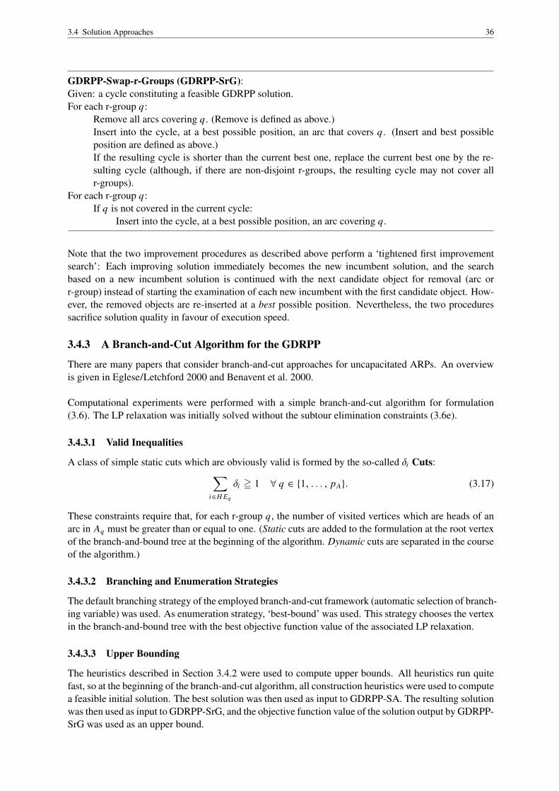
3.4 Solution Approaches 36
GDRPP-Swap-r-Groups (GDRPP-SrG):Given: a cycle constituting a feasible GDRPP solution.For each r-group q:
Remove all arcs covering q . (Remove is defined as above.)Insert into the cycle, at a best possible position, an arc that covers q . (Insert and best possibleposition are defined as above.)If the resulting cycle is shorter than the current best one, replace the current best one by the re-sulting cycle (although, if there are non-disjoint r-groups, the resulting cycle may not cover allr-groups).
For each r-group q:If q is not covered in the current cycle:
Insert into the cycle, at a best possible position, an arc covering q .
Note that the two improvement procedures as described above perform a ‘tightened first improvementsearch’: Each improving solution immediately becomes the new incumbent solution, and the searchbased on a new incumbent solution is continued with the next candidate object for removal (arc orr-group) instead of starting the examination of each new incumbent with the first candidate object. How-ever, the removed objects are re-inserted at a best possible position. Nevertheless, the two proceduressacrifice solution quality in favour of execution speed.
3.4.3 A Branch-and-Cut Algorithm for the GDRPP
There are many papers that consider branch-and-cut approaches for uncapacitated ARPs. An overviewis given in Eglese/Letchford 2000 and Benavent et al. 2000.
Computational experiments were performed with a simple branch-and-cut algorithm for formulation(3.6). The LP relaxation was initially solved without the subtour elimination constraints (3.6e).
3.4.3.1 Valid Inequalities
A class of simple static cuts which are obviously valid is formed by the so-called δi Cuts:∑i∈H Eq
δi = 1 ∀ q ∈ {1, . . . , pA}. (3.17)
These constraints require that, for each r-group q, the number of visited vertices which are heads of anarc in Aq must be greater than or equal to one. (Static cuts are added to the formulation at the root vertexof the branch-and-bound tree at the beginning of the algorithm. Dynamic cuts are separated in the courseof the algorithm.)
3.4.3.2 Branching and Enumeration Strategies
The default branching strategy of the employed branch-and-cut framework (automatic selection of branch-ing variable) was used. As enumeration strategy, ‘best-bound’ was used. This strategy chooses the vertexin the branch-and-bound tree with the best objective function value of the associated LP relaxation.
3.4.3.3 Upper Bounding
The heuristics described in Section 3.4.2 were used to compute upper bounds. All heuristics run quitefast, so at the beginning of the branch-and-cut algorithm, all construction heuristics were used to computea feasible initial solution. The best solution was then used as input to GDRPP-SA. The resulting solutionwas then used as input to GDRPP-SrG, and the objective function value of the solution output by GDRPP-SrG was used as an upper bound.
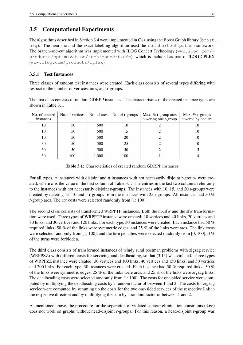
3.5 Computational Experiments 37
3.5 Computational Experiments
The algorithms described in Section 3.4 were implemented in C++ using the Boost Graph library (boost.-org). The heuristic and the exact labelling algorithm used the r c shortest paths framework.The branch-and-cut algorithm was implemented with ILOG Concert Technology (www.ilog.com/-products/optimization/tech/concert.cfm), which is included as part of ILOG CPLEX(www.ilog.com/products/cplex).
3.5.1 Test Instances
Three classes of random test instances were created. Each class consists of several types differing withrespect to the number of vertices, arcs, and r-groups.
The first class consists of random GDRPP instances. The characteristics of the created instance types areshown in Table 3.1.
No. of created No. of vertices No. of arcs No. of r-groups Max. % r-group arcs Max. % r-groupsinstances covering one r-group covered by one arc
10 50 500 10 2 1010 50 500 15 2 1010 50 500 20 2 1030 50 500 25 2 1030 50 500 50 2 530 100 1,000 100 1 4
Table 3.1: Characteristics of created random GDRPP instances
For all types, n instances with disjoint and n instances with not necessarily disjoint r-groups were cre-ated, where n is the value in the first column of Table 3.1. The entries in the last two columns refer onlyto the instances with not necessarily disjoint r-groups. The instances with 10, 15, and 20 r-groups werecreated by deleting 15, 10 and 5 r-groups from the instances with 25 r-groups. All instances had 50 %r-group arcs. The arc costs were selected randomly from [1; 100].
The second class consists of transformed WRPPTP instances. Both the no sfw and the sfw transforma-tion were used. Three types of WRPPTP instance were created: 10 vertices and 40 links, 20 vertices and80 links, and 30 vertices and 120 links. For each type, 30 instances were created. Each instance had 50 %required links. 50 % of the links were symmetric edges, and 25 % of the links were arcs. The link costswere selected randomly from [1; 100], and the turn penalties were selected randomly from [0; 100]. 3 %of the turns were forbidden.
The third class consists of transformed instances of windy rural postman problems with zigzag service(WRPPZZ) with different costs for servicing and deadheading, so that (3.15) was violated. Three typesof WRPPZZ instance were created: 30 vertices and 100 links, 40 vertices and 150 links, and 50 verticesand 200 links. For each type, 30 instances were created. Each instance had 50 % required links. 50 %of the links were symmetric edges, 25 % of the links were arcs, and 25 % of the links were zigzag links.The deadheading costs were selected randomly from [1; 100]. The costs for one-sided service were com-puted by multiplying the deadheading costs by a random factor of between 1 and 2. The costs for zigzagservice were computed by summing up the costs for the two one-sided services of the respective link inthe respective direction and by multiplying the sum by a random factor of between 1 and 2.
As mentioned above, the procedure for the separation of violated subtour elimination constraints (3.6e)does not work on graphs without head-disjoint r-groups. For this reason, a head-disjoint r-group was

3.5 Computational Experiments 38
added to all test instances without prior testing for whether an instance already contained such an r-group.
3.5.2 System Parameters
The system parameters used in the computational experiments are shown in the following table. AllCPLEX parameters not shown in the table were at their default values. The selection of the algorithmfor solving the LP relaxations was left to CPLEX. The maximum flow problems for the separation of thesubtour elimination constraints were solved with the Edmonds-Karp algorithm provided by the BGL.
Parameter Setting
CPU frequency 1 GHzMain memory 1 GBCPLEX version 9.1Concert Technology version 2.1Wall-clock time limit for branch-and-cut 3,900 secondsMin. violation of subtour eliminationconstraints to be considered violated 10−3
IloCplex::EpAGap 10−4
IloCplex::EpInt 10−4
IloCplex::CutLo −1075
IloCplex::EpGap 10−4
IloCplex::ObjDif 0IloCplex::RelObjDif 0IloCplex::CutUp 1075
Table 3.2: System parameters GDRPP
Due to the used operating system, all reported running times (in this chapter as well as in the chapterson the VRPTT and the TTRP) are wall-clock times and, hence, are subject to considerable variations.However, as a high number of instances was used for each instance class and type, and as all experimentswere performed on a ‘dedicated’ PC that was not used otherwise during the experiments, the variationsshould be quite balanced on average.
3.5.3 Computational Results
In the following tables, the random GDRPP instance types are denoted v a r s, where v indicates thenumber of vertices, a indicates the number of arcs, r indicates the number of r-groups, and s ∈ {y, n},where y means that the r-groups are disjoint, and n means that they are not necessarily disjoint. The trans-formed WRPPTP instances are denoted v a s, where v denotes the number of vertices in the WRPPTPinstances, a denotes the number of arcs in the WRPPTP instances, and s ∈ {no s f w, s f w} denotes thetype of transformation. The transformed WRPPZZ instances are denoted v a, where v and a denote thenumber of vertices and arcs respectively in the WRPPZZ instances. Here and in the following chapters,table entries of the form x / y / z denote the minimal, average, and maximal value respectively.
3.5.3.1 Results for the Exact Labelling Algorithm
The complexity analysis of the exact labelling algorithm in section 3.4.1 has shown that the algorithm’stime and space complexity are determined by the number of r-groups. As was to be expected from thisanalysis, GDRPP-EL was able to solve only the smallest instances, i.e., those with the smallest numberof r-groups. The following table shows how the running times of GDRPP-EL compare with those of the

3.5 Computational Experiments 39
branch-and-cut algorithm. The rows with the heading ‘Rank time’ indicate the rank of the respectiveprocedure in a ranking of running time over all procedures. For example, 1/2.3/4 means that for atleast one instance, no other procedure was faster; the average rank over all instances is 2.3, and for allinstances, the procedure was at least the fourth-fastest.
Branch-and-cut algorithmGDRPP-EL No cuts, no UB Cuts, no UB No cuts, UB Cuts, UB
50 500 10 nRunning time [s] 20 / 69 / 137 0 / 53 / 257 0 / 40 / 261 0 / 44 / 146 0 / 26 / 125Rank time 3 / 4.2 / 5 1 / 2.7 / 5 1 / 2.1 / 5 2 / 3.3 / 5 1 / 2.7 / 4
50 500 10 yRunning time [s] 20 / 47 / 89 0 / 32 / 260 0 / 19 / 130 0 / 38 / 263 0 / 23 / 188Rank time 1 / 4.5 / 5 1 / 2.5 / 4 1 / 2.1 / 4 1 / 3.0 / 5 1 / 2.5 / 4
50 500 15 nRunning time [s] 774 / 8,161 / 24,733 0 / 22 / 125 0 / 192 / 753 0 / 61 / 319 0 / 99 / 601Rank time 5 / 5.0 / 5 1 / 1.6 / 3 1 / 2.7 / 4 1 / 2.5 / 4 1 / 3.2 / 4
50 500 15 yRunning time [s] 1,326 / 10,231 / 20,254 0 / 6 / 22 0 / 10 / 29 0 / 6 / 15 0 / 10 / 29Rank time 5 / 5.0 / 5 1 / 2.0 / 4 1 / 2.4 / 3 1 / 2.3 / 4 2 / 3.2 / 4
All 40 aboveRunning time [s] 20 / 4,627 / 24,733 0 / 28 / 260 0 / 65 / 753 0 / 37 / 319 0 / 40 / 601Rank time 1 / 4.7 / 5 1 / 2.2 / 5 1 / 2.3 / 5 1 / 2.8 / 5 1 / 2.9 / 4
Table 3.3: Comparison of running times GDRPP-EL vs. branch-and-cut (min. / avg. / max.)
3.5.3.2 Results for the Heuristics
The following tables present the computational results obtained with the heuristics. The line headings inthe tables have the following meanings:
• % Solution above LB: percentage by which objective function value obtained with heuristic (O F H )exceeds optimal objective function value or best lower bound as obtained with branch-and-cut al-gorithm (BL B): (O F H − BL B)/ BL B · 100 (see Section 3.5.3.3 for the number of instances ofeach type that were solved optimally)
• % Improvement: percentage by which objective function value of improved solution (O F I ) isbelow objective function value of best solution before improvement (B B I ): (B B I −O F I )/ B B I ·100
• No. of times best: number of times no other heuristic yielded a better objective function value
• Rank quality: rank of heuristic in ranking of solution quality over all heuristics; example: 1/2.3/4means that, for at least one instance, no other heuristic yielded a better objective function value; theaverage rank over all instances is 2.3, and for all instances, the objective function value obtainedwith the heuristic was at least the fourth-best
• % Time above fastest: percentage by which running time of heuristic (RT H ) exceeds runningtime of fastest heuristic (RT F) (by instance): (RT H − RT F)/ RT F · 100
• No. of times fastest: number of times no other heuristic needed less computation time
The column headings indicate the sequence in which the constructive and improvement heuristics wereapplied; for example, ‘GDRPP-NN-SA-SrG’ means that GDRPP-NN was used as a constructive heuris-tic, GDRPP-SA was used to improve the solution obtained with GDRPP-NN, and GDRPP-SrG was usedto improve the solution obtained with GDRPP-SA.
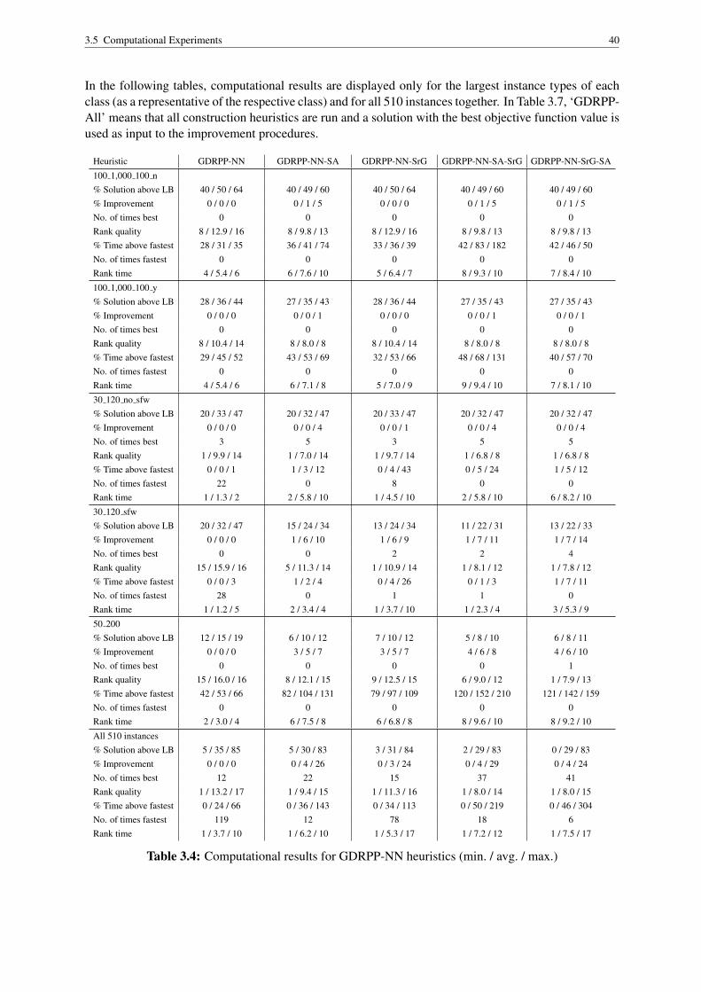
3.5 Computational Experiments 40
In the following tables, computational results are displayed only for the largest instance types of eachclass (as a representative of the respective class) and for all 510 instances together. In Table 3.7, ‘GDRPP-All’ means that all construction heuristics are run and a solution with the best objective function value isused as input to the improvement procedures.
Heuristic GDRPP-NN GDRPP-NN-SA GDRPP-NN-SrG GDRPP-NN-SA-SrG GDRPP-NN-SrG-SA
100 1,000 100 n% Solution above LB 40 / 50 / 64 40 / 49 / 60 40 / 50 / 64 40 / 49 / 60 40 / 49 / 60% Improvement 0 / 0 / 0 0 / 1 / 5 0 / 0 / 0 0 / 1 / 5 0 / 1 / 5No. of times best 0 0 0 0 0Rank quality 8 / 12.9 / 16 8 / 9.8 / 13 8 / 12.9 / 16 8 / 9.8 / 13 8 / 9.8 / 13% Time above fastest 28 / 31 / 35 36 / 41 / 74 33 / 36 / 39 42 / 83 / 182 42 / 46 / 50No. of times fastest 0 0 0 0 0Rank time 4 / 5.4 / 6 6 / 7.6 / 10 5 / 6.4 / 7 8 / 9.3 / 10 7 / 8.4 / 10
100 1,000 100 y% Solution above LB 28 / 36 / 44 27 / 35 / 43 28 / 36 / 44 27 / 35 / 43 27 / 35 / 43% Improvement 0 / 0 / 0 0 / 0 / 1 0 / 0 / 0 0 / 0 / 1 0 / 0 / 1No. of times best 0 0 0 0 0Rank quality 8 / 10.4 / 14 8 / 8.0 / 8 8 / 10.4 / 14 8 / 8.0 / 8 8 / 8.0 / 8% Time above fastest 29 / 45 / 52 43 / 53 / 69 32 / 53 / 66 48 / 68 / 131 40 / 57 / 70No. of times fastest 0 0 0 0 0Rank time 4 / 5.4 / 6 6 / 7.1 / 8 5 / 7.0 / 9 9 / 9.4 / 10 7 / 8.1 / 10
30 120 no sfw% Solution above LB 20 / 33 / 47 20 / 32 / 47 20 / 33 / 47 20 / 32 / 47 20 / 32 / 47% Improvement 0 / 0 / 0 0 / 0 / 4 0 / 0 / 1 0 / 0 / 4 0 / 0 / 4No. of times best 3 5 3 5 5Rank quality 1 / 9.9 / 14 1 / 7.0 / 14 1 / 9.7 / 14 1 / 6.8 / 8 1 / 6.8 / 8% Time above fastest 0 / 0 / 1 1 / 3 / 12 0 / 4 / 43 0 / 5 / 24 1 / 5 / 12No. of times fastest 22 0 8 0 0Rank time 1 / 1.3 / 2 2 / 5.8 / 10 1 / 4.5 / 10 2 / 5.8 / 10 6 / 8.2 / 10
30 120 sfw% Solution above LB 20 / 32 / 47 15 / 24 / 34 13 / 24 / 34 11 / 22 / 31 13 / 22 / 33% Improvement 0 / 0 / 0 1 / 6 / 10 1 / 6 / 9 1 / 7 / 11 1 / 7 / 14No. of times best 0 0 2 2 4Rank quality 15 / 15.9 / 16 5 / 11.3 / 14 1 / 10.9 / 14 1 / 8.1 / 12 1 / 7.8 / 12% Time above fastest 0 / 0 / 3 1 / 2 / 4 0 / 4 / 26 0 / 1 / 3 1 / 7 / 11No. of times fastest 28 0 1 1 0Rank time 1 / 1.2 / 5 2 / 3.4 / 4 1 / 3.7 / 10 1 / 2.3 / 4 3 / 5.3 / 9
50 200% Solution above LB 12 / 15 / 19 6 / 10 / 12 7 / 10 / 12 5 / 8 / 10 6 / 8 / 11% Improvement 0 / 0 / 0 3 / 5 / 7 3 / 5 / 7 4 / 6 / 8 4 / 6 / 10No. of times best 0 0 0 0 1Rank quality 15 / 16.0 / 16 8 / 12.1 / 15 9 / 12.5 / 15 6 / 9.0 / 12 1 / 7.9 / 13% Time above fastest 42 / 53 / 66 82 / 104 / 131 79 / 97 / 109 120 / 152 / 210 121 / 142 / 159No. of times fastest 0 0 0 0 0Rank time 2 / 3.0 / 4 6 / 7.5 / 8 6 / 6.8 / 8 8 / 9.6 / 10 8 / 9.2 / 10
All 510 instances% Solution above LB 5 / 35 / 85 5 / 30 / 83 3 / 31 / 84 2 / 29 / 83 0 / 29 / 83% Improvement 0 / 0 / 0 0 / 4 / 26 0 / 3 / 24 0 / 4 / 29 0 / 4 / 24No. of times best 12 22 15 37 41Rank quality 1 / 13.2 / 17 1 / 9.4 / 15 1 / 11.3 / 16 1 / 8.0 / 14 1 / 8.0 / 15% Time above fastest 0 / 24 / 66 0 / 36 / 143 0 / 34 / 113 0 / 50 / 219 0 / 46 / 304No. of times fastest 119 12 78 18 6Rank time 1 / 3.7 / 10 1 / 6.2 / 10 1 / 5.3 / 17 1 / 7.2 / 12 1 / 7.5 / 17
Table 3.4: Computational results for GDRPP-NN heuristics (min. / avg. / max.)

3.5 Computational Experiments 41
Heuristic GDRPP-BC GDRPP-BC-SA GDRPP-BC-SrG GDRPP-BC-SA-SrG GDRPP-BC-SrG-SA
100 1,000 100 n% Solution above LB 36 / 52 / 70 34 / 51 / 67 36 / 52 / 70 34 / 51 / 67 34 / 51 / 67% Improvement 0 / 0 / 0 0 / 1 / 3 0 / 0 / 0 0 / 1 / 3 0 / 1 / 3No. of times best 0 0 0 0 0Rank quality 8 / 13.7 / 16 8 / 10.7 / 13 8 / 13.7 / 16 8 / 10.7 / 13 8 / 10.7 / 13% Time above fastest 0 / 0 / 0 4 / 7 / 10 7 / 85 / 180 9 / 16 / 30 12 / 20 / 48No. of times fastest 30 0 0 0 0Rank time 1 / 1.0 / 1 2 / 2.1 / 3 2 / 6.7 / 10 3 / 3.4 / 5 3 / 4.4 / 8
100 1,000 100 y% Solution above LB 28 / 36 / 44 27 / 35 / 43 28 / 36 / 44 27 / 35 / 43 27 / 35 / 43% Improvement 0 / 0 / 0 0 / 0 / 1 0 / 0 / 0 0 / 0 / 1 0 / 0 / 1No. of times best 0 0 0 0 0Rank quality 8 / 10.4 / 14 8 / 8.0 / 8 8 / 10.4 / 14 8 / 8.0 / 8 8 / 8.0 / 8% Time above fastest 0 / 3 / 10 0 / 6 / 28 0 / 89 / 256 0 / 15 / 66 2 / 13 / 37No. of times fastest 16 12 2 2 0Rank time 1 / 1.8 / 4 1 / 1.9 / 5 1 / 7.1 / 10 1 / 3.5 / 8 2 / 3.4 / 5
30 120 no sfw% Solution above LB 20 / 33 / 47 20 / 32 / 47 20 / 33 / 47 20 / 32 / 47 20 / 32 / 47% Improvement 0 / 0 / 0 0 / 0 / 4 0 / 0 / 1 0 / 0 / 4 0 / 0 / 4No. of times best 3 5 3 5 5Rank quality 1 / 9.9 / 14 1 / 7.0 / 14 1 / 9.7 / 14 1 / 6.8 / 8 1 / 6.8 / 8% Time above fastest 1 / 2 / 5 1 / 2 / 5 1 / 2 / 9 1 / 4 / 8 2 / 5 / 18No. of times fastest 0 0 0 0 0Rank time 3 / 5.1 / 9 2 / 4.0 / 10 2 / 4.5 / 9 4 / 7.5 / 10 6 / 7.9 / 10
30 120 sfw% Solution above LB 20 / 32 / 47 15 / 24 / 34 13 / 24 / 34 11 / 22 / 31 13 / 22 / 33% Improvement 0 / 0 / 0 1 / 6 / 10 1 / 6 / 9 1 / 7 / 11 1 / 7 / 14No. of times best 0 0 2 2 4Rank quality 15 / 15.9 / 16 5 / 11.3 / 14 1 / 10.9 / 14 1 / 8.1 / 12 1 / 7.8 / 12% Time above fastest 9 / 11 / 25 9 / 9 / 9 9 / 10 / 17 9 / 11 / 20 10 / 12 / 19No. of times fastest 0 0 0 0 0Rank time 6 / 8.0 / 10 5 / 5.9 / 7 5 / 7.1 / 10 7 / 8.4 / 10 8 / 9.5 / 10
50 200% Solution above LB 25 / 32 / 39 7 / 10 / 14 7 / 11 / 14 6 / 9 / 13 6 / 8 / 11% Improvement 0 / 0 / 0 12 / 17 / 22 11 / 16 / 20 13 / 18 / 23 14 / 18 / 22No. of times best 0 0 0 0 0Rank quality 17 / 17.0 / 17 9 / 13.4 / 15 10 / 14.1 / 15 4 / 9.4 / 14 3 / 8.5 / 13% Time above fastest 0 / 0 / 0 37 / 46 / 70 40 / 104 / 479 79 / 88 / 102 78 / 89 / 99No. of times fastest 30 0 0 0 0Rank time 1 / 1.0 / 1 2 / 2.2 / 4 2 / 5.2 / 10 4 / 4.9 / 6 4 / 5.3 / 6
All 510 instances% Solution above LB 6 / 39 / 109 0 / 30 / 92 4 / 32 / 94 0 / 29 / 92 0 / 30 / 92% Improvement 0 / 0 / 0 0 / 6 / 42 0 / 5 / 44 0 / 7 / 42 0 / 7 / 44No. of times best 12 24 16 45 47Rank quality 1 / 13.7 / 17 1 / 9.8 / 16 1 / 11.8 / 16 1 / 8.2 / 15 1 / 8.2 / 15% Time above fastest 0 / 3 / 94 0 / 13 / 70 0 / 54 / 696 0 / 26 / 215 0 / 25 / 135No. of times fastest 287 26 22 10 3Rank time 1 / 3.2 / 10 1 / 3.8 / 10 1 / 5.4 / 17 1 / 5.4 / 17 1 / 5.8 / 10
Table 3.5: Computational results for GDRPP-BC heuristics (min. / avg. / max.)
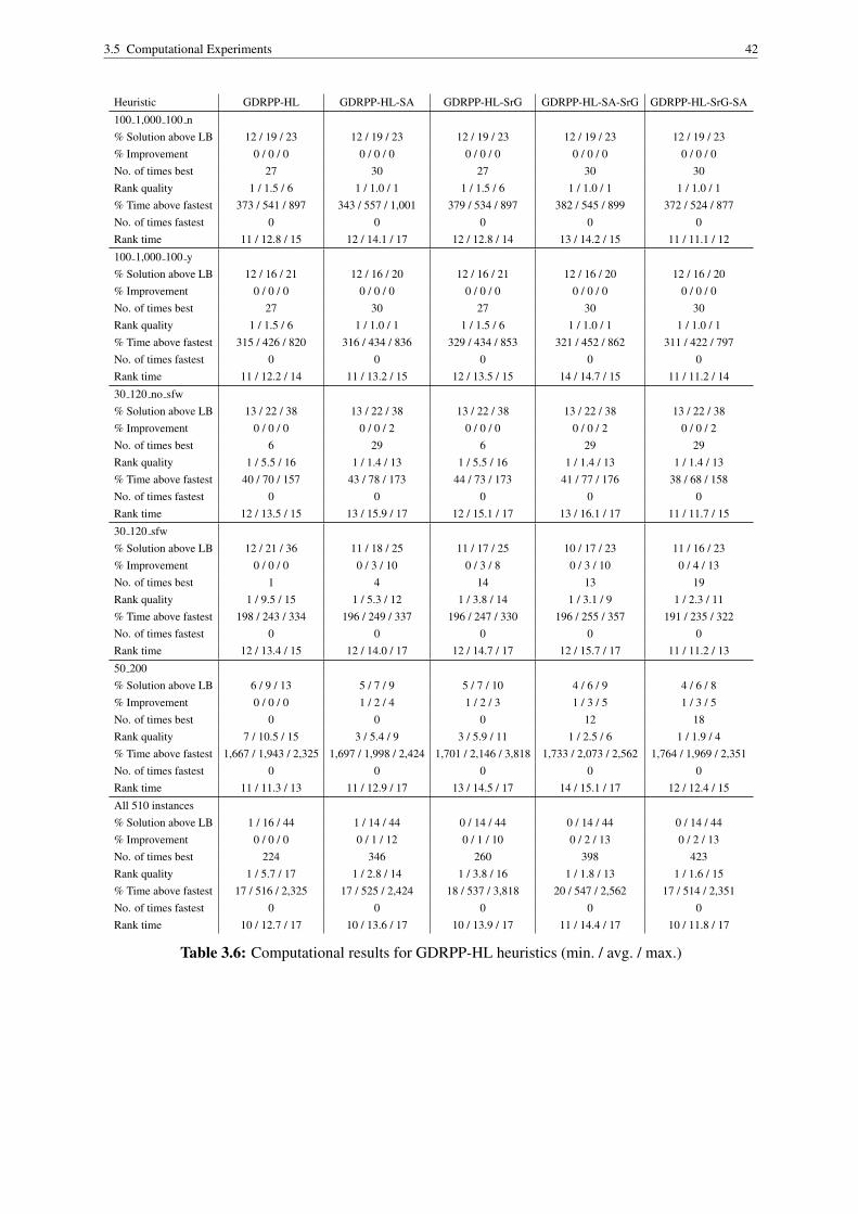
3.5 Computational Experiments 42
Heuristic GDRPP-HL GDRPP-HL-SA GDRPP-HL-SrG GDRPP-HL-SA-SrG GDRPP-HL-SrG-SA
100 1,000 100 n% Solution above LB 12 / 19 / 23 12 / 19 / 23 12 / 19 / 23 12 / 19 / 23 12 / 19 / 23% Improvement 0 / 0 / 0 0 / 0 / 0 0 / 0 / 0 0 / 0 / 0 0 / 0 / 0No. of times best 27 30 27 30 30Rank quality 1 / 1.5 / 6 1 / 1.0 / 1 1 / 1.5 / 6 1 / 1.0 / 1 1 / 1.0 / 1% Time above fastest 373 / 541 / 897 343 / 557 / 1,001 379 / 534 / 897 382 / 545 / 899 372 / 524 / 877No. of times fastest 0 0 0 0 0Rank time 11 / 12.8 / 15 12 / 14.1 / 17 12 / 12.8 / 14 13 / 14.2 / 15 11 / 11.1 / 12
100 1,000 100 y% Solution above LB 12 / 16 / 21 12 / 16 / 20 12 / 16 / 21 12 / 16 / 20 12 / 16 / 20% Improvement 0 / 0 / 0 0 / 0 / 0 0 / 0 / 0 0 / 0 / 0 0 / 0 / 0No. of times best 27 30 27 30 30Rank quality 1 / 1.5 / 6 1 / 1.0 / 1 1 / 1.5 / 6 1 / 1.0 / 1 1 / 1.0 / 1% Time above fastest 315 / 426 / 820 316 / 434 / 836 329 / 434 / 853 321 / 452 / 862 311 / 422 / 797No. of times fastest 0 0 0 0 0Rank time 11 / 12.2 / 14 11 / 13.2 / 15 12 / 13.5 / 15 14 / 14.7 / 15 11 / 11.2 / 14
30 120 no sfw% Solution above LB 13 / 22 / 38 13 / 22 / 38 13 / 22 / 38 13 / 22 / 38 13 / 22 / 38% Improvement 0 / 0 / 0 0 / 0 / 2 0 / 0 / 0 0 / 0 / 2 0 / 0 / 2No. of times best 6 29 6 29 29Rank quality 1 / 5.5 / 16 1 / 1.4 / 13 1 / 5.5 / 16 1 / 1.4 / 13 1 / 1.4 / 13% Time above fastest 40 / 70 / 157 43 / 78 / 173 44 / 73 / 173 41 / 77 / 176 38 / 68 / 158No. of times fastest 0 0 0 0 0Rank time 12 / 13.5 / 15 13 / 15.9 / 17 12 / 15.1 / 17 13 / 16.1 / 17 11 / 11.7 / 15
30 120 sfw% Solution above LB 12 / 21 / 36 11 / 18 / 25 11 / 17 / 25 10 / 17 / 23 11 / 16 / 23% Improvement 0 / 0 / 0 0 / 3 / 10 0 / 3 / 8 0 / 3 / 10 0 / 4 / 13No. of times best 1 4 14 13 19Rank quality 1 / 9.5 / 15 1 / 5.3 / 12 1 / 3.8 / 14 1 / 3.1 / 9 1 / 2.3 / 11% Time above fastest 198 / 243 / 334 196 / 249 / 337 196 / 247 / 330 196 / 255 / 357 191 / 235 / 322No. of times fastest 0 0 0 0 0Rank time 12 / 13.4 / 15 12 / 14.0 / 17 12 / 14.7 / 17 12 / 15.7 / 17 11 / 11.2 / 13
50 200% Solution above LB 6 / 9 / 13 5 / 7 / 9 5 / 7 / 10 4 / 6 / 9 4 / 6 / 8% Improvement 0 / 0 / 0 1 / 2 / 4 1 / 2 / 3 1 / 3 / 5 1 / 3 / 5No. of times best 0 0 0 12 18Rank quality 7 / 10.5 / 15 3 / 5.4 / 9 3 / 5.9 / 11 1 / 2.5 / 6 1 / 1.9 / 4% Time above fastest 1,667 / 1,943 / 2,325 1,697 / 1,998 / 2,424 1,701 / 2,146 / 3,818 1,733 / 2,073 / 2,562 1,764 / 1,969 / 2,351No. of times fastest 0 0 0 0 0Rank time 11 / 11.3 / 13 11 / 12.9 / 17 13 / 14.5 / 17 14 / 15.1 / 17 12 / 12.4 / 15
All 510 instances% Solution above LB 1 / 16 / 44 1 / 14 / 44 0 / 14 / 44 0 / 14 / 44 0 / 14 / 44% Improvement 0 / 0 / 0 0 / 1 / 12 0 / 1 / 10 0 / 2 / 13 0 / 2 / 13No. of times best 224 346 260 398 423Rank quality 1 / 5.7 / 17 1 / 2.8 / 14 1 / 3.8 / 16 1 / 1.8 / 13 1 / 1.6 / 15% Time above fastest 17 / 516 / 2,325 17 / 525 / 2,424 18 / 537 / 3,818 20 / 547 / 2,562 17 / 514 / 2,351No. of times fastest 0 0 0 0 0Rank time 10 / 12.7 / 17 10 / 13.6 / 17 10 / 13.9 / 17 11 / 14.4 / 17 10 / 11.8 / 17
Table 3.6: Computational results for GDRPP-HL heuristics (min. / avg. / max.)

3.5 Computational Experiments 43
Heuristic GDRPP-All-SA-SrG GDRPP-All-SrG-SA
100 1,000 100 n% Solution above LB 12 / 19 / 23 12 / 19 / 23% Improvement 0 / 0 / 0 0 / 0 / 0No. of times best 30 30Rank quality 1 / 1.0 / 1 1 / 1.0 / 1% Time above fastest 461 / 615 / 972 459 / 613 / 968No. of times fastest 0 0Rank time 16 / 16.7 / 17 15 / 16.1 / 17
100 1,000 100 y% Solution above LB 12 / 16 / 20 12 / 16 / 20% Improvement 0 / 0 / 0 0 / 0 / 0No. of times best 30 30Rank quality 1 / 1.0 / 1 1 / 1.0 / 1% Time above fastest 418 / 541 / 920 417 / 541 / 916No. of times fastest 0 0Rank time 16 / 16.7 / 17 16 / 16.2 / 17
30 120 no sfw% Solution above LB 13 / 22 / 38 13 / 22 / 38% Improvement 0 / 0 / 2 0 / 0 / 2No. of times best 30 30Rank quality 1 / 1.0 / 1 1 / 1.0 / 1% Time above fastest 40 / 56 / 81 40 / 56 / 80No. of times fastest 0 0Rank time 11 / 12.9 / 15 11 / 12.5 / 16
30 120 sfw% Solution above LB 10 / 17 / 23 11 / 16 / 23% Improvement 0 / 3 / 10 0 / 4 / 13No. of times best 13 19Rank quality 1 / 3.1 / 9 1 / 2.3 / 11% Time above fastest 202 / 237 / 282 202 / 237 / 282No. of times fastest 0 0Rank time 12 / 14.6 / 17 11 / 14.3 / 17
50 200% Solution above LB 4 / 6 / 9 4 / 6 / 8% Improvement 1 / 3 / 5 1 / 3 / 5No. of times best 12 18Rank quality 1 / 2.5 / 6 1 / 1.9 / 4% Time above fastest 1,819 / 2,103 / 2,543 1,815 / 2,009 / 2,500No. of times fastest 0 0Rank time 14 / 16.0 / 17 14 / 15.7 / 17
All 510 instances% Solution above LB 0 / 14 / 42 0 / 14 / 42% Improvement 0 / 1 / 13 0 / 2 / 13No. of times best 399 426Rank quality 1 / 1.7 / 12 1 / 1.6 / 11% Time above fastest 18 / 574 / 2,543 18 / 574 / 2,500No. of times fastest 0 0Rank time 10 / 15.5 / 17 10 / 15.3 / 17
Table 3.7: Computational results for GDRPP-All heuristics (min. / avg. / max.)
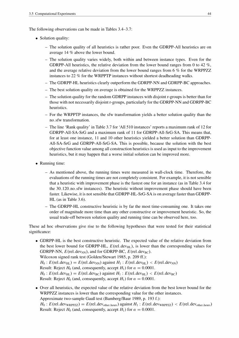
3.5 Computational Experiments 44
The following observations can be made in Tables 3.4–3.7:
• Solution quality:
– The solution quality of all heuristics is rather poor. Even the GDRPP-All heuristics are onaverage 14 % above the lower bound.
– The solution quality varies widely, both within and between instance types. Even for theGDRPP-All heuristics, the relative deviation from the lower bound ranges from 0 to 42 %,and the average relative deviation from the lower bound ranges from 6 % for the WRPPZZinstances to 22 % for the WRPPTP instances without shortest deadheading walks.
– The GDRPP-HL heuristics clearly outperform the GDRPP-NN and GDRPP-BC approaches.
– The best solution quality on average is obtained for the WRPPZZ instances.
– The solution quality for the random GDRPP instances with disjoint r-groups is better than forthose with not necessarily disjoint r-groups, particularly for the GDRPP-NN and GDRPP-BCheuristics.
– For the WRPPTP instances, the sfw transformation yields a better solution quality than theno sfw transformation.
– The line ‘Rank quality’ in Table 3.7 for ‘All 510 instances’ reports a maximum rank of 12 forGDRPP-All-SA-SrG and a maximum rank of 11 for GDRPP-All-SrG-SA. This means that,for at least one instance, 11 and 10 other heuristics yielded a better solution than GDRPP-All-SA-SrG and GDRPP-All-SrG-SA. This is possible, because the solution with the bestobjective function value among all construction heuristics is used as input to the improvementheuristics, but it may happen that a worse initial solution can be improved more.
• Running time:
– As mentioned above, the running times were measured in wall-clock time. Therefore, theevaluations of the running times are not completely consistent. For example, it is not sensiblethat a heuristic with improvement phase is the fastest one for an instance (as in Table 3.4 forthe 30 120 no sfw instances). The heuristic without improvement phase should have beenfaster. Likewise, it is not sensible that GDRPP-HL-SrG-SA is on average faster than GDRPP-HL (as in Table 3.6).
– The GDRPP-HL constructive heuristic is by far the most time-consuming one. It takes oneorder of magnitude more time than any other constructive or improvement heuristic. So, theusual trade-off between solution quality and running time can be observed here, too.
These ad hoc observations give rise to the following hypotheses that were tested for their statisticalsignificance:
• GDRPP-HL is the best constructive heuristic. The expected value of the relative deviation fromthe best lower bound for GDRPP-HL, E(rel devHL), is lower than the corresponding values forGDRPP-NN, E(rel devNN), and for GDRPP-BC, E(rel devBC).Wilcoxon signed rank test (Golden/Stewart 1985, p. 209 ff.):H0 : E(rel devHL) = E(rel devNN) against H1 : E(rel devHL) < E(rel devNN)
Result: Reject H0 (and, consequently, accept H1) for α = 0.0001.H0 : E(rel devHL) = E(rel devBC) against H1 : E(rel devHL) < E(rel devBC)
Result: Reject H0 (and, consequently, accept H1) for α = 0.0001.
• Over all heuristics, the expected value of the relative deviation from the best lower bound for theWRPPZZ instances is lower than the corresponding value for the other instances.Approximate two-sample Gauß test (Bamberg/Baur 1989, p. 193 f.):H0 : E(rel devWRPPZZ) = E(rel devother heurs) against H1 : E(rel devWRPPZZ) < E(rel devother heurs)
Result: Reject H0 (and, consequently, accept H1) for α = 0.0001.

3.5 Computational Experiments 45
• Over all heuristics, the expected value of the relative deviation from the best lower bound for thesfw transformation of the WRPPTP instances into GDRPP instances, E(WRPPTP-SFW), is lowerthan the corresponding expected value for the no sfw transformation, E(WRPPTP-No-SFW).Wilcoxon signed rank test:H0 : E(WRPPTP-SFW) = E(WRPPTP-No-SFW) againstH1 : E(WRPPTP-SFW) < E(WRPPTP-No-SFW)
Reject H0 (and, consequently, accept H1) for α = 0.0001.
Hence, all three hypotheses could be verified at a very high level of significance.
All transformed WRPPTP instances have disjoint r-groups, so for these instances as well as for the ran-dom GDRPP instances with disjoint r-groups, the results with respect to solution quality are identical forthe GDRPP-NN and the GDRPP-BC heuristics.
Why are the results obtained with the sfw transformation better than those obtained with the no sfwtransformation? It follows from the construction of the GDRPP-NN heuristic that the solutions for trans-formed WRPPTP instances will be the same for the sfw and the no sfw transformation. Also, the resultswith the GDRPP-HL heuristic were very similar for the sfw and the no sfw instances. This means thatthe sfw transformation leaves more opportunities for the improvement heuristics. This is probably dueto the following fact: When an arc is removed in the no sfw transformation, the solution cycle is closedagain by the arcs on the shortest path from the head of the preceding r-group arc to the tail of the suc-ceeding r-group arc. If this path contains the removed arc, the latter will immediately be inserted againand the solution will remain unchanged. However, when an arc is removed in the sfw transformation, thecycle is closed by the non-r-group deadheading arc representing the shortest path from the head of thepreceding r-group arc to the tail of the succeeding r-group arc. If the removed arc at its former positionin the cycle was the best way to cover its r-group, it will be inserted again at this position. If it was not,a better arc will be inserted at a better position.
The running times of the heuristics ranged from 200 milliseconds to slightly less than one minute. Theaverage over all 510 instances was 2.46 seconds for the ten combinations of GDRPP-NN and GDRPP-BC with improvement heuristics (Tables 3.4 and 3.5), and 7.82 seconds for the seven combinations ofGDRPP-HL and GDRPP-All with improvement heuristics (Tables 3.6 and 3.7). However, the implemen-tation of the heuristics was not optimized for speed, so it should be possible to reduce the running timesby one order of magnitude.
Figure 3.16 depicts a Pareto diagram of the 17 considered combinations of constructive and improvementheuristics. There are six Pareto-optimal combinations. GDRPP-HL-SrG-SA is best with respect tosolution quality, GDRPP-BC is best with respect to running time. No combination comes close to the‘perfect’ heuristic, whose position is marked with an asterisk, and the relatively sharp trade-off betweensolution quality and running time becomes visible: Most combinations are quite close to the line from(1; 17) (best rank with respect to time, last rank with respect to quality) to (17; 1) (vice versa). Alongthis line, any increase in solution quality leads to an equivalent increase in running time. On the otherhand, almost all combinations are below this line, which means that the trade-off is less than 1-to-1.
3.5.3.3 Results for the Branch-and-Cut Algorithm
To test the usefulness of the δi cuts and the upper bounding by the heuristic solution, all test instanceswere tackled with the following four set-ups:
(i) no cuts, no upper bounding
(ii) with δi cuts, no upper bounding
(iii) no δi cuts, with upper bounding
(iv) with δi cuts, with upper bounding

3.5 Computational Experiments 46
................ ............
Rank time
................
............Rank quality
×...................
NN
×
×
×
........
........
.
NN-SA-SrG
×
×...............BC
×...................
BC-SA
×
×...................
BC-SA-SrG×
×
××
××...................
HL-SrG-SA××
∗
...................................................................................................................................................................................................................................................................................................................................................................................................................
Figure 3.16: Pareto diagram GDRPP heuristics
The following table presents the computational results obtained with the branch-and-cut algorithm. Theline headings in the table have the following meanings:
• No. of tried / feasible / optimal: number of instances that were tackled with the respective branch-and-cut set-up, number of instances for which a feasible solution was found (before reaching thetime limit or running out of memory), and number of instances that were solved to optimality
• % Gap at root: percentage by which heuristic upper bound (HU B) exceeds lower bound at theroot vertex of the branch-and-bound tree (RL B): (HU B − RL B)/ RL B · 100
• % Gap at end: percentage by which best feasible solution (B F S) exceeds best lower bound atthe end of the optimization (BL B) (zero if optimal solution is found, not counted if no feasiblesolution is found): (B F S − BL B)/ BL B · 100
• No. of times UB pruned: number of times a vertex of the branch-and-bound tree could be prunedbecause of the heuristic upper bound
In all columns, only the running times for the branch-and-cut algorithm itself are indicated; the timeneeded to compute the upper bounds is not included in the running times given in the pertinent columns.As before, the running times were measured in wall-clock time, and hence, there are again some smallinconsistencies.
No cuts, no UB Cuts, no UB No cuts, UB Cuts, UB
50 500 10 nNo. of vertices / arcs / r-groups 58 / 516 / 10No. of flow vars. / δi vars. / constraints 516 / 58 / 585No. of tried / feasible / optimal 10 / 10 / 10 10 / 10 / 10 10 / 10 / 10 10 / 10 / 10Running time [s] 0 / 53 / 257 0 / 40 / 261 0 / 44 / 146 0 / 26 / 125% Gap at root – – 3 / 15 / 25 7 / 15 / 25% Gap at end 0 / 0 / 0 0 / 0 / 0 0 / 0 / 0 0 / 0 / 0No. of times UB pruned – – 0 / 45 / 231 0 / 8 / 62No. of B&B vertices 1 / 595 / 1,884 1 / 212 / 1,168 1 / 569 / 1,980 1 / 154 / 473No. of separated SECs 4 / 994 / 3,579 2 / 989 / 3,921 4 / 701 / 2,126 2 / 775 / 2,833
50 500 10 yNo. of vertices / arcs / r-groups 55 / 510 / 10No. of flow vars. / δi vars. / constraints 510 / 55 / 576No. of tried / feasible / optimal 10 / 10 / 10 10 / 10 / 10 10 / 10 / 10 10 / 10 / 10Running time [s] 0 / 32 / 260 0 / 19 / 130 0 / 38 / 263 0 / 23 / 188% Gap at root – – 6 / 14 / 27 5 / 14 / 25% Gap at end 0 / 0 / 0 0 / 0 / 0 0 / 0 / 0 0 / 0 / 0No. of times UB pruned – – 0 / 15 / 115 0 / 7 / 40No. of B&B vertices 1 / 375 / 2,180 1 / 122 / 699 1 / 428 / 2,180 1 / 130 / 839No. of separated SECs 0 / 480 / 3,097 1 / 549 / 2,778 0 / 540 / 3,097 1 / 543 / 3,550
(continued on next page)

3.5 Computational Experiments 47
(continued from previous page)No cuts, no UB Cuts, no UB No cuts, UB Cuts, UB
50 500 15 nNo. of vertices / arcs / r-groups 58 / 516 / 15No. of flow vars. / δi vars. / constraints 516 / 58 / 589No. of tried / feasible / optimal 10 / 10 / 10 10 / 10 / 10 10 / 10 / 10 10 / 10 / 10Running time [s] 0 / 22 / 125 0 / 192 / 753 0 / 61 / 319 0 / 99 / 601% Gap at root – – 11 / 18 / 36 11 / 18 / 34% Gap at end 0 / 0 / 0 0 / 0 / 0 0 / 0 / 0 0 / 0 / 0No. of times UB pruned – – 0 / 36 / 295 0 / 2 / 15No. of B&B vertices 1 / 255 / 1,124 1 / 268 / 824 1 / 337 / 1,552 1 / 204 / 630No. of separated SECs 27 / 518 / 2,610 17 / 2,582 / 7,819 27 / 698 / 2,881 17 / 1,739 / 7,819
50 500 15 yNo. of vertices / arcs / r-groups 55 / 510 / 15No. of flow vars. / δi vars. / constraints 510 / 55 / 580No. of tried / feasible / optimal 10 / 10 / 10 10 / 10 / 10 10 / 10 / 10 10 / 10 / 10Running time [s] 0 / 6 / 22 0 / 10 / 29 0 / 6 / 15 0 / 10 / 29% Gap at root – – 5 / 14 / 29 5 / 14 / 28% Gap at end 0 / 0 / 0 0 / 0 / 0 0 / 0 / 0 0 / 0 / 0No. of times UB pruned – – 0 / 2 / 24 0 / 3 / 33No. of B&B vertices 1 / 114 / 461 1 / 81 / 327 1 / 108 / 461 1 / 80 / 327No. of separated SECs 9 / 247 / 837 16 / 484 / 1,199 9 / 231 / 837 16 / 474 / 1,199
50 500 20 nNo. of vertices / arcs / r-groups 58 / 515 / 20No. of flow vars. / δi vars. / constraints 515 / 58 / 594No. of tried / feasible / optimal 10 / 10 / 10 10 / 10 / 10 10 / 10 / 10 10 / 10 / 10Running time [s] 0 / 11 / 44 1 / 108 / 705 0 / 10 / 44 1 / 68 / 350% Gap at root – – 5 / 16 / 31 5 / 16 / 31% Gap at end 0 / 0 / 0 0 / 0 / 0 0 / 0 / 0 0 / 0 / 0No. of times UB pruned – – 0 / 0 / 4 0 / 6 / 49No. of B&B vertices 1 / 247 / 1,076 1 / 302 / 1,060 1 / 226 / 1,076 1 / 259 / 751No. of separated SECs 11 / 284 / 1,051 44 / 2,017 / 9,013 11 / 276 / 1,051 44 / 1,472 / 4,600
50 500 20 yNo. of vertices / arcs / r-groups 54 / 508 / 20No. of flow vars. / δi vars. / constraints 508 / 54 / 584No. of tried / feasible / optimal 10 / 10 / 10 10 / 10 / 10 10 / 10 / 10 10 / 10 / 10Running time [s] 1 / 46 / 388 1 / 9 / 33 1 / 35 / 258 1 / 11 / 42% Gap at root – – 5 / 16 / 29 5 / 16 / 29% Gap at end 0 / 0 / 0 0 / 0 / 0 0 / 0 / 0 0 / 0 / 0No. of times UB pruned – – 0 / 3 / 15 0 / 0 / 3No. of B&B vertices 7 / 999 / 8,662 1 / 48 / 158 7 / 878 / 7,142 1 / 51 / 188No. of separated SECs 0 / 265 / 1,380 1 / 337 / 1,331 0 / 302 / 1,663 1 / 355 / 1,331
50 500 25 nNo. of vertices / arcs / r-groups 58 / 515 / 25No. of flow vars. / δi vars. / constraints 515 / 58 / 599No. of tried / feasible / optimal 30 / 30 / 30 30 / 30 / 28 30 / 30 / 29 30 / 30 / 29Running time [s] 0 / 85 / 1,892 0 / 458 / 3,931 0 / 151 / 3,900 0 / 418 / 3,900% Gap at root – – 1 / 16 / 24 1 / 16 / 24% Gap at end 0 / 0 / 0 0 / 1 / 16 0 / 1 / 30 0 / 0 / 8No. of times UB pruned – – 0 / 20 / 556 0 / 7 / 160No. of B&B vertices 1 / 482 / 7,078 1 / 639 / 3,173 1 / 454 / 6,255 1 / 697 / 3,173No. of separated SECs 0 / 771 / 7,266 1 / 3,354 / 22,415 0 / 807 / 8,467 1 / 3,064 / 15,013
(continued on next page)
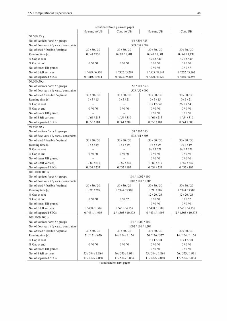
3.5 Computational Experiments 48
(continued from previous page)No cuts, no UB Cuts, no UB No cuts, UB Cuts, UB
50 500 25 yNo. of vertices / arcs / r-groups 54 / 509 / 25No. of flow vars. / δi vars. / constraints 509 / 54 / 589No. of tried / feasible / optimal 30 / 30 / 30 30 / 30 / 30 30 / 30 / 30 30 / 30 / 30Running time [s] 0 / 41 / 755 0 / 93 / 1,901 0 / 47 / 1,001 0 / 67 / 1,132% Gap at root – – 4 / 15 / 29 4 / 15 / 29% Gap at end 0 / 0 / 0 0 / 0 / 0 0 / 0 / 0 0 / 0 / 0No. of times UB pruned – – 0 / 0 / 6 0 / 0 / 7No. of B&B vertices 1 / 489 / 6,501 1 / 332 / 5,267 1 / 535 / 8,144 1 / 262 / 3,162No. of separated SECs 0 / 410 / 4,914 0 / 893 / 9,203 0 / 390 / 5,120 0 / 866 / 8,393
50 500 50 nNo. of vertices / arcs / r-groups 52 / 503 / 50No. of flow vars. / δi vars. / constraints 503 / 52 / 606No. of tried / feasible / optimal 30 / 30 / 30 30 / 30 / 30 30 / 30 / 30 30 / 30 / 30Running time [s] 0 / 5 / 15 0 / 5 / 21 0 / 5 / 15 0 / 5 / 21% Gap at root – – 10 / 17 / 43 9 / 17 / 43% Gap at end 0 / 0 / 0 0 / 0 / 0 0 / 0 / 0 0 / 0 / 0No. of times UB pruned – – 0 / 0 / 0 0 / 0 / 0No. of B&B vertices 1 / 66 / 215 1 / 54 / 319 1 / 66 / 215 1 / 54 / 319No. of separated SECs 0 / 56 / 184 0 / 61 / 305 0 / 56 / 184 0 / 61 / 305
50 500 50 yNo. of vertices / arcs / r-groups 51 / 502 / 50No. of flow vars. / δi vars. / constraints 502 / 51 / 605No. of tried / feasible / optimal 30 / 30 / 30 30 / 30 / 30 30 / 30 / 30 30 / 30 / 30Running time [s] 0 / 5 / 29 0 / 4 / 19 0 / 5 / 29 0 / 4 / 19% Gap at root – – 9 / 15 / 21 9 / 15 / 21% Gap at end 0 / 0 / 0 0 / 0 / 0 0 / 0 / 0 0 / 0 / 0No. of times UB pruned – – 0 / 0 / 0 0 / 0 / 0No. of B&B vertices 1 / 80 / 612 1 / 59 / 342 1 / 80 / 612 1 / 59 / 342No. of separated SECs 0 / 34 / 253 0 / 32 / 197 0 / 34 / 253 0 / 32 / 197
100 1000 100 nNo. of vertices / arcs / r-groups 101 / 1,002 / 100No. of flow vars. / δi vars. / constraints 1,002 / 101 / 1,205No. of tried / feasible / optimal 30 / 30 / 30 30 / 30 / 29 30 / 30 / 30 30 / 30 / 29Running time [s] 1 / 96 / 299 1 / 394 / 3,900 1 / 93 / 287 1 / 394 / 3,900% Gap at root – – 12 / 20 / 25 12 / 20 / 25% Gap at end 0 / 0 / 0 0 / 0 / 2 0 / 0 / 0 0 / 0 / 2No. of times UB pruned – – 0 / 0 / 0 0 / 0 / 0No. of B&B vertices 1 / 408 / 1,586 1 / 651 / 4,158 1 / 408 / 1,586 1 / 651 / 4,158No. of separated SECs 0 / 431 / 1,993 2 / 1,508 / 10,373 0 / 431 / 1,993 2 / 1,508 / 10,373
100 1000 100 yNo. of vertices / arcs / r-groups 101 / 1,002 / 100No. of flow vars. / δi vars. / constraints 1,002 / 101 / 1,204No. of tried / feasible / optimal 30 / 30 / 30 30 / 30 / 30 30 / 30 / 30 30 / 30 / 30Running time [s] 21 / 151 / 650 14 / 164 / 1,154 20 / 136 / 577 14 / 164 / 1,154% Gap at root – – 13 / 17 / 21 13 / 17 / 21% Gap at end 0 / 0 / 0 0 / 0 / 0 0 / 0 / 0 0 / 0 / 0No. of times UB pruned – – 0 / 0 / 0 0 / 0 / 0No. of B&B vertices 55 / 594 / 1,884 56 / 553 / 1,931 55 / 594 / 1,884 56 / 553 / 1,931No. of separated SECs 11 / 452 / 2,068 17 / 584 / 3,834 11 / 452 / 2,068 17 / 584 / 3,834
(continued on next page)

3.5 Computational Experiments 49
(continued from previous page)No cuts, no UB Cuts, no UB No cuts, UB Cuts, UB
10 40 no sfwNo. of vertices / arcs / r-groups 142 / 586 / 19No. of flow vars. / δi vars. / constraints 586 / 142 / 748No. of tried / feasible / optimal 30 / 29 / 29 30 / 30 / 30 30 / 29 / 29 30 / 30 / 30Running time [s] 0 / 53 / 609 0 / 153 / 1,872 0 / 47 / 526 0 / 153 / 1,872% Gap at root – – 6 / 19 / 35 7 / 19 / 35% Gap at end 0 / 0 / 0 0 / 0 / 0 0 / 0 / 0 0 / 0 / 0No. of times UB pruned – – 0 / 0 / 5 0 / 0 / 0No. of B&B vertices 1 / 78 / 603 1 / 128 / 795 1 / 78 / 610 1 / 128 / 795No. of separated SECs 20 / 905 / 5,959 21 / 1,499 / 9,940 20 / 884 / 5,351 21 / 1,499 / 9,940
10 40 sfwNo. of vertices / arcs / r-groups 69 / 1,203 / 19No. of flow vars. / δi vars. / constraints 1,203 / 69 / 1,293No. of tried / feasible / optimal 30 / 30 / 30 30 / 30 / 30 30 / 30 / 30 30 / 30 / 30Running time [s] 0 / 16 / 97 1 / 19 / 234 0 / 13 / 61 1 / 19 / 234% Gap at root – – 3 / 13 / 28 3 / 13 / 28% Gap at end 0 / 0 / 0 0 / 0 / 0 0 / 0 / 0 0 / 0 / 0No. of times UB pruned – – 0 / 0 / 3 0 / 0 / 0No. of B&B vertices 1 / 64 / 767 1 / 57 / 458 1 / 59 / 619 1 / 57 / 458No. of separated SECs 21 / 286 / 1,252 17 / 338 / 2,620 21 / 274 / 890 17 / 338 / 2,620
20 80 no sfwNo. of vertices / arcs / r-groups 282 / 1,197 / 42No. of flow vars. / δi vars. / constraints 1,197 / 282 / 1,522No. of tried / feasible / optimal 30 / 29 / 9 30 / 27 / 10 30 / 29 / 9 30 / 27 / 10Running time [s] 14 / 3,036 / 3,906 7 / 2,934 / 3,906 12 / 3,057 / 3,906 7 / 2,934 / 3,906% Gap at root – – 16 / 24 / 44 16 / 23 / 43% Gap at end 0 / 4 / 13 0 / 4 / 16 0 / 4 / 13 0 / 4 / 16No. of times UB pruned – – 0 / 0 / 0 0 / 0 / 0No. of B&B vertices 34 / 204 / 640 1 / 243 / 753 34 / 213 / 640 1 / 243 / 753No. of separated SECs 65 / 11,336 / 16,808 33 / 10,989 / 18,338 65 / 11,533 / 16,808 33 / 10,989 / 18,338
20 80 sfwNo. of vertices / arcs / r-groups 148 / 5,495 / 42No. of flow vars. / δi vars. / constraints 5,495 / 148 / 5,686No. of tried / feasible / optimal 30 / 30 / 19 30 / 30 / 19 30 / 30 / 19 30 / 30 / 19Running time [s] 9 / 2,101 / 3,917 8 / 1,965 / 3,928 8 / 2,120 / 3,934 8 / 1,965 / 3,928% Gap at root – – 10 / 18 / 29 10 / 18 / 29% Gap at end 0 / 1 / 6 0 / 1 / 8 0 / 1 / 6 0 / 1 / 8No. of times UB pruned – – 0 / 0 / 0 0 / 0 / 0No. of B&B vertices 1 / 354 / 985 1 / 372 / 946 1 / 356 / 985 1 / 372 / 946No. of separated SECs 136 / 5,869 / 10,769 33 / 5,687 / 10,798 136 / 5,912 / 10,617 33 / 5,687 / 10,798
30 120 no sfwNo. of vertices / arcs / r-groups 420 / 1,776 / 59No. of flow vars. / δi vars. / constraints 1,776 / 420 / 2,256No. of tried / feasible / optimal 16 / 10 / 0 30 / 25 / 0 16 / 10 / 0 30 / 25 / 0Running time [s] 3,900 / 3,902 / 3,905 3,900 / 3,905 / 3,933 3,900 / 3,902 / 3,905 3,900 / 3,905 / 3,933% Gap at root – – 16 / 24 / 38 14 / 23 / 38% Gap at end 3 / 8 / 11 0 / 10 / 25 3 / 8 / 11 0 / 10 / 25No. of times UB pruned – – 0 / 0 / 0 0 / 0 / 0No. of B&B vertices 41 / 97 / 289 35 / 106 / 238 41 / 97 / 289 35 / 106 / 238No. of separated SECs 7,633 / 10,815 / 12,753 7,548 / 11,311 / 14,777 7,633 / 10,815 / 12,753 7,548 / 11,311 / 14,777
(continued on next page)

3.5 Computational Experiments 50
(continued from previous page)No cuts, no UB Cuts, no UB No cuts, UB Cuts, UB
30 120 sfwNo. of vertices / arcs / r-groups 207 / 10,696 / 59No. of flow vars. / δi vars. / constraints 10,696 / 207 / 10,963No. of tried / feasible / optimal 30 / 24 / 5 30 / 19 / 5 30 / 24 / 5 30 / 19 / 5Running time [s] 736 / 3,434 / 3,975 742 / 3,373 / 3,985 736 / 3,434 / 3,975 742 / 3,373 / 3,985% Gap at root – – 11 / 18 / 25 12 / 19 / 25% Gap at end 0 / 3 / 10 0 / 4 / 12 0 / 3 / 10 0 / 4 / 12No. of times UB pruned – – 0 / 0 / 0 0 / 0 / 0No. of B&B vertices 41 / 239 / 640 33 / 191 / 459 41 / 239 / 640 33 / 191 / 459No. of separated SECs 1,593 / 6,965 / 10,136 2,016 / 6,621 / 10,061 1,593 / 6,965 / 10,136 2,016 / 6,621 / 10,061
30 100No. of vertices / arcs / r-groups 31 / 371 / 97No. of flow vars. / δi vars. / constraints 371 / 31 / 500No. of tried / feasible / optimal 30 / 30 / 30 30 / 30 / 30 30 / 30 / 30 30 / 30 / 30Running time [s] 0 / 7 / 48 0 / 4 / 26 0 / 6 / 41 0 / 4 / 26% Gap at root – – 2 / 6 / 9 2 / 6 / 9% Gap at end 0 / 0 / 0 0 / 0 / 0 0 / 0 / 0 0 / 0 / 0No. of times UB pruned – – 0 / 0 / 0 0 / 0 / 0No. of B&B vertices 1 / 487 / 3,834 1 / 314 / 2,351 1 / 487 / 3,834 1 / 314 / 2,351No. of separated SECs 0 / 0 / 3 0 / 0 / 3 0 / 0 / 3 0 / 0 / 3
40 150No. of vertices / arcs / r-groups 41 / 559 / 148No. of flow vars. / δi vars. / constraints 559 / 41 / 749No. of tried / feasible / optimal 30 / 30 / 26 30 / 30 / 26 30 / 30 / 26 30 / 30 / 26Running time [s] 0 / 593 / 3,900 0 / 612 / 3,900 0 / 591 / 3,900 0 / 612 / 3,900% Gap at root – – 4 / 7 / 13 4 / 7 / 12% Gap at end 0 / 0 / 0 0 / 0 / 0 0 / 0 / 0 0 / 0 / 0No. of times UB pruned – – 0 / 0 / 0 0 / 0 / 0No. of B&B vertices 1 / 25,390 / 173,086 1 / 27,081 / 187,357 1 / 26,787 / 196,731 1 / 27,081 / 187,357No. of separated SECs 0 / 0 / 1 0 / 0 / 1 0 / 0 / 1 0 / 0 / 1
50 200No. of vertices / arcs / r-groups 51 / 736 / 195No. of flow vars. / δi vars. / constraints 736 / 51 / 983No. of tried / feasible / optimal 30 / 30 / 21 30 / 30 / 21 30 / 30 / 21 30 / 30 / 21Running time [s] 1 / 1,420 / 3,900 0 / 1,550 / 3,901 1 / 1,419 / 3,901 0 / 1,550 / 3,901% Gap at root – – 4 / 6 / 9 4 / 6 / 9% Gap at end 0 / 0 / 0 0 / 0 / 1 0 / 0 / 0 0 / 0 / 1No. of times UB pruned – – 0 / 0 / 0 0 / 0 / 0No. of B&B vertices 10 / 39,842 / 119,503 1 / 43,410 / 111,369 10 / 40,079 / 123,005 1 / 43,410 / 111,369No. of separated SECs 0 / 0 / 1 0 / 0 / 1 0 / 0 / 1 0 / 0 / 1
All 510 instancesNo. of vertices / arcs / r-groups 113 / 1,628 / 62No. of flow vars. / δi vars. / constraints 1,628 / 113 / 1,805No. of tried / feasible / optimal 496 / 482 / 409 510 / 491 / 408 496 / 482 / 408 510 / 491 / 409Running time [s] 0 / 723 / 3,975 0 / 829 / 3,985 0 / 728 / 3,975 0 / 823 / 3,985% Gap at root – – 1 / 15 / 44 1 / 15 / 43% Gap at end 0 / 1 / 13 0 / 1 / 25 0 / 1 / 30 0 / 1 / 25No. of times UB pruned – – 0 / 3 / 556 0 / 1 / 160No. of B&B vertices 1 / 4,333 / 173,086 1 / 4,547 / 187,357 1 / 4,435 / 196,731 1 / 4,543 / 187,357No. of separated SECs 0 / 1,883 / 16,808 0 / 2,431 / 22,415 0 / 1,895 / 16,808 0 / 2,379 / 18,338
Table 3.8: Computational results for branch-and-cut algorithm (min. / avg. / max.)

3.5 Computational Experiments 51
The following observations can be made in Table 3.8:
• The difficulty of the instances varies widely. For each instance type (with the exception of the30 120 WRPPTP instances), there are very easy and very hard instances.
• In general, the δi cuts are not useful. Indeed, over all instances, the percentage by which the lowerbound at the root vertex of the branch-and-bound tree when the cuts are used exceeds the lowerbound when they are not used by a negligible 0.02 %. The average running times, number ofvertices in the branch-and-bound trees, and number of separated SECs even increase when thecuts are used, although there are instances types where this is not the case.
• The upper bounding procedure is not helpful for most instances. The quality of the heuristicsolutions is apparently too poor.
• The number of r-groups is not decisive for the difficulty of an instance type. This is in markedcontrast to the results obtained with the exact labelling algorithm and with the results obtained byNoon/Bean 1991 on the GATSP.
• There is no clear evidence that instances with non-disjoint r-groups are more difficult or easierthan instances with disjoint r-groups.
• The computational results by Laporte 1997 and Blais/Laporte 2003 show that instances with manyrequired edges, i.e., instances with a ‘significant generalized component’, are much more difficultto solve with the solution approaches these authors use than instances of ‘purely’ directed problemsare. Although the transformed WRPPZZ instances, which contain a considerable number of r-groups of cardinality greater than one to represent edges and zigzag links, seem to be more difficultthan the random GDRPP instances, this effect is not so evident in the above computational results.
• Similar to the heuristics, also the branch-and-cut algorithm yields much better results for the sfwtransformation of the WRPPTP instances than for the no sfw transformation, even though thenumber of variables and constraints is very much higher with the sfw transformation.
• For the transformed WRPPZZ instances, the number of vertices in the branch-and-bound tree isextremely high and varies enormously. The results for this instance class are already quite good(considering the number of optimally solved instances), but for this class in particular, there seemsto be a great potential for improvement through better lower and upper bounding procedures. Itis also remarkable that there are almost no violated SECs in any of the transformed WRPPZZinstances.
The following table displays the percentage of instances of each type that were solved to optimality bythe branch-and-cut algorithm.
Instance type No cuts, no UB Cuts, no UB No cuts, UB Cuts, UB
50 500 10 n 100 100 100 10050 500 10 y 100 100 100 10050 500 15 n 100 100 100 10050 500 15 y 100 100 100 10050 500 20 n 100 100 100 10050 500 20 y 100 100 100 10050 500 25 n 100 93 97 9750 500 25 y 100 100 100 10050 500 50 n 100 100 100 10050 500 50 y 100 100 100 100100 1000 100 n 100 97 100 97100 1000 100 y 100 100 100 100
(continued on next page)
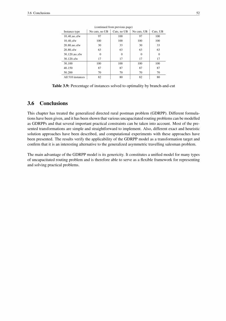
3.6 Conclusions 52
(continued from previous page)Instance type No cuts, no UB Cuts, no UB No cuts, UB Cuts, UB
10 40 no sfw 97 100 97 10010 40 sfw 100 100 100 10020 80 no sfw 30 33 30 3320 80 sfw 63 63 63 6330 120 no sfw 0 0 0 030 120 sfw 17 17 17 17
30 100 100 100 100 10040 150 87 87 87 8750 200 70 70 70 70
All 510 instances 82 80 82 80
Table 3.9: Percentage of instances solved to optimality by branch-and-cut
3.6 Conclusions
This chapter has treated the generalized directed rural postman problem (GDRPP). Different formula-tions have been given, and it has been shown that various uncapacitated routing problems can be modelledas GDRPPs and that several important practical constraints can be taken into account. Most of the pre-sented transformations are simple and straightforward to implement. Also, different exact and heuristicsolution approaches have been described, and computational experiments with these approaches havebeen presented. The results verify the applicability of the GDRPP model as a transformation target andconfirm that it is an interesting alternative to the generalized asymmetric travelling salesman problem.
The main advantage of the GDRPP model is its genericity. It constitutes a unified model for many typesof uncapacitated routing problem and is therefore able to serve as a flexible framework for representingand solving practical problems.

Chapter 4
The Vehicle Routing Problem with Trailersand Transshipments
In this chapter, the vehicle routing problem with trailers and transshipments (VRPTT), a generalizationof the well-known vehicle routing problem (VRP), is introduced. This problem possesses some inter-esting characteristics which have not yet been treated in the literature. In the VRPTT, the vehicle fleetconsists of autonomous vehicles able to move on their own, and of non-autonomous vehicles which mustbe accompanied by an autonomous vehicle to be able to move. Moreover, both autonomous and non-autonomous vehicles are either collection or support vehicles. Collection vehicles are used to collect thesupplies of the customers. Support vehicles are used as mobile depots by the collection vehicles.
The chapter is structured as follows. In the next section, a detailed description of the VRPTT is given,and, based on this description, the essential new aspects of the VRPTT are identified and discussed.Section 4.2 reviews the relevant literature. In Section 4.3, three formulations for the VRPTT are de-veloped. In Section 4.4, the possibility of solving the VRPTT by branch-and-price and the difficultiesarising in such an approach are evaluated, in Section 4.5, a branch-and-cut algorithm is described, and inSection 4.6, computational experiments with this branch-and-cut algorithm are presented and analyzed.The chapter ends with a conclusion.
4.1 Problem Description
The research on the VRPTT was motivated by the following real-world problem: There is a set ofcustomers with a known, deterministic supply of a single good, a set of service stations necessary forunloading and maintenance, and a set of intermediate locations that may be used for parking and loadtransfer. Service stations may also be used for parking. All customers, service stations and intermediatelocations have an arbitrary number of time windows associated with them. These time windows mayrepresent the same time of day on different days. Some customers may have to be visited more thanonce. The supply of a customer is the same on each visit. There may be restrictions on the minimaltime between two consecutive visits at a customer, as well as restrictions specifying the number of visitsthat must occur in a subset of a customer’s time windows. To do the collecting of the good, a fleet ofheterogeneous, limited-capacity vehicles stationed at vehicle depots is available.
There are six main criteria in which the vehicles differ:
(i) First of all, the fleet is comprised of lorries and trailers. On a more abstract level, one can say thatthe fleet consists of two types of vehicle: Autonomous ones, able to move in time and space ontheir own (the lorries), and non-autonomous ones, able to move in time on their own, but requiringan autonomous object to move in space (the trailers).
53

4.1 Problem Description 54
(ii) Second, the lorries may be technically equipped to service customers (collection lorries) or not(support lorries).
(iii) Third, each vehicle may have a different capacity. There may be support lorries with a capacity ofzero. All trailers and all collection lorries have positive capacity.
(iv) Fourth, each vehicle may have different fixed and variable costs. If a vehicle is not used, its fixedcosts are not incurred.
(v) Fifth, the collection lorries may have different load transfer times. This is the time necessary tocollect a given amount of load at a customer or to transfer load to another vehicle.
(vi) Sixth, the collection lorries may be subject to accessibility constraints, i.e., they may not be al-lowed to visit some customers. The driving speeds are assumed to be identical for all lorries,whether or not they pull a trailer, and whether or not they carry load.
Figure 4.1 depicts the four relevant types of vehicle as they are encountered on European streets andmotorways. A lorry with an attached trailer is referred to as a lorry-trailer combination (LTC). Typically,lorries able to form jointed lorry-trailer combinations are used as collection lorries, and saddle lorries(which have a capacity of zero) are used as support lorries.
Jointed lorry-trailer combination
Lorry
.......................................................................................................................................................................... .....................................................................................................................................................................................
........
........
........
........
........
........
........
....................................................................................................................................................................................................................................................................................................... ......................................
.......
Drawbar trailer
............................................................................................................................................................................................................................................................................................................................................................................................................................................................................................................................................................................................. ......................................
....... ...................................................................................
.......
Saddle lorry-trailer combination
Saddle lorry
............................................................................................................................................................................ ............................................................................................................................
....... .............................................
Saddle trailer
.................................................................................................................................................................................................................................................................................................................................................................................................................................................................................................................................................................................................................................................................................................................................................................. ... ......................................
..........................................................................................
.......
Figure 4.1: VRPTT fleet
Essentially, the trailers and the support vehicles are used to extend the capacity of the collection lorries,so that the latter need not go to an unloading station so often. Obviously, for a trailer to be useful, itmust be pulled by a lorry. However, not every combination of lorry and trailer is allowed. Trailers whichcan be pulled only by support lorries are called support trailers, the others are called collection trail-ers. Support vehicles are simply subject to special accessibility constraints at customers. In principle,a collection vehicle can also work as a pure support vehicle, but not the other way round. However, acollection lorry would never be used as a pure support lorry, because a pure support lorry is considerablycheaper. Moreover, the distinction between collection and support vehicles is really not a gradual one,because load transfer locations may be visited by both types of vehicle, but to perform a load transfer,(the technical equipment of) a collection lorry is needed.
Intermediate locations can be used either for parking (parking locations) or for load transfer (load trans-fer locations or transshipment locations).
There is no fixed depot for a vehicle. A vehicle may start its itinerary at any depot. At the end of theplanning horizon, it always returns to the depot it started from. As with intermediate locations, there aretwo types of depot. Parking depots can be used only for parking a vehicle. Transshipment depots offerthe additional possibility of transferring load to a vehicle which is still in the depot.
Using a parking or transshipment location or depot may incur fixed setup costs per vehicle. Typically,these costs are zero for using parking locations or depots. Service stations do not incur setup costs.
Transshipment locations, transshipment depots and service stations have two types of time window: Thevisiting time windows determine the times when these locations may be used for parking, the service time

4.1 Problem Description 55
windows determine the times when load transfers, respectively, unloading or maintenance, are allowed.The visiting time windows contain the service time windows at the respective locations, i.e., load trans-fers, unloading and maintenance are allowed only at times when parking is allowed also.
Coupling and decoupling a trailer incurs certain costs; fleet owners, dispatchers and drivers consider itundesirable to separate a lorry and a trailer ‘too often’. The coupling and decoupling process takes time,but this time is negligible compared to the total driving and loading time.
Customers that can only be visited by a lorry without a trailer (a single lorry) are called lorry cus-tomers. The other customers, which can be visited by a lorry with or without a trailer, are called trailercustomers. As mentioned above, there may be additional vehicle-specific accessibility constraints atcustomers. Split collection is not allowed; hence, there are no customers with a supply exceeding thecapacity of the largest lorry (or lorry-trailer combination, in the case of trailer customers). The statementthat split collection is not allowed holds for individual customers. However, it is sometimes useful toperform a customer aggregation when modelling a real-world problem, in particular when the number ofindividual customers is too large from a computational point of view, and when the customer locationsform clearly separable clusters. In practice, split collection of these aggregated customers is allowed, butthis is not considered here.
The vehicles are used as follows. The standard case is a collection lorry with a trailer. Most customersare lorry customers, so normally the trailer is parked at an intermediate location and the lorry does somecollecting. Then, it either transfers its load to the trailer and continues collecting, or re-couples the trailer,parks it elsewhere, decouples, and does some more collecting before transferring load. When a trailercustomer is visited by a lorry with a trailer, the supply of the customer can directly be loaded completelyor partly into the trailer, and at most customers, any additional load the lorry has already collected can betransferred from lorry to trailer at such a location, too. (Some customers, though, may not want any kindof unnecessary operation performed on their premises.) After collecting at least one customer’s supply,both the lorry and the trailer go to an unloading station for unloading. They may then start another tour.In addition, a collection lorry may also operate singly.
There is no fixed assignment of a trailer to a lorry. Any lorry may pull any compatible trailer for sometime. What is more, any vehicle may transfer load to any other vehicle. In order to do so, the equipmentof a collection lorry must be used. That is, for a load transfer from a trailer to another trailer or to a sup-port lorry, a collection lorry must be present. For unloading a trailer or a support lorry at an unloadingstation, no collection lorry is necessary. Figure 4.2 depicts a possible route plan with three collectionlorries and one trailer. In the plan, lorry 1, together with the trailer, starts at the depot, goes to a trans-shipment location, decouples the trailer there, visits two lorry customers, returns to the trailer, transferssome load, leaves the trailer there and returns to the depot via some lorry and some trailer customers.Lorry 2 starts at the depot, visits some lorry customers, couples the trailer (after lorry 1 has performed itsload transfer), visits a trailer customer, decouples the trailer at another transshipment location, possiblyperforms a load transfer, visits some lorry customers, returns to the parked trailer, re-couples it and pullsit back to the depot via a trailer customer. Meanwhile, lorry 3 also starts at the depot, visits some lorrycustomers, transfers some load to the trailer while lorry 2 is visiting the three lorry customers bottomright, and returns to the depot via another lorry customer. The two transshipment locations in the centreof the figure are not used.
All vehicles must undergo maintenance a specified number of times. As with consecutive visits to cus-tomers, there are restrictions specifying the minimal and maximal time between two consecutive main-tenance processes. One maintenance process takes an amount of time dependent on the maintenancestation and the vehicle. Some unloading stations, called combi stations, can also be used as mainte-nance stations. At any point in time, only one lorry, trailer, or lorry-trailer combination, can unload atan unloading station or be maintained at a maintenance station. At a combi station, only one type of

4.1 Problem Description 56
ppppppppppppppppppppppppppppppppppppppppppppppppp
pppppppppppppppppppppppppppppppppppppppppppppppppppppppppppppppppppppppppppppppppppppppppppppppppppppppppppp
pppppppppppppppppppppppppppppppppppppppppppppppppppppppppppppppppppppppppppppppppppppppppppppppppppppppppppp
pppppppppppppppppppppppppppppppppppppppppppppppppppppppppppppppppppppppppppppppppppppppp ppppppppppppppppppppppppppppppppppppppppppppppppppppppppppppppppppppppppppppppppppppppppppppppppppppppppppppppppppppppppppppppppppppppppppppppppppppppppppppppppppppppppppppppppppppppppppppppppppppp pppppppppppp pppppppppppppppppppppppppppppppppppppppppppppppppppppppppppppppppppppppppppppppppppppppppppppppppppppppppppppppppppppppppppppppppppppppppppppppppppppppppppppp pppppppppppp ppppppppppppppppppppppppppppppppppppppppppppppppppppppppppppppppppppppppppppppppppppppppppppppppppppppppppppppppppppppppppppppppppppppppppppppppppppppppppppppppppppppppppppppppppppppppppppppppppppppppppppppppppppppppppppppppppppppppppppppppppppppppppppppppppppppppppppppppppppppppppppppppppppppppppppppppppppppppppppppppppppppppppppppppppppppppppppppppppppppppppppppppppppppppppppppppppppppppppppppppppppppppppppppppppppppppppppppppppppppppppppppppppppppp
.................................................
.................................................................................................................................................................................................................................................................................................................
......................
......................
.................................................................................................................................................................................................................................................................................................................................................................................. ............ ....................................................................................................
...................................................................................
....
........................................................................
..................................................................
....
.......................................................................................
.....................................
.............
.............
.............
.............
.............
.............
.............
............
.........................
..........................
............
............
.............
.............
.............
.............
.............
........................
............. ............. ............. ............. ............. ............. ............. ....................... ............ ..........................
..........................
.......................... ............ ........
....
............. ............. ............. ............. ............. ............. ............. ............. ............ ............
..............................................
.........................
.............
.....................................
..........................
.......................................
..........................
..........................................................................................................................................................................................................................................
....
. . . . . . . . . . . . . . . . . . . . . . . . . . .. ..
.. .. . . . . ... .
..
..
..
..........................................
N
N
uuuu uu
uuuuu uu u
��
�
� �
�
�
�
��
Depot
Lorry customer
Trailer customer
Transshipment location
Lorry 1
Lorry 2
Lorry 3
Trailer
Figure 4.2: Example of a VRPTT route plan
service (unloading, maintenance) can be performed at a time. To undergo maintenance, a vehicle mustbe empty. A lorry-trailer combination that unloads at an unloading or combi station has a total unloadingtime which is equal to the sum of the unloading times of the lorry and the trailer, but it is technicallypossible to maintain the two vehicles of a lorry-trailer combination at a maintenance or combi station inparallel.
A certain amount of the customers’ supply must be delivered to a certain unloading station. There mayalso be restrictions on the minimum amount of load delivered to an unloading station until a certain pointin time.
Moreover, there may be time intervals where no customer may be visited, i.e., the planning horizon maycontain (at least two) disjoint meta time windows. All customer time windows then lie within one suchmeta time window. There are no intermediate locations or service stations with a time window stretchingover more than two consecutive meta time windows (i.e., stretching over more than one time interval be-tween two meta time windows). Between visits at customers during two consecutive meta time windows,a vehicle must be maintained exactly once and return to the real-world location where its depot is situ-ated. This means that the maintenance frequency of all vehicles equals the number of meta time windows.
The task is to devise routings of minimal total costs for all vehicles (some of which may not be needed),such that the complete supply of all customers is collected and delivered to the unloading stations. Thisincludes the assignment of each vehicle which is used to a depot.
4.1.1 What is New?
Several of the aspects relevant in the problem presented in the previous section are neither novel nor com-plicated. What really is new is the problem as a whole, and, in particular, the simultaneous considerationof the following three points in one problem:
(i) A trailer may be pulled by different lorries on its itinerary.
(ii) Load transfers are possible between arbitrary vehicles.
(iii) There are support vehicles, which cannot visit any customers.
4.1.2 The Central Question
The main difficulty of the problem is the close interdependency between the vehicles: With few excep-tions, the whole road network may be used by all vehicles. The parking and transshipment locations are

4.1 Problem Description 57
there precisely to be visited more than once, and by more than one vehicle. This is not usually the case invehicle routing problems. Moreover, the fact that trailers cannot move on their own and the load transferpossibility give the problem not only a routing, but also a scheduling aspect: The itineraries of trailersand the lorries pulling them and the load transfer processes must be synchronized. All in all, a fourfoldsynchronization of the vehicles is required:
(i) Customer Covering SynchronizationAll customers must be visited exactly the required number of times, and on each visit by exactlyone collection lorry.
(ii) Spacial SynchronizationThe vehicle itineraries must be synchronized, because a trailer must be pulled by a lorry to movein space.
(iii) Temporal Synchronization
• Spacial synchronization evidently implies temporal synchronization for common movementsof a lorry and a trailer.
• In addition, temporal synchronization is necessary at transshipment locations, where vehiclesmay meet that reach these locations from different other locations. A vehicle can perform aload transfer to another vehicle at a transshipment location only if both vehicles are presentat the respective location during the time needed for the load transfer.
(iv) Load SynchronizationFor each transshipment operation, it must be decided how much load is to be transferred. The loadone vehicle unloads is exactly equal to the load the other vehicle receives. No load gets lost.
Temporal and load synchronization are themselves interdependent because of the load-dependent loadtransfer times.
These deliberations are summarized in the central question that must be answered when solving aVRPTT:
Which vehicle transfers how much load when where into which other vehicle?
4.1.3 Potential Savings Through the Use of Trailers
Another question that immediately springs to mind is how much can actually be saved by using trailers.Interestingly, the potential savings are not bounded from above. Consider an instance with one depot, nlorry customers, each with a supply of one, located at a distance of one unit from the depot and arbitrarilyclose to one another, and with one transshipment location arbitrarily close to each of the customers. Ifthere are n identical lorries with fixed costs of zero, distance-dependent costs of one, and a capacity ofone, the optimal solution evidently consists of using one lorry for each customer, and this solution incurscosts of 2n. If there is a trailer with fixed and distance-dependent costs of zero and a capacity of n−1, theoptimal solution consists in using one lorry and the trailer, and this solution incurs costs of 2 (if the loadtransfer speed is assumed to be infinite or if there are no time-dependent costs). As n reaches infinity, sodo the potential absolute savings, and the relative savings reach 100 %.
A less contrived case is given by an instance with one depot, four lorry customers, each with a supplyof six, located at a distance of one unit from the depot and arbitrarily close to one another, and with onetransshipment location arbitrarily close to each of the customers. If the vehicle fleet consists of identicallorries with fixed costs of zero, distance-dependent costs of one and a capacity of ten, the optimal solutionincurs costs of 4 · (1+1) ·1 = 8. If there is a trailer available with fixed costs of zero, distance-dependentcosts of one tenth of the distance-dependent costs of a lorry, and with a capacity of 15, the optimalsolution incurs costs of 2 · 1+ 2 · 0.1 = 2.2, which means a saving of 72.5 %; cf. Figure 4.3. (The case

4.2 Literature Review 58
of a lorry-trailer combination where the lorry has a capacity of about 10 units (tons) and where the trailerhas a capacity of about 15 units (tons) is common in Europe. See also the section on computationalexperiments.)
........
........
........
........
........
........
........
........
........
........
........
........
........
........
........
........
........
........
........
........
........
........
........
........
........
........
........
........
........
........
........
.
............................
................
............
........................................................................... ................ ...........................................................
................
............
............................
N
u uu u�
1
ε
ε
1 Depot
1 Transsh. loc.
4 Lorrycustomers;supply 6
Fleet:4 lorries,capacity 10,fixed costs 0, variable costs 1⇒ minimal cost: 4 · (1+ 1) · 1 = 8One additional trailer,capacity 15,fixed costs 0, variable costs 0.1⇒ minimal cost: 2 · 1+ 2 · 0.1 = 2.2⇒ savings of 72.5 %
Figure 4.3: Potential savings through the use of trailers
4.2 Literature Review
Notwithstanding the considerable potential for cost savings through the use of trailers, the literature onvehicle routing with trailers is scarce. To the best of the author’s knowledge, the subsequent formulationsare the first ones that simultaneously take the above aspects into account. Following is a brief review ofthe few papers there are.
Brunswicker 1986, Vahrenkamp 1989, and Scheuerer 2004 consider the problem of raw milk collectionat farmyards. The milk is collected at storage tanks on the farmyards every or every other day and mustbe transported to dairy plants. Some of the farmyards cannot be visited by a lorry-trailer combinationbecause of space restrictions. The first two authors allow only one transshipment location per trailerand a fixed lorry-trailer assignment. This is not adequate for the VRPTT. Brunswicker 1986 develops aheuristic sequential solution approach for this type of problem (clustering of customers, determinationof one transshipment location per trailer, routing). Vahrenkamp 1989 proceeds similarly.
Semet/Taillard 1993 and Gerdessen 1996 consider the task of food delivery to supermarkets, some ofwhich lie in inner-city areas where there is not enough space for manoeuvring with a lorry-trailer com-bination. Additionally, Gerdessen 1996 considers the distribution of animal food to farmyards, whichessentially is the delivery case corresponding to the raw milk collection case just described.
Gerdessen 1996 also allows only one transshipment location per trailer and a fixed lorry-trailer assign-ment. The paper presents several construction heuristics and intra- and inter-tour exchange improvementprocedures and mentions an unpublished technical report containing an MIP formulation.
Semet/Taillard 1993, Semet 1995, Chao 2002, and Scheuerer 2004 (see also Scheuerer 2006) allow thattrailers be parked several times at different locations, but they identify the potential trailer parking lo-cations with the trailer customers (i.e., any trailer can be parked at any trailer customer location butnowhere else), they assume a fixed lorry-trailer assignment, and they do not allow a load transfer from alorry to a trailer other than its assigned one. Consequently, they do not consider support vehicles. Semet/Taillard 1993 consider time windows and heterogeneous lorries, but identical trailers. Semet/Taillard1993 and Semet 1995 also consider accessibility constraints for the lorries. Chao 2002 and Scheuerer2004 impose a restriction on the maximum length or duration of a tour. Chao 2002 and Scheuerer 2004

4.2 Literature Review 59
call this problem the truck-and-trailer routing problem (TTRP). Scheuerer 2004 extends the approachesof Semet 1995 and Chao 2002 and considers a multi-period and a multi-depot version of the problem (butnot a combined multi-period and -depot problem). All authors solve their respective problems by sophis-ticated heuristic procedures. Semet/Taillard 1993 use tabu search to improve the solutions obtained by aconstructive method based on clustering methods and the solution of a generalized assignment problem.Semet 1995 uses a cluster-first-route-second method. In the clustering step, customers and trailers aresimultaneously assigned to lorries by optimally solving an extended generalized assignment problemthrough a branch-and-bound algorithm where the lower bounds are computed by Lagrangean relaxation.In the routing step, a TSP is solved for the single lorry clusters and an extension of the TSP for thelorry-and-trailer clusters. Chao 2002 presents a three-stage constructive heuristic (customer clustering,routing, making routes feasible by means of inter-tour exchanges) and a tabu search improvement proce-dure. Scheuerer 2004 presents two new construction heuristics (a clustering-based sequential insertionprocedure and an adaptation of the well-known sweep heuristic by Gillett/Miller 1974) and a tabu searchimprovement procedure. Moreover, the author adapts these procedures to the multi-depot and the multi-period version of the problem. The clustering methods used by these authors are variants or extensionsof the generalized assignment heuristic developed by Fisher/Jaikumar 1981. Semet 1995 and Scheuerer2004 give mathematical programming formulations of the problems they consider (0-1 IP formulations).Their choice of variables is such that it is not possible to consider the above generalizations, so theirformulations cannot be used as a basis for a VRPTT model.
Very recently, Hoff/Løkketangen 2006 have presented a case study for milk collection in Norway. Theproblem they consider is essentially a multi-depot, multi-period TTRP with heterogeneous vehicles andwithout trailer customers. They propose a sophisticated tabu search algorithm for solving their problemand report successful solution of real-world instances, improving on the existing tour plans used by theirindustry partner.
Another recent paper is the one by Tan et al. 2006. The authors consider a problem of moving containersto and from a seaport by lorries and trailers. The underlying application is, in essence, a pickup-and-delivery problem, but with lorries with a capacity of zero and trailers with a capacity of one, so eachpickup sub-task is followed by its corresponding delivery. This means that every task can be viewed asa single customer in a VRP sense. The authors consider homogeneous lorries and two types of trailer,but they do not identify the trailers; they rather regard them as interchangeable, limited resources that alorry needs in order to perform tasks. Each task requires that the lorry performing it pull a trailer of thecorrect type. The trailers/resources are located at ‘trailer exchange points’ with a dynamically changingstock of trailers, Moreover, not all tasks need be performed by the fleet; it is as well possible to outsourcetasks to external service providers at specified costs (which correspond to a penalty for not performing atask). The authors view their problem from a scheduling perspective, not so much from a routing point ofview. They consider task time windows and handling times. The objective is two-dimensional: minimizethe total distance travelled by lorries and minimize the number of lorries, and the problem is to find aPareto-optimal schedule for the lorries. The authors propose an evolutionary algorithm for solving theproblem. Overall, their problem is, in some respects, very similar to the VRPTT, and very different inothers.
The rest of this section discusses some problems which do not consider trailers, but which are related tothe VRPTT for other reasons.
Location-routing problems (LRPs, cf. Engele 1980, Laporte 1988, Daskin 1995, p. 339 ff., Nagy/Salhi1996, Albareda-Sambola et al. 2005) combine facility location with vehicle routing and simultaneouslyaddress the following five questions (Daskin 1995, p. 339 f.): (i) how many facilities should be located,(ii) where should these facilities be located, (iii) which customers should be assigned to which facility,(iv) which customers should be visited on one and the same vehicle route starting and ending at a certainfacility, and (v) in what sequence should the customers on one route be visited. It is evident that LRPs

4.2 Literature Review 60
have a lot in common with VRPs with trailers. Section 6.4 treats LRPs and their relationships to theVRPTT and the TTRP in more detail.
Bodin/Levy 2000 (see also Assad/Golden 1995) report on work on a problem in the context of postaldelivery, the so-called park-and-loop problem. On each working day, postmen leave the post office bycar to reach their delivery regions. At appropriate parking places, they may park the car and distributepart of the mail on foot. The postmen may return to their cars to refill their delivery bags several times,and they may change the parking place during the day. There is a fixed assignment of postmen to cars.In some streets, the mail may be delivered by car. Hence, the postmen correspond to the lorries, the carscorrespond to the trailers, and the streets or street segments correspond to the customers. Streets thatmust be serviced on foot correspond to lorry customers; streets that may be serviced by car correspond totrailer customers. The problems (actually, the authors consider several variants) are solved by multi-stageheuristics mostly based on the cluster-first-route-second principle.
Another related problem is the so-called vehicle and crew scheduling problem (VCSP), considered,among others, by Haase et al. 2001 and Freling et al. 2003: Given a set of scheduled bus trips, thetask is to find a set of minimum cost driver and bus schedules covering all bus trips and respecting a cer-tain set of side constraints, such as breaks for drivers. Haase et al. 2001 develop an exact and a heuristicbranch-and-price(-and-cut) procedure based on a set partitioning formulation for the driver schedulingproblem incorporating side constraints for the buses. An optimal bus assignment is derived afterwards(in polynomial time). Freling et al. 2003 use Lagrangean relaxation in combination with column gener-ation. The VCSP bears some similarity to the VRPTT, but there are decisive differences. Both problemsconsider autonomous and non-autonomous objects. In the VRPTT, the lorries are the autonomous ob-jects, and the trailers are the non-autonomous ones. In the VCSP, the drivers are the autonomous objects,which are allowed to visit customers (perform trips) and have a capacity of zero, and the buses are thenon-autonomous objects. In both problems, there is no fixed assignment of an autonomous object to anon-autonomous object. In the VCSP, a relief point is a point in space and time where and when a changeof driver is allowed. The beginning and the end of a bus trip are such relief points. Haase et al. 2001also allow relief points other than the beginning and the end of a trip (‘inner’ relief points). The VCSPrequires that all tasks of a trip be performed by one and the same bus, but not necessarily the same driver.Hence, the Haase et al. 2001 version of the VCSP is not a VRPTT. Freling et al. 2003, on the other hand,consider the VCSP with no inner relief points. This is a special case of the VRPTT where all customersare trailer customers and must be visited at a specified point in time. The VCSP with no relief points atall is simply a vehicle scheduling problem. The most striking difference between the two problems liesin the fact that, unlike the VRPTT, in the VCSP, there is a fixed schedule for the bus trips/customers.This makes the VRPTT much more difficult. What is more, the trailers in the VRPTT need not visitany customers, but may visit some of them during a time window of positive length. Hence, there isan additional ‘generalized’ component in the VRPTT, and consequently, the VRPTT possesses yet anadditional degree of complexity. Moreover, due to the fixed schedule in the VCSP, the time-dependentcosts are much easier to handle there than in the VRPTT. Finally, the capacity constraints and the loadtransfer issue do not arise in the VCSP.
Planning problems in rail transport are also in some way related to the VRPTT because of the analogyof locomotives and waggons to lorries and trailers. The survey by Cordeau et al. 1998 gives an overviewof the work in this area. More recent papers are Cordeau et al. 2000, Cordeau et al. 2001a, Cordeauet al. 2001b. The many different types of planning problem can be categorized into strategic, tactical,and operational problems, and into train routing, scheduling, and assignment problems. Routing prob-lems consider the routing of locomotives, waggons, consists (groups of waggons), and complete trains.Scheduling problems are concerned with devising and maintaining timetables. Assignment problems ad-dress the assignment of locomotives to waggons, consists, or trains. The usual procedure is to decomposethe overall problem a rail company faces into smaller problems which deal only with short- or medium-or long-term planning problems or only with train routing or assignment or scheduling problems. The

4.2 Literature Review 61
author is not aware of any papers in this area that address the four synchronization tasks of the VRPTT(task covering, spacial, temporal, and load synchronization) simultaneously and/or at a comparable levelof detail.
Ioachim et al. 1998 and Ioachim et al. 1999 consider an aircraft routing and scheduling problem. In theapplication treated in these papers, there are scheduled flights (non-autonomous objects) required to de-part at the same time on different days. These flights are known in advance, and the aircraft (autonomousobjects) performing these flights have to be determined. To model this, the authors use so-called ‘samedeparture time constraints’. Such constraints also arise in the VRPTT, but with two additional degreesof freedom: (i) It is not clear in advance which transshipment locations should be used and how manyload transfers should be performed at each location, and (ii) the amounts of load transferred have to besynchronized, too.
To point out the general relevance of the concept of autonomous and non-autonomous vehicles/objects,the following Table 4.1 summarizes the above-mentioned applications that implicitly make use of thisconcept.
Autonomous Non-autonomous
Problem vehicle/object vehicle/object
truck-and-trailer routing lorry trailer
park-and-loop postman car
vehicle and crew scheduling bus driver bus
train routing and scheduling locomotive waggon, consist, train
aircraft routing and scheduling aircraft scheduled flight
location-routing lorry abstract, virtual object
(no corresponding real-world object)
Table 4.1: Applications of the concept of autonomous and non-autonomous ‘vehicles’
Another problem which is of relevance when studying the VRPTT is the split delivery vehicle routingproblem (SDVRP) (Dror/Trudeau 1989). In this problem, the usual VRP requirement that each customerbe visited exactly once is abandoned. It is possible to serve a customer by more than one visit, eachperformed by a different vehicle. Dror/Trudeau 1989 say that this is a relaxation of the VRP. It is alsocorrect to say that both problems are special cases of a more general VRP where each customer’s demandmust be exactly met by at most nvisi ts visits with different vehicles. The SDVRP can be considered aspecial case of this problem where nvisi ts is equal to the number of vehicles, and the usual VRP wheresplit delivery is not allowed is a special case with nvisi ts
= 1. The SDVRP is related to the VRPTT,because in the VRPTT, there are also locations that may be visited more than once: the parking andthe transshipment locations. In the SDVRP, it must be decided what fraction of a customer’s demand issatisfied by a certain vehicle. In the VRPTT, it must be decided what fraction of a trailer’s capacity isused in a certain transshipment process.
The paper by Del Pia/Filippi 2006 must be mentioned here, too. The authors consider and solve a specialreal-world capacitated arc routing problem which they call CARP-MD, where MD stands for ‘mobile de-pots’. They study a waste collection application with two types of (autonomous) vehicle, namely, largeand small ones, and they allow load transfers from the small ones to the large ones. They develop aheuristic procedure for solving real-world instances. The distinguishing feature of their work is that, intheir application, the need for temporal synchronization of vehicles at transshipment points arises. Theirsolution algorithm is based on a local search procedure for the CARP proposed by Hertz/Mittaz 2001.They modify this algorithm by including a procedure for the temporal synchronization of the vehicles.The basic ideas of their procedure are as follows. As an input to the procedure, they fix the total collection

4.3 Mixed Integer Programming Formulations 62
amount of the small vehicles on their routes and the part of the capacity of the large vehicles reserved fortransshipments from the small vehicles. Then, they compute a route plan serving all edges of their net-work with the vehicles. After that, they make the resulting routes feasible by arranging transshipments.This step is performed sequentially: First, they choose a small vehicle for a transshipment. For this vehi-cle, they determine a part of its tour during which a transshipment is reasonable (because the vehicle hasalready collected some load) and necessary (because at the end of this subtour the vehicle is full). Sec-ond, they determine a large vehicle and a vertex on its tour such that the total increase in the duration ofboth routes, when performing a load transfer at this vertex, is minimal. The route plan is updated accord-ingly and the procedure repeats until all routes are feasible. The problem considered by Del Pia/Filippi2006 differs from the VRPTT in the following respects. First, there are no non-autonomous vehicles;hence, no routing synchronization along edges/arcs in the network is necessary. Second, only one vehicleserves each street/visits each customer; hence, there is no question as to how to divide up the supply of atrailer customer between a lorry and a trailer. Third, the authors assume that a small vehicle always trans-fers all of its load during a transshipment operation; hence, there is no question as to how much load totransfer at transshipment vertices. The authors do not develop a mathematical programming formulation.
For the sake of completeness, it must be mentioned that Ghiani/Laporte 2001 cite a technical report(which was not accessible to this author) that considers an arc routing problem in the context of garbagecollection, where transshipments from one type of (small) vehicle to another type of (large) vehicle at‘transfer stations’ must be planned. The large vehicles in this application apparently correspond to sup-port vehicles in the VRPTT.
As seen, no model presented in the literature so far is appropriate for the VRPTT. Therefore, in thefollowing section, a formulation for the complete problem described in the previous subsection is devisedfrom scratch. In particular, except for the multi-period problem Scheuerer 2004 considers and the multi-objective model of Tan et al. 2006, the subsequent formulation contains the VRPs with trailers treated bythe above-mentioned authors as special cases.
4.3 Mixed Integer Programming Formulations
4.3.1 Representation of the Data
As explained in Chapter 1, a system of sets and functions is used to represent the data defining a probleminstance.
There are the following basic sets:
• a set RW L of real-world locations,
• a set V of vertices,
• a set A of arcs,
• and a set F of vehicles (the fleet).
RW L simply contains (at least) one element for each relevant real-world location. It is composed of fourdisjoint subsets. As described in the introduction, there is a set RW L S of service stations, a set RW LT
of transshipment locations, a set RW L P of parking locations, and a set RW LC := RW LCL·∪ RW LCLT
of real-world customer locations. RW LCL is the set of real-world lorry customers, RW LCLT is the set ofreal-world trailer customers. If, for example, a real-world location rwl is the location of a customer, andif rwl can also be used as a transshipment location, RW L contains two elements corresponding to rwl:one in RW LC and one in RW LT .

4.3 Mixed Integer Programming Formulations 63
T max∈ R+ is the length of the planning horizon. T W := {[a, b] : a, b ∈ [0, T max ], a 5 b}.
RW L has the following attribute:
• tw : RW L → P(T W ). twl is the set of visiting time windows of l. All time windows in twl aredisjoint, i.e., twl fulfils [a, b], [a′, b′] ∈ twl ⇒ b < a′ ∨ b′ < a.
RW L S ·∪ RW LT has the following attribute:
• twservice : RW L S ·∪ RW LT → P(T W ). twservicel is the set of service time windows of l. For
each time window in twservicel , there is a corresponding surrounding visiting time window in twl ,
i.e. twservicel fulfils ∃ [a′, b′] ∈ twl with a′ 5 a, b 5 b′ ∀ [a, b] ∈ twservice
l .
RW LC has the following attributes:
• cs : RW LC → N. csl is the supply of l.
• v f : RW LC → N. v fl is the visiting frequency of l.
• v f tw : RW LC → {(S, n) ∈P(T W )×N0}. v f twl is the set of all pairs of subsets S of l’s visiting
time window set and numbers n of visits of l that must occur within the time windows in S.
• vdmin : RW LC → [0, T max ]. vdminl is the minimal temporal distance between two consecutive
visits of l. Note that a maximal temporal distance is implicitly given by the visiting frequency.
An element of the vertex set V represents a combination of a real-world location, a time window andpossibly a vehicle. There are the following subsets of V :
• VD, the set of depot vertices. A vertex in this set represents a combination of a real-world locationl ∈ RW L , one of its time windows, and a vehicle k ∈ F . There is not necessarily a vertex inVD for each pair (l, k) ∈ RW L × F . VD itself is comprised of two disjoint subsets. The firstis VDP , the set of parking depot vertices. An element of this subset represents a potential depotwhere no load transfer is possible. For each real-world parking location and for each real-worldservice station and each of their respective visiting time windows, there is a parking depot vertexfor each vehicle that may use this real-world location as its depot. The second is VDT , the set oftransshipment depot vertices. At a potential depot represented by a vertex in this subset, a loadtransfer can be performed. For each real-world transshipment location and each service stationand each of their respective service time windows, there is a transshipment depot vertex for eachvehicle that may use this real-world location as its depot.The formulation is supposed to select exactly one vertex of VD as the actual depot vertex for eachvehicle used. If there is only one vertex for each physical depot location, a load transfer at a depotvertex is very hard to model.
• VI , the set of intermediate vertices. Like VD, VI can be decomposed into two disjoint subsets:VIP , the set of parking intermediate vertices, and VIT , the set of transshipment intermediate ver-tices. For each real-world parking location and each real-world service station and each of theirrespective visiting time windows, there is one parking intermediate vertex. For each real-worldtransshipment location and each of its service time windows, there is a transshipment intermediatevertex for each vehicle.Similar to the case of the depot locations, if there is only one vertex for each transshipment loca-tion, the temporal synchronization of the load transfers is overly complicated.Parking depot vertices and parking intermediate vertices are henceforth referred to as parking ver-tices. Likewise, the term transshipment vertices is used to denote transshipment depot vertices andtransshipment intermediate vertices.

4.3 Mixed Integer Programming Formulations 64
• VC , the set of customer vertices. For each visiting time window of each customer, there is atleast one element in VC . If a customer’s visiting time windows, visiting frequency, and minimaltemporal distance between two consecutive visits are such that more than one visit within onevisiting time window is possible, there are as many vertices for each such time window as theremay be visits within this time window. This is because the total number of visits at a customervertex by all lorries is supposed to be less than or equal to one.VC consists of two disjoint subsets, VCL , the set of lorry customer vertices, and VCLT , the set oftrailer customer vertices.
• VS , the set of service station vertices. For each real-world service station and each of its servicetime windows, there is a vertex in VS . VS is comprised of the three disjoint subsets VU , the setof unloading station vertices, VM , the set of maintenance station vertices, and VU M , the set ofcombi station vertices. VU contains the vertices corresponding to service stations where unloadingis possible and maintenance is not, VM contains the vertices corresponding to service stationswhere unloading is not possible but maintenance is, and VU M contains the vertices correspondingto service stations where both unloading and maintenance are possible.
The arc set A represents transitions from one vertex to another. It follows from the definition of the ver-tex set that these transitions may be spacial as well as temporal. A contains an element for each orderedpair (i, j) ∈ V × V with i 6= j . Thus, (V, A, ta, he) constitutes a simple, complete digraph D. (It maybe impossible to visit a vertex j directly after a vertex i , e.g., due to time window constraints, but formodelling purposes, this does not matter.) Due to the construction of the vertex set, D may be called atime-space-vehicle network.
The set of vehicles, F , contains an element for each available vehicle. F can be decomposed as follows.F = FL ·∪ FT , where FL is the set of lorries and FT is the set of trailers. Also, F = FC ·∪ FS , where FC
is the set of collection vehicles, and FS is the set of support vehicles. Furthermore, FC L := FL ∩ FC isthe set of collection lorries, FCT := FT ∩ FC is the set of collection trailers, FSL := FL ∩ FS is the setof support lorries, and FST := FT ∩ FS is the set of support trailers.
For all k ∈ F , let V k (Ak) be the set of vertices (arcs) that can be reached (traversed) by vehicle k. Forall subsets of V (A) defined in this chapter, the superscript k denotes the intersection of the respectivesubset with V k (Ak).
There are the following vertex attributes:
• loc : V → RW L . loci is the real-world location corresponding to vertex i .loc represents one part of the relationship between the vehicle and the real-world location repre-sented by a vertex in VD ·∪ VIT .For all subsets S j V , Sl denotes the subsets of S whose elements correspond to identical real-world locations l: Sl := {i ∈ S : loci = l} ∀ l ∈ RW L .
• twv : V → {[a, b] : a, b ∈ [0, T max ], a 5 b}. [twai , twbi ] := twvi , and twai (twbi ) is theopening (closing) time of i .twvi is one of the time windows of loci , and it is called static or fixed time window of i . Fortransshipment vertices, there are also dynamic or variable time windows, see below.
• vl : VD ·∪ VIT → F . vli is the vehicle associated with i .As stated above, each vertex i ∈ VD ·∪ VIT represents a combination of a real-world location and avehicle. vl represents one part of this relationship.At any transshipment vertex i , the vehicle vli is considered the passive vehicle, the one to or fromwhich load is transferred, and the other vehicles entering i are the active ones; they are responsiblefor performing the load transfer. Hence, it does not matter whether vli is a collection lorry or not.For a load transfer at i , a collection lorry other than vli must be present.
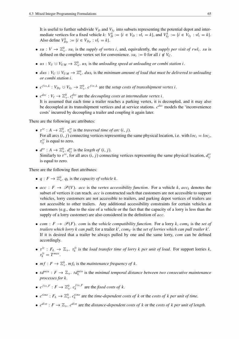
4.3 Mixed Integer Programming Formulations 65
It is useful to further subdivide VD and VIT into subsets representing the potential depot and inter-mediate vertices for a fixed vehicle k: V k
D := {i ∈ VD : vli = k}, and V kIT
:= {i ∈ VIT : vli = k}.Also define V k
DP:= {i ∈ VDP : vli = k}.
• su : V → Z0+
. sui is the supply of vertex i , and, equivalently, the supply per visit of rwli . su isdefined on the complete vertex set for convenience. sui := 0 for all i 6∈ VC .
• us : VU ·∪ VU M → Z0+
. usi is the unloading speed at unloading or combi station i .
• dus : VU ·∪ VU M → Z0+
. dusi is the minimum amount of load that must be delivered to unloadingor combi station i .
• c f i x,L : VDT·∪ VIT → Z0
+. c f i x,L are the setup costs of transshipment vertex i .
• cdec : VI → Z0+
. cdeci are the decoupling costs at intermediate vertex i .
It is assumed that each time a trailer reaches a parking vertex, it is decoupled, and it may alsobe decoupled at its transshipment vertices and at service stations. cdec models the ‘inconveniencecosts’ incurred by decoupling a trailer and coupling it again later.
There are the following arc attributes:
• τ tr : A→ Z0+
. τ tri j is the traversal time of arc (i, j).
For all arcs (i, j) connecting vertices representing the same physical location, i.e. with loci = locj ,τ tr
i j is equal to zero.
• d tr : A→ Z0+
. d tri j is the length of (i, j).
Similarly to τ tr , for all arcs (i, j) connecting vertices representing the same physical location, d tri j
is equal to zero.
There are the following fleet attributes:
• q : F → Z0+
. qk is the capacity of vehicle k.
• acc : F → P(V ). acc is the vertex accessibility function. For a vehicle k, acck denotes thesubset of vertices it can reach. acc is constructed such that customers are not accessible to supportvehicles, lorry customers are not accessible to trailers, and parking depot vertices of trailers arenot accessible to other trailers. Any additional accessibility constraints for certain vehicles atcustomers (e.g., due to the size of a vehicle or the fact that the capacity of a lorry is less than thesupply of a lorry customer) are also considered in the definition of acc.
• com : F → P(F). com is the vehicle compatibility function. For a lorry k, comk is the set oftrailers which lorry k can pull; for a trailer k ′, comk′ is the set of lorries which can pull trailer k ′.If it is desired that a trailer be always pulled by one and the same lorry, com can be definedaccordingly.
• τ lt : FL → Z+. τ ltk is the load transfer time of lorry k per unit of load. For support lorries k,
τ ltk = T max .
• m f : F → Z0+
. m fk is the maintenance frequency of k.
• tdmin : F → Z+. tdmink is the minimal temporal distance between two consecutive maintenance
processes for k.
• c f i x,F : F → Z0+
. c f i x,Fk are the fixed costs of k.
• ctime : FL → Z0+
. ctimek are the time-dependent costs of k or the costs of k per unit of time.
• cdist : F → Z+. cdist are the distance-dependent costs of k or the costs of k per unit of length.

4.3 Mixed Integer Programming Formulations 66
The idea behind the last three attributes is that c f i x,F indicates the costs of making a vehicle availableduring the planning horizon, whereas ctime represents the costs determined by the temporal length ofuse during the planning horizon, and cdist models the costs that depend on the spacial length of eachvehicle’s itinerary.
There is the following composite attribute:
• τm : F × VU M ·∪ VM → Z+. τmki is the maintenance time of k at combi or maintenance station i ,
i.e., the temporal duration of a maintenance process.
Some remarks are appropriate:
A trailer must normally be pulled by some compatible lorry when traversing an arc, but there are twonotable exceptions:
(i) A very tricky aspect of transshipment locations is the following: A load transfer to a trailer at oneof these locations is only possible during a service time window. However, the trailer may parkat such a location before and after the service time window. This means that the lorry pullingthe trailer to and the lorry pulling the trailer away from such a location may reach the locationbefore, respectively, after the service time window. For the corresponding vertices, this impliesthat the trailer and the lorry pulling it may reach such vertices before the opening and after theclosing time. Therefore, in the model, a trailer being pulled to a transshipment location beforethis location’s service time window (this can be sensible because the lorry pulling the trailer maybe needed for something else afterwards) is parked at the respective parking vertex and moves tothe transshipment vertex independently when the service time begins (and a load transfer is to beperformed). If the trailer is coupled at a transshipment location after the service time window,in the model it moves to the respective parking vertex at the end of the service time window.Arcs connecting vertices with disjoint time windows cannot be traversed by a single trailer. Thus,it is clear which parking vertex will be used by the model for correctly routing a trailer. Fortransshipment depot vertices, if a load transfer is performed, this implies that the receiving traileris assigned to the respective depot and must leave the vertex anyway. Hence, if the trailer is tobe coupled after the closing time, it leaves the transshipment depot vertex for the correspondingparking vertex.
(ii) For depot vertices, it is assumed that a vehicle vli may return to its assigned depot vertex i at anytime, even after twbi . This implies that the lorry k pulling a trailer vli back to its assigned depotvertex i must be allowed to enter i after twbi , too. This problem is circumvented by allowingtrailers vli to traverse arcs (h, i) leading from a parking intermediate vertex h with loch = loci tovli ’s assigned depot vertex i without being pulled by a lorry. It must then be ensured that, for eachphysical location for which a depot vertex is created, there is also a parking vertex with a closingtime of T max .
In essence, trailers k ′ are allowed to traverse arcs (h, i) and (i, j) for i ∈ V k′IT
, h, j ∈ VIP withrwli = rwlh = rwlj and arcs (h, i) for h ∈ VIP , i ∈ V k′
D , rwlh = rwli without being pulled by alorry. The set of such arcs for a trailer k ′ is Asingle
k′ .
One little problem that remains is the following. Simultaneous load transfer of two different vehiclesto a lorry and its attached trailer at the same physical transshipment location is possible: One vehicletransfers load to the lorry, the other vehicle transfers load to the trailer. It is not necessary to decouple thetrailer from the lorry in this case. In the model, however, this is represented by the lorry decoupling thetrailer at the latter’s corresponding transshipment vertex, moving singly to its own transshipment vertex,and re-coupling the trailer again afterwards, incurring decoupling costs. This is a minor defect and notworth further modelling efforts.

4.3 Mixed Integer Programming Formulations 67
‘Congestion’ at depots or intermediate locations, i.e., the possibility of having too many vehicles at aphysical location at the same time, is not considered. However, congestion is modelled as far as loadtransfer and unloading processes are concerned.
The issue of a maximum tour duration is not considered in the formulation presented subsequently. Thisformulation allows multiple use of vehicles, i.e., the possibility of a vehicle unloading at a depot andstarting a new tour. The planning horizon is typically one or two days (24 or 48 hours), which meansthat it is too long for one driver to drive a vehicle during the complete planning horizon. Nevertheless,the planning horizon limits the time en route of a vehicle. This means that there must be a change ofdriver at some point in time. In practice, such a change occurs in accordance with legal working timeregulations. It has no effect on the costs of a tour.
4.3.2 A Formulation for the Complete Problem Based on Turn Variables
4.3.2.1 Assumptions
There are two fundamental assumptions in the formulation presented in this section:
(i) The first assumption is that there is a transshipment vertex for each combination of (pertinent)physical location, time window, and vehicle, and that each vehicle visits each of its transshipmentvertices at most once. To see why this is a good idea, consider the possible alternatives:
• If there are as many transshipment vertices as there are combinations of location, time win-dow, and passive vehicle, allowing that each transshipment vertex be visited by any trailer(but at most one) requires introducing many additional variables (compared to the subsequentformulation), namely, variables modelling vehicle movements to and from all transshipmentvertices i are necessary for vehicles k 6= vli .
• Having one transshipment vertex for each time window of each physical location means thateach transshipment vertex may have more than one passive vehicle. It is then difficult to sayto which passive vehicle an active vehicle transfers its load.
If it is considered too restrictive an assumption that each vehicle visits each of its transshipmentvertices at most once during each of the respective location’s time windows, duplicates of therelevant vertices can be introduced.
(ii) The second assumption is that every arc is traversed by each vehicle at most once. The significanceof this postulate is discussed in Section 4.3.5. If a vehicle shall be allowed to travel from vertex ito vertex j more than once, parallel arcs can be introduced. D is assumed to be simple only forsimplicity.
4.3.2.2 Variables
The concepts of turns and of turn variables have been introduced in the previous chapter. The networksused in this chapter are simple, so the notation for turns can be simplified: In a simple digraph, a turn isuniquely described by an ordered sequence of three vertices. If a vehicle traverses an arc (i, j) immedi-ately after an arc (h, i), it performs a turn t in vertex i , and this turn is denoted t = (h, i, j). As before,T is used to denote the set of turns in D.
The formulation uses the following variables:
• xkhi j ∈ {0, 1} ∀ k ∈ F, (h, i), (i, j) ∈ A.
xkhi j =
{1, vehicle k traverses arc (i, j) immediately after arc (h, i)0, otherwise
The xkhi j are the turn variables.

4.3 Mixed Integer Programming Formulations 68
• xk∈ {0, 1} ∀ k ∈ F .
xk=
{1, vehicle k is used0, otherwise
• xkk′i j ∈ {0, 1} ∀ k ∈ FL , k ′ ∈ comk, (i, j) ∈ A.
xkk′i j =
{1, lorry k pulls trailer k ′ over arc (i, j)0, otherwise
The xkk′i j are called lorry-trailer arc variables.
• xdec,k′hi ∈ {0, 1} ∀ k ′ ∈ FT , i ∈ {i ′ ∈ VIT : k ′ = vli ′} ·∪ VS, (h, i) ∈ A.
xdec,k′hi =
{1, trailer k ′ is decoupled at vertex i after traversing arc (h, i)0, otherwise
• yk,mhi ∈ {0, 1} ∀ k ∈ F, m = 1, . . . , m fk, i ∈ VU M ·∪ VM , (h, i) ∈ A.
yk,mhi =
{1, vehicle k undergoes its mth maintenance at vertex i coming from vertex h0, otherwise
• lkhi ∈ R0
+∀ k ∈ F, (h, i) ∈ A.
The amount of load vehicle k is carrying immediately after traversing arc (h, i).
• tkhi ∈ R0
+∀ k ∈ F, (h, i) ∈ A.
The point in time when vehicle k begins its service at vertex i after traversing arc (h, i).
• t lt,k′hi ∈ Z+ ∀ i ∈ VDT
·∪ VIT , vli 6= k ′ ∈ FT , (h, i) ∈ A.The load transfer time of trailer k ′ at transshipment vertex i , after k ′ has reached i via arc (h, i).There is exactly one lorry k that has pulled k ′ to i via (h, i). By the xkk′
hi variables, k then determinesthe load transfer time of k ′ at i .
• tk,m∈ R0
+∀ k ∈ F, m = 1, . . . , m fk .
The point in time when the mth maintenance of k begins.
• td,ki j ∈ R0
+∀ k ∈ F, (i, j) ∈ A.
The point in time when vehicle k departs from vertex i heading for vertex j .
• zk+hi ∈ R0
+∀ k ∈ F, i ∈ VDT
·∪ VIT·∪ VU ·∪ VU M , (h, i) ∈ A.
For i ∈ VDT·∪ VIT , the amount of load transferred from vehicle k to vehicle vli at vertex i after
vehicle k has reached i via arc (h, i).For i ∈ VU ·∪ VU M , the amount of load unloaded from vehicle k at service station i after vehicle khas reached i via arc (h, i).
• zk−hi ∈ R0
+∀ k ∈ F, i ∈ VDT
·∪ VIT·∪ VU ·∪ VU M , (h, i) ∈ A.
For i ∈ VDT·∪ VIT , the amount of load transferred from vehicle vli to vehicle k at vertex i after
vehicle k has reached i via arc (h, i).For i ∈ VU ·∪ VU M , the amount of load collected by vehicle k at service station i after vehicle khas reached i via arc (h, i).These variables model the possibility of a load transfer from a support lorry or a trailer to a collec-tion lorry or a trailer currently pulled by a collection lorry as well as the possibility of transportsbetween unloading and combi stations.
• zi ∈ R0+∀ i ∈ VCLT .
The amount of load transferred at trailer customer i . One index is sufficient here because at mostone lorry and one trailer visit such a vertex.
All turn variables xkhi j and all lorry-trailer arc variables xkk′
i j where h, i , or j are not accessible to thevehicles k and k ′ are equal to zero. Hence, these variables are not necessary; they were defined only forconvenience.
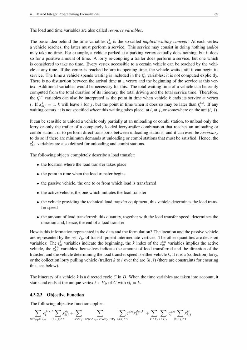
4.3 Mixed Integer Programming Formulations 69
The load and time variables are also called resource variables.
The basic idea behind the time variables tkhi is the so-called implicit waiting concept: At each vertex
a vehicle reaches, the latter must perform a service. This service may consist in doing nothing and/ormay take no time. For example, a vehicle parked at a parking vertex actually does nothing, but it doesso for a positive amount of time. A lorry re-coupling a trailer does perform a service, but one whichis considered to take no time. Every vertex accessible to a certain vehicle can be reached by the vehi-cle at any time. If the vertex is reached before its opening time, the vehicle waits until it can begin itsservice. The time a vehicle spends waiting is included in the tk
hi variables; it is not computed explicitly.There is no distinction between the arrival time at a vertex and the beginning of the service at this ver-tex. Additional variables would be necessary for this. The total waiting time of a vehicle can be easilycomputed from the total duration of its itinerary, the total driving and the total service time. Therefore,the td,k
i j variables can also be interpreted as the point in time when vehicle k ends its service at vertexi . If xk
hi j = 1, k will leave i for j , but the point in time when it does so may be later than td,ki j . If any
waiting occurs, it is not specified where this waiting takes place: at i , at j , or somewhere on the arc (i, j).
It can be sensible to unload a vehicle only partially at an unloading or combi station, to unload only thelorry or only the trailer of a completely loaded lorry-trailer combination that reaches an unloading orcombi station, or to perform direct transports between unloading stations, and it can even be necessaryto do so if there are minimum demands at unloading or combi stations that must be satisfied. Hence, thezk±
hi variables are also defined for unloading and combi stations.
The following objects completely describe a load transfer:
• the location where the load transfer takes place
• the point in time when the load transfer begins
• the passive vehicle, the one to or from which load is transferred
• the active vehicle, the one which initiates the load transfer
• the vehicle providing the technical load transfer equipment; this vehicle determines the load trans-fer speed
• the amount of load transferred; this quantity, together with the load transfer speed, determines theduration and, hence, the end of a load transfer
How is this information represented in the data and the formulation? The location and the passive vehicleare represented by the set VIT of transshipment intermediate vertices. The other quantities are decisionvariables: The tk
hi variables indicate the beginning, the k index of the zk±hi variables implies the active
vehicle, the zk±hi variables themselves indicate the amount of load transferred and the direction of the
transfer, and the vehicle determining the load transfer speed is either vehicle k, if it is a (collection) lorry,or the collection lorry pulling vehicle (trailer) k to i over the arc (h, i) (there are constraints for ensuringthis, see below).
The itinerary of a vehicle k is a directed cycle C in D. When the time variables are taken into account, itstarts and ends at the unique vertex i ∈ VD of C with vli = k.
4.3.2.3 Objective Function
The following objective function applies:∑i∈VDT
·∪VIT
c f i x,Li
∑(h,i, j)∈T
xvlihi j +
∑k′∈FT
∑i∈{i ′∈VIT :k′=vli ′ } ·∪VS
∑(h,i)∈A
cdeci xdec,k′
hi +
∑k′∈FT
∑i∈VIP
cdeci
∑(h,i, j)∈T
xk′hi j

4.3 Mixed Integer Programming Formulations 70
+
∑k∈F
c f i x,Fk xk
+
∑k∈F
∑(i, j)∈A
d tri j cdist
k
∑(h,i, j)∈T
xkhi j +
∑k∈FL
∑i∈V k
D
∑(h,i)∈A
tkhi −
∑(i, j)∈A
td,ki j
ctimek → min (4.1)
The first line of the objective function contains the location-dependent costs, the second line contains thevehicle-dependent costs.
The last summand in the above term deserves explanation. The total ‘working time’ of a lorry is whatis relevant for the time-dependent costs. This total time is not necessarily equal to the value of the tk
hivariable for the arc (h, i) via which the lorry returns to its assigned depot vertex i , because the lorry mayhave started its itinerary later than time zero. (It will not start earlier than necessary precisely because ofthe time-dependent costs, which make it desirable to minimize the total time en route.) The factor to theleft of ctime
k takes this into account.
4.3.2.4 Constraints
The following constraints apply:
Each vehicle must be present to be used, and it must be assigned to exactly one depot:∑{i∈VD :vli=k}
∑(h,i, j)∈T
xkhi j 5 xk
∀ k ∈ F (4.2)
Flow conservation:∑(h,i, j)∈T
xkhi j −
∑(i, j, j ′)∈T
xki j j ′ = 0 ∀ k ∈ F, (i, j) ∈ A (4.3)
Only if the vehicle vli leaves the potential depot vertex i can another vehicle enter i :
xkhi j 5
∑(h′,i, j ′)∈T
xvlih′i j ′ ∀ k ∈ F, i ∈ VD, (h, i, j) ∈ T (4.4)
Each vehicle uses each of its transshipment vertices at most once:∑(h,i, j)∈T
xvlihi j 5 1 ∀ i ∈ VIT (4.5)
Only if the vehicle vli reaches its transshipment vertex i can another vehicle enter i :
xkhi j 5
∑(h′,i, j ′)∈T
xvlih′i j ′ ∀ k ∈ F, i ∈ VIT , (h, i, j) ∈ T (4.6)
Each customer vertex is visited by at most one lorry:∑k∈FL
∑(h,i, j)∈T
xkhi j 5 1 ∀ i ∈ VC (4.7)
Each customer l is visited exactly v fl times:∑i∈V l
C
∑k∈FL
∑(h,i, j)∈T
xkhi j = v fl ∀ l ∈ RW LC (4.8)
Constraints on the number of visits at customer l in specified subsets of l’s time windows:∑{i∈V l
C :twvi∈S}
∑k∈FL
∑(h,i, j)∈T
xkhi j = n ∀ l ∈ RW LC , (S, n) ∈ v f tw
l (4.9)

4.3 Mixed Integer Programming Formulations 71
Constraints on the minimal time between two visits at a customer:
xkhi j = 1 ∧ x k
h′i ′ j ′ = 1⇒ tkhi + vdmin
l 5 t kh′i ′ ∀ k, k ∈ FL , i, i ′ ∈ VC , loci = loci ′,
twbi < twai ′, (h, i, j), (h′, i ′, j ′) ∈ T ( 4.10)
These constraints are equivalent to (omitting the ‘∀’ section for simplicity)
xkhi j + x k
h′i ′ j ′ = 2⇒ tkhi + vdmin
l 5 t kh′i ′, (4.10a)
which can be linearized as follows:
tkhi + vdmin
l + T max(xkhi j + x k
h′i ′ j ′ − 2) 5 t kh′i ′ . (4.10b)
In standard formulations for VRPs, i.e., formulations using arc variables, subtour elimination constraintsare necessary to include the depot in each vehicle’s tour(s). Are such constraints also needed when usingturn variables? Consider Figure 4.4. If all four vertices must be visited, all four depicted arcs must be tra-versed, and there is exactly one cycle constituting a tour. With arc variables, no subtours arise. With turnvariables, though, it is possible to visit all four vertices when the indicated turns t1, t2, t3 are performed,but this leads to two subtours. However, it is impossible to perform both t2 and t3 if the sum of the traveltimes on the arcs and the service times at the vertices of any cycle is strictly positive. Consequently, ifthis is the case, no subtours are possible and no subtour elimination constraints are necessary. Unfor-tunately, in the formulation considered in this section, there may be cycles with a spacial and temporallength of zero. For example, a lorry k with an attached trailer k ′ might reach a parking vertex i , decouplek ′, go to an unloading station i ′ with loci ′ = loci , couple a trailer k, return to i , decouple k, couple k ′,and leave for somewhere else (cf. Figure 4.4). With the arc attributes τ tr and d tr defined as above, thelorry can perform this cycle in zero time units and travel zero length units. If all three vehicles are empty,the load variables are not affected either.
s
s
s sh i
i ′
j
t1
t2
t3
......................................................................................................................................................... .........................................................................................................................................................
...............................................................................................................................................................
........................
.......................
....................
....................
...................................................................................................................................................................
...................................................................................................................................................................
......................................................................................
......................................................................................
Figure 4.4: Turn subtour
There are three ways to deal with this situation:
(i) One way is to set τ tr and d tr to very small positive values ε for all arcs (i, j) connecting verticesrepresenting the same physical location, i.e., with loci = locj .
(ii) The second way is to leave everything as it is and accept the possibility of turn subtours. Suchsubtours can occur only for cycles with a length of zero, so they do not affect the optimal solutionvalue, and neither do they affect any other variables. The arcs any vehicle traverses remain thesame. Only if a vehicle’s itinerary is to be reconstructed from the values of the xk
hi j variables of asolution must care be taken. The Hierholzer Algorithm (Hierholzer 1873) can be applied in thiscase: For each vehicle, its assigned depot vertex must be found out (which is not difficult), the arcemanating from this vertex used by the vehicle must be traversed, and (the) other arc(s) emanatingfrom the head of the first arc it uses must be traversed in the sequence the time and the turnvariables prescribe. At vertices the vehicle leaves more than once at the same time, subtours mayoccur. Such vertices are marked. If a cycle is generated that does not contain all arcs the vehicleuses according to the xk
hi j variable values, the zero-length subtours starting at marked vertices aresuccessively included in the tour containing the assigned depot vertex.

4.3 Mixed Integer Programming Formulations 72
(iii) The third way is to include subtour elimination constraints for the turns. To do this, it must beobserved that the depot (vertex) for each vehicle is not known in advance; it is determined duringthe solution. Hence, to ensure connectivity of a vehicle’s itinerary, it must be ensured that, for eachsubset of vertices not including the respective assigned depot vertex, if the vehicle performs a turninvolving two vertices of this subset (traverses an arc between two vertices of this subset), then italso performs a turn whose first two vertices belong to this subset and whose third vertex does not(traverses an arc leaving this subset). Constraints to ensure this are very complicated to formulate,so the other two alternatives are clearly superior.
Linking of turn and lorry-trailer arc variables:A trailer k ′ must normally be pulled by some compatible lorry when traversing an arc, with the exceptionof the arcs in Asingle
k′ : ∑(h,i, j)∈T
xk′hi j =
∑k∈comk′
xkk′i j ∀ k ′ ∈ FT , (i, j) ∈ A \ Asingle
k′ (4.11)
∑(h,i, j)∈T
xkhi j =
∑k′∈comk
xkk′i j ∀ k ∈ FL , (i, j) ∈ A (4.12)
Linking of lorry-trailer arc and time variables:
xkk′hi = 1⇒ tk
hi 5 tk′hi ∀ k ′ ∈ FT , k ∈ comk′, (h, i) ∈ A (4.13)
xkk′i j = 1⇒ td,k
i j = td,k′i j ∀ k ′ ∈ FT , k ∈ comk′, (i, j) ∈ A (4.14)
The first implication can be rewritten as
tkhi − (1− xkk′
hi )T max 5 tk′hi . (4.13a)
The second implication can be expressed as
xkk′i j = 1⇒ td,k
i j 5 td,k′i j ∧ td,k
i j = td,k′i j , (4.14a)
or
td,ki j − T max(1− xkk′
i j ) 5 td,k′i j ∧ td,k
i j + T max(1− xkk′i j ) = td,k′
i j . ( 4.14b)
Linking of turn, load, and time variables:
xkhi j = 0⇒ lk
i j = tki j = td,k
i j = 0 ∀ k ∈ F, (h, i, j) ∈ T (4.15)
Decoupling a trailer k ′ is not allowed at depot vertices and transshipment intermediate vertices i withvli 6= k ′:
xk′hi j = 1 ∧ xkk′
hi = 1⇒ xkhi j = 1 ∧ xkk′
i j = 1 ∀ i ∈ VD ·∪ VIT , vli 6= k ′ ∈ FT , k ∈ comk′,
(h, i, j) ∈ T ( 4.16)
xkhi j and xkk′
i j are binary variables. Therefore, the ‘=’ signs to the right of the implication can be replacedby ‘=’, and the constraints are equivalent to
xk′hi j + xkk′
hi − 1 5 xkhi j∧ xk′
hi j + xkk′hi − 1 5 xkk′
i j . (4.16a)
These constraints also make sure that, if there is a load transfer from a trailer k ′ to another vehicle, thelorry k (which is assumed to be a collection lorry, see above) which has pulled k ′ to the respective vertexis present during the load transfer.
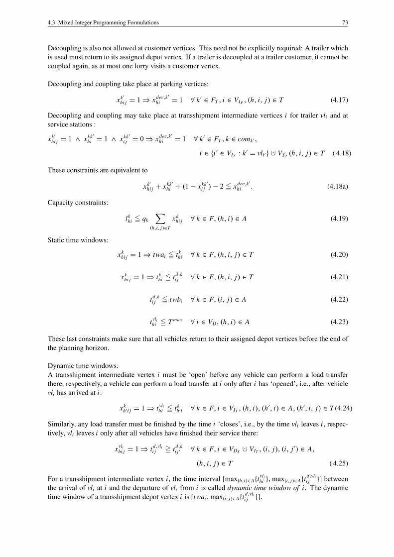
4.3 Mixed Integer Programming Formulations 73
Decoupling is also not allowed at customer vertices. This need not be explicitly required: A trailer whichis used must return to its assigned depot vertex. If a trailer is decoupled at a trailer customer, it cannot becoupled again, as at most one lorry visits a customer vertex.
Decoupling and coupling take place at parking vertices:
xk′hi j = 1⇒ xdec,k′
hi = 1 ∀ k ′ ∈ FT , i ∈ VIP , (h, i, j) ∈ T (4.17)
Decoupling and coupling may take place at transshipment intermediate vertices i for trailer vli and atservice stations :
xk′hi j = 1 ∧ xkk′
hi = 1 ∧ xkk′i j = 0⇒ xdec,k′
hi = 1 ∀ k ′ ∈ FT , k ∈ comk′,
i ∈ {i ′ ∈ VIT : k ′ = vli ′} ·∪ VS, (h, i, j) ∈ T ( 4.18)
These constraints are equivalent to
xk′hi j + xkk′
hi + (1− xkk′i j )− 2 5 xdec,k′
hi . (4.18a)
Capacity constraints:
lkhi 5 qk
∑(h,i, j)∈T
xkhi j ∀ k ∈ F, (h, i) ∈ A (4.19)
Static time windows:
xkhi j = 1⇒ twai 5 tk
hi ∀ k ∈ F, (h, i, j) ∈ T (4.20)
xkhi j = 1⇒ tk
hi 5 td,ki j ∀ k ∈ F, (h, i, j) ∈ T (4.21)
td,ki j 5 twbi ∀ k ∈ F, (i, j) ∈ A (4.22)
tvlihi 5 T max
∀ i ∈ VD, (h, i) ∈ A (4.23)
These last constraints make sure that all vehicles return to their assigned depot vertices before the end ofthe planning horizon.
Dynamic time windows:A transshipment intermediate vertex i must be ‘open’ before any vehicle can perform a load transferthere, respectively, a vehicle can perform a load transfer at i only after i has ‘opened’, i.e., after vehiclevli has arrived at i :
xkh′i j = 1⇒ tvli
hi 5 tkh′i ∀ k ∈ F, i ∈ VIT , (h, i), (h′, i) ∈ A, (h′, i, j) ∈ T (4.24)
Similarly, any load transfer must be finished by the time i ‘closes’, i.e., by the time vli leaves i , respec-tively, vli leaves i only after all vehicles have finished their service there:
xvlihi j = 1⇒ td,vli
i j = td,ki j ′ ∀ k ∈ F, i ∈ VDT
·∪ VIT , (i, j), (i, j ′) ∈ A,
(h, i, j) ∈ T ( 4.25)
For a transshipment intermediate vertex i , the time interval [max(h,i)∈A{tvlihi }, max(i, j)∈A{t
d,vlii j }] between
the arrival of vli at i and the departure of vli from i is called dynamic time window of i . The dynamictime window of a transshipment depot vertex i is [twai , max(i, j)∈A{t
d,vlii j }].
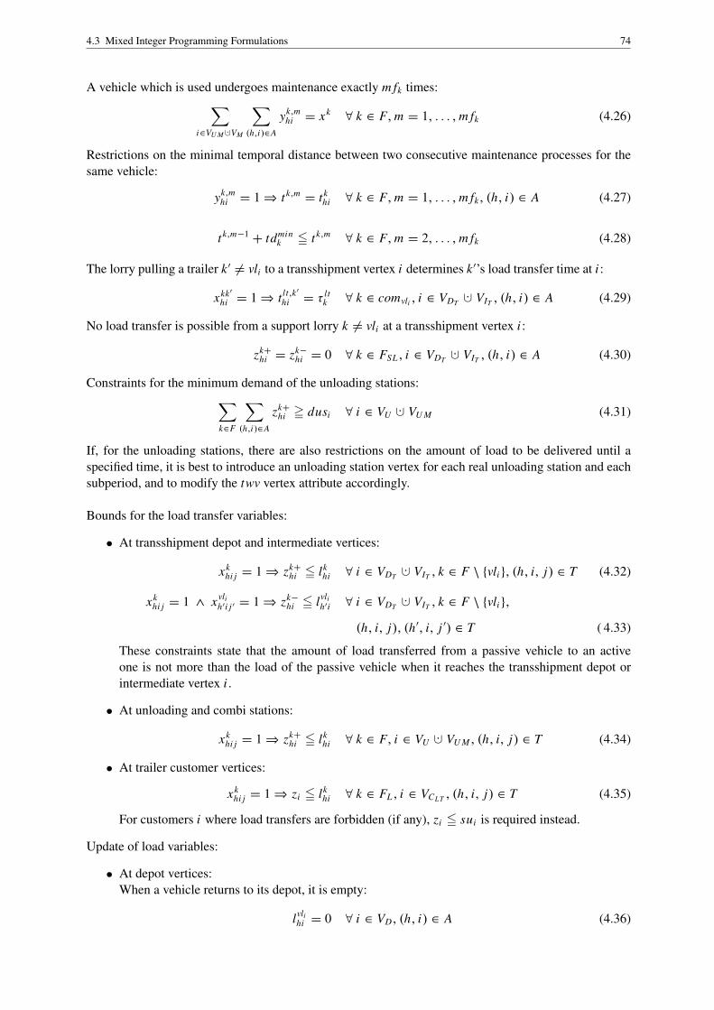
4.3 Mixed Integer Programming Formulations 74
A vehicle which is used undergoes maintenance exactly m fk times:∑i∈VU M ·∪VM
∑(h,i)∈A
yk,mhi = xk
∀ k ∈ F, m = 1, . . . , m fk (4.26)
Restrictions on the minimal temporal distance between two consecutive maintenance processes for thesame vehicle:
yk,mhi = 1⇒ tk,m
= tkhi ∀ k ∈ F, m = 1, . . . , m fk, (h, i) ∈ A (4.27)
tk,m−1+ tdmin
k 5 tk,m∀ k ∈ F, m = 2, . . . , m fk (4.28)
The lorry pulling a trailer k ′ 6= vli to a transshipment vertex i determines k ′’s load transfer time at i :
xkk′hi = 1⇒ t lt,k′
hi = τ ltk ∀ k ∈ comvli , i ∈ VDT
·∪ VIT , (h, i) ∈ A (4.29)
No load transfer is possible from a support lorry k 6= vli at a transshipment vertex i :
zk+hi = zk−
hi = 0 ∀ k ∈ FSL , i ∈ VDT·∪ VIT , (h, i) ∈ A (4.30)
Constraints for the minimum demand of the unloading stations:∑k∈F
∑(h,i)∈A
zk+hi = dusi ∀ i ∈ VU ·∪ VU M (4.31)
If, for the unloading stations, there are also restrictions on the amount of load to be delivered until aspecified time, it is best to introduce an unloading station vertex for each real unloading station and eachsubperiod, and to modify the twv vertex attribute accordingly.
Bounds for the load transfer variables:
• At transshipment depot and intermediate vertices:
xkhi j = 1⇒ zk+
hi 5 lkhi ∀ i ∈ VDT
·∪ VIT , k ∈ F \ {vli }, (h, i, j) ∈ T (4.32)
xkhi j = 1 ∧ xvli
h′i j ′ = 1⇒ zk−hi 5 lvli
h′i ∀ i ∈ VDT·∪ VIT , k ∈ F \ {vli },
(h, i, j), (h′, i, j ′) ∈ T ( 4.33)
These constraints state that the amount of load transferred from a passive vehicle to an activeone is not more than the load of the passive vehicle when it reaches the transshipment depot orintermediate vertex i .
• At unloading and combi stations:
xkhi j = 1⇒ zk+
hi 5 lkhi ∀ k ∈ F, i ∈ VU ·∪ VU M , (h, i, j) ∈ T (4.34)
• At trailer customer vertices:
xkhi j = 1⇒ zi 5 lk
hi ∀ k ∈ FL , i ∈ VCLT , (h, i, j) ∈ T (4.35)
For customers i where load transfers are forbidden (if any), zi 5 sui is required instead.
Update of load variables:
• At depot vertices:When a vehicle returns to its depot, it is empty:
lvlihi = 0 ∀ i ∈ VD, (h, i) ∈ A (4.36)

4.3 Mixed Integer Programming Formulations 75
When a vehicle starts from a parking depot vertex, it is empty:
lvlii j = 0 ∀ i ∈ VDP , (i, j) ∈ A (4.37)
When it starts from a transshipment depot vertex:
xvlihi j = 1⇒ lvli
i j =∑
k∈F\{vli }
∑(h,i)∈A
(zk+hi − zk−
hi )
∀ i ∈ VDT , (h, i, j) ∈ T (4.38)
Vehicles k at transshipment depot vertex i with k 6= vli :
xkhi j = 1⇒ lk
hi − zk+hi + zk−
hi = lki j ∀ i ∈ VDT , k ∈ F \ {vli }, (h, i, j) ∈ T (4.39)
• At parking intermediate vertices:
xkhi j = 1⇒ lk
hi = lki j ∀ k ∈ F, i ∈ VIP , (h, i, j) ∈ T (4.40)
• At transshipment intermediate vertices:
xvlihi j = 1⇒ lvli
hi +∑k∈F
∑(h′,i)∈A
(zk+h′i − zk−
h′i ) = lvlii j
∀ i ∈ VIT , (h, i, j) ∈ T (4.41)
xkhi j = 1⇒ lk
hi − zk+hi + zk−
hi = lki j ∀ k ∈ F \ {vli }, i ∈ VIT , (h, i, j) ∈ T (4.42)
• At lorry customers:
xkhi j = 1⇒ lk
hi + sui = lki j ∀ k ∈ FL , i ∈ VCL , (h, i, j) ∈ T (4.43)
Independent of the acc fleet attribute, these constraints additionally model the possibility that acustomer cannot be served by a lorry because the lorry’s capacity may be less than the customer’ssupply.
• At trailer customers:
– Lorries:
xkhi j = 1⇒ lk
hi + sui − zi = lki j ∀ k ∈ FL , i ∈ VCLT , (h, i, j) ∈ T (4.44)
– Trailers:
xk′hi j = 1⇒ lk′
hi + zi = lk′i j ∀ k ′ ∈ FT , i ∈ VCLT , (h, i, j) ∈ T (4.45)
• At unloading and combi stations:
xkhi j = 1⇒ lk
hi − zk+hi + zk−
hi = lki j ∀ k ∈ F, i ∈ VU ·∪ VU M , (h, i, j) ∈ T (4.46)
It is assumed that there is always enough supply at unloading and combi stations for a vehicle toincrease its load there, in spite of the above constraints for the minimum demand of unloading andcombi stations.
• At combi stations:A vehicle is empty when it undergoes maintenance:
yk,mhi = 1⇒ zk+
hi = lkhi ∀ k ∈ F, m = 1, . . . , m fk, i ∈ VU M , (h, i) ∈ A (4.47)

4.3 Mixed Integer Programming Formulations 76
• At maintenance stations:
xkhi j = 1⇒ lk
hi = lki j ∀ k ∈ F, i ∈ VM , (h, i, j) ∈ T (4.48)
A vehicle is empty when it undergoes maintenance:
yk,mhi = 1⇒ lk
hi = 0 ∀ k ∈ F, m = 1, . . . , m fk, i ∈ VM , (h, i) ∈ A (4.49)
Note that the load constraints are formulated as equality constraints. This accurately models reality.Given a solution to an instance, the information given by these variables can be used directly. On theother hand, it is sometimes preferable to use inequality instead of equality constraints, depending on thesolution method. The load update constraints can also be formulated as inequalities. For example, theload of a vehicle after leaving a parking location is, in reality, exactly equal to the load at the moment ofarrival. But it is logically sufficient to require the load to be no smaller. It will not be any larger (exceptif there is slack) because of the objective function.
Update of time variables:The timing constraints are inequalities because of the implicit waiting concept.
For each depot vertex i , the point in time when vehicle vli departs from it must not be later than the pointin time when vli returns there:
xvlihi j = 1⇒ tvli
hi = td,vlii j ∀ i ∈ VD, (h, i, j) ∈ T (4.50)
For every vehicle and every arc it traverses, the departure time of the vehicle at the tail of the arc plus thetravel time along the arc is less than or equal to the beginning of the service of the vehicle at the head ofthe arc:
xkhi j = 1⇒ td,k
hi + τ trhi 5 tk
hi ∀ k ∈ F, i ∈ V k\ VD, (h, i, j) ∈ T (4.51)
The beginning of the service of a vehicle at a vertex plus the time the service takes is less than or equalto the departure time of the vehicle at that vertex:
xkhi j = 1⇒ tk
hi + t s,khi 5 td,k
i j ∀ k ∈ F, i ∈ V k\ VD, (h, i, j) ∈ T (4.52)
t s,khi is not a variable, it is just a placeholder for the service time of vehicle k at vertex i after k has reached
i via the arc (h, i). At the different vertex types, it is defined as follows:
• At parking depot vertices:
t s,khi = 0 ∀ vli 6= k ∈ FL ( 4.52a)
The above constraints are not applicable for vehicle vli and for trailers.
• At parking intermediate vertices:
t s,khi = 0 ∀ k ∈ F ( 4.52b)
• At transshipment vertices:
t s,vlihi = 0 ( 4.52c)
t s,khi = (zk+
hi + zk−hi )τ lt
k ∀ vli 6= k ∈ FL ( 4.52d)
t s,k′hi = (zk′+
hi + zk′−hi )t lt,k′
hi ∀ vli 6= k ′ ∈ FT ( 4.52e)
The service time is equal to zero for vehicle vli , because vli is the passive vehicle in a load transferat i , and its service time is determined by the active vehicles that perform the load transfer.

4.3 Mixed Integer Programming Formulations 77
• At lorry customers:
t s,khi = suiτ
ltk ∀ k ∈ FL ( 4.52f)
• At trailer customers:
t s,khi = max{suiτ
ltk , ziτ
ltk } ∀ k ∈ FL , ( 4.52g)
i.e., for each k ∈ FL , one constraint is necessary with t s,khi = suiτ
ltk , and one is necessary with
t s,khi = ziτ
ltk . As stated above, at a trailer customer, a load transfer can be performed from lorry to
trailer. The service time therefore depends on sui , if the amount of load transferred is less than orequal to sui ; otherwise, it depends on zi .
t s,k′hi = ziτ
ltk ∀ k ′ ∈ FT ( 4.52h)
For a trailer, the service time at a customer vertex does not really matter; arrival and departure atcustomers are determined by the pulling lorry. So, the service time can be set to zero as well.
• At unloading stations:
t s,khi = (zk+
hi + zk−hi )usi ∀ k ∈ F ( 4.52i)
• At maintenance stations:
t s,khi = yk
hiτmki ∀ k ∈ F ( 4.52j)
• At combi stations:
t s,khi = (zk+
hi + zk−hi )usi + yk
hiτmki ∀ k ∈ F ( 4.52k)
Scheduling/synchronization constraints at transshipment vertices:At any point in time, at most one vehicle can transfer load to another vehicle. This means that if, forexample, a lorry k arrives at a (currently open) transshipment vertex i at time t and wants to transfer anamount of load that will take 10 units of time to transfer, and if another lorry k arrives 5 units of timeafter lorry k, lorry k must wait 5 units of time until it can transfer load.
Such relationships are covered by the concept of implicit waiting, i.e., by the (meaning of the) tkhi vari-
ables. With these variables, it must be forced that the beginning of a load transfer from a vehicle k toanother vehicle vli at transshipment vertex i plus the load transfer time do not overlap with the beginningof a third vehicle’s load transfer, i.e.
tkhi + τ lt
k (zk+hi + zk−
hi ) 5 t khi ∨ t k
hi + τ ltk (z k+
hi+ z k−
hi) 5 tk
hi
∀ k, k ∈ FL , k 6= k, k, k 6= vli , i ∈ VDT·∪ VIT ,
(h, i), (h, i) ∈ A (4.53)
If one of the vehicles that want to transfer load is a trailer, the load transfer time constant in the aboveconstraints must be replaced by the respective load transfer time variable.
The constraints stated as yet do not exclude the possibility that an arc may be traversed by two or moredifferent lorries (though never more than once by the same lorry or trailer). This poses no problem. Inthe above constraints, however, h 6= h must not be required therefore.
The above constraints are disjunctive constraints. They are rewritten as follows (cf. Williams 1999, p.169 ff.). For each ‘5’-constraint, a binary indicator variable δ is introduced which is equal to one if andonly if the associated constraint holds:
tkhi + τ lt
k (zk+hi + zk−
hi )+ T maxδikhkh 5 T max
+ t khi (4.53a)

4.3 Mixed Integer Programming Formulations 78
Then, for each of the above disjunctions,
δikhkh + δi
khkh = 1 (4.53b)
is required.
Scheduling/synchronization constraints for service stations:They are modelled similarly to those for transshipment vertices. The start time of a vehicle’s service at aservice station plus the service time must not overlap with another vehicle’s start time there:
tkhi + t s,k
hi 5 t khi ∨ t k
hi + t s,khi
5 tkhi ∀ k, k ∈ F, k 6= k, i ∈ VS, (h, i), (h, i) ∈ A (4.54)
Here, too, a binary indicator variable δ is introduced.
Parallel maintenance of a lorry-trailer combination is incorporated in the formulation as follows. For acombi station, an additional vertex for the maintenance part of the station is introduced; this vertex hasonly one predecessor and one successor, namely, the corresponding unloading vertex of the station. Thecorresponding arcs have a length and a travel time of zero and can be traversed by single trailers. Then,decoupling at ‘maintenance part’ vertices is forbidden, and the previous constraints are relaxed for therelevant lorry-trailer combinations.
The meta time windows can be modelled as follows. Let the number of meta time windows be mmeta . Thecustomer vertices are grouped into mmeta groups VCm , for m = 1, . . . , mmeta , according to their time win-dows. All arcs and respective variables between customer vertices of different groups can be deleted. Foreach real-world location l where a depot is situated and for each meta time window m = 1, . . . , mmeta
−1,a vertex vlm with a time window starting at the end of m and ending at the beginning of m + 1 is intro-duced. All depot vertices close before the end of the first meta time window.
Then,
yk,mhi = 1⇒ tk
hi = tkh′i ′ ∀ k ∈ F, m = 1, . . . , mmeta, i ∈ VU M ·∪ VM ,
i ′ ∈ VCm , (h, i), (h′, i ′) ∈ A ( 4.55)
is required for the maintenance operations, and
xkhi j = 1⇒
∑(h,vlm , j)∈T
xkhvlm j = 1 ∀ k ∈ F, l ∈ RW L , i ∈ V k
D with loci = l,
(h, i, j) ∈ T, m = 1, . . . , mmeta ( 4.56)
is needed to guarantee that a vehicle returns to the real-world location of its assigned depot vertex be-tween each meta time window.
4.3.2.5 Connection Between Turn Variables and Arc Variables
Single vehicle arc variables xki j with
xki j ∈ {0, 1} ∀ k ∈ F, (i, j) ∈ A,
xki j =
{1, vehicle k traverses arc (i, j)0, otherwise
could easily be introduced in the above formulation by the following constraints:
xkhi −
∑(i, j)∈A
xkhi j = 0 ∀ k ∈ F, (h, i) ∈ A (4.57)
and

4.3 Mixed Integer Programming Formulations 79
xki j −
∑(h,i)∈A
xkhi j = 0 ∀ k ∈ F, (i, j) ∈ A. (4.58)
However, a complete substitution (in all constraints) of the turn variables by an expression containingonly arc variables is not possible. This means that the turn variables are indispensable for the aboveformulation, whereas single vehicle arc variables are not needed.
In essence, the digraph D considered in this section is equivalent to a digraph D′ with one vertex foreach arc of D and one arc for each turn in D. The idea of this transformation is illustrated in Figure 4.5.The above formulation based on turn variables corresponds to an equivalent formulation in D′ based onarc variables. (D′ is the dual network of D, cf. p. 29).
s
s
s sh i
i ′
j......................................................................................................................................................... .........................................................................................................................................................
........................
....................... ...................................................................................................................................................................
...................................................................................................................................................................
.................................................................................... ............
s
s
s
s
i ′i
hi
i i ′
i jhi j
hii ′ i ′i j
i i ′i
i ′i i ′....................................................................................................................................................................................................................................
.............................................................................................................................................................................................................................
..................................................................................................................................................................................................................................................................................................................................................................................................................................................................................................... ......................................
..............................
..............................
..............................
..............................
..............................
..............................
..............................
............................
Figure 4.5: Transformation of a turn-based into an arc-based network
4.3.2.6 Critical Appraisal of the ‘Complete’ Problem
The formulation presented in this section is extremely complicated and cannot be solved exactly. Al-though the problem encompasses quite a lot of detailed technical aspects (which, however, is necessaryfor operative planning), it was not foreseeable that modelling the VRPTT would be so involved. In par-ticular, there is a large number of logical constraints (implications and disjunctions), and the logic ofload transfers between arbitrary vehicles is very intricate. The number of different variable and con-straint types necessary to describe this logic is astonishing. Therefore, sections 4.3.1 and 4.3.2 mainlyserve three purposes:
(i) they provide a detailed and systematic data model and a graph-theoretical representation of thecomplete VRPTT
(ii) they highlight the difficulty of considering trailers and transshipments
(iii) they show that and how turn variables can be used for modelling vehicle routing problems
Considering the intractability of the complete problem, the remainder of this chapter (and the entireChapter 5) strive to answer the following question:
Which aspects of the VRPTT can be considered in a model that can still be solved exactly?
4.3.3 A Formulation for a ‘Core’ Problem Based on Arc Variables
In this section, a ‘core’ VRPTT is considered, which is confined to central aspects of the ‘complete’problem. The notation of section 4.3.1 is used unless otherwise specified.
4.3.3.1 Simplifications
The following simplifications are made in this section:

4.3 Mixed Integer Programming Formulations 80
• All vehicles start from the same fixed depot and return to it at the end of the planning horizon.There are no restrictions on the minimum amount of load to be delivered to the depot until acertain point in time.
• The planning horizon is only one period. This means that maintenance is not considered. It isassumed that a vehicle is maintained after it has returned to the depot. Hence, the time costs formaintenance are not relevant. As in the complete problem above, there are no restrictions on theduration of a tour other than the length of the planning horizon. A potentially necessary change ofdriver is not considered.
• Each customer may have several disjoint time windows, but must be visited exactly once.
• There are no parking locations, there are only transshipment locations with one or more disjointtime windows.
• There is no distinction between visiting and service time windows.
• Meta time windows are not considered.
• Each physical location corresponding to a trailer customer can also be used as a transshipmentlocation.
• There are no unloading or combi stations.
• Load transfer is only possible from a collection lorry to a trailer, and the load transfer time per unitof load is the same for all lorries.
4.3.3.2 Underlying Network
The formulation is based on a time-space-operation-vehicle network D = (V, A). V is comprised asfollows. There is one start depot vertex o and one end depot vertex d , both with a time window of[0, T max ]. For each customer c and each of its time windows, there is one vertex. For each combinationof physical transshipment location (pure transshipment location or trailer customer location), time win-dow, and trailer, there are (at least) two vertices representing the operations decoupling, transshipment,and coupling. To be precise, for each transshipment location l and each trailer k ′, there are nT S
k′l vertices
vdecouplek′l , vtrans f er,1
k′l , . . . , vtrans f er,nT S
k′l−2
k′l , vcouplek′l . Vdecouple is the set of decoupling vertices, Vtrans f er is the
set of transfer vertices, and Vcouple is the set of coupling vertices. V k′decouple is the set of decoupling ver-
tices of trailer k ′, and V k′trans f er and V k′
couple are defined analogously. VIT := Vdecouple ·∪ Vtrans f er ·∪ Vcouple.The idea behind this separation of transshipment locations and processes is the following: A vertexvdecouple
k′l ∈ Vdecouple can only be reached by a lorry pulling the corresponding trailer k ′. The lorry thenleaves the vertex singly, the trailer moves on to vtrans f er,1
k′l , the first pertinent transshipment vertex. Avertex vtrans f er,i
k′l ∈ Vtrans f er can only be reached and left by a single lorry and by the correspondingtrailer k ′ (where the latter comes from the preceding transshipment vertex vtrans f er,i−1
k′l and moves on tothe succeeding transshipment vertex vtrans f er,i+1
k′l ). A vertex vcouplek′l ∈ Vcouple can only be reached by a
single lorry and by the corresponding trailer (where the latter comes from the preceding transshipment
vertex vtrans f er,nT S
k′l−2
k′l ), and be left by a lorry pulling the corresponding trailer.
Lorries can visit all vertices of D, except for decoupling and coupling vertices of incompatible trailersand inaccessible customers (e.g., lorry customers with too much supply for a certain lorry). Trailers canonly visit their corresponding transshipment vertices, trailer customers, and, of course, the start and theend depot vertex.
A contains the following arcs:
• (o, d) (for unused vehicles)
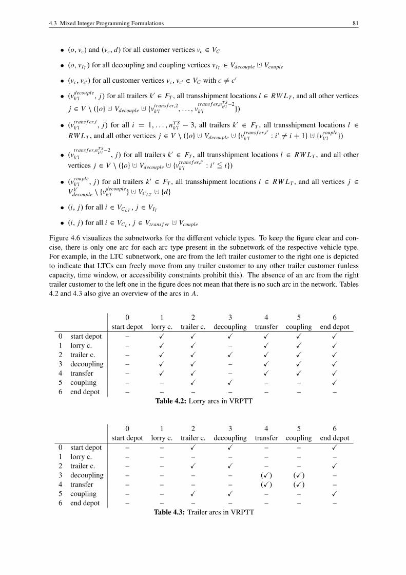
4.3 Mixed Integer Programming Formulations 81
• (o, vc) and (vc, d) for all customer vertices vc ∈ VC
• (o, vIT ) for all decoupling and coupling vertices vIT ∈ Vdecouple ·∪ Vcouple
• (vc, vc′) for all customer vertices vc, vc′ ∈ VC with c 6= c′
• (vdecouplek′l , j) for all trailers k ′ ∈ FT , all transshipment locations l ∈ RW LT , and all other vertices
j ∈ V \ ({o} ·∪ Vdecouple ·∪ {vtrans f er,2k′l , . . . , v
trans f er,nT Sk′l−2
k′l })
• (vtrans f er,ik′l , j) for all i = 1, . . . , nT S
k′l − 3, all trailers k ′ ∈ FT , all transshipment locations l ∈RW LT , and all other vertices j ∈ V \ ({o} ·∪ Vdecouple ·∪ {v
trans f er,i ′
k′l : i ′ 6= i + 1} ·∪ {vcouplek′l })
• (vtrans f er,nT S
k′l−2
k′l , j) for all trailers k ′ ∈ FT , all transshipment locations l ∈ RW LT , and all othervertices j ∈ V \ ({o} ·∪ Vdecouple ·∪ {v
trans f er,i ′
k′l : i ′ 5 i})
• (vcouplek′l , j) for all trailers k ′ ∈ FT , all transshipment locations l ∈ RW LT , and all vertices j ∈
V k′decouple \ {v
decouplek′l } ·∪ VCLT
·∪ {d}
• (i, j) for all i ∈ VCLT , j ∈ VIT
• (i, j) for all i ∈ VCL , j ∈ Vtrans f er ·∪ Vcouple
Figure 4.6 visualizes the subnetworks for the different vehicle types. To keep the figure clear and con-cise, there is only one arc for each arc type present in the subnetwork of the respective vehicle type.For example, in the LTC subnetwork, one arc from the left trailer customer to the right one is depictedto indicate that LTCs can freely move from any trailer customer to any other trailer customer (unlesscapacity, time window, or accessibility constraints prohibit this). The absence of an arc from the righttrailer customer to the left one in the figure does not mean that there is no such arc in the network. Tables4.2 and 4.3 also give an overview of the arcs in A.
0 1 2 3 4 5 6start depot lorry c. trailer c. decoupling transfer coupling end depot
0 start depot – X X X X X X1 lorry c. – X X – X X X2 trailer c. – X X X X X X3 decoupling – X X – X X X4 transfer – X X – X X X5 coupling – – X X – – X6 end depot – – – – – – –
Table 4.2: Lorry arcs in VRPTT
0 1 2 3 4 5 6start depot lorry c. trailer c. decoupling transfer coupling end depot
0 start depot – – X X – – X1 lorry c. – – – – – – –2 trailer c. – – X X – – X3 decoupling – – – – (X) (X) –4 transfer – – – – (X) (X) –5 coupling – – X X – – X6 end depot – – – – – – –
Table 4.3: Trailer arcs in VRPTT

4.3 Mixed Integer Programming Formulations 82
N N
u u
� �
� � �
� � �o d
Lorry customers
Trailer customers
Decouple Trans-fer
Couple ppppppppppppppppppppppppppppppppppppppppppppppppppppppppppppppppppppppppppppppppppppppppppppppppppppppppppppppppppppppppppppppppppppppppppppppppppppppppppppppppppppppppppppppppppppppppppppp pppppppppppppppppppppppppppppppppppppppppppppppppppppppppppppppppppppppppppppppppppppppppppppppppppppppppppppppppppppppppppppppppppppppppppppppppppppppppppppppppppppppppppppppppppppppppppppppppppppppppppppppppppppppppppppp pppppppppppp pppppppppppppppppppppppppppppppppppppppppppppppppppppppppppppppppppppppppppppppppppppppppppppppppppppppppppppppppppppppppppppppppppppppppppppppppppppppppppppppppppppppppppppp pppppppppppp ppppppppppppppppppppppppppppppppppppppppppppppppppppppppppppppppppppppppppppppppppppppppppppppppppppppppppppppppppppppppppppppppppppppppppppppppppppppppppppppppppppppppppppppppppppppppppppppppppppppppppppppp pppppppppppppppppppppppppppppppppppppppppppppppppppppppppppppppppppppp pppppppppppp
pppppppppppppppppppppppppppppppppppppppppppppppppppppppppppppppppppppppppppppppppppppppppppppppppppppppppppppppppppppppppppppppp ppppppppppppppppppppppppppppppppppppppppppppppppppppppppppppppppppppppppppppppppppppppppppppppppppppppppppppppppppppppppppppppppppppppppppppppppppppppppppppppppppppppppppppppppppppppppppppp ppppppppppppN N
� �
� �
� �o d
Lorry customers
Trailer customers
Decouple Couple
Network vertices Subnetwork for lorry-trailer combinations
..............................
..............................
..............................
..............................
..............................
..............................
..............................
..........................
....................................................................................................................................................................................................................... ............
.................................................................................................................................................................................................................................................. ............
................................................................................................................................................................................................................................................................................................. .......................
......................
......................
....................................
..................................
..................................
..................................
......................................................................................................................................................................................................................................................................................................................... ............
............................................................................................. ............................................................................................. ......................
....................
....................
..........................................
............................................................................................. ..................................
......................
..................................
............ ............................................................................ ............
............................................................................... ............
.............................................................................................................................................................................................................................................. ............
...........................................................................
........
........
........
........
........
...................
............
........
........
........
........
........
........
........
..............
...........................................................................
...............
................................................................................................................................................................................................................... ............
......................................
......................................
......................................
......................................
......................................
..........................
........................................................................................................................................................................................................................... ..................
................................................................................................................................................
..................
..................
..................
....
..................................................................................................
.............. ............
.............................
............... ............N N
u u
� �
� � �
� � �o d
Lorry customers
Trailer customers
Decouple Trans-fer
Couple
............. ....................... ............ ............. ....................... ............
............. ....................... ............ ............. ....................... ............
� � �
� � �
Lorry customers
Trailer customers
Decouple Trans-fer
Couple
Subnetwork for single lorries Subnetwork for single trailers
Figure 4.6: VRPTT core problem subnetworks
The arcs (vdecouplek′l , vcouple
k′l ) model the possibility that a lorry can wait for a trailer at a transshipment lo-cation while other lorries perform a load transfer. It is not necessary to introduce arcs (vtrans f er,i
k′l , vcouplek′l )
for i ∈ {1, . . . , nT Sk′l − 3}, as it is not restrictive to require that the last transshipment operation involving
a trailer k ′ at a trailer location l be always performed by the lorry k that will eventually pull k ′ away froml. This is because it is not sensible to allow k to wait at one of the transshipment intermediate vertices ofk ′ at l, because k ′ can be pulled away from l only after all transshipment operations involving k ′ at l havebeen performed.
AL is the set of arcs of D that can be traversed by lorries. Lorries cannot traverse arcs (vdecouplek′l , vtrans f er,1
k′l ),
(vtrans f er,ik′l , vtrans f er,i+1
k′l ), . . . , (vtrans f er,nT S
k′l−2
k′l , vcouplek′l ). The corresponding trailers k ′ can traverse these
arcs, and these arcs, together with the arc (o, d), form the set Asinglek′ .
4.3.3.3 Assumptions
For the formulation presented subsequently, the following two fundamental assumptions are made:
(i) Each vertex is visited by each vehicle at most once.
(ii) Each trailer uses each transshipment location at most once, and each transshipment vertex isreached by at most one lorry.
Thus, for each trailer, there are at most nT Sk′l transshipment operations at each transshipment location,
and it is clear which lorry performs each of these transshipments. This means that, on the one hand,scheduling constraints such as (4.53) in the turn variable formulation are not necessary. On the otherhand, the number of vertices is smaller in the turn variable formulation, in which there is always onlyone vertex for each combination of location, time window, and trailer. As for the ‘correct’ choice of nT S
k′l ,note that, in the worst case, a feasible solution to an instance may exist only when, for each trailer, there

4.3 Mixed Integer Programming Formulations 83
are as many intermediate and coupling vertices as there are lorry customers, because it may be necessaryto perform a load transfer after each visit to a lorry customer. Consequently, an optimal solution obtainedwith the formulation may only be an optimal solution to an underlying problem instance if there are asmany opportunities for a load transfer at the right transshipment location as there are lorry customers.Depending on the instance data, however, better values for nT S can be computed.
4.3.3.4 The Formulation
There are the following variables:
• xki j ∈ {0, 1} ∀ k ∈ F, (i, j) ∈ Ak .
xki j =
{1, vehicle k traverses arc (i, j)0, otherwise
• lki ∈ R0
+∀ k ∈ F, i ∈ V k .
The amount of load vehicle k is carrying when reaching vertex i , before k begins its service at i .
• tki ∈ R0
+∀ k ∈ F, i ∈ V k .
The point in time when vehicle k begins its service at vertex i .
The resulting formulation is:
(VRPTT):∑k∈F
∑(i, j)∈Ak
cki j x
ki j +
∑k∈FL
ctimek (tk
d − tko )→ min (4.59)
subject to∑i∈V l
C
∑k∈FL
∑(h,i)∈Ak
xkhi = 1 ∀ l ∈ RW LC (4.60a)
∑(h,i)∈Avli
xvlihi 5 1 ∀ i ∈ VIT (4.60b)
∑k∈FL
∑(h,i)∈Ak
xkhi −
∑(h′,i)∈Avli
xvlih′i 5 0 ∀ i ∈ VIT (4.60c)
xk′i j −
∑k∈comk′∩{k∈FL :(i, j)∈Ak }
xki j 5 0 ∀ k ′ ∈ FT , (i, j) ∈ Ak′
\ Asinglek′ (4.60d)
xkhi = 1⇒ tk′
i 5 tki ∀ k ′ ∈ FT , i ∈ (VCLT
·∪VIT ) ∩ V k′, k ∈ FL , (h, i) ∈ Ak(4.60e)
xk′hi = 1⇒ tk
i 5 tk′i ∀ k ′ ∈ FT , i ∈ (VCLT
·∪VIT ) ∩ V k′, k ∈ FL , (h, i) ∈ Ak′(4.60f)
xki j = 1 ∧ xk′
i j = 1⇒ lki + lk′
i + sui 5 lkj + lk′
j
∀ i ∈ VCT , k ∈ FL , k ′ ∈ comk, (i, j) ∈ Ak∩ Ak′ (4.60g)
xvlii j = 1 ∧ xk
i j ′ = 1⇒ lvlii + (lk
i − lkj ′) 5 lvli
j ∀ i ∈ Vdecouple, k ∈ comvli , (i, j) ∈ Avli , (i, j ′) ∈ Ak (4.60h)
xvlii j = 1 ∧ xk
i j ′ = 1⇒ lvlii + (lk
i − lkj ′) 5 lvli
j ∀ i ∈ Vtrans f er , k ∈ FL , (i, j) ∈ Avli , (i, j ′) ∈ Ak (4.60i)
xvlii j = 1 ∧ xk
i j = 1⇒ lvlii + (lk
i − lkj ) 5 lvli
j ∀ i ∈ Vcouple, k ∈ comvli , (i, j) ∈ Avli ∩ Ak (4.60j)

4.3 Mixed Integer Programming Formulations 84
∑(i,d)∈Ak
xkid = 1 ∀ k ∈ F (4.61a)
∑(h,i)∈Ak
xkhi −
∑(i, j)∈Ak
xki j = 0 ∀ k ∈ F, i ∈ V k
\ {o, d} (4.61b)
xvlii j = 1⇒ tvli
i + (lvlij − lvli
i )τ lt 5 twbi ∀ i ∈ VIT , (i, j) ∈ Avli (4.61c)
xki j = 1⇒ lk
i + sui 5 lkj ∀ k ∈ FL , i ∈ VCL , (i, j) ∈ Ak (4.61d)
xki j = 1⇒ lk
i 5 lkj ∀ k ∈ F, i ∈ {o} ·∪ VCLT , (i, j) ∈ Ak (4.61e)
xki j = 1⇒ lk
i + sui − 2qk
∑k′∈comk∩{k′∈FT :(i, j)∈Ak′ }
xk′i j 5 lk
j
∀ k ∈ FL , i ∈ VCLT , (i, j) ∈ Ak (4.61f)
xki j = 1⇒ lk
j 5 lki ∀ k ∈ FL , i ∈ VIT , (i, j) ∈ Ak (4.61g)
xvlii j = 1⇒ lvli
i 5 lvlij ∀ i ∈ Vtrans f er , (i, j) ∈ Avli (4.61h)
xkoi = 1⇒ tk
o + τ troi 5 tk
i ∀ k ∈ F, (o, i) ∈ Ak (4.61i)
xki j = 1⇒ tk
i + τ tri j 5 tk
j ∀ k ∈ FL , i ∈ VC , (i, j) ∈ Ak (4.61j)
xki j = 1⇒ tk
i + (lki − lk
j )τlt+ τ tr
i j 5 tkj ∀ k ∈ FL , i ∈ VIT , (i, j) ∈ Ak (4.61k)
xvlii j = 1⇒ tvli
i + (lvlij − lvli
i )τ lt+ τ tr
i j 5 tvlij ∀ i ∈ VIT , (i, j) ∈ Avli (4.61l)
xki j ∈ {0, 1} ∀ k ∈ F, (i, j) ∈ Ak (4.62a)
0 5 lki 5 qk ∀ k ∈ F, i ∈ V k (4.62b)
twai 5 tki 5 twbi ∀ k ∈ F, i ∈ V k (4.62c)
(4.59) is the objective function, which minimizes total costs. The cost coefficient cki j indicates the
distance-dependent costs of vehicle k traversing arc (i, j). For the arcs emanating from the start de-pot vertex (except for the arc (o, d)), the fixed costs for using vehicle k are also contained in ck
i j . It isassumed that all arc costs and arc travel times are strictly positive. However, movements between ver-tices corresponding to the same physical location incur only very small positive costs εc and take onlya very small amount of time εt . tk
o denotes the point in time when vehicle k leaves the start depot. Thismay be later than time zero.
Constraints (4.60) are logically coupling constraints (i.e., constraints involving more than one vehicle).(4.60a)–(4.60d) are the routing synchronization constraints, (4.60e) and (4.60f) are temporal synchro-nization constraints (observance of dynamic time windows), and (4.60g)–(4.60j) are load synchroniza-tion constraints. (4.61) are non-coupling constraints, and (4.62) determine the ranges of the variables.
(4.60a) are the usual customer covering constraints. (4.60b) ensure that each transshipment vertex isvisited at most once by the corresponding trailer. (4.60c) make sure that a transshipment vertex i is onlyvisited by a lorry if the corresponding trailer visits this vertex, and, hence, that at most one lorry visits atransshipment vertex. (4.60a)–(4.60c) imply that each vertex in V \ {o, d} is visited by at most one lorry

4.3 Mixed Integer Programming Formulations 85
and one trailer. (4.60d) guarantee that a trailer k ′ is pulled by a compatible lorry if k ′ traverses a spacialarc. (4.60e) and (4.60f) state that the beginning of the service at a trailer customer or transshipmentvertex is the same for a trailer and a lorry that both visit the vertex. For i ∈ (VCLT
·∪ Vdecouple) ∩ V k′ ,it is sufficient to require these two constraints for k ∈ comk′, (h, i) ∈ Ak′
∩ Ak . Constraints (4.60e)and (4.60f) are similar to the ‘same departure time constraints’ used in aircraft routing and schedulingproblems, cf. Section 4.2. (4.60g)–(4.60j) are the load update constraints for both types of vehicle attrailer customer and transshipment vertices. (4.60g) state that the supply of a trailer customer is dividedup arbitrarily between the lorry and the trailer visiting the customer.
(4.61a) require that each vehicle reach the end depot (possibly via the arc (o, d)). (4.61b) are the flowconservation constraints, and (4.61c) make sure that the static time windows are met. (4.61c) take theservice time at transshipment vertices into account: The load transfer must be finished by the end of thetime window. Note that, because of (4.60e), (4.60f), and (4.60h)–(4.60j), it is sufficient to require (4.61c)for vli . It is assumed that the service time at customer vertices i is included in the traversal times ofthe arcs (i, j). By shifting the original twbi value backwards by the service time, the time windows forcustomer vertices can be adapted such that the collection of the supply is finished by the end of the timewindow.
The next constraints, (4.61d), are the load update constraints for the lorries at lorry customer vertices.Constraints (4.61e) state that, at a trailer customer vertex, the amount of load transferred to the traileris not more than the customer supply. This is a sensible requirement, because, as stated above, for eachtrailer customer location, there is also a set of transshipment vertices, and movements between verticescorresponding to the same physical location incur virtually no costs and take virtually no time. Con-straints (4.61f) are for the correct update of the load variables at trailer customer vertices visited by asingle lorry. Constraints (4.61g) make sure that no load transfer from trailer to lorry is possible, respec-tively, that the amount of load transferred from a lorry to a trailer is non-negative. Without this constraint,negative load transfer times can result. (4.61h) make sure that the load of a trailer does not decrease attransshipment intermediate vertices not visited by a lorry.
Constraints (4.61i)–(4.61l) are the constraints for the update of the time variables: (4.61i) are for the arcsemanating from the start depot, (4.61j) are for lorries on arcs emanating from customer vertices, (4.61k)are for lorries at transshipment vertices, and (4.61l) are for the trailers at their transshipment vertices.
When nT Sk′l = 4, a solution where, for example, a lorry visits vtrans f er,1
k′l after vtrans f er,2k′l for some k ′l
represents the same real-world process as a solution where the lorry visits vtrans f er,2k′l after vtrans f er,1
k′l .Such symmetries with respect to the sequence of transshipment subtours, i.e., of visits of transshipmentintermediate vertices of one real-world location by one and the same lorry (transshipment subtour sym-metries), are avoided in the formulation by constraints (4.61l). However, if two different lorries visittwo transshipment vertices for some k ′l, it does make a difference which lorry visits which vertex: Asolution where lorry k1 visits vertex vtrans f er,i
k′l and lorry k2 visits vtrans f er,i+1k′l is structurally different from
(represents a different real-world process than) a solution where it is the other way round, because thefirst solution implies that lorry k2 can start its transshipment process only after the transshipment processof lorry k1 is finished; in the second solution it is vice versa.
Constraints of the form
tki − T max
∑(h,i)∈Ak
xkhi 5 0 ∀ k ∈ F, i ∈ V k, (4.63)
are not necessary, but may be helpful in an implementation (by ‘guiding’ the solution algorithm).
Formulation (4.59)–(4.62) includes the TTRP as described by Chao 2002 and Scheuerer 2004.

4.3 Mixed Integer Programming Formulations 86
The consideration of support vehicles is trivial. The assumption that a load transfer is only allowed froma collection lorry to a trailer implies that all support lorries can be assumed to have a capacity of zero(which will most often be the case in reality anyway, see the introduction). Hence, it is sufficient not tointroduce any variables for support vehicles on arcs leading to or emanating from customer vertices.
Multiple use of vehicles can be modelled in the network used for the core problem by introducing subpe-riods and additional depot vertices and connecting them to the original vertices, taking into account loadtransfer and driving times. A depot vertex for period t is connected to its neighbouring depot vertices ofperiods t − 1 and t + 1. All vehicles can move in time along the arcs connecting these depot vertices.Thus, a support lorry can park a support trailer somewhere, return to a depot vertex, couple another sup-port trailer, park it elsewhere, re-couple the first support trailer and pull it to a later depot vertex and soon. Similarly, a collection lorry (with or without a trailer) can unload at such a depot vertex and continuecollection afterwards. These additional intermediate depot vertices can be visited by more than one lorryand more than one trailer, but at most once by each vehicle. The formulation for the core problem has tobe modified slightly. In particular, if Vdepot is the set of these additional depot vertices, (4.60e) have tobe supplemented by
xkhi = 1 ∧ xk′
hi = 1⇒ tk′i 5 tk
i ∀ k ′ ∈ FT , h, i ∈ Vdepot , k ∈ comk′, (h, i) ∈ Ak∩ Ak′, (4.64)
(4.60f) need an analogous supplement, and the load and time update at the depot vertices must be
xki j = 1⇒ lk
j 5 0 ∀ k ∈ F, i ∈ Vdepot , (i, j) ∈ Ak, (4.65)
and
xki j = 1⇒ tk
i + lki τ
lt+ τ tr
i j 5 tkj ∀ k ∈ F, i ∈ Vdepot , (i, j) ∈ Ak . (4.66)
A two-period planning horizon can be modelled by an ‘end-of-day-one’ depot vertex. All customer andtransshipment vertices with a time window lying entirely in day one are connected to this vertex, andall customer and transshipment vertices with a time window lying entirely in day two can be reachedonly from this vertex and from other vertices of day two, depending on the respective time windows anddriving times, but not from vertices of day one. Time windows stretching over more than one day lead totwo disjoint time windows, one for each day.
To compute an optimal solution to a real-world VRPTT instance, the above-mentioned extensions mustbe considered. However, although these extensions are important from a practical point of view, they arenot new from a modelling perspective, and the above formulation is still complicated enough withoutthem. Hence, they are not considered in the core problem.
4.3.4 A Formulation for the Core Problem Based on Path Variables
In this section, a reformulation of (4.59)–(4.62) that could be used in a branch-and-price algorithm isdeveloped. The subsequent exposition follows Desaulniers et al. 1998.
The usual decomposition approach for VRPs can also be applied to the VRPTT. The logically couplingconstraints (4.60), i.e., the constraints involving more than one vehicle, define the master program; thenon-coupling constraints (4.61), i.e., the vehicle-specific constraints, define the sub- or pricing problems.Constraints (4.60b) are essentially non-coupling constraints in that each one of them includes only vari-ables concerning one trailer. Nevertheless, it is just as well possible to put them in the master program.
4.3.4.1 The Master Program
The formulation presented in the previous section uses arc variables for each relevant combination oflorry or trailer k and arc (i, j). Branch-and-price approaches for vehicle routing problems use path vari-ables in the master program: There is one variable for each feasible o-d-path of each vehicle. As for

4.3 Mixed Integer Programming Formulations 87
VRPs without trailers, also for the VRPTT, each feasible tour of a vehicle in the network used in theprevious section is an elementary path from the start depot vertex to the end depot vertex through therespective subnetwork. This is true for the lorries as well as for the trailers. In reality, though, the vehicleitineraries will contain cycles starting and ending at transshipment locations.
It follows from the flow decomposition theorem (cf. Ahuja et al. 1993, p. 80 f.) that the extreme pointsof the convex hull of all points fulfilling the pricing problems’ constraints (4.61)–(4.62) correspond topaths from o to d in D, some of which may be non-elementary, because D contains cycles. However,non-elementary paths can never be part of a feasible solution due to the master program constraints.
The pricing problems’ extreme points are described by flow and resource vectors
(xkp, lk
p, tkp) = (xk
i j p, lkip, tk
ip) ∀ k ∈ F, p ∈ Pk, (i, j) ∈ Ak, (4.67)
where Pk is the set of extreme points for vehicle k ∈ F .
Any solution to (4.61)–(4.62) can then be expressed as a convex combination of these extreme points:
xki j =
∑p∈Pk
xki j pλ
kp ∀ k ∈ F, (i, j) ∈ Ak (4.67a)
xki j ∈ {0, 1} ∀ k ∈ F, (i, j) ∈ Ak (4.67b)
lki =
∑p∈Pk
lkipλ
kp ∀ k ∈ F, i ∈ V k (4.67c)
tki =
∑p∈Pk
tkipλ
kp ∀ k ∈ F, i ∈ V k (4.67d)
∑p∈Pk
λkp 5 1 ∀ k ∈ F (4.67e)
λkp = 0 ∀ k ∈ F, p ∈ Pk (4.67f)
In constraints (4.67e), ‘5’ instead of ‘=’ is used. This is possible, if not using a vehicle does not incurany (fixed) costs, as is assumed here. Therefore, the arc (o, d) is not necessary and is removed.
The integer master program (IMP) is then (linearizing all implications in (4.60) by using appropriateconstants):∑k∈F
∑p∈Pk
∑(i, j)∈Ak
cki j x
ki j p
λkp +
∑k∈FL
∑p∈Pk
ctimek (tk
dp − tkop)λ
kp → min (4.68)
subject to∑k∈FL
∑p∈Pk
∑i∈V l
C
∑(h,i)∈Ak
xkhip
λkp = 1 ∀ l ∈ RW LC (4.69a)
∑p∈Pvli
∑(h,i)∈Avli
xvlihip
λvlip 5 1 ∀ i ∈ VIT (4.69b)
∑k∈FL
∑p∈Pk
∑(h,i)∈Ak
xkhip
λkp −
∑p∈Pvli
∑(h′,i)∈Avli
xvlih′i p
λvlip 5 0
∀ i ∈ VIT (4.69c)

4.3 Mixed Integer Programming Formulations 88
∑p∈Pk′
xk′i j pλ
k′p −
∑k∈comk′∩{k∈FL :(i, j)∈Ak }
∑p∈Pk
xki j pλ
kp 5 0
∀ k ′ ∈ FT , (i, j) ∈ Ak′\ Asingle
k′ (4.69d)∑p∈Pk′
tk′i pλ
k′p −
∑p∈Pk
tkipλ
kp + T max
∑p∈Pk
xkhipλ
kp 5 T max
∀ k ′ ∈ FT , i ∈ (VCLT·∪ VIT ) ∩ V k′, k ∈ FL , (h, i) ∈ Ak(4.69e)∑
p∈Pk
tkipλ
kp −
∑p∈Pk′
tk′i pλ
k′p + T max
∑p∈Pk′
xk′hipλ
k′p 5 T max
∀ k ′ ∈ FT , i ∈ (VCLT·∪ VIT ) ∩ V k′, k ∈ FL , (h, i) ∈ Ak′(4.69f)∑
p∈Pk
(lkip − lk
jp
)λk
p
+
∑p∈Pk′
(lk′i p − lk′
j p
)λk′
p + (qk + qk′ + sui )
∑p∈Pk
xki j pλ
kp +
∑p∈Pk′
xk′i j pλ
k′p
5 2qk + 2qk′ + sui
∀ i ∈ VCLT , k ∈ FL , k ′ ∈ comk, (i, j) ∈ Ak∩ Ak′ (4.69g)∑
p∈Pvli
(lvlii p − lvli
j p
)λvli
p +∑p∈Pk
(lkip − lk
j ′ p
)λk
p +∑
p∈Pvli
(qvli x
vlii j p
)λvli
p +∑p∈Pk
(qvli x
ki j ′ p
)λk
p 5 2qvli
∀ i ∈ Vdecouple, k ∈ comvli , (i, j) ∈ Avli , (i, j ′) ∈ Ak (4.69h)∑p∈Pvli
(lvlii p − lvli
j p
)λvli
p +∑p∈Pk
(lkip − lk
j ′ p
)λk
p +∑
p∈Pvli
(qvli x
vlii j p
)λvli
p +∑p∈Pk
(qvli x
ki j ′ p
)λk
p 5 2qvli
∀ i ∈ Vtrans f er , k ∈ FL , (i, j) ∈ Avli , (i, j ′) ∈ Ak (4.69i)∑p∈Pvli
(lvlii p − lvli
j p
)λvli
p +∑p∈Pk
(lkip − lk
jp
)λk
p +∑
p∈Pvli
(qvli x
vlii j p
)λvli
p +∑p∈Pk
(qvli x
ki j p
)λk
p 5 2qvli
∀ i ∈ Vcouple, k ∈ comvli , (i, j) ∈ Avli ∩ Ak (4.69j)∑p∈Pk
λkp 5 1 ∀ k ∈ F (4.69k)
λkp = 0 ∀ k ∈ F, p ∈ Pk (4.69l)
xki j =
∑p∈Pk
xki j pλ
kp ∀ k ∈ F, (i, j) ∈ Ak (4.69m)
xki j ∈ {0, 1} ∀ k ∈ F, (i, j) ∈ Ak (4.69n)
The last two constraints are necessary, because the binary restrictions on the arc variables cannot bereplaced by binary restrictions on the path variables, cf. Desaulniers et al. 1998, p. 75.

4.3 Mixed Integer Programming Formulations 89
4.3.4.2 The Pricing Problems
As is the case for all vehicle routing problems, also the pricing problems for the VRPTT are elementaryshortest path problems with resource constraints. When the fleet is heterogeneous, to solve the LP re-laxation of the master problem exactly, (at least) one ESPPRC for each vehicle (or vehicle class, see thenext section) must be solved exactly. Because of the dual prices coming from the master problem, thepricing problem networks usually have negative cost cycles. This makes the problem N P-hard in thestrong sense as discussed in section 2.3. There is a considerable amount of literature on the solution of(E)SPPRCs as pricing problems in branch-and-price approaches for VRP(TW)s and related problems. Areview is given in Section 5.3.1.1.
The sub- or pricing problems in Dantzig-Wolfe decomposition and branch-and-price approaches use thevariables of the ‘original’ formulation. As the reformulation in this section is based on (4.59)–(4.62),this means that the pricing problems corresponding to the above master program use arc variables.
As mentioned above, the pricing problems’ constraints are (4.61)–(4.62).
The objective functions (for lorries and trailers) can be derived as follows:
Introducing dual variables
(α, β, γ ) := (α1l , α
2i , α
3i , α
4k′i j , β
1k′khi , β
2k′khi , β
3kk′i j , β
4ki j j ′, β
5ki j j ′, β
6ki j , γ
k) (4.70)
for constraints (4.69a)–(4.69k), and with
δ1k′vli =
{1, k ′ = vli
0, otherwise∀ k ′ ∈ FT , i ∈ VIT ,
and
δ2kk′i j =
{1, k ∈ comk′ ∩ {k ∈ FL : (i, j) ∈ Ak
}
0, otherwise∀ k ′ ∈ FT , k ∈ FL , (i, j) ∈ Ak
\ Asinglek′
the reduced costs of path p are shown in Table 4.4.
ckp(α, β, γ )|k∈FL = ck′
p (α, β, γ )|k′∈FT =∑(i, j)∈Ak
cki j x
ki j p + ctime
k (tkdp − tk
op)∑
(i, j)∈Ak′
ck′i j x
k′i j p
−
∑l∈RW LC
∑i∈V l
C
∑(h,i)∈Ak
xkhip
α1l
−
∑i∈VIT
∑(h,i)∈Ak′
xk′hip
α2i δ
1k′vli
−
∑i∈VIT
∑(h,i)∈Ak
xkhip
α3i +
∑i∈VIT
∑(h′,i)∈Ak′
xk′hip
α3i δ
1k′vli
+
∑k′∈FT
∑(i, j)∈Ak′\Asingle
k′
xki j pα
4k′i jδ
2kk′i j −
∑(i, j)∈Ak′\Asingle
k′
xk′i j pα
4k′i j
+
∑k′∈FT
∑i∈(VCLT
·∪VIT )∩V k′
∑(h,i)∈Ak
(tkip − T max xk
hip)β1k′khi −
∑k∈FL
∑i∈(VCLT
·∪VIT )∩V k′
∑(h,i)∈Ak
tk′i pβ
1k′khi
(continued on next page)
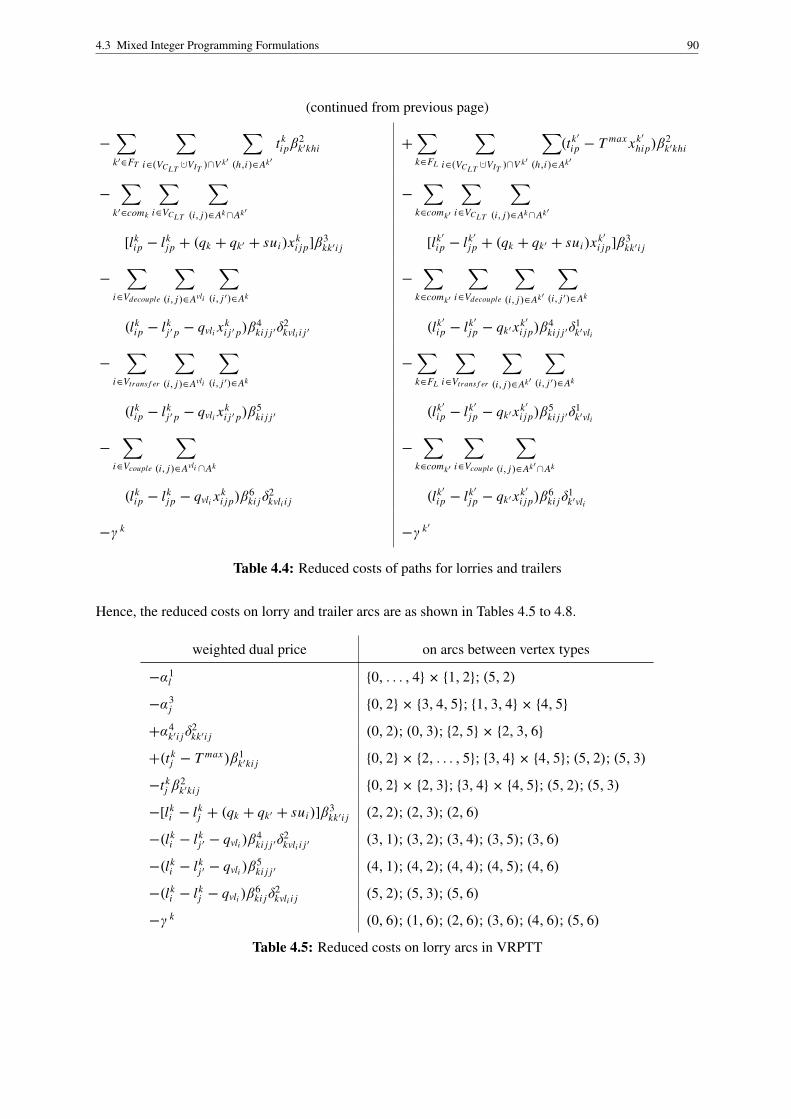
4.3 Mixed Integer Programming Formulations 90
(continued from previous page)
−
∑k′∈FT
∑i∈(VCLT
·∪VIT )∩V k′
∑(h,i)∈Ak′
tkipβ
2k′khi +
∑k∈FL
∑i∈(VCLT
·∪VIT )∩V k′
∑(h,i)∈Ak′
(tk′i p − T max xk′
hip)β2k′khi
−
∑k′∈comk
∑i∈VCLT
∑(i, j)∈Ak∩Ak′
−
∑k∈comk′
∑i∈VCLT
∑(i, j)∈Ak∩Ak′
[lkip − lk
jp + (qk + qk′ + sui )xki j p]β3
kk′i j [lk′i p − lk′
j p + (qk + qk′ + sui )xk′i j p]β3
kk′i j
−
∑i∈Vdecouple
∑(i, j)∈Avli
∑(i, j ′)∈Ak
−
∑k∈comk′
∑i∈Vdecouple
∑(i, j)∈Ak′
∑(i, j ′)∈Ak
(lkip − lk
j ′ p − qvli xki j ′ p)β
4ki j j ′δ
2kvli i j ′ (lk′
i p − lk′j p − qk′xk′
i j p)β4ki j j ′δ
1k′vli
−
∑i∈Vtrans f er
∑(i, j)∈Avli
∑(i, j ′)∈Ak
−
∑k∈FL
∑i∈Vtrans f er
∑(i, j)∈Ak′
∑(i, j ′)∈Ak
(lkip − lk
j ′ p − qvli xki j ′ p)β
5ki j j ′ (lk′
i p − lk′j p − qk′xk′
i j p)β5ki j j ′δ
1k′vli
−
∑i∈Vcouple
∑(i, j)∈Avli ∩Ak
−
∑k∈comk′
∑i∈Vcouple
∑(i, j)∈Ak′∩Ak
(lkip − lk
jp − qvli xki j p)β
6ki jδ
2kvli i j (lk′
i p − lk′j p − qk′xk′
i j p)β6ki jδ
1k′vli
−γ k−γ k′
Table 4.4: Reduced costs of paths for lorries and trailers
Hence, the reduced costs on lorry and trailer arcs are as shown in Tables 4.5 to 4.8.
weighted dual price on arcs between vertex types
−α1l {0, . . . , 4} × {1, 2}; (5, 2)
−α3j {0, 2} × {3, 4, 5}; {1, 3, 4} × {4, 5}
+α4k′i jδ
2kk′i j (0, 2); (0, 3); {2, 5} × {2, 3, 6}
+(tkj − T max)β1
k′ki j {0, 2} × {2, . . . , 5}; {3, 4} × {4, 5}; (5, 2); (5, 3)
−tkj β
2k′ki j {0, 2} × {2, 3}; {3, 4} × {4, 5}; (5, 2); (5, 3)
−[lki − lk
j + (qk + qk′ + sui )]β3kk′i j (2, 2); (2, 3); (2, 6)
−(lki − lk
j ′ − qvli )β4ki j j ′δ
2kvli i j ′ (3, 1); (3, 2); (3, 4); (3, 5); (3, 6)
−(lki − lk
j ′ − qvli )β5ki j j ′ (4, 1); (4, 2); (4, 4); (4, 5); (4, 6)
−(lki − lk
j − qvli )β6ki jδ
2kvli i j (5, 2); (5, 3); (5, 6)
−γ k (0, 6); (1, 6); (2, 6); (3, 6); (4, 6); (5, 6)
Table 4.5: Reduced costs on lorry arcs in VRPTT

4.3 Mixed Integer Programming Formulations 91
weighted dual price on arcs between vertex types
−α2j δ
1k′vlj
(0, 3); (2, 3); {3, 4} × {4, 5}; (5, 3)
+α3j δ
1k′vlj
(0, 3); (2, 3); {3, 4} × {4, 5}; (5, 3)
−α4k′i j {0, 2, 5} × {2, 3}; (2, 6); (5, 6)
−tk′j β1
k′ki j {0, 2} × {2, 3}; {3, 4} × {4, 5}; (5, 2); (5, 3)
+(tk′j − T max)β2
k′ki j {0, 2} × {2, 3}; {3, 4} × {4, 5}; (5, 2); (5, 3)
−[lk′i − lk′
j + (qk + qk′ + sui )]β3kk′i j (2, 2); (2, 3); (2, 6)
−(lk′i − lk′
j − qk′)β4ki j j ′δ
1k′vli (3, 4); (3, 5)
−(lk′i − lk′
j − qk′)β5ki j j ′δ
1k′vli (4, 4); (4, 5)
−(lk′i − lk′
j − qk′)β6ki jδ
1k′vli (5, 2); (5, 3); (5, 6)
−γ k′ (0, 6); (2, 6); (3, 6); (4, 6); (5, 6)
Table 4.6: Reduced costs on trailer arcs in VRPTT
α1 α2 α3 α4 β1 β2 β3 β4 β5 β6 γ(0, 1) X(0, 2) X X X X(0, 3) X X X X(0, 4) X X(0, 5) X X(0, 6) X(1, 1) X(1, 2) X(1, 4) X(1, 5) X(1, 6) X(2, 1) X(2, 2) X X X X X(2, 3) X X X X X(2, 4) X X(2, 5) X X(2, 6) X X X(3, 1) X X(3, 2) X X(3, 4) X X X X(3, 5) X X X X(3, 6) X X(4, 1) X X(4, 2) X X(4, 4) X X X X(4, 5) X X X X(4, 6) X X(5, 2) X X X X X(5, 3) X X X X(5, 6) X X X
Table 4.7: Reduced costs on lorry arcs in VRPTT

4.3 Mixed Integer Programming Formulations 92
α1 α2 α3 α4 β1 β2 β3 β4 β5 β6 γ
(0, 2) X X X(0, 3) X X X X X(0, 6) X(2, 2) X X X X(2, 3) X X X X X X(2, 6) X X X(3, 4) X X X X X(3, 5) X X X X X(4, 4) X X X X X(4, 5) X X X X X(5, 2) X X X X(5, 3) X X X X X X(5, 6) X X X
Table 4.8: Reduced costs on trailer arcs in VRPTT
The objective functions of the pricing problems for lorries and trailers can therefore be written as shownin Table 4.9.
O F sub,k|k∈FL = O F sub,k′
|k′∈FT =∑(i, j)∈Ak
cki j x
ki j + ctime
k (tkd − tk
o )∑
(i, j)∈Ak′
ck′i j x
k′i j
−
∑l∈RW LC
∑i∈V l
C
∑(h,i)∈Ak
α1l xk
hi
−
∑i∈VIT
∑(h,i)∈Ak′
α2i xk′
hi
δ1k′vli
−
∑i∈VIT
∑(h,i)∈Ak
α3i xk
hi +
∑i∈VIT
∑(h′,i)∈Ak′
α3i xk′
hi
δ1k′vli
+
∑k′∈FT
∑(i, j)∈Ak′\Asingle
k′
α4k′i j x
ki j
δ2kk′i j −
∑(i, j)∈Ak′\Asingle
k′
α4k′i j x
k′i j
+
∑k′∈FT
∑i∈(VCLT
·∪VIT )∩V k′
∑(h,i)∈Ak
−
∑k∈FL
∑i∈(VCLT
·∪VIT )∩V k′
∑(h,i)∈Ak
β1k′khi t
k′i
(β1
k′khi tki − β1
k′khi Tmax xk
hi
)−
∑k′∈FT
∑i∈(VCLT
·∪VIT )∩V k′
∑(h,i)∈Ak′
β2k′khi t
ki +
∑k∈FL
∑i∈(VCLT
·∪VIT )∩V k′
∑(h,i)∈Ak′(
β2k′khi t
k′i − β2
k′khi Tmax xk′
hi
)−
∑k′∈comk
∑i∈VCLT
∑(i, j)∈Ak∩Ak′
−
∑k∈comk′
∑i∈VCLT
∑(i, j)∈Ak∩Ak′[
β3kk′i j l
ki − β3
kk′i j lkj + β3
kk′i j (qk + qk′ + sui )xki j
] [β3
kk′i j lk′i − β3
kk′i j lk′j + β3
kk′i j (qk + qk′ + sui )xk′i j
](continued on next page)

4.3 Mixed Integer Programming Formulations 93
(continued from previous page)
−
∑i∈Vdecouple
∑(i, j)∈Avli
∑(i, j ′)∈Ak
−
∑k∈comk′
∑i∈Vdecouple
∑(i, j)∈Ak′
∑(i, j ′)∈Ak
(β4
ki j j ′lki − β4
ki j j ′lkj ′ − β4
ki j j ′qvli xki j ′
)δ2
kvli i j ′
(β4
ki j j ′lk′i − β4
ki j j ′lk′j − β4
ki j j ′qk′xk′i j
)δ1
k′vli
−
∑i∈Vtrans f er
∑(i, j)∈Avli
∑(i, j ′)∈Ak
−
∑k∈FL
∑i∈Vtrans f er
∑(i, j)∈Ak′
∑(i, j ′)∈Ak(
β5ki j j ′l
ki − β5
ki j j ′lkj ′ − β5
ki j j ′qvli xki j ′
) (β5
ki j j ′lk′i − β5
ki j j ′lk′j − β5
ki j j ′qk′xk′i j
)δ1
k′vli
−
∑i∈Vcouple
∑(i, j)∈Avli ∩Ak
−
∑k∈comk′
∑i∈Vcouple
∑(i, j)∈Ak′∩Ak(
β6ki j l
ki − β6
ki j lkj − β6
ki j qvli xki j
)δ2
kvli i j
(β6
ki j lk′i − β6
ki j lk′j − β6
ki j qk′xk′i j
)δ1
k′vli
−γ k−γ k′
Table 4.9: Objective functions of pricing problems in VRPTT
The dual prices for the logically coupling constraints (4.60e)–(4.60j), respectively, the values of thedual variables β in (4.70), induce linear costs on the vertices. These costs depend on the time and loadvariables. Instead of considering them at the vertices, they can be put on the arcs incident to the respectivevertices. Hence, the decisive observation is:
The costs of traversing an arc (i, j) in a pricing problem subnetwork are a function of the service starttime at i and the vehicle load at i and j .
4.3.4.3 Identical Pricing Problems
If all lorries are identical, i.e., if there is only one type of lorry, the problem is symmetric with respectto the lorries, i.e., the subnetworks for the lorries are structurally identical, and only one lorry pricingproblem has to be considered. There are no effects on the trailer pricing problems.
If all trailers are identical, the subnetworks for the trailers are structurally identical as well. However,it is not possible to exploit this fact. Neither the size of a lorry or trailer pricing problem subnetworknor the number of trailer pricing problems to be considered can be reduced. This is because the aboveformulation is based on a network with one vertex per physical transshipment location, time window, andtrailer, and the number of these transshipment vertices specifies the number of times a load transfer at aphysical transshipment location can be performed. Consequently, the number of transshipment verticesin the lorry pricing problem must remain the same whether or not the trailers are identical, and eachtrailer still has its own distinct subnetwork.
In short:
The VRPTT is easier if all lorries are the same, but it is not easier if all trailers are the same.
If all lorries are identical, and whether or not all trailers are identical, let PL be the common set of extremepoints for lorries, let cL
i j and ctimeL be the objective function coefficients for lorries for the distance- and
time-dependent costs, let x Li j be the common binary arc variable for the lorries on arc (i, j), let x L
i jp be thecommon binary arc variable for the lorries on arc (i, j) for path p, let t L
ip be the common time variablefor the lorries at vertex i on path p, and define
λLp :=
∑k∈FL
λkp ∀ p ∈ PL . (4.71)

4.3 Mixed Integer Programming Formulations 94
The IMP can then be formulated as follows:∑p∈PL
∑(i, j)∈AL
cLi j x
Li jp
λLp +
∑k′∈FT
∑p∈Pk′
∑(i, j)∈Ak′
ck′i j x
k′i j p
λk′p +
∑p∈PL
ctimeL (t L
dp − t Lop)λ
Lp → min (4.72)
subject to
∑p∈PL
∑i∈V l
C
∑(h,i)∈AL
x Lhip
λLp = 1 ∀ l ∈ RW LC (4.73a)
∑p∈Pvli
∑(h,i)∈Avli
xvlihip
λvlip 5 1 ∀ i ∈ VIT (4.73b)
∑p∈PL
∑(h,i)∈AL
x Lhip
λLp −
∑p∈Pvli
∑(h′,i)∈Avli
xvlih′i p
λvlip 5 0
∀ i ∈ VIT (4.73c)∑p∈Pk′
xk′i j pλ
k′p −
∑p∈PL
x Li jpλ
Lp 5 0 ∀ k ′ ∈ FT , (i, j) ∈ Ak′
\ Asinglek′ (4.73d)
∑p∈Pk′
tk′i pλ
k′p −
∑p∈PL
t Lipλ
Lp + T max
∑p∈PL
x Lhipλ
Lp 5 T max
∀ k ′ ∈ FT , i ∈ (VCLT·∪ VIT ) ∩ V k′, (h, i) ∈ AL (4.73e)∑
p∈PL
t Lipλ
Lp −
∑p∈Pk′
tk′i pλ
k′p + T max
∑p∈Pk′
xk′hipλ
k′p 5 T max
∀ k ′ ∈ FT , i ∈ (VCLT·∪ VIT ) ∩ V k′, (h, i) ∈ Ak′ (4.73f)∑
p∈PL
(l Lip − l L
jp
)λL
p
+
∑p∈Pk′
(lk′i p − lk′
j p
)λk′
p + (qL + qk′ + sui )
∑p∈PL
x Li jpλ
Lp +
∑p∈Pk′
xk′i j pλ
k′p
5 2qL + 2qk′ + sui
∀ i ∈ VCLT , k ′ ∈ FT , (i, j) ∈ AL∩ Ak′ (4.73g)∑
p∈Pvli
(lvlii p − lvli
j p
)λvli
p +∑p∈PL
(l Lip − l L
j ′ p
)λL
p +∑
p∈Pvli
(qvli x
vlii j p
)λvli
p +∑p∈PL
(qvli x
Li j ′ p
)λL
p 5 2qvli
∀ i ∈ Vdecouple, (i, j) ∈ Avli , (i, j ′) ∈ AL (4.73h)∑p∈Pvli
(lvlii p − lvli
j p
)λvli
p +∑p∈PL
(l Lip − l L
j ′ p
)λL
p +∑
p∈Pvli
(qvli x
vlii j p
)λvli
p +∑p∈PL
(qvli x
Li j ′ p
)λL
p 5 2qvli
∀ i ∈ Vtrans f er , (i, j) ∈ Avli , (i, j ′) ∈ AL (4.73i)

4.3 Mixed Integer Programming Formulations 95
∑p∈Pvli
(lvlii p − lvli
j p
)λvli
p +∑p∈PL
(l Lip − l L
jp
)λL
p +∑
p∈Pvli
(qvli x
vlii j p
)λvli
p +∑p∈PL
(qvli x
Li jp
)λL
p 5 2qvli
∀ i ∈ Vcouple, (i, j) ∈ Avli ∩ AL (4.73j)
λLp =
∑k∈FL
λkp ∀ p ∈ PL (4.73k)
λLp = 0 ∀ p ∈ PL (4.73l)∑
p∈PL
λkp 5 1 ∀ k ∈ FL (4.73m)
∑p∈Pk′
λk′p 5 1 ∀ k ′ ∈ FT (4.73n)
λkp = 0 ∀ k ∈ F, p ∈ Pk (4.73o)
x Li j =
∑p∈PL
x Li jpλ
Lp ∀ (i, j) ∈ AL (4.73p)
x Li j ∈ {0, 1} ∀ (i, j) ∈ AL (4.73q)
xk′i j =
∑p∈Pk′
xk′i j pλ
k′p ∀ k ′ ∈ FT , (i, j) ∈ Ak′ (4.73r)
xk′i j ∈ {0, 1} ∀ k ′ ∈ FT , (i, j) ∈ Ak′ (4.73s)
The dual variables in (4.70), the reduced costs for paths and arcs, and the objective functions for thepricing problems given in Tables 4.4–4.9 then lose their k indices (for the lorries), as (4.73k) and (4.73m)imply ∑
p∈PL
λLp =
∑p∈PL
∑k∈FL
λkp =
∑k∈FL
∑p∈PL
λkp 5
∑k∈FL
1 = |FL |, (4.74)
cf. Desaulniers et al. 1998, p. 85; i.e., (4.73k) and (4.73m) can be replaced by (4.74). Indeed, the righthand side in constraint (4.74) can be set to an arbitrarily high value, respectively, can be dropped alto-gether, reflecting a situation where the number of lorries is unlimited.
Note that all x Li j variables remain binary, because the arc (o, d) was removed. This means that, in any
feasible solution, no arc is traversed by more than one lorry, and this is why the third summand in theabove objective function correctly accounts for the time-dependent costs.
The LP relaxation of (4.72)–(4.73), however, is weaker than that of (4.68)–(4.69), because the disaggre-gated constraints (4.69e)–(4.69j) are stronger than the aggregated constraints (4.73e)–(4.73j).
In practice, there are often two types of lorry and two types of trailer, and only one lorry type canpull both trailer types. Generally speaking, if there are several subsets or classes of identical lorries,the aggregation performed in (4.72)–(4.73) can be performed for each class separately. The L indicesmust then be sub-indexed, and slight modifications of (4.72)–(4.73) and a little more writing effort arenecessary (therefore, this is not fully carried out here): Let KL be the number of lorry classes, and let{L1, . . . , L KL } be the set of lorry classes. Then, modified vehicle compatibility functions comLr for the

4.3 Mixed Integer Programming Formulations 96
lorry classes and ˜comk′ for the trailers are necessary. The second term on the left hand side of (4.73d),for example, becomes
−
∑Lr∈
˜comk′∩{Lr∈{L1,...,L KL }:(i, j)∈ALr }
∑p∈PLr
x Lri j pλ
Lrp .
It is also possible to aggregate over identical vehicles in the arc variable formulation (4.59)–(4.62).However, the underlying network must then be modified to make sure that the resource variables for loadand time can be updated correctly at the end of each vehicle’s itinerary. This is not a problem at customeror transshipment vertices, because only one lorry and one trailer (at most) visit such vertices, but the enddepot vertex is reached by all vehicles. Hence, an end depot vertex for each trailer and for each lorrymust be introduced (which means that the number of vehicles cannot be arbitrary). These new depotvertices replace the single depot vertex, and they can be reached from all vertices that have emanatingarcs leading to the end depot vertex in the original network. Moreover, an arc from each trailer depotvertex dk′ for trailer k ′ to each lorry depot vertex dk for lorry k with k ∈ comk′ must be added. Noarcs emanate from the lorry depot vertices. The resulting modifications to formulation (4.59)–(4.62) arestraightforward.
4.3.5 Modified Formulations
The turn variable formulation requires that each arc is traversed at most once, the arc variable and thepath variable formulations require that each vertex is visited at most once. Without such postulates,unless good upper bounds for the number of traversals of each arc by each vehicle, respectively, for themaximum number of visits of each vehicle at each vertex, can be determined, it is impossible to statea mathematical programming formulation: If it is not clear how many times an arc may be traversedor a vertex may be visited, there is no way to index the load and time variables. This section presentspossible modifications to the arc variable formulation that overcome this difficulty, albeit at the cost ofan enlarged network and at the cost of loss of precision. The decisive ideas are
• to discretize the load transfer amounts, i.e., to specify all possible load transfer amounts at eachtransshipment location, and
• to introduce a fixed schedule network for the trailers (or even for lorries and trailers) to get rid ofthe ‘same departure time constraints’ (4.60e) and (4.60f).
The discretization approach is a technique that is also used in the context of the split delivery vehiclerouting problem, where the fraction of a certain customer’s demand satisfied by a certain vehicle is re-stricted to a discrete number of possible values, cf. Dror/Langevin 2000, p. 315. Acyclic fixed-scheduletime-space networks are used in many papers on time-constrained vehicle routing and scheduling prob-lems (see the survey by Desaulniers et al. 1998).
If only the load transfer amounts are discretized, (4.59)–(4.62) changes as follows:
• S plta , the set of possible load transfer amounts, is specified. To keep the network size limited,|S plta
| 5 4. For each triple (k ′, l, τ ), i.e., for each transshipment vertex in (4.59)–(4.62), there are|S plta
| transshipment vertices vk′lτ s , s ∈ S plta , each of which represents a load transfer of s units of
load to trailer k ′ at location l in time window τ . The load of a lorry visiting such a transshipmentvertex then decreases by s; the load of the pertinent trailer increases by s. The arc traversal timesof arcs leaving transshipment vertices are changed to reflect the now known service times at theirtails, similar to the arcs leaving customer vertices.
If the definition of the supply function, su, is changed such as to reflect the discretized load transferamounts, the following constraints are affected:
– (4.60h) become

4.3 Mixed Integer Programming Formulations 97
xki j = 1⇒ lk
i − sui 5 lkj ∀ i ∈ Vdecouple, k ∈ comvli , (i, j) ∈ Ak (4.75a)
xvlii j = 1⇒ lvli
i + sui 5 lvlij ∀ i ∈ Vdecouple, (i, j) ∈ Avli , (4.75b)
and (4.60i) and (4.60j) change accordingly.
– (4.61c) become redundant.
– (4.61g) and (4.61h) become redundant, because of the modified constraints (4.60h), (4.60i),and (4.60j).
– (4.61k) and (4.61l) become redundant, as they can be subsumed under constraints (4.61j) byalso considering i ∈ VIT there, respectively, by considering (4.61j) also for i ∈ VIT , (i, j) ∈Avli .
• For the load update constraints at trailer customers, several options exist:
– Assume the complete supply of the customer is loaded onto the lorry.
– Assume the complete supply of the customer is loaded onto the trailer.This and the previous option are restrictive in the sense that a lorry-trailer combination maynot be able to visit a trailer customer, although the overall remaining capacity of the combina-tion is still sufficient to collect the customer’s supply, because the remaining capacity of thelorry or trailer is too small. These options may even lead to infeasibilities if there are trailercustomers with a supply greater than the capacity of the biggest available lorry or trailer.
– Assume several allowed partitions of the supply to divide it up between lorry and trailer.
Equivalently, the original VRPTT network can be enlarged by adding |S plta| − 1 parallel arcs for each
arc emanating from a transshipment vertex (and possibly from a trailer customer vertex).
The problem when only these changes are made is that the same departure time constraints (4.60e) and(4.60f) remain. To avoid them, the network can be further changed as follows. For each customer andtransshipment vertex resulting from the above modifications, the associated time window is interpreteddifferently: For a vertex i with a time window of [twai , twbi ], twbi is viewed as the point in time whereany vehicle visiting i leaves i . Waiting is still allowed. This makes the time variables redundant. Theservice times for all services to be performed at any vertex are simply added to the traversal times of theentering or emanating arcs. The planning horizon is then partitioned into subperiods, and, consideringthe original time windows of the locations, one vertex for each customer and transshipment vertex of theoriginal network is introduced. This leads to an acyclic network.
This constitutes a very restrictive approach, too. The inaccuracy thus introduced depends largely on thenumber of subperiods. The more subperiods there are, the more accurate the resulting network is. How-ever, there is a trade-off in that more subperiods lead to an increased network size. The subperiod lengthdesirable for realistic instances, together with the length of the planning horizon, may result in a networkof prohibitively large size.
A possible compromise consists in making fixed schedule vertices only for the transshipment locationsand the trailer customers and keeping the time variables for the lorries. The update of the time variablesat the fixed schedule vertices then works as follows. If the departure time at a fixed schedule vertexi is t at the outset, the time window of i is set to [twai , t − t service
i ], where t servicei corresponds to the
time needed to collect the customer supply, respectively, the time needed to transfer the fixed amount ofload. The traversal time of all arcs emanating from i is then increased by t service
i . Consider the examplesituation depicted in Figure 4.7. Vertices i1, i2, i3 and the unnamed vertices correspond to one physicaltransshipment location l and one trailer k ′ during different subperiods/time windows ([8:01, 8:20], [8:21,8:40], and [8:41, 9:00]) and for different load transfer amounts (0, 5 and 10 units). In the figure, lorryk1 pulls trailer k ′ to transshipment vertex i1, which has a twenty-minute time window of [8:01, 8:20] and

4.3 Mixed Integer Programming Formulations 98
corresponds to a load transfer amount of zero. k1 decouples k ′ and moves on along arc a1. k ′ performsa temporal and logical move to vertex i2, which corresponds to l during the time window [8:21, 8:40]and to a load transfer amount of five units. This load is transferred by lorry k2, which arrives at i2 via arca2 and leaves location l along arc a3. By definition, k ′ is at vertex i2 at 8:21, and the load transfer maystart as soon as k2 arrives, as long as it arrives soon enough to complete the transfer of five units of loadby 8:40. Hence, if a load transfer of five units takes five minutes, the time window for i2 is set to [8:21,8:35]. Trailer k ′ performs yet another temporal and logical move to vertex i3 and is coupled there at 8:41by lorry k3, which arrives along arc a4 and moves on along arc a5, pulling k ′ with it. The only additionalchange to (4.59)–(4.62) is that the beginning of the service of lorry k at trailer customer or transshipmentvertex i is exactly equal to the modified right time window bound twbi .
pppppppppppppppppppppppppppppppppppppppppppppppppppppppppppppppppppppppppppppppppppppppppppppppppppppppppppppppppppppppppppppp
ppppppppppppppppppppppppppppppppppppppppppppppppppp ppppppppppppppppppppppppppppppppppppppppppppppppppppppppppppppppppppppppppppppppppppppppppppppppppppppppppppppppppppppppppppppppppp pppppppppppp ppppppppppppppppppppppppppppppppppppppppppppppppppppppppppppppppppppppppppppppppppppppppppppppppppppppppppppppppppppppppppppppppppp pppppppppppp ppppppppppppppppppppppppppppppppppppppppppppppppppppppppppppppppp
pppppppppppppppppppppppppppppppppppppppppppppppppppppppppppppppppppppppppppppppppppppppp ppppppppppppppppppppppppppppppppppppppppppppppppppp
......................................................................................................................................................................................
...................................................................................................................................................
....................................................................................................
.............
.............
.............
.............
.............
.............................
. . . . . . . . . . ....
..
..
..
..
..
..
...................................................
.......................................
.....
........
........
........
........
........
........
........
........
........
........
........
........
........
........
........
........
........
........
........
........
........
........
........
........
........
........
..........................
....................
�
�
�
�
�
�
�
�
�
Load transfer amounts
0
5
10
Lorry k1
Lorry k2
Lorry k3
Trailer k′
[8:01, 8:20] [8:21, 8:40] [8:41, 9:00]
i1
i2
i3
a1
a2
a3
a4
a5
Figure 4.7: Transshipment vertices with discretized load transfer amounts and fixed schedule
The following cases are possible:
• A trailer is only parked. No load transfer is performed. The trailer is coupled again by the lorrythat parked it or by a different one. This is represented by the trailer moving in time between twoor more vertices corresponding to a load transfer amount of zero.
• The trailer is parked, but not decoupled; only a load transfer is performed. This is represented bythe trailer moving directly with a lorry to a vertex corresponding to a positive load transfer amount,and leaving this vertex again along the same arc as the lorry.
• The lorry pulling the trailer to the transshipment location performs a load transfer, decouples, anda different lorry re-couples the trailer later. This is represented by the trailer moving directly witha lorry to a vertex corresponding to a positive load transfer amount, and then moving logically intime to a vertex corresponding to a load transfer amount of zero.
• Several lorries perform a load transfer to one trailer at one transshipment location. This is schemat-ically depicted in Figure 4.8. The depicted lorry arcs could all represent one and the same lorry, orthey could represent up to four different lorries.
As mentioned at the beginning of this section, the above approach can, strictly speaking, no longer becalled exact. From a practical point of view, it may be argued that it is preferable to have a heuristicsolution to an exact formulation, i.e., to a formulation that represents reality as correctly and precisely aspossible, than to have an optimal solution to a less exact formulation. However, the idea of discretizingthe load transfer amounts maintains exactness of the formulation in cases where the goods to be collectedat customers are not homogeneous.

4.4 A Branch-and-Price Algorithm for the VRPTT? 99
pppppppppppppppppppppppppppppppppppppppppppppppppppppppppppppppppppppppppppppppppppppppppppppppppppppppppppppppppppppppppppppppp
ppppppppppppppppppppppppppppppppppppppppppppp ppppppppppppppppppppppppppppppppppppppppppppppppppppppppppppppppppppppppppppppppppppppppppppppppppppppp pppppppppppp ppppppppppppppppppppppppppppppppppppppppppppppppppppppppppppppppppppppppppppppppppppppppppppppppppppppp pppppppppppp ppppppppppppppppppppppppppppppppppppppppppppppppppppppppppppppppppppppppppppppppppppppppppppppppppppppppppppppppppppppppppppppppppp pppppppppppp pppppppppppppppppppppppppppppppppppppppppppppppppppppppppppppppppppppppppppppppppppppppppppppppppppppppppppppppppppppppppppppppppppppppppppppppppppppppp
ppppppppppppppppppppppppppppppppppppppppppppppppppp
.............................................................................................................................................................................
......................................................................................................................................................
....................
....................
....................
....................
....................
....................
....................
....................
..............
............
..........................................................................................................................................................
....................
....................
....................
....................
....................
....................
....................
....................
..............
............
....................
....................
....................
....................
....................
....................
.....................................
.....................................................................................................................................................
..............................................................................................................................................................
...................................................
........
........
........
........
........
........
........
........
........
........
........
........
........
........
........
........
........
........
........
........
........
........
........
........
........
........
..........................
....................
...........................................................................................................................................................................................................................................................
...
�
�
�
�
�
�
�
�
�
�
�
�
Load transfer amounts
0
5
10
Lorries
Trailer
Time
Figure 4.8: Several lorries perform a load transfer to one trailer at one transshipment location
4.4 A Branch-and-Price Algorithm for the VRPTT?
The path variable formulation given above can, in principle, be used to solve the VRPTT by branch-and-price. However, the interdependencies between lorries and trailers cause considerable difficulties for thesolution of the pricing problems. These difficulties are discussed in this section.
As mentioned above, the pricing problems for the VRPTT are ESPPRCs, and for each vehicle, an ESP-PRC must be solved. If these ESPPRCs are to be solved by a labelling algorithm, the resources forvehicle k are:
• an unconstrained, cardinally scaled resource for costs and
• one cardinally scaled resource for each of the two resource variables used in (4.59)–(4.62), i.e., forload and time
The unconstrained resource measuring the costs is denoted by r cost . The corresponding resource variableis σ cost
i , and the REF is f rcost. The resource for time is r time with resource variable σ time
i and REF f r time,
and the resource for load is r load with resource variable σ loadi and REF f r load
. The resource windows ata vertex i are ]−∞,+∞[ for cost, [twai , twbi ] for time, and [0, qk] for load. The REFs for the VRPTTpricing problem for lorry k ∈ F for all arcs (i, j) ∈ Ak are as follows:
f rcost
i j (σ costi , σ time
o , σ timej , σ load
i , σ loadj ) = σ cost
i + cki j (σ
timej , σ load
i , σ loadj )+ (σ time
j − σ timeo )ctime
k (4.76)
f r time
i j (σ timei , σ load
i , σ loadj ) =
max{
twaj , σtimei + τ tr
i j
}, i ∈ {o} ·∪ VC
max{
twaj , σtimei + τ tr
i j + (σ loadi − σ load
j )τ lt}, i ∈ VIT
(4.77)
f r load(σ load
i ) =
σ load
i , i ∈ {o} ·∪ VCLT
σ loadi + sui , i ∈ VCL
0 , i ∈ VIT
(4.78)
The REFs for the VRPTT pricing problem for trailer k ′ ∈ FT on arc (i, j) ∈ Ak′ are as follows:
f rcost
i j (σ costi , σ time
i , σ timej , σ load
i , σ loadj ) = σ cost
i + cki j (σ
timej , σ load
i , σ loadj ) (4.79)
f r time
i j (σ timei , σ load
i , σ loadj ) =
max{
twaj , σtimei + τ tr
i j
}, i ∈ {o} ·∪ VCLT
max{
twaj , σtimei + τ tr
i j + (σ loadj − σ load
i )τ lt}, i ∈ VIT
(4.80)

4.4 A Branch-and-Price Algorithm for the VRPTT? 100
f r load(σ load
i ) = σ loadi (4.81)
cki j (σ
timej , σ load
i , σ loadj ) is the function specifying the reduced costs on arc (i, j) according to Tables 4.5
and 4.6.
The first difficulty that arises when trying to solve the lorry pricing problems by a labelling algorithm isthe time-dependent costs (the last term in the cost REF for lorries). With time-dependent costs and thepossibility of having to wait at a vertex (due to the static and dynamic time windows), it need no longerbe optimal to leave the start depot vertex at time zero, i.e., to set σ time
o = 0. Desaulniers/Villeneuve2000 have shown that such a problem can be solved as an (E)SPPRC by introducing two additional re-sources that take into account the time costs. The definition and interpretation of these resources is ratherinvolved. The reader interested in the details is referred to the above paper. Suffice it here to say thatthe implementation (in a computer code) is straightforward, so if it were only for the time-dependentcosts, the lorry pricing problem in the VRPTT could be solved by a labelling algorithm without muchprogramming or computational overhead.
However, there are more serious issues to consider: To solve (E)SPPRCs by a labelling algorithm, it ishighly desirable that all REFs possess the following two properties (Desaulniers et al. 1998, p. 82):
(i) All REFs for an arc (i, j) should depend only on the resource vector at i .If this property holds, intermediate resource levels can be computed which provide (good) lowerbounds for the values of the resource variables.
(ii) All REFs should be non-decreasing.If this property holds, the lowest costs at vertex j are always attained at the lowest feasible valuesof the resource variables.
Unfortunately, neither property is fulfilled in the VRPTT pricing problems. To see why this is the caseand why this is a difficulty, first consider the REFs for cost, time, and load in the VRPTW:
f rcost
i j (σ costi ) = σ cost
i + ci j
f r time
i j (σ timei ) = max{twaj , σ
timei + τ tr
i j }
f r load
i j (σ loadi ) = σ load
i + sui
It is easy to see that these REFs fulfil the above two properties. For example, the load after having visitedcustomer i is at least as much as the load at the point in time when customer i was reached plus customeri’s supply, i.e., σ load
i + sui is a valid lower bound. But it is more than that: It is a sharp bound. The loadafter having visited customer i can safely be assumed to be equal to σ load
i + sui . When extending a labelat i along the arc (i, j), it is not necessary to create a label with a different value for σ load
j . The sameholds for the other two resources.
In the VRPTT, things are different. To see that the first property is violated, observe that constraints(4.60e)–(4.60j), which determine the update of the time and load variables at trailer customer and trans-shipment vertices, are logically coupling constraints. This means that the REFs for time and load of avehicle at such vertices depend on the load of other vehicles. Such REFs are not possible. However,as indicated in (4.76)–(4.81), valid lower bounds can still be computed. So, property (i) is not ‘really’violated in a narrow sense, but the bounds cannot directly be used for the resource updates in a labellingalgorithm. Consider, for example, the lorry REFs. All three of them are interdependent. The value of theREF for time at intermediate vertices, i.e., the value of the resource variable for time at vertex j , σ time
j ,depends not only on σ time
i , but also on the values of the resource variables for load at the tail and headof an arc (i, j). The value of the REF for cost, in turn, depends on the values of the resource variablesfor time. A sequential computation of the REFs is possible in a labelling algorithm, so the REF for load
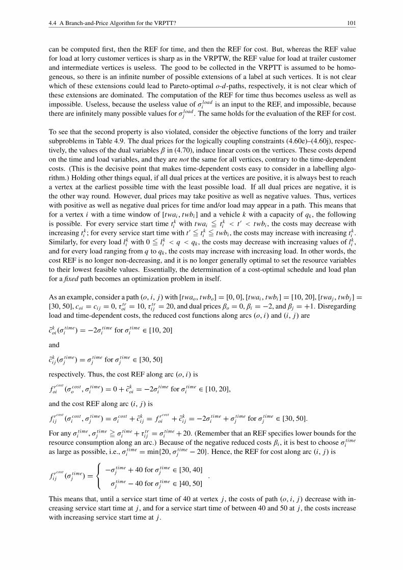
4.4 A Branch-and-Price Algorithm for the VRPTT? 101
can be computed first, then the REF for time, and then the REF for cost. But, whereas the REF valuefor load at lorry customer vertices is sharp as in the VRPTW, the REF value for load at trailer customerand intermediate vertices is useless. The good to be collected in the VRPTT is assumed to be homo-geneous, so there is an infinite number of possible extensions of a label at such vertices. It is not clearwhich of these extensions could lead to Pareto-optimal o-d-paths, respectively, it is not clear which ofthese extensions are dominated. The computation of the REF for time thus becomes useless as well asimpossible. Useless, because the useless value of σ load
i is an input to the REF, and impossible, becausethere are infinitely many possible values for σ load
j . The same holds for the evaluation of the REF for cost.
To see that the second property is also violated, consider the objective functions of the lorry and trailersubproblems in Table 4.9. The dual prices for the logically coupling constraints (4.60e)–(4.60j), respec-tively, the values of the dual variables β in (4.70), induce linear costs on the vertices. These costs dependon the time and load variables, and they are not the same for all vertices, contrary to the time-dependentcosts. (This is the decisive point that makes time-dependent costs easy to consider in a labelling algo-rithm.) Holding other things equal, if all dual prices at the vertices are positive, it is always best to reacha vertex at the earliest possible time with the least possible load. If all dual prices are negative, it isthe other way round. However, dual prices may take positive as well as negative values. Thus, verticeswith positive as well as negative dual prices for time and/or load may appear in a path. This means thatfor a vertex i with a time window of [twai , twbi ] and a vehicle k with a capacity of qk , the followingis possible. For every service start time tk
i with twai 5 tki < t ′ < twbi , the costs may decrease with
increasing tki ; for every service start time with t ′ 5 tk
i 5 twbi , the costs may increase with increasing tki .
Similarly, for every load lki with 0 5 lk
i < q < qk , the costs may decrease with increasing values of lki ,
and for every load ranging from q to qk , the costs may increase with increasing load. In other words, thecost REF is no longer non-decreasing, and it is no longer generally optimal to set the resource variablesto their lowest feasible values. Essentially, the determination of a cost-optimal schedule and load planfor a fixed path becomes an optimization problem in itself.
As an example, consider a path (o, i, j) with [twao, twbo] = [0, 0], [twai , twbi ] = [10, 20], [twaj , twbj ] =[30, 50], coi = ci j = 0, τ tr
oi = 10, τ tri j = 20, and dual prices βo = 0, βi = −2, and βj = +1. Disregarding
load and time-dependent costs, the reduced cost functions along arcs (o, i) and (i, j) are
ckoi (σ
timei ) = −2σ time
i for σ timei ∈ [10, 20]
and
cki j (σ
timej ) = σ time
j for σ timej ∈ [30, 50]
respectively. Thus, the cost REF along arc (o, i) is
f rcost
oi (σ costo , σ time
i ) = 0+ ckoi = −2σ time
i for σ timei ∈ [10, 20],
and the cost REF along arc (i, j) is
f rcost
i j (σ costi , σ time
j ) = σ costi + ck
i j = f rcost
oi + cki j = −2σ time
i + σ timej for σ time
j ∈ [30, 50].
For any σ timei , σ time
j = σ timei + τ tr
i j = σ timei + 20. (Remember that an REF specifies lower bounds for the
resource consumption along an arc.) Because of the negative reduced costs βi , it is best to choose σ timei
as large as possible, i.e., σ timei = min{20, σ time
j − 20}. Hence, the REF for cost along arc (i, j) is
f rcost
i j (σ timej ) =
−σ timej + 40 for σ time
j ∈ [30, 40]
σ timej − 40 for σ time
j ∈ ]40, 50].
This means that, until a service start time of 40 at vertex j , the costs of path (o, i, j) decrease with in-creasing service start time at j , and for a service start time of between 40 and 50 at j , the costs increasewith increasing service start time at j .

4.4 A Branch-and-Price Algorithm for the VRPTT? 102
A non-decreasing REF (of costs against costs) along an arc (i, j) is depicted in Figure 4.9(a). It saysthat, holding other things equal, i.e., for fixed time and load, traversing arc (i, j) reduces the costs by20. Observe that the cumulated resource consumption after extension is less than before the extension.This is not the point with non-decreasing REFs. The point is that the cumulated resource consumptionafter extension is higher, the higher the cumulated resource consumption before extension is. In Figure4.9(b), a not non-decreasing REF (of costs against time) is depicted (it also contains increasing parts, soit cannot be called decreasing). It says that, holding other things equal, i.e., for fixed costs and load, thetotal costs after extension decrease for any service start time up to t ′, and increase for any service starttime later than t ′′.
20
−20
........................... ............
σ costi
........
...................
............f rcosti j
..............................................................
..............................................................
..............................................................
..............................................................
.......................................................
twai t ′ t ′′ twbi
........................... ............
σ timei
........
...................
............f rcosti j
........
.....
........
.....
........
.....
........
.....
........
.....
........
.....
........
.....
........
.....
........
.....
.......
........
.....
........
.....
........
.....
........
.....
........
.....
........
.....
........
.....
........
.....
........
.....
........
..
......................................................................................................................................................................................................................................................................................
...........................................................................................................................................................
(a) (b)
Figure 4.9: (a) Non-decreasing and (b) not non-decreasing REF
The issue is discussed thoroughly in Ioachim et al. 1998 for the case of linear time costs at the vertices.The authors show that the cost function is piecewise linear with a finite number of pieces depending lin-early on the number of vertices in the path, and that the general shape of the cost function is as depictedin Figure 4.9(b) (possibly with t ′ = t ′′). In the VRPTT, the situation is even more complicated, becausethere are linear time and load costs. The cost REF for an arc (i, j) depends on the service start time at iand on the load variables at i and j ; hence, there are four dimensions to consider (the function graph isfour-dimensional).
Summing up, violation of REF properties (i) and (ii) means that it is neither clear how to extend a labelalong an arc, nor when a label at a vertex may be discarded because it is dominated by one or more otherlabels. It is necessary to consider all feasible extensions, but there are uncountably many. The standardresource concept as described in Chapter 2 is not applicable.
In view of these arguments, how can the pricing problem be solved? The following alternatives exist:
• Modify/simplify the problem to avoid not non-decreasing REFs.The issue with the load costs in the VRPTT also arises in the split delivery vehicle routing problem.Dror/Langevin 2000, p. 305 ff., present a column generation approach for this problem, where theydiscretize the number of allowed split deliveries and create one label for each allowed quantity. Ashas been described in Section 4.3.5, the same is possible in the VRPTT, but the resulting algorithmis no longer really exact.
• Extend the approach of Gendreau et al. 2005.Gendreau et al. 2005 use a sophisticated pairwise dominance algorithm based on duality theoryfor solving the split delivery vehicle routing problem without imposing any restrictions on the splitdelivery options. It is as yet unclear whether it is possible to adapt this approach to the VRPTT.

4.4 A Branch-and-Price Algorithm for the VRPTT? 103
• Extend the approach of Ioachim et al. 1998.As mentioned above, Ioachim et al. 1998 consider the SPPRC with linear vertex (time) costs. Theauthors solve the problem with a labelling algorithm by representing the set of feasible resourcevectors by its lower envelope (using adequate resources for storing the description of the lowerenvelope), and by proving that all labels/paths that do not contribute to the lower envelope at avertex are dominated and can be discarded. (This is an example of non-pairwise dominance.)What these authors do, in effect, is to extend the resource concept described in Chapter 2: Theyconsider REFs that are not real-valued, but whose values are intervals (possible values for time andload) or even functions (costs as a function of time and load) instead of scalars. The dominanceprocedure then consists in comparing sets of functions.This seems to be a promising approach. However, Ioachim et al. 1998 describe the lower envelopeof the set of feasible resource vectors by a piecewise linear cost function with at most p+ 1 piecesfor a path of length p. The corresponding four-dimensional envelope for the VRPTT must have(p + 1)3 ‘pieces’, and in general, if there are r resources, there are (p + 1)r ‘pieces’; i.e., thecomplexity of the lower envelope increases exponentially with the number of resources.
• Use results and algorithms from computational geometry and polyhedral theory.For the VRPTT, the set of feasible resource vectors at the end of a (partial) path is a convex poly-tope. If the polytope corresponding to a label can be successfully described by its extreme points,and if the description of the polytope resulting from extending its corresponding label along anarc can be computed, it is possible to use a point-in-polyhedron algorithm (see, e.g., O’Rourke1998, p. 245 ff.) for (not necessarily pairwise) dominance: If the polytope of a path p is com-pletely contained in the polytope of another path, or if the polytope is contained in the union ofthe polytopes of at least two other paths, path p is dominated and can be discarded. Indeed, bothtasks (polytope description by extreme points and computing polytopes/labels resulting from pathextension steps) can be done in a manner similar to the one used by Ioachim et al. 1998 (see pre-vious item). These authors describe their piecewise linear cost functions of (partial) paths by thefunctions’ breakpoints and provide a procedure for computing the breakpoints of a function aftera path extension step. In theory, a point-in-polyhedron test is rather easy for convex polyhedra(needed for pairwise dominance), but somewhat more involved for non-convex polyhedra (neededfor non-pairwise dominance); cf. again O’Rourke 1998, ib.A similar approach may be possible when the polytopes corresponding to labels are described bytheir facets.However, due to numerical problems on today’s digital computers with limited-precision floating-point arithmetic, even an implementation of the approach of Ioachim et al. 1998 in two dimen-sions is non-trivial, and ‘reliable CAD in three dimensions is still ahead of us’ (K. Mehlhorn,2006). Thus, a robust implementation of a point-in-polyhedron algorithm for non-convex four-dimensional polyhedra constitutes a challenge in itself. This is all the more so as such an algorithmis called thousands of times in each iteration of the column generation process at each vertex ofthe branch-and-price tree, so it would also have to run very fast to be useful.
• Solve the ESPPRC by branch-and-cut.The author is aware of only one publication that takes this approach (cf. Bramel/Simchi-Levi2002, p. 91 f.; the authors describe an unpublished technical report where the pricing problemfor the VRP is solved by branch-and-cut). One potential reason for this fact is that, in columngeneration, it is mostly useful to add more than one negative reduced cost column at each iteration.A labelling algorithm always returns all Pareto-optimal solutions (and hence, often more than onenegative reduced cost column), whereas a branch-and-cut algorithm only returns one column (theone with most negative reduced cost).
It was impossible to implement the branch-and-price algorithm for the VRPTT in the time available forthis paper. However, it is doubtful whether an implementation of a branch-and-price algorithm would beable to solve instances of more realistic size than the branch-and-cut algorithm, even if a reasonably fast

4.5 A Branch-and-Cut Algorithm for the Core Problem 104
and robust procedure for the solution of the pricing problems were available. This is because the useful-ness of the dual prices may be limited: The dual prices for the logically coupling constraints are addedto the original costs of the subnetworks’ arcs. In the VRPTW, the only logically coupling constraints arethe ones for customer covering. In the VRPTT, there are several types of logically coupling constraintwhose dual prices may give conflictive indications. If the dual prices for, e.g., the temporal synchro-nization constraints, are negative, and the dual prices for, e.g., the load synchronization constraints, arepositive, the former may be offset by the latter and virtually no dual information may be present in thesubproblems to produce ‘useful’ paths, thus leading to an aggravation of the tailing-off effect often en-countered in column generation.
After these elaborations, it should be evident that the question mark in this section’s headline is not atyping error.
4.5 A Branch-and-Cut Algorithm for the Core Problem
In this section, a branch-and-cut algorithm for the core problem, i.e., the arc variable formulation (4.59)–(4.62), is proposed. The valid inequalities used in the algorithm and the employed branching and enu-meration strategies are described.
4.5.1 Valid Inequalities
The following inequalities are valid for (4.59)–(4.62).
Supply Collection Cut: ∑k∈F
lkd =
∑l∈RW LC
csl (4.82)
This inequality requires that the total customer supply be brought to the depot. In a fractional solution,this might not automatically be the case because of the flow variables that appear in the load updateconstraints (4.60g)–(4.60j) and (4.61d)–(4.61h). To see that the cut constitutes a valid inequality, notethat the following is true in any feasible solution to (4.60)–(4.62): For each lorry (or lorry-trailer com-bination), the complete load after visiting a vertex i and traversing an arc (i, j) (and an arc (i, j ′)) isgreater than or equal to the complete load of the lorry (or lorry-trailer pair) when reaching vertex i plusthe supply of vertex i (because of the load update constraints). Each vehicle reaches the end depot vertexexactly once (because of constraints (4.61a)) and does not leave it again (because there is no arc emanat-ing from the end depot). The ‘=’ sign can also be replaced by ‘=’, because in reality, it is not possibleto collect more supply than there is. Strictly speaking, the inequality is then no longer valid, becausefeasible solutions are cut off. However, none of these solutions can be optimal if the load transfer timesand the time costs are strictly positive.
Trailer Flow Cut: ∑k′∈FT
∑{(i,d)∈Ak′ :i 6=o}
xk′id = num trailers (4.83)
This inequality requires that the flow of trailers into the end depot over arcs other than (o, d) be at leastequal to the minimum number of necessary trailers, num trailers . As the total customer supply must bebrought to the depot (see the supply collection cut), the inequality is valid. A lower bound for num trailers
can be computed as follows. First, sutrailer , the total customer supply that must be brought to the enddepot by a trailer, is computed:
sutrailer=
∑l∈RW LC
csl −∑k∈FL
qk . (4.84)
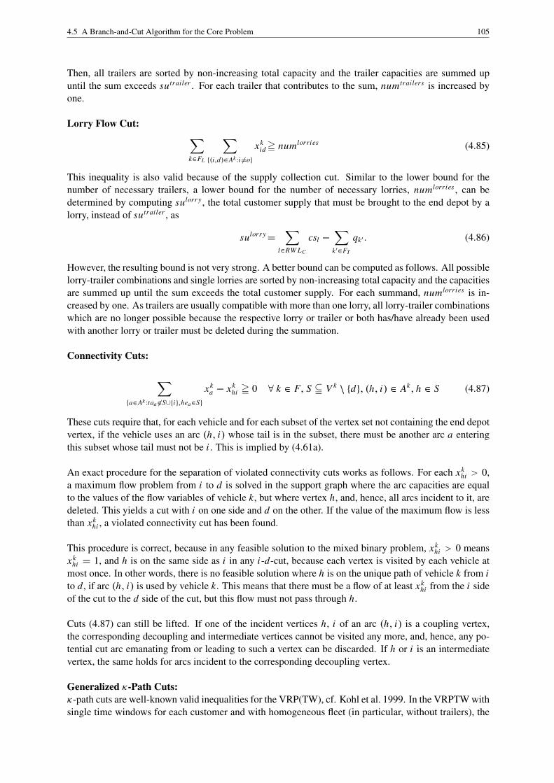
4.5 A Branch-and-Cut Algorithm for the Core Problem 105
Then, all trailers are sorted by non-increasing total capacity and the trailer capacities are summed upuntil the sum exceeds sutrailer . For each trailer that contributes to the sum, num trailers is increased byone.
Lorry Flow Cut: ∑k∈FL
∑{(i,d)∈Ak :i 6=o}
xkid = numlorries (4.85)
This inequality is also valid because of the supply collection cut. Similar to the lower bound for thenumber of necessary trailers, a lower bound for the number of necessary lorries, numlorries , can bedetermined by computing sulorr y , the total customer supply that must be brought to the end depot by alorry, instead of sutrailer , as
sulorr y=
∑l∈RW LC
csl −∑
k′∈FT
qk′ . (4.86)
However, the resulting bound is not very strong. A better bound can be computed as follows. All possiblelorry-trailer combinations and single lorries are sorted by non-increasing total capacity and the capacitiesare summed up until the sum exceeds the total customer supply. For each summand, numlorries is in-creased by one. As trailers are usually compatible with more than one lorry, all lorry-trailer combinationswhich are no longer possible because the respective lorry or trailer or both has/have already been usedwith another lorry or trailer must be deleted during the summation.
Connectivity Cuts:
∑{a∈Ak :taa 6∈S∪{i},hea∈S}
xka − xk
hi = 0 ∀ k ∈ F, S j V k\ {d}, (h, i) ∈ Ak, h ∈ S (4.87)
These cuts require that, for each vehicle and for each subset of the vertex set not containing the end depotvertex, if the vehicle uses an arc (h, i) whose tail is in the subset, there must be another arc a enteringthis subset whose tail must not be i . This is implied by (4.61a).
An exact procedure for the separation of violated connectivity cuts works as follows. For each xkhi > 0,
a maximum flow problem from i to d is solved in the support graph where the arc capacities are equalto the values of the flow variables of vehicle k, but where vertex h, and, hence, all arcs incident to it, aredeleted. This yields a cut with i on one side and d on the other. If the value of the maximum flow is lessthan xk
hi , a violated connectivity cut has been found.
This procedure is correct, because in any feasible solution to the mixed binary problem, xkhi > 0 means
xkhi = 1, and h is on the same side as i in any i-d-cut, because each vertex is visited by each vehicle at
most once. In other words, there is no feasible solution where h is on the unique path of vehicle k from ito d , if arc (h, i) is used by vehicle k. This means that there must be a flow of at least xk
hi from the i sideof the cut to the d side of the cut, but this flow must not pass through h.
Cuts (4.87) can still be lifted. If one of the incident vertices h, i of an arc (h, i) is a coupling vertex,the corresponding decoupling and intermediate vertices cannot be visited any more, and, hence, any po-tential cut arc emanating from or leading to such a vertex can be discarded. If h or i is an intermediatevertex, the same holds for arcs incident to the corresponding decoupling vertex.
Generalized κ-Path Cuts:κ-path cuts are well-known valid inequalities for the VRP(TW), cf. Kohl et al. 1999. In the VRPTW withsingle time windows for each customer and with homogeneous fleet (in particular, without trailers), the
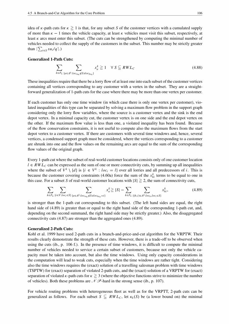
4.5 A Branch-and-Cut Algorithm for the Core Problem 106
idea of κ-path cuts for κ = 1 is that, for any subset S of the customer vertices with a cumulated supplyof more than κ − 1 times the vehicle capacity, at least κ vehicles must visit this subset, respectively, atleast κ arcs must enter this subset. (The cuts can be strengthened by computing the minimal number ofvehicles needed to collect the supply of the customers in the subset. This number may be strictly greaterthan d
∑i∈S sui /qe.)
Generalized 1-Path Cuts:∑k∈FL
∑{a∈Ak :loctaa 6∈S3lochea }
xka = 1 ∀ S j RW LC (4.88)
These inequalities require that there be a lorry flow of at least one into each subset of the customer verticescontaining all vertices corresponding to any customer with a vertex in the subset. They are a straight-forward generalization of 1-path cuts for the case where there may be more than one vertex per customer.
If each customer has only one time window (in which case there is only one vertex per customer), vio-lated inequalities of this type can be separated by solving a maximum flow problem in the support graphconsidering only the lorry flow variables, where the source is a customer vertex and the sink is the enddepot vertex. In a minimal capacity cut, the customer vertex is on one side and the end depot vertex onthe other. If the maximum flow value is less than one, a violated inequality has been found. Becauseof the flow conservation constraints, it is not useful to compute also the maximum flows from the startdepot vertex to a customer vertex. If there are customers with several time windows and, hence, severalvertices, a condensed support graph must be considered, where the vertices corresponding to a customerare shrunk into one and the flow values on the remaining arcs are equal to the sum of the correspondingflow values of the original graph.
Every 1-path cut where the subset of real-world customer locations consists only of one customer locationl ∈ RW LC can be expressed as the sum of one or more connectivity cuts, by summing up all inequalitieswhere the subset of V k
\ {d} is {i ∈ V k : loci = l} over all lorries and all predecessors of i . This isbecause the customer covering constraints (4.60a) force the sum of the xk
hi terms to be equal to one inthis case. For a subset S of real-world customer locations with |S| = 2, the sum of connectivity cuts,∑
k∈FL
∑{i∈V :loci∈S}
∑{a∈Ak :loctaa 6∈S3lochea=i}
xka = |S| −
∑k∈FL
∑{(h,i)∈Ak :loch ,loci∈S}
xkhi , (4.89)
is stronger than the 1-path cut corresponding to this subset. (The left hand sides are equal, the righthand side of (4.89) is greater than or equal to the right hand side of the corresponding 1-path cut, and,depending on the second summand, the right hand side may be strictly greater.) Also, the disaggregatedconnectivity cuts (4.87) are stronger than the aggregated ones (4.89).
Generalized 2-Path Cuts:Kohl et al. 1999 have used 2-path cuts in a branch-and-price-and-cut algorithm for the VRPTW. Theirresults clearly demonstrate the strength of these cuts. However, there is a trade-off to be observed whenusing the cuts (ib., p. 106 f.). In the presence of time windows, it is difficult to compute the minimalnumber of vehicles needed to service a certain subset of customers, because not only the vehicle ca-pacity must be taken into account, but also the time windows. Using only capacity considerations inthe computation will lead to weak cuts, especially when the time windows are rather tight. Consideringalso the time windows requires the (exact) solution of a travelling salesman problem with time windows(TSPTW) for (exact) separation of violated 2-path cuts, and the (exact) solution of a VRPTW for (exact)separation of violated κ-path cuts for κ = 3 (where the objective functions strive to minimize the numberof vehicles). Both these problems are N P-hard in the strong sense (ib., p. 107).
For vehicle routing problems with heterogeneous fleet as well as for the VRPTT, 2-path cuts can begeneralized as follows. For each subset S j RW LC , let κk(S) be (a lower bound on) the minimal
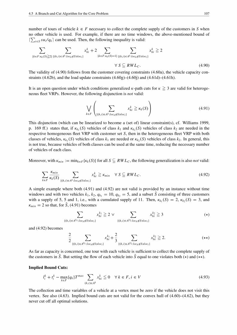
4.5 A Branch-and-Cut Algorithm for the Core Problem 107
number of tours of vehicle k ∈ F necessary to collect the complete supply of the customers in S whenno other vehicle is used. For example, if there are no time windows, the above-mentioned bound ofd∑
i∈S sui /qke can be used. Then, the following inequality is valid:∑{k∈F :κk (S)=2}
∑{(h,i)∈Ak :loch 6∈S3loci }
xkhi + 2
∑{k∈F :κk (S)=1}
∑{(h,i)∈Ak :loch 6∈S3loci }
xkhi = 2
∀ S j RW LC . (4.90)
The validity of (4.90) follows from the customer covering constraints (4.60a), the vehicle capacity con-straints (4.62b), and the load update constraints (4.60g)–(4.60j) and (4.61d)–(4.61h).
It is an open question under which conditions generalized κ-path cuts for κ = 3 are valid for heteroge-neous fleet VRPs. However, the following disjunction is not valid:
∨k∈F
∑{(h,i)∈Ak :loch 6∈S3loci }
xkhi = κk(S)
(4.91)
This disjunction (which can be linearized to become a (set of) linear constraint(s), cf. Williams 1999,p. 169 ff.) states that, if κk1(S) vehicles of class k1 and κk2(S) vehicles of class k2 are needed in therespective homogeneous fleet VRP with customer set S, then in the heterogeneous fleet VRP with bothclasses of vehicles, κk1(S) vehicles of class k1 are needed or κk2(S) vehicles of class k2. In general, thisis not true, because vehicles of both classes can be used at the same time, reducing the necessary numberof vehicles of each class.
Moreover, with κmin := mink∈F{κk(S)} for all S j RW LC , the following generalization is also not valid:
∑k∈F
κmin
κk(S)
∑{(h,i)∈Ak :loch 6∈S3loci }
xkhi = κmin ∀ S j RW LC . (4.92)
A simple example where both (4.91) and (4.92) are not valid is provided by an instance without timewindows and with two vehicles k1, k2, qk1 = 10, qk2 = 5, and a subset S consisting of three customerswith a supply of 5, 5 and 1, i.e., with a cumulated supply of 11. Then, κk1(S) = 2, κk2(S) = 3, andκmin = 2 so that, for S, (4.91) becomes∑
{(h,i)∈Ak1 :loch 6∈S3loci }
xk1hi = 2 ∨
∑{(h,i)∈Ak2 :loch 6∈S3loci }
xk2hi = 3 (∗)
and (4.92) becomes22
∑{(h,i)∈Ak1 :loch 6∈S3loci }
xk1hi +
23
∑{(h,i)∈Ak2 :loch 6∈S3loci }
xk2hi = 2. (∗∗)
As far as capacity is concerned, one tour with each vehicle is sufficient to collect the complete supply ofthe customers in S. But setting the flow of each vehicle into S equal to one violates both (∗) and (∗∗).
Implied Bound Cuts:
lki + tk
i −maxk∈F{qk}T max
∑(h,i)∈Ak
xkhi 5 0 ∀ k ∈ F, i ∈ V (4.93)
The collection and time variables of a vehicle at a vertex must be zero if the vehicle does not visit thisvertex. See also (4.63). Implied bound cuts are not valid for the convex hull of (4.60)–(4.62), but theynever cut off all optimal solutions.

4.6 Computational Experiments 108
Arrival Time Cuts:
tko − tk
d 5 0 ∀ k ∈ F (4.94)
The LP relaxation may initially yield a very bad lower bound, indeed, a negative one, because in a frac-tional solution, constraints (4.61i) allow that tk
d < tko for any vehicle k. The arrival time cuts prohibit
this. In any feasible solution, they must be fulfilled because of constraints (4.61a) (each vehicle reachesthe end depot vertex exactly once), the flow conservation constraints (4.61b), and the timing update con-straints (4.61i)–(4.61l).
No attempt was made to prove whether one of the above inequalities induces a facet for the VRPTTpolytope. Even for much simpler problems, polyhedral studies are extremely difficult. For example,Eglese/Letchford 2000, p. 217, call the polyhedron of the mixed rural postman problem ‘bewilderinglycomplicated’, and Naddef/Rinaldi 2002, p. 58, state that trying to prove facets for the symmetric capac-itated vehicle routing problem is ‘particularly hard’, and that the facial structure of the latter problem ‘isextremely complex and that there is still a lot to investigate in this field’ (ib., p. 71).
The above inequalities were considered as additional static or dynamic cuts in the branch-and-cut al-gorithm to strengthen the LP relaxation of (4.59)–(4.62). The supply collection cut, the trailer and thelorry flow cut and the implied bound and arrival time cuts were directly added to the formulation (staticcuts). The connectivity cuts and the generalized 1-path cuts were dynamically separated in the courseof the algorithm. Connectivity cuts were only separated when no violated 1-path cuts were found. Asfor the κ-path cuts, the computational experiments showed that, with and without them, only very smallinstances could be solved. Therefore, to find potentially violated κ-path cuts, all customer subsets wereenumerated, and each was tested as to whether there was a vehicle class of which at least two vehiclesare necessary to collect the supply of the customers in the subset. All relevant cuts were then added tothe formulation as static cuts.
4.5.2 Branching and Enumeration Strategies
The following three-stage branching strategy was used:
(i) branch on a lorry arc variable on the arc (o, d)
(ii) branch on a trailer arc variable entering a decoupling or leaving a coupling vertex
(iii) use the default CPLEX branching strategy (automatic selection of branching variable)
As enumeration strategy, the CPLEX default ‘best-bound’ strategy (select the vertex in the branch-and-bound tree with the best objective function value of the associated LP relaxation) was used.
4.6 Computational Experiments
The proposed branch-and-cut algorithm was implemented in C++ using the Boost Graph library andILOG Concert Technology.
4.6.1 Test Instances
In practice, the following types of vehicle are used:
• Collection vehicles:
– Single lorries:
∗ single lorry with two axles and a capacity of 10 tons∗ single lorry with three axles and a capacity of 15 tons

4.6 Computational Experiments 109
– Lorry-trailer combinations:
∗ two-axle lorry with two-axle trailer, both with a capacity of 10 tons (‘2/2-combination’)∗ two-axle lorry with three-axle trailer, with a capacity of 10 and 15 tons respectively
(‘2/3-combination’)∗ three-axle lorry with two-axle trailer, with a capacity of 15 and 10 tons respectively
(‘3/2-combination’)
• Support vehicles:
– two-axle lorry with three-axle trailer, with a capacity of zero and 25 tons respectively
The cost data used in the computational experiments are shown in Table 4.10. These data are realisticestimates, approximately reflecting absolute values of the different cost types for each vehicle type aswell as ratios of costs of one vehicle type to another. Two- and three-axle single lorries have the samecost data as two- and three-axle lorries of a lorry-trailer combination.
Cost type→Vehicle type ↓ Fixed Time-dependent Distance-dependent
Two-axle lorry 18,000 3,600 65Three-axle trailer 2,500 0 6Three-axle lorry 20,000 3,600 70Two-axle trailer 2,000 0 4
Table 4.10: Cost data for computational experiments
The customer and transshipment locations were randomly selected on a 100×100 km grid with the depotlocated in the centre. The resulting Euclidean distances between each pair of vertices were multipliedby a distance factor of 1.3. The customer supplies were chosen randomly from [1,000; 10,000]. Thetest instances were created with enough vehicles of each type such that the complete supply could becollected with one type of vehicle. For simplicity, support vehicles were not considered. As load transfertime, 2 minutes per 1,000 units of supply were assumed throughout.
The length of the planning horizon was assumed to be 12 hours or 1,320 minutes respectively. Allcustomers and pure transshipment locations have one time window: [0; 1,320]. For a code capable ofsolving problems with time windows, such instances represent the worst case. With tighter time win-dows, larger instances could be solved.
For each n ∈ {1, . . . , 10}, thirty so-called ‘x y z’ instances were created with the vehicle, cost and dis-tance data specified above. x stands for the number of lorry customers, y stands for the number of trailercustomers, and z stands for the number of pure transshipment locations, and x = y = z = n. This meansthat an x y z instance with nT S
= 3 has 1 + x + y + 3 · num trailers· (y + z) + 1 vertices: one for the
start depot, x for the lorry customers, y for the trailer customers, three for each combination of trailerand transshipment location (of which there are y + z) to represent decoupling, transfer, and coupling,and one for the end depot.
Some further deliberations on nT S , the number of transshipment processes per trailer and transshipmentlocation, follow. With nT S
= 3, there are no transshipment subtour symmetries, and no precedenceconstraints for the intermediate vertices to avoid such symmetries are necessary. However, if there areonly 2/3-combinations, and only lorry customers with identical supply of 5,001, then even nT S
= 4 isnot sufficient to guarantee that an optimal solution to the problem can be computed with formulation(4.59)–(4.62). With nT S
= 4, the following sequence of lorry and trailer loads results:

4.6 Computational Experiments 110
Transshipment operation 1 2 3 4Trailer load after operation 0 5,001 10,002 10,002Lorry load after operation 0 0 0 5,001
With nT S= 5, it is possible to visit one additional customer:
Transshipment operation 1 2 3 4 5Trailer load after operation 0 5,001 10,002 15,000 15,000Lorry load after operation 0 0 0 3 5,004
If there are only 3/2-combinations, a similar argument with lorry customer supplies of 7,501 yields thatnT S= 4 is sufficient. Hence, overall, with the above fleet data, it is sufficient to have nT S
= 5 forthree-axle trailers and nT S
= 4 for two-axle trailers to guarantee that an optimal solution obtained forthe formulation (4.59)–(4.62) is also an optimal solution to the underlying real-world problem instance.Nevertheless, the computational experiments were performed throughout with nT S
= 3 to keep thenetwork sizes limited.
4.6.2 System Parameters
The system parameters used in the computational experiments are shown in the following table. AllCPLEX parameters not shown in the table were at their default values. The selection of the algorithmfor solving the LP relaxations was left to CPLEX, the maximum flow problems for the separation of thesubtour elimination constraints were solved with the Edmonds-Karp algorithm provided by the BGL.
Parameter Setting
CPU frequency 2 GHzMain memory 1 GBCPLEX version 9.1Concert Technology version 2.1Wall-clock time limit 7,500 secondsMinimal violation of dynamic cutsto be considered violated 10−3
IloCplex::EpAGap 10−4
IloCplex::EpInt 10−4
IloCplex::CutLo −1075
IloCplex::EpGap 10−4
IloCplex::ObjDif 0IloCplex::RelObjDif 0IloCplex::CutUp 1075
Table 4.11: System parameters VRPTT
4.6.3 Computational Results
The following tables show the computational results obtained for the core formulation (4.59)–(4.62).
Table 4.12 shows how the size of the resulting mathematical programs develops for VRPTT instanceswith nT S
= 3 where all locations have one time window, and for VRPTW instances with the samenumber of customers. To compute the data in the table, it was assumed that the VRPTW networkconsists of one vertex per customer, one start, and one end depot vertex, one arc from the start depotvertex to all other vertices, and one arc from each customer vertex to each other customer vertex andthe end depot vertex. The number of vehicles in the VRPTW was assumed to be equal to the number of

4.6 Computational Experiments 111
lorries plus the number of trailers in the corresponding VRPTT. The number of constraints given in thetable was computed assuming an arc variable formulation with constraints for customer covering, flowconservation, update of resource variables and maintenance of static resource windows.
Instance type 1 1 1 2 2 2 2 2 2 3 3 3 4 4 4Vehicles 2 lorries 2 lorries 4 lorries 4 lorries 6 lorries
2 trailers 2 trailers 4 trailers 4 trailers 6 trailers
VRPTTVertices 16 30 54 80 154Arcs 131 493 1,477 3,283 11,737Arc variables 234 876 4,816 10,736 56,412Resource variables 92 168 496 728 1,920Constraints 910 3,378 18,989 42,250 223,504
VRPTWVertices 4 6 6 8 10Arcs 7 21 21 43 73Arc variables 28 84 168 344 876Resource variables 32 48 96 128 240Constraints 66 140 276 486 1,136
Table 4.12: VRPTT network size growth
Taking into account the number of variables and constraints as a measure for instance size, the 2 2 2and 3 3 3 instances, i.e., even instances with only 4 customers and 4 transshipment locations, can beconsidered large.
Table 4.13 shows the usefulness of the cuts described in Section 4.5.1. The table indicates the gap at theroot vertex of the branch-and-bound tree, i.e., the percentage by which the lower bound at the root vertexof the branch-and-bound tree (RL B) is below the best feasible solution as obtained with the branch-and-cut algorithm (B F S) for the different cut types: (B F S − RL B)/ B F S · 100. An entry of the formx / y / z in a row for cut c means that the RL B using only cut c was at least x % of B F S below B F S,was y % of B F S below B F S on average, and was at most z % of B F S below B F S. A value of 100corresponds to an RL B of zero, and a value greater than 100 corresponds to a negative RL B (which ispossible, see page 108). The trailer flow cut was not tested, because the test instances were created suchthat there is no customer with a supply exceeding the capacity of the largest lorry, and the number oflorries was always large enough to collect the complete supply of the customers without using a trailer,so that the number of necessary trailers is zero. Implied bound cuts were not tested, because CPLEXautomatically generates cuts where binary variables imply bounds on continuous variables. As indicatedin the previous section, the CPLEX cut generation routine was not turned off, so CPLEX automaticallyseparated several types of general (as opposed to problem-specific) cut.
Instance type 1 1 1 2 2 2 3 3 3 Average
Without time-dependent costsNo cuts 54 / 72 / 93 63 / 79 / 91 67 / 79 / 88 54 / 76 / 93Only supply collection cut 54 / 72 / 93 63 / 79 / 91 67 / 79 / 88 54 / 76 / 93Only lorry flow cut 8 / 21 / 41 25 / 39 / 60 30 / 33 / 38 8 / 31 / 60Only 2-path cuts 27 / 58 / 86 48 / 65 / 79 58 / 67 / 82 27 / 62 / 86Only arrival time cuts 54 / 72 / 93 63 / 79 / 91 67 / 79 / 88 54 / 76 / 93Only 1-path cuts 0 / 8 / 20 9 / 24 / 50 11 / 17 / 21 0 / 16 / 50Only connectivity cuts 32 / 44 / 59 38 / 55 / 72 41 / 49 / 52 32 / 49 / 72All cuts 0 / 2 / 13 0 / 8 / 18 10 / 12 / 15 0 / 5 / 18
(continued on next page)

4.6 Computational Experiments 112
(continued from previous page)Instance type 1 1 1 2 2 2 3 3 3 Average
With time-dependent costsNo cuts 133 / 164 / 196 82 / 129 / 174 134 / 139 / 148 82 / 146 / 196Only supply collection cut 133 / 164 / 196 81 / 129 / 174 134 / 139 / 148 81 / 146 / 196Only lorry flow cut 133 / 164 / 196 66 / 126 / 173 134 / 139 / 148 66 / 145 / 196Only 2-path cuts 124 / 160 / 193 70 / 120 / 171 122 / 130 / 143 70 / 140 / 193Only arrival time cuts 68 / 80 / 95 77 / 86 / 94 79 / 86 / 92 68 / 83 / 95Only 1-path cuts 126 / 161 / 196 63 / 119 / 161 122 / 129 / 136 63 / 140 / 196Only connectivity cuts 127 / 161 / 193 76 / 122 / 166 124 / 131 / 139 76 / 141 / 193All cuts 20 / 28 / 41 27 / 38 / 64 38 / 43 / 45 20 / 33 / 64
Table 4.13: Usefulness of cuts in VRPTT branch-and-cut algorithm (min. / avg. / max.)
The following observations can be made in Table 4.13:
• The application of all types of cut together significantly decreases the gap for both types of in-stance: For the instances without time-dependent costs, the average gap decreases from 76 % to5 %, for the instances with time-dependent costs, the average gap decreases from 146 % to 33 %.
• The application of all types of cut together clearly shows a synergy effect insofar as the gap isreduced considerably more than by the best type alone.
• The average gap for the instances without time-dependent costs is much smaller than that for theinstances with time-dependent costs.
• The cuts are much more useful for the instances without time-dependent costs, although the un-derlying polytope is the same as that for the instances with time-dependent costs. This suggeststhat, for the latter instances, the used inequalities cut off irrelevant parts of the feasible region ofthe LP relaxation, or rather that the objective function decreases in the ‘wrong’ direction.
• The supply collection cut is not useful.
• The arrival time cuts are not useful for the instances without time-dependent costs, but for theinstances with time-dependent costs, they are the strongest type of cut.
• Each other type of cut is useful for the instances without time-dependent costs, but not for theinstances with time-dependent costs unless all types of cut are applied together.
Table 4.14 shows the computational results obtained with the branch-and-cut algorithm. The meaning ofthe row ‘% Gap at end’ is the same as in Chapter 3: It indicates the percentage by which the best feasiblesolution (B F S) exceeds the best lower bound at the end of the optimization (BL B) (it is zero if anoptimal solution is found, and it is not counted if no feasible solution is found): (B F S−BL B)/ BL B·100.
Instance type 1 1 1 2 2 2 3 3 3 Average
Without time-dependent costsNo. of tried / feasible / optimal 30 / 30 / 30 30 / 30 / 28 30 / 7 / 6 30 / 22 / 21Running time [s] 0 / 1 / 3 18 / 1,141 / 7,500 473 / 3,211 / 7,500 0 / 847 / 7,500% Gap at end 0 / 0 / 0 0 / 1 / 18 0 / 0 / 1 0 / 0 / 18No. of B&B vertices 1 / 3 / 11 10 / 222 / 846 124 / 1,141 / 3,085 1 / 220 / 3,085No. of separated 1-path cuts 1 / 11 / 33 102 / 270 / 837 432 / 882 / 1,462 1 / 218 / 1,462No. of separated conn. cuts 0 / 15 / 78 59 / 514 / 1,974 201 / 1,862 / 3,076 0 / 431 / 3,076No. of lorry tours 1 / 1.0 / 1 1 / 1.3 / 2 1 / 1.0 / 1 1 / 1.1 / 2No. of trailer tours 0 / 0.3 / 1 1 / 1.0 / 2 1 / 1.0 / 1 0 / 0.7 / 2
(continued on next page)

4.7 Conclusions 113
(continued from previous page)Instance type 1 1 1 2 2 2 3 3 3 Average
With time-dependent costsNo. of tried / feasible / optimal 30 / 30 / 30 30 / 30 / 0 5 / 4 / 0 22 / 21 / 10Running time [s] 1 / 4 / 11 7,500 / 7,500 / 7,500 7,500 / 7,500 / 7,500 1 / 3,931 / 7,500% Gap at end 0 / 0 / 0 0 / 43 / 178 45 / 58 / 62 0 / 23 / 178No. of B&B vertices 28 / 155 / 442 172 / 6,359 / 12,230 722 / 1,445 / 1,812 28 / 3,093 / 12,230No. of separated 1-path cuts 19 / 47 / 84 514 / 2,261 / 3,975 1,535 / 2,367 / 2,931 19 / 1,214 / 3,975No. of separated conn. cuts 41 / 92 / 178 661 / 1,975 / 4,036 2,695 / 4,050 / 5,411 41 / 1,210 / 5,411No. of lorry tours 1 / 1.0 / 1 1 / 1.4 / 4 1 / 1.0 / 1 1 / 1.2 / 4No. of trailer tours 0 / 0.3 / 1 0 / 1.0 / 2 1 / 1.0 / 1 0 / 0.7 / 2
Table 4.14: Computational results for VRPTT (min. / avg. / max.)
Three 4 4 4 instances without time-dependent costs were also tried, but for none of them could a feasiblesolution be computed within the time limit.
The following observations can be made in Table 4.14:
• Only instances with a very small number of customers and transshipment locations can be solved.This is mainly due to the fact that the size of the resulting mathematical programs grows sharplywith increasing number of (trailer) customers, transshipment locations, and vehicles. See Table4.12.
• The difficulty of the instances, or rather, the difficulty that the algorithm has with different in-stances of the same type and size (as indicated by the running times), varies widely.
• The number of vertices in the branch-and-bound trees is quite high.
• It is remarkable that instances with time-dependent costs are so much harder to solve than instanceswithout.
The largest instances that can consistently be solved to optimality are 2 2 2 instances (4 customers,4 transshipment locations) with 8 vehicles, 4,800 binary variables, and 19,000 constraints, and 3 3 3instances (6 customers, 6 transshipment locations) with 4 vehicles, 1,900 binary variables, and 7,400constraints. Tests have shown that a direct solution of such instances by submitting only the formula-tion (4.59)–(4.62) to CPLEX is impossible. For example, the instance 2 2 2 0 (4 vehicles, 870 binaryvariables, 3,300 constraints) without time costs took more than 15,000 seconds to solve and had 244,000vertices in the branch-and-bound tree with CPLEX alone; with the branch-and-cut algorithm, it took 93seconds to solve and had 70 vertices in the branch-and-bound tree. The instance 2 2 2 1 (8 vehicles,4,800 binary variables, 19,000 constraints) without time costs had a gap of more than 80 % after morethan 15,000 seconds with CPLEX alone; with the branch-and-cut algorithm, it was solved in less than1,500 seconds.
4.7 Conclusions
This chapter has considered the vehicle routing problem with trailers and transshipments. In this prob-lem, the vehicle fleet consists of autonomous vehicles (lorries) able to move on their own, and of non-autonomous vehicles (trailers) which must be accompanied by an autonomous vehicle to be able to move.Moreover, both autonomous and non-autonomous vehicles are either collection or support vehicles. Thedecisive aspects of the problem are the consideration of trailers which can be pulled by different lorries,of support vehicles unable to visit customers, and of load transfers between arbitrary vehicles. Theseaspects lead to very complex interdependencies between the vehicles. Considering the complexity of thecomplete problem, a ‘core’ problem has been extracted capturing only central aspects of a free lorry-trailer assignment.
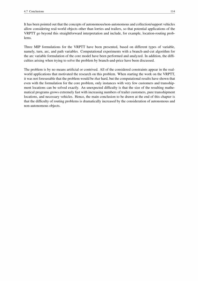
4.7 Conclusions 114
It has been pointed out that the concepts of autonomous/non-autonomous and collection/support vehiclesallow considering real-world objects other than lorries and trailers, so that potential applications of theVRPTT go beyond this straightforward interpretation and include, for example, location-routing prob-lems.
Three MIP formulations for the VRPTT have been presented, based on different types of variable,namely, turn, arc, and path variables. Computational experiments with a branch-and-cut algorithm forthe arc variable formulation of the core model have been performed and analyzed. In addition, the diffi-culties arising when trying to solve the problem by branch-and-price have been discussed.
The problem is by no means artificial or contrived. All of the considered constraints appear in the real-world applications that motivated the research on this problem. When starting the work on the VRPTT,it was not foreseeable that the problem would be that hard, but the computational results have shown thateven with the formulation for the core problem, only instances with very few customers and transship-ment locations can be solved exactly. An unexpected difficulty is that the size of the resulting mathe-matical programs grows extremely fast with increasing numbers of trailer customers, pure transshipmentlocations, and necessary vehicles. Hence, the main conclusion to be drawn at the end of this chapter isthat the difficulty of routing problems is dramatically increased by the consideration of autonomous andnon-autonomous objects.

Chapter 5
The Truck-and-Trailer Routing Problem
The truck-and-trailer routing problem (TTRP) is a special case of the VRPTT, where there is a fixedassignment of a lorry to a trailer (and vice versa), i.e., each trailer may be pulled by only one lorry, andonly this lorry may perform a load transfer into this trailer. Consequently, there are no support vehicles.
The chapter is structured as follows. In the next section, the differences between the TTRP and the coreVRPTT are pointed out, and two new MIP formulations for the TTRP, based on arc and path variablesrespectively, are developed. In Sections 5.2 and 5.3, a branch-and-cut and a branch-and-price algorithmfor the TTRP are presented. The results of computational experiments with these two algorithms arepresented and analyzed in Section 5.4. The chapter ends with a short conclusion.
5.1 New MIP Formulations for the TTRP
5.1.1 Assumptions
The TTRP as considered here is a special case of the core VRPTT. The additional assumptions made inthis chapter are as follows:
• Due to the fixed lorry-trailer assignment, the vehicles considered in the TTRP are either singlelorries (as in a ‘usual’ VRP) or lorry-trailer combinations (LTCs). As before, the vehicles maydiffer with respect to (fixed, distance- and time-dependent) costs and capacity, and there may alsobe accessibility constraints for particular vehicles at some locations. For LTCs, two capacities arerelevant: the lorry capacity and the trailer capacity. The sum of these capacities is the overallvehicle capacity of an LTC. An LTC lorry need not use its trailer and may simply leave it at thedepot. If a trailer is used, it cannot be left behind at a transshipment location by its lorry, it mustalso be pulled back to the depot.
Single lorry
.......................................................................................................................................................................... .....................................................................................................................................................................................
........
........
........
........
........
........
........
....................................................................................................................................................................................................................................................................................................... ......................................
.......
Jointed lorry-trailer combination (LTC)
LTC lorry
.....................................................................................................................................................................................................................................................................................................................................................................................
........
........
........
........
........
........
........
....................................................................................................................................................................................................................................................................................................... ......................................
.......
Trailer
............................................................................................................................................................................................................................................................................................................................................................................................................................................................................................................................................................................................. ......................................
....... ...................................................................................
.......
Figure 5.1: TTRP fleet
• All customers and all transshipment locations have only one time window.
Figure 5.2 depicts a possible route plan with one single lorry and one LTC. The single lorry route is evi-dent. The LTC lorry starts at the depot with its trailer, visits a trailer customer, goes on to a transshipmentlocation, decouples the trailer, visits two customers, returns to the transshipment location, re-couples the
115

5.1 New MIP Formulations for the TTRP 116
trailer, pulls it to a second transshipment location, decouples it again (and perhaps performs a load trans-fer), visits two more customers, returns to the second transshipment location, re-couples the trailer andreturns to the depot. Two transshipment locations in the centre of the figure are not used. The reader maycompare this figure with Figure 4.2.
.................................................
..................................... ppppppppppppppppppppppppppppppppppppppppppppppppppppppppppppppppppppppppppppppppppppppppppppppppppppppppppppppppppppppppppppppppppppppppppppppppppppppppppppppppppppppppppppppppppppppppppppppppppppppppppppppppppppppppppppppppppppppppppppppppppppppppppppppppppppppppppppppppppppppppppppppppppppppppppppppppppppppppppppppppppppppppppppppppppppppppppppppppppppppppp ....................................................................................................
.............
.............
.............
.............
.............
.............
............ ..........................
......................... ............pppppppppppppppppppppppppppppppppppppppppppppppppppppppppppppppppppppppppppppppppppppppppppppppppppppppppppppppppppppppppppppppppppppppppppppppppppppppppppppppppppppppppppppppp pppppppppppp ........
.....
........
.....
........
.....
................
............
..........................
..........................
............. ............ ............
...............................................................pppppppppppppppppppppppppppppppppppppppppppppppppppppppppppppppppppppppppppppp pppppppppppp................................................................................................................................................................................................................................................ ............ .........................................................................................
..............
.........................................................................................................................................................................................................
......................................................................................................................................................................................................................................................................................................
............................
............................
.............................................
..........................................
.......................................... .............................................................
.......................................................................................................................... ............ ............
........................
........................
.......................................
N
N
uuuu
uu uuu
�
�
�
�
�
��
� �
�
Depot
Lorry customer
Trailer customer
Transshipment location
Single lorry
LTC lorry
LTC
Figure 5.2: Example of a TTRP route plan
5.1.2 Underlying Network
The subsequent formulation is based on a time-space-operation network D = (V, A) which is a simpli-fied version of the time-space-operation-vehicle network of Section 4.3.3.2 for the VRPTT. The notationused in this chapter is the same as in the previous one unless otherwise specified. RW L:={Depot} ·∪RW LC ·∪ RW LT is the set of relevant real-world locations. As before, RW LC := RW LCL
·∪ RW LCLT .Each vertex in V corresponds to a location in space, an absolute and/or relative period of time, and a typeof operation. For each customer, there is one vertex. The decisive difference between the two networksis that, in the TTRP network, the transshipment vertices are not trailer-specific: The set of transship-ment vertices, VIT , now contains only one subset {vdecouple
l , vtrans f er,1l , . . . , vtrans f er,nT S
−2l , vcouple
l } for eachtransshipment location l, i.e., the number of possible transshipment operations is now assumed to beindependent of the trailer, respectively, the LTC class, and of the location. This is possible because of thefixed lorry-trailer assignment: When a lorry visits a decoupling, transfer, or coupling vertex, it is clearwhich trailer is decoupled, to which trailer a load transfer is performed, and which trailer is coupled. Ifan LTC wants to use transshipment location l, the LTC must first visit vdecouple
l . The trailer then moves intime to the vertices vtrans f er,1
l , . . . , vtrans f er,nT S−2
l , vcouplel , while the LTC lorry visits customers and finally
re-couples the trailer at vcouplel . The LTC lorry need not visit any of the transfer vertices of l. The LTC
lorry must not visit any other vertex in VIT before having re-coupled its trailer at vcouplel . The formulation
below takes this into account.
All vehicles are initially at the start depot vertex o and end their tour at the end depot vertex d. Singlelorries are allowed, in principle, to visit lorry and trailer customer vertices, and LTC lorries may, in prin-ciple, visit all vertices of D. Trailers can only reach the transshipment vertices and the trailer customers.
It is assumed that each LTC uses each transshipment location at most once. Thus, for each trailer, thereare at most nT S transshipment operations at each transshipment location. The deliberations on the ‘cor-rect’ choice of nT S in the chapter on the VRPTT apply here, too. However, in the branch-and-pricealgorithm, the numerical value of nT S need not be fixed in advance; rather, this value is determined dur-ing the solution of the pricing problems.

5.1 New MIP Formulations for the TTRP 117
The arc set consists of the following arcs:
• (o, d)
• (o, vc) and (vc, d) for all customer vertices vc ∈ VC
• (o, vdecouplel ) for all transshipment locations l ∈ RW LCLT
·∪ RW LT
• (vcouplel , d) for all transshipment locations l ∈ RW LCLT
·∪ RW LT
• (vc, vc′) for all customer vertices vc, vc′ ∈ VC with c 6= c′
• (vdecouplel , vc) for all transshipment locations l ∈ RW LCLT
·∪ RW LT and all customer verticesvc ∈ VC
• (vtrans f er,il , vc) for all transshipment locations l ∈ RW LCLT
·∪ RW LT , all i ∈ {1, . . . , nT S−2} and
all customer vertices vc ∈ VC
• (vcouplel , j) for all transshipment locations l ∈ RW LCLT
·∪ RW LT and all vertices j ∈ (Vdecouple \
{vdecouplel }) ·∪ VCLT
• (i, j) for all trailer customer vertices i ∈ VCLT and all transshipment vertices j ∈ VIT
• (i, j) for all lorry customer vertices i ∈ VCL and all transfer and coupling vertices j ∈ Vtrans f er·∪ Vcouple
Figure 5.3 visualizes the subnetworks for the different vehicle types. As in the corresponding figurefor the core VRPTT, there is only one arc for each arc type present in the subnetwork of the respectivevehicle type. Tables 5.1, 5.2, and 5.3 also give an overview of the arcs in A.
0 1 2 3 4 5 6start depot lorry c. trailer c. decoupling transfer coupling end depot
0 start depot – X X – – – X1 lorry c. – X X – – – X2 trailer c. – X X – – – X3 decoupling – – – – – – –4 transfer – – – – – – –5 coupling – – – – – – –6 end depot – – – – – – –
Table 5.1: Single lorry arcs in TTRP
0 1 2 3 4 5 6start depot lorry c. trailer c. decoupling transfer coupling end depot
0 start depot – X X X – – X1 lorry c. – X X – X X X2 trailer c. – X X X X X X3 decoupling – X X – – – –4 transfer – X X – – – –5 coupling – – X X – – X6 end depot – – – – – – –
Table 5.2: LTC lorry arcs in TTRP

5.1 New MIP Formulations for the TTRP 118
N N
u u
� �
� � �
� � �o d
Lorry customers
Trailer customers
Decouple Trans-fer
Couple ppppppppppppppppppppppppppppppppppppppppppppppppppppppppppppppppppppppppppppppppppppppppppppppppppppppppppppppppppppppppppppppppppppppppppppppppppppppppppppppppppppppppppppppppppppppppppppp pppppppppppppppppppppppppppppppppppppppppppppppppppppppppppppppppppppppppppppppppppppppppppppppppppppppppppppppppppppppppppppppppppppppppppppppppppppppppppppppppppppppppppppppppppppppppppppppppppppppppppppppppppppppppppppp pppppppppppp pppppppppppppppppppppppppppppppppppppppppppppppppppppppppppppppppppppppppppppppppppppppppppppppppppppppppppppppppppppppppppppppppppppppppppppppppppppppppppppppppppppppppppppp pppppppppppp ppppppppppppppppppppppppppppppppppppppppppppppppppppppppppppppppppppppppppppppppppppppppppppppppppppppppppppppppppppppppppppppppppppppppppppppppppppppppppppppppppppppppppppppppppppppppppppppppppppppppppppppp pppppppppppppppppppppppppppppppppppppppppppppppppppppppppppppppppppppp pppppppppppp
pppppppppppppppppppppppppppppppppppppppppppppppppppppppppppppppppppppppppppppppppppppppppppppppppppppppppppppppppppppppppppppppp ppppppppppppppppppppppppppppppppppppppppppppppppppppppppppppppppppppppppppppppppppppppppppppppppppppppppppppppppppppppppppppppppppppppppppppppppppppppppppppppppppppppppppppppppppppppppppppp ppppppppppppN N
� �
� �
� �o d
Lorry customers
Trailer customers
Decouple Couple
Network vertices Subnetwork for LTCs
............................................................................................... ............................................................................................... ......................
....................
....................
...........................................
............................................................................................... ..................................
......................
.................................
............ ............................................................................ ............
...........................................................................
........
........
........
........
........
...................
............
........
........
........
........
........
........
........
..............
...........................................................................
...............
............................................................................................................................................................................................................................... ..................
................................................................................................................................................
..................
..................
..................
.....
................ ........
....
...............................u u
� �
� � �
� � �
Lorry customers
Trailer customers
Decouple Trans-fer
Couple ..............................
..............................
..............................
..............................
..............................
..............................
..............................
..........................
....................................................................................................................................................................................................................... ............
............................................................................................... ............
............................................................................................. ............
............................................................................................................................................................................................................................ ............
..................................
..................................
..................................
..................................
..................................
.............................................
............
............................................................................................................................................................................................................................... ..................
................................................................................................................................................
..................
..................
..................
.....
................ ........
....
...............................
N N
u u
� �
o d
Lorry customers
Trailer customers
Subnetwork for LTC lorries Subnetwork for single lorries and LTC lorrieswhen trailer is at transshipment location when trailer is not used
Figure 5.3: TTRP subnetworks
0 1 2 3 4 5 6start depot lorry c. trailer c. decoupling transfer coupling end depot
0 start depot – – X X – – X1 lorry c. – – – – – – –2 trailer c. – – X X – – X3 decoupling – – – – (X) (X) –4 transfer – – – – (X) (X) –5 coupling – – X X – – X6 end depot – – – – – – –
Table 5.3: Trailer arcs in TTRP
F := FL ·∪ FLT denotes the set of vehicles. FL is the set of single lorries, which do not have a trailer.FLT is the set of lorry-trailer combinations. Ak
LT :=Ak\({(i, j) ∈ A : i ∈ VCL
·∪ Vdecouple} ·∪ {(i ′, j ′) ∈A : j ′ ∈ VCL
·∪ Vcouple} ) is the set of arcs LTC lorry k can traverse with its trailer attached. clorr y,ki j
denotes the costs of traversing arc (i, j) with lorry k ∈ F (for LTC lorries, without the trailer attached),and ctrailer,k
i j denotes the additional costs of pulling LTC lorry k’s trailer over arc (i, j). On arcs (o, j)emanating from the start depot o, except for the arc (o, d), the fixed vehicle costs are included in clorr y,k
oj ,respectively, ctrailer,k
oj . For all k ∈ F , q totalk is the total capacity of a vehicle, i.e., it is the capacity of
single lorry k, or the capacity of LTC lorry k and its trailer respectively. For all k ∈ FLT , q lorr yk is the
capacity of LTC lorry k, and q trailerk is the capacity of LTC lorry k’s trailer.

5.1 New MIP Formulations for the TTRP 119
5.1.3 A Formulation Based on Arc Variables
There are the following variables:
• xki j ∈ {0, 1} ∀ k ∈ F, (i, j) ∈ Ak .
xki j =
{1, lorry k traverses arc (i, j)0, otherwise
• yki j ∈ {0, 1} ∀ k ∈ FLT , (i, j) ∈ Ak
LT .
yki j =
{1, trailer k traverses arc (i, j)0, otherwise
• lcoll,ki ∈ R0
+∀ k ∈ F, i ∈ V k .
The total amount of customer supplies that lorry k has collected when reaching vertex i , before kstarts its service at i .
• l trans,ki ∈ R0
+∀ k ∈ FLT , i ∈ V k .
The total amount of customer supplies that LTC lorry k has transferred to its trailer when reachingvertex i , or, equivalently, the load of LTC lorry k’s trailer when k reaches vertex i (with or withoutits trailer attached), before k starts its service at i .
• tki ∈ R0
+∀ k ∈ F, i ∈ V k .
The point in time when lorry k starts its service at vertex i .
The resulting formulation is:
(TTRP):∑k∈F
∑(i, j)∈Ak
clorr y,ki j xk
i j +∑
k∈FLT
∑(i, j)∈Ak
LT
ctrailer,ki j yk
i j +∑k∈F
ctimek (tk
d − tko )→ min (5.1)
subject to∑k∈F
∑(h,i)∈Ak
xkhi = 1 ∀ i ∈ VC (5.2a)
∑(h,i)∈Ak
xkhi 5 1 ∀ k ∈ FLT , i ∈ Vdecouple (5.3a)
∑(vcouple
l , j)∈AkLT
xkvcouple
l j−
∑(h,vdecouple
l )∈AkLT
xkhvdecouple
l= 0 ∀ k ∈ FLT , l ∈ RW LCLT
·∪ RW LT (5.3b)
∑(h,i)∈Ak
xkhi −
∑(vcouple
l , j)∈AkLT
xkvcouple
l j5 0 ∀ k ∈ FLT , l ∈ RW LCLT
·∪ RW LT , i ∈ Vtrans f er ,
loci = l (5.3c)∑(i,d)∈Ak
xkid = 1 ∀ k ∈ F (5.3d)
∑(i,d)∈Ak
LT
ykid = 1 ∀ k ∈ FLT (5.3e)
∑(h,i)∈Ak
xkhi −
∑(i, j)∈Ak
xki j = 0 ∀ k ∈ F, i ∈ V k
\ {o, d} (5.3f)

5.1 New MIP Formulations for the TTRP 120
∑(h,i)∈Ak
LT
ykhi −
∑(i, j)∈Ak
LT
yki j = 0 ∀ k ∈ FLT , i ∈ V k
CLT(5.3g)
yki j 5 xk
i j ∀ k ∈ FLT , (i, j) ∈ AkLT \ {(o, d)}, i 6∈ Vcouple,
j 6∈ Vdecouple (5.3h)
xkhi = yk
hi ∀ k ∈ FLT , i ∈ Vdecouple, (h, i) ∈ AkLT (5.3i)
xki j = yk
i j ∀ k ∈ FLT , i ∈ Vcouple, (i, j) ∈ AkLT (5.3j)
l trans,ki 5 lcoll,k
i ∀ k ∈ FLT , i ∈ V k (5.4a)
lcoll,ki − l trans,k
i 5 q lorr yk ∀ k ∈ FLT , i ∈ V k (5.4b)
xki j = 1⇒ lcoll,k
i + sui 5 lcoll,kj ∀ k ∈ F, (i, j) ∈ Ak (5.4c)
xki j = 1⇒ l trans,k
i 5 l trans,kj ∀ k ∈ FLT , (i, j) ∈ Ak (5.4d)
xki j = 1⇒ l trans,k
i = l trans,kj ∀ k ∈ FLT , i ∈ VCL , (i, j) ∈ Ak (5.4e)
xki j = 1 ∧ yk
i j = 0⇒ l trans,kj 5 l trans,k
i ∀ k ∈ FLT , i ∈ VCLT , (i, j) ∈ Ak (5.4f)
yki j = 1⇒ l trans,k
j 5 l trans,ki + sui ∀ k ∈ FLT , i ∈ VCLT , (i, j) ∈ Ak
LT (5.4g)
xki j = 1⇒ tk
i + τ tri j 5 tk
j ∀ k ∈ F, i ∈ {o} ·∪ VC , (i, j) ∈ Ak (5.4h)
xki j = 1⇒ tk
i + (l trans,kj − l trans,k
i )τ lt+ τ tr
i j 5 tkj ∀ k ∈ FLT , i ∈ VIT , (i, j) ∈ Ak (5.4i)
tkvdecouple
l− tk
vtrans f er,1l
5 0 ∀ k ∈ FLT , l ∈ RW LCLT·∪ RW LT (5.4j)
tkvtrans f er,i
l− tk
vtrans f er,i+1l
5 0 ∀ k ∈ FLT , i ∈ {1, . . . , nT S− 3},
l ∈ RW LCLT·∪ RW LT (5.4k)
tk
vtrans f er,nT S−2l
− tkvcouple
l5 0 ∀ k ∈ FLT , l ∈ RW LCLT
·∪ RW LT (5.4l)
tkvcouple
l− T
∑(h,vdecouple
l )∈AkLT
xkhvdecouple
l5 0 ∀ k ∈ FLT , l ∈ RW LCLT
·∪ RW LT (5.4m)
xki j ∈ {0, 1} ∀ k ∈ F, (i, j) ∈ Ak (5.5a)
yki j ∈ {0, 1} ∀ k ∈ FLT , (i, j) ∈ Ak
LT (5.5b)
0 5 lcoll,ki 5 q total
k ∀ k ∈ F, i ∈ V k (5.5c)
0 5 l trans,ki 5 q trailer
k ∀ k ∈ FLT , i ∈ V k (5.5d)
twai 5 tki 5 twbi ∀ k ∈ F, i ∈ V k (5.5e)

5.1 New MIP Formulations for the TTRP 121
(5.1) is the objective function, which minimizes total costs. Constraints (5.2) are logical coupling con-straints, (5.3) are non-coupling flow constraints, (5.4) are non-coupling constraints specifying the updateof the resource variables, and (5.5) determine the ranges of the variables.
(5.2a) are the customer covering constraints. Each customer must be visited exactly once.
(5.3a)–(5.3c) make sure that each transshipment location is used at most once by each k ∈ FLT , andthat only intermediate and coupling vertices of those transshipment locations are used whose decouplingvertex is visited.
(5.3d) and (5.3e) require that each vehicle reach the end depot (perhaps via the arc (o, d)).
(5.3f) and (5.3g) are flow conservation constraints.
(5.3h)–(5.3j) are the constraints linking the routing of the trailer to that of its lorry. Note that it is possiblethat an LTC lorry does not use its trailer, in which case the latter moves directly from o to d.
(5.4a) requires that the load of the trailer be at most equal to the total amount of supply collected. With-out this constraint, l trans,k
i can always be set to the trailer capacity. Because of constraint (5.4b), lcoll,ki is
then bounded from above by the overall vehicle capacity, and not by the lorry capacity and the amountof load actually transferred. This effectively enlarges the lorry capacity. A lorry can then park its trailerbefore doing any collecting and can collect as much supply as the overall vehicle capacity permits, with-out having to transfer any load.
(5.4c) are the load update constraints. The total amount of load collected increases (at least) by the sup-ply of each vertex visited.
Similarly, constraints (5.4d)–(5.4g) are for the update of the transshipment variables, respectively, thetrailer load variables. (5.4d) states that the trailer load is non-decreasing. (5.4e) states that the trailerload is non-increasing at lorry customer vertices. (5.4f) states that at trailer customer vertices, the trailerload of an LTC lorry k can only increase if the vertex is visited by k and its trailer. (5.4g) states that, at atrailer customer vertex, the trailer load does not increase by more than the customer’s supply.
Constraints (5.4h)–(5.4i) are the constraints for the update of the timing variables.
(5.4j)–(5.4m) are needed to make sure that the vertices of a transshipment location are visited in the cor-rect order, i.e., that decoupling vertices of a transshipment location are visited before their correspondingcoupling vertex. Without this constraint, it would be possible to visit decoupling vertex vdecouple
l1 , go tocoupling vertex vcouple
l2 , then to decoupling vertex vdecouplel2 and then to vcouple
l1 . Moreover, these constraintsavoid transshipment subtour symmetries (cf. p. 85) if there is more than one transfer vertex per location,i.e., if nT S = 4. If an LTC lorry does not visit a transshipment intermediate vertex for some l, the timevariables for these vertices can be fixed appropriately; it is not required to have a visiting time of zero fornon-visited vertices. In principle, it is also possible to set nT S
= 2. Then, (5.4j)–(5.4l) must be replacedby
tkvdecouple
l− tk
vcouplel
5 0 ∀ k ∈ FLT , l ∈ RW LT ·∪ RW LCLT . (5.6)
(5.4m) serves the same purpose as (5.3b) and (5.3c). Hence, when (5.3b) and (5.3c) are used, (5.4m) isredundant, and vice versa.

5.1 New MIP Formulations for the TTRP 122
Note that there are no constraints limiting the total tour duration other than the length of the planninghorizon.
An alternative choice of variables is to use a (binary) resource variable yki indicating whether LTC lorry k
reaches vertex i with or without its trailer attached. This leads to fewer variables and to fewer constraints(5.4g), but to more and more complicated constraints (5.3g).
Instead of the two resource variables concerning the load, it is also possible to consider variables spec-ifying the current load of the lorry and, if applicable, its trailer. In this case, constraints (5.4a) are notnecessary, but constraints (5.4b) have to be replaced by
l trailer,kj 5 l trailer,k
i + llorr y,ki + sui ∀ k ∈ FLT , (i, j) ∈ Ak, (5.7)
i.e., there are more constraints than with the above choice of variables (unless time window or capacityrestrictions are extremely tight).
The above formulation differs from the TTRP as described in Chao 2002 and formulated in Scheuerer2004 in the following aspects:
• The above papers consider no variable costs for the trailers, no fixed costs for the vehicles, and notime-dependent costs at all (Chao 2002, p. 34, Scheuerer 2004, p. 43).
• The above papers consider only the trailer customer locations and the depot as possible transship-ment locations (Chao 2002, p. 34, Scheuerer 2004, p. 45). In the network used in this chapter,it is also possible to have transshipment vertices corresponding to other real-world locations. Thedepot is not explicitly considered as a transshipment location, but it can trivially be added to theset of possible transshipment locations. However, this does not really make sense. At the depot,no load transfer from lorry to trailer is performed, but any load a vehicle carries will be unloaded,and any vehicle leaving the depot will be empty. Hence, the load of a lorry and its trailer mustbe reset to zero after a ‘transshipment’ operation at the depot. This means that having the depotas a possible transshipment location amounts to allowing multiple use of vehicles, but this is notconsidered for simplicity.
• Scheuerer 2004 (p. 45) does not allow that several lorry-trailer combinations use the same trans-shipment location.
• The above papers do not consider time windows.
• The above papers assume that a transshipment operation takes a fixed amount of time, independentof the amount of load transferred (Scheuerer 2004, p. 51).
The only existing formulations for the TTRP, by Semet 1995 and Scheuerer 2004, are conceptually dif-ferent from the above formulation. Scheuerer 2004 uses binary three-index arc variables similar to theabove yk
i j variables, and five-index variables indicating whether a certain lorry traverses a certain arcon the nth subtour starting at a certain trailer customer or at the depot, where n is the number of cus-tomers. (In the worst case, as many single lorry (sub-)tours starting at a trailer customer or at the depotare necessary as there are customers.) Semet 1995 uses similar variables, but requires that at most onesubtour originate at each trailer customer, so that the second variable type has only four indices in hisformulation. Neither author uses resource variables, but rather, both formulations are pure 0-1 IPs.
A weakness of (5.1)–(5.5) compared to the formulations presented by Semet 1995 and Scheuerer 2004lies in the fact that, in order to linearize the implications in several constraints of (5.1)–(5.5), largeconstants M must be introduced, which makes for a weak LP relaxation of (5.1)–(5.5). The formulationsby Semet 1995 and Scheuerer 2004 do not use such constants. A potential advantage of (5.1)–(5.5)compared to the formulation by Scheuerer 2004 lies in constraints (5.4j)–(5.4l), as Scheuerer 2004 doesnot include any constraints for breaking transshipment subtour symmetries.

5.1 New MIP Formulations for the TTRP 123
5.1.4 A Formulation Based on Path Variables
This section presents a path variable reformulation of (5.1)–(5.5). For simplicity, and to avoid difficultiesin the solution of the pricing problems as for the VRPTT, the following simplifications are made:
(i) The time-dependent costs in the objective function are disregarded.
(ii) The load transfer times at transshipment vertices are assumed to be fixed, independent of theamount of load transferred.
If fixed load transfer times for the TTRP are assumed, it is possible to consider time windows, a maximaltour duration and time costs in a labelling algorithm with the standard resource concept as described inChapter 2 for the solution of the pricing problems. (If time-dependent costs and fixed load transfer timesare considered, but no time windows, the time-dependent costs can be put entirely on the arcs, togetherwith the distance-dependent costs, as no waiting occurs. In the presence of time windows, however,waiting may occur, and if there are time-dependent costs, the total waiting time must be minimized. Thiscould be done as described in Desaulniers/Villeneuve 2000, cf. p. 100.) However, the TTRP, as consid-ered in Chao 2002 and Scheuerer 2004, considers neither time costs nor time windows, and almost allpapers on VRPs consider no time-dependent costs.
Fixed load transfer times are an alternative well worth considering. A little solution precision gets lost,but it is to be expected that larger instances can be solved. If this simplification is made, it is arguablethat it also makes sense not to consider the trailer routing costs, because they are quite low comparedto the lorry costs (in reality and in the instances used in the computational experiments). However,the consideration of the exact trailer costs does not make the solution any more difficult, so it is betterto consider this aspect of the problem correctly. To consider fixed load transfer times in (5.1)–(5.5),constraints (5.4h) and (5.4i) are replaced by
xki j = 1⇒ tk
i + τ tri j 5 tk
j ∀ k ∈ F, (i, j) ∈ Ak (5.8)
The usual decomposition approach for VRPs can then also be applied to the TTRP. The logical couplingconstraints, i.e., the customer covering constraints (5.2), define the master program, the non-couplingconstraints (5.3)–(5.5) define the sub- or pricing problems.
5.1.4.1 The Master Program
As for VRPs without trailers and for the VRPTT, each feasible tour of a single lorry in the TTRP is anelementary path from the start depot vertex to the end depot vertex through the respective subnetwork.This is also true for the LTC lorries. However, the movements of a trailer in the network D of Section5.1.3 do not constitute a path: There are no trailer flow variables leaving decoupling vertices or enteringcoupling vertices. This, though, is only to avoid unnecessary variables and constraints. In the real world,the itinerary of a single lorry or a trailer resulting from a solution to (5.1)–(5.5) is an elementary path,too, whereas the itinerary of an LTC lorry using its trailer is not necessarily elementary; it may containcycles starting and ending at the transshipment locations where the trailer is parked.
It follows from the flow decomposition theorem (cf. Ahuja et al. 1993, p. 80 f.) that the extreme pointsof the convex hull of all points fulfilling the pricing problems’ constraints (5.3)–(5.5) correspond to lorrypaths from o to d in D, some of which may be non-elementary, because D is not acyclic. For LTCs, con-straints (5.3d)–(5.3j) additionally imply that the extreme points represent a path-like structure consistingof an o-d-path for the lorry and one or more paths for its trailer. The union of these trailer paths is asubset of the lorry path.

5.1 New MIP Formulations for the TTRP 124
These extreme points are described by flow and resource vectors
(xkp, yk
p, lcoll,kp , l trans,k
p , tkp) = (xk
i j p, yki j p, lcoll,k
ip , l trans,kip , tk
ip)
∀ k ∈ F, p ∈ Pk, (i, j) ∈ Ak, (5.9)
where Pk is the set of extreme points for single lorry or LTC k. For simplicity of notation, in (5.9) andin the following, it is assumed that
yki j = yk
i j p = ykp = ctrailer,k
i j := 0 ∀ k ∈ FL ,and
l trans,ki = l trans,k
ip = l trans,kp := 0 ∀ k ∈ FL .
Any solution satisfying (5.3)–(5.5) can be expressed as a convex combination of these extreme points:
xki j =
∑p∈Pk
xki j pλ
kp ∀ k ∈ F, (i, j) ∈ Ak (5.9a)
xki j ∈ {0, 1} ∀ k ∈ F, (i, j) ∈ Ak (5.9b)
yki j =
∑p∈Pk
yki j pλ
kp ∀ k ∈ FLT , (i, j) ∈ Ak
LT (5.9c)
yki j ∈ {0, 1} ∀ k ∈ FLT , (i, j) ∈ Ak
LT (5.9d)
lcoll,ki =
∑p∈Pk
lcoll,kip λk
p ∀ k ∈ F, i ∈ V k (5.9e)
l trans,ki =
∑p∈Pk
l trans,kip λk
p ∀ k ∈ FLT , i ∈ V k (5.9f)
tki =
∑p∈Pk
tkipλ
kp ∀ k ∈ F, i ∈ V k (5.9g)
∑p∈Pk
λkp 5 1 ∀ k ∈ F (5.9h)
λkp = 0 ∀ k ∈ F, p ∈ Pk (5.9i)
The integer master program (IMP) is then:
∑k∈F
∑p∈Pk
∑(i, j)∈Ak
clorr y,ki j xk
i j p
λkp +
∑k∈FLT
∑p∈Pk
∑(i, j)∈Ak
LT
ctrailer,ki j yk
i j p
λkp → min (5.10)
subject to
∑k∈FL
∑p∈Pk
∑i∈V l
C
∑(h,i)∈Ak
xkhip
λkp = 1 ∀ l ∈ RW LC (5.11a)
∑p∈Pk
λkp 5 1 ∀ k ∈ F (5.11b)
λkp = 0 ∀ k ∈ F, p ∈ Pk (5.11c)
λkp ∈ {0, 1} ∀ k ∈ F, p ∈ Pk (5.11d)

5.1 New MIP Formulations for the TTRP 125
In general, it is not true that binary restrictions on the original xki j arc variables can be replaced by binary
restrictions on the λkp path variables. However, this statement holds for the above TTRP reformulation,
since the definition of the original master problem solution space, i.e., the constraint set (5.2), involvesonly the xk
i j variables. Hence, binary requirements on the path variables are equivalent to binary require-ments on the xk
i j variables, cf. Desaulniers et al. 1998, p. 75. Moreover, if the xki j variables are binary,
the yki j variables will be binary, too. This is because, for any path of an LTC lorry k represented by the
values of the xki j variables, the values of the pertinent yk
i j variables are unequivocally determined: If thepath visits transshipment vertices, all partial paths ending at a decoupling vertex or starting at a couplingvertex have all yk
i j variables equal to one, and all partial paths between a decoupling and its correspond-ing coupling vertex have all yk
i j variables equal to zero. Paths visiting only customers and at least onelorry customer have all yk
i j variables equal to zero, and paths visiting only trailer customers have all yki j
variables equal to one, unless the total demand of the customers on the path does not exceed the lorrycapacity, in which case the corresponding trailer will not be used.
5.1.4.2 The Pricing Problems
The pricing problems’ constraints are (5.3)–(5.5). The objective functions for single lorries and LTCscan be derived as follows:
Introducing dual variables
(α, γ ) := (α1, . . . , α|RW LC |, γ 1, . . . , γ |F |) (5.12)
for constraints (5.11a) and (5.11b), the reduced costs of a path p are
ckp(α, γ ) =
∑(i, j)∈Ak
clorr y,ki j xk
i j p +∑
(i, j)∈AkLT
ctrailer,ki j yk
i j p −∑
l∈RW LC
∑i∈V l
C
∑(h,i)∈A
xkhip
αl− γ k . (5.13)
The reduced costs of the arcs in the pricing problem for a vehicle k can be stated as in Table 5.4.
cki j for
clorr y,ki j − αl (i, j) 6∈ Ak
LT , j ∈ V kC , locj = l
clorr y,ki j + ctrailer,k
i j δtrailer,ki j − αl (i, j) ∈ Ak
LT , j ∈ V kCLT
, locj = l
clorr y,ki j + ctrailer,k
i j j ∈ Vdecouple
clorr y,ki j j ∈ Vtrans f er ·∪ Vcouple
clorr y,kid + ctrailer,k
id − γ k j = d
Table 5.4: Reduced costs for arcs in the TTRP pricing problem for vehicle k
δtrailer,ki j fulfils
δtrailer,ki j =
{1, k ∈ FLT and k traverses (i, j) with its trailer attached0, otherwise
∀ k ∈ F, (i, j) ∈ Ak .
The branch-and-price algorithm described in Section 5.3 uses a resource to correctly consider the ctrailer,ki j
in the solution of the LTC pricing problems.
The objective function of the pricing problem for vehicle k can be written as∑(i, j)∈Ak
clorr y,ki j xk
i j +∑
(i, j)∈AkLT
ctrailer,ki j yk
i j −∑
l∈RW LC
∑i∈V l
C
∑(h,i)∈Ak
αl xkhi − γ k . (5.14)
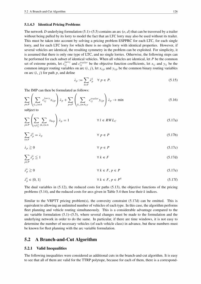
5.2 A Branch-and-Cut Algorithm 126
5.1.4.3 Identical Pricing Problems
The network D underlying formulation (5.1)–(5.5) contains an arc (o, d) that can be traversed by a trailerwithout being pulled by its lorry to model the fact that an LTC lorry may also be used without its trailer.This must be taken into account by solving a pricing problem ESPPRC for each LTC, for each singlelorry, and for each LTC lorry for which there is no single lorry with identical properties. However, ifseveral vehicles are identical, the resulting symmetry in the problem can be exploited. For simplicity, itis assumed that there is only one type of LTC, and no single lorries. Otherwise, the following steps canbe performed for each subset of identical vehicles. When all vehicles are identical, let P be the commonset of extreme points, let clorr y
i j and ctraileri j be the objective function coefficients, let xi j and yi j be the
common integer routing variables on arc (i, j), let xi j p and yi j p be the common binary routing variableson arc (i, j) for path p, and define
λp :=∑k∈F
λkp ∀ p ∈ P. (5.15)
The IMP can then be formulated as follows:∑p∈P
∑(i, j)∈A
clorr yi j xi j p
λp +∑p∈P
∑(i, j)∈ALT
ctraileri j yi j p
λp → min (5.16)
subject to∑p∈P
∑i∈V l
C
∑(h,i)∈A
xhip
λp = 1 ∀ l ∈ RW LC (5.17a)
∑k∈F
λkp = λp ∀ p ∈ P (5.17b)
λp = 0 ∀ p ∈ P (5.17c)∑p∈P
λkp 5 1 ∀ k ∈ F (5.17d)
λkp = 0 ∀ k ∈ F, p ∈ P (5.17e)
λkp ∈ {0, 1} ∀ k ∈ F, p ∈ Pk (5.17f)
The dual variables in (5.12), the reduced costs for paths (5.13), the objective functions of the pricingproblems (5.14), and the reduced costs for arcs given in Table 5.4 then lose their k indices.
Similar to the VRPTT pricing problem(s), the convexity constraint (5.17d) can be omitted. This isequivalent to allowing an unlimited number of vehicles of each type. In this case, the algorithm performsfleet planning and vehicle routing simultaneously. This is a considerable advantage compared to thearc variable formulation (5.1)–(5.5), where several changes must be made to the formulation and theunderlying network in order to do the same. In particular, if there are time windows, it is not easy todetermine the number of necessary vehicles (of each vehicle class) in advance, but these numbers mustbe known for fleet planning with the arc variable formulation.
5.2 A Branch-and-Cut Algorithm
5.2.1 Valid Inequalities
The following inequalities were considered as additional cuts in the branch-and-cut algorithm. It is easyto see that all of them are valid for the TTRP polytope, because for each of them, there is a correspond-

5.2 A Branch-and-Cut Algorithm 127
ing valid inequality for the VRPTT. Although the TTRP polytope differs from the VRPTT polytope, thearguments presented in the section on valid inequalities for the VRPTT can be applied here analogously.Hence, the inequalities are restated only because of small logical and notational differences.
Supply Collection Cut: ∑k∈F
lcoll,kd =
∑l∈RW LC
csl (5.18)
Trailer Flow Cut: ∑k∈FLT
∑{(i,d)∈Ak :i 6=o}
ykid = num trailers (5.19)
A lower bound for num trailers can be computed as for the VRPTT trailer flow cut, with sutrailer definedas
sutrailer=
∑l∈RW LC
csl −∑k∈F
q lorr yk . (5.20)
Lorry Flow Cut: ∑k∈F
∑{(i,d)∈Ak :i 6=o}
xkid = numlorries (5.21)
The minimal number of necessary lorries, numlorries , can be computed by sorting all vehicles by non-increasing total capacity (including trailer capacity) and summing up the total vehicle capacities, startingwith a biggest vehicle, until the sum exceeds the total customer supply. For each lorry that contributes tothe sum, numlorries must be increased by one.
Connectivity Cuts: ∑{a∈Ak :taa 6∈S∪{i},hea∈S}
xka − xk
hi = 0 ∀ k ∈ F, S j V k\ {d}, (h, i) ∈ Ak, h ∈ S (5.22)
Generalized 1-Path Cuts:∑k∈F
∑{(h,i)∈Ak :loch 6∈S3loci }
xkhi = 1 ∀ S j RW LC (5.23)
Generalized 2-Path Cuts:For the TTRP, using the information that there is a fixed lorry-trailer assignment, (4.90) can be strength-ened to∑
k∈FL
1κk(S)
∑{(h,i)∈Ak :loch 6∈S3loci }
xkhi
+
∑k∈FLT
1κk(S)
∑{(h,i)∈Ak :loch 6∈S3loci }
(xkhi − yk
hi )
+
∑k∈FLT
1κ ′k(S)
∑{(h,i)∈Ak :loch 6∈S3loci }
ykhi = 1 ∀ S j RW LC , (5.24)
where, for each k ∈ F , κk(S) is (a lower bound on) the minimal number of lorry tours necessary to collectthe complete supply of the customers in S when no other vehicle is used and κk(S) := min{2, κk(S)},and where, for each k ∈ FLT , κ ′k(S) is (a lower bound on) the minimal number of LTC tours necessary tocollect the complete supply of the customers in S if no other vehicle is used, and κ ′k(S) := min{2, κ ′k(S)}.

5.3 A Branch-and-Price Algorithm 128
Implied Bound Cuts:
lcoll,ki + tk
i −maxk∈F{q total
k }T∑
(h,i)∈Ak
xkhi 5 0 ∀ k ∈ F, i ∈ V (5.25)
For transshipment vertices i , the tki summand must be left out because of (5.4k)–(5.5a).
Arrival Time Cuts:
tko − tk
d 5 0 ∀ k ∈ F (5.26)
5.2.2 Branching and Enumeration Strategies
Two branching strategies were tried:
(i) a five-stage strategy going from global to local branching criteria as follows:
• branch on the number of tours
• branch on an arc with fractional total flow, i.e., where the total number of lorries traversingthat arc is fractional. If possible, use an arc whose tail or head is a customer vertex, whoseflow value is between 0.4 and 0.6, and whose length is maximal. Otherwise, use the first arcwith non-integer flow.
• branch on a lorry arc variable on the arc (o, d)
• branch on a trailer arc variable entering a decoupling or leaving a coupling vertex
• branch on a variable close to 0.5 having high absolute objective function coefficient
It did not prove useful to also use the ‘close to 0.5 and high objective function coefficient’ strategyfor the choice of the lorry or trailer flow variable.
(ii) a three-stage strategy using only the last three, the ‘local’, stages of the five-stage strategy
Preliminary computational experiments showed that the three-stage strategy consistently outperformedthe five-stage strategy with respect to running time. The number of subproblems and the number ofsolved LPs were significantly lower than with the five-stage strategy, but the highest level reached inthe branch-and-bound tree was higher with the three-stage strategy. This may be partially caused by thefact that branching on the number of tours is not too useful for arc variable formulations, as there is astrong correlation between minimal total distance covered and minimal number of vehicles used. Thisis all the more so if fixed vehicle costs are considered, as was the case in the computational experimentsperformed. Consequently, Section 5.4 shows the computational results obtained with the three-stagestrategy.
As enumeration strategy, ‘dive and best’ was used. This strategy performs depth-first search until afeasible solution is found, and then performs best-first search.
5.3 A Branch-and-Price Algorithm
5.3.1 The Pricing Problems
5.3.1.1 Literature Review
As mentioned in the previous chapter, there is a considerable amount of literature on the solution of(E)SPPRCs as pricing problems in branch-and-price approaches for VRP(TW)s and related problems.A brief review of important contributions follows. All cited papers solve the (E)SPPRCs by a labellingalgorithm.

5.3 A Branch-and-Price Algorithm 129
Until fairly recently, most approaches for solving VRP(TW)s by branch-and-price solved only the non-elementary SPPRC in the pricing step (see, for example, Kohl et al. 1999). Due to the negative cycles,non-elementary Pareto-optimal o-d-paths may exist. Columns corresponding to such paths may be use-ful during the solution process (cf. Desrosiers/Lubbecke 2005, p.12), but these columns can never bepart of a feasible solution to the VRP(TW), so they must be eliminated in the branching process.
2-cycles, i.e., negative cycles consisting of two antiparallel arcs, are encountered very often. In labellingalgorithms, they can be eliminated with comparatively little computational overhead. The basic ideais to keep at a vertex i only one Pareto-optimal label l1 and one ‘second-best’ label l2 with a differentpredecessor vertex. If a label l3 resident at i dominates neither l1 nor l2, i.e., if l3’s consumption of eachresource is greater than or equal to the corresponding consumption of both l1 and l2, l3 can be discarded.
Irnich/Villeneuve 2006 describe κ-cycle elimination for cycles containing κ = 3 arcs. (This means thatall cycles containing κ or fewer arcs are eliminated.) Their approach has been very successfully used(see, e.g., Fukasawa et al. 2006), but it is very involved and cannot be described here.
Feillet et al. 2004 have performed computational experiments with a branch-and-price approach for theVRPTW, where they solved the ESPPRC using visitation counter resources as described in Section 2.3.These experiments show the following: There is a trade-off between solving the SPPRC and the ESP-PRC. The former problem is much easier to solve (by several orders of magnitude), but the resultinglower bounds for the master problem are very weak, even when using 2-cycle elimination. The latterproblem provides very good lower bounds, but direct solution of the elementary problem can be pro-hibitively difficult. This is mostly due to the fact that the dominance procedure is very weak whenvisitation counters are used.
The approaches by Chabrier 2006, Boland et al. 2006, and Salani 2005 try to find a compromise bydeferring or even completely avoiding the use of all visitation counters while still solving the elementaryversion of the problem. To this end, the problem is solved iteratively. Chabrier 2006 solves the ESP-PRC by not extending a path to an already visited vertex, while ignoring the visitation counters in thedominance procedure for partial paths comprising less than a certain number n of arcs. In the course ofthe algorithm, n is adjusted (decreased) until a negative reduced cost path is found or n = 0, in whichcase the visitation counters are considered for all paths. While n > 0, the ESPPRC is not solved exactly,because not necessarily all undominated negative reduced cost paths will be returned; it is possible thata path is dominated by another path although both cover different customers. The dominated path couldpossibly have been extended to a customer the dominating path has already visited, and such an exten-sion could lead to a negative reduced cost path which now will not be discovered. Boland et al. 2006(see also Salani 2005) use the concept of incremental state space augmentation. First, they solve theSPPRC without any visitation counters. (The state space of the dynamic-programming-based labellingalgorithm consists only of the space defined by the ‘usual’ resources like cost, time, and capacity.) Ifnon-elementary paths are returned, so-called critical vertices are determined. These are vertices that arevisited more than once in at least one of the returned paths. For the critical vertices, visitation countersare introduced and the problem is solved again. (The state space is incremented by the space defined bythe added visitation counters.) This process is repeated until only elementary paths are returned.
In the worst case, none of the last three approaches can avoid solving the ESPPRC on the complete statespace if the VRP(TW) is to be solved exactly.
The above approaches perform so-called heuristic pricing before the exact solution of the elementaryproblem. There are numerous other approaches for generating negative reduced cost columns withoutsolving the ESPPRC exactly. These include (cf. Ropke 2005, p. 202 ff.)
• solving the problem on a reduced network by considering at each vertex only the k shortest ema-nating arcs,

5.3 A Branch-and-Price Algorithm 130
• limiting the (overall) number of labels that may exist at any point in time in the course of thealgorithm,
• solving the SPPRC, examining the resulting paths for negative cycles, and removing them, and
• creating paths by a construction heuristic or by modifying existing paths via local search.
Salani 2005 successfully applies bounded bidirectional labelling algorithms to solve the ESPPRC. Thebasic idea of bidirectional labelling algorithms is to keep the number of labels as low as possible bysimultaneously (forward-)extending towards d partial paths starting at o and (backward-)extending to-wards o partial paths ‘starting’ at d, and to stop the procedure as soon as forward and backward labelscan be joined to yield an o-d-path. Bidirectional labelling is not a heuristic in itself; it is an alternativelabelling algorithm technique. It can be applied in any of the approaches just described (cycle elimina-tion, state space augmentation etc.). Whether it solves the underlying problem exactly or not depends onthe REFs and the dominance procedure.
Bidirectional labelling algorithms have already been used for solving the SPP (Ahuja et al. 1993, p. 112f.). Applying the principle to solve the ESPPRC is somewhat more involved. The REFs for forwardextension of labels are essentially the same as in the unidirectional algorithm. The REFs for backwardextension are, in principle, analogous to the forward REFs. However, their definition and implementa-tion (at least for the TTRP with its intricate interdependencies between trailer positions, collected andtransferred load) is quite complicated and laborious.
Three additional steps are necessary or at least highly recommendable in a bidirectional labelling algo-rithm compared to an unidirectional one (Salani 2005, p. 31 ff.):
(i) To avoid creating every path twice, once by forward and once by backward extension, boundingof extensions must be performed.To this end, a cardinally scaled and constrained so-called critical resource is selected. This re-source must have a non-negative consumption along all arcs. A forward or backward label isextended only if the consumption of the critical resource in the label resulting from the extensionis not more than half of the upper resource window bound at d.
(ii) A join operation of a forward and a backward label is required to yield an o-d-path.To this end, when all forward and backward extension steps are performed, the forward labels ateach vertex i are joined with all backward labels at all vertices j for which an arc from i to j exists.The overall resource consumptions of the resulting o-d-paths are computed, and the feasible pathsare returned (when they have negative reduced costs).
(iii) Uniqueness of solutions should be ensured.Contrary to most situations in optimization, where it is sufficient to find only one (feasible oroptimal) solution, in the pricing problems in column generation, it is sensible to store several orall solutions with negative reduced cost (also structurally different solutions with the same costs).This means that it is not sensible to keep only one negative reduced cost path. However, evenwhen bounding is applied, paths may be generated more than once. If a negative reduced costpath contains a sequence of three vertices i , j , and k (in this order), the path may be generatedby a join of the forward path from o to i and the backward path from d to j as well as by a joinof the forward path from o to j and the backward path from d to k. Such duplicate paths cannotbe discarded on the basis of costs alone, and checking whether two paths with the same negativereduced costs are structurally different can be computationally expensive (a comparison of the pathstructure of two paths cannot be done in constant time). Thus, to ensure uniqueness of solutions inconstant time, a so-called half-way test can be performed. A feasible join of a forward path fromo to i and a backward path from d to j is performed only when the following two conditions aremet: (i) The consumption of the critical resource on both the forward and the backward path is

5.3 A Branch-and-Price Algorithm 131
not more than half of the overall consumption of the resource along the complete path (along thisparticular path; for any feasible path, this will always be less than or equal to half of the upperresource window of the critical resource at d), and (ii) the consumption on the forward path plusthe consumption on the arc (i, j) is at least half of the overall consumption of the resource alongthe complete path. To make this point clear, consider the following example. If the consumptionof the critical resource at d must not be more than 100, and if there is a feasible, negative reducedcost path (o, a1, i, a2, j, a3, k, a4, d) with an overall consumption of the critical resource of 40,then without the half-way test, this path would be generated four times, through joins via each ofthe four arcs. If the consumption of the critical resource is 15 at i and 25 at j (i.e., the consumptionalong a2 is 10), the half-way test will join the two partial paths (o, a1, i) and (d, a4, k, a3, j) viaarc a2, and will discard all other joins.
5.3.1.2 Strategies for the Solution of the Pricing Problems
Taking the results of the above authors into account, the following seven strategies for the solution of thepricing problems were tried:
(i) Solution of SPPRCs for all vehicles with two-cycle elimination.
(ii) Solution of ESPPRCs in one stage, i.e., using visitation counters for all customers in the extensionand in the dominance step.
(iii) Solution of ESPPRCs in two stages. In the first stage, the visitation counters were used only inthe extension step, but not in the dominance step. In the second stage, the visitation counters wereused in both steps.
(iv) Solution of ESPPRCs in three stages. The first stage consisted in solving the ESPPRCs on reducednetworks containing only the κ shortest arcs emanating from any vertex. For instances with upto 15 customer vertices, κ was set to 3; for larger instances, it was set to 5. As in the first stageof (iii), the visitation counters were used only in the extension step, but not in the dominancestep. In the second stage, the ESPPRCs were solved on the full network, considering all visitationcounters in the extension step, and considering only the visitation counters for customers whosecovering constraints in the master problem had a high dual price (who were covered in the currentmaster problem solution by an artificial variable) in the dominance step. In the third stage, thevisitation counters for all customers were considered in both the extension and the dominance step.Additionally, in the second and the third stage, only labels were extended that could possibly stilllead to labels with negative reduced costs at the end depot vertex. To this end, the lowest reducedcosts on any arc entering a customer vertex and the lowest reduced costs on any arc entering theend depot vertex were determined. In the extension step, the former costs were multiplied withthe maximum number of customers that could still be visited (considering capacity and time).Together with the latter costs, this product was added to the current label costs, and the extensionwas deemed infeasible if the sum was non-negative. Experiments showed that this bounding-by-reduced-costs procedure improved the solution speed by approximately three percent compared toa three-stage approach without bounding.
(v) Solution of ESPPRCs in three stages. In the first and second stage, the visitation counters wereused only in the extension step, but not in the dominance step. In the first stage, the ESPPRCswere solved on a reduced network as in (iv). In the second stage, the ESPPRCs were solvedon the full networks. The third stage consisted in solving the ESPPRCs on the full networks byincremental state space augmentation, where in each iteration, all customer vertices correspondingto customers visited more than once were added to the set of critical vertices.
(vi) Solution of ESPPRCs in three stages as in (iv), but for the second and third stage, the boundedbidirectional labelling algorithm was applied. The collected load was selected as the critical re-source. At intermediate vertices, the increase in the collected load is zero. Therefore, to guarantee
5.3 A Branch-and-Price Algorithm 132
uniqueness of the solutions, an additional join test was used: A join of a forward and a backwardlabel was only performed if the end vertex of the path corresponding to the forward label was acustomer vertex.
(vii) Heuristic solution of the ESPPRCs by only performing the first and second stage of (v). By skip-ping the third stage, the ESPPRCs are not solved exactly, and the complete branch-and-price algo-rithm becomes a heuristic. (This is similar to the heuristic labelling algorithm of Chapter 3.)
In strategies (iii)–(vii), a stage s > 1 was performed only when all stages s ′ < s did not return any nega-tive reduced cost paths for any vehicle (class). The pricing routine always tried to find negative reducedcost paths for all vehicles (vehicle classes) before returning, no matter whether negative reduced costpaths had already been found for one or more vehicles (vehicle classes) or not. In this way, emphasiswas put on quickly returning many negative reduced cost columns. So-called partial pricing, i.e., notsolving the (E)SPPRC for all vehicles (vehicle classes), but returning as soon as a negative reduced costpath for one vehicle (class) is found (cf. Irnich 2002, p. 97 f.) was also tried, but did not yield betterresults.
In addition, the discretization approach described in Section 4.3.5 was implemented for the TTRP. Thisyielded large acyclic networks with task cycles. (The networks themselves do not contain cycles, so thateach vertex is visited at most once, but it is possible to visit more than one vertex corresponding to oneand the same customer.) So, the problem of negative cycles remains. The discretization approach alsodid not work well. In the experiments, all computation times were much longer than with the cyclicnetwork (by one order of magnitude).
The 2-cycle elimination strategy (i) proved unusable, because the lower bounds were much too weak,so that huge branch-and-bound trees were built up. The one- and two-stage ESPPRC strategies (ii) and(iii) were not as fast as the three-stage strategy (iv). Therefore, in Section 5.4, computational results arereported only for strategies (iv)–(vii).
5.3.1.3 Resources and Resource Extension Functions
The resources used in the labelling algorithm for vehicle k are:
• an unconstrained, cardinally scaled resource for cost
• one cardinally scaled resource for each of the three resource variables used in (5.1)–(5.5), i.e., forcollected load, transferred load, and time
• a cardinally scaled visitation counter resource for each customer
• two nominally scaled auxiliary resources for LTC trailers
In the following, these resources are described in detail. The auxiliary resources are presented first, be-cause they are needed to describe the REFs for cost and load.
The first auxiliary resource is needed for the correct modelling of the routing logic at transshipmentlocations. It must be considered that, on its itinerary, an LTC lorry must visit the decoupling, transfer,and coupling vertices of each transshipment location in the correct order (or not at all), and that, after anLTC lorry has visited the decoupling vertex of transshipment location l, it must not visit any decoupling,transfer, or coupling vertex of any other transshipment location before having visited the coupling vertexof l. To this end, two types of constraint are needed: so-called pairing-and-precedence constraints andfollower constraints, see Irnich/Desaulniers 2005, p. 39 f. These authors also present REFs for suchconstraints (ib., p. 44 f.). They give a possible REF for pairing-and-precedence constraints and an REFfor follower constraints. Each REF requires one extra resource. However, it is possible to use only onenominally scaled resource r tp (and one REF) to model the trailer logic. r tp (‘trailer position’) records

5.3 A Branch-and-Price Algorithm 133
the current position of the trailer by means of a resource variable σtpi , which indicates the position of the
trailer when the LTC lorry reaches vertex i . σtpi is either zero, meaning that the LTC lorry is currently
pulling its trailer, or equal to the vertex number of the decoupling vertex where the trailer was parked.The corresponding REF is f r tp
with
f r tp
i j (σtpi ) =
σ
tpi , j ∈ VC ·∪ Vtrans f er ·∪ {d}j, j ∈ Vdecouple
0, j ∈ Vcouple
, (5.27)
and the resource windows at a vertex j are as shown in Table 5.5.
Resource window for{0} j ∈ {o, d} ·∪ Vdecouple
{1, . . . , |V |} j ∈ VCL
{0, . . . , |V |} j ∈ VCLT
{i} j ∈ Vtrans f er ·∪ Vcouple, i ∈ Vdecouple, locj = loci
Table 5.5: Resource windows for r tp at vertex j
r tp is also needed to model the load transfer logic at trailer customer and transshipment locations, andfor the update of the visitation counter resources.
Moreover, r tp does not only determine the feasibility of an extension of a path along an arc, it is relevantfor dominance considerations, too: A label can only dominate another label if their respective currenttrailer positions are equal.
To consider the reduced costs of the arcs in the pricing problems for LTCs, the second additional resource,r y , is needed to express the yk
i j variables. r y is a binary resource. Its value equals one, if LTC lorry kreaches i with its trailer attached, and equals zero otherwise. The corresponding resource variable is σ
yi ,
and the REF is f r ywith
f r y
i j (σy
i , σtpi ) =
{1, (σ
tpi = 0 ∧ i 6∈ Vdecouple) ∨ i ∈ Vcouple
0, otherwise. (5.28)
For each of the resource variables used in formulation (5.1)–(5.5), there is one constrained resource. Forthe total amount of customer supplies that lorry k has collected when reaching vertex i , the resource r coll
with resource variable σ colli and REF f rcoll
with
f rcoll
i j (σ colli ) = σ coll
i + sui (5.29)
was used. f rcoll
i j models constraints (5.4c) and sets σ collj to the lowest nonnegative value fulfilling these
constraints. The resource window at a vertex j is [0, q totalk ].
For the total amount of customer supplies that LTC lorry k has transferred when reaching vertex i , theresource r trans with resource variable σ trans
i and REF f r transwith
f r trans
i j (σ transi , σ coll
i , σtpi ) =
σ transi , j ∈ VCL ∨ ( j ∈ VCLT ∧ σ
tpi 6= i)
σ transi +min{sui , q trailer
k − σ transi } , j ∈ VCLT ∧ σ
tpi = i
σ transi +min{σ coll
i − σ transi , q trailer
k − σ transi }, j ∈ VIT
(5.30)
was used. f r trans
i j models constraints (5.4a), (5.4b), and (5.4d)–(5.4g) and sets σ transj to the highest possi-
ble value that fulfils these constraints. The resource window at a vertex j is [0, q trailerk ].

5.3 A Branch-and-Price Algorithm 134
This means that an LTC lorry always transfers as much load as possible to its trailer (its complete loador an amount of load equal to the residual capacity of its trailer, whichever is less). This is a sensiblestipulation, as it was assumed above that the time needed for a load transfer is fixed, independent of theactual amount of load transferred.
For the point in time when lorry k begins its service at vertex i , the resource r time with resource variableσ time
i and REF f r timewith
f r time
i j (σ timei ) = max
{twaj , σ
timei + τ tr
i j
}(5.31)
was used. f r time
i j models constraints (5.8) and sets σ timej to the lowest nonnegative value fulfilling these
constraints. The resource window at a vertex j is [twaj , twbj ].
For each vc ∈ VC , there is one visitation counter resource r visi t,vc with resource variable σ vci at each
vertex i ∈ V and REF f rvisi t,vc with
f rvisi t,vc
i j (σ vci , σ coll
j , σ transj , σ time
j , σtpj ) =
{0 , vc = i ∨ not enough capacity ∨ not enough timeσ vc
i , otherwise(5.32)
where σ vcj = 0 means that customer vc cannot be visited any more, and where ‘not enough capacity’
means
σ collj + su j > q total
k
∨ (vc 6= j ∧ σ collj + su j + suvc > q total
k )
∨ (σtpj 6= j ∧ σ coll
j − σ transj + su j > q lorr y
k )
∨ (vc 6= j ∧ σtpj 6= j ∧ σ coll
j − σ transj + su j + suvc > q lorr y
k )
and ‘not enough time’ means
σ timej + τ tr
jvc> twbvc , where τ tr
hh := 0 ∀ h ∈ V .
The resource window for vertex j at vertex j is [1, 1], and the resource window for a vertex j ′ 6= j atvertex j is [0, 1].
As explained in Section 5.1.3, transshipment subtour symmetries are possible if there is more than oneintermediate vertex per transshipment location. Such symmetries are excluded in formulation (5.1)–(5.5)by constraints (5.4j)–(5.4l). However, when the pricing problems are solved by a labelling algorithm, itis not necessary to introduce more than one intermediate vertex in the LTC subnetworks. (It is optimalto choose nT S
= 3.) It is sufficient to have only one, and to allow multiple visits to this vertex. Visitationcounters are maintained only for the customers, not for the transshipment vertices. With one intermediatevertex, no transshipment subtour symmetries are possible. Also, elementarity of paths can be ensuredwith visitation counters only for the customers, as every possible cycle in the subnetworks (as well as inthe network corresponding to the arc variable formulation) contains a customer. It is then also possible touse a transshipment location more than once, which can be relevant if there are time windows. This is anadditional degree of freedom that constitutes a considerable advantage of the path variable formulationcompared to the arc variable formulation.
Indeed, when the pricing problems are solved by a labelling algorithm, it is sufficient to use only onevertex per transshipment location. Although this reduces the subnetwork size for the LTC subproblems,the number of possible labels, which determines the difficulty of an (E)SPPRC, remains the same.
Finally, there is one unconstrained resource r cost measuring the costs. The corresponding resource vari-able is σ cost
i , and the REF for single lorries and LTC lorries that do not use their trailer is f rcostwith

5.3 A Branch-and-Price Algorithm 135
f rcost
i j (σ costi ) = σ cost
i + cki j , (5.33)
where cki j are the reduced costs of traversal of arc (i, j) for vehicle k. The REF for LTCs is
f rcost
i j (σ costi , σ
yj ) = σ cost
i + cki j (σ
yj ), (5.34)
where cki j (σ
yj ) are the reduced costs of traversal of arc (i, j) for LTC k. σ
yj is needed to carry the infor-
mation whether the LTC lorry is currently pulling its trailer, so that the correct reduced costs accordingto Table 5.4 are taken into account. (σ y
j serves the same purpose as δtrailer,ki j .)
With these resource specifications, a feasible label l1 dominates a feasible label l2 if and only if
• both reside at the same vertex i ,
• σtpi (l1) = σ
tpi (l2),
• σy
i (l1) = σy
i (l2) (which is implied by the previous item),
• σ costi (l1) 5 σ cost
i (l2),
• σ colli (l1) 5 σ coll
i (l2),
• σ transi (l1) 5 σ trans
i (l2),
• σ timei (l1) 5 σ time
i (l2),
• σ vci (l1) = σ vc
i (l2) ∀ vc ∈ VC ,
• and at least one of the above inequalities is strict,
where σ ri (l) denotes the value of the resource variable σ r
i for a label l resident at vertex i .
The value of the cost resource of a label l resident at the end depot vertex d indicates the reduced costsof the path represented by the label. If a path p is feasible and if the reduced costs of a path, (5.13),are negative, a new column corresponding to p can be added to the restricted master problem. The pathitself is recursively reconstructed from the labels, starting with l, because each label stores its directpredecessor arc and predecessor label. As explained in Section 5.1.4.1, the trailer (sub)path(s) of apath of an LTC lorry is/are also unequivocal and can easily be reconstructed, so, the objective functioncoefficient of a new column in the restricted master problem can be determined efficiently, too.
5.3.1.4 Technical Issues
Some remarks concerning technical issues in the solution of the pricing problems follow.
In theory, the dominance step in the labelling algorithm is optional. To get an acceptable behaviour ofthe algorithm with respect to time and memory requirements, however, an ‘efficient’ dominance checkis crucial. ‘Efficient’ means that, on the one hand, no dominance checks are omitted that could leadto the removal of dominated labels, and that, on the other hand, no unnecessary dominance checks areperformed. A (pairwise) dominance check is unnecessary, in particular, when one of the labels involvedis already known to be dominated, and when the dominance check has already been performed. In orderto avoid such operations in for problems with at least one strictly increasing resource, the following ispossible. At the time a label l resident at a vertex i is selected for extension, all labels resident at i thatcould possibly dominate l are already generated and resident at i . Hence, before extending l, a pairwisedominance check must be performed between all pairs of labels l1, l2 at i for which dominance has notalready been checked, as long as l1 and l2 are undominated. If w.l.o.g. l1 dominates l2, l2 is removedfrom the set of resident labels and not considered for any future dominance checks. Also, in the averagecase, it is useful to check first whether l1 dominates l2, if l1 has been added to the set of resident labels

5.3 A Branch-and-Price Algorithm 136
at i earlier than l2, because it is more likely that the ‘older’ label dominates the ‘newer’ one (has usedfewer resources, has been extended from a shorter partial path) than the other way round. This approachmay be called complete-pairwise strategy.
The complete-pairwise strategy, though, is not always optimal. In some cases, different strategies leadto fewer dominance checks, because a dominance relationship is detected earlier. Experiments wereperformed with the strategy to simply check each label immediately before its extension against eachother label currently resident at the same vertex. This yielded faster running times on some instances.Although this strategy (which may be called check-each-before-extension strategy) allows redundant(multiple) dominance checks between pairwisely undominated labels, it detects dominance relationshipsearlier in some cases, and this effect sometimes more than compensates for the redundant checks.
In the computational experiments for the TTRP, the same instances as for the VRPTT were used. Theseinstances considered two different lorry classes. For instances where the subnetworks are identical forboth lorry types, both ESPPRCs can be solved in one run of a labelling algorithm. To this end, labelsfor both lorry types are maintained (by storing the lorry type in an extra resource) during the course ofthe algorithm. However, in the dominance step at a vertex, in the worst case, a pairwise check must beperformed for each pair of labels resident at that vertex. Independent of the other resource values, labelswith different lorry types never dominate one another. Therefore, all calls of the dominance functionwith two labels with different lorry types are unnecessary but inevitable. The non-dominance relationbetween such labels can be checked at the very beginning of the dominance function, but the numberof calls of the dominance function nevertheless increases significantly: In the worst case, if there are nlabels for each lorry type, and when two subproblems are solved sequentially, there are 2 ·n2 calls. Whenone subproblem with both lorry types is solved, there are 1 · (2n)2 calls, i.e., the number of calls doubles.The dominance function, along with the REF, is decisive for the run time of the algorithm. Doubling thenumber of calls may thus increase the overall running time by 50 %. It is therefore preferable to solveone subproblem for each lorry type.
An important point for the implementation of the bounded bidirectional labelling algorithm is the follow-ing. After the join operation, there may be an enormous number of paths (with negative reduced costs).This is because, during the join, no dominance is performed. If forward labels residing at vertex i andforward labels residing at vertex j are joined with backward labels at vertex k, the respective forwardand backward labels are undominated, but the join of a forward label residing at i and a backward labelresiding at k may dominate the join of a forward label residing at j with a backward label residing atk. Hence, it is decisive to perform dominance over all paths resulting from the join. In the implemen-tation used here, only paths with negative reduced costs were deemed feasible for a join; nevertheless,even for small instances, sometimes more than 100,000 paths were returned if no dominance check wasperformed.
An interesting note is that the solution of the pricing problems was faster when the networks for eachvertex of the branch-and-bound tree were allocated and deallocated on the heap (with new and delete)than when they were constructed as local objects on the stack.
5.3.2 Adding Valid Inequalities
Although the experiments with the branch-and-cut formulation have shown that the valid inequalitiesfrom Section 5.2.1 are not very strong, the static cuts are indeed useful to raise the lower bound at theroot vertex of the branch-and-bound tree. (Dynamically) adding valid inequalities to the master prob-lem in branch-and-price algorithms leads to so-called branch-and-price-and-cut algorithms. Successfulimplementations of this approach are presented, e.g., in Kohl et al. 1999 and Fukasawa et al. 2006.Hence, it is worthwhile to consider which of the inequalities from Section 5.2.1 could be useful in thebranch-and-price algorithm:

5.3 A Branch-and-Price Algorithm 137
• The supply collection cut cannot be used, because there are no load variables in the master problem.
• The trailer flow cut cannot be used either, because, as mentioned above, the test instances for thecomputational experiments were created such that there is no customer with a supply exceedingthe capacity of the largest lorry, and in the tests, an unlimited number of vehicles was allowed, sothat the number of necessary trailers is zero.
• When solving the ESPPRC (and not the SPPRC), it can be shown that only inequalities consideringmore than one vehicle can be violated (cf. Kohl et al. 1999, p. 107). Hence, the connectivity cuts,the generalized 1-path cuts, the implied bound cuts, and the arrival time cuts are not helpful.
• The generalized 2-path cuts are potentially useful, but for larger instances, they have to be sep-arated dynamically. Their separation is rather involved and could not be implemented until thedeadline of this paper.
Thus, only the lorry flow cut remains. It is a simple static cut and has been added to the master problemat the root vertex of the branch-and-bound tree, thereby increasing the lower bound. For some instances,this has significantly reduced the computation time. However, the resulting overall solution algorithmcannot be called a branch-and-price-and-cut algorithm, because no valid inequalities are separated dy-namically.
5.3.3 Branching and Enumeration Strategies
The following three-stage branching strategy was used:
(i) branch on the number of tours
(ii) branch on an aggregated arc variable (i.e., aggregated over all vehicles or vehicle classes) for anarc whose head and/or tail is a customer vertex
(iii) branch on an arc variable for a vehicle or vehicle class for an arc whose head and/or tail is acustomer vertex
It is sufficient to consider the xki j variables for the branching decisions. As described in Section 5.1.4.1,
once these are all binary, the path variables will be binary as well. It is even sufficient that all xki j variables
where i or j are customer vertices are integral. This is because each customer is visited exactly once.This also holds if there are identical pricing problems, again because of the constraint that each customeris visited exactly once.
Computational experiments have shown that when the lorry flow cut is not added to the master, the first,‘global’, branching decision, namely, to branch on the number of tours, is decisive for the whole proce-dure. If it is not used, the tree quickly becomes too large and too many time-consuming ESPPRCs mustbe solved, so that only very small instances can be solved. If the lorry flow cut is added to the master,branching on the number of tours is no longer decisive, but it is still useful on some instances.
A possible refinement that was not implemented is strong branching, i.e., the testing of several potentialbranching decisions. The two linear programs resulting from each candidate decision are evaluated andthe decision where the minimal change of the two objective function values is maximal is taken. Thisis particularly interesting for problems where the branch-and-bound tree is highly unbalanced, becausesuch unbalancedness shows that the ‘standard’ branching decisions are often weak and do not lead to asignificant improvement of the respective lower bound. Although not all the trees of the test instanceswere examined, the ones that were did not exhibit an unbalanced structure, and a considerable numberof instances was solved at the root vertex of the branch-and-bound tree, so that no branching decisionswere necessary at all. Moreover, strong branching in branch-and-price algorithms is not as straightfor-ward as in branch-and-cut or even pure branch-and-bound algorithms, where branching on variables is

5.4 Computational Experiments 138
performed. In addition, for a problem where the pricing problem solution is the most time-consumingpart, not all candidate linear programs should be solved exactly, but rather, heuristically. This, however,increases the risk of taking the wrong decision. Hence, strong branching was not used.
As enumeration strategy, ‘dive and best’ was used as in the branch-and-cut algorithm.
5.4 Computational Experiments
The algorithms described above were implemented in C++ using the Boost Graph library and the ABA-CUS framework (www.informatik.uni-koeln.de/abacus) with CPLEX as LP solver. Themaximum flow problems for the separation of the subtour elimination constraints in the branch-and-cutalgorithm were solved with the Edmonds-Karp algorithm provided by the BGL. The pricing problems inthe branch-and-price algorithm were solved with the r c shortest paths framework.
5.4.1 Test Instances
The test instances described in Chapter 4 were also used here. With nT S= 3, an x y z instance has 1+
x+y+3·(y+z)+1 vertices: One for the start depot, x for the lorry customers, y for the trailer customers,three for each transshipment location (of which there are y + z) to represent decoupling, transfer, andcoupling, and one for the end depot. Table 5.6 shows how the size of the resulting mathematical programsdevelops for TTRP instances with nT S
= 3 where all locations have one time window. The data arecompared with those of Table 4.12 on page 111.
Instance type 1 1 1 2 2 2 2 2 2 3 3 3 4 4 4Vehicles 2 lorries 2 lorries 4 lorries 4 lorries 6 lorries
2 trailers 2 trailers 4 trailers 4 trailers 6 trailers
TTRPVertices 10 18 18 26 34Arcs 33 121 121 265 465Arc variables 92 328 656 1,424 3,732Resource variables 60 108 216 312 612Constraints 348 1,134 2,264 4,746 12,206
VRPTTVertices 16 30 54 80 154Arcs 131 493 1,477 3,283 11,737Arc variables 234 876 4,816 10,736 56,412Resource variables 92 168 496 728 1,920Constraints 910 3,378 18,989 42,250 223,504
VRPTWVertices 4 6 6 8 10Arcs 7 21 21 43 73Arc variables 28 84 168 344 876Resource variables 32 48 96 128 240Constraints 66 140 276 486 1,136
Table 5.6: TTRP network size growth
The above formulation (5.1)–(5.5) and the branch-and-cut algorithm use load-dependent load transfertimes, whereas the path variable reformulation and the branch-and-price algorithm assume fixed loadtransfer times (following Chao 2002 and Scheuerer 2004). What is lost in solution precision if this

5.4 Computational Experiments 139
simplification is also made for the test instances used here (which assume a uniformly distributed supplybetween 1,000 and 10,000 units and a load transfer time of two minutes per 1,000 units of supply)? Theexpected value of supply at a customer is 5,500. For a two-axle trailer, and for nT S
= 4, an average loadtransfer amount of 2,500 per vertex is reasonable. If only the decoupling and the coupling vertex of atransshipment location are visited and a total of 10,000 is transferred, an error of −10 minutes results,i.e., the tour is erroneously made 10 minutes too short. If all four transshipment vertices are visited,but only an infinitely small amount of load is transferred, an error of +20 minutes results. Similarly,for a three-axle trailer, nT S
= 5, and an average load transfer amount of 3,000 per vertex, if only thedecoupling and the coupling vertex are visited and 15,000 units of load are transferred, the tour is made18 minutes too short. If all five transshipment vertices are visited and only an infinitely small amount ofload is transferred, the resulting tour is 30 minutes too long. In the worst case, this means that, for everyvehicle, the tour length is overestimated by half an hour. For the assumed cost structure and a roughestimate for tour length and duration of 250 kilometers and 10 hours in practice, this means a deviationfrom the optimal costs of 3.3 % in the worst case. This may or may not be acceptable.
5.4.2 System Parameters
The method selected for the solution of the master problem in the branch-and-price algorithm was theCPLEX barrier method with crossover (ABA LP::BarrierAndCrossover). Preliminary experi-ments were also conducted using primal or dual simplex algorithms. None of the three methods wasconsistently better than the others. For the branch-and-cut algorithm, the selection of the method for thesolution of the LP-relaxations was left to CPLEX.
The system parameters used in the computational experiments are shown in the following table. AllABACUS parameters not shown in the table were at their default values.
Parameter Setting
CPU frequency 2 GHzMain memory 1 GBABACUS version 2.3CPLEX version 9.1Wall-clock time limit 11,100 secondsMin. violation of subtour eliminationconstraints to be considered violated 10−3
Guarantee 0.0ObjInteger falseTailOffNLps 3TailOffPercent 10−4
FixSetByRedCost falseMaxConAdd 105
MaxConBuffered 105
MaxVarAdd 105
MaxVarBuffered 105
EliminateFixedSet falseConstraintEliminationMode noneConElimEps 10−3
VariableEliminationMode noneVarElimEps 10−3
Table 5.7: System parameters TTRP
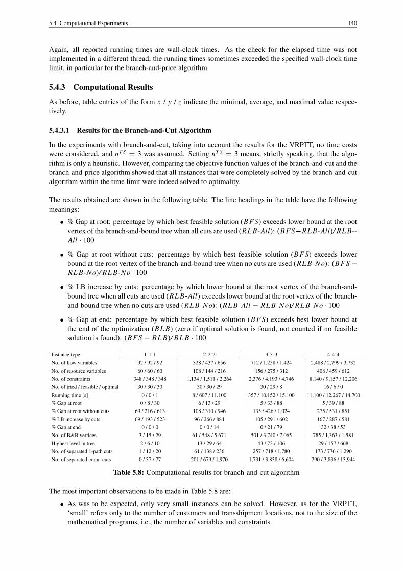
5.4 Computational Experiments 140
Again, all reported running times are wall-clock times. As the check for the elapsed time was notimplemented in a different thread, the running times sometimes exceeded the specified wall-clock timelimit, in particular for the branch-and-price algorithm.
5.4.3 Computational Results
As before, table entries of the form x / y / z indicate the minimal, average, and maximal value respec-tively.
5.4.3.1 Results for the Branch-and-Cut Algorithm
In the experiments with branch-and-cut, taking into account the results for the VRPTT, no time costswere considered, and nT S
= 3 was assumed. Setting nT S= 3 means, strictly speaking, that the algo-
rithm is only a heuristic. However, comparing the objective function values of the branch-and-cut and thebranch-and-price algorithm showed that all instances that were completely solved by the branch-and-cutalgorithm within the time limit were indeed solved to optimality.
The results obtained are shown in the following table. The line headings in the table have the followingmeanings:
• % Gap at root: percentage by which best feasible solution (B F S) exceeds lower bound at the rootvertex of the branch-and-bound tree when all cuts are used (RL B-All): (B F S−RL B-All)/ RL B--All · 100
• % Gap at root without cuts: percentage by which best feasible solution (B F S) exceeds lowerbound at the root vertex of the branch-and-bound tree when no cuts are used (RL B-No): (B F S−RL B-No)/ RL B-No · 100
• % LB increase by cuts: percentage by which lower bound at the root vertex of the branch-and-bound tree when all cuts are used (RL B-All) exceeds lower bound at the root vertex of the branch-and-bound tree when no cuts are used (RL B-No): (RL B-All − RL B-No)/ RL B-No · 100
• % Gap at end: percentage by which best feasible solution (B F S) exceeds best lower bound atthe end of the optimization (BL B) (zero if optimal solution is found, not counted if no feasiblesolution is found): (B F S − BL B)/ BL B · 100
Instance type 1 1 1 2 2 2 3 3 3 4 4 4
No. of flow variables 92 / 92 / 92 328 / 437 / 656 712 / 1,258 / 1,424 2,488 / 2,799 / 3,732No. of resource variables 60 / 60 / 60 108 / 144 / 216 156 / 275 / 312 408 / 459 / 612No. of constraints 348 / 348 / 348 1,134 / 1,511 / 2,264 2,376 / 4,193 / 4,746 8,140 / 9,157 / 12,206No. of tried / feasible / optimal 30 / 30 / 30 30 / 30 / 29 30 / 29 / 8 16 / 6 / 0Running time [s] 0 / 0 / 1 8 / 607 / 11,100 357 / 10,152 / 15,100 11,100 / 12,267 / 14,700% Gap at root 0 / 8 / 30 6 / 13 / 29 5 / 33 / 88 5 / 39 / 88% Gap at root without cuts 69 / 216 / 613 108 / 310 / 946 135 / 426 / 1,024 275 / 531 / 851% LB increase by cuts 69 / 193 / 523 96 / 266 / 884 105 / 291 / 602 167 / 287 / 581% Gap at end 0 / 0 / 0 0 / 0 / 14 0 / 21 / 79 32 / 38 / 53No. of B&B vertices 3 / 15 / 29 61 / 548 / 5,671 501 / 3,740 / 7,065 785 / 1,363 / 1,581Highest level in tree 2 / 6 / 10 13 / 29 / 64 43 / 73 / 106 29 / 157 / 668No. of separated 1-path cuts 1 / 12 / 20 61 / 138 / 236 257 / 718 / 1,780 173 / 776 / 1,290No. of separated conn. cuts 0 / 37 / 77 201 / 679 / 1,970 1,731 / 3,838 / 6,604 290 / 3,836 / 13,944
Table 5.8: Computational results for branch-and-cut algorithm
The most important observations to be made in Table 5.8 are:
• As was to be expected, only very small instances can be solved. However, as for the VRPTT,‘small’ refers only to the number of customers and transshipment locations, not to the size of themathematical programs, i.e., the number of variables and constraints.

5.4 Computational Experiments 141
• Again, the difficulty of the instances within the same instance type varies widely.
• The number of vertices in the branch-and-bound tree and the tree levels reached are both very highon average.
• The use of the static and dynamic cuts increases the lower bound at the root vertex of the branch-and-bound tree by a factor of between 2 and 3 on average. This means that the use of the cuts isthe decisive point which enables the algorithm to solve any instances at all.
• Overall, the results are comparable to those obtained with the branch-and-cut algorithm for theVRPTT.
5.4.3.2 Results for the Branch-and-Price Algorithm
The results obtained for the branch-and-price algorithm with the different pricing problem solution strate-gies are shown in the following tables. Results for the smallest instance types (1 1 1 and 2 2 2) are notreported. The instances of these types were solved in fractions of a second, and only two of them werenot solved at the root vertex of the branch-and-bound tree.
Even when the entries in the line ‘No. of tried / feasible / optimal’ are the same, the different strategiessometimes differ with respect to the number of subproblems, of (E)SPPRCs per subproblem, of generatedvariables, and with respect to the highest level reached in the branch-and-bound tree. Such differences aredue to the fact that the paths are returned to the master problem in a different sequence by the strategies.This leads to different branching decisions and, hence, to different branch-and-bound trees.
Instance Type 3 3 3 4 4 4 5 5 5 6 6 6No. of tried / feasible / optimal 30 / 30 / 30 30 / 30 / 30 30 / 30 / 30 30 / 30 / 30No. solved optimally at root 25 20 20 12Running time [s] 1 / 4 / 75 1 / 33 / 258 3 / 344 / 8,230 10 / 869 / 6,120Pricing time [% Running time] 77 / 85 / 92 78 / 92 / 98 93 / 98 / 100 93 / 99 / 100No. of subproblems 1 / 19.7 / 403 1 / 32.5 / 243 1 / 27.1 / 545 1 / 95.3 / 1,533No. of (E)SPPRCs per subpr. 25 / 63 / 96 24 / 62 / 112 28 / 82 / 160 21 / 69 / 200No. of labels per (E)SPPRC 268 / 508 / 982 561 / 1,469 / 2,333 1,788 / 4,644 / 13,012 3,057 / 9,268 / 23,945No. of generated variables 46 / 184 / 2,222 91 / 524 / 3,287 145 / 869 / 15,414 236 / 1,788 / 17,421Highest level in tree 1 / 3.0 / 27 1 / 5.5 / 24 1 / 3.9 / 31 1 / 7.8 / 34No. of tours 1 / 1.77 / 2 2 / 2.37 / 3 2 / 2.63 / 3 2 / 3.1 / 4No. of LTC Tours 0 / 1.13 / 2 0 / 1.73 / 2 1 / 1.87 / 3 2 / 2.5 / 3Longest Tour [No. of arcs] 4 / 7.4 / 11 5 / 8.27 / 11 6 / 8.87 / 14 6 / 8.97 / 12
Table 5.9: Computational results for unidirectional strategyInstance Type 7 7 7 8 8 8 9 9 9 10 10 10No. of tried / feasible / optimal 30 / 30 / 26 30 / 28 / 16 30 / 20 / 4 30 / 21 / 2No. solved optimally at root 12 8 1 0Running time [s] 22 / 2,659 / 12,300 49 / 5,965 / 14,600 115 / 11,894 / 36,200 1,860 / 15,782 / 45,900Pricing time [% Running time] 97 / 99 / 100 98 / 100 / 100 98 / 100 / 100 100 / 100 / 100No. of subproblems 1 / 94.2 / 1,077 1 / 211.2 / 1,365 1 / 63.6 / 535 1 / 40.2 / 145No. of (E)SPPRCs per subpr. 21 / 65 / 164 14 / 56 / 160 15 / 37 / 116 14 / 44 / 184No. of labels per (E)SPPRC 5,802 / 16,851 / 83,877 7,411 / 25,572 / 81,969 14,469 / 65,572 / 125,673 42,288 / 94,858 / 160,782No. of generated variables 265 / 1,723 / 12,171 306 / 2,718 / 23,879 426 / 1,184 / 3,799 624 / 1,023 / 1,987Highest level in tree 1 / 8.4 / 36 1 / 16.2 / 131 1 / 12.9 / 94 1 / 9.6 / 60No. of tours 3 / 3.8 / 4 3 / 4.14 / 6 4 / 4.35 / 5 4 / 5.38 / 9No. of LTC tours 2 / 3.07 / 4 2 / 3.68 / 5 3 / 3.95 / 4 2 / 4.19 / 6Longest Tour [No. of arcs] 7 / 8.97 / 11 7 / 9.93 / 13 8 / 10.65 / 14 8 / 10.62 / 18
Table 5.10: Computational results for unidirectional strategy (cont.)

5.4 Computational Experiments 142
Instance Type 3 3 3 4 4 4 5 5 5 6 6 6No. of tried / feasible / optimal 30 / 30 / 30 30 / 30 / 30 30 / 30 / 29 30 / 30 / 30No. solved optimally at root 25 20 20 12Running time [s] 1 / 5 / 86 1 / 46 / 358 4 / 516 / 11,100 11 / 1,193 / 6,080Pricing time [% Running time] 79 / 87 / 98 82 / 93 / 99 95 / 98 / 100 94 / 99 / 100No. of subproblems 1 / 19.7 / 403 1 / 33.9 / 279 1 / 16.3 / 233 1 / 92.7 / 1,533No. of (E)SPPRCs per subpr. 25 / 63 / 96 24 / 62 / 112 28 / 82 / 160 21 / 69 / 200No. of labels per (E)SPPRC 304 / 532 / 1,159 608 / 1,332 / 2,100 1,741 / 3,852 / 10,268 2,563 / 6,183 / 12,909No. of generated variables 46 / 184 / 2,229 91 / 546 / 3,843 145 / 525 / 5,223 236 / 1,755 / 17,522Highest level in tree 1 / 2.9 / 27 1 / 5.5 / 24 1 / 3.6 / 22 1 / 7.7 / 31No. of tours 1 / 1.77 / 2 2 / 2.37 / 3 2 / 2.63 / 3 2 / 3.1 / 4No. of LTC tours 0 / 1.13 / 2 0 / 1.73 / 2 1 / 1.87 / 3 2 / 2.53 / 3Longest Tour [No. of arcs] 4 / 7.4 / 11 5 / 8.37 / 12 6 / 8.9 / 14 6 / 9.03 / 12
Table 5.11: Computational results for bidirectional strategy
Instance Type 7 7 7 8 8 8 9 9 9 10 10 10No. of tried / feasible / optimal 30 / 30 / 25 30 / 29 / 15 30 / 23 / 9 30 / 25 / 7No. solved optimally at root 12 8 4 4Running time [s] 27 / 3,420 / 14,900 93 / 6,687 / 16,200 148 / 11,116 / 52,900 2,140 / 11,200 / 15,400Pricing time [% Running time] 99 / 99 / 100 98 / 100 / 100 99 / 100 / 100 100 / 100 / 100No. of subproblems 1 / 83.2 / 775 1 / 139.2 / 1,313 1 / 26.7 / 153 1 / 18.8 / 87No. of (E)SPPRCs per subpr. 21 / 66 / 164 14 / 54 / 160 14 / 54 / 156 12 / 56 / 188No. of labels per (E)SPPRC 5,228 / 9,739 / 41,418 6,431 / 13,953 / 31,110 7,454 / 16,294 / 36,591 11,351 / 36,151 / 291,166No. of generated variables 265 / 1,570 / 9,873 306 / 1,756 / 11,013 426 / 7,566 / 28,342 625 / 4,958 / 16,458Highest level in tree 1 / 8.6 / 43 1 / 13.6 / 78 1 / 7.2 / 59 1 / 4.8 / 13No. of tours 3 / 3.8 / 4 3 / 4.14 / 6 3 / 4.27 / 5 4 / 4.76 / 6No. of LTC tours 2 / 3.13 / 4 2 / 3.66 / 5 3 / 3.86 / 5 3 / 4.48 / 6Longest Tour [No. of arcs] 7 / 9.07 / 12 7 / 10.24 / 13 8 / 10.23 / 13 8 / 10.12 / 14
Table 5.12: Computational results for bidirectional strategy (cont.)
Instance Type 3 3 3 4 4 4 5 5 5 6 6 6No. of tried / feasible / optimal 30 / 30 / 30 30 / 30 / 30 30 / 30 / 28 30 / 30 / 27No. solved optimally at root 25 20 20 12Running time [s] 1 / 11 / 130 1 / 139 / 1,060 8 / 1,149 / 12,900 21 / 2,799 / 14,500Pricing time [% Running time] 83 / 92 / 100 85 / 96 / 100 96 / 99 / 100 97 / 100 / 100No. of subproblems 1 / 19.6 / 403 1 / 33.4 / 261 1 / 12.3 / 89 1 / 90.3 / 1,535No. of (E)SPPRCs per subpr. 31 / 70 / 100 31 / 72 / 128 36 / 93 / 200 31 / 80 / 196No. of labels per (E)SPPRC 365 / 1,200 / 4,604 799 / 2,974 / 7,084 2,929 / 11,595 / 64,898 5,194 / 19,019 / 43,595No. of generated variables 46 / 187 / 2,325 91 / 544 / 3,666 145 / 422 / 1,891 236 / 1,626 / 17,510Highest level in tree 1 / 3.0 / 27 1 / 5.5 / 24 1 / 3.6 / 22 1 / 7.7 / 32No. of tours 1 / 1.77 / 2 2 / 2.37 / 3 2 / 2.67 / 4 2 / 3.1 / 4No. of LTC tours 0 / 1.13 / 2 0 / 1.73 / 2 1 / 1.9 / 3 2 / 2.53 / 3Longest Tour [No. of arcs] 4 / 7.4 / 11 5 / 8.37 / 12 6 / 8.97 / 14 6 / 9.03 / 12
Table 5.13: Computational results for incremental state space augmentation strategy
Instance Type 7 7 7 8 8 8 9 9 9 10 10 10No. of tried / feasible / optimal 30 / 30 / 21 30 / 26 / 14 7 / 4 / 1 0 / 0 / 0No. solved optimally at root 12 8 1 –Running time [s] 48 / 5,156 / 25,200 186 / 7,620 / 24,400 283 / 9,671 / 15,500 –Pricing time [% Running time] 99 / 100 / 100 99 / 100 / 100 100 / 100 / 100 –No. of subproblems 1 / 56.1 / 617 1 / 67.6 / 641 1 / 20.0 / 33 –No. of (E)SPPRCs per subpr. 20 / 75 / 176 23 / 70 / 208 22 / 47 / 128 –No. of labels per (E)SPPRC 8,604 / 31,091 / 127,581 13,118 / 59,687 / 163,704 26,119 / 115,161 / 158,989 –No. of generated variables 265 / 1,039 / 6,396 306 / 1,157 / 9,056 499 / 733 / 1,300 –Highest level in tree 1 / 7.1 / 24 1 / 7.2 / 20 1 / 5.3 / 8 –No. of tours 3 / 3.87 / 4 0 / 3.67 / 6 0 / 2.57 / 5 –No. of LTC tours 2 / 3.1 / 4 0 / 3.07 / 5 0 / 2.29 / 4 –Longest Tour [No. of arcs] 7 / 9.07 / 11 0 / 8.6 / 13 0 / 5.71 / 11 –
Table 5.14: Computational results for incremental state space augmentation strategy (cont.)

5.4 Computational Experiments 143
Instance Type 3 3 3 4 4 4 5 5 5 6 6 6No. of tried / feasible / optimal 30 / 30 / 29 30 / 30 / 30 30 / 30 / 30 30 / 30 / 29No. solved optimally at root 24 20 20 13Running time [s] 1 / 3 / 41 1 / 12 / 99 2 / 31 / 460 7 / 162 / 2,090Pricing time [% Running time] 70 / 80 / 92 63 / 87 / 96 84 / 95 / 100 84 / 96 / 99No. of subproblems 1 / 16.5 / 325 1 / 27.3 / 225 1 / 13.3 / 241 1 / 91.8 / 2,009No. of (E)SPPRCs per subpr. 19 / 56 / 84 19 / 56 / 104 20 / 72 / 136 20 / 62 / 164No. of labels per (E)SPPRC 242 / 421 / 739 510 / 1,097 / 1,867 1,410 / 2,960 / 7,625 1,716 / 4,703 / 9,821No. of generated variables 46 / 170 / 1,977 91 / 438 / 2,991 145 / 514 / 6,770 232 / 1,601 / 24,809Highest level in tree 1 / 2.9 / 29 1 / 4.9 / 24 1 / 2.8 / 21 1 / 6.9 / 34No. of tours 1 / 1.77 / 2 2 / 2.37 / 3 2 / 2.63 / 3 2 / 3.1 / 4No. of LTC tours 0 / 1.13 / 2 0 / 1.73 / 2 1 / 1.87 / 3 2 / 2.53 / 3Longest Tour [No. of arcs] 4 / 7.3 / 11 5 / 8.27 / 11 6 / 8.9 / 14 6 / 8.97 / 12
Table 5.15: Computational results for heuristic algorithm
Instance Type 7 7 7 8 8 8 9 9 9 10 10 10No. of tried / feasible / optimal 30 / 30 / 25 30 / 30 / 15 30 / 30 / 4 30 / 30 / 2No. solved optimally at root 12 7 1 1Running time [s] 15 / 1,000 / 8,540 33 / 4,400 / 14,500 68 / 5,939 / 14,400 128 / 11,818 / 111,000Pricing time [% Running time] 91 / 97 / 100 92 / 97 / 100 93 / 98 / 100 94 / 99 / 100No. of subproblems 1 / 122.9 / 1,403 1 / 882.6 / 6,015 1 / 446.1 / 2,359 1 / 361.3 / 1,549No. of (E)SPPRCs per subpr. 21 / 60 / 160 12 / 51 / 156 12 / 46 / 156 10 / 50 / 188No. of labels per (E)SPPRC 3,591 / 8,387 / 48,737 4,118 / 10,180 / 45,200 7,454 / 16,107 / 36,591 11,351 / 48,625 / 461,214No. of generated variables 265 / 2,712 / 28,870 306 / 9,555 / 32,111 426 / 8,775 / 28,342 625 / 5,340 / 16,458Highest level in tree 1 / 8.3 / 31 1 / 16.7 / 80 1 / 25.8 / 202 1 / 20.6 / 107No. of tours 3 / 3.8 / 4 3 / 4.03 / 5 3 / 4.2 / 5 4 / 4.73 / 6No. of LTC tours 2 / 3.13 / 4 3 / 3.67 / 5 3 / 3.87 / 5 3 / 4.47 / 6Longest Tour [No. of arcs] 7 / 8.93 / 11 7 / 9.9 / 13 8 / 10.37 / 13 8 / 10.23 / 14
Table 5.16: Computational results for heuristic algorithm (cont.)
Pricing problem strategy Unidirectional Bidirectional ISSA HeuristicNo. of tried / feasible / optimal 240 / 219 / 168 240 / 229 / 175 187 / 180 / 151 240 / 240 / 164No. solved optimally at root 98 105 98 98Running time [s] 1 / 3,898 / 45,900 1 / 3,899 / 52,900 1 / 2,858 / 25,200 1 / 2,921 / 111,000Pricing time [% Running time] 77 / 96 / 100 79 / 97 / 100 83 / 98 / 100 63 / 94 / 100No. of subproblems 1 / 73.5 / 1,533 1 / 55.1 / 1,533 1 / 45.5 / 1,535 1 / 245.2 / 6,015No. of (E)SPPRCs per subpr. 14 / 61 / 200 12 / 64 / 200 20 / 75 / 208 10 / 57 / 188No. of labels per (E)SPPRC 268 / 22,839 / 160,782 304 / 10,248 / 291,166 365 / 24,455 / 163,704 242 / 11,560 / 461,214No. of generated variables 46 / 1,251 / 23,879 46 / 2,118 / 28,342 46 / 825 / 17,510 46 / 3,638 / 32,111Highest level in tree 1 / 8.1 / 131 1 / 6.7 / 78 1 / 5.6 / 32 1 / 11.1 / 202
Table 5.17: Comparison of computational results for branch-and-price algorithm
The most important observations to be made in Tables 5.9–5.17 are:
• The difficulty of the instances varies widely. For example, the shortest running time for the unidi-rectional strategy for a 7 7 7 instance is 22 seconds, the longest is 12,300 seconds (which is morethan 500 times longer).
• About 40 % of the instances were solved optimally without branching.
• The pricing step is by far the most time-consuming part in all strategies.
• The number of (E)SPPRCs per subproblem, i.e., the number of column generation iterations, israther high. The numbers indicated in the lines ‘No. of labels per (E)SPPRC’ must be divided byfour, because at each iteration, there are four different (E)SPPRCs that have to be solved, one foreach vehicle (class). Still, the average number of (E)SPPRCs per subproblem ranges between 15and 19.

5.5 Conclusions 144
• The unidirectional strategy is the best exact strategy for the instance types up to 7 7 7. It is thefastest and computes optimal solutions to more instances than the other two exact strategies.
• The bidirectional strategy is superior for the large instance types. It is faster, computes feasiblesolutions to more instances, and solves more instances to optimality than the other two exactstrategies. With the exception of the 3 3 3 instances, it always creates fewer labels than the othertwo exact strategies; for the 10 10 10 instances, it even creates fewer labels than the heuristicstrategy. Profiling of the code has shown that the reason why the bidirectional strategy is slowerfor the small instances is the time-consuming join operation. (Without the additional join testdescribed on page 132, the join operation would have taken much longer still.) For the largeinstances, this effect is overcompensated by the lower number of created labels. These results arein accordance with the findings of Salani 2005.
• The incremental state space augmentation strategy is clearly the worst strategy. The number of(E)SPPRCs that are solved per subproblem and the number of created labels are much higher thanwith the other strategies. These results are contrary to the findings of Salani 2005 and Boland et al.2006. A possible explanation is that the absence of time windows in the test instances leads toexcessive cycling.
• The performance of the heuristic strategy is very good. Feasible solutions are computed for allinstances, and the largest gap between the heuristic and the optimal solution is less than 0.25 %.A pairwise comparison of running times shows that the heuristic strategy is about 1.8 times as fastas the unidirectional strategy and twice as fast as the bidirectional strategy, but more than 95 % ofthe instances are solved to optimality. Due to the time limits, there are no fewer than 50 instanceswhere the heuristic obtained a better solution than the unidirectional strategy.
5.5 Conclusions
The chapter has presented an arc-variable-based and a path-variable-based formulation for the TTRPincluding some extensions not yet covered in the literature, most notably, optional parking and trans-shipment locations. Moreover, the chapter has described the first two exact solution procedures for theproblem, a branch-and-cut and a branch-and-price algorithm.
The decisive advantages of the branch-and-price algorithm over the branch-and-cut algorithm are:
• The pricing problems can be solved exactly on a smaller network than the one on which the arcvariable formulation is based.
• Fleet planning (deciding on the number of vehicles of each available type that should be used) andvehicle routing can be performed simultaneously without additional modelling or computationaleffort.
Extensive computational experiments with implementations of both algorithms have been performed.The tests have been executed on randomly generated instances structured to resemble real-world sit-uations. The experiments have shown that the branch-and-price algorithm is clearly superior to thebranch-and-cut algorithm. The former is able to solve instances which are one order of magnitude largerthan those solvable by the latter. However, even with a heuristic algorithm based on branch-and-price,only instances considerably smaller than typical real-world instances can be solved.
The largest instances that could be solved to optimality comprised 20 customers, 20 transshipment lo-cations, four types of vehicle, and no time windows. The following quote from Fukasawa et al. 2006,p. 492, on the VRPTW with homogeneous fleet, puts these computational results into perspective: ‘Itshould be noted that . . . column generation has been the dominant approach for the Vehicle Routing Prob-lem with Time Windows (VRPTW). Current branch-and-price algorithms can consistently solve tightly
5.5 Conclusions 145
constrained instances (those with narrow time windows) with up to 100 clients. However, they often failon less constrained instances with only 50 clients.’ This shows that the developed implementation is ona par with existing branch-and-price codes.
This chapter has provided an answer to the question posed in Section 4.3.2.6, ‘which aspects of theVRPTT can be considered in a model that can still be solved exactly?’: When comparing the arc variableformulations of the VRPTT and the TTRP, the reader cannot fail to notice that the VRPTT formula-tion is more elegant and easier to understand. However, comparing the path variable formulations ofthe problems and the growth rates of the underlying networks with increasing number of customers,transshipment locations, and vehicles, it becomes evident that the step from a fixed to a free lorry-trailerassignment constitutes the decisive leap in complexity. The synchronization constraints for lorries andtrailers are apparently a point where matters become really difficult. Conversely, the TTRP is on a levelof complexity that may still be considered tractable by exact algorithms.

Chapter 6
Possible Lines of Research
None of the three considered generalized routing problems could be treated exhaustively; much remainsto be investigated. This chapter describes interesting lines of research that could not be pursued in thetime available for this paper.
6.1 The GDRPP
6.1.1 Alternative Formulations
In the computational experiments for the GDRPP, only formulation (3.6) was solved by branch-and-cut.The other two formulations, (3.3) and (3.5), could be tested as well.
6.1.2 Improvements of Branch-and-Cut
The branch-and-cut algorithm for formulation (3.6) still leaves much room for improvement. Most im-portantly, a thorough polyhedral investigation should be made to identify further valid inequalities, andfor the GDRPP (contrary to the VRPTT and the TTRP), it is still promising to try to prove which ofthem induce facets. Additional valid inequalities could be derived (generalized), for example, from theknown cuts for the GATSP, the WRPP (taking into account that an arc is a special kind of windy link), orthe so-called road travelling salesman problem (RTSP) (Fleischmann 1985). Recent theoretical paperson the WRPP and the windy general routing problem (WGRP) are Corberan et al. 2003, Corberan et al.2004, Corberan et al. 2005a, Corberan et al. 2005b. The branch-and-cut algorithm could also benefitfrom a tailored branching strategy (e.g., branch on the δi variables first).
6.1.3 Further Possibilities
There is not much literature on the DRPP (Campos/Savall 1995 present a cutting plane algorithm), sothat it would be worthwhile to make experiments with formulation (3.1), too.
In addition, the two direct formulations for the WRPPTP should be compared theoretically and empiri-cally. Moreover, of the three possibilities to transform a graph with turn penalties into one without, onlytwo were used in the computational experiments. The ‘dual graph’ approach should also be tried.
For instances with many zigzag links, it would be worthwhile to try to exploit the special structure of theresulting two non-disjoint r-groups in a solution algorithm.
The computational results showed that the solution quality of the heuristics is not very good. Additionallocal search improvement procedures and/or the use of metaheuristics should be considered. This couldbe helpful for the branch-and-cut algorithm, too.
146

6.2 The VRPTT 147
When solving the GDRPP exactly or heuristically by a labelling algorithm, it is easily possible to con-sider resource constraints, most notably time windows. ARPs with time windows are rarely addressedin the literature (see, for example, Dror/Langevin 2000), despite the fact that time windows are just asrelevant in arc routing applications as they are relevant in TSP or VRP applications. The exact labellingalgorithm should be able to solve much larger instances when tight time windows are given.
As shown above, it is easy to transform the GDRPP into the GATSP. This means that all consideredproblems can also be solved as GATSPs. It would be interesting to examine for which problem whichtransformation (into GDRPP or into GATSP) is more easily solved by branch-and-cut and to comparethe branch-and-cut algorithm for the GDRPP to existing exact GATSP procedures.
6.2 The VRPTT
6.2.1 Alternative Formulations
The turn variable formulation should also be restricted to the core problem, solved by branch-and-cut,and compared to the arc variable formulation. In addition, the discretized formulations should be im-plemented and tested empirically. In particular, experiments should be made with different load transferamounts (cf. Del Pia/Filippi 2006).
Two difficulties with the MIP formulations for the VRPTT presented in Chapter 4 are that the networkson which the formulations are based quickly become intractably large with increasing instance size andthat the formulations contain a lot of logical constraints that must be linearized by using large constantsM . (This is the main reason why the LP relaxation of (4.59)–(4.62) is so weak.) The branch-and-priceapproach offers only a partial remedy: Several implications are pricing problem constraints in the pathvariable formulation. When the pricing problems are solved by a labelling algorithm, these implicationsare represented in the REFs, and the Ms are essentially removed. However, there are still many impli-cations in the master problem. A technique that takes a different approach to problem representation ingeneral and in particular to logical constraints is constraint programming (Lustig/Puget 2001, Hooker2002, Van Hentenryck 2002). Constraint programming is able to directly represent and solve logicalimplications without having to take the indirection of M constants, and it may also offer ways of rep-resenting the load transfer logic more efficiently. So, constraint programming is an alternative for the(exact as well as heuristic) solution of the VRPTT that should be seriously explored.
In recent years, there have been efforts to integrate mixed integer programming and constraint program-ming in order to combine the strengths of both methods. A paper that demonstrates the viability of theconstraint programming approach for the solution of problems with many logical constraints is Codato/Fischetti 2006. The authors use so-called combinatorial Benders’ cuts to get rid of the M constantsin MIP formulations. They report very promising computational results for problems known from theliterature and show that their approach clearly outperforms CPLEX for such problems.
6.2.2 Improvements of Branch-and-Cut
The lower bounds in the branch-and-cut algorithm are still very weak and should be improved. Sev-eral possibilities exist for finding additional cuts. Many different classes of valid inequalities for thesymmetric VRP without time windows are known (cf. Lysgaard et al. 2004, Fukasawa et al. 2006). Inprinciple, such inequalities should also be applicable to the VRPTT (Grunert/Irnich 2005b, p. 427).For the asymmetric VRPTW, Kallehauge et al. 2005, p. 85 ff., describe different valid inequalities andmention references where these inequalities were used in branch-and-cut or branch-and-price-and-cutalgorithms. It would be very interesting to investigate further how all these inequalities, in particular,the κ-path cuts, can effectively and efficiently be generalized for the VRPTT, or, at least, for VRPs withheterogeneous fleet.

6.2 The VRPTT 148
Upper bounds are useful, too. Such bounds could be computed by solving the corresponding TTRP ex-actly or heuristically, or by a heuristic for the VRPTT.
The number of variables and constraints in the arc variable formulation, although polynomial in thenumber of customers, transshipment locations, and vehicles, increases sharply with increasing numberof these objects. Therefore, it would be worthwhile to try to use the concept of lazy constraints to speedup the solution process. Contrary to the ‘real’ cuts described in Section 4.5.1 (inequalities such as thesupply collection and the lorry flow cut), lazy constraints are irredundant but unlikely to be violated by anoptimal solution to the LP relaxation of the formulation without them. Hence, they may be omitted whenthe LP relaxation is solved, and they must be checked for violation only afterwards. All violated lazyconstraints must then be added to the LP relaxation, and the latter must be re-solved. This procedure mustbe repeated until no more lazy constraints are violated, in which case the solution to this ‘restricted’ LPrelaxation is an optimal solution to the ‘complete’ LP relaxation. Constraints such as (4.60e) and (4.60h)–(4.60j) account for a considerable number of all constraints in the VRPTT arc variable formulation. Suchconstraints are promising lazy constraint candidates, as their omission might significantly speed up thesolution of the LP relaxation.
6.2.3 Improvements of Branch-and-Price
The first and decisive ‘improvement’ on the branch-and-price approach would be to actually implementit. At first, the pricing problems could be solved by branch-and-cut. To keep the subproblem networksas small as possible, the problems should at first be solved with nT S
= 2 or nT S= 3 until no more
negative reduced cost paths are found. Then, nT S could be increased in the respective subnetworks forthose transshipment locations which are actually used. If the results are promising, tackling the pricingproblems by a labelling algorithm could be tried.
Generally, solving ESPPRCs by branch-and-cut is an interesting approach in itself. There are practicallyno publications in this field. Starting with the ESPPTW with negative cycles, valid inequalities for ESP-PRCs should be investigated.
The (E)SPPRC is similar to a multi-criteria optimization problem. Research in this field is becomingmore and more intense (cf. the survey Ehrgott/Gandibleux 2000). A thorough survey of the pertinentliterature might lead to new insights for solving negative-cycle (E)SPPRCs.
6.2.4 Further Possibilities
Taking into account the results of the computational experiments in Chapter 4 and the practical relevanceof the problem, what is most urgently needed is a good heuristic capable of solving realistic instanceswith hundreds of customers and dozens of transshipment locations.
In airline crew scheduling problems, the issue of robustness of solutions to modifications of the datais becoming increasingly important (cf. Lan et al. 2006). It is desirable to compute solutions that arerelatively insensitive to unexpected events happening in practice (delays etc.). The flight plans should besuch that as few other flights, respectively, passengers, as possible are affected when one flight is late.The solutions to VRPTTs are also susceptible to such effects. When trailers or support vehicles arrivelate at transshipment locations, other vehicles are affected, and infeasibilities due to time window viola-tions may occur. Hence, solutions to VRPTTs should be evaluated in this respect, and ideally, (heuristic)algorithms for solving practical problems should be constructed so as to favour ‘robust’ solutions. (In theTTRP, robustness of solutions (with respect to time) is not an issue. Different vehicles do not influenceone another.)
The idea of discretizing the load transfer amounts maintains exactness of the formulation in cases wherethe goods to be collected at (or delivered to) customers are not homogeneous. For example, there are

6.3 The TTRP 149
many applications where the goods consist in swap-body platforms or containers. The lorries and trailersused for such transports each have capacity one, i.e., they are able to transport one container at a time,which makes load synchronization between lorry and trailer trivial. Such problems constitute a verypromising application area for VRPTT models and algorithms.
Another application area for VRPTT models or, at least, for models considering support vehicles, is bi-modal traffic road/rail. Trains cannot usually visit customers and can therefore be modelled as supportvehicles. Trains normally have fixed schedules, so at least the temporal synchronization between collec-tion vehicles (lorries and trailers) and support vehicles (trains) is easy.
A potential extension of the VRPTT is the pickup-and-delivery problem with trailers and transshipments(PDPTT). This is particularly interesting for networks of less-than-truckload forwarders, where it is com-mon to use transshipment locations to transfer consignments between feeder, long-haul, and distributionvehicles.
It is possible to consider more complex synchronization requirements. For example, when drivers arealso considered, a trailer needs two other objects to be able to move in space, a lorry and a driver, so thatthree types of object have to be synchronized. An even more complex situation is the transport of con-signments which must be transported in swap-body platforms. These platforms may only be transportedby trailers, which in turn must be pulled by lorries, which must be operated by drivers. In this case, fivedifferent types of object must be synchronized.
The concept of a turn in a graph was originally used in arc routing applications modelling turn restric-tions and prohibitions in real road networks. As shown in Chapter 4, turn variables can also be sensible ifthere are no such restrictions. It would be very interesting to evaluate the benefits of formulations usingturn variables for other types of routing problem.
The above formulations for the VRPTT consider the underlying real-world problem from a routing per-spective. It may also be interesting to view the problem from a scheduling perspective, where there arejobs to be performed (customers to be served) and the assignment of these jobs to machines (lorries) andthe sequence in which each machine performs its assigned jobs are to be determined. To perform a job,a machine needs resources (loading capacity). If a machine does not have enough resources to performa job, it must use auxiliary resources (trailers).
The VRPTT is a concrete case of an abstract ‘time-constrained vehicle routing and scheduling prob-lem with multiple synchronization (or multiple logically coupling) constraints’. These synchronizationconstraints contain resource variables, thus making a branch-and-price approach difficult. It would beinteresting to study this class of problem on a more abstract level and to examine more closely how it fitsinto the unified model of Desaulniers et al. 1998.
6.3 The TTRP
6.3.1 Alternative Formulations
In the arc variable formulation, it would be possible to use xki j variables that may take the three values
0, 1, and 2, where xki j = 2 means that LTC lorry k traverses arc (i, j) with its trailer attached. This
would make the yki j variables obsolete. However, it is not immediately clear whether this would have
been a better approach (for example, the consideration of the trailer costs in the objective function is notso straightforward then).
As explained above, the formulation given by Scheuerer 2004 does not use logical implications andtherefore does not need any M constants. It would be interesting to implement this formulation and toperform computational experiments to see how it compares with the arc variable formulation presentedhere.
6.3 The TTRP 150
The networks for TTRPs do not grow as fast as those for the VRPTT. Moreover, all logical constraints inthe TTRP are pricing problem constraints and are represented in the REFs, so that no M issue arises inthe branch-and-price approach. Therefore, a constraint programming approach is not so interesting here,but if such an approach proves successful for the VRPTT, it could also be tried for the TTRP.
6.3.2 Improvements of Branch-and-Cut
The comments in the corresponding section on the VRPTT apply here analogously. Additionally, itmust be mentioned that, contrary to CPLEX, the ABACUS framework does not include general cuts likeGomory cuts or flow cover cuts. Such cuts were automatically added by CPLEX in the computationalexperiments for the VRPTT, and they would have increased the solution speed of the branch-and-cutalgorithm for the TTRP, too.
6.3.3 Improvements of Branch-and-Price
The implementation of the branch-and-price algorithm presented in the previous chapter is more than abare proof of concept. However, given the current state of research on column generation and branch-and-price, it is simply impossible for an individual to include all currently known acceleration techniquesand refinements in a code within a reasonable amount of time. Therefore, the implementation can stillbe improved significantly. The most important refinements are:
• The inclusion of stabilization in the column generation process (Lubbecke/Desrosiers 2005, p.1017 ff.).One problem with column generation algorithms in general is the so-called tailing-off effect, whichmeans a slow convergence at the end of the process. This can be due to several reasons; theeffect, however, is not yet completely understood theoretically. Nevertheless, there are severalpossibilities for speeding up the procedure. The simplest method is to add more than one columnto the master problem at a time. This has been done in the algorithm of Chapter 5. Another optionis to use interior point methods for the solution of the master problem. This has been tried for theTTRP algorithm, but with little effect. More sophisticated techniques are described in Lubbecke/Desrosiers 2005 (ib.). The theory as well as the implementation of such techniques is non-trivial.The number of (E)SPPRCs solved at each vertex of the branch-and-price tree is an indicator forthe potential usefulness of stabilization. As the computational experiments showed, this numberwas rather high, so that a powerful stabilization algorithm should be the first improvement madein the TTRP branch-and-price algorithm.
• The use of a primal heuristic to quickly obtain good upper bounds.The procedures by Chao 2002 and Scheuerer 2004 could be used for this purpose.
• The development of better lower bounding procedures.Any progress in the research on valid inequalities for the VRPTT and the TTRP could possiblyalso be put to good use in the TTRP branch-and-price algorithm, which might then be augmentedto become a branch-and-price-and-cut procedure.
A possible improvement on the dominance check in the labelling algorithm for the solution of the pricingproblems is multidimensional divide-and-conquer (cf. Kung et al. 1975, Bentley 1980). This algorithm,respectively, algorithmic paradigm, is particularly hard to implement if there are non-integer resources,as is the case in branch-and-price algorithms because of the dual prices. On 64-bit computers and withcompilers with 64-bit integer types, it would be interesting to transform the dual prices from doubleto int, so that a numerically stable implementation is possible. The complexity of multidimensionaldivide-and-conquer increases logarithmically with the number of resources, so if there are visitationcounters, it is not clear whether the procedure will lead to performance improvements.

6.4 Location-Routing Problems 151
Besides, the solution of the pricing problems may still be accelerated by using further techniques forheuristic pricing. It may also be interesting to test the heuristic approach with the bounded bidirectionaldynamic programming algorithm instead of the unidirectional version. Moreover, the pricing problemscould be solved by branch-and-cut just to see how this approach compares with the labelling algorithmand to see whether it is sensible to try to solve the VRPTT pricing problems by branch-and-cut.
6.3.4 Further Possibilities
For both free and fixed lorry-trailer assignments, i.e., for both the VRPTT (or rather, the VRP withtrailers and without transshipments, VRPTT or VRPT) and the TTRP, it would also be interesting toconsider the case where transshipments are impossible or forbidden. It may be technically impossiblebecause the technical equipment for loading and unloading a good may not be available outside plantsand warehouses. The customer may forbid it, because the goods to be transported may be very fragile.The law may forbid it (e.g., customs-sealed vehicles in international traffic, livestock haulage, transportof hazardous materials). Without transshipments, support vehicles are not useful, but trailers still may be.
Several possibilities for the collection of the supplies are possible. It could be required that the supply ofa trailer customer be entirely loaded onto a trailer, or that it be entirely loaded on either lorry or trailer, orit could still be allowed to split it arbitrarily between lorry and trailer. In any case, capacity constraintsfor the lorries as well as for the trailers are necessary. Depending on the requirements for the collectionof trailer customer supplies, also constraints restricting the total vehicle load may be needed.
When trailer customer supplies must be entirely loaded onto trailers, in both the VRPT and the TTRP,there are no more load synchronization constraints. However, in the VRPT, the constraints for temporalsynchronization at parking locations/vertices and for routing synchronization remain relevant.
6.4 Location-Routing Problems
As already mentioned in Chapter 4, location-routing problems (LRPs, cf. Engele 1980, Laporte 1988,Daskin 1995, p. 339 ff., Nagy/Salhi 1996, Albareda-Sambola et al. 2005) combine facility location withvehicle routing. LRPs simultaneously address the following five questions (Daskin 1995, p. 339 f.):
(i) How many facilities (depots, warehouses, factories) should be located (opened, built, rented)?
(ii) Where should these facilities be located?
(iii) Which customers (regional warehouses, retailers) should be assigned to which facility?
(iv) Which customers should be visited on one and the same vehicle route starting and ending at acertain facility?
(v) In what sequence should the customers on one route be visited?
LRPs come in several variants. Deterministic, single period LRPs can be categorized by the followingfour criteria (cf. Albareda-Sambola et al. 2005, p. 408):
(i) the type of the facilities to be located (are they allowed to be origins and destinations of vehicleroutes or are they only intermediate depots?),
(ii) whether the facilities are capacitated or not,
(iii) whether facilities and/or customers have time windows or not, and
(iv) whether the vehicles are capacitated (or, more generally, homogeneous) or not.

6.4 Location-Routing Problems 152
There are also dynamic and stochastic types of LRP (cf. ib.).
In Chapters 4 and 5, network representations for the VRPTT and the TTRP were presented. Interest-ingly, a similar network was used in Laporte et al. 1988 for the solution of a location-routing problemwith capacitated facilities, no time windows, and capacitated vehicles, where the facilities are allowed tobe origins and destinations of vehicle routes. (The facility capacities are given indirectly by specifyingthe maximal number of vehicle tours that may start and end at a facility.)
All of the sixteen types of LRP that can be distinguished by the above four criteria can be modelled asVRPTTs or TTRPs, and there are several options how to do this.
The main idea is to consider the trailers as abstract, virtual objects for which there are no correspondingobjects in the real world. Trailers are used as modelling tools that serve as the connection between thevehicle(s) (the lorry/lorries) and the potential facilities (the transshipment locations). The visited trans-shipment locations correspond to the facilities to be opened. All customers are lorry customers.
The four criteria of the above taxonomy can be considered as follows in a VRPTT or a TTRP:
(i) One central depot is created where all single lorries and all LTCs start and end their tours. Inthe case where the facilities to be located are allowed to be origins and destinations of vehicleroutes, this depot is a virtual location with a distance of zero to and from any other location. Thefixed costs of opening a facility are added to the trailer costs on arcs entering the correspondingdecoupling vertex. The costs of returning to the virtual depot are set to zero. Moreover, when thelorries must be empty when they return to the central depot, i.e., when the complete supply of thecustomers must be transferred into a trailer at a transshipment location, the load transfer variablesof the lorries are fixed accordingly.
(ii) The (finite or infinite) capacities of the potential facilities are represented by the capacities of thetrailer(s). When the capacities of the potential facilities are finite, there is one LTC for each trans-shipment location (and, hence, for each potential facility), and the capacity of the LTC trailer isequal to the capacity of the corresponding potential facility. If all potential facilities have unlim-ited capacity (and if there are no time windows), there is only one lorry-trailer combination witha trailer with unlimited capacity. Symmetries concerning the sequence of the visited transship-ment locations can then be avoided by assigning artificial pairwise disjoint time windows to thetransshipment locations, thus fixing the sequence in which they may be visited.
(iii) Time windows for potential facilities as well as for customers carry over naturally to the trans-shipment locations and customers. However, if there are time windows, there must be a sufficientnumber of single lorries which may transfer load to the trailers corresponding to the potential facil-ities. Hence, to consider time windows, a VRPTT model must be used. Accessibility constraintsmust then make sure that each single lorry is used only at one facility/transshipment location. Tomodel the case where the potential facilities have time windows and are the origins and destina-tions of vehicle routes, the costs of a single lorry on an arc from the virtual depot to a customerin the VRPTT network is set to the costs of this lorry from its assigned potential facility to therespective customer.
(iv) Capacities for the vehicles in the LRP are represented by the lorry capacities in the VRPTT orTTRP. Again, accessibility constraints are used to ensure that a certain vehicle is used only at thedesired facility.
The above description also applies to the VRPTT when the LTC is replaced by a support vehicle or evenby a single trailer/when the LTCs are replaced by support vehicles or even by single trailers without fixedlorry-trailer assignment.

6.4 Location-Routing Problems 153
The presented transformations of LRPs constitute a promising application area for TTRPs and VRPTTs.If only one LTC is necessary, the LRP can be solved with a labelling algorithm. The difficulty with thesolution of the resulting TTRPs or VRPTTs by branch-and-cut is that nT S then determines the maximalnumber of tours/vehicles for each potential facility in the LRP. When the capacities of the potentialfacilities are finite, and when solving the resulting TTRPs or VRPTTs by branch-and-price, there is onesubproblem per potential facility. For instances where the number of potential facilities is similar to thenumber of customers, an undesirably large number of subproblems must be solved. Therefore, judging bythe results of the computational experiments, LRPs with uncapacitated potential facilities, uncapacitated,homogeneous vehicles, and no time windows should be well solvable as TTRPs or VRPTTs.

Final Remark
On his first day as a university student, the author attended an introductory lecture given by the thenDean of the Economics Faculty at the University of Augsburg. The Dean told his audience that a goodstudent is not only one who has learned to answer a lot of questions, but also one who has learned to aska lot of (interesting) questions.
It is the author’s conviction that both the problems treated in this paper, and the treatment itself, haveleft open and thrown up more questions than could possibly be answered here, and it is his hope that thispaper will be helpful in sparking off interest among its readers to concern themselves further with turns,trailers, and transshipments.
Acknowledgements
Thanks are due to Jacques Desrosiers for helpful hints on the discretized VRPTT, to Christine Stibbe andJens Wollenweber for proofreading the manuscript, to all people at the Deutsche Post Endowed Chair ofOptimization of Distribution Networks for being colleagues in the best sense of the word and providingthe best possible working atmosphere, and in particular to Stefan Irnich for many lively discussions andinvaluable advice.
154

Bibliography
Aho, A.; Hopcroft, J.; Ullman, J. (1983):Data Structures and AlgorithmsAddison-Wesley, Reading
Ahuja, R.; Magnanti, T.; Orlin, J. (1993):Network FlowsPrentice-Hall, Upper Saddle River
Albareda-Sambola, M.; Dıaz, J.; Fernandez, E. (2005):A Compact Model and Tight Bounds for a Combined Location-Routing ProblemComputers & Operations Research, vol. 32, pp. 407–428
Anez, J.; de la Barra, T.; Perez, B. (1996):Dual Graph Representation of Transport NetworksTransportation Research Part B, vol. 30, pp. 209–216
Arkin, E.; Bender, M.; Demaine, E.; Fekete, S.; Mitchell, J.; Sethia, S. (2005):Optimal Covering Tours with Turn CostsSIAM Journal on Computing, vol. 35, pp. 531–566
Assad, A.; Golden, B. (1995):Arc Routing Methods and Applicationsin:Ball, M.; Magnanti, T.; Monma, C.; Nemhauser, G. (eds.):Network RoutingHandbooks in Operations Research and Management Science, vol. 8Elsevier, Amsterdampp. 375–483
Bamberg, G.; Baur, F. (1989):StatistikOldenbourg, Munchen
Barnhart, C.; Johnson, E.; Nemhauser, G.; Savelsbergh, M.; Vance, P. (1998):Branch-and-Price: Column Generation for Solving Huge Integer ProgramsOperations Research, vol. 46, pp. 316–329
Beasley, J.; Christofides, N. (1989):An Algorithm for the Resource Constrained Shortest Path ProblemNetworks, vol. 19, pp. 379–394
Benavent, E.; Corberan, A.; Sanchis, J. (2000):Linear Programming Based Methods for Solving Arc Routing Problemsin:Dror, M. (ed.):Arc Routing: Theory, Solutions, and Applications
155

Bibliography 156
Kluwer, Bostonpp. 231–275
Benavent, E.; Soler, D. (1999):The Directed Rural Postman Problem with Turn PenaltiesTransportation Science, vol. 33, pp. 408–418
Bentley, J. (1980):Multidimensional Divide-and-ConquerCommunications of the ACM, vol. 23, pp. 214–229
Blais, M.; Laporte, G. (2003):Exact Solution of the Generalized Routing Problem Through Graph TransformationsJournal of the Operational Research Society, vol. 54, pp. 906–910
Bodin, L.; Kursh, S. (1978):A Computer-Assisted System for the Routing and Scheduling of Street SweepersOperations Research, vol. 26, pp. 525–537
Bodin, L.; Kursh, S. (1979):A Detailed Description of a Computer System for the Routing and Scheduling of Street SweepersComputers & Operations Research, vol. 6, pp. 181–198
Bodin, L.; Levy, L. (2000):Scheduling of Local Delivery Carrier Routes for the United States Postal Servicein:Dror, M. (ed.):Arc Routing: Theory, Solutions, and ApplicationsKluwer, Bostonpp. 419–442
Boland, N.; Dethridge, J.; Dumitrescu, I. (2006):Accelerated Label Setting Algorithms for the Elementary Resource Constrained Shortest Path ProblemOperations Research Letters, vol. 34, pp. 58–68
Bousonville, T.; Kopfer, H. (2000):A Hybrid Evolutionary Algorithm for the Mixed Rural Postman Problem with Turn PenaltiesTechnical Report, Bremer Institut fur Betriebstechnik und angewandte Arbeitswissenschaft, UniversitatBremen
Bramel, J.; Simchi-Levi, D. (1997):The Logic of LogisticsSpringer, New York
Bramel, J.; Simchi-Levi, D. (2002):Set-Covering-Based Algorithms for the Capacitated VRPin:Toth, P.; Vigo, D. (eds.):The Vehicle Routing ProblemSIAM Monographs on Discrete Mathematics and Applications, Philadelphiapp. 85–108
Brunswicker, J. (1986):Optimale Standort- und Tourenplanung fur die Rohmilcherfassung eines MolkereibetriebesLit, Munster

Bibliography 157
Cabral, E.; Gendreau, M.; Ghiani, G.; Laporte, G. (2004):Solving the Hierarchical Chinese Postman Problem as a Rural Postman ProblemEuropean Journal of Operational Research, vol. 155, pp. 44–50
Caldwell, T. (1961):On Finding Minimum Routes in a Network with Turn PenaltiesCommunications of the ACM, vol. 4, pp. 107–108
Campos, V.; Savall, J. (1995):A Computational Study of Several Heuristics for the DRPPComputational Optimization and Applications, vol. 4, pp. 67–77
Chabrier, A. (2006):Vehicle Routing Problem with Elementary Shortest Path Based Column GenerationComputers & Operations Research, vol. 33, pp. 2972–2990
Chao, I. (2002):A Tabu Search Method for the Truck and Trailer Routing ProblemComputers & Operations Research, vol. 29, pp. 33–51
Chisman, J. (1975):The Clustered Traveling Salesman ProblemComputers & Operations Research, vol. 2, pp. 115–119
Chvatal, V. (1983):Linear ProgrammingFreeman, New York
Clossey, J.; Laporte, G.; Soriano, P. (2001):Solving Arc Routing Problems with Turn PenaltiesJournal of the Operational Research Society, vol. 52, pp. 433–439
Codato, G.; Fischetti, M. (2006):Combinatorial Benders’ Cuts for Mixed-Integer Linear ProgrammingOperations Research, vol. 54, pp. 756–766
Corberan, A.; Martı, R.; Martınez, E.; Soler, D. (2002):The Rural Postman Problem on Mixed Graphs with Turn PenaltiesComputers & Operations Research, vol. 29, pp. 887–903
Corberan, A.; Plana, I.; Sanchis, J. (2004):Zigzag Inequalities: A New Class of Facet-Inducing Inequalities for Arc Routing ProblemsTechnical Report TR04-2004, Departamento de Estadıstica e Investigacion Operativa, Universidad deValencia
Corberan, A.; Plana, I.; Sanchis, J. (2005a):A Branch & Cut Algorithm for the Windy General Routing ProblemTechnical Report TR04-2005, Departamento de Estadıstica e Investigacion Operativa, Universidad deValencia
Corberan, A.; Plana, I.; Sanchis, J. (2005b):The Windy General Routing Polyhedron: A Global View of Many Known Arc Routing PolyhedraTechnical Report TR06-2005, Departamento de Estadıstica e Investigacion Operativa, Universidad deValencia
Corberan, A.; Romero, A.; Sanchis, J. (2003):The Mixed General Routing PolyhedronMathematical Programming, Series A, vol. 96, pp. 103–137

Bibliography 158
Cordeau, J.; Desaulniers, G.; Lingaya, N.; Soumis, F.; Desrosiers, J. (2001a):Simultaneous Locomotive and Car Assignment at VIA Rail CanadaTransportation Research Part B, vol. 35, pp. 767–787
Cordeau, J.; Soumis, F.; Desrosiers, J. (2000):A Benders Decomposition Approach for the Locomotive and Car Assignment ProblemTransportation Science, vol. 34, pp. 133–149
Cordeau, J.; Soumis, F.; Desrosiers, J. (2001b):Simultaneous Assignment of Locomotives and Cars to Passenger TrainsOperations Research, vol. 49, pp. 531–548
Cordeau, J.; Toth, P.; Vigo, D. (1998):A Survey of Optimization Models for Train Routing and SchedulingTransportation Science, vol. 32, pp. 380–404
Dantzig, G. (1963):Linear Programming and ExtensionsPrinceton University, Princeton
Daskin, M. (1995):Network and Discrete LocationWiley, New York
Del Pia, A.; Filippi, C. (2006):A Variable Neighborhood Descent Algorithm for a Real Waste Collection Problem with Mobile DepotsInternational Transactions in Operational Research, vol. 13, pp. 125–141
Desaulniers, G.; Desrosiers, J.; Ioachim, I.; Solomon, M.; Soumis, F.; Villeneuve, D. (1998):A Unified Framework for Deterministic Time Constrained Vehicle Routing and Crew Scheduling Prob-lemsin:Crainic, T.; Laporte, G. (eds.):Fleet Management and LogisticsKluwer, Bostonpp. 57–93
Desaulniers, G.; Villeneuve, D. (2000):The Shortest Path Problem with Time Windows and Linear Waiting CostsTransportation Science, vol. 34, pp. 312–319
Desrosiers, J.; Lubbecke, M. (2005):A Primer in Column Generationin:Desaulniers, G.; Desrosiers, J.; Solomon, M. (eds.):Column GenerationSpringer, New Yorkpp. 1–32
Domschke, W. (1995):Logistik: TransportOldenbourg, Munchen
Domschke, W. (1997):Logistik: Rundreisen und TourenOldenbourg, Munchen

Bibliography 159
Drexl, M. (2005a):IP Formulations for Postman ProblemsTechnical Report 08/2005, Deutsche Post Lehrstuhl fur Optimierung von Distributionsnetzwerken,Rheinisch-Westfalische Technische Hochschule Aachen
Drexl, M. (2005b):On the Generalized Directed Rural Postman ProblemTechnical Report 10/2005, Deutsche Post Lehrstuhl fur Optimierung von Distributionsnetzwerken,Rheinisch-Westfalische Technische Hochschule Aachen
Drexl, M. (2005c):The Vehicle Routing Problem with Trailers and TransshipmentsTechnical Report 09/2005, Deutsche Post Lehrstuhl fur Optimierung von Distributionsnetzwerken,Rheinisch-Westfalische Technische Hochschule Aachen
Drexl, M. (2006):A Branch-and-Price Algorithm for the Truck-and-Trailer Routing ProblemTechnical Report 27/2006, Deutsche Post Lehrstuhl fur Optimierung von Distributionsnetzwerken,Rheinisch-Westfalische Technische Hochschule Aachenp
Dror, M. (1994):Note on the Complexity of the Shortest Path Models for Column Generation in VRPTWOperations Research, vol. 42, pp. 977–978
Dror, M. (2000a):Arc Routing: Complexity and Approximabilityin:Dror, M. (ed.):Arc Routing: Theory, Solutions, and ApplicationsKluwer, Bostonpp. 133–169
Dror, M. (ed.) (2000b):Arc Routing: Theory, Solutions, and ApplicationsKluwer, Boston
Dror, M.; Langevin, A. (1997):A Generalized Traveling Salesman Problem Approach to the Directed Clustered Rural Postman ProblemTransportation Science, vol. 31, pp. 187–192
Dror, M.; Langevin, A. (2000):Transformations and Exact Node Routing Solutions by Column Generationin:Dror, M. (ed.):Arc Routing: Theory, Solutions, and ApplicationsKluwer, Bostonpp. 277–326
Dror, M.; Trudeau, P. (1989):Savings by Split Delivery RoutingTransportation Science, vol. 23, pp. 141–145
Edmonds, J.; Johnson, E. (1973):Matching, Euler Tours and the Chinese PostmanMathematical Programming, vol. 5, pp. 88–124

Bibliography 160
Eglese, R.; Letchford, A. (2000):Polyhedral Theory for Arc Routing Problemsin:Dror, M. (ed.):Arc Routing: Theory, Solutions, and ApplicationsKluwer, Bostonpp. 199–230
Ehrgott, M.; Gandibleux, X. (2000):A Survey and Annotated Bibliography of multiobjective combinatorial optimizationOR Spektrum, vol. 22, pp. 425–460
Eiselt, H.; Gendreau, M.; Laporte, G. (1995a):Arc Routing Problems, Part I: The Chinese Postman ProblemOperations Research, vol. 43, pp. 231–242
Eiselt, H.; Gendreau, M.; Laporte, G. (1995b):Arc Routing Problems, Part II: The Rural Postman ProblemOperations Research, vol. 43, pp. 399–414
Engele, G. (1980):Simultane Standort- und TourenplanungHeymanns, Koln
Feillet, D.; Dejax, P.; Gendreau, M.; Gueguen, C. (2004):An Exact Algorithm for the Elementary Shortest Path Problem with Resource Constraints: Applicationto Some Vehicle Routing ProblemsNetworks, vol. 44, pp. 216–229
Fisher, M.; Jaikumar, R. (1981):A Generalized Assignment Heuristic for Vehicle RoutingNetworks, vol. 11, pp. 109–124
Fleischmann, B. (1985):A Cutting Plane Procedure for the Travelling Salesman Problem on Road NetworksEuropean Journal of Operational Research, vol. 21, pp. 307–317
Freling, R.; Huisman, D.; Wagelmans, A. (2003):Models and Algorithms for Integration of Vehicle and Crew SchedulingJournal of Scheduling, vol. 6, pp. 63–85
Fukasawa, R.; Longo, H.; Lysgaard, J.; Poggi de Aragao, M.; Reis, M.; Uchoa, E.; Werneck, R. (2006):Robust Branch-and-Cut-and-Price for the Capacitated Vehicle Routing ProblemMathematical Programming, Series A, vol. 106, pp. 491–511
Garey, M.; Johnson, D. (1979):Computers and IntractabilityFreeman, New York
Gendreau, M.; Dejax, P.; Feillet, D.; Gueguen, C. (2005):Vehicle Routing with Time Windows and Split DeliveriesDraft Technical Report
Gerdessen, J. (1996):Vehicle Routing Problem with TrailersEuropean Journal of Operational Research, vol. 93, pp. 135–147

Bibliography 161
Ghiani, G.; Improta, G. (2000):An Algorithm for the Hierarchical Chinese Postman ProblemOperations Research Letters, vol. 26, pp. 27–32
Ghiani, G.; Laporte, G. (2001):Location-Arc Routing ProblemsOpsearch, vol. 38, pp. 151–159
Gillett, B.; Miller, L. (1974):A Heuristic Algorithm for the Vehicle-Dispatch ProblemOperations Research, vol. 22, pp. 340–349
Golden, B.; Stewart, W. (1985):Empirical Analysis of Heuristicsin:Lawler, E.; Lenstra, J.; Rinnooy, A.; Shmoys, D. (eds.):The Traveling Salesman ProblemWiley, Chichesterpp. 207–249
Grunert, T.; Irnich, S. (2005a):Optimierung im TransportBand I: GrundlagenShaker, Aachen
Grunert, T.; Irnich, S. (2005b):Optimierung im TransportBand II: Wege und TourenShaker, Aachen
Guan, M. (1962):Graphic Programming Using Odd or Even PointsChinese Mathematics, vol. 1, pp. 273–277
Gutin, G.; Punnen, A. (eds.) (2002):The Traveling Salesman Problem and Its VariationsKluwer, Dordrecht
Haase, K.; Desaulniers, G.; Desrosiers, J. (2001):Simultaneous Vehicle and Crew Scheduling in Urban Mass Transit SystemsTransportation Science, vol. 35, pp. 286–303
Hertz, A.; Mittaz, M. (2001):A Variable Neighborhood Descent Algorithm for the Undirected Capacitated Arc Routing ProblemTransportation Science, vol. 35, pp. 425–434
Hoff, A.; Løkketangen, A. (2006):A Tabu Search Approach for Milk Collection in Western Norway Using Trucks and TrailersTechnical Report, Molde University College
Hooker, J. (2002):Logic, Optimization, and Constraint ProgrammingINFORMS Journal on Computing, vol. 14, pp. 295–321
Ioachim, I.; Desrosiers, J.; Soumis, F.; Belanger, N. (1999):Fleet Assignment and Routing with Schedule Synchronization ConstraintsEuropean Journal of Operational Research, vol. 119, pp. 75–90

Bibliography 162
Ioachim, I.; Gelinas, S.; Soumis, F.; Desrosiers, J. (1998):A Dynamic Programming Algorithm for the Shortest Path Problem with Time Windows and Linear NodeCostsNetworks, vol. 31, pp. 193–204
Irnich, S. (2002):Netzwerk-Design fur zweistufige Transportsysteme und ein Branch-and-Price-Verfahren fur das ge-mischte Direkt- und HubflugproblemPh.D. Thesis, Fakultat fur Wirtschaftswissenschaften, Rheinisch-Westfalische Technische HochschuleAachen
Irnich, S. (2005):A Note on Postman Problems with Zigzag ServiceINFOR, vol. 43, pp. 33–39
Irnich, S.; Desaulniers, G. (2005):Shortest Path Problems with Resource Constraintsin:Desaulniers, G.; Desrosiers, J.; Solomon, M. (eds.):Column GenerationSpringer, New Yorkpp. 33–65
Irnich, S.; Villeneuve, D. (2006):The Shortest Path Problem with Resource Constraints and k-Cycle Elimination for k ≥ 3INFORMS Journal on Computing, vol. 18, pp. 391–406
Johnson, D.; Papadimitriou, C. (1985):Computational Complexityin:Lawler, L.; Lenstra, J.; Rinnooy Kan, A.; Shmoys, D. (eds.):The Traveling Salesman ProblemWiley, Chichesterpp. 37–85
Kallehauge, B.; Larsen, J.; Madsen, O.; Solomon, M. (2005):Vehicle Routing Problem with Time Windowsin:Desaulniers, G.; Desrosiers, J.; Solomon, M. (eds.):Column GenerationSpringer, New Yorkpp. 67–98
Kirby, R. (1966):A Minimum Path Algorithm for a Road Network with Turn PenaltiesARRB Proceedings, vol. 3, pp. 434–442
Kirby, R.; Potts, R. (1969):The Minimum Route Problem for Networks with Turn Penalties and ProhibitionsTransportation Research, vol. 3, pp. 397–408
Kohl, N.; Desrosiers, J.; Madsen, O.; Solomon, M.; Soumis, F. (1999):2-Path Cuts for the Vehicle Routing Problem with Time WindowsTransportation Science, vol. 33, pp. 101–116

Bibliography 163
Kung, H.; Luccio, F.; Preparata, F. (1975):On Finding the Maxima of a Set of VectorsJournal of the Association for Computing Machinery, vol. 23, pp. 469–476
Lacomme, P.; Prins, C.; Ramdane-Cherif, W. (2004):Competitive Memetic Algorithms for Arc Routing ProblemsAnnals of Operations Research, vol. 131, pp. 159–185
Lan, S.; Clarke, J.; Barnhart, C. (2006):Planning for Robust Airline Operations: Optimizing Aircraft Routings and Flight Departure Times toMinimize Passenger DisruptionsTransportation Science, vol. 40, pp. 15–28
Laporte, G. (1988):Location-Routing Problemsin:Assad, A.; Golden, B. (eds.):Vehicle Routing: Methods and StudiesElsevier, Amsterdampp. 163–197
Laporte, G. (1997):Modeling and Solving Several Classes of Arc Routing Problems as Traveling Salesman ProblemsComputers & Operations Research, vol. 24, pp. 1057–1061
Laporte, G.; Nobert, Y.; Taillefer, S. (1988):Solving a Family of Multi-Depot Vehicle Routing and Location-Routing ProblemsTransportation Science, vol. 22, pp. 161–172
Lawler, E.; Lenstra, J.; Rinnooy, A.; Shmoys, D. (eds.) (1985):The Traveling Salesman ProblemWiley, Chichester
Lubbecke, M.; Desrosiers, J. (2005):Selected Topics in Column GenerationOperations Research, vol. 53, pp. 1007–1023
Lustig, I.; Puget, J. (2001):Program Does Not Equal Program: Constraint Programming and Its Relationship to Mathematical Pro-grammingInterfaces, vol. 31, pp. 29–53
Lysgaard, J.; Letchford, A.; Eglese, R. (2004):A New Branch-and-Cut Algorithm for the Capacitated Vehicle Routing ProblemMathematical Programming, Series A, vol. 100, pp. 423–445
Martin, R. (1999):Large Scale Linear and Integer Optimization: A Unified ApproachKluwer, Boston
McBride, R. (1982):Controlling Left- and U-Turns in the Routing of Refuse Collection VehiclesComputers & Operations Research, vol. 9, pp. 145–152
Murty, K. (1983):Linear ProgrammingWiley, New York

Bibliography 164
Naddef, D.; Rinaldi, G. (2002):Branch-and-Cut Algorithms for the Capacitated VRPin:Toth, P.; Vigo, D. (eds.):The Vehicle Routing ProblemSIAM Monographs on Discrete Mathematics and Applications, Philadelphiapp. 53–84
Nagy, G.; Salhi, S. (1996):Nested Heuristic Methods for the Location-Routeing ProblemJournal of the Operational Research Society, vol. 47, pp. 1166–1174
Noon, C.; Bean, J. (1991):A Lagrangian Based Approach for the Asymmetric Generalized Traveling Salesman ProblemOperations Research, vol. 39, pp. 623–632
Orloff, C. (1974):A Fundamental Problem in Vehicle RoutingNetworks, vol. 4, pp. 35–64
O’Rourke, J. (1998):Computational Geometry in CCambridge University, Cambridge
Ropke, S. (2005):Heuristic and Exact Algorithms for Vehicle Routing ProblemsPh.D. Thesis, Datalogisk Institut, Københavns Universitet
Roy, S.; Rousseau, J. (1989):The Capacitated Canadian Postman ProblemINFOR, vol. 27, pp. 58–73
Salani, M. (2005):Branch-and-Price Algorithms for Vehicle Routing ProblemsPh.D. Thesis, Facolta di Scienze Matematiche, Fisiche e Naturali, Universita degli Studi di Milano
Scheuerer, S. (2004):Neue Tabusuche-Heuristiken fur die logistische Tourenplanung bei restringierendem Anhangereinsatz,mehreren Depots und PlanungsperiodenPh.D. Thesis, Wirtschaftswissenschaftliche Fakultat, Universitat Regensburg
Scheuerer, S. (2006):A Tabu Search Heuristic for the Truck and Trailer Routing ProblemComputers & Operations Research, vol. 33, pp. 894–909
Sedgewick, R. (1992):Algorithmen in CAddison-Wesley, Bonn
Semet, F. (1995):A Two-Phase Algorithm for the Partial Accessibility Constrained Vehicle Routing ProblemAnnals of Operations Research, vol. 61, pp. 45–65
Semet, F.; Taillard, E. (1993):Solving Real-Life Vehicle Routing Problems Efficiently Using Tabu SearchAnnals of Operations Research, vol. 41, pp. 469–488
Bibliography 165
Siek, J.; Lee, L.; Lumsdaine, A. (2002):The Boost Graph Library: User Guide and Reference ManualAddison-Wesley, Boston
Sierksma, G. (1996):Linear and Integer ProgrammingDekker, New York
Stroustrup, B. (1998):Die C++-ProgrammierspracheAddison-Wesley, Bonn
Tan, K.; Chew, Y.; Lee, L. (2006):A Hybrid Multi-Objective Evolutionary Algorithm for Solving Truck and Trailer Vehicle Routing Prob-lemsEuropean Journal of Operational Research, vol. 172, pp. 855–885
Toth, P.; Vigo, D. (eds.) (2002):The Vehicle Routing ProblemSIAM Monographs on Discrete Mathematics and Applications, Philadelphia
Vahrenkamp, R. (1989):Transportation Logistic in Rural Setting—The Case of Milk CollectionTechnical Report 5/1989, Fachbereich Wirtschaftswissenschaften, Gesamthochschule Kassel
Van Hentenryck, P. (2002):Constraint and Integer Programming in OPLINFORMS Journal on Computing, vol. 14, pp. 345–372
Vanderbeck, F. (2000):On Dantzig-Wolfe-Decomposition in Integer Programming and Ways to Perform Branching in a Branch-and-Price AlgorithmOperations Research, vol. 48, pp. 111–128
Volkmann, L. (1996):Fundamente der GraphentheorieSpringer, Wien
Wattleworth, J.; Shuldiner, P. (1963):Analytical Methods in Transportation: Left-Turn Penalties in Traffic Assignment ModelsJournal of the Engineering Mechanics Division, Proceedings of the American Society of Civil Engineers,vol. 89, pp. 97–126
West, D. (1996):Introduction to Graph TheoryPrentice-Hall, Upper Saddle River
Williams, H. (1999):Model Building in Mathematical ProgrammingWiley, Chichester
Win, Z. (1987):Contributions to Routing ProblemsPh.D. Thesis, Naturwissenschaftliche Fakultat, Universitat Augsburg
Winter, S. (2002):Modeling Costs of Turns in Route PlanningGeoInformatica, vol. 6, pp. 345–361
Bibliography 166
Wolsey, L. (1998):Integer ProgrammingWiley, New York
Wyskida, R.; Gupta, J. (1972):IE’s Improve City’s Solid Waste CollectionIndustrial Engineering, vol. 46, pp. 12–15

Lebenslauf
Personliche Daten:Michael DrexlGeburtsdatum: 26. Mai 1969Geburtsort: Schwabmunchen
Schulausbildung:
1975–1979 Sankt-Ulrich-Volksschule Schwabmunchen
1979–1988 Leonhard-Wagner-Schule Schwabmunchen, GymnasialzugAbschluß: Abitur
Wehrdienst:
1988–1989 Gebirgsnachschubbataillon 8, Mittenwald/Munchen
Studium:
1989–1994 Betriebswirtschaftslehre, Universitat AugsburgAbschluß: Diplomkaufmann
Berufstatigkeit:
1994–1998 Kaufmannischer Angestellter,DACHSER GmbH & Co., Augsburg
Zusatzstudium:
1998–2001 Zusatzstudium Operations Research und Wirtschaftsinformatik,Rheinisch-Westfalische Technische Hochschule AachenAbschluß: Magister des Operations Research
Berufstatigkeit:
2001–2003 Softwareentwickler und Unternehmensberater,GTS Systems & Consulting GmbH, Herzogenrath
2003–2007 Wissenschaftlicher Angestellter und Doktorand,Deutsche Post Lehrstuhl fur Optimierung von Distributionsnetzwerken,Rheinisch-Westfalische Technische Hochschule Aachen
2007– Wissenschaftlicher Mitarbeiter,Fraunhofer-Arbeitsgruppe fur Technologien der Logistik-Dienstleistungswirtschaft,Nurnberg