On QoS Mapping in TDMA Based Wireless Sensor...

On QoS Mapping in TDMA based Wireless

Sensor Networks

Wassim Masri and Zoubir Mammeri

IRIT – Paul Sabatier University

Toulouse, France

{Wassim.Masri, Zoubir.Mammeri}@irit.fr

Abstract Recently, there have been many efforts to develop Wireless Sensor

Networks (WSN), but no one can deny the fact that QoS support is still one of the

least explored areas in this domain. In this paper, we present QoS support in WSN

while highlighting the QoS mapping issue, a complex process in which QoS pa-

rameters are translated from level to level and we present a case study of a TDMA

tree-based clustered WSN, where accuracy and density on the user level are

mapped to bandwidth on the network level. We end our paper with simulations

that prove our formulas and highlight the relationships between QoS parameters.

1 Introduction

Wireless sensor networks (WSN) were named recently one of eight technologies

to save the world [1], side-by-side with nuclear waste neutralizers, and one of ten

emerging technologies that will change the world [2]. WSN are being integrated

more and more in real world applications, they are used in the medical and

healthcare domain, in the musical industry, and in a lot more real world applica-

tions.

While there have been many efforts to develop many facets in WSN, including

hardware devices, communication protocols, energy consumption [3], and many

other issues like time synchronization, geographical location and security, the QoS

support remains one of the least explored areas in the WSN domain [4], since

most of the research industry is following the actual trend in focusing on the en-

ergy consumption problem and the related issues.

In the matter of fact, QoS support in WSN could be seen from different points

of view due to the layered architecture of typical distributed systems, so it could

be seen as accuracy, density, precision or lifetime from the user’s point of view, as

well as bandwidth, delay or jitter from the network’s point of view. Due to this

diversity in seeing QoS, it is crucial to find the relationships between those differ-

ent QoS requirements on the different levels, in order to obtain a coherent system.

Once the relationships between those different parameters are found, one could

translate them correctly from level to level, a process known as QoS mapping.

QoS mapping is one of the least surveyed issues in the QoS management family,

due to its complexity and its application dependency.

In this paper we intend to show the relationships between the density of a WSN

(a user level QoS) and the bandwidth reserved for each of its nodes (a network

level QoS). We prove the tight coupling between those two parameters on a

TDMA tree based clustered WSN, while giving the length of a TDMA superframe

as a function of the tree depth. We explore also the different scenarios while in-

creasing the problem complexity. In order to validate our theoretical results, we

present simulations that further highlight the relationships between the previously

discussed QoS parameters.

In section 2, we present some related work to QoS support in WSN and QoS

mapping. In section 3, we present our work on QoS mapping in WSN, and we

show our novel approach on how we map user level QoS parameters: density and

accuracy, to a network level QoS parameter, the bandwidth. This is achieved by

computing the TDMA superframe length in several cases as a function of the net-

work density. In section 4, we present our simulations that validate our formulas

presented in section 3, and we discuss the relationships between accuracy, density,

reporting period, packet size and bandwidth. As far as we know, no one had ex-

plored the relationships between those parameters ever before. We end our paper

in section 5 with some perspectives and conclusion.

2 Related Work

QoS support has a wide meaning, because it has not one common definition, be-

side, it could be seen on different levels and from different points of view.

In [5], QoS was defined to mean sensor network resolution. More specifically

they defined it as the optimum number of sensors sending information toward in-

formation-collecting sinks, typically base stations. In [6], the authors used the Gur

Game paradigm based on localized information to control the number of nodes to

power up in a certain area, thus defining their QoS requirements as the optimal

number of active nodes in the network. In [7], QoS was defined as the desired

number of active sensors in the network, and the network lifetime as the duration

for which the desired QoS is maintained.

We noticed that there are limited research papers about QoS mapping, because

it is complex and application specific. For the best of our knowledge, very few

works were done concerning QoS mapping in WSN. In [8], the authors presented

a formal methodology to map application level SLA (response time) to network

performance (link bandwidth and router throughput). In [9], the authors proposed

Wireless and Mobile Networking330

a framework to ease the mapping between different Internet domains, namely be-

tween Intserv/RSVP and Diffserv domains. In [10], the authors proposed a

framework to map the network packet loss rate to user packet loss rate by deter-

mining the location of each lost packet on the packet stream and calculating the

impact of the lost packets on the application layer frames sent by a source. In

WSN domain on the other hand, the work done concerning QoS mapping is so

limited, and it covers mostly the tradeoffs between QoS parameters like energy,

accuracy, density, latency, etc. In [11], simulations on QoS parameters in WSN

were done, which led to a better understanding of the tradeoffs between density,

latency and accuracy. The authors explored also the tradeoff between density and

energy. In [12], the authors have identified the following QoS parameters trade-

offs between accuracy, delay, energy and density.

3 QoS Mapping in Tree Based WSN

3.1 Problem Statement and Assumptions

As mentioned earlier, QoS mapping is the process of translating QoS parameters

from level to level, which is done by finding the relationship between the different

QoS parameters, on the different levels of a distributed system. Typically, an en-

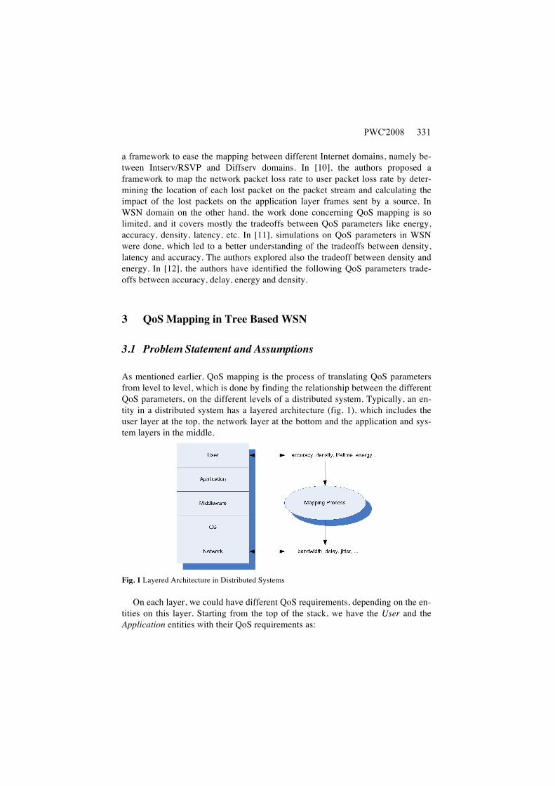
tity in a distributed system has a layered architecture (fig. 1), which includes the

user layer at the top, the network layer at the bottom and the application and sys-

tem layers in the middle.

Fig. 1 Layered Architecture in Distributed Systems

On each layer, we could have different QoS requirements, depending on the en-

tities on this layer. Starting from the top of the stack, we have the User and the

Application entities with their QoS requirements as:

PWC'2008 331

1. Accuracy: It could be seen as the difference between a set of values assumed as

the real values, and the value sensed by the network. Clearly, the number of active

nodes in the network has a big impact on this amount of error: when the number of

active nodes is increased, the computed error decreases.

2. Density: is the number of active nodes in the network divided by the volume.

As mentioned above, network density has a direct impact on accuracy.

3. Energy: energy consumption is one of the most vital issues in WSN. Due to

their small size, sensors suffer from their scarce resources like energy or memory.

Thus, energy is usually an important QoS requirement for WSN users.

4. Lifetime: network lifetime could be seen as the duration for which a desired

QoS is maintained. It could be also seen as the time until the first node (or a subset

of nodes) fails, or runs out of energy.

When communication network is of concern, other QoS parameters are distin-

guished like bandwidth, delay, jitter, etc.

In order to guarantee a User level QoS, e.g. a certain amount of accuracy, we

may have to add (or wake up) a number of nodes, thus we should try to answer the

following questions: what does this amount of accuracy equals in terms of net-

work density? And what does this amount of density equals in terms of lower level

parameters (network level parameters) so that we can do the suitable reservations

on that level?

Thus there is need to translate User level QoS, to Network level QoS (e.g. the

bandwidth allocated for each node).

In the following, we discuss how user QoS requirements like accuracy and den-

sity in WSN, could be mapped into network QoS parameters like bandwidth. It

has been noticed that in order to change the amount of accuracy (say increasing

accuracy), we should add more nodes to the network (e.g. by turning them on),

thus changing the network density. Once density is changed, the amount of band-

width reserved for each node will change too.

In order to better understand the relationship between the density of a network

and the bandwidth reserved for each node, we took as a model for our case of

study, a tree-based clustered WSN, with a TDMA-based MAC protocol. Tree-

based clustered architectures are being widely used in WSN [13] because they are

easily scalable and because of their unidirectional flow model, from leaves (sensor

nodes) to the root (sink node).

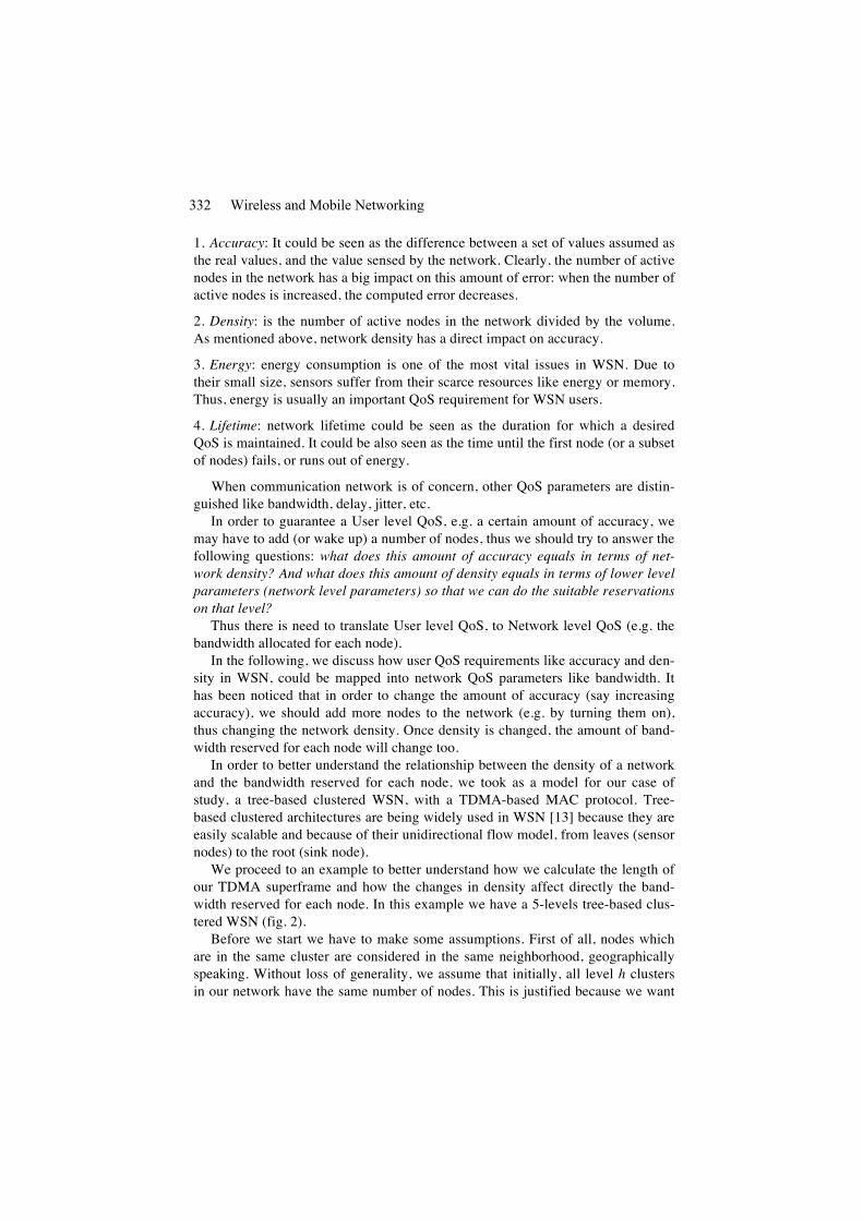
We proceed to an example to better understand how we calculate the length of

our TDMA superframe and how the changes in density affect directly the band-

width reserved for each node. In this example we have a 5-levels tree-based clus-

tered WSN (fig. 2).

Before we start we have to make some assumptions. First of all, nodes which

are in the same cluster are considered in the same neighborhood, geographically

speaking. Without loss of generality, we assume that initially, all level h clusters

in our network have the same number of nodes. This is justified because we want


to start our scenario by having a balanced network; nevertheless, our network

could evolve by adding or removing nodes from clusters, thus having eventually

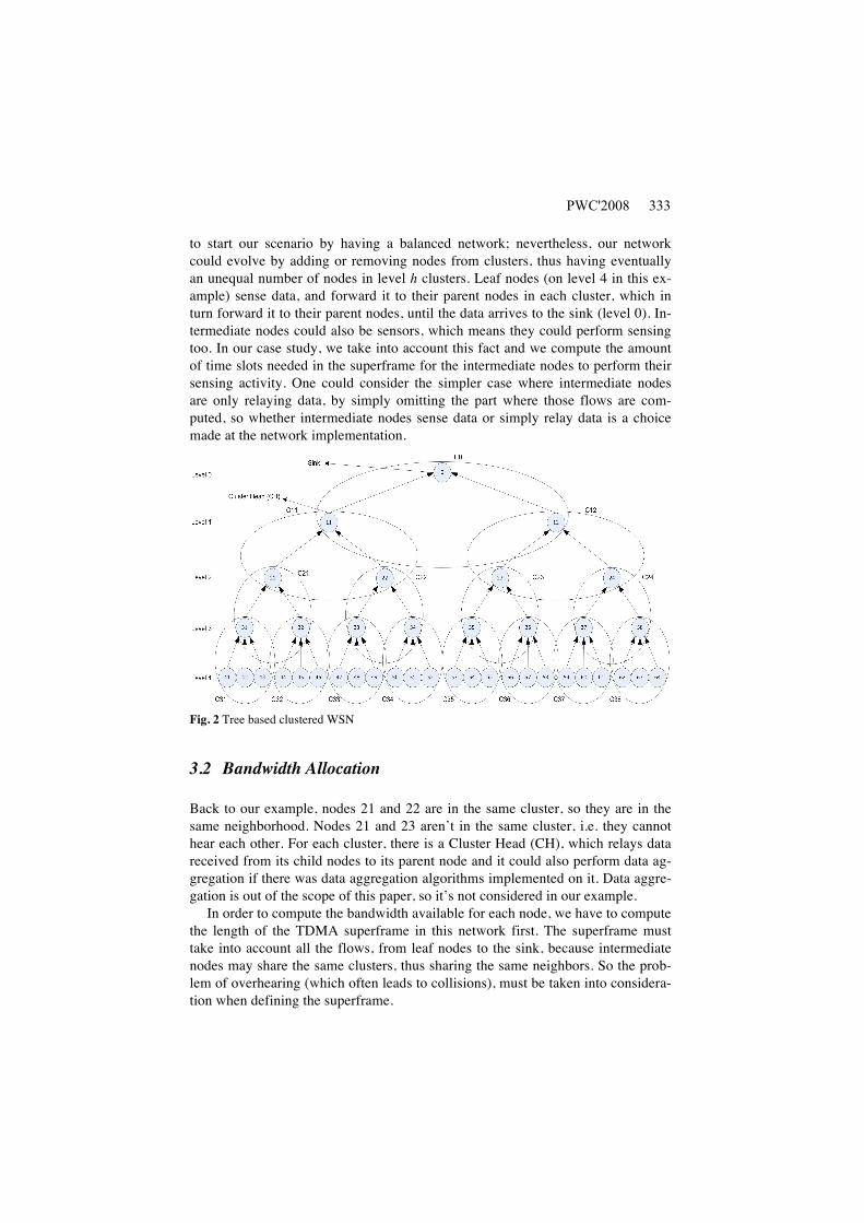
an unequal number of nodes in level h clusters. Leaf nodes (on level 4 in this ex-

ample) sense data, and forward it to their parent nodes in each cluster, which in

turn forward it to their parent nodes, until the data arrives to the sink (level 0). In-

termediate nodes could also be sensors, which means they could perform sensing

too. In our case study, we take into account this fact and we compute the amount

of time slots needed in the superframe for the intermediate nodes to perform their

sensing activity. One could consider the simpler case where intermediate nodes

are only relaying data, by simply omitting the part where those flows are com-

puted, so whether intermediate nodes sense data or simply relay data is a choice

made at the network implementation.

Fig. 2 Tree based clustered WSN

3.2 Bandwidth Allocation

Back to our example, nodes 21 and 22 are in the same cluster, so they are in the

same neighborhood. Nodes 21 and 23 aren’t in the same cluster, i.e. they cannot

hear each other. For each cluster, there is a Cluster Head (CH), which relays data

received from its child nodes to its parent node and it could also perform data ag-

gregation if there was data aggregation algorithms implemented on it. Data aggre-

gation is out of the scope of this paper, so it’s not considered in our example.

In order to compute the bandwidth available for each node, we have to compute

the length of the TDMA superframe in this network first. The superframe must

take into account all the flows, from leaf nodes to the sink, because intermediate

nodes may share the same clusters, thus sharing the same neighbors. So the prob-

lem of overhearing (which often leads to collisions), must be taken into considera-

tion when defining the superframe.

PWC'2008 333

We will proceed with the simplest case, and increase the problem complexity

until we reach the most general case.

i) First case: no simultaneous transmissions between clusters, sensing done

by leaf nodes only.

First, we consider the case of a WSN where only leaf nodes do sensing, therefore

all the intermediate nodes’ sensing flows are ignored. All simultaneous transmis-

sions between same level clusters and “3 hops away nodes” are also ignored in

this case.

The length of the TDMA superframe in a tree based clustered network with a

depth equal to H, is obtained by the means of the following formula:

(1)

where H denotes the depth of the tree and nh denotes the number of child nodes of

a CH on level h-1. This formula would be obvious if we observe the structure of

the superframe (fig. 3). As we notice, the superframe is composed of 4 equal parts:

24 time slots for transmitting 24 flows from leaf nodes, 24 time slots for level 3

nodes to transmit the incoming flows from leaf nodes, 24 time slots for level 2

nodes to transmit incoming flows from level 3 and 24 time slots for level 1 nodes

to transmit incoming flows from level 2 nodes.

Fig. 3 TDMA superframe (first case)

ii) Second case: simultaneous transmissions by same level clusters, sensing

done by leaf nodes only.

Now let us consider the case with simultaneous transmissions knowing that clus-

ters of the same level can transmit their respective flows on the same time slots

due to the fact that no overhearing could occur between separate clusters. Formula

(1) is thus reduced to:

(2)

This is depicted in (fig. 4). As we notice, flows from clusters C31 to C38 are

sent on the first, second and third time slots of the superframe because no over-

hearing could occur between those clusters. When the same rule is applied for

each of the levels, we obtain formula (2).


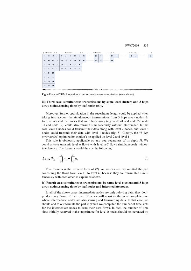
Fig. 4 Reduced TDMA superframe due to simultaneous transmissions (second case)

iii) Third case: simultaneous transmissions by same level clusters and 3 hops

away nodes, sensing done by leaf nodes only.

Moreover, further optimization in the superframe length could be applied when

taking into account the simultaneous transmissions from 3 hops away nodes. In

fact, we noticed that nodes that are 3 hops away (e.g. node 41 and node 22, node

31 and node 12), could also transmit simultaneously without interference. In that

case level 4 nodes could transmit their data along with level 2 nodes, and level 3

nodes could transmit their data with level 1 nodes (fig. 5). Clearly, the “3 hop

away nodes” optimization couldn’t be applied on level 2 and level 1.

This rule is obviously applicable on any tree, regardless of its depth H. We

could always transmit level h flows with level h-2 flows simultaneously without

interference. The formula would thus be the following:

(3)

This formula is the reduced form of (2). As we can see, we omitted the part

concerning the flows from level 3 to level H, because they are transmitted simul-

taneously with each other as explained above.

iv) Fourth case: simultaneous transmissions by same level clusters and 3 hops

away nodes, sensing done by leaf nodes and intermediate nodes.

In all of the above cases, intermediate nodes are only relaying data; they don’t

produce any flows of their own. Now we will consider the most complete case

where intermediate nodes are also sensing and transmitting data. In that case, we

should add to our formula the part in which we computed the number of time slots

for the intermediate nodes to send their own flows. In fact, the number of time

slots initially reserved in the superframe for level h nodes should be increased by

PWC'2008 335

Fig. 5 Optimized TDMA superframe with simultaneous transmissions for 3 hops away nodes

(third case)

Fig. 6 TDMA superframe in the complete case (fourth case)

Fh, which corresponds to the number of child intermediate nodes’ flows added to

level h nodes’ own flows:

(4)

In our example, the number of slots we should add to level 2 nodes (nodes 21

and 22) is: = n2 + n2 x n3 = 2 + 2 x 2 = 6 additional slots (3 for

each node). This is depicted in (fig. 6), where there are 9 slots reserved for node

21 instead of 6 slots in the previous case. In order to compute the total number of

slots added we should do the sum of Fh for every level defining the superframe

length, that is level 1 and level 2. So, the total number of slots added is:


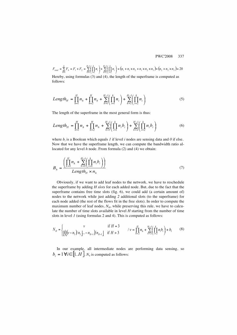
Hereby, using formulas (3) and (4), the length of the superframe is computed as

follows:

(5)

The length of the superframe in the most general form is thus:

(6)

where bi is a Boolean which equals 1 if level i nodes are sensing data and 0 if else.

Now that we have the superframe length, we can compute the bandwidth ratio al-

located for any level h node. From formula (2) and (4) we obtain:

(7)

Obviously, if we want to add leaf nodes to the network, we have to reschedule

the superframe by adding H slots for each added node. But, due to the fact that the

superframe contains free time slots (fig. 6), we could add (a certain amount of)

nodes to the network while just adding 2 additional slots (to the superframe) for

each node added (the rest of the flows fit in the free slots). In order to compute the

maximum number of leaf nodes, NH, while preserving this rule, we have to calcu-

late the number of time slots available in level H starting from the number of time

slots in level 1 (using formulas 2 and 4). This is computed as follows:

(8)

In our example, all intermediate nodes are performing data sensing, so

. N4 is computed as follows:

PWC'2008 337

€

N4

= nh

h= 2

4

∏ + ni

i= 2

k

∏ bi

+1

k= 2

3

∑ − n3

/ n3

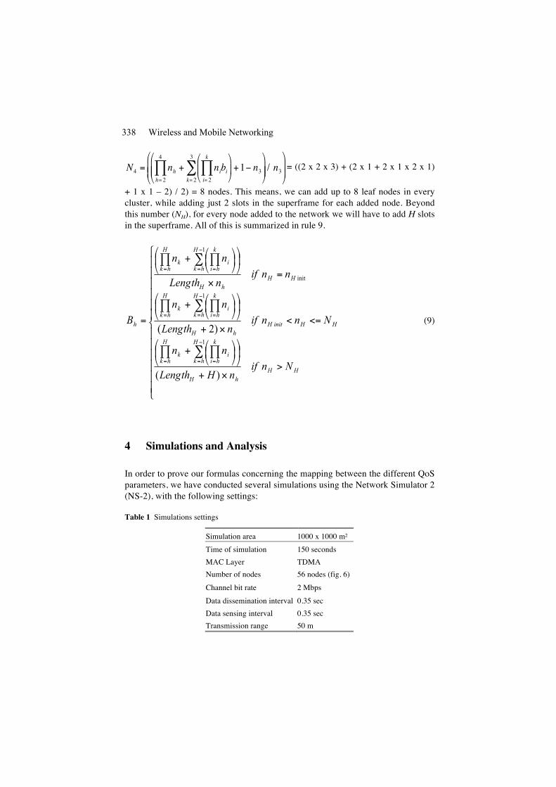
= ((2 x 2 x 3) + (2 x 1 + 2 x 1 x 2 x 1)

+ 1 x 1 – 2) / 2) = 8 nodes. This means, we can add up to 8 leaf nodes in every

cluster, while adding just 2 slots in the superframe for each added node. Beyond

this number (NH), for every node added to the network we will have to add H slots

in the superframe. All of this is summarized in rule 9.

(9)

4 Simulations and Analysis

In order to prove our formulas concerning the mapping between the different QoS

parameters, we have conducted several simulations using the Network Simulator 2

(NS-2), with the following settings:

Table 1 Simulations settings

Simulation area 1000 x 1000 m²

Time of simulation 150 seconds

MAC Layer TDMA

Number of nodes 56 nodes (fig. 6)

Channel bit rate 2 Mbps

Data dissemination interval 0.35 sec

Data sensing interval 0.35 sec

Transmission range 50 m


Below we discuss the main generic forms of relationships between QoS parame-

ters backed up by simulations.

4.1 Relationship Between Network Density and Bandwidth

The relationship between those two parameters is explained in the previous sec-

tion, where we proved that adding nodes to the network will decrease the band-

width reserved for each node by an amount computed using rule (9). In rule (9),

we presented three different formulas corresponding to three different cases, based

on the number of leaf nodes in each H cluster. Practically, it means that adding

one more node to the network, will slightly increase the superframe length (i.e.

slightly decrease the reporting frequency) thus reducing reserved bandwidth for

each node. On one hand we have gained accuracy by increasing network density,

and on the other we lost some accuracy while decreasing data freshness. A good

tradeoff between those values would be having NH leaf nodes in each cluster, us-

ing all the free slots in the superframe and thus increasing accuracy, while slightly

decreasing data freshness and bandwidth (2nd case in rule 9). Beyond this number,

reporting frequency will highly decrease and thus affecting the data freshness pa-

rameter; beside, the bandwidth for each node will also decrease leading for exam-

ple to the malfunctioning of the network (delay, jitter…).

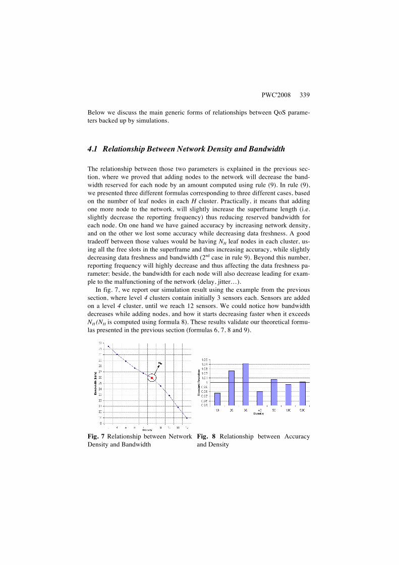
In fig. 7, we report our simulation result using the example from the previous

section, where level 4 clusters contain initially 3 sensors each. Sensors are added

on a level 4 cluster, until we reach 12 sensors. We could notice how bandwidth

decreases while adding nodes, and how it starts decreasing faster when it exceeds

NH (NH is computed using formula 8). These results validate our theoretical formu-

las presented in the previous section (formulas 6, 7, 8 and 9).

Fig. 7 Relationship between Network

Density and Bandwidth

Fig. 8 Relationship between Accuracy

and Density

PWC'2008 339

4.2 Relationship Between Accuracy and Network Density

Accuracy could be considered as the difference between the set of the real values

and the set of the sensed values. This difference could occur because of the physi-

cal nature of sensors, or their distance to the target. This could be represented by

the standard deviation, computed as follows:

(10)

where is the sensed value, is average value, and N is the number of sensed

samples. Obviously, we could minimize this amount of deviation by increasing the

network density, i.e. by increasing the number of nodes collecting data, a tech-

nique called data redundancy. That could be done either by adding nodes to the

cluster or by awaking sleeping nodes.

In our application (Temperature Sensing), we have varied the number of nodes

sensing temperature, in order to analyze the relationship between the measured ac-

curacy and the number of nodes sensing a certain phenomenon. Our sensed values

follow a Gaussian distribution, with an average temperature of 25°C, and a stan-

dard deviation of 1°C.

In fig. 9, we show how the standard deviation of the data samples converges

toward the theoretical deviation (of 1°C) as the network density increases.

The small amount of accuracy gained while moving from 100 sensors to 500

sensors for example, may raise the tradeoff issue between the gained accuracy and

the cost incurred.

4.3 Relationship Between Reporting Period, Network Density and

Packet Size

Reporting period or data freshness is in fact considered as another facet of accu-

racy. A fresher data (i.e. a shorter reporting period), corresponds to more accurate

results. Packet size also affects accuracy: a bigger packet carries more accurate

measurements.

Reporting period is directly related to the number of reporting nodes and it de-

pends also on the packet size. In this case, modifying one parameter could affect

the others. For example, in order to increase data freshness (i.e. decrease reporting

period), we will have to decrease the superframe length, by either removing time

slots (i.e. decreasing the number of nodes), or by decreasing the packet size al-


lowed for each node. In both cases, accuracy will be affected negatively. So there

is clearly a tradeoff to be done between those parameters.

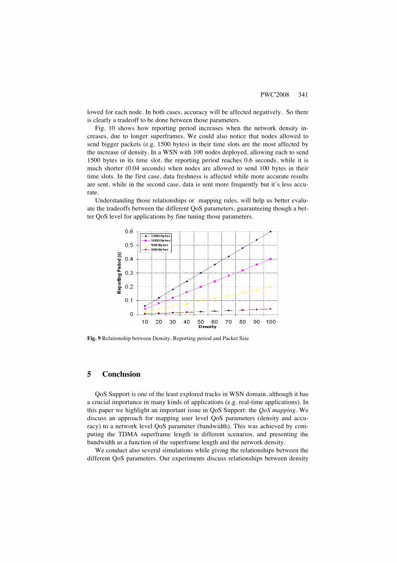
Fig. 10 shows how reporting period increases when the network density in-

creases, due to longer superframes. We could also notice that nodes allowed to

send bigger packets (e.g. 1500 bytes) in their time slots are the most affected by

the increase of density. In a WSN with 100 nodes deployed, allowing each to send

1500 bytes in its time slot, the reporting period reaches 0.6 seconds, while it is

much shorter (0.04 seconds) when nodes are allowed to send 100 bytes in their

time slots. In the first case, data freshness is affected while more accurate results

are sent, while in the second case, data is sent more frequently but it’s less accu-

rate.

Understanding those relationships or mapping rules, will help us better evalu-

ate the tradeoffs between the different QoS parameters, guaranteeing though a bet-

ter QoS level for applications by fine tuning those parameters.

Fig. 9 Relationship between Density, Reporting period and Packet Size

5 Conclusion

QoS Support is one of the least explored tracks in WSN domain, although it has

a crucial importance in many kinds of applications (e.g. real-time applications). In

this paper we highlight an important issue in QoS Support: the QoS mapping. We

discuss an approach for mapping user level QoS parameters (density and accu-

racy) to a network level QoS parameter (bandwidth). This was achieved by com-

puting the TDMA superframe length in different scenarios, and presenting the

bandwidth as a function of the superframe length and the network density.

We conduct also several simulations while giving the relationships between the

different QoS parameters. Our experiments discuss relationships between density

PWC'2008 341

and bandwidth, accuracy and density, and between data freshness, density and

packet size. One possible track we will try to explore in the future is to find the re-

lationships between other QoS parameters like between density and delay for ex-

ample. We will try also to investigate other kinds of MAC protocols like 802.11e.

References

1. S. Datta and T. Woody, Business 2.0 Magazine, February 2007 issue.

2. Technology Review Magazine (MIT), February 2003 issue.

3. G.J. Pottie and W.J. Kaiser: Wireless integrated network sensors. Communications of the

ACM (2000).

4. W. Masri and Z. Mammeri: Middleware for Wireless Sensor Networks: A Comparative

Analysis. In: Proceedings of the 2007 IFIP International Conference on Network and Parallel

Computing – workshops (NPC 2007), China (September 2007).

5. R. Iyer and L. Kleinrock: QoS Control for Sensor Networks. In: Proceedings of ICC 2003,

Alaska (May 2003)

6. J. Zhou and C. Mu: Density Domination of QoS Control with Localized Information in

Wireless Sensor Networks. In: Proceedings of the 6th International Conference on ITS Tele-

communications, China (June 2006)

7. J. Frolik: QoS Control for Random Access Wireless Sensor Networks. In: Proceedings of the

IEEE Wireless Communications and Networking Conference, USA (March 2004)

8. B. H. Liu, P. Ray, S. Jha: Mapping Distributed Application SLA to Network QoS Parame-

ters. In: Proceedings of the 10th International Conference on Telecommunications, Tahiti

(February 2003)

9. Z. Mammeri: Framework for Parameter Mapping to Provide End-to-End QoS Guarantees in

IntServ/DiffServ Architectures. In: Computer Communications, Volume 28, (June 2005)

10. M. Al-Kuwaiti, N. Kyriakopoulos, and S. Hussein: QoS Mapping: A Framework Model for

Mapping Network Loss to Application Loss. In: Proceedings of the 2007 IEEE International

Conference on Signal Processing and Communications, UAE (November 2007)

11. S. Tilak, N. B. Abu-Ghazaleh, W. Heinzelman: Infrastructure Tradeoffs for Sensor Net-

works. In: Proceedings of the 1st ACM International Workshop on Wireless Sensor Net-

works and Applications, USA (September 2002)

12. S. Adlakha, S. Ganeriwal, C. Schurgers, M. Srivastava: Poster Abstract: Density, Accuracy,

Delay and Lifetime Tradeoffs in Wireless Sensor Networks – A Multidimensional Design

Perspective. In: Proceedings of the ACM SenSys, USA (November 2003)

13. A. Koubaa, M. Alves, E. Tovar: Modeling and Worst-Case Dimensioning of Cluster-Tree

Wireless Sensor Networks. In: Proceedings of the 27th IEEE International Real-Time Sys-

tems Symposium, Brazil (December 2006).


On QoS Mapping in TDMA Based Wireless Sensor...

Documents

Transcript of On QoS Mapping in TDMA Based Wireless Sensor...