LUND UNIVERSITY

PO Box 117221 00 Lund+46 46-222 00 00

On mm-Wave Multi-path Clustering and Channel Modeling

Gustafson, Carl; Haneda, Katsuyuki; Wyne, Shurjeel; Tufvesson, Fredrik

Published in:IEEE Transactions on Antennas and Propagation

DOI:10.1109/TAP.2013.2295836

Published: 2014-01-01

Link to publication

Citation for published version (APA):Gustafson, C., Haneda, K., Wyne, S., & Tufvesson, F. (2014). On mm-Wave Multi-path Clustering and ChannelModeling. IEEE Transactions on Antennas and Propagation, 62(3), 1445-1455. DOI:10.1109/TAP.2013.2295836

General rightsCopyright and moral rights for the publications made accessible in the public portal are retained by the authorsand/or other copyright owners and it is a condition of accessing publications that users recognise and abide by thelegal requirements associated with these rights.

• Users may download and print one copy of any publication from the public portal for the purpose of privatestudy or research. • You may not further distribute the material or use it for any profit-making activity or commercial gain • You may freely distribute the URL identifying the publication in the public portalTake down policyIf you believe that this document breaches copyright please contact us providing details, and we will removeaccess to the work immediately and investigate your claim.

Download date: 25. Jun. 2018

1

On mm-Wave Multi-path Clustering andChannel Modeling

Carl Gustafson, Katsuyuki Haneda,Member, IEEE, Shurjeel Wyne,Senior Member, IEEE, andFredrik Tufvesson,Senior Member, IEEE

Abstract—Efficient and realistic mm-wave channel models areof vital importance for the development of novel mm-wavewireless technologies. Though many of the current 60 GHzchannel models are based on the useful concept of multi-pathclusters, only a limited number of 60 GHz channel measurementshave been reported in the literature for this purpose. Therefore,there is still a need for further measurement based analysesofmulti-path clustering in the 60 GHz band.

This paper presents clustering results for a double-directional60 GHz MIMO channel model. Based on these results, we derive amodel which is validated with measured data. Statistical clusterparameters are evaluated and compared with existing channelmodels. It is shown that the cluster angular characteristics areclosely related to the room geometry and environment, making itinfeasible to model the delay and angular domains independently.We also show that when using ray tracing to model the channel,it is insufficient to only consider walls, ceiling, floor and tables;finer structures such as ceiling lamps, chairs and bookshelvesneed to be taken into account as well.

Index Terms—Millimeter wave propagation, channel modeling,60 GHz WLAN, IEEE 802.11ad, IEEE 802.15.3c.

I. I NTRODUCTION

As the requirements for efficient and reliable wireless com-munications with high throughput are ever-increasing, novelwireless techniques have to be considered, and the availableradio spectrum has to be used efficiently in order to overcomespectrum shortage. Due to the large bandwidth of at least 5GHz available worldwide [1], the 60 GHz band is a promisingcandidate for short-range wireless systems that require veryhigh data rates. Efforts have already been made regardingstandardization by the IEEE 802.15.3c [2] and IEEE 802.11ad[3] working groups, and some commercial products are alreadyavailable on the market.

The propagation characteristics in the 60 GHz band are quitedifferent from those in the lower frequency bands commonlyused today for cellular communication. Assuming identicaltransmit powers and antenna gains, the received power at60 GHz is smaller than that at lower frequencies due to asmaller receive antenna aperture at 60 GHz. Furthermore,since the dimensions of typical shadowing objects are largein relation to the wavelength at 60 GHz, sharp shadow zonesare formed, making diffraction an insignificant propagationmechanism [4], Also, due to the high penetration loss of

C. Gustafson and F. Tufvesson are with the Department of Electrical andInformation Technology, Lund University, Sweden.

K. Haneda is with the Department of Radio Science and Engineering, AaltoUniversity, School of Science and Technology, Finland.

S. Wyne is with the Department of Electrical Engineering, COMSATSInstitute of Information Technology, Islamabad, Pakistan.

most materials at 60 GHz, multi-path components propagatingthrough walls or other objects typically have low power. Duetothese propagation characteristics, highly directional antennasor adaptive beam-forming techniques are required in order toestablish a reliable 60 GHz communication link [5].

As the potential benefits of systems operating in the 60GHz band are directly related to the propagation environmentcharacteristics, realistic and reliable channel models are ofvital importance for the design and development of novel 60GHz technologies. Furthermore, as beam forming techniquesare vital for many types of mm-wave communications, thechannel should ideally be modeled using a MIMO model thattakes the angular characteristics of the channel into account.

The IEEE802.11ad channel model is a MIMO model basedon a mixture of ray tracing and measurement-based statisticalmodeling techniques [6]. It is a cluster-based spatio-temporalchannel model that supports several different environments.The measurements for the IEEE802.11ad model were con-ducted using highly directional antennas that were steeredindifferent directions in order to evaluate and model the clusterparameters of 60 GHz channels.

Several recent studies are directly related to theIEEE802.11ad model and include theoretical investigationsregarding capacity [7], spatial diversity techniques [8] andbeamforming performance [9], as well as an extended modelfor human blockage in 60 GHz channels [10].

In this paper, we present measurement-based results fora double-directional 60 GHz MIMO channel model in aconference room environment. Statistical cluster parametersare evaluated and compared with existing 60 GHz channelmodels. The novel aspect of our proposed channel model isthe method by which it models the spatio-temporal propertiesof the clusters. We provide two different ways of modelingthe cluster spatio-temporal properties; one being stochasticand the other a semi-deterministic approach that is based onray-tracing. Most of the current 60 GHz directional analysesrely on measurements using highly directional antennas thatare mechanically steered [11] and sometimes also include raytracing results [6]. The results in this paper are based onmeasurements using the virtual antenna array technique. Thedouble-directional estimates for the multi-path components(MPCs) were obtained using the SAGE algorithm. This tech-nique can potentially offer an improved resolution of the MPCparameters compared with techniques based on mechanicallysteered high-gain antennas [6]. The clustering results were thenobtained using an automated clustering algorithm.

2

II. 60 GHZ RADIO CHANNEL AND ANTENNA

MEASUREMENTS

A. Measurement Environment

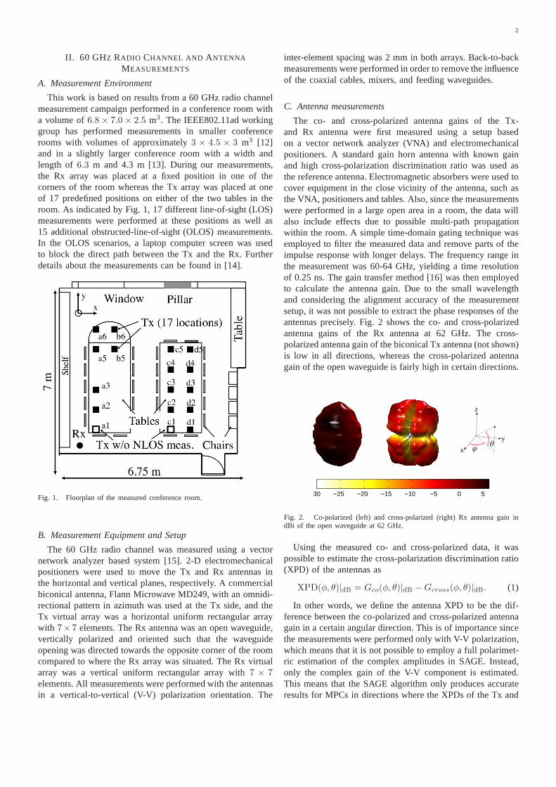
This work is based on results from a 60 GHz radio channelmeasurement campaign performed in a conference room witha volume of6.8× 7.0× 2.5 m3. The IEEE802.11ad workinggroup has performed measurements in smaller conferencerooms with volumes of approximately3 × 4.5 × 3 m3 [12]and in a slightly larger conference room with a width andlength of 6.3 m and 4.3 m [13]. During our measurements,the Rx array was placed at a fixed position in one of thecorners of the room whereas the Tx array was placed at oneof 17 predefined positions on either of the two tables in theroom. As indicated by Fig. 1, 17 different line-of-sight (LOS)measurements were performed at these positions as well as15 additional obstructed-line-of-sight (OLOS) measurements.In the OLOS scenarios, a laptop computer screen was usedto block the direct path between the Tx and the Rx. Furtherdetails about the measurements can be found in [14].

Fig. 1. Floorplan of the measured conference room.

B. Measurement Equipment and Setup

The 60 GHz radio channel was measured using a vectornetwork analyzer based system [15]. 2-D electromechanicalpositioners were used to move the Tx and Rx antennas inthe horizontal and vertical planes, respectively. A commercialbiconical antenna, Flann Microwave MD249, with an omnidi-rectional pattern in azimuth was used at the Tx side, and theTx virtual array was a horizontal uniform rectangular arraywith 7× 7 elements. The Rx antenna was an open waveguide,vertically polarized and oriented such that the waveguideopening was directed towards the opposite corner of the roomcompared to where the Rx array was situated. The Rx virtualarray was a vertical uniform rectangular array with7 × 7elements. All measurements were performed with the antennasin a vertical-to-vertical (V-V) polarization orientation. The

inter-element spacing was 2 mm in both arrays. Back-to-backmeasurements were performed in order to remove the influenceof the coaxial cables, mixers, and feeding waveguides.

C. Antenna measurements

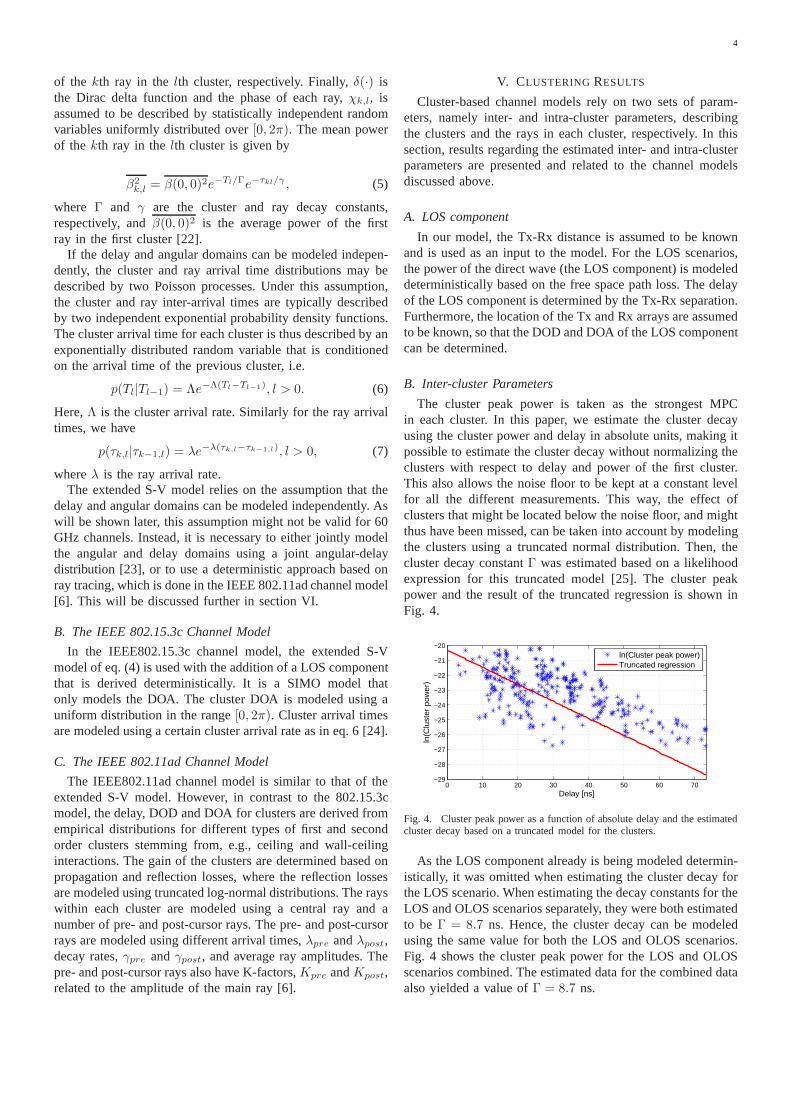
The co- and cross-polarized antenna gains of the Tx-and Rx antenna were first measured using a setup basedon a vector network analyzer (VNA) and electromechanicalpositioners. A standard gain horn antenna with known gainand high cross-polarization discrimination ratio was usedasthe reference antenna. Electromagnetic absorbers were used tocover equipment in the close vicinity of the antenna, such asthe VNA, positioners and tables. Also, since the measurementswere performed in a large open area in a room, the data willalso include effects due to possible multi-path propagationwithin the room. A simple time-domain gating technique wasemployed to filter the measured data and remove parts of theimpulse response with longer delays. The frequency range inthe measurement was 60-64 GHz, yielding a time resolutionof 0.25 ns. The gain transfer method [16] was then employedto calculate the antenna gain. Due to the small wavelengthand considering the alignment accuracy of the measurementsetup, it was not possible to extract the phase responses of theantennas precisely. Fig. 2 shows the co- and cross-polarizedantenna gains of the Rx antenna at 62 GHz. The cross-polarized antenna gain of the biconical Tx antenna (not shown)is low in all directions, whereas the cross-polarized antennagain of the open waveguide is fairly high in certain directions.

x

y

z

φθ

0 0.2 0.4 0.6 0.8 1

−30 −25 −20 −15 −10 −5 0 5

Fig. 2. Co-polarized (left) and cross-polarized (right) Rxantenna gain indBi of the open waveguide at 62 GHz.

Using the measured co- and cross-polarized data, it waspossible to estimate the cross-polarization discrimination ratio(XPD) of the antennas as

XPD(φ, θ)|dB = Gco(φ, θ)|dB −Gcross(φ, θ)|dB. (1)

In other words, we define the antenna XPD to be the dif-ference between the co-polarized and cross-polarized antennagain in a certain angular direction. This is of importance sincethe measurements were performed only with V-V polarization,which means that it is not possible to employ a full polarimet-ric estimation of the complex amplitudes in SAGE. Instead,only the complex gain of the V-V component is estimated.This means that the SAGE algorithm only produces accurateresults for MPCs in directions where the XPDs of the Tx and

3

Rx antennas are large [17]. In total, less than 5% of the totalnumber of MPCs in all scenarios were located in directionswere the XPD was lower than 20 dB.

III. M ULTI -PATH ESTIMATION AND CLUSTERING

A. The SAGE algorithm

The measured transfer functions are assumed to be correctlydescribed by a finite number of plane waves, i.e. multi-pathcomponents (MPCs). Each MPC is described by its complexamplitude, delay, direction of departure (DOD) and directionof arrival (DOA). In order to estimate these MPC parameters,the SAGE algorithm is used. A double-directional analysisusing SAGE based on the same measurements was previouslypresented in [18], and the reader is referred to that paper fordetails regarding the signal model for the analysis. This workimproves the SAGE estimates of [18] by employing a moredetailed model for the gain patterns of the antennas used in themeasurements. By taking the gain of the antennas into account,the estimated results describe the propagation channel.

The SAGE analysis was performed over an observationbandwidth of 200 MHz centered at 62 GHz with 26 equi-spaced frequency samples. The estimated MPCs can be usedto model the 2 GHz band from 61–63 GHz because the multi-path parameters do not change drastically over this frequencyband. This assertion is justified by the fact that neither thepower angular profiles [19], nor the SAGE estimates changedrastically when evaluated at center frequencies of 61, 62 and63 GHz.

B. Clustering Method

In this paper, a cluster is defined as a group of multi-pathcomponents having similar delays and directions of departureand arrival. The estimated MPCs are grouped into clustersusing the K-power-means algorithm wherein the multi-pathcomponent distance is used as a distance metric in parameterspace [20]. For the validation of the number of clusters, theKim-Parks index [21] was utilized. The Kim-Parks index,KP ,can be considered as a normalized version of the Davies-Bouldin index. It is calculated using an over- and under-partition measure function,vo andvu, that are normalized withrespect to the minimum and maximum number of clusters,Cmin andCmax,

KP (C) = vo(C) + vu(C). (2)

The optimal number of clusters,Copt, for a certain scenariois then given by

Copt = argminC

KP (C) , Cmin ≤ C ≤ Cmax. (3)

In practice, the largest number of clusters is set to be a numberthat is large enough to make sure that the correct number of

clusters is identified. For a more detailed description of theKim-Parks index, the reader is referred to [21]. The Kim-Parks index was chosen over the combined validation schemeas it produced consistent results that agreed better with thenumber of cluster identified based on a visual inspection.When using the Kim-Parks index, the number of identifiedclusters ranged from 6 to 12 in the LOS scenario and 8 to 12in the OLOS scenario. Fig. 3 show typical clustering resultsfor the direction of departure. Similar results were obtainedfor the direction of arrival. Each circle represents an MPC andthe colors indicate identified clusters and the radius of eachcircle is proportional to the power of each MPC. In order toget more consistent results in the LOS and OLOS scenarios,the clustering in the LOS scenarios are performed withoutincluding the LOS component. That way, the power levels aresimilar in both scenarios. It is possible to exclude the LOScomponent from the clustering since this component can betreated deterministically. The clustering results for theLOSand OLOS scenarios are very similar. The main differencesbetween the LOS and OLOS scenarios are

1) A strong LOS component present in the LOS scenario.2) A number of components are present in the OLOS

scenario that are diffracted around the computer screen.

−180

−90

0

90

180 00.2

0.40.6

0.81

x 10−7

90

45

0

−45

−90

Ele

vatio

n [d

eg]

Delay [s]Azimuth angle, [deg]

DOD

Fig. 3. Typical clustering result for the direction of departure.

IV. SURVEY OF 60 GHZ CHANNEL MODELS

A. The Extended Saleh-Valenzuela Model

Based on the clustering results, a number of statistical 60GHz channel model parameters can be derived. One of themost widely used channel models based on clusters is the ex-tended Saleh-Valenzuela model, where the impulse response,h, is given by Eq. (4). Here,βk,l is the complex amplitude ofthe kth ray (i.e. MPC) in thelth cluster andTl, Ωl andΨl

are the delay, DOA and DOD of thelth cluster, respectively.Similarly τk,l, ωk,l and ψk,l are the delay, DOA and DOD

h(t,Θrx,Θtx) =

L∑

l=0

Kl∑

k=0

βk,lejχklδ (t− Tl − τk,l) δ (Θrx − Ωl − ωk,l) δ (Θtx −Ψl − ψk,l) (4)

4

of the kth ray in thelth cluster, respectively. Finally,δ(·) isthe Dirac delta function and the phase of each ray,χk,l, isassumed to be described by statistically independent randomvariables uniformly distributed over[0, 2π). The mean powerof the kth ray in thelth cluster is given by

β2k,l = β(0, 0)2e−Tl/Γe−τkl/γ , (5)

where Γ and γ are the cluster and ray decay constants,respectively, andβ(0, 0)2 is the average power of the firstray in the first cluster [22].

If the delay and angular domains can be modeled indepen-dently, the cluster and ray arrival time distributions may bedescribed by two Poisson processes. Under this assumption,the cluster and ray inter-arrival times are typically describedby two independent exponential probability density functions.The cluster arrival time for each cluster is thus described by anexponentially distributed random variable that is conditionedon the arrival time of the previous cluster, i.e.

p(Tl|Tl−1) = Λe−Λ(Tl−Tl−1), l > 0. (6)

Here,Λ is the cluster arrival rate. Similarly for the ray arrivaltimes, we have

p(τk,l|τk−1,l) = λe−λ(τk,l−τk−1,l), l > 0, (7)

whereλ is the ray arrival rate.The extended S-V model relies on the assumption that the

delay and angular domains can be modeled independently. Aswill be shown later, this assumption might not be valid for 60GHz channels. Instead, it is necessary to either jointly modelthe angular and delay domains using a joint angular-delaydistribution [23], or to use a deterministic approach basedonray tracing, which is done in the IEEE 802.11ad channel model[6]. This will be discussed further in section VI.

B. The IEEE 802.15.3c Channel Model

In the IEEE802.15.3c channel model, the extended S-Vmodel of eq. (4) is used with the addition of a LOS componentthat is derived deterministically. It is a SIMO model thatonly models the DOA. The cluster DOA is modeled using auniform distribution in the range[0, 2π). Cluster arrival timesare modeled using a certain cluster arrival rate as in eq. 6 [24].

C. The IEEE 802.11ad Channel Model

The IEEE802.11ad channel model is similar to that of theextended S-V model. However, in contrast to the 802.15.3cmodel, the delay, DOD and DOA for clusters are derived fromempirical distributions for different types of first and secondorder clusters stemming from, e.g., ceiling and wall-ceilinginteractions. The gain of the clusters are determined basedonpropagation and reflection losses, where the reflection lossesare modeled using truncated log-normal distributions. Therayswithin each cluster are modeled using a central ray and anumber of pre- and post-cursor rays. The pre- and post-cursorrays are modeled using different arrival times,λpre andλpost,decay rates,γpre andγpost, and average ray amplitudes. Thepre- and post-cursor rays also have K-factors,Kpre andKpost,related to the amplitude of the main ray [6].

V. CLUSTERING RESULTS

Cluster-based channel models rely on two sets of param-eters, namely inter- and intra-cluster parameters, describingthe clusters and the rays in each cluster, respectively. In thissection, results regarding the estimated inter- and intra-clusterparameters are presented and related to the channel modelsdiscussed above.

A. LOS component

In our model, the Tx-Rx distance is assumed to be knownand is used as an input to the model. For the LOS scenarios,the power of the direct wave (the LOS component) is modeleddeterministically based on the free space path loss. The delayof the LOS component is determined by the Tx-Rx separation.Furthermore, the location of the Tx and Rx arrays are assumedto be known, so that the DOD and DOA of the LOS componentcan be determined.

B. Inter-cluster Parameters

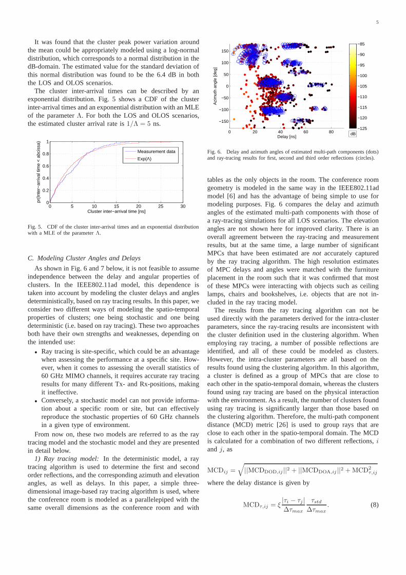
The cluster peak power is taken as the strongest MPCin each cluster. In this paper, we estimate the cluster decayusing the cluster power and delay in absolute units, making itpossible to estimate the cluster decay without normalizingtheclusters with respect to delay and power of the first cluster.This also allows the noise floor to be kept at a constant levelfor all the different measurements. This way, the effect ofclusters that might be located below the noise floor, and mightthus have been missed, can be taken into account by modelingthe clusters using a truncated normal distribution. Then, thecluster decay constantΓ was estimated based on a likelihoodexpression for this truncated model [25]. The cluster peakpower and the result of the truncated regression is shown inFig. 4.

0 10 20 30 40 50 60 70−29

−28

−27

−26

−25

−24

−23

−22

−21

−20

Delay [ns]

ln(C

lust

er p

ower

)

ln(Cluster peak power)Truncated regression

Fig. 4. Cluster peak power as a function of absolute delay andthe estimatedcluster decay based on a truncated model for the clusters.

As the LOS component already is being modeled determin-istically, it was omitted when estimating the cluster decayforthe LOS scenario. When estimating the decay constants for theLOS and OLOS scenarios separately, they were both estimatedto beΓ = 8.7 ns. Hence, the cluster decay can be modeledusing the same value for both the LOS and OLOS scenarios.Fig. 4 shows the cluster peak power for the LOS and OLOSscenarios combined. The estimated data for the combined dataalso yielded a value ofΓ = 8.7 ns.

5

It was found that the cluster peak power variation aroundthe mean could be appropriately modeled using a log-normaldistribution, which corresponds to a normal distribution in thedB-domain. The estimated value for the standard deviation ofthis normal distribution was found to be the 6.4 dB in boththe LOS and OLOS scenarios.

The cluster inter-arrival times can be described by anexponential distribution. Fig. 5 shows a CDF of the clusterinter-arrival times and an exponential distribution with an MLEof the parameterΛ. For both the LOS and OLOS scenarios,the estimated cluster arrival rate is1/Λ = 5 ns.

0 5 10 15 20 25 300

0.2

0.4

0.6

0.8

1

Cluster inter−arrival time [ns]

pr(I

nter

−ar

rival

tim

e <

abc

issa

)

Measurement data

Exp(Λ)

Fig. 5. CDF of the cluster inter-arrival times and an exponential distributionwith a MLE of the parameterΛ.

C. Modeling Cluster Angles and Delays

As shown in Fig. 6 and 7 below, it is not feasible to assumeindependence between the delay and angular properties ofclusters. In the IEEE802.11ad model, this dependence istaken into account by modeling the cluster delays and anglesdeterministically, based on ray tracing results. In this paper, weconsider two different ways of modeling the spatio-temporalproperties of clusters; one being stochastic and one beingdeterministic (i.e. based on ray tracing). These two approachesboth have their own strengths and weaknesses, depending onthe intended use:

• Ray tracing is site-specific, which could be an advantagewhen assessing the performance at a specific site. How-ever, when it comes to assessing the overall statistics of60 GHz MIMO channels, it requires accurate ray tracingresults for many different Tx- and Rx-positions, makingit ineffective.

• Conversely, a stochastic model can not provide informa-tion about a specific room or site, but can effectivelyreproduce the stochastic properties of 60 GHz channelsin a given type of environment.

From now on, these two models are referred to as the raytracing model and the stochastic model and they are presentedin detail below.

1) Ray tracing model: In the deterministic model, a raytracing algorithm is used to determine the first and secondorder reflections, and the corresponding azimuth and elevationangles, as well as delays. In this paper, a simple three-dimensional image-based ray tracing algorithm is used, wherethe conference room is modeled as a parallelepiped with thesame overall dimensions as the conference room and with

0 20 40 60 80

−150

−100

−50

0

50

100

150

Delay [ns]

Azi

mut

h an

gle

[deg

]

−125

−120

−115

−110

−105

−100

−95

−90

−85

dB

Fig. 6. Delay and azimuth angles of estimated multi-path components (dots)and ray-tracing results for first, second and third order reflections (circles).

tables as the only objects in the room. The conference roomgeometry is modeled in the same way in the IEEE802.11admodel [6] and has the advantage of being simple to use formodeling purposes. Fig. 6 compares the delay and azimuthangles of the estimated multi-path components with those ofa ray-tracing simulations for all LOS scenarios. The elevationangles are not shown here for improved clarity. There is anoverall agreement between the ray-tracing and measurementresults, but at the same time, a large number of significantMPCs that have been estimated arenot accurately capturedby the ray tracing algorithm. The high resolution estimatesof MPC delays and angles were matched with the furnitureplacement in the room such that it was confirmed that mostof these MPCs were interacting with objects such as ceilinglamps, chairs and bookshelves, i.e. objects that are not in-cluded in the ray tracing model.

The results from the ray tracing algorithm can not beused directly with the parameters derived for the intra-clusterparameters, since the ray-tracing results are inconsistent withthe cluster definition used in the clustering algorithm. Whenemploying ray tracing, a number of possible reflections areidentified, and all of these could be modeled as clusters.However, the intra-cluster parameters are all based on theresults found using the clustering algorithm. In this algorithm,a cluster is defined as a group of MPCs that are close toeach other in the spatio-temporal domain, whereas the clustersfound using ray tracing are based on the physical interactionwith the environment. As a result, the number of clusters foundusing ray tracing is significantly larger than those based onthe clustering algorithm. Therefore, the multi-path componentdistance (MCD) metric [26] is used to group rays that areclose to each other in the spatio-temporal domain. The MCDis calculated for a combination of two different reflections, iandj, as

MCDij =√

||MCDDOD,ij ||2 + ||MCDDOA,ij ||2 +MCD2τ,ij

where the delay distance is given by

MCDτ,ij = ξ|τi − τj |∆τmax

τstd∆τmax

. (8)

6

Here, ∆τmax = maxij|τi − τj |, and τstd is the standarddevation of the delays. For our purposes,ξ = 3 was found tobe a suitable delay scaling factor. The MCD for angular datais given byMCDDOD/DOA,ij

= 12 |ai − aj |, where

ai = [sin(θi) cos(φi), sin(θi) sin(φi), cos(θi)]T

Before calculating the MCD, all rays are sorted with respectto their delays. Then, the MCD between the ray with theshortest delay and all other rays are calculated, and all rayswith a MCD < 0.25 are grouped together with the ray withthe shortest delay. Then, the same thing is done again for theremaining rays, until all rays have been assigned to a group.The cluster delays and angles are then determined as the delayand angles of the rays with the shortest delays in each group.

2) Stochastic model: In the stochastic model, the clusterangles are modeled using conditional probabilities. The clusterdelays,Tk, are are modeled based on exponentially distributedcluster inter-arrival times. Then, the cluster elevation angles,Θk are determined using a joint pdf for the elevation anglesconditioned on the cluster delay, i.e.,

f(Tk,Θk) = f(Θk|Tk)f(Tk), (9)

wheref(Θk|Tk) is the conditional cluster elevation pdf andf(Tk) is the marginal pdf for the cluster delay. This conditionalpdf is determined empirically by considering the possibleelevation angles for first and second order reflections in a roomwith certain dimensions. The idea is that this conditional pdfshould reflect upon the possible elevation angles for severaldifferent scenarios, with the Tx and Rx placed at differentheight. Here, we note that this paper only includes measuredresults for a single height of the Tx and Rx arrays. However,for the conditional pdf, we consider hypothetical scenarioswhere the Tx is located at a table at different heights,h1,varying from 5-40 cm above the table, emulating a laptop ora similar device. The Rx is located at heights,h2, varyingfrom 5 cm above the table height up to 5 cm from the ceiling,thereby emulating a device such as a DVD-player, projectoror internet access point.

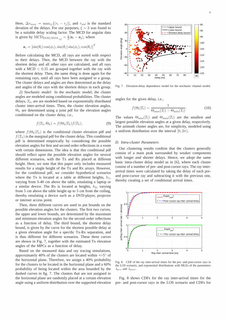
Then, three different curves are used to put bounds on thepossible elevation angles for the clusters. The first two curves,the upper and lower bounds, are determined by the maximumand minimum elevation angles for the second order reflectionsas a function of delay. The third bound, the shortest delaybound, is given by the curve for the shortest possible delay ata given elevation angle for a specific Tx-Rx separation, andis thus different for different scenarios. These three curvesare shown in Fig. 7, together with the estimated Tx elevationangles of the MPCs as a function of delay.

Based on the measured data and ray tracing simulations,approximately 40% of the clusters are located within +/-5 ofthe horizontal plane. Therefore, we assign a 40% probabilityfor the clusters to be located in the horizontal plane and a 60%probability of being located within the area bounded by thedashed curves in fig. 7. The clusters that are not assigned tothe horizontal plane are randomly placed at a certain elevationangle using a uniform distribution over the supported elevation

0 10 20 30 40 50 60 70 80−90

−60

−30

0

30

60

90

Delay [ns]

Ele

vatio

n an

gle

[deg

]

−125

−120

−115

−110

−105

−100

−95

−90

−85Upper boundLower boundShortest delay bound

dB

Fig. 7. Elevation-delay dependence model for the stochastic channel model.

angles for the given delay, i.e.,

f(Θl|Tl) =1

Θmax(Tl)−Θmin(Tl). (10)

The valuesΘmin(Tl) and Θmax(Tl) are the smallest andlargest possible elevation angles at a given delay, respectively.The azimuth cluster angles are, for simplicity, modeled usinga uniform distribution over the interval[0, 2π).

D. Intra-cluster Parameters

Our clustering results confirm that the clusters generallyconsist of a main peak surrounded by weaker componentswith longer and shorter delays. Hence, we adopt the samebasic intra-cluster delay model as in [6], where each clusterconsist of a number of pre- and post-cursor rays. The ray inter-arrival times were calculated by taking the delay of each pre-and post-cursor ray and subtracting it with the previous one,thereby creating a set of conditional arrival times.

0 1 2 3 4 50

0.5

1

0 1 2 3 4 50

0.5

1

Ray inter−arrival time [ns]

pr(R

ay in

ter−

arriv

al r

ate

< a

bcis

sa)

Exp(λpost

)

Post−cursor ray inter−arrival times

Exp(λpre

)

Pre−cursor ray inter−arrival times

Fig. 8. CDF of the ray inter-arrival times for the pre- and post-cursor rays inthe LOS scenario, and exponential distributions with MLEs of the parametersλpre andλpost.

Fig. 8 shows CDFs for the ray inter-arrival times for thepre- and post-cursor rays in the LOS scenario and CDFs for

7

exponential distributions with MLEs of the rate parametersλpre andλpost.

Next, the mean ray decay rates and K-factors for thepre- and post-cursor rays,γpre, γpost, Kpre andKpost, werecalculated by normalizing each ray with respect to the delayand mean amplitude of each associated cluster and performinga linear regression.

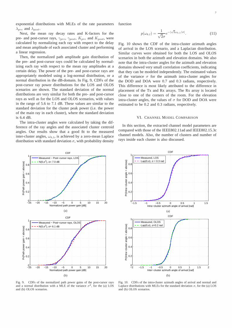
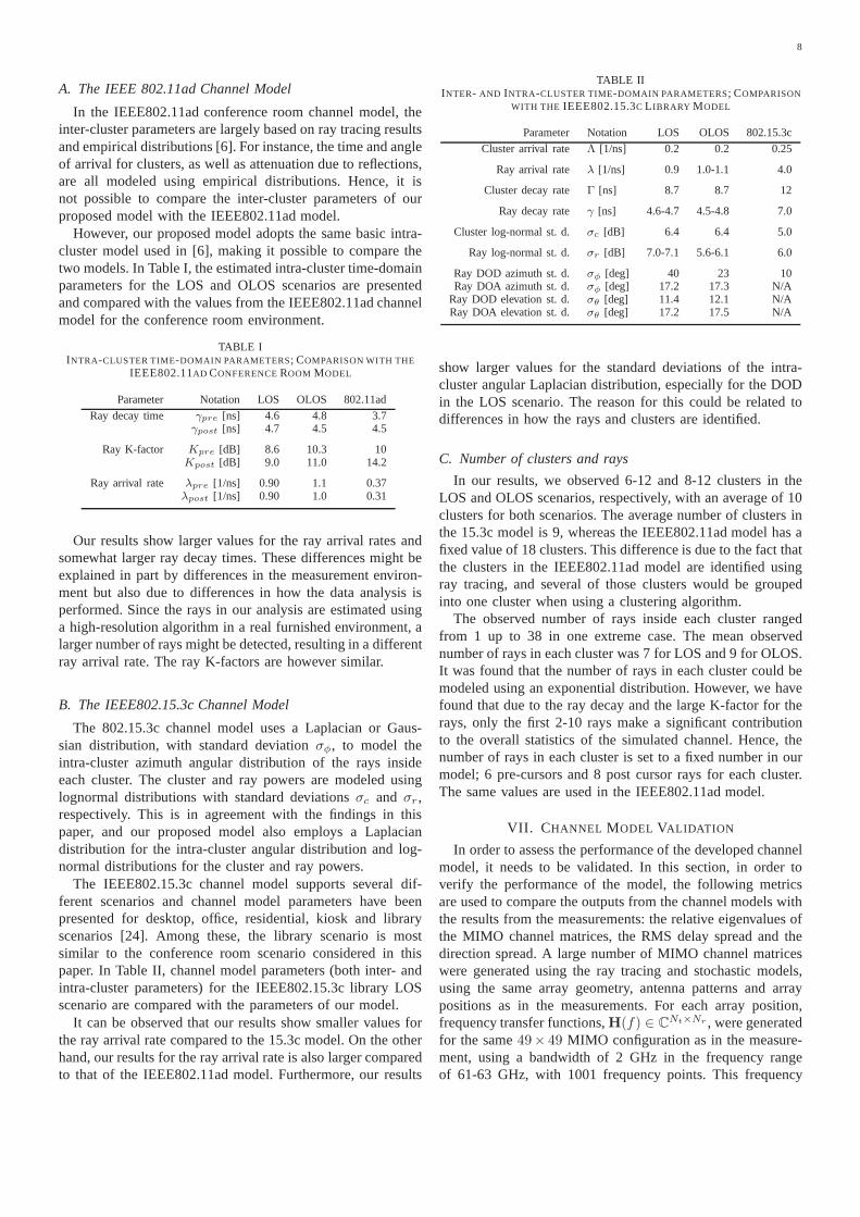
Then, the normalized path amplitude gain distribution ofthe pre- and post-cursor rays could be calculated by normal-izing each ray with respect to the mean ray amplitudes at acertain delay. The power of the pre- and post-cursor rays areappropriately modeled using a log-normal distribution, oranormal distribution in the dB-domain. In Fig. 9, CDFs of thepost-cursor ray power distributions for the LOS and OLOSscenarios are shown. The standard deviation of the normaldistributions are very similar for both the pre- and post-cursorrays as well as for the LOS and OLOS scenarios, with valuesin the range of 5.6 to 7.1 dB. These values are similar to thestandard deviation for the cluster peak power (i.e. the powerof the main ray in each cluster), where the standard deviationis 6.4 dB.

The intra-cluster angles were calculated by taking the dif-ference of the ray angles and the associated cluster centroidangles. Our results show that a good fit to the measuredinter-cluster angles,ωk,l, is achieved by a zero-mean Laplacedistribution with standard deviationσ, with probability density

−25 −20 −15 −10 −5 0 5 10 15 200

0.2

0.4

0.6

0.8

1

Normalized path power gain [dB]

Pr(

Pat

h po

wer

gai

n <

abc

issa

)

CDF

Measured − Post−cursor rays, LOS

N(0,σ2), σ= 7.0 dB

(a)

−25 −20 −15 −10 −5 0 5 10 15 200

0.2

0.4

0.6

0.8

1

Normalized path power gain [dB]

Pr(

Pat

h po

wer

gai

n <

abc

issa

)

CDF

Measured − Post−cursor rays, OLOS

N(0,σ2), σ= 6.1 dB

(b)

Fig. 9. CDFs of the normalized path power gains of the post-cursor raysand a normal distribution with a MLE of the varianceσ2, for the (a) LOSand (b) OLOS scenarios.

function

p(ωk,l) =1√2σe−|

√2ωk,l/σ|. (11)

Fig. 10 shows the CDF of the intra-cluster azimuth anglesof arrival in the LOS scenario, and a Laplacian distribution.Similar curves were obtained for both the LOS and OLOSscenarios in both the azimuth and elevation domains. We alsonote that the intra-cluster angles for the azimuth and elevationdomains showed very small correlation coefficients, indicatingthat they can be modeled independently. The estimated valuesof the varianceσ for the azimuth intra-cluster angles forthe DOD and DOA were 0.7 and 0.3 radians, respectively.This difference is most likely attributed to the differenceinplacement of the Tx and Rx arrays. The Rx array is locatedclose to one of the corners of the room. For the elevationintra-cluster angles, the values ofσ for DOD and DOA wereestimated to be 0.2 and 0.3 radians, respectively.

VI. CHANNEL MODEL COMPARISON

In this section, the extracted channel model parameters arecompared with those of the IEEE802.11ad and IEEE802.15.3cchannel models. Also, the number of clusters and number ofrays inside each cluster is also discussed.

−1.5 −1 −0.5 0 0.5 1 1.50

0.2

0.4

0.6

0.8

1

Intra−cluster azimuth angle of arrival [rad]

Pr(

Intr

a−cl

uste

r an

gle

< a

bcis

sa)

CDF

Measured, LOSLap(0,σ), σ = 0.3 rad

(a)

−2 −1.5 −1 −0.5 0 0.5 1 1.5 20

0.2

0.4

0.6

0.8

1

Inter−cluster azimuth angle of arrival [rad]

Pr(

Intr

a−cl

uste

r an

gle

< a

bcis

sa)

CDF

Measured, OLOSLap(0,σ), σ=0.2 rad

(b)

Fig. 10. CDFs of the intra-cluster azimuth angles of arrivaland normal andLaplace distributions with MLEs for the standard deviationσ, for the (a) LOSand (b) OLOS scenarios.

8

A. The IEEE 802.11ad Channel Model

In the IEEE802.11ad conference room channel model, theinter-cluster parameters are largely based on ray tracing resultsand empirical distributions [6]. For instance, the time andangleof arrival for clusters, as well as attenuation due to reflections,are all modeled using empirical distributions. Hence, it isnot possible to compare the inter-cluster parameters of ourproposed model with the IEEE802.11ad model.

However, our proposed model adopts the same basic intra-cluster model used in [6], making it possible to compare thetwo models. In Table I, the estimated intra-cluster time-domainparameters for the LOS and OLOS scenarios are presentedand compared with the values from the IEEE802.11ad channelmodel for the conference room environment.

TABLE IINTRA-CLUSTER TIME-DOMAIN PARAMETERS; COMPARISON WITH THE

IEEE802.11AD CONFERENCEROOM MODEL

Parameter Notation LOS OLOS 802.11ad

Ray decay time γpre [ns] 4.6 4.8 3.7γpost [ns] 4.7 4.5 4.5

Ray K-factor Kpre [dB] 8.6 10.3 10Kpost [dB] 9.0 11.0 14.2

Ray arrival rate λpre [1/ns] 0.90 1.1 0.37λpost [1/ns] 0.90 1.0 0.31

Our results show larger values for the ray arrival rates andsomewhat larger ray decay times. These differences might beexplained in part by differences in the measurement environ-ment but also due to differences in how the data analysis isperformed. Since the rays in our analysis are estimated usinga high-resolution algorithm in a real furnished environment, alarger number of rays might be detected, resulting in a differentray arrival rate. The ray K-factors are however similar.

B. The IEEE802.15.3c Channel Model

The 802.15.3c channel model uses a Laplacian or Gaus-sian distribution, with standard deviationσφ, to model theintra-cluster azimuth angular distribution of the rays insideeach cluster. The cluster and ray powers are modeled usinglognormal distributions with standard deviationsσc and σr ,respectively. This is in agreement with the findings in thispaper, and our proposed model also employs a Laplaciandistribution for the intra-cluster angular distribution and log-normal distributions for the cluster and ray powers.

The IEEE802.15.3c channel model supports several dif-ferent scenarios and channel model parameters have beenpresented for desktop, office, residential, kiosk and libraryscenarios [24]. Among these, the library scenario is mostsimilar to the conference room scenario considered in thispaper. In Table II, channel model parameters (both inter- andintra-cluster parameters) for the IEEE802.15.3c library LOSscenario are compared with the parameters of our model.

It can be observed that our results show smaller values forthe ray arrival rate compared to the 15.3c model. On the otherhand, our results for the ray arrival rate is also larger comparedto that of the IEEE802.11ad model. Furthermore, our results

TABLE IIINTER- AND INTRA-CLUSTER TIME-DOMAIN PARAMETERS; COMPARISON

WITH THE IEEE802.15.3C L IBRARY MODEL

Parameter Notation LOS OLOS 802.15.3c

Cluster arrival rate Λ [1/ns] 0.2 0.2 0.25

Ray arrival rate λ [1/ns] 0.9 1.0-1.1 4.0

Cluster decay rate Γ [ns] 8.7 8.7 12

Ray decay rate γ [ns] 4.6-4.7 4.5-4.8 7.0

Cluster log-normal st. d. σc [dB] 6.4 6.4 5.0

Ray log-normal st. d. σr [dB] 7.0-7.1 5.6-6.1 6.0

Ray DOD azimuth st. d. σφ [deg] 40 23 10Ray DOA azimuth st. d. σφ [deg] 17.2 17.3 N/A

Ray DOD elevation st. d. σθ [deg] 11.4 12.1 N/ARay DOA elevation st. d. σθ [deg] 17.2 17.5 N/A

show larger values for the standard deviations of the intra-cluster angular Laplacian distribution, especially for the DODin the LOS scenario. The reason for this could be related todifferences in how the rays and clusters are identified.

C. Number of clusters and rays

In our results, we observed 6-12 and 8-12 clusters in theLOS and OLOS scenarios, respectively, with an average of 10clusters for both scenarios. The average number of clustersinthe 15.3c model is 9, whereas the IEEE802.11ad model has afixed value of 18 clusters. This difference is due to the fact thatthe clusters in the IEEE802.11ad model are identified usingray tracing, and several of those clusters would be groupedinto one cluster when using a clustering algorithm.

The observed number of rays inside each cluster rangedfrom 1 up to 38 in one extreme case. The mean observednumber of rays in each cluster was 7 for LOS and 9 for OLOS.It was found that the number of rays in each cluster could bemodeled using an exponential distribution. However, we havefound that due to the ray decay and the large K-factor for therays, only the first 2-10 rays make a significant contributionto the overall statistics of the simulated channel. Hence, thenumber of rays in each cluster is set to a fixed number in ourmodel; 6 pre-cursors and 8 post cursor rays for each cluster.The same values are used in the IEEE802.11ad model.

VII. C HANNEL MODEL VALIDATION

In order to assess the performance of the developed channelmodel, it needs to be validated. In this section, in order toverify the performance of the model, the following metricsare used to compare the outputs from the channel models withthe results from the measurements: the relative eigenvalues ofthe MIMO channel matrices, the RMS delay spread and thedirection spread. A large number of MIMO channel matriceswere generated using the ray tracing and stochastic models,using the same array geometry, antenna patterns and arraypositions as in the measurements. For each array position,frequency transfer functions,H(f) ∈ CNt×Nr , were generatedfor the same49× 49 MIMO configuration as in the measure-ment, using a bandwidth of 2 GHz in the frequency rangeof 61-63 GHz, with 1001 frequency points. This frequency

9

range was chosen since 60 GHz wireless systems typicallyuse bandwidths as large as 2 GHz [2], [3]. Based on theseresults, we compare the statistical results from the model withthe measurements for the three chosen metrics.

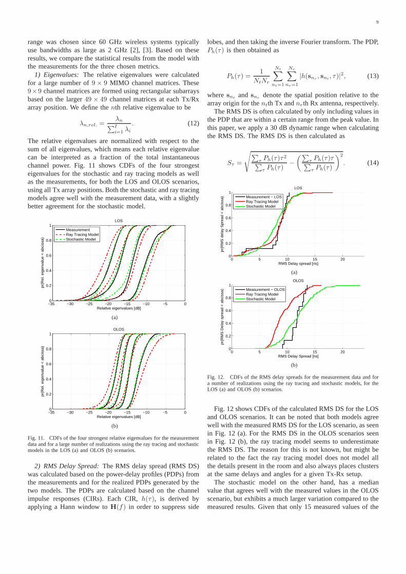
1) Eigenvalues: The relative eigenvalues were calculatedfor a large number of9 × 9 MIMO channel matrices. These9×9 channel matrices are formed using rectangular subarraysbased on the larger49 × 49 channel matrices at each Tx/Rxarray position. We define thenth relative eigenvalue to be

λn,rel. =λn

∑Ii=1 λi

. (12)

The relative eigenvalues are normalized with respect to thesum of all eigenvalues, which means each relative eigenvaluecan be interpreted as a fraction of the total instantaneouschannel power. Fig. 11 shows CDFs of the four strongesteigenvalues for the stochastic and ray tracing models as wellas the measurements, for both the LOS and OLOS scenarios,using all Tx array positions. Both the stochastic and ray tracingmodels agree well with the measurement data, with a slightlybetter agreement for the stochastic model.

−35 −30 −25 −20 −15 −10 −5 00

0.2

0.4

0.6

0.8

1

Relative eigenvalues [dB]

pr(R

el. e

igen

valu

e <

abc

issa

)

LOS

MeasurementRay Tracing ModelStochastic Model

(a)

−35 −30 −25 −20 −15 −10 −5 00

0.2

0.4

0.6

0.8

1

Relative eigenvalues [dB]

pr(R

el. e

igen

valu

e <

abc

issa

)

OLOS

(b)

Fig. 11. CDFs of the four strongest relative eigenvalues forthe measurementdata and for a large number of realizations using the ray tracing and stochasticmodels in the LOS (a) and OLOS (b) scenarios.

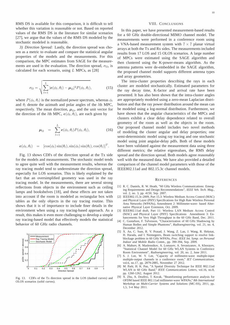
2) RMS Delay Spread: The RMS delay spread (RMS DS)was calculated based on the power-delay profiles (PDPs) fromthe measurements and for the realized PDPs generated by thetwo models. The PDPs are calculated based on the channelimpulse responses (CIRs). Each CIR,h(τ), is derived byapplying a Hann window toH(f) in order to suppress side

lobes, and then taking the inverse Fourier transform. The PDP,Ph(τ) is then obtained as

Ph(τ) =1

NtNr

Nt∑

nt=1

Nr∑

nr=1

|h(snr, snt

, τ)|2, (13)

wheresntand snr

denote the spatial position relative to thearray origin for thentth Tx andnrth Rx antenna, respectively.

The RMS DS is often calculated by only including values inthe PDP that are within a certain range from the peak value. Inthis paper, we apply a 30 dB dynamic range when calculatingthe RMS DS. The RMS DS is then calculated as

Sτ =

√

∑

τ Ph(τ)τ2∑

τ Ph(τ)−(∑

τ Ph(τ)τ∑

τ Ph(τ)

)2

. (14)

0 5 10 15 200

0.2

0.4

0.6

0.8

1

RMS Delay spread [ns]

pr(R

MS

del

ay S

prea

d <

abc

issa

)

LOS

Measurement − LOSRay Tracing ModelStochastic Model

(a)

0 5 10 15 200

0.2

0.4

0.6

0.8

1

RMS Delay Spread [ns]

pr(R

MS

Del

ay s

prea

d <

abc

issa

)

OLOS

Measurement − OLOSRay Tracing ModelStochastic Model

(b)

Fig. 12. CDFs of the RMS delay spreads for the measurement data and fora number of realizations using the ray tracing and stochastic models, for theLOS (a) and OLOS (b) scenarios.

Fig. 12 shows CDFs of the calculated RMS DS for the LOSand OLOS scenarios. It can be noted that both models agreewell with the measured RMS DS for the LOS scenario, as seenin Fig. 12 (a). For the RMS DS in the OLOS scenarios seenin Fig. 12 (b), the ray tracing model seems to underestimatethe RMS DS. The reason for this is not known, but might berelated to the fact the ray tracing model does not model allthe details present in the room and also always places clustersat the same delays and angles for a given Tx-Rx setup.

The stochastic model on the other hand, has a medianvalue that agrees well with the measured values in the OLOSscenario, but exhibits a much larger variation compared to themeasured results. Given that only 15 measured values of the

10

RMS DS is available for this comparison, it is difficult to tellwhether this variation is reasonable or not. Based on reportedvalues of the RMS DS in the literature for similar scenarios[27], we argue that the values of the RMS DS modeled by thestochastic modeled is reasonable.

3) Direction Spread: Lastly, the direction spread was cho-sen as a metric to evaluate and compare the statistical angularproperties of the models and the measurements. For thiscomparison, the MPC estimates from SAGE for the measure-ments are used in the evaluation. The direction spread,σΩ, iscalculated for each scenario, usingL MPCs, as [28]

σΩ =

√

√

√

√

L∑

l=1

|e(φl, θl)− µΩ|2P (φl, θl), (15)

whereP (φl, θl) is the normalized power spectrum, whereasφland θl denote the azimuth and polar angles of thelth MPC,respectively. The mean direction,µΩ, and the unit vector forthe direction of thelth MPC,e(φl, θl), are each given by

µΩ =

L∑

l=1

e(φl, θl)P (φl, θl), (16)

e(φl, θl) = [cos(φl) sin(θl), sin(φl) sin(θl), cos(θl)]T .

Fig. 13 shows CDFs of the direction spread at the Tx sidefor the models and measurements. The stochastic model tendsto agree quite well with the measurement results, whereas theray tracing model tend to underestimate the direction spread,especially for LOS scenarios. This is likely explained by thefact that an oversimplified geometry was used in the raytracing model. In the measurements, there are several strongreflections from objects in the environment such as ceilinglamps and bookshelves [18], and these effects are not takeninto account if the room is modeled as rectangular box withtables as the only objects in the ray tracing routine. Thisshows that it is of importance to include finer details in theenvironment when using a ray tracing-based approach. As aresult, this makes it even more challenging to develop a simpleray tracing-based model that effectively models the statisticalbehavior of 60 GHz radio channels.

0 0.1 0.2 0.3 0.4 0.5 0.6 0.7 0.8 0.9 10

0.2

0.4

0.6

0.8

1

Direction Spread

pr(D

ir. s

prea

d <

abc

issa

)

MeasurementRay Tracing ModelStochastic Model

Fig. 13. CDFs of the Tx direction spread in the LOS (dashed curves) andOLOS scenarios (solid curves).

VIII. C ONCLUSIONS

In this paper, we have presented measurement-based resultsfor a 60 GHz double-directional MIMO channel model. Themeasurements were performed in a conference room usinga VNA-based measurement system with7 × 7 planar virtualarrays at both the Tx and Rx sides. The measurements includedresults from 17 LOS and 15 OLOS scenarios. A large numberof MPCs were estimated using the SAGE algorithm andthen clustered using the K-power-means algorithm. As theantenna patterns were de-embedded in the SAGE algorithm,the proposed channel model supports different antenna typesand array geometries.

The intra-cluster properties describing the rays in eachcluster are modeled stochastically. Estimated parametersforthe ray decay time, K-factor and arrival rate have beenpresented. It has also been shown that the intra-cluster anglesare appropriately modeled using a zero-mean Laplacian distri-bution and that the ray power distribution around the mean canbe modeled using a log-normal distribution. Furthermore, wehave shown that the angular characteristics of the MPCs andclusters exhibit a clear delay dependence related to overallgeometry of the room as well as the objects in the room.Our proposed channel model includes two novel methodsof modeling the cluster angular and delay properties; onesemi-deterministic model using ray tracing and one stochasticmodel using joint angular-delay pdfs. Both of these modelshave been validated against the measurement data using threedifferent metrics; the relative eigenvalues, the RMS delayspread and the direction spread. Both models agree reasonablywell with the measured data. We have also provided a detailedcomparison of the channel model parameters with those of theIEEE802.11ad and 802.15.3c channel models.

REFERENCES

[1] R. C. Daniels, R. W. Heath, ”60 GHz Wireless Communications: Emerg-ing Requirements and Design Recommendations”,IEEE Veh. Tech. Mag.,vol. 2, no. 3, pp. 4150, Sep. 2007.

[2] IEEE802.15.3c-2009, Part 15.3: Wireless Medium AccessControl (MAC)and Physical Layer (PHY) Specifications for High Rate Wireless PersonalArea Networks (WPANs), Amendment 2: Millimeter-wave- based Alter-native Physical Layer Extension, Oct. 2009.

[3] IEEE802.11ad draft, Part 11: Wireless LAN Medium AccessControl(MAC) and Physical Layer (PHY) Specifications Amendment 3: En-hancements for Very High Throughput in the 60 GHz Band, Dec. 2011.

[4] C. Gustafson, F. Tufvesson, ”Characterization of 60 GHzShadowing byHuman Bodies and Simple Phantoms”,Radioengineering, vol. 21, no. 4,December 2012.

[5] X. An, C. Sum, R. V. Prasad, J. Wang, Z. Lan, J. Wang, R. Hekmat,H. Harada, and I. Niemegeers, Beam switching support to resolve link-blockage problem in 60 GHz WPANs,Proc. IEEE Int. Symp. on PersonalIndoor and Mobile Radio Comm., pp. 390-394, Sep. 2009.

[6] A. Maltsev, R. Maslennikov, A. Lomayev, A. Sevastyanov,A. Khorayev,”Statistical Channel Model for 60 GHz WLAN Systems in ConferenceRoom Environment”,Radioengineering, vol. 20, no. 2, June 2011.

[7] S. J. Lee, W. Y. Lee, ”Capacity of millimetre-wave multiple-inputmultiple-output channels in a conference room,”IET Communications,vol.6, no.17, pp. 2879-2885, November 27 2012.

[8] M. Park; H. K. Pan, ”A Spatial Diversity Technique for IEEE 802.11adWLAN in 60 GHz Band,” IEEE Communications Letters, vol.16, no.8,pp. 1260-1262, August 2012.

[9] X. Zhu, A. Doufexi, T. Kocak, ”Beamforming performance analysis forOFDM based IEEE 802.11ad millimeter-wave WPANs,”8th InternationalWorkshop on Multi-Carrier Systems and Solutions (MC-SS), 2011, pp.1,5, 3-4 May 2011.

11

[10] M. Jacob, S. Priebe, T. Kurner, M. Peter, M. Wisotzki, R.Felbecker, W.Keusgen, ”Extension and validation of the IEEE 802.11ad 60 GHz humanblockage model,”7th European Conference on Antennas and Propagation(EuCAP), pp. 2806-2810, 8-12 April 2013.

[11] H. Xu, V. Kukshya and T. S. Rappaport, Spatial and Temporal Charac-teristics of 60-GHz indoor Channels,IEEE Journal on Selected Areas inCommunications, Vol. 20, No. 3, April 2002.

[12] A. Maltsev, et. al., ”Channel Models for 60 GHz WLAN Systems” IEEE802.11-09/0334r8, May 2010.

[13] H. Sawada, S. Kato, K. Sato, H. Harada, et. al., ”Intra-cluster responsemodel and parameter for channel modeling at 60GHz (Part 3)”IEEE802.11-10/0112r1, Jan 2010.

[14] S. Wyne, K. Haneda, S. Ranvier, F. Tufvesson, and A. F. Molisch”Beamforming Effects on Measured mm-Wave Channel Characteristics”IEEE Transactions on Wireless Communications Vol:10, No. 11, 2011.

[15] S. Ranvier, M. Kyro, K. Haneda, C. Icheln and P. Vainikainen, VNA-based wideband 60 GHz MIMO channel sounder with 3D arrays,Proc.Radio Wireless Symp., pp. 308-311, San Diego, CA, Jan 2009.

[16] K.T. Selvan, ”A revisit of the reference antenna gain measurementmethod,” Proceedings of the 9th International Conference on Electro-magnetic Interference and Compatibility, (INCEMIC), pp.467-469, 23-24Feb. 2006

[17] M. Landmann, M. Kaske, R.S. Thoma, ”Impact of Incomplete andInaccurate Data Models on High Resolution Parameter Estimation inMultidimensional Channel Sounding,”IEEE Transactions on Antennasand Propagation , vol.60, no.2, pp.557-573, Feb. 2012

[18] C. Gustafson, F. Tufvesson, S. Wyne, K. Haneda, A. F. Molisch,”Directional analysis of measured 60 GHz indoor radio channels usingSAGE” IEEE 73rd Vehicular Technology Conference (VTC Spring),Budapest, Hungary, May 2011.

[19] K. Haneda, C. Gustafson, S. Wyne, ”60 GHz Spatial Radio Trans-mission: Multiplexing or Beamforming?”IEEE Trans. on Antennas andPropagation, vol.PP, no.99, 2013.

[20] N. Czink, P. Cera, J. Salo, E. Bonek, J.-P. Nuutinen, J. Ylitalo, ”Aframework for automatic clustering of parametric MIMO channel dataincluding path powers”,IEEE 64th Vehicular Technology Conference,pp.1-5, 25-28 Sept. 2006

[21] D.-J. Kim, Y.-W. Park, and D.-C. D.-J. Park, A Novel Validity Indexfor Determination of the Optimal Number of Clusters,IEICE Trans. Inf.& Syst., vol. E84-D, No. 2, pp. 281-285, 2001.

[22] Q. H. Spencer, B.D. Jeffs, M. A. Jensen, A. L. Swindlehurst, ”Modelingthe statistical time and angle of arrival characteristics of an indoormultipath channel,”IEEE Journal on Selected Areas in Communications,vol.18, no.3, pp.347-360, March 2000.

[23] C.-C. Chong, C.-M. Tan, D. I. Laurenson, S. McLaughlin,M. A. Beach,A. R. Nix, ”A New Statistical Wideband Spatio-Temporal Model for5 GHz Band WLAN Systems”,IEEE Journal on Selected Areas inCommunications, Vol. 21, No. 2, Feb. 2003.

[24] S-K. Yong, et al., TG3c channel modeling sub-commitee final report,IEEE Techn. Rep.,15-07-0584-01-003c, Mar. 2007.

[25] C. Gustafson, D. Bolin, F. Tufvesson, ”Modeling the cluster decayin mm-Wave channels”,8th European Conference on Antennas andPropagation (EuCAP), Hague, 6-11 April, 2014.

[26] N. Czink, P. Cera, J. Salo, E. Bonek, J.-P. Nuutinen and J. Ylitalo,”Improving clustering performance using multipath component distance”,Electronics Letters, 5th Jan. 2006 Vol. 42 No. 1.

[27] S.-K. Yong, P. Xia, A. Valdes-Garcia, ”60 GHz Technology for GbpsWLAN and WPAN: From Theory to Practice”,Wiley, 2011.

[28] B. H. Fleury, ”First- and second-order characterization of directiondispersion and space selectivity in the radio channel”,IEEE Transactionson Information Theory, vol. 46, pp. 2027 - 2044, September 2000.

Carl Gustafson received the M.Sc. degree in elec-trical engineering from Lund University, Lund, Swe-den, where he is currently working toward the Ph.D.degree at the Department of Electrical and Informa-tion Technology.

His main research interests include channel mea-surements and modeling for 60 GHz and millimeter-wave wireless systems. Other research interests in-clude antenna design, electromagnetic wave propa-gation as well as MIMO and UWB systems.

Katsuyuki Haneda (S’03-M’07) received the Doc-tor of Engineering from the Tokyo Institute of Tech-nology, Tokyo, Japan, in 2007.

Having served as a post-doctoral researcher at theSMARAD Centre of Excellence in the Aalto Uni-versity (former Helsinki University of Technology)School of Electrical Engineering, Espoo, Finland,Dr. Haneda is presently holding an assistant profes-sorship in the Aalto University School of ElectricalEngineering. Dr. Haneda was the recipient of thebest paper award of the antennas and propagation

track in the IEEE 77th Vehicular Technology Conference (VTC2013-Spring),Dresden, Germany, and of the best propagation paper award inthe 7th Euro-pean Conference on Antennas and Propagation (EuCAP2013), Gothenburg,Sweden. He also received the Student Paper Award presented at the 7thInternational Symposium on Wireless Personal Multimedia Communications(WPMC ’04).

Dr. Haneda has been serving as an associate editor for the IEEE Trans-actions on Antennas and Propagation since 2012 and as an editor for theAntenna Systems and Channel Characterization Area of the IEEE Transactionson Wireless Communications since 2013. He also served as a co-chair of thetopical working group on indoor environment in the EuropeanCOST ActionIC1004 Cooperative radio communications for green smart environments fortwo years during 2011-2013. His current research activity focuses on high-frequency radios such as millimeter-wave and beyond, wireless for medicalscenario, radio wave propagation prediction, and in-band full-duplex radiotechnologies.

Shurjeel Wyne (S’02-M’08-SM’13) received hisPh.D. from Lund University, Sweden in March 2009.Between April 2009 and April 2010, he was aPost-Doctoral Research Fellow funded by the High-Speed Wireless Centre at Lund University. SinceJune 2010 he holds an Assistant Professorship at theDepartment of Electrical Engineering at COMSATSInstitute of Information Technology, Islamabad, Pak-istan.

Dr. Wyne is a Co-recipient of the best paperaward of the Antennas and Propagation Track in

the IEEE 77th Vehicular Technology Conference (VTC2013-Spring), heldin Dresden, Germany. He has served as a Technical Program Committeemember for various international conferences, including most recently theIEEE International Conference on Communications, (ICC 2013), a flagshipconference of the IEEE Communications Society.

Dr Wynes research interests are in the area of wireless communications inparticular wireless channel measurements and modeling, 60GHz Communi-cations, relay networks, and Multiple-input Multiple-output (MIMO) systems.

Fredrik Tufvesson received his Ph.D. in 2000 fromLund University in Sweden. After almost two yearsat a startup company, Fiberless Society, he is nowassociate professor at the department of Electricaland Information Technology, Lund University. Hismain research interests are channel measurementsand modeling for wireless communication, includingchannels for both MIMO and UWB systems. Besidethis, he also works on distributed antenna systemsand radio based positioning.