On-line self-learning PID controller design of SSSC...
22
Turk J Elec Eng & Comp Sci (2013) 21: 980 – 1001 c ⃝ T ¨ UB ˙ ITAK doi:10.3906/elk-1112-49 Turkish Journal of Electrical Engineering & Computer Sciences http://journals.tubitak.gov.tr/elektrik/ Research Article On-line self-learning PID controller design of SSSC using self-recurrent wavelet neural networks Soheil GANJEFAR, * Mojtaba ALIZADEH Department of Electrical Engineering, Bu-Ali Sina University, Hamedan, Iran Received: 13.12.2011 • Accepted: 29.01.2012 • Published Online: 03.06.2013 • Printed: 24.06.2013 Abstract: Conventionally, FACTS devices employ a proportional-integral (PI) controller as a supplementary controller. However, the conventional PI controller has many disadvantages. The present paper aims to propose an on-line self- learning PI-derivative (PID) controller design of a static synchronous series compensator for power system stability enhancement and to overcome the PI controller problems. Unlike the PI controllers, the proposed PID controller has a local nature because of its powerful adaption process, which is based on the back-propagation (BP) algorithm that is carried out through an adaptive self-recurrent wavelet neural network identifier (ASRWNNI). In fact, the PID controller parameters are updated in on-line mode using the BP algorithm based on the information provided by the ASRWNNI, which is a powerful and fast-acting identifier thanks to its local nature, self-recurrent structure, and stable training algorithm with adaptive learning rates based on the discrete Lyapunov stability theorem. The proposed control scheme is applied to a 2-machine, 2-area power system under different operating conditions and disturbances to demonstrate its effectiveness and robustness. Later on, the design problem is extended to a 4-machine, 2-area benchmark system and the results show that the interarea modes of the oscillations are well damped with the proposed approach. Key words: Adaptive control, flexible AC transmission systems, power system control, power system stability, self- recurrent wavelet neural networks 1. Introduction Power systems can be studied as highly nonlinear large-scale dynamic systems [1]. Electromechanical oscillations occur when the power system is subjected to disturbances. Power system stabilizers (PSSs) are conventionally employed for power system oscillation damping. However, they have manydisadvantages; they can be adversely affected by the voltage profile while the system is operating at a leading power factor. Moreover, during a severe disturbance, their suppressing ability may be degraded [2,3]. The recent development of power electronics has attracted more attention to the use of flexible AC transmission system (FACTS) devices in power systems with the aim of damping the oscillations and improving the dynamic stability of the power system [4–11]. The suitably controlled FACTS devices can provide good damping to both the interarea and the local mode oscillations of a multimachine power system. Conventionally, FACTS devices employ a proportional-integral (PI) controller as a supplementary con- troller [12]. The PI controller is used in a wide range of industrial applications due to its simple structure and low cost. However, the PI-type controller has many disadvantages, which are more highlighted when the controlled object is highly nonlinear. In this situation, the PI controller is almost a deficient controller, and * Correspondence: s [email protected] 980
Transcript of On-line self-learning PID controller design of SSSC...

Turk J Elec Eng & Comp Sci
(2013) 21: 980 – 1001
c⃝ TUBITAK
doi:10.3906/elk-1112-49
Turkish Journal of Electrical Engineering & Computer Sciences
http :// journa l s . tub i tak .gov . t r/e lektr ik/
Research Article
On-line self-learning PID controller design of SSSC using self-recurrent wavelet
neural networks
Soheil GANJEFAR,∗ Mojtaba ALIZADEHDepartment of Electrical Engineering, Bu-Ali Sina University, Hamedan, Iran
Received: 13.12.2011 • Accepted: 29.01.2012 • Published Online: 03.06.2013 • Printed: 24.06.2013
Abstract: Conventionally, FACTS devices employ a proportional-integral (PI) controller as a supplementary controller.
However, the conventional PI controller has many disadvantages. The present paper aims to propose an on-line self-
learning PI-derivative (PID) controller design of a static synchronous series compensator for power system stability
enhancement and to overcome the PI controller problems. Unlike the PI controllers, the proposed PID controller has a
local nature because of its powerful adaption process, which is based on the back-propagation (BP) algorithm that is
carried out through an adaptive self-recurrent wavelet neural network identifier (ASRWNNI). In fact, the PID controller
parameters are updated in on-line mode using the BP algorithm based on the information provided by the ASRWNNI,
which is a powerful and fast-acting identifier thanks to its local nature, self-recurrent structure, and stable training
algorithm with adaptive learning rates based on the discrete Lyapunov stability theorem. The proposed control scheme
is applied to a 2-machine, 2-area power system under different operating conditions and disturbances to demonstrate its
effectiveness and robustness. Later on, the design problem is extended to a 4-machine, 2-area benchmark system and
the results show that the interarea modes of the oscillations are well damped with the proposed approach.
Key words: Adaptive control, flexible AC transmission systems, power system control, power system stability, self-
recurrent wavelet neural networks
1. Introduction
Power systems can be studied as highly nonlinear large-scale dynamic systems [1]. Electromechanical oscillations
occur when the power system is subjected to disturbances. Power system stabilizers (PSSs) are conventionally
employed for power system oscillation damping. However, they have many disadvantages; they can be adversely
affected by the voltage profile while the system is operating at a leading power factor. Moreover, during a severe
disturbance, their suppressing ability may be degraded [2,3].
The recent development of power electronics has attracted more attention to the use of flexible AC
transmission system (FACTS) devices in power systems with the aim of damping the oscillations and improving
the dynamic stability of the power system [4–11]. The suitably controlled FACTS devices can provide good
damping to both the interarea and the local mode oscillations of a multimachine power system.
Conventionally, FACTS devices employ a proportional-integral (PI) controller as a supplementary con-
troller [12]. The PI controller is used in a wide range of industrial applications due to its simple structure
and low cost. However, the PI-type controller has many disadvantages, which are more highlighted when the
controlled object is highly nonlinear. In this situation, the PI controller is almost a deficient controller, and
∗Correspondence: s [email protected]
980

GANJEFAR and ALIZADEH/Turk J Elec Eng & Comp Sci
its deficiency is mainly related to its tuning method as the first problem and its static nature as the second
problem.
To overcome the first problem, many different parameter tuning methods have been presented for PI/PI-
derivative (PID) controllers. A survey conducted up until 2002 was given in [13,14]. These methods are generally
modifications of the frequency response method proposed by Ziegler and Nichols [15]. Numerous analytical-
based works were also presented in order to tune the PI/PID parameters [16–18]. Robust and optimal control
methods were also proposed to design the PI/PID controllers [19–23]. Recently, as other alternatives to PID
tuning, modern heuristic optimization techniques such as simulated annealing [24], the evolutionary algorithm
[25], particle swarm optimization [26], and chaotic optimization [27] have been given much attention. Most of
these works propose a fixed-gain PI/PID controller with an unappealing static nature (the second problem).
The present paper aims to propose an on-line self-learning PID (OLSL-PID) controller for a static
synchronous series compensator (SSSC) for power system stability enhancement and to overcome the PI
controller problems. Unlike the PI controllers, the proposed PID controller has a local behavior because of
its powerful adaption process, which is based on the back-propagation (BP) algorithm. During the adaption
process, the Jacobian of the plant is also needed. Generally, 2 control strategies can be used to evaluate the
Jacobian, ‘direct adaptive control’ and ‘indirect adaptive control’. In this paper, it is calculated based on
the indirect adaptive control theory. An on-line identification algorithm is therefore required to evaluate the
Jacobian on-line.
Multilayer perceptron (MLP) networks, based on the gradient descent (GD) training algorithm with static
learning rates, are used by many researchers for the identification of synchronous generators [28–32]. However,
MLPs have some drawbacks due to their inherent characteristics [33]. They have a global nature due to their
use of the continued activation function. This global nature slows the speed of learning and results in the
essence of the local minimum. Recently, wavelet neural networks (WNNs), which absorb the advantages such
as the multiresolution of the wavelets and the learning of the MLP, were used to identify the nonlinear systems
[34–38]. The WNN is suitable for the approximation of unknown nonlinear functions with local nonlinearities
and fast variations because of its intrinsic properties of finite support and self-similarity [39]. Aside from these
advantages, the WNN has a shortcoming; due to its feed-forward network structure, it can only be used for
static problems. Hence, self-recurrent wavelet neural networks (SRWNNs), which combine such features as the
dynamics of the recurrent neural network and the fast convergence of the WNN, were proposed to identify the
nonlinear systems [33–40].
In this article a SRWNN is thus used as an identifier to adapt the PID controller parameters. Moreover,
the GD method using adaptive learning rates (ALRs) is applied to train all of the weights of the adaptive
SRWNN identifier (ASRWNNI). The proposed control scheme is applied to a 2-machine, 2-area power system
under different operating conditions and disturbances to demonstrate its effectiveness and robustness. Nonlinear
simulation results are also presented to highlight the promising features of the proposed controller. Later on,
the design problem is extended to a 4-machine, 2-area system and the results show that the interarea modes of
the oscillations are well damped with the proposed approach.
The reminder of the paper is organized as follows: the 2-machine, 2-area power system model is presented
in Section 2. The design of the OLSL-PID controller is described in Section 3. The SRWNN structure and
its application to the adaptive identifier design are presented in Section 4. The convergence analysis for the
ASRWNNI is provided in Section 5. The simulation results are discussed in Section 6. Section 7 gives the
conclusion with a brief summary of the simulation results.
981
GANJEFAR and ALIZADEH/Turk J Elec Eng & Comp Sci
2. The 2-machine, 2-area power system with SSSC
To assess the effectiveness and robustness of the proposed approach, a 2-machine, 2-area power system equipped
with a SSSC, shown in Figure 1, is considered. It consists of 2 generators and 1 major load center of
approximately 2200 MW at bus 3, which is modeled using a dynamic load model where the active and reactive
power absorbed by the load is a function of the system voltage. Each generator is equipped with a PSS. A
100-MVA SSSC is also installed at bus 1, in series with line L1 . The system data are given in Appendix A.
SSSC
2G1G
1L
2-2L
3L
Dynamic Load Load 1
Load 2
Load 3
2T 1T
2-1L
Bus 3 Bus 1
Bus 2
Bus 4
Figure 1. The 2-machine power system with SSSC.
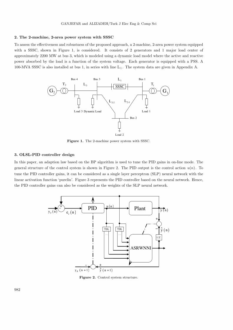
3. OLSL-PID controller design
In this paper, an adaption law based on the BP algorithm is used to tune the PID gains in on-line mode. The
general structure of the control system is shown in Figure 2. The PID output is the control action u(n). To
tune the PID controller gains, it can be considered as a single layer perceptron (SLP) neural network with the
linear activation function ‘purelin’. Figure 3 represents the PID controller based on the neural network. Hence,
the PID controller gains can also be considered as the weights of the SLP neural network.
( )u n
( )y n
+
( )y n−
( )1y n^
^
+( )1dy n +
+
PID
ASRWNNI
Plant( )dy n
+−
( )ce n
−
Figure 2. Control system structure.
982

GANJEFAR and ALIZADEH/Turk J Elec Eng & Comp Sci
∑
pK
iK
dK
PID
U
Activation Function
( )Purelin
Figure 3. The PID controller based on the neural network.
These gains can therefore be updated on-line using the BP algorithm. To select the optimal control
signal, the following cost function can be considered:
Jc (n) =1
2[y (n)− yd (n)]
2=
1
2e2c (n) , (1)
where y(n) is the plant output and yd(n) is the desired plant output, both at time step n . To minimize the
cost function in Eq. (1), the PID controller gains are adjusted on-line using the GD method. The GD method
may be defined as:
W ic (n+ 1) =W i
c (n) + ηic
(− ∂Jc(n)
∂W ic (n)
), (2)
where for Wc =[Kp,Ki,Kd ] and ηc =[ηKp , ηKi , ηKd ], W ic and ηic , respectively, represent an arbitrary gain
and the corresponding learning rate in the PID controller. The partial derivative of the cost function in Eq. (1)
with respect to W ic is:
∂Jc (n)
∂W ic (n)
=
[ec (n)
∂y (n)
∂u (n)
]∂u (n)
∂W ic (n)
. (3)
The components of the weighting vector are also as follows:
∂u (n)
∂Kp= ec, (4)
∂u (n)
∂Ki=
∫ tcurrent
0
ec.dt, (5)
∂u (n)
∂Kd=
d
dtec, (6)
where ∂y(n)/∂u(n) in Eq. (3) is the plant Jacobian in each time step n . Regarding what has been mentioned
so far, the ASRWNNI is used to evaluate the Jacobian on-line. Adjustment of the cycle of the OLSL-PID for
each time step n is given in Appendix B.
4. The ASRWNNI
As mentioned before, the Jacobian of the plant is needed during the adaption process. In this section, the
SRWNN is adapted to design an adaptive plant identifier. This identifier can then be used to evaluate the
Jacobian on-line, based on the indirect adaptive control theory.
983

GANJEFAR and ALIZADEH/Turk J Elec Eng & Comp Sci
4.1. The SRWNN structure
The detailed structure of the SRWNN, consisting of 4 layers with Ni inputs, 1 output, and Ni × Nw mother
wavelets, is shown in Figure 4 [40]. Layer 1 is an input layer. Layer 2 is a mother wavelet layer. Each node
of this layer has a mother wavelet, with the first derivative of a Gaussian function φ(x) = x× exp(–0.5 ×x2)as a mother wavelet function, and a self-feedback loop. Each wavelet (wavelon) φij is derived from its mother
wavelet φ as follows:
Layer 4
Layer 3
Layer 2
Layer 1
y
1xiNξ
1
11Ζ θ− 1
,ω ιΝ ΝΖ θ−11ϕ ,1 ιΝϕ 2, ιΝϕ ,Ν Νω ι
ϕ21ϕ ,1Νω
ϕ
∏ ∏∏1ψ 2ψωΝ
ψ
1w
∑
2w wwN
Figure 4. The SRWNN structure.
ϕij (zij) = ϕ (zij) , ∀zij = ((uij − tij) /dij) , (7)
where tij and dij are the wavelet translation factor and the dilation factor, respectively. The subscript ij
indicates the j th input term of the ith wavelet. Moreover:
uij (n) = xj (n) + ϕij (n− 1) θij ,
where θij shows the weight of the self-feedback loop. Layer 3 is a product layer. The nodes in this layer are
given as follows:
ψi =
Ni∏j=1
ϕ (zij) =
Ni∏j=1
[(zij) exp
(−1
2z2ij
)]. (8)
The network output is finally calculated as:
y (n) =
Nw∑i=1
wiψi, (9)
where wi is the connection weight between the product nodes and the output nodes.
984

GANJEFAR and ALIZADEH/Turk J Elec Eng & Comp Sci
4.2. Application of the SRWNN for the plant identification
The ASRWNNI, based on the series-parallel method [41], can be represented as:
xI = [y (n) , y (n− 1) , ..., y (n− p) , u (n) , u (n− 1) , ..., u (n− q)], (10)
y (n+ 1) = fI (xI) , (11)
where y(n+ 1) is the predicted speed deviation at time step n+ 1 and xI is the input of the ASRWNNI.
Moreover, p and q indicate the number of past output and past input state variables, respectively. Here, both
p and q are chosen to be 1. Our goal is to minimize the following quadratic cost function in both on-line and
off-line modes:
JI (n) =1
2(y (n)− y (n))
2=
1
2eI (n)
2. (12)
Using the GD method, the weight values of the SRWNN are adjusted as follows:
W iI (n+ 1) =W i
I (n) + ηi(− ∂JI (n)
∂W iI (n)
), (13)
where for WI =[tij , dij , θij , wi ] and ηI =[ηt , ηd , ηθ , ηw ], WI and ηiI , respectively, represent an arbitrary
weight and the corresponding learning rate in the SRWNNI. The partial derivative of the cost function with
respect to W iI is:
∂JI (n)
∂W iI (n)
= eI (n)∂eI (n)
∂W iI (n)
= −eI (n)∂y (n)
∂W iI (n)
.
The components of the weighting vector are as follows:
∂y (n)
∂tij (n)= wiψi
(−1
dij
)(1
zij− zij
), (14)
∂y (n)
∂dij (n)= zij
(∂y (n)
∂tij (n)
), (15)
∂y (n)
∂θij (n)= − (ϕij (n− 1))
(∂y (n)
∂tij (n)
), (16)
∂y (n)
∂wi (n)= ψi. (17)
Hence, this identifier can be used for calculating the system sensitivity in each time step n as:
∂y (n+ 1)
∂u (n)≈ ∂y (n+ 1)
∂xI
∂xI∂u (n)
. (18)
From Eq. (10), ∂xI /∂u(n) can be written as [42]:
∂xI∂u (n)
= [0 0 , ..., 1 f1 (z) , ..., fq (z)]T, (19)
where fi(z) = z−i , and
∂y (n+ 1)
∂xI,j=
Nw∑i=1
wi×ψi
(1
dij
)(1
zij− zij
). (20)
985

GANJEFAR and ALIZADEH/Turk J Elec Eng & Comp Sci
5. Convergence analysis for the ASRWNNI
It is important to find the optimal learning rate in an on-line mode because despite the fact that the convergence
is guaranteed for the small values of the learning rate, it should be noted that the speed is very slow. Moreover,
the algorithm becomes unstable for the big values of the learning rate; thus, in this section, the convergence
analysis of the proposed identifier is presented by several theorems.
Theorem 1. Let ηiI be the learning rate for the weights of the ASRWNNI; let g imax be defined as gimax =
maxn||gi (n) || , where gi(n) = ∂y(n)/ ∂W iI and || . || is the usual Euclidean norm in ℜn ; then the convergence
is guaranteed if ηiI is chosen as:
0 < ηiI < 2/(gimax
)2. (21)
Proof. See Appendix C.
Theorem 2. Let ηwI be the learning rate for the weight wI of the ASRWNNI. Next, the convergence is
guaranteed if the learning rate satisfies 0 < ηwI < 2/N w .
Proof: See Appendix D.
Theorem 3. Let ηtI , ηdI , and ηθI be the learning rates of the translation, dilation, and self-feedback weights
for the ASRWNNI in the indirect adaptive control structure, respectively. The convergence is guaranteed if the
learning rates satisfy:
0 < ηtI <2
NwNi
[|d|min
|w|max × 2 exp (−0.5)
]2, (22)
0 < ηdI <2
NwNi
[|d|min
|w|max × 2 exp (0.5)
]2, (23)
0 < ηθI <2
NwNi
[|d|min
|w|max × 2 exp (−0.5)
]2. (24)
Proof: See Appendix E.
Remark 1. The maximum learning rate that guarantees the most rapid or optimal convergence corresponds
to [33]:
ηw,maxI =
1
Nw, (25)
ηt,maxI =ηθ,max
I =1
NwNi
[|d|min
|w|max × 2 exp (−0.5)
]2, (26)
ηd,maxI =
1
NwNi
[|d|min
|w|max × 2 exp (0.5)
]2. (27)
It should be noted that in all of the studies in this section, the assumption was that the network’s data
are not normalized. Obviously, the obtained equations should be generalized for when the data have been
normalized.
986

GANJEFAR and ALIZADEH/Turk J Elec Eng & Comp Sci
6. Simulation results and discussion
6.1. Preliminary
In this section, simulation studies are conducted for the example power system subjected to both severe and
small disturbances under different operating conditions. The results are presented in 3 cases and 2 operating
points, as shown in the Table.
Table. Operating conditions.
Cases P1 Q1 P2 Q2 Pdynamicload Qdynamicload
OP1 0.7619 –0.0478 0.7509 0.0513 1.5711 0.0718OP2 0.8589 0.0539 1 0.0750 1.9981 0.1076
These cases are also as follows: first without a controller (NC), second with the fixed-gain PI controller,
and third with the OLSL-PID controller. The PI controller is initially tuned, carefully. Afterwards, its
parameters are kept unchanged for all of the performed tests. The PI gains are given in Appendix F.
The single-line block diagram of the SSSC control system with an OLSL-PID controller is shown in
Figure 5.
qREFV
qV
12 0dω −Δ =
PWM
Modulator
12ω∧Δ
12ω∆
PID Controller
− +
ASRWNNI
TDLTDL
U max
min
β −+
α 1/β1/
dI
12 0dω −∀ Δ =( )12 12 dce ω ω
−= Δ −Δ
Injected Voltage
Regulator
DC Voltage
Regulator
DC REFV −
DCV
θ
VSC Pulses
PID Controller
d-ConvV
q-ConvV
Figure 5. Single-line diagram of the SSSC control system with an OLSL-PID controller.
Our simulation studies show that a 2-order identifier is accurate enough to calculate the Jacobian of the
example power system on-line, meaning that the ASRWNNI has 4, 32, 8, and 1 neurons at the input, mother
wavelet, wavelet, and output layers, respectively. It should be noted that the input and output signals of the
ASRWNNI are scaled to the range of [–1, 1] using parameters α and β (here α = 0.15 and β = 0.007).
First, the ASRWNNI is trained off-line over a wide range of operating conditions and disturbances.
During this phase, the input and the desired output of the ASRWNNI are [∆ω(n − 1), ∆ω(n − 2), u(n-1),
u(n -2)] and ∆ω(n), respectively. Later on, the ASRWNNI is placed in the system, as shown in Figures 2 and 5.
During this phase, the input and desired output of the ASRWNNI are [∆ω(n), ∆ω(n−1), u(n), u(n−1)] and
987

GANJEFAR and ALIZADEH/Turk J Elec Eng & Comp Sci
∆ω(n + 1), respectively. Furthermore, the on-line training of the ASRWNNI is performed in every sampling
period using the BP algorithm with ALRs.
The difference in the speed deviations of the generators in the 2 areas (ω1 − ω2) is chosen as the control
input of the PID in this paper. All of the PID gains are initially set to those of the conventional PI controller.
Eventually, the PID controller is placed in the system and its parameters are updated in on-line mode using
the BP algorithm, based on the information provided by the ASRWNNI.
For the adaptive controller implementation, a sampling rate is also needed. Such factors as the ability
of controller, the ability of controller’s adaption law, the complexity of the plant, and so on have effects on
the selection of the sampling rate. Hence, the sampling rate selection problem does not follow any systematic
approaches; it is based on trial and error. In this paper, based on our trial-and-error studies, a sampling rate
of 40 Hz is selected.
6.2. Nonlinear time-domain simulation
6.2.1. The results at OP1
To assess the effectiveness of the proposed controller under transient conditions, the 3-phase fault of a 10-cycle
duration at bus 1 is selected as the first disturbance. The results include the system responses and identifier
performance, as presented in Figure 6. It is evident from the results that the OLSL-PID provides better damping
performance than the PI controller, significantly improving the transient stability performance of the example
power system thanks to intelligent variations of its gains, while the ASRWNNI provides a promising tracking
performance.
0 1 2 3 4 5 6 7 8 9 10
-6
-4
-2
0
2
4
6
x 10 -3
NCPI ControllerOLSL-PID Controller
0 1 2 3 4 5 6 7 8 9 10-6
-4
-2
0
2
4
6
8x 10 -3
AS
RW
NN
I P
erfo
rman
ce
ASRWNNIPLANT
0 1 2 3 4 5 6 7 8 9 102550
2551
2552
2553
0 1 2 3 4 5 6 7 8 9 101
2
3
4
5
0 1 2 3 4 5 6 7 8 9 10
0.2
0.4
0.6
time, s
η, d
,max
η, θ
,max
η,
= t
,max
η, w
,max
ω1,ω
2pu
0 1 2 3 4 5 6 7 8 9 100
50
100
150
Kp V
aria
tions
0 1 2 3 4 5 6 7 8 9 10
4
5
6
Ki V
aria
tions
0 1 2 3 4 5 6 7 8 9 10-0.2
0
0.2
0.4
time, s
Kd
Var
iati
ons
Figure 6. System responses to a 3-phase to ground fault at bus 1 in OP1 .
988

GANJEFAR and ALIZADEH/Turk J Elec Eng & Comp Sci
The second disturbance is a 10% step decrease in the terminal voltage reference of G1 at time 0.5 s.
The system returns to its original condition at time 5 s. Figure 7 shows the system responses and identifier
performance.
0 1 2 3 4 5 6 7 8 9 10-6
-4
-2
0
2
4
6x 10 -5
NCPI ControllerOLSL-PID Controller
0 1 2 3 4 5 6 7 8 9 1020406080
100120
Kp V
aria
tion
s
0 1 2 3 4 5 6 7 8 9 10
4
5
6
Ki V
aria
tio
ns
0 1 2 3 4 5 6 7 8 9 10
0
0.2
0.4
0.6
time, s
Kd
Var
iati
on
s
0 1 2 3 4 5 6 7 8 9 102550
2551
2552
2553
η, w
,max
η, d
,max
η, t
,max
=η, θ
,max
0 1 2 3 4 5 6 7 8 9 10
1.9971.9981.999
2
0 1 2 3 4 5 6 7 8 9 100.2702
0.2704
0.2706
time, s
0 1 2 3 4 5 6 7 8 9 10-4
-3
-2
-1
0
1
2
3
4
5x 10 -5
AS
RW
NN
I P
erfo
rman
ce
ASRWNNIPLANT
ω1, ω
2,
pu
Figure 7. System responses to a 10% step decrease in the voltage reference of G1 and the return to the original
condition in OP1 .
0 1 2 3 4 5 6 7 8 9 100
0.1
0.2
0.3
0.4
0.5
0.6
0.7
0.8
0.9
x 10-10
time, s
VI(t
) =
0.5
*e
I2(t
)
VI(t
) =
0.5
*e
I2(t
)
0.05 0.1 0.15 0.2 0.25 0.3 0.35 0.4 0.45 0.50
0.1
0.2
0.3
0.4
0.5
0.6
0.7
0.8
0.9
1x 10 -11
time, s
Off
-lin
e E
rror
Figure 8. The identification error to a 10% step decrease in the voltage reference of G1 and the return to the original
condition in OP1 .
989

GANJEFAR and ALIZADEH/Turk J Elec Eng & Comp Sci
It can be observed that the proposed controller provides the best performance, damping out the os-
cillations with a considerable speed. It is also evident that the proposed identifier can track the plant very
satisfactorily thanks to its self-recurrent local structure and, likewise, its stable training algorithm. The intel-
ligent changes in the learning rates are another interesting part of the results. The identification error is also
provided in Figure 8. From the Lyapunov stability theorem, VI(t) is expected to have a negative gradient at all
times; however, due to the continual control effort, this is practically impossible. In Figure 8 it can be observed
that, in the beginning stages of the identification process, the gradient of VI(t) is negative. This is because the
controller output is absent in these stages, and the identifier learning rates are successfully founded by the ALR
algorithm and the identifier makes efforts to minimize the off-line training error. Following the fault striking,
the PID gains are suddenly changed and the raised control signal is applied to both the plant and the identifier.
Sudden changes of the control signal cause the identifier performance to be degraded, and, consequently, the
VI(t) cannot maintain its negative gradient. However, it should be noted that during the control process, the
ALR helps the identifier to track the plant with the minimum possible error. At the end of the control process,
the control signal is reduced again, and the VI(t) is effectively decreased with a negative gradient.
6.2.2. The results at OP2
To test the robustness of the proposed controller, the system loading condition is changed to OP2 . A 3-phase
fault of a 10-cycle duration at bus 1 is selected as the first proposed disturbance. The results, including the
system responses and identifier performance, are presented in Figure 9. The second disturbance is a 10% step
decrease in the terminal voltage reference of G2 at time 0.5 s. The system returns to its original condition at
time 5 s. Figure 10 shows the system responses and the identifier performance.
0 1 2 3 4 5 6 7 8 9 10-5
-4
-3
-2
-1
0
1
2
3
4
5x 10
-3
NCPI ControllerOLSL-PID Controller
0 1 2 3 4 5 6 7 8 9 10-3
-2
-1
0
1
2
3
4
5x 10
-3
AS
RW
NN
I P
erfo
rman
ce
ASRWNNIPLANT
0 1 2 3 4 5 6 7 8 9 102550
2552
2554
0 1 2 3 4 5 6 7 8 9 102
3
4
0 1 2 3 4 5 6 7 8 9 100.2
0.4
0.6
time, s
0 1 2 3 4 5 6 7 8 9 100
100
Kp V
aria
tions
0 1 2 3 4 5 6 7 8 9 10
4
6
8
Ki V
aria
tions
0 1 2 3 4 5 6 7 8 9 10-1
0
1
2
time, s
Kd
Var
iati
ons
η, w
,max
η, d
,max
ω1,ω
2p
u
η, θ
,max
η,
= t
,max
Figure 9. System responses to a 3-phase to ground fault at bus 1 in OP2 .
990

GANJEFAR and ALIZADEH/Turk J Elec Eng & Comp Sci
Again, it is clear from all of the results presented in this section that the proposed approach provides
the best control performance for different types of disturbances at different operating points of the system,
significantly improving the stability performance of the system despite a considerable change in the system’s
operating point. It can therefore be concluded that the OLSL-PID controller and the ASRWNNI have acceptable
robustness to the operating condition.
0 1 2 3 4 5 6 7 8 9 10-8
-6
-4
-2
0
2
4
6
8x 10
-5
NCPI ControllerOLSL-PID Controller
0 1 2 3 4 5 6 7 8 9 100
50
100
Kp
Vari
ati
ons
0 1 2 3 4 5 6 7 8 9 10
4
5
6
Ki V
ari
ati
ons
0 1 2 3 4 5 6 7 8 9 10-0.2
00.20.40.6
time, s
Kd
Vari
ati
ons
0 1 2 3 4 5 6 7 8 9 102550
2552
2554
0 1 2 3 4 5 6 7 8 9 10
1.996
1.998
2
0 1 2 3 4 5 6 7 8 9 10
0.27
0.2705
time, s
0 1 2 3 4 5 6 7 8 9 10-8
-6
-4
-2
0
2
4
6x 10
-5
AS
RW
NN
I P
erf
orm
ance
ASRWNNIPLANT
η, θ
,max
η,
= t
,max
η, d
,max
η, w
,max
ω1,ω
2pu
Figure 10. System responses to a 10 % step decrease in the voltage reference of G2 and the return to the original
condition in OP2 .
The identification error to a 10% step decrease in the voltage reference of G2 and the return to the
original condition are provided in Figure 11. Here again, it can be observed that VI(t) has a negative gradient
in the beginning stages of the identification process and the off-line training error is minimized. However,
following the fault striking, due to the sudden changes of the PID gains, the identifier performance is degraded,
and consequently the VI(t) cannot maintain its negative gradient. At the end of the control process, the VI(t)
is effectively decreased with a negative gradient.
6.3. Extension to 4-machine, 2-area power system
6.3.1. The 4-machine, 2-area power system with SSSC
A 4-machine, 2-area study system installed with a SSSC, shown in Figure 12, is considered. Each area consists
of 2 generator units. The rating of each generator is 900 MVA and 20 kV. Each of the units is connected through
991

GANJEFAR and ALIZADEH/Turk J Elec Eng & Comp Sci
transformers to the 230 kV transmission line. There is a power transfer of 413 MW from area 1 to area 2. Each
generator is equipped with a PSS. The detailed data are given in [43].
0 1 2 3 4 5 6 7 8 9 100
0.2
0.4
0.6
0.8
1
1.2
1.4
1.6
1.8
x 10 -10
time, s
VI (
t) =
0.5
*e
I2(t
)
0.05 0.1 0.15 0.2 0.25 0.3 0.35 0.40
1
2
3
4
5
6
7
x 10 -12
time, s
VI (
t)=
0.5
*e
I 2(t
)
Off
-lin
e E
rror
Figure 11. The identification error to a 10% step decrease in the voltage reference of G2 and return to the original
condition in OP2 .
Area2Area1
2
C7 C9L9L7
987
651
25 km 10 km
110 km 110 km
220 km
4
310 1125 km10 km G3
G4
SSSC
B_SSSC
G2
G1
Line 1
Line 2
Figure 12. Multimachine power system with a SSSC.
6.3.2. Parameter settings
All of the parameter settings, network structures, and training processes are the same as those of the previous
system, the 2-machine, 2-area system. The difference in the speed deviations of generators G1 and G3 is
selected as the input signal of the proposed controller with the aim of damping the interarea oscillations.
Here again, all of the PID gains are initially set to those of the conventional PI controller. The ASRWNNI
is also trained off-line before placing it into the system. All of the input and output signals of the ASRWNNI
are scaled to the range of [–1, 1] using parameters α and β (here α = 0.15 and β = 0.006).
992

GANJEFAR and ALIZADEH/Turk J Elec Eng & Comp Sci
6.3.3. Nonlinear time-domain simulation
The system responses to a 3-phase to ground fault of an 8-cycle duration at bus 8 are shown in Figure 13.
Figure 14 shows the system responses to a 3-phase to ground fault of an 8-cycle duration at bus 9. The results
for a 2-phase to ground fault of an 8-cycle duration at bus 7 are also presented in Figure 15, while Figure 16
shows the system responses to an 8-cycle outage of line 1.
From all of the results presented in this subsection, it can be observed that the proposed controller provides
better performance for interarea oscillations damping in comparison to the PI controller, significantly improving
the transient stability performance of the system subjected to a wide ranges of disturbances. Acceptable
performance of the ASRWNNI for different types of faults can also be deduced from the results.
0 1 2 3 4 5 6 7 8 9 10-10
-8
-6
-4
-2
0
2
4
6
8
x 10-4
NCPI ControllerOLSL-PID Controller
0 1 2 3 4 5 6 7 8 9 1020
40
6080
100
Kp
Vari
ati
ons
0 1 2 3 4 5 6 7 8 9 103.9
4
4.1
4.2
Ki V
ari
ati
ons
0 1 2 3 4 5 6 7 8 9 10
0
0.5
1
time, s
Kd
Vari
ati
on
s
0 1 2 3 4 5 6 7 8 9 103471
3472
3473
3474
0 1 2 3 4 5 6 7 8 9 10
2.522.542.562.58
2.62.62
0 1 2 3 4 5 6 7 8 9 100.34
0.345
0.35
time, s
0 1 2 3 4 5 6 7 8 9 10-6
-4
-2
0
2
4
6
8
x 10-4
AS
RW
NN
I P
erf
orm
an
ce
ASRWNNIPLANT
η, θ
,max
η,
= t
,max
η, d
,max
η, w
,max
ω1,ω
3pu
Figure 13. System responses to a 3-phase to ground fault at bus 8.
993

GANJEFAR and ALIZADEH/Turk J Elec Eng & Comp Sci
0 1 2 3 4 5 6 7 8 9 10-5
-4
-3
-2
-1
0
1
2
3
4
5x 10
-3
NCPI ControllerOLSL-PID Controller
0 1 2 3 4 5 6 7 8 9 10
3040506070
Kp
Vari
ati
on
s
0 1 2 3 4 5 6 7 8 9 10
4
4.1
4.2
Ki V
ari
ati
on
s
0 1 2 3 4 5 6 7 8 9 10
0
0.5
1
time, s
Kd
Vari
ati
on
s
0 1 2 3 4 5 6 7 8 9 103471
3472
3473
3474
0 1 2 3 4 5 6 7 8 9 102.5
2.6
2.7
2.8
2.9
0 1 2 3 4 5 6 7 8 9 10
0.34
0.36
0.38
time, s
0 1 2 3 4 5 6 7 8 9 10-4
-3
-2
-1
0
1
2
3x 10
-3
AS
RW
NN
I P
erf
orm
ance
ASRWNNIPLANT
η, w
,max
η, d
,max
η, θ
,max
η,
= t
,max
ω1,ω
2pu
Figure 14. System responses to a 3-phase to ground fault at bus 9.
0 1 2 3 4 5 6 7 8 9 10-5
-4
-3
-2
-1
0
1
2
3
4
5x 10
-3
NCPI ControllerOLSL-PID Controller
0 1 2 3 4 5 6 7 8 9 10
3040506070
Kp
Vari
ati
on
s
0 1 2 3 4 5 6 7 8 9 10
4
4.1
4.2
Ki V
ari
ati
on
s
0 1 2 3 4 5 6 7 8 9 10
0
0.5
1
time, s
Kd
Vari
ati
on
s
0 1 2 3 4 5 6 7 8 9 103471
3472
3473
3474
0 1 2 3 4 5 6 7 8 9 102.5
2.6
2.7
2.8
2.9
0 1 2 3 4 5 6 7 8 9 100.34
0.36
0.38
time, s
0 1 2 3 4 5 6 7 8 9 10-4
-3
-2
-1
0
1
2
3x 10
-3
AS
RW
NN
I P
erf
orm
an
ce
ASRWNNIPLANT
η, w
,max
η, d
,max
η, θ
,max
η,
= t
,max
ω1,ω
3p
u
Figure 15. System responses to a 2-phase to ground fault at bus 7.
994

GANJEFAR and ALIZADEH/Turk J Elec Eng & Comp Sci
0 1 2 3 4 5 6 7 8 9 10-1
-0.5
0
0.5
1
1.5x 10⁻³
NCPI ControllerOLSL-PID Controller
0 1 2 3 4 5 6 7 8 9 10
50
100
150
Kp
Var
iati
on
s
0 1 2 3 4 5 6 7 8 9 103.8
4
4.2
Ki V
aria
tio
ns
0 1 2 3 4 5 6 7 8 9 10
0
1
2
3
time, s
Kd
Var
iati
on
s
0 1 2 3 4 5 6 7 8 9 103471
3472
3473
3474
0 1 2 3 4 5 6 7 8 9 102.522.542.562.582.6
2.62
0 1 2 3 4 5 6 7 8 9 100.34
0.345
0.35
time, s
0 1 2 3 4 5 6 7 8 9 10-6
-4
-2
0
2
4
6
8
10
12
14x 10-4
AS
RW
NN
I P
erfo
rman
ce
ASRWNNIPLANT
η, w
,max
η, d
,max
η, θ
,max
η,
= t
,max
ω1,ω
2pu
Figure 16. System responses to a 3-phase to 8-cycle outage of line 1.
7. Conclusions
In this article, to overcome the problems of the fixed-gain PI controller of FACTS devices, an OLSL-PID
controller was developed for power system stability enhancement. The PID controller parameters were updated
based on the information provided by the ASRWNNI, which is a powerful, fast-acting identifier thanks to its
local nature, self-recurrent structure, and stable training algorithm with ALRs based on the discrete Lyapunov
stability theorem. Following the off-line training of the ASRWNNI, it was placed in the final configuration, and
its on-line training was performed in each sampling period. The initial gains of the OLSL-PID were also set
to those of a conventional PI controller, and an adapting ability was then added to it by a BP-based on-line
updating algorithm. Finally, the proposed control scheme was tested in a 2-machine, 2-area power system
under different operating conditions and disturbances. The simulation showed the effectiveness and robustness
of the proposed approach, and thus was promising. The design problem was finally extended to a 4-machine,
2-area benchmark power system in order to damp the interarea modes of the oscillations. The results showed
that the proposed controller provides better performance for interarea oscillation damping in comparison to
the PI controller and they also revealed that because of the high adaptability, the local behavior, and the high
flexibility of both the controller and the identifier, the OLSL-PID can damp the oscillations in a good manner
and significantly improves the transient stability performance of the system.
995

GANJEFAR and ALIZADEH/Turk J Elec Eng & Comp Sci
Appendix A: System data
Generators: SB1 = 2100 MVA, SB2 = 1400 MVA, H = 3.7 s, VB = 13.8 kV, f = 60 Hz, RS = 2.8544e-3,
Xd = 1.305, X ′d = 0.296, X”d = 0.252, Xq = 0.474, X ′
q = 0.243, X”q = 0.18, Td = 1.01 s, T ′d = 0.053 s,
T”d = 0.1 s.
Loads: Load1 = 250 MW, Load2 = 100 MW, Load3 = 50 MW.
Transformers: SBT1 = 2100 MVA, SBT2 = 400 MVA, 13.8/500 kV, f = 60 Hz, R1 = R2 = 0.002, L1 = 0,
L2 = 0.12, D1 /Yg connection, Rm = 500, Lm = 500.
Transmission lines: 3-Ph, 60 Hz, line lengths: L1 = 280 km, L2 = 300 km, L3 = 50 km, R1 = 0.02546
Ω/km, R0 = 0.3864 Ω/km, L1 = 0.9337e-3 H/km, L0 = 4.1264e-3 H/km, C1 = 12.74e-9 F/km, C0 = 7.751e-9
F/km.
SSSC: Snom = 100 MVA, Vnom = 500 kV, f = 60 Hz, maximum rate of change of reference voltage (Vqref ) =
3 pu/s; converter impedances: R = 0.00533, L = 0.16; DC link nominal voltage: VDC = 40 kV; DC link
equivalent capacitance CDC = 375e-6 F; injected voltage regulator gains: KP = 0.00375, Ki = 0.1875; DC
voltage regulator gains: KP = 0.1e-3, Ki = 20e-3; injected voltage magnitude limit: Vq = ±0.2.
PSSs: PSS1 and PSS2 : Ts = 15e-3, Tw = 1, Kp = 0.25, T1 = 0.06, T2 = 1, T3 = T4 = 0.
Appendix B: Adjusting the cycle.
1. If n = 1, then go to step B, else:
(a) Calculate ∂u(n)/∂W ic(n) using Eqs. (4)–(6),
(b) Update the OLSL-PID gains having the “Data I-a” and ec(n+ 1), from the previous time step,
using Eqs. (2) and (3).
2. Calculate u(n) and apply it to both the plant and the ASRWNNI.
3. Calculate following items using a SRWNNI:
(a) ∆y(n+ 1) using Eq. (11) and then ec(n+ 1) (also save ∆y(n+ 1) to use in the next time step as
∆y(n)),
(b) The system Jacobian ∂∆y(n+ 1)/∂u(n) using Eq. (18) and save it as “Data I-a”,
(c) Calculate ALRs for ASRWNNI using Eqs. (25)–(27) and save them as “Data I-b”,
(d) Calculate ∂∆y(n)/∂W iI (n) using Eqs. (14)–(17) and save them as “Data I-c”.
4. If n = 1, then go to step E, else:
(a) Calculate eI (n) having ∆y(n) from the previous time step and using the current value of the plant
output,
i. Train the ASRWNNI having “Data I-b” and “Data I-c” from the previous time step, using Eq.
(13).
5. Go to (A) for the next time step.
996

GANJEFAR and ALIZADEH/Turk J Elec Eng & Comp Sci
A. Appendix C: The proof of Theorem 1.
A discrete-type Lyapunov function can be given by:
VI (n) =1
2e2 (n) , (C.1)
where e(n) = (y(n)− y(n)) represents the error in the learning process. Then:
∆VI (n) = VI (n+ 1)− VI (n)
=1
2
[e2 (n+ 1)− e2 (n)
] . (C.2)
The error difference can be represented by:
e (n+ 1) = e (n) + ∆e (n)
≈ e (n) +
[∂e (n)
∂W iI
]T∆W i
I
, (C.3)
and also:
∆W iI = ηiI
(−∂JI (n)
∂W iI
)= ηiIe (n)
∂y (n)
∂W iI
. (C.4)
Next, from Eqs. (C.2)–(C.4), ∆VI(n) can be represented as:
∆VI (n) = ∆e (n)
(e (n) +
1
2∆e (n)
)= −λe2 (n) ,
where
λ =1
2ηiI∥∥gi (n)∥∥2 (2− ηiI
∥∥gi (n)∥∥2) . (C.5)
If λ > 0 is satisfied, ∆VI(n) < 0. Thus, the asymptotic convergence of the proposed identifier is
guaranteed. Let ηα = ηiI(gimax)
2 [33], and then:
λ ≥ 1
2ηiI∥∥gi (n)∥∥2 (2− ηα) > 0. (C.6)
From Eq. (C.6), we obtain 0 < λα < 2 and Eq. (21) follows. This completes the proof. 2
B. Appendix D: The proof of Theorem 2.
gw(n) = ∂y(n)/∂w , and then we have:
gw (n) =
Nw∑i=1
ψi.
Since we have ψi ≤ 1 for all i ,
∥gw (n)∥ <√Nw
So we have−→ (gwmax)2= Nw.
Accordingly, from Theorem 1, we obtain 0 < ηwI < 2 / N w . This completes the proof. 2
997

GANJEFAR and ALIZADEH/Turk J Elec Eng & Comp Sci
C. Appendix E: The proof of Theorem 3.
In order to prove Theorem 3, the following lemmas are used [33,40].
Lemma 1. Let f(r) = r. exp(−r2). Then, |f(r)| < 1 ∀r ∈ ℜ .
Lemma 1. Let g(r ) = r2. exp(−r2). Then, | g(r)| < 1 ∀r ∈ ℜ .
(A). gt(n) = ∂y(n)/∂t , and then we have:
gt (n) =
Nw∑i=1
wi
(∂ψi
∂t
)
=
Nw∑i=1
wi
Ni∑j=1
(∂ϕ (zij)
∂zij
∂zij∂t
)<
Nw∑i=1
wi
Ni∑j=1
max(−2α. exp (−0.5− α)× −1
d
),
where α =(z2ij − 1
)/2, and according to Lemma 2 |α. exp (−α)| < 1; then we have:
∥∥gt (n)∥∥ <√Nw
√Ni |w|max
2 exp (−0.5)
|d|min
.
Then: (gtmax
)2= NwNi
[|w|max × 2 exp (−0.5)
|d|min
]2.
Accordingly, from Theorem 1, we obtain Eq. (22).
(B). gd(n) = ∂y(n)/∂d , and then we have:
gd (n) =
Nw∑i=1
wi
(∂ψi
∂d
)
=
Nw∑i=1
wi
Ni∑j=1
(∂ϕ (zij)
∂zij
∂zij∂d
)<
Nw∑i=1
wi
Ni∑j=1
max
(−2α.zij exp
(0.5− α− z2ij
)d
) ,
where α =(1− z2ij
)/2, and so according to Lemmas 1 and 2
∣∣zij exp (−z2ij)∣∣ < 1 and |α. exp (−α)| < 1, and
then we have: ∥∥gd (n)∥∥ <√Nw
√Ni |w|max
2 exp (0.5)
|d|min
.
Then: (gdmax
)2= NwNi
[|w|max × 2 exp (0.5)
|d|min
]2.
Accordingly, from Theorem 1, we obtain Eq. (23).
998

GANJEFAR and ALIZADEH/Turk J Elec Eng & Comp Sci
(C). gθ(n) = ∂y(n)/∂θ , and then we have:
gθ (n) =
Nw∑i=1
wi
(∂ψi
∂θ
)
=
Nw∑i=1
wi
Ni∑j=1
(∂ϕ (zij)
∂zij
∂zij∂θ
)<
Nw∑i=1
wi
Ni∑j=1
max
(−2α. exp (−0.5− α)× ϕij (n− 1)
d
) ,
where α =(z2ij − 1
)/2, and according to Lemma 2 |α. exp (−α)| < 1, and then we have:
∥∥gθ (n)∥∥ <√Nw
√Ni |w|max
2 exp (−0.5)
|d|min
.
Then: (gθmax
)2= NwNi
[|w|max × 2 exp (−0.5)
|d|min
]2.
Accordingly, from Theorem 1, we obtain Eq. (24). This completes the proof. 2
D. Appendix F: PI controller parameters
Table F. PID (PI) optimal gains.
Kp Ki Kd
23.86 3.98 0
References
[1] P.W. Sauer, M.A. Pai, Power System Dynamic and Stability, Hoboken, NJ, Prentice Hall, 1998.
[2] M.R. Banaei, A. Kami, “Interline power flow controller (IPFC) based damping recurrent neural network controllers
for enhancing stability”, Energy Conversion and Management, Vol. 52, pp. 2629–2636, 2011.
[3] A.T. Al-Awami, Y.L. Abdel-Magid, M.A. Abido, “A particle-swarm-based approach of power system stability
enhancement with unified power flow controller”, International Journal of Electrical Power & Energy Systems, Vol.
29, pp. 251–259, 2007.
[4] H. Shayeghi, H.A. Shayanfar, S. Jalilzadeh, A. Safari, “A PSO based unified power flow controller for damping of
power system oscillations”, Energy Conversion and Management, Vol. 50, pp. 2583–2592, 2009.
[5] H. Shayeghi, H.A. Shayanfar, S. Jalilzadeh, A. Safari, “Design of output feedback UPFC controller for damping of
electromechanical oscillations using PSO”, Energy Conversion and Management, Vol. 50, pp. 2554–2561, 2009.
[6] H. Shayeghi, H.A. Shayanfar, S. Jalilzadeh, A. Safari, “Tuning of damping controller for UPFC using quantum
particle swarm optimizer”, Energy Conversion and Management, Vol. 51, pp. 2299–2306, 2010.
[7] M. Vilathgamuwa, X. Zhu, S.S. Choi, “A robust control method to improve the performance of a unified power flow
controller”, Electric Power Systems Research, Vol. 55, pp. 103–111, 2000.
[8] M.R. Banaei, A.R. Kami, “Improvement of dynamical stability using interline power flow controller”, Advances in
Electrical and Computer Engineering, Vol. 10, pp. 42–49, 2010.
999

GANJEFAR and ALIZADEH/Turk J Elec Eng & Comp Sci
[9] S. Panda, “Robust coordinated design of multiple and multi-type damping controller using differential evolution
algorithm”, International Journal of Electrical Power & Energy Systems, Vol. 33, pp. 1018–1030, 2011.
[10] S. Panda, “Multi-objective evolutionary algorithm for SSSC-based controller design”, Electric Power Systems
Research, Vol. 79, pp. 937–944, 2009.
[11] A. Kazemi, M.V. Sohrforouzani, “Power system damping using fuzzy controlled facts devices”, Electrical Power
and Energy Systems, Vol. 28, pp. 349–357, 2006.
[12] N.G. Hingorani, L. Gyugyi, Understanding FACTS Concepts and Technology of Flexible AC Transmission System,
New York, IEEE Press, 2000.
[13] K.J. Astrom, T. Hagglund, C.C. Hang, W.K. Ho, “Automatic tuning and adaptation for PID controllers – a survey”,
Control Engineering Practice, Vol. 1, pp. 699–714, 1993.
[14] P. Cominos, N. Munro, “PID controllers: recent tuning methods and design to specification”, IEE Proceedings -
Control Theory and Applications, Vol. 149, pp. 46–53, 2002.
[15] J.G. Ziegler, N.B. Nichols, “Optimum setting for automatic controllers”, Transactions of the ASME, Vol. 64, pp.
759–765, 1942.
[16] W.K. Ho, C.C. Hang, L.S. Cao, “Tuning of PID controllers based on gain and phase margin specifications”,
Automatica, Vol. 31, pp. 497–502, 1995.
[17] A.J. Isakson, S.F. Graebe, “Analytical PID parameter expressions for higher order systems”, Automatica, Vol. 35,
pp. 1121–1130, 1999.
[18] S. Skogestad, “Simple analytic rules for model reduction and PID controller tuning”, Journal of Process Control,
Vol. 13, pp. 291–309, 2003.
[19] B. Kristiansson, B. Lennartson, “Robust and optimal tuning of PI and PID controllers”, IEE Proceedings - Control
Theory and Applications, Vol. 149, pp. 17–25, 2002.
[20] E. Grassi, K. Tsakalis, S. Dash, S.V. Gaikwad, W. Macarthur, G. Stein, “Integrated system identification and
PID controller tuning by frequency loop-shaping”, IEEE Transactions on Control Systems Technology, Vol. 9, pp.
285–294, 2001.
[21] C. Lin, Q.G. Wang, T.H. Lee, “An improvement on multivariable PID controller design via iterative LMI approach”,
Automatica , Vol. 40, pp. 519–525, 2004.
[22] F. Zheng, Q.G. Wang, T.H. Lee, “On the design of multivariable PID controllers via LMI approach”, Automatica,
Vol. 38, pp. 517–526, 2002.
[23] M.T. Ho, “Synthesis of H1 PID controllers: a parametric approach”, Automatica, Vol. 39, pp. 1069–1075, 2003.
[24] S.J. Ho, L.S. Shu, S.Y. Ho, “Optimizing fuzzy neural networks for tuning PID controllers using an orthogonal
simulated annealing algorithm OSA”, IEEE Transactions on Fuzzy Systems, Vol. 14, pp. 421–434, 2006.
[25] C. Vlachos, D. Williams, J.B. Gomm, “Solution to the Shell standard control problem using genetically tuned PID
controllers”, Control Engineering Practice, Vol. 10, pp. 151–163, 2002.
[26] C.C. Kao, C.W. Chuang, R.F. Fung, “The self-tuning PID control in a slider-crank mechanism system by applying
particle swarm optimization approach”, Mechatronics, Vol. 16, pp. 513–522, 2006.
[27] L.D.S. Coelho, “Tuning of PID controller for an automatic regulator voltage system using chaotic optimization
approach”, Chaos, Solitons & Fractals, Vol. 39, pp. 1504–1514, 2009.
[28] P. Shamsollahi, O.P Malik, “An adaptive power system stabilizer using on-line trained neural networks”, IEEE
Transactions on Energy Conversion, Vol. 12, pp. 382–387, 1997.
[29] P. Shamsollahi, O.P Malik, “Direct neural adaptive control applied to synchronous generator”, IEEE Transactions
on Energy Conversion, Vol. 14, pp. 1341–1346, 1999.
[30] J. He, O.P. Malik, “An adaptive power system stabilizer based on recurrent neural networks”, IEEE Transactions
on Neural Networks, Vol. 12, pp. 413–418, 1997.
1000

GANJEFAR and ALIZADEH/Turk J Elec Eng & Comp Sci
[31] T. Kobayashi, A. Yokoyama, “An adaptive neuro-control system of synchronous generator for power system
stabilization”, IEEE Transactions on Energy Conversion, Vol. 11, pp. 621–630, 1996.
[32] W. Liu, G.K. Venayagamoorthy, D.C. Wunsch 2nd, “Adaptive neural network based power system stabilizer design”,
INNS-IEEE International Joint Conference on Neural Networks, pp. 2970–2975, 2003.
[33] S.J. Yoo, J.B. Park, Y.H. Choi, “Stable predictive control of chaotic systems using self-recurrent wavelet neural
network”, International Journal of Control, Automation, and Systems, Vol. 3, pp. 43–55, 2005.
[34] R.J. Wai, J.M. Chang, “Intelligent control of induction servo motor drive via wavelet neural network”, Electric
Power Systems Research, Vol. 61, pp. 67–76, 2002.
[35] Y. Oussar, I. Rivals, L. Personnaz, G. Dreyfus, “Training wavelet networks for nonlinear dynamic input-output
modeling”, Neurocomputing, Vol. 20, pp. 173–188, 1998.
[36] J. Zhang, G. Walter, Y. Miao, W.N.W. Lee, “Wavelet neural networks for function learning”, IEEE Transactions
on Signal Processing, Vol. 43, pp. 1485–1497, 1995.
[37] Q. Zhang, A. Benveniste, “Wavelet networks”, IEEE Transactions on Neural Networks, Vol. 3, pp. 889–898, 1992.
[38] Y. Oussar, G. Dreyfus, “Initialization by selection for wavelet network training”, Neurocomputing, Vol. 34, pp.
131–143, 2000.
[39] Lekutai G, “Adaptive self-tuning neuro wavelet network controllers”, PhD, Virginia Polytechnic Institute and State
University, Blacksburg, VA, USA, 1997.
[40] S.J. Yoo, J.B. Park, Y.H. Choi, “Indirect adaptive control of nonlinear dynamic systems using self-recurrent wavelet
neural networks via adaptive learning rates”, Information Sciences, Vol. 177, pp. 3074–3098, 2007.
[41] K.S. Narendra, K. Parthasarathy, “Identification and control of dynamic system using neural network”, IEEE
Transactions on Neural Networks, Vol. 1, pp. 4–27, 1990.
[42] K.S. Narendra, K. Parthasarathy, “Gradient methods for the optimization of dynamical systems containing neural
networks”, IEEE Transactions on Neural Networks, Vol. 2, pp. 252–262, 1991.
[43] P. Kundur, Power System Stability and Control, New York, McGraw-Hill, 1993.
1001