On-line calibration monitoring system

based on data-driven model for oil well

sensors ⋆

Andre A. Boechat ∗ Ubirajara F. Moreno ∗

Decio Haramura, Jr. ∗

∗ Automation and Systems Department, Federal University of SantaCatarina, Brazil, (email: {boechat, moreno, deciohjr}@das.ufsc.br)

Abstract: In the oilfield industry, data collected from well sensors plays an important role inperformance and security applications. The quality of the measurements is directly related tothe accuracy of the control actions and the optimisation of the production. On-line calibrationmonitoring systems can determine drifts in the sensors measurements and provide more reliableinformation to the user. In this paper, a robust on-line calibration monitoring system for driftcorrection/detection in well sensors is presented and evaluated for simulated and real datasets. Comparisons with a state-of-art monitoring system is also showed. The results indicate apromising applicability of the calibration monitoring system for the oilfield industry data.

Keywords: Performance monitoring, Sensor failures, Drift, Calibration, Prediction methods,Non-parametric regression, Kalman filters.

1. INTRODUCTION

In many industry sectors, the maintenance strategy isbased on traditional approaches to sensor validation, whichinvolves periodic instrument calibration. Various periodicsensor calibration techniques require the process be shutdown and the instrument taken out of service, loaded andcalibrated. In some cases, the costs to repair a sensor areso high that it is left faulty and its data is just ignored,and wrong decisions could be made because of the lack ofinformation.

In the oilfield industry, permanent downhole sensors andsubsea sensors, for offshore platforms, have a great impor-tance for control actions, production optimisation and wellmonitoring. Due to the harsh environmental conditionsin which these sensors are deployed, their reliability isdegraded throughout the well life. However, as Aggrey andDavies (2007) stated, “replacement of a failed sensor rarelyoccurs in practice even when data is known to be incorrect(or completely missing) due to the cost implication of aworkover”. In addition, Eck et al. (1999) point out aboutpermanent downhole gauges, “once in place, the devicesare not routinely repaired, replaced or recovered”.

For these reasons, less invasive and more efficient main-tenance strategies are desirable. Condition based mainte-nance techniques can lead to optimal maintenance, oncethe steady state performance of instruments are monitoredduring plant operation and physical recalibrations are per-formed only when their performance is degraded.

On-line calibration monitoring consists essentially in esti-mating the correct measurements that the sensors shouldhave read and monitoring continuously the difference be-

⋆ This work was supported by Cenpes/Petrobras.

tween estimate values and values of the sensors. Hardwareredundancy can be much expensive, and it may be notso useful to detect faulty sensors that drift in the same di-rection. Moreover, for downhole gauges, redundant compo-nents occupy valuable, limited space and consume preciouspower. Analytical redundancy by models based on physicalequations can generates accurate results, but it is alwayshard or impossible to obtain in practice. Empirical modelsdeveloped with historical data also rely on relationshipsbetween correlated measurements within a system, butthese relationships are formulated in a implicitly way bytraining the model through analysis of fault-free trainingdata obtained during normal operations.

Success of empirical model applications has already beenreported in industry, like nuclear power industries, as re-ported in Gribok et al. (2000) and Ma and Jiang (2011).There are some works where artificial neural networkswere applied (Aggrey and Davies (2007)), but kernel basedtechniques are among the most used techniques. The maintechniques are based on Auto-Associative Kernel Regres-sion (Hines et al. (2008) and An et al. (2011)),MultivariateState Estimation Technique (Gribok et al. (2000)) andSupport Vector Machine for Regression (Gribok et al.(2000), and Takruri et al. (2008)).

In this paper is presented a robust on-line calibrationmonitoring system for oil and gas well sensors. The systemis composed of an auto-associative empirical model, aKalman filter and a statistical decision module, basedon the main ideas of Hines et al. (2008) and Takruriet al. (2008). It is proposed that the association of theseideas could improve the results of a state-of-art monitoringsystem when applied to oil well sensors. The goals arecorrecting the readings of sensors and detecting driftoccurrences. The system is evaluated for simulated and

Proceedings of the 2012 IFAC Workshop on AutomaticControl in Offshore Oil and Gas Production, NorwegianUniversity of Science and Technology, Trondheim,Norway, May 31 - June 1, 2012

FrAT2.5

Copyright held by the International Federation ofAutomatic Control

269

real data sets, and the results are compared to thosepresented by the state-of-art system.

In Section 2, details of the system architectures are de-scribed; in Section 3, the simulated and real data setsused to evaluate the monitoring systems are described; inSection 4, the evaluation results are shown; and finally, theconclusions are presented in Section 5.

2. MONITORING SYSTEM ARCHITECTURES

In the monitoring systems based on data-driven techniquescorrelated measurements within a system, fault free train-ing data obtained during normal operations, are used todevelop a empirical model. This data-driven model is usedto predict future measurements, which are compared withthe real measurements, generating residuals. Any faults inthe system may cause statistically abnormal changes inthese residuals and could be detected by performing sta-tistical tests. If a sensor is working properly, the residualsnormally has a zero mean and a variance related to theamount of noise in the signal of the sensor.

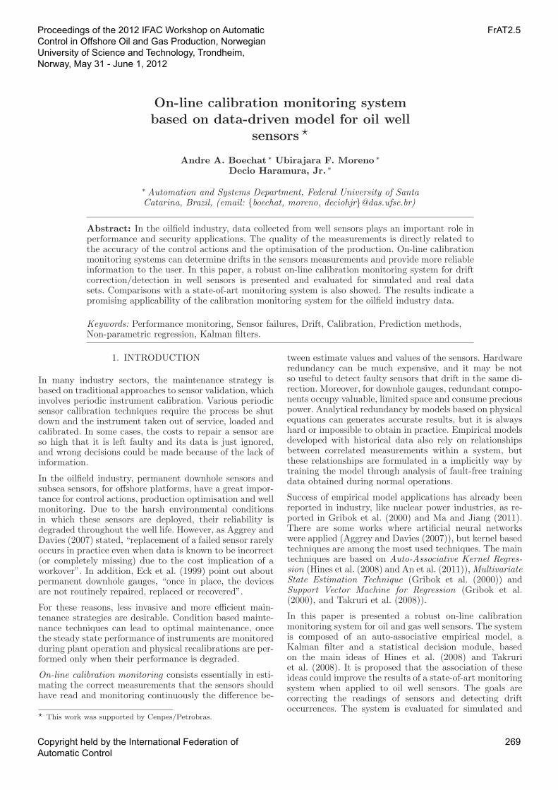
The state-of-art architecture is illustrated in Fig. 1. Inthis paper, this architecture is referenced as AAKR-SPRT,which is composed of two components: a Auto-AssociativeKernel Regression model (AAKR) and a statistical de-cision logic module. The empirical model is developedusing a fault free data set Xn×p, where n is the numberof observations of p different process variables. When anew measurements vector r1×p is available, the predictionof its correct values, x̂1×p, is calculated. The differencebetween the sensors readings r1×p and the predictionsx̂1×p is called residual d1×p. Finally, d1×p is analysed bya statistical module where the sequential probability ratiotest (SPRT) is implemented, indicating a possible driftoccurrence, D ∈ [0, 1].

The architecture of the robust system, AAKR-KF-SPRT,include a Kalman filter (KF) for drift estimation, asin Takruri et al. (2008). The KF is used to track theamplitude of the drift over time, allowing a correction ofthe sensor readings used by the AAKR model. The ideais to reduce the drift effects on the AAKR predictions.

Fig. 1. Process diagrams of the monitoring system archi-tectures: the AAKR-SPRT on left, the AAKR-KF-SPRT on right.

Like the AAKR-SPRT, a AAKR model is developed usinga fault free data set Xn×p. A new measurements vectorr1×p is corrected using a estimation of the drift at the

previous stage d̂k−1

1×p. The corrected measurements x1×p

are inputted into the AAKR model. The estimation of thecorrected measurements, x̂1×p, and r1×p are used by the

KF to calculate a new estimation of the drift, d̂k1×p, which

will be used to correct the next sensor measurements.Then, d̂k

1×p is analysed by the SPRT algorithm, indicatinga possible drift occurrence, D ∈ [0, 1]. The architecture isillustrated in Fig. 1.

The following subsections give more details about eachcomponent of the architectures and some performancemetrics.

2.1 AAKR Model

Auto-Associative Kernel Regression (AAKR) is a typeof similarity based model, a nonparametric modellingtechnique that uses the similarity of a query vector tomemory or exemplar vectors to infer the response of themodel, as described in Hines et al. (2008). The derivationof the AAKR model architecture used in this work isbased on multivariate, inferential kernel regression, thatuses historical, fault free observations to correct drifts inthe current observations. These fault free observations arestored in a matrix Xn×p, where Xi,j is the ith observationof the jth variable, n is the number of observations of the pvariables. A query vector x is a 1× p vector of the sensorsmeasurements, which is the input of the model.

The prediction of the corrected input is calculated as aweighted average of the memory vectors stored in Xn×p,following some basic steps. First, the distance between aquery vector x and each of the memory vectors Xi,j iscalculated. The most common measure is the Euclideandistance. This calculation results in a vector un×1:

u =

u1(X1,x)...

un(Xn,x)

, (1)

ui(Xi,x) =√

(Xi,1 − x1)2 + · · ·+ (Xi,p − xp)2

These distances are converted into similarity measures

wn×1 = [w1 · · · wn]Tby using a kernel function, like the

Gaussian kernel

w =1√2πh2

exp

(

−u2

h2

)

(2)

where h is called kernel bandwidth. Finally, the predictionof the corrected input is calculated by using this similari-ties, or weights, to form a weighted average of the memoryvectors:

x̂j =

n∑

i=1

(wi ·Xi,j)

n∑

i=1

wi

, x̂ =wT Xn∑

i=1

wi

(3)

where x̂ = [x̂1 · · · x̂p] is the prediction vector.

Copyright held by the International Federation ofAutomatic Control

270

It is import to note that the memory vectors must includeall the condition operations that are expected to be in-cluded into the future query vectors. As discussed by Hineset al. (2008), “several circumstances, including equipmentrepair or failure, seasonal variations and system-operatingchanges, can cause a change in operating conditions”. Ifthese operating conditions are not included in the memoryvectors, no confidence can be given to predictions of themodel and the memory matrix must either be appended orreplaced with new data. The distance between the queryvector and the most similar memory vector could indicateif the operating condition is inside of the training region.

In this work, the memory vectors were selected from atraining set by a combination of min-max and vectorordering methods, as described in Hines et al. (2008). Thebandwidth were chosen using grid-search and k-fold cross-validation, as in An et al. (2011). Large bandwidths pro-duce smoother model predictions, as many memory vectorsare used to infer a parameters value. Conversely, smallbandwidths produce rough and/or inconsistent predictionsbecause a limited number, if any, of the memory vectorsare used to infer a parameters value.

2.2 Kalman Filter Model

As illustrated in Fig. 1, the objective of the Kalmanfilter is to estimate or to track the drift embedded in themeasurements. The mathematical model used to estimatethe drift dk

p×1 is

dk = I dk−1 + vk, vk ∼ N (0,V) (4)

where vk is assumed to be Gaussian noise and V is thestate noise covariance. In target tracking, equation (4)is known as the mathematical model of the dynamicsbehaviour of the target. In this work, the sensor drift isthe target, and the objective is to track the amplitude ofthe drift over time. Like Takruri et al. (2008), assumingthe sensor drifts in a smooth, slowly increasing, linearor exponential fashion, the model of equation (4) is areasonable approximation. Another assumption is thatthe drifts are not correlated with each other, despite thecorrelation between the process variables.

The available observations of the drifts, z, is given by

z = r− x̂ (5)

The vector z is not the true values of the drifts, since thetrue values of the process variables are unavailable. So, themeasurement equation is

z = I dk + qk, qk ∼ N (0,Q) (6)

where qk is Gaussian noise and Q is the measurementnoise covariance.

When a reading vector r and the estimation of its correctvalue, x̂, are available, the following steps are executed to

obtain a new estimation of the drifts, d̂k:

(1) prediction, d̂k|k−1 = I d̂k−1

(2) minimum prediction MSE (mean squared error) ma-trix, Mk|k−1 = Mk−1 +V

(3) Kalman gain, Kk = Mk|k−1 (Q+Mk|k−1)−1

(4) correction, d̂k = d̂k|k−1 +K (z− d̂k|k−1)

(5) minimum MSE matrix, Mk = (I−K)Mk|k−1

In Section 4, the Kalman Filter parameters,Q andV, werechosen using trial and error. If Q is set to a high value,the estimated drift takes longer to follow the real drift,whereas if Q is set to a small values, the estimated driftfollows any little difference between the AAKR estimationand the sensor readings. TheV values have a inverse effect:high values yield unstable drift estimates that follow anylittle difference between the AAKR estimation and thesensor readings; for small values, the estimated drift takeslonger to follow the real drift.

2.3 Statistical Decision Logic Module

The statistical decision logic module is responsible forevaluating the residuals and then making a decision aboutthe operating condition of the sensor. In this work, theSPRT algorithm is applied to the residual analysis, de-tecting statistical changes in the residuals between themeasurements and the predict values.

The SPRT is a statistical technique for system anomalydetection (Hines et al. (2008)), which consists of testingtwo possible hypotheses: the system is more likely to bein a normal mode H0 or in a degraded mode H1. For eachnew residual dip of the process variable p (i is the instanttime), the following procedure is executed to accept one ofthe two hypotheses:

(1) calculation of the log-likelihood ratio

Λip = ln

P (dip|H1)

P (dip|H0)(7)

(2) calculation of the cumulative sum of Λp

Sip = Si−1 + Λi

p (8)

(3) application of the stopping rule, a simple thresholdingscheme• lnA < Si

p < lnB, continue monitoring and

calculating Si+1p = Si

p + Λi+1p

• Sip ≤ lnA, H0 is accepted

• Sip ≥ lnB, H1 is accepted and a alarm is emitted

where A and B are the lower and upper bound, andP (dip|H1) is the probability of observing dip given H1

is true. A and B could be defined by the false alarmprobability α and missed alarm probability β as

A =β

1− α, B =

1− β

α(9)

If Sip ≤ lnA, it is determined to belong to the normal mode

H0 of the system and D = 0. Conversely, if Sip ≥ lnB, it

is determined to belong to the degraded mode H1 of thesystem and D = 1, indicating a drift occurrence.

Here the residuals are assumed to be normally distributedwith zero mean and variance of σ2, which is an estimateof the sensor noise. Therefore, the probability distributionfunction for the normal mode of the residuals is given by

P (dip|H0) =1

2πσ2exp

(

−di 2p2σ2

)

(10)

Supposing the degraded mode represented as a mean shiftup (+M) or a mean shift down (−M), where M is the

Copyright held by the International Federation ofAutomatic Control

271

amplitude of the change, the log-likelihood ratio is givenby

Λip =

{

M/σ2(dip −M/2), for a positive changeM/σ2(−dip −M/2), for a negative change

(11)

As suggested in Hines et al. (2008), the optimal M valuecan be determined numerically by applying the SPRT tounfaulted, test data and locating the M value that resultsin a false-alarm probability that is nearest the theoreticalfalse alarm probability α.

2.4 Performance Metrics

As stated in Hines et al. (2008), the performance of auto-associative on-line monitoring systems has traditionallybeen measured in terms of three metrics: accuracy, autosensitivity, and cross sensitivity.

The ability of a model to correctly and accurately predictsensor values is measured by the accuracy, and it is isnormally presented as the MSE between sensor predictionsand the measured sensor values. It is important to notethat this metric compares the unfaulted, or error corrected,predictions with the target, or error free, data. The equa-tion for a single variable is given by

MSE =1

N

N∑

i=1

(x̂i − xi)2 (12)

where N is the number of test observations.

Auto sensitivity (SA) measures the ability of a model tomake correct sensor predictions when the respective sensorvalue is incorrect due to some sort of fault. The autosensitivity for a sensor k is given by

SAk =1

N

N∑

i=1

|x̂driftik − x̂ik|

|xdriftik − xik|

(13)

where x̂drifti is the drifted prediction, x̂i is the unfaulted

prediction, and xdrifti and xi are the drifted and unfaulted

input, respectively.

The effect a faulty sensor input has on other sensorpredictions is measured by the cross sensitivity (SC). Fora unfaulted sensor j and a drifted sensor k, the crosssensitivity is calculated as

SCk =1

N

N∑

i=1

|x̂driftij − x̂ij |

|xdriftik − xik|

(14)

Good monitoring systems have lower MSE, SA and SC

values.

3. DATA SETS FOR SYSTEMS EVALUATION

The two monitoring systems were evaluated using simu-lated and real data sets. Following, major details are givenabout each data set.

3.1 Simulated Data Set

Simulated data were generated by a model developed usingOLGA 1 . The model represent a well operated by gas-lift1 http://www.sptgroup.com/en/Products/olga/Multiphase-Flow-Simulator/

with a 2500 meters deep pipe production. The pressure atthe separator was keep at 1000 kPa and the reservoir wasset to 18000 kPa.

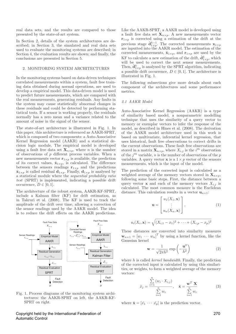
The simulated data were collected during 225 hours ofwell production, while the injected gas flow rate wasset to different values, representing different operatingconditions. The data set is composed of the pressure atthe bottom hole (PTf ), at the top of the production pipe(PTt), at the top of the annular space (PTg) and at theupstream of the injection choke (PTm). The sample ratewas 1 sample per minute. White noise of NSR (noise tosignal ratio) equal to 0.3 was added to the measurements.

The data set was divided into two parts: the first 90 hoursfor AAKR training and the rest of data for test. All thedata set is presented in Fig. 2.

3.2 Real Data Set

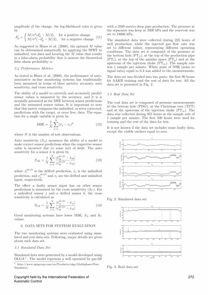
The real data set is composed of pressure measurementsat the bottom hole (PDG), at the Christmas tree (TPT)and at the upstream of the injection choke (PTm). Thedata was collected during 955 hours at the sample rate of1 sample per minute. The first 500 hours were used fortraining and the rest of the data for test.

It is not known if the data set includes some faulty data,except the visible outliers equal to zero.

0 50 100 150 20014

14.5

15

PTf

Pre

ssur

e (M

Pa)

0 50 100 150 2001

2

3

4

PTt

Pre

ssur

e (M

Pa)

0 50 100 150 2001

1.05

1.1

1.15

PTm

Pre

ssur

e (M

Pa)

0 50 100 150 20012

12.5

13

13.5

14

PTg

Pre

ssur

e (M

Pa)

Time (hour)

Fig. 2. Simulated data set.

0 100 200 300 400 500 600 700 800 9000

20

40

60

80

100PDG

Pre

ssur

e (%

)

0 100 200 300 400 500 600 700 800 9000

20

40

60

80

100TPT

Pre

ssur

e (%

)

0 100 200 300 400 500 600 700 800 9000

10

20

30

PTm

Pre

ssur

e (%

)

Time (hour)

Fig. 3. Real data set.

Copyright held by the International Federation ofAutomatic Control

272

4. RESULTS

4.1 Simulated Data

In both architectures, the AAKR model and the SPRTmodule were the same, using the following configurations:an AAKR model with h = 0.2 and 25% × 5400 = 1350memory vectors (almost the most accurate configuration);and a SPRT module with false alarm probability set to5%, missed alarm probability set to 10% andM = 3 (hypo-thetical values) for all process variables. In the AAKR-KF-SPRT architecture, the Kalman Filter covariance matricesQ and V were set to 0.3 and 0.0001, respectively.

In order to evaluate the ability to correct/detect sensorsfaulty data, an artificial linearly increasing sensor driftending at a magnitude of 5σ (five times the standarddeviation of the sensor signal) was introduced in thetesting data set at the time approximately equal to 12hours. The results are presented in Fig. 4, 5, 6 and Table1.

It can be seen in Fig. 4 that the AAKR-KF-SPRT resultsfollow the true values with just a small bias, even at the

0 20 40 60 80 100 120 140

14.3

14.4

14.5

14.6

PTf

Pre

ssure

(MP

a)

True Drifted AKS AS

0 20 40 60 80 100 120 140

1.02

1.04

1.06

1.08

PTm

Pre

ssure

(MP

a)

Time (hour)

Fig. 4. Predictions of PTf and PTm for three driftingsensors, PTf , PTt and PTg, in simulated data set.AKS means AAKR-KF-SPRT and AS means AAKR-SPRT.

0 20 40 60 80 100 120 140−2

0

2

4

PTf

0 20 40 60 80 100 120 140−2

0

2

PTm

Time (hour)

SPRT decision KF residual

Fig. 5. Drift estimates and SPRT decision of PTf and PTm

for the AAKR-KF-SPRT on simulated data set.

0 20 40 60 80 100 120 140−2

0

2

4

PTf

0 20 40 60 80 100 120 140−2

0

2

PTm

Time (hour)

SPRT decision AAKR residual

Fig. 6. Residual and SPRT decision of PTf and PTm forthe AAKR-SPRT on simulated data set.

Table 1. Performance metrics for the systemmonitoring architectures.

AAKR-KF-SPRT AAKR-SPRT

MSE 9.1293× 10−3 2.8491× 10−3

SA 1.9431× 10−5 5.0840× 10−5

SC 8.1022× 10−5 11.8895× 10−5

maximum drift amplitude. The AAKR-SPRT can not gen-erate good predictions for severe drift in its inputs, mainlyfor small bandwidth values. The SA and SC values in Table1 confirm the higher sensitivity of the AAKR-SPRT fordrifting inputs. From the MSE values, the AAKR-SPRTis more accurate for unfaulted data, but the AAKR-KF-SPRT can generate better predictions using faulty data.Larger bandwidths could improve the performance of theAAKR-SPRT, but its predictions tend to be biased, withvalues always near a mean value of the memory vectors.

A comparison of the drift detection performance is showedin the Fig. 5 and 6 2 . The AAKR-SPRT correctly detecteda drift occurrence in PTf at the 56th hours, but itemitted a false alarm about PTm. In addition, the varianceassumed for the sensor noise appear to be in discordancewith the real variance, as it can be seen in the decisionresults of PTf at the time instances around 100 hours, alarge interval between two decisions D = 1. The AKKR-KF-SPRT detected correctly the drift occurrence withoutany false alarms, and its residuals are cleaner, allowingstable drift detection. Since its predictions kept near thetrue values, the residuals reach the limit early.

The better generalisation performance of the AAKR-KF-SPRT allows a greater extension of the useful life sensor,once its predictions are very near the true values even ona severe drift occurrence. However, it has a cost, biasedpredictions even on normal sensor readings. Since the KFcan not discern between bias and drift, incorrect driftpredictions can cause false SPRT alarms.

4.2 Real Data

The following configurations were used for the AAKRmodel and the SPRT module: an AAKR model withh = 0.6 and 5% × 30000 = 1500 memory vectors (almostthe most accurate configuration); and a SPRT modulewith false alarm probability set to 5%, missed alarmprobability set to 10% and M = 3 for all process variables.In the AAKR-KF-SPRT architecture, the Kalman Filtercovariance matrices Q and V was set to 10 and 0.0001,respectively.

Again, an artificial linearly increasing sensor drift endingat a magnitude of 5σ (five times the standard deviation ofthe sensor signal) was introduced in the testing data setat the time approximately equal to 42 hours. The resultsare presented in Fig. 7, 8, 9 and Table 2.

The predictions for two drifting sensors, TPT e PTm,are illustrated in Fig. 7. It can be seen that a similarbehaviour of the monitoring systems when compared toFig. 4. The AAKR-KF-SPRT present better performance

2 The shaded area means the occurrence of many close high and lowvalues. High values indicate D = 1 (degraded mode), whereas lowvalues indicate D = 0 (normal mode).

Copyright held by the International Federation ofAutomatic Control

273

0 50 100 150 200 250 300 350 400 450 5000

20

40

60

80

100

PDG

Pre

ssu

re(%

)

True Drifted AKS AS

0 50 100 150 200 250 300 350 400 450 5000

5

10

15

20

25

PTm

Time (hour)

Pre

ssu

re(%

)

Fig. 7. Predictions of PDG and PTm for two driftingsensors, TPT and PTm in real data set. AKS meansAAKR-KF-SPRT and AS means AAKR-SPRT.

0 50 100 150 200 250 300 350 400 450 500−1

−0.5

0

0.5

1PDG

0 50 100 150 200 250 300 350 400 450 500−2

0

2

4

6

PTm

Time (hour)

SPRT decision KF residual

Fig. 8. Drift estimates and SPRT decision of PDG andPTm for the AAKR-KF-SPRT on real data set.

0 50 100 150 200 250 300 350 400 450 500−20

−15

−10

−5

0

PDG

0 50 100 150 200 250 300 350 400 450 500−10

−5

0

5

PTm

Time (hour)

SPRT decision AAKR residual

Fig. 9. Residual and SPRT decision of PDG and PTm forthe AAKR-SPRT on real data set.

Table 2. Performance metrics for the systemmonitoring architectures on real data set.

AAKR-KF-SPRT AAKR-SPRT

MSE 2.7013 1.4061SA 0.0747 0.6956SC 0.0466 0.1208

for drift correction/detection. The SA and SC values inTable 2 indicate the lower sensitivity for faulty inputspresented by the AAKR-KF-SPRT, whereas the AAKR-SPRT predictions presented some inconsistent peaks, evenfor the PDG data. However, as indicated by the MSEvalues, for unfaulted data, the AAKR-SPRT is moreaccurate, considering the original data as error free. Forthe visible outliers equal to zero, both systems generatedreasonable predictions.

As it can be noted in the Fig. 8 and 9, the residualgenerated by the AAKR-SPRT is affected by outliers in

the test data; its SPRT module gave false alarms for thePDG and missed some alarms for the other sensor. Thedrift estimates of the AAKR-KF-SPRT are much moreclean, resulting in correct SPRT decisions.

Although the performance of the systems have some differ-ences, both systems show promising results for the oilfieldindustry data.

5. CONCLUSION

In this work, a robust on-line calibration monitoring sys-tem for drift correction/detection in oil and gas well sen-sors is presented. The system is based on an empiricalmodel for prediction, a Kalman filter for drift trackingand a statistical decision module for drift detection. Theevaluation for simulated and real data sets demonstratedpromising results for the oilfield industry. With a slight lossof accuracy, the predictions of the corrected readings of thesensors showed to be much less sensitive for drifts than astate-of-art monitoring system. This characteristic allowsa greater extension of the useful life of the sensors, playingan important role on the production optimisation of thewell and planning. For future work, the use of the empiricalmodel uncertainty in the drift detection and improvementsin Kalman filter will be analysed.

ACKNOWLEDGEMENTS

The authors would like to thank Cenpes/Petrobras forprovision of data and financial support.

REFERENCES

Aggrey, G. and Davies, D. (2007). Tracking the state anddiagnosing Down Hole Permanent Sensors in IntelligentWell Completions with Artificial Neural Network. Off-shore Europe.

An, S.H., Heo, G., and Chang, S.H. (2011). Detection ofprocess anomalies using an improved statistical learningframework. Expert Systems with Applications, 38(3),1356–1363.

Eck, J., Ewherido, U., Mohammed, J., and Ogunlowo, R.(1999). Downhole monitoring: the story so far. OilfieldReview, 3(3), 18–29.

Gribok, A., Hines, J.W., and Uhrig, R. (2000). Use ofkernel based techniques for sensor validation in nuclearpower plants. In NPIC&HMIT 2000.

Hines, J.W., Garvey, J., Garvey, D., and Seibert, R.(2008). Technical Review of On-Line Monitoring Tech-niques for Performance Assessment. Volume 3. LimitingCase Studies. Technical report, U.S. Nuclear Regula-tory Commission Office of Nuclear Regulatory Research,Washington, DC.

Ma, J. and Jiang, J. (2011). Applications of fault detec-tion and diagnosis methods in nuclear power plants: Areview. Progress in Nuclear Energy, 53(3), 255–266.

Takruri, M., Rajasegarar, S., and Challa, S. (2008). Onlinedrift correction in wireless sensor networks using spatio-temporal modeling. Information Fusion, 2008 11thInternational Conference on, 1–8.

Copyright held by the International Federation ofAutomatic Control

274