rsta.royalsocietypublishing.org

ResearchCite this article: Tremblay LB, Schmidt GA,Pfirman S, Newton R, DeRepentigny P. 2015 Isice-rafted sediment in a North Pole marinerecord evidence for perennial sea-ice cover?.Phil. Trans. R. Soc. A 373: 20140168.http://dx.doi.org/10.1098/rsta.2014.0168

Accepted: 29 May 2015

One contribution of 6 to a discussion meetingissue ‘Arctic sea ice reduction: the evidence,models and impacts (Part 2)’.

Subject Areas:oceanography, climatology, glaciology

Keywords:Arctic, sea ice, palaeoclimate

Author for correspondence:L. B. Tremblaye-mail: bruno.tremblay@mcgill.ca

Is ice-rafted sediment in aNorth Pole marine recordevidence for perennialsea-ice cover?L. B. Tremblay1,4, G. A. Schmidt2, S. Pfirman3,

R. Newton4 and P. DeRepentigny1

1Department of Atmospheric and Oceanic Sciences, McGillUniversity, 805 Sherbrooke Street West, Montreal, Quebec,Canada H3A OB92NASA Goddard Institute for Space Studies, 2880 Broadway,New York, NY 10025, USA3Barnard College, 3009 Broadway, New York, NY 10027, USA4Lamont-Doherty Earth Observatory of Columbia University,61 route 9W, Palisades, NY 10964, USA

GAS, 0000-0002-2258-0486

Ice-rafted sediments of Eurasian and North Americanorigin are found consistently in the upper part(13 Ma BP to present) of the Arctic Coring Expedition(ACEX) ocean core from the Lomonosov Ridge, nearthe North Pole (≈ 88◦ N). Based on modern sea-icedrift trajectories and speeds, this has been takenas evidence of the presence of a perennial sea-icecover in the Arctic Ocean from the middle Mioceneonwards (Krylov et al. 2008 Paleoceanography 23,PA1S06. (doi:10.1029/2007PA001497); Darby 2008Paleoceanography 23, PA1S07. (doi:10.1029/2007PA001479)). However, other high latitude landand marine records indicate a long-term trendtowards cooling broken by periods of extensivewarming suggestive of a seasonally ice-free Arcticbetween the Miocene and the present (Polyak et al.2010 Quaternary Science Reviews 29, 1757–1778.(doi:10.1016/j.quascirev.2010.02.010)). We use acoupled sea-ice slab-ocean model including sedimenttransport tracers to map the spatial distribution of ice-rafted deposits in the Arctic Ocean. We use 6 hourlywind forcing and surface heat fluxes for two differentclimates: one with a perennial sea-ice cover similarto that of the present day and one with seasonallyice-free conditions, similar to that simulated infuture projections. Model results confirm that in the

2015 The Author(s) Published by the Royal Society. All rights reserved.

on July 17, 2018http://rsta.royalsocietypublishing.org/Downloaded from

2

rsta.royalsocietypublishing.orgPhil.Trans.R.Soc.A373:20140168

.........................................................

present-day climate, sea ice takes more than 1 year to transport sediment from all its peripheralseas to the North Pole. However, in a warmer climate, sea-ice speeds are significantly faster(for the same wind forcing) and can deposit sediments of Laptev, East Siberian and perhapsalso Beaufort Sea origin at the North Pole. This is primarily because of the fact that sea-iceinteractions are much weaker with a thinner ice cover and there is less resistance to drift. Weconclude that the presence of ice-rafted sediment of Eurasian and North American origin atthe North Pole does not imply a perennial sea-ice cover in the Arctic Ocean, reconciling theACEX ocean core data with other land and marine records.

1. IntroductionThe impact of seasonally ice-free conditions in the Arctic, as predicted for the coming century[1–3], can be usefully constrained by examining periods in the Earth’s history when this haspreviously occurred. However, direct evidence of seasonal sea-ice minima is sparse and soinferences need to be made from indicative proxy information which can be derived from manydifferent terrestrial, lacustrine, cryospheric and oceanic archives. Discrepancies do, however, existacross inferences from different archives, and these need to be resolved if we are to make progresson assessing the impacts.

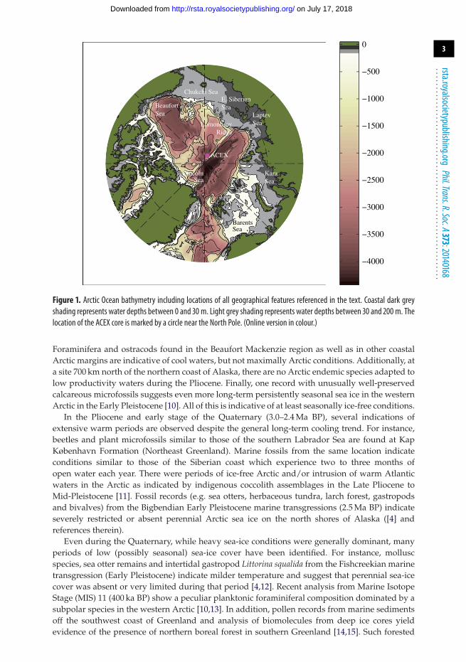
Over the history of the Cenozoic, the first appearance of sea-ice diatoms and sand-sizeice-rafted debris (IRD) in marine sediments suggests an onset of Arctic sea ice ca 47 Myr BP[4–7]. In cores retrieved by the Arctic Coring Expedition (ACEX, in 2004) from the LomonosovRidge near the North Pole (≈ 88◦N), the onset of continuous perennial sea-ice cover in theArctic Ocean is inferred from the rapid change in provenance in the Mid-Miocene (ca 13 MaBP, 156.5 m composite depth or mcd) from clinopyroxene originating in the western Laptev,Kara and Barents seas to amphibole minerals originating in the eastern Laptev and westernEast Siberian seas [8]—coincident with the opening of the Fram Strait and the modern oceaniccirculation (see figure 1 for location of the main geographical features cited in the text). Similarly,Darby [9] concludes that the abundance of sediments originating from the Canadian ArcticArchipelago (CAA) in the same core since 13 Ma BP is indicative of the presence of a perennialsea-ice cover.

In many places in the Arctic, turbidity currents can transport sediments to the deep basins,confusing the interpretation of the sediment record. However, on the Lomonosov Ridge, sea iceis the main transport agent. The relatively low amount of larger IRD which can be transportedby icebergs is also taken as evidence that rafting of sediment via sea ice is the most importantmechanism for deposition of finer grain sizes to the Arctic submarine ridges [9]. For this reason,Darby interprets changes in the provenance of sediments at the core location as changes in sea-icedrift patterns.

With present-day drift speeds and trajectories, it takes approximately 2–3 years for sedimentof East Siberian and eastern Laptev Sea origin to reach the ACEX core site (and approx. 4–5 yearsfor sediment from the Beaufort Sea). Thus, multi-year ice would be necessary to transport thesesediments, implying that the continual presence of amphibole minerals and minerals of CAAorigin at the ACEX core site is indicative of perennial sea-ice cover. Only 133 samples, however,were analysed in the ACEX core over the period of 14 Ma BP to the present. While the time periodbetween most samples is long enough for a temporary reversal to seasonal ice, Darby [9] arguesthat the probability that this condition is missed in all 133 samples is low.

Land and other marine records, on the other hand, show distinct periods of extensive warmingand presumably seasonally ice-free Arctic conditions since the Mid-Miocene ([4] and referencestherein). For instance, pine, birch, spruce and larch are found in Early- to Mid-Pliocene (5.3–3 Ma BP) in the western CAA. Coincidentally, water temperature as high as 18◦C has beenreported on the Yermak Plateau (north of Svalbard), consistent with the presence of subarcticbivalves on Meighen Island (80◦ N 99◦ W) during the Pliocene climatic optimum (ca 3.2 Ma BP).

on July 17, 2018http://rsta.royalsocietypublishing.org/Downloaded from

3

rsta.royalsocietypublishing.orgPhil.Trans.R.Soc.A373:20140168

.........................................................

−4000

−3500

−3000

−2500

−2000

−1500

−1000

−500

0

Chukchi SeaE. SiberianSeaBeaufort

Sea

LomonosovRidge

LaptevSea

KaraSea

BarentsSea

LincolnSea

ACEX

Figure 1. Arctic Ocean bathymetry including locations of all geographical features referenced in the text. Coastal dark greyshading represents water depths between 0 and 30 m. Light grey shading represents water depths between 30 and 200 m. Thelocation of the ACEX core is marked by a circle near the North Pole. (Online version in colour.)

Foraminifera and ostracods found in the Beaufort Mackenzie region as well as in other coastalArctic margins are indicative of cool waters, but not maximally Arctic conditions. Additionally, ata site 700 km north of the northern coast of Alaska, there are no Arctic endemic species adapted tolow productivity waters during the Pliocene. Finally, one record with unusually well-preservedcalcareous microfossils suggests even more long-term persistently seasonal sea ice in the westernArctic in the Early Pleistocene [10]. All of this is indicative of at least seasonally ice-free conditions.

In the Pliocene and early stage of the Quaternary (3.0–2.4 Ma BP), several indications ofextensive warm periods are observed despite the general long-term cooling trend. For instance,beetles and plant microfossils similar to those of the southern Labrador Sea are found at KapKøbenhavn Formation (Northeast Greenland). Marine fossils from the same location indicateconditions similar to those of the Siberian coast which experience two to three months ofopen water each year. There were periods of ice-free Arctic and/or intrusion of warm Atlanticwaters in the Arctic as indicated by indigenous coccolith assemblages in the Late Pliocene toMid-Pleistocene [11]. Fossil records (e.g. sea otters, herbaceous tundra, larch forest, gastropodsand bivalves) from the Bigbendian Early Pleistocene marine transgressions (2.5 Ma BP) indicateseverely restricted or absent perennial Arctic sea ice on the north shores of Alaska ([4] andreferences therein).

Even during the Quaternary, while heavy sea-ice conditions were generally dominant, manyperiods of low (possibly seasonal) sea-ice cover have been identified. For instance, molluscspecies, sea otter remains and intertidal gastropod Littorina squalida from the Fishcreekian marinetransgression (Early Pleistocene) indicate milder temperature and suggest that perennial sea-icecover was absent or very limited during that period [4,12]. Recent analysis from Marine IsotopeStage (MIS) 11 (400 ka BP) show a peculiar planktonic foraminiferal composition dominated by asubpolar species in the western Arctic [10,13]. In addition, pollen records from marine sedimentsoff the southwest coast of Greenland and analysis of biomolecules from deep ice cores yieldevidence of the presence of northern boreal forest in southern Greenland [14,15]. Such forested

on July 17, 2018http://rsta.royalsocietypublishing.org/Downloaded from

4

rsta.royalsocietypublishing.orgPhil.Trans.R.Soc.A373:20140168

.........................................................

landscape indicates warmer July and winter mean temperatures, higher than 10◦ and −14◦C,respectively, and suggests an almost complete disappearance of the Greenland southern ice domeat some point in the last 500 kyr. Conditions leading to such a land ice configuration in Greenlandwould probably be accompanied by low sea-ice conditions in the Arctic.

During the last interglacial (MIS 5e and a), Miller et al. [16] report a 5◦C warmer winter andthe presence of forest along the Eurasian coast of the Arctic and planktonic foram typical ofsubpolar, seasonally ice-free oceans, lived in the central Arctic and north of Greenland [17–19].Given that this is the location where the thickest ice is present today, most of the Arctic may havebeen seasonally ice-free during those two intervals [4], in line with high insolation and warmtemperatures at high northern latitudes at that time.

Most recently, during the Early Holocene, periods of low, but perhaps not seasonally ice-freeArctic, were likely to have been present [20]. Wave-generated beaches from northeast Greenlandover several hundred kilometres indicate seasonally ice-free Arctic in this region as far north as83◦ N [21–23]. Molluscs dating from 8.6 to 6 ka on the same beaches were also present [4], andthere was a minimum of driftwood flux to North of Greenland [24,25]. Driftwood records fromcoastlines north of Ellesmere Island also indicate the absence of perennial land-fast ice present inthis region [26]. During that period bowhead whale records indicate that the CAA was free of iceat least during some months [27]. However, dinocyst assemblages from a marine core north of theChukchi Sea indicate a continuous sea-ice presence throughout the year over the Holocene [28],though this reconstruction comes with large uncertainties.

Given the obvious discrepancy between the central Arctic IRD record and the wealth of otherproxy evidence, the assumptions underlying the interpretation of the IRD record are worthexamining. Specifically, we explore the patterns of sea-ice sediment deposition in a coupled sea-ice and ocean model in varying climate regimes, including one with seasonally ice-free conditions.If sediment can be transported from the East Siberian/Laptev or Beaufort Sea to the ACEX coresite (see figure 1) within one season in a warmer climate, then that would imply that perennialsea-ice cover is not necessarily required to explain the IRD record. Conversely, if sedimentonly reaches this region when multi-year sea-ice cover is present, the inferences of continuousperennial sea ice would be supported.

2. Sediment transport by sea ice and the Arctic Coring Expedition coreWhile some sediment enters the Arctic Ocean via river run-off, and aerially via wind transport,the main source of sediment transported by sea ice is resuspension of shelf sediment. In shallowdepths, the fine fraction of sediment (fine sand, silt and clay) is resuspended via turbulent mixinginduced by winds, tides and ocean currents, and incorporated into sea ice during freeze-up(suspension freezing) [29–31]. While coarser sediments from coastal regions can also be entrainedinto land-fast sea ice, those sediments are redeposited locally the following summer and are notinvolved in long-range transport during the following summer melt. Sediments entrained into seaice in polynya regions located at the edge of the land-fast ice can drift past the continental shelfand be deposited in the central Arctic and beyond when the sea ice melts. During the cold season,ice accretion occurs at the ice base. During the summer, melt occurs both at the surface and at thebase, but, on average, basal ice accretion during winter exceeds basal melt in the summer. For thisreason, sediments tend to be preserved in the sea ice during subsequent summers and appear to‘migrate’ upwards towards the surface after a few freeze/thaw seasonal cycles [32]. When sea-iceridging occurs, this simple series of events is disrupted and distinct layers of sediments can befound at various depths in the ice.

3. Sea-ice modelWe use a coupled slab-ocean sea-ice dynamic-thermodynamic model of the Arctic Ocean and itsperipheral seas with a spatial resolution of 80 km. Sea-ice motion is determined from a balancebetween the surface wind stress on the top of the ice, the ocean drag below, the internal ice stress

on July 17, 2018http://rsta.royalsocietypublishing.org/Downloaded from

5

rsta.royalsocietypublishing.orgPhil.Trans.R.Soc.A373:20140168

.........................................................

resulting from ice floe interactions, the sea surface tilt and the Coriolis term. In this model, sea iceis assumed to behave as a viscous-plastic material with an elliptical yield curve and normal flowrule [33]. The dynamics of the model are forced with 6 hourly varying geostrophic winds from theNational Center for Environmental Prediction and the National Center for Atmospheric Research(NCEP/NCAR) reanalysis. Conservation of mass is used to calculate the temporal evolution ofthe mean sea-ice thickness via thermodynamic (ice growth and melt) and dynamic (ridging andlead opening) processes. A zero-layer (no thermal inertia) thermodynamic model [34] with twoice thickness categories ([33], mean ice thickness h and fraction of a grid cell covered by ice A)is used to calculate the internal sea-ice temperatures and the thermodynamic source term forsurface melt and basal growth/melt. The mechanical source term on the other hand is simply thedivergence of the sea-ice mass flux. The thermodynamics of the model are forced with monthlymean atmospheric fields from the NCEP/NCAR reanalyses. The key parameters defining thedynamics of sea ice (drag coefficients and ice compressive/shear strength) in this model werechosen to minimize the error between the simulated and observed drifts from the InternationalArctic Buoy Programme ([35], IABP).

The model is coupled to a slab-ocean thermodynamic model that calculates the surface oceantemperature taking into account advection of heat by surface ocean currents, diffusion and surfaceocean-atmosphere heat fluxes. Climatological, spatially varying ocean currents are obtained fromthe steady-state solution of the Navier–Stokes equation in which the advection of momentum isneglected, a two-dimensional non-divergent flow field is assumed and a quadratic drag law isused. We chose this simple coupled ice-ocean model forced with contemporaneous atmosphericfield—as opposed to a fully coupled Global Climate Model (GCM)—because of small biases inthe exact geographical location of the Beaufort Gyre that are present in GCMs participating in theCoupled Model Intercomparison Project Phase 5 (CMIP5) (as they were in CMIP3) [36,37]. Thesebiases can lead to significant differences in pathways and transit times between coastal areaswhere sediment is incorporated into sea ice and the ACEX core location. Furthermore, as we arespecifically interested in the dynamics of the seasonal ice pack, the details of the growth/melt ofthe seasonal ice cover do not impact our conclusions. More details about the model and numericalmethod used to solve the sea-ice momentum equation can be found in [38,39].

We perform two basic experiments, a present-day simulation with perennial sea-ice cover(PERENN), and a warmer simulation with a seasonal sea-ice cover (SEASON). For SEASON,the model is run with the same forcing as PERENN but with increased downwelling longwaveradiation. This is done by increasing the emissivity of the atmosphere by a constant factor tosimulate the impact of an increase in greenhouse gas forcing.

For each of the simulations, the model is run for 40 years (1949–1998) starting from realisticinitial conditions (h and A obtained from a 10 year simulation forced with a random set of 10years selected in the 1949–1998 time period). In the autumn (or winter) of each year, when icefirst forms in a model grid cell with depth smaller than 30 m (see figure 1), a passive tracer isintroduced at the grid centre location, representing sediment entrapped in the ice. For PERENNthe tracer is introduced in October, and in SEASON it is introduced in January, when ice first formsin the peripheral seas of the Arctic. The passive tracer is then advected in a Lagrangian mannerand the x–y coordinates, ice thickness, ice concentration and amount of sediment deposited bysea ice at the tracer location are recorded each day.

In the following, we assume that sediments are at the surface of the ice. As sediments canbe present in the interior of the ice, this constitutes a lower-bound (more conservative) estimateof sediment deposited by sea ice. In a two-category sea-ice model, the implied sea-ice thicknessdistribution is linear and ranges from 0 to 2h metres. Therefore, the amount of newly formedopen water area (δA), for a mean sea-ice thickness melt (δh), is equal to δhA/2h. The amount ofsediment deposited at each time step, in turn, can be calculated as SLδA = SLδhA/2h, where SL isthe sediment load per unit area (e.g. 16 tons km−2, [33,38,40]). The total sediment deposited in amodel grid cell for a specified time period is the sum of the sediment deposited at each time step.In the following, we focus on the sediment deposited by a seasonal ice cover and only sedimentdeposited by sea ice of 1 year of age and younger is considered.

on July 17, 2018http://rsta.royalsocietypublishing.org/Downloaded from

6

rsta.royalsocietypublishing.orgPhil.Trans.R.Soc.A373:20140168

.........................................................

0

0.5

1.0

1.5

2.0

2.5

3.0

0

0.5

1.0

1.5

2.0

2.5

3.0

0

0.5

1.0

1.5

2.0

2.5

3.0

3.5

4.0

4.5

5.0

0

0.5

1.0

1.5

2.0

2.5

3.0

3.5

4.0

4.5

5.0

0E

30E

60

E

90E

120E150E

180E

150W

120W

90 W

60 W30 W

80 N

70 N

0E

30E

60

E

90E

120E150E

180E

150W

120W

90 W

60 W30 W

80 N

70 N

0E

30E

60

E

90E

120E150E

180E

150W

120W

90 W

60 W30 W

80 N

(a) (b)

(c) (d)

70 N

0E

30E

60

E

90E

120E150E

180E

150W

120W

90 W

60 W30 W

80 N

70 N

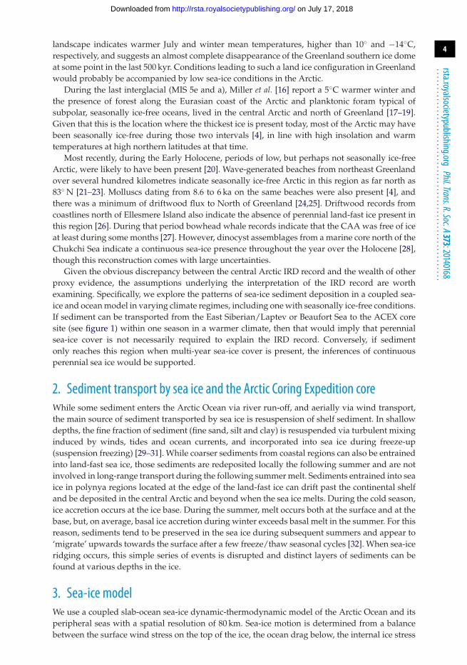
Figure 2. Spatial distribution of March (a–c) and September (b–d) sea-ice thickness (m) for today’s climate with perennialsea-ice cover (a, b; PERENN) and for a warmer climate with only seasonal ice cover (c, d; SEASON). (Online version in colour.)

4. ResultsWe show simulation results for the spatial distribution of sediment transported by sea ice for thetwo different Arctic climates. The simulated sea-ice thickness distribution for PERENN in Marchand September is realistic when compared with observations ([41–43]; figure 2). For SEASON, themaximum sea-ice thickness in the winter decreases from 6 to 3 m and the minimum (September)sea-ice cover is thin (1 m or less) and has retreated far from the Eurasian coastline (figure 2). Itsgeographical location is very similar to that simulated by the Community Climate System Modelfor the year 2040 after a transition to nearly seasonal sea-ice cover described in Holland et al. [3].

For PERENN, sediment of Beaufort, East Siberian and Laptev Sea origin is mainly redepositedon the Yukon, Alaskan and Eurasian shelf with some deposition across the shelf break extendingoutwards towards the central Arctic (figure 3). This supports the suggestion from Krylov et al.[8] that with today’s drift speed and sea-ice circulation pattern, sediment from the Eurasiancoast cannot reach the North Pole ACEX core location in a single season. For SEASON, sedimentdeposition again mainly occurs on the continental shelf break, and also extends far along the pathof the Transpolar drift stream, reaching the ACEX core site and recirculating also in the westernbranch of the Beaufort Gyre (in the case of Eurasian sediment) (figure 4). Note that the transport isfar greater despite the fact that the ice season is much reduced in length (January–June in SEASONas opposed to October–July in PERENN). The main reason for the faster drift speed is the thinnersea-ice cover and the corresponding smaller sea-ice interaction term.

on July 17, 2018http://rsta.royalsocietypublishing.org/Downloaded from

7

rsta.royalsocietypublishing.orgPhil.Trans.R.Soc.A373:20140168

.........................................................

80 N

70 N

0E

30E

60

E

90E

120E150E

180E

150W

120W

90 W

60 W30 W

0E

30E

60

E

90E

120E150E

180E

150W

120W

90 W

60 W30 W0

0.02

0.04

0.06

0.08

0.10

(a) (b)

80 N

70 N

0

0.05

0.10

0.15

0.20

0.25

0.30

0.35

0.40

0.45

88888800000 NNNNNNN

Figure 3. Climatological normalized distribution of sediment deposited by first-year sea ice for present-day climate withperennial sea-ice cover (PERENN) for sediment originating from (a) the East Siberian and Laptev Seas and (b) the BeaufortSea. The thick cross is the location of the North Pole. (Online version in colour.)

80N

70 N

0E

30E

60E

90E

120E150E

180E

150W

120W

90 W

60 W30 W

0E

30E

60E

90E

120E150E

180E

150W

120W

90 W

60 W30 W

0.005

0.010

0.015

0.020

0.025

0.030

0.035

0.040

80 N

70 N

0

0.05

0.10

0.15

0.20

0.25

(b)(a)

880800NNNN0N80NNNN880NN

18

8800

Figure 4. Climatological normalized distribution of sediment deposited by first-year sea ice for a warmer climate with onlyseasonal sea-ice cover (SEASON) for sediment originating from (a) the East Siberian and Laptev Seas and (b) the Beaufort Sea.(Online version in colour.)

The sediment of Beaufort Sea origin does not quite reach the North Pole in SEASON (figure 4a).The model gives a conservative estimate of sediment transported (as all the ice must melt tocontribute sediment), and the model is forced with contemporaneous wind forcing rather thanwind patterns that might be more representative of a warmer climate.

Simulated drift distances (and sediment deposition patterns) are dependent on how the sea-ice interaction term is parametrized. In the commonly used viscous-plastic sea-ice formulationof Hibler [33], this is a function of sea-ice deformation, thickness and concentration. In order toevaluate these results, we can use modern day observations to constrain the dependency of sea-icedrift on sea-ice thickness. While there are not (yet) any summer ice-free conditions in the modernrecord, sea-ice conditions (thickness, extent and age) have changed significantly in the last fewdecades giving useful comparisons with the simulations, albeit over a smaller range of conditions.

An upper bound for the drift distance of seasonal sea ice from the Eurasian coast can beassessed from the wind forcing assuming free drift. The climatological (1950–2008) geostrophicwind speed over the Transpolar drift stream is approximately 6 m s−1. The corresponding freedrift sea-ice speed is 10 cm s−1, or approximately 10 km d−1 ([44], or 1.7% of the wind speed).This is twice the speed derived from two Argo floats deployed in the Laptev Sea over the period

on July 17, 2018http://rsta.royalsocietypublishing.org/Downloaded from

8

rsta.royalsocietypublishing.orgPhil.Trans.R.Soc.A373:20140168

.........................................................

0.010

0.5

1.0

1.5

2.0

2.5

3.0

0.02 0.03 0.04 0.05 0.06monthly mean ice drift (m s–1)

mon

thly

mea

n ic

e th

ickn

ess

(m)

mean ice thickness versus mean ice drittfrom PIOMAS

0.07 0.08 0.09 0.10 0.11

Figure 5. Monthlymean ice thickness as a function of sea-ice drift speed for each grid cell north of 80◦ N and all time step from1979 to 2006 from the PIOMAS model. The sea-ice drift speeds are scaled by the square root of wind stress magnitude as a firstorder correction to take into account the different wind forcing associatedwith each data point. The cross on the x-axis indicatesthe free drift limit (exact solution) when the sea-ice thickness tends towards zero. A quadratic function is fitted to the data onthe basis that internal sea-ice stresses scales linearly with ice thickness and ice-ocean drag scales with the square of the sea-icedrift. (Online version in colour.)

October 1993–January 1994 [40], which travelled around 2500 km over the course of an eightmonths drift, i.e. the distance from the Eurasian coast to just north of Greenland.

Using buoy data from the IABP, Rampal et al. [45] report a 17% and 8.5% increase in drift speedper decade over 1979–2007 for winter and summer, respectively—centred around a mean drift ofapproximately 5.7 and 7.3 km d−1, respectively. Similarly, Yang [46] report a 3 km d−1 increase inthe ice drift speed (with a mean drift speed of 8 km d−1) in the Beaufort Gyre between 1997–2004and 1979–1986: two 8 year periods with very similar wind forcing magnitude and similar phaseof the Arctic Oscillation. Assuming a 15% increase in mean sea-ice drift per decade, this wouldreduce the mean transit time of 2–3 years [47] by about 30% in the last three decades alone.

Perhaps, the most decisive evidence of an increase in sea-ice drift speed as the sea-ice thinscomes from a correlation map between sea-ice thickness and drift speed data from the Pan-Arctic Ice-Ocean Modeling and Assimilation System (PIOMAS) ([48]; figure 5). This is a coupledice-ocean model forced with reanalysis atmospheric forcing and in which satellite-derivedconcentrations are assimilated. The sea-ice thickness from PIOMAS compares favourably withice draft measurements from submarines, recent satellite-derived sea-ice thickness observationsand sea-ice drift from buoys, though the range of sea-ice thickness is slightly reduced comparedwith observations [49]. At present, this is the most integrated and consistent dataset of sea-icedrift speed, thickness and concentration for recent years. Approximately, 35% of the variancein monthly mean sea-ice drift speed is explained by changes in sea-ice thickness (based on alinear regression of the data and after scaling the sea-ice drifts with the square root of the surfacewind stress). For a seasonal sea-ice cover ranging from 0 to 1.5 m [3], the sea-ice drift speed isapproximately 8.5 cm s−1, compared with about 4.5 cm s−1 for sea-ice thickness ranging from 1to 3 m. This is nearly a factor of 2 difference in drift speed, in general accord with the increasedrange of sediment transport by sea ice produced by our model.

on July 17, 2018http://rsta.royalsocietypublishing.org/Downloaded from

9

rsta.royalsocietypublishing.orgPhil.Trans.R.Soc.A373:20140168

.........................................................

While the quantitative conclusions from our simulations are consistent with recent changesin drift speed, the conditions during previous warm periods that might have led to seasonallyice-free conditions are less clear. Specifically, many aspects of the climate would probablyhave changed. Nonetheless, the results presented above are robust to the exact geographicaldistribution of the minimum sea-ice extent or how the surface radiation budget was modifiedto achieve the seasonal sea-ice cover (results not shown). Regardless of the specific mechanismthat leads to seasonal ice-free conditions, the impacts on drift speeds and sediment distributionare likely to be similar.

However, earlier warm periods might have key differences in the prevailing seasonal windpatterns. For instance, Bischof [50] argues that ice in the Beaufort Sea transited to Fram Straitin almost a direct line along the 180–0◦ meridian during the Late Pleistocene, implying a muchreduced Beaufort Gyre and broader Transpolar drift stream. This is qualitatively in line with GCMresults that project a more positive Arctic Oscillation index in a warmer climate [51]. Recent workhas suggested a complex connection between sea ice decreases and jet stream variability in allseasons [52,53], although with some controversy about their significance [54,55]. The drift speedchanges seen in our experiments are, however, large enough to be robust given these estimatesof wind pattern change, but we cannot rule out more complex coupled interactions. Thus, whilethis experiment does not show unequivocally that sediment of Beaufort Sea origin can reach theACEX core location in seasonally ice-free conditions, we conclude it may be possible in the lightof palaeo-evidence that suggest a more direct (shorter) route from the Beaufort Sea to the NorthPole [50].

5. ConclusionOn very general grounds, an assumption of constant sea-ice drift speed in a much warmer Arcticis unlikely to be valid as resistance to ice motion decreases as ice concentration and thicknessdecrease. We have quantified this relationship using ice-ocean model experiments, combined withan analysis of drift speed variability inferred from observations, and conclude that drift speedactually increases dramatically as sea-ice cover thins. In the case where the Arctic is seasonallyice-free, drift speeds in our experiment increase by more than a factor of 2, greatly extending thespatial extent over which Eurasian and Beaufort Sea sediment can be deposited by first-year ice.Given that this range easily encompasses the location of the ACEX core on the Lomonosov Ridge,we conclude that the presence of ice-rafted sediment there is an indicator only of the presence ofsea ice but not necessarily a perennial ice cover.

We therefore see no reason to disagree with previous assessments of the terrestrial records [4],that there have been very likely many periods in the recent past when summer largely ice-freeconditions have prevailed. There is great potential in using these periods to help infer the lower-latitude consequences of the seasonal nearly ice-free conditions which we expect to reoccur in therelatively near future [3,56].

Competing interests. We declare we have no competing interests.Funding. This work was funded by National Science Foundation, Office of Polar Programme, Arctic ScienceProgramme (ARC-0520496) and the Office of Naval Research. L.B.T. is grateful for funding from the NaturalSciences and Engineering Research Council (NSERC) Discovery Grant program and NSERC Climate Changeand Atmospheric Research (CCAR) initiative via the Canadian Sea Ice and Snow Evolution (CanSISE)Network.Acknowledgements. We are grateful to Mathieu Plante for the reproduction of several figures. We thank twoanonymous reviewers for helping to improve the clarity of the paper. All data for figures 2 to 5 are availableat http://www.meteo.mcgill.ca/∼tremblay/PhilTransA/.

References1. Massonnet F, Fichefet T, Goosse H, Bitz CM, Philippon-Berthier G, Holland M, Barriat

PY. 2012 Constraining projections of summer Arctic sea ice. Cryosphere 6, 1383–1394.(doi:10.5194/tc-6-1383-2012)

on July 17, 2018http://rsta.royalsocietypublishing.org/Downloaded from

10

rsta.royalsocietypublishing.orgPhil.Trans.R.Soc.A373:20140168

.........................................................

2. Stroeve JC, Kattsov V, Barrett A, Serreze MC, Pavlova T, Holland M, Meier W. 2012 Trendsin Arctic sea ice extent from CMIP5, CMIP3 and observations. Geophys. Res. Lett. 39, L16502.(doi:10.1029/2012GL052676)

3. Holland MM, Bitz C, Tremblay L-B. 2006 Future abrupt reductions in the summer Arctic seaice. Geophys. Res. Lett. 33, L23503. (doi:10.1029/2006GL028024)

4. Polyak L et al. 2010 History of sea ice in the Arctic. Quat. Sci. Rev. 29, 1757–1778. (doi:10.1016/j.quascirev.2010.02.010)

5. Moran K et al. 2006 The Cenozoic palaeoenvironment of the Arctic Ocean. Nature 441, 601–605.(doi:10.1038/nature04800)

6. St John KE. 2008 Cenozoic ice-rafting history of the central Arctic Ocean — terrigenous sandson the Lomonosov Ridge. Paleoceanography 23, PA1S05. (doi:10.1029/2007PA001483)

7. Stickley C, St John K, Koç N, Jordan R, Passchier S, Pearce B, Kearns L. 2009 Evidencefor middle Eocene Arctic sea ice from diatoms and ice-rafted debris. Nature 460, 376–380.(doi:10.1038/nature08163)

8. Krylov A, Andreeva I, Vogt C, Backman J, Krupskaya V, Grikurov G, Moran K, Shoji H. 2008A shift in heavy and clay mineral provenance indicates a middle Miocene onset of a perennialsea ice cover in the Arctic Ocean. Paleoceanography 23, PA1S06. (doi:10.1029/2007PA001497)

9. Darby D. 2008 Arctic perennial ice cover over the last 14 million years. Paleoceanography 23,PA1S07. (doi:10.1029/2007PA001479)

10. Polyak L, Best K, Crawford K, Council E, St-Onge G. 2013 Quaternary history of sea ice inthe western Arctic Ocean based on foraminifera. Quat. Sci. Rev. 79, 145–146. (doi:10.1016/j.quascirev.2012.12.018)

11. Worsley TR, Herman Y. 1980 Episodic ice-free Arctic Ocean in Pliocene and Pleistocene time:calcareous nannofossil evidence. Science 210, 323–325. (doi:10.1126/science.210.4467.323)

12. Carter L, Brigham-Grette J, Marincovich Jr L, Pease V, Hillhouse J. 1986 Late CenozoicArctic ocean sea ice and terrestrial paleoclimate. Geology 14, 675–678. (doi:10.1130/0091-7613(1986)14<675:LCAOSI>2.0.CO;2)

13. Cronin T, Polyak L, Reed D, Kandiano E, Council E. 2013 A 600-ka Arctic sea-ice recordfrom Mendeleev Ridge based on ostracodes. Quat. Sci. Rev. 79, 157–167. (doi:10.1016/j.quascirev.2012.12.010)

14. Willerslev E et al. 2007 Ancient biomolecules from deep ice cores reveal a forested southernGreenland. Science 317, 111–114. (doi:10.1126/science.1141758)

15. de Vernal A, Hillaire-Marcel C. 2008 Natural variability of Greenland climate, vegetation,and ice volume during the past million years. Science 320, 1622–1625. (doi:10.1126/science.1153929)

16. Miller G et al. 2010 Temperature and precipitation history of the Arctic. Quat. Sci. Rev. 29,1679–1715. (doi:10.1016/j.quascirev.2010.03.001)

17. Norgaard-Pedersen N, Mikkelsen N, Kristoffersen Y. 2007 Arctic Ocean record of last twoglacial-interglacial cycles off North Greenland/Ellesmere Island—implications for glacialhistory. Mar. Geol. 244, 93–108. (doi:10.1016/j.margeo.2007.06.008)

18. Norgaard-Pedersen N, Mikkelsen N, Lassen S, Kristoffersen Y, Sheldon E. 2007 Arctic Oceansediment cores off northern Greenland reveal reduced sea ice concentrations during the lastinterglacial period. Paleoceanography 22, PA1218. (doi:10.1029/2006PA001283)

19. Adler R, Polyak L, Ortiz J, Kaufman D, Channell J, Xuan C, Grottoli A, Sellen E, CrawfordK. 2009 Sediment record from the western Arctic Ocean with an improved Late Quaternaryage resolution: Hotrax core HLY0503-8JPC, Mendeleev Ridge. Glob. Planet. Change 68, 18–29.(doi:10.1016/j.gloplacha.2009.03.026)

20. Jakobsson M, Long A, Ingólfsson Ó, Kjær KH, Spielhagen RF. 2010 New insights on ArcticQuaternary climate variability from palaeo-records and numerical modelling. Quat. Sci. Rev.29, 3349–3358. (doi:10.1016/j.quascirev.2010.08.016)

21. Funder S, Kjær K. 2007 Ice free Arctic Ocean, an early Holocene analogue. In EOS, Transactionsof the American Geophysical Union, Fall Meeting Supplement, Abstract 88, PP11A-0203.

22. Funder S, Kjær K, Linderson H, Olsen J. 2009 Arctic driftwood—an indicator of multiyearsea ice and transportation routes in the Holocene. In Geophysical Research Abstract, EuropeanGeophysical Union 11, EGU2009.

23. Funder S et al. 2011 A 10 000-year record of Arctic ocean sea-ice variability–view from thebeach. Science 333, 747–750. (doi:10.1126/science.1202760)

on July 17, 2018http://rsta.royalsocietypublishing.org/Downloaded from

11

rsta.royalsocietypublishing.orgPhil.Trans.R.Soc.A373:20140168

.........................................................

24. Dyke AS, England J, Reimnitz E, Jetté H. 1997 Changes in driftwood delivery to the CanadianArctic Archipelago: the hypothesis of postglacial oscillations of the transpolar drift. Arctic 50,1–16. (doi:10.14430/arctic1086)

25. Blake WJ. 1975 Radiocarbon age determination and postglacial emergence at Cape Storm,southern Ellesmere island, Arctic Canada. In EOS, Transactions American Geophysical Union 86.

26. England J, Lakeman T, Lemmen D, Bednarski J, Stewart T, Evans D. 2000 A millennial-scalerecord of Arctic Ocean sea ice variability and the demise of the Ellesmere Island ice shelves.Geophys. Res. Lett. 35, L19502. (doi:10.1029/2008GL034470)

27. Dyke AS, Hooper J, Savelle JM. 1996 A history of sea ice in the Canadian Arctic Archipelagobased on postglacial remains of the bowhead whale (Balaena mysticetus). Arctic 49, 235–255.(doi:10.14430/arctic1200)

28. de Vernal A, Hillaire-Marcel C, Darby D. 2005 Variability of sea ice cover in theChukchi Sea (western Arctic Ocean) during the Holocene. Paleoceanography 20, PA4018.(doi:10.1029/2005PA001157)

29. Dethleff D. 2005 Entrainment and export of Laptev Sea ice sediments, Siberian Arctic.J. Geophys. Res. 110, 301–309. (doi:10.1029/2004JC002740)

30. Eicken H, Kolatschek J, Freitag J, Lindemann F, Kassens H, Dmitrenko I. 2000 A key sourcearea and constraints on entrainment for basin scale sediment transport by Arctic sea ice.Geophys. Res. Lett. 27, 1919–1922. (doi:10.1029/1999GL011132)

31. Reimnitz E, Kempema E, Barnes P. 1987 Anchor ice, seabed freezing, and sediment dynamicsin shallow Arctic seas. Antarct. Sci. 92, 14 671–14 678. (doi:10.1029/JC092iC13p14671)

32. Pfirman S, Lange MA, Wollenburg I, Schlosser P. 1990 Sea ice characteristics and the roleof sediment inclusions in deep-sea deposition: Arctic—Antarctic comparisons. In Geologicalhistory of the polar oceans: Arctic versus Antarctic, pp. 187–211. Dordrecht, The Netherlands:Springer. (doi:10.1007/978-94-009-2029-3_11)

33. Hibler, III WD. 1979 A dynamic thermodynamic sea ice model. J. Phys. Oceanogr. 9, 815–846.(doi:10.1175/1520-0485(1979)009<0815:ADTSIM>2.0.CO;2)

34. Semtner AJ. 1976 A model for the thermodynamic growth of sea ice in numericalinvestigation of climate. J. Phys. Oceanogr. 6, 379–389. (doi:10.1175/1520-0485(1976)006<0379:AMFTTG>2.0.CO;2)

35. Dansereau V. 2010 Validation of a viscous-plastic sea ice model. Ph.D. thesis, McGillUniversity.

36. Stroeve JC, Barret A, Serreze M, Schweiger A. 2014 Using records from submarine, aircraftand satellites to evaluate climate model simulations of Arctic sea ice thickness. Cryosphere 8,1839–1854. (doi:10.5194/tc-8-1839-2014)

37. Bitz C, Fyfe JC, Flato GM. 2002 Sea ice response to wind forcing from AMIP models. J. Clim.15, 522–536. (doi:10.1175/1520-0442(2002)015<0522:SIRTWF>2.0.CO;2)

38. Tremblay L-B, Mysak LA. 1997 The possible effects of including ridge-related roughness inair-ice drag parameterization: a sensitivity study. Ann. Glaciol. 25, 22–25.

39. Lemieux J-F, Tremblay L-B, Thomas S, Sedlácek J, Mysak LA. 2008 Using the GeneralizedMinimum RESidual method to solve the sea-ice momentum equation. J. Geophys. Res. 114,C10004. (doi:10.1029/2007JC004680)

40. Eicken H, Reimnitz E, Alexandrov V, Martin T, Kassens H, Viehoff T. 1997 Sea-ice processesin the Laptev Sea and their importance for sediment export. Cont. Shelf Res. 17, 205–233.(doi:10.1016/S0278-4343(96)00024-6)

41. Bourke RH, Garrett RP. 1987 Sea ice thickness distribution in the Arctic Ocean. Cold Reg. Sci.Technol. 13, 259–280. (doi:10.1016/0165-232X(87)90007-3)

42. Rothrock DA, Yu Y, Maykut GA. 1999 Thinning of the arctic sea-ice cover. Geophys. Res. Lett.26, 3469–3472. (doi:10.1029/1999gl010863)

43. Kwok R, Cunningham GF. 2008 ICESat over Arctic sea ice: estimation of snow depth and icethickness. J. Geophys. Res. 113, C08010. (doi:10.1029/2008JC004753)

44. Martinson DG, Wamser C. 1990 Ice drift and momentum exchange in winter Antarctic packice. J. Geophys. Res. 95, 1741–1755. (doi:10.1029/JC095iC02p01741)

45. Rampal P, Weiss J, Marsan D. 2009 Positive trend in the mean speed and deformation rate ofArctic sea ice, 1979–2007. J. Geophys. Res. 114, C05013. (doi:10.1029/2008JC005066)

46. Yang J. 2009 Seasonal and interannual variability of downwelling in the Beaufort sea.J. Geophys. Res. 114, 5366–5387. (doi:10.1029/2008JC005084)

on July 17, 2018http://rsta.royalsocietypublishing.org/Downloaded from

12

rsta.royalsocietypublishing.orgPhil.Trans.R.Soc.A373:20140168

.........................................................

47. Rigor IG, Wallace J, Colony RL. 2002 On the response of sea ice to the Arctic Oscillation. J. Clim.15, 2648–2668. (doi:10.1175/1520-0442(2002)015<2648:ROSITT>2.0.CO;2)

48. Zhang J, Rothrock R. 2003 Modeling global sea ice with a thickness and enthalpydistribution model in generalized curvilinear coordinates. Mon. Weather Rev. 131, 681–697.(doi:10.1175/1520-0493(2003)131<0845:MGSIWA>2.0.CO;2)

49. Schweiger A, Lindsay R, Zhang J, Steele M, Stern H, Kwok R. 2011 Uncertainty in modeledArctic sea ice volume. J. Geophys. Res. 116. (doi:10.1029/2011jc007084)

50. Bischof JF. 1997 Mid- to late pleistocene ice drift in the western Arctic Ocean: Evidence for adifferent circulation in the past. Science 277, 74–78. (doi:10.1126/science.277.5322.74)

51. Miller RL, Schmidt GA, Shindell DT. 2006 Forced annular variations in the 20th centuryIntergovernmental Panel on Climate Change Fourth Assessment Report models. J. Geophys.Res. 111, D18101. (doi:10.1029/2005JD006323)

52. Francis JA, Vavrus SJ. 2012 Evidence linking Arctic amplification to extreme weather in mid-latitudes. Geophys. Res. Lett. 39, L06801. (doi:10.1029/2012gl051000)

53. Coumou D, Petoukhov V, Rahmstorf S, Petri S, Schellnhuber HJ. 2014 Quasi-resonantcirculation regimes and hemispheric synchronization of extreme weather in boreal summer.Proc. Natl Acad. Sci. USA 111, 12 331–12 336. (doi:10.1073/pnas.1412797111)

54. Barnes EA, Dunn-Sigouin E, Masato G, Woollings T. 2014 Exploring recent trends in NorthernHemisphere blocking. Geophys. Res. Lett. 41, 638–644. (doi:10.1002/2013gl058745)

55. Cohen J et al. 2014 Recent Arctic amplification and extreme mid-latitude weather. Nat. Geosci.7, 627–637. (doi:10.1038/ngeo2234)

56. Schmidt GA et al. 2014 Using palaeo-climate comparisons to constrain future projections inCMIP5. Clim. Past 10, 221–250. (doi:10.5194/cp-10-221-2014)

on July 17, 2018http://rsta.royalsocietypublishing.org/Downloaded from