On differentiable optimization for control ... - Brandon Amos

On differentiable optimizationfor control and vision

Joint with Akshay Agrawal, Shane Barratt, Byron Boots, Stephen Boyd, Roberto Calandra, Steven Diamond, Priya Donti, Ivan Jimenez, Zico Kolter, Vladlen Koltun, Nathan Lambert, Jacob Sacks, Omry Yadan, and Denis Yarats

Brandon Amos • Facebook AI Research

This TalkFoundation: Differentiable convex optimization

Differentiable continuous controlDifferentiable model predictive controlDifferentiable cross-entropy method

Brandon Amos Differentiable Optimization-Based Modeling and Continuous Control 2

Can we throw big neural networks at every problem?


(Maybe) Neural networks are soaring in vision, RL, and language

A lot of data Model Predictions Loss

AGI: A pile of linear algebra?

Optimization-Based Modeling for Machine Learning

• Adds domain knowledge and hard constraints to your modeling pipeline• Integrates and trains nicely with your other end-to-end modeling components• Applications in RL, control, meta-learning, game theory, optimal transport


Optimization Layer


𝑧!"# = argmin$

𝑓% 𝑧, 𝑧!subject to 𝑧 ∈ 𝐶% 𝑧, 𝑧!

… …

Optimization Layers Model Constraints


Constraint Predictions During TrainingTrue Constraint (Unknown to the model)

Example 1 Example 2

Example 3 Example 4

Example 1 Example 2

Example 3 Example 4

Optimization Perspective of the ReLU


𝑦⋆ = argmin6

𝑦 − 𝑥 77

subject to 𝑦 ≥ 0

𝑦 = max{0, 𝑥}

Proof [S2 of my thesis]: Comes from first-order optimality

Optimization Perspective of the Sigmoid



𝑦 =1

1 + exp {−𝑥}

𝑦⋆ = argmin6

−𝑦8𝑥 − 𝐻9(𝑦)

subject to 0 ≤ 𝑦 ≤ 1

Optimization Perspective of the Softmax



𝑦 =exp 𝑥

Σ: exp 𝑥:

𝑦⋆ = argmin6

−𝑦8𝑥 − 𝐻(𝑦)

subject to 0 ≤ 𝑦 ≤ 118𝑦 = 1

How can we generalize this?


𝑧:;< = argmin=

𝑓> 𝑧, 𝑧:subject to 𝑧 ∈ 𝐶> 𝑧, 𝑧:

The Implicit Function Theorem


Given 𝑔(𝑥, 𝑦) and 𝑓 𝑥 = 𝑔 𝑥, 𝑦& , where 𝑦& ∈ {𝑦: 𝑔 𝑥, 𝑦 = 0}

How can we compute D'𝑓 𝑥 ?

The Implicit Function Theorem gives

D'𝑓 𝑥 = −D(𝑔 𝑥, 𝑓 𝑥 )#D'𝑔 𝑥, 𝑓 𝑥

under mild assumptions

[Dini 1877, Dontchev and Rockafellar 2009]

D(𝑔(𝑥, 𝑓 𝑥 )

D'𝑔(𝑥, 𝑓 𝑥 )

Implicitly Differentiating a Quadratic Program


𝑥⋆ = argmin"

12 𝑥

#𝑄𝑥 + 𝑝#𝑥

subject to 𝐴𝑥 = 𝑏 𝐺𝑥 ≤ ℎ

Find 𝑧⋆ s.t. ℛ 𝑧⋆, 𝜃 = 0 where 𝑧⋆ = [𝑥⋆, … ] and 𝜃 = 𝑄, 𝑝, 𝐴, 𝑏, 𝐺, ℎ

Implicitly differentiating ℛ gives 𝐷> 𝑧⋆ = − 𝐷=ℛ 𝑧⋆J<𝐷>ℛ 𝑧⋆

[OptNet] We only consider convex QPs

[KKT Optimality]

Cones and Conic Programs

Zero: 0Free: ℝ*Non-negative: ℝ"*Second-order (Lorentz): 𝑡, 𝑥 ∈ ℝ"×ℝ* 𝑥 + ≤ 𝑡}Semidefinite: 𝕊"*Exponential: 𝑥, 𝑦, 𝑧 ∈ ℝ, 𝑦𝑒'/( ≤ 𝑧, 𝑦 > 0} ∪ ℝ)× 0 ×ℝ"

Cartesian Products: 𝒦 = 𝒦#×⋯×𝒦.


𝑥⋆ = argmin"

𝑐#𝑥

subject to 𝑏 − 𝐴𝑥 ∈ 𝒦

Most convex optimization problems can be transformed into a (convex) conic program

Implicitly Differentiating a Conic Program


𝑥⋆ = argmin"

𝑐#𝑥

subject to 𝑏 − 𝐴𝑥 ∈ 𝒦

Find 𝑧⋆ s.t. ℛ 𝑧⋆, 𝜃 = 0 where 𝑧⋆ = [𝑥⋆, … ] and 𝜃 = {𝐴, 𝑏, 𝑐}

Implicitly differentiating ℛ gives 𝐷> 𝑧⋆ = − 𝐷=ℛ 𝑧⋆ J<𝐷>ℛ 𝑧⋆

[e.g. S7 of my thesis]

[Conic Optimality]

Some ApplicationsLearning hard constraints (Sudoku from data)

Modeling projections (ReLU, sigmoid, softmax; differentiable top-k, and sorting)

Game theory (differentiable equilibrium finding)

RL and control (differentiable control-based policies)

Meta-learning (differentiable SVMs)

Energy-based learning and structured prediction (differentiable inference)


From the softmax to soft/differentiable top-k


[Constrained softmax, constrained sparsemax, Limited Multi-Label Projection]

𝑦⋆ = argmin(

−𝑦0𝑥 − 𝐻1(𝑦)

subject to 0 ≤ 𝑦 ≤ 110𝑦 = 𝑘

𝑦⋆ = argmin(

−𝑦0𝑥 − 𝐻(𝑦)

subject to 0 ≤ 𝑦 ≤ 110𝑦 = 1

Vision application: End-to-end learn the top-k recall or predictions

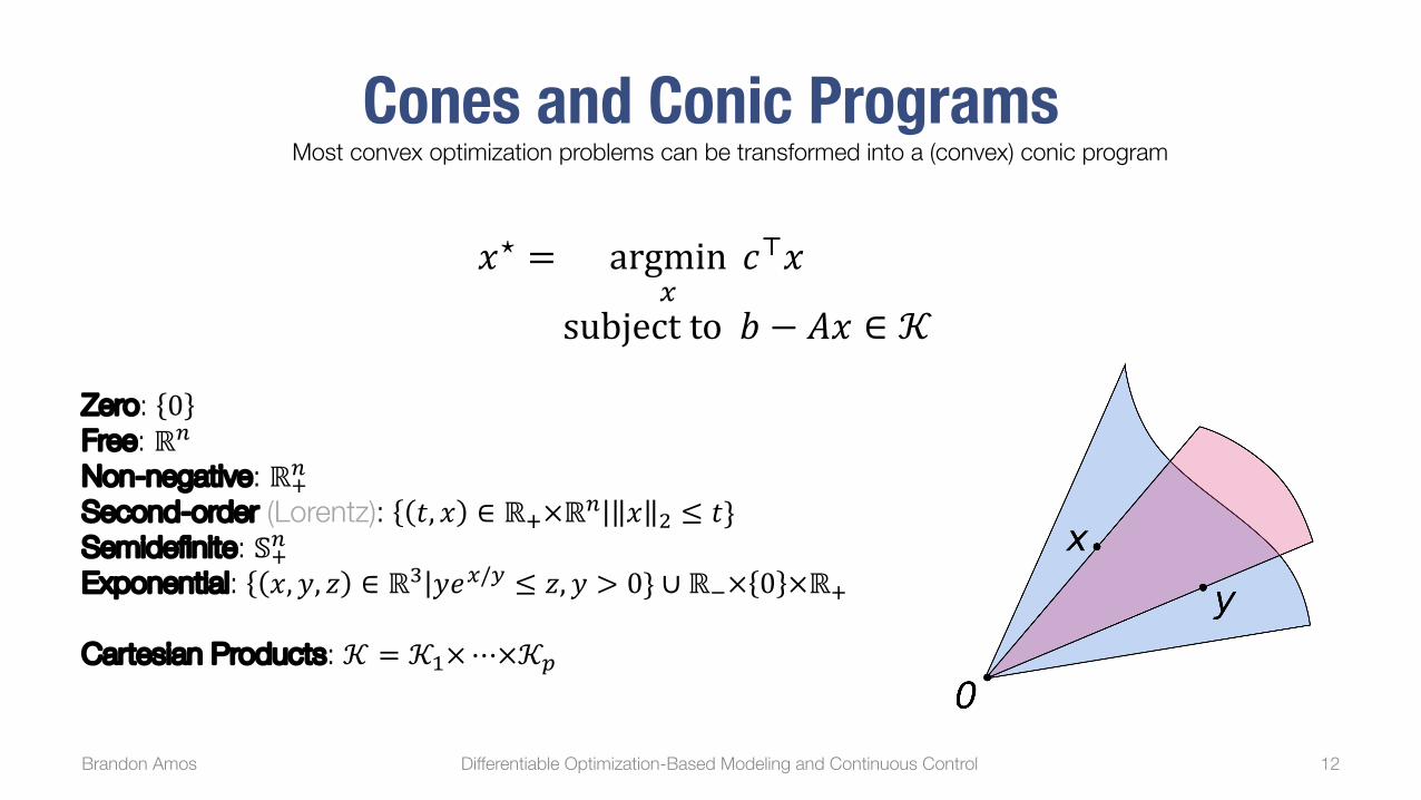
Optimization layers need to be carefully implemented


Algorithm 1 Differentiable LQR Module (The LQR algorithm is defined in Appendix A)

Input: Initial state xinit

Parameters: ✓ = {C, c, F, f}

Forward Pass:

1: ⌧?1:T = LQRT (xinit;C, c, F, f) . Solve (2)

2: Compute �?1:T with (7)

Backward Pass:

1: d?⌧1:T = LQRT (0;C,r⌧?

t`, F, 0) . Solve (9), reusing the factorizations from the forward pass

2: Compute d?�1:T

with (7)3: Compute the derivatives of ` with respect to C, c, F , f , and xinit with (8)

where the initial constraint x1 = xinit is represented by setting F0 = 0 and f0 = xinit. DifferentiatingEquation (4) with respect to ⌧

?t yields

r⌧tL(⌧?,�?) = Ct⌧?t + Ct + F

>t �

?t �

�?t�10

�= 0, (5)

Thus, the normal approach to solving LQR problems with dynamic Riccati recursion can be viewedas an efficient way of solving the following KKT system

Kz }| {⌧t �t ⌧t+1 �t+12

6666666664

. . .Ct F

>t

Ft [�I 0]�I

0

�Ct+1 F

>t+1

Ft+1

. . .

3

7777777775

2

66666664

...⌧?t�?t

⌧?t+1

�?t+1...

3

77777775

= �

2

66666664

...ctftct+1ft+1

...

3

77777775

. (6)

Given an optimal nominal trajectory ⌧?1:T , Equation (5) shows how to compute the optimal dual

variables � with the backward recursion�?T = CT,x⌧

?T + cT,x, �

?t = F

>t,x�

?t+1 + Ct,x⌧

?t + ct,x, (7)

where Ct,x, ct,x, and Ft,x are the first block-rows of Ct, ct, and Ft, respectively. Now that we havethe optimal trajectory and dual variables, we can compute the gradients of the loss with respect tothe parameters. Since LQR is a constrained convex quadratic argmin, the derivatives of the losswith respect to the LQR parameters can be obtained by implicitly differentiating the KKT conditions.Applying the approach from Section 3 of Amos and Kolter [2017], the derivatives are

@`

@Ct=

1

2

�d?⌧t ⌦ ⌧

?t + ⌧

?t ⌦ d

?⌧t

� @`

@ct= d

?⌧t

@`

@xinit= d

?�0

@`

@Ft= d

?�t+1

⌦ ⌧?t + �

?t+1 ⌦ d

?⌧t

@`

@ft= d

?�t

(8)

where ⌦ is the outer product operator, and d?⌧ and d

?� are obtained by solving the linear system

K

2

6664

...d?⌧t

d?�t

...

3

7775= �

2

6664

...r⌧?

t`

0...

3

7775. (9)

We observe that Equation (9) is of the same form as the linear system in Equation (6) for the LQRproblem. Therefore, we can leverage this insight and solve Equation (9) efficiently by solving anotherLQR problem that replaces ct with r⌧?

t` and ft with 0. Moreover, this approach enables us to re-use

the factorization of K from the forward pass instead of recomputing. Algorithm 1 summarizes theforward and backward passes for a differentiable LQR module.

4




Forward Pass:



Backward Pass:

1: d?⌧1:T = LQRT (0;C,r⌧?


2: Compute d?�1:T



?t yields

r⌧tL(⌧?,�?) = Ct⌧?t + Ct + F

>t �

?t �

�?t�10

�= 0, (5)


Kz }| {⌧t �t ⌧t+1 �t+12

6666666664

. . .Ct F

>t

Ft [�I 0]�I

0

�Ct+1 F

>t+1

Ft+1

. . .

3

7777777775

2

66666664

...⌧?t�?t

⌧?t+1

�?t+1...

3

77777775

= �

2

66666664

...ctftct+1ft+1

...

3

77777775

. (6)



?T + cT,x, �

?t = F

>t,x�

?t+1 + Ct,x⌧

?t + ct,x, (7)


@`

@Ct=

1

2

�d?⌧t ⌦ ⌧

?t + ⌧

?t ⌦ d

?⌧t

� @`

@ct= d

?⌧t

@`

@xinit= d

?�0

@`

@Ft= d

?�t+1

⌦ ⌧?t + �

?t+1 ⌦ d

?⌧t

@`

@ft= d

?�t

(8)



K

2

6664

...d?⌧t

d?�t

...

3

7775= �

2

6664

...r⌧?

t`

0...

3

7775. (9)




4




Forward Pass:



Backward Pass:

1: d?⌧1:T = LQRT (0;C,r⌧?


2: Compute d?�1:T



?t yields

r⌧tL(⌧?,�?) = Ct⌧?t + Ct + F

>t �

?t �

�?t�10

�= 0, (5)


Kz }| {⌧t �t ⌧t+1 �t+12

6666666664

. . .Ct F

>t

Ft [�I 0]�I

0

�Ct+1 F

>t+1

Ft+1

. . .

3

7777777775

2

66666664

...⌧?t�?t

⌧?t+1

�?t+1...

3

77777775

= �

2

66666664

...ctftct+1ft+1

...

3

77777775

. (6)



?T + cT,x, �

?t = F

>t,x�

?t+1 + Ct,x⌧

?t + ct,x, (7)


@`

@Ct=

1

2

�d?⌧t ⌦ ⌧

?t + ⌧

?t ⌦ d

?⌧t

� @`

@ct= d

?⌧t

@`

@xinit= d

?�0

@`

@Ft= d

?�t+1

⌦ ⌧?t + �

?t+1 ⌦ d

?⌧t

@`

@ft= d

?�t

(8)



K

2

6664

...d?⌧t

d?�t

...

3

7775= �

2

6664

...r⌧?

t`

0...

3

7775. (9)




4

Why should practitioners care?


Differentiable convex optimization layers


NeurIPS 2019 (and officially in CVXPY!)Joint work with A. Agrawal, S. Barratt, S. Boyd, S. Diamond, J. Z. Kolter

locuslab.github.io/2019-10-28-cvxpylayers

A new way of rapidly prototyping optimization layers


…Inputs Losscvxpy optimization layer

!"#$ = argmin,

-.(!, !")s.t. ! ∈ ∁.(!")

Backprop

…

Parameters

Variables

Constants

CanonicalizedCone Program

argmin7

89:s.t. ;: ≼= >

Problem

ObjectiveConstraints

Cone ProgramSolution

Original ProblemSolution

This TalkFoundation: Differentiable convex optimization

Differentiable continuous controlDifferentiable model predictive controlDifferentiable cross-entropy method


Should RL policies have a system dynamics model or not?

Model-free RLMore general, doesn’t make as many assumptions about the worldRife with poor data efficiency and learning stability issues

Model-based RL (or control)A useful prior on the world if it lies within your set of assumptions


State Action

Policy Neural Network(s)

Future Plan

System Dynamics

Model Predictive Control


Known or learned from data

The Objective Mismatch Problem


Dynamics !" Policy #"(%) Environment

State Transitions RewardTrajectories

Training: Maximum Likelihood Objective Mismatch

Control Interacts

Responses

Differentiable Model Predictive ControlApureplanningproblemgiven(potentiallynon-convex)cost anddynamics:


𝜏#:3⋆ = argmin4!:#

b5

𝐶%(𝜏5)

subject to 𝑥# = 𝑥init𝑥5"# = 𝑓% 𝜏5𝑢 ≤ 𝑢 ≤ 𝑢

Cost

Dynamics

where𝜏! = {𝑥! , 𝑢!}

Idea: Differentiatethroughthisoptimizationproblem

Differentiable Model Predictive Control


Layer z"… MPC Layer …


What can we do with this now?Augment neural network policies in model-free algorithms with MPC policiesReplace the unrolled controllers in other settings (hindsight plan, universal planning networks)Fight objective mismatch by end-to-end learning dynamicsThe cost can also be end-to-end learned! No longer need to hard-code in values

Approach 1: Differentiable MPC/iLQR


Can differentiate through the chain of QPs or just the last one if it’s a fixed point

Differentiating LQR with LQR


Solving LQR with dynamic Riccati recursion efficiently solves the KKT system




Forward Pass:



Backward Pass:

1: d?⌧1:T = LQRT (0;C,r⌧?


2: Compute d?�1:T



?t yields

r⌧tL(⌧?,�?) = Ct⌧?t + Ct + F

>t �

?t �

�?t�10

�= 0, (5)


Kz }| {⌧t �t ⌧t+1 �t+12

6666666664

. . .Ct F

>t

Ft [�I 0]�I

0

�Ct+1 F

>t+1

Ft+1

. . .

3

7777777775

2

66666664

...⌧?t�?t

⌧?t+1

�?t+1...

3

77777775

= �

2

66666664

...ctftct+1ft+1

...

3

77777775

. (6)



?T + cT,x, �

?t = F

>t,x�

?t+1 + Ct,x⌧

?t + ct,x, (7)


@`

@Ct=

1

2

�d?⌧t ⌦ ⌧

?t + ⌧

?t ⌦ d

?⌧t

� @`

@ct= d

?⌧t

@`

@xinit= d

?�0

@`

@Ft= d

?�t+1

⌦ ⌧?t + �

?t+1 ⌦ d

?⌧t

@`

@ft= d

?�t

(8)



K

2

6664

...d?⌧t

d?�t

...

3

7775= �

2

6664

...r⌧?

t`

0...

3

7775. (9)




4




Forward Pass:



Backward Pass:

1: d?⌧1:T = LQRT (0;C,r⌧?


2: Compute d?�1:T



?t yields

r⌧tL(⌧?,�?) = Ct⌧?t + Ct + F

>t �

?t �

�?t�10

�= 0, (5)


Kz }| {⌧t �t ⌧t+1 �t+12

6666666664

. . .Ct F

>t

Ft [�I 0]�I

0

�Ct+1 F

>t+1

Ft+1

. . .

3

7777777775

2

66666664

...⌧?t�?t

⌧?t+1

�?t+1...

3

77777775

= �

2

66666664

...ctftct+1ft+1

...

3

77777775

. (6)



?T + cT,x, �

?t = F

>t,x�

?t+1 + Ct,x⌧

?t + ct,x, (7)


@`

@Ct=

1

2

�d?⌧t ⌦ ⌧

?t + ⌧

?t ⌦ d

?⌧t

� @`

@ct= d

?⌧t

@`

@xinit= d

?�0

@`

@Ft= d

?�t+1

⌦ ⌧?t + �

?t+1 ⌦ d

?⌧t

@`

@ft= d

?�t

(8)



K

2

6664

...d?⌧t

d?�t

...

3

7775= �

2

6664

...r⌧?

t`

0...

3

7775. (9)




4




Forward Pass:



Backward Pass:

1: d?⌧1:T = LQRT (0;C,r⌧?


2: Compute d?�1:T



?t yields

r⌧tL(⌧?,�?) = Ct⌧?t + Ct + F

>t �

?t �

�?t�10

�= 0, (5)


Kz }| {⌧t �t ⌧t+1 �t+12

6666666664

. . .Ct F

>t

Ft [�I 0]�I

0

�Ct+1 F

>t+1

Ft+1

. . .

3

7777777775

2

66666664

...⌧?t�?t

⌧?t+1

�?t+1...

3

77777775

= �

2

66666664

...ctftct+1ft+1

...

3

77777775

. (6)



?T + cT,x, �

?t = F

>t,x�

?t+1 + Ct,x⌧

?t + ct,x, (7)


@`

@Ct=

1

2

�d?⌧t ⌦ ⌧

?t + ⌧

?t ⌦ d

?⌧t

� @`

@ct= d

?⌧t

@`

@xinit= d

?�0

@`

@Ft= d

?�t+1

⌦ ⌧?t + �

?t+1 ⌦ d

?⌧t

@`

@ft= d

?�t

(8)



K

2

6664

...d?⌧t

d?�t

...

3

7775= �

2

6664

...r⌧?

t`

0...

3

7775. (9)




4

Backwards Pass: Implicitly differentiate the LQR KKT conditions:

where

Just another LQR problem!

Approach 2: The Cross-Entropy Method


Iterative sampling-based optimizer that:

1. Samples from the domain2. Observes the function’s values3. Updates the sampling distribution

SOTA optimizer for control and model-based RL

The Differentiable Cross-Entropy Method (DCEM)


Differentiate backwards through the sequence of samples- Using differentiable top-k (LML) and reparameterization

Useful when a fixed point is hard to find, or when unrolling gradient descent hits a local optimum

A differentiable controller in the RL setting


sites.google.com/view/diff-cross-entropy-method

DCEM fine-tunes highly non-convex controllers

https://sites.google.com/view/diff-cross-entropy-method/home

DCEM can exploit the solution space structure


Full Domain

Manifold ofOptimal Solutions

𝑥⋆ = argmin/∈ 1,2 !

𝑓 𝑥

Latent Manifoldof Optimal Solutions

Brandon Amos • Facebook AI Research

Differentiable Optimization-Based Modeling and Continuous Control

• Differentiable QPs: OptNet [ICML 2017]• Differentiable Stochastic Opt: Task-based Model Learning [NeurIPS 2017]• Differentiable MPC for End-to-end Planning and Control [NeurIPS 2018]• Differentiable Convex Optimization Layers [NeurIPS 2019]• Differentiable Optimization-Based Modeling for ML [Ph.D. Thesis 2019]• Differentiable Top-k and Multi-Label Projection [arXiv 2019]• Objective Mismatch in Model-based Reinforcement Learning [L4DC 2020]• Differentiable Cross-Entropy Method [ICML 2020]

Joint with Akshay Agrawal, Shane Barratt, Byron Boots, Stephen Boyd, Roberto Calandra, Steven Diamond, Priya Donti, Ivan Jimenez, Zico Kolter, Vladlen Koltun, Nathan Lambert, Jacob Sacks, Omry Yadan, and Denis Yarats

https://arxiv.org/abs/1703.00443

http://papers.nips.cc/paper/7132-task-based-end-to-end-model-learning-in-stochastic-optimization

http://papers.nips.cc/paper/9152-differentiable-convex-optimization-layers

https://github.com/bamos/thesis




On differentiable optimization for control ... - Brandon Amos

Documents

Transcript of On differentiable optimization for control ... - Brandon Amos