C3.3 Differentiable Manifolds

C3.3 Differentiable Manifolds*

Prof Jason D. Lotay

[email protected]

Balliol College 3.7

Michaelmas Term 2021–2022

Course overview

A manifold is a space such that small pieces of it look like small pieces of Euclidean space. Thus a

smooth surface is an example of a (2-dimensional) manifold. Manifolds are the natural setting for parts

of classical applied mathematics such as mechanics, as well as general relativity. They are also central to

areas of pure mathematics such as topology and certain aspects of analysis.

In this course we introduce the tools needed to do analysis on manifolds, including vector fields, differential

forms and the notion of orientability. We prove a very general form of Stokes’ Theorem which includes

as special cases the classical theorems of Gauss, Green and Stokes. We also introduce the theory of de

Rham cohomology, which is central to many arguments in topology. In particular, we discuss the central

notion of degree of smooth maps between manifolds, and its applications. Finally, we briefly discuss

Riemannian manifolds, including Riemannian metrics, isometries and geodesics.

Prerequisities. A good understanding of basic topology (e.g. the notions of Hausdorff, open cover,

compact, connected etc.) and the theory of smooth functions from Rn to Rm (including the definition

of the differential and the Inverse and Implicit Function Theorems) will be assumed. It will be helpful if

you have studied surfaces (both in R3 and “abstract” surfaces), but not essential.

Disclaimer. These lecture notes cover the essential course material (and a bit more), but there are no

pictures and possibly a few typos. The lectures will provide additional motivation and intuition which

will be invaluable for understanding and appreciating the material. Moreover, I would suggest combining

these lecture notes with material from the recommended reading below.

Recommended texts

D. Barden and C. Thomas, An Introduction to Differential Manifolds. (Imperial College Press,

London, 2003.)

M. Berger and B. Gostiaux, Differential Geometry: Manifolds, Curves and Surfaces. Translated

from the French by S. Levy, (Springer Graduate Texts in Mathematics, 115, Springer–Verlag (1988))

Chapters 0-3, 5-7.

W. Boothby, An Introduction to Differentiable Manifolds and Riemannian Geometry, 2nd edition,

(Academic Press, 1986).

M. Spivak, Calculus on Manifolds, (W. A. Benjamin, 1965).

M. Spivak, A Comprehensive Introduction to Differential Geometry, Vol. 1, (1970).

F. Warner, Foundations of Differentiable Manifolds and Lie Groups, (Springer Graduate Texts in

Mathematics, 1994).

The best books for the course are probably Barden and Thomas, Boothby and Spivak (Calculus on

Manifolds).

*This version: December 7, 2021.

1

Jason D. Lotay C3.3 Differentiable Manifolds

Contents

1 Manifolds: definition and examples 4

1.1 Basic examples . . . . . . . . . . . . . . . . . . . . . . . . . . . . . . . . . . . . . . . . . . 4

1.2 Some non-examples . . . . . . . . . . . . . . . . . . . . . . . . . . . . . . . . . . . . . . . . 5

1.3 More advanced examples . . . . . . . . . . . . . . . . . . . . . . . . . . . . . . . . . . . . . 5

1.4 Constructing manifolds: regular values . . . . . . . . . . . . . . . . . . . . . . . . . . . . . 6

1.5 The formal definition . . . . . . . . . . . . . . . . . . . . . . . . . . . . . . . . . . . . . . . 8

1.6 Smooth maps . . . . . . . . . . . . . . . . . . . . . . . . . . . . . . . . . . . . . . . . . . . 11

1.7 Quotient constructions . . . . . . . . . . . . . . . . . . . . . . . . . . . . . . . . . . . . . . 13

2 Tangent vectors 16

2.1 Tangent vectors and regular values . . . . . . . . . . . . . . . . . . . . . . . . . . . . . . . 16

2.2 Tangent vectors as differential operators . . . . . . . . . . . . . . . . . . . . . . . . . . . . 18

2.3 Differential . . . . . . . . . . . . . . . . . . . . . . . . . . . . . . . . . . . . . . . . . . . . 19

2.4 Local diffeomorphisms . . . . . . . . . . . . . . . . . . . . . . . . . . . . . . . . . . . . . . 20

2.5 Regular values . . . . . . . . . . . . . . . . . . . . . . . . . . . . . . . . . . . . . . . . . . 21

2.6 Immersions, embeddings and submersions . . . . . . . . . . . . . . . . . . . . . . . . . . . 22

3 Vector fields 24

3.1 Tangent bundle . . . . . . . . . . . . . . . . . . . . . . . . . . . . . . . . . . . . . . . . . . 24

3.2 Definition of vector fields . . . . . . . . . . . . . . . . . . . . . . . . . . . . . . . . . . . . 25

3.3 Parallelizable manifolds . . . . . . . . . . . . . . . . . . . . . . . . . . . . . . . . . . . . . 26

3.4 Pushforward . . . . . . . . . . . . . . . . . . . . . . . . . . . . . . . . . . . . . . . . . . . . 27

3.5 Lie bracket . . . . . . . . . . . . . . . . . . . . . . . . . . . . . . . . . . . . . . . . . . . . 28

3.6 Integral curves . . . . . . . . . . . . . . . . . . . . . . . . . . . . . . . . . . . . . . . . . . 29

3.7 Flow . . . . . . . . . . . . . . . . . . . . . . . . . . . . . . . . . . . . . . . . . . . . . . . . 31

3.8 Lie derivative . . . . . . . . . . . . . . . . . . . . . . . . . . . . . . . . . . . . . . . . . . . 32

4 Differential forms 34

4.1 Vector bundles . . . . . . . . . . . . . . . . . . . . . . . . . . . . . . . . . . . . . . . . . . 34

4.2 Exterior algebra . . . . . . . . . . . . . . . . . . . . . . . . . . . . . . . . . . . . . . . . . 35

4.3 Forms on manifolds . . . . . . . . . . . . . . . . . . . . . . . . . . . . . . . . . . . . . . . . 37

4.4 Pullback . . . . . . . . . . . . . . . . . . . . . . . . . . . . . . . . . . . . . . . . . . . . . . 39

4.5 Exterior derivative . . . . . . . . . . . . . . . . . . . . . . . . . . . . . . . . . . . . . . . . 40

4.6 Lie derivative and Cartan’s formula . . . . . . . . . . . . . . . . . . . . . . . . . . . . . . . 42

5 Orientation 45

5.1 Partitions of unity . . . . . . . . . . . . . . . . . . . . . . . . . . . . . . . . . . . . . . . . 45

5.2 Orientability and volume forms . . . . . . . . . . . . . . . . . . . . . . . . . . . . . . . . . 47

6 Integration 51

6.1 Integration on manifolds . . . . . . . . . . . . . . . . . . . . . . . . . . . . . . . . . . . . . 51

6.2 Manifolds with boundary . . . . . . . . . . . . . . . . . . . . . . . . . . . . . . . . . . . . 54

6.3 Stokes Theorem . . . . . . . . . . . . . . . . . . . . . . . . . . . . . . . . . . . . . . . . . . 55

7 De Rham cohomology and applications 59

7.1 De Rham cohomology: definition and properties . . . . . . . . . . . . . . . . . . . . . . . 59

7.2 Examples . . . . . . . . . . . . . . . . . . . . . . . . . . . . . . . . . . . . . . . . . . . . . 61

7.3 Degree . . . . . . . . . . . . . . . . . . . . . . . . . . . . . . . . . . . . . . . . . . . . . . . 67

2


8 Riemannian manifolds 72

8.1 Definition . . . . . . . . . . . . . . . . . . . . . . . . . . . . . . . . . . . . . . . . . . . . . 72

8.2 Examples . . . . . . . . . . . . . . . . . . . . . . . . . . . . . . . . . . . . . . . . . . . . . 72

8.3 Pullback and existence of Riemannian metrics . . . . . . . . . . . . . . . . . . . . . . . . . 73

8.4 Forms and the Hodge star . . . . . . . . . . . . . . . . . . . . . . . . . . . . . . . . . . . . 74

8.5 Isometries and Killing fields . . . . . . . . . . . . . . . . . . . . . . . . . . . . . . . . . . . 76

8.6 Geodesics . . . . . . . . . . . . . . . . . . . . . . . . . . . . . . . . . . . . . . . . . . . . . 78

8.7 Harmonic forms: not examinable . . . . . . . . . . . . . . . . . . . . . . . . . . . . . . . . 83

3


1 Manifolds: definition and examples

We want to start by talking about one of the key building blocks of modern geometry: manifolds. All of

the manifolds we will discuss, as the name of this course suggests, will be differentiable manifolds, and

so we will omit the adjective “differentiable” for simplicity (as is standard practice in this area).

For the moment, let us make a fake definition of manifold and see some examples.

First fake definition: A manifold is the natural notion of a smooth object.

Although this definition is fake, it is useful in the sense that everything that you would imagine to

be a smooth object (and thus a manifold) is a manifold. Moreover, the actual definition is not very

enlightening. We need it, so that all of the theory makes sense, but once we have it we then very rarely

need to use it.

1.1 Basic examples

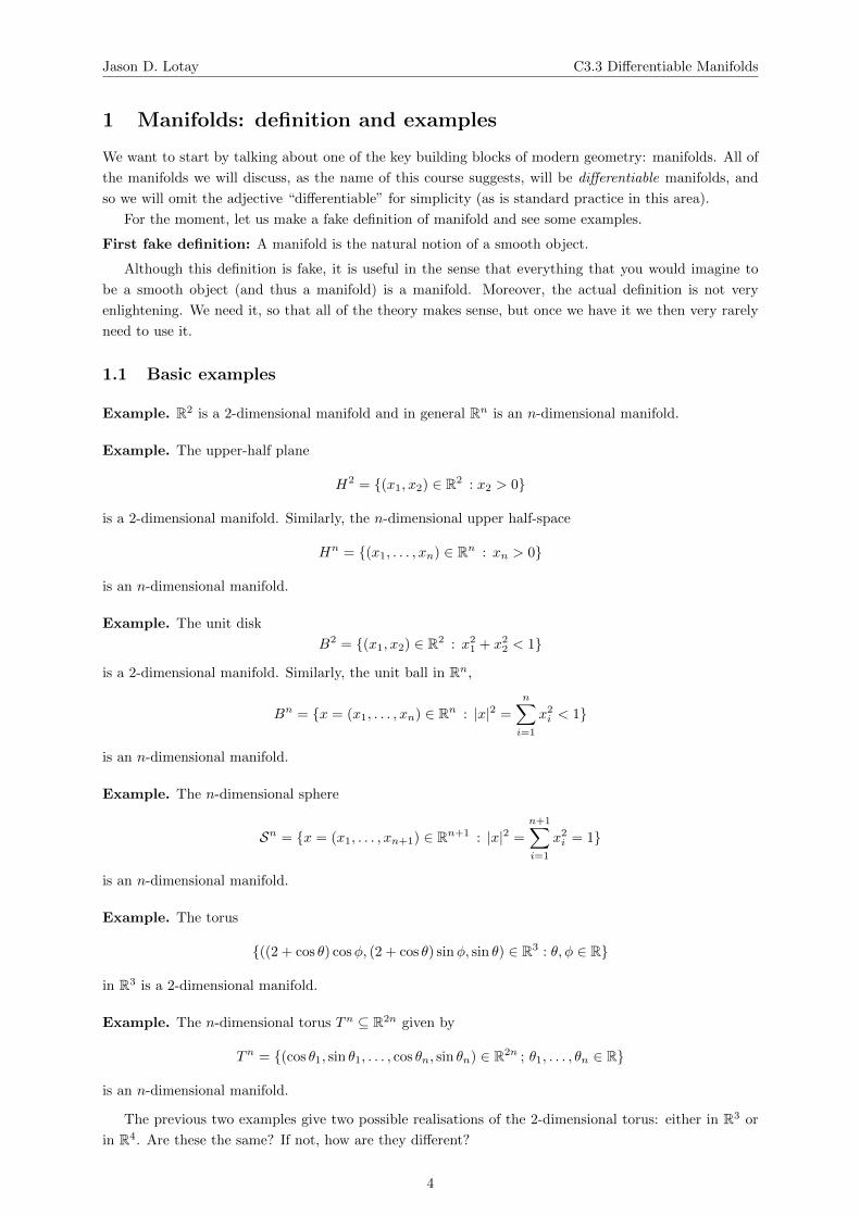
Example. R2 is a 2-dimensional manifold and in general Rn is an n-dimensional manifold.

Example. The upper-half plane

H2 = (x1, x2) ∈ R2 : x2 > 0

is a 2-dimensional manifold. Similarly, the n-dimensional upper half-space

Hn = (x1, . . . , xn) ∈ Rn : xn > 0

is an n-dimensional manifold.

Example. The unit disk

B2 = (x1, x2) ∈ R2 : x21 + x22 < 1

is a 2-dimensional manifold. Similarly, the unit ball in Rn,

Bn = x = (x1, . . . , xn) ∈ Rn : |x|2 =

n∑i=1

x2i < 1


Example. The n-dimensional sphere

Sn = x = (x1, . . . , xn+1) ∈ Rn+1 : |x|2 =

n+1∑i=1

x2i = 1


Example. The torus

((2 + cos θ) cosϕ, (2 + cos θ) sinϕ, sin θ) ∈ R3 : θ, ϕ ∈ R

in R3 is a 2-dimensional manifold.

Example. The n-dimensional torus Tn ⊆ R2n given by

Tn = (cos θ1, sin θ1, . . . , cos θn, sin θn) ∈ R2n ; θ1, . . . , θn ∈ R


The previous two examples give two possible realisations of the 2-dimensional torus: either in R3 or

in R4. Are these the same? If not, how are they different?

4


1.2 Some non-examples

So what is a manifold? The simplest example of an n-dimensional manifold that we have seen is just Rn,and this is the local model for all manifolds.

Second fake definition: An n-dimensional manifold is something which locally “looks like” Rn (but

globally can be much more interesting).

For example, if you take a sphere in R3, it is clearly not just flat R2, but if you look near any given

point you can define coordinates so it looks like a piece of R2. The same trick can be done for all of the

examples we have seen so far. With this second fake definition we may ask the question: what is not a

manifold?

Example. A cube is not a manifold. It is not smooth at the edges and at the corners. Indeed, it looks

like R2 on the faces, but not at the edges or at the corners.

Similarly, any polyhedron is not a manifold.

Example. The closed disk in R2

x ∈ R2 : |x| ≤ 1

is not quite a 2-dimensional manifold because it looks like R2 in the interior where |x| < 1, but when

|x| = 1 we have the circle S1. (However, it is what is called a 2-dimensional manifold with boundary.)

Example. The hyperboloid of one sheet

(x1, x2, x3) ∈ R3 : x21 + x22 − x23 = 1

and the hyperboloid of two sheets

(x1, x2, x3) ∈ R3 : x21 + x22 − x23 = −1

are 2-dimensional manifolds, but

(x1, x2, x3) ∈ R3 : x21 + x22 − x23 = 0

is a cone and so is not a manifold, because it is not smooth at 0, or it does not look like R2 there.

1.3 More advanced examples

Now, everything we have looked at so far has been quite concrete, but one of the great powers of the

theory of manifolds is that they include much more abstract objects. Let us now look at two more

abstract things, which I claim are manifolds, and we shall see why shortly.

Example. Let Mn(R) be the n× n real matrices. Then the general linear group is

GL(n,R) = A ∈Mn(R) : detA = 0

and the special linear group is

SL(n,R) = A ∈Mn(R) : detA = 1.

(Notice that these are groups under multiplication because the identity matrix is in both, and det(AB) =

detAdetB.) Then GL(n,R) is an n2-dimensional manifold and SL(n,R) is an n2 − 1-dimensional mani-

fold.

Example. Let I be the identity matrix in Mn(R). Then

O(n) = A ∈Mn(R) : ATA = I and SO(n) = A ∈ O(n) : det(A) = 1

5


are the orthogonal and special orthogonal group, respectively. (Again, notice that these are groups

under multiplication because I is in both and (AB)T(AB) = BTATAB.) Then O(n) and SO(n) are12n(n− 1)-dimensional manifolds.

Example. Let

SU(2) =

(a b

−b a

): a, b ∈ C, |a|2 + |b|2 = 1

.

This is again a group and is a 3-dimensional manifold. In general, if we let Mn(C) be the n× n complex

matrices, then the special unitary group

SU(n) =A ∈Mn(C) : ATA = I, detA = 1

is an n2 − 1-dimensional manifold and the unitary group

U(n) =A ∈Mn(C) : ATA = I

is an n2-dimensional manifold. (These are, sort of, complex analogues of the special orthogonal and

orthogonal groups.)

Remark. The examples just given in terms of matrices are all examples of manifolds which are groups:

in fact, this is almost the definition of a Lie group (we will see the correct definition later), and these

examples are indeed all Lie groups.

We can even go a bit more abstract, and produce some more interesting spaces which play an important

role in the study of manifolds.

Example. Let RPn be the set of straight lines in Rn+1 through 0. Then RPn is the real projective

n-space and is an n-dimensional manifold.

We can equivalently say that RPn is the quotient of Rn+1 \ 0 by the equivalence relation x ∼ y

if x = λy for some λ ∈ R. Hence, we usually denote points in RPn (which represent lines in Rn+1) by

equivalence classes [x] (where x ∈ Rn+1 \ 0 lies on the line).

Example. We have that Cn is a 2n-dimensional manifold. We can then consider the set CPn of complex

lines in Cn+1 through 0. This is also a 2n-dimensional manifold, called complex projective n-space.

More explicitly, CPn is the quotient of Cn+1 \ 0 by the equivalence relation z ∼ w if z = λw for

some λ ∈ C. Again, we tend to denote points in CPn by equivalence classes [z].

1.4 Constructing manifolds: regular values

Let us put off the formal definition of manifold a little bit longer and give a general technique for

constructing manifolds which is very helpful.

Recall: If we write F : Rn → Rm as F (x) = (F1(x), . . . , Fm(x)) then the derivative of F at p is the

linear map dFp : Rn → Rm which is represented by the matrix (∂Fi

∂xj(p)). In general, dFp is the linear

map so that|F (p+ h)− F (p)− dFp(h)|

|h|→ 0 as |h| → 0.

Remark. We will say that a map is smooth if it is infinitely differentiable (i.e. C∞). Many statements

we make in this course can naturally be generalised to the case where maps have weaker differentiability

properties, but in this course we will restrict ourselves to the smooth category.

6


Theorem 1.1. (Regular value theorem). Let F : Rn+m → Rm be a smooth map and suppose that

for all p ∈ F−1(c), where

F−1(c) = p ∈ Rn+m : F (p) = c = ∅,

the derivative dFp : Rn+m → Rm is surjective (i.e. c is a regular value of F ). Then F−1(c) is an

n-dimensional manifold.

Remark. This would obviously work just as well if F is only defined on an open set in Rn+m.

Let us put this theorem to use straight away.

Example. Let F : Rn+1 → R be

F (x1, . . . , xn+1) =

n+1∑i=1

x2i .

Notice that F is a smooth map (since it is polynomial) with

dFx = (2x1 . . . 2xn+1).

If x ∈ F−1(1) then dFx = 0, but if x ∈ F−1(0) then dFx = 0. In this case, the derivative being non-zero

is equivalent to saying that the map dFx : Rn+1 → R is surjective, so 1 is a regular value but 0 is not.

Hence, by Theorem 1.1, we see that F−1(1) = Sn is an (n + 1) − 1 = n-dimensional manifold. We

also notice that F−1(0) = 0, which is obviously not an n-dimensional manifold.

Example. Let F : R2n → Rn be

F (x1, . . . , x2n) = (x21 + x22 − 1, . . . , x22n−1 + x22n − 1).

This is a smooth map and for x ∈ F−1(0),

dFx =

2x1 2x2 0 0 . . . 0 0

0 0 2x3 2x4 . . . 0 0...

......

... . . ....

...

0 0 0 0 . . . 2x2n−1 2x2n

has rank n as a matrix because the rows are all linearly independent, as (x2i−1, x2i) = (0, 0) for all i.

We deduce that dFx is a surjective map. Thus F−1(0) = Tn ⊆ R2n is an n-dimensional manifold by

Theorem 1.1.

Our next example shows that, although being a regular value of a function is a sufficient condition to

ensure that the level set is a manifold, it is not necessary.

Example. Let F (x1, x2) = x31 − x32. Then dF(x1,x2) = (3x21 − 3x22) so 0 is not a regular value of F

because dF(0,0) = 0. However

F−1(0) = (x1, x2) ∈ R2 : x31 = x32 = (x1, x1) ∈ R2 : x1 ∈ R

which is a 1-dimensional manifold (just a diagonal line in the plane).

We now give a more sophisticated implementation of Theorem 1.1.

Example. Define F :Mn(R) →Mn(R) by F (A) = ATA− I. Notice that F (A)T = F (A), so F actually

maps into Symn(R), the symmetric n×n matrices. Notice that Mn(R) ∼= Rn2

and Symn(R) ∼= R 12n(n+1).

Clearly F is smooth and we compute its derivative, which is the part of F (A+B)−F (A) which is linear

in B. Explicitly, we see that

F (A+B)− F (A) = (A+B)T(A+B)−ATA = BTA+ATB +BTB.

7


Hence,|F (A+B)− F (A)− (BTA+ATB)|

|B|=

|BTB||B|

→ 0

as |B| → 0, so

dFA(B) = BTA+ATB.

If C ∈ Symn(R) and A ∈ F−1(0) then, since CT = C and ATA = I, we have

dFA(1

2AC) =

1

2(AC)TA+

1

2ATAC =

1

2CTATA+

1

2C = C,

so dFA is surjective. Applying Theorem 1.1 gives that O(n) = F−1(0) is an n2 − 12n(n+1) = 1

2n(n− 1)-

dimensional manifold.

Notice that O(n) is the disjoint union of two manifolds because for all A ∈ O(n), det(A) = ±1, so

SO(n) is an open subset of O(n), and hence is also an 12n(n − 1)-dimensional manifold. You can also

show this directly using the same argument as above replacing Mn(R) by the open subset GL+(n,R) =A ∈Mn(R) : detA > 0.

Remark. Theorem 1.1 is extremely helpful. For example, it says that, most of the time, if you look

at the zero set of a system of polynomials you will get a manifold if the system has a root. This

is particularly helpful in complex Euclidean space (or complex projective space, as long as you use

homogeneous polynomials), since complex polynomials always have roots (by the Fundamental Theorem

of Algebra). Zero sets of systems of polynomials in complex projective space are important objects in

algebraic geometry.

1.5 The formal definition

The formal definition of a manifold may look a bit strange but the key points we want are:

“abstract” objects – e.g. the usual torus in R3 we know should be “the same” as T 2 = S1×S1 ⊆ R4;

smooth geometric objects – e.g. we want things like the sphere but we want to rule out the cube

and the cone;

objects on which we can measure how quantities vary as we move from point to point – i.e. we can

define differentation.

With these properties, the definition of manifold becomes essentially determined.

Definition 1.2. An n-dimensional manifold is a (second countable, Hausdorff) topological spaceM such

that there exists a family A = (Ui, φi) : i ∈ I where:

Ui is an open set in M and ∪i∈IUi =M ;

φi : Ui → Rn is a continuous bijection onto an open set φi(Ui) with continuous inverse (i.e. a

homeomorphism);

whenever Ui∩Uj = ∅, the transition map φj φ−1i : φi(Ui∩Uj) → φj(Ui∩Uj) is a smooth (infinitely

differentiable) bijection with smooth inverse (i.e. a diffeomorphism).

The family A is called an atlas and the pairs (Ui, φi) are called (coordinate) charts. (We are pasting

together little flat maps to get a picture of a non-flat object, just like with the Earth.)

Remark. (Not examinable). Second countable means there is a countable collection of open sets

which form a basis for all open sets: for Rn, for example, we can take the set of balls Br(x) with centre

x ∈ Qn and radius r ∈ Q+. Recall that Hausdorff means that for any distinct points x and y we can

find disjoint open sets containing x and y. Almost every example of a manifold in this course will come

8


from a metric space, where second countable is the same thing as separable. Separable means there is a

countable dense subset: for Rn just take Qn as the countable dense subset (dense just means its closure

is the whole space, or every non-empty open set meets the dense set). Since our emphasis is on geometry,

we will not worry about these sort of topological issues in this course.

Remark. (Not examinable). One can also weaken the definition of manifold by requiring less differ-

entiability for the transition maps, or by relaxing the topological assumptions (e.g. dropping the second

countable requirement), but this will mean that certain constructions that arise in this course are not

possible or need to be adapted.

As we already said, most of the time we do not need the definition of manifold: we just need to know

that something is one. As we have seen, everything you would like to be a manifold is one. However, it

is instructive to check that some things really fit the definition of manifold.

Let us now try to give some examples of manifolds from the definition.

Example. Rn is an n-dimensional manifold: take U = Rn, φ = id (the identity map) and A = (U,φ).The same works for any open set in Rn, so this shows that Hn and Bn are n-dimensional manifolds.

Example. In fact, any open subset U of a manifold M is a manifold of the same dimension – take the

atlas (Ui ∩ U,φi|Ui∩U ) : i ∈ I if (Ui, φi) : i ∈ I is an atlas for M .

In particular since Mn(R) = Rn2

(we have n2 independent real entries in the matrix) and GL(n,R) isan open set in Mn(R) (since the condition detA = 0 is an open condition), we have that GL(n,R) andGL+(n,R) are n2-dimensional manifolds.

Example. Consider Sn.

Let N = (0, . . . , 0, 1) and S = (0, . . . , 0,−1) be the “North” and “South” poles. Let UN = Sn \Nand US = Sn \ S. These are open sets and UN ∪ US = Sn.

Let φN : UN → Rn be given by

φN (x) =(x1, . . . , xn)

1− xn+1

and φS : US → Rn be given by

φS(x) =(x1, . . . , xn)

1 + xn+1.

(These are the stereographic projections.) We have explicit inverses (if we write |y|2 =∑ni=1 y

2i ):

φ−1N (y) =

(2y1

1 + |y|2, . . . ,

2yn1 + |y|2

,|y|2 − 1

1 + |y|2

)and

φ−1S (y) =

(2y1

1 + |y|2, . . . ,

2yn1 + |y|2

,1− |y|2

1 + |y|2

)so φN , φS are clearly homeomorphisms.

UN ∩ US = Sn \ N,S, φN (UN ∩ US) = Rn \ 0 and φS φ−1N : Rn \ 0 → Rn \ 0 is

φS φ−1N (y) =

y

|y|2,

which is a diffeomorphism because it is smooth, as y = 0, and it is its own inverse. (Essentially the

transition map is the “inversion” map.)

So, the conditions of Definition 1.2 are satisfied and Sn is an n-dimensional manifold.

Example. For RPn we have the following atlas.

9


For i = 1, . . . , n+ 1 we let Ui = [(x1, . . . , xn+1)] ∈ RPn : xi = 0.

We define φi : Ui → Rn by

φi([x]) =

(x1xi, . . . ,

xi−1

xi,xi+1

xi, . . . ,

xn+1

xi

).

Then the conditions of Definition 1.2 are satisfied for (Ui, φi) : i = 1, . . . , n + 1 and RPn is an n-


Example. Similarly, for CPn we have the following atlas.

For i = 1, . . . , n+ 1 we let Ui = [(z1, . . . , zn+1)] ∈ CPn : zi = 0.

We define φi : Ui → Cn by

φi([z]) =

(z1zi, . . . ,

zi−1

zi,zi+1

zi, . . . ,

zn+1

zi

).

Then the conditions of Definition 1.2 are satisfied for (Ui, φi) : i = 1, . . . , n + 1 and CPn is a 2n-


Remark. (Not examinable.) In fact, the previous example shows that CPn is an n-dimensional

complex manifold.

Remark. (Not examinable). In these examples, really what we have shown is that they have atlases

which give them a manifold structure. We could have chosen different atlases which could give different

manifold structures. However, if atlases are equivalent they give the same manifold structure, and an

equivalence class of atlases is called a smooth structure. Two atlases (Ui, φi) : i ∈ I and (Vj , ψj) :

j ∈ J are equivalent if whenever Ui ∩ Vj = ∅ the maps ψj φ−1i : φi(Ui ∩ Vj) → ψj(Ui ∩ Vj) and

φi ψ−1j : ψj(Ui ∩ Vj) → φi(Ui ∩ Vj) are diffeomorphisms, which is the same as saying that the union of

the two atlases is still an atlas. Therefore to define a manifold with a smooth structure one only needs

one atlas, as in Definition 1.2.

Remark. (Not examinable). One can take an alternative approach to the definition of a manifold

which bypasses the need for an underlying choice of topology. One can just assume that M in Definition

1.2 is a set and we can define an atlas A = (Ui, φi) : i ∈ I by the conditions:

Ui is a subset of M for each i with ∪i∈IUi =M ;

φi : Ui → Rn is a bijection onto an open set φi(Ui);

for all i, j ∈ I, φi(Ui ∩ Uj) is open in Rn;

whenever Ui∩Uj = ∅, the transition map φj φ−1i : φi(Ui∩Uj) → φj(Ui∩Uj) is a smooth bijection

with smooth inverse.

Using the same notion of equivalence of atlases and smooth structure discussed in the previous remark,

we can then define a manifold to be a set M endowed with a smooth structure. We may also define a

topology on M from the smooth structure by demanding that V is open in M if and only if φi(V ∩Ui) isopen in Rn for all i ∈ I. It is clear this definition is independent of the choice of atlas in the equivalence

class given by the smooth structure. This is convenient in that we just need a set with an atlas to define a

manifold. However, one then has to impose that the induced topology is second countable and Hausdorff

by hand in order to proceed further.

10


As you see, proving that something is a manifold from the definition is quite laborious so we will try

to avoid it!

For completeness, I give a sketch proof of the regular value theorem for constructing manifolds from

the definition.

Proof of Theorem 1.1. (Not examinable).

Applying the Implicit Function Theorem shows that for all p ∈ F−1(c) there exists a splitting of

Rn+m = Rn ×Rm = Ker dFp ×Rm such that, if p = (a, b) with respect to this splitting, then there

exist open sets a ∈ Vp ⊆ Rn and b ∈ Wp ⊆ Rm and a smooth map Gp : Vp → Wp with Gp(a) = b

such that

F−1(c) ∩ (Vp ×Wp) = (q,Gp(q)) : q ∈ Vp.

Let Up = F−1(0) ∩ (Vp ×Wp) which is an open set and ∪p∈F−1(0)Up = F−1(0) (since p ∈ Up).

For all p ∈ F−1(0) let φp : Up → Vp ⊆ Rn be given by φp(q,Gp(q)

)= q. Then φ−1

p (q) = (q,Gp(q))

so it is a homeomorphism.

Claim: the transition maps φp φ−1p′ are smooth.

Hence F−1(c) satisfies the conditions of Definition 1.2 and is an n-dimensional manifold.

1.6 Smooth maps

Now that we have some manifolds and seen that many natural objects are manifolds, we want to see why

they are useful. We begin with the idea that we can measure how quantities vary on manifolds; i.e. that

we can differentiate. This really shows why the manifold definition is what it is. The point is that we

can differentiate maps from Rm to Rn, so we use the definition we know there.

Definition 1.3. Let M and N be manifolds of dimensions m and n respectively. A map f : M → N is

smooth at p if for some coordinate charts (U,φ) at p and (V, ψ) at f(p) with f(U) ⊆ V , the map

ψ f φ−1 : φ(U) ⊆ Rm → ψ(V ) ⊆ Rn

is smooth. We say f is smooth if it is smooth at all p ∈M .

Remark. This definition makes sense precisely because of Definition 1.2: if we take (U,φ), (U ′, φ′)

around p and (V, ψ), (V ′, ψ′) around f(p) with f(U ′) ⊆ V ′ and f(U) ⊆ V then

ψ′ f (φ′)−1 = (ψ′ ψ−1) (ψ f φ−1) (φ (φ′)−1)

so the left-hand side is smooth if and only if ψf φ−1 is smooth because the transition maps are smooth.

Basically every map that we care about between manifolds will be smooth and we won’t need to check

it, but just for completeness here are a couple of examples.

Example. The maps φ in the atlas for an n-dimensional manifold M are smooth maps from M to Rn

since we can take (U,φ) as a coordinate chart in M and (Rn, id) as the chart for Rn and id φ φ−1 =

id : φ(U) → φ(U) is smooth.

The maps φ−1 are also smooth in a similar way since φ φ−1 id = id : φ(U) → φ(U) is smooth.

Example. The identity map id :M →M is smooth because given any chart (U,φ) on M we have that

φ id φ−1 = id on φ(U), which is smooth.

Example. If M ⊆ Rn is a manifold, then the restriction of any smooth map on Rn to M is a smooth

map.

11


If N ⊆ Rm is also a manifold and the map f : Rn → Rm is smooth such that f(M) ⊆ N then the

restriction f :M → N is smooth.

These are the cases we will mainly be interested in. For example, if we take the map f : R4 → R3

given by

f(x0, x1, x2, x3) =(x20 + x21 − x22 − x23, 2x0x3 + 2x1x2, 2x1x3 − 2x0x2

),

we see that it is smooth and if (x0, x1, x2, x3) ∈ S3 then f(x0, x1, x2, x3) ∈ S2. Hence, its restriction is a

smooth map f : S3 → S2.

Example. For any of the groups G of matrices we have discussed, the multiplication map m : G×G → G

given by m(A,B) = AB and the inversion map i : G → G given by i(A) = A−1 are smooth. This is what

makes them Lie groups.

The left and right multiplication maps LA : G → G and RA : G → G given by LA(B) = AB and

RA(B) = BA are smooth. Moreover, the determinant det : G → R and trace tr : G → R are smooth.

We will be interested mainly in special types of smooth map which will help us relate two different

manifolds.

Definition 1.4. A map f :M → N is a diffeomorphism if it is a smooth bijection with a smooth inverse.

The manifolds M and N are then said to be diffeomorphic.

A map f :M → N is a local diffeomorphism at p if ∃ open U ∋ p, open V ∋ f(p) such that f : U → V

is a diffeomorphism. We say f is a local diffeomorphism if it is a local diffeomorphism at all p ∈M .

A diffeomorphism is the natural notion of equivalence between manifolds, so diffeomorphic manifolds

are “the same”.

Example. The identity map id :M →M is a diffeomorphism.

If f, g are diffeomorphisms then so is f g and so is f−1.

Hence, the diffeomorphisms form a group which we write Diff(M).

Example. The maps φ : U → Rn in the atlas for an n-dimensional manifoldM are local diffeomorphisms

because the maps φ : U → φ(U) are diffeomorphisms by Definition 1.2. This justifies the statement that

manifolds always locally “look like” Rn.

Example. Any matrix A ∈ Mn(R) defines a linear map on Rn given by x 7→ Ax which is smooth,

since any linear map is smooth. Moreover, this map is invertible if and only if A is invertible with

inverse x 7→ A−1x, which is if and only if A ∈ GL(n,R). Since the inverse is also linear, it is smooth, so

A ∈ GL(n,R) defines a diffeomorphism on Rn.We thus see that the group of linear diffeomorphisms of Rn is GL(n,R).

Example. The map f : (−π2 ,

π2 ) → R given by f(x) = tanx is smooth and its inverse f−1 = tan−1 :

R → (−π2 ,

π2 ) is smooth so f is a diffeomorphism.

This example shows that any open interval in R is diffeomorphic to R, just by rescaling and translating

the endpoints of the interval.

Example. The left and right multiplication maps LA, RA are diffeomorphisms on the groups G.

Example. The map f : R \ 0 → R>0 given by f(x) = x2 is a local diffeomorphism. It is smooth and

surjective and obviously not injective since f(−x) = f(x). However, the restricted maps f : R>0 → R>0

and f : R<0 → R>0 are diffeomorphisms so f is a local diffeomorphism.

In fact, there will be no diffeomorphism from f : R \ 0 → R>0 because in fact there is no homeo-

morphism between them (one is connected while the other is disconnected).

12


1.7 Quotient constructions

We can now give another very useful way to construct manifolds. For this we need group actions.

Definition 1.5. We say that a group G acts on M by diffeomorphisms if there is a homomorphism

G→ Diff(M); i.e. for all g ∈ G there exists a diffeomorphism fg of M so that

fe = id (where e is the identity in G);

fgh = fg fh ∀g, h ∈ G.

Let G be a discrete group (i.e. a finite group or Zn or some other countable group) acting on M by

diffeomorphisms as above. We say that G acts freely and properly discontinuously if

∀p ∈M ∃ open V ∋ p with V ∩ fg(V ) = ∅ ∀g = e;

∀p, q ∈M with p = fg(q) ∀g ∈ G ∃ open V ∋ p and W ∋ q with V ∩ fg(W ) = ∅ ∀g ∈ G.

Notice that the first one essentially says that fg has no fixed points if g = e.

Theorem 1.6. Let M be an n-dimensional manifold and let G be a discrete group acting freely and

properly discontinuously on M by diffeomorphisms. Define an equivalence relation ∼ on M by p ∼ q ⇔q = fg(p) for some g ∈ G. Then the quotient space M/∼=M/G is an n-dimensional manifold.

Proof. (Not examinable).

Let (Vi, ψi) : i ∈ I be an atlas for M such that Vi ∩ fg(Vi) = ∅ ∀g = e. (This is possible by

the definition of a properly discontinuous action, because for all p we can find V ∋ p such that

V ∩ fg(V ) = ∅ for all g = e). Let π : M → M/G be the projection map which is an open map.

Then Ui = π(Vi) is open and ∪i∈IUi =M/G.

Since πi = π|Vi : Vi → Ui is a homeomorphism (it is injective because Vi ∩ fg(Vi) = ∅ for g = e),

we can define φi = ψi π−1i : Ui → ψi(Vi) ⊆ Rn which is a homeomorphism.

If Ui ∩ Uj = ∅ then

φi(Ui ∩ Uj) = ψi π−1i (Ui ∩ Uj) = ψi(Vi ∩ π−1(Uj)) = ψi

(Vi ∩ ∪g∈Gfg(Vj)

),

which is a disjoint union of open sets and clearly φj φ−1i is a homeomorphism, so it is enough to

show that φj φ−1i (and its inverse) are smooth.

Let p ∈ φi(Ui ∩ Uj). Then there exists unique g ∈ G such that p ∈ W = ψi(Vi ∩ fg(Vj)). Then

ψ−1i (W ) = Vi ∩ fg(Vj) and

φj φ−1i |W = ψj π−1

j πi ψ−1i |W

so it is enough to show that π−1j πi is smooth on V = Vi∩fg(Vj). If q ∈ V and q′ = π−1

j πi(q) ∈ Vj

then πj(q′) = πi(q) so there exists gq ∈ G such that fgq (q

′) = q. Therefore q ∈ fgq (Vj) ∩ fg(Vj) sogq = g and hence π−1

j πi|V = fg−1 |V which is smooth. Hence φj φ−1i is smooth, and the same

argument clearly works for the inverse.

We see that the conditions of Definition 1.2 are satisfied.

Theorem 1.6 gives an invaluable tool for constructing examples of manifolds.

Examples. Let Z2 = −1, 1 act on Rn with f1 = id and f−1 = − id. Clearly − id is a diffeomorphism

of Rn but it is not a free action because 0 is fixed. However, it is pretty clear that Z2 acts freely and

properly discontinuously by diffeomorphisms on Rn \ 0. For completeness, we show explicitly that this

is true.

13


If we take any point x = (x1, . . . , xn) = 0 in Rn then there exists some coordinate xi = 0. Let V ∋ x

be the open set

V = y = (y1, . . . , yn) ∈ Rn : |yi − xi| < |xi|.

Then if y ∈ V ∩ (−V ) we must have

|xi| = |12(xi − yi) +

1

2(yi + xi)| ≤

1

2|xi − yi|+

1

2|xi + yi| <

1

2|xi|+

1

2|xi| = |xi|,

which is a contradiction. Hence V ∩ (−V ) = V ∩ f−1(V ) = ∅.Similarly, if x, y ∈ Rn with y = x and y = −x then there exists some coordinates so that yi = xi and

yj = −xj . So, we take

V = z = (z1, . . . , zn) ∈ Rn : |zi − xi| <|xi − yi|

2, |zj − xj | <

|xj + yj |2

and

W = z = (z1, . . . , zn) ∈ Rn : |zi − yi| <|xi − yi|

2, |zj − yj | <

|xj + yj |2

so that V,W are open and x ∈ V and y ∈W . We also see that if z ∈ V ∩W we would have

|xi − yi| = |xi − zi + zi − yi| ≤ |xi − zi|+ |zi − yi| <|xi − yi|

2+

|xi − yi|2

= |xi − yi|,

which is a contradiction so V ∩W = V ∩ f1(W ) = ∅. Similarly, if z ∈ V ∩ (−W ) (which means −z ∈W )

then

|xj + yj | = |xj − zj + zj + yj | ≤ |xj − zj |+ |zj + yj | <|xj + yj |

2+

|xj + yj |2

= |xj + yj |,

which is a contradiction again. So V ∩ (−W ) = V ∩ f−1(W ) = ∅ as well.

Overall, Z2 acts freely and properly discontinuously by diffeomorphisms on Rn \ 0. Hence it acts

freely and properly discontinuously by diffeomorphisms on any manifold M ⊆ Rn \ 0 with −M =M .

(a) 0 /∈ Sn and −Sn = Sn, so Sn/Z2 is an n-dimensional manifold, which is (diffeomorphic to) RPn.

(b) 0 is not in the cylinder C = (x1, x2, x3) ∈ R3 : x21 + x22 = 1,−1 < x3 < 1 and −C = C. Hence

C/Z2 is a 2-dimensional manifold called the Mobius band.

(c) Similarly, Z2 acts freely and properly discontinuously on the torus T 2 in R3 and hence T 2/Z2 is a

2-dimensional manifold K called the Klein bottle.

Example. If we define for a = (a1, . . . , an) ∈ Zn a map fa : Rn → Rn by

fa(x1, . . . , xn) = (x1 + a1, . . . , xn + an),

this gives a homomorphism Zn → Diff(Rn) by a 7→ fa, which is a free and properly discontinuous group

action. We therefore have that Rn/Zn is an n-dimensional manifold, which is diffeomorphic to Tn.

The quotient construction gives us an automatic example of a local diffeomorphism which is usually

not a diffeomorphism.

Proposition 1.7. If a discrete group G acts freely and properly discontinuously on M then the projection

π :M →M/G is a surjective local diffeomorphism.

Proof. (Not examinable). The projection map is clearly surjective. Let p ∈ M and use the notation

in the proof of Theorem 1.6. Then p ∈ Vi for some i and hence π(p) ∈ Ui. So (Vi, ψi) is a chart around

p and (Ui, φi) is a chart around π(p). Then π|Vi= πi so on ψi(Vi) we have:

φi π ψ−1i = φi πi ψ−1

i = ψi π−1i πi ψ−1

i = id,

which is a diffeomorphism. Since φi and ψi are diffeomorphisms onto their images we conclude that πi

is a diffeomorphism. Hence π is a local diffeomorphism at p.

14


Remark. (Not examinable). Actually, π is a bit more than a surjective local diffeomorphism: it is a

smooth covering map.

Example. We have local diffeomorphisms from Sn to RPn, the cylinder to the Mobius band and from

T 2 to the Klein bottle, but they are not diffeomorphisms (although S1 is diffeomorphic to RP1).

Example. There is a version of the quotient construction for Lie groups acting on manifolds, which

is a bit more complicated. However, it applies to the case of the group U(1) acting on the unit sphere

S2n−1 ⊆ Cn+1 by multiplication. Recall that U(1) = eiθ ∈ C : θ ∈ R and so we can act on Cn+1 by

eiθ : z = (z1, . . . , zn+1) 7→ (eiθz1, . . . , eiθzn+1). We see that the quotient space S2n−1/U(1) is exactly

CPn.

15


2 Tangent vectors

Let M be an n-dimensional manifold. We want to understand what we mean by tangent vectors to M .

Again the definition is rather abstract, so let us postpone that and focus on some examples where we can

compute the tangent space.

2.1 Tangent vectors and regular values

When we are working with manifolds which lie in some Euclidean space it is straightforward to make

sense of tangent vectors. For example, for a curve in the plane α : R → R2 (or into Rn), it is just the linetangent to the curve, which we can calculate by writing

α(t) = (a1(t), a2(t))

and computing the derivative

α′(t) = (a′1(t), a′2(t)),

so the tangent vector at α(0) = p, say, is

α′(0) = (a′1(0), a′2(0)).

For a surface M in R3 a tangent vector at p is just a vector in R3 which is tangent to the surface. What

does this really mean? Well, we could take a curve in the surface α : R → M ⊆ R3 with α(0) = p and

write

α(t) = (a1(t), a2(t), a3(t)) ∈ R3,

so then the tangent vector to the curve at p is

α′(0) = (a′1(0), a′2(0), a

′3(0)).

By varying over all possible curves in M through p we get all of the tangent vectors to the curve at p.

These tangent vectors will span a 2-dimensional plane: the plane tangent to M at p.

We can do the same trick if M is an n-dimensional manifold in Rn+m. If we look at curves in M

through p then the tangent vectors will form a vector space of dimension n which we denote by TpM :

the tangent space to M at p. In particular, we can calculate the tangent space to M at p for manifolds

given by the regular value theorem.

Proposition 2.1. Let F : Rn+m → Rm be a smooth map and let c be a regular value of F , so that

M = F−1(c) is an n-dimensional manifold. Then for all p ∈M , TpM ∼= Ker dFp.

Proof. Let p ∈M = F−1(c) and let α be a curve in M through p. Then

F (α(t)) = c for all t

since α(t) ∈ F−1(c) for all t. Differentiating both sides we see that

d

dtF (α(t)) = 0.

Applying the Chain rule at t = 0, we see that

dFα(0)(α′(0)) = dFp(α

′(0)) = 0.

Hence α′(0) ∈ Ker dFp.

We thus have a linear map TpM → Ker dFp. This map is clearly injective. Since c is a regular

value, we know by the rank-nullity theorem that dimKer dFp = n +m −m = n, so since TpM is also

n-dimensional the map must be surjective.

16


We can now apply this result in a series of examples.

Example. We can write Sn = F−1(0) where F (x) =∑n+1i=1 x

2i − 1. We saw that

dFx = (2x1 . . . 2xn+1)

so

Ker dFx = y ∈ Rn+1 : ⟨y, x⟩ = 0 = ⟨x⟩⊥,

the orthogonal complement of the line through x. Thus TxSn ∼= ⟨x⟩⊥, which is geometrically clear.

Example. Let f : Rn → Rm be a smooth map and let F : Rn×Rm → Rm be given by F (x, y) = f(x)−y.It is straightforward to calculate that dF(x,y) : Rn+m → Rm is given by

dF(x,y) = (dfx − I),

which clearly has rank m and thus is surjective. Hence

F−1(0) = Graph(f) = (x, f(x)) : x ∈ Rn

is an n-dimensional manifold. We also see that

Ker dF(x,y) = (u, v) ∈ Rn+m : dfx(u) = v = Graph(dfx)

and thus T(x,f(x))Graph(f) ∼= Graph(dfx) ⊆ Rn+m.

In particular, for the paraboloid M = Graph(x21 + x22) ⊆ R3, TpM ∼= Span(1, 0, 2x1), (0, 1, 2x2) for

p = (x1, x2, x21 + x22).

We again have a more sophisticated example.

Example. The set SL(n,R) = A ∈ Mn(R) : det(A) = 1 is F−1(0) where F : Mn(R) → R is

F (A) = det(A)− 1 (which is smooth). Now, if A is invertible,

F (A+B)− F (A) = det(A+B)− det(A) = det(A(I +A−1B))− det(A) = det(A)(det(I +A−1B)− 1)

and by expanding one sees that

det(I +A−1B) = 1 + tr(A−1B) +O(|B|2).

Thus

dFA(B) = tr(A−1B)

for A ∈ SLn(R), which is not the zero map since dFA(A) = n, for example. Hence Theorem 1.1 implies

that SL(n,R) is an (n2 − 1)-dimensional manifold. Moreover,

TA SL(n,R) = B ∈Mn(R) : tr(A−1B) = 0 ⇒ TI SL(n,R) = B ∈Mn(R) : tr(B) = 0.

This says that the Lie algebra sl(n,R) = TI SL(n,R) of the Lie group SL(n,R) (as a vector space) is the

trace-free matrices. In fact the Lie bracket operation on the Lie algebra is just the matrix commutator,

which is true of all matrix Lie groups with matrix Lie algebras.

We can also use tangent spaces to see that the cone we saw before is not a manifold.

Example. (Not examinable). If C is the cone (x1, x2, x3) ∈ R3 : x23 = x21+x22, then we have curves

(t, 0, t) and (0, t, t) in C through 0 so (1, 0, 1) and (0, 1, 1) are tangent vectors to C at 0. However,

(1,−1, 0) = (1, 0, 1)− (0, 1, 1) ∈ Span(1, 0, 1), (0, 1, 1)

but is not tangent to C at 0. This shows that C cannot be a 2-dimensional manifold because its “tangent

space at 0” would have to be Span(1, 0, 1), (0, 1, 1), but we see that the tangent vectors to curves

through 0 in C do not form a vector space.

17


2.2 Tangent vectors as differential operators

We now have an idea of what some tangent spaces look like, but we used the ambient space to do it.

Therefore, for abstract manifolds it is not completely clear what we mean by a tangent vector or tangent

space and it turns out to be a bit confusing on first sight.

Tangent vectors are some of the most important things to understand about manifolds, so we shall

think hard about the definition.

The idea is to think about functions. So suppose we have a curve α : R → R2 through p ∈ R2 and

f : R2 → R is a smooth function. Then f α : R → R is a smooth function and we can differentiate it at

0:

(f α)′(0) = a′1(0)∂f

∂x1(p) + a′2(0)

∂f

∂x2(p)

by the Chain rule. We therefore have a map f 7→ (f α)′(0) from functions to R given by

f 7→ (a′1(0)∂

∂x1|p + a′2(0)

∂

∂x2|p)f,

which is a differential operator acting on functions. If we think of ∂∂x1

|p, ∂∂x2

|p as a basis for a 2-

dimensional vector space, then we identify this map with α′(0) = (a′1(0), a′2(0)), which is the tangent

vector to α at p that we saw before.

The good thing about this is that we can replace R2 by any manifold M , since f α : R → R can

be differentiated, so this definition still works. Explicitly, if α : R → M is a curve through p ∈ M and

f : M → R is a smooth function then we let (U,φ) be a coordinate chart at p and write φ α(t) =

(a1(t), . . . , an(t)) ∈ φ(U) ⊆ Rn. Then

(f α)′(0) = d

dt(f α)(t)|t=0 =

d

dt(f φ−1 φ α)(t)|t=0 =

d

dt(f φ−1)(a1(t), . . . , an(t))|t=0

=

n∑j=1

a′j(0)∂(f φ−1)

∂xj(φ(p)) =

n∑j=1

a′j(0)∂

∂xj|φ(p)

(f φ−1).

Hence, using the ∂∂xj

|φ(p) as a basis, we can identify the tangent vector to the curve φ α in Rn at φ(p)

with the differential operator∑nj=1 a

′j(0)

∂∂xj

|φ(p) acting on the function f φ−1 (which is how we identify

functions on M locally with functions on Rn).Notice that ∂

∂xj|φ(p) is the tangent vector to t 7→ φ−1(0, . . . , 0, t, 0, . . . , 0), which is the image of a

straight line, and forms a local basis for the tangent vectors to curves by the above calculation.

We have thus motivated the definition of tangent vector.

Definition 2.2. Let α be a curve in M through p, let U ∋ p be open in M and let f : U ⊆ M → R be

smooth at p. Then f α : (−ϵ, ϵ) ⊆ R → R is smooth at 0 and we call

α′(0) : f 7→ (f α)′(0) ∈ R

the tangent vector to α at 0. In other words, α′(0) is an operator which sends smooth functions f to the

real number (f α)′(0).We say that X is a tangent vector to M at p if there exists a curve α in M through p such that the

tangent vector to α at 0 is α′(0) = X.

Remark. In this definition, tangent vectors are essentially differential operators on locally defined func-

tions on M . We can also think of it as a vector in Rn, using the given chart (U,φ) as described above.

Definition 2.3. We let TpM denote the set of tangent vectors to M at p and we call TpM the tangent

space to M at p.

Proposition 2.4. The tangent space TpM to M at p is an n-dimensional vector space.

Proof. (Not examinable) This is immediate from the observation that given p and a chart (U,φ) we

can identify any tangent vector with a linear combination of ∂∂xj

|φ(p).

18


2.3 Differential

Tangent spaces are extremely useful. In particular, they allow us to understand how to differentiate maps

between manifolds as follows.

Definition 2.5. Let f : M → N be a smooth map between manifolds. Let X = α′(0) ∈ TpM .

Then f α is a curve in N through f(p). We define the differential of f at p, which is a linear map

dfp : TpM → Tf(p)N , by dfp(X) = (f α)′(0).We need to check this makes sense. So suppose X = α′(0) = β′(0), and we want to make sure

(f α)′(0) = (f β)′(0). This is the same as saying that, for any smooth function h defined near

f(p) on N , (h f α)′(0) = (h f β)′(0). But h f is a smooth map defined near p on M , so

α′(0) : h f 7→ (h f α)′(0) and β′(0) : h f 7→ (h f β)′(0). We assumed that X = α′(0) = β′(0), so

it is well-defined.

We can also think of the differential in terms of a differential of a map between Euclidean spaces.

Given a curve α through p and a chart (U,φ) at p, we have the curve a = φ α in Euclidean space.

The curve f α defines a curve b = ψ f α in Euclidean space where (V, ψ) is a chart at f(p). The

relationship between the tangent vectors between the curves a and b at 0 is:

b′(0) = (ψ f α)′(0) = (ψ f φ−1 a)′(0) = d(ψ f φ−1)φ(p)(a′(0)).

Hence the differential dfp may be viewed as d(ψ f φ−1)φ(p) given the charts.

In particular, this means that if M ⊆ Rn and N ⊆ Rm are manifolds and f : Rn → Rm is a smooth

map such that f(M) ⊆ N then dfp : TpM → Tf(p)N is the restriction of the linear map dfp : Rn → Rm.

Example. Let f : R+ × R → R2 \ 0 be given by f(r, θ) = (r cos θ, r sin θ). Then we see that

df(r,θ) =

(cos θ −r sin θsin θ r cos θ

).

If we let ∂r, ∂θ denote differentiation with respect to r, θ and ∂1, ∂2 be differentiation with respect to

x1, x2 on R2 then

df(r,θ)(∂r) = cos θ∂1 + sin θ∂2

and

df(r,θ)(∂θ) = −r sin θ∂1 + r cos θ∂2.

This is nothing but a restatement of the Chain rule for differentiating f with respect to r, θ, and the

differential is the Jacobian for the transformation to polar coordinates.

Example. Let f : R2 → S2 ⊆ R3 be given by f(θ, ϕ) = (sin θ cosϕ, sin θ sinϕ, cos θ), then

df(θ,ϕ) =

cos θ cosϕ − sin θ sinϕ

cos θ sinϕ sin θ cosϕ

− sin θ 0

In terms of differential operators we therefore have that

df(θ,ϕ)(∂θ) = cos θ cosϕ∂1 + cos θ sinϕ∂2 − sin θ∂3 and df(θ,ϕ)(∂ϕ) = − sin θ sinϕ∂1 + sin θ cosϕ∂2.

Example. Let f : Rn → Tn be given by f(θ1, . . . , θn) = (cos θ1, sin θ1, . . . , cos θn, sin θn). Then

df(θ1,...,θn)∂θj = − sin θj∂2j−1 + cos θj∂2j .

19


Example. Let us calculate the differential of the map f : S2 → RP2 given by f(x) = [x] at (0, 0, 1) ∈ US .

Let X ∈ T(0,0,1)S2. Then f(0, 0, 1) = [(0, 0, 1)] ∈ U3 = [(y1, y2, y3)] ∈ RP2 : y3 = 0, so we want to

calculate df(0,0,1)(X). Now, we know that φS(0, 0, 1) = (0, 0) and for x = (x1, x2) ∈ R2 with |x| < 1,

φ3 f φ−1S (x1, x2) = φ3

[(2x1

1 + |x|2,

2x21 + |x|2

,1− |x|2

1 + |x|2

)]=

(2x1

1− |x|2,

2x21− |x|2

).

Hence

d(φ3 f φ−1S )|(0,0) =

2

(1− |x|2)2

(1 + x21 − x22 2x1x2

2x1x2 1− x21 + x22

)|(0,0) =

(2 0

0 2

).

Therefore we can view df(0,0,1) as 2 id using these charts.

Since the differential can be identified with a differential in Euclidean space, it means that we have

the following basic properties of the differential because they hold in Euclidean space.

Proposition 2.6. (a) The identity map id :M →M satisfies d idp = id : TpM → TpM for all p ∈M .

(b) If f : P → N and g :M → P are smooth maps then f g :M → N satisfies the Chain rule:

d(f g)p = dfg(p) dgp.

Example. Let f : M → N be a diffeomorphism. Then f−1 f = id and f f−1 = id. Hence by the

Chain rule and Proposition 2.6 we see that

d(f−1)f(p) dfp = id = dfp d(f−1)f(p)

for all p ∈M , so dfp : TpM → Tf(p)N is invertible with inverse

(dfp)−1 = d(f−1)f(p)

2.4 Local diffeomorphisms

We can use the differential of f at p to detect when f is a local diffeomorphism. This is a very important

result because knowing when a given map f is a local diffeomorphism is difficult on inspection as it is

nonlinear in general, but the differential is a linear map and so is easier to analyse.

Proposition 2.7. A smooth map f :M → N is a local diffeomorphism at p if and only if dfp : TpM →Tf(p)N is an isomorphism.

Proof. (Not examinable). Suppose that f is a local diffeomorphism at p. Then there exist open

U ∋ p and open V ∋ f(p) such that f : U → V is a diffeomorphism.

Thus d(f−1 f)p = d(f−1)f(p) dfp = id and dfp d(f−1)f(p) = id. Hence dfp is an isomorphism.

Now suppose that dfp is an isomorphism. Let (U,φ) and (V, ψ) be charts around p and f(p) respec-

tively so that f(U) ⊆ V .

Then by the first part of the proof dφ−1φ(p) : Rn → TpM and dψf(p) : Tf(p)N → Rn are isomor-

phisms since φ−1 and ψ are local diffeomorphisms, so d(ψ f φ−1)φ(p) : Rn → Rn is a composition of

isomorphisms by the chain rule and thus is an isomorphism: explicitly,

d(ψ f φ−1)φ(p) = dψf(p) dfp d(φ−1)φ(p).

We can then use the Inverse Function Theorem to give open sets U ′ ∋ p and V ′ ∋ f(p) so that

ψ f φ−1 : φ(U ′) → ψ(V ′) is a diffeomorphism (using the fact that φ,ψ are diffeomorphisms onto their

images). Hence f : U ′ → V ′ is a diffeomorphism.

Remark. As can be seen from the proof, Proposition 2.7 is essentially the manifold version of the Inverse

Function Theorem.

20


Example. The map f : R+ × R → R2 \ 0 satisfied

df(r,θ) =

(cos θ −r sin θsin θ r cos θ

),

which always has non-zero determinant r > 0. Therefore f is a local diffeomorphism (which is not a

diffeomorphism because it is not injective).

Example. The map f : R2 → S2 satisfied

df(θ,ϕ) =

cos θ cosϕ − sin θ sinϕ

cos θ sinϕ sin θ cosϕ

− sin θ 0

which has full rank (and is therefore an isomorphism) except when sin θ = 0. Hence f is not a local

diffeomorphism, but it is one restricted to any region where sin θ = 0, so θ ∈ (0, π) for example.

Example. The map f : Rn → Tn clearly has differential whose image is n-dimensional and thus is an

isomorphism, and hence f is a local diffeomorphism.

Example. The map f : Sn → RPn given by f(x) = [x] has the property that for any p ∈ Sn, dfp can be

identified with 2 id using appropriate charts, so f is a local diffeomorphism. It is not a diffeomorphism

because it is not a bijection.

Example. The map f : R2 → T 2 ⊆ R3 given by f(θ, ϕ) = ((2+cos θ) cosϕ, (2+cos θ) sinϕ, sin θ) satisfies

df(θ,ϕ) =

− sin θ cosϕ −(2 + cos θ) sinϕ

− sin θ sinϕ (2 + cos θ) cosϕ

cos θ 0

,

which is always full rank, so df(θ,ϕ) is always an isomorphism. Hence f is a local diffeomorphism. However

it is not a diffeomorphism because it is clearly not a bijection.

2.5 Regular values

We now have another useful application of the differential, which is the manifold version of the regular

value theorem. The proof is immediate by adapting the proof of the usual regular value theorem.

Theorem 2.8. (Regular value theorem). Let M be a manifold of dimension m + n and let N be a

manifold of dimension m. Suppose that F : M → N is smooth and let c ∈ N be such that F−1(c) = ∅and dFp : TpM → TF (p)N is surjective for all p ∈ F−1(c) (i.e. c is a regular value for F ). Then F−1(c)

is an n-dimensional manifold and TpF−1(c) = Ker dFp for all p ∈ F−1(c).

Remark. (Not examinable). Sard’s theorem implies that, given a smooth map F : M → N between

manifolds, if C is the set of points p in M where dFp is not surjective, then F (C) (i.e. the critical values

of F ) has measure zero in N . This means that almost every point in the image of F is a regular value.

Example. Let F : Sn → R be given by F (x1, . . . , xn+1) = xn+1. Then, as a map from Rn+1 → R, wehave

dFx = (0 . . . 0 1),

which is non-zero on TxSn except at points where x = (0, . . . , 0,±1), i.e. when F (x) = ±1. Hence F−1(c)

is an n− 1-dimensional manifold for all c ∈ (−1, 1) (all diffeomorphic to Sn−1).

We also see that TxF−1(c) = y ∈ TxSn : yn+1 = 0 (i.e. tangent vectors to Sn at x which are

orthogonal to the “vertical” xn+1 direction).

21


Example. Suppose we know that U(n) is an n2-dimensional manifold and that we want to show that

SU(n) is n2 − 1-dimensional manifold. The map F : U(n) → S1 ⊆ C given by F (A) = detA satisfies

dFA(B) = detA tr(A−1B).

If we consider A ∈ SU(n), so detA = 1, we want to show tr(A−1B) is non-zero where

B ∈ TAU(n) = B ∈Mn(C) : ATB +BTA = 0.

Take B = iA, then B ∈ TAU(n) and dFA(B) = tr(iI) = ni = 0. Thus, SU(n) is an n2 − 1-dimensional

manifold and

TI SU(n) = B ∈Mn(C) : BT = −B, tr(B) = 0.

This describes the Lie algebra su(n) = TI SU(n) of the Lie group SU(n).

2.6 Immersions, embeddings and submersions

We can also use the differential to define special types of maps.

Definition 2.9. A smooth map f : M → N is an immersion if dfp : TpM → Tf(p)N is injective for all

p ∈M (so we obviously need dimN ≥ dimM).

An injective immersion which is a homeomorphism onto its image is called an embedding. If M is

compact, then an injective immersion is an embedding. If f : M → N is an embedding then f(M) is a

manifold and f :M → f(M) is a diffeomorphism. In this case, we say that f(M) (orM) is a submanifold

of N . Many of the examples of manifolds we have seen are submanifolds of some Euclidean space, where

f was the inclusion map.

A smooth map f :M → N is a submersion if dfp : TpM → Tf(p)N is surjective for all p ∈M (so we

obviously need dimN ≤ dimM).

A map which is both an immersion and a submersion is a local diffeomorphism.

Example. The map f : R → R2 given by f(θ) = (cos θ, sin θ) satisfies

dfθ(∂θ) = − sin θ∂1 + cos θ∂2

which is non-zero for all θ, so dfθ is injective for all θ. Hence f is an immersion.

The map f is not an embedding since f(θ + 2π) = f(θ).

Define a free and properly discontinuous group action of Z on R by fn(θ) = θ+2πn for n ∈ Z and θ ∈ R.Then the map F : R/Z → R2 given by F ([θ]) = f(θ) is well-defined since f fn(θ) = f(θ + 2πn) = f(θ)

for all n ∈ Z. If π : R → R/Z is the projection map then f = F π so

dfθ = dF[θ] dπθ.

Since π is a local diffeomorphism, dπθ is an isomorphism, so dfθ is injective if and only if dF[θ] is injective.

We deduce that F : R/Z → R2 is an immersion which is now injective, so F is an embedding. We

then have that F (R/Z) = S1 and S1 ∼= R/Z (i.e. they are diffeomorphic).

Example. Let C = (cos θ, sin θ, t) ∈ R3 : t ∈ R be the cylinder. Let f : S1 → C be given by

f(cos θ, sin θ) = (cos θ, sin θ, 0). Then

T(cos θ,sin θ)S1 = λ(− sin θ∂1 + cos θ∂2) : λ ∈ R

and

df(cos θ,sin θ)(− sin θ∂1 + cos θ∂2) = − sin θ∂1 + cos θ∂2,

so f is an immersion. Moreover, f is injective so f is an embedding.

22


Now let g : C → S1 be given by g(cos θ, sin θ, t) = (cos θ, sin θ). Then

T(cos θ,sin θ,t)C = Span− sin θ∂1 + cos θ∂2, ∂3

and

dg(cos θ,sin θ,t)(− sin θ∂1 + cos θ∂2) = − sin θ∂1 + cos θ∂2,

dg(cos θ,sin θ,t)(∂3) = 0.

Hence g is a submersion.

Example. The map F : Sn → R given by F (x1, . . . , xn+1) = xn+1 is not a submersion because dFp is

the zero map at the North and South poles. However, F : Sn \ N,S → R is a submersion.

This indicates the relationship between submersions and regular values.

Example. The map F : U(n) → S1 ⊆ C given by F (A) = detA is a submersion. We already showed it

is a submersion at all points where detA = 1, but it is also true at all other points in U(n).

Example. The map π : Cn+1 \ 0 → CPn given by π(z) = [z] is a submersion.

The map π : S2n+1 ⊆ Cn+1 → CPn given by π(z) = [z] is also a submersion, called the Hopf fibration.

23


3 Vector fields

We now want to build “global” objects called vector fields out of tangent vectors.

Fake definition: A vector field is a choice of tangent vector at each point, which varies smoothly.

Again, although this definition is fake, it gives the right idea. Hence, we have that vector fields are

differential operators on smooth functions. On Rn, a vector field is always of the form

X =

n∑i=1

ai∂

∂xi=

n∑i=1

ai∂i,

where ai : Rn → R are smooth functions. This is always locally what vector fields look like.

3.1 Tangent bundle

To make the definition more precise, we see that the tangent spaces give a family of Rn’s which lie “over”

the manifoldM . We can build a manifold out of the tangent spaces, which shows that the tangent spaces

fit together in a natural way, and from this structure it will then be clear what a vector field is.

Definition 3.1. We define the tangent bundle TM of M to be

TM = ∪p∈MTpM.

Theorem 3.2. The tangent bundle TM is a 2n-dimensional manifold such that

there exists a smooth surjective map π : TM →M such that

π−1(p) = TpM , which is a vector space for all p ∈M , and

for all p ∈M there exists an open set U ∋ p and a diffeomorphism ψ : π−1(U) → U ×Rn such that

ψ : π−1(q) → q × Rn is an isomorphism for all q ∈ U .

Proof. (Not examinable). Let (Ui, φi) : i ∈ I be an atlas forM and let π : TM →M be the natural

projection π(p,X) = p.

Let Vi = π−1(Ui) which we define to be open and clearly ∪i∈IVi = TM .

Let ψi : Vi → Rn × Rn be given by

ψi(p,X) =(φi(p),d(φi)p(X)

),

so that ψi : Vi → Ui × Rn is a homeomorphism. It is clearly a bijection and continuous with

continuous inverse because the same is true of φi and d(φi)p is an isomorphism by Proposition 2.7.

If Vi ∩ Vj = ∅ then

ψj ψ−1i (q, u) =

(φj φ−1

i (q),d(φj)φ−1i (q) d(φi)

−1q (u)

)=(φj φ−1

i (q),d(φj φ−1i )q(u)

)The first factor is a diffeomorphism and the second factor is an isomorphism, so overall the transition

map is a diffeomorphism.

We have satisfied the conditions of Definition 1.2 so TM is a 2n-dimensional manifold.

The remaining conditions are clearly satisfied by construction.

Remark. (Not examinable). Theorem 3.2 is an example where it is more convenient to define the

topology on TM using the atlas.

24


This gives yet another way to build manifolds out of given ones.

Example. Clearly TpRn = Rn (canonically) for all p ∈ Rn and so TRn = R2n = Rn × Rn.

Example. It is straightforward to see that points in TS1 are given by p = (cos θ, sin θ) and q =

λ(− sin θ, cos θ) since q must be orthogonal to p, for some λ, θ ∈ R. Hence, there is an obvious diffeomor-

phism f : S1 × R → TS1 given by

f : (θ, λ) 7→ λ(− sin θ, cos θ) ∈ T(cos θ,sin θ)S1.

Hence TS1 is diffeomorphic to S1 × R.Moreover, for fixed θ, f : λ→ λ(− sin θ, cos θ) ∈ T(cos θ,sin θ)S1 is an isomorphism of vector spaces.

Example. TS2 = S2×R2: we shall see why later. We know that points in TS2 are given by x ∈ S2 and

y ∈ R3 orthogonal to x. We have that x defines an oriented straight line through 0. Since y is orthogonal

to x we can use it translate this straight line to get an oriented straight line through y in the direction x.

Conversely, given an oriented straight line in R3, there is a unique closest point from the line to 0,

which gives a vector y ∈ R3 orthogonal to the line. Translating by y gives an oriented straight line

through 0, which is uniquely determined by some x ∈ S2.

Hence the set of all oriented straight lines in R3 is a 4-dimensional manifold, which is TS2.

We can do the same in higher dimensions to describe TSn.

Example. Similarly, the set of all straight lines in R3 is a 4-dimensional manifold, which is TRP2.

3.2 Definition of vector fields

We now can make the real definition of vector fields.

Definition 3.3. A vector field X on a manifoldM is a smooth mapX :M → TM such thatX(p) ∈ TpM

for all p ∈M . We denote the set of vector fields by Γ(TM).

Example. On Rn we have standard vector fields ∂i =∂∂xi

. These are clearly differential operators, so if

f : Rn → R then ∂i(f) : Rn → R is ∂f∂xi

.

Remark. From now on we shall always use ∂i to denote the standard vector fields on Rn.

In general, given a smooth function f : M → R and a vector field X on M , we will have that

X(f) : M → R is a smooth function, which we view as the derivative of f by X, just as in the example

above.

Example. If M ⊆ Rn then a vector field X on M is a restriction of a vector field on Rn so that

X(p) ∈ TpM for all p ∈M .

For example, if we take S1 ⊆ R2 then if (x1, x2) = (cos θ, sin θ) ∈ S1 we have

T(x1,x2)S1 = T(cos θ,sin θ)S1 ∼= λ(− sin θ, cos θ) : λ ∈ R = (λ(−x2, x1) : λ ∈ R.

Therefore, the vector field X = −x2∂1 + x1∂2 on R2 restricts to be a vector field on S1.

Example. We can define vector fields on R3 by

E1 = x3∂2 − x2∂3, E2 = x1∂3 − x3∂1, E3 = x2∂1 − x1∂2.

Clearly, these vector fields should have something to do with circles in the x1 = 0, x2 = 0 and x3 = 0

planes, based on the previous example. We will see this later.

25


Example. Let f : R+ × R → R2 \ 0 be given by f(r, θ) = (r cos θ, r sin θ). Then we saw that

df(r,θ)(∂r) = cos θ∂1 + sin θ∂2

and

df(r,θ)(∂θ) = −r sin θ∂1 + r cos θ∂2.

We see that if we let

Xr = cos θ∂1 + sin θ∂2 =x1∂1 + x2∂2

rand

Xθ = −r sin θ∂1 + r cos θ∂2 = −x2∂1 + x1∂2,

then these are well-defined vector fields on R2 \ 0. (Often we abuse notation and call Xr = ∂r and

Xθ = ∂θ.)

Example. Let f : R2 → S2 ⊆ R3 be given by f(θ, ϕ) = (sin θ cosϕ, sin θ sinϕ, cos θ), then

df(θ,ϕ)(∂θ) = cos θ cosϕ∂1 + cos θ sinϕ∂2 − sin θ∂3 and df(θ,ϕ)(∂ϕ) = − sin θ sinϕ∂1 + sin θ cosϕ∂2.

We have that

Xθ = cos θ cosϕ∂1 + cos θ sinϕ∂2 − sin θ∂3

and

Xϕ = − sin θ sinϕ∂1 + sin θ cosϕ∂2

are vector fields on S2 \ N,S. We can extend Xϕ to S2 since it vanishes at N,S, but Xθ does not

extend smoothly to N,S. Again, we usually say that Xθ = ∂θ and Xϕ = ∂ϕ.

Example. Let f : Rn → Tn be given by f(θ1, . . . , θn) = (cos θ1, sin θ1, . . . , cos θn, sin θn). Then

df(θ1,...,θn)∂θj = − sin θj∂2j−1 + cos θj∂2j ,

and we have that

Xj = − sin θj∂2j−1 + cos θj∂2j

are vector fields on Tn for all j.

3.3 Parallelizable manifolds

Now, we can write all vector fields on Rn as linear combinations of the ∂i, but when can we do this on a

general manifold M? We saw above that it worked sometimes and sometimes not: for example, we did

not seem able to do this globally on S2 unless the vector field vanished at the poles. This is a question

of whether the tangent bundle is a product or not, so we make the following definition.

Definition 3.4. The tangent bundle TM of M is trivial if there exists a diffeomorphism ψ : TM →M × Rn such that ψ : π−1(p) → p × Rn is an isomorphism for all p ∈ M ; i.e. a bundle isomorphism

between TM and M × Rn.If TM is trivial we say that M is parallelizable.

Example. Rn is obviously parallelizable.

Example. S1 is parallelizable by our example earlier. We will see that S3 is parallelizable, but S2n is

not and S5 is not, for example.

Example. All of the matrix groups G we have seen are parallelizable. In fact, all Lie groups are

parallelizable.

We can use vector fields to test whether a manifold is parallelizable. The proof is a standard exercise

that you should certainly do, and we will see a more general version of this statement later.

26


Proposition 3.5. An n-dimensional manifold is parallelizable if and only if it has n linearly independent

vector fields (meaning that they are linearly independent at every point of M).

Example. For a 1-dimensional manifold, being parallelizable is the same as having a nowhere vanishing

vector field.

We see that the vector field − sin θ∂1 + cos θ∂2 on S1 is nowhere vanishing and hence we can confirm

again that S1 is parallelizable.

Example. On Sn a vector field can be thought of as a map X : Sn → Rn+1 such that X(p) ∈ TpSn =

⟨p⟩⊥ for all p ∈ Sn.To find linearly independent vector fields we certainly need to have that the vector fields are nowhere

vanishing.

However, the Hairy Ball Theorem implies that every vector field on S2n has at least one point where

it vanishes, hence by Proposition 3.5 TS2n is not trivial.

Example. Tn is parallelizable since the vector fields

Xj = − sin θj∂2j−1 + cos θj∂2j

on Tn for j = 1, . . . , n are linearly independent.

3.4 Pushforward

Now, we said that locally vector fields always look like vector fields on Rn. To make this precise, we show

how to “push” vector fields from Rn into a manifold and, more generally, from one manifold to another.

Definition 3.6. Let f : M → N be a diffeomorphism. Then we define the pushforward f∗ : Γ(TM) →Γ(TN) by

f∗(X)(f(p)) = dfp(X(p))

for all p ∈ M . This clearly defines a vector field f∗(X) on N from a vector field X on M because f is a

diffeomorphism.

Remark. (Not examinable). We can define the pushforward more generally but it does not really

work for a general smooth map. First of all, if f is not injective the potential pushforward vector field is

not even well-defined, and if f is not surjective then the vector field is not defined on all of N .

Example. We see in the case f : R+ ×R → R2 \ 0 given by f(r, θ) = (r cos θ, r sin θ) that Xr = f∗(∂r)

and Xθ = f∗(∂θ).

Example. We see when f : R2 → S2 ⊆ R3 is given by f(θ, ϕ) = (sin θ cosϕ, sin θ sinϕ, cos θ), then

Xθ = f∗(∂θ) and Xϕ = f∗(∂ϕ) where f is a diffeomorphism, so for example for f : (0, π)× (0, 2π) → S2.

Example. Let f : Rn → Tn be given by f(θ1, . . . , θn) = (cos θ1, sin θ1, . . . , cos θn, sin θn). Then Xj =

f∗(∂θj ) for all j.

The local correspondence between vector fields on M and vector fields on Rn in a chart (U,φ) is

nothing other than X 7→ φ∗(X) where we consider X restricted to U . Explicitly, if X is any vector field

on M , then φ : U → φ(U) ⊆ Rn is a diffeomorphism, and

φ∗(X) =

n∑i=1

ai∂i

for some smooth functions ai : φ(U) → R. This is very useful.

27


Perhaps even more useful is that φ−1 : φ(U) → U is a diffeomorphism, so

(φ−1)∗(

n∑i=1

ai∂i) = X

is a vector field on U ⊆M , and every vector field on U can be given this way.

3.5 Lie bracket

We have seen that a vector field allows us to differentiate functions. Now, we would like to compose

vector fields, just like we compose derivatives, but (as we will now see) there is a problem. Suppose X,Y

are vector fields on Rn given by∑ni=1 ai∂i and

∑ni=1 bi∂i. Then the operator X Y is given by

n∑i=1

ai∂

∂xi(

n∑j=1

bj∂

∂xj) =

n∑i,j=1

aibj∂2

∂xi∂xj+

n∑j=1

(

n∑i=1

ai∂bj∂xi

)∂

∂xj

which is not a linear combination of ∂i and so is not a vector field on Rn. However, it is clear, that if we

look at

X Y − Y X =

n∑j=1

(

n∑i=1

ai∂bj∂xi

− bi∂aj∂xi

)∂j ,

then this is a vector field on Rn.

Definition 3.7. Given X,Y ∈ Γ(TM) we define the Lie bracket of X,Y to be [X,Y ] = X Y − Y X,

i.e. if f is a smooth function on M then

[X,Y ](f) = X(Y (f))− Y (X(f)).

Then [X,Y ] ∈ Γ(TM).

Remark. Notice that [Y,X] = −[X,Y ] so [X,X] = 0.

By the calculation above we see that, if in a given chart (U,φ) we have

φ∗(X) =

n∑i=1

ai∂i and φ∗(Y ) =

n∑i=1

bi∂i,

then

φ∗[X,Y ] = [φ∗(X), φ∗(Y )] =

n∑j=1

(n∑i=1

ai∂bj∂xi

− bi∂aj∂xi

)∂j .

Example. If ∂i and ∂j are standard vector fields on Rn then

[∂i, ∂j ] = ∂i(∂j)− ∂j(∂i) =∂2

∂xi∂xj− ∂2

∂xj∂xi= 0

so [∂i, ∂j ] = 0.

Example. Let E1 = x3∂2 − x2∂3, E2 = x1∂3 − x3∂1 and E3 = x2∂1 − x1∂2 be vector fields on R3. Then

[E1, E2] = (x3∂2 − x2∂3)(x1∂3 − x3∂1)− (x1∂3 − x3∂1)(x3∂2 − x2∂3) = (x2∂1 − x1∂2) = E3

so [E1, E2] = E3. Similarly [E2, E3] = E1 and [E3, E1] = E2.

Example. Let’s take

X = x1∂1 + x2∂2 and Y = −x2∂1 + x1∂2.

Then

[X,Y ] = (x1∂1+x2∂2)(−x2∂1+x1∂2)−(−x2∂1+x1∂2)(x1∂1+x2∂2) = x1∂2−x2∂1−(−x2∂1+x1∂2) = 0.

Example. Clearly the vector fields Xj = − sin θj∂2j−1 + cos θj∂2j on Tn satisfy [Xi, Xj ] = 0.

We have the following immediate facts about the Lie bracket, which makes calculation much easier.

28


Proposition 3.8. Let f :M → N be a diffeomorphism. Then f∗[X,Y ] = [f∗X, f∗Y ].

Proof. (Not examinable). If we choose local charts (U,φ) and (V, ψ) forM and N such that f : U → V

is a diffeomorphism and ψ f = φ (we can do this because f is a diffeomorphism so we can define the

charts on N using the charts on M in this way), then ψ∗ f∗ = φ∗ so it follows immediately from the

fact that φ∗[X,Y ] = [φ∗X,φ∗Y ] on Rn as we saw earlier.

Example. Let (U,φ) be a chart on M . If ∂i are the standard vector fields on Rn, then

Xi = (φ−1)∗∂i

are vector fields on U and

[Xi, Xj ] = (φ−1)∗[∂i, ∂j ] = 0.

We call these Xi the coordinate vector fields on U and will often use the notation Xi from now on to

denote these coordinate vector fields.

Example. We see that if f : R2 → S2 is our usual map given by f(θ, ϕ) = (sin θ cosϕ, sin θ sinϕ, cos θ)

then [∂θ, ∂ϕ] = 0 so

[f∗(∂θ), f∗(∂ϕ)] = 0.

Example. If φ−1S : R3 → S3 \ S then Yi = (φ−1

S )∗Ei from the earlier example satisfies [Y1, Y2] = Y3

and cyclic permutations.

It is worth noting the following, as we will use it, though most of the time we only care about vector

fields whose Lie bracket is zero.

Proposition 3.9. The Lie bracket satisfies the Jacobi identity: i.e. if X,Y, Z ∈ Γ(TM),

[X, [Y,Z]] + [Y, [Z,X]] + [Z, [X,Y ]] = 0.

Proof. (Not examinable). This can be done by direct computation in local coordinates, which we leave

as an exercise.

Remark. (Not examinable). Proposition 3.9 says that Γ(TM) can actually be thought of as an

infinite-dimensional Lie algebra.

3.6 Integral curves

We also want to think of vector fields of families of “arrows” on a manifold telling us which way to move.

We do this by returning to the relationship between tangent vectors and curves in the manifold.

Given a curve α : (−ϵ, ϵ) →M , we can define α′(t) ∈ Tα(t)M for all t ∈ (−ϵ, ϵ) by α′(t) = α′t(0) where

αt(s) = α(s+ t). The map t 7→ α′(t) from (−ϵ, ϵ) into TM is smooth, so defines a vector field α′ along α.

Let X ∈ Γ(TM) and p ∈ M . There exists a unique curve αp : (−ϵ, ϵ) → M through p such that

α′p(t) = X(αp(t)) for all t ∈ (−ϵ, ϵ) since in a chart (U,φ) we can write φ α(t) = (x1(t), . . . , xn(t)),

φ∗(X) =∑ni=1 ai∂i and we have

φ∗(α′p(t)) = (φ αp)′(t) =

n∑i=1

x′i(t)∂i

and

φ∗(X) =

n∑i=1

ai∂i,

so we have ODEs x′i(t) = ai(x1(t), . . . , xn(t)) together with an initial condition (x1, . . . , xn)(0) = φ(p).

29


Definition 3.10. Given X ∈ Γ(TM) and p ∈M , by the discussion above there exists an open set V ∋ p

such that for all q ∈ V we have unique curves αq : (−ϵ, ϵ) →M such that αq(0) = q and

α′q(t) = X(αq(t)).

These curves are called the integral curves of X (because we are essentially integrating the differential

equation defined by the vector field X, which is a differential operator).

Example. For the vector fields ∂i on Rn and q ∈ Rn the integral curve αq(t) = (x1(t), . . . , xn(t)) with

αq(0) = q = (q1, . . . , qn) is defined byn∑j=1

x′j(t)∂j = ∂i

so

x′j = δij ⇒ xj(t) = qj + δijt.

Hence the integral curves of ∂i are straight lines αq(t) = q + tei, where ei is the unit vector in the xi

direction.

Example. If Xj = − sin θj∂2j−1 + cos θj∂2j are the standard vector fields on Tn and

α(t) = (cos θ1(t), sin θ1(t), . . . , cos θn(t), sin θn(t))

is the integral curve of Xj through (cos θ1, sin θ1, . . . , cos θn, sin θn), we see that

n∑i=1

θ′i(− sin θi∂2i−1 + cos θi∂2i) = − sin θj∂2j−1 + cos θj∂2j ,

so we have θ′i(t) = δij , which means that the integral curve is

α(t) = (cos θ1, sin θ1, . . . , cos(θj + t), sin(θj + t), . . . , cos θn, sin θn).

Example. Let X = x1∂2 − x2∂1 and let (a1, a2, a3) ∈ R3. The integral curve α(t) = (x1(t), x2(t), x3(t))

of X through x satisfies

x′1(t)∂1 + x′2(t)∂2 + x′3(t)∂3 = x1(t)∂2 − x2(t)∂1.

Therefore,

x′1(t) = −x2(t), x′2(t) = x1(t), x′3(t) = 0

which we can solve since x′′1(t) = x1(t) forces x1 = A cos t+B sin t and x2 = A sin t−B cos t, which then

means

x1 = a1 cos t− a2 sin t, x2 = a2 cos t+ a1 sin t, x3 = a3.

Therefore the integral curves of X are circles in the plane where x3 = a3 is constant and centered at

(0, 0, a3) with radius√a21 + a22.

Notice that X restricts to a vector field on the cylinder

C = (x1, x2, x3) ∈ R3 : x21 + x22 = 1, x3 ∈ R.

This is because by direct calculation you see that T(x1,x2,x3)C∼= Span(−x2, x1, 0), (0, 0, 1) since C =

F−1(0) where F (x1, x2, x3) = x21 + x22 − 1 and dF(x1,x2,x3) = (2x1 2x2 0). We see that the integral curves

of X starting on C stay on C (as they must).

Example. It is straightforward to see that the integral curves of the vector fields X1 = f∗∂θ and

X2 = f∗∂ϕ on S2, where f : (0, π)× (0, 2π) → S2 is our usual coordinates, are the lines of longitude and

latitude respectively.

30


3.7 Flow

Observe that the map (t, q) 7→ αq(t) from (−ϵ, ϵ) × V into M is smooth by the theory of ODEs, so we

can make the following definition.

Definition 3.11. Let X ∈ Γ(TM) and p ∈ M . Let V ∋ p be an open set such that we have integral

curves αq : (−ϵ, ϵ) →M of X through q for all q ∈ V .

We define the flow of X on V (or we say simply near p) as the family of smooth maps

ϕXt : V →M : t ∈ (−ϵ, ϵ)

given by ϕXt (q) = αq(t). Notice that ϕX0 is the identity on V .

The flow says how points on M move by the vector field X. Thus we can think of X as a family of

“arrows” on M which point in the direction of the flow or, equivalently, the integral curves. The flow

is only in general defined locally (in the sense that we cannot always take V = M), but quite often in

examples we will see that the flow is globally defined.

Example. For ∂i on Rn we saw that αq(t) = q + tei so ϕ∂it (q) = q + tei, so the flow is just translation

in the ei direction.

Example. The flow of the vector field Xj on Tn is

ϕXj

t (cos θ1, sin θ1, . . . , cos θn, sin θn) = (cos θ1, sin θ1, . . . , cos(θj + t), sin(θj + t), . . . , cos θn, sin θn).

Example. Recall the vector field X on the cylinder

C = (cos θ, sin θ, z) ∈ R3 : θ, z ∈ R.

The flow of X on C is

ϕXt (cos θ, sin θ, z) = (cos θ cos t− sin θ sin t, sin θ cos t+ cos θ sin t, z) = (cos(θ + t), sin(θ + t), z)

which are just rotations anti-clockwise around the circle with z fixed.

For another example, if we consider Y = x1∂2−x2∂1+∂3, which again is a vector field on C, we have

that the integral curves now satisfy

x′1(t) = −x2(t), x′2(t) = x1(t), x′3(t) = 1,

so we have that the flow of Y is

ϕYt (cos θ, sin θ, z) = (cos(θ + t), sin(θ + t), z + t),

which are “screw” motions around the cylinder.

Example. The flow of X1 and X2 (as we have previously studied) on S2 are the translations along the

lines of longitude from the South pole to the North pole, and around the lines of latitude (anticlockwise)

respectively.

We see that it is fairly straightforward to work out the flow of a vector field, which is one of the

key ways to understand and visualise vector fields. The flow turns out to be very useful and has some

important properties.

Proposition 3.12. Let p ∈M and let ϕXt : V →M : t ∈ (−ϵ, ϵ) be the flow of X ∈ Γ(TM) on V ∋ p.

Then ϕXt ϕXt′ = ϕXt+t′ if both sides are well-defined and ϕXt is a local diffeomorphism at p.

31


Proof. First, ϕXt ϕXt′ (q) = ααq(t′)(t) and ϕXt+t′(q) = αq(t + t′). Observe that αq is the unique solution

of α′(s) = X(α(s)) for s ∈ (−ϵ, ϵ) with α(0) = q, as well as the unique solution to the same differential

equation with the condition α(t′) = αq(t′). However, the unique solution to this differential equation

with this second initial condition is also ααq(t′)(s) by definition of the integral curve, so we have that

αq(t+ t′) = ααq(t′)(t) and hence ϕXt ϕXt′ = ϕXt+t′ as claimed.

Suppose without loss of generality that ϕX−t ϕXt and ϕXt ϕX−t are well-defined, which will be true for

ϵ small enough. Then ϕX−t ϕXt = ϕX0 = id and differentiating we see that

d(ϕX−t)ϕXt (p) d(ϕXt )p = id

so d(ϕXt )p is an isomorphism and hence by Proposition 2.7 we see that ϕXt is a local diffeomorphism.

Remark. (Not examinable). Proposition 3.12 says that the flow of a vector field defines a (local)

one-parameter group of local diffeomorphisms. This shows that Tid Diff(M), the tangent space to the

identity of the diffeomorphism group, is Γ(TM), the vector fields. Hence, the vector fields form the Lie

algebra of the (infinite-dimensional) Lie group Diff(M).

3.8 Lie derivative

Let X,Y ∈ Γ(TM), p ∈ M and consider the flow ϕXt of X near p so that we can look at how Y

“changes” along the flow of X. First we can look at Y at time t along the integral curve αp, which is

the tangent vector Y (ϕXt (p)) ∈ TϕXt (p)M (since ϕXt (p) = αp(t)). Second, since ϕ

X−t ϕXt = id, we see that

ϕX−t(ϕXt (p)) = p so

d(ϕX−t)ϕXt (p) : TϕX

t (p)M → TpM.

In this way, we can map the tangent vector Y (ϕXt (p)) “back” into TpM , i.e.

(ϕX−t)∗(Y (ϕXt (p)) ∈ TpM.

Since this tangent vector lies now in TpM we can compare this vector with the original tangent vector

Y (p) and in this way we can measure how Y “varies” in the direction given by X. This motivates our

next important definition.

Definition 3.13. Given X,Y ∈ Γ(TM) we define the Lie derivative of Y with respect to X by

LXY (p) = limt→0

(ϕX−t)∗(Y (ϕXt (p))− Y (p)

t

where ϕXt : t ∈ (−ϵ, ϵ) is the flow of X near p.

The Lie derivative LXY is also a vector field on M since LXY (p) ∈ TpM for all p ∈M and X,Y are

smooth.

Example. Let Y =∑nj=1 bj∂j be a vector field on Rn. We know that ϕ∂it (p) = p + tei so (ϕ∂i−t)∗ = id

(once we identify the tangent spaces to Tp+teiRn and TpRn). Hence,

L∂iY (p) = limt→0

(ϕ∂i−t)∗(Y (ϕ∂it (p))− Y (p)

t= limt→0

∑nj=1 bj(p+ tei)(ϕ

∂i−t)∗∂j − bj(p)∂j

t

=

n∑j=1

limt→0

bj(p+ tei)− bj(p)

t∂j =

n∑j=1

∂bj∂xi

(p)∂j .

In particular,

L∂i∂j = 0

and if X = x1∂2 − x2∂1 then

L∂1X = ∂2, L∂2X = −∂1, L∂3X = 0.

32


Computing the Lie derivative seems very difficult! However, we have the following invaluable result,

which also explains the name Lie bracket.

Proposition 3.14. LXY = [X,Y ].

We shall not prove this because the proof is long and uninformative, and is proved just in local

coordinates. It implies that

LYX = −LXY, LX(Y + Z) = LXY + LXZ and LX(fY ) = fLXY +X(f)Y.

Notice however that although LX+Y Z = LXZ + LY Z we have

LfXY = −LY (fX) = fLXY − Y (f)X,

so one cannot simply “pull out” the function f from in front of X.

Remark. (Not examinable). The observations above say that the Lie derivative does not define a

connection on the tangent bundle.

Example. Let X =∑ni=1 ai∂i, then

LX∂j =n∑i=1

aiL∂i∂j −n∑i=1

∂ai∂xj

∂i = −n∑i=1

∂ai∂xj

∂i.

In particular, if X = x1∂2 − x2∂1 then

LX∂1 = −∂2, LX∂2 = ∂1, LX∂3 = 0.

Example. Let X1 = x3∂2 − x2∂3, X2 = x1∂3 − x3∂1 and X3 = x2∂1 − x1∂2 on R3. Then LX1X2 =

[X1, X2] = X3.

Example. If (U,φ) is a chart on M and ∂i are standard vector fields on Rn and Xi = (φ−1)∗∂i are the

coordinate vector fields then LXiXj = [Xi, Xj ] = 0.

33


4 Differential forms

In this section we want to study objects which are “dual” to vector fields, called 1-forms, and more

generally differential forms. Differential forms enable us to study many important issues on manifolds,

including orientability and integration. This will play a key role when we study the invariants of manifolds

known as de Rham cohomology later.

4.1 Vector bundles

The tangent bundle is a key example of a more general object called a vector bundle, which appears a

lot in geometry, in particular in the study of differential forms.

Definition 4.1. A manifold E is a vector bundle over a manifold M if

there exists a smooth surjective map π : E →M such that

π−1(p) is a vector space for all p ∈M and

for all p ∈M there exists an open set U ∋ p and a diffeomorphism ψ : π−1(U) → U ×Rm such that

ψ : π−1(q) → q × Rm is an isomorphism for all q ∈ U .

The integer m is the same for all p ∈ M and is called the rank of the vector bundle. Clearly if M is

n-dimensional then E is (m + n)-dimensional. We often call E the total space and M the base of the

vector bundle.

Example. Given any manifold M we always have the obvious vector bundle M × Rm. The simplest

example is the cylinder S1 × R ∼= (cos θ, sin θ, z) : θ, z ∈ R.

Example. The tangent bundle is a vector bundle of rank n over an n-dimensional manifold.

We have a natural map π : E → M for a vector bundle but what about maps from M to E? These

maps play an important role in geometry.

Definition 4.2. Let E be a vector bundle over M . A section of E is a smooth map s : M → E such

that (π s)(p) = p for all p ∈M . We denote the set of sections of E by Γ(E), which is naturally a vector

space because s(p) ∈ π−1(p), which is a vector space for all p ∈M .

Example. A section of TM is a vector field.

Remark. The graph of a section (p, s(p)) : p ∈ M is clearly diffeomorphic to M using the projection

map π, so since we can think of E locally as a cylinder over M we can think of s as a “cross-section” of

the cylinder, which is where the name comes from.

Example. If we look at the cylinder C = S1×R, we see that we always have obvious sections s : S1 → C

given by s(cos θ, sin θ) = (cos θ, sin θ, z) for any z ∈ R (which is a “horizontal” circle). However, we also

have more interesting sections such as s(cos θ, sin θ) = (cos θ, sin θ, cos θ) (which is a “sloped” circle).

Example. If we let

S2T ∗pM = symmetric bilinear maps gp : TpM × TpM → R

then

S2T ∗M = ∪p∈MS2T ∗pM

is a vector bundle of rank 12n(n+ 1) over an n-dimensional manifold M .

A Riemannian metric g on M is a section of S2T ∗M , i.e. g ∈ Γ(S2T ∗M), which is positive definite

(meaning that gp is positive definite for all p ∈M). We see these again at the end of the course.

34


We will see some other useful examples of vector bundles shortly. Given a vector bundle, we want to

know if it is interesting or not and one way to do this is to see if it is a product or not.

Definition 4.3. A vector bundle E of rank m over M is trivial if there exists a diffeomorphism ψ : E →M × Rm such that ψ : π−1(p) → p × Rm is an isomorphism for all p ∈ M ; i.e. a bundle isomorphism

between E and the trivial bundle M × Rm.

It is not always clear if a bundle is trivial or not but we have a nice test by looking at the sections.

Proposition 4.4. A vector bundle of rank m is trivial if and only if it has m linearly independent

sections.

Proof. If E is trivial we have a diffeomorphism χ : M × Rm → E so that χ : p × Rm → π−1(p) is an

isomorphism for all p ∈ M . Let e1, . . . , em be a basis for Rm. We can then define maps si : M → E for

i = 1, . . . ,m by si(p) = χ(p, ei). Clearly π si(p) = p (where π : E → M is the natural projection) for

all p ∈M and si is smooth because χ is smooth, so si ∈ Γ(E). Moreover, if

(λ1s1 + . . .+ λmsm)(p) = 0

then χ defines an isomorphism between p × Rm and π−1(p) so we have that

0 = λ1χ(p, e1) + . . .+ λmχ(p, em) = χ(p, λ1e1 + . . .+ λmem),

which forces λ1 = . . . = λm = 0 as the ei are linearly independent. Hence the sections si are everywhere

linearly independent.

Suppose instead that we have linearly independent si ∈ Γ(E) for i = 1, . . . ,m. Since the ei form a

basis for Rm we can define χ :M × Rm → E by

χ(p, λ1e1 + . . .+ λmem) = λ1s1(p) + . . .+ λmsm(p).

Clearly χ : p × Rm → π−1(p) is a well-defined isomorphism and π χ(p,x) = p so χ is a bijection.

Clearly, χ is smooth and its inverse is smooth so χ gives the required bundle isomorphism.

4.2 Exterior algebra

In this section we take a short interlude to introduce the algebra necessary to discuss differential forms.

Recall that if V is a vector space (over R), which we fix for the duration of this section, then V ∗ denotes

its dual space, i.e. the space of linear maps from V to R. For the study of forms on a manifold M , the

relevant vector spaces V will just be the tangent spaces TpM .

Definition 4.5. Given a vector space V we can define the tensor product ⊗kV ∗ to be the set of multilinear

maps T : V × . . . × V → R (so linear on each entry) which act on k-tuples of vectors in V . We call

elements of ⊗kV ∗ (covariant) k-tensors.

Example. Since the elements of V ∗ are linear maps, we can define an element of V ∗ by prescribing its

action on a basis for V . In particular, given a basis X1, . . . , Xn for V we can define a basis ξ1, . . . , ξnfor V ∗ by the requirement that ξi(Xj) = δij .

We have a useful operation on (covariant) tensors known as tensor product : if S ∈ ⊗kV ∗ and T ∈ ⊗lV ∗

we have S ⊗ T ∈ ⊗k+lV ∗ given by

(S ⊗ T )(X1, . . . , Xk+l) = S(X1, . . . , Xk)T (Xk+1, . . . , Xk+l).

Example. We see that if ξ1, . . . , ξn is a basis for V ∗, then the tensor products

ξi1 ⊗ . . .⊗ ξik

35


for 1 ≤ i1, . . . , ik ≤ n form a basis for ⊗kV ∗. It is important to realise that not every element of ⊗kV ∗

need be a k-fold tensor product, but only a linear combination of such tensor products. For example,

elements in ⊗2V ∗ need not necessarily be of the form ξ1 ⊗ ξ2: e.g. if V∗ = Spanξ1, ξ2 is 2-dimensional

then

⊗2V ∗ = Spanξ1 ⊗ ξ1, ξ1 ⊗ ξ2, ξ2 ⊗ ξ1, ξ2 ⊗ ξ2 ∼=M2(R).

We now want to define the spaces of symmetric tensors SkV ∗ and alternating tensors ΛkV ∗, and it is

the latter which will be of primary interest for differential forms. Specifically, for σ ∈ Sk (the permutation

group of 1, . . . , k), we want for S ∈ SkV ∗ and T ∈ ΛkV ∗ that

S(Xσ(1), . . . , Xσ(k)) = S(X1, . . . , Xk) and T (Xσ(1), . . . , Xσ(k)) = sign(σ)T (X1, . . . , Xk).

To achieve this we have a symmetrization map S and an alternating map A acting on ⊗kV ∗ defined by:

ST (X1, . . . , Xk) =1

k!

∑σ∈Sk

T (Xσ(1), . . . , Xσ(k))

and

AT (X1, . . . , Xk) =1

k!

∑σ∈Sk

sign(σ)T (Xσ(1), . . . , Xσ(k)).

We can then make our definition.

Definition 4.6. We define SkV ∗ and ΛkV ∗ as the images of S and A acting on ⊗kV ∗, respectively.

If T ∈ SkV ∗ (i.e. T is a symmetric k-tensor) then ST = T and if T ∈ ΛkV ∗ (i.e. T is an alternating

k-tensor) then AT = T .

One calls Λ∗V ∗ = ⊕∞k=0(Λ

kV ∗) the exterior algebra (of V ∗). Notice that ΛkV ∗ = 0 for k larger

than the dimension of V .

Remark. (Not examinable). By taking dual spaces one can define ⊗kV , SkV and ΛkV , and one can

also define objects such as V ⊗W , but we shall not require them in this course.

Example. By definition, we take Λ0V ∗ = R, and we take Λ1V ∗ = V ∗, so just the dual space of V .

Example. If g ∈ S2V ∗ then g(X,Y ) = g(Y,X) for all X,Y ∈ V and g is bilinear, so linear in both

entries. For example, if X,Y ∈ Rn then we can define g0 ∈ S2(Rn)∗ by

g0(X,Y ) = ⟨X,Y ⟩,

i.e. the usual inner product on Rn.If ω ∈ Λ2V ∗ then ω(X,Y ) = −ω(Y,X) (so ω(X,X) = 0) for all X,Y ∈ V and is bilinear. For

example, if (u1, u2), (v1, v2) ∈ R2 we can define ω0 ∈ Λ2(R2)∗ by

ω0((u1, u2), (v1, v2)) = u1v2 − u2v1.

Notice that this is nothing but the determinant of the matrix whose rows (or columns) are the vectors

(u1, u2), (v1, v2) ∈ R2.

The last thing we need to understand in this short algebraic interlude is how to obtain a basis for

ΛkV ∗. This is achieved using the wedge product.

Definition 4.7. If ω ∈ ΛkV ∗ and η ∈ ΛlV ∗ then the wedge product ω ∧ η ∈ Λk+lV ∗ is defined by

ω ∧ η =(k + l)!

k!l!A(ω ⊗ η).

36


It is important to note that

η ∧ ω = (−1)klω ∧ η.

In particular, if ξ ∈ V ∗ then ξ ∧ ξ = 0.

Example. Given a basis ξ1, . . . , ξn for V ∗, the wedge products

ξi1 ∧ . . . ∧ ξik

for 1 ≤ i1 < . . . < ik ≤ n form a basis for ΛkV ∗: such elements of ΛkV ∗ are called decomposable.

Again, it is important to note that not every element of ΛkV ∗ need be decomposable, but just a sum of

decomposables. The elements of ΛkV ∗ which are not decomposable are called indecomposable.

Example. If V ∗ has basis ξ1, ξ2 then Λ2V ∗ is spanned by ξ1 ∧ ξ2 and thus is 1-dimensional.

In general, if V ∗ is n-dimensional with basis ξ1, . . . , ξn then ΛnV ∗ is 1-dimensional and spanned by

the (decomposable) element ξ1 ∧ . . . ∧ ξn.

Example. Elements of V ∗ are always trivially decomposable. It turns out that Λ2V ∗, where V has

dimension at least 4, must contain indecomposable elements.

4.3 Forms on manifolds

We can now define forms on manifolds: just as for manifolds we drop the adjective “differential” for

convenience.

Definition 4.8. We let

ΛkT ∗M = ∪p∈MΛkT ∗pM,

which is a vector bundle over M . The sections Γ(ΛkT ∗M) of ΛkT ∗M are called k-forms.

Example. The 0-forms are the functions f :M → R.

Example. Recall that Λ1T ∗pM = T ∗

pM and so we wrtie Λ1T ∗M = T ∗M . T ∗M is a rank n vector bundle

over an n-dimensional manifold M called the cotangent bundle, and T ∗pM is called the cotangent space

to M at p.

Example. ΛnT ∗M is a rank 1 vector bundle over an n-dimensional manifold M .

Suppose ξ ∈ Γ(T ∗M) and X ∈ Γ(TM). Then ξ(p) ∈ T ∗pM so ξ(p) : TpM → R. Hence ξ(p)(X(p)) ∈ R

for all p ∈M . Hence ξ(X) :M → R is a smooth function. Thus 1-forms are “dual” to vector fields.

Example. If TM is trivial we have n linearly independent vector fields X1, . . . , Xn by Proposition 3.5,

so we can define ξ1, . . . , ξn by ξi(Xj) = δij , where δij is the function which is 1 if i = j and 0 otherwise.

Then ξ1, . . . , ξn are linearly independent so by Proposition 4.4 we see that T ∗M is trivial as well.

Since we have the standard vector fields ∂1 = ∂∂x1

, . . . , ∂n = ∂∂xn

on Rn which trivialize TRn, we have

the corresponding 1-forms

dx1, . . . ,dxn

which are defined, as in the previous example, by dxi(∂j) = δij and the 1-forms are linear maps so

dxi(

n∑j=1

bj∂j) = bi.

for functions b1, . . . , bn. We also have that every 1-form on Rn can be written as a combination of these

1-forms∑ni=1 aidxi for functions ai and we have a basis for the k-forms on Rn by taking the wedge

products of 1-forms:

dxi1 ∧ . . . ∧ dxik

37


for 1 ≤ i1 < . . . < ik ≤ n. In particular, any n-form on Rn must be a multiple of

Ω0 = dx1 ∧ . . . ∧ dxn.

As for vector fields, it is important to keep in mind the examples of forms on Rn since they give local

models for all forms, as we shall see explicitly in this next section. We will study a couple of examples

in detail, though we will typically be able to do these calculations much faster once we get used to how

they work.

Example. It is clear that if we have a manifold M ⊆ Rn then we can restrict a form on Rn to M by

only acting on tangent vectors to M . For example, if we consider the 1-form

ξ =x1dx2 − x2dx1

x21 + x22

on R2 \ 0 then we can evaluate it on x1∂2 − x2∂1 and we see that

ξ(x1∂2 − x2∂1) =x1dx2(x1∂2 − x2∂1)− x2dx1(x1∂2 − x2∂1)

x21 + x22

=x21 + x22x21 + x22

= 1.

Whereas

ξ(x1∂1 + x2∂2) =−x1x2 + x1x2

x21 + x22= 0.

Example. Given vector fields X = u1∂1 + u2∂2 and Y = v1∂1 + v2∂2 on R2 we can calculate

dx1 ∧ dx2(X,Y ) =(1 + 1)!

1!1!

1

2!(dx1 ⊗ dx2(X,Y )− dx2 ⊗ dx1(X,Y )

= dx1(X)dx2(Y )− dx2(X)dx1(Y ).

Now, since

dxj(X) = uj and dxj(Y ) = vj

we see that

dx1 ∧ dx2(X,Y ) = u1v2 − u2v1.

Hence, ω0 = dx1 ∧ dx2 can be identified with the alternating 2-tensor we called ω0 before.

Example. Given a smooth function f :M → R we can define a 1-form df on M by

df(p)(X) = dfp(X)

for p ∈M and X ∈ TpM . This 1-form (unfortunately) is often called the differential of f .

If f : Rn → R then

df(p)(∂i) =∂f

∂xi(p).

Hence

df =

n∑i=1

∂f

∂xidxi.

Therefore, df = 0 if and only if f is constant.

Since functions f on M can be viewed locally as functions on Rn, we see that df = 0 if and only if f

is locally constant: i.e. constant on connected components of M .

38


4.4 Pullback

Now, just as the differential of a smooth map between manifolds gave a natural map between tangent

spaces (and thus vector fields) we also get a natural map between cotangent spaces (and thus forms), but

it goes in the opposite direction.

Suppose f : M → N is a smooth map. Then dfp : TpM → Tf(p)N is well-defined. Now given an

element η ∈ T ∗f(p)N , say we want to define ω in T ∗

pM , so it has to act on some X ∈ TpM . But the

obvious way to define this ω is to pushforward X to N and act on it with η, i.e. ω(X) = η(dfp(X)). This

is exactly what we do. Unlike for vector fields we can define the pullback on forms for any smooth map.

Definition 4.9. Let f : M → N be a smooth map. If ω ∈ Γ(ΛkT ∗N) we can define the pullback

f∗ω ∈ Γ(ΛkT ∗M) by

(f∗ω)(p)(X1, . . . , Xk) = ω(f(p))(dfp(X1), . . . ,dfp(Xk))

for all p ∈M and X ∈ TpM .

Remark. Notice that (f g)∗ = g∗ f∗ and f∗(ω ∧ η) = f∗ω ∧ f∗η.

Example. As before define a 1-form on R2 \ (0, 0) by

ξ =x1dx2 − x2dx1

x21 + x22

and we saw that if X = x1∂2 − x2∂1 then ξ(X) = 1. If we let f : R → R2 be f(θ) = (cos θ, sin θ) then

f(R) = S1 and

f∗(∂θ) = − sin θ∂1 + cos θ∂2

is the restriction of X to S1. Therefore

f∗ξ(∂θ) = ξ(f∗∂θ) = ξ(X) = 1,

so f∗ξ = dθ, the 1-form dual to ∂θ.

Given any chart (U,φ) on M we know that φ−1 : φ(U) → U so if ω is a k-form on U then (φ−1)∗ω is

a k-form on φ(U) ⊆ Rn. Hence any k-form on a manifold can always be locally viewed as k-form on M .

We now describe the important example of pullback by a linear map.

Example. Let A = (aij) ∈ Mn(R) and let f : Rn → Rn be the linear map f(x) = Ax. Since dfx = A

for all x ∈ Rn we see that

f∗∂i =

n∑j=1

aji∂j

(i.e. the image of ∂i under f∗ corresponds to the ith column of A), which means that we can identify f∗

with the linear map given by A.

We then see that

(f∗dxi)(∂j) = dxi(f∗∂j) = dxi(

n∑k=1

akj∂k) = aij .

Therefore,

f∗dxi =

n∑j=1

aijdxj ,

which means that we can identify f∗ with the linear map given by AT.

It is also straightforward to see (and you should check!), using the relationship between pullback and

wedge product, that if Ω0 = dx1 ∧ . . . ∧ dxn then

f∗Ω0 = detAΩ0.

39


In particular, f preserves Ω0 if and only if A ∈ SL(n,R).

Example. The previous example easily generalises to show that if f : Rn → Rn is any smooth map and

Ω0 = dx1 ∧ . . . ∧ dxn then

f∗Ω0 = det(f∗) Ω0.

This will be important later.

4.5 Exterior derivative

We now want to define a linear map which takes k-forms to k + 1-forms called the exterior derivative

d. We start with the definition on Rn and then generalize to manifolds. We will see on R3 that it is

intimately related to the familiar div, grad and curl. This will be important when we come to integration

later.

Definition 4.10. We define the exterior derivative of a decomposable k-form on Rn by

d(adxi1 ∧ . . . ∧ dxik) =

n∑j=1

∂a

∂xjdxj ∧ dxi1 ∧ . . . ∧ dxik ,

(here a : Rn → R is an arbitrary function) and then extend the exterior derivative to all k-forms on Rn

by linearity.

Example. In the special case of functions f : Rn → R we have

df =

n∑j=1

∂f

∂xjdxj ,

which is nothing other than the same 1-form df we saw earlier.

Notice for a function f : R3 → R, using the basis dx1,dx2,dx3 for the 1-forms on R3, we can

identify df with

gradf =

(∂f

∂x1,∂f

∂x2,∂f

∂x3

).

We see from the definition that

d d(adxi1 ∧ . . . ∧ dxik) = d

n∑j=1

∂a

∂xjdxj ∧ dxi1 ∧ . . . ∧ dxik

=

n∑j=1

n∑l=1

∂2a

∂xj∂xldxl ∧ dxj ∧ dxi1 ∧ . . . ∧ dxik = 0,

since the second order partial derivative is symmetric in j and l, whilst the wedge product is skew in j

and l. We deduce the important fact that

d2 = 0.

Example. For a 1-form on Rn we have

d(

n∑i=1

aidxi) =

n∑i,j=1

∂ai∂xj

dxj ∧ dxi

In particular, on R3 we have

d(a1dx1+a2dx2+a3dx3) =

(∂a3∂x2

− ∂a2∂x3

)dx2∧dx3+

(∂a1∂x3

− ∂a3∂x1

)dx3∧dx1+

(∂a2∂x1

− ∂a1∂x2

)dx1∧dx2.

40


If we view the 1-form as the vector-valued function F = (a1, a2, a3) : R3 → R3, then by choosing the

basis dx2 ∧ dx3,dx3 ∧ dx1,dx1 ∧ dx2 for the 2-forms on R3, we can identify the exterior derivative of

the 1-form with

curlF =

(∂a3∂x2

− ∂a2∂x3

,∂a1∂x3

− ∂a3∂x1

,∂a2∂x1

− ∂a1∂x2

).

The statement d2f = 0 for f : R3 → R can therefore be re-interpreted as

curl grad f = 0.

Example. For a 2-form on R3 we have

d (a1dx2 ∧ dx3 + a2dx3 ∧ dx1 + a3dx1 ∧ dx2) =

(∂a1∂x1

+∂a2∂x2

+∂a3∂x3

)dx1 ∧ dx2 ∧ dx3.

Therefore, taking the obvious bases of 2-forms and 3-forms on R3, we may view the 2-form as the vector-

valued function F = (a1, a2, a3) as in the previous example, but now the exterior derivative is interpreted

as

divF =∂a1∂x1

+∂a2∂x2

+∂a3∂x3

.

The statement d2ω = 0 for a 1-form ω on R3 can thus be interpreted as the familiar statement

div curlF = 0.

Example. For an n-form Ω on Rn we always have dΩ = 0 since it would be an n+ 1-form which is zero

automatically.

Example. Let

ξ =x1dx2 − x2dx1

x21 + x22

be a 1-form on R2 \ 0. Then

dξ = ∂1

(x1

x21 + x22

)dx1 ∧ dx2 − ∂2

(x2

x21 + x22

)dx2 ∧ dx1 =

x22 − x21(x21 + x22)

2(dx1 ∧ dx2 + dx2 ∧ dx1) = 0

since dx1 ∧ dx2 = −dx2 ∧ dx1.

Another important property of the exterior derivative, which is immediate from the definition and

some elementary algebra using the wedge product, is that if ω is a k-form and η is an l-form then

d(ω ∧ η) = dω ∧ η + (−1)kω ∧ dη.

A final observation we will make concerning forms on Rn is that if f : Rn → Rm is a smooth map

and ω is a k-form on Rm then

d(f∗ω) = f∗(dω).

This follows from the relationship between pullback and wedge product, which enables one to prove the

result by induction starting from the case of 0-forms (i.e. functions), where the statement is essentially

the Chain rule.

Definition 4.11. We define a linear map d : Γ(ΛkT ∗M) → Γ(Λk+1T ∗M) called the exterior derivative

by requiring that if ω ∈ Γ(ΛkT ∗M) and (U,φ) is a chart then

dω|U = φ∗(d(φ−1)∗ω|U );

i.e. we define it using the formula on Euclidean space using the coordinates given by the chart. Using

the properties of d on Euclidean space, this is not hard to check that this is well-defined (i.e. it agrees on

overlaps of charts).

The exterior derivative has the following properties (which follow from having these properties on

Euclidean space).

41


For a function f :M → R, df is the 1-form called the differential of f we saw earlier.

d2 = 0, i.e. d(dω) = 0 for all forms ω.

If ω is a k-form and η is an l-form then d(ω ∧ η) = dω ∧ η + (−1)kω ∧ dη.

If f :M → N is a smooth map and ω is a form on N then d(f∗ω) = f∗(dω).

Remark. (Not examinable). The exterior derivative is in fact characterized by the first three prop-

erties listed above.

Definition 4.12. We can define closed forms ω by the condition that dω = 0, and exact forms ω by the

condition that ω = dη.

Notice that d2 = 0 implies that exact forms are closed, but the converse is not true in general: this

will be important later.

Our next example is very important in differential geometry.

Example. Let π : T ∗M →M be the projection. If (x, η) ∈ T ∗M then

dπ(x,η) : T(x,η)T∗M → TxM so dπ∗

(x,η) : T∗xM → T ∗

(x,η)T∗M.

Hence, for ξ ∈ T ∗xM ,

dπ∗(x,η)ξ ∈ T ∗

(x,η)T∗M

is a cotangent vector on T ∗M . In particular,

dπ∗(x,ξ)ξ ∈ T ∗

(x,ξ)T∗M,

so we can define the canonical 1-form τ on T ∗M by

τ(x, ξ) = dπ∗(x,ξ)ξ.

In local coordinates (q1, . . . , qn, p1, . . . , pn) on T∗M , τ is given by

∑ni=1 pidqi.

We then let ω = −dτ . Clearly ω is closed (as it is exact) and in local coordinates ω is given by

−d

(n∑i=1

pidqi

)=

n∑i=1

dqi ∧ dpi.

Thus ωn = ω ∧ . . . ∧ ω is given locally by (a constant multiple of) dq1 ∧ . . . ∧ dqn ∧ dp1 ∧ . . . ∧ dpn which

is nowhere vanishing (we call ω nondegenerate).

Hence the 2-form ω is a symplectic form and T ∗M is a symplectic manifold.

Remark. (Not examinable). Symplectic manifolds play an important role in geometry and topology

and in mechanics where the coordinates qi are thought of as position and pi as momentum. Darboux’s

theorem states that all symplectic manifolds locally look like Rn×Rn with the symplectic form∑ni=1 dqi∧

dpi.

4.6 Lie derivative and Cartan’s formula

We have another way to differentiate forms ω and that it is by using a vector field X. This will be the

analogue of the Lie derivative we saw before. Notice that the flow ϕXt of X sends p to ϕXt (p) so the

pullback acts in the reverse direction

(ϕXt )∗ : T ∗ϕXt (p)M → T ∗

pM.

So, if ω is a 1-form, we can compare ω(ϕXt (p)) ∈ T ∗ϕXt (p)

M to ω(p) ∈ T ∗pM by using this pullback, which

then motivates our definition of the Lie derivative.

42


Definition 4.13. Given X ∈ Γ(TM) and ω ∈ Γ(ΛkT ∗M), the Lie derivative of ω with respect to X is

given by

LXω(p) = limt→0

(ϕXt )∗(ω(ϕXt (p))

)− ω(p)

t.

where ϕXt : t ∈ (−ϵ, ϵ) is the flow of X near p.

The Lie derivative LXω is also a k-form on M since LXω(p) ∈ ΛkT ∗pM and X,ω are smooth.

Example. In the case of a smooth function f :M → R, a 0-form, then

LXf = X(f).

Example. (Not examinable). On Rn,

LXdxj(∂k) = limt→0

(ϕXt )∗dxj(∂k)− dxj(∂k)

t= limt→0

dxj((ϕXt )∗∂k − ∂k)

t

= dxj

(limt→0

(ϕX−t)∗∂k − ∂k

−t

)= −dxj(LX∂k)

by Definition 3.13 (noticing that we had to change t to −t in the limit which gave us the sign change).

Proposition 3.14 implies that

LXdxj(∂k) = −dxj([X, ∂k]).

Now, if we write X =∑ni=1 ai∂i then

[X, ∂k] = −n∑i=1

∂ai∂xk

∂i

using the formula for the Lie bracket in Definition 3.7 so

−dxj([X, ∂k]) =∂aj∂xk

.

Hence

LXdxj =

n∑k=1

∂aj∂xk

dxk = d(dxj(X)).

The Lie derivative of forms looks very difficult to compute in general, just like the Lie derivative of

vector fields, but just as for vector fields we have a key result known as Cartan’s formula which helps us

enormously.

Proposition 4.14. Let X be a vector field and ω a k-form on M . We define the interior product of X

with ω, iXω, to be the (k − 1)-form defined by

(iXω)(p)(Y1, . . . , Yk−1) = ω(p)(X(p), Y1, . . . , Yk−1)

for all p ∈M and Y1, . . . , Yk−1 ∈ TpM .

Then Cartan’s formula is

LXω = d(iXω) + iX(dω).

Just as for Proposition 3.14 we omit the proof because the easiest way is simply a messy calculation. As a

hint, notice that we have proven Cartan’s formula for functions and 1-forms on Rn in the examples above

so, together with local coordinate calculations and induction, one can quite easily now prove Cartan’s

formula.

Cartan’s formula turns out to be surprisingly useful and worth committing to memory. Let us see

how it helps in practice.

43


Example. Consider the 1-forms

ξ =x1dx2 − x2dx1

x21 + x22and η = x1dx2 − x2dx1

and vector fields

X = x2∂1 − x1∂2 and Y = x1∂1 + x2∂2

on R2 \ (0, 0). The vector field X corresponds to rotation and Y corresponds to dilation in R2.

We see that

dξ = 0 and dη = 2dx1 ∧ dx2.

By Cartan’s formula:

LXξ = d(ξ(x2∂1 − x1∂2)) = d(1) = 0

and

LY ξ = d(ξ(x1∂1 + x2∂2)) = d(0) = 0

This means that ξ is invariant under X and Y . In contrast

LXη = iX(2dx1 ∧ dx2) + d(η(x2∂1 − x1∂2))

= 2(x1dx1 + x2dx2)− d(x21 + x22) = 0

and

LY η = iY (2dx1 ∧ dx2) + d(η(x1∂1 + x2∂2))

= 2x1dx2 − 2x2dx1 + d(0) = 2x1dx2 − 2x2dx1.

Thus η is invariant under X, but not Y .

44


5 Orientation

We now discuss the important notion of orientation on a manifold: this is not clear how to define this

at first because there is no ambient space to determine the orientation in general, unlike say for surfaces

in R3. A key tool in the discussion will be partitions of unity, which are very useful in their own right,

including when talking about Riemannian metrics later.

5.1 Partitions of unity

It is sometimes helpful, as we have seen, to go from local definitions on charts to global definitions on the

manifold (such as for the exterior derivative). It is not always possible to do this, and the constructions

we have used so far are rather ad hoc – they need the particular properties of the object we plan to

construct to show they are well-defined. However, we have a more general technique for going from local

to global objects using something called a partition of unity. This allows us to break up any globally

defined objects on M into pieces which are each defined just on a chart.

The result we need is the following.

Theorem 5.1. Let M be a manifold with an atlas (Ui, φi) : i ∈ I. There exists a family of smooth

functions fj :M → R : j ∈ N such that

∀j ∈ N ∃i ∈ I such that supp fj = p ∈M : fj(p) = 0 ⊆ Ui (the complement of supp fj is the

largest open set on which fj vanishes);

∀p ∈M ∃ an open set W ∋ p such that W ∩ supp fj = ∅ for only finitely many j ∈ N (locally finite);

fj(p) ≥ 0 for all j ∈ N for all p ∈M ;

∑∞j=1 fj(p) = 1 for all p ∈ M . (Notice that this is not confusing because only finitely many of the

fk are non-zero on W ∋ p so the sum is always finite – this is where the locally finite property is

crucial.)

We call fj : j ∈ N a partition of unity (subordinate to the atlas (Ui, φi) : i ∈ I).

(The rest of this subsection is not examinable.) To prove Theorem 5.1 needs two separate

tools. The first is topological and we will just assume it since this is not a topology course and it only

consists of standard topological facts. The second is analytic and we will discuss this in a little detail.

The point is that we need model functions which vanish outside some closed ball but are identically 1

inside some smaller ball. We will now construct such functions.

Proposition 5.2. Let Br(0), Br(0) ⊆ Rn be the open and closed balls of radius r > 0 about 0. For each

r > 0 there exists a smooth function gr : Rn → R such that

gr ≥ 0,

gr = 1 on B r2(0),

gr = 0 on Rn \Br(0)

so that supp gr ⊆ Br(0).

Proof. Consider the function h : R → R given by

h(t) =

e−

1t t > 0,

0 t ≤ 0.

As h′(t) = 1t2 e

− 1t > 0 for t > 0, we see that h is increasing and 0 ≤ h < 1.

45


Moreover h′(t) → 0 as t→ 0 because for t > 0

t−ke−1t ≤ t.t−k+1e−

1t ≤ (k + 1)!t

∞∑m=0

t−m

m!e−

1t = (k + 1)!t,

so sending t→ 0 gives the result by taking k = 2.

Clearly the jth derivative h(j)(t) = pj(t)e− 1

t where pj(t) is a polynomial in t and t−1, so the same

argument shows that h(j)(t) → 0 as t → 0, so h is a smooth function on R (which does not have a

convergent power series expansion about 0, i.e. it is not real analytic).

Now consider hr : R → R given by

hr(t) =h(r2 − t2)

h(r2 − t2) + h(t2 − 14r

2).

This is well-defined because if hr(r2 − t2) = 0 then |t| ≥ r so t2 − 1

4r2 > 0 and similarly for the other

possibility. Since the denominator never vanishes and h is smooth we see that hr is smooth as well.

Moreover, 0 ≤ hr ≤ 1 since hr ≥ 0, hr(t) = 0 if and only if |t| ≥ r and hr(t) = 1 if and only if

h(t2 − 14r

2) = 0, which is when |t| ≤ r2 .

We can now define gr : Rn → R by g(x) = hr(|x|).

The functions gr are often called “bump functions”.

We can now outline how to prove Theorem 5.1.

Proof. (Not examinable). Let M be an n-dimensional manifold and let (Ui, φi) : i ∈ I be an atlas.

Since Ui is homeomorphic to an open set φi(Ui) in Rn, we see that M is locally compact, i.e. for every

p ∈M there is an open set U and compact set K such that p ∈ U ⊆ K.

It is not hard to show that our Hausdorff, second countable, locally compact spaceM is paracompact,

i.e. any cover using open sets has a locally finite open refinement. Using the second countable property

of M means that we can in fact choose a countable locally finite open refinement (Vj , ψj) : j ∈ Nsuch that ψj(Vj) is an open ball in Rn. Moreover, by rescaling and translating we can assume that

ψj(Vj) = B3(0) for all j ∈ N and with a bit more work we can also arrange that if Wj = ψ−1j (B1(0))

then ∪∞j=1Wj = M . Doing all this requires the fact that we can write M as a countable (nested) union

of open sets which have compact closure. For example, we can write Rn = ∪∞i=1Bi(0).

On ψj(Vj) we have the function g2 given by Proposition 5.2 which vanishes on B3(0) \ B2(0) and is

equal to 1 on B1(0). We can therefore define a smooth function hj :M → R by

hj(p) =

g2(ψj(p)) p ∈ Vj

0 p /∈ Vj

Clearly supphj ⊆ Vj , 0 ≤ hj ≤ 1 and hj is 1 on Wj .

Now observe that h given by

h(p) =

∞∑j=1

hj(p)

is a well-defined smooth function on M because for each p ∈M there exists an open set W ∋ p such that

W ∩Vj = ∅ for only finitely many j ∈ N, so∑∞j=1 hj(p) is always a finite sum for each p ∈M . Moreover,

h(p) > 0 for all p ∈M because ∪∞j=1Wj =M so for all p ∈M there exists some j ∈ N such that p ∈ Wj

and thus hj(p) = 1.

We finally define a partition of unity fj :M → R by fj = hj/h.

Remark. (Not examinable). The topological conditions we have chosen to define manifolds are not

far off from being necessary and sufficient for the existence of partitions of unity, which is another key

reason for the choice of definition of manifolds.

46


5.2 Orientability and volume forms

We now want to discuss orientation on a manifold, which is an important global feature of a manifold.

Definition 5.3. A manifoldM is orientable if there exists an atlas (Ui, φi) : i ∈ I such that whenever

Ui ∩ Uj = ∅ the Jacobian

det((φj φ−1i )∗) > 0

on φi(Ui ∩Uj). (Here φj φ−1i is a map between two open subsets of Rn and thus a change of variables,

so (φj φ−1i )∗ can be written as an n× n matrix and we can take the determinant of this matrix, which

is the Jacobian of the change of variables.)

An orientation on M is a choice of such an atlas.

Example. Rn is orientable because we can choose an atlas with one chart (U,φ) (which is (Rn, id)) andthen det((φ φ−1)∗) = det id = 1 > 0.

This example shows that any manifold defined by a single chart is orientable.

Example. The n-sphere Sn is orientable. Let us just look at the case of S2 as Sn is the same. Take

the atlas (UN , φN ), (US , φS) we constructed, then the transition map is F = φN φ−1S : y 7→ y

|y|2 on

R2 \ 0 so

F∗ =1

|y|4

(y22 − y21 −2y1y2

−2y1y2 y21 − y22

).

We quickly compute

detF∗ =1

|y|8(−(y21 − y22)

2 − 4y1y2) = − 1

|y|4< 0.

To make it everywhere positive, we can switch the sign of one of the coordinates, say y1, in the definition

of φN , so φN (x1, x2, x3) = (−x1,x2)1−x3

, and then F becomes (y1, y2) 7→ (−y1,y2)|y|2 , so we change the sign of

the first row in F∗ and thus the sign of the determinant.

Of course, the argument in the example above shows that any manifold which can be covered by two

charts so that the intersection is connected is always orientable, but we may have to change the definition

of one of the chart maps to get the Jacobian of the transition map to be positive. This indicates the

global nature of the problem of orientation: given any pair of charts we can ensure the positivity of the

Jacobian of the transition map, but we cannot necessarily make a consistent choice for every possible

transition map.

Example. Tn is orientable. One can explicitly write the charts, but we will see a better argument.

Example. The Mobius band and the Klein bottle are not orientable, as we shall see.

Example. All Lie groups are orientable.

Clearly, showing that a manifold is orientable using charts is a pain, so we need an easier way. We

now have the following important fact which uses partitions of unity.

Theorem 5.4. For an n-dimensional manifold M the following are equivalent:

(a) M is orientable;

(b) there exists a nowhere vanishing n-form on M (which is called a volume form);

(c) ΛnT ∗M is trivial.

Proof. (b)⇔(c). This is a consequence of Proposition 3.5 (a bundle of rank m is trivial if and only if it

has m linearly independent sections) because ΛnT ∗M is a rank 1 vector bundle.

47


(b)⇒(a). Suppose there exists a nowhere vanishing n-form Ω on M and let (Ui, φi) : i ∈ I be an

atlas where φi(Ui) is connected (i.e. it does not split into two disjoint open sets), which we can always

ensure. Then if we let

Ω0 = dx1 ∧ . . . ∧ dxn

we can compare this to the form on Rn we get by pullback of Ω|Uiand see that

(φ−1i )∗(Ω|Ui

) = λiΩ0

for some nowhere vanishing function λi on φi(Ui). Since φi(Ui) is connected, λi is either always pos-

itive or always negative. If it is negative, we can change φi : p 7→ (x1(p), . . . , xn(p)) to φi : p 7→(−x1(p), x2(p), . . . , xn(p)), so that λi changes to −λi.

Now, for a transition function we have that

(φj φ−1i )∗Ω0 = det((φj φ−1

i )∗)Ω0

by one of our earlier examples; that is, the factor which comes out in the change of variables is the

Jacobian. Moreover,

(φj φ−1i )∗ (φ−1

j )∗(Ω) = (φ−1j φj φ−1

i )∗Ω = (φ−1i )∗Ω.

The left-hand side is equal to

λj(φj φ−1i )∗Ω0 = λj det((φj φ−1

i )∗)Ω0

and the right-hand side is λiΩ0, so comparing both sides we get:

λj det((φj φ−1i )∗) = λi

on φi(Ui ∩Uj). Since the Jacobian is the ratio of two positive functions (namely λi and λj) it is positive,

hence (Ui, φi) : i ∈ I is an orientation and thus M is orientable.

(a)⇒(b). Going the other way needs partitions of unity. Suppose that M is orientable and let

(Ui, φi) : i ∈ I be an orientation. By Theorem 5.1 we have a partition of unity fj :M → R : j ∈ Nwhich is subordinate to the atlas. For each j ∈ N choose Ui(j) such that supp fj ⊆ Ui(j). Since

∑∞j=1 fj =

1, for all p ∈ M there exists j ∈ N such that fj(p) = 0 and hence p ∈ Ui(j). Hence ∪∞j=1Ui(j) = M and

so (Ui(j), φi(j)) : j ∈ N is an orientation.

Define

Ω =

∞∑j=1

fjφ∗i(j)Ω0,

where we set fjφ∗i(j)Ω0 = 0 outside supp fj (when fj = 0). This is a well-defined n-form because near

each point (i.e. in some open set containing the point) only finitely many of the fj are non-zero so the

sum is always finite, but we need to show that it is nowhere vanishing.

Let p ∈ M and let W ∋ p be such that W ∩ supp fj = ∅ for only finitely many j. By taking the

intersection with a coordinate chart if necessary we can suppose there exists k ∈ I such that W ⊆ Uk.

Then

(φ−1k )∗(Ω) =

∞∑j=1

fj(φ−1k )∗ φ∗

i(j)Ω0 =

∞∑j=1

fj(φi(j) φ−1k )∗Ω0

and the sum is actually finite. Since the Jacobian of the transition function is positive by assumption,

each of the forms

(φi(j) φ−1k )∗Ω0 = det((φi(j) φ−1

k )∗)Ω0

is a positive multiple of Ω0. Since fj(p) ≥ 0 and is positive for at least one j, (φ−1k )∗(Ω)(φk(p)) = 0

which means that Ω does not vanish at p.

48


Example. Any parallelizable n-dimensional manifold is orientable. Since TM is trivial, we have that

T ∗M is trivial and so we have n linearly independent 1-forms ω1, . . . , ωn. Let Ω = ω1 ∧ . . . ∧ ωn. This isa volume form on M so M is orientable.

In particular, Tn is orientable.

Since Lie groups are parallelizable, all Lie groups are orientable.

Example. The restriction to S1 ⊆ R2 of the 1-form

x1dx2 − x2dx1

on R2 to S1 is a volume form on S1, which we called dθ before.

Similarly, then the restriction of the 2-form

x1dx2 ∧ dx3 + x2dx3 ∧ dx1 + x3dx1 ∧ dx2

on R3 to S2 is a volume form.

We can obviously make a similar definition in higher dimensions to obtain a volume form on Sn.

Example. On Rn we have the standard orientation given by Ω0 = dx1∧ . . .∧dxn. We can then say that

an ordered basis X1, . . . , Xn for Rn is positively oriented if Ω0(X1, . . . , Xn) > 0, so that the standard

basis given by Xi = ∂i is positively oriented. We can write any Xi as Xi =∑nj=1 aij∂j , so the basis given

by the Xi is positively oriented if and only if det(aij) > 0.

Given an oriented manifold M , so it has a volume form Ω, we can define an ordered basis (or frame)

X1, . . . , Xn of TpM to be positively oriented if Ω(X1, . . . , Xn) > 0. In this way, we can define an

orientation on each tangent space TpM (in the usual sense) which varies smoothly over the manifold M .

Definition 5.5. We say that two orientations on M given by Ω and Ω′ are the same if Ω′ = λΩ for some

smooth positive function λ :M → R. We see that this means that Ω′ and Ω define the same orientations

on every tangent space.

We say that a diffeomorphism f : M → N between oriented manifolds is orientation preserving if,

given volume forms Ω on M and Υ on N ,

f∗Υ = λΩ

for some smooth positive function λ. So, f∗Υ is a volume form which gives the same orientation as Ω.

Notice that f is a diffeomorphism so

f∗Υ(p)(X1, . . . , Xn) = Υ(dfp(X1), . . . ,dfp(Xn)

)is non-vanishing as dfp is an isomorphism. Moreover, if we choose positively oriented bases X1, . . . , Xnfor TpM and Y1, . . . , Yn for Tf(p)N for each p ∈M , then we see that

f∗Υ(p)(X1, . . . , Xn) = det(dfp)Υ(f(p))(Y1, . . . , Yn)

so that f is orientation preserving if and only if det(dfp) > 0 (where we think of dfp : TpM → Tf(p)N

with the given orientations and bases which allows us to view the differential as a matrix).

Example. The identity id :M →M is always orientation preserving, trivially.

However, if we look at − id : Rn → Rn we see that (− id)∗Ω0 = det(− id)Ω0 = (−1)n id. Therefore

− id is orientation preserving on Rn if and only if n is even (and orientation reversing otherwise).

This fact shows that − id : Sn → Sn is orientation preserving if and only if n is odd, since if Ω is a

volume form on Sn we have that (− id)∗Ω = (−1)n+1Ω as Sn ⊆ Rn+1.

Suppose that RPn is orientable. Then there is a volume form Ω on RPn. The projection map

π : Sn → RPn is a local diffeomorphism so Υ = π∗Ω is an n-form on Sn. If X1, . . . , Xn is a basis for

49


TpSn then dπp(X1), . . . ,dπp(Xn) is a basis for Tπ(p)RPn as dπp : TpSn → Tπ(p)RPn is an isomorphism.

Hence,

Υ(p)(X1, . . . , Xn) = π∗Ω(p)(X1, . . . , Xn) = Ω(π(p))(dπp(X1), . . . ,dπp(Xn)) = 0

and so Υ is a volume form on Sn. However, π (− id) = π so π∗ = (− id)∗ π∗, which means

Υ = π∗Ω = (− id)∗π∗Ω = (− id)∗Υ = (−1)n+1Υ.

This is a contradiction if n is even, so we must have that RPn is not orientable if n is even.

Suppose that n is odd and let Υ be a volume form on Sn, which exists as Sn is orientable. Then we

can define Ω on RPn by

Υ(p)(dπ−1p (Y1), . . . ,dπ

−1p (Yn)) = Ω(π(p))(Y1, . . . , Yn).

In other words, we have defined Ω so that π∗Ω = Υ. This is well-defined because if we choose −p instead

of p on the left-hand side we get

Υ(−p)(dπ−1−p(Y1), . . . ,dπ

−1−p(Yn)) = Υ(− id(p))(d(− id)−p dπ−1

p (Y1), . . . ,d(− id)−pdπ−1p (Yn))

= (− id)∗Υ(p)(dπ−1p (Y1), . . . ,dπ

−1p (Yn))

= (−1)n+1Υ(p)(dπ−1p (Y1), . . . ,dπ

−1p (Yn))

= Υ(p)(dπ−1p (Y1), . . . ,dπ

−1p (Yn))

= Ω(π(p))(Y1, . . . , Yn)

since n is odd. Therefore, RPn is orientable for n odd.

Example. Since the cylinder C ⊆ R3 and the torus T 2 ⊆ R3 are orientable, the same argument as

for RPn for n even shows that the Mobius band M = C/Z2 and the Klein bottle K = T 2/Z2 are not

orientable.

It is important to note that for any non-orientable n-dimensional manifold one can always a “smallest”

orientable n-dimensional manifold associated to it in the following sense.

Proposition 5.6. Let M be an n-dimensional manifold. There exists an n-dimensional manifold M

such that:

M is orientable;

there is a covering map π :M →M such that π−1(p) consists of two points for all p ∈M ;

M is connected if and only if M is non-orientable.

The manifold M is called the orientable double cover of M .

Remark. Notice that if M is orientable then the orientable double cover M is diffeomorphic to the

disjoint union of two copies of M .

Example. For RPn the orientable double cover RPn is diffeomorphic to Sn if n is even and RPn ⊔ RPn

if n is odd.

50


6 Integration

In this section we want to discuss how to integrate forms on manifolds. This will lead us to the notion

of manifolds with boundary and one of the main theorems of the course: Stokes Theorem. The classical

integration theorems we know about from multivariable calculus, such as the Divergence Theorem, turn

out to be special cases of Stokes Theorem.

6.1 Integration on manifolds

We want to integrate n-forms ω over n-dimensional manifolds M and to define it we want to perform

the now familiar trick of using usual integration on Rn. To avoid technical analytic issues involving

integration over unbounded domains we will restrict ourselves to compactly supported forms. Much of

what we say can obviously be extended beyond the compact support setting, with suitable additional

hypotheses about integrability of the forms.

Suppose first that ω has compact support contained in some chart (U,φ). Then

(φ−1)∗ω = adx1 ∧ . . . ∧ dxn,

for some smooth function a with compact support in φ(U) ⊆ Rn (since the space of n-forms on Rn is

spanned by Ω0 = dx1 ∧ . . . ∧ dxn). We can then define∫M

ω =

∫U

ω =

∫φ(U)

(φ−1)∗ω

=

∫φ(U)

adx1 ∧ . . . ∧ dxn

=

∫. . .

∫φ(U)

adx1 . . . dxn,

where the last line denotes the usual repeated integral on Rn: here is where we see one of the main

reasons why we use the notation dxi for 1-forms. We of course have to check that we get the same answer

if we choose a different chart, so suppose we have (V, ψ) so that U ∩ V = ∅. Then, if we write

(ψ−1)∗ω = bdx1 ∧ . . . ∧ dxn,

for some function b, then we know that, on the one hand, on φ(U ∩ V ) we have

adx1 ∧ . . . ∧ dxn = (φ−1)∗ω

= (ψ φ−1)∗ (ψ−1)∗ω

= (ψ φ−1)∗ (bdx1 ∧ . . . ∧ dxn)

= (b (ψ φ−1)) det((ψ φ−1)∗)dx1 ∧ . . . ∧ dxn,

but on the other hand∫ψ(U∩V )

(ψ−1)∗ω =

∫. . .

∫ψ(U∩V )

bdx1 . . . dxn

=

∫. . .

∫(ψφ−1)φ(U∩V )

bdx1 . . . dxn

=

∫. . .

∫φ(U∩V )

b (ψ φ−1)|det((ψ φ−1)∗)|dx1 . . . dxn,

by the change of variables formula. Therefore, we see that the integral∫Uω will be well-defined on

overlapping charts if det((ψ φ−1)∗) > 0, which is exactly the condition we required for orientations.

This enables us to define integration over oriented manifolds.

51


Definition 6.1. LetM be an oriented n-dimensional manifold with orientation given by (Ui, φi) : i ∈ I,and let fj : j ∈ N be a partition of unity subordinate to the orientation. Given a compactly supported

n-form ω on M we define ∫M

ω =

∞∑j=1

∫M

fjω.

This definition depends on the orientation but is independent of the choice of partition of unity. If

gj : j ∈ N is another partition of unity subordinate to the orientation then

∞∑j=1

∫M

gjω =

∞∑j=1

∫M

∞∑k=1

gjfkω

=

∞∑j=1

∞∑k=1

∫M

gjfkω

=

∞∑k=1

∫M

∞∑j=1

gjfkω

=

∞∑k=1

∫M

fkω.

Here we have used that∑∞j=1 gj =

∑∞k=1 fk = 1, that gj , fk and thus gjfk has support contained in a

coordinate chart for all j, k, and that the sums are locally finite.

Example. If we consider M to be the interval (a, b) in R and Ω0 = dx1, then obviously∫M

Ω0 =

∫ b

a

dx1 = b− a,

which is just the length of the interval M .

If we take M to be a bounded open set in R2 and Ω0 = dx1 ∧ dx2 then∫M

Ω0 is the area of M .

Similarly, taking M to be a bounded open set in R3 and Ω0 = dx1 ∧ dx2 ∧ dx3 gives that∫M

Ω0 is the

volume of M .

This enables us to make sense of∫M

Ω0 for bounded open sets M in Rn as the n-dimensional volume

of M .

Example. Given any oriented n-dimensional manifold M with orientation given by charts (Ui, φi), we

saw by the proof of Theorem 5.4 that there is a volume form Ω on M so

(φ−1i )∗Ω = λiΩ0

for some positive functions λi (where Ω0 = dx1 ∧ . . . ∧ dxn on Rn as usual).

Therefore, if M is compact and fj : j ∈ N is a partition of unity subordinate to the orientation and

Uj is such that suppfj ⊆ Uj , then∫M

Ω =

∞∑j=1

∫M

fjΩ

=

∞∑j=1

∫φj(Uj)

fj(φ−1j )∗Ω

=

∞∑j=1

∫φj(Uj)

fjλjdx1 . . . dxn > 0

since all of the terms in the sum are non-negative and each fjλj is positive somewhere. Since any volume

form on M is a nowhere vanishing multiple of Ω, it will always have a non-zero integral over connected

components of M .

As usual, whilst we have a perfectly good definition, it is next to useless in practice! To get around

this, we have the following useful fact.

52


Proposition 6.2. Let f : M → N be an orientation preserving diffeomorphism between oriented n-

dimensional manifolds. Then ∫N

ω =

∫M

f∗ω

for all compactly supported n-forms ω on N .

Proof. (Not examinable). Suppose, for simplicity, that ω has compact support in a chart (V, ψ) in the

orientation on N . Suppose further that there is a chart (U,φ) in the orientation on M so that f(U) = V

and φ = ψ f (we can arrange this since f is an orientation preserving diffeomorphism). Then∫N

ω =

∫ψ(V )

(ψ−1)∗ω

=

∫(ψf)(U)

(f−1 ψ−1)∗ f∗ω

=

∫φ(U)

(φ−1)∗ f∗ω

=

∫M

f∗ω.

The general result follows by using appropriate partitions of unity.

Remark. Proposition 6.2 is clearly false if we do not assume that f is orientation preserving. A simple

example is if we take f = − id on R and M = (−1, 1), then f is a diffeomorphism of M , but f∗ = − id

acting on 1-forms.

Example. If we define f : (0, 2π) → S1 ⊆ R2 by f(θ) = (cos θ, sin θ) then f is a diffeomorphism onto its

image and we see that if

Ω = x1dx2 − x2dx1

then, since f∗dxj = d(xj f),

f∗Ω = cos θd(sin θ)− sin θd(cos θ)

= cos2 θdθ + sin2 θdθ

= dθ.

Since the complement of f(0, 2π) in S1 has measure zero, we see that∫S1

Ω =

∫ 2π

0

f∗Ω =

∫ 2π

0

dθ = 2π.

This reflects the fact that Ω restrict to be a volume form on S1 (in fact, one that gives the correct length

for the unit circle).

Example. If we define f : (0, π)× (0, 2π) → S2 ⊆ R3 by f(θ, ϕ) = (sin θ cosϕ, sin θ sinϕ, cos θ) then f is

a diffeomorphism onto its image and the complement of the image in S2 has measure zero. If we let

Ω = x1dx2 ∧ dx3 + x2dx3 ∧ dx1 + x3dx1 ∧ dx2

then one can see (and you should check!) that

f∗Ω = sin θdθ ∧ dϕ.

Therefore, ∫S2

Ω =

∫ 2π

0

∫ π

0

sin θdθdϕ = 4π,

which is the expected answer for the area of the unit sphere in R3.

53


6.2 Manifolds with boundary

So that we may state Stokes Theorem, we need to enlarge the class of manifolds slightly to manifolds

with boundary. Again, we begin with the key examples.

Example. The simplest n-dimensional manifold with boundary is the n-dimensional closed upper half-

space

Hn= (x1, . . . , xn) ∈ Rn : xn ≥ 0.

Here, the boundary is just

∂Hn= (x1, . . . , xn−1, 0) : (x1, . . . , xn−1) ∈ Rn−1.

Clearly, ∂Hnis an (n− 1)-dimensional manifold, diffeomorphic to Rn−1.

Example. A closed interval M = [a, b] is a 1-dimensional manifold with boundary, and the boundary is

∂M = a ∪ b, which is a (disconnected) 0-dimensional manifold.

Example. The closed unit ball in Rn,

Bn= x = (x1, . . . , xn) ∈ Rn : |x|2 ≤ 1

is an n-dimensional manifold with boundary. The boundary is ∂Bn

= Sn−1, which is an (n − 1)-


The definition of an n-dimensional manifold with boundary is identical to that of a usual manifold

except that we replace Rn with Hn.

Definition 6.3. An n-dimensional manifold with boundary is a (second countable, Hausdorff) topological

space M such that there exists a family A = (Ui, φi) : i ∈ I where:

Ui is an open set in M and ∪i∈IUi =M ;

φi : Ui → Hnis a continuous bijection onto an open set φi(Ui) with continuous inverse (i.e. a

homeomorphism);

whenever Ui∩Uj = ∅, the transition map φj φ−1i : φi(Ui∩Uj) → φj(Ui∩Uj) is a smooth (infinitely

differentiable) bijection with smooth inverse (i.e. a diffeomorphism).

The family A is called an atlas and the pairs (Ui, φi) are called (coordinate) charts. The boundary ∂M

of M is given by

∂M = p ∈M : ∃(Ui, φi) ∈ A such that φi(p) ∈ ∂Hn.

The boundary ∂M is an (n− 1)-dimensional manifold with charts (Vi, ψi) given by Vi = Ui ∩ ∂M (when

this is non-empty) and ψi = φi|Vi(where we identify ∂H

nwith Rn−1 in the obvious way).

Remark. (Not examinable). You may wonder what we mean by a smooth map between open subsets

of Hn: we take this to mean the restriction of a smooth map between two open subsets of Rn.

Example. The closed cylinder C = (x1, x2, x3) ∈ R3 : x21 + x22 = 1,−1 ≤ x3 ≤ 1 is a 2-dimensional

manifold with boundary ∂C which is two disjoint copies of S1.

If Z2 acts on R3 as ± id as usual, then C/Z2 is also often called the Mobius band, which is a 2-

dimensional manifold with boundary, whose boundary is now just diffeomorphic to S1.

All of the definitions we have of tangent vectors, vector fields, differential forms, orientation and

integration all carry through to manifolds with boundary with little modification. However, one thing we

do want to understand is the relationship between orientations on M and orientations on ∂M .

54


Proposition 6.4. Given an orientation on a manifold M with boundary ∂M , there is a natural orien-

tation, called the induced orientation, on ∂M .

Proof. Let (Ui, φi) : i ∈ I be an orientation on M and let (Vi, ψi) be the charts on ∂M given by

Vi = Ui ∩ ∂M (when this is non-empty) and ψi = φi|Vi. We claim the resulting atlas on ∂M defines an

orientation on ∂M .

Consider Vi, Vj such that Vi∩Vj = ∅. For simplicity of notation let f = φj φ−1i and let g = ψj ψ−1

i .

Notice that g is just the restriction of f to points in ∂Hn, i.e.

f(x1, . . . , xn−1, 0) = g(x1, . . . , xn−1).

Since f is a diffeomorphism it must take points in ∂Hnto points in ∂H

n. Hence, since ∂n is inward

pointing on ∂Hn, f∗(∂n) must also be inward pointing on ∂H

n, i.e. it must have a positive component

in the ∂n direction. In other words, if we write f = (f1, . . . , fn) then

fn(x1, . . . , xn−1, 0) = 0 and∂fn∂xn

> 0.

Therefore, along ∂Hn, we must have

f∗ =

(∂fi∂xj

)=

(g∗ A

0 ∂fn∂xn

)for some column vector A, and so

det f∗ =∂fn∂xn

det g∗.

Since det f∗ > 0 (as we assumed our atlas was an orientation) and ∂fn∂xn

> 0, we deduce that det g∗ > 0,

and thus the atlas on ∂M is an orientation as claimed.

We can also encode the induced orientation in terms of volume forms, as we show in a couple of

examples.

Example. We have the standard volume form Ω0 = dx1 ∧ . . . ∧ dxn on Hn. The outward unit normal

on ∂Hnis −∂n. Hence,

Ω = i−∂nΩ0 = (−1)ndx1 ∧ . . . ∧ dxn−1

is a volume form on ∂Hn, which defines the induced orientation on ∂H

n.

Example. We also have the standard volume form Ω0 = dx1 ∧ dx2 on B2. The outward unit normal on

S1 is x1∂1 + x2∂2. Hence, the restriction to S1 of

Ω = ix1∂1+x2∂2Ω0 = x1dx2 − x2dx1

is a volume form on S1, which we see is the 1-form we identified with dθ before.

This obviously generalises to higher dimensions, in particular the volume form we would obtain on

S2 from this construction on B3(with Ω0 = dx1 ∧ dx2 ∧ dx3) is the restriction of

ix1∂1+x2∂2+x3∂3Ω0 = x1dx2 ∧ dx3 + x2dx3 ∧ dx1 + x3dx1 ∧ dx2,

which we saw earlier.

6.3 Stokes Theorem

We now have all of the tools to state and prove Stokes Theorem.

Theorem 6.5 (Stokes). Let M an n-dimensional oriented manifold with boundary, and let ∂M be en-

dowed with the induced orientation. Let ω be a compactly supported (n− 1)-form on M . Then∫M

dω =

∫∂M

ω.

55


As we will see from the proof, this theorem essentially boils down to the Fundamental Theorem of

Calculus and so is, in some sense, “trivial”. However, the reason why it is trivial is that we defined all of

the terms in the statement correctly to make it trivial. Moreover, just because a theorem is trivial does

not make it useless! In fact, we will see that Stokes Theorem has many interesting applications.

Proof. The idea of the proof is to use a partition of unity so that we need only consider the case of forms

with compact support in charts, and hence reduce to just proving the result for forms with compact

support in Hn.

Suppose first that ω has compact support in some chart (U,φ). Then we may write

(φ−1)∗ω = a1dx2 ∧ . . . ∧ dxn − a2dx1 ∧ dx3 ∧ . . . ∧ dxn + . . .+ (−1)n−1andx1 ∧ . . . ∧ dxn−1

=

n∑i=1

(−1)i−1aidx1 ∧ . . . ∧ dxi ∧ . . . ∧ dxn,

where the ai are smooth functions with compact support in φ(U) ⊆ Hnand dxi indicates that this term

is omitted (and the (−1)i−1 are put in for convenience, as we shall see). Notice, in particular, that only

the last form in the sum is non-zero on ∂Hnand so on φ(U) ∩ ∂Hn

,

(φ−1)∗ω = (−1)n−1andx1 ∧ . . . ∧ dxn−1.

We may then compute

(φ−1)∗dω = d((φ−1)∗ω

)=

(∂a1∂x1

+ . . .+∂an∂xn

)dx1 ∧ . . . ∧ dxn

=

n∑i=1

∂ai∂xi

dx1 ∧ . . . ∧ dxn.

(We see here why we bothered to put in the factors of (−1)i−1 earlier.)

Since the ai have compact support, we may choose R sufficiently large and an open set V ⊆ Hnso

that supp ai ⊆ V ⊆ [−R,R]n−1 × [0, R] for all i. Thus, ai vanishes on all of the faces of the cube, except

perhaps [−R,R]n−1 × 0.We now see that the integral∫

M

dω =

∫U

dω

=

∫φ(U)

(φ−1)∗dω

=

∫[−R,R]n−1×[0,R]

n∑i=1

∂ai∂xi

dx1 ∧ . . . ∧ dxn.

Using Fubini’s Theorem to change the order of integration if necessary, and the Fundamental Theorem

of Calculus, we see that, for i < n∫[−R,R]n−1×[0,R]

∂ai∂xi

dx1 . . . dxn =

∫[−R,R]n−2×[0,R]

ai(x1, . . . , xi−1, R, xi+1, . . . , xn)

− ai(x1, . . . , xi−1,−R, xi+1, . . . , xn)dx1 . . . dxi . . . dxn = 0,

56


since ai vanishes on any face of the cube where xn is not identically 0. Similarly,∫[−R,R]n−1×[0,R]

∂an∂xn

dx1 . . . dxn =

∫[−R,R]n−1

an(x1, . . . , xn−1, R)− an(x1, . . . , xn−1, 0)dx1 . . . dxn−1

= −∫[−R,R]n−1

an(x1, . . . , xn−1, 0)dx1 . . . dxn−1

=

∫[−R,R]n−1

(−1)n−1an((−1)ndx1 ∧ . . . ∧ dxn−1

)=

∫φ(U)∩∂Hn

(φ−1)∗ω

=

∫∂M

ω,

where we recall that the induced orientation on ∂Hnhas volume form (−1)ndx1 ∧ . . . ∧ dxn−1.

We deduce that Stokes Theorem holds for ω with compact support in a chart.

Given a general compactly supported form ω as in the statement, choose a partition of unity fj :

j ∈ N subordinate to the orientation. Then fjω has compact support in some chart and therefore Stokes

Theorem holds for fjω. We therefore see that∫M

dω =

∫M

d

∞∑j=1

fjω

=

∞∑j=1

∫M

d(fjω)

=

∞∑j=1

∫∂M

fjω

=

∫∂M

∞∑j=1

fjω

=

∫∂M

ω,

where again we use the fact that all of the sums are locally finite. The result follows.

An important immediate corollary is the following since an ordinary manifold has empty boundary

and Stokes Theorem applies (or one can just easily adapt the proof above).

Corollary 6.6. Let M be an oriented n-dimensional manifold and let ω be a compactly supported (n−1)-

form. Then ∫M

dω = 0.

Example. We saw before that we had a 1-form on Ω on S1 so that if f(θ) = (cos θ, sin θ) then f∗Ω = dθ

and that ∫S1

Ω = 2π.

Since this is non-zero we see that Ω cannot be exact, i.e. df for some function f (despite the fact that

f∗Ω = dθ), although Ω is closed.

More generally, we see that no volume form Ω on a compact oriented manifold can be exact (since∫M

Ω = 0 for each connected component M of the manifold), although dΩ = 0.

The significance of Corollary 6.6 and this example will become apparent in the next section on de

Rham cohomology.

Remark. Using our earlier examples relating div and curl to the exterior derivative, it is now straightfor-

ward to show that the classical Green’s Theorem, Divergence Theorem and Stokes Theorem for integrals

in multivariable calculus are all special cases of the Stokes Theorem we have proved.

57


To conclude this section we give one important application of Stokes Theorem: the Brouwer Fixed

Point Theorem.

Theorem 6.7 (Brouwer Fixed Point Theorem). Every smooth map f : Bn → B

nhas a fixed point.

Proof. Suppose, for a contradiction, that f has no fixed point, so f(x) = x for all x ∈ Bn. Then, there

is a unique line from f(x) to x which can be extended until it meets Sn−1: let the point where it meets

Sn−1 be g(x). Notice that if x ∈ Sn−1 then g(x) = x.

We therefore have a smooth map g : Bn → Sn−1 so g|Sn−1 = id.

Let Ω be the standard volume form on Sn−1 (so that∫Sn−1 Ω > 0). Then g∗Ω is an (n− 1)-form on

Bnso that on Sn−1 we have g∗Ω = Ω (as g is the identity on Sn−1). Moreover, since dΩ = 0, we have

that d(g∗Ω) = g∗(dΩ) = 0.

By Stokes Theorem, we have

0 <

∫Sn−1

Ω =

∫Sn−1

g∗Ω

=

∫∂B

ng∗Ω

=

∫B

nd(g∗Ω) = 0,

yielding our required contradiction.

Remark. The Brouwer Fixed Point Theorem (and stronger versions of it) has many important applica-

tions in a variety of areas, perhaps most notably in game theory.

58


7 De Rham cohomology and applications

On a manifold M , we saw that we have closed k-forms

Zk(M) = ω ∈ Γ(ΛkT ∗M) : dω = 0 = Ker(d : Γ(ΛkT ∗M) → Γ(Λk+1T ∗M)

)and exact k-forms

Ek(M) = dη : η ∈ Γ(Λk−1T ∗M) = Im(d : Γ(Λk−1T ∗M) → Γ(ΛkT ∗M)

).

(By definition, we take E0(M) = 0.) Since d2 = 0, we see that Ek(M) ⊆ Zk(M), but what’s the difference

between these two spaces? Thinking about this questions, perhaps surprisingly, turns out to yield a useful

invariant of manifolds.

7.1 De Rham cohomology: definition and properties

Definition 7.1. We define the kth de Rham cohomology group of an n-dimensional manifold M by

Hk(M) = Zk(M)/Ek(M),

i.e. the quotient of the closed k-forms by the exact k-forms. Even though this is the quotient of two

infinite-dimensional vector spaces, Hk(M) can be a finite vector space. (This will happen, for example,

if M is compact but this is a highly nontrivial fact!) Notice that Hk(M) = 0 for k > n, trivially, as there

are no non-zero k-forms on M for k > n.

We denote elements ofHk(M) by [ω] for ω ∈ Zk(M) and note that [ω] = [ω′] if and only if ω−ω′ = dη,

i.e. ω − ω′ ∈ Ek(M). In particular, [ω] = 0 if and only if ω = dη ∈ Ek(M).

Example. We see f ∈ Z0(M) if and only if df = 0, which is if and only if f is locally constant. Since

E0(M) = 0 we see that, if M has m connected components,

H0(M) ∼= Rm.

In particular, if M is connected, H0(M) ∼= R.

Remark. Strictly speaking, we should continue to write that de Rham cohomology groups are isomorphic

to Euclidean spaces of the relevant dimension, but for ease of notation we shall from now on simply write

equalities, e.g. H0(M) = R if M is connected.

Example. IfM is a compact orientable n-manifold, we saw that any volume form onM cannot be exact

and so Hn(M) = 0. Moreover, we see that if [ω] = [ω′] ∈ Hn(M) then ω′ = ω + dη so∫M

ω′ =

∫M

ω + dη =

∫M

ω

by Stokes Theorem.

Example. A point M = ∗ is a connected 0-dimensional manifold. Therefore,

Hk(∗) =

R k = 0,

0 k > 0.

This may seem like a silly example, but actually will turn out to be important.

We now notice that there is well-defined product we can define on de Rham cohomology.

Definition 7.2. We define the cup product ∪ : Hk(M)×H l(M) → Hk+l(M) by

[α] ∪ [β] = [α ∧ β]

59


We see that it is well-defined because if α′ = α+ dη and β′ = β + dζ then

α′ ∧ β′ = (α+ dη) ∧ (β + dζ)

= α ∧ β + d(η ∧ β + (−1)kα ∧ ζ + η ∧ dζ),

since α, β and dζ are closed. Moreover, we see that

[β] ∪ [α] = (−1)kl[α] ∪ [β]

by the properties of the wedge product.

Example. We see that [α] ∪ 0 = 0 for any [α] ∈ Hk(M).

Example. If [α] ∈ H1(M) then [α] ∪ [α] = 0 since α ∧ α = 0.

Recall that we can pullback forms using a smooth map between smooth manifolds. This gives a

natural map between de Rham cohomology groups which works well with the cup product.

Proposition 7.3. Let f : M → N be a smooth map between smooth manifolds. We have well-defined

linear maps f∗ : Hk(N) → Hk(M) given by

f∗[ω] = [f∗ω]

which satisfy

f∗([α] ∪ [β]

)= f∗[α] ∪ f∗[β].

Moreover, if f :M → N is a diffeomorphism, then f∗ : Hk(N) → Hk(M) is an isomorphism.

Proof. Since d(f∗ω) = f∗(dω), if ω ∈ Zk(N) then f∗ω ∈ Zk(M). Thus the map is well-defined, and

linearity is clear.

Since f∗(α ∧ β) = f∗α ∧ f∗β, we see that

f∗([α] ∪ [β]

)= f∗[α ∧ β] = [f∗(α ∧ β)] = [f∗α ∧ f∗β] = [f∗α] ∪ [f∗β] = f∗[α] ∪ f∗[β].

Finally, if f, g are smooth maps between smooth manifolds then (f g)∗ = g∗ f∗ as maps between de

Rham cohomology groups (since the same is true for maps on forms). Therefore, if f is a diffeomorphism,

(f−1)∗ f∗ = (f f−1)∗ = id∗ = id = f∗ (f−1)∗,

so f∗ is invertible and hence an isomorphism.

Example. Define f : R → S1 ⊆ R2 \ 0 by f(θ) = (cos θ, sin θ). Then we saw that the restriction of the

1-form

ξ =x1dx2 − x2dx1

x21 + x22

to S1 was closed and a volume form on S1. Thus [ξ] ∈ H1(S1) and we know that f∗ξ = dθ. Therefore

f∗[ξ] = [dθ] = 0 ∈ H1(R)

(since θ is a well-defined function on R), whereas we know that [ξ] = 0 ∈ H1(S1) as S1 is compact

and ξ is a volume form on S1. Therefore, f∗ is certainly not an isomorphism, even though f is a local

diffeomorphism.

Proposition 7.3 shows that de Rham cohomology is a diffeomorphism invariant, and so we can be used

to distinguish manifolds. However, de Rham cohomology is actually invariant in a stronger sense: it is

a homotopy invariant. We shall prove a weaker statement here, namely that if h : M × [0, 1] → N is a

smooth map and we let ht(p) = h(p, t) then h∗t : Hk(N) → Hk(M) is independent of t.

60


Theorem 7.4. Let h : M × [0, 1] → N be a smooth map and let ht(p) = h(p, t) for p ∈ M . Then the

induced maps h∗t : Hk(N) → Hk(M) satisfy h∗1 = h∗0.

Proof. (Not examinable). The idea is to use the Fundamental Theorem of Calculus and show that

h∗1α− h∗0α =

∫ 1

0

∂

∂th∗tα dt

is exact if α is a closed form on N . Here, we can interpret the integral as just integrating the t-dependent

coefficients in the k-form h∗tα on M to give a t-independent k-form on M . Thus, h∗1[α] − h∗0[α] =

[h∗1α− h∗0α] = 0, which is what we want to show.

Let α be a k-form on N . Then we may view β = h∗tα and γ = i∂th∗α as t-dependent k and (k − 1)-

forms on M , respectively: the fact that γ naturally defines a form on M is that i∂tγ = i∂ti∂th∗α = 0.

Moreover, we can write

h∗α = β + dt ∧ γ.

By the definition of the exterior derivative, we see that we can relate the exterior derivative dM×[0,1] to

the exterior derivative dM on M by

dM×[0,1] = dM + dt ∧ ∂

∂t.

(One can see this easily in local coordinates.) Therefore, if α ∈ Zk(N) we see that

0 = h∗(dα) = dM×[0,1]h∗α = dMβ + dt ∧ ∂β

∂t− dt ∧ dMγ.

(There is no ∂γ∂t term as dt ∧ dt = 0.) We deduce that β = h∗tα ∈ Zk(M) (which we already knew, since

α ∈ Zk(N)) and∂β

∂t= dMγ.

Since β = h∗tα, we can now calculate as we suggested at the beginning of the proof:

h∗1α− h∗0α =

∫ 1

0

∂

∂th∗tα dt

=

∫ 1

0

∂β

∂tdt

=

∫ 1

0

dMγ dt

= dM (

∫ 1

0

γ dt) ∈ Ek(M).

Hence h∗1[α]− h∗0[α] = [h∗1α− h∗0α] = 0, as desired.

7.2 Examples

Theorem 7.4 yields the following immediately corollary, which gives us our first non-trivial calculation of

de Rham cohomology.

Corollary 7.5. The de Rham cohomology groups of Rn are:

Hk(Rn) =

R k = 0,

0 k > 0.

In other words, all closed k-forms on Rn for k > 0 are exact.

This says that the de Rham cohomology of Rn is the same as that of a point.

61


Proof. Since Rn is connected, H0(Rn) = R.We now consider k > 0 and define h : Rn × [0, 1] → Rn by h(x, t) = tx. This is a smooth map so

that h1 = id and h0 is the zero map. Theorem 7.4 states that h∗1 = id equals h∗0 on Hk(Rn). However,

h∗0ω = 0 for any k-form ω (as k > 0), so h∗0 = h∗1 = id is the zero map on Hk(Rn). Therefore, Hk(Rn) = 0

for k > 0.

Remark. Corollary 7.5 gives the same answer (by the same proof) for any star-shaped region U in Rn:that is, an open set U containing a point p (usually the origin) so that for all x ∈ U the straight line

from p to x is contained in U . This result is known as the Poincare Lemma.

Example. Let M be any manifold and consider M ×Rm. If we define h :M ×Rm× [0, 1] →M ×Rm by

h(p, x, t) = (p, tx), then h1 = id and h0 is essentially the projection map from M ×Rm to M . Therefore,

Theorem 7.4 (as in the proof of Corollary 7.5) gives us that

Hk(M × Rm) ∼= Hk(M)

for all k.

We saw that for compact, orientable, n-dimensional manifolds M that Hn(M) = 0. We can actually

say something stronger.

Theorem 7.6. Let M be a compact, connected, orientable, n-dimensional manifold. Then

Hn(M) ∼= R.

Moreover, given an orientation on M , we can define this isomorphism by

[ω] 7→∫M

ω

for n-forms ω.

Remark. Theorem 7.6 is a special case of de Rham’s Theorem.

We will postpone the proof of Theorem 7.6 as it is long and involved, just so that we can see how to

use it to compute de Rham cohomology in some important cases.

Example. The de Rham cohomology groups of S1 are:

H0(S1) = R and H1(S1) = R.

This is immediate from Theorem 7.6 and the fact that S1 is connected.

We can now compute the de Rham cohomology groups of spheres.

Theorem 7.7. The de Rham cohomology groups of Sn are:

Hk(Sn) =

R k = 0, n,

0 otherwise.

The proof is a little long but the ideas involved are quite straightforward. It is important to understand

the steps, as the techniques used are of good general use in geometry.

Proof. Recall the atlas (UN , φN ), (US , φS) for Sn we introduced near the start of the course. In

particular, remember that φN (UN ) = φS(US) = Rn and that UN ∩ US is diffeomorphic to Sn−1 × R,which is connected if n > 1.

We observe that the result is true for n = 1, so suppose that n > 1. We also know that H0(Sn) =R = Hn(Sn) by Theorem 7.6, so we just need to show that Hk(Sn) = 0 for 0 < k < n.

62


We first consider [α] ∈ H1(Sn). Then (φ−1N )∗α is a closed 1-form on Rn and so is exact by Corollary

7.5. Hence, α is exact on UN and similarly on US , so there exist smooth functions uN and uS on UN and

US so that α = duN on UN and α = duS on US . We deduce that on UN ∩ US we have

d(uN − uS) = 0.

Since UN ∩ US is connected, we have that

uN − uS = c ∈ R

on UN ∩ US . Therefore, we may define a smooth function u on Sn by

u(p) =

uN (p) p ∈ UN ,

uS(p) + c p ∈ US .

It is well-defined because uN = uS + c on UN ∩ US . Then, since du = duN = α on UN and du =

d(uS + c) = duS = α on US , we deduce that α = du and thus [α] = 0. Therefore, H1(Sn) = 0. In

particular, we have proved the claimed result for n = 2.

We therefore need only consider 1 < k < n and n > 2 from now on. We proceed by induction on n

and suppose that H l(Sn−1) = 0 for 1 < l < n−1 (and note that we also know that H1(Sn−1) = 0 by the

argument above since n − 1 > 1). Let [α] ∈ Hk(Sn) for some 1 < k < n. Then by Corollary 7.5 again,

we know that there exist (k − 1)-forms βN and βS on UN and US so that α = dβN on UN and α = dβS

on US . Therefore, as before, we see that

d(βN − βS) = 0

on UN ∩ US . Hence,

[βN − βS ] ∈ Hk−1(UN ∩ US) = Hk−1(Sn−1 × R) = Hk−1(Sn−1) = 0

by the inductive hypothesis (as 0 < k − 1 < n − 1). We deduce that there exists a (k − 2)-form γ on

UN ∩ US so that

βN − βS = dγ

on UN ∩ US .Now, we have to work slightly harder than we did above because we cannot just extend γ to Sn

(whereas last time the analogue of γ was the constant c which we could obviously extend to Sn). To get

around this, choose a bump function f on Sn so that suppf ⊆ UN ∩ US and f = 1 on some open set

VN ∩ VS ⊆ UN ∩ US , where VN ⊆ UN , VS ⊆ US and VN ∪ VS = Sn. (The reason why we need to take

the smaller sets VN and VS is that we obviously cannot find a bump function with support in UN ∩ USwhich is 1 on UN ∩ US , because then it would be 1 on Sn, violating the assumption on its support.)

Consider the (k − 1)-form β on Sn defined by

β(p) =

βN (p) p ∈ VN ,(

βS + d(fγ))(p) p ∈ VS .

This is well-defined because fγ is well-defined on Sn and fγ = γ on VN ∩ VS , which means that

βN = βS + d(fγ) = βS + dγ

on VN ∩ VS . We also see that

α = dβN = dβ

on VN and

α = dβS = d(βS + d(fγ)) = dβ

on VS , so α = dβ is exact and thus [α] = 0. Therefore, Hk(Sn) = 0 for 1 < k < n by induction,

completing the proof.

63


Remark. (Not examinable). This result can be proved much more quickly (still by induction) using

a fundamental tool in algebraic topology called the Mayer–Vietoris theorem, which involves considering

two open sets U and V and relating the cohomology of the union U ∩ V (in our case, the manifold we

want to study), to the cohomology of U , V and U ∩ V . The relation to the proof presented above should

hopefully be clear.

We now return to the proof of Theorem 7.6 which we achieve in two steps. The first is a elementary

lemma in Rn. The proof is a bit long, but the argument is certainly elementary.

Lemma 7.8. Let In = (x1, . . . , xn) ∈ Rn : |xi| < 1 for all i and let ω be an n-form on Rn with

support in In so that ∫Rn

ω = 0.

Then, there exists an (n− 1)-form dη with support in In so that ω = dη.

Proof. (Not examinable). Since ω is an n-form on Rn, we can write it as

ω = adx1 ∧ . . . ∧ dxn

for a function a with support in In so that∫ ∞

−∞adx1 . . . dxn = 0.

If we let

η =

n∑j=1

(−1)j−1bjdx1 ∧ . . . ∧ dxi ∧ . . . ∧ dxn

then dη = ω if and only if

a =

n∑j=1

∂bj∂xj

.

Therefore, the result will follow if we can such find functions bj with support in In.

We now work by induction on n. For n = 1 we are saying that a has support in I1 = (−1, 1) and∫ ∞

−∞adx1 = 0,

so we can just choose

b1(x) =

∫ x

−∞a(x1)dx1,

which clearly has support in (−1, 1) since a does.

Now suppose that the result holds for n− 1 and define

A(x1, . . . , xn−1) =

∫ ∞

−∞a(x1, . . . , xn−1, xn)dxn.

Then ∫Rn−1

A(x1, . . . , xn−1)dx1 . . . dxn−1 =

∫Rn

a(x1, . . . , xn)dx1 . . . dxn = 0

so, by the inductive hypothesis, there exist functions B1, . . . , Bn−1 with support on In−1 so that

A =

n−1∑j=1

∂Bj∂xj

.

We then want to find our functions bj with support on In, so it makes sense to just separate variables

and choose a smooth function b with support in I1 and define

bj(x1, . . . , xn) = Bj(x1, . . . , xn−1)b(xn).

64


We see thatn−1∑j=1

∂bj∂xj

=

n−1∑j=1

∂Bj∂xj

b = Ab.

Hence, if we let

bn =

∫ xn

−∞a−Ab dxn

we see thatn∑j=1

∂bj∂xj

=

n−1∑j=1

∂bj∂xj

+∂bn∂xn

= Ab+ a−Ab = a

as required, so we just need that b is chosen so that bn has support in In. Since a − Ab has support in

In, it just means that we need that for all x > 1,∫ x

−∞a−Abdxn = 0.

However, we see that for x > 1, since A is independent of xn,∫ x

−∞a−Abdxn =

∫ ∞

−∞a−Abdxn =

∫ ∞

−∞adxn −A

∫ ∞

−∞bdxn.

Therefore, if we choose b so that ∫ ∞

−∞bdxn = 1

we have that ∫ ∞

−∞a−Abdxn =

∫ ∞

−∞a dxn −A = 0

by definition of A. The result thus follows by induction.

The second step is to choose a finite cover of our compact manifold by copies of In and use connect-

edness to get the result.

Proof of Theorem 7.6. (Not examinable). We know that since M is compact, connected, and ori-

entable, there exists a volume form Ω so that∫M

Ω = v > 0. By taking constant multiples of Ω we

therefore see that

[ω] 7→∫M

ω

is surjective. We also see that if dη ∈ En(M), then∫M

dη = 0 by Stokes Theorem, so to show that the

map is injective we need to show that ∫M

ω = 0 ⇒ ω = dη.

To that end, suppose that ω is an n-form which integrates to 0. The idea is to reduce to the case of

the previous lemma. Therefore, suppose we take an orientation with charts (Ui, φi) so that φi(Ui) ⊆ In

for all i. SinceM is compact, there is a finite number of charts, say (U1, φ1), . . . (UN , φN ) which coverM ,

which again gives an orientation. As is now standard practice, we take a partition of unity fj : j ∈ Nsubordinate to this finite cover (which can now be taken to be a finite number of functions since the cover

is finite). We now claim that, for all j, there exists dζj so that

αj = fjω + dζj

is supported in U1. (We picked U1 just for convenience, but any fixed choice of chart would do.)

Assuming this claim, we see that if we let ζ =∑∞j=1 ζj then

α =

∞∑j=1

αj = ω + dζ

65


has support in U1 and ∫U1

α =

∫M

α =

∫M

ω +

∫M

dζ = 0

by assumption and Stokes Theorem. Therefore,∫φ1(U1)

(φ−11 )∗α =

∫Rn

(φ−11 )∗α = 0

By Lemma 7.8 we see that (φ−11 )∗α = dβ for β with support in φ1(U1) and hence α = dγ for some γ

with support in U1. We deduce that

dγ = α = ω + dζ

and so ω = d(γ − ζ) as required.

To finish the proof, we need just to prove the claim about the existence of the dζj . This is where

connectedness comes in. Suppose that fjω has support in Um. By connectedness we must have U1, . . . , Um

(relabelling if necessary) so that Uk ∩Uk−1 = ∅ for all k. Choose any form β0 with support in Um∩Um−1

so that ∫Um

β0 =

∫Um

fjω;

this is possible because there is a volume form on Um ∩ Um−1. Then fjω − β0 has support in Um and∫φm(Um)

(φ−1m )∗(fjω − β0) = 0.

By Lemma 7.8 there exists η0 with support in Um so that

fjω − β0 = dη0.

We now repeat the process starting with β0 and choose a form β1 with support in Um−2 ∩ Um−1 so that∫Um−1

β1 =

∫Um−1

β0.

There then exists η1 with support in Um−1 so that

β0 − β1 = dη1.

Continuing we find forms βk with support in Um−k−1 ∩ Um−k and ηk with support in Um−k so that

βk−1 − βk = dηk,

terminating in βm−1 and ηm−1 with support in U1. We may then write

fjω = β0 + dη0

= β0 − β1 + β1 + dη0

=

m−1∑k=1

(βk−1 − βk) + βm−1 + dη0

=

m−1∑k=0

dηk + βm−1.

Therefore, if we set ζj = −∑m−1k=0 ηk we see that

fjω + dζj = βm−1

has support in U1 as required.

66


We can see an important topological application of our theorem about de Rham cohomology of spheres,

which is often called the Hairy Ball Theorem.

Theorem 7.9. Every vector field on S2n vanishes somewhere.

Proof. Suppose not, so we have a vector field X on S2n which is nowhere vanishing. Viewing X(p) ∈TpS2n as a vector in R2n+1 orthogonal to p, we therefore have a smooth map h : S2n× [0, 1] → S2n given

by

h(p, t) = p cos(πt) +X(p)

|X(p)|sin(πt).

Notice that

h0(p) = h(p, 0) = p and h1(p) = h(p, 1) = −p,

so h0 = id and h1 = − id. Thus, h∗0 = id and h∗1 = (−1)2n+1 id = − id on H2n(S2n): this follows from

our earlier example, where we saw that − id is orientation reversing on S2n.

However, Theorem 7.4 states that id = h∗0 = h∗1 = − id onH2n(S2n), which would forceH2n(S2n) = 0,

contradicting Theorem 7.7.

Example. Let M be a compact, connected, oriented 4-dimensional manifold. Then for any [α], [β] ∈H2(M) we see that

Q([α], [β]) = [α] ∪ [β] ∈ H4(M) = R.

We see immediately that the map Q : H2(M)×H2(M) → R is symmetric since

[β] ∪ [α] = (−1)4[α] ∪ [β] = [α] ∪ [β],

and bilinear, so Q defines a quadratic form on H2(M). This quadratic form is an important object in

the study of geometry and topology of 4-dimensional manifolds.

7.3 Degree

For the whole of this section, suppose that we have a compact, connected, oriented, n-dimensional

manifold M .

By Theorem 7.6, there exists an n-form ωM so that∫M

ωM = 1,

and ωM is unique up to the addition of exact forms, i.e. [ωM ] ∈ Hn(M) is unique.

We want to use this observation to introduce a key notion: the degree of a map between compact,

connected, oriented n-dimensional manifolds.

Definition 7.10. Let M and N be compact, connected, oriented, n-dimensional manifolds, and let ωM

and ωN be n-forms on M and N whose integral is 1. Let f : M → N be a smooth map. By Theorem

7.6, there exists a real number deg f so that

f∗[ωN ] = deg f [ωM ]

since Hn(M) = Hn(N) = R. Equivalently,∫M

f∗ωN = deg f

∫M

ωM = deg f.

The number deg f is called the degree of f .

Example. If f = id :M →M is the identity map, then f∗ωM = id∗ ωM = ωM so deg id = 1.

67


Example. Let f = − id : Sn → Sn. Then we saw that f∗ωSn = (− id)∗ωSn = (−1)n+1ωSn . Therefore,

deg(− id) = (−1)n+1.

Example. Fix c ∈ M and let f : M → M be given by f(p) = c for all p ∈ M , i.e. f is a constant map.

Then f∗ = 0 so, in particular, f∗ωM = 0. Hence, deg f = 0 in this case if M is n-dimensional for n > 0.

We make two elementary observations about the degree.

Lemma 7.11. Let f : M → N be a smooth map between compact, connected, oriented n-dimensional

manifolds. Then ∫M

f∗ω = deg f

∫N

ω

for all n-forms ω on N .

Proof. Let ω be an n-form on N . Then Hn(N) = R, there is constant c so that [ω] = c[ωN ]. As we saw

earlier, this means that ∫N

ω = c

∫N

ωN = c.

Moreover, f∗[ω] = cf∗[ωN ] = cdeg f [ωM ] by definition, and thus∫M

f∗ω = cdeg f

∫M

ωM = cdeg f = deg f

∫N

ω,

as required.

Lemma 7.12. Let h : M × [0, 1] → N be a smooth map, where M,N are compact, connected, oriented

n-dimensional manifolds, and let ht(p) = h(p, t). Then deg h0 = deg h1.

Proof. By Theorem 7.4, h∗0 = h∗1 as maps from Hn(N) to Hn(M). Therefore,

deg h0[ωM ] = h∗0[ωN ] = h∗1[ωN ] = deg h1[ωM ].

The result follows since [ωM ] = 0.

We saw in our examples that deg f turned out to be an integer. We now show that this is always the

case.

Theorem 7.13. Let f : M → N be a smooth map between compact, connected, oriented n-dimensional

manifolds. Let c ∈ N be a regular value of f , i.e. so that dfp : TpM → TcN is surjective for all p ∈ f−1(c).

Then

deg f =∑

p∈f−1(c)

sgn det(dfp),

where sgn det(dfp) denotes the sign of the determinant of dfp.

In particular, deg f is an integer and deg f = 0 if f is not surjective.

Remark. (Not examinable.) As we noted before, regular values have full measure in N and so, in

particular, the set of regular values is non-empty (though it should be noted that the regular value

condition is vacuous if the point in N is not in the image of the map).

Proof. The Regular Value Theorem (Theorem 2.8) implies that f−1(c) is a 0-dimensional manifold, which

must be compact (becauseM is compact and f−1(c) is closed), and so consists of only finitely many points

p1, . . . , pm.

Moreover, f is a local diffeomorphism at pi for all i, so there exist disjoint connected open sets Ui ∋ pi

contained in coordinate charts in M and open sets Vi ∋ c contained in coordinate charts in N so that

f : Ui → Vi is a diffeomorphism. Letting V = ∩mi=1Vi, we can make the Ui smaller so that f : Ui → V is

a diffeomorphism.

68


Note that f : Ui → V is orientation preserving (respectively reversing) if and only if sgn det(dfp) is

positive (respectively negative). Therefore, if we choose an n-form ωV on N with support on V so that∫N

ωV =

∫V

ωV = 1,

we see that ∫Ui

f∗ωV = sgn det(dfpi)

∫V

ωV = sgn det(dfpi)

by using the coordinate invariance of integration of n-forms on Rn (and the orientations on M and N ,

which were used to define sgn det(dfpi)). Since ωV has support in V , f∗ωV has support in ∪mi=1Ui (which

is a disjoint union). Hence, by Lemma 7.11,

deg f = deg f

∫N

ωV

=

∫M

f∗ωV

=

m∑i=1

∫Ui

f∗ωV

=

m∑i=1

sgn det(dfpi),

as required.

We now want to briefly describe some applications of degree through examples.

Example. View S1 ⊆ C as the unit complex numbers. Let g : S1 → C be a smooth map and let w ∈ Csuch that g−1(w) = ∅. Consider f : S1 → S1 given by

f(z) =g(z)− w

|g(z)− w|.

Then the degree of f is the winding number of the closed curve g around w.

Example. In the setting of the previous example, if we take g(z) = zk for some integer k > 0 and w = 0,

we see that |g(z)| = 1 in S1 (i.e. the image of g is the unit circle) and so f = g. In particular, 1 lies in

f(S1) = S1. We see that f−1(1) consists of k points which are the kth roots of unity. We also note that

df1 is multiplication by k, which means that det(df1) = k and thus sgn det(df1) > 0. We deduce that

sgn det(dfz) > 0 for all z ∈ f−1(1) (since we can rotate the circle anticlockwise to map 1 to any other

kth root of unity, which is an orientation preserving diffeomorphism). We deduce that

deg f = k,

that is, the winding number of g about the origin is k (which intuitively makes sense). Replacing k by

−k we obtain a curve with winding number −k (which, again, intuitively makes sense). Moreover, taking

k = 0 gives a constant map g(z) = 1 = f(z), which has degree 0.

Example. Sticking with the complex numbers theme, identify S2 with C ∪ ∞ and consider the map

f : S2 → S2 given by a monomial of degree k, so

f(z) = zk + ak−1zk−1 + . . .+ a0

and set f(∞) = ∞. Then if we let h : S2 × [0, 1] → S2 be given by

h(z, t) = zk + t(ak−1zk−1 + . . .+ a0)

and h(∞, t) = ∞, we see that h0(z) = h(z, 0) = zk and h1(z) = h(z, 1) = f(z). We saw that deg f =

deg(zk), and it follows from the previous example that deg(zk) = k.

69


Hence, if k > 0, deg f = k > 0 and in particular f(z) = w has a solution for any w ∈ C (as f must be

surjective). We have thus proved the Fundamental Theorem of Algebra.

Example. Let g1, g2 : S1 → R3 be two smooth maps and suppose that g1(S1)∩g2(S1) = ∅. We therefore

have (whenever the maps g1, g2 are immersions) two disjoint loops in R3. Define

f(p, q) =g1(p)− g2(q)

|g1(p)− g2(q)|,

which makes sense since g1(p) = g2(q) and gives a map f : S1 × S1 → S2.

The degree of f is called the linking number of the curves g1 and g2. This measures how much the

two curves are “linked”.

We now give several examples of linking numbers.

Example. If we take g1 : S1 → C ⊆ R3 (where C is identifed with the plane where x3 = 0) and g2(q) = a

for all q ∈ S1 for some a ∈ C \ g1(S1), then the linking number of g1 and g2 is just the winding number

of g1 around a.

Example. If we take g1, g2 : S1 → R3 given by

g1(x1, x2) = (x1 + 2, x2, 0) and g2(x1, x2) = (x1 − 2, x2, 0),

so we have unit circles in the plane x3 = 0 with centres at (2, 0, 0) and (−2, 0, 0). Then f can never equal

(0, 0, 1) for example, and thus f is not surjective. Hence deg f = 0 and the linking number of g1 and g2

is 0. This makes sense as we can just pull the two circles apart.

Example. A non-trivial example is given by g1, g2 : S1 → R3 with

g1(x1, x2) = (x1 − 1, x2, 0) and g2(x1, x2) = (x1, 0, x2).

Then

f(x1, x2, y1, y2) =(x1 − y1 − 1, x2,−y2)√(x1 − y1 − 1)2 + x22 + y22

.

We see that f−1(0, 1, 0) = (0, 1,−1, 0) and from this it is not hard to check that deg f = 1 (it has to

be 1 or −1). We can see visually that these two circles are linked.

Example. (Not examinable.) Let X be a vector field on Rn and suppose that X has an isolated zero

at p (i.e. X(p) = 0 and X(q) = 0 for all q = p near p): p is often called a singularity of X. Then for

ϵ > 0 sufficiently small, we may define f : Sn−1 → Sn−1 by

f(q) =X(p+ ϵq)

|X(p+ ϵq)|,

where we view X(p+ ϵq) as a vector in Rn. The degree of f is called the index of X at p:

deg f = I(X, p).

(It is not hard to see that this is independent of the choice of ϵ small.) Informally, this might be called

“the order of vanishing of X at p” (up to sign), just as the degree of zk we saw before was k.

Now, suppose we have a vector field X on an oriented n-dimensional manifold M with only finitely

many zeros p1, . . . , pm. If (Ui, φi) : i ∈ I defines the orientation so that each pj lies in only one chart

(Uj , φj), we define the index of X to be

I(X) =

m∑j=1

I((φj)∗(X), φj(pj)).

70


Finally, let M be a compact n-dimensional manifold. We define the Euler number of M to be

χ(M) =

n∑k=0

(−1)k dimHk(M).

If M is also oriented, then for any vector field X on M with only isolated zeros (which are necessarily

finite in number), we have that

χ(M) = I(X).

This is the Poincare–Hopf Theorem.

Example. (Not examinable.) If M is compact and oriented with χ(M) = 0, then every vector field

on M must have zeros (since its index is non-zero by the Poincare–Hopf Theorem). In particular, since

χ(S2n) = 1 + (−1)2n = 2 by Theorem 7.7, a vector field on S2n must have zeros which is the Hairy Ball

Theorem.

71


8 Riemannian manifolds

In the history of modern differential geometry, Riemannian geometry was invented first (by Riemann in

his habilitation thesis), but to put it on a firm foundational footing the theory of manifolds had to be

developed. Riemannian manifolds are very important in the study of geometry and topology, but here

we will just give an introduction to two fundamental notions in the subject: isometries and geodesics.

8.1 Definition

The idea is to have a notion of a way of measuring distance which varies from point to point. Again, we

begin with a fake definition.

Fake definition: A Riemannian metric g on M is a smooth choice of positive definite inner product on

each tangent space, i.e. for each p ∈ M we have a symmetric bilinear map gp : TpM × TpM → R which

is positive definite.

Given the theory we have developed, we can quickly make the precise definition.

Definition 8.1. A Riemannian metric g on a manifold M is a positive definite section of S2T ∗M .

A Riemannian manifold (M, g) is a manifold M endowed with a Riemannian metric g.

We will prove shortly that every manifold can be given a Riemannian metric, so any manifold is

a Riemannian manifold, but of course the metric is not unique, and the geometry of the Riemannian

manifold can vary wildly even though one has the same underlying manifold. For a simple example,

consider the sphere, ellipsoid and dumbbell, which are all diffeomorphic to S2, but clearly have very

different geometries.

8.2 Examples

Let us try to understand what Riemannian metrics are. As usual, it suffices to do this locally. We have

a basis for S2T ∗Rn given by dxidxj where

dxidxj(∂k, ∂l) = dxidxj(∂l, ∂k) =

1 if i = j = k = l,12 if i = j and either i = k, j = l or i = l, j = k,

0 otherwise.

(Here dxidxj is just S(dxi ⊗ dxj), where S is the symmetrization map we saw earlier.) Therefore, any

Riemannian metric on an open set in Rn can be written as∑i,j

gijdxidxj

where gij is a positive definite symmetric matrix of functions.

Example. On Rn, the Euclidean metric g0 is given as

g0 = dx21 + . . . dx2n.

Here, the matrix g0 is identified with is just the identity matrix.

Example. Let M ⊆ Rn. We can define a Riemannian metric on M by gp(X,Y ) = g0(X,Y ), since if

X,Y ∈ TpM then X,Y ∈ TpRn. We call this the induced metric on M .

In the case where M is a surface in R3 then the induced metric is nothing other than the first

fundamental form of M .

In particular we get that Sn has a Riemannian metric induced from the Euclidean metric on Rn+1.

Example. Let Hn be the n-dimensional upper half-space and define the hyperbolic metric g on Hn by

g =dx21 + . . .+ dx2n

x2n.

72


This metric plays an important role in geometry and topology.

Remark. Let X,Y be vector fields on (M, g). Then g(X,Y ) is a function, whose value at p ∈ M is

gp(X(p), Y (p)).

8.3 Pullback and existence of Riemannian metrics

Just as for forms, we can pullback Riemannian metrics as follows.

Definition 8.2. Let f : M → N be smooth and let h be a Riemannian metric on N . We define the

pullback f∗h of h by f as:

(f∗h)p(X,Y ) = hf(p)(dfp(X),dfp(Y )

)for p ∈M and X,Y ∈ TpM .

Now, we have the made the definition for any smooth map, but when is f∗h actually a Riemannian

metric?

Proposition 8.3. Let f : M → N be an immersion (so dfp is injective for all p ∈ M) and let h be a

Riemannian metric on N . Then g = f∗h is a Riemannian metric on M .

Remark. This is the content of our earlier example of the induced metric in the case where f is the

inclusion map of M in Rn.

Proof. Let p ∈M and let X,Y ∈ TpM . Since h is symmetric and bilinear and smooth and f is smooth,

we see that g is symmetric and bilinear and smooth, so we only need to check that it is positive definite.

We see that

gp(X,X) = hf(p)(dfp(X),dfp(X)) ≥ 0

and gp(X,X) = 0 if and only if dfp(X) = 0. But dfp is injective so dfp(X) = 0 if and only if X = 0.

Hence g is positive definite and thus g is a Riemannian metric.

Example. If f : R+ × R → R2 \ 0 is f(r, θ) = (r cos θ, r sin θ) then

f∗g0(∂r, ∂r) = g0(f∗(∂r), f∗(∂r)) = 1,

f∗g0(∂r, ∂θ) = g0(f∗(∂r), f∗(∂θ)) = 0,

f∗g0(∂θ, ∂θ) = g0(f∗(∂θ), f∗(∂θ)) = r2,

so

f∗g0 = dr2 + r2dθ2.

Example. Let f(θ, ϕ) = (sin θ cosϕ, sin θ sinϕ, cos θ) define local coordinates on S2. The standard

induced Riemannian metric g on S2 is determined in the coordinates (θ, ϕ) by

f∗g(∂θ, ∂θ) = g0(f∗∂θ, f∗∂θ) = 1, f∗g(∂θ, ∂ϕ) = 0, f∗g(∂ϕ, ∂ϕ) = sin2 θ

so

f∗g = dθ2 + sin2 θdϕ2.

in these coordinates (which, again, should look familiar).

We now use the pullback construction to show the following.

Theorem 8.4. Every manifold has a Riemannian metric.

73


Proof. Let M be an n-dimensional manifold with an atlas (Ui, φi) : i ∈ I and let g0 be the standard

Riemannian metric on Rn. By Theorem 5.1 we have a partition of unity fj : j ∈ N subordinate to the

atlas. For each j ∈ N there exists i(j) ∈ I such that supp fj ⊆ Ui(j). Let (Uj , φj) = (Ui(j), φ(i(j))).

On Uj , since φj is a diffeomorphism we can use Proposition 8.3 to give that gj = φ∗jg0 is a Riemannian

metric on Uj . Therefore fjgj is smooth, symmetric and bilinear on Uj . We can therefore define fjgj ∈Γ(S2T ∗M) by setting it to be zero when fj is zero.

We now let

g =

∞∑j=1

fjgj .

This is a well-defined section of S2T ∗M because the locally finite property means that the sum is always

finite in a neighbourhood of any given p in M . We now just need to show that it is positive definite.

Suppose that p ∈M . Then

gp(X,X) =

∞∑j=1

fj(p)(gj)p(X,X) ≥ 0

for all X ∈ TpM since fj ≥ 0 and (gj)p(X,X) ≥ 0 as it is a Riemannian metric. Moreover, gp(X,X) = 0

implies that fj(p)(gj)p(X,X) = 0 for all j ∈ N. Since∑∞j=1 fj = 1 we know that there exists j ∈ N such

that fj(p) > 0 and hence (gj)p(X,X) = 0. But gj is a Riemannian metric so X = 0.

We conclude that g is positive definite and thus a Riemannian metric on M .

8.4 Forms and the Hodge star

As we know, if we have an inner product ⟨., .⟩ on a finite-dimensional vector space V , we obtain an

isomorphism between V and its dual V ∗ by v 7→ ⟨v, .⟩, and so we can define an inner product ⟨., .⟩∗ on

V ∗. If gij is the matrix of ⟨., .⟩ with respect to a basis v1, . . . , vn of V , i.e.

gij = ⟨vi, vj⟩

then with respect to the dual basis v1, . . . , vn of V ∗, where

vi(vj) = δij ,

we have the matrix of ⟨., .⟩∗ is the inverse gij of gij , i.e.

gij = ⟨vi, vj⟩∗.

We can clearly do the same construction with the Riemannian metric, which enables us to make the

following definition.

Definition 8.5. Let (M, g) be a Riemannian manifold. For each p ∈ M , we let g∗p : T ∗pM × T ∗

pM → Rdenote the inner product on T ∗

pM induced by the inner product gp on TpM under the isomorphism

X ∈ TpM 7→ gp(X, ·) ∈ T ∗pM.

We can also extend g∗ to k-forms by defining what it does to decomposable forms and extending by

linearity. We achieve this by demanding that for decomposable forms ξ1 ∧ . . .∧ ξk, η1 ∧ . . .∧ ηk ∈ ΛkT ∗pM

we have

g∗p(ξ1 ∧ . . . ∧ ξk, η1 ∧ . . . ∧ ηk) = det g∗p(ξi, ηj).

In particular, this defines an inner product

(ξ, η) 7→ g∗(ξ, η)

for k-forms ξ, η on (M, g).

74


Remark. The notation g∗ is not standard. In fact, the inner product on forms is often still denoted g

which, while convenient, could be confusing.

Example. Consider (R4, g0) and let

ω+ = dx1 ∧ dx2 + dx3 ∧ dx4 and ω− = dx1 ∧ dx2 − dx3 ∧ dx4.

We see that

g∗(ω+, ω+) = g∗(dx1 ∧ dx2,dx1 ∧ dx2) + 2g∗(dx1 ∧ dx2,dx3 ∧ dx4) + g∗(dx3 ∧ dx4,dx3 ∧ dx4).

We may also calculate

g∗(dxi ∧ dxj ,dxk ∧ dxl) = det

(g∗(dxi,dxk) g∗(dxi,dxl)

g∗(dxj ,dxk) g∗(dxj ,dxl)

)= δikδjl − δilδjk

=

1 if i = k and j = l

−1 if i = l and j = k

0 otherwise

as we would expect. Therefore,

g∗(ω+, ω+) = 1 + 1 = 2 = g∗(ω−, ω−).

However,

g∗(ω+, ω−) = g∗(dx1 ∧ dx2,dx1 ∧ dx2)− g∗(dx3 ∧ dx4,dx3 ∧ dx4) = 0.

Therefore ω+ and ω− are orthogonal with length 2, with respect to g∗.

Definition 8.6. Given a Riemannian metric g on an oriented manifoldM there is always a distinguished

volume form Ω called the Riemannian volume form. The Riemannian volume form is the unique unit

length volume form (i.e. g∗(Ω,Ω) = 1) compatible with the orientation.

If (U,φ) is a chart and X1, . . . , Xn are the coordinate vector fields on (U,φ), then we can define

gij = g(Xi, Xj)

which we can view as functions on U or φ(U). Then Ω satisfies

(φ−1)∗Ω =√det(gij)Ω0.

If (M, g) is compact, we can integrate Ω over M and so define the volume of (M, g) to be

Vol(M, g) =

∫M

Ω.

Example. The Riemannian volume form on (Rn, g0) with its standard orientation is the standard volume

form Ω0.

Example. It is a worthwhile exercise to check, for example, that the volume forms we introduced

before on S1 and S2 are the Riemannian volume forms (with respect to the induced metric) and give the

expected answer for the volume of S1 and S2.

Using the Riemannian volume form allows us to define the following useful map on forms: the Hodge

star.

75


Definition 8.7. Let (M, g) be an oriented n-dimensional Riemannian manifold and let Ω be the Rie-

mannian volume form on M . There is a unique linear map ∗ : Γ(ΛkT ∗M) → Γ(Λn−kT ∗M), called the

Hodge star, which satisfies

ξ ∧ ∗η = g∗(ξ, η)Ω

for all k-forms ξ, η on M .

Given a k-form ξ, the n − k-form ∗ξ is often called the Hodge dual of ξ. It is important to observe

that ∗2 = (−1)k(n−k) acting on k-forms.

Remark. It is straightforward to see that the Hodge star exists and is unique by linear algebra. If

e1, . . . , en is a positively oriented orthonormal basis of a vector space, so that

e1 ∧ . . . ∧ en

is the unit volume form, we see that

∗(e1 ∧ . . . ∧ ek) = ek+1 ∧ . . . ∧ en.

In general

∗(ei1 ∧ . . . ∧ eik) = ej1 ∧ . . . ∧ ejn−k

where (i1, . . . , ik, j1, . . . , jn−k) is an even permutation of (1, . . . , n). Since e1, . . . , en is a basis, this

defines the Hodge star by linearity.

Example. On (R3, g0) with the standard orientation we see that

∗dx1 = dx2 ∧ dx3, ∗dx2 = dx3 ∧ dx1, ∗dx3 = dx1 ∧ dx2.

We also see that

∗(dx2 ∧ dx3) = dx1, ∗(dx3 ∧ dx1) = dx2, ∗(dx1 ∧ dx2) = dx3.

Example. We see that on (R4, g0) with the standard orientation Ω0 = dx1 ∧ . . . ∧ dx4 we have that

∗(dx1 ∧ dx2) = dx3 ∧ dx4 and ∗ (dx3 ∧ dx4) = dx1 ∧ dx2.

Therefore, by linearity we see that for ω+ and ω− we saw earlier we have:

∗ω+ = ω+ and ∗ ω− = −ω−.

The fact that the Hodge star maps 2-forms to 2-forms in 4 dimension is of central importance in the

geometry and topology of 4-manifolds.

8.5 Isometries and Killing fields

A natural question to ask is when two Riemannian manifolds are “the same”. Clearly being diffeomorphic

is not enough, since we can have many different Riemannian metrics on S2, for example. The correct

notion is the obvious one we now give.

Definition 8.8. A smooth map f : (M, g) → (N,h) between Riemannian manifolds is an isometry if f

is a diffeomorphism and g = f∗h. Clearly, the isometries on (M, g) form a group, in fact a subgroup of

Diff(M), which we denote Isom(M, g).

Remark. (Not examinable). One can obviously define the notion of local isometry just like local

diffeomorphism. These are important, just as local diffeomorphisms are important.

76


Example. The identity map id : (M, g) → (M, g) is an isometry.

Example. Let f : Rn → Rn be a linear map so f(x) = Ax where A = (aij) ∈ Mn(R). Then f∗ is

multiplication by A so

f∗g0(∂i, ∂j) = g0(f∗∂i, f∗∂j) = g0(A∂i, A∂j) = g0

(n∑k=1

aki∂k,

n∑l=1

alj∂l

)=

n∑k=1

akiakj

since g0(∂i, ∂j) = δij .

Thus f∗g0 = g0 if and only if∑nk=1 akiakj = δij , i.e. A

TA = I, so A ∈ O(n).

Example. Notice that if a ∈ Rn and we define f : Rn → Rn by f(x) = x + a, then f∗ = id so f is an

isometry of (Rn, g0).

Example. Combining the previous two examples (modulo the fact that you need to prove isometries of

(Rn, g0) are affine transformations), we have Isom(Rn, g0) = O(n)⋉Rn.

Example. Clearly, Isom(Sn, g) = O(n+1) for the standard round metric by our earlier discussion (since

this is the subgroup of the isometry group of Rn+1 which preserves the n-sphere).

Just as for forms we can define the Lie derivative of a Riemannian metric which leads to a distinguished

class of vector fields.

Definition 8.9. If X ∈ Γ(TM) and g is a Riemannian metric on M then

LXg(p) = limt→0

(ϕXt )∗gϕXt (p) − gp

t,

where ϕXt defines the flow of X near p.

We call vector fields X such that LXg = 0 Killing fields.

Example. We see that if X is a vector field on (M, g) so that (ϕXt )∗g = g, then X is a Killing field.

Example. We see that the flow of ∂i is a translation, so (ϕ∂it )∗g0 = g0. Hence, L∂ig0 = 0.

Example. The vector fields

X1 = x2∂3 − x3∂2, X2 = x3∂1 − x1∂3, X3 = x1∂2 − x2∂1

on R3 define flows which are rotations around the x1, x2, x3-axes respectively, which are again isometries,

so LXig0 = 0 for i = 1, 2, 3.

Example. If we let X = x1∂1 + x2∂2 on R2 then the integral curves are defined by x′i = xi which means

xi(t) = xi(0)et. Therefore, the flow of X is ϕXt (p) = etp, which means

(ϕXt )∗g0(Y, Z) = g0((ϕXt )∗Y, (ϕ

Xt )∗Z) = g0(e

tY, etZ) = e2tg0(Y, Z).

Therefore,

LXg0 = limt→0

e2t − 1

tg0 =

d

dt(e2t)|t=0g0 = 2g0.

Hence X is not a Killing field. In fact, in polar coordinates, X = r∂r.

77


8.6 Geodesics

We now wish to discuss one of the fundamental objects in Riemannian geometry, namely geodesics. We

start by defining the length of a curve.

Definition 8.10. The length of a curve α : [0, L] →M in (M, g) is

L(α) =

∫ L

0

|α′(t)|dt =∫ L

0

√g(α′(t), α′(t)

)dt.

We can always parametrize α so that |α′| = 1, by defining a new parameter s (which is 0 when t = 0) by

ds

dt= |α′(t)|.

The parameter s is called arclength, and we will say that α is then parametrized by arclength. In this

case, L(α) = L.

Example. On R2, this formula for length just recovers the usual one: if α(t) = (x1(t), x2(t)) then

L(α) =

∫ L

0

√(x′1)

2 + (x′2)2dt.

So, for example, if 0 < a < b then the line from (0, a) to (0, b) given by α : [0, 1] → R2 where α(t) =

(0, a(1− t) + bt) has

L(α) =

∫ 1

0

√(b− a)2dt =

∫ 1

0

b− adt = b− a.

Example. If instead we use the hyperbolic metric on the upper half-plane then we get

L(α) =

∫ L

0

√(x′1)

2 + (x′2)2

x2dt,

so now the same curve from (0, a) to (0, b) in the previous example has length

L(α) =

∫ 1

0

b− a

a+ (b− a)tdt =

[log(a+ (b− a)t)

]10= log

(b

a

).

In particular notice now that the length becomes infinite as a→ 0.

Remark. (Not examinable). We can naturally view (M, g) as a metric space by defining the metric

d(p, q) for p, q ∈M to be the infimum of L(α) over all curves from p to q.

The length defines a functional on curves in (M, g) with fixed endpoints. This functional enables us

to define geodesics.

Definition 8.11. A curve γ : [0, L] →M is a geodesic in (M, g) if γ is a critical curve for length amongst

all curves α : [0, L] →M with α(0) = γ(0) and α(L) = γ(L).

Remark. (Not examinable). There are several definitions for geodesics, which are equivalent, and we

will see another one shortly. It is not obvious from the definition, but any geodesic γ must have |γ′| beconstant.

We now have a very useful way to actually calculate geodesics. The proof is an easy calculation and

we omit it, and besides we will see this formula in the Riemannian Geometry course.

78


Proposition 8.12. Let (U,φ) be a chart on (M, g) and write

(φ−1)∗g =∑i,j

gijdxidxj .

On φ(U) define

L =1

2

∑i,j

gijx′ix

′j .

Then γ given by φ γ = (x1, . . . , xn) is a geodesic if and only if, for all k,

d

dt

(∂L

∂x′k

)− ∂L

∂xk= 0.

We now want to use Proposition 8.12 to calculate geodesics.

Example. For Rn, we see that

L =1

2

n∑i=1

(x′i)2

so∂L

∂x′i= x′i and

∂L

∂xi= 0.

Hence, for γ = (x1, . . . , xn) to be a geodesic we have

d

dt

(∂L

∂x′i

)− ∂L

∂xi= x′′i = 0

which define straight lines xk(t) = akt+ bk.

Example. On the standard n-torus Tn ⊆ R2n, if we take f(θ1, . . . , θn) = (cos θ1, sin θ1, . . . , cos θn, sin θn)

then f∗g0 = g is given by

dθ21 + . . .+ dθ2n.

Hence, the equations defining geodesics are just

θ′′i = 0.

We deduce that θi = ait+ bi, so the geodesics are

γ(t) = (cos(a1t+ b1), sin(a1t+ b1), . . . , cos(ant+ bn), sin(ant+ bn)),

the images of the straight lines in Tn.

Example. For S2 we have g = dθ2 + sin2 θdϕ2 so

L =1

2

((θ′)2 + sin2 θ(ϕ′)2

).

Then∂L

∂θ′= θ′ and

∂L

∂θ= sin θ cos θ(ϕ′)2

so the first geodesic equation is:

d

dt

(∂L

∂θ′

)− ∂L

∂θ= θ′′ − sin θ cos θ(ϕ′)2 = 0.

We also have∂L

∂ϕ′= sin2 θϕ′ and

∂L

∂ϕ= 0

so the other geodesic equation is

d

dt

(∂L

∂ϕ′

)− ∂L

∂ϕ= (sin2 θϕ′)′ = sin2 θϕ′′ + 2 sin θ cos θθ′ϕ′ = 0.

79


We see that ϕ′ = 0 and θ′′ = 0 gives a normalised geodesic if θ′ = 1, which is

γ(t) =(sin(t+ θ0) cosϕ0, sin(t+ θ0) sinϕ0, cos(t+ θ0)

)with θ0, ϕ0 constant, called a great circle.

We want to understand geodesics from an alternative perspective now, relating them to integral curves,

but now not on M itself, but rather on T ∗M .

Definition 8.13. Let π : T ∗M →M be the projection map. For X ∈ T(p,ξ)(T∗M) (where ξ ∈ T ∗

pM) we

see that dπ(p,ξ)(X) ∈ TpM , and so ξ(dπ(p,ξ)(X)) makes sense. We may therefore define the tautological

1-form τ on T ∗M by

τ(p,ξ)(X) = ξ(dπ(p,ξ)(X)

).

(In a suitable sense, τ at the point (p, ξ) is just the 1-form ξ acting on TpM .)

We then define the canonical 2-form ω on T ∗M by

ω = −dτ.

We will see that ω is non-degenerate, in the sense that the map from vector fields to 1-forms on T ∗M

given by

X 7→ iXω

is an isomorphism.

Example. For Rn we have that T ∗Rn = R2n, so we let (x1, . . . , xn, y1, . . . , yn) be coordinates on T ∗Rn.We then see that the tautological 1-form on T ∗Rn = R2n is just

τ =

n∑i=1

yidxi.

Therefore, the canonical 2-form is

ω = −dτ =

n∑i=1

dxi ∧ dyi.

It is then straightforward to see that

X 7→ iXω

is an isomorphism between vector fields and 1-forms on Rn.

Remark. On each chart of (U,φ) of M , T ∗U is trivial, and thus the discussion in the example above

applies to give a local description of τ and ω, and hence show that X 7→ iXω is an isomorphism as

claimed.

Remark. The canonical 2-form on T ∗M is one of the key examples of a symplectic form: a closed 2-form

which is non-degenerate.

Definition 8.14. Define a function H on T ∗M by

H(p, ξ) =1

2g∗p(ξ, ξ).

Since dH is a 1-form on T ∗M therefore exists a unique vector field XH on T ∗M such that

iXHω = dH,

where ω is the canonical 2-form on T ∗M .

We say that the flow of XH on T ∗M is the geodesic flow of (M, g).

The reason for the definition is the following result.

80


Proposition 8.15. If α is an integral curve of XH on T ∗M then γ = π α is a geodesic on M .

Proof. (Not examinable). We will work in a chart (U,φ) and have coordinates (x1, . . . , xn, y1, . . . , yn)

on T ∗U . Then, on T ∗U ,

H(x, y) =1

2

∑i,j

gijyiyj .

Hence,

dH =1

2

∑i,j,k

∂kgijyiyjdxk +

∑i,j

gijyidyj .

We see therefore that, on T ∗U ,

XH =∑i,j

gijyi∂

∂xj− 1

2

∑i,j,k

∂kgijyiyj

∂

∂yk.

We deduce that, locally, the integral curves α = (x1, . . . , xn, y1, . . . , yn) of XH satisfy

x′k =∑i

gikyi and y′k = −1

2

∑i,j

∂kgijyiyj .

We then see that

yk =∑i

gkix′i,

so using this as a definition of yk given x1, . . . , xn and substituting in the second equation, we see that

(∑i

gkix′i)

′ +1

2

∑i,j,a,b

gia∂kgijgjbx

′ax

′b = 0.

We see that this is nothing other than the equations

d

dt

(∂L

∂x′k

)− ∂L

∂xk= 0

we saw earlier, once we notice that ∑i,j

gia∂kgijgjb = −∂kgab,

i.e. that if A is a matrix then dA−1 = −A−1dAA−1 (a matrix version of (f−1)′ = −f−2f ′).

Remark. Notice that, in local coordinates, (x1, . . . , xn, y1, . . . , yn) we have that

XH =

n∑i=1

∂H

∂yi

∂

∂xi− ∂H

∂xi

∂

∂yi

Hence, α(t) = (x1(t), . . . , xn(t), y1(t), . . . , yn(t)) is an integral curve of XH if and only if

x′i =∂H

∂yiand y′i = −∂H

∂xi

for i = 1, . . . , n. This should be familiar as Hamilton’s equations, which is why H is often called a

Hamiltonian. Notice that the first of Hamilton’s equations defines the yi in terms of x′i.

We will not pursue this line of thought much further, other than to observe two simple results, which

enable us to sometimes completely solve the geodesic equations without doing any integration.

Proposition 8.16. The function H is constant along any integral curve of XH .

Proof. We see that

XH(H) = LXH(H) = iXH

dH = ω(XH , XH) = 0,

by definition.

81


Proposition 8.17. Suppose that on a chart (U,φ) on (M, g) the vector field X is a Killing field so that

φ∗(X) =

n∑i=1

ai∂i.

Then the function f , given in the local coordinates (x1, . . . , xn, y1, . . . , yn) on T∗M by

n∑i=1

aiyi

is constant along any integral curve of XH .

Proof. (Not examinable). Since X is a Killing field, we have that X(H) = 0 where X is a natural lift

of the vector field X to T ∗M (using the local coordinates), as H is determined purely by the Riemannian

metric. It is straightforward to see from our formulas above that X(H) = 0 means that XH(f) = 0.

We now put this formalism to use.

Example. Let (H2, g) be upper-half plane with the metric

g =dx21 + dx22

x22

and consider an integral curve α of XH .

Then the function H is

H =1

2x22(y

21 + y22) = c0

is constant on α.

The metric g is translation invariant in the x1-direction, so ∂1 is a Killing field. Hence,

y1 = c1

for some constant c1 on α.

Finally, we notice that if we multiply (x1, x2) by λ then the metric g does not change, so it is dilation

invariant. Therefore x1∂1+x2∂2 is a Killing field (remember, this was not true for the Euclidean metric).

Hence,

x1y1 + x2y2 = c2

for some constant c2 on α.

We deduce that

(x2y2)2 = (c2 − c1x1)

2 = 2c0 − c21x22.

Hence, we have that

(c1x1 − c2)2 + (c1x2)

2 = 2c0,

which is a semi-circle centred on the x1-axis if c1 = 0. If c1 = 0, then

0 = y1 =x′1x22

and thus x1 is constant, which gives vertical half-lines. We have thus described all of the geodesics of

(H2, g).

82


8.7 Harmonic forms: not examinable

A Riemannian metric and an orientation allows us to introduce the following important notion, namely

that of harmonic forms.

Definition 8.18. Let (M, g) be an oriented n-dimensional Riemannian manifold. We define the codif-

ferential d∗ : Γ(ΛkT ∗M) → Γ(Λk−1T ∗M) by

d∗ = (−1)nk+k+1 ∗ d∗

where ∗ is the Hodge star. We say that a k-form ω is co-closed if

d∗ω = 0.

Notice that d∗ is zero on functions by definition.

Remark. If (M, g) is a compact oriented Riemannian manifold , then we can define the L2-inner product

on k-forms by:

⟨ξ, η⟩L2 =

∫M

ξ ∧ ∗η.

We then see that if ∂M = ∅, ω is a (k − 1)-form and η is a k-form then

⟨dω, η⟩L2 = ⟨ω,d∗η⟩L2 .

In other words, d∗ is the adjoint of the exterior derivative d.

Definition 8.19. Let (M, g) be an oriented n-dimensional Riemannian manifold. We say that a k-form

ω is harmonic if it is closed and co-closed, i.e.

dω = 0 and d∗ω = 0.

We let Hk(M) be the set of harmonic k-forms, which is naturally a vector space.

We can then state the following fundamental result, which is a version of the Hodge theorem.

Theorem 8.20. Let (M, g) be a compact oriented Riemannian manifold. The map from Hk(M) →Hk(M) given by ω 7→ [ω] is an isomorphism, so

dimHk(M) = dimHk(M).

In other words, there is a unique harmonic form in every de Rham cohomology class.

This result is very surprising, saying that one can obtain a topological invariant (the dimension of the

de Rham cohomology groups) from the harmonic forms, which depend on the metric. This shows one of

the many interactions between the metric and topology.

83

C3.3 Differentiable Manifolds

Documents

Transcript of C3.3 Differentiable Manifolds