TKK Dissertations 144Espoo 2008

ON DESIGN PRINCIPLES AND CALCULATION METHODS RELATED TO ENERGY PERFORMANCE OF BUILDINGS IN FINLANDDoctoral Dissertation

Helsinki University of TechnologyFaculty of Engineering and ArchitectureDepartment of Energy Technology

Juha Jokisalo

TKK Dissertations 144Espoo 2008

ON DESIGN PRINCIPLES AND CALCULATION METHODS RELATED TO ENERGY PERFORMANCE OF BUILDINGS IN FINLANDDoctoral Dissertation

Juha Jokisalo

Dissertation for the degree of Doctor of Science in Technology to be presented with due permission of the Faculty of Engineering and Architecture for public examination and debate in Auditorium K216 at Helsinki University of Technology (Espoo, Finland) on the 28th of November, 2008, at 12 noon.

Helsinki University of TechnologyFaculty of Engineering and ArchitectureDepartment of Energy Technology

Teknillinen korkeakouluInsinööritieteiden ja arkkitehtuurin tiedekuntaEnergiatekniikan laitos

Distribution:Helsinki University of TechnologyFaculty of Engineering and ArchitectureDepartment of Energy TechnologyP.O. Box 4400FI - 02015 TKKFINLANDURL: http://engineering.tkk.fi/Tel. +358-9-451 3601Fax +358-9-451 3418E-mail: juha.jokisalo@tkk.fi

© 2008 Juha Jokisalo

ISBN 978-951-22-9635-4ISBN 978-951-22-9636-1 (PDF)ISSN 1795-2239ISSN 1795-4584 (PDF) URL: http://lib.tkk.fi/Diss/2008/isbn9789512296361/

TKK-DISS-2528

Multiprint OyEspoo 2008

AB

ABSTRACT OF DOCTORAL DISSERTATION HELSINKI UNIVERSITY OF TECHNOLOGY P.O. BOX 1000, FI-02015 TKK http://www.tkk.fi

Author Juha Jokisalo

Name of the dissertation On design principles and calculation methods related to energy performance of buildings in Finland

Manuscript submitted 20.5.2008 Manuscript revised 11.9.2008

Date of the defence 28.11.2008

Monograph Article dissertation (summary + original articles)

Faculty Faculty of Engineering and Architecture Department Department of Energy Technology Field of research HVAC-technology Reviewers Professor Antero Aittomäki, Tampere University of Technology, Finland Professor Li Shao, De Montfort University, UK Opponents Professor Li Shao and D.Sc. (Tech.) Pekka Tuomaala, VTT, Finland Supervisor Professor Kai Sirén, Helsinki University of Technology, Finland Instructor Docent, D.Sc. (Tech.) Jarek Kurnitski, Helsinki University of Technology, Finland

Abstract The EU has set the energy performance directive for buildings (2002/91/EC) in order to decrease CO2 emissions by increasing the energy performance of buildings. This directive states that the energy efficiency of buildings has to be calculated in the member states. The main objective of this thesis is to support the implementation process of this directive in Finland. This thesis focuses on the adaptation and development of simplified calculation methods related to the energy performance of buildings and on the development of design principles in order to improve the energy performance of buildings. The energy performance of buildings depends on several factors that are related to building fabric, HVAC systems, indoor and outdoor climate and behaviour of occupants. In this thesis, the studied factors are balanced ventilation system, electrically heated windows, thermal inertia of building structures and infiltration of building envelope. The effect of these factors on energy performance of buildings was studied mostly using a dynamic simulation tool IDA-ICE. In order to calculate the energy efficiency of buildings, calculation methods are needed that are sufficiently applicable and accurate. The monthly utilisation factor heat demand calculation method EN ISO 13790 can be calibrated for Finland regarding the effect of thermal inertia of building structures. The calibrated monthly method can be used for residential buildings, but should not be used for office buildings in Finland. Therefore, more-detailed dynamic methods should be used in the calculation of the energy performance of office buildings. Infiltration rate depends on several factors and calculation methods that are not able to take these factors into account explicitly should be adapted at a national level. The simple adapted infiltration model that was developed in this study, can be used to approximate the average infiltration rate of detached houses in Finland. But, dynamic building simulation with a multizone infiltration modelling is a reasonable choice for detailed infiltration and energy performance analyses. Keywords energy performance, building, calculation method, thermal inertia, infiltration

ISBN (printed) 978-951-22-9635-4 ISSN (printed) 1795-2239

ISBN (pdf) 978-951-22-9636-1 ISSN (pdf) 1795-4584

Language English Number of pages 68 p. + app. 73 p.

Publisher Helsinki University of Technology

Print distribution Helsinki University of Technology

The dissertation can be read at http://lib.tkk.fi/Diss/2008/isbn9789512296361/

VÄITÖSKIRJAN TIIVISTELMÄ TEKNILLINEN KORKEAKOULU PL 1000, 02015 TKK http://www.tkk.fi

AB

Tekijä Juha Jokisalo

Väitöskirjan nimi Suomen rakennusten energiatehokkuuteen liittyvistä suunnitteluperiaatteista ja laskentamenetelmistä

Käsikirjoituksen päivämäärä 20.5.2008 Korjatun käsikirjoituksen päivämäärä 11.9.2008

Väitöstilaisuuden ajankohta 28.11.2008

Monografia Yhdistelmäväitöskirja (yhteenveto + erillisartikkelit)

Tiedekunta Insinööritieteiden ja arkkitehtuurin tiedekunta Laitos Energiatekniikan laitos Tutkimusala LVI-tekniikka Esitarkastajat Professori Antero Aittomäki, Tampereen teknillinen yliopisto, Suomi Professori Li Shao, De Montfort yliopisto, Englanti Vastaväittäjät Professori Li Shao ja TkT Pekka Tuomaala, VTT, Suomi Työn valvoja Professori Kai Sirén, Teknillinen korkeakoulu, Suomi Työn ohjaaja Dosentti, TkT Jarek Kurnitski, Teknillinen korkeakoulu, Suomi

Tiivistelmä Euroopan unioni on asettanut rakennusten energiatehokkuusdirektiivin (2002/91/EY) tavoitteenaan parantaa rakennusten energiatehokkuutta CO2 päästöjen vähentämiseksi. Energiatehokkuusdirektiivi edellyttää, että jäsenmaiden tulee laskea rakennusten energiatehokkuus ja tämän väitöskirjan päätavoite on tukea direktiivin käyttöönottoa Suomessa. Tämä väitöskirja keskittyy yksinkertaisten rakennusten energiatehokkuuteen liittyvien laskentamenetelmien sovittamiseen ja kehittämiseen sekä suunnitteluperusteiden kehittämiseen rakennusten energiatehokkuuden parantamiseksi. Rakennusten energiatehokkuus riippuu useista tekijöistä, jotka liittyvät rakennuksen vaipaan. LVI-teknisiin järjestelmiin, ilmastollisiin tekijöihin sekä asukkaiden toimintaan. Tässä väitöskirjatyössä tutkittavia tekijöitä ovat koneellinen tulo- ja poistoilmanvaihtojärjestelmä, sähkölämmitteiset ikkunat, rakennusmateriaalien terminen massa sekä rakennuksen vaipan vuotoilmanvaihto. Näiden tekijöiden vaikutusta rakennusten energiatehokkuuteen tutkittiin pääosin dynaamisen simulointiohjelman IDA-ICE:n avulla. Rakennusten energiatehokkuuden laskemiseksi tarvitaan sopivia ja riittävän tarkkoja laskentamenetelmiä. Standardin EN ISO 13790 mukainen lämmöntarpeen kuukausitason laskentamenetelmä voidaan kalibroida rakennusmateriaalien termisen massan vaikutuksen osalta Suomen olosuhteisiin sopivaksi. Kalibroitua kuukausitason menetelmää voidaan soveltaa Suomessa asuinrakennuksiin, mutta menetelmää ei tule soveltaa toimistorakennuksiin. Toimistorakennusten energiatehokkuus tulisi laskea yksityiskohtaisemmilla dynaamisilla laskentamenetelmillä. Rakennusten vuotoilmanvaihto johtuu useista eri tekijöistä ja laskentamenetelmät, joilla ei voi explisiittisesti ottaa huomioon näiden tekijöiden vaikutusta, tulisi sovittaa kansallisella tasolla. Yksinkertaista sovitettua vuotoilmanvaihtuvuuden laskentamenetelmää, joka kehitettiin tässä työssä, voidaan käyttää pientalojen keskimääräisen vuotoilmanvaihtuvuuden arviointiin Suomessa. Mutta, dynaaminen rakennusten simulointi yhdistettynä vuotoilmavirtojen monivyöhykemallinnukseen on järkevä vaihtoehto yksityiskohtaisissa vuotoilmanvaihtoa ja energiatehokkuutta koskevissa tutkimuksissa. Asiasanat energiatehokkuus, rakennus, laskentamenetelmä, terminen massa, vuotoilmanvaihto

ISBN (painettu) 978-951-22-9635-4 ISSN (painettu) 1795-2239

ISBN (pdf) 978-951-22-9636-1 ISSN (pdf) 1795-4584

Kieli Englanti Sivumäärä 68 s. + liitteet 73 s.

Julkaisija Teknillinen korkeakoulu

Painetun väitöskirjan jakelu Teknillinen korkeakoulu

Luettavissa verkossa osoitteessa http://lib.tkk.fi/Diss/2008/isbn9789512296361/

1

PREFACE This thesis is based on research work carried out at the Laboratory of Heating Ventilating and Air Conditioning (HVAC), Helsinki University of Technology during the years 2000-2008. The research work was funded by the Finnish National Technology Agency, TEKES, the Finnish Academy and numerous companies. The research work related to the article (III) was partly carried out with grant from the Research Fund for Coal and Steel of the European Community. I was awarded scholarship from the Department of Mechanical Engineering at Helsinki University of Technology and I received grants from the Confederation of Finnish construction industries RT, the K.V. Lindholm Foundation, the L.V.Y. Foundation. I would like to gratefully acknowledge all the financial supporters. I wish to thank my supervisors Docent Jarek Kurnitski for his invaluable advice and support throughout the study and Professor Kai Sirén for his invaluable comments and encouragement. I would like to express my sincere thanks to Professor Li Shao and Professor Antero Aittomäki for their constructive criticism and valuable comments. I wish to thank all the co-authors for cooperation. Special thanks go to Tech. Lic. Mika Vuolle for his invaluable advice and help with the reference simulation tool. I would like to thank all my colleagues at the Helsinki University of Technology, especially Dr. Ala Hasan, M.Sc. Lari Eskola, Eng. Kai Jokiranta, Dr. Targo Kalamees and M.Sc. Guangyu Cao for the fruitful discussions and pleasant working atmosphere. I would also like to thank the colleagues at Tampere University of Technology, especially M.Sc. Minna Korpi and Dr. Juha Vinha for fruitful cooperation. There are no words to express how grateful I am to my dear parents Terttu and Leo and my dear brother Matti for their continuous encouragement and prayers. You have really fought for me. I would like to thank a man of God, Eero Pynnönen for timely support. This thesis would not have been written without your ministry. Finally, and before all, I would like to thank the God, our Heavenly Father for taking care of me during all my life. This process would have not have been realized without Your amazing love and guidance. Vantaa, October 2008 Juha Jokisalo

2

TABLE OF CONTENTS PREFACE…………………………………………………………………………………............................ 1 TABLE OF CONTENTS………………………………………………………………………………… 2 LIST OF ORIGINAL PUBLICATIONS……………………………………………………………... 3 ABBREVIATIONS……………………………………………………………………………………….. 4 NOMENCLATURE………………………………………………………………………………………. 5 1 INTRODUCTION.......................................................................................................... 7

1.1 Background............................................................................................................. 7 1.2 Objective and content of the study ......................................................................... 8

2 Review of literature ...................................................................................................... 11 2.1 Thermal building simulation ................................................................................ 11

2.1.1 Building simulation tools ............................................................................. 11 2.1.2 Infiltration simulation................................................................................... 14

3 METHODS................................................................................................................... 18 3.1 Finnish outdoor climate ........................................................................................ 18 3.2 Dynamic IDA-ICE simulation tool ...................................................................... 19 3.3 Utilisation factor method EN ISO 13790 ............................................................. 20 3.4 Measurement methods.......................................................................................... 22

4 RESULTS..................................................................................................................... 27 4.1 Balanced ventilation system ................................................................................. 27 4.2 Electrically heated windows................................................................................. 29 4.3 Calibration of EN ISO 13790 ............................................................................... 35

4.3.1 Selection of a0 and τ0 .................................................................................... 35 4.3.2 Comparative tests ......................................................................................... 37

4.4 Infiltration of building envelope........................................................................... 40 4.4.1 Evaluation of the simulation model.............................................................. 40 4.4.2 Infiltration analyses ...................................................................................... 43 4.4.3 The adapted infiltration model ..................................................................... 46 4.4.4 Energy use .................................................................................................... 48

5 DISCUSSION............................................................................................................... 50 5.1 Balanced ventilation system ................................................................................. 50 5.2 Electrically heated windows................................................................................. 51 5.3 Calibration of EN ISO 13790 ............................................................................... 52 5.4 Simulation of pressure conditions ........................................................................ 54 5.5 Infiltration............................................................................................................. 54

6 CONCLUSIONS .......................................................................................................... 57 7 REFERENCES ............................................................................................................. 59 8 ORIGINAL PUBLICATIONS..................................................................................... 68

3

LIST OF ORIGINAL PUBLICATIONS I Jokisalo, J., Kurnitski, J., Vuolle, M. and Torkki, A. (2003). Performance of

balanced ventilation with heat recovery in residential buildings in a cold climate. The International Journal of Ventilation, 2(3): pp. 223-236.

II Kurnitski, J., Jokisalo, J., Palonen, J., Jokiranta, K. and Seppänen, O. (2004).

Efficiency of electrically heated windows. Energy and Buildings, 36(10): pp. 1003-1010. (doi:10.1016/j.enbuild.2004.06.007)

III Jokisalo, J. and Kurnitski, J. (2007). Performance of EN ISO 13790 utilisation

factor heat demand calculation method in a cold climate. Energy and Buildings, 39(2): pp. 236-247. (doi:10.1016/j.enbuild.2006.06.007)

IV Jokisalo, J., Kalamees, T., Kurnitski, J., Eskola, L., Jokiranta, K. and Vinha, J.

(2008). A comparison of measured and simulated air pressure conditions of a detached house in a cold climate. Journal of Building Physics, 32(1): pp. 67-89. (doi: 10.1177/1744259108091901)

V Jokisalo, J., Kurnitski, J., Korpi, M., Kalamees, T. and Vinha, J. Building

leakage, infiltration, and energy performance analyses for Finnish detached houses. (Accepted on 19.3.2008 Building and Environment.) (doi:10.1016/j.buildenv.2008.03.014)

The author is the principal author of four publications (I, III-V). In (I), the computer simulations and analyses were carried out by author. In (II), the author carried out the further analyses concerning mathematical interpretation of efficiency formula. In (III), computer simulations, analyses and adaptation of the monthly EN ISO 13790 method were carried out by the author. In (IV) and (V), the author carried out computer simulations, model development and analyses. Experimental work in (IV) was carried out by co-authors Lari Eskola, Kai Jokiranta, Targo Kalamees and the author.

4

ABBREVIATIONS ASHRAE American Society of Heating, Refrigerating and Air-Conditioning Engineers CAV constant air volume CEN European Committee for Standardization CFD computational fluid dynamics DOE U.S. Department of Energy EPBD European energy performance building directive ESP-r dynamic thermal building simulation tool EU European Union EN European Standard HVAC heating ventilating and air conditioning IDA-ICE dynamic thermal building simulation tool IEA international energy agency IHR infiltration heat recovery ISO International Organization for Standardization RC-network resistance capacity network model NMF neutral model format, a computer code VAV variable air volume

5

NOMENCLATURE a numerical parameter in utilization factor A area, m² a0 numerical parameter B factor for the balance of the mechanical supply and exhaust ventilation system C flow coefficient, kg/s⋅Pan cp specific heat capacity, J/kgK C0 linearized flow coefficient, kg/s⋅Pa D factor for leakage distribution DF,Z proportion of flow coefficient of single leakage opening to total sum of flow

coefficients in the building, % dP0 limit pressure for linearization, Pa e average difference in annual heat demand, % E factor for the flow exponent f effective area ratio g weighting factor for leakage openings G numerical parameter in leakage distribution H factor for height of the house hc convective heat transfer coefficient, W/m²⋅K L factor for climate conditions m effect of thermal mass, % m& mass flow rate, kg/s n flow exponent ninf average infiltration rate, 1/h ninf-e average infiltration rate for heat energy calculation, 1/h n50 leakage air change rate at 50Pa of pressure difference, 1/h p electrical heat output of window, W P electrical heat output of window per window area, W/m² Pe Peclet number q heat flux, W/m² Q energy, kWh T temperature, °C U U-value, W/m²⋅K Um wind velocity measured at a weather station, m/s W factor for the wind conditions x numerical parameter y numerical parameter γ heat gain and loss ratio η utilisation factor τ time constant, h τ0 reference time constant, h

6

ΔP pressure difference, Pa ΔT relative decrease in surface temperature, % ε infiltration heat recovery factor εw emissivity of windows ϕ efficiency of electrically heated windows Subscripts ah annual heat demand ah-IDA annual heat demand calculated with IDA-ICE ah-EN annual heat demand calculated with EN ISO 13790 exf exfiltration F facade of the building g heat gain h heat demand inf infiltration inf-c infiltration heat loss calculated in a conventional way in indoor L heat loss out outdoor s surface Z category of a place of an air leakage opening Superscripts LW lightweight M massive off device is off on device in on tot total

7

1 INTRODUCTION

1.1 Background

The prevention of global climate change is becoming a real challenge for the human race. The Kyoto agreement obliges Finland to limit the greenhouse gas emissions to the level of 1990 during the period 2008-2012. However, the greenhouse gas emissions of Finland have been 10% higher than in 1990 during the past five years (Statistics Finland 2007a). Additionally, the EU has committed to decrease its greenhouse gas emissions to at least 20% below the 1990 level by 2020. In 2005, about 20% of total energy use and total CO2 emissions of Finland resulted from the heat energy use of buildings (Statistics Finland 2008a). The EU has set the energy performance directive for buildings (EN. Directive 2002/91/EC) in order to decrease CO2 emissions by increasing the energy performance of buildings. This European energy performance directive for buildings (EPBD) states that the energy efficiency of buildings has to be calculated in the member states. The other requirements of the EPBD are related to energy performance requirements of new and existing buildings, energy certification of buildings and inspection of boilers and air conditioning systems. The member states are implementing the EPBD at the national level by taking into account local climate and conditions, requirements for indoor climate and cost efficiency. The directive should have been implemented in all member states by the 4th of January 2006 or the implementation should be completed by the end of a three-year additional transition period. For example, Finland has applied this extension. The European Commission has also given a mandate to CEN for the production of standards for the implementation of the EPBD. As a consequence of the mandate, CEN is updating and producing standards, e.g. EN ISO 13790, that are relevant to the EPBD. Finland has adapted the monthly method of the European standard EN ISO 13790 in the national calculation method for the energy performance of buildings (D5 2007). This national calculation method is not exactly the same as the European standard EN ISO 13790, but the main features of D5 (2007) are based on this standard. In Finland, the energy performance of buildings is determined by an energy performance number calculated by dividing annual energy use of the building by gross area. The energy performance category of the building on the energy certificate is determined by the energy performance number. This number when applied to apartment buildings including not more that six apartments has to be calculated using the national calculation method D5 (2007), but other calculation methods, e.g. dynamic simulation, can also be applied to other building types. The effect of thermal inertia of building structures on energy use depends on the level of heat gains and losses, their ratio and variation with time. A level of heat gains is climate dependent and is a function of architectural fashion due to the solar heat gains, but it also

8

depends on use of the building and behaviour of the occupants and their standard of living when it comes to the residential buildings. Heat losses of the buildings are climate dependent but they are also related to the legislative requirements of a country. Because of this, the effect of thermal inertia has to be studied at the national level as well as applicability of EN ISO 13790, which calculates the dynamic effects of internal heat gains in a simplified way. A minimum requirement of airtightness of the building envelope does not exist in the Finnish building code and the level of airtightness in detached houses is rather poor in Finland (Railio et al. 1980, Polvinen et al. 1983, Vinha et al. 2005). Because infiltration has a significant effect on the energy performance of buildings and 77% of all the Finnish buildings (1.4 million) are detached houses (Statistics Finland 2007b), infiltration of detached houses is studied in this thesis. Infiltration depends on airtightness, but also on climate conditions and several factors that are related to, for example, the type of building or construction. In order to evaluate the effect of these factors, suitable calculation methods are needed and methods that are not able to take these factors into account explicitly have to be adapted at a national level.

1.2 Objective and content of the study The main objective of the study was to support the implementation process of the energy performance building directive (EPBD) in Finland. The specific objectives of this study were the following: • to study the performance of balanced ventilation with heat recovery in Finnish

apartment buildings; • to develop simplified expressions for the efficiency of energy use of electrically heated

windows; • to adapt the utilisation factor method EN ISO 13790 to Finnish buildings and

conditions; • to study the suitability of IDA-ICE dynamic simulation tool for infiltration analyses in

typical Finnish detached house; • to develop a method to produce resultant leakage distribution of a building envelope on

the basis of thermography tests, and • to develop a simplified model for the annual infiltration rate of detached houses in

Finland. The thesis consists of five papers. In (I), the performance of various mechanical supply and exhaust ventilation systems was studied in a Finnish residential apartment building using dynamic thermal simulation tool. The effects of centralization or decentralization of the ventilation system, ventilation heat recovery and different ventilation control strategies on

9

energy consumption and thermal comfort was studied in order to develop energy-efficient design principles for apartment buildings. Paper (II) focuses on the efficiency of electrical energy use in electrically heated windows. The efficiency is defined and calculated for several window types and the effects of surface and outdoor temperatures and the U-value of the window on the efficiency were analyzed using RC-network model. The simplified expressions of the efficiency were given as the basis for design principles for heated windows. In (III), the applicability of the utilisation factor method EN ISO 13790 was studied in three types of Finnish buildings using dynamic simulation tool and taking a typical variety of heat gains and losses into account. The utilisation factor method was adapted to Finnish conditions by calibrating the parameter values in the utilisation factor curves. In (IV), the suitability of the multizone infiltration model of an existing two-storey detached house for infiltration and energy analyses in Finnish climate conditions is studied, comparing the numerical data against the measurement results. The initial data of the building model were obtained by extensive field measurements including measurements of the airtightness, air leakage distribution of the envelope and performance of the ventilation system. A simple method to produce resultant leakage distribution on the basis of thermography tests was shown in the study. The paper (V) focuses on the relation between the airtightness of a building envelope, the infiltration and energy consumption of a detached house in Finnish conditions. The study was conducted with the multizone infiltration model studied in (IV) and the simple adapted model for rough estimation of annual infiltration in Finnish detached houses was determined from the numerical simulation results, taking several factors like Finnish climate zones and wind conditions, balance of ventilation system and leakage distribution into account. The energy impact of infiltration is studied taking the infiltration heat recovery effect into account. The newly acquired knowledge discussed in this thesis relates to: • effects of control strategies of balanced ventilation systems on the energy performance

and thermal conditions of Finnish apartment buildings; • simplification of efficiency relations of electrically heated windows. Several definitions

for the efficiency exist in the literature, but the simplification of efficiency relations has not been studied before;

• applicability of monthly heat demand method EN ISO 13790 for different types of Finnish buildings. Applicability of the utilisation factor method has been studied before in Finland, but the calibration of the method to suit Finnish buildings and conditions has not been accomplished before;

10

• the calibration of EN ISO 13790. Different calibration methods of this utilisation factor method exist, but the calibration procedure of the numerical parameters a0 and τ0, which was developed and used, was published for the first time;

• an approach to estimate distribution of leakage paths over a building envelope on the basis of thermography test;

• modelling of infiltration in Finnish detached houses. A new simplified model for the annual infiltration rate of detached houses in Finland was developed.

11

2 Review of literature

2.1 Thermal building simulation

2.1.1 Building simulation tools Until the mid 1960s, the energy use of buildings was normally estimated using simple steady-state methods. The degree-day methods were commonly used with heat-energy calculations, while the more detailed bin methods were used for both heating and cooling analyses (Ayres 1995). The first dynamic simulation methods, i.e. the first in the sense that they treated time as the independent variable, appeared after the mid 60s. For example, Sephenson and Mitalas (1967) presented the weighting factor method where various load components (solar and internal heat gains or outdoor temperature) to the building zones are converted to cooling or heating loads by using precalculated weighting factors. In the late 70s, the heat balance method was introduced (e.g. Kusuda 1978), where transient heat balance equations for air nodes and each surface are solved simultaneously. The numerical solution of this method is based on, for example, the response factor method (transfer functions) or the finite difference method (Källblad 1983) In the 60s, computing resources were limited and slow because analogue computers were still used and the application of digital computers to building simulation had just begun (Shavit 1995). One of the first dynamic building simulation software for the determination of indoor climate, heating and cooling loads was BRIS, published in 1963 (Brown 1990). The software was developed at the Royal Institute of Technology (KTH) in Sweden. The development of computer technology and the energy crisis in 1973 stimulated rapid improvements in building energy simulation; hundreds of building simulation tools have been developed so far. For example, the U.S. Department of Energy (DOE) had collected information on 345 building simulation tools by early 2008 (http://www.eere.energy.gov/buildings/tools_directory/). Crawley et al. (2005) made an extensive comparison between twenty major dynamic building energy simulation tools, such as DOE-2.1E, EnergyPlus, ESP-r, IDA-ICE and TRNSYS. All these are whole-building energy simulation tools and allow a simulation of HVAC-systems, multiple HVAC-equipments and controls. DOE-2.1E (Winkelmann et al. 1993) was developed by several national laboratories, e.g. Lawrence Berkeley National Laboratory and Los Alamos National Laboratory in the 70s with funding mainly by the U.S. Department of Energy. The private sector has adapted DOE-2.1E by creating more than 20 interfaces that make the program easier to use, for example RIUSKA (Jokela et al. 1997). EnergyPlus (Crawley et al. 2004) has been under development since 1996 at US Army Construction Engineering Research Laboratories,

12

University of Illinois, Lawrence Berkeley National Laboratory, Oklahoma State University, GARD Analytics, and U.S. Department of Energy. EneryPlus is based on the selected features and capabilities of simulation tools BLAST (Building Systems Laboratory 1999) and DOE-2.1E. EnergyPlus is primarily a simulation engine without an interface; input and output files are simply text files. ESP-r (Energy System Performance –research) (Clarke 2001) is an advanced transient building energy simulation tool, which has been under development at Strathclyde University in Scotland since 1974. The IDA Indoor Climate and Energy (IDA-ICE) building simulation tool (Sahlin et al. 2004) is an extension of the general IDA simulation environment that has been under development since the 80s. This simulation tool was originally developed by the Division of Building Services Engineering at the Royal Institute of Technology (KTH), and the Swedish Institute of Applied Mathematics, ITM. The BRIS simulation tool has been used to verify IDA and parts of BRIS have been re-implemented in IDA (Sahlin 1996). The mathematical models are described in terms of equations in a formal language, the neutral model format (NMF). TRNSYS (Transient System Simulation Program) (Klein et al. 2004) was developed in the mid 70s at the Solar Energy Laboratory at the University of Wisconsin to simulate the transient performance of thermal energy systems. Originally, the primary application of TRNSYS was solar energy systems. A short description of common features in the preceding five simulation tools are given below in accordance with Crawley et al. (2005). DOE-2.1E applies the weighting factor method for the thermal response of building zones, while the other four tools use the heat balance method. Heat balance equations are solved with the finite difference method in ESP-r and IDA-ICE, while EnergyPlus and TRNSYS use the response factor method. EnergyPlus, ESP-r and IDA-ICE apply a dynamically varying time-step approach based on the solution transients, while TRNSYS uses a user-selected constant time step. DOE-2.1E uses constant user-defined convection heat transfer coefficients for interior surfaces, while they are at least temperature dependent in the other four simulation tools. ESP-r uses airflow dependence on the convection heat transfer coefficients. Conduction heat transfer is simulated up to 2- and 3-dimensions in EnergyPlus, while the other four tools simulate conduction in 1-dimension as a basic feature. Geometric description of the walls, roof, floors, windows and external shading is possible in all the five simulation tools, but an import of building geometry from CAD programs is available in EnergyPlus, ESP-r, IDA-ICE and TRNSYS. Inside radiation view factors are used in EnergyPlus, ESP-r and IDA-ICE. The accuracy of whole-building energy simulation tools can be studied by means of empirical or analytical validation and comparative testing (Judkoff et al. 1983). In empirical validation, simulated results are compared against experimental data from a real building or the test cell of laboratory experiments. In analytical validation, simulated results are compared against analytical solutions under very simple and highly constrained boundary conditions. Analytical validation cases have been mainly concerned with internal long-wave radiation exchange and transient conduction through the building envelope (Xiao 2005). In comparative testing, the simulation tool is compared to itself or to other programs that may be considered to be better validated, more detailed or more physically correct.

13

Neymark et al. (2002) listed advantages and disadvantages of these three validation techniques. Standardized procedures for the validation of building energy simulation tools exist, for example, EN ISO 13791 (2004), EN 15265 (2007) or ANSI/ASHRAE standard 140 (2001). The standard EN ISO 13791 (2004) defines the test cases for heat conduction through opaque walls, internal long-wave radiation exchange, shading of windows by external constructions, and a test case for the whole calculation method. The standard EN 15265 (2007) specifies a set of assumptions, requirements and validation tests for procedures used for the calculation of the annual energy needs for space heating and cooling. ASHRAE standard 140 (ANSI/ASHRAE 2001) defines comparative tests for building energy simulation tools based on the International Energy Agency (IEA) BESTEST procedure. The other test procedures developed within the IEA are, for example, ETNA and GENEC tests for empirical validation (Moinard and Guyon 1999). The Chartered Institution of Building Services Engineers (CIBSE) has also developed tests for accreditation of the building energy simulation tools (Butcher 2006). Most of the validation studies of the twenty major building energy simulation tools were also undertaken within the IEA (Crawley et al. 2005), including both empirical and analytical validation and comparative test cases. According to the comparison by Crawley et al. (2005), ESP-r has clearly undergone more validation studies that the other major simulation tools. Strachan et al. (2008) reviewed validation history of ESP-r. This software was also selected as the European reference simulation tool in the European PASSYS-project (Wouters and Vandaele 1993). Accuracy of the simulation tools has been studied in, for example, the following studies. Travesi et al. (2001) conducted an empirical validation study of models of five simulation tools, including IDA-ICE, related to the thermal behaviour of buildings and HVAC-equipments. It was concluded in the study that agreement between simulated and measured data was good and disagreements were similar to the measurement uncertainty. IDA-ICE was validated according to the prEN 13791 by Kropf and Zweifel (2001). After simplification of the model in the area of simulation of internal heat transfer coefficients and the distribution of penetrating solar radiation to the different surfaces, IDA-ICE gave the results as demanded by the standard. Achermann and Zweifel (2003) compared the performance of radiant heating and cooling systems using five simulation programs (CLIM2000, DOE 21.E, ESP-r, IDA-ICE and TRNSYS). IDA-ICE showed a good agreement with the other programs; for example, the difference in simulated annual heat energy use between IDA-ICE and ESP-r was 6%. Intermodel comparison between IDA-ICE and ESP-r (Karlsson et al. 2007) showed that the difference in simulated annual heat demand of a Swedish terraced house was 2% and the difference in total energy use was 0.6% between the simulation tools. Moosberger (2007) conducted CIBSE validation cases (Butcher 2006) for IDA-ICE and, after a few simplifications of the models, IDA-ICE passed the test. These numerous validation studies show good justification for selecting IDA-ICE as the reference tool of this thesis.

14

It has been shown that users of the simulation tool have an effect on simulation results; for example, Roulet et al. (1999) compared results of two test cases that had been simulated using a simulation tool that had been used by nine different users. The difference from the mean result of all the participants was in the range from -31% to +13%, while the mean difference was 8%. These differences mainly came from modelling errors and input typing errors. Roulet et al. (1999) concluded that, in order to minimize the risk of user errors, the interface between the user and the code should present the best possible quality. A basic part of the interface is the user guide, but a well designed graphical interface is also important. It has been shown that the probability of errors may increase as the number of output increases (Chapman 1991). However, it can be partially avoided by good interface design. Many modelling decisions require experience, so the need for user training is self evident. Strachan et al. (2008) mention that accreditation of users is likely to be necessary. The effect of the user cannot be avoided with simplified methods either, because it has also been shown by round robin tests that users of the monthly method of EN ISO 13790 may obtain results differing by as much as ±20% for the same building in the same climate (EN ISO 13790: 2004). This indicates that simplified calculation methods cannot always be preferred to the detailed dynamic simulation tools due to the lower user effect.

2.1.2 Infiltration simulation An estimation of the air infiltration rate of buildings is required in order to study indoor air quality and the energy efficiency of buildings. Several calculation methods have been developed for different applications, depending on the required level of accuracy and availability of initial data on the modelling object. Several classifications of calculation methods exist; for example, Liddament and Allen (1983), Liddament (1986) and Weber and Weber (2004), who roughly divided calculation methods into three categories: a. simple rules of thumb based on the reduction of pressurization data, b. simplified single-zone predictions methods, c. multizone infiltration models. Since the late 70s, studies have been conducted on the correlation between airtightness of a building envelope and annual infiltration rate. Kronvall and Persily compared pressurization test results to infiltration rates measured with tracer-gas in detached and terraced houses in Sweden and the USA (New Jersey) (Kronvall 1978). From their comparison, they obtained the widely used “rule of thumb” for annual infiltration rate: n50 divided by 20 (Sherman 1987). Sherman (1987) developed a simple model, n50/N, from the LBL infiltration model (Sherman and Grimsrud 1980) for the annual infiltration rate of detached houses in North America, where a correlation factor N was expressed as a product of several factors, depending on climate zone, wind shielding, height of house and size of cracks. These kinds of approaches belong to the preceding ‘a’ category, except the LBL model, which belongs to the ‘b’ category. The LBL model utilizes also pressurization data, but it takes also wind and stack effect into account, using the average wind velocity and

15

indoor-outdoor air temperature difference of the studied period. The ASHRAE-model (ASHRAE 2001) also belongs to ‘b’ category, because it is a simplified version of LBL-infiltration model. Interzonal or multizone airflow models have been developed since the late 60s and their development was fast during the 70s and 80s. These models were used to simulate ventilation, infiltration, and indoor air quality in multizone buildings, taking account of airflows between the zones and through the building’s envelope (Orme 1998). In 1992, Feustel and Dieris published an extensive literature review concerning 50 different multizone models developed during these decades. According to this study, fifteen of the simulation models allowed a combination of airflow simulation with a thermal simulation. Feustel (1999) stated that some thermal simulation models still used either constant airflow model or single-zone model for the infiltration simulation. According to Crawley et al. (2005), only seven of twenty major building energy simulation programs used multizone airflow simulation via pressure network model. For example, EnergyPlus, ESP-r and IDA-ICE apply this approach, but DOE-2.1E and TRNSYS use single-zone infiltration modelling. Multizone airflow simulation is possible in TRNSYS with an optional package TRNFLOW. Several studies have been carried out concerning different coupling methods of thermal and airflow models, for example, Clarke and Hensen (1990), Hensen (1995), and Sahlin (2003). Integration of the thermal and airflow models has been considered to be important, especially when coupling between heat and fluid flow is strong, for example in naturally ventilated buildings (Hensen 1995, Samuel 2006). According to Sahlin (2003), buoyancy-driven interzonal airflows also have a significant impact on the heat balances of the rooms in airtight mechanically ventilated buildings. The coupling of building energy simulation and CFD calculation has also been studied during recent years, for example by Negrao (1995), Djunaery (2005) and Zhai and Chen (2005, 2006). ESP-r, for example, has been integrated with CFD (Beausoleil-Morrison 2000). In 2005, a study by Zhai and Chen indicated that the coupling of building energy simulation and CFD has marginal benefits for buildings with natural convection. In 2006, Zhai and Chen mentioned that this coupling is not necessary if, for example, the building has a fairly mixed indoor environment, the energy simulation tool used has properly calibrated heat transfer correlations, and indoor airflow is dominated by internal heat gains. But both of the preceding studies suggest that coupling should be used for buildings such as those that have major indoor air temperature stratification and/or considerable indoor air movement. Scartezzini et al. (1987) and Feustel (1999) mention the difficulty of measuring infiltration in buildings under controlled boundary conditions and suspect that none of the multizone models have been validated properly, if at all. However, Emmerich (2001) reviewed several validation studies of multizone models including cases of empirical validation, intermodel comparisons and analytical validation that have been published between 1990 and 2000. For example, Haghighat (1996) found that most of the airflow predictions of the multizone

16

models CONTAM (Walton 1997) and COMIS (Feustel 1999) were within 20% of the measured airflows of a multizone laboratory space and a detached house. Blomsterberg et al. (1999) compared simulation results of COMIS against measured total air change rates of several detached houses and apartment buildings equipped with different ventilation systems and found that the model overpredicted the total air change rate by 26% in the worst case, but the agreement was reasonably good on average. These validation studies show that the multizone models can be used to predict air flows in buildings. Normally, in studies related to the energy impact of infiltration, the conduction and infiltration heat losses are simply calculated on the basis of the temperature difference between inside and outside air, while the conduction and infiltration are treated as two independent processes. Since 1985, when Kohonen et al. (1985) published their experimental and numerical study concerning thermal coupling of leakage air and heat flows in a building envelope, the heat recovery effect between infiltration air and exterior walls have been studied by several authors in, for example, Virtanen (1993), Buchanan and Sherman (2000) or Qui and Haghighat (2007). This phenomenon is utilized especially with the dynamic insulation walls that are intentionally made porous, but the infiltration heat recovery (IHR) effect has been proven to decrease the energy use of the building, even if the infiltration air flows mainly through the cracks. Several numerical and analytical models have been developed (Qui and Haghighat 2007), but, until now, this phenomenon has not been taken into account in the building energy simulation software available for third parties. In (V), this effect is studied using the simplified model developed by Buchanan and Sherman (2000), which was derived from a steady state one-dimensional coupled heat and mass transfer analysis. This model treats the IHR process as one-dimensional heat transfer process in a flowing fluid and the model is based on the analytical solution of the convection diffusion equation (Sherman and Walker 2001). In this model, the infiltration heat recovery effect is simulated, correcting the infiltration heat losses that are calculated in a conventional way (Qinf-c) with an infiltration heat recovery factor ε, while the conduction heat losses are assumed to remain unchanged

( ) cinfinf Q1Q −⋅ε−= . (1)

In principle, it is only a question of definition whether the IHR effect is taken into account in the calculation of infiltration heat losses or conduction losses (Virtanen 1993). The model of Buchanan and Sherman (2000) provides an analytical solution for the heat recovery factor ε as a function of effective Peclet number (Peinf and Peexf). The Peclet number that assumes perfect coupling between conduction heat transfer and infiltration air was defined as

AUcm

Pe p

⋅

⋅=

&, (2)

17

where m& is infiltration air mass flow (kg/s), cp is specific heat of air (J/kg·K), U is U-value (W/m²·K) and A is surface area of building envelope (m²). The effective Peclet numbers for infiltrating or exfiltrating air was defined as

exfinf/exfinf/ f

PePe = , (3)

where finf and fexf are the ratios of the building envelope that are actively participating in the heat transfer process between the building envelope and the air

AUAU

f exfinf/exfinf/exfinf/ ⋅

⋅= , (4)

where Ainf and Aexf correspond to the area of the envelope that is affected by infiltration or exfiltration, (m²) and Uinf and Uexf are U-values of these parts (W/m²·K). The preceding areas are not the physical areas of the cracks, but the areas that undergo thermal changes due to infiltration or exfiltration. The model of Buchanan and Sherman is symmetric between infiltration and exfiltration and provides the heat recovery factor as a sum of infiltration and exfiltration contributions as follows

1e1

Pe1

1e1

Pe1εεε

exfinf Peexf

Peinf

exfinf −−+

−−=+= , (5)

where εinf and εexf are the heat recovery factors for infiltration or exfiltration. Buchanan and Sherman (2000) compared their simplified model against detailed 2- and 3-dimensional CFD calculations and the simplified model was found to predict a slightly higher IHR factor (ε) at low infiltration airflow rates and a lower IHR factor at higher flow rates. The differences that were found were less that 20 percentage units. Qui and Haghighat (2007) compared their analytical IHR model against the model in Buchanan and Sherman (2000) and both of them were compared against experimental results. The model in Buchanan and Sherman (2000) predicted a slightly higher (less than 10 percentage units) IHR factor in all the studied infiltration airflow rates than the other model and the experiment. These studies show that the model that was used in (V) is applicable for rough estimations of the IHR effect.

18

3 METHODS

3.1 Finnish outdoor climate According to the updated Köpper-Geiger climate classification (Peel et al. 2007), Finland belongs to the cold climate zone (D), which is a dominant climate type in the North America and Asia. More precisely, Finland can be divided into five climate categories from south to north from hemiboreal to hemiarctic zones (Solantie 1992), originally defined for vegetation. According to the Finnish building code (D5 2007), Finland is divided into four climate zones (I-IV) for energy calculations of buildings (see Figure 1 and Table 1) and the weather data of 1979 can be used in these calculations. This weather data was originally selected by Tammelin and Erkiö (1987) to represent the Finnish energy test year. According to their study, Helsinki, Jyväskylä and Sodankylä represent typical weather conditions of climate zones I, III and IV. The weather data of 1979 is still commonly used as test-reference data for heat energy calculations, although outdoor temperatures are slightly increased because of the global climate change. According to the weather statistics, the average outdoor temperature of a ten-year period has risen from the ’70s to the present by 1.1°C in Helsinki, 1.3°C in Jyväskylä and 1.4°C in Sodankylä (Derbs et al. 2002), showing that the outdoor air temperature difference between southern and the northern Finland has also slightly decreased. Because of the temperature rise, heat energy use calculated with the weather data of 1979 is slightly overestimated.

Helsinki

Sodankylä

Jyväskylä

Figure 1. Finnish climate zones (I-IV) for energy calculations (D5 2007). Simulations are carried out with hourly weather data of Helsinki, Jyväskylä and Sodankylä.

19

Table 1. The average annual outdoor temperature Tout and wind velocity Um at the weather station in the test year 1979. (Meteorological yearbook of Finland 1980).

Location Climate zone Tout, °C Um, m/s Helsinki (lat 60°19’ N, long 24°58’E) I 4.3 4.1 Jokioinen (lat 60°49’ N, long 23°30’E) II 3.7 3.7 Jyväskylä (lat 62°24’ N, long 25°41’E) III 2.8 3.0 Sodankylä (lat 67°22’ N, long 26°39’E) IV -0.8 3.2

In articles (I, III and VI), thermal simulations were carried out using the weather data of 1979 from Helsinki. The climate dependence of infiltration was studied in (V) simulating the modelling object with the weather data of 1979 from Helsinki, Jyväskylä and Sodankylä. The evaluation of infiltration model was performed in (IV) using weather data of Helsinki from three-week period in 2005. The outdoor air temperature and wind velocity of this test period are shown in Figure 2. The outdoor temperature was measured next to the studied house and the wind data were measured at the weather station of the Finnish Meteorological Institute at the Helsinki-Vantaa airport (distance from the studied house 30km). The measured average temperature of this period was -7 °C and the average wind velocity 4.5m/s.

-20

-15

-10

-5

0

5

10

5. 6. 7. 8. 9. 10. 11. 12. 13. 14. 15. 16. 17. 18. 19. 20. 21. 22. 23.

Date (day of March)

Tem

pera

ture

Tou

t,°C

0

2

4

6

8

10

12

Win

d sp

eed

Um

, m/s

TU

Tout

Um

Figure 2. Outdoor temperature and wind velocity in Helsinki during 5-24 of March 2005.

3.2 Dynamic IDA-ICE simulation tool Dynamic simulations in (I and III–V) were carried out using IDA-ICE 3.0 building simulation software. In IDA-ICE, the airflow between the zones and outdoors caused by the pressure differences is simulated by means of a nodal network, where the flow paths, cracks, or openings between the zones or outdoors are described as flow resistances. The crack flow is simulated with the following empirical power law equation

20

nPCm Δ⋅=& , (6) where C is a flow coefficient that is related to the size of the opening (kg/s·Pan), PΔ is the pressure difference across the opening (Pa), and n is a flow exponent characterizing the flow regime (-). This equation is widely accepted in measurements and air infiltration standards (Liddament 1987), (Walker et al. 1998), and Sherman (1992) has developed the theoretical basis of this expression. Honma (1975) showed that the flow exponent n is constant over a wide range of flow rates and pressure differences for a given crack geometry and indicated that n varies with the Reynolds number of the crack flow. It was shown also in Walker et al. (1998) that both the flow coefficient C and the flow exponent n can be considered to be independent of flow rate and pressure difference over 0.1Pa pressure difference. The power-law equation is commonly used in multizone models (Feustel 1992) and the validity of this kind of approach is studied, for example, in Blomsterberg et al. (1999). Etheridge (1998) showed that a quadratic flow equation shown in Etheridge (1977) is preferable to the power law equation, especially at low pressure differences (1-10Pa), while (Walker et al. 1998) prefer to the power law. This indicates that more study is needed about the modelling of crack flow. IDA-ICE uses the following linearized power law equation (Equation 7) around a zero pressure difference resulting from numerical reasons and normal power law equation (Equation 6) when the pressure difference equals or exceeds a limit value of linearization dp0 (Sahlin 1996)

PCm 0 Δ⋅=& 0dpP <Δ , (7)

where C0 is a linearized flow coefficient defined as

1n00 dpCC −⋅= , (8)

where C is the flow coefficient (kg/s·Pan) and n the flow exponent (-). The default limit value of linearization (dp0 = 5Pa) of IDA-ICE 3.0 is used in (I), but 0.1Pa limit was used in (IV) and (V) because Walker et al. (1998) found a slight trend for the crack flow to be laminar below a pressure difference of 0.1 Pa.

3.3 Utilisation factor method EN ISO 13790 Simplified monthly calculation method EN ISO 13790 (2004) for space heating is a quasi-steady state method, where the dynamic effects of internal and solar heat gains are taken into account through a utilisation factor (Roulet 2002). The applicability of this method for Finnish conditions was studied in (III), comparing heat-demand results against the results of IDA-ICE. In the utilisation factor method, the heat demand of the heated space Qh is defined for each calculation period as follows

21

gLh QQQ ⋅η−= , (9)

where QL is the heat loss of the building (kWh), η the utilisation factor of heat gains (-) and Qg total heat gains including solar and internal heat gains (kWh). The utilisation factor η for heat gains is defined in the standard

If γ≠1: 1a

a

11

+γ−γ−

=η , (10)

If γ=1: 1a

a+

=η , (11)

where γ is heat gain and loss ratio and a is a numerical parameter defined as

00aa

ττ

+= , (12)

where a0 is numerical parameter (-), τ0 is reference time constant (h) and τ is time constant of the building τ (h). This correlation-based calculation method for the utilisation factor used by the standards (EN 832: 1998) and (EN ISO 13790: 2004) was originally developed in the European PASSYS project at the beginning of the nineties (Wouters 1993). In that project, the functional shape of the utilisation factor shown in Equations (10) and (11) was determined using a curve fitting of the monthly points of (η,γ,τ) obtained from calculations of a reference building with different European climates. In the calculations, the glazed area, orientation and thermal inertia of the building were varied and a correlation for Equation (13) was determined against the simulation tool ESP-r

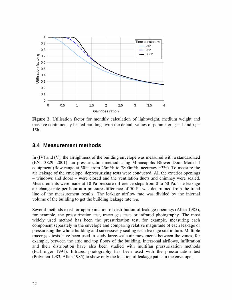
),(f τγ=η . (13) The average European values for the parameters were determined to be a0 = 1 and τ0 = 16h for the standard EN 832 and, later, for the monthly method of standard EN ISO 13790, the values were concluded to be a0 = 1 and τ0 = 15h for continuously heated buildings. The effect of thermal inertia of building structures on the utilisation factor is shown in Figure 3 with the default values of parameters a0 and τ0.

22

0

0.1

0.2

0.3

0.4

0.5

0.6

0.7

0.8

0.9

1

0 0.5 1 1.5 2 2.5 3 3.5 4

Gain/loss ratio γ

Util

isat

ion

fact

or η

Time constant τ: 24h 96h 336h

Figure 3. Utilisation factor for monthly calculation of lightweight, medium weight and massive continuously heated buildings with the default values of parameter a0 = 1 and τ0 = 15h.

3.4 Measurement methods In (IV) and (V), the airtightness of the building envelope was measured with a standardized (EN 13829: 2001) fan pressurization method using Minneapolis Blower Door Model 4 equipment (flow range at 50Pa from 25m³/h to 7800m³/h, accuracy ±3%). To measure the air leakage of the envelope, depressurizing tests were conducted. All the exterior openings – windows and doors – were closed and the ventilation ducts and chimney were sealed. Measurements were made at 10 Pa pressure difference steps from 0 to 60 Pa. The leakage air change rate per hour at a pressure difference of 50 Pa was determined from the trend line of the measurement results. The leakage airflow rate was divided by the internal volume of the building to get the building leakage rate n50. Several methods exist for approximation of distribution of leakage openings (Allen 1985), for example, the pressurization test, tracer gas tests or infrared photography. The most widely used method has been the pressurization test, for example, measuring each component separately in the envelope and comparing relative magnitude of each leakage or pressurising the whole building and successively sealing each leakage site in turn. Multiple tracer gas tests have been used to study large-scale air movements between the zones, for example, between the attic and top floors of the building. Interzonal airflows, infiltration and their distribution have also been studied with multifan pressurization methods (Fürbringer 1991). Infrared photography has been used with the pressurization test (Polvinen 1983, Allen 1985) to show only the location of leakage paths in the envelope.

23

It has been shown, for example in Allen (1985), that leakage distribution is a function of pressure difference over the envelope, due to the nonlinearity of leakage airflow rate over the pressure difference. Normally, there is a variety of cracks in the envelope with different values of flow exponent (see Equation 6), giving rise to a variation in leakage distribution, depending on the pressure difference. The difference can be substantial; for example, Warren (1980) reported up to 27 percentage units difference in leakage distribution over the envelope when the pressure difference was increased from 5Pa to 50Pa. The leakage distribution was studied in (IV) with a thermography test with pressurization, but the variation of flow exponent was not studied. A two-phase thermography test was used in (IV) to determine air leakage places and to approximate the area of the envelope (see Equation 4) that is affected by infiltration or exfiltration in (V). Also a method to approximate the distribution of infiltrating air based on the results of this kind of thermography test was developed. The thermography test was carried out with a FLIR ThermaCam P65 infrared image camera (thermal sensitivity of 0.08 °C, measurement range -40 °C to +500 °C) in the study. The test was performed inside the building during the heating season when the difference between the indoor and outdoor temperatures was 25°C. General requirements for the test conditions for the thermography of the building are given; for example, the minimum internal-to-external temperature difference during the test is 10°C according to the standard (EN 13187: 2001) or 15°C according to the guideline (LVI 10-10393: 2005). All external walls and the roof were investigated from inside the house. Thermography investigations were performed twice, see Figure 4. First, to determine the normal situation, the surface temperature measurements were performed without any additional air pressure difference. Next, to determine the main air leakage places, a 50 Pa negative pressure over the envelope was set with fan pressurization equipment. After the infiltration airflow had cooled the inner surface of the envelope, the surface temperatures were measured with the infrared image camera from the inside of the house. The temperature difference between these two measurements shows the air leakage. The relative decrease in the surface temperature was used to determine and to classify the air leakage places. The relative decrease in the surface temperature shows the relation of the temperature difference between the internal surface of the building envelope measured before and after the depressurization to the difference between the indoor and the outdoor air temperatures as follows

%100TTTT

Toutin

2i,s1i,s ⋅−

−=Δ , (14)

where ΔT is relative decrease in surface temperature (%), Ts,i1 is surface temperature of point i measured at the normal pressure conditions (°C), is Ts,i2 is surface temperature of point i measured at -50 Pa pressure conditions (°C), Tin is indoor air temperature (°C) and Tout is outdoor air temperature (°C).

24

a)

Surface temperatures before the depressurization Point Ts,i1, °C Sp1 17.9 Sp2 17.9 Sp3 18.7 Sp4 15.3

b)

Surface temperatures after the depressurization and relative temperature decrease Point Ts,i2, °C ΔT, % Sp1 13.2 19 Sp2 16.3 6 Sp3 15.6 12 Sp4 14.0 5

Figure 4. An example of infrared camera illustrations under normal (a) and -50 Pa pressure conditions (b). For the simulation model in (IV), the leakage routes of the modelling object were roughly classified according to the relative temperature decrease and the position. The shape or area of the leakage openings shown by the infrared camera illustrations are not taken into account, and nor are those leakage routes with a relative temperature decrease of less than 10%. The leakage routes that were taken into consideration were divided into three categories according to the relative temperature decrease ΔT, see Table 2. The temperature decrease was simply taken into account using the assumed weighting factors g of the categories. Because the relative temperature decrease is not absolute characteristic of air leakage (Kalamees et al. 2007), these weighting factors can not be defined accurately.

25

Table 2. Three categories of leakage routes based on the relative temperature decrease. The number x corresponds to the total number of leakage openings in the house that belong to these categories.

ΔT, % Weighting factor g Number x 10-20 1 33 20-30 2 18 >30% 3 5

The vertical position of the leakage routes was taken into account using five categories; see Table 3. Horizontally, the exact position of the leakage routes in an exterior wall was not taken into account; only the distribution of the leakage places between the facades was considered. This means that only one leakage opening per facade at any particular vertical position may exist in a zone. Table 3. Typical vertical positions of the air leakage openings on both floors of the detached house that was studied in (IV) and (V).

Category Z Typical place of the air leakage opening 1 Junction of external wall and roof 2 Upper edge of window frame 3 Lower edge of window frame 4 Junction of external wall and intermediate

floor 5 Junction of external wall and base floor.

53

2

34

2

4

1

The product G of the weighting factor g and number x of the leakage routes was calculated for each facade F and category Z as follows

Z,FZ,FZ,F xgG ⋅= . (15) The total sum of GF,Z in the house is calculated as the sum over all the facades F and the vertical positions Z

∑∑= =

=4

1F

5

1ZZ,F

tot GG . (16)

The distribution of the leakage openings in the house is approximated by dividing GF,Z by Equation (16)

%100GG

D totZ,F

Z.F ⋅= , (17)

26

where DF,Z is a proportion of a single leakage opening in the model to all the leakage openings taken into account. In (IV), the follow-up measurement of air pressure differences over the building envelope (see Figure 5) and air temperature inside and outside the building were conducted. Pressure differences were measured using calibrated FCO44 differential pressure transducers made by Furness Controls Ltd. The accuracy of these devices is better than ±2.5% in the measurement range from 0Pa to ±20Pa. Indoor and outdoor air temperatures were measured using Tinytag Plus loggers made by Gemini Data Loggers Ltd; the accuracy of this sensor is ±0.2°C in the range from 0°C to 50°C. Pressure difference and temperature data were collected using a 5-minute time step.

4.3m

2.5m

2 .6m

ΔP1

ΔP2

Figure 5. Measurement points of the air pressure difference over the building envelope on the base and the top floor of the house in (IV).

27

4 RESULTS

4.1 Balanced ventilation system The performance of various mechanical ventilation systems in apartment building was studied in (I) using IDA-ICE simulation tool. Results and description of the simulated cases are summarized in Table 4. The performance of a basic centralised constant air volume (CAV) mechanical supply and exhaust ventilation system was compared with a more flexible decentralised air handling system that had an option for variable air volume (VAV) suitable for demand-controlled ventilation with different control strategies. A centralised VAV ventilation system was considered to be too complicated and expensive for residential apartment buildings and was not studied. In the case of centralised ventilation systems, district heat was used to reheat the supply air (marked with “water”). Two levels of ventilation S2 and S3 were studied. The Class S2 rate of 8 l/s of fresh air per person is based on the Finnish classification of indoor climate (FiSIAQ 2001) for a high quality level of ventilation. Class S3 represents a lower level of ventilation, and agrees with the minimum requirements of the Finnish building code, i.e. 6 l/s per person and at least 0.5 ach. Table 4. Description of simulated cases and annual energy use in the simulated cases divided by net floor area of the apartment.

Case Description of the cases Results Number Air handling unit Mecha- Specific consumption, kWh/m²,a Recove-flats per- Centra- Sys- VAV Reheat Heat De- nical District heating Electricity Total red

sons lized: tem control coil reco- sign cooling Radi- Do- Venti- Coo- Fans House- energy, 'C' stra- very, air ators mes- lation ling and hold kWh/m²,adecent- tegy % flow and tic pumps electicityralized: venti- hot'D' lation water

Central 1 2 6 C CAV - water 60 S2 - 52.8 63.7 - - 5.4 34.9 156.7 63.1Central 2 1 3 C CAV - water 60 S2 - 49.9 63.7 - - 5.4 34.9 153.8 63.2Central 2S3 1 3 C CAV - water 60 S3 - 43.7 63.7 - - 4.4 34.9 146.7 51.4Central 2p2 1 2 C CAV - water 60 S2 - 53.5 63.7 - - 5.4 34.9 157.5 63.0Central 5 1 3 C CAV - water 60 S2 LR¹ 50.2 63.7 - 7.5 5.4 34.9 161.7 63.2Central 5a 1 3 C CAV - water 60 S2 LR¹ 50.4 63.7 - 9.5 5.4 34.9 163.9 63.2Central 6 1 3 C CAV - water 60 S2 LR¹, BR1² 50.4 63.7 - 7.6 5.4 34.9 161.9 63.2Local 1 1 3 D CAV - electricity 80 S2 - 26.5 63.7 5.5 - 11.2 34.9 141.7 94.4Local 1a 1 3 D CAV - electricity 60 S2 - 26.6 63.7 23.4 - 11.2 34.9 159.8 63.2Local 2 1 3 D CAV - - 80 S2 - 31.8 63.7 - - 11.1 34.9 141.6 94.4Local 3 1 3 D VAV CO2,T electricity 60 S2 - 22.7 63.7 11.8 - 8.2 34.9 141.3 38.2Local 4 1 3 D VAV CO2,T - 80 S2 - 25.3 63.7 - - 8.2 34.9 132.1 58.9Local 5 1 3 D VAV CO2 electricity 60 S2 - 22.4 63.7 11.3 - 5.7 34.9 137.9 32.7¹ Living room² Bedroom 1

28

Simulation Central 2 is used as a reference case since this example represents the most basic possible centralised ventilation system. In the studied cases (see Table 4), decentralisation of the ventilation system increased electricity use from 2.9 to 29 kWh/m²a compared to the Central 2 case, but total energy use of the apartment can be decreased up to 21.7 kWh/m² by means of higher efficiency of heat recovery and demand-controlled ventilation that were available with the decentralized ventilation system. The combination of VAV control with 80% heat recovery resulted in the lowest total energy consumption, which is illustrated by Local 4. The effect of VAV control with heat recovery efficiency of 60% can be seen by comparing the results of simulations Local 1a and Local 3. By comparing these cases, it can be seen that VAV control reduces total energy consumption by 18.5 kWh/m²a, and electrical energy consumption by 14.6 kWh/m²a. In the case of CO2 control only (Local 5), the savings are slightly higher, but this case is not comparable because of significantly reduced thermal comfort. When the heat recovery efficiency was 80%, the VAV control decrease total energy consumption by 9.6 kWh/m²a, which can be seen by comparing the results of Local 1 and Local 4. The effect of VAV control on energy use depends also on airflow rates and the set points of control that were used. The difference in energy consumption between Local 1 and Local 1a shows the results of a change of heat recovery efficiency from 60% to 80%. At 60% efficiency, the total energy consumption was 18.1 kWh/m²a higher than for 80% efficiency. Decreasing the air change rate from 0.85 ach to 0.69 ach reduces total energy consumption by 7.1 kWh/m²a (Central 2 vs. Central 2S3). The electrical load for mechanical cooling was between 7.5 to 9.5 kWh/m²a, being equivalent to19–24% of the total electricity consumption in the basic case, Central 2.

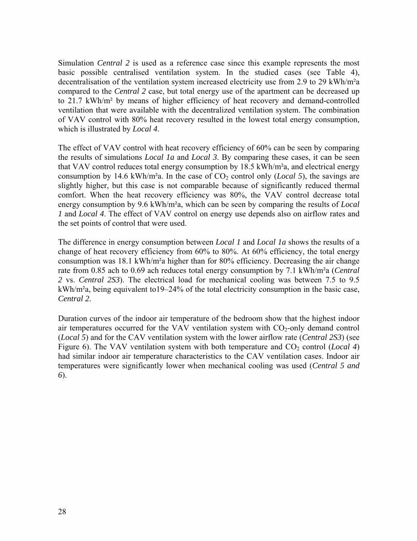
Duration curves of the indoor air temperature of the bedroom show that the highest indoor air temperatures occurred for the VAV ventilation system with CO2-only demand control (Local 5) and for the CAV ventilation system with the lower airflow rate (Central 2S3) (see Figure 6). The VAV ventilation system with both temperature and CO2 control (Local 4) had similar indoor air temperature characteristics to the CAV ventilation cases. Indoor air temperatures were significantly lower when mechanical cooling was used (Central 5 and 6).

29

20

22

24

26

28

30

32

34

36

38

0 10 20 30 40 50 60 70 80 90 100Time, %

Tem

pera

ture

, °C

Local 5

Central 2S3

Central 2, Local 4

Central 5

Central 6

Figure 6. Duration curves of air temperature of the bedroom during one year. Mechanical cooling of the apartment was required for less than 34% of the year. Peak powers of the cooling cases are shown in Table 5, where a peak power of 100% is defined as the maximum cooling power required at any instant during the year. In the simulated cases, the 99.9 percentile is between 83 and 85% of the peak power of 100%. This represents the ninth highest value of cooling power during the year. In the studied cases, the range of peak powers divided by the net floor area of the apartment, are 22-24 W/m² (100%) and 18-20W/m² (99.9%). Table 5. Peak cooling power of the air conditioners. Powers of the table are sensible powers that were simulated with venetian blinds.

4.2 Electrically heated windows The efficiency of electrically heated windows and U-value were studied in (II) using a numerical RC-network model. The U-value is commonly used to describe conduction losses in building envelope parts, i.e., for wall structures without internal heat gains. In such walls, heat flux is constant (in the steady state) in every layer. In a heated window, electrical heating power is switched to the selective layer of the pane. This means that the heat fluxes in the inner and outer panes are not equal and have commonly reverse directions. Thus, the U-value which has physical meaning is to be defined based on the heat flux from the outer surface to outdoors. It should be noticed that the U-value stated for the inner surface would have a negative value. The U-value of an unheated or a heated window is expressed as

Case Peak power (99.9%), W Peak power (100%), WBR1 Living room Total BR1 Living room Total

Central 5 - 1 428 1 428 - 1 717 1 717Central 5a - 1 546 1 546 - 1 817 1 817Central 6 337 1 201 1 538 451 1 403 1 854

30

outin

offoutoff

TTq

U−

= , outin

onouton

TTq

U−

= , (18)

where q is heat flux (W/m2), subscript out refers to the direction of heat flux (from outer surface to outdoors) and superscript off to an unheated window (a common window or heated window switched off) and on to a heated window and Tin – Tout is the difference between the indoor and outdoor temperatures. The efficiency of windows can be derived by comparing two different heating setups which are shown in Figure 7. In Figure 7, the heated window is combined with convective heating where heat is introduced directly into the air volume. In the first setup in Figure 7(a), there is convective heating only and in the second setup in Figure 7(b), in addition, the window is heated. The heat loss through the walls is set to zero (q = 0W/m²) and because this term is the same in both setups, it will be cancelled out in the derivation of efficiency.

Chamber wall

offoutq

Window

²m/W0q =

offQ

a)

onoutqon

inqonQ

²m/W0q =

P

b)

Figure 7. Derivation the efficiency by comparing the additional heat loss caused by electrical heating of the window to case with convective heating and unheated window. (a) A fully convective heating (Qoff) where convective heat is introduced directly into air. (b) Heated window and positive or negative convective heat output (Qon) for maintaining the same indoor air temperature as in (a). The efficiency of electrically heated windows, which may be used for improving thermal comfort near glazing, can be expressed as the difference between the convective heat terms needed to maintain the same indoor temperature in relation to the electrical heat output of the window

pQQ onoff −

=ϕ , (19)

where ϕ is efficiency of heated windows (-), Q is convective heat introduced into air (W), superscript off refers to the unheated window and on to the heated window and p is heat output of the window (W). Expanding the terms in Equation (19) by substituting the heat balance of indoor air and the heated window, see Figure 7, the efficiency can be expressed as

31

Pqq

1P

qq offout

onout

onin

offout −

−=+

=ϕ , (20)

where subscript in refers to the direction of heat flux (from inner surface to indoors) and P is electrical heat output of the window (W/m²). The first expression in Equation (20) gives useful formulation: efficiency is the proportion of the electrical heat output P, which is used to cover the heat losses of the window and for the heating of the room. The second form of Equation (20) can be stated directly, based on an additional heat loss in the heated window: the efficiency is equal to 1 minus the additional heat loss in relation to the electrical heat output. The RC-model of the electrically heated windows was completed and the efficiency of several window types was calculated numerically. The effect of the temperature of the inner surface on the efficiency is shown in Figure 8 for a double-glazed window with three surface temperatures. This window has a selective layer with emission factor εw = 0.2 and the U-value is within the range from 1.97 to 1.73 W/m2⋅K at an outdoor temperature of –20 to +10 ºC, respectively. The indoor temperature is 20 ºC. Figure 8 shows a significant outdoor temperature dependency for the efficiency compared to the surface temperature dependency, because the effect of the surface temperature is less than one percentage unit in efficiency.

0.64

0.65

0.66

0.67

0.68

0.69

0.70

0.71

-20 -15 -10 -5 0 5 10Outdoor air temperature, °C

Effic

ienc

y, -

T1 = 30 °CT1 = 25 °CT1 = 20 °C

Double-glazing, AirP = 25…230 W/m2

T1 = 30 °CT1 = 25 °CT1 = 20 °C

Figure 8. The dependency of the efficiency on outdoor air temperature and inner surface temperature (T1) in the case of a double-glazed window with U-value of 1.8 W/m2⋅K at rating conditions. Heat output to the room as a function of temperature difference between surface and indoor air is shown in Table 6 in the case of free convection on the inner surface without any

32

disturbance caused by indoor airflows (Incropera and De Witt 1990), which is assumed to be valid for radiant floor heating. Table 6. Heat output to the room from electrically heated windowpane.

Temperature difference (surface – indoor), °C 0 5 10 20 Heat flux to the room, W/m² 0 32.8 72.0 162.0

The effect of heat transfer between inner windowpane and room air on efficiency of the windows was studied with two different convective heat transfer relations: the relation for free convection (Incropera and DeWitt 1990) and the relation developed for window surface with radiator heating (Khalifa and Marshall 1990). The following values are given at –10 ºC outdoor air temperature and 25 ºC surface temperature:

- glazing-Double K)10.2W/m²2.5h( %73%65 c ⋅→=→=ϕ

- glazing.-Triple K)9.2W/m²2.2h( %84%76 c ⋅→=→=ϕ The efficiency and U-values at varying outdoor temperature are shown in Figure 9 for two window types at 25 ºC inner surface temperature. The U-value of unheated double-glazed windowpanes is 1.1 W/m²⋅K at rating conditions (outdoor temperature 0°C) and triple-glazed window 0.5 W/m²⋅K, respectively. The efficiency of highly insulated triple-glazed windows is about 10 percentage units higher and the dependency on outdoor air temperature is slightly lower compared to double-glazed windows. Figure 9 shows that the variation of the efficiency of the triple- and double-gazed windows are 3 and 5 percentage units when the outdoor temperature ranges from -20 to +10°C. In Figure 9 the outdoor temperature dependency of U-values is result from non-linearity in the convective and radiation heat transfer between the windowpanes. In the case of heated window, U-value is also dependent on electrical heat output P as shown in Equation (18) and Figure 7.

33

0.76

0.77

0.78

0.79

0.80

0.81

0.82

-20 -15 -10 -5 0 5 10Outdoor air temperature, °C

Effic

ienc

y, -

0.75

1.00

1.25

1.50

1.75

2.00

2.25

U-v

alue

from

out

er s

urfa

ce, W

/m2 K

Efficiency, -Uoff, W/m2KUon, W/m2K

Double-glazing KryptonT1 = 25 °C

Uoff, W/m2KUon, W/m2K

a)

0.87

0.88

0.89

0.90

0.91

0.92

-20 -15 -10 -5 0 5 10Outdoor air temperature, °C

Effic

ienc

y, -

0.40

0.50

0.60

0.70

0.80

0.90

U-v

alue

from

out

er s

urfa

ce, W

/m2 K

Efficiency, -Uoff, W/m2KUon, W/m2K

Triple-glazing(2X low ε=0,04) KryptonT1 = 25 °C

Uoff, W/m2KUon, W/m2K

b)

Figure 9. The efficiency and U-values for double-glazed (a) and highly insulated triple-glazed windows (b). The double-glazed window has one low-emission (εw = 0.04) selective layer and the triple-glazed two layers. When efficiencies of all the studied windows shown in (II) were plotted against the U-value of an unheated window, the linear correlation shown in Figure 10 can be drawn. In Figure 10 the efficiencies and U-values were plotted for studied outdoor temperatures (-20, -10, 0 and +10°C) and for inner windowpane surface temperatures (20 and 25°C). The efficiency is slightly outdoor temperature dependent because of the outdoor temperature dependency of U-values, as shown in Figure 9, but the correlation shows in Figure 10, that efficiency is primarily dependent on the U-value of an unheated window.

34

y = -0.175x + 0.985R2 = 0.984

0.6

0.7

0.8

0.9

1.0

0.0 0.5 1.0 1.5 2.0

U-value, W/m2K

Effic

ienc

y, -

T1 = 25 °CT1 = 20 °CLinear (T1 = 25 °C)

T1 = 25 ºCT1 = 20 ºC Linear (T1 = 25 ºC)

Figure 10. The efficiencies of double- and triple-glazed windows filled with air and krypton plotted against U-value of unheated window at +10 ºC, 0 ºC, –10 ºC and –20ºC outdoor temperatures and at 25ºC and 20 ºC inner pane surface temperatures (T1). The outdoor temperature dependency of the U-value explains why the same window shows different values of efficiency at different outdoor temperatures in Figure 10. According to Figure 10, efficiency can be expressed by the following linear equation

U175.0985.0 ⋅−=ϕ , (21)

where U is the U-value of an unheated window at a specific outdoor temperature (W/m²⋅K). The linear correlation shows an error of 0.015 at U = 0 as efficiency should be 1 at U = 0. Equation (21) applies for any outdoor air temperature within the range from -20°C to +10°C due to outdoor-temperature-dependent U-value. If a U-value is known only at rating conditions, the efficiency is obtained at rating conditions and the variation caused by the outdoor-temperature dependency of the U-value cannot be estimated. It was also shown in (II) that efficiency formulas may be further simplified for a given window-type by the use of constant heat transfer coefficients; efficiency was expressed as a function of outdoor temperature only ϕ = f(Tout). The error caused by simplification was less than 2.3% within the outdoor-temperature range from -20°C to +10°C.

35

4.3 Calibration of EN ISO 13790 The calibration of EN ISO 13790 against IDA-ICE was conducted in (III) with 30 different cases, including apartment buildings, detached houses and office buildings. The cases were selected to include the typical variety of building factors: thermal inertia of building structures and level of thermal insulation. The effect of internal and solar heat gains was also studied. The structures of the studied buildings were lightweight steel or wood frame constructions in the lightweight cases. In the medium weight cases, all the walls were lightweight, but there was a concrete intermediate floor in the apartment and the office buildings and a concrete base floor in the detached house. The roof of the detached house was lightweight. In the massive cases, all the structures of the buildings were massive concrete structures. Only the interior walls of the office building were lightweight. The time constant of the buildings calculated according to EN ISO 13790 was 16-41h in the lightweight cases, 56-200h in the medium weight cases and 223-439h in the massive cases. Two levels of internal heat gains were studied: Finnish internal heat gains, which were considered to be typical in Finland, and CEN heat gains defined by standard EN ISO 13790. The annual sum of CEN heat gains were about 20-50% lower than the Finnish heat gains, depending on the building type. Two levels of thermal insulation were also studied: the basic, when U-values correspond to the minimum requirements of the Finnish building code C3 (2003), for example 0.25W/m²⋅K for external walls or 1.4 W/m²⋅K for windows, or they are slightly better. At the improved level, U-value for the external wall is 0.19 W/m²K and 0.8-1.0 W/m²⋅K for the windows, respectively.

4.3.1 Selection of a0 and τ0 The procedure for selecting the parameters in (III) was based on the effect of thermal inertia of the building structures on heat demand and the difference in heat demand between IDA-ICE and EN ISO 13790. The effect of thermal inertia m between the lightweight and massive cases was calculated by

%100Q

QQm LW

ah

Mah

LWah ⋅⎟⎟

⎠

⎞⎜⎜⎝

⎛ −= , (22)

where Qah is annual heat demand of the building (kWh/m²a), superscript LW refers to the lightweight building and M to the building with massive structures. The parameters of EN ISO 13790 were determined for every studied building type so that the effect of thermal inertia on annual heat demand (Equation 22) corresponds to the results of IDA-ICE in Finnish conditions as closely as possible. Furthermore, the average difference e in annual

36

heat demand between the dynamic simulation and EN ISO 13790 should reach the smallest possible value

∑= −

−− −⋅=

y

1kk

IDAah

kENah

kIDAah

Q

QQ%100

y1e , (23)

where y is the number of cases, Qah-IDA is annual heat demand calculated with IDA-ICE (kWh/m²a) and Qah-EN is annual heat demand calculated with EN ISO 13790 (kWh/m²a). Every building type was studied with 480 combinations of a0 and τ0. Suitable parameters for Finnish conditions were chosen with the intersectional points shown in Figure 11.

a) b)

c)

Figure 11. The effect of thermal inertia on heat demand of the apartment building (a), office building (b) and (c) detached house according to IDA-ICE (dotted line) and EN ISO 13790. The combinations of the studied a0 and τ0 closest to the intersectional points for the apartment and office buildings are listed in Table 7. For the apartment building, the most suitable parameters are (a0 = 6, τ0 = 7h). For the office building, the selected parameters were (a0 = 2, τ0 = 15h), even if the difference between the methods is unacceptably high. For the detached house, EN ISO 13790 indicates a higher effect of thermal inertia than

0

2

4

6

8

10

12

14

16

18

20

0 1 2 3 4 5 6 7 8 9 10 11 12 13 14 15 16 17 18 19 20τ0, h

m, %

= 0.1 = 0.5 = 1 = 2 = 3 = 4 = 5 = 6

IDA-ICE: 9.3%

a0

a0

a0

a0

a0

a0

a0

a0

0

4

8

12

16

20

24

28

32

36

40

0 1 2 3 4 5 6 7 8 9 10 11 12 13 14 15 16 17 18 19 20τ0, h

m, %

= 0.1 = 0.5 = 1 = 2 = 3 = 4 = 5 = 6

IDA-ICE: 29.8%a0

a0

a0 a0

a0 a0

a0 a0

10

12

14

16

18

20

22

24

26

28

30

0 1 2 3 4 5 6 7 8 9 10 11 12 13 14 15 16 17 18 19 20

τ0, h

m, %

= 0.1 = 0.5 = 1 = 2 = 3 = 4 = 5 = 6

IDA-ICE: 15.1%

a0

a0

a0

a0

a0

a0

a0

a0

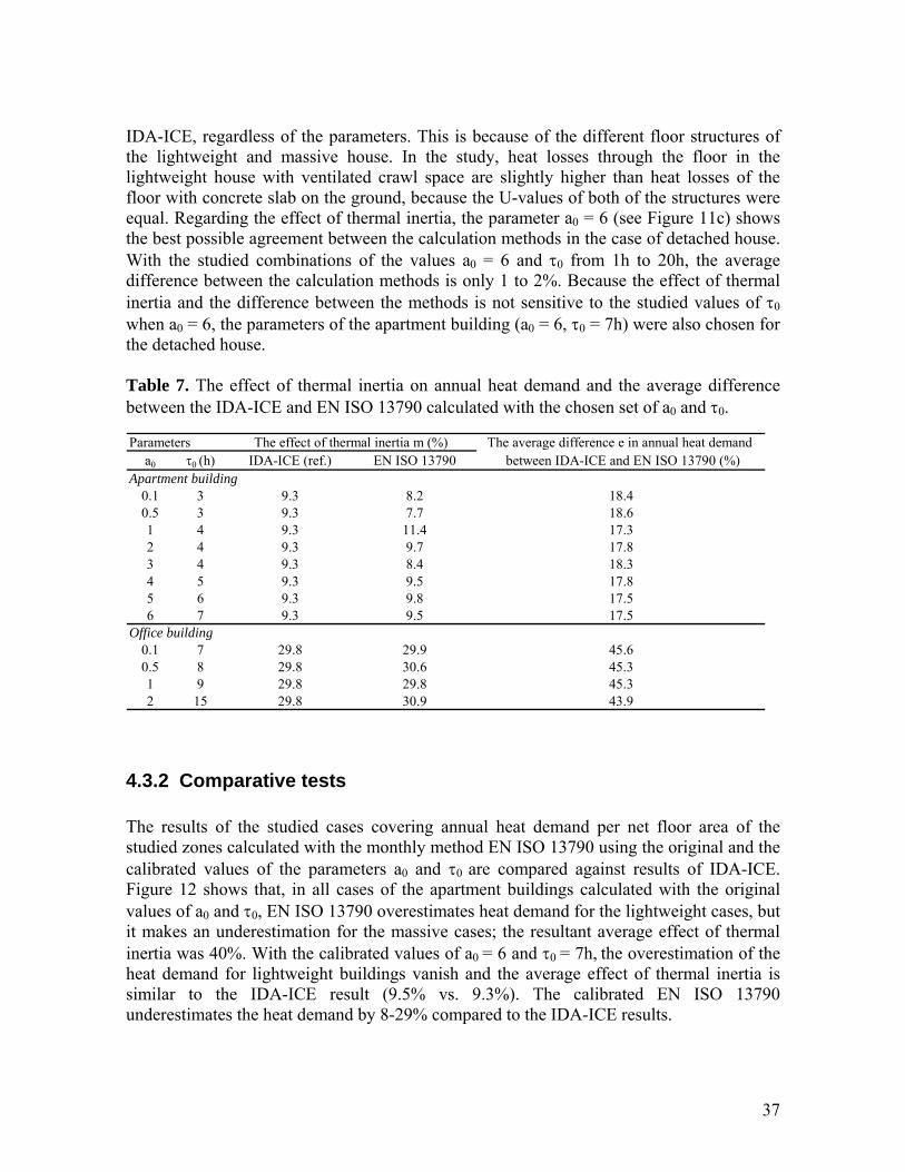
37

IDA-ICE, regardless of the parameters. This is because of the different floor structures of the lightweight and massive house. In the study, heat losses through the floor in the lightweight house with ventilated crawl space are slightly higher than heat losses of the floor with concrete slab on the ground, because the U-values of both of the structures were equal. Regarding the effect of thermal inertia, the parameter a0 = 6 (see Figure 11c) shows the best possible agreement between the calculation methods in the case of detached house. With the studied combinations of the values a0 = 6 and τ0 from 1h to 20h, the average difference between the calculation methods is only 1 to 2%. Because the effect of thermal inertia and the difference between the methods is not sensitive to the studied values of τ0 when a0 = 6, the parameters of the apartment building (a0 = 6, τ0 = 7h) were also chosen for the detached house. Table 7. The effect of thermal inertia on annual heat demand and the average difference between the IDA-ICE and EN ISO 13790 calculated with the chosen set of a0 and τ0.

4.3.2 Comparative tests The results of the studied cases covering annual heat demand per net floor area of the studied zones calculated with the monthly method EN ISO 13790 using the original and the calibrated values of the parameters a0 and τ0 are compared against results of IDA-ICE. Figure 12 shows that, in all cases of the apartment buildings calculated with the original values of a0 and τ0, EN ISO 13790 overestimates heat demand for the lightweight cases, but it makes an underestimation for the massive cases; the resultant average effect of thermal inertia was 40%. With the calibrated values of a0 = 6 and τ0 = 7h, the overestimation of the heat demand for lightweight buildings vanish and the average effect of thermal inertia is similar to the IDA-ICE result (9.5% vs. 9.3%). The calibrated EN ISO 13790 underestimates the heat demand by 8-29% compared to the IDA-ICE results.

Parameters The effect of thermal inertia m (%) The average difference e in annual heat demand a0 τ0 (h) IDA-ICE (ref.) EN ISO 13790 between IDA-ICE and EN ISO 13790 (%)

Apartment building0.1 3 9.3 8.2 18.40.5 3 9.3 7.7 18.61 4 9.3 11.4 17.32 4 9.3 9.7 17.83 4 9.3 8.4 18.34 5 9.3 9.5 17.85 6 9.3 9.8 17.56 7 9.3 9.5 17.5

Office building0.1 7 29.8 29.9 45.60.5 8 29.8 30.6 45.31 9 29.8 29.8 45.32 15 29.8 30.9 43.9

38

Figure 12. Annual heat demand of the apartment building calculated with IDA-ICE and EN ISO 13790. The agreement between EN ISO 13790 and IDA-ICE is better with the detached house (see Figure 13). The original EN ISO 13790 shows good agreement with the IDA-ICE results for the massive and medium-weight cases. But, as with the apartment building, EN ISO 13790 overestimates the effect of thermal inertia; the resultant average effect of thermal inertia was 25%. With the calibrated values, the overestimation of the heat demand for the lightweight building is reduced and the effect of thermal inertia is closer to the IDA-ICE results (18.3% vs. 15.1%) and the difference between the results of the calculation methods is 0-9%.

0

5

10

15

20

25

30

35

Light Medium Massive Light Medium Massive Light Medium Massive Light Medium Massive

Hea

t dem

and,

kW

h/m

²a

(Finnish heat gains) (CEN heat gains) (Improved thermal insulation) (SP windows)

100%100% 100%

100% 100%

100%

100% 100% 100%

100% 100% 100%

137%

102%

92%

105%

94% 91%

146%

73%

134%

94% 81%

91%

IDA-ICE EN ISO 13790 (a0=1, τ0=15h) EN ISO 13790 (a0=6, τ0=7h)

87% 87% 92%

87%88% 90%

76%71% 71%

82%79% 80%

39

Figure 13. Annual heat demand of the detached house calculated with IDA-ICE and EN ISO 13790. Heat demand in the office building is strongly underestimated for all the building structures regardless of the values of a0 and τ0 (see Figure 14). At the same time, the resultant annual heat losses of the methods are almost equal; they are only 1.5-2.4% lower, according to EN ISO 13790. The effect of thermal inertia could be corrected quite close to the IDA-ICE results (30.9% vs. 29.8%) with the modified values, but the use of the monthly method for office buildings in Finnish conditions is questionable due to the strong underestimation of heat demand.

0

10

20

30

40

50

60

70

80

90

100

Light Medium Massive Light Medium Massive Light Medium Massive

Hea

t dem

and,

kW

h/m

²a

(Finnish heat gains) (CEN heat gains) (Improved thermal insulation)

100%

100% 100%

100%

100% 100%

100%

100%

114%

105% 103%

113%

105% 103%

119%

103%

IDA-ICE EN ISO 13790 (a0=1, τ0=15h) EN ISO 13790 (a0=6, τ0=7h)104%

102% 102%

104%

102% 103%

109%

100% 100%100%

100%

40

Figure 14. Annual heat demand of the office building calculated with IDA-ICE and EN ISO 13790.

4.4 Infiltration of building envelope

4.4.1 Evaluation of the simulation model The evaluation of a multizone infiltration model of an existing two-storey detached house was performed in (IV) by comparing the simulated and measured pressure conditions of the building during a three-week test period in the heating season. Two different cases were simulated concerning the methods of defrost protection of the heat recovery system in the air handling unit:

• Case 1: On/off control of the supply fan, as it is in the measured house. • Case 2: Bypass control of the supply fan.

The differences in the average indoor air temperatures between the measurement and simulation results were 0.2°C or less during the test period and the differences between the average pressure differences were also quite small; the maximum error is 0.6Pa in case 1 and 1.1Pa in case 2, see Table 8. Figure 15 shows the measured and simulated hourly air pressure differences over the envelope. In both simulation cases, the model gives some peaks that clearly deviate from the measured pressure. For example, the measured peaks of pressure differences were positive on the top and base floors on 17th March, but the model gave opposite (negative) pressure differences. In case 1, the simulated pressure differences

0

5

10

15

20

25

30

35

40

Light Medium Massive Light Medium Massive Light Medium Massive

Hea

t dem

and,

kW

h/m

²a

(Finnish heat gains) (CEN heat gains) (Improved thermal insulation)

100%

100%100%

100%

100% 100% 100%

100% 100%

64%

55% 55%

75%

72% 72%

54%

42% 41%

IDA-ICE EN ISO 13790 (a0=1, τ0=15h) EN ISO 13790 (a0=2, τ0=15h)

55%

55% 55%

68%

72% 72%

46%

41% 41%

41

follow the measurement results more precisely and the correspondence between the results is quite good, while the model tends to overestimate the pressure differences more in case 2. Table 8. Measured and simulated average indoor air temperatures and pressure differences over the envelope during the three-week test period.

Indoor air temperature, °C Pressure difference, Pa Method 1st floor 2nd floor 1st floor 2nd floor

Measurement 19.7 17.0 -3.3 1.9 Simulation-case 1 19.7 17.2 -2.7 2.2 Simulation-case 2 19.8 17.2 -2.2 2.8

-8

-7-6

-5

-4

-3

-2

-1

0

1

2

5. 6. 7. 8. 9. 10. 11. 12. 13. 14. 15. 16. 17. 18. 19. 20. 21. 22. 23.

Date (day of March)

ΔP, P

a

1. floor (measurement)1. floor (simulation_case-1)1. floor (simulation_case-2)

a)

-3

-2

-1

0

1

2

3

4

5

6

5. 6. 7. 8. 9. 10. 11. 12. 13. 14. 15. 16. 17. 18. 19. 20. 21. 22. 23.Date (day of March)

ΔP,

Pa

2. floor (measurement)2. floor (simulation_case-1)2. floor (simulation_case 2)

b)

Figure 15. Measured and simulated air pressure conditions of the detached house on the base (a) and top (b) floors during the three-week measurement period from 5th to 24th March 2005. The air pressure differences are shown as a function of the temperature difference between indoor and outdoor air in Figure 16. According to the measurement results, the pressure difference decreases with an increasing temperature difference on the base floor, but the temperature dependence of the pressure difference is weak on the top floor. The different measured correlations between the air pressure and the temperature differences on the base and top floors are the result from the stack effect and the ventilation system. A need of defrost protection of the ventilation system increases in the measured house as the outdoor temperature decreases. The effect of defrost protection on air pressure distribution depends on ventilation air flow rates of each room types. Results show that the temperature dependence of the pressure difference can be simulated more accurately in case 1, where the defrost protection method of the modelling object is taken into account. In case 2, where the fans of the air handling unit are always on, the model predicts somewhat higher pressure differences than the measurement result at the lowest outdoor air temperatures.

42

-8-7-6-5-4-3-2-1012

10 15 20 25 30 35 40Temperature difference (Tin-Tout), °C

ΔP,

Pa

1. floor (measurement)1. floor (simulation-case1)Linear (measurement)Linear (simulation-case-1)

Measurement: R2 = 0.5917 Simulation: R2 =0.5183

a)

-8-7-6-5-4-3-2-1012

10 15 20 25 30 35 40Temperature difference (Tin-Tout), °C

ΔP,

Pa

1. floor (measurement)1. floor (simulation-case 2)Linear (measurement)Linear (simulation-case 2)

Measurement: R2 = 0.5917

Simulation: R2 = 0.2076

b)

-3

-2

-1

0

1

2

3

4

5

6

10 15 20 25 30 35 40Temperature difference (Tin-Tout), °C

ΔP,

Pa

2. floor (measurement)2. floor (simulation-case-1)Linear (measurement)Linear (simulation-case1)

Measurement: R2 = 0.0226

Simulation: R2 = 0.0274

c)

-3

-2

-1

0

1

2

3

4

5

6

10 15 20 25 30 35 40Temperature difference (Tin-Tout), °C

ΔP,

Pa

2. floor (measurement)2. floor (simulation-case 2)Linear (measurement)Linear (simulation-case 2)

Measurement: R2 = 0.0226

Simulation: R2 = 0.1633

d)

Figure 16. Measured and simulated pressure conditions of the detached house on the base (a, b) and top (c, d) floors during the test period. The pressure differences are shown as a function of the temperature difference between indoors and outdoors. The error, defined as the difference between the measured and simulated air pressure differences (case 1) over the envelope on the top floor, is shown as a function of local wind speed and direction (see Figure 17). In Figure 17(a) the local wind speed at the level of the roof of the detached house was approximated using a wind profile equation developed by Sherman and Grimsrud (1980) and the wind direction shown in Figure 17(b) is the measurement result from the weather station. This error between the measured and simulated air pressure differences does not depend on the wind speed and the mean absolute values of the error between the compass points give an indication that the error does not depend strongly on the wind direction.

43

R2 = 0.0001

-4

-3

-2

-1

0

1

2

3

4

0 1 2 3 4 5 6 7Wind speed, m/s

Erro

r, Pa

a)

-4

-3

-2

-1

0

1

2

3

4

0 90 180 270 360

Wind direction

Erro

r, Pa

North East South West North

-0.5Pa -0.5Pa 0.8Pa 0.9Pa

b)

Figure 17. The errors between the simulated (case 1) and measured air pressure differences over the envelope on the top floor. The errors are shown as a function of wind speed (a) and direction (b). The average errors between the main compass points are also shown (b).

4.4.2 Infiltration analyses In (I), infiltration of a seven-storey house was studied using IDA-ICE simulation tool in a single case with approximate initial data concerning airtightness and distribution of leakage paths and calculation of wind pressure. Two apartments and a staircase were simulated and the approximation of average infiltration rate of the building was concluded to be 0.05 ach in sheltered wind conditions. In (V), the effect of various factors on infiltration and heat energy use of Finnish detached houses were simulated with IDA-ICE using the evaluated model shown in (IV) and a simple adapted infiltration model was developed based on the simulation results. The cases were simulated with three levels of airtightness. Almost completely airtight detached houses were described with a building leakage rate of n50 = 0.15 ach, while the airtightness of typical detached houses was simulated using n50 = 3.9 ach; the leakage air change rate n50 = 10 ach describes leaky detached houses. According to extensive field measurements from 170 Finnish detached houses (Vinha et al. 2005, Korpi 2007), the mean value of n50 is 3.9 ach in timber frame houses, 5.8 ach in log houses and 2.3 ach in houses made of concrete, brick or lightweight block (see Figure 18). Because no clear correlation between flow exponent (n) and building leakage rate (n50) can be found in 170 measured Finnish detached houses, most of the studied cases in (V) were simulated with mean value of flow exponent 0.73. The effect of flow exponents was also studied with values 0.63 and 0.83. Over 90% of the measured flow exponents were in the range of 0.73 ± 0.1.

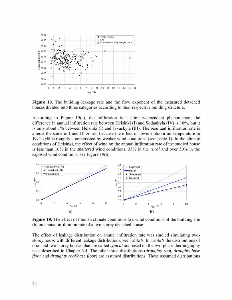
44

0.50

0.55

0.60

0.65

0.70

0.75

0.80

0.85

0.90

0.95

0 1 2 3 4 5 6 7 8 9 10 11 12 13 14 15 16n50, 1/h

Flow

exp

onen

t n,-

Timber frame Log Concrete/brick/lightweight block

Figure 18. The building leakage rate and the flow exponent of the measured detached houses divided into three categories according to their respective building structure. According to Figure 19(a), the infiltration is a climate-dependent phenomenon; the difference in annual infiltration rate between Helsinki (I) and Sodankylä (IV) is 10%, but it is only about 1% between Helsinki (I) and Jyväskylä (III). The resultant infiltration rate is almost the same in I and III zones, because the effect of lower outdoor air temperature in Jyväskylä is roughly compensated by weaker wind conditions (see Table 1). In the climate conditions of Helsinki, the effect of wind on the annual infiltration rate of the studied house is less than 10% in the sheltered wind conditions, 35% in the rural and over 50% in the exposed wind conditions, see Figure 19(b).

0.0

0.1

0.2

0.3

0.4

0 2 4 6 8 10n50, 1/h

n inf, a

ch

Sodankylä (IV)Jyväskylä (III)Helsinki (I)

a)

0.00.10.20.30.40.50.60.70.8

0 2 4 6 8 10n50, 1/h

n inf

, ach

ExposedRuralShelteredNo wind

b)

Figure 19. The effect of Finnish climate conditions (a), wind conditions of the building site (b) on annual infiltration rate of a two-storey detached house. The effect of leakage distribution on annual infiltration rate was studied simulating two-storey house with different leakage distributions, see Table 9. In Table 9 the distributions of one- and two-storey houses that are called typical are based on the two-phase thermography tests described in Chapter 3.4. The other three distributions (draughty roof, draughty base floor and draughty roof/base floor) are assumed distributions. These assumed distributions

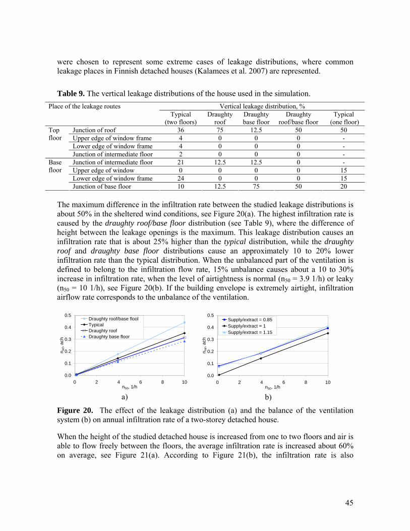
45

were chosen to represent some extreme cases of leakage distributions, where common leakage places in Finnish detached houses (Kalamees et al. 2007) are represented. Table 9. The vertical leakage distributions of the house used in the simulation.

Vertical leakage distribution, % Place of the leakage routes Typical

(two floors) Draughty

roof Draughty base floor

Draughty roof/base floor

Typical (one floor)

Junction of roof 36 75 12.5 50 50 Upper edge of window frame 4 0 0 0 - Lower edge of window frame 4 0 0 0 -

Top floor

Junction of intermediate floor 2 0 0 0 - Junction of intermediate floor 21 12.5 12.5 0 - Upper edge of window 0 0 0 0 15 Lower edge of window frame 24 0 0 0 15

Base floor

Junction of base floor 10 12.5 75 50 20 The maximum difference in the infiltration rate between the studied leakage distributions is about 50% in the sheltered wind conditions, see Figure 20(a). The highest infiltration rate is caused by the draughty roof/base floor distribution (see Table 9), where the difference of height between the leakage openings is the maximum. This leakage distribution causes an infiltration rate that is about 25% higher than the typical distribution, while the draughty roof and draughty base floor distributions cause an approximately 10 to 20% lower infiltration rate than the typical distribution. When the unbalanced part of the ventilation is defined to belong to the infiltration flow rate, 15% unbalance causes about a 10 to 30% increase in infiltration rate, when the level of airtightness is normal (n50 = 3.9 1/h) or leaky (n50 = 10 1/h), see Figure 20(b). If the building envelope is extremely airtight, infiltration airflow rate corresponds to the unbalance of the ventilation.

0.0

0.1

0.2

0.3

0.4

0.5

0 2 4 6 8 10n50, 1/h

n inf

, ach

Draughty roof/base floolTypicalDraughty roofDraughty base floor

a)

0.0

0.1

0.2

0.3

0.4

0.5

0 2 4 6 8 10n50, 1/h

n inf

, ach

Supply/extract = 0.85Supply/extract = 1Supply/extract = 1.15

b)

Figure 20. The effect of the leakage distribution (a) and the balance of the ventilation system (b) on annual infiltration rate of a two-storey detached house. When the height of the studied detached house is increased from one to two floors and air is able to flow freely between the floors, the average infiltration rate is increased about 60% on average, see Figure 21(a). According to Figure 21(b), the infiltration rate is also

46

increased by 36% when the flow exponent 0.73 is reduced by 0.1; it is decreased respectively by 27% if the flow exponent is increased by the same amount.

0.0

0.1

0.2

0.3

0.4

0 2 4 6 8 10n50, 1/h

n inf

, ach

2 floors1 floor

a)

0.0

0.1

0.2

0.3

0.4

0.5

0 2 4 6 8 10n50, 1/h

n inf

, ach

n = 0.63n = 0.73n = 0.83

b)

Figure 21. The effect of the height of the building (a) and the flow exponent (b) on annual infiltration rate of a two-storey detached house. If the average annual infiltration air change rate is used in the heat energy calculation, the outdoor air temperature dependence of infiltration airflows should be taken into account in the cold climate. This can be taken into account by, for example, calculating the annual infiltration air change weighted by the temperature difference of the indoor and outdoor air

∑

∑

=

=−

−

⋅−= 8760

1ii

ioutin

8760

1i

iinfi

ioutin

einf

)TT(

n)TT(n , (24)

where ninf-e is the average annual infiltration air change rate suitable for heat energy calculation (ach), ni

inf is normal hourly infiltration air change rate (ach), Tin is a set point temperature of heating (°C) and Ti

out is hourly outdoor air temperature (°C). This temperature correction could also be performed dividing the annual infiltration rate by a correction factor, which depends to some extent on the wind conditions being 0.86 in the sheltered wind conditions, 0.93 in the rural or 0.97 in the exposed, according to the IDA-ICE simulation results. The climate dependence of the factor is insignificant in Finland. A rough approximation of this correction factor can be considered to be 0.9 in the sheltered and moderate (rural) wind conditions.

4.4.3 The adapted infiltration model The average infiltration rate correlates almost linearly with the building leakage rate in most of the cases shown in Chapter 4.4.2. Because of this the infiltration rate can be roughly approximated by the widely used relation dividing the building leakage rate n50 by a case-dependent denominator x

47

xn

n 50inf = . (25)

The effect of the studied factors on the denominator x can be simply taken into account using the numerical results shown in Chapter 4.4.2. Instead of deriving the average constant denominator for Finnish detached houses, the effect of the studied factors can be taken into account by using, for example, a simple adapted model expressing the denominator as a product of several correction factors, using the principle shown in Sherman (1987)

BEHDWLn

n 50inf ⋅⋅⋅⋅⋅

= , (26)

where L is a climate-dependent factor, W is a factor for the wind conditions, D is a factor for leakage distribution, H is a factor for house height, E is a factor for the flow exponent and B is a factor for the balance of the mechanical supply and exhaust ventilation system. The values of the correction factors determined from the sensitivity analysis are listed in Table 10. The annual infiltration rate of Finnish detached houses can be estimated substituting these correction factors into Equation (26). Table 10. Correction factors for the adapted model.

Climate zone I-III IV L 27 25

Wind conditions exposed rural sheltered W 0.5 0.7 1

Leakage distribution dr. roof/base floor typical dr. roof dr. base floor D 0.8 1 1.1 1.2

Number of stories 1 2 H 1.6 1

Flow exponent larger cracks typical smaller cracks E 0.7 1 1.4

Balance of ventilation balanced positively/negatively pressurized B 1 0.8

When the adapted model was applied in 40 simulation cases, which were used in the definition of the correction factors, the error between the results was from -7 to 18% and the average absolute value of error was 5%. In the five cases where the combination of the studied factors (e.g. number of floors, wind conditions or location) was changed, the range of error was from -10 to 46% and the average absolute error was 19%. The annual infiltration rate predicted by the adapted model and a set of simplified models available in the literature were also compared against the results of IDA-ICE, see Figure 22. The studied simplified models were: the Kronvall-Persily model, the model developed by Sherman (1987), the ASHRAE-model (ASHRAE 2001) and the simplified model of prEN ISO 13789 (2005). The results of the simplified models vary from a 34% lower to a 61%

48

higher infiltration rate, but the difference between the adapted model and IDA-ICE was only 2% or 3%.

0

0.1

0.2

0.3

0.4

0.5

Sheltered Moderate shielding Exposed

n inf

, ach

n50/20 (Kronvall-Persily)n50/N (Sherman)ASHRAE (LBL)prEN ISO 13789The adapted model (Eq.26)IDA-ICE

100%

100%

100%

139%161%

134% 136%

132%

128%111%103%

97%111%

102%66%

102%

88%

98%

Figure 22. The predictions of the different models for the annual infiltration rate of a two-storey detached house (n50 = 3.9 ach) in Helsinki with a balanced mechanical supply and exhaust ventilation system.

4.4.4 Energy use In (V), the performance of the infiltration heat recovery model was simulated using IDA-ICE with several building leakage rates and effective areas of the envelope of the two-storey detached house (see Figure 23). According to the model, the infiltration heat recovery factor increases with the effective area and decreases with the building leakage rate. Results of the two-phase thermography test described in Chapter 3.4, indicates that the effective area of the modelling object is 5% of the total area of the envelope. Assuming that this effective area does not depend on the building leakage rate, the infiltration heat recovery factor ranges from 10 to 94%, depending on the building leakage rate.

0

20

40

60

80

100

0 10 20 30 40 50 60 70 80 90 100(Ainf+Aexf)/Atot, %

ε, %

n = 0.15, 1/hn = 3.9, 1/hn = 10, 1/h

50

50

50

a)

0102030405060708090

100

0.15 3.9 10n50, 1/h

ε, %

b)

Figure 23. Infiltration heat recovery factor of the detached house as a function of effective areas of the envelope (a) and building leakage rate (b). The horizontal axis of Figure (a) is a ratio of area of the envelope that is affected by the infiltration (Ainf) and exfiltration (Aexf) to the total area of the envelope (Atot).

49

The effect of infiltration heat recovery is minor on the energy use of the studied house because the effective area was only 5%, see Figure 24. According to the studied cases, the infiltration heat recovery decreases the annual infiltration heat loss by 1 to 5 kWh/m² and the decrease in energy use of space heating including ventilation is from 1 to 4%.

012345678

0 2 4 6 8 10n50, 1/h

IHR

,kW

h/m

²,a

012345678

IHR

, %

IHR-effect, kWh/m²,a

IHR-effect (zones and ventilation),%

IHR-effect (total),%

Figure 24. The decrease in energy use because of the infiltration heat recovery effect. Infiltration causes about 15 to 30% of the energy use of space heating including ventilation in studied two-storey detached houses when the building leakage rate n50 is typical (3.9 ach), while the corresponding proportion is about 30 to 50% in the leaky house (10 ach). Because the correlation between the airtightness of the building envelope and the infiltration rate is almost linear, heat energy use of the houses also increases almost linearly at the same time. Therefore, the preceding correlation reduces into a simple rule of thumb: one unit (1 ach) change in n50 corresponds to a 7% change in the energy use of space heating including ventilation. At the same time, the change in total heat energy use is about 4%. In the studied cases, these increment percentages vary from 4 to 12% regarding space heating or from 2 to 7% regarding the total energy use. The variation of these percentages is mainly a result of different wind conditions that were simulated; the climate dependence of these percentages is minor.

50

5 DISCUSSION

5.1 Balanced ventilation system In the Finnish climate, the energy performance of apartment buildings can be improved remarkably by using a ventilation heat recovery system. Since 2003, ventilation heat recovery has also been a standard solution in new residential apartment buildings, because Finnish building code D2 (2003) requires that at least 30% of the heat energy of the extract air should be recovered and reused for heating the building or an alternative reduction in thermal energy use shall be implemented by improving the thermal insulation of the building envelope. According to D2 (2003), the required 30% heat energy recovery can be conducted with a heat exchanger, the supply air temperature efficiency (EN 308: 1997) of which is at least 50%. According to the results in (I), the increase of efficiency of the ventilation heat recovery is the primary method to improve energy efficiency of ventilation systems in Finland, even if the effect of defrost protection of the heat exchanger is taken into account. The need for defrost protection in Finland is discussed in Nyman (1987). The energy performance of apartment buildings can also be improved with the demand-controlled ventilation system without decrease in thermal comfort, provided that VAV control strategy is based on both indoor air temperature and CO2 control. The energy savings are higher with CO2 control only, at the expense of significantly reduced thermal comfort. The effect of demand-controlled ventilation on energy performance and thermal comfort depends on the airflow rates that are used. The demand-controlled ventilation decreased the energy use of the building quite a lot, because of the high quality level S2 of ventilation (FiSIAQ 2001) in the studied building. The demand-controlled ventilation can be taken into account in the determination of the energy certificate of apartment buildings including more than six apartments. But, ventilation heat losses have to be calculated using constant airflow rate (0.5 ach) if the number of apartments of the building is less than six. Decentralization of the ventilation system was assumed to enable higher heat recovery efficiency because of the Finnish building code D2 (2003), which allows the use of regenerative units in residential buildings when an air handling unit serves a single apartment. Efficiency of regenerative heat exchangers is normally higher than recuperative units. A centralised demand-controlled ventilation system was not studied, because it was considered to be too complicated and expensive for residential apartment buildings. Therefore, the decentralised ventilation system permitted a reduction of heat energy use by means of higher heat recovery efficiency combined with VAV control. A decentralised system of low heat recovery efficiency cannot be recommended if reheating of the supply air is carried out with electricity. In addition to heat recovery efficiency, the efficiency of fans has a significant effect on the energy performance of air handling units, and should be taken into account when alternative air handling units are compared.

51

The peak temperatures of the zones were unacceptably high in all the cases without mechanical cooling, even if the ventilation airflow rate fulfilled the high quality level S2 of ventilation and solar shading with venetian blinds was used in the windows. In reality, occupants would probably open the windows before the indoor air temperature reached the peak temperatures that were found. However, in the simulation, that resource was not given, since behaviour of the occupants cannot be predicted accurately and it is more straightforward to compare results when all the windows are closed. Demand-controlled ventilation with CO2 control resulted in a significantly higher indoor temperature than the CAV system. This could be avoided by using both temperature and CO2 control, since ventilation was then boosted during the summer season. A single split-type air conditioner in the living room was able to serve the entire apartment provided that the intermediate doors of the apartment were open. This shows that temperature differences between zones are able to be balanced by means of convective airflows between zones, provided that flow resistances between the rooms are negligible. In this preceding case, indoor air temperatures in the studied apartment agreed with the Finnish classification of indoor climate S2 (FiSIAQ 2001) (i.e. an indoor air temperature of between 23 and 26°C in the summer, with > 26°C being permitted during 7 days in the summer). The sensible peak cooling powers that were simulated cannot be considered as a guide, because of the internal heat gains during the cooling season that were about 30% lower that the total internal heat gains defined by D5 (2007). The level of internal heat gains in (I) was slightly higher than the internal heat gains defined by the Finnish building code D5 (1985), which was in force when (I) was being written. The cooling demand would be slightly higher if the level of internal heat gains corresponded to the current building code. It is evident that passive cooling solutions, for example, by means of solar shading or ventilation windows are primary cooling methods in Finnish residential buildings and internal heat gains from lighting and equipments should also be minimized in order to decrease cooling demand.

5.2 Electrically heated windows Electrically heated windows, which are a mixture of heating device and window, may be used for improving thermal comfort near glazing, because cold window surfaces cause draught and asymmetrical radiation. Draught is generated especially when the glazing is high, and, in this case, even radiators positioned on the floor cannot stop the formation of draught. Electrically heated windows are normally used as comfort devices, because they do not usually replace other heat sources. To achieve the optimal use of energy and for reasons of economy, the glazing can be divided into unheated and heated zones. The location and dimensioning of the zones are discussed in (Kurnitski et al. 2003). When

52

properly located, the horizontal heated zones will avoid draught and asymmetrical radiation heat transfer caused by the cold glass surface. The effect of electrically heated windows on thermal comfort was not studied in this work, but it has been studied experimentally in Ihalainen (1999). A general energy performance factor of electrically heated windows is needed in order to develop design principles for this kind of window. Originally, several definitions for efficiency of electrically heated windows have already been given in (Ruuskanen and Kalema 1994), but physical and mathematical interpretations of efficiency formulation were developed and simplified further in (II). Simplified expressions of efficiency were given and the expressions are valid for certain window types or for the following specific conditions: outdoor-air-temperature dependent expression of efficiency is valid for the studied window type and the linear correlation shown in Equation (21) is valid for the studied convective heat transfer coefficient, which represents radiant floor heating. The study by (Ruuskanen and Kalema 1994) indicates that the angular coefficient of the expression shown in Figure 10 and Equation (21) is proportional to heat resistance between heated window surface and indoor air. The efficiency of electrically heated windows is primarily dependent on the U-value of an unheated window. The efficiency showed a slight dependency on outdoor air temperature because the U-value is outdoor-air-temperature dependent. Efficiency is practically independent of the inner surface temperature of the window. An essential way of improving efficiency is to use highly insulated windows, because heat loss from heated windowpane to outdoor air is minor in that case. But forced convection at the inner surface of the windowpane increases the efficiency, because of increasing convective heat transfer between heated windowpane and indoor air. The efficiency can be used to estimate the effect of electrically heated windows on the energy performance of buildings. For example, if the U-value of an unheated window and electrical heat output P of the window are known, the additional heat loss caused by heating could be estimated as well as the heat delivered to the room from the heated window, see Equations (18) and (20). System losses of electrically heated windows due to, for example, temperature control or transformer, were not studied in (II). But these system losses, in the case that they exist, end up as heat, which can be utilized at least partly in heating.

5.3 Calibration of EN ISO 13790 Comparison of heat demand results between the monthly utilisation factor method and the fully dynamic simulation tool was conducted for residential buildings and office buildings. Both of the buildings were dynamic simulation cases, but the office building represents a very dynamic case, because heat gains strongly fluctuated between day and night time and between weekdays and weekends. Office buildings were also partly ventilated with VAV

53

system, while a continuously operating CAV system was used in the residential buildings. The study showed that the utilisation factor is overestimated in very dynamic cases, especially with high internal heat gains, in spite of the values of the parameters a0 and τ0 and the building structures. The original parameters a0 = 1 and τ0 = 15h for the utilisation factor are not suitable for the studied Finnish buildings, because heat demand is significantly overestimated, especially for the lightweight buildings. But, the results of EN ISO 13790 can be calibrated for the residential buildings with a correct selection of a0 and τ0. The calibration that was made for EN ISO 13790 had insignificant effect on results of the massive buildings. The effect of calibration was minor for medium-weight detached houses, but the agreement between the methods was slightly better with the calibrated model in these cases. The agreement between IDA-ICE and calibrated EN ISO 13790 was worse, for example, for medium-weight apartment buildings than with the original EN ISO 13790. The effects of calibration was greatest for lightweight buildings and agreement between the models was equal or better with calibrated EN ISO 13790 for each detached house studied. The calibration of EN ISO 13790 shows more generally that the performance of simplified methods can be improved only for a limited range of the application because of the simplifications that are made in the modelling of physical phenomena. Kalema et al. (2006) also found that EN ISO 13790 overestimates the heat demand of lightweight residential buildings having no massive surfaces (time constant 20-50h) in the Finnish climate. They concluded that calibration of EN ISO 13790 was not necessary in Finland, because such light buildings very seldom exist in practice. Statistics about any proportion of this kind of lightweight house in Finland do not exist, but the average proportion of timber-frame detached houses of the new prefabricated detached houses, for example, has been about 80% between 1989 and 2007 in Finland (Pientaloparometri 2007). It is obvious that most of these houses were built with concrete slab on the ground, but the lightweight floor structure with ventilated crawl space is also one of the standard solutions in Finland. Performance of EN ISO 13790 depends on ratio of heat gains and losses. Basically, agreement between the methods was better in the lightweight cases with lower level of internal heat gains. The level of heat losses is determined on the grounds of requirements of the building code, but comprehensive studies of the typical level of internal heat gains in Finnish buildings do not exist, although the level of internal heat gains and a method to evaluate them are defined in Finnish building code D5 (2007). The Finnish level of internal heat gains that was studied corresponds to the level defined in the draft version of building code D5 (2007), because the final version was published after study (III) was completed. The Finnish level in (III) was 3-24% lower that the total internal heat gains including heat gains from systems (space heating and domestic hot water) defined by the final version D5 (2007).

54

It is obvious that the calibration of EN ISO 13790 is also valid for the internal heat gains shown by the final D5 (2007), because the performance of calibrated EN ISO 13790 was better with both of the different levels of internal heat gains that were studied. But, the applicability of the calibrated parameters for the national calculation method D5 (2007) cannot be stated so far, because intermodel comparisons between EN ISO 13790 and D5 or between a dynamic simulation tool and D5 have not yet been published.

5.4 Simulation of pressure conditions The evaluation exercise shows that the dynamic multizone simulation model with specific features such as detailed leakage distribution and defrost protection of heat recovery predicts the air pressure conditions of a detached house in sheltered wind conditions and a cold climate realistically. The simplified approach to estimating distribution of leakage paths over a building envelope was developed and used, but the accuracy of this method was not studied because none of the existing methods for the estimation of leakage distribution could be used as a reference method. But, because the air pressure conditions predicted by the model were reasonable, it is probable that also the approximated leakage distribution was reasonable. The simulated air pressure conditions of the building model were reasonable, even if the simulation of the wind-induced pressure conditions was greatly simplified by the use of, for example, approximate wind pressure coefficients and wind data that were taken from the closest weather station. The evaluation of the dynamic model was carried out for the cold period of the winter season when the buoyancy-driven pressure difference was emphasized and the building being studied was situated in sheltered wind conditions. This reduces the effect of the wind on pressure conditions in the detached house. The applicability of simplified approximations in the simulation of wind pressures was shown in stack-dominated conditions but not wind-dominated conditions, although the model was simulated also in exposed wind conditions. It is obvious that any error caused by simplified assumptions is greater at higher wind velocities, but this was not studied in (IV).

5.5 Infiltration The average flow exponent of all the measured 170 houses in Finland was 0.73 being slightly higher that the mean value of 0.66, according to extensive studies made in five countries (Orme et al. 1998). Because no clear correlation between flow exponent and building leakage rate was found in the Finnish measurement results, the effect of building leakage rate on infiltration can be studied using the constant flow exponent. But, because the flow exponent has a significant effect on average infiltration rate, the measured flow exponent should be used in the detailed simulations when infiltration of an existing house is

55

studied. The average flow exponent 0.73 is appropriate to use for detached houses in Finland, when infiltration of the housing stock is approximated or the measured value of the flow exponent is lacking. In this work, the unbalanced part of the ventilation was defined to belong to the infiltration flow rate because intended air inlets or outlets do not normally exist in the envelope of Finnish detached houses, which are ventilated with a mechanical supply and exhaust ventilation system. Because of this definition, unbalance in the ventilation system increases the infiltration rate. But, if the unbalanced part of the ventilation is not classified as part of the infiltration, unbalance in the ventilation system would decrease the infiltration rate. Based on the simulated infiltration rate of detached houses, Finland can be roughly divided into two zones: one in which there is a combination of climate zones (I-III), where the infiltration is quite similar, and another – zone IV – where infiltration is slightly increased. Infiltration in climate zone (II) was not studied because the average outdoor air temperature and wind velocity were almost similar to that of zone I. It was shown that the stack-induced infiltration is typically dominant in Finnish detached houses regardless of the climate zone; wind-induced infiltration is more significant only in the exposed wind conditions. Sheltered wind conditions were considered to be the most common in Finland, because the Finnish detached houses are mostly located in population centres (Pientalobarometri 1999, Statistics Finland 2008b) with trees and other buildings in the vicinity. Additionally, Finland is mostly forested (78% of the total area) (Sevola 2007). In order to simulate infiltration rates accurately, leakage distribution has to be taken into account. It was shown that the distribution of the leakage openings has a significant effect on infiltration rate and leakage openings at the junction of both ceiling and floor are especially harmful. This should be taken into account in the design and construction phase of buildings. The simple adapted infiltration model can be used for houses where infiltration is mainly caused by wind and stack effect. If the infiltration airflows are mainly caused by the ventilation system in, for example, houses with a mechanical exhaust ventilation system or in those with a low building leakage rate and a positively or negatively pressurized mechanical supply and exhaust ventilation system, ventilation airflows should be taken into account. For all the models from the literature that were studied, it was possible to predict infiltration rates quite close to the IDA-ICE, at least in one shielding class. But the differences between the models vary in different wind conditions, because the shielding classes used by the models were not exactly similar. The results of the adapted model and IDA-ICE were also compared in numerous cases that were mostly quite similar to the cases used in the development process of the adapted model. It is evident that a discrepancy between the adapted model and the detailed dynamic simulation model would be higher if the initial

56

data (e.g. wind conditions, leakage distribution or flow exponent) of the compared cases were greatly different from the factors that were used in the development process. Infiltration has significant effect on heat energy use of a house and it increases almost linearly with building leakage rate. The simplified IHR model of Buchanan and Sherman (2000) indicates that the effect of infiltration heat recovery is minor on energy use of buildings if the effective area is low. The effective area can be estimated with a two-phase thermography test, which was conducted in (IV). The effect of infiltration heat recovery on energy use can be increased with higher participation of the envelope by using, for example, dynamic insulation walls, which are intentionally made porous in negatively pressurized buildings. Furthermore, an optimum infiltration rate can be found, over which IHR has the biggest effects on heat use of the building (e.g. Walker and Sherman 2003), but this was not studied in (V).

57

6 CONCLUSIONS The energy performance of buildings depends on several factors that are related to building fabric, HVAC systems, indoor and outdoor climate and behaviour of occupants. In order to calculate the energy efficiency of buildings, calculation methods are needed that are sufficiently applicable and accurate. Simplified calculation methods, where modelling of the physical phenomena is limited or lacking, have to be calibrated to the conditions and buildings to which they are applied. Airtightness of the building envelope has a significant effect on the infiltration rate, while the energy performance of a building depends significantly on the infiltration rate. Therefore, airtightness should be taken into account in the design and construction phase of the building. In order to evaluate the infiltration rate and the factors that are related to infiltration, suitable models are needed. Infiltration rate depends on several factors that are related to outdoor and indoor conditions, the building itself, ventilation system and behaviour of the occupants. Infiltration calculation methods that are not able to take these factors into account explicitly have to be adapted at a national level. The simple adapted infiltration model that was developed can be used to approximate the average infiltration rate of detached houses in Finland. But, dynamic building simulation with the multizone pressure network model is a reasonable choice for detailed infiltration and energy analyses. In order to calculate the infiltration rate of an existing building, measured initial data are needed. The simplified approach to estimate location of leakage paths and their distribution over a building envelope on the basis of thermography tests was proven to be a practical method. The energy performance of apartment buildings can be improved with the demand-controlled ventilation system without decrease in thermal comfort, provided that VAV control strategy is based on both indoor air temperature and CO2 control. Not only heat energy use of the building but also electricity consumption of the air handling units should be taken into account when centralized and decentralized ventilation systems are compared. The monthly utilisation factor heat demand calculation method can be calibrated for Finland regarding the effect of thermal inertia of building structures. The calibrated EN ISO 13790 monthly method can be used for residential buildings, but should not be used for office buildings in Finland. Therefore, more-detailed dynamic methods should be used in the calculation of the energy performance of office buildings.

58

The efficiency of electrically heated windows is a general performance factor that describes the energy performance of heated windows. This energy performance factor is needed in order to develop design principles for electrically heated windows; it can also be used to estimate the effect of heated windows on the energy performance of buildings. An essential way of increasing the energy performance of electrically heated windows is to use highly insulated windows.

59

7 REFERENCES Achermann, M. and Zweifel, G. (2003). RADTEST – Radiant heating and cooling test

cases. Subtask C. A report of IEA Task 22. Building Energy Analysis Tools. Allen. C. (1985). Leakage distribution in buildings. Air Infiltration and Ventilation Centre,

UK. ANSI/ASHRAE Standard 140 (2001). Standard method of test for the evaluation of

building energy analysis computer programs. American Society of Heating, refrigerating, and Air-Conditioning Engineers. Atlanta.

ASHRAE. (2001). Handbook of Fundamentals, Ch. 26: Ventilation and infiltration.

American Society of Heating, Refrigeration and Air-Conditioning Engineers, Atlanta. Ayres, M. and Stamper, E. (1995). Historical development of building energy calculations.

ASHRAE Transactions, Vol. 101, part 1: pp. 841-849. Beausoleil-Morrison, I. (2000). Adaptive coupling of heat and air flow modeling within

dynamic whole building simulation, Ph.D. Thesis, Energy System Research Unit, Department of Mechanical Engineering, University of Strathclyde, Glasgow, UK.

Björsell, N., Bring, A., Eriksson, L., Grozman, P., Lindgren, M., Sahlin, P. and

Shapovalov, A. (1999). IDA indoor climate and energy, In: Proceedings of the IBPSA Building Simulation 1999 conference. Kyoto, Japan.

Blomsterberg, Å., Carlsson, T., Svensson, C. and Kronvall, J. (1999). Air flows in

dwellings – simulations and measurements, Energy and Buildings, 30(1): pp. 87-95. Brown, G. 1990. The BRIS simulation program for thermal design of buildings and their

services. Energy and Buildings 14(4): pp. 385-400. Buchanan, C. and Sherman, M. (2000). A mathematical model for infiltration heat

recovery, Lawrence Berkley National Laboratory Report, LBNL-44294, Berkley, USA.

Building Systems Laboratory. (1999). BLAST 3.0 users manual. Urbana-Champaign,

Illinois: Building Systems Laboratory, Department of Mechanical and Industrial Engineering, University of Illinois, USA.

Butcher, K. (ed.). (2006). Test for software accreditation and verification. Chartered

Institution of Building Services Engineers (CIBSE). London, UK.

60

C3. (2003). Thermal insulation in a building, National building code of Finland, part C3. Chapman, J. (1991). Data accuracy and model reliability. In: Proceedings of building

energy performance. Canterbury. Clarke, J. and Hensen, J. (1990). An approach to the simulation of coupled heat and mass

flow in buildings. In: Proceedings of the 11th AIVC Conference, September 18-21, 1990, Belgirate, Italy, Vol 2: pp. 339-354.

Clarke, J. (2001). Energy Simulation in Building Design (2nd edition), Butterworth-

Heinemann. Crawley, D., Hand, J., Kummert, M. and Griffith, B. (2005). Contrasting the capabilities of

building energy performance simulation programs. In: Proceedings of the IBPSA Building Simulation 2005 conference, 15-18 August 2005, Montreal, Quebec, Canada.

Crawley, D., Lawrie, L., Pedersen, C., Winkelmann, F., Witte, M., Strand, R., Liesen, R.,

Buhl, W., Huang, Y., Henninger, R., Glazer, J., Fisher, D., Shirey, III, D., Griffith, B., Ellis, P. and Gu, L. (2004). "EnergyPlus: New capable and linked. In: Proceedings of the SimBuild 2004 Conference, 4-6 August 2004, Boulder, Colorado. IBPSA-USA.

D2. (2003). Indoor climate and ventilation of buildings. The National Building Code of

Finland, part D2. D5. (1985). Rakennusten lämmityksen tehon- ja energiantarpeen laskenta (Calculation of

power and energy needs for heating of buildings). The National Building Code of Finland, part D5. (in Finnish)

D5. (2007). Rakennuksen energiankulutuksen ja lämmitystehontarpeen laskenta

(Calculation of energy consumption and heating power of buildings). The National Building Code of Finland, part D5. (in Finnish)

Djunaery, E. (2005). External coupling between building energy simulation and

computational fluid dynamics, Ph.D. Thesis, Eindhoven University of Technology, Eindhoven, Netherlands.

Drebs, A., Norlund, A., Karlsson, P., Helminen, J. and Rissanen, P. (2002). Climatological

statistics of Finland 1971-2000, Finnish Meteorological Institute, Helsinki, Finland. Emmerich, S. (2001). Validation of multizone IAQ modeling of residential-scale buildings:

A review, ASHRAE Transactions, Vol. 107, part 2: pp. 619-628.

61

EN 308. (1997). Heat exchangers - Test procedure for establishing performance of air to air and flue gases heat recovery devices.

EN 832. (1998). Thermal performance of buildings, Calculation of energy use for heating,

Residential buildings. Finnish Centre for Standardization. EN 13187. (2001). Thermal performance of buildings - Qualitative detection of thermal

irregularities in building envelopes - Infrared method. EN 13829. (2001). Thermal performance of buildings - Determination of air permeability

of buildings - Fan pressurization method. EN 15265. (2007). Energy performance of buildings. Calculation of energy needs for space

heating and cooling using dynamic methods. General criteria and validation procedures.

EN. Directive 2002/91/EC of the European parliament and of the council of 16 December

2002 on the energy performance of buildings. Official Journal of the European Communities, 4.1.2003, pp. L1/65-71.

EN ISO 13790. (2004). Thermal performance of buildings, Calculation of energy use for

space heating. EN ISO 13791. (2004). Thermal performance of buildings. Calculation of internal

temperatures of a room in summer without mechanical cooling. General criteria and validation procedures.

Etheridge, D. (1977). Crack flow equation and scale effect. Building and Environment,

12(3): pp. 181-189. Etheridge, D. (1998). A note on crack flow equations for ventilation modelling. Building

and Environment, 33(5): pp. 325-328. Feustel, H. E. (1999). COMIS – An international multizone air-flow and contaminant

transport model, Energy and Buildings, 30(2): pp. 3-18. Feustel, H. E. and Dieris, J. (1992). A survey of airflow models for multizone structures,

Energy and Buildings, 18(2): pp. 79-100. Finnish Society of Indoor Air Quality (FiSIAQ). (2001). Classification of indoor climate

2000. Publication 5 E. Espoo, Finland. Fürbringer, J., Roulet, C. (1991). Study of the errors occurring in measurement of leakage

distribution in buildings by multifan pressurization, Building and Environment, 26(2): pp.111-120.

62

Haghighat, F. and Megri A. (1996). A comprehensive validation of two airflow models –

COMIS and CONTAM, Indoor Air, 6: pp. 278-288. Hensen, J. (1995). Modelling coupled heat and air flow: Ping-pong vs. onion. In:

Proceedings of the 16th AIVC Conference, 19-22 September, 1995, Palm Springs, USA, Vol. 1: pp. 253-262.

Honma, H. (1975). Ventilation of dwellings and its disturbances. Tekniska Meddelanden

Vol. 3. No. 63. Institutionen för Uppvärmings och Ventilations Teknik, Tekniska Högskolan, Sweden.

Ihalainen, P. (1999) Sähkölasielementin lämmönsiirtymismalli ja ominaisuudet (The heat

transfer model and properties of electric glass). M.S. Thesis. Department of Mechanical Engineering, Helsinki University of Technology, Espoo. (in Finnish).

Incropera, F. and DeWitt, D. (1990). Fundamentals of heat and mass transfer, third edition.

Singapore: John Wiley & Sons. Jokela, M., Keinänen, A., Lahtela, H. and Lassila K. (1997). Integrated building simulation

tool – RIUSKA. In: Proceedings of the IBPSA Building Simulation 1997 conference, Prague, Czech Republic September 8-10.

Judkoff, R., Wortman, D., O’Doherty, B. and Burch. J. (1983). A methodology for

validating building energy analysis simulations, SERI/TR-254-1508, Solar Energy Research Institute (now National Renewable Energy Laboratory), Golden, CO, USA.

Kalamees. T,. Kurnitski, J., Korpi, M. and Vinha, J. (2007). The distribution of the leakage

places and thermal bridges of different types of detached houses and apartment buildings. In: Proceedings of the 2nd European BlowerDoor-Symposium, 16-17 Mach, 2007, Kassel/Germany. pp.71-81.

Kalema, T., Pylsy, P., Hagengran, P., Jóhannesson, G., Airaksinen, M., Dokka, T., Öberg,

M., Pöysti, M., Rapp, K. and Keski-Opas, J. (2006). Nordic thermal mass – effect on energy and indoor climate. Report 184. Institute of energy and process engineering, Tampere University of Technology.

Karlsson, F., Rohdin, P. and Persson, M-L. (2007). Measured and predicted energy demand

of a low energy building: important aspects when using building energy simulation. Building Service Engineering Research and Technology. 28(3): pp. 223-235.

Khalifa, A. and Marshall, R. (1990). Validation of heat transfer coefficients on interior

building surfaces using a real-sized indoor test cell. Int. J. Heat and Mass Transfer Vol: 33 (10): pp. 2219–2236.

63

Klein, S., Beckman, W., Mitchell, J., Duffie, J., Duffie, N., Freeman, T., Mitchell, J., Braun, J., Evans, B., Kummer, J., Urban, R., Fiksel, A., Thornton, J., Blair, N., Williams, P. and Bradley D. (2004) TRNSYS – A Transient System Simulation Program. User manual. Solar Energy Laboratory, University of Wisconsin, Madison.

Kohonen, R., Kokko, E., Ojanen, T. and Virtanen, M. (1985). Thermal effects of air flow in

building structures. Technical Research Centre of Finland, Research Reports 367, Espoo, Finland.

Korpi, M, Vinha, J. and Kurnitski, J. (2007). Massiivirakenteisten pientalojen

ilmanpitävyys (Airtightness of the detached houses with massive structures). Finnish Society of Indoor Air Quality (FiSIAQ), SIY report 2007, 25: pp. 247-252. (in Finnish).

Kronvall, J. (1978). Testing of houses for air leakage using a pressure method. ASHRAE

Transactions 1978, 84(1): pp. 72-79. Kropf, S. and Zweifel, G. (2001). “Validation of the building simulation program IDA-ICE

according to CEN 13791 ‘Thermal performance of buildings – Calculation of internal temperatures of a room in summer without mechanical cooling – General criteria and validation procedures’”, Luzrn.

Kusuda, T. (1978). NBSLD, the computer program for heating and cooling loads in

buildings. NBS Building Science Series No. 69-R, Washington, DC:NBS. Källblad, K. (1983). Calculation methods to predict energy savings in residential buildings.

Svedish Council for Building Research, International Energy Agency, Annex III, D4. Liddament, M. (1986). Mathematical modelling approaches to air infiltration and

ventilation application. In: Proceedings of the 5th international symbosium on the use of computers for environmental engineering related to buildings, Bath 7-9 July. CIBSE. pp. 223-235.

Liddament, M., Allen, C. (1983). The validation and comparison of mathematical models

of air infiltration, Technical note 11, Air Infiltration and Ventilation Centre, UK. LVI 10-10393. (2005). Rakennuksen lämpökuvaus. Rakenteiden lämpötekninen toimivuus

(Thermography of buildings. Thermal performance of structures). Helsinki, 2005. Rakennustieto Oy, (in Finnish).

Meteorological yearbook of Finland. (1980). Climatological data 1979. The Finnish

Meteorological Institute, 79 (1a), Helsinki, Finland.

64

Moinard, S. and Guyon, G. (eds.). (1999). Empirical validation of EDF ETNA and GENEC test-cell models, Subtask A.3, A Report of IEA Task 22. Building Energy Analysis Tools.

Moosberger, S. (2007). IDA-ICE CIBSE-validation, Test of IDA Indoor Climate and

Energy version 4.0 according to CIBSE TM33, issue 3. Report 2007. HTA, Luzern. Negrao, C. O. R. (1995). Conflation of computational fluid dynamics and building thermal

simulation, Ph.D. Thesis, Energy System Research Unit, Department of Mechanical Engineering, University of Strathclyde, Glasgow, UK.

Neymark, J., Judkoff, R., Knabe, G., Le, H-T., Dürig, M., Glass, A. and Zweifel, G. (2002).

Applying the building energy simulation test (BESTEST) diagnostic method to verification of space conditioning equipment models used in whole-building energy simulation programs. Energy and Buildings. 34(9): pp. 917-931.

Nyman, M. (1987). Ilmanvaihdon lämmöntalteenottolaitteiden jäätyminen (Freezing of

ventilation heat recovery systems), VTT Technical Research Centre of Finland, HVAC-laboratory, Espoo. (in Finnish).

Orme, M., Liddament, M. and Wilson A. (1998). Numerical data for air infiltration &

natural ventilation calculations, Technical note 44, Air Infiltration and Ventilation Centre, UK.

Orme, M. (1999). Applicable models for air infiltration and ventilation calculations,

Technical note 51, Air Infiltration and Ventilation Centre, UK. Peel, M., Finlayson, B. and McMahon, T. (2007). Updated world map of the Köpper-

Geiger climate classification. Hydrology and Earth System Science Discussions. pp. 439-472.

Pientalobarometri. (1999) (Barometer of detached houses 1999). Pientaloteollisuusyhdistys

r.y., Rakennustutkimus RTS. Oy. (in Finnish). Pientalobarometri. (2007) (Barometer of detached houses 2007). Pientaloteollisuusyhdistys

r.y., Rakennustutkimus RTS. Oy. (in Finnish). Polvinen, M., Kauppi, A., Saarimaa, J., Haalahti, P. and Laurikainen, M. (1983).

Rakennusten ulkovaipan ilmapitävyys (Airtightness of the building envelope). Technical Research Centre of Finland VTT. Research report 215. Espoo. (in Finnish).

prEN ISO 13789. (2005). Thermal performance of buildings, Transmission and ventilation

heat transfer coefficients, Calculation methods.

65

Qiu, K. and Haghighat, F. (2007). Modeling the combined conduction – Air infiltration through diffusive building envelope. Energy and Buildings, 39(11): pp.1140-1150.

Railio, J., Saarnio, P. and Siitonen, V. (1980). Air infiltration research in Finland.

Technical Research Centre of Finland VTT. Report 52. Espoo. Roulet, C. (2002). prEN ISO 13790 – A simplified method to asses the annual heating

energy use in buildings. ASHRAE Transactions, 108(2): pp. 911- 918. Roulet, C., Fürbringer, J. and Cretton, P. (1999). The influence of the user on the results of

multizone air flow simulations with COMIS. Energy and Buildings 30(1). pp.73–86. Ruuskanen, A. and Kalema, T. (1994). Sähkölämmitteinen ikkuna – vaikutukset

energiankulutukseen ja asumisviihtyvyyteen (Electrically heated window – effects on energy consumption and interior thermal comfort). Research reports A 03/94 . Imatran Voima oy. (in Finnish)

Sahlin, P. (1996). Modelling and simulation methods for modular continuous system in

buildings. Ph.D. Thesis. Royal Institute of Technology (KTH), Stockholm, Sweden. Sahlin, P. (2003). On the effects of decoupling air flow and heat balance in building

simulation models, ASHRAE Transactions, 109(2): pp. 788- 800. Sahlin, P., Eriksson, L., Grozman, P., Johnsson, H., Shapovalov, A. and Vuolle, M. (2004).

Whole-building simulation with symbolic DAE equations and general purpose solvers. Building and Environment, 39(8): pp. 949-958.

Samuel, A. A. (2006). On the conflation of contaminant behaviour prediction within whole

building performance simulation, Ph.D. Thesis, Energy System Research Unit, Department of Mechanical Engineering, University of Strathclyde, Glasgow, UK.

Scartezzini, J., Fürbringer, J., Roulet, C. and Feustel, H. (1987). Data needs for purpose of

air infiltration computer code validation. In: Proceedings of the 8th AICV Conference, Ventilation Technology – Research and application, 21-24 September 1987, Überlingen, West Germany, pp 7.1-7.18.

Sevola, Y. (ed.). (2007). Forest Finland in brief. The Finnish Forest Research Institute,

Helsinki, Finland. Shavit, G. (1995). Short-time-step analysis and simulation of homes and buildings during

the last 100 years. ASHRAE transactions, 101(1): pp. 856-868. Sherman, M. and Grimsrud, D. (1980). Infiltration - pressurization correlation: Simplified

physical modeling. ASHRAE Transactions, 86(2): pp. 778-807.

66

Sherman, M. and Walker, I. (2001). Heat recovery in building envelopes, Lawrence

Berkley National Laboratory Report, LBNL-47329, Berkley, USA. Sherman, M. (1987). Estimation of infiltration from leakage and climate indicators. Energy

and Buildings, 10(1): pp. 81-86. Solantie, R. (1992). Counterparts of Finnish climate zones in Sweden. Meteorological

publications 21, Finnish Meteorological Institute, Helsinki. Sowell, E. and Hittle, D. (1995). Evolution of building energy simulation methodology.

ASHRAE Transactions, 101(1): pp. 850-855. Statistics Finland. (2007a). Suomen kasvihuonekaasupäästöt (Greenhouse gas emissions of

Finland). Official statistics of Finland, Statistics Finland. Helsinki. (in Finnish). Statistics Finland. (2007b). Rakennuskanta (Building stock). Official statistics of Finland,

Statistics Finland. (http://tilastokeskus.fi/til/rak). (in Finnish). Statistics Finland. (2008a). Energy statistics 2007. Official statistics of Finland, Statistics

Finland. Helsinki. Statistics Finland. (2008b). Official statistics on Finland, Statistics Finland, Press release

15.1.2008. (http://www.stat.fi/ajk/tiedotteet/v2008/tiedote_001_2008-01-15.html). (in Finnish).

Stephenson, D. and Mitalas, G. (1967). Cooling load calculations by thermal response

factor method. ASHRAE Transactions 73(1): pp. 1-7. Strachan, P., Kokogiannakis, G. and Macdonald, I. (2008). History and development of

validation with the ESP-r simulation program. Building and Environment 43 (4): pp. 601–609.

Tammelin, B. and Erkiö, E. (1987). Energialaskennan säätiedot – suomalainen testivuosi

(Weather data for energy calculation – The Finnish test-year), Finnish Meteorological Institute, Weather department – Technical climatology, Report 7, Helsinki, Finland. (in Finnish).

Travesi J., Maxwell, G., Klaassen, C. and Holtz, M. (eds.). (2001). Empirical validation of

Iowa energy resource station building energy analysis simulation models, IEA Task 22, Subtask A.

Vinha, J., Korpi, M., Kalamees, T., Eskola, L., Palonen, J., Kurnitski, J., Valovirta, I.,

Mikkilä, A. and Jokisalo, J. (2005). Puurunkoisten pientalojen kosteus- ja lämpötilaolosuhteet, ilmanvaihto ja ilmatiiviys (Indoor temperature and humidity

67

conditions, ventilation and airtightness of Finnish timber-framed detached houses), Research report 131, Structural Engineering laboratory, Tampere University of Technology, Tampere, Finland. (in Finnish).

Virtanen, M. (1993). Thermal coupling of leakage air and heat flows in buildings and in

building components. Ph.D. Thesis. VTT Technical Research Centre of Finland, HVAC-laboratory, Espoo, Finland.

Walker, I. and Sherman, M. (2003). Heat recovery in building envelopes, Lawrence

Berkley National Laboratory Report, LBNL-53484, Berkley, USA. Walton, G. (1997). CONTAM96 user manual. The national institute of standards and

technology, Gaithersburg, USA. Warren, P. and Webb, B. (1980). Ventilation measurements in housing. CIBS Symbosium

“Natural ventilation by design” in London. Weber, T. and Weber, L. (2004). A calculation method for air infiltration energy loss based

on climatic data. International Journal of Low-Energy and Sustainable Buildings, Vol. 3: pp. 1-21.

Winkelmann, F., Bridsall, B., Buhl, W., Ellington, K. and Erdem, A. (1993). DOE-2

Supplement Version 2.1E, LBL-34947. Lawrence Berkeley Laboratory, Springfield, USA.

Wouters, P. and Vandaele, L. (eds.) (1993). PASSYS final report. Office for official

publications of the European Communities, DGX11. Xiao, D., Spitler, J., Rees, S. and Dougherty R. (2005). Transient conduction analytical

solutions for testing of building energy. Building Service Engineering 2005, 26(3): pp. 229-247.

Zhai, Z. and Chen, Q. (2005). Performance of coupled building energy and CFD

simulations, Energy and Buildings, 37(4): pp. 333-344. Zhai, Z. and Chen, Q. (2006). Sensitivity analysis and application guides for integrated

building energy and CDF simulation, Energy and Buildings, 38(9): pp. 1060-1068.

68

8 ORIGINAL PUBLICATIONS I Performance of balanced ventilation with heat recovery in residential buildings

in a cold climate II Efficiency of electrically heated windows III Performance of EN ISO 13790 utilisation factor heat demand calculation

method in a cold climate IV A comparison of measured and simulated air pressure conditions of a detached

house in a cold climate V Building leakage, infiltration, and energy performance analyses for Finnish

detached houses

ISBN 978-951-22-9635-4ISBN 978-951-22-9636-1 (PDF)ISSN 1795-2239ISSN 1795-4584 (PDF)