On Degeneracy of Optimization-based State Estimation Problems

Ji Zhang, Michael Kaess, and Sanjiv Singh

Abstract— Positioning and mapping can be conducted accu-rately by state-of-the-art state estimation methods. However,reliability of these methods is largely based on avoiding de-generacy that can arise from cases such as scarcity of texturefeatures for vision sensors and lack of geometrical structuresfor range sensors. Since the problems are inevitably solvedin uncontrived environments where sensors cannot functionwith their highest quality, it is important for the estimationmethods to be robust to degeneracy. This paper proposes anonline method to mitigate for degeneracy in optimization-based problems, through analysis of geometric structure ofthe problem constraints. The method determines and separatesdegenerate directions in the state space, and only partially solvesthe problem in well-conditioned directions. We demonstrateutility of this method with data from a camera and lidar sensorpack to estimate 6-DOF ego-motion. Experimental results showthat the system is able to improve estimation in environmentallydegenerate cases, resulting in enhanced robustness for onlinepositioning and mapping.

I. INTRODUCTION

Recent developments on state estimation methods haveshown promising results in positioning and mapping. Itis now common to use vision and/or range sensing torecover sensor motion with low drift over long distances.However, the problem of degeneracy remains less studiedand prevents navigation systems from reliable functioning,e.g. a camera in a feature-poor scene or a lidar in a planarenvironment, causing estimation failure. Common ways todeal with degeneracy are 1) switching to a different method,and 2) adding in artificial constraints such as from a constantvelocity model during the course of state estimation. Neitherapproach is satisfactory as the first approach requires a sparemethod being available, and the second approach brings inunnecessary errors even when the problem itself is well-conditioned and solvable.

Our approach is motivated by the observation that evenif a set of data used by an estimation method is locallydegenerate, very often, some of the constraints provided canbe used to solve in a subspace of the original problem. Inother words, additional constraints or assumptions do notneed to apply in well-conditioned directions, but degeneratedirections only, to maximally reduce their negative effect.The above discussion leads to two extreme cases, 1) theproblem is well-conditioned entirely and can be solved asis, and 2) the problem is degenerate completely and needshelp in all DOF. Our method automatically separates de-generate directions from well-conditioned directions. Whendegeneracy is determined, a simple technique called solution

J. Zhang, M. Kaess, and S. Singh are with the Robotics In-stitute at Carnegie Mellon University, Pittsburgh, PA 15213. Email:zhangji@cmu.edu, kaess@cmu.edu, and ssingh@cmu.edu.

 

   

 

   

 

 

 

 

  

  

 

Global minima 

True state 

(a)

 

   

 

   

 

 

 

 

  

  

 

Global minima 

True state 

(b)

Fig. 1. Intuition of the proposed method in determining state estimationdegeneracy. The black lines represent constraints in a state estimationproblem. (a) illustrates a well-conditioned problem. The solution (green dot)is constrained in different directions. (b) gives an example of degeneracy.The constraints are mostly parallel such that the problem is degenerate alongthe blue arrow. Our method evaluates the constraints online to determinedegeneracy. A simple technique called solution remapping automaticallyseparates degenerate directions (blue arrow) from well-conditioned direc-tions (orange arrow), and only solves the problem in the well-conditioneddirections. This prevents faulty solutions caused by degeneracy.

remapping linearly combines the solution with a best guess.The problem is only solved in well-conditioned directions,and the best guess is used in degenerate directions.

The proposed method online evaluates degeneracy foroptimization-based methods, through analysis of geometricstructure of the problem constraints. In a linearized system,intuitively, a constraint is a (hyper-)plane in the state space. Aset of well-conditioned constraints should distribute towarddifferent directions, constraining the solution from differentangles (an example is shown in Fig. 1(a)). On the other hand,the case that all planes are mostly parallel corresponds todegeneracy – the solution is poorly constrained in directionsparallel to the planes (as shown in Fig. 1(b)). We mathemat-ically define a degeneracy factor as stiffness of the solutionw.r.t. disturbances to the constraints. By formulating andsolving an optimization problem, we derive a closed formexpression of the degeneracy factor containing nothing buteigenvalues and eigenvectors of the system – without rein-venting the wheel, our findings enrich existing eigenvaluesand eigenvectors with new geometrical meanings.

Our method functions as a plug-in step and can be adaptedto common linear and nonlinear solvers with negligible add-in computational complexity. We evaluate the method witha custom-built state estimation system combing both visionand lidar sensors. Experimental results show that the systemis able to improve estimation in environmentally degeneratecases and robustly conduct online positioning and mapping.

II. RELATED WORK

The topic of this paper is most relevant to sensitivityand robustness analysis. Sensitivity has been extensivelystudied in the robotics community. Typically, a covariancematrix is used as a representation of accuracy. For stateestimation problems, if a Kalman filter [1] is used, the filteritself maintains a covariance matrix of the state estimate.

2016 IEEE International Conference on Robotics and Automation (ICRA)Stockholm, Sweden, May 16-21, 2016

978-1-4673-8025-6/16/$31.00 ©2016 IEEE 809

Other work has been devoted to derive an upper bound ofthe covariance [2]. With a particle filter [1], distributionsof the particles and the corresponding importance weightsrepresent the uncertainty. A Jacobian matrix is commonlyused to propagate errors from sensor noise to uncertainty ofstate estimates assuming local linearity. For instance, Eudesand Lhuillier [3] analyze accuracy of structure from motionby deriving a sequence of Jacobian matrices connectingerrors in camera pixels and 3D reconstructed points, in alocal bundle adjustment problem. Also, Censi uses the errormodel of ranger finders to derive a lower bound of the stateestimation accuracy (known as achievable accuracy) in bothpose tracking [4] and localization [5] problems. The boundis derived through usage of Fisher information matrices.

Robustness is mostly studied in the control domain. Ro-bustness refers to the capability of a system to converge toa planned state or a sequence of states under disturbances[6]. A well-known class of methods is robust control [7].The methods study convergence characteristics of a closedloop system with variations of system parameters, basedon the Lyapunov theory [8]. The methods are widely usedon ground [9] and aerial [10], [11] vehicles for controllerdesign. Also, from linear control theory [12], one is ableto determine controllable/observable subspaces. It is similarto our method which finds degenerate directions. Usingcontrollability/observability gramian [13], one can analyzedirections of the controllable/observable subspaces throughits eigenvalues and eigenvectors. In comparison, our methodis designed for analysis of degeneracy. After separation ofdegenerate directions from well-conditioned directions, themethod linearly projects the solution and combines it withthe best guess to prevent estimation failure.

The study of robustness is rather sparse in positioningand mapping problems. The robustness of state estimates ismostly handled heuristically. For example, with an RGB-Dcamera, Hu et al.’s [14] motion estimation method switchesbetween two estimation algorithms to handle failure of anindividual algorithm. Also, robustness can refer to capabilityof an optimization method in finding global optima instead oflocal optima. For instance, the Levenberg-Marquardt methodis known to be more robust than the Gauss-Newton method[15]. In comparison, our problem is essentially different.The global optimum itself can be a faulty solution. Ourmethod is devoted to determining degenerate directions andpreventing the optimization from finding the global optimumin those directions – the solution is only updated in well-conditioned directions and a best guess is used in thedegenerate directions.

The contributions of this paper are, 1) defining and de-riving a closed form expression of a degeneracy factor forgeneral optimization-based methods, and 2) introducing solu-tion remapping to prevent estimation failure online with littlecomputational cost. Since the degeneracy is analyzed with alinearized system, the paper is also relevant to perturbationtheory for linear systems [16]. However, perturbation theorystudies characteristics of the system with changes to existingconstraints, while our proposed method inserts an additional

constraint into the system as a disturbance and studies changeof the solution w.r.t. the disturbance. The difference is thatthe disturbance can be introduced in an arbitrary directionbut the perturbation is limited to the existing constraints.

III. PROBLEM STATEMENT

The goal of this study is to evaluate degeneracy of anoptimization-based state estimation problem, by studying thestructure of the constraints in the state space. Define x as an × 1 state vector, where n is the dimension of the statespace. Our state estimation problem is to solve a function,

arg minx

f2(x). (1)

In the case that (1) is a linear function of x, we can directlysolve for x with the singular value decomposition or QRdecomposition method [17]. On the other hand, if (1) is anonlinear function, methods such as Gauss-Newton, gradientdescent, and Levenberg-Marquardt [15] can be used. Mostnonlinear optimization methods locally linearize the problemby computation of the Jacobian matrix of f w.r.t. x,

J = ∂f(x)/∂x. (2)

Given an initial guess, the methods iteratively adjust x byusage of J until convergence to find an optimum.

Regardless of linearity, a linear problem is always in-volved, either as the problem itself or as a step when solvinga nonlinear problem. Hence we investigate the linear problem

arg minx‖Ax− b‖2 . (3)

Our method considers each row in (3) as a (hyper-)planein the space of x, and studies geometric distribution of theplanes to determine degeneracy. We make two assumptions,

• We assume that matrix A is appropriately weightedtaking into account sensor noise. In other words, (3)is a linearized form of (1) that retains the weights ofthe original problem.

• We assume that the problem is full rank, i.e. not under-constrained and the state estimate is dominated by thetrue sensor measurements in the case that the problemitself is not degenerate.

With assumptions made, our problem can be stated as,

Problem 1: Given a linearized system as (3), determinedegeneracy and corresponding degenerate directions in thestate space. In the case of degeneracy, prevent faulty solu-tions from occurring in the degenerate directions.

IV. DEGENERACY EVALUATION

A. Mathematical Derivation

This section describes the methodology to evaluate de-generacy of a linearized system. We start with mathematicaldefinition of the degeneracy factor. As shown in Fig. 2, theblack lines represent the constraints in a system describedby (3), and the blue dot indicates the true solution, denoted

810

 

 

 

 

 

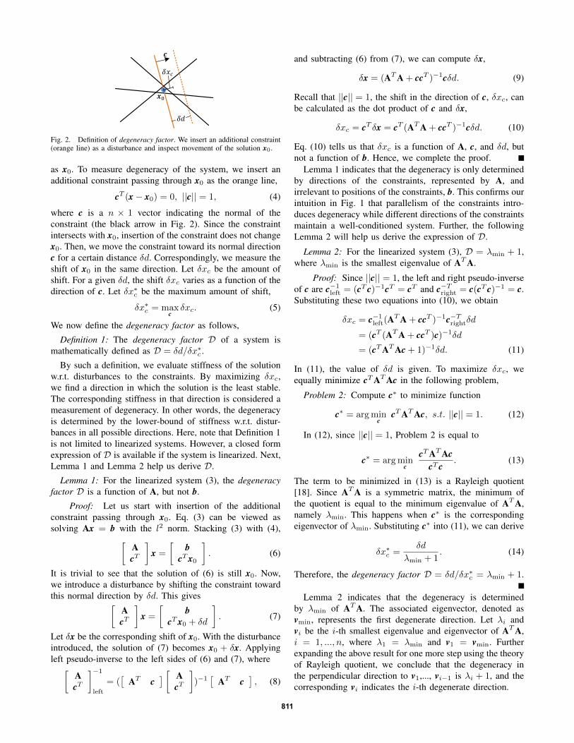
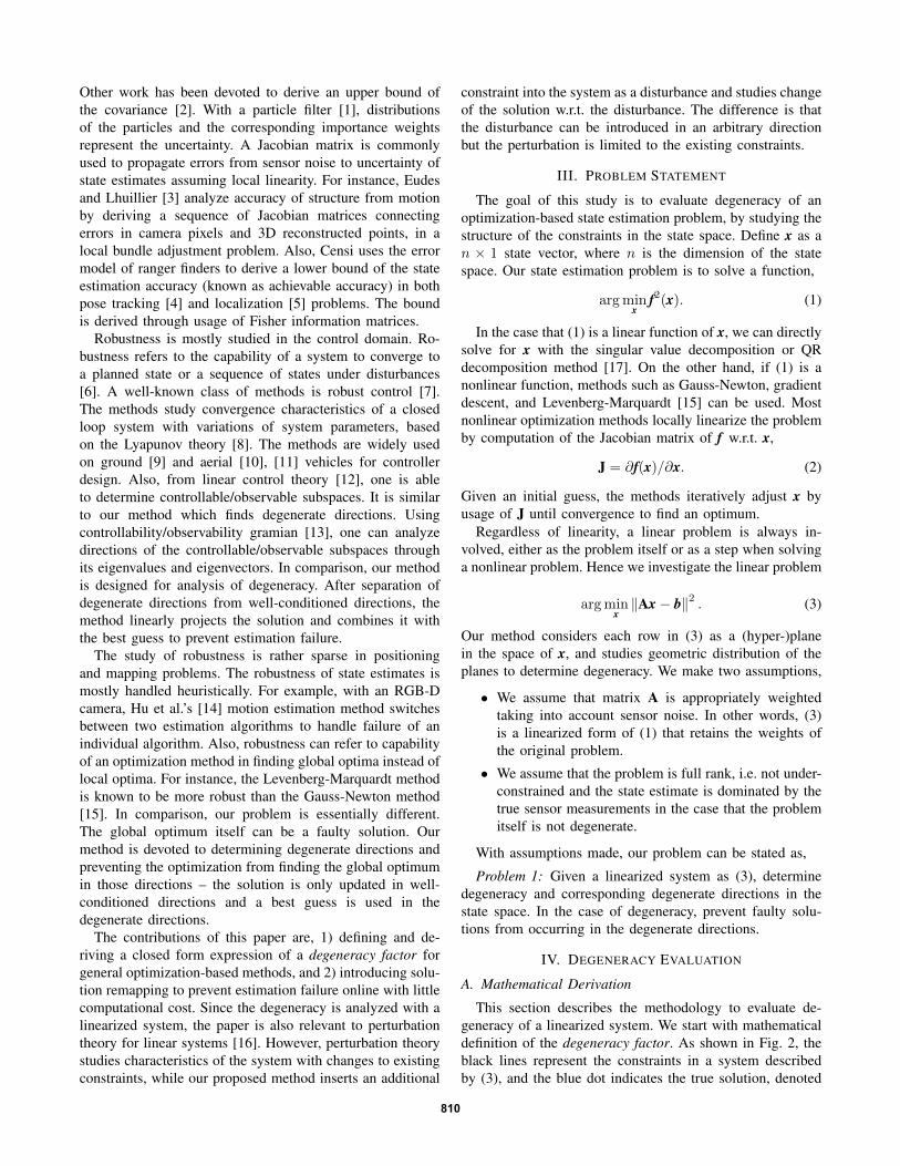
Fig. 2. Definition of degeneracy factor. We insert an additional constraint(orange line) as a disturbance and inspect movement of the solution x0.

as x0. To measure degeneracy of the system, we insert anadditional constraint passing through x0 as the orange line,

cT (x− x0) = 0, ||c|| = 1, (4)

where c is a n × 1 vector indicating the normal of theconstraint (the black arrow in Fig. 2). Since the constraintintersects with x0, insertion of the constraint does not changex0. Then, we move the constraint toward its normal directionc for a certain distance δd. Correspondingly, we measure theshift of x0 in the same direction. Let δxc be the amount ofshift. For a given δd, the shift δxc varies as a function of thedirection of c. Let δx∗c be the maximum amount of shift,

δx∗c = maxcδxc. (5)

We now define the degeneracy factor as follows,

Definition 1: The degeneracy factor D of a system ismathematically defined as D = δd/δx∗c .

By such a definition, we evaluate stiffness of the solutionw.r.t. disturbances to the constraints. By maximizing δxc,we find a direction in which the solution is the least stable.The corresponding stiffness in that direction is considered ameasurement of degeneracy. In other words, the degeneracyis determined by the lower-bound of stiffness w.r.t. distur-bances in all possible directions. Here, note that Definition 1is not limited to linearized systems. However, a closed formexpression of D is available if the system is linearized. Next,Lemma 1 and Lemma 2 help us derive D.

Lemma 1: For the linearized system (3), the degeneracyfactor D is a function of A, but not b.

Proof: Let us start with insertion of the additionalconstraint passing through x0. Eq. (3) can be viewed assolving Ax = b with the l2 norm. Stacking (3) with (4),[

AcT

]x =

[b

cT x0

]. (6)

It is trivial to see that the solution of (6) is still x0. Now,we introduce a disturbance by shifting the constraint towardthis normal direction by δd. This gives[

AcT

]x =

[b

cT x0 + δd

]. (7)

Let δx be the corresponding shift of x0. With the disturbanceintroduced, the solution of (7) becomes x0 + δx. Applyingleft pseudo-inverse to the left sides of (6) and (7), where[

AcT

]−1left

= ([

AT c] [ A

cT

])−1

[AT c

], (8)

and subtracting (6) from (7), we can compute δx,

δx = (AT A + ccT )−1cδd. (9)

Recall that ||c|| = 1, the shift in the direction of c, δxc, canbe calculated as the dot product of c and δx,

δxc = cT δx = cT (AT A + ccT )−1cδd. (10)

Eq. (10) tells us that δxc is a function of A, c, and δd, butnot a function of b. Hence, we complete the proof.

Lemma 1 indicates that the degeneracy is only determinedby directions of the constraints, represented by A, andirrelevant to positions of the constraints, b. This confirms ourintuition in Fig. 1 that parallelism of the constraints intro-duces degeneracy while different directions of the constraintsmaintain a well-conditioned system. Further, the followingLemma 2 will help us derive the expression of D.

Lemma 2: For the linearized system (3), D = λmin + 1,where λmin is the smallest eigenvalue of AT A.

Proof: Since ||c|| = 1, the left and right pseudo-inverseof c are c−1left = (cT c)−1cT = cT and c−Tright = c(cT c)−1 = c.Substituting these two equations into (10), we obtain

δxc = c−1left(AT A + ccT )−1c−Trightδd

= (cT (AT A + ccT )c)−1δd

= (cT AT Ac + 1)−1δd. (11)

In (11), the value of δd is given. To maximize δxc, weequally minimize cT AT Ac in the following problem,

Problem 2: Compute c∗ to minimize function

c∗ = arg minc

cT AT Ac, s.t. ||c|| = 1. (12)

In (12), since ||c|| = 1, Problem 2 is equal to

c∗ = arg minc

cT AT AccT c

. (13)

The term to be minimized in (13) is a Rayleigh quotient[18]. Since AT A is a symmetric matrix, the minimum ofthe quotient is equal to the minimum eigenvalue of AT A,namely λmin. This happens when c∗ is the correspondingeigenvector of λmin. Substituting c∗ into (11), we can derive

δx∗c =δd

λmin + 1. (14)

Therefore, the degeneracy factor D = δd/δx∗c = λmin + 1.

Lemma 2 indicates that the degeneracy is determinedby λmin of AT A. The associated eigenvector, denoted asvmin, represents the first degenerate direction. Let λi andvi be the i-th smallest eigenvalue and eigenvector of AT A,i = 1, ..., n, where λ1 = λmin and v1 = vmin. Furtherexpanding the above result for one more step using the theoryof Rayleigh quotient, we conclude that the degeneracy inthe perpendicular direction to v1,..., vi−1 is λi + 1, and thecorresponding vi indicates the i-th degenerate direction.

811

 

   

 

 

 

 

 

 

  

  

 

Global minima 

True state 

(b) 

(a)                                                          (c) 

(a)

 

   

 

   

 

 

 

 

  

  

 

Global minimum 

True state 

(b)

Fig. 3. (a) Illustration of solution remapping in a linear problem. (b) Anexample of solution remapping applied to a nonlinear problem.

B. Solution Remapping

In this section, we introduce a simple technique which wecall solution remapping to handle degeneracy. We start witha linear problem and then discuss usage of the technique ina nonlinear problem. We first find a number m, 0 ≤ m ≤ n,of eigenvalues λ1,..., λm that are smaller than a threshold.Here, m = 0 indicates a well-conditioned system and m = nindicates a completely degenerate system. Let us constructthree matrices as follows,

Vp = [v1, ..., vm, 0, ..., 0]T , (15)

Vu = [0, ..., 0, vm+1, ..., vn]T , (16)

Vf = [v1, ..., vm, vm+1, ..., vn]T . (17)

Following the convention of Kalman filters, let us definexp as a prediction which is the best guess of the true state. Letxu be an update obtained from solving the system equationdescribed in (3). Here, note that even though the problemis degenerate, (3) is still solvable and yields a solution dueto noise contained in the system. The key idea of solutionremapping is to use xp in the degenerate directions, v1,...,vm, and xu in the well-conditioned directions, vm+1,..., vn.The final solution, xf , is a linear combination of xp and xu,

xf = x′p + x′u, (18)

where x′p = V−1f Vpxp and x′u = V−1f Vuxu.Fig. 3(a) explains the intuition behind solution remapping,

in a two dimensional example. The black axes representthe eigenvectors of a system and the lengths of the axesindicate the eigenvalues. In this example, v1 is a degeneratedirection and v2 is a well-conditioned direction. With (18),we project xp onto v1 to obtain x′p, and xu onto v2 toobtain x′u. Finally, xf is the vector sum of x′p and x′u. Here,

Algorithm 1: Nonlinear Solver with Solution Remapping1 input : f (nonlinear function), xp (predicted solution)2 output : xf (final solution)3 begin4 xf ← xp; O(∗)5 Linearize f at xp to get A, b, and AT A; O(∗)6 Compute λi and vi of AT A, i = 1, ..., n; O(n3)7 Determine a number m of λi smaller than a threshold,

construct Vp, Vu, and Vf based on (15)-(17); O(n2)8 while nonlinear iterations do O(kn2 + ∗)9 Compute update ∆xu; O(∗)

10 xf ← xf + V−1f Vp∆xu; O(n2)

11 end12 Return xf ;13 end

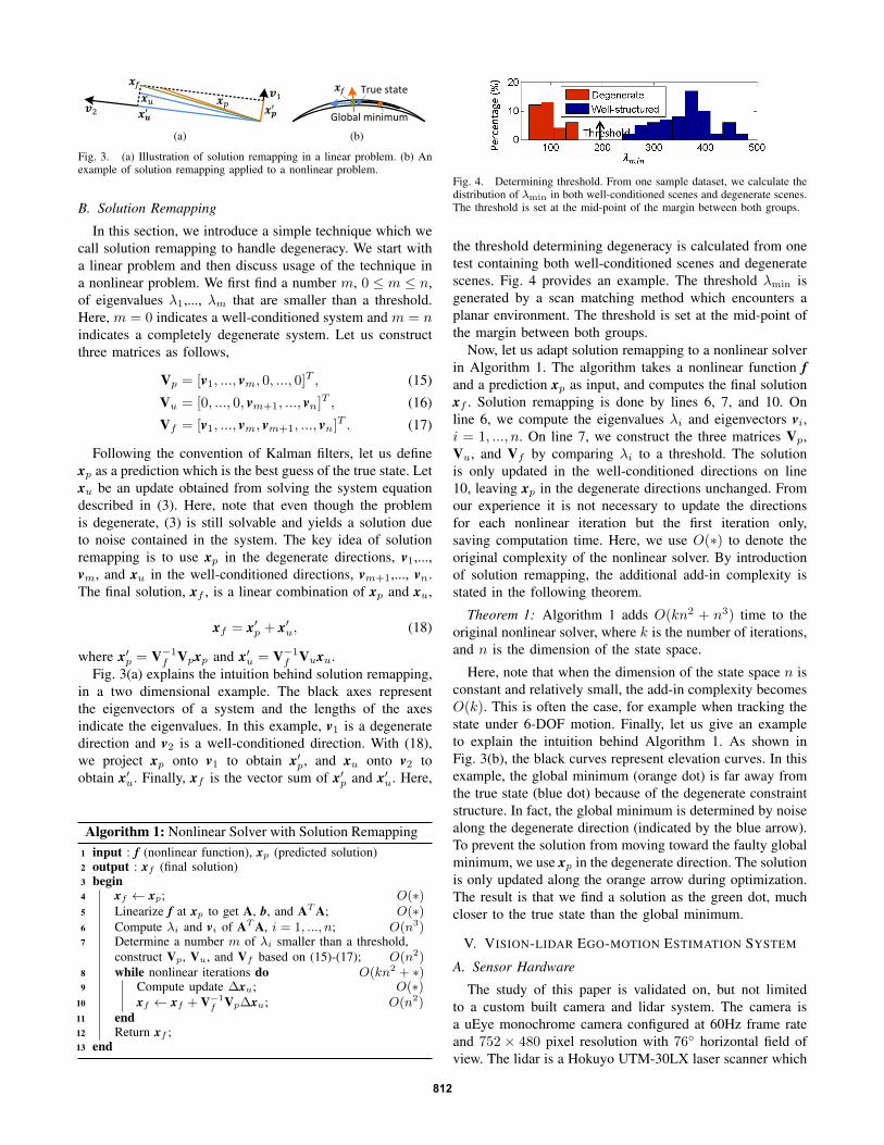
Fig. 4. Determining threshold. From one sample dataset, we calculate thedistribution of λmin in both well-conditioned scenes and degenerate scenes.The threshold is set at the mid-point of the margin between both groups.

the threshold determining degeneracy is calculated from onetest containing both well-conditioned scenes and degeneratescenes. Fig. 4 provides an example. The threshold λmin isgenerated by a scan matching method which encounters aplanar environment. The threshold is set at the mid-point ofthe margin between both groups.

Now, let us adapt solution remapping to a nonlinear solverin Algorithm 1. The algorithm takes a nonlinear function fand a prediction xp as input, and computes the final solutionxf . Solution remapping is done by lines 6, 7, and 10. Online 6, we compute the eigenvalues λi and eigenvectors vi,i = 1, ..., n. On line 7, we construct the three matrices Vp,Vu, and Vf by comparing λi to a threshold. The solutionis only updated in the well-conditioned directions on line10, leaving xp in the degenerate directions unchanged. Fromour experience it is not necessary to update the directionsfor each nonlinear iteration but the first iteration only,saving computation time. Here, we use O(∗) to denote theoriginal complexity of the nonlinear solver. By introductionof solution remapping, the additional add-in complexity isstated in the following theorem.

Theorem 1: Algorithm 1 adds O(kn2 + n3) time to theoriginal nonlinear solver, where k is the number of iterations,and n is the dimension of the state space.

Here, note that when the dimension of the state space n isconstant and relatively small, the add-in complexity becomesO(k). This is often the case, for example when tracking thestate under 6-DOF motion. Finally, let us give an exampleto explain the intuition behind Algorithm 1. As shown inFig. 3(b), the black curves represent elevation curves. In thisexample, the global minimum (orange dot) is far away fromthe true state (blue dot) because of the degenerate constraintstructure. In fact, the global minimum is determined by noisealong the degenerate direction (indicated by the blue arrow).To prevent the solution from moving toward the faulty globalminimum, we use xp in the degenerate direction. The solutionis only updated along the orange arrow during optimization.The result is that we find a solution as the green dot, muchcloser to the true state than the global minimum.

V. VISION-LIDAR EGO-MOTION ESTIMATION SYSTEM

A. Sensor Hardware

The study of this paper is validated on, but not limitedto a custom built camera and lidar system. The camera isa uEye monochrome camera configured at 60Hz frame rateand 752 × 480 pixel resolution with 76◦ horizontal field ofview. The lidar is a Hokuyo UTM-30LX laser scanner which

812

 

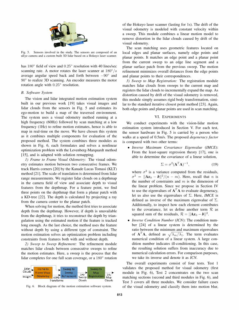
Fig. 5. Sensors involved in the study. The sensors are composed of anuEye camera and a custom built 3D lidar based on a Hokuyo laser scanner.

has 180◦ field of view and 0.25◦ resolution with 40 lines/secscanning rate. A motor rotates the laser scanner at 180◦/saverage angular speed back and forth between −90◦ and90◦ to realize 3D scanning. An encoder measures the motorrotation angle with 0.25◦ resolution.

B. Software System

The vision and lidar integrated motion estimation systembuilt in our previous work [19] takes visual images andlidar clouds from the sensors in Fig. 5 and estimates itsego-motion to build a map of the traversed environment.The system uses a visual odometry method running at ahigh frequency (60Hz) followed by scan matching at a lowfrequency (1Hz) to refine motion estimates, hence is able tomap in real-time on the move. We have chosen this systemas it combines multiple components for evaluation of theproposed method. The system combines three modules asshown in Fig. 6, each formulates and solves a nonlinearoptimization problem with the Levenberg-Marquardt method[15], and is adapted with solution remapping.

1) Frame to Frame Visual Odometry: The visual odom-etry estimates motion between two consecutive frames. Wetrack Harris corners [20] by the Kanade Lucas Tomasi (KLT)method [21]. The scale of translation is determined from lidarrange measurements. We register lidar clouds on a depthmapin the camera field of view and associate depth to visualfeatures from the depthmap. For a feature point, we findthree points on the depthmap that form a planar patch witha KD-tree [22]. The depth is calculated by projecting a rayfrom the camera center to the planar patch.

When solving for motion, the method first tries to associatedepth from the depthmap. However, if depth is unavailablefrom the depthmap, it tries to reconstruct the depth by trian-gulation using the estimated motion if the feature is trackedlong enough. As the last choice, the method uses the featurewithout depth by using a different type of constraint. Themotion estimation solves an optimization problem includingconstraints from features both with and without depth.

2) Sweep to Sweep Refinement: The refinement modulematches lidar clouds between consecutive sweeps to refinethe motion estimates. Here, a sweep is the process that thelidar completes for one full scan coverage, or a 180◦ rotation

 Fig. 6. Block diagram of the motion estimation software system.

of the Hokuyo laser scanner (lasting for 1s). The drift of thevisual odometry is modeled with constant velocity withina sweep. This module combines a linear motion model toremove distortion in the lidar clouds caused by drift of thevisual odometry.

The scan matching uses geometric features located onlocal edges and planar surfaces, namely edge points andplanar points. It matches an edge point and a planar pointfrom the current sweep to an edge line segment and aplanar surface patch from the previous sweep. The motionrefinement minimizes overall distances from the edge pointsand planar points to their correspondences.

3) Sweep to Map Registration: The registration modulematches lidar clouds from sweeps to the current map andregisters the lidar clouds to incrementally expand the map. Asdistortion caused by drift of the visual odometry is removed,this module simply assumes rigid body transformation, simi-lar to the standard iterative closest point method [23]. Again,both edge points and planar points are used in scan matching.

VI. EXPERIMENTS

We conduct experiments with the vision-lidar motionestimation system introduced in Section V. For each test,the sensor hardware in Fig. 5 is carried by a person whowalks at a speed of 0.5m/s. The proposed degeneracy factoris compared with two other terms:• Inverse Maximum Covariance Eigenvalue (IMCE):

From the least-square regression theory [17], one isable to determine the covariance of a linear solution,

Σ = σ2(AT A)−1, (19)

where σ2 is a variance computed from the residuals,σ2 = ||Ax0 − b||2/(n − m). Here, recall that n isthe number of constraints and m is the dimension ofthe linear problem. Since we propose in Section IVto use the eigenvalues of AT A to evaluate degeneracy,let us also use the eigenvalues of Σ. Here, IMCE isdefined as inverse of the maximum eigenvalue of Σ.Additionally, to inspect how each element contributesto the covariance, let us define another term R assquared sum of the residuals, R = ||Ax0 − b||2.

• Inverse Condition Number (ICN): The condition num-ber [24] of a linear system is determined by theratio between the minimum and maximum eigenvaluesof AT A, defined as

√λm/λ1. The term evaluates

numerical condition of a linear system. A large con-dition number indicates ill-conditioning. In this case,the resulting solution suffers from inaccuracy due tonumerical calculation errors. For comparison purposes,we take its inverse and denote it as ICN.

The overall experiments consist of four tests. Test 1validates the proposed method for visual odometry (firstmodule in Fig. 6), Test 2 concentrates on the two scanmatching sections (second and third modules in Fig. 6), andTest 3 covers all three modules. We consider failure casesof the visual odometry and classify them into motion blur,

813

dynamic environment, and feature-poor scene. We think thatmotion blur can be handled by a fast camera and image framerate, and dynamic environments can be addressed by outlierrejection or distraction suppression technique [25]. A feature-poor scene is the most relevant to degeneracy. Typically, thisoccurs where the camera faces a texture-less environment,points to the sun, or is in a dark environment. Likely, fewfeatures are available or the features are extracted from aconcentrated area within the images.

With such consideration, Test 1 is conducted in a corridor.As shown in Fig. 7, the path goes through two feature-poorcorners labeled with numbers 1 and 2. Fig. 7(a) presentsthe estimated trajectory and the map built when degeneracyis eliminated by solution remapping (Algorithm 1). Here,prediction is provided by a constant velocity model. Fig. 7(b)shows one sample image from each of the labeled cor-ners. In Fig. 7(c)-(d), we show the eigenvectors of matrixAT A corresponding to the two images in Fig. 7(c). Darkerblocks indicate larger values, and rows in top-down ordercorrespond to small to large eigenvalues. The directionsabove the red lines are degenerate. Careful comparison findsthat in location 1, the most degenerate direction is lateraltranslation (the darkest block on the first row is labeled with“L: left”). This makes sense as features in location 1 arevertically distributed, resulting in lateral translation to bepoorly constrained. Correspondingly, the red trajectory jumpsleftward. In location 2, Fig. 7(d) indicates degeneracy mostlyin vertical translation (the darkest block on the first row islabeled with “U: up”). This is because the features spanhorizontally. Accordingly, the red trajectory jumps upward.

Next we examine IMCE. In Fig. 7(f), we show the valuesfor both the first and last iterations in the nonlinear optimiza-tion. We see that the values of IMCE are noisy mostly dueto the noisy nature of the squared sum of the residuals R(Fig. 7(g)). Note that the value at the first iteration is moremeaningful as ideally we want to detect degeneracy fromthe beginning of the optimization so that solution remappingcan be introduced. However, we also see IMCE at the firstiteration is much noisier than at the last iteration as R isnot yet minimized. In Fig. 7(h), we show the number ofconstraints, which is also involved in the computation of thecovariance Σ and possibly brings in uncertainty.

Finally we compare ICN and degeneracy factor D inFig. 7(i). Here, ICN is manually scaled to match with D.Further, we compare the ratio of the two terms D/ICN inFig. 7(j). It is apparent that the value of the ratio reducesin locations 1 and 2, indicating D is more effective. Thereason is that ICN calculates the ratio between the minimumand maximum eigenvalues of AT A such that the maximumeigenvalue also has effect on the term. In Fig. 7(k), we showthe maximum eigenvalue λ6 which decreases in locations1 and 2. The reduction of λ6 contributes to the increaseof ICN. Here, the consideration is that degeneracy shouldnot be determined by the well-conditioned directions but bythe degenerate directions themselves. Finally, we show thenumber of degenerate DOF during Test 1 in Fig. 7(l).

Then, in Test 2, we choose an environment which contains

a piece of flat ground as in Fig. 8. Traveling on the flatground results in sliding of the scan matching on the red

(a) Map (b) Image features

(c) Location 1 (d) Location 2 (e)

(f) IMCE at the first and last iterations

(g) R at the first and last iterations

(h) Number of constraints

(i) ICN, D

(j) ICN, D

(k) Maximum eigenvalue of AT A

(l) Number of degenerate DOF

Fig. 7. Test 1: Visual odometry degeneracy in feature-poor environment.

814

curve in Fig. 8(a). Correspondingly, the top three rows ofFig. 8(c)-(d) indicate that degeneracy occurs in the directionsof forward translation, lateral translation, and yaw rotation,meaning that translation parallel to the ground and rotationperpendicular to the ground are poorly constrained.

Looking into the rest of the figure, we find that the valueof IMCE is either noisy or does not decrease obviously(for the sweep to sweep refinement section in Fig. 8(f)and the sweep to map registration section in Fig. 8(g)).Again, this is because IMCE is determined by multiple termsincluding squared sum of the residuals R and the numberof constraints. Here, note that the values of IMCE do notdiffer much between the first and last iterations because thescan matching only refines motion estimates generated bythe visual odometry. The value of R reduces little during thecourse of optimization. Fig. 8(h)-(i) compare ICN and D.We can see an obvious drop of value between 35-70s whenthe degeneracy occurs. In Fig. 8(j), the ratio D/ICN alsodecreases slightly during this interval. In Fig. 8(k), we seethat the method detects three degenerate DOF correspondingto the top three rows in Fig. 8(c)-(d).

Finally, we conduct a larger scale test in Test 3 containingindoor and outdoor environments, as shown in Fig. 9. Thepath starts in front of a building, passes through the buildingand exits to the outside, climbs stairs, and follows a smalltrail to come back and finish at the exact starting position.The overall traveling distance is 538m. The path contains twodegenerate scenes for the visual odometry in locations 1 and3 due to undesirable lighting conditions, and two degeneratescenes for the scan matching in locations 2 and 4. In location2, the lidar sees the flat ground and one wall on its right sidecausing degeneracy in forward translation. In location 4, thelidar only sees the flat ground similar to Test 2. We observethat the value of D drops in locations 1 and 3 in Fig. 9(c)and in locations 2 and 4 in Fig. 9(d)-(e).

Fig. 10 further compares the estimated trajectories. Thegreen curve is without solution remapping, hence jumps oc-cur along the path. The red curve is estimated with consistentmotion prior added to the motion estimation problems. Thevisual odometry section takes motion prior from a constantvelocity model, and each scan matching section takes outputfrom the previous section. Here, the motion prior is givenas little as possible to eliminate degeneracy. However, it stillcauses drift at the end to be about three times as large ason the blue curve (proposed method). Thanks to solutionremapping, the system is able to conquer all degeneracyresulting in a 0.71% relative position error at the end ofthe blue curve compared to the distance traveled.

VII. DISCUSSION

As the solution remapping linearly combines the predic-tion and update, one can argue that this is a variant of theKalman filter. Our response is that a filter handles accuracy,while the proposed method is devoted to degeneracy androbustness. The difference is that filters average multiplenoisy measurements to gain better accuracy. When workingwith degeneracy, we consider the solution to be completely

unusable in the degenerate directions and simply take theprediction instead. Our second response is that solution

(a) Map (b) Lidar scan

(c) Sweep to sweep (d) Sweep to map (e)

(f) IMCE of sweep to sweep refinement section

(g) IMCE of sweep to map registration section

(h) ICN, D of sweep to sweep refinement section

(i) ICN, D of sweep to map registration section

(j) D/ICN for both sections

(k) Number of degenerate DOF

Fig. 8. Test 2: Scan matching degeneracy on flat ground.

815

(a) Map (b) Image features and lidar scans

(c) D of frame to frame visual odometry section (d) D of sweep to sweep refinement section (e) D of sweep to map registration section

Fig. 9. Test 3: Complete test including indoor and outdoor environments. The overall path is 538m long, starting in front of a building, passing throughthe building with stairs and following a trail on hilly terrain to return to the start. The path encounters four degenerate scenes labeled with 1-4.

𝑋  (m)  

𝑌  (m)  𝑍  (m)  

   

6030

0

1007550250-25-50

1510

50

W/O RemappingConst Motion PriorW/ Remapping

End  Start  

1  

2  

3  4  

Fig. 10. Trajectories of Test 3. The green curve is estimated withoutsolution remapping, and jumps occur along the path. The red curve usesconsistent motion prior to eliminate degeneracy. This results in more driftconsequently. The blue curve uses the proposed solution remapping. Theposition error at the end is 0.71% of the 538m trajectory length.

remapping can be adapted to individual iterations of non-linear optimization. A filter only takes the final solutions toseed steps. Finally, a filter can be the following step of theproposed method taking its output for further integration.

VIII. CONCLUSION

Robustness of estimation is critical for state estimationand especially for autonomous vehicles. This paper improvesrobustness by handling environmental degeneracy. A degen-eracy factor is mathematically defined and derived. Degen-eracy is evaluated through computation of the associatedeigenvalues and eigenvectors. When degeneracy occurs, theproposed method automatically separates the state spaceand partially solves the problem only in well-conditioneddirections. In degenerate directions, a best guess is usedinstead. The method is tested with a custom-built visionand lidar system in a number of challenging scenarios, foronline positioning and mapping. Experimental results showthat the system is able to conquer environmentally degeneratemoments, to reliably estimate state, and to use the state tobuild accurate 3D representations of the environment.

REFERENCES

[1] S. Thrun, W. Burgard, and D. Fox, Probabilistic Robotics. Cambridge,MA, The MIT Press, 2005.

[2] Z. Dong and Z. You, “Finite-horizon robust Kalman filtering foruncertain discrete time-varying systems with uncertain-covariancewhite noises,” IEEE Signal Processing Letters, vol. 13, no. 8, pp.493–496, 2006.

[3] A. Eudes and M. Lhuillier, “Error propagations for local bundleadjustment,” in IEEE Conference on Computer Vision and PatternRecognition (CVPR), 2009, pp. 2411–2418.

[4] A. Censi, “On achievable accuracy for pose tracking,” in IEEE Intl.Conf. on Robotics and Automation, 2009, pp. 1–7.

[5] ——, “On achievable accuracy for range-finder localization,” in IEEEIntl. Conf. on Robotics and Automation, 2007, pp. 4170–4175.

[6] A. Isidori, Nonlinear control systems. Springer, 1999, vol. 2.[7] P. Ioannou and J. Sun, Robust adaptive control. Dover Pub., 2012.[8] P. Parks, “A. M. Lyapunov’s stability theory–100 years on,” IMA

Journal of Math. Control and Info., vol. 9, no. 4, pp. 275–303, 1992.[9] Y. Kanayama, Y. Kimura, F. Miyazaki, and T. Noguchi, “A stable

tracking control method for an autonomous mobile robot,” in IEEEIntl. Conf. on Robotics and Automation (ICRA), 1990, pp. 384–389.

[10] J. Fink, N. Michael, S. Kim, and V. Kumar, “Planning and control forcooperative manipulation and transportation with aerial robots,” TheIntl. Journal of Robotics Research, vol. 30, no. 3, pp. 324–334, 2011.

[11] P. Sujit, S. Saripalli, and J. Sousa, “Unmanned aerial vehicle pathfollowing: A survey and analysis of algorithms for fixed-wing un-manned aerial vehicless,” IEEE Control Systems, vol. 34, no. 1, pp.42–59, 2014.

[12] J. J. d’Azzo and C. D. Houpis, Linear control system analysis anddesign: conventional and modern. McGraw-Hill Higher Edu., 1995.

[13] B. Hinson and K. Morgansen, “Observability optimization for thenonholonomic integrator,” in American Control Conference (ACC),June 2013.

[14] G. Hu, S. Huang, L. Zhao, A. Alempijevic, and G. Dissanayake, “Arobust RGB-D SLAM algorithm,” in IEEE/RSJ Intl. Conf. on Intel.Robots and Systems (IROS), Vilamoura, Portugal, Oct. 2012.

[15] J. Nocedal and S. Wright, Numerical Optimization. New York,Springer-Verlag, 2006.

[16] S. Chandrasekaran and I. Ipsen, “Perturbation theory for the solutionof systems of linear equations,” Yale University, Tech. Rep., 1991.

[17] L. Trefethen and D. B. III, Numerical linear algebra. SIAM, 1997.[18] R. A. Horn and C. R. Johnson, Matrix analysis. Cambridge university

press, 2012.[19] J. Zhang and S. Singh, “Visual-lidar odometry and mapping: Low-

drift, robust, and fast,” in IEEE International Conference on Roboticsand Automation (ICRA), May 2015.

[20] R. Hartley and A. Zisserman, Multiple View Geometry in ComputerVision. New York, Cambridge University Press, 2004.

[21] B. Lucas and T. Kanade, “An iterative image registration techniquewith an application to stereo vision,” in Proceedings of ImagingUnderstanding Workshop, 1981, pp. 121–130.

[22] M. de Berg, M. van Kreveld, M. Overmars, and O. Schwarzkopf,Computation Geometry: Algorithms and Applications. Springer, 2008.

[23] F. Pomerleau, F. Colas, R. Siegwart, and S. Magnenat, “ComparingICP variants on real-world data sets,” Autonomous Robots, 2013.

[24] E. Cheney and D. Kincaid, Numerical mathematics and computing.Cengage Learning (6th Edition), 2007.

[25] C. McManus, W. Churchill, A. Napier, B. Davis, and P. Newman,“Distraction suppression for vision-based pose estimation at cityscales,” in Robotics and Automation (ICRA), 2013 IEEE InternationalConference on, 2013, pp. 3762–3769.

816