Optimization Of Zonal Wavefront Estimation And Curvature ...

University of Central Florida University of Central Florida

STARS STARS

Electronic Theses and Dissertations, 2004-2019

2007

Optimization Of Zonal Wavefront Estimation And Curvature Optimization Of Zonal Wavefront Estimation And Curvature

Measurements Measurements

Weiyao Zou University of Central Florida

Part of the Electromagnetics and Photonics Commons, and the Optics Commons

Find similar works at: https://stars.library.ucf.edu/etd

University of Central Florida Libraries http://library.ucf.edu

This Doctoral Dissertation (Open Access) is brought to you for free and open access by STARS. It has been accepted

for inclusion in Electronic Theses and Dissertations, 2004-2019 by an authorized administrator of STARS. For more

information, please contact [email protected].

STARS Citation STARS Citation Zou, Weiyao, "Optimization Of Zonal Wavefront Estimation And Curvature Measurements" (2007). Electronic Theses and Dissertations, 2004-2019. 3432. https://stars.library.ucf.edu/etd/3432

https://stars.library.ucf.edu/



https://stars.library.ucf.edu/etd

http://network.bepress.com/hgg/discipline/271?utm_source=stars.library.ucf.edu%2Fetd%2F3432&utm_medium=PDF&utm_campaign=PDFCoverPages

http://network.bepress.com/hgg/discipline/204?utm_source=stars.library.ucf.edu%2Fetd%2F3432&utm_medium=PDF&utm_campaign=PDFCoverPages

https://stars.library.ucf.edu/etd

http://library.ucf.edu/

mailto:[email protected]

https://stars.library.ucf.edu/etd/3432?utm_source=stars.library.ucf.edu%2Fetd%2F3432&utm_medium=PDF&utm_campaign=PDFCoverPages



OPTIMIZATION OF ZONAL WAVEFRONT ESTIMATION AND

CURVATURE MEASUREMENTS

by

WEIYAO ZOU B.S. Tianjin University, China

M.S. Chinese Academy of Sciences, China

A dissertation submitted in partial fulfillment of the requirements for the degree of Doctor of Philosophy in the College of Optics and Photonics

at the University of Central Florida Orlando, Florida

Spring Term 2007

Major Professor: Jannick P. Rolland

ii

© 2007 Weiyao Zou

ABSTRACT

Optical testing in adverse environments, ophthalmology and applications where

characterization by curvature is leveraged all have a common goal: accurately estimate

wavefront shape. This dissertation investigates wavefront sensing techniques as applied to

optical testing based on gradient and curvature measurements. Wavefront sensing involves the

ability to accurately estimate shape over any aperture geometry, which requires establishing a

sampling grid and estimation scheme, quantifying estimation errors caused by measurement

noise propagation, and designing an instrument with sufficient accuracy and sensitivity for the

application.

Starting with gradient-based wavefront sensing, a zonal least-squares wavefront

estimation algorithm for any irregular pupil shape and size is presented, for which the normal

matrix equation sets share a pre-defined matrix. A Gerchberg–Saxton iterative method is

employed to reduce the deviation errors in the estimated wavefront caused by the pre-defined

matrix across discontinuous boundary. The results show that the RMS deviation error of the

estimated wavefront from the original wavefront can be less than λ/130~ λ/150 (for λ equals

632.8nm) after about twelve iterations and less than λ/100 after as few as four iterations. The

presented approach to handling irregular pupil shapes applies equally well to wavefront

estimation from curvature data.

A defining characteristic for a wavefront estimation algorithm is its error propagation

behavior. The error propagation coefficient can be formulated as a function of the eigenvalues of

the wavefront estimation-related matrices, and such functions are established for each of the

basic estimation geometries (i.e. Fried, Hudgin and Southwell) with a serial numbering scheme,

ii

where a square sampling grid array is sequentially indexed row by row. The results show that

with the wavefront piston-value fixed, the odd-number grid sizes yield lower error propagation

than the even-number grid sizes for all geometries. The Fried geometry either allows sub-sized

wavefront estimations within the testing domain or yields a two-rank deficient estimation matrix

over the full aperture; but the latter usually suffers from high error propagation and the waffle

mode problem. Hudgin geometry offers an error propagator between those of the Southwell and

the Fried geometries. For both wavefront gradient-based and wavefront difference-based

estimations, the Southwell geometry is shown to offer the lowest error propagation with the

minimum-norm least-squares solution. Noll’s theoretical result, which was extensively used as a

reference in the previous literature for error propagation estimate, corresponds to the Southwell

geometry with an odd-number grid size.

For curvature-based wavefront sensing, a concept for a differential Shack-Hartmann (DSH)

curvature sensor is proposed. This curvature sensor is derived from the basic Shack-Hartmann

sensor with the collimated beam split into three output channels, along each of which a lenslet

array is located. Three Hartmann grid arrays are generated by three lenslet arrays. Two of the

lenslets shear in two perpendicular directions relative to the third one. By quantitatively

comparing the Shack-Hartmann grid coordinates of the three channels, the differentials of the

wavefront slope at each Shack-Hartmann grid point can be obtained, so the Laplacian curvatures

and twist terms will be available. The acquisition of the twist terms using a Hartmann-based

sensor allows us to uniquely determine the principal curvatures and directions more accurately

than prior methods. Measurement of local curvatures as opposed to slopes is unique because

curvature is intrinsic to the wavefront under test, and it is an absolute as opposed to a relative

measurement. A zonal least-squares-based wavefront estimation algorithm was developed to

iii

estimate the wavefront shape from the Laplacian curvature data, and validated. An

implementation of the DSH curvature sensor is proposed and an experimental system for this

implementation was initiated.

The DSH curvature sensor shares the important features of both the Shack-Hartmann slope

sensor and Roddier’s curvature sensor. It is a two-dimensional parallel curvature sensor. Because

it is a curvature sensor, it provides absolute measurements which are thus insensitive to

vibrations, tip/tilts, and whole body movements. Because it is a two-dimensional sensor, it does

not suffer from other sources of errors, such as scanning noise. Combined with sufficient

sampling and a zonal wavefront estimation algorithm, both low and mid frequencies of the

wavefront may be recovered. Notice that the DSH curvature sensor operates at the pupil of the

system under test, therefore the difficulty associated with operation close to the caustic zone is

avoided. Finally, the DSH-curvature-sensor-based wavefront estimation does not suffer from the

2π-ambiguity problem, so potentially both small and large aberrations may be measured.

iv

To my parents, who have been patiently supporting me for my studying since my young age!

To my grandparents, who love me so much as always!

To my sisters, who love me and encourage me all the time!

ACKNOWLEDGMENTS

I cordially thank my advisor, Dr. Jannick Rolland, for her support and guidance on my

graduate study towards a PhD in CREOL and motivating me to conduct this research. I want to

give my heartfelt thanks to Dr. Kevin Thompson at Optical Research Associates for his

stimulating discussions on optical testing and his insightful comments and guidance for my

dissertation. I also want to greatly thank my dissertation committee members, Dr. Glenn

Boreman, Dr. Emil Wolf, Dr. James Harvey and Dr. Larry Andrews for their dedication and

comments provided for this work. I would like to thank Dr. Eric Clarkson at the University of

Arizona for his comments regarding one of the statistical methods used in this research. I would

like to thank Paul Glenn for sharing his experience on the development of his own profiling

curvature sensor.

I would like to thank Dr. Yonggang Ha of the ODALab for his help on ray tracing in the

experimental system design for curvature measurements and Mr. Ozan Cakmakci for offering

generously his time to discuss some algorithms with me. I would like to thank the other ODALab

members, Dr. Avni Ceyhun Akcay, Dr. Vesselin Shaoulov, Mr. Kye-Sung Lee, Dr. Anand

Santhanam, Dr. Cali Fidopiastis, Ms. Supraja Murali, Mr. Ricardo Martins, Mr. Florian Fournier,

Mr. Panomsak Meemon, Mr. Costin Curatu, Mr. Mohamed Salem and Ms. Nicolene Papp for

their friendships. I would like to also thank all my friends in CREOL and in the United States,

who shared their friendships generously.

My very special thanks go to my dear family: my father, my mother, my three sisters, my

grandparents, my uncles and aunts, and all my other relatives for their love, patience, persistent

ii

support and sacrifice, and long-time pains suffered for my studying and career pursuit in China

and in the United States.

The work presented in this dissertation was funded in part by the National Science

Foundation grant IIS/HCI-0307189.

TABLE OF CONTENTS

LIST OF FIGURES ......................................................................................................................... i

LIST OF TABLES........................................................................................................................... i

LIST OF ACRONYMS/ABBREVIATIONS.................................................................................. i

CHAPTER ONE: INTRODUCTION............................................................................................. 3

1.1 Historical review of optical testing ....................................................................................... 3

1.1.1 Hartmann test ................................................................................................................. 4

1.1.2 Shack-Hartmann sensor and Pyramid wavefront sensor ............................................... 6

1.1.3 Interferometric tests ..................................................................................................... 10

1.2 Recovery of the mid-spatial frequency: Modal or Zonal? .................................................. 12

1.3 Vibrational effects............................................................................................................... 15

1.4 Motivation........................................................................................................................... 16

1.5 Dissertation outline ............................................................................................................. 17

CHAPTER TWO: REVIEW OF CURVARTURE SENSING .................................................... 20

2.1 Roddier’s wavefront curvature sensor ................................................................................ 20

2.1.1 Methodology evolution................................................................................................ 22

2.1.2 Implementations........................................................................................................... 25

2.1.3 Advantages and disadvantages .................................................................................... 26

2.2 Special wavefront curvature sensors................................................................................... 27

2.2.1 CGS wavefront curvature sensor ................................................................................. 28

2.2.2 Hybrid wavefront curvature sensor.............................................................................. 31

2.2.3 Curvature profiling technique ...................................................................................... 32

ii

2.3 Summary ............................................................................................................................. 35

CHAPTER THREE: REVIEW OF WAVEFRONT ESTIMATION TECHNIQUES................. 36

3.1 Neumann boundary problem in wavefront estimation........................................................ 36

3.2 Slope-based wavefront estimations..................................................................................... 39

3.2.1 Zonal slope-based wavefront estimation ..................................................................... 40

3.2.1.1 Least-squares fitting method................................................................................. 42

3.2.1.2 Fourier transform method ..................................................................................... 44

3.2.2 Modal slope-based wavefront estimation .................................................................... 46

3.2.2.3 Least-squares based modal estimation.................................................................. 48

3.2.2.4 Fourier transform-based modal estimation ........................................................... 51

3.2.3 Radon transform-based modal estimation ................................................................... 53

3.3 Curvature-based wavefront estimations.............................................................................. 54

3.3.1 Zonal curvature-based wavefront estimation............................................................... 55

3.3.1.1 Least-squares-based zonal estimation................................................................... 56

3.3.1.2 Fourier transform-based zonal estimation ............................................................ 56

3.3.2 Modal curvature-based wavefront estimation.............................................................. 58

3.4 Phase retrieval techniques................................................................................................... 61

3.4.1 Gerchberg-Saxton and Misell methods........................................................................ 63

3.4.1.1 Gerchberg-Saxton method .................................................................................... 63

3.4.1.2 Misell algorithm.................................................................................................... 65

3.4.2 Phase diversity technique............................................................................................. 67

3.5 Comparisons and Summary ................................................................................................ 69

3.5.1 Phase diversity technique and the S-H sensor ............................................................. 69

iii

3.5.2 Phase diversity technique and Roddier’s curvature sensor.......................................... 70

3.5.3 Summary ...................................................................................................................... 71

CHAPTER FOUR: ITERATIVE SLOPE-BASED WAVEFRONT ESTIMATION FOR ANY

SHAPED PUPILS......................................................................................................................... 72

4.1 Proposed wavefront estimation algorithm for any size and pupil shape ...................... 73

4.1.1 Pre-defined matrix equation for wavefront estimation ................................................ 73

4.1.2 Wavefront slope computations .................................................................................... 78

4.1.2.1 Wavefront y-slope computation............................................................................ 78

4.1.2.2 Wavefront z-slope computation............................................................................ 80

4.1.3 Least-squares -based Gerchberg-Saxton iterative algorithm ....................................... 82

4.2 Examples and Results ................................................................................................... 85

4.2.1 Case 1: Circular pupil without central obscuration...................................................... 86

4.2.2 Case 2: Circular pupil with a 10% central obscuration................................................ 87

4.2.3 Algorithm convergence................................................................................................ 89

4.3 Computational complexity............................................................................................ 90

4.3.1 Computational complexity of the proposed iterative algorithm .................................. 90

4.3.1.1 Spatial complexity ................................................................................................ 91

4.3.1.2 Time complexity (Impact on computation time) .................................................. 91

4.3.2 Complexity comparison with the FFT-based iterative algorithms .............................. 93

4.3.2.1 Comparison of time complexity............................................................................ 93

4.3.2.2 Comparison of spatial complexity ........................................................................ 94

4.4 Error propagation estimation ........................................................................................ 95

4.5 Summary ....................................................................................................................... 99

iv

CHAPTER FIVE: QUANTIFICATIONS OF ERROR PROPAGATION IN WAVEFRONT

ESTIMATION ............................................................................................................................ 101

5.1 Introduction................................................................................................................. 101

5.2 Brief review of previous work .................................................................................... 103

5.3 Formulation of the error propagation with matrix method ......................................... 105

5.4 Quantification of Wavefront difference-based error propagation .............................. 108

5.4.1 Wavefront difference-based error propagators ................................................... 109

5.4.1.1 Hudgin Geometry............................................................................................ 109

5.4.1.2 Southwell Geometry ....................................................................................... 113

5.4.1.3 Fried Geometry ............................................................................................... 116

5.4.2 Comparisons of the error propagators................................................................. 119

5.5 Quantification of wavefront slope-based error propagation ....................................... 122

5.6 Summary ..................................................................................................................... 125

CHAPTER SIX: DIFERRENTIAL SHACK-HARTMANN CURVATURE SENSOR ........... 126

6.1 Slope differential measurements................................................................................. 127

6.2 Implementation of the DSH curvature sensor............................................................. 130

6.3 Experimental setup for the DSH curvature sensor...................................................... 132

6.4 Curvature-based zonal wavefront estimation.............................................................. 137

6.5 Principal curvature computations ............................................................................... 142

6.6 Summary ..................................................................................................................... 145

CHAPTER SEVEN: SIMULATION AND ERROR ANALYSIS............................................. 147

7.1 Numerical validation of the proposed algorithm .............................................................. 147

7.2 Error analysis of wavefront measurement ........................................................................ 153

v

7.2.1 Dynamic range ........................................................................................................... 154

7.2.2 Sensitivity .................................................................................................................. 155

7.2.3 Accuracy .................................................................................................................... 156

7.3 Summary ........................................................................................................................... 158

CHAPTER EIGHT: SUMMARY OF CONTRIBUTIONS AND CONCLUSION................... 159

APPENDIX DERIVATION OF EQS. (4.11), (4. 12), (4.26) AND (4. 27) .............................. 163

LIST OF REFERENCES............................................................................................................ 167

LIST OF FIGURES

Figure 1.1 Hartmann test (Adopted from D. Malacara)................................................................. 5

Figure 1.2 (a) The concept of the S-H sensor and (b) a sampling grid.......................................... 7

Figure 1.3 The spot centroiding in a quad cell in a CCD target .................................................... 8

Figure 1.4 Quad cell in S-H WFS versus quadrant in pyramid WFS (Adopted from Bauman) .. 9

Figure 2.1 The illustration of Roddier’s curvature sensing (from Malacara) ............................... 21

Figure 2.2 Schematic for a reflection CGS curvature sensor (Adopted from Kolawa)............... 29

Figure 2.3 The principle of a CSG curvature sensor (from Kolawa, et al).................................. 30

Figure 2.4 The foci in the hybrid wavefront curvature sensor..................................................... 32

Figure 2.5 The differential measurement of slope (Adopted from Glenn) ................................. 33

Figure 2.6 Schematic layout of the curvature profiling instrument (Adopted from Glenn) ....... 34

Figure 3.1 The testing aperture for wavefront estimation............................................................. 37

Figure 3.2 Sampling geometries for wavefront estimation......................................................... 39

Figure 3.3 Five-point stencil ....................................................................................................... 40

Figure 3.4 The flow chart of Gerchberg’s fringe extrapolation algorithm. (from Roddier &

Roddier 1987) ....................................................................................................................... 45

Figure 3.5 An example of interferogram extrapolation (from Roddier & Roddier1987) (a)

Interferogram before fringe extrapolation (b) Interferogram after fringe extrapolation....... 45

Figure 3.6 Flow Chart for the iterative FT-based wavefront estimation from slope data (from

Roddier & Roddier 1991) ..................................................................................................... 46

Figure 3.7 Flow Chart of iterative FT-based wavefront estimation from curvature data (from

Roddier & Roddier) .............................................................................................................. 57

ii

Figure 3.8 Gerchberg-Saxton algorithm (Adopted from Chanan)............................................... 64

Figure 3.9 Misell algorithm ......................................................................................................... 66

Figure 3.10 Optical layout of a phase diversity system (from. Paxman et al)............................. 67

Figure 4.1 The double sampling grid systems illustrated in the y-direction................................ 74

Figure 4.2 The domain extension for an irregular-shaped pupil.................................................. 75

Figure 4.3 Non-iterative wavefront estimation with pre-defined matrix..................................... 77

Figure 4.4 Flow chart of the least-squares-based Gerchberg-Saxton-type iterative wavefront

estimation algorithm ............................................................................................................. 84

Figure 4.5 (a) A 30-mm diameter circular pupil within the extended domain 1Ω . (b) The ground-

truth wavefront within the circular pupil 0Ω on a vertical scale of ±1µm........................... 86

Figure 4.6 Wavefront deviation error (on scale of ±1µm) for a 30 mm-diameter circular pupil

with iterations i=0, 1, 2, 3, 4, and 13, respectively (λ=632.8nm). ........................................ 87

Figure 4.7 (a). A 30-mm diameter circular pupil with a 10% central obscuration. (b). A ground-

truth wavefront at this pupil 0Ω on a vertical scale of ±1µm (right). .................................. 88


with a 10% central obscuration through iterations i=0, 1, 2, 3, 4, 10, respectively

(λ=632.8nm).......................................................................................................................... 88

Figure 4.9 Plot of RMS deviation errors as a function of the number of iterations..................... 89

Figure 4.10 The condition number of normal estimation matrix versus grid dimension size. ..... 98

Figure 5.1 Previous results on error propagation........................................................................ 104

Figure 5.2 Grid array with serial numbering scheme ................................................................. 108

Figure 5.3 WFD-based error propagators for the Hudgin geometry .......................................... 112

iii

Figure 5.4 WFD-based error propagators for the Southwell geometry ...................................... 115

Figure 5.5 WFD-based error propagators for the Fried geometry .............................................. 118

Figure 5.6 Comparison of the WDF-based error propagators .................................................... 120

Figure 5.7 Comparison of the slope-based error propagators..................................................... 124

Figure 6.1: The x- and y-differential shears of the Hartmann grid............................................ 129

Figure 6.2: An implementation of the DSH curvature sensor without calibration path ............. 131

Figure 6.3 Optical layout of the experimental system for the DSH curvature sensor ................ 134

Figure 6.4 Picture of the experimental system for the DSH curvature sensor............................ 135

Figure 6.5 GUI of the DSH sensor experimental setup .............................................................. 136

Figure 6.6 A 52-point S-H Grid.................................................................................................. 138

Figure 6.7 The edge points.......................................................................................................... 139

Figure 6.8 The corner points....................................................................................................... 140

Figure 7.1 Wavefront estimation with an 8×8 grid array............................................................ 149

Figure 7. 2 Wavefront estimation with 30×30 grid array ........................................................... 151

Figure 7. 3 Wavefront deviation errors and the defocus values ................................................. 152

Figure 7. 4 Wavefront discretization error versus discretization grid size ................................. 153

LIST OF TABLES

Table 3.1 The Zernike polynomials and their 1st to 2nd derivatives............................................. 58

Table 5. 1 Qualitative comparisons of the WFD-based error propagators ................................. 121

LIST OF ACRONYMS/ABBREVIATIONS

CGS Coherent Gradient Sensor

CCD Coupled Charge Devices

CRLB Crame´r–Rao Lower Bound

DFT Discrete Fourier Transform

DIMM Differential Image Motion Monitor

DSH Differential Shack-Hartmann

ESO European Southern Observatory

FFT Fast Fourier Transform

FLOPS Floating-Point Operations

GUI Graphic User Interface

ITE Irradiance Transport Equation

LACS Large Area Curvature Scanning

LSMN Least-Squares solution with Minimum Norm

NTT New Technology Telescope

OPD Optical Path Difference

OTF Optical Transfer Function

1-D One -Dimensional

PDE Partial Differential Equation

PSD Power Spectral Density

PSF Point Spread Function

PSI Phase Shifting Interferometry

ii

P-V Peak to Valley

PWFS Pyramid Wavefront Sensor

S-H Shack-Hartmann

SOR Successive Over-Relaxation

SNS Serial Numbering Scheme

SVD Singular Value Decomposition

2-D Two-Dimensional

WFD Wavefront Difference

WFS Wavefront Sensor

“ ^ ” Denote a value of an estimate

“∗ ” Denote the operation of convolution

3

CHAPTER ONE: INTRODUCTION

In the introductory part of this dissertation, a brief history of optical testing techniques

will be reviewed with an emphasis on quantitative wavefront testing. The research motivation

will then be given, and the outline of the dissertation will be summarized.

1.1 Historical review of optical testing

In modern optics, optical testing refers to the optical measurement of surface errors or

optical system aberrations. The testing accuracy sets the limit of the working accuracy. An

optical element or surface, especially an aspheric surface, can only be made as good as it can be

tested. In most cases the goal is to determine the optical path differences (OPD) of the wavefront

that either passed through the optical system under test or reflected from the optical surface

under test. The shape of the optical surfaces under test can be either flat, spherical, conic, and

aspheric or free form, among which aspheric and free form surface tests are typically more

complex. Wavefront measurement is becoming more and more demanding today, because it is

not only a key technique in measuring optical surfaces and optical systems, but also one of the

main parts in active/adaptive optics, ophthalmology, and laser wavefront and media turbulence

characterizations.

The history of optical testing can be dated back to at least the 17th century when Galileo

Galilei (1564-1642, Italy) tried to make telescopes for viewing celestial bodies. The optical

testing problem that he faced at that time remains the challenge for the telescope makers today.

One of the oldest optical testing method is the Knife-edge test, which was invented by Foucault

4

(1852, France).1,2,3 It is a Schlieren method that tests the wavefront aberrations by examining

the shadow or intensity distribution in the Schlieren field. The advantages of the Knife-edge test

are its high sensitivity and simplicity both in apparatus and in qualitative interpretation (Ojeda-

Castaneda 1992).4 It was the primary technique for testing mirror surface errors before the

invention of the quantitative methods, and it is still an important test in amateur optical workshop

today. The Schlieren tests also include the Caustic test (Platzeck & Gaviola 1939),5,6,7 and the

Ronchi test (Ronchi 1923)1.

Instead of the qualitative Schlieren tests, the Hartmann test is an important quantitative

method (Hartmann 1900).1 In the reminder part of this chapter, we will first review the

Hartmann test followed by the Shack-Hartmann wavefront sensor and pyramidal wavefront

sensor. Then we will briefly review interferometric tests with a focus on shearing interferometry

and phase shifting interferometry.

1.1.1 Hartmann test

As shown in Figure 1.1,1 a Hartmann screen is a screen with many holes, which is put at

the pupil or a location that conjugates to the pupil of an optical system under test or over the

major surface under test. The light passing through the screen holes will generate an array of dots

on the image plane, whose position distribution is affected by the system aberrations. The

Hartmann test measures transverse aberrations and it is not sensitive to the piston error. The

relationship between wavefront aberrations ( )y,xW and the ray aberrations ( xδ , yδ ) at the image

plane can be expressed as8

( )Lx

yxWx ∂

∂=δ

, (1. 1a)

5

( )Ly

yxWy ∂

∂=δ

, (1.1b)

where L is the distance from the exit pupil to the image plane. A wavefront integration algorithm

is needed to integrate these measurements in the x- and y-directions. The distribution patterns of

the holes on the Hartmann screen comes in many varieties, such as the classical radial pattern, a

helical pattern and a square-array pattern. 9 Due to its uniformity in data sampling and

convenience in wavefront estimation, the Hartmann screen with a square-array pattern is the

most common. With the advent of CCD camera, which is essentially an array of quadrant

detectors, the traditional Hartmann test is improved and becoming an increasingly popular

quantitative method for optical testing.

Figure 1.1 Hartmann test (Adopted from D. Malacara)

Because the holes on the Hartmann screen are small, the focused Hartmann spots are

affected by diffraction. Historically, it has been time-consuming to measure the focused spot

centroid. However, the natural rectangular grid of the CCD camera can be matched to the screen-

hole pattern to yield rapid data acquisition.

6

1.1.2 Shack-Hartmann sensor and Pyramid wavefront sensor

Roland Shack and Ben Platt expanded the concept of the Hartmann test by re-imaging the

aperture onto a lenslet array located at the exit pupil (Shack and Platt 1971), 10 yielding a popular

wavefront sensor known as the Shack-Hartmann (S-H) sensor. The concept of the S-H sensor

and a Hartmann grid array are illustrated in Figure 1.2. Comparing with the classical Hartmann

test, a lenslet array replaces the traditional Hartmann screen to concentrate the light energy inside

each hole to form an array of focused Hartmann grid points, which dramatically improves the

spot position measurement accuracy. Shifts in the positions of the grid points can be shown to be

proportional to the mean wavefront gradient over each sub-pupil. With a CCD detector in the

image plane as the photon detector to replace the traditional photographic plate, the Hartmann

spot centroiding accuracy and the speed of the data sampling are dramatically increased. 11

Shack and Platt proposed the S-H sensor while working on a classified laser project for

the U.S. Air Force in an attempt to improve satellite images blurred by atmospheric turbulence.10

Equipped with a modern computer to process the sampled data and with a wavefront estimator,

the S-H sensor has become a real-time wavefront sensor for optical shop testing, active/adaptive

optics, and ophthalmic diagnoses.

Compared with the Hartmann test, the S-H wavefront sensor has the following merits: (1)

It offers better photon efficiency; (2) The position of a S-H grid point is only proportional to the

average wavefront slope over each sub-aperture, and it is thus independent of higher-order

aberrations and intensity profile variations; (3) The Shack-Hartman sensor is a real-time, parallel

wavefront sensor; (4) Its working wavelength range varies from infrared band to ultraviolet band.

7

(a)

(b)

Figure 1.2 (a) The concept of the S-H sensor and (b) a sampling grid

Usually a reference wavefront is needed for the S-H sensor to calibrate the wavefront

measurement, as illustrated in Figure 1.2(a). Quantitatively comparing the coordinates of each

S-H grid point from the measurement beam with that from the reference beam yields wavefront

slopes in x- and y- directions as

8

fyy

fΔ

yW

fxx

fΔ

xW

refi

meaiy

i

refi

meaix

i

−==

∂∂

−==

∂∂

, (1. 2)

where ( refix , ref

iy ) ( i=1,2,…,m, m=t × t is the total number of grid points) is the Hartmann grid

coordinates of the reference beam, ( meaix , mea

iy ) is the Hartmann grid coordinates of the

measurement beam, and f is the focal length of the lenslet array.

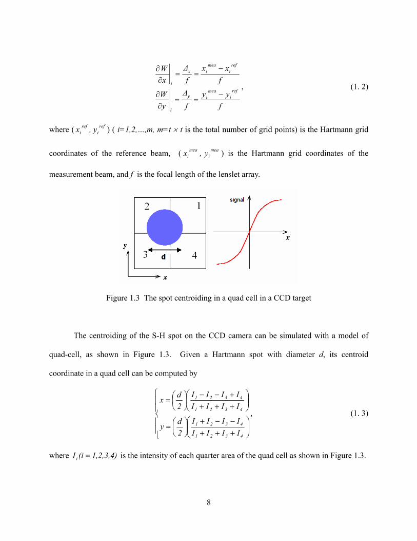
Figure 1.3 The spot centroiding in a quad cell in a CCD target

The centroiding of the S-H spot on the CCD camera can be simulated with a model of

quad-cell, as shown in Figure 1.3. Given a Hartmann spot with diameter d, its centroid

coordinate in a quad cell can be computed by

⎪⎪

⎩

⎪⎪

⎨

⎧

⎟⎟⎠

⎞⎜⎜⎝

⎛+++−−+

⎟⎠⎞

⎜⎝⎛=

⎟⎟⎠

⎞⎜⎜⎝

⎛++++−−

⎟⎠⎞

⎜⎝⎛=

4321

4321

4321

4321

IIIIIIII

2dy

IIIIIIII

2dx

, (1. 3)

where 1,2,3,4)(iI i = is the intensity of each quarter area of the quad cell as shown in Figure 1.3.

9

Figure 1.4 Quad cell in S-H WFS versus quadrant in pyramid WFS

(Adopted from Bauman)

A recent variation of the S-H sensor is the pyramid wavefront sensor (PWFS), which was

invented by R. Ragazzoni (Ragazzoni 1996).12, 13 A four-faceted pyramidal prism is used in the

nominal focal plane of the optical system to divide the focal image into four quadrants, which is

analogous to using a quad cell to divide a S-H spot in the CCD camera, except for the order

reverse of the optical element layouts between the two sensors (Bauman 2003).14 As shown in

Figure 1.4,14 the circle indicates the beam footprint on the wavefront sensor. For a S-H sensor

each sub-aperture on the CCD camera is a quad cell, while in a pyramid wavefront sensor each

pixel in each of the four pupils represents a quadrant of the quad cell. The pyramid wavefront

sensor uses a circular scan of the image to increase the measurement dynamic range, while in a

S-H sensor an increase of dynamic range can be achieved by employing a sub-aperture that is

larger than a quad cell to measure each S-H spot centroid. It was shown that the pyramid sensor

has a higher sensitivity with respect to a S-H sensor for the scenario of small wavefront

10

aberrations (Ragazzoni & Farinato 1999).15 However, fabricating the pyramidal prism for the

pyramid wavefront sensor has proven to be difficult.

1.1.3 Interferometric tests

Modern interferometry can be dated from the Michelson interferometer, which was

invented by Albert Abraham Michelson (1887).16,17 The classical interferometric tests in many

cases provide direct measurement of the optical path difference (OPD). Interferometry needs at

least two coherent wavefronts to interfere each other to generate an interferogram that records

the wavefront deformations. The two wavefronts could be either the reference wavefront and the

wavefront under test, or the wavefront under test and its duplicated wavefront with an offset

(shear).

For the first kind of interferometric tests, the reference wavefront is usually a perfectly

spherical or flat wavefront. The difference between the wavefront from the surface/system under

test and the reference wavefront is the wavefront OPD,1 which is a direct measure of the

wavefront error of the optical system under test. A perfect reference wavefront is quite important

for the first kind of interferometric tests, and the generation of a perfect reference wavefront is

difficult.

Shearing interferometry provides an alternate solution to this problem by using a copy of

the wavefront under test to replace the reference wavefront. The relative dimensions or

orientation of the reference wavefront must be changed (sheared) in some way with respect to

the wavefront under test.18 As such, an interferogram can be obtained from the interference of

the two sheared wavefronts. The most popular one is the lateral shearing interferometer, in which

11

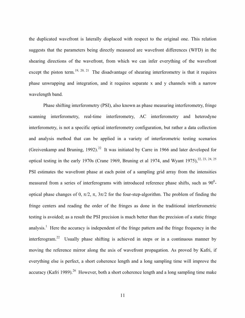
the duplicated wavefront is laterally displaced with respect to the original one. This relation

suggests that the parameters being directly measured are wavefront differences (WFD) in the

shearing directions of the wavefront, from which we can infer everything of the wavefront

except the piston term.19, 20, 21 The disadvantage of shearing interferometry is that it requires

phase unwrapping and integration, and it requires separate x and y channels with a narrow

wavelength band.

Phase shifting interferometry (PSI), also known as phase measuring interferometry, fringe

scanning interferometry, real-time interferometry, AC interferometry and heterodyne

interferometry, is not a specific optical interferometry configuration, but rather a data collection

and analysis method that can be applied in a variety of interferometric testing scenarios

(Greivenkamp and Bruning, 1992).22 It was initiated by Carre in 1966 and later developed for

optical testing in the early 1970s (Crane 1969, Bruning et al 1974, and Wyant 1975),22, 23, 24, 25

PSI estimates the wavefront phase at each point of a sampling grid array from the intensities

measured from a series of interferograms with introduced reference phase shifts, such as 900-

optical phase changes of 0, π/2, π, 3π/2 for the four-step-algorithm. The problem of finding the

fringe centers and reading the order of the fringes as done in the traditional interferometric

testing is avoided; as a result the PSI precision is much better than the precision of a static fringe

analysis.1 Here the accuracy is independent of the fringe pattern and the fringe frequency in the

interferogram.22 Usually phase shifting is achieved in steps or in a continuous manner by

moving the reference mirror along the axis of wavefront propagation. As proved by Kafri, if

everything else is perfect, a short coherence length and a long sampling time will improve the

accuracy (Kafri 1989).26 However, both a short coherence length and a long sampling time make

12

the interferometer more sensitive to mechanical vibrations and external changes. Therefore PSI

is not useful for testing systems in the presence of vibrations or turbulence.

It is to be noticed that the difficulty associated with the standard interferometric

measurements as well as the slope-based wavefront measurements, such as the S-H test, is their

sensitivity to rigid body rotations and displacements of the surface under test, and thus such

techniques are well-known to be vibration sensitive.

1.2 Recovery of the mid-spatial frequency: Modal or Zonal?

The shape of the wavefront error can be thought to be a combined contribution from the

errors of the following groups of spatial frequencies: the low spatial frequencies, which

contribute to the figure of wavefront; the mid-spatial frequencies, which contribute to the

“waviness” of wavefront; and the high spatial frequencies, which contribute to the roughness of

wavefront. 27,28 The low spatial frequencies characterize wavefront errors of less than 6 cycles

per aperture, the mid-spatial frequencies characterize wavefront errors of more than 6 cycles but

less than 20 cycles per aperture and the high-spatial frequencies characterize wavefront errors of

more than 20 cycles per aperture. Among them, the recovery of the wavefront mid-spatial

frequency errors is more interesting because it can help bringing the accuracy of wavefront

estimation to the next stage of the art, given that the low-spatial-frequency-based wavefront

estimations have been investigated extensively.

Wavefront errors can be quantitatively characterized by the power spectral density (PSD)

function of the wavefront, which is defined as the ensemble average of the squared modulus of

the wavefront function in the spatial domain.29 The PSD function quantifies the spectral power

13

of each spatial frequency in the pupil, which is actually a weight function for different spatial

frequency errors. As we will detail in Chapter 3, the wavefront values can be either evaluated at

each local point by zonal estimation or estimated as a set of orthogonal polynomials over the

whole test pupil by modal estimation. If a wavefront function is modal estimated with Zernike

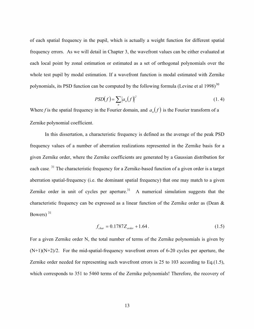
polynomials, its PSD function can be computed by the following formula (Levine et al 1998)30

( ) ( )∑=n

2n fafPSD (1. 4)

Where f is the spatial frequency in the Fourier domain, and ( )fan is the Fourier transform of a

Zernike polynomial coefficient.

In this dissertation, a characteristic frequency is defined as the average of the peak PSD

frequency values of a number of aberration realizations represented in the Zernike basis for a

given Zernike order, where the Zernike coefficients are generated by a Gaussian distribution for

each case. 31 The characteristic frequency for a Zernike-based function of a given order is a target

aberration spatial-frequency (i.e. the dominant spatial frequency) that one may match to a given

Zernike order in unit of cycles per aperture.31 A numerical simulation suggests that the

characteristic frequency can be expressed as a linear function of the Zernike order as (Dean &

Bowers) 31

64.11787.0 += orderchar Zf . (1.5)

For a given Zernike order N, the total number of terms of the Zernike polynomials is given by

(N+1)(N+2)/2. For the mid-spatial-frequency wavefront errors of 6-20 cycles per aperture, the

Zernike order needed for representing such wavefront errors is 25 to 103 according to Eq.(1.5),

which corresponds to 351 to 5460 terms of the Zernike polynomials! Therefore, the recovery of

14

the mid to high spatial frequencies with a modal approach becomes impractical given that such a

modal estimation requires solving for thousands of aberration basis coefficients.

Typically modal methods are good for the recovery of low spatial frequencies. One of the

advantages of the modal estimations is that the wavefront can be conveniently expressed as a set

of orthogonal polynomials, such as the Zernike polynomials, which individual term represents a

specific optical aberration. As a disadvantage, the orthogonality requirement of the Zernike

polynomials over the sampling geometry is a problem. Strictly speaking, the Zernike

polynomials are not orthogonal over a discrete set of sampling points inside a circular pupil, or a

pupil with central obscuration. Nevertheless, the tolerance on the pupil obscuration can be taken

up to thirty percent for example, without much effect on the Zernike coefficients. However, the

orthogonality of the Zernike polynomials can be seriously affected by the radial non-symmetry

of the pupil.

A higher-order modal decomposition can be thought to provide a better approximation to

the wavefront estimation, but this improvement is limited due to the fact that high frequencies or

‘‘spiky’’ phase data cannot be accurately represented by a Zernike basis (or any other basis) for a

fixed number of data values across the pupil. Dean & Bowers showed that for modal fitting of a

deformable mirror with Zernike polynomials, the Zernike order needs to go up to 50 (i.e.1326

terms!) for the RMS fit error to reaches λ/100 with a mid-spatial frequency wavefront error of 10

cycles/ aperture. 31

The alternate to modal estimation is zonal estimation, which is advantageous to move

wavefront estimation to the next level of accuracy. With zonal estimation, more sampling points

are also required for the retrieval of the mid-spatial frequencies. However, the slope/curvature

data sampling can be made as dense as needed without much computational burden for zonal

15

wavefront estimation, because the zonal method estimates the wavefront locally instead of

globally across the pupil in a modal method. For the zonal methods, the finite difference method

can be adopted for numerically solving a Poisson equation. With the finite difference method, a

wavefront value is a direct weighted average of its neighboring wavefront values corrected by

the increments gained from the neighboring slope measurements as we will detail in Chapter 3.

With curvature measurements, we will show in Chapter 6 that the zonal wavefront estimation

becomes very simple and elegant. Besides, there is no orthogonality requirement for zonal

wavefront estimation, thus any irregular pupil shapes may be considered as long as the boundary

conditions are satisfied. For these reasons mentioned above, we will focus on the zonal

wavefront estimation in this dissertation.

1.3 Vibrational effects

Mechanical vibrations (harmonic and nonharmonic) are often the principal source of

image degradation. 32, 33 Image motion or image blur caused by vibrations is common when the

imaging systems are located on a moving vehicle. Generally random vibrational motions are a

combination of many complex motions, including linear, quadratic and exponential motions, and

the intensity of each kind can be characterized by the power spectrum of the vibrations. In

airborne and terrestrial reconnaissance, astronomy, robotics, machine vision, and computer

vision systems, this motion degradation is generally much more severe than that from electronics

and optics.34

Vibrations degrade the image of optical systems, so does misalignment. They are often

the main error sources in optical testing, such as in a S-H sensor.35 The effect of misalignment

16

errors on the RMS wavefront error measured in a S-H sensor are detailed in a recent paper

(Curatu & Curatu and Rolland 2006).36

The impact of vibrations on optical testing is especially severe in the PSI technique, in

which the required data acquisitions at different phase steps make the PSI measurements more

vulnerable to vibration errors, and the accuracy of the PSI method is mainly restricted by the

vibrations during the measurements. 37 Various efforts have been made to depress the vibrations

and improve the measurement accuracy. The methods that have been proposed for suppressing

the vibrations include (1) taking the measurements fast enough to essentially freeze out

vibrations (Wizinowich 1990);38 (2) reducing the sensitivity of PSI to external vibrations by

simultaneously acquiring two complementary interferograms (Deck 1996);39 (3) using a filter-

based deconvolution to restore vibration-degraded video imagery (Barnard et al 1999);40 (4)

adopting longer sampling windows and higher frame rates (Ruiz et al 2001);41 (5) realizing the

required phase shift by quarter-wave plates and polarizers to avoid motion errors (Ngoi et al

2001);42 (6) using an active control loop to compensate for effects of vibrations (Zhao & Burge

2001); 43 (7) data postprocessing (Huntley 1998), 44 and (8) numerical optimization method

(Milman 2002).45

1.4 Motivation

Application requirements across various disciplines are always the original motivation to

move the technology of shape sensing forward. Questions fermented in applications for

wavefront testing technique include: How should one (1) handle the wavefront apertures that are

not round or square? (2) estimate wavefronts with a sampling geometry or methodology that has

17

the lowest noise propagation? (3) move wavefront testing to next level of accuracy? (4) recover

of the mid-spatial frequency error and (5) remove or reduce the effect of vibration and

misalignments?

In this dissertation, our research is focused on how to optimize wavefront estimation

with the above mentioned concerns. A zonal wavefront estimation algorithm without any

required apriori knowledge of the pupil shape is developed, which provides a solution for

wavefront estimation with irregular pupil shape. In order to reduce the wavefront estimation

error, the error propagations in wavefront estimation with different geometries are studied, and

the lowest error propagator for wavefront estimation is explored.

Considering a surface with a regular mesh, the slope measurement at each mesh location

is a linear approximation of the surface with a tangential plane, while the local curvature is a

quadratic approximation to the surface with an osculating quadric spherical surface.46 As a

consequence, the local curvature measurements are believed to yield a better recovery of the

mid-spatial-frequency errors than from the local gradient data.27 The principal curvatures and

their directions, which can be computed from the local Laplacian curvatures and the twist

curvature terms, provide a better characterization of wavefront local shape. In addition, a

curvature sensor as opposite to a slope sensor yields vibration-insensitive measurements. For

these reasons, a new sensor called differential Shack-Hartmann curvature sensor is proposed and

developed in this dissertation.

1.5 Dissertation outline

The remainder of the dissertation will be arranged as follow:

18

Chapter 2 summarizes the previous related work performed on curvature measurements,

which includes Roddier’s curvature sensor, the hybrid wavefront curvature sensor, and the

curvature profiling technique.

Chapter 3 reviews previous wavefront estimation techniques, which include wavefront

estimation algorithms from slope or curvature data based on the least-squares or Fourier

transform method. The wavefront phase retrievals from wavefront irradiance measurements are

also reviewed, which include the Gerchberg-Saxton method, Misell method, and phase diversity

techniques.

Chapter 4 describes a new least-squares-based wavefront estimation algorithm from slope

data for any irregular pupil shape. The mathematical framework for a pre-defined wavefront

estimation matrix without knowledge of the pupil shape is given, and examples for two different

pupil shapes are illustrated.

Chapter 5 quantitatively investigates error propagation in wavefront estimation. The

functions that depict the error propagation behavior for different estimation geometries are

established based on the matrix eigenvalue technique.

In Chapter 6, a new wavefront curvature sensor is proposed, called differential Shack-

Hartmann (DSH) curvature sensor. The algorithm for zonal wavefront estimation from curvature

measurements is given, and the mathematical framework for evaluating the principal curvatures

is presented.

Chapter 7 provides a validation of the proposed zonal curvature-based wavefront

estimation algorithm. An Error analysis of the experimental system for the DSH curvature

sensor is also given.

19

Chapter 8 summarizes the contributions of the research presented in this dissertation and

discusses future directions.

20

CHAPTER TWO: REVIEW OF CURVARTURE SENSING

In this chapter, we will focus on the popular quantitative wavefront sensors that are based

on measurement of wavefront curvature, the second derivative of wavefront. Wavefront

curvature is an intrinsic parameter of wavefront. Unlike the slopes (gradients or the first order

derivatives of shape), which vary with the surface orientation change, the surface normal

curvature is insensitive to tip/tilt or orientation change of the surface.

In this chapter, the curvature sensing techniques will be briefly reviewed, which include

Roddier’s wavefront curvature sensor, the Coherent Gradient Sensing method, a hybrid

wavefront curvature sensor, and the curvature profiling technique.

2.1 Roddier’s wavefront curvature sensor

Considering a surface with a regular mesh, and given two arbitrary but orthogonal

directions referred to the x- and y- directions, the local curvatures of the wavefront surface

)y,x(W along the x- and y- directions cx and cy are given by

⎪⎪⎩

⎪⎪⎨

⎧

∂∂

=

∂∂

=

2

2

y

2

2

x

yW(x,y)c

xW(x,y)c

, (2. 1)

and the Laplacian of the wavefront is defined by

2

2

2

22

yW(x,y)

xW(x,y)W(x,y)

∂∂

+∂

∂=∇ . (2. 2)

21

In 1988, Francois Roddier proposed a method to measure the local curvature of a

wavefront surface by measuring the difference in illumination at the two planes located before

and after the focal point (Roddier 1988).47 The principle of this sensor is illustrated in Figure

2.1.48 Later, this method was extended to wavefront sensing with an extended reference source

by comparing the Fourier transforms of two oppositely defocused images instead of measuring

the difference in illumination (Kupke, Roddier and Mickey 1998).49, 50

(a) Image space

(b) Object space

Figure 2.1 The illustration of Roddier’s curvature sensing (from Malacara)

22

2.1.1 Methodology evolution

In the early 1980s, Teaque’s (Teaque 1982, 1983) 51 , 52 and Steible’s (1984) 53 work

established how to retrieve phase information from a focused image and a defocused image

formed by a non-coherent imaging system. They showed that if a diffracting aperture is much

larger than the wavelength, a paraxial beam (monochromatic or incoherent) propagating along

the z-axis can be written as a differential equation as 48

0z

E(x,y,z)ik2E(x,y,z)k2E(x,y,z) 22 =∂

∂++∇ , (2. 3)

where k=2π/λ is the wave number. One solution to this equation is of the form

))(ikW(x,y;zexpI(x,y;z)E(x,y,z) 2/1= , (2. 4)

where I(x, y; z) is the distribution of the illumination at a location z along the beam, and W(x, y;

z) is the wavefront at a distance z from the origin. Substituting E(x,y,z) of Eq.(2.4) into Eq.(2.3),

and equating real and imaginary parts to zero separately, yields52

2

22

222 I

Ik81W

21I

Ik411

zW

∇−∇−∇+=∂∂ (2. 5)

and52

0WIWIzI 2 =∇+∇∇+∂∂ (2. 6)

where yx

xx

rr⋅

∂∂

+⋅∂∂

=∇ is the gradient operator. Eq.(2.5) is the wavefront transport equation,

and Eq.(2.6) is the irradiance transport equation. The WI∇∇ term in Eq.(2.6) is called the prism

term, representing the irradiance variation caused by a transverse shift of the beam due to the

local tilt of the wavefront, and the term WI 2∇ is called the lens term, which can be interpreted as

the irradiance variation caused by the convergence or divergence of the beam, whose local

23

curvature is proportional to W2∇ . Eq. (2.6) was originally derived for coherent light, but it is

also valid for an incoherent extended light source when the source is uniform and symmetric.53

Solutions to Eq.(2.6) are available. A Fourier transform-based phase retrieval method was

reported by Ichikawa et al (1988).54 Teaque (1983) provided a solution based on a Green’s

function, whose boundary value is constrained to be zero at the edge.54 By the use of the

Neumann boundary condition, another Green’s function-based solution was given by Woods and

Greenaway (2003).55

The irradiance transport equation shows that one can estimate the wavefront local

curvature by measuring the axial irradiance. If we assume that the illumination over the pupil

plane is uniformly equal to 0I ( 0I =∇ ) everywhere but at the pupil edge, we have the boundary

condition

c0II δ−=∇ n , (2. 7)

where cδ is a linear Dirac distribution around the pupil edge, and n is a unit vector perpendicular

to the edge and pointing outward.

Combining Eq.(2.6) and Eq.(2.7) yields (Roddier 1990)56

WPIδWIzI 2

0c0 ∇−∂∂

=∂∂

n (2. 8)

where W/W ∇⋅=∂∂ nn , and P(x, y) is defined as the pupil function, whose value is one inside

the pupil and zero outside. The irradiances at two defocused pupil images are given as

⎪⎪⎩

⎪⎪⎨

⎧

Δ∂∂

−=

Δ∂∂

+=

zzIII

zzIII

02

01

(2. 9)

Therefore,

24

zzI

I1

IIII

021

21 Δ∂∂

=+− (2. 10)

By combining Eq.(2.10) with Eq.(2.8), Roddier obtained

zWPWIIII 2

c21

21 Δ⎟⎠⎞

⎜⎝⎛ ∇−δ∂∂

=+−

n, (2. 11)

where zΔ is the distance from the pupil plane to the defocused plane P1 or P2 viewed from the

object space. A plane at a distance zΔ from the pupil can be Fourier transformed to a plane at a

distance from the focus. Roddier proved that (1993)57

ll)f(fz −

=Δ , (2. 12)

where f is the system focal length and l is the defocus distance of the defocused plane. Then he

obtained the well-known equation for curvature sensing given by

⎟⎠⎞

⎜⎝⎛ ∇−δ∂∂−

=+− WPW

ll)f(f

IIII 2

c21

21

n. (2. 13a)

Specifically,

⎥⎥⎥⎥

⎦

⎤

⎢⎢⎢⎢

⎣

⎡

∇−δ∂

⎟⎠⎞

⎜⎝⎛∂

−=

−+−−

)lf(WPl

fW

ll)f(f

)(I)(I)(I)(I 2

c21

21 rn

r

rrrr r

r

rr

rr

(2.13b)

As pointed by D. Malacara et al., the operations on the irradiances in the two measured

images must correspond to the same point on the pupil plane (Malacara 1998).48 As such, one of

the defocused image is rotated 1800 with respect to the other. The above derivation is based on

geometrical approximation, which is valid only when the irradiance measurements are made

close to the pupil. 47, 58 Chanan obtained an equation that is the same as Eq.(2.11) by making an

25

integration on the focal plane based on the method of stationary phase provided by Born & Wolf

(Chanan 2000).59, 60

2.1.2 Implementations

In principle, the two out-of-focus images should be measured simultaneously, or within a

time interval much shorter than the expected wavefront evolution time. In optical testing

applications, this time constant is determined by the vibrational environment that is to be

overcome. One implementation of curvature sensing is to employ two beam splitter prisms and

one right angle prism to separate out the two extra-focal images and direct them on one detector

array.61 The advantage of this approach is that both images are detected at the same time, and this

approach involves no moving parts, therefore it is very stable. This approach may suffer,

however, from chromatic and geometric aberrations (spherical and astigmatism) introduced by

prisms if it is not properly configured.

Another implementation is to employ a variable curvature membrane mirror driven

acoustically at 7 kHz to switch between the re-imaging of the two defocused beam cross sections

onto a detector. 62, 63 This oscillating membrane is located at the focus of the optical transfer

lens. When the membrane mirror is flat, the light reflected from this mirror will re-image the

telescope pupil onto the detector; when the mirror is inflated, the pupil image will be defocused

on the detector in either direction. Because the distance to the focus changes continuously as the

membrane vibrates, a stroboscopic technique or a fiber-optic LED transmitter is used to freeze

the position of the mirror when the membrane vibrates back and forth. In one cycle of the

membrane oscillation, the detector needs to record both intra focal and extra focal distributions

26

of the light beam. This process usually makes the system quite noisy, and to-date this

implementation has not been very successful.

Besides the above configurations, Ervin Goldfain proposed a curvature sensor with a

single-detector/single-image setup with partially coherent light (Goldfain 1998),64 in which the

twin images were computed from the mutual intensity in the paraxial image plane according to

the propagation laws of mutual intensity along the optical axis.

2.1.3 Advantages and disadvantages

The advantage of the curvature sensing method given by Roddier is its opto-mechanical

simplicity and the fact that no lenslet arrays or re-imaging systems are needed. Also the

sensitivity of the curvature sensor is comparable to that of the S-H test,58, 65 and it can be

changed continuously by varying the defocus distance l. The most impressive advantage of such

a curvature sensor is that the signal from the curvature sensor can be amplified and directly

applied to the mirror actuator in a deformable mirror system without any wavefront estimation

process.66

The potential disadvantage of Roddier’s curvature sensing method as it is applied to

optical testing is the error propagation in the wavefront estimation algorithm (Roddier 1990).56

Its performance is limited not only by the quality of the detector used for irradiance

measurements but also by the separation between measurement planes used for the calculation of

the axial derivative of intensity (Soto, Acosta & Ríos 2003).67 From the finite difference point of

view, if the separation between measurement planes is small, the axial derivative should be more

precise, but the spatial resolution of the sampling is low. On the other hand, if the distance

27

between the planes is large, the spatial resolution of the sampling will be increased, but the

calculation of the derivative is less precise. Therefore, there exists an optimum separation

distance between the intensity measurement planes.

The determination of the defocus distance is also affected by seeing blur and the caustic

zone. The defocus image diameter should be twice as large of the seeing blur, and the defocused

image planes should be taken outside the caustic zone, because inside the caustic zone the rays

coming from different sample pupil points intersect.57 Unfortunately the size of the caustic zone

depends on the aberrations of the optics under test, and the evaluation of an optimum position for

the defocused measurement planes depends on the apriori knowledge of the phase to be

measured. Besides the difficulty in determining the defocused distance, the exact position of the

optical focus can be hard to determine, especially for slow f-ratios. Therefore, the distances of

the measurement interfaces to the focus and their sizes may not be identical. As discussed above,

how to determine the twin measurement interfaces is critical to the proper operation of Roddier’s

curvature sensor. In 2003 a formula was presented by Soto et al. for determining the ideal

defocused measurement planes when only a minimum knowledge of the phase is available.67 In

2003, a derivative of Roddier’s curvature sensor, which consists in directly measuring the

Zernike components of an aberrated wavefront, was introduced (Neil, Booth &Wilson 2000).

68,69

2.2 Special wavefront curvature sensors

In this section, we briefly review other special curvature sensing techniques, the Coherent

Gradient Sensing method and a hybrid technique for wavefront curvature sensing.

28

2.2.1 CGS wavefront curvature sensor

Coherent Gradient Sensing (CGS) is a diffraction-based, full-field, real-time, wavefront

sensing approach for measuring wavefront curvature (Tippur 1992).70 CGS is especially useful

for measuring curvatures of micro-mechanical structures and thin films in electronic devices and

for studying the properties of materials and the stress distribution. CGS yields curvature data

over the entire surface area of interest and it is insensitive to rotation or displacement of the

object under test. A reflection-mode CGS setup is shown schematically in Figure (2.2).71 The

coherent collimated laser beam is directed to the surface under test and reflected. The beam then

passes through two identical Ronchi gratings (40 lines/mm) separated by a distance Δ, and the

interference between two wavefronts sheared in a distance ω takes place. A lens is used to

image the wavefront fringes on the image plan, while focusing the diffracted light to form

distinct diffraction spots on a filter plane. A filtering aperture is used in the filter plane to select a

diffraction order of interest and block the other orders. A video camera is used to receive the

fringe map, which is a contour plot of the wavefront gradient field. The video image is digitized

and processed to extract information on the curvature of the surface under test.

If the Ronchi grating lines are oriented along the x1 axis, the working principle of the

CSG curvature sensor is illustrated in Figure 2.3.72 The incident beam on the primary grating G1

is diffracted into several wavefronts denoted as E0, E1, E-1, E2, E-2, etc, which are further

diffracted by grating G2. Various sets of parallel diffracted beams are combined by the filtering

lens to form diffraction spots D1, D0, and D-1, etc. An aperture pupil is placed on the filter plane

to select the order of interest.

29

Figure 2.2 Schematic for a reflection CGS curvature sensor (Adopted from Kolawa)

The constructive interference maybe expressed as72

L,2,1,0n ,λn)x,xW()x,xW( (2)(2)2121 ±±==−ω+ (2. 14)

where )( 2n represents the integer identifying fringes observed for shearing along the x2 direction.

And Δ= θω , where Δ is the interval between two gratings; p/λ=θ is small, where p is the

grating period. For sufficiently smallω , the authors obtained

L,2,1,0n ,pnn)x,xW()x,xW(x

)x,xW( )2()2()2(

2121

2

21 ±±=Δ

=ωλ

=ω−ω+

=∂

∂ (2. 15)

30

Figure 2.3 The principle of a CSG curvature sensor (from Kolawa, et al)

This equation shows that the wavefront slopes in the 2x direction are obtained. By

rotating the two gratings in 090 , we can obtain the wavefront slopes in 1x direction. Generally,

in the 1x or 2x directions, we have

.1,2 and ,2,1,0n ,pnx

)x,xW( )()(

21 =α±±=Δ

=∂

∂ αα

α

L (2. 16)

A detailed Fourier optics analysis proved that the image plane of a CGS sensor is a

gradient field of the wavefront under test70, from which the curvature information can be

extracted by a finite difference method. For small curvatures, 1W2 <<∇ , a curvature tensor αβκ

along the unit tangent vectors a1 and a2 can be approximated as 70

( ) ( ) .1,2, . ,2,1,0n ,x

)x,x(npxx

x,xWx,x )(21

)(21

2

21 =βα±±=⎟⎟⎠

⎞⎜⎜⎝

⎛

∂∂

Δ≈

∂∂∂

≈κ α

β

α

βααβ L (2. 17)

31

where αβκ is the symmetric curvature tensor, whose component 11κ and 22κ are termed as normal

curvatures, and 2112 κκ = as twist curvature terms.

2.2.2 Hybrid wavefront curvature sensor

The hybrid wavefront curvature sensor to be described here measures the curvatures and

gradients of the wavefront using a configuration that resembles a Shack–Hartmann sensor

(Paterson & Dainty 2000).73 An array of astigmatic lenslets is used to generate an array of foci

on a single detector plane. The shape of each focused spot is related to the local wavefront

curvature as shown in Figure 2.4,73 and a quad-cell detector is used to measure each spot.

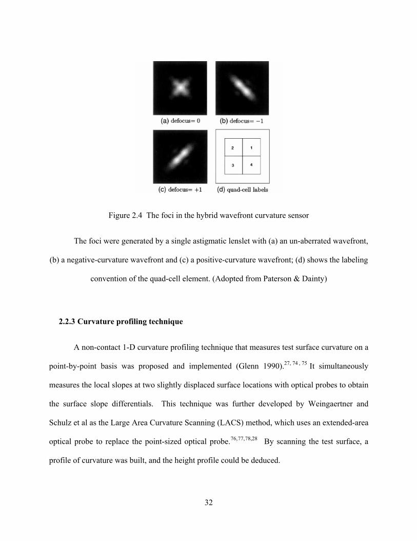
When a parallel wavefront (i.e. there is no wavefront curvature) is incident on a lenslet,

the focus is shown in Figure (2.4a). If the incident wavefront has curvature, the balance between

the two diagonal cells is broken. The normalized difference between the sums of the signal

intensities from diagonal elements of the quad cell yields an estimation of the local wavefront

Laplacian, which is given as

4321

4321c ssss

sssss+++−+−

= . (2. 18)

The normalized difference between the right and left half (or upper and lower) of the quad cell

yields a measure of the wavefront gradient given by

⎪⎪⎩

⎪⎪⎨

⎧

++++−−

=

+++−−+

=

4321

4321y

4321

4321x

sssssssss

sssssssss

. (2. 19)

32

Figure 2.4 The foci in the hybrid wavefront curvature sensor

The foci were generated by a single astigmatic lenslet with (a) an un-aberrated wavefront,

(b) a negative-curvature wavefront and (c) a positive-curvature wavefront; (d) shows the labeling

convention of the quad-cell element. (Adopted from Paterson & Dainty)

2.2.3 Curvature profiling technique

A non-contact 1-D curvature profiling technique that measures test surface curvature on a

point-by-point basis was proposed and implemented (Glenn 1990).27, 74 , 75 It simultaneously

measures the local slopes at two slightly displaced surface locations with optical probes to obtain

the surface slope differentials. This technique was further developed by Weingaertner and

Schulz et al as the Large Area Curvature Scanning (LACS) method, which uses an extended-area

optical probe to replace the point-sized optical probe.76,77,78,28 By scanning the test surface, a

profile of curvature was built, and the height profile could be deduced.

33

Figure 2.5 The differential measurement of slope

(Adopted from Glenn)

The optical schematic for the differential measurement of slope is shown in Figure 2.5.27

A calcite plate was used to produce two parallel beams with opposite linear polarization, and a

polarizing beam splitter was placed in the reflected path from the test piece to separate the two

measurement beams before they were focused by the collimation lens onto two separate

detectors. The “zero” curvature positions on the two detectors could be calibrated before hand,

and the difference between sensed positions on the detectors, which is proportional to the

difference of the test piece slopes at the two measurement locations, were used to calculate the

curvature at each test point. The schematic layout of the curvature profiling instrument is shown

in Figure 2.6,27 where the steering mirror is used for scanning the test surface, and the movable

detector is used to accommodate the focused spots on the centers of the two detectors.

34

Figure 2.6 Schematic layout of the curvature profiling instrument

(Adopted from Glenn)

The curvature profiling instrument measures the mid-frequency surface errors, whose

spatial periods span from a fraction of a millimeter to a hundred or more millimeters.27

Curvature is an intrinsic property of the test piece which is independent of its position and

angular orientation, and such property makes this approach fundamentally insensitive to all types

of vibration and drift in both surface height and surface slope. It is a self-reference test where no

reference surface is needed. The slope detectors can be two dimensional in order to measure both

the normal curvature (longitudinal or lateral) and the twist curvature term.

The disadvantages of this approach are listed below. (1) It is a one-dimensional point-by-

point measurement, which limits the temporal working bandwidth. (2) To reach the highest

performance, it is necessary to calibrate the steering mirror intrinsic curvature and the calcite

residual power, which is a complex problem since the steering mirror rotates in two dimensions.

(3) This approach measures the curvature of the test surface only, which corresponds to the mid-

spatial frequency errors, and it loses the information about the low spatial frequency errors, such

as spherical aberration and astigmatism. This technique demonstrates sub-angstrom accuracy and

35

λ/1000 sensitivity with the differential distance of 0.3mm and a sample spacing of 10 μm on a

test piece of 10mm.74

2.3 Summary

Curvature is intrinsic and absolute parameter of wavefront and the curvature

measurements is usually vibration insensitive. In this chapter, we reviewed four curvature

sensing techniques, the Roddier curvature sensor, the CGS wavefront curvature sensor, a hybrid

curvature sensor, and a 1-D curvature profiling technique. Of all these sensors the 1-D curvature

profiling technique measures the second derivatives only, Roddier’s curvature measurements

include both wavefront Laplacian inside the pupil and wavefront gradient around the boundary,

and the others measure both the second derivatives and the first derivatives of the wavefront.

Currently Roddier’s curvature sensor is mainly applied in astronomy for adaptive optics system

to take the advantage of the analog nature of its sensor signal to the deformation of the

deformable mirror. The curvature profiling technique is used as a unique instrument in

profilometry which is immune to vibrations. So far the CGS and the hybrid wavefront curvature

sensors have not been widely used in applications. More features of curvature sensing will be

explored as a new wavefront curvature is proposed and implemented in Chapter 6.

36

CHAPTER THREE: REVIEW OF WAVEFRONT ESTIMATION TECHNIQUES

In this chapter, we will first review wavefront estimation techniques that are based on

wavefront parameter measurements, specifically the first and second derivative measurements

(i.e. wavefront slope (gradient) and curvature measurements). Wavefront estimation converts the

wavefront parameter measurements into wavefront OPD, or wavefront phase by multiplying the

OPD by the optical wave number 2π/λ. Mathematically it is a Neumann boundary problem of

Poisson’s equation. 11

The wavefront phase retrieval methods that are based on the irradiance measurements are

also reviewed. The phase retrieval methods include Gerchberg-Saxton and Misell methods, and

the phase diversity technique, all of which employ phase deconvolution algorithms with iterative

Fourier transform operations. The phase retrieval algorithms are usually computational intensive.

3.1 Neumann boundary problem in wavefront estimation

Consider that the measured gradient function of a wavefront is ( )y,xg , which includes the

real wavefront gradient W∇ and the random additive measurement noise ( )y,xn , i.e.

( ) ( ) ( )y,xy,xWy,x ng +∇= , (3.1)

where W is the wavefront under estimation, and ∇ is the gradient operator. In a least-squares

sense, the task of wavefront estimation is to find a wavefront ( )y,xW that minimizes the

difference between W∇ and ( )yx,g , which is equivalent to minimize the functional integral

37

( ) ( )[ ]∫∫Ω

−∇= dxdyyx,y,xWJ 2g , (3.2)

where Ω is the wavefront testing area, either a composite field or a simply connected field, in

2ℜ with boundary i

n

1i0 CC U

=

+=Ω∂ and closure Ω∪Ω∂=Ω as shown in Figure 3.1. In the

following part we will show that wavefront estimation is a functional extremum problem in the

calculus of variations.60

Figure 3.1 The testing aperture for wavefront estimation

Let ( )Ω2C denote the space of all functions ℜ→Ω:W , such that W has continuous

derivatives of second order, and let’s define a functional

( ) ( ) ( )[ ] ( )[ ]2yx2

yx yx,yWxWyx,yx,W,WWy,x,F gg −+=−∇=rr , (3.3)

where xWWx ∂∂= , and yWWy ∂∂= . If F is a smooth function of x, y, xW and yW , then the

functional integral becomes ( ) ℜ→Ω2C:J with the form

( )[ ] ( )dxdyW,Wy,x,Fyx,WJ yx∫∫Ω

= . (3.4)

For the slope or Laplacian curvature-based wavefront estimations, the Neumann

boundary conditions should be satisfied. Therefore, the permissible function set for the solutions

to this problem is

38

( )⎭⎬⎫

⎩⎨⎧

=∂∂

∈=∂

x,yW),Ω(CWWS 0Ω

2 gn

. (3.5)

To obtain an extremum for the function ( )[ ]yx,WJ in Eq. (3.4), the Euler-Lagrange equation

should be satisfied,79 i.e.

0WF

yWF

x yx

=⎟⎟⎠

⎞⎜⎜⎝

⎛

∂∂

∂∂

+⎟⎟⎠

⎞⎜⎜⎝

⎛∂∂

∂∂ . (3.6)

Applying Equation (3.3) in Equation (3.6) yields

yy

xxy

WxW

2

2

2

2 rv

∂∂

+∂∂

=∂∂

+∂∂ gg , (3.7)

or

( ) ( )x,yfx,yW2 =⋅∇=∇ g , (3.8)

which is a Poisson equation. The wavefront estimation problem can then be described as a

Neumann boundary problem of the Poisson’s equation stated as 11

( )

( ) ( ) Ωx,y yx,W

yx,fW

0Ω

2

0

∈⎪⎩

⎪⎨

⎧

=

=∇

gn ∂∂

∂ . (3.9)

We have supposed that the wavefront function W has at least second order derivatives

that are continuous on a closed regionΩ , so the solution to the Neumann boundary problem

exists and is unique, except for an additive constant.

As implied by Eq.(3.9), we can estimate the wavefront by measuring either the wavefront

gradient ( )yx,g or wavefront curvature ( )yx,f , but it is difficult to find an analytic solution for

this problem, so a numerical solution is sought in practice. By employing a finite difference

method, the wavefront testing domain can be discretized into a regular mesh grid. We can either

39

evaluate the wavefront value at each local point that best fits the measurement data (i.e. the zonal

wavefront estimation) or evaluate the estimated wavefront as a set of orthogonal polynomials

over the whole pupil under test (i.e. the wavefront modal estimation).

3.2 Slope-based wavefront estimations

As we discussed in Chapter 1, a zonal estimation is advantageous in mid-spatial

frequency recovery, and it is also convenient for accommodating irregular pupil shapes.

Basically, there are three sampling geometries available for wavefront estimation from slope

data: the Hudgin geometry, the Southwell geometry, and the Fried geometry as shown in

Figure 3.2, where the small circles symbolize the wavefront values and the small arrows are

wavefront slope measurements in the x- and y-directions.

Figure 3.2 Sampling geometries for wavefront estimation

(1) Hudgin geometry (2) Southwell geometry (3) Fried geometry.

In recent literature, Hudgin was published as Hutchins

40

3.2.1 Zonal slope-based wavefront estimation

The zonal slope-based wavefront estimation can be performed either by a least-squares

fitting method or by a Fourier transform method. The zonal least-squares estimation is usually a

numerical solution to Poisson’s equation with the finite difference method. The Poisson’s

equation can be expressed by a system of difference equations defined on the sampling grid.

Since a partial derivative is an ordinary derivative taken with respect to one variable while the

other variable is held fixed, we can write

( ) ( ) ( ) ( )2

j1ijij1iji2

2

a,yxW,yxW2,yxW

,yxxW +− +−

≈∂∂ , (3.10)

where a is the grid interval. Similarly for the y-derivative we can write,

( ) ( ) ( ) ( )2

1jiji1jiji2

2

a,yxW,yxW2,yxW

,yxyW +− +−

≈∂∂ . (3.11)

Figure 3.3 Five-point stencil

41

Substituting Eqs.(3.10) and (3.11) into Eq.(3.9), we obtain a discretization approximation

to Poisson’s equation with an precision order of ( )2aO ,

( ) ( ) ( ) ( ) ( ) ( )ji2

j1i1jiji1jij1i y,xfay,xWy,xWy,xW4y,xWy,xW =++−+ ++−− . (3.12)

Each equation involves five unknown wavefront values, whose relative locations

represent the weights with which the five unknowns are combined as shown in Figure 3.3. This

geometry is called the five-point stencil in the finite difference method, which can be used for

approximating the Poisson’s equation.11, 80 The right side of this equation is wavefront curvature,

which can either be obtained from direct measurements or numerically estimated from the slope

measurements.

Fourier transforms of the slopes of a wavefront, for example in the x-direction, can be

given as

( ) ( ) ( ) y,xWFT2iξx

y,xWFT ⋅πξ=⎭⎬⎫

⎩⎨⎧

∂∂ , (3.13)

where ξ is the spatial frequency associated to the x-dimension. Similarly, we can obtain the

Fourier transform of slopes in the y-direction as

( ) ( ) ( ) y,xWFT2iyx,yWFT ⋅πη=η

⎭⎬⎫

⎩⎨⎧

∂∂ , (3.14)

where η is the spatial frequency associated with the y-dimension. We then obtain the Fourier

transform-based formula for wavefront estimation from slope data as48

( )

( ) ( )

⎪⎪⎭

⎪⎪⎬

⎫

⎪⎪⎩

⎪⎪⎨

⎧

η+

⎥⎦

⎤⎢⎣

⎡∂

∂⋅η+⎥⎦

⎤⎢⎣⎡

∂∂

⋅ξ⋅

π−= −

221

ξyx,yWFT

xx,yWFT

FT2ix,yW . (3.15)

42

3.2.1.1 Least-squares fitting method

The zonal wavefront estimation technique can be traced back to 1974 when Rimmer

formulated to estimate the wavefront from static shearing interferograms sampled on a

rectangular array of points (Rimmer 1974).81 The estimation geometry Rimmer adopted was

actually known later on as the so-called Hudgin geometry (Hudgin 1977), 82 in which the

wavefronts are evaluated at each grid points while the WFDs are measured between two

neighboring grid points. The wavefront estimation matrix was established using a least-squares

fitting method. An iterative relaxation method was employed to solve this equation. With the

Hudgin geometry, a real-time wavefront reconstructor for adaptive optics was built (Hardy,

Lefebvre & Koliopoulos 1977).83 J. Wyant showed that the wavefront measurement accuracy of

this geometry depends only on the radiance of the shearing light source and not upon the angular

subtense of the source (Wyant 1975).84

For the Fried geometry, the wavefront value at each grid point is evaluated while the

slopes (or WFDs) at the center of each grid cell are measured (Fried 1977). 85 The slope data

between each pair of neighboring grid points is estimated as an average of two slope data at the

centers of the two neighboring grid cells. Given a generalized square array of the sampling grid,

Hunt formulated the wavefront estimation matrix equation for the Hudgin and Fried geometries

(Hunt 1979).86 Hunt, Hudgin and Fried all found that the error propagation in the estimation

shared the form of β+α )Nln( , where N is the number of the sampling grid size, and α and β

are constants that depend on the sampling geometry adopted . Noll revealed that the logarithmic

behavior of the error is a fundamental property of the Green’s function for a Neumann boundary

problem of a Poisson’s equation, and that the offset of the results from Hudgin and Fried is

43

caused by neglecting the contribution from the boundary condition (Noll 1978).87 We will show

in Chapter 5 that parity of the sampling array dimension also contributes to the error propagation

in wavefront estimation.

The Southwell geometry is characterized by taking the wavefront slope measurements

and wavefront values estimation at the same nodes (Southwell 1980).88 The wavefront slope

data at the midpoint between each pair of neighboring points is estimated as an average of the

slope data at these two neighboring points. Southwell formulated the error propagation for zonal

wavefront estimation and showed its superiority over other geometries. However, Wallner

formulated a different opinion regarding the performance between different wavefront estimation

geometries (Wallner 1983). 89 In Chapter 5, we will discuss error propagation for different

wavefront estimation geometries in detail.

Hudgin82, Hardy et al,83 Fried, 85 Hunt,86 Southwell88, and Su et al 90 all showed that a

least-squares based estimation scheme of a wavefront value iW can be expressed as

)dcbaDCBA)(G/1(Wi +−−++++= , (3.16)

where A, B, C and D are the wavefront values at the four adjacent nodes of iW ; a, b, c and d are

the adjacent WFDs between iW and its adjacent nodes. G will be 4 if iW is an interior node, and

3 and 2 if iW is an edge or corner node, respectively. The wavefront inside the pupil is the

average of its four nearest neighbors plus the average of the four connecting WFDs with the

appropriate signs in the WFDs. This is actually the discretized approximation of Poisson’s

equation, a general form for slope-based least-squares wavefront estimation.

Herrmann formulated the matrix equations for wavefront estimation for Hudgin and Fried

geometries and showed that the ranks of the estimation matrices for the two geometries are m-1

44

and m-2, respectively (Herrmann 1980), 91 where m is the total number of wavefront grid points.

Since the estimation matrix is rank-deficient, Herrmann suggested using singular value

decomposition (SVD) to obtain the Moore-Penrose inverse of the estimation matrix, which is a

least-squares solution with the minimum norm (LSMN). Besides the LSMN solution, he

suggested to set a “zero point” for the wavefront to make the estimation matrices full-rank, at

which the wavefront value is assigned to zero or other constant. Herrmann’s method of

evaluating the LSMN solution by forcing the wavefront mean value to be zero is limited, because

a wavefront that has a minimum norm does not necessarily have a zero mean value.

The Fried geometry perfectly matches with the lenslet array of the S-H sensor and

actuator array of a deformable mirror, yielding currently the most popular configuration in

adaptive optics. But wavefront estimation with the Fried geometry suffers from waffle mode (or

checkerboard mode), which will be further detailed in Chapter 5.

3.2.1.2 Fourier transform method

A Fourier transform-based algorithm for wavefront estimation from slopes was proposed

(Roddier & Roddier 1991).92 In order to remove the boundary effect in the Fourier transform

process due to the limited size and shape of the pupil function, Gerchberg-Saxton iterations were

used to extrapolate the fringes outside of the test pupil (Roddier & Roddier 1987). 93 The

Gerchberg-Saxton algorithm is an iterative irradiance-based wavefront estimation method that is

widely used in phase retrieval, which will be further detailed in Section 3.4. The flow chart of

the Gerchberg’s fringe extrapolation algorithm is illustrated in Figures 3.4, and Figure 3.5 shows

a comparison between the interferograms before and after the extrapolation of the fringes. Based

45

on Gerchberg’s extrapolation, an iterative Fourier transform-based wavefront estimation from

slope data can be performed, whose flow chart is illustrated in Figure 3.6.

Figure 3.4 The flow chart of Gerchberg’s fringe extrapolation algorithm.

(from Roddier & Roddier 1987)

(a) (b)

Figure 3.5 An example of interferogram extrapolation (from Roddier & Roddier1987)

(a) Interferogram before fringe extrapolation (b) Interferogram after fringe extrapolation

46

Figure 3.6 Flow Chart for the iterative FT-based wavefront estimation from slope data

(from Roddier & Roddier 1991)

3.2.2 Modal slope-based wavefront estimation

In modal estimation, a wavefront is decomposed into a linear combination of whole-

aperture basis functions, such as Zernike polynomials, 94 Karhunen-Loeve functions, 95 , 96 , 97

Legendre polynomials,88 Fourier Series,98 etc. Thus a wavefront can be expressed as

( ) ( )y,xZay,xW k

M

0kk∑

=

= (3.17)

where ka are the coefficients to be determined, and ( )y,xZ k are two-dimensional functions that

are orthogonal over the discretely sampled aperture. The Zernike circle polynomials are such a

47

set of orthogonal functions over a unit circle, which was first introduced by Zernike (Zernike

1934)99 and was later studied by Brinkman, Nijber, Bhatia and Wolf, Mahajan, et al.60 In a polar

system, the modified Zernike circle polynomials given by Noll can be written as94, 100, 101, 102.

( )( ) ( )( ) ( )

( )⎪⎩

⎪⎨

⎧

=ρ+≠ρ+≠ρ+

=ρ0m ,R1)(n

0m odd, k θmsinR1)2(n0m even, k θmcosR1)2(n

θ,Zmn

mn

mn

k , (3.18)

where 10 ≤ρ≤ and π≤θ≤ 20 . The radial degree n and the azimuthal frequency m should

satisfy nm ≤ and nm − even. The index k=1, 2, 3… is a mode ordering number, and

( ) m/2mnnk ++= . Born and Wolf showed that 60

( ) [ ] [ ]∑−

=

−ρ−−−+

−−=ρ

m)/2(n

0s

2sns

mn !sm)/2(n!sm)/2(n!s

!s)(n1)(R . (3.19)

Therefore the modified Zernike polynomial can be written in the following form

( ) ( )( ) ( ) ...3sin83cos8cos238sin238

2sin62cos6123sin2 cos21,Z3333

222k

θρ+θρ+θρ−ρ+θρ−ρ+

θρ+θρ+−ρ+θρ+θρ+=θρ (3.20)

According to Mahajan, the Zernike circular polynomials (3.18) can be written in a

simpler form as 103,104,105

( ) ( ) ( ) ( )θimexpρR1nθ,Z mn

2/1k +=ρ . (3.21)

The orthogonality of the Zernike polynomials means that the inner product of any Zernike

polynomials is zero when the inner product is performed over a unit circle, which is94

( ) ( ) kll

1

0

2

0 k dd,Z,Z1δ=θρρθρθρ

π∗π

∫ ∫ , (3.22)

where klδ is zero for lk ≠ and 1 for lk = .

48

The merit of the Zernike polynomials is that each term represents a specific wavefront

aberration. For example, the constant 1 represents the piston error, terms θρ sin and θρcos are

wavefront tip/tilt, and term θρ 2sin2 and θρ 2cos2 are astigmatism, etc. Furthermore, the

Zernike polynomials are orthogonal to each other over a unitary (i.e. normalized to 1) circular

pupil without central obscuration. Then the variance of the wavefront is given by the sum of the

squared aberration coefficients.106

3.2.2.3 Least-squares based modal estimation

If a wavefront is given by Eq. (3.17), then the derivatives of the wavefront are given by

( ) ( )yx,Zayx,W k

M

1kk∇=∇ ∑

=

. (3.23)

By matching the gradient data measured in wavefront sensing at each discrete node

( )TN1 ggG L= , where 1,2,...N,iyWy

xWx

iii =

∂∂

+∂∂

=rrg , we have a matrix equation

GDA = , (3.24)

where D is the gradient matrix, and ( )TM1 aa L=A is the coefficient vector to be

determined. In the least-squares sense, both Cubalchini (1979) 107 and Jan Herrmann (1981)

derived the corresponding normal equation as108

GDDAD TT = . (3.25)

If matrix D has its full column rank, then the least-squares solution is 109

GDD)(DA T1T −= (3.26)

49

The Zernike polynomials are orthogonal only on a unit disk. They are not orthogonal

over an irregular shaped pupil, such as a pupil with a central obscuration which is a common

case for an astronomical telescope. Furthermore, the Zernike polynomials are not strictly

orthogonal over discrete points in a unit circle disk, and all of the derivatives of the Zernike

polynomials are not orthogonal. Therefore, it is not proper to estimate the mode coefficients

directly from the slope data or curvature data by least-squares estimations.

Cubalchini studied the effect of cross correlation between the modal estimates as a result

of the non-orthogonality of the derivatives of the Zernike polynomials (Cubalchini 1979). He

showed that the modal estimation is sensitive to the number of slope measurements used and

their sampling geometry adopted. Although the set of basis functions needs not to be necessarily

orthogonal to each other, they should be independent (Hardy 1998).110 Jan Herrmann further

pointed out that the aberration cross coupling problem, caused by the lack of linear independence

of the column vectors of the matrix D, can be avoided if a least-squares estimate is performed

with an increased number of modes (Hermann 1981).108 To make a polynomial orthogonal, a

process called Gram-Schmidt orthogonalization can be employed (Wang and Silva 1980)100.

With the Gram-Schmidt orthogonalization, the Zernike orthogonal polynomials over circular

apertures can be extended to an annular aperture,103, 104, 105 or an hexagonal aperture,111,112 or

other general-shape apertures.113

Gavrielides first proposed to construct polynomials that are orthogonal to the gradient of

the Zernike polynomials for modal estimation (Gavrielides 1982).114 Given that the constructed

polynomials ( )θρ∗ ,lV and the gradient of the Zernike polynomials ( )θρ∇ ,Zk are orthogonal to

each other, their inner product satisfies

50

( ) ( ) kl*lk ρ,θρ,θZ δ=⋅∇ V . (3.27)

If the gradient data measured is ( )ρ,θG , then the Zernike coefficients can be computed by ( ) ( )ρ,θρ,θa kk

∗⋅= VG . (3.28)

The constructed polynomials ( )ρ,θkV were given by an integral of a product of the

gradient of a Green function defined on the unit circle and a Zernike polynomial. 114

Alternate to Gavrielides’ method, Acosta et al proposed to introduce an auxiliary vector

function ( )rkF whose gradient is orthogonal to the basis function (Acosta, Bara, Rama and Rios,

1995) 115, which is

( ) ( )rrF kk ψ*=⋅∇ , (3.29)

where ( )rkψ is a basis function. Then the modal expansion coefficients of a wavefront W can be

computed in terms of a weighted integral of the wavefront slopes. Therefore, if kW F is

continuously differential in σ and its boundary C, according to the divergence theorem, then

( )

( ) ( )( )

( )( )∫ ∫∫

∫ ∫ ∫ ∫

∫∫

∫∫

σ

σ

σ

σ

σ⋅∇−⋅ψ

=

σ⋅∇−⋅∇ψ

=

σ⋅∇ψ

=

σψ

=

dWCdW1

dWCdW1

Wd1

Wdψ*1a

kkk

C kkk

kk

kk

k

FF

FF

F. (3.30)

By carefully choosing kF the integral along boundary C in the above equation can be made to

vanish. Then

( )∫ ∫σ σ⋅∇ψ−

= dW1a kk

k F , (3.31)

51

where W∇ is the wavefront gradient. As a result, the value of ka can be obtained by a numerical

evaluation of this integral. More studies on this topic by Solomon et al can be found (Solomon

et al 2001). 116

Southwell adopted the Legendre polynomials to expand a phase function88

( ) ( )yx,Lnayx,φ kk

M

0kk∑

=

= (3.32)

where ka are the coefficients to be determined, kn are the normalized constants, and ( )y,xLk are

the orthogonal basis functions over the discretely sampled aperture, which are constructed from

production of the Legendre polynomials. The slope function is obtained by differentiating

Eq.(3.32), whose terms turned out to be another Legendre polynomials thus are still orthogonal.

Based on the Legendre polynomials, Grediac proposed a method that can be used for wavefront

estimation for slope or curvature measurements over a rectangular area (Grediac 1997).117

3.2.2.4 Fourier transform-based modal estimation

Freischlad and Koliopoulos proposed a Fourier transform-based modal wavefront

estimation method (Freischlad & Koliopoulos 1985, 1986).118, 119 A set of complex exponential

basis functions with

( ) ( ) 1Nq,p0 ,Nn,m1 ,qnpmN

i2expN1n,mZ pq −≤≤≤≤⎥⎦

⎤⎢⎣⎡ +π

= , (3.33)

were adopted. They are orthogonal over a square discrete data array, so are their derivatives.

Expanded in complex exponential basis functions, the wavefront is the inverse discrete Fourier

transforms (DFT-1) of the expansion coefficients pqa , i.e.

52

( ) ( ) ( )pq1

pq

1N

0q,ppq aTDFn,mZan,mW −

−

=

== ∑ . (3.34)

Then the expansion coefficients pqa are the discrete Fourier transform (DFT) of the wavefront

( )n,mW , i.e.

( ) ( ) ( )[ ]n,mWTDFn,mZn,mWa pq*

N

1n,mpq == ∑

=

(3.35)

where the asterisk * denotes the complex conjugate.

In order to obtain the coefficients pqa , Eq.(3.34) is differentiated , yielding

( ) ( )n,mZan,mW pq

1N

0q,ppq∑

−

=

∇=∇ , (3.36)

where the discrete gradient can be obtained by the noisy measurements, i.e. nS +∇= W , and n

is the measurement noise.

For the Hudgin geometry,

( ) ( )n,mZ1e

1eZZ

n,mZ pqqiN2

piN2

pq,y

pq,xpq

⎟⎟⎟

⎠

⎞

⎜⎜⎜

⎝

⎛

−

−=⎟⎟⎠

⎞⎜⎜⎝

⎛′′

=∇ π

π

. (3.37)

Matching the measured slope data )n,m(S in the x-and y-directions with Eqs.(3.36) and (3.37)

provides

⎪⎪⎪

⎩

⎪⎪⎪

⎨

⎧

⎥⎥⎦

⎤

⎢⎢⎣

⎡⎟⎟⎠

⎞⎜⎜⎝

⎛−=⎟

⎟⎠

⎞⎜⎜⎝

⎛−=

⎥⎥⎦

⎤

⎢⎢⎣

⎡⎟⎟⎠

⎞⎜⎜⎝

⎛−=⎟

⎟⎠

⎞⎜⎜⎝

⎛−=

π−

−

=

π

π−

−

=

π

∑

∑

1eaDFT)n,m(Z1ea)n,m(S

1eaDFT)n,m(Z1ea)n,m(S

qiN2

pq1

pq

1N

0q,p

qiN2

pqy

piN2

pq1

pq

1N

0q,p

piN2

pqx

. (3.38)

Solving this equation in a least-squares sense, we obtain the estimate of coefficients pqa as

53

( ) ( )

⎪⎪

⎩

⎪⎪

⎨

⎧

⎥⎦⎤

⎢⎣⎡ π

+π

−+−

==

=

π−

π−

)(otherwise .)q

N(sin)p

N(sin4

SDFT)1e(SDFT)1e(

0)qp if ( 0,

a22

y

qiN2

x

piN2

pq (3.39)

Applying the obtained coefficients into Eq.(3.34), the wavefront estimate is then available.

The error propagation of modal estimation is comparable to that of the zonal estimation,

except that most of the error occurs in sharp peaks at the edges and corners in the modal

estimation, because a N×N array has only (N-1)×N gradient data for the Hudgin geometry. To

generate the missing data, a periodicity requirement is assumed. The average difference of each

row or column should be zero. This method can be easily extended to rectangular sampling

arrays, but it is difficult to generalize it to irregular arrays over which the complex exponentials

are not orthogonal. The Fourier transform-based modal estimation algorithm is efficient; and its

computational complexity is approximately proportional to the number of grid points N2.

In order to handle the irregular pupil shaped applications, Freischlad extended this

algorithm for general pupil shapes (Freischlad 1992).120 In Freischlad’s method, additional least-

squares matrix equations were required for generating the missing slope data to extend an

irregular shaped pupil to a square shaped domain. The condition of integrability was used for

generating the missing WFDs outside of the original pupil, which satisfies the condition that

summation of the WFDs around each grid cell should be zero.

3.2.3 Radon transform-based modal estimation

Aksenov and Isaev proposed a modal wavefront phase estimation method based on the

Radon transform (Aksenov & Isaev 1992).121 If the wavefront slope in the x- and in y- directions

54

are x

)y,xW()y,x(∂

∂=μ and

y)y,xW()y,x(

∂∂

=ν , then according to the inverse Radon transform

the wavefront phase can be expressed as121

( ) ( )[ ] ydxd)y,x(yy)y,x(xx)yy()xx(

121)y,xW( 22

′′′′ν′−+′′μ′−′−−′−π

= ∫ ∫∞

∞−

. (3.40)

If the wavefront phase in a circular pupil can be expressed as a sum of the Zernike polynomials

)y,x(a)y,xW( k1k

kψ= ∑=

, (3.41)

then ka can be defined as121

( ) ρρϕρψϕρϕ+

π=

ψ

ψ= ∫∫

πd,),W(d

1nRW,

a k

R

0

2

0

2

k

*k

k . (3.42)

Computing the above integration yields the coefficients of the Zernike polynomials. More

simulation studies on Radon transform-based wavefront estimation were presented (Dam and

Lane 2002).122

3.3 Curvature-based wavefront estimations

Curvature-based wavefront estimation was not reported in the previous literature until

recently, because the wavefront curvature sensing was not popular before F. Roddier invented a

curvature sensor based on axial differential irradiance measurements.47 Since then, curvature-

based wavefront estimation has become an active topic of research in wavefront sensing.

Curvature is a characteristic parameter of wavefront, and the curvature-based wavefront sensing

is vibration insensitive, which is an important feature for in-situ wavefront sensing and optical

workshop testing.

55

3.3.1 Zonal curvature-based wavefront estimation

As discussed in Section 3.1, curvature-based zonal wavefront estimation is a numerical

solution to the Poisson’s equation with Neumann boundary. It is a particular type of elliptical

partial differential equation (PDE) with a non-unique solution. Curvature-based zonal wavefront

estimation can be performed with either a least-square method or with a Fourier-transform-based

method.

For the curvature-based zonal wavefront estimation with a least-squares method, a finite-

difference solution to the PDE may be obtained by replacing the curvature terms ( )ji y,xf in

Eq.(3.12) with direct curvature measurements.

For the curvature-based zonal wavefront estimation with a Fourier-transform based

method, the wavefront Laplacian is given as

2

2

2

22

y(x,y)W

x(x,y)W(x,y)W

∂∂

+∂

∂=∇ , (3.43)

and the Fourier transforms of Laplacian curvatures are given by

)y,xW(FT4)(x

)y,xW(FT 222

2

⋅ξπ−=ξ⎭⎬⎫

⎩⎨⎧

∂∂ , (3. 44)

)y,xW(FT4)(y

)y,xW(FT 222

2

⋅ηπ−=η⎭⎬⎫

⎩⎨⎧

∂∂ . (3. 45)

Therefore, the Fourier transform of the wavefront Laplacian is

)y,xW(FT)(4),()y,xW(FT 2222 ⋅η+ξπ−=ηξ∇ . (3.46)

Following this method, Roddier and Roddier obtained the curvature (Laplacian)-based wavefront

estimation formula as92

56

[ ]⎭⎬⎫

⎩⎨⎧

η+ξ∇

⋅π−

= −22

21

2)y,xW(FTFT

41)y,xW( . (3.47)

3.3.1.1 Least-squares-based zonal estimation

On the basis of the finite difference method, N. Roddier presented an iterative least-

squares-based algorithm for wavefront estimation from curvature data (N Roddier 1991).123 To

speed up the solution convergence, N Roddier employed the successive over-relaxation (SOR)

method in the iterative algorithm for all the points inside the pupil area. Since the test pupil has

central obscuration, the boundary condition given at the outer edge was applied for wavefront

estimation, and no boundary condition was needed for the inner edge. The wavefront values

inside the central obscuration were estimated with zero curvature by algorithm interpolations. 58

3.3.1.2 Fourier transform-based zonal estimation

Roddier and Roddier proposed a curvature-based algorithm for zonal wavefront

estimation with Roddier’s curvature sensor (Roddier & Roddier 1991).92 This algorithm starts

with the curvature data sampled inside the test domain and the curvature set to zero outside of

the domain. The wavefront Laplacians are estimated by taking the difference between the

illuminations in symmetrically defocused planes. The radial derivatives are forced to zero within

a narrow band surrounding the boundaries, while the inner slopes are forced to be equal to the

edge signal. Then a Fast Fourier Transform (FFT) is applied and an iterative process is

performed as shown in Figure 3.7.

57

Figure 3.7 Flow Chart of iterative FT-based wavefront estimation from curvature data

(from Roddier & Roddier)

For Roddier’s curvature sensor, the wavefront estimation from curvature data is valid

only for small magnitude of the aberrations and it becomes inaccurate for large aberrations47,57

To improve the estimation accuracy for a wavefront with large aberrations, an iterative process

can be employed by compensating the effect of the estimated aberrations on the defocused

images as a simulation of an active optics control loop. The residual wavefront estimated in each

iteration is added to the estimated wavefront in the 1st iteration until the noise level is reached. 57

58

3.3.2 Modal curvature-based wavefront estimation

In curvature-based modal estimation, the wavefront aberrations are represented by a

linear combination of a set of orthogonal basis functions, such as the Zernike polynomials. To

evaluate the modal coefficients, the first- and second-order derivatives of the Zernike

polynomials must be employed to fit the slope data at the boundary and the curvature data inside

the test pupil. The problem lies in that the first- and second-order derivatives of the Zernike

polynomials are not orthogonal, and the modal estimation is not unique.

Table 3.1 The Zernike polynomials and their 1st to 2nd derivatives

59

Han proposed to estimate the wavefront without solving the Poisson equation for the

curvature signal (Han 1995). 124 As shown in Table 3.1, the Laplacian of some Zernike

polynomials are zero.124 Han named the polynomials that have zero Laplacian as B-mode terms,

and the others terms as L-mode terms.124 Therefore, the Laplacian region, which is the inside of

the test pupil, does not contain any information about the B-mode terms whose information is

only contained in the boundary region. Han estimated the L-mode terms from the Laplacian

region co-aligned with the B-mode terms from the boundary region. As pointed by Han, the

problems lying in this algorithm are the non-orthogonality of the L-mode terms and the difficulty

in separating the boundary region from the Laplacian region.124

Similar to Han’s work, Gureyev et al decomposed the wavefront phase expressed by the

Zernike polynomials into two orthogonal parts. One part was composed of the diagonal Zernike

polynomials (i.e. m=n) whose Laplacian are zero, and the other part was composed of the non-

diagonal Zernike polynomials (i.e. nm ≠ ) whose Laplacian are nonzero (Gureyev, Roberts and

Nugent 1995).125 They showed that the wavefront phase of the diagonal terms depends on the

wavefront slopes at the boundary and the boundary values of the non-diagonal terms, while the

wavefront phase of the non-diagonal terms depends only on the nonzero wavefront curvature

inside the aperture. Both the wavefront phase and the wavefront curvature could be expanded

into a series of Zernike polynomials, and a matrix was found to convert the coefficients of the

wavefront phase into the coefficients of the wavefront curvature. The modal phase retrieval

could be performed with the matrix method over a circular aperture.

As we introduced in Sect.3.2.2, Gavrielides first proposed in 1982 to construct a set of

polynomials that are orthogonal to the gradient of the Zernike polynomials in modal

estimation.114 Then the modal coefficient is the inner product of the auxiliary function and the

60

differential measurements over the testing area. Voitsekhovich similarly proposed to introduce an

auxiliary set of polynomials that are orthogonal to some differentials of the wavefront (such as

the 2nd derivatives) for Roddier’s curvature sensing (Voitsekhovich 1995). 126 Following the

work on the slope-based modal estimation given by Acosta et al,128,115 which was to introduce an

auxiliary vector function whose gradient is orthogonal to the basis function, Rios et al proposed

to introduce an auxiliary set of basis functions m)1,2,(k k L=ξ whose Laplacians are orthogonal

to basis functions such as the Zernike polynomials m)1,2,(kk L=ψ over the testing

domainσ (Acosta, Bara, Rama, and Rios1995).127, 128 The auxiliary function is chosen in such a

way that it satisfies the following equation set

( ) ( )( )⎩

⎨⎧

∈=∂ξ∂σ∈ψ=ξ∇

cr for 0/r for

k

kk2

nrrr

, (3.48)

whereσ is the test pupil and c is its boundary. Then they obtained the modal coefficients by

employing Green's second identity as ,

⎟⎟⎠

⎞⎜⎜⎝

⎛∇ξ+

∂∂

ξ−= ∫∫σ

− dσW dlWca 2k

ck

1kk n

. (3.49)

In order to evaluate the above multiple integrals, a numerical integration method called

Albrecht’s cubature was adopted for the integral within the pupil regionσ , combining with a

composite trapezoidal rule for the integral along the pupil boundary (Bara, Rios& Acosta

1996).129 This method provides a more accurate result with smaller number of measurements

than those of other usual integration routine, such as the Gauss-Legendre, Simpson’s rule and the

composite trapezoidal rule. Nevertheless, the problem in this algorithm is that the Zernike

polynomials are not strictly orthogonal over the discrete set of sampling points.

61

3.4 Phase retrieval techniques

The amplitude-based wavefront sensing, usually called the phase retrieval problem, is an

old problem in optics. It estimates the wavefront by measuring the irradiances at the pupil or

image plane, and find applications from Fourier transform spectroscopy, x-ray crystallography,

particle scattering and electron microscopy to optical imaging. The earliest report in the literature

can be dated back to the beginning of the 1960s (Wolf 1962,130 O’Neill and Walther 1962,131

Walther 1962,132 Dialetis and Wolf 1967,133 and Greenaway 1977134). For coherent imaging, the

advent of the laser and the technique of off-axis holography pioneered by Leith and Upatnieks

solved this problem (Leith & Upatnieks 1962, 135 Wolf 1970, 136 ). For incoherent imaging,

Gerchberg and Saxton proposed a Fourier transform-based iterative algorithm for the evaluation

of the amplitude and phase from the irradiance measurements at the pupil and image planes

(Gerchberg & Saxton 1971, 1972) 137 , 138 , which became a first practical method for phase

retrieval in optics. The Gerchberg-Saxton algorithm involves iterative Fourier transform back

and forth between the object and the Fourier domain, while applying the measured data or known

constraints in each domain. Later on Fienup modified the Gerchberg-Saxton algorithm to speed

up the convergence and developed an algorithm called the input-output approach (Fienup

1974).139,140, 141

As an alternate to the Gerchberg-Saxton algorithm, the wavefront phase can also be

estimated from the irradiance measurement of a single image. When the measurement is made at

the image plane, the irradiance distribution should be related to the complex pupil function

through a Fourier transform. By comparing the computed image irradiance with the measured

image irradiance, the wavefront phase at the pupil can be identified. As a metric to search for the

62

solution, a merit function can be defined as a mean squared sum of the difference between the

computed and the measured irradiance values. Given that the detector noise is Gaussian, the

wavefront phase retrieval problem is how to search a solution that minimizes this merit function

in the sense of the maximum-likelihood. This method was independently proposed by Gonsalves

and Southwell (Gonsalves 1976,142 Southwell 1977143).

At this point, the phase retrieval problem became a numerical computational problem

rather than an optics problem. It is generally computationally intensive. The numerical method,

such as the steepest decent gradient method, can be applied in the solution search.140,143 Usually,

the phase retrieval is valid for small aberrations only, unless one can constrain the numerical

solution in a limited space, because there is a 2π-phase ambiguity for the large aberrations.

The phase diversity method was actually initiated by Misell (Misell 1973),144,145,146 when

Misell proposed an iterative phase retrieval algorithm from the irradiance measurements of the

images taken at two different defocused values. The iterative scheme, which is closely related to

the Gerchberg-Saxton algorithm, was established between the two images by convolution.

Because the irradiance measurements were performed in the image space, and the knowledge of

the amplitude function in the pupil is not required, the Misell algorithm is more convenient than

the Gerchberg-Saxton algorithm for phase retrieval in practice. Roddier & Roddier modified the

Misell algorithm by taking the irradiance measurements of image at three different defocus

values to improve the convergence, while minimizing the effect of misalignment errors on the

CCD camera in the analysis of the imaging capability of the Hubble Space Telescope (Roddier &

Roddier 1993).147

However, the phase diversity method is nowadays referred to as another phase

deconvolution technique that was proposed by R. A. Gonsalves (Gonsalves 1979).148, 149,150 The

63

phase diversity technique can provide a joint estimation of object and phase aberrations by

collecting two incoherent images: one is the traditional paraxial image, and another is an image

with given quadratic defocus error. This method is good for both point and extended objects.

Extensive simulation studies including noise effect were performed by Paxman et al,151, 152 and

some simulation and experimental investigations, including closed-loop adaptive optics

experimental demonstration was presented by Kendrick and Jefferies et al. 153,154

3.4.1 Gerchberg-Saxton and Misell methods

In this section, we first review the Gerchberg-Saxton method and then briefly review the

Misell algorithm, which is much related to the Gerchberg-Saxton method.

3.4.1.1 Gerchberg-Saxton method

The Gerchberg-Saxton method evaluates the wavefront phase by an iterative procedure

that constrains the wavefront amplitudes to the irradiance measurements in both the image and

the pupil planes that form a Fourier transform pair. Given that the wavefront amplitude is

proportional to the square root of the measured wavefront intensity, detectors are needed to

record the irradiances at the image plane and pupil plane in the Gerchberg-Saxton method.

The principle of the Gerchberg-Saxton method is shown in Figure 3.8.59 An array of

random numbers are generated between –π and +π as the initial phase values at the image plane.

These are combined with the sampled image amplitudes to synthesize a complex discrete

function. By employing the FFT algorithm given by Cooley and Tukey (Cooley & Tukey

64

1965),155 this complex function is Fourier transformed into the pupil plane. The computed phases

at the sample points are combined with the sampled pupil amplitude function to form a new

estimate of the complex function in the pupil plane. The iteration then continues until it

converges to a solution when the complex function of the Fourier transform pair satisfies the

irradiance measurements in both pupil and image planes. The Gerchberg-Saxton algorithm is the

basic algorithm for a variety of phase retrieval methods.

Figure 3.8 Gerchberg-Saxton algorithm (Adopted from Chanan)

The Gerchberg-Saxton algorithm is paraxial imaging-based, which can be generalized to

accommodate for both paraxial and non-paraxial imaging systems (Yang et al 1994).156 This

method is easy to implement, and it is sensitive to piston errors. However, it is nonlinear,

computationally intensive, and requires the wavelength band to be narrow. The uniqueness of the

solution can also be a problem. Adding an arbitrary but constant phase to any function whose

irradiance in the image and pupil planes are the same as the measured irradiance will yield a new

complex function that still satisfies the Fourier transform between the image plane and the pupil

65

plane. It also has a 2π-phase ambiguity problem. The dynamic range of the phase measurements

is limited between –π and +π, and the method fails if the dynamic range exceeds 2π. Finally, as

pointed by Fienup,139 the convergence of the Gerchberg-Saxton algorithm is slow.

3.4.1.2 Misell algorithm

Instead of employing an iterative scheme between the image and pupil planes as in the

Gerchberg-Saxton algorithm, Misell established an iterative scheme between the focused image

and a given defocused image. The Misell algorithm is shown in Figure 3.9, and the iterative

procedures are shown as follows: 144

1. The complex wave function ( )r1ψ at the focused image plane is formed with its

amplitude obtained from measurement and its phase values randomly assigned between π− and

π+ .

2. Evaluate the convolution ( ) ( ) ( )rrr G*ψψ 12 =′ to obtain a wave function ( )r2ψ′ at the

defocused image plane. The quadratic defocus phase term ( )rG is defined by 144

( ) ⎟⎟⎠

⎞⎜⎜⎝

⎛⎟⎠⎞

⎜⎝⎛ λ−= − 2

02

01 fk

21iexpFTG νr Δ , (3. 50)

where 00 /2k λπ= , 0λ is the wavelength of the light source, fΔ is the defocus value between the

two images, and ( )yx ,νν=ν is the spatial frequency in the Fourier domain.

3. Compare the computed amplitude of ( )r2ψ ′ with the actual image amplitudes from

measurement. If the difference is not acceptable, replace the computed amplitude with the

measurement and retain the phase terms to form a new wave function ( )r2ψ .

66

Figure 3.9 Misell algorithm

4. Evaluate another convolution ( ) ( ) ( )rrr G*ψψ 21 ′=′ to obtain a new function ( )r1ψ ′ at

the focused image plane, where the quadratic defocus phase term ( )rG′ is defined by

( ) ⎟⎟⎠

⎞⎜⎜⎝

⎛⎟⎠⎞

⎜⎝⎛ λ=′ − 2

02

01 fk

21iexpFTG νr Δ . (3.51)

5. Compare the computed amplitudes of ( )r1ψ ′ with the measured amplitudes at the

focused image plane. If the difference is appreciable, then a new wave function ( )r1ψ at the

focused image plane is formed with the amplitude of ( )r1ψ ′ replaced with the measurement and

the phase term retained. Then going to Step 2, and the iteration continues.

The iteration is completed when a specified small difference between the computed and

the measured amplitudes is satisfied. In this algorithm the absolute defocus values are not

required, only the relative defocus value between images is measured.

67

3.4.2 Phase diversity technique

As initiated by Misell, phase diversity is a phase-retrieval algorithm that uses a pair of

intensity images at different defocused values: One image can be the conventional focal-plane

image ( )y,xI1 , and another one can be the image with a known defocused value ( )y,xI 2 . The

optical layout of a phase diversity system is shown in Figure 3.10.151

Figure 3.10 Optical layout of a phase diversity system (from. Paxman et al)

For an extended object, the images at different defocus planes are

( ) ( ) ( ) ( ) .2,1i ,y,xny,xP*y,xOy,xI iii =+= (3.52)

where ( )y,xO is the incoherent object under estimation, ( )y,xPi is the PSF of having a diversity,

which is the squared modulus of the Fourier transform of the corresponding complex pupil

function, and ( )y,xni is the measurement noise. The complex pupil function in Fourier space can

be written as

( ) ( ) ( ) ( )( )v,uθiv,uφiexpv,uAv,uψ ii += , (3.53)

where ( )v,uA is the zero-one pupil function, ( )v,uφ is the phase function under estimate, and

68

( )v,uθi is the given quadratic defocus phase term, which is zero for the focused image.

Gonsalves introduced an error metric as 149

( ) ( ) ( )[ ]∑ ∫∫=

−=2

1i

2

ii dxdyy,xP*y,xOy,xIE (3.54)

where ( )y,xO and ( )y,xPi are the estimates of the object function and the PSF for different

defocus values. Now the phase retrieval becomes how to find a solution ( )v,uφ that minimizes

the E-metric in Eq. (3.54), which is identical to the solution search in the phase retrieval with one

image observation.142,143,149 Paxman et al showed that this is equivalent to the maximum-

likelihood estimate.151 According to Parseval’s theorem, the E-metric can be computed in the

spatial frequency domain and the Fourier transform of ( )y,xO should satisfy

( )( ) ( )

( )∑

∑

=

=

∗

= 2

1i

2

i

i

2

1ii

v,uP

v,uIv,uPv,uO . (3.55)

Then applying Eq.(3.55) in Eq. (3.54), the E-metric becomes 148

( ) ( ) ( ) ( )

( ) ( )dudv

v,uPv,uP

v,uPv,uIv,uPv,uIE

2

2

2

2

1

1221

∫∫+

−= (3.56)

Extensive studies on the optimal diversity selection were given by Dean and Bowers31

and Dolne et al 157. By making the maximum contrast of the defocused PSF image, Dean and

Bowers showed that the optimal diversity defocus value can be determined by 31

( ) Lm

,3,2,1,0n,1n24

a20

max =ν±

= , (3.57)

where 0ν is the dominant spatial frequency of the wavefront under test. We should avoid the

diversity defocus values that yield minimum contrast of the defocused PSF image, which are

69

determined by31

L,3,2,1,0n,n8

a20

min =ν±

= , (3.58)

They showed that the phase retrieval convergence is relatively quick for small defocus values,

but the large-defocused phase retrieval is more accurate, which is advantageous for the recovery

of higher-spatial-frequency phase aberrations. 31

Brady and Fienup proposed a phase retrieval algorithm for any arbitrary desired plane, 158

and more extensive studies on the phase diversity by many authors can be found in recent

literatures. 159,160,161,162,163,164,165,166,167,168,169,170,171,172

3.5 Comparisons and Summary

In this section, we compare the phase retrieval and the phase diversity techniques with

the S-H slope sensor and Roddier’s curvature sensor.

3.5.1 Phase diversity technique and the S-H sensor

The phase diversity technique employs two or more channels of diversity data to

determine the phase aberrations, which provides information that makes the phase aberrations

more uniquely identified than would a standard single channel of conventional image data. 173,

In summary, except for its intensive computation, the phase diversity method has the following

practical advantages over standard techniques such as the S-H slope sensor: (1) The phase

diversity method requires minimum of optics, and (2) the phase diversity method is vibration-

insensitive. (3) The spatial scales on the aberrations sensed can be easily changed. (4) The phase

70

diversity method can be used for phase retrieval with both point or extended sources. (5) The

phase diversity method can work for phase retrieval with a discontinuous wavefront, such as in a

segmented mirror figure testing.

3.5.2 Phase diversity technique and Roddier’s curvature sensor

Roddier’s curvature sensor measures the irradiance of the wavefront near the focus for

estimating curvature information, which belongs to amplitude-based wavefront sensing.

Campbell, et al asserted that if the two intensity measurements are taken symmetrically about the

system input pupil (or equivalently about the image focal plane), the phase diversity method

becomes a curvature-sensing algorithm (Campbell, et al 2004).174

However, because the wavefront estimation for Roddier’s curvature sensor is directly

based on wavefront curvature not on wavefront amplitude, Roddier’s curvature sensor and the

phase diversity method are different in principle.175 (1)Their wavefront estimation algorithms are

different. The phase diversity method provides a joint estimate of the object and the wavefront

aberrations, whereas the Roddier curvature sensor yields the estimate of wavefront aberrations

only. (2) Their data measurements are performed at different distances from the focal plane. The

plane of phase diversity measurement is only several wavelengths away from the focal plane,

which is inside of the caustic zone, but Roddier’s curvature sensor measures data symmetrically

in two planes which are at least several hundreds of wavelengths away from the focal plane to

keep away from the caustic zone. (3) The phase diversity requires no apriori knowledge of the

object and works well with extended objects, whereas the Roddier curvature sensor requires the

object to be a point source. (4) The phase diversity can work with a continuous or discontinuous

71

wavefront, but Roddier’s curvature sensor works with continuous wavefront only. (5) Roddier’s

curvature sensor works well with both monochromatic light and broadband light, whereas the

phase diversity works with monochromatic light. The expansion to broadband would require

further investigations.175

Whenever a parameter is being estimated by using random data, the accuracy of the

estimate is fundamentally limited by the randomness of the data. This is intuitive and quantified

by the Crame´r–Rao theorem. 176 The smallest possible unbiased estimator variance for a given

estimation problem is given as the Crame´r–Rao lower bound (CRLB).177,178,179 Fienup showed

that by applying the CRLB the measurements of the phase diversity inherently possesses more

information on phase aberrations than Roddier’s curvature sensor,175 which works on a large

defocus. Therefore, the wavefront estimation with phase diversity can achieve a higher accuracy.

3.5.3 Summary

Wavefront phase retrieval methods are based on irradiance measurements, which employ

phase deconvolution algorithms with iterative Fourier transform operations. The intensive

computation for phase retrieval from image irradiance measurements is the main disadvantage of

the phase diversity technique. However, with the developments of computing technology and

the phase retrieval technique, there is potential for the phase diversity technique to yield a real-

time wavefront sensing technique.

72

CHAPTER FOUR: ITERATIVE SLOPE-BASED WAVEFRONT ESTIMATION FOR ANY SHAPED PUPILS

Various methods and algorithms for wavefront estimation have been reviewed in Chapter

3. Of most interest among them are those that can handle general pupil shapes. Such algorithms

can be categorized into either FT-based algorithms or linear least-squares-based algorithms. For

FT-based algorithms, Gerchberg and Saxton in 1972 proposed iterative phase retrievals from

amplitude measurements in the aperture and the image planes.137 Freischlad and Koliopoulos in

1985 proposed a DFT-based modal estimation from wavefront slope measurements for square-

shaped pupils. 118,119 Later on, Freischlad extended this algorithm to handle general pupil shapes

by introducing additional least-squares equations for creating the missing slope data outside of

the original pupil to make a square one.120 Roddier & Roddier proposed a FFT-based algorithm

for irregular shaped pupils by extrapolating the wavefront slopes outside the pupil using the

Gerchberg-Saxton method.92 ,93 Zou and Zhang established a pre-defined linear least-squares-

based matrix equation for any pupil shape by setting the slope data outside the original pupil to

zero (Zou & Zhang 2000),11 but this method introduces large deviation errors in the estimated

wavefront (i.e. up to λ/4 peak-to-valley), which may not be acceptable for most optical tests.

Usually, changes in the pupil shape or size will cause changes in the wavefront

estimation matrix and require a new setup of the wavefront estimation process for each new size

or shape, which can be time-consuming in optical testing, especially when the grid size is large.

Thus, a mathematical formulation that can automatize the wavefront estimation for any size and

shape pupil would not only improve the efficiency of the testing process but also minimize

potential errors necessarily associated in setting up a new wavefront estimation matrix.

73

While the Zou and Zhang’s least-squares algorithm suffers from large deviation errors

due to the discontinuity across the original pupil boundaries, its strength is that it creates a pre-

defined matrix for wavefront estimation, and provides an immediate basis function for effective

wavefront estimation from slope measurements for any pupil shape or size. By adding a

Gerchberg-Saxton iterative process, in this chapter we propose to develop an iterative algorithm

for wavefront estimation based on the pre-defined matrix equation. This process will enable

extrapolating the slope data outside the pupil, and thereby satisfy the continuity of the wavefront

slope inside the extended domain, which is required by Neumann boundary problem.

4.1 Proposed wavefront estimation algorithm for any size and pupil shape

The pre-defined wavefront estimation matrix established by Zou and Zhang11 will be

used in this chapter for wavefront estimation in the proposed method. The Southwell sampling

geometry will be adopted because of its superiority over other geometries in error propagation as

we will discussed in Chapter 5. As illustrated in Figure 3.2, the Southwell geometry is

characterized by taking the wavefront slope measurements and wavefront values estimation at

the same nodes.

4.1.1 Pre-defined matrix equation for wavefront estimation

In a problem with discrete slope measurements as a starting point, a 2-D array of discrete

values wi (i=1, 2, 3,… t×t) was used to map the estimated wavefront values. An interlaced array

of j nodes was introduced to facilitate the estimation of wavefront slopes at the midpoints

74

between wavefront nodes. Figure 4.1 shows the geometry in one direction (e.g. the y-direction)

with both the nodes i and the interlaced nodes j. The slope data between two neighboring points

is assumed to change linearly with distance,90 which allows performing linear interpolation to

estimate the slope between nodes.

Figure 4.1 The double sampling grid systems illustrated in the y-direction

Suppose the wavefront travels in the x-direction, the wavefront slopes at the nodes i in

the y and z directions are denoted as iys and izs (i=1, 2, 3… t×t-1, i≠t), respectively. The slope

at node j in the y-direction is then estimated as an average of the slopes at nodes i and i+1 by

)(21

1++=

iyiyyj sss , (4.1)

where the slope syj could also be expressed as a quotient of the wavefront value difference at

nodes i and i+1 and their separation a, so that

awws ii

yj−

= +1 . (4.2)

By combining Eq.(4.1) and Eq.(4.2) the relationship between the wavefront slopes and the

wavefront values at i+1 and i is established as

75

)(2 11 ++ +=−

iyiyii ssaww . (4.3)

Similarly in the z direction, according to the sign convention shown in Figure 4.1, the

relationship follows

)( tiziztii ssaww ++ +=−2

. (4.4)

Figure 4.2 The domain extension for an irregular-shaped pupil

The pre-defined wavefront estimation model of Zou and Zhang follows these steps:11

1. Without loss of generality, the regular square net has a t×t= m grid points.

2. Furthermore, the original sampling domain Ω0 (i.e. exit pupil, simply connected

domain or multiple connected domains) is embedded into a regular square domain Ω1

that contains the sampling domain Ω0. Then the square domain Ω1 can be thought as

being composed of two parts: the real part Ω0 and the imaginary part Ω1\Ω0, both

shown in Figure 4.2.

76

3. The grid points in Ω1 are indexed sequentially from 1 to m row by row (the grid

points could also be indexed equivalently column by column as an alternative). This

numbering mode is referred to as the serial number scheme (SNS).

4. The slopes were set to zero in the imaginary part Ω1\Ω0.

With such a numbering mode, Eq. (4.3) and Eq.(4.4) can be written in matrix form as

⎥⎥⎥⎥⎥⎥⎥⎥⎥⎥⎥⎥⎥⎥⎥⎥⎥⎥⎥⎥⎥⎥⎥⎥⎥⎥⎥⎥⎥⎥⎥⎥⎥⎥⎥⎥⎥⎥⎥

⎦

⎤

⎢⎢⎢⎢⎢⎢⎢⎢⎢⎢⎢⎢⎢⎢⎢⎢⎢⎢⎢⎢⎢⎢⎢⎢⎢⎢⎢⎢⎢⎢⎢⎢⎢⎢⎢⎢⎢⎢⎢

⎣

⎡

=

⎥⎥⎥⎥⎥⎥⎥⎥⎥⎥⎥⎥⎥⎥⎥⎥⎥⎥⎥⎥⎥⎥⎥⎥⎥⎥⎥⎥⎥⎥⎥⎥⎥⎥⎥⎥⎥⎥

⎦

⎤

⎢⎢⎢⎢⎢⎢⎢⎢⎢⎢⎢⎢⎢⎢⎢⎢⎢⎢⎢⎢⎢⎢⎢⎢⎢⎢⎢⎢⎢⎢⎢⎢⎢⎢⎢⎢⎢⎢

⎣

⎡

⎥⎥⎥⎥⎥⎥⎥⎥⎥⎥⎥⎥⎥⎥⎥⎥⎥⎥⎥⎥⎥⎥⎥⎥⎥⎥⎥⎥⎥⎥⎥⎥⎥⎥⎥⎥⎥⎥⎥⎥⎥⎥⎥⎥⎥

⎦

⎤

⎢⎢⎢⎢⎢⎢⎢⎢⎢⎢⎢⎢⎢⎢⎢⎢⎢⎢⎢⎢⎢⎢⎢⎢⎢⎢⎢⎢⎢⎢⎢⎢⎢⎢⎢⎢⎢⎢⎢⎢⎢⎢⎢⎢⎢

⎣

⎡

−

−−−

+

+

+

−

++

−

−

+−−

+−+−

++

−−

−−

−

−−

−

−−

−

−−

tm,md1tm,1md

i,tid

t,t2d

t,2tdt,1tdm,1mc

1t,2tc1t,tc

2,3c1,2c

mw1mw

1tmwtmw

2t2mw1t2mw

t2w

2tw1tw

tw

2w1w

1000110001

1000110001

11

1111

11

1111

11

1111

M

M

M

M

M

M

M

M

M

M

M

L

L

OOOOO

OOOOO

L

L

OO

OO

OO

OO

,

(4.5a)

or

SCW = , (4.5b)

where iic ,1+ and itid ,+ are defined as

( )

( )⎪⎪⎩

⎪⎪⎨

⎧

+=

+=

++

++

iztizi,ti

iy1iyi,1i

ss2ad

ss2ac

. (4.6)

The corresponding normal equation set can be written as

77

SCCWC TT = . (4.7)

The original test pupil is embedded into a larger square domain to obtain the pre-defined

matrix that is good for any test pupil shape. After the “zero point” of the estimated wavefront is

determined, the matrix equation becomes positive. The Cholesky decomposition method can be

employed in solving the normal matrix equation. However, results are limited by up to λ/4 peak-

to-valley deviation errors, which are shown in Figure 4.3.

-100

1020

30

-100

10

2030-1

-0.5

0

0.5

1

mmmm -100

1020

30

-100

10

2030-1

-0.5

0

0.5

1

mmmm -100

1020

30

-100

10

2030-1

-0.5

0

0.5

1

mmmm

(a) (b) (c)

Figure 4.3 Non-iterative wavefront estimation with pre-defined matrix

(a) Ground-truth or original wavefront (b) Wavefront estimated by the non-iterative pre-defined

matrix equation (c) Wavefront deviation error map as the difference between (a) and(b)

In Figure 4.3 (a), the original wavefront is an estimated wavefront that is considered to

represent ground truth for wavefront estimation as will be further explained in Section 4.2. The

estimated wavefront from slope data with the pre-defined matrix equation is shown in Figure 4.3

(b). The difference between the estimated and the original wavefronts is shown in Figure 4.3(c),

which represents the deviation errors associated with the domain extension made across the

boundary. Therefore, while the domain extension technique is quite useful for developing a

regular pre-defined estimation matrix for any irregular pupil shapes, the challenge lies in how to

78

remove the deviation errors in the estimated wavefront. A least-squares-based Gerchberg-Saxton

iterative process will be established to make a smooth slope extrapolation and thereby minimize

the deviation error in the estimated wavefront.

4.1.2 Wavefront slope computations

The proposed algorithm will first require calculating slope data in the extended domain from

the estimated wavefront in iteration in order to enable an iterative process. Such computations

will be first presented.

Slope computation from a given wavefront could be thought simply as the inverse problem

of wavefront estimation from slope data. In this case, one would inverse the equations

established in Section 4.1.1 to obtain a matrix equation set for slope computation. However,

such a resultant matrix is rank-deficient, which is intrinsically linked to the Southwell geometry

chosen for the problem. The Southwell geometry is optimal in terms of noise propagation and

thus will be conserved in the algorithm. Therefore, additional independent equations will be

needed for slope extractions from a given wavefront. Such equations are chosen to be established

based on curvature estimates. We shall first describe the matrix formulation for the wavefront

slope computations in the y-direction, and then provide the matrix formulation for the z-direction

computation.

4.1.2.1 Wavefront y-slope computation

For the slope at the midpoint between the nodes i and i+1, Eq. (4.3) may be written as

79

jyi1yi ess =++ , (4.8)

where

( )i1ij wwa2e −= + ,i=1, 2 …m-1, but i≠t, 2t, 3t,….m. (4.9)

In matrix form, Eq. (4.8) may be written as

ESA y =1 , (4.10)

which is not a full-rank matrix equation set. Curvature-based equations are then considered to

determine a unique solution for slope computation. As illustrated in Figure 4.1, the curvature at

a midpoint node j+1 is proportional to the slope difference between adjacent points i+1 and i+2.

According to Figure 4.1, we have

1j1i y2i y fss +++ =− , (4.11)

where

( )i1i2i3i1j wwwwa2

1f +−−= ++++ (4.12)

If Eq. (4.12) is divided by the grid separation a, it will actually be a discrete approximation

of the wavefront curvature at node j+1, which is of O(a3) precision as shown in Eq. (A12) in

APPENDIX. In matrix form, Eq. (4.11) may be expressed as

FSA =y2 . (4.13)

Combining Eq. (4.10) and Eq. (4.13), a matrix-form equation set may be written as

UAS =y , (4.14)

where

2

1⎥⎦

⎤⎢⎣

⎡=

AA

A , (4.15)

80

[ ]Tym2y1y sss L=yS , (4.16)

⎥⎦

⎤⎢⎣

⎡=

FE

U , (4.17)

with

( )1111 ,,,diag DDDA L= , (4.18)

( )222 D,,D,DA Ldiag 2 = , (4.19)

where

⎥⎥⎥⎥

⎦

⎤

⎢⎢⎢⎢

⎣

⎡

=

11

1111

1OO

D , (4.20)

and

⎥⎥⎥⎥⎥⎥

⎦

⎤

⎢⎢⎢⎢⎢⎢

⎣

⎡

−−

−−

=

1111

1111

2 OOD . (4.21)

Then the normal equation set for wavefront slope extraction in the y-direction can be written as

UAASA yTT = . (4.22)

4.1.2.2 Wavefront z-slope computation

Similarly, the slope-based equations along the z-direction are given by

jti ,zi ,z gss =+ + , i=1, 2,...,m-t, (4.23)

81

where

( )tiij wwa2g +−= . (4.24)

In matrix form, Eq. (4.23) may be written as

G SB =z1 (4.25)

which is not a full-rank matrix equation. To get a full-rank equation set, the curvature-based

equations can added

tjt2i ,zti ,z hss +++ =− , (4.26)

where

( )t3it2itiitj ww w wa2

1h ++++ +−−= , (4.27)

and i=1,2,… t; t+1, t+2, ... 2t-3,…, m-3t. The derivation of Eq. (4.27) is given as Eq.(A14) in

APPENDIX. In matrix form, Eq.(4.26) becomes

HSB =z2 . (4.28)

Combining Eqs. (4.25) and (4.28) in a matrix-form equation set, we obtain

VBS =z , (4.29)

where

⎥⎦

⎤⎢⎣

⎡=

2

1

BB

B , (4.30)

[ ]Tzm2z1zz sss L=S , (4.31)

⎥⎦

⎤⎢⎣

⎡=

HG

V , (4.32)

and

82

⎥⎥⎥⎥⎥⎥

⎦

⎤

⎢⎢⎢⎢⎢⎢

⎣

⎡

=

tt

tt

tt

tt

IIII

IIII

B OO1 , (4.33)

⎥⎥⎥⎥⎥⎥

⎦

⎤

⎢⎢⎢⎢⎢⎢

⎣

⎡

−−

−−

=

tt

tt

IIII

IIII

B

tt

tt

2 OO , (4.34)

tt

t

1

11

×⎥⎥⎥⎥⎥⎥⎥⎥

⎦

⎤

⎢⎢⎢⎢⎢⎢⎢⎢

⎣

⎡

=O

I. (4.35)

Then the normal equation set for the z-direction slope extraction may be written as

VBBSB Tz

T = . (4.36)

4.1.3 Least-squares -based Gerchberg-Saxton iterative algorithm

Given the pre-defined linear least-squares matrix equation sets established for wavefront

slope computation and wavefront estimation, we shall now detail the least-squares-based

Gerchberg-Saxton iterative wavefront estimation algorithm, which is illustrated in the flow chart

in Figure 4.4 (Zou and Rolland 2005).180 Using Eq. (4.7), as shown in Figure 4.2, the wavefront

values are first estimated from the slope data in 1Ω , which are the original slope measurements

inside the original pupil and zero outside it. The matrix equation sets given by Eqs. (4.22) and

(4.36) then serve to compute the slopes in the y- and z- directions from the estimated wavefront

83

in 1Ω . The computed slopes are compared with the original slope data within 0Ω . If the

differences are negligible (i.e. less than a termination criterion), the estimated wavefront over 1Ω

is output, where only the wavefront within 0Ω is of interest. Otherwise, the computed slope data

in 0Ω are replaced with the original measured slope data, while the computed slope data in the

extended area 1Ω \ 0Ω (i.e. outside 0Ω but within 1Ω ) are kept unchanged. Based on the updated

slope data, the wavefront estimation for the next iteration is performed. The iterative process

continues until the established termination criterion is reached.

Such an iterative process is referred to as a Gerchberg-Saxton-type iteration, because the

iterative process bears analogy to the Gerchberg-Saxton algorithm, which consists of substituting

the computed amplitude of a complex function with the sampled amplitude across iterations until

both amplitude and phase converge to a solution.137 The iterative algorithm presented in this

dissertation substitutes the computed slope data in the test pupil with the sampled raw slope data

iteratively until the estimated wavefront converges to a solution.

The algorithm proposed here bears similarity to the algorithm proposed by Roddier and

Roddier (1991) 92 in the sense that both algorithms use Gerchberg-Saxton-type iterations to

extrapolate the wavefront slope function outside the boundary. The basic difference between the

two algorithms lies in that the Roddier and Roddier’s algorithm is based on the Fourier

transform, which is also the case of the Gerchberg-Saxton algorithm, but the algorithm proposed

here is based on the linear least-squares equations. Therefore, a significant advantage of the

algorithm proposed here is that it does not suffer from the 2π-phase ambiguity, while the Fourier

transform-based algorithms do.

84

Figure 4.4 Flow chart of the least-squares-based Gerchberg-Saxton-type iterative

wavefront estimation algorithm

Without the iterative process, the slope data crossing the original pupil boundaries between

the original pupil 0Ω and the extended domain 01 ΩΩ \ are not continuous, and such

discontinuity yields severe errors in the wavefront estimation not only close to the edge of the

pupil 0Ω but also within the pupil 0Ω , as shown in Figure 4.3. The iterative process enables a

continuous practical extrapolation of the slope data outside the original pupil 0Ω , while it does

Start

Embed the sampling pupil Ω0

into a square shaped domain Ω1

Set all the slope data in the square domain

Ω1 to zero

Estimate wavefront from slope data in Ω1

Update slope data inside the test pupil Ω0 with the original raw slope data

Compute slope data from the

estimated wavefront in Ω1

Compare the computed slope data inside Ω0 with the original raw slope

data

Slope deviation error

acceptable?

Yes

No

Output wavefront

85

not interfere with the internal region of 0Ω . The iterative algorithm converges quickly to an

unbiased solution, while at the same time the smoother the wavefront surface under construction

the smaller the residue deviation error as expected, and the fewer iterations needed. The

deviation error of this unique solution will decrease to zero in theory, but the measurement noise

prohibits it from reaching zero, so it staggers to its minimum.

4.2 Examples and Results

Two examples are presented for validating and assessing the capability of the proposed

algorithm across irregular shaped pupils: one with a circular 30-mm-diameter pupil, and another

with the same size pupil but with a 10% central obscuration inside. Both data sets were acquired

from a previous experiment reported in a previous paper.11 The sampling grids for both cases had

a pitch area of 2×2mm2. They were located at the pupil position, which was conjugated to a 500-

mm diameter mirror under test. The wavefront with 10% central obscuration was obtained by

considering the slope data within the unobstructed part of the pupil only.

In order to establish the ground truth for each example, we estimated the wavefront from the

same set of slope data without domain extension but with the conventional iterative or direct

solution methods, such as the Jacobi iterative method, the Gauss elimination method, or the

Cholesky decomposition method, etc.11, 181 All these methods yield exactly the same estimated

wavefront, which we thus consider to represent the ground truth (i.e. the original wavefront, for

example in Figure 4.3: (a)), against which the proposed iterative wavefront estimation algorithm

could be assessed .

86

4.2.1 Case 1: Circular pupil without central obscuration

A circular pupil without obscuration is a simply connected domain. The considered 30-mm

diameter pupil with an array of 161 S-H grid points is shown in Figure 4.5. The grid points

outside the circular pupil in the square domain are the imaginary points. The ground-truth

wavefront is shown in Figure 4.5(b).

The deviation error maps of the wavefront estimated by the proposed Gerchberg-Saxton-

type iterative algorithm through several iterations (i.e. i=0, 1, 2, 3, 4, 13) are shown in Figure

4.6. Results show that for λ= 632.8nm, the RMS deviation errors were reduced from λ/16 to

λ/129 after 13 iterations, where it reaches its minimum. The residual deviation error is 12% of its

original value and 88% of the deviation error was removed.

-100

1020

30

-100

10

2030-1

-0.5

0

0.5

1

mmmm

(a) (b)

Figure 4.5 (a) A 30-mm diameter circular pupil within the extended domain 1Ω . (b) The

ground-truth wavefront within the circular pupil 0Ω on a vertical scale of ±1µm.

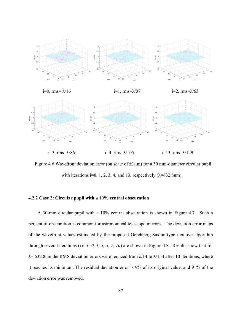
87

-100

1020

30

-100

10

2030-1

-0.5

0

0.5

1

mmmm

mic

ron

-100

1020

30

-100

10

2030-1

-0.5

0

0.5

1

mmmm

mic

ron

-100

1020

30

-100

10

2030-1

-0.5

0

0.5

1

mmmm

mic

ron

i=0, rms= λ/16 i=1, rms=λ/37 i=2, rms=λ/63

-100

1020

30

-100

10

2030-1

-0.5

0

0.5

1

mmmm

mic

ron

-100

1020

30

-100

10

2030-1

-0.5

0

0.5

1

mmmm

mic

ron

-100

1020

30

-100

10

2030-1

-0.5

0

0.5

1

mmmm

mic

ron

i=3, rms=λ/86 i=4, rms=λ/105 i=13, rms=λ/129


with iterations i=0, 1, 2, 3, 4, and 13, respectively (λ=632.8nm).

4.2.2 Case 2: Circular pupil with a 10% central obscuration

A 30-mm circular pupil with a 10% central obscuration is shown in Figure 4.7. Such a

percent of obscuration is common for astronomical telescope mirrors. The deviation error maps

of the wavefront values estimated by the proposed Gerchberg-Saxton-type iterative algorithm

through several iterations (i.e. i=0, 1, 3, 5, 7, 10) are shown in Figure 4.8. Results show that for

λ= 632.8nm the RMS deviation errors were reduced from λ/14 to λ/154 after 10 iterations, where

it reaches its minimum. The residual deviation error is 9% of its original value, and 91% of the

deviation error was removed.

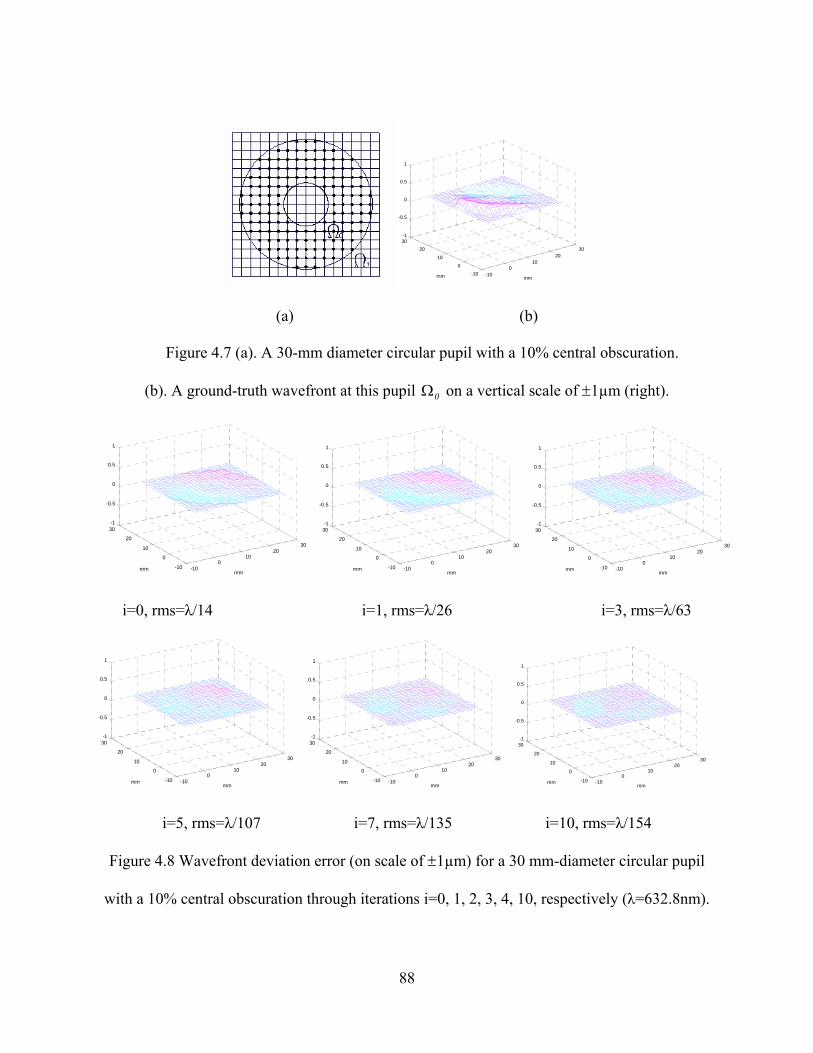
88

-100

1020

30

-100

10

2030-1

-0.5

0

0.5

1

mmmm

(a) (b)

Figure 4.7 (a). A 30-mm diameter circular pupil with a 10% central obscuration.

(b). A ground-truth wavefront at this pupil 0Ω on a vertical scale of ±1µm (right).

-100

1020

30

-10

0

10

20

30-1

-0.5

0

0.5

1

mmmm -10

010

2030

-10

0

10

20

30-1

-0.5

0

0.5

1

mmmm -10

010

2030

-10

0

10

20

30-1

-0.5

0

0.5

1

mmmm


-100

1020

30

-10

0

10

20

30-1

-0.5

0

0.5

1

mmmm -10

010

2030

-10

0

10

20

30-1

-0.5

0

0.5

1

mmmm -10

010

2030

-10

0

10

20

30-1

-0.5

0

0.5

1

mmmm



with a 10% central obscuration through iterations i=0, 1, 2, 3, 4, 10, respectively (λ=632.8nm).

89

4.2.3 Algorithm convergence

The deviation error reduction through Gerchberg-Saxton-type iterations was found to be

efficient. Specifically, the final deviation errors after a maximum of 4 iterations for the two

examples considered are less than λ/100 for λ equal to 632.8nm, as shown in Figures 4.6 and 4.8.

The convergence indicated by the RMS wavefront error in units of wavelength as a function of

the number of iterations is plotted in Figure 4.9. Such a finding is high performance for optical

testing, and the algorithm can be said to be very efficient.

0 5 100.00

0.02

0.04

0.06

0.08

0.10

Dev

iatio

n er

ror(

unit:

λ=6

32.8

nm)

Iterations

Data 1,No obstruction Data 2, Central obstruction

Figure 4.9 Plot of RMS deviation errors as a function of the number of iterations

90

4.3 Computational complexity

In the proposed iterative wavefront estimation algorithm, there are three linear matrix

equation sets that need to be solved at each iteration: One is the matrix equation set for

wavefront estimation from the slope data, and the other two are the matrix equation sets for y-

slope and z-slope computations from the estimated wavefront across iterations. The three matrix

equation sets are highly sparse. If we define a fill-in factor, an indicator of matrix sparseness, as

the quotient of the number of nonzero elements to the total number of the matrix elements, then

the fill-in factor of the wavefront estimation matrix CCT is 3)/t4t5( − , and the fill-in factors of

the slope computation matrices AAT and BBT are both 3)/t4(t + . For example, the fill-in factors

of the wavefront estimation matrix and the slope computation matrices are 4.6% and 1.4%

respectively for t=10, and they decrease to 0.05% and 0.01% at t=100. Besides their high

sparsity, all three matrices are symmetrical, positive and banded, once the wavefront “zero-

point” has been determined for the wavefront estimation.

4.3.1 Computational complexity of the proposed iterative algorithm

The computational complexity includes the spatial complexity and the time complexity.

The spatial complexity is a measure of memory needed for computation when the algorithm

runs, whereas the time complexity measures how much computation (thereby computation time)

is needed for the algorithm to converge to the solution.

91

4.3.1.1 Spatial complexity

The extremely regular and symmetrical banded matrices of the three linear equation sets

allow mapping the estimation matrix as a function of the index number of the matrix rows and

columns, because the nonzero elements in these matrices are regularly patterned with the

numbers 4,3,2,1,-1 only. Thus the problem of matrix storage is avoided in solving each equation

except for about 3t elements memory space reserved for the banded Cholesky decomposition

of CCT , which is a much smaller part in comparison with the 2/t 4 element space needed for a

conventional Cholesky decomposition. Naturally, a memory space of 2t3 elements is necessary

in each linear equation for storing the slope data and the wavefront values.

4.3.1.2 Time complexity (Impact on computation time)

Before we discuss the computational complexity of our algorithm, we shall introduce

“FLOPS”, an abbreviation of “Floating-Point Operations”, to denote the arithmetic operations

that a computer performs, such as multiplications, additions (or subtractions).182

The positive definite slope-extraction matrices AAT and BBT are banded diagonal matrices

with their semi-bandwidths of 2 and t, respectively. In computing the slope data from a given

wavefront, it is an advantage to employ a direct solution method, such as the Cholesky method,

because we can decompose the matrices AAT or BBT into two unique triangular matrices once

and for all by several steps of derivation. Therefore no more Cholesky decompositions are

needed in computation. The computations needed in solving the two systems of equations are

substitutions, and the corresponding arithmetic cost is approximately a product of m4 with the

92

bandwidth,182 which yields 28t FLOPS for AAT and 3t4 FLOPS for BBT . As a comparison,

the computational cost needed for substitutions in solving an equation without exploiting the

band structure is 4t2 FLOPS. 182

To solve the matrix equation set for wavefront estimation, we need to set a “zero-point” for

the wavefront under estimation to make the matrix CCT positive and definite so that we can

make Cholesky decomposition with CCT , which is a banded sparse matrix with a bandwidth of

t2 . An algorithm for solving the wavefront estimation equations based on the banded Cholesky

decomposition needs about 34 t4t + FLOPS in total, where 4t FLOPS is used for decomposition

and 3t4 FLOPS for substitutions.182 As a comparison, a solving algorithm based on the

conventional Cholesky decomposition without exploiting the band structure of the matrix yields

about 6t31 FLOPS for decomposition and 4t2 FLOPS for substitutions.

Other direct solution methods are also available in solving the above three equation sets,

such as Gaussian Elimination and SVD methods, but such methods are more computationally

intensive. Generally, the conventional Gaussian Elimination method has a cost of about 6t32

FLOPS, and the SVD method needs about 6t12 FLOPS.183 Because the SVD method yields a

unique LSMN for a rank deficient least-squares problem, it is a good method in practice if the

computational complexity is not a constraint.

An alternative to solving the matrix equation set is to use iterative methods, such as the SOR

method, which is said to be one of the most efficient among the classical iterative methods. The

convergence rate of the SOR method is closely related to the problem model, the discretization

mesh size, the relaxation factor, and the grid indexing orders. However, the iterations needed for

93

the optimal SOR method to converge to a solution within a precision of 810− can be estimated

by 181, 182

t3)1(t94.2))1tπ21(log(8R 1

10ωb ≈+≈−

−−= − . (4.37)

So if it requires approximately 2t5 FLOPS operations in iteration,181 the computational cost

needed for solving Eq. (4.7) with the optimal SOR method is about 3t15 FLOPS.

Comparing with the banded Cholesky decomposition method, which needs 34 t4t + FLOPS

of cost for solving Eq. (4.7), the SOR method is computationally more intensive for a small grid

size (t<11), and less intensive for a large grid size (t>11). The complexity of the optimal SOR

method increases as a cubic curve, whereas the complexity of the banded Cholesky method

increases with a quartic curve.

4.3.2 Complexity comparison with the FFT-based iterative algorithms

4.3.2.1 Comparison of time complexity

The fast Fourier transform (FFT) of a data set of length q2m = (q is a positive integer)

requires about (m)logm 2 complex multiplications, which is equivalent to (m)logm5 2 FLOPS of

arithmetic operations according to a detailed analysis (Brigham 1988).184, 185 The FFT-based

iterative algorithm proposed by Roddier and Roddier(1991) needs to compute two FFTs besides

the computations of the y- and the z-slopes from the wavefront at each iteration.92 Therefore, if

we suppose that the computation of the slope extractions takes the same computational cost in

94

both algorithms and we ignore this cost, the computational cost needed in one iteration of the

FFT-based iterative algorithm is about 22 )t7)t(log20( + FLOPS, which is usually much smaller

than that of the optimal SOR-based (i.e. 3t15 FLOPS) iterative algorithm. Thus, based on the

computational complexity evaluation of one iteration, the FFT-based algorithm is superior in

performance to the proposed algorithm, which could be significant for large values of grid-array

size t (t× t=m).

At the same time, the required number of iterations for each algorithm will significantly

affect the overall computational time. The number of iterations is a factor of the overall grid-

array size and measurement noise levels, etc. The FFT-based algorithms usually converge

slowly; for example, the Gerchberg-Saxton algorithm needs at least tens to hundreds or even

thousands of iterations to converge to a solution, while we found that the algorithm proposed in

this paper converges to less than λ/100 deviation error with only four iterations.

4.3.2.2 Comparison of spatial complexity

It has been established that the space complexity required for a Fast Fourier Transform

(FFT) is ( )4tO , which is used for the storage of complex matrix arrays. As a comparison, the

spatial complexity for the Gerchberg-Saxton-type iterative algorithm we have proposed with the

banded Cholesky solution method is only ( )3tO .

Some relatively subtle difference between the Roddier & Roddier (1991) algorithm and

the algorithm proposed here is the fact that in performing FFTs, the square array matrix satisfies

m=2q, and therefore m must be even. In the case of the proposed algorithm, there is no such

95

requirement, and we have shown that odd matrix sizes yield lower error propagation than even

matrix sizes.

4.4 Error propagation estimation

If we ignore the perturbations introduced by the computer rounding errors, wavefront errors

may occur from two sources: the algorithm discretization errors, which depend on the basic

estimation scheme adopted, and the wavefront sensor measurement error such as the CCD

centroiding error. The discretization errors of the wavefront estimation scheme adopted were

discussed in a previous literature.11 In this section, we qualitatively study the propagation of the

wavefront measurement error in wavefront estimation by evaluating the condition number of the

wavefront estimation matrix. The quantitative analysis of the error propagation in wavefront

estimation will be detailed in Chapter 5.

The condition number of a wavefront estimation matrix is an amplification factor for the

error propagation in wavefront estimation. Regarding the pre-defined wavefront estimation

matrix equation in Eq. (4.7), the condition number of CCT can be defined as

( )[ ]1T2

T2

T lub)(lub:)cond( −= CCCCCC , (4.38)

where )(lub2 ⋅ is a matrix norm defined (for example, for matrix C) by

[ ] 2/1T2/1

T

TT

0X2 )(max)(lub CCXXCXCXC ρ=⎟⎟

⎠

⎞⎜⎜⎝

⎛=

≠, (4.39)

which is a corresponding matrix norm of the Euclidian norm of a vector X ( ) 2/1T XXX2= .

Then we have

96

[ ]1TTT )()()cond( −ρρ= CCCCCC , (4.40)

where )( T CCρ is the spectral radius of CCT . Since maxT )( λ=ρ CC , then [ ] 1

min1T )( −− λ=ρ CC ,

where maxλ and minλ are the maximum and minimum eigenvalues of the matrix CCT ,

respectively. Therefore the condition number of CCT can be written as

min

maxT )cond(λλ

=CC . (4.41)

If matrix CCT is invertible, the wavefront estimation error ( )Tm21 ΔwΔwΔwΔ L=W can

be estimated by

( ) WFDT1T ΔΔ SCCCW −

= , (4.42)

where WFDΔS is the WFD measurement error vector. Applying Euclidian norm on both sides of

Eq. (4.42) yields 181, 11, 186

[ ]( ) 2WFD

2

21

T

2Δ

lub)cond(Δ S

CCCW ≤ . (4.43)

In Chapter 5, we will show that SCS Δa21Δ sWFD = for the Southwell geometry, where a is

the pitch size of the sampling grid array, ( )Tm21 ΔsΔsΔsΔ L=S is the wavefront slope

error vector, and sC is a matrix used to convert a slope vector to a WFD vector. Therefore

[ ] ( )( ) 2

21

min

msxS2

21

2

s221

T2

Δa21Δ

lublub)cond(a

21Δ SS

CCCCW

λλ

=⎥⎦

⎤⎢⎣

⎡≤ , (4.44)

where maxSλ is the maximum eigenvalue of matrix sT

s CC .

If the wavefront slope errors are independent and have the same variance 2sσ , then

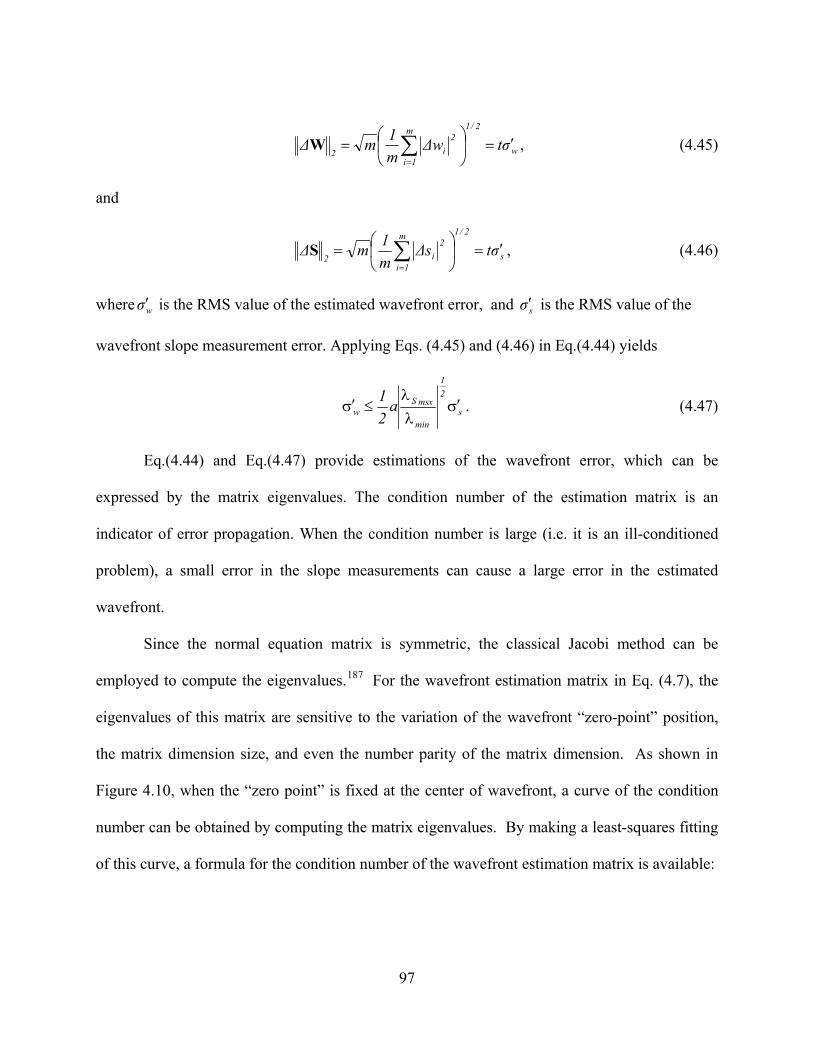
97

w

2/1m

1i

2i2

σtwΔm1mΔ ′=⎟

⎠

⎞⎜⎝

⎛= ∑

=

W , (4.45)

and

s

2/1m

1i

2i2

σtsΔm1mΔ ′=⎟

⎠

⎞⎜⎝

⎛= ∑

=

S , (4.46)

where wσ′ is the RMS value of the estimated wavefront error, and sσ′ is the RMS value of the

wavefront slope measurement error. Applying Eqs. (4.45) and (4.46) in Eq.(4.44) yields

s

21

min

msxSw a

21

σ′λλ

≤σ′ . (4.47)

Eq.(4.44) and Eq.(4.47) provide estimations of the wavefront error, which can be

expressed by the matrix eigenvalues. The condition number of the estimation matrix is an

indicator of error propagation. When the condition number is large (i.e. it is an ill-conditioned

problem), a small error in the slope measurements can cause a large error in the estimated

wavefront.

Since the normal equation matrix is symmetric, the classical Jacobi method can be

employed to compute the eigenvalues.187 For the wavefront estimation matrix in Eq. (4.7), the

eigenvalues of this matrix are sensitive to the variation of the wavefront “zero-point” position,

the matrix dimension size, and even the number parity of the matrix dimension. As shown in

Figure 4.10, when the “zero point” is fixed at the center of wavefront, a curve of the condition

number can be obtained by computing the matrix eigenvalues. By making a least-squares fitting

of this curve, a formula for the condition number of the wavefront estimation matrix is available:

98

⎪⎩

⎪⎨⎧

+−

+−=even is t .e75.22316.355

odd is t, e87.15044.243)cond(83.6t

52.7t

T CC , (4.48)

where t is the matrix dimension number (t×t=m) . Results show that the wavefront estimation

has a better performance in error propagation when the dimension number of the estimation

matrix is odd. Therefore, an odd-number sampling grid array is preferable in wavefront

estimation. When the matrix dimension becomes larger, the Jacobi method converges slowly. It

takes about 68000 iterations to obtain the eigenvalues with 10-7 accuracy for the case of t=15.

4 6 8 10 12 14 16

0

500

1000

1500

Con

ditio

n N

umbe

r

Grid size(t)

% (Even number of Grid size) % (Odd number of Grid size)

Figure 4.10 The condition number of normal estimation matrix versus grid dimension size.

The above analysis is also applicable to the error propagation of slope computation

provided by Eqs. (4.22) and (4.36). The eigenvalues of the two slope-computation matrices in

99

Eqs.(4.22) and (4.36) are found to be 22 − , 22+ and 4 when t> 4, and the eigenvalues are

22 − and 22+ only for t =4. Thus the condition numbers of these two matrices are

both 836224 .)/( ≈− for t>4, and 8352222 .)/()( ≈−+ for t=4. Therefore, such condition

numbers indicate that the error propagation in the y- (or equivalently z-) slope computation is

very stable and very slow.

4.5 Summary

Klaus Freischlad in 1992 pointed out that a wavefront estimation algorithm that is suitable

for practical optical testing must have the following characteristics:120 (1) The wavefront

estimates must be unbiased; (2) The error propagation coefficient must be slow; (3) The

computation must be efficient, especially for large datasets; (4) The necessary memory space

should be small enough to be applicable in the laboratory; Finally, (5) the algorithm should be

easily adaptable to various pupil shapes. In this chapter with the domain extension technique, a

pre-defined wavefront estimation matrix and the associated pre-defined slope-computation

matrices for any pupil shape or size were obtained. A Gerchberg-Saxton-type iterative process

based on the linear least-squares estimation has been implemented to obtain a practical unbiased

wavefront estimation algorithm for any pupil shape, which combines the accuracy of the

Gerchberg-Saxton-type iterative wavefront slope extrapolation technique with the efficiency of

linear sparse matrix.

In summary, the proposed iterative algorithm has the following features: (1) To our

knowledge it is the first time that the Gerchberg-Saxton iterations were implemented by linear

100

least-squares matrix estimations. (2) It does not have the 2π-phase ambiguity problem that all

FT-based Gerchberg-Saxton algorithms suffer from, so it is good for phase retrieval with large

aberrations. (3) It provides a once-for-all pre-defined wavefront estimation matrix that is good

for any pupil size without apriori knowledge of the pupil shape. (4) It is a fast-converging

iterative algorithm, which was demonstrated with some examples, that converges much faster

than the FT-based Gerchberg Saxton algorithm. (5) It has high estimation accuracy. The

deviation error can be less than λ/150 as shown in the examples. (6) Its error propagation is slow

in wavefront estimation. An analysis of error propagation showed that the wavefront estimation

matrix is well-conditioned, yielding low propagation errors.

A U.S. patent has been filed in the United States of America regarding this iterative

wavefront estimation algorithm.188

101

CHAPTER FIVE: QUANTIFICATIONS OF ERROR PROPAGATION IN WAVEFRONT ESTIMATION

5.1 Introduction

As discussed in Chapter 3, the wavefront estimation is a numerical solution to the

Neumann’s boundary problem of Poisson equation. Using a 2-D finite difference grid to cover

the testing domain, one can discretize this problem, and evaluate the wavefront values at each

grid point by solving a difference equation set defined on the grid. The matrix equation set for

this problem, as shown in Eq. (4. 5b), can be expressed as

SCW = , (5. 1)

where C is the wavefront estimation matrix, W is the vector of wavefront values, and S is the

vector of the WFD between the neighboring grid points, which can be converted from the

wavefront slope vector G by

MGS aμ= , (5. 2)

where μ is a constant related to the given geometry, a is the pitch size of the sampling grid,

and M is the conversion matrix for a given geometry.

Owing to the measurement noise, Eq.(5.1) has weak solutions only, and an unbiased

least-squares approximation can be employed. The normal matrix equation for the least-squares

solution is

SCCWC TT = , (5. 3)

102

which is a discretization form of the Poisson equation as shown in Eq. (3.8). It shall be noted that

the Tikhonov regularized least-squares solution, adopted widely in other applications such as

adaptive optics, provides a biased estimate that would not be desirable in optical testing. 189

The noisy WFD vector can be written as NSS += 0 , where 0S is the vector of the true

WFD values, and N is the measurement noise of the WFD. If the induced wavefront error from

measurement noise N is ε , then the estimated wavefront can be written as εWW += 0 , where

0W is the true wavefront values. The error propagation coefficient provides a quantitative metric

for evaluating wavefront estimation. As defined in the previous literature,87,88,120 the error

propagation coefficient η is the ratio of the mean variance of the wavefront estimation error

2wσ given by

/mσ 2

22w ε= , (5. 4)

where2⋅ is the Euclidian norm and m is the total number of grid points ( ttm ×= for a square

array, t is the grid size), to the mean variance of the WFD measurement error 2nσ

, i.e.

2n

2w

σση = . (5. 5)

This definition is referred to as the WFD-based error propagation coefficient, which is a

quantitative indicator of the error propagator in the WFD-based wavefront estimation. In this

chapter, we present a general formulation for the WFD-based error propagation coefficient with

the matrix eigenvalue method (Zou and Rolland, 2004, 2006).190,191 With the serial numbering

wavefront estimation scheme introduced, the general error propagation formulation is

implemented for the Hudgin geometry, the Southwell geometry and the Fried geometry.190

Based on the WFD-based error propagation coefficient formulation, the definition of the slope-

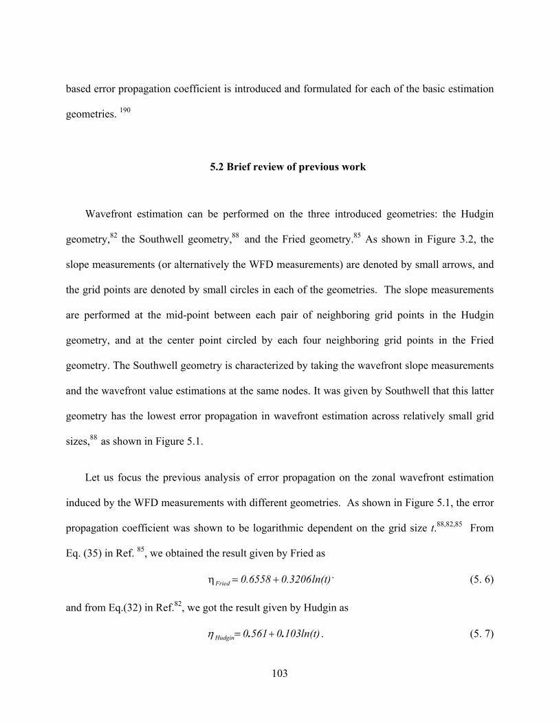
103

based error propagation coefficient is introduced and formulated for each of the basic estimation

geometries. 190

5.2 Brief review of previous work

Wavefront estimation can be performed on the three introduced geometries: the Hudgin

geometry,82 the Southwell geometry,88 and the Fried geometry.85 As shown in Figure 3.2, the

slope measurements (or alternatively the WFD measurements) are denoted by small arrows, and

the grid points are denoted by small circles in each of the geometries. The slope measurements

are performed at the mid-point between each pair of neighboring grid points in the Hudgin

geometry, and at the center point circled by each four neighboring grid points in the Fried

geometry. The Southwell geometry is characterized by taking the wavefront slope measurements

and the wavefront value estimations at the same nodes. It was given by Southwell that this latter

geometry has the lowest error propagation in wavefront estimation across relatively small grid

sizes,88 as shown in Figure 5.1.

Let us focus the previous analysis of error propagation on the zonal wavefront estimation

induced by the WFD measurements with different geometries. As shown in Figure 5.1, the error

propagation coefficient was shown to be logarithmic dependent on the grid size t.88,82,85 From

Eq. (35) in Ref. 85, we obtained the result given by Fried as

ln(t)3206.06558.0Fried +=η , (5. 6)

and from Eq.(32) in Ref.82, we got the result given by Hudgin as

ln(t)10305610Hudgin .. +=η . (5. 7)

104

For the Southwell geometry, we least-squares fit our discrete coordinate measurements of curve

A in Fig.2 on page1003 of Ref.88 given by Southwell, and obtained

ln(t)29630104470Southwell .. +−=η . (5. 8)

By using a general Green’s function and neglecting the boundary conditions, Noll

analytically derived that the error propagation is a logarithmic dependent function of its grid size

t. For a square aperture with the phase value at the origin set to be zero, the coefficient was can

be obtained by 87

ln(t)318010720Noll .. +=η . (5. 9)

Figure 5.1 Previous results on error propagation

105

In modal estimation with discrete Fourier transform, Freischlad and Koliopoulos also

showed that the error propagation satisfies a logarithmic dependence of ln(t)π1aη modal S;H, += for

the Hudgin geometry and the Southwell geometry, and a logarithmic dependence of

1)-ln(tπ3aη modF; += for the Fried geometry. 119 On the basis of the Hudgin geometry and a fast

FT-based algorithm, which requires an even size, Freischlad confirmed that it is almost identical

to Noll’s theoretical result with 120

ln(t)1097530Freischlad πη += . . (5. 10)

Hunt extended Hudgin’s method for error coefficient prediction in terms of the discrete

Fourier transform and obtained a result that shares the constant term with Noll and the

logarithmic term with Fried and Hudgin, which yields little difference from both Noll’s and

Freischlad’s results.86

Figure 5.1 shows that the Southwell geometry is superior to all the other geometries

regarding the error propagation when t is small, but the Hudgin geometry tends to be slightly

superior to the Southwell geometry when the grid array size t becomes large (when t>30).

5.3 Formulation of the error propagation with matrix method

Given Eq.(5.1) and considering that in the case of zero noise Eq.(5.1) reduces to 00 CWS = ,

the WFD error N and the induced wavefront error ε should satisfy the equation

NCε = . (5. 11)

In a general case, the least-squares solution for Eq. (5.11) can be written as

106

NCε += , (5. 12)

where +C is the Moore-Penrose pseudo-inverse of matrixC . Given the relationship between the

WFD vector and the wavefront slope vector provided by Eq. (5.2), similarly the WFD error N

and the wavefront slope noise N′ should satisfy

NMN ′= aμ . (5. 13)

Starting with the expression of the mean variance given by Eq. (5.4), the Euclidian norm

for a statistical wavefront error vector is defined as

( )21

T21

m

1j

2j2

tr εεε =⎟⎟⎠

⎞⎜⎜⎝

⎛ε≡ ∑

=

, (5. 14)

where the bracket ⋅ denotes the averaging operator, ( )⋅tr is the matrix trace. And

( ) ( )TTTTTT aa ++++ μ′′μ== CMNNMCCNNCεε , (5. 15)

where TNN ′′ is given by 189

⎥⎥⎥⎥⎥

⎦

⎤

⎢⎢⎢⎢⎢

⎣

⎡

=′′

2m2m1m

m22212

m12121

T

nnnnn

nnnnnnnnnn

L

MOMM

L

L

NN . (5. 16)

If we simply assume that the wavefront slope noise is random, independent, and has zero

mean with the same variance 2sσ , the ensemble statistical average of the slope errors yields

⎩⎨⎧

=≠

==ji when,σji when ,0

δσnn 2s

ij2sji . (5. 17)

So the slope noise covariance matrix is given by

107

INN 2s

T σ=′′ , (5. 18)

where I is the identity matrix. Therefore, Eq.(5.15) yields

( )TT2s

22T a ++σμ= CMMCεε . (5. 19)

Accordingly the mean variance of the wavefront estimation error 2wσ is given by,

( )[ ]TT2s

22T2

22w tr

matr

m1

m1σ ++=== CMMCεεε σμ . (5. 20)

Similarly, the variance of the WFD measurement error 2nσ is given by

T2s

22T2

22n tr

matr

m1

m1σ MMNNN σμ

=== . (5. 21)

With the definition of the error propagation coefficient given in Eq. (5.5), we can write

( )[ ][ ]T

T

2n

2w

trtr

σση

MMMCMC ++

== . (5. 22a)

This equation is useful for the computation of the error propagation coefficient. It can be noted

that Eq.(5.22a) can also be written in the form of the Frobenius norm187 as

2

F

2

FηM

MC+

= . (5.22b)

Equations (5.22) provide a generalized expression for the error propagation coefficient in

zonal wavefront estimation. This formula is good for either the slope measurements or the direct

WFD measurements, because we can convert either the slope measurements or any other specific

WFD measurements into the wavefront value difference between each pair of the neighboring

grid points, which is actually the direct WFD measurement in the Hudgin geometry.

108

Figure 5.2 Grid array with serial numbering scheme

In next Section, the serial number scheme (SNS) will be adopted for wavefront

estimation in studying the error propagation for each of the basic geometries. The SNS, as

adopted in Chapter 4 and the previous literatures189,11, makes wavefront estimation become a

standardized process. Instead of numbering the estimation grid array with 2-D coordinates ( )ji,

as previously provided, 82,85,88,120 the grid array is indexed sequentially from 1 to m row by row as

illustrated in Figure 5.2 for a square domain. With such a numbering mode, a regular and

banded sparse estimation matrix is pre-defined, which resembles Hunt’s matrix formulation.11, 86

5.4 Quantification of Wavefront difference-based error propagation

In this section, the WFD-based error propagators for Hudgin, Southwell and Fried

geometries are formulated and their behaviors compared. As alternative to the WFD-based

definition, the wavefront slope-based error propagators are also defined, and the formulations for

different geometries are derived.

109

5.4.1 Wavefront difference-based error propagators

For the WFD-based wavefront estimation, we apply the general formula of the error

propagation coefficient we developed for the three basic estimation geometries: the Hudgin

geometry, the Southwell geometry and the Fried geometry. With SNS the wavefront estimation

matrix for each of the geometries is established, and the eigenvalues for each of the estimation-

related matrix are numerically computed, from which the formulas of the WFD-based error

propagation coefficients are obtained.

5.4.1.1 Hudgin Geometry

In the Hudgin geometry, the wavefront slopes are measured at the mid-point

between two neighboring grid points, and the WFD between each pair of neighboring grid

points in the x-and y-directions can be estimated as

⎩⎨⎧

==

++

++

agsags

ti,iti,i

,i1i,i1i

yy

xx , (5. 23)

where a is the pitch size of the sampling grid array, ,i1ixg

+is the wavefront slope in the x-

direction at the midpoint between point i and point 1i + , and tiiyg

+,is the wavefront slope in

the y-direction at the midpoint between point ti + and point i . With the SNS mode the

wavefront estimation equations can be written in the x-direction as

integerkt, k ,...,m, i2,1, isww,i1ixi1i ≠==−

++ , (5. 24)

and in the y-direction as

t-2,..m 1,i ,swwtii,ytii ==−

++ . (5. 25)

110

When written in matrix form, the estimation equation set for the Hudgin geometry is

given by

SHW = , (5. 26)

where H is the wavefront estimation matrix, S=aG is the WFD vector, and G is the wavefront

slope vector. In comparison with Eq. (5.2), S=aG yields 1=μ and IM = , where I is the identity

matrix. According to Eqs. (5.22a) and (5.22b), where C equals H for the Hudgin geometry,

η takes the form

( )[ ][ ] ( )[ ] 2

F

TT

m1tr

m1

trtrη ++

++

=== HHHIHH

H . (5. 27)

In optical testing, it is the wavefront shape from a reference, not the absolute wavefront

piston values, that is desirable. Thus it is common to set a point on the wavefront as the reference

point, namely the “zero point”, at which the wavefront value is assigned to zero or other

constant. Setting a “zero point” for the wavefront will not affect the estimated shape, as any

piston value in the estimation can be subtracted.

The rank of matrix HHT is 1−=γ m .11 Matrix HHT will become of full rank ( m=γ )

if a “zero point” is set for the wavefront. If HHT is of full rank in column, then its generalized

inverse matrix is TT HH)(HH 1−+ = , and ( )[ ] [ ]1TTtrtr −++ = H)(HHH . If the nonzero eigenvalues

of matrix ( )HHT are 0λ i >,H ( )1,2,..γi = , then the nonzero eigenvalues of matrix ( )+HHT are

0λ 1i >

−,H ( )1,2,..γi = . The WFD-based error coefficient for the Hudgin geometry can be therefore

expressed as

( )[ ] ⎟⎟⎠

⎞⎜⎜⎝

⎛==η ∑

γ

=

−+

1i

1i,

T λm1tr

m1

HH HH . (5. 28)

111

This result is somewhat similar to the result obtained by Southwell for modal wavefront

estimation. Southwell formulated the error propagation in the modal estimation, showing that the

mean-square phase error is proportional to the trace of ( ) 1−+AA .88

The numerical methods, such as the Jacobi and the SVD methods, can be employed to

evaluate the matrix eigenvalues. The Jacobi method approximates the eigenvalues of

symmetric matrices by reducing the off-diagonal elements to zero, while the SVD method

approaches the eigenvalues by decomposing the matrix into a diagonal matrix multiplied by an

orthonormal matrix on each side.

The eigenvalues of matrix HHT are sensitive with the position of the wavefront “zero

point”, the matrix dimension size, and the number parity of the matrix dimension. In this

problem, the “zero point” mentioned is located at the center point of the estimation grid array

for all geometries, at which the matrix has its smallest condition number.11 Given that the

coefficients in matrix HHT are pre-defined, the eigenvalues of matrix HHT for different grid

sizes can be computed numerically. The simulation results are plotted in Figure 5.3.

Fitting the numerical results (up to t=50) in the least-squares sense, we obtain the error

propagation coefficients for the Hudgin geometry as

(t)ln0.33160.32220.6672)-(tln3171.03797.0odd,H +≈+=η , odd) is t ( (5. 29)

and

(t)ln0.48560.30490.2136)-(tln4795.03294.0even,H +≈+=η . even) is (t (5. 30)

When no “zero point” is appointed, the rank of the matrix HHT is 1mγ −= . The solution

space for the matrix equation has one degree of freedom. With the Moore-Penrose pseudo-

inverse of the matrix HHT , we obtained the LSMN solution, which is a least-squares solution

112

that holds the same wavefront shape as that with a set “zero point” but has the minimum

Euclidian norm of the wavefront values. In that case, we computed the eigenvalues of the

estimation matrix with SVD, and obtained the simulation results with data up to t=50 as

(t)ln0.17640.26051.1208)-(tln1593.03252.0LSMN,H +≈+=η . (5. 31)

Figure 5.3 WFD-based error propagators for the Hudgin geometry

Figure 5.3 confirms that the behavior of the error propagation is logarithmic dependent

on the grid size as previously established in the literature.82,87 The error propagation curves for

the SNS with the “zero point” given (curves 2 and 3) are higher than the curves of Noll’s result

(Curve 0) and the Hudgin results (Curve 1). However, the error propagation curve for the SNS

113

with the LSMN solution (Curve 4) is the lowest of all, nevertheless, at the expense of extensive

computations; moreover, it is approaching the Hudgin result when the grid size increases. For

wavefront estimation with a “zero point” set, an odd-number grid size is preferable for the

Hudgin geometry.

5.4.1.2 Southwell Geometry

In the Southwell geometry the slope measurements and the wavefront estimate are

located at each grid point. As Southwell did,88 the average of the measured slopes over two

neighboring grid points is adopted as an estimate of the slope at the mid-point. The wavefront

estimation equation set can be obtained with the SNS in the x-and y-directions as

), g(g2aww

1ii xxi1i ++=−+ (5. 32)

where i=1,2,…,m-1( with kti ≠ , k is an integer), and ixg is the slope data in the x-direction, and

), g(g2aww

tii yytii ++=− + (5. 33)

where t-2,..m 1,i = , and iyg is the slope data in the y-direction. In matrix form,

HSHW = , (5. 34)

where matrix H is the same wavefront estimation matrix as for the Hudgin geometry, and HS is

the WFD vector , which is given by GCS sH a21

= . Comparing HS with Eq.(5.2), we

obtain 21 /=μ and sCM = . It should be noted that matrices sC and H are closely related:

matrix sC can be obtained by changing the sign of the coefficient “-1” in matrix H .

114

According to Eq. (5.22), we have

( )[ ][ ]

( )[ ][ ]T

sTT

sTss

Tss

S trtr

trtr

ηHH

CHHCCC

CHCH ++++

== , (5. 35)

where [ ] ( ) ( )tm41tt4tr T −=−=HH . Given ( ) TT HHHH++ = ,192 then the WFD-based error

propagation coefficient for the Southwell geometry is expressed as

( )[ ]( )

( )[ ]( )tm4

tr

tm4tr

ηs

2Ts

sTT

sS −

⎥⎦⎤

⎢⎣⎡

=−

=

+++ CHHHHCCHHC

TT

. (5. 36)

Finally,

( ) ⎟⎟⎠

⎞⎜⎜⎝

⎛=η ∑

γ

=1iis,S λ

t-m41 , (5. 37)

where i s,λ (i=1,2,… γ ) are the nonzero eigenvalues of matrix ( )[ ] sT

2TT

s CHHHHC + , and γ is

the rank of this matrix.

When a “zero point” is set, HHT is invertible, and we have m=γ and ( ) T1T HHHH−+ = .

The simulation results are shown in Figure 5.4. We least-squares fit the numerical results (up to

t=50), and obtain the error propagation coefficients for the Southwell geometry as

(t)ln0.29521428.00.06186)-(tln2936.01489.0odd,S +≈+=η , ) odd is (t (5. 38)

and

)t(ln0.410.2861)7673.2(tln4662.004941.0even,S +≈++=η . even) is t ( (5. 39)

When no “zero point” is appointed, the LSMN solution is sought to make the Euclidian

norm of the wavefront minimum. We computed the eigenvalues of the estimation matrix for this

case by SVD up to t=50, and obtained the error propagation coefficient as

(t)ln0.14550.2170.2562)(tln1487.0205.0LSMN, +≈++=ηS (5. 40)

115

Figure 5.4 WFD-based error propagators for the Southwell geometry

In Figure 5.4, when a wavefront “zero point” is assigned, the error propagation curve for

the SNS is above the curve of Noll’s result (Curve 0) for the even-number grid sizes (Curve 3),

and it is equivalent to (or slightly below) it for the odd-number grid sizes (Curve 2). Although

both of the above mentioned two error propagators (Curve2 and Curve 3) are shown to be worse

than the Southwell’s result (Curve 1), the error propagator of the LSMN solution (Curve 4),

when no “zero point” is set for the wavefront, is showed to be clearly better for the large grid

size(t>8). Similar to the Hudgin geometry, an odd-number grid size is preferable for the

Southwell geometry when a “zero point” is assigned.

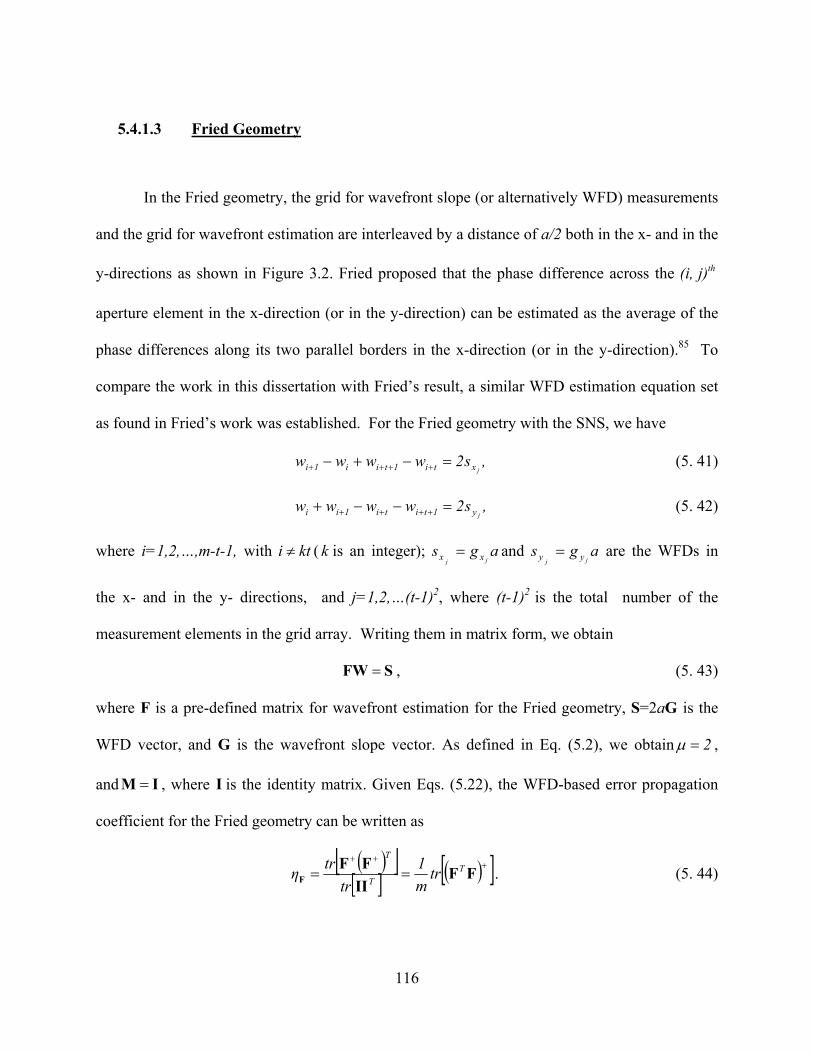
116

5.4.1.3 Fried Geometry

In the Fried geometry, the grid for wavefront slope (or alternatively WFD) measurements

and the grid for wavefront estimation are interleaved by a distance of a/2 both in the x- and in the

y-directions as shown in Figure 3.2. Fried proposed that the phase difference across the thj) (i,

aperture element in the x-direction (or in the y-direction) can be estimated as the average of the

phase differences along its two parallel borders in the x-direction (or in the y-direction).85 To

compare the work in this dissertation with Fried’s result, a similar WFD estimation equation set

as found in Fried’s work was established. For the Fried geometry with the SNS, we have

, s2wwwwjxti1tii1i =−+− ++++ (5. 41)

, s2wwwwjy1titi1ii =−−+ ++++ (5. 42)

where i=1,2,…,m-t-1, with kti ≠ ( k is an integer); agsjj xx = and ags

jj yy = are the WFDs in

the x- and in the y- directions, and j=1,2,…(t-1)2, where (t-1)2 is the total number of the

measurement elements in the grid array. Writing them in matrix form, we obtain

SFW = , (5. 43)

where F is a pre-defined matrix for wavefront estimation for the Fried geometry, S=2aG is the

WFD vector, and G is the wavefront slope vector. As defined in Eq. (5.2), we obtain 2=μ ,

and IM = , where I is the identity matrix. Given Eqs. (5.22), the WFD-based error propagation

coefficient for the Fried geometry can be written as

( )[ ][ ] ( )[ ]+++

== FFIIFF

FT

T

T

trm1

trtrη . (5. 44)

117

Herrmann showed that the rank of the normal matrix FFT is m-2.91 If the nonzero

eigenvalues of FFT are 0i ,F >λ (i=1, 2, … γ ), where γ is the rank of matrix FFT ,then

⎟⎟⎠

⎞⎜⎜⎝

⎛=η ∑

γ

=

−

1i

1iF λ

m1

F, . (5. 45)

When a grid point is frozen as the “zero point”, the rank of matrix FFT

becomes 1m −=γ , and the piston value term of the estimated wavefront is defined. However,

there is still one degree of freedom in the least-squares solution space, called the “waffle mode”,

at which the wavefront at the estimation grid points can be pushed up and down with the same

value in a checkerboard pattern, while it still satisfies the WFD estimation equation set defined in

Eqs.(5.41) and (5.42). In other words, the Fried geometry can not sense the waffle mode error of

the wavefront,193 which is not desirable in optical testing.

Given a “zero point” for the wavefront, the LSMN solution is to seek a least-squares

solution in a one dimensional (1-D) solution space that makes the Euclidian norm of the

wavefront shape minimum. While no “zero point” is assigned for the wavefront, we have

2m −=γ , and the LSMN solution is to seek a least-squares solution in a two-dimensional

solution space (LSMN (2-D)) to minimize the Euclidian norm of the wavefront shape, which

includes both the overall piston mode and the waffle mode errors. Theoretically, when the

wavefront shape is flat, the LMSN solution can get rid of the waffle mode error. However, since

the waffle mode error usually coexists with the wavefront shape, it is impossible to avoid the

waffle mode error for the Fried geometry with the LMSN solution. The simulation results are

shown in Figure 5.5.

118

Figure 5.5 WFD-based error propagators for the Fried geometry

For a wavefront with a “zero point” set, the matrix eigenvalues for the LSMN (1-D)

solution are computed up to t=50, which yields the error propagation coefficients as

(t)ln207.04146.0)8805.0(t-ln2.04461.0ηF,odd +=+= , ) odd is t ( (5. 46)

and

(t)ln3022.04338.0)6547.0(t-ln2866.04933.0ηF,even +=+= . even) ist ( (5. 47)

For wavefront with no “zero point” set, the matrix eigenvalues for the LSMN (2-D) solution are

computed up to t=50, which yields the error propagation coefficients as

(t)ln1303.04076.0)821.1(t-ln114.0475.0ηF,LSMN +≈+= . (5. 48)

119

Similar to the Hudgin and Southwell geometries, for a wavefront with a “zero point” set, an odd-

number grid size is preferable for wavefront estimation. The LSMN(1-D) solution (Curves 2 and

3) offers error propagators better than Fried’s result(Curve 1); but the error propagator for the

even-number grid sizes (Curve 3) is worse than Noll’s result (Curve 0), whereas the one for the

large odd-number grid sizes(t>16) (Curve 2) is better than it. For a wavefront with no “zero

point” set, the LSMN (2-D) solution offers the best error propagator for the Fried geometry.

It should be noticed that for wavefront estimation with the Fried geometry, it can either

yield a LSMN solution on the full size of the estimation grid that suffers the waffle mode error,

or yield a least-squares solution on a subsized estimation grid by discarding some of the

wavefront boundary values (for example, the corner points). However, these solutions may not

be acceptable in some optical testing cases.

5.4.2 Comparisons of the error propagators

To compare the error propagations in different wavefront estimation schemes, the

simulation results for the Hudgin, Southwell and Fried geometries are plotted in Figure. 5.6. The

simulation results quantify how the error propagator depends on the parity of the wavefront

estimation grid size, the wavefront estimation scheme, and the solution method used for solving

the wavefront estimation.

Importantly, the odd-number grid sizes are shown to yield lower error propagation than

the even-number grid sizes for all geometries. This can be explained by the following: If the grid

size is odd, the “zero point” can be easily set at the geometrical center of the grid array so that

the estimation scheme is symmetric and yields an estimation matrix with its minimum condition

120

number,11 which is steady and less sensitive to random noise disturbance. However, if the grid

size is even, there is no direct way to set a “zero point” at the geometrical center of the sampling

grid; therefore, the estimation scheme is typically non-symmetric, which is liable to be affected

by random noise disturbance.

Figure 5.6 Comparison of the WDF-based error propagators

For wavefront estimation with a “zero point” set, the Fried geometry offers the best error

propagator for the even-number grid sizes, and the Hudgin geometry offers the worst for both

even- and odd-number grid sizes. For the odd-number grid size, the Southwell (t<22) and Fried

121

(t>22) geometries offer the best error propagators, and the error curve of the Fried geometry

almost overlaps that of the Southwell geometry, which well confirms both Noll’s and

Freischlad’s results. It is interesting to notice that the error propagator for the Hudgin geometry

with the odd-number grid sizes is equivalent to that of the Fried geometry with the even-number

grid sizes. When no “zero point” is set for the wavefront, the error curves for Fried and Hudgin

geometries superpose together, and the Southwell geometry still offers the best error propagator.

The detailed qualitative comparisons are listed in Table 5.1

Table 5. 1 Qualitative comparisons of the WFD-based error propagators

122

5.5 Quantification of wavefront slope-based error propagation

An alternative to Eq.(5.5) is to define the error propagation coefficient as the ratio of the

mean variance of the wavefront estimation error to the variance of the wavefront slope error.

From Eq.(5.20), we obtain

( )[ ]T22

2s

2w tr

maση MCMC ++μ

=σ

=′ , (5. 49)

or

η=′ Kη , (5. 50)

where η′ is named as the slope-based error propagation coefficient, η is the WFD-based error

propagation coefficient defined in Eq.(5.5), and

[ ]m

trAKT

02 MMμ

= , (5. 51)

where 20 aA = is the pitch area of the sampling grid.

With this new definition, we can see the direct effect of the pitch area of the sampling

grid on the error propagation. The larger the pitch area, the worse the error propagation. To

compare the slope-based error propagators for different geometries, the slope-based error

propagation coefficient is normalized with 1A0 = .

For the Hudgin geometry, it becomes

( )[ ] HHT0

H KtrmA

η==η+

′ HH , (5. 52)

where 1K H = , and Hη is the WFD-based error coefficient defined by Eq.(5.28).

For the Southwell geometry, it becomes

123

( )[ ] SSsTT

s0 Ktrm4

Aη η== ++

′ CHHCS , (5. 53)

where ( ) m/tmK S −= , and Sη is the WFD-based error coefficient defined by Eq.(5.36).

For the Fried geometry, it becomes

( )[ ] FFT0

F KtrmA4

η η==+

′ FF . (5. 54)

where 4K F = , and Fη is the WFD-based error coefficient defined by Eq.(5.44).

From the WFD-based definition to the slope-based definition, except for the effect of the

pitch size, the error propagator remains the same for the Hudgin geometry, slightly improves for

the Southwell geometry, and becomes four times worse for the Fried geometry. The slope-based

coefficient may prove to be useful for the design of a slope-based optical testing system. Given

the slope measurement noise and the wavefront error expected, for example, we can determine

the pitch size required for the testing system.

The slope-based error propagators for the basic wavefront estimation geometries are

plotted in Figure 5.7. The Southwell geometry is shown to be better than the Hudgin geometry,

and the Fried geometry performs the worst. As previously found, the parity of the sampling grid

size also affects the error propagator: A grid with an odd-number size is preferable to a grid with

an even-number size. For wavefront estimation with no “zero point” set, the LSMN solution

offers lower error propagators in comparison with the wavefront estimation with a “zero point”

set for all geometries, among which the Southwell geometry offers the best.

Generally speaking, for a slope-based wavefront estimation in optical testing the Fried

geometry is not preferred, because of its interlaced sampling scheme, which yields inadequate

124

slope information for estimating the wavefront over the entire sampling grid, and its high error

propagation.

For both the slope-based and the WFD-based wavefront estimation, the Southwell

geometry is preferred, because it offers the best error propagator for the wavefront estimation

over the entire testing domain. The performance of the Southwell geometry can be explained by

the noise-averaging effort in the WFD estimates. When slope data (or WFD) are estimated at the

midpoint between the neighboring grid points, the estimated slope noise is reduced by the slope

data averaging.

Figure 5.7 Comparison of the slope-based error propagators

125

5.6 Summary

In this chapter, the error propagation coefficient for the WFD-based wavefront estimation

was derived with the matrix formulation. We established the functions to depict the error

propagation behaviors for the three basic wavefront estimation geometries based on the

wavefront estimation-related matrix eigenvalues.

The simulation results show that, for wavefront estimation with a “zero point” , the odd-

number grid sizes are preferable to the even-number grid sizes. The Southwell geometry (t<22)

and the Fried geometry (t>22) with the odd-number grid sizes offer the best error propagators if

a “zero point” is set. The Southwell geometry offers the best error propagator for all grid sizes

when no “zero point” is set.

Given the popularity of the slope-based wavefront sensors in optical testing, a slope-

based error propagation coefficient is defined. The benefit of this metric is that, given the RMS

noise in slope data, the RMS error in wavefront value can be directly estimated. Furthermore,

this metric shows the direct dependence of the error propagation on the pitch size of the lenslet

array. Using this metric, the Southwell geometry offers the best error propagators for wavefront

estimation with and without a “zero point” set. Therefore, in optical testing the Southwell

geometry is highly desirable. The Fried geometry is not recommended because of its high error

propagation and the ambiguity in wavefront shape estimation. Not limited with the three basic

geometries listed in this chapter, the generalized formulation presented here can be applied in

any other estimation geometries for optical testing and wavefront control in adaptive optics; the

corresponding formulas for the error propagation coefficients can be established with necessary

numerical simulations.

126

CHAPTER SIX: DIFERRENTIAL SHACK-HARTMANN CURVATURE SENSOR

Curvature, the rate of the surface normal change, is an intrinsic parameter of optical

surface. Unlike the slopes (gradients, or the first order derivatives of shape), which vary with

changes in surface orientation, the surface normal curvature is insensitive to tip/tilt and whole

body movement of the surface. Considering a surface with a regular mesh, the slope

measurement at each local patch is a linear approximation of the surface with a tangential plane,

while the curvature (the second derivative of shape) is a quadratic approximation of the surface

with an osculating quadric spherical surface.46

In this chapter, a Shack-Hartmann-based curvature sensor referred to as the DSH

curvature sensor is presented for measuring the differentials of the wavefront slopes at each S-H

grid point, 194 ,195 and an experimental system is proposed to implement this concept. The DSH

curvature sensor yields 2-D wavefront local curvature measurements at each Hartmann grid point

in parallel. We show how wavefront curvature metrics, such as the Laplacian, mean, Gaussian,

and importantly the principal curvatures and directions, are computed from wavefront slope

differential measurements.

In the remainder of this Chapter, Section 6.1 introduces the concept of the differential

Shack-Hartmann (DSH) curvature sensor, Section 6.2 describes an implementation of the

differential Shack-Hartmann curvature sensor, and Section 6.3 presents the experimental system

development. A least-squares-based zonal wavefront estimation algorithm is presented in

Section 6.4, and in Section 6.5 we show the mathematical framework on how to compute the

principal curvatures and directions.

127

6.1 Slope differential measurements

Wavefront local curvature is the local change in wavefront slope. While various

definitions of curvature have been established in differential geometry, in the description of local

shape the principal curvatures and their associated directions constitute the most concise

elements among all. Within the mathematical framework, the principal curvatures are the

eigenvalues of the matrix of the second fundamental form in differential geometry, and the

principal directions are their corresponding eigenvectors.46, 196 In the orthogonal principal

directions, the curvatures of wavefront are simply the principal curvatures, and no twist

curvature term exists. By diagonalizing the matrix of the second fundamental form, the principal

curvatures can be computed from the normal curvatures in two arbitrary orthogonal directions

together with the corresponding twist curvature terms.

Given a wavefront ( )y,xW in a coordinate system with two arbitrary but orthogonal

directions as the x- and y-axes, the S-H sensor provides the wavefront slopes by measuring the

difference between the Hartmann grid coordinates of the measurement beam and the reference

beam. The wavefront slopes in the x- and y-directions at each Hartmann grid point can be

obtained by

fyy

yW

fxx

xW

refi

meai

i

refi

meai

i

−=

∂∂

−=

∂∂

, (6. 1)

128

where ( refix , ref

iy ) ( i=1,2,…,m, and m=t × t is the total number of grid points) is the Hartmann

grid coordinates of the reference beam, ( meaix , mea

iy ) is the Hartmann grid coordinates of the

measurement beam, and f is the focal length of the lenslet array.

Now we shall focus on how to measure the Laplacian curvatures and the twist curvature

terms. Measuring the differentials of the wavefront slopes along the x- or y- direction will yield

the wavefront curvature along that direction, which can be implemented by measuring two slopes

simultaneously over a given differential distance on wavefront. For the case of the S-H test, a

wavefront slope differential in the x-direction can be obtained by extracting the S-H spot

centroid coordinates of two differentially sheared Hartmann grid arrays along the x-direction,

and the wavefront slope differential in the y-direction can also be similarly obtained. As shown

in Figure 6.1,194 the coordinates of the x- and y-sheared grid points are denoted by ( )yx ′′, and

( )yx ′′′′ , , respectively. Therefore, the slope differentials in the x- and y- directions may be

computed by

( )

( )ics

yyf1

yW

yW

s1

yW)i(c

ics

xxf1

xW

xW

s1

xW)i(c

y,0y

meai

mea i

iiyi2

2

y

x,0x

meai

mea i

iixi2

2

x

−⎟⎟⎠

⎞⎜⎜⎝

⎛ −′′=⎟

⎟⎠

⎞⎜⎜⎝

⎛

∂∂

−∂∂

=∂∂

=

−⎟⎟⎠

⎞⎜⎜⎝

⎛ −′=⎟⎟

⎠

⎞⎜⎜⎝

⎛∂∂

−∂∂

=∂∂

=

′′

′, (6. 2)

where xs and ys are the differential shears of the grids in the x- and y-directions,

respectively, and the constants ( )ic x0 , and ( )ic y0 , are given by

( )

( ) ⎟⎟⎠

⎞⎜⎜⎝

⎛ −=

⎟⎟⎠

⎞⎜⎜⎝

⎛ −=

y

Refi

Refi

y,0

x

Refi

Refi

x,0

sy"y

f1ic

sx'x

f1ic

. (6.3)

129

Figure 6.1: The x- and y-differential shears of the Hartmann grid

Theoretically ( )ic x0 , = f1 / , because if the lenslet array moves a lateral distance xs , such

as in the x-direction, the reference S-H grid will move exactly the same distance xs in the x-

direction accordingly, therefore, xRef

iRef

i sxx =−' . Similarly, ( ) ./, f1ic y0 = In practice, ( )ic x0 ,

and ( )ic y0 , must be calibrated as different CCD cameras are used in each measurement channel.

The slope differentials in the cross directions, referred to as the corresponding twist

curvature terms, are given by

( )

( )ics

xxf1

xW

xW

s1

xyW)i(c

ics

yyf1

yW

yW

s1

yxW)i(c

yx,0y

meai

mea i

iiyi

2

yx

xy,0x

meai

mea i

iixi

2

xy

−⎟⎟⎠

⎞⎜⎜⎝

⎛ −′′=⎟⎟

⎠

⎞⎜⎜⎝

⎛∂∂

−∂∂

=∂∂

∂=

−⎟⎟⎠

⎞⎜⎜⎝

⎛ −′=⎟

⎟⎠

⎞⎜⎜⎝

⎛

∂∂

−∂∂

=∂∂

∂=

′′

′ , (6.4)

where ( )ic xy,0 and ( )ic yx0 , are constants given by

130

( )

( ) ⎟⎟⎠

⎞⎜⎜⎝

⎛ −=

⎟⎟⎠

⎞⎜⎜⎝

⎛ −=

y

Refi

Refi

yx0

x

Refi

Refi

xy0

sxx

f1ic

syy

f1ic

"

'

,

,

. (6.5)

In Eqs.(6.2)-(6.5), ( meaix , mea

iy ), ( mea ix′ , mea

iy′ ) and ( mea ix ′′ , mea

iy ′′ )( i=1,2,…m) are the

coordinates of the measurement beam at the original Hartmann grid, the x-sheared, and the y-

sheared Hartmann grids, respectively; ( fReix , fRe

iy ), ( fRe ix′ , fRe

iy′ ) and ( fRe ix ′′ , fRe

iy ′′ )

(i=1,2,…m) are the corresponding coordinates of the reference beam.

Theoretically, ( )ic xy0 , and ( )ic yx0 , should be both zero for the first order approximation,

but in practice ( )ic xy,0 and ( )ic yx,0 will need to be calibrated. In an experimental setup, a

reference light beam would be introduced to generate the reference Hartmann grid arrays for the

three channels, and Eqs.(6.3) and (6.5) could be used to compute the constants ( )ic x0 , , ( )ic y0 , ,

( )ic xy,0 and ( )ic yx,0 . To make the direction of the principal curvature unique, we suppose that the

twist curvature terms are equal, i.e. )i(c)i(c yxxy = .

6.2 Implementation of the DSH curvature sensor

The DSH curvature sensor can be implemented by modifying a conventional S-H sensor

to yield three output channels. Suppose a collimated wavefront traveling in the z-direction is

split into three channels along three directions perpendicular to each other, one still traveling in

the z-direction, the others traveling in the x- and y-directions, separately. Lenslet arrays A, B

and C are put in the three channels respectively to generate three separate S-H grid arrays. The

131

lenslets A and B are sheared laterally with respect to the lenslet C, by employing two micro-

screws to move lenslet A a lateral differential distance in the x-direction and move lenslet B a

lateral differential distance in the y-direction, independently. Each of the three lenslet arrays is

placed at an image position conjugated to the optical system entrance pupil, as shown in Figure

6.2. Three CCD cameras are used to record the beam let centroid positions relative to the S-H

grid coordinates defined by the CCD pixel positions.

Other implementations are feasible, where the shearing elements can be replaced with

parallel glass plates (or other equivalences) instead of the micro-screws.194 For example, optical

parallel plates can be used to serve as both beam splitters to split the beam and shearing elements

to make differential shears among the three beams.

Figure 6.2: An implementation of the DSH curvature sensor without calibration path

132

In the implementation showed in Figure (6.2), the S-H grid coordinates of the three

channels are recorded by three separate CCD cameras, therefore, calibrations are needed for the

constant terms in Eqs.(6.2) and (6.4). With calibration, the discrepancies between the three

image de-magnifying systems as well as the discrepancies between the two arms in different

channels after the cube beam splitter can be canceled, and the residual aberrations in the

collimation lens and the cube prisms eliminated. The error sources left are mainly from the

beam splitters for reference and the measurement beam injections and the discrepancies between

lenslets A, B, and C, which can be considered negligible given modern manufacturing

technology for micro-lenslet arrays.

The idea of differential measurement was also exemplified by the technique called

Differential Image Motion Monitor (DIMM), a well-known method for measuring atmospheric

turbulence in astronomy. 197, 198 Because DIMM measures the difference of the wavefront tilts

over two sub-apertures some distance apart (i.e. a local wavefront curvature), it has advantage of

being insensitive to vibration and tracking errors.

6.3 Experimental setup for the DSH curvature sensor

An experimental system for the DSH curvature sensor was developed in our

laboratory.194 The optical layout of this experimental system is shown in Figure 6.3. A point

light source O1 was used to generate the measurement beam, and the point light source O2 was

used to generate the reference beam for calibration. Each of the two point light sources was made

of a 15-micron diameter pinhole illuminated by a white light lamp (Krypton flashlight lamp

2.5volt, 430mA, brightness 0.6 CP). Once calibrated, no reference light beam was needed in this

133

system. In order to create a wavefront with a known aberration (i.e. spherical aberration) for

demonstrating the ability of the system, a λ/4-quality (P-V) parabolic mirror with a diameter of

152.4mm and a focal length of 609.6mm was used, yielding a testing beam with f/8 working

focal ratio. A 25mm-diameter achromatic lens with a focal length of 120 mm was used to

collimate the output beam. A 10×10 lenslet array (1790-90-s, Adaptive Optics Associates Inc.)

with a 90mm focal length in common and a 1.79×1.79 mm2 area for each sub-aperture was used

in each channel to generate the S-H sample. 199 For this configuration, about 15mm diameter of

the lenslet array area was illuminated, yielding 52 S-H grid points in an 8×8 square array used in

testing. Two 25×25×25 mm3 beam splitter cubes (CVI, NCB-450-700-100, λ/4-quality (P-V))

were used to split the collimated beam into three channels—channel #0, channel #1 and channel

#2. Another 25×25×25 mm3 cube was used to make a 90-degree image rotation in channel #2,

so that a y-slope differential operation can be implemented in the horizontal plane. An optical de-

magnifying system with a reducing power of about 2.3:1 was used in each channel to image the

S-H grid onto a CCD camera. As illustrated in Figure 6.3, two 45-degree tilted elliptical plate

beam splitters (λ/4 accuracy for both sides, 3-mm thickness, Bk7) were used for the testing

wavefront feed, and they were deliberately put in two orthogonal orientations to reduce the

astigmatism and coma induced by the beam splitters in the convergent beam. Given that the

entrance angle (~22.5 degree) was small, this splitter generated small aberrations, but they could

not be removed by calibration. A picture of the experimental system for DSH curvature sensor is

given in Figure 6.4.

It is essentially important to align the lenslet arrays of channel #0, 1, 2 with the center of

the pupil image of the testing mirror. Then we can move the lenslet array in channel#1 and

134

channel#2 a differential distance independently to achieve the 2-D slope differential

measurements. In the experimental system we developed, the differential values are about

222.25 μm in the x-direction and 150 μm in the y-direction, which are about 1/8 and 1/12 of the

lenslet pitch size, separately.

Figure 6.3 Optical layout of the experimental system for the DSH curvature sensor

The video cameras used in this setup were three Watec LCL-902 Monochrome CCD

cameras, which have a resolution of 768× 494 pixels2 with the pixel size of 8.4× 9.8 μm2 (EIA,

135

RS-170). The size of the sensing area of the CCD camera was 6.4×4.8 mm2, and the light

sensitivity 0.01 Lux.

Figure 6.4 Picture of the experimental system for the DSH curvature sensor

A NI-IMAQ PCI_1409 image acquisition board (National Instruments) was used as a

frame grabber to acquire images from the CCD cameras. The board is compatible with double-

speed 60 frames per second progressive scan cameras and delivers up to 60dB dynamic range,

which corresponds to 10 bits or 1024 gray scales. It has 16 MB of onboard memory used to

temporarily store the image being transferred to the PCI bus. The PCI_1409 board has up to four

input ports, so we connected the three CCD cameras located in the three output channels to this

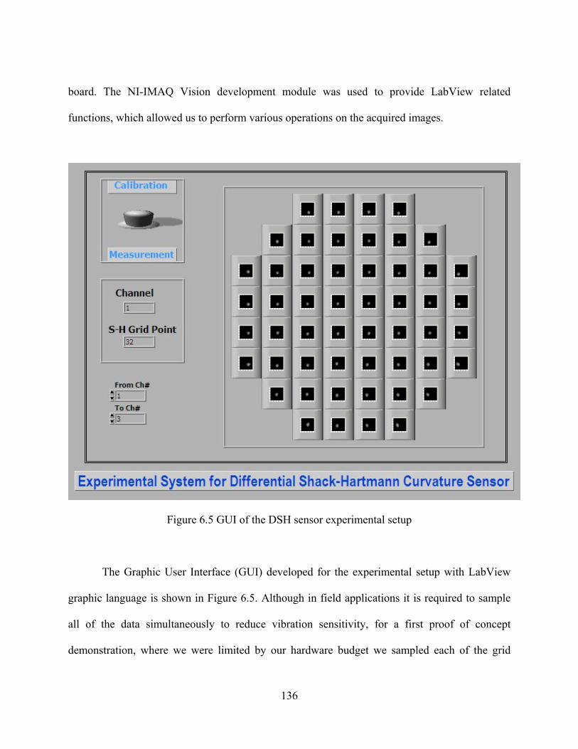
136

board. The NI-IMAQ Vision development module was used to provide LabView related

functions, which allowed us to perform various operations on the acquired images.

Figure 6.5 GUI of the DSH sensor experimental setup

The Graphic User Interface (GUI) developed for the experimental setup with LabView

graphic language is shown in Figure 6.5. Although in field applications it is required to sample

all of the data simultaneously to reduce vibration sensitivity, for a first proof of concept

demonstration, where we were limited by our hardware budget we sampled each of the grid

137

coordinates serially rather than in parallel. An indicator located on the up-left corner of the GUI

shows the sampling process, and the individual images of the 52 Hartmann grid points were

shown in an array on the right side of the GUI according to their original positions. A button

immediately above the process indicator was used to switch between the calibration process and

the measurement process. Once the data was obtained from measurement and calibration,

wavefront estimations were computed with a zonal wavefront estimation algorithm described in

Section 6.4.

6.4 Curvature-based zonal wavefront estimation

Given the wavefront curvature data obtained from the slope differential measurements

and the boundary gradients obtained from slope measurements, the wavefront values may be

estimated. On the basis of wavefront Laplacian curvature measurements inside the pupil and the

slope measurement at the pupil boundary, Roddier and Roddier proposed a zonal iterative FT-

based wavefront estimation algorithm.92 Chanan established a zonal least-squares wavefront

estimation algorithm for curvature data obtained on a square domain.59 In this section, a zonal

least-squares-based estimation algorithm for curvature data based on Taylor series is proposed.

The 8×8 S-H grid used for this experimental system is shown in Figure 6.6. For

convenience, we index the square S-H grid array with the SNS mode (i= 1, 2…m (m=t×t)) as

shown in Figure 5.2. The discretization of Poisson equation yields a normal equation set for the

least-squares-based wavefront estimation (Zou & Rolland 2005).200

For a curvature-based zonal wavefront estimation, the estimation algorithm becomes very

simple because various mathematical frame works needed for estimating the Laplacian

138

curvatures from slope data at each given grid point are avoided. Instead, the Laplacian

curvatures are directly obtained from measurements at each point where the wavefront value is

evaluated, which forces the Southwell geometry, a geometry that yields the best error

propagation in wavefront estimation as detailed in Chapter 5.

Figure 6.6 A 52-point S-H Grid

For any interior point within the sampling domain, the least-squares-based normal

equations for wavefront estimation are always of the same form, which is

( )iyix2

1itiiti1i ccawww4ww ,, +=++−+ ++−− . (6. 6)

For a regular discretization mesh illustrated in Figure 6.6, all the boundary points can be

categorized into two types: the line boundary points and the corner boundary points. As

139

illustrated in Figures 6.7 and 6.8, there are only eight boundary local geometries that are needed

to be taken care of for a given sampling domain. In the following, we will derive the normal

equations for wavefront estimation for each of the eight local geometries.

For the line boundary points illustrated in Figure 6.7(a), the curvature in the x-direction at

this point can be approximated by

ix2

1ii1i caww2w ,=+− −+ . (6. 7)

Figure 6.7 The edge points

In order to couple Poisson equation with the boundary condition, we need to estimate the

boundary slope that is normal to the boundary line. Given the Taylor expansion in the y-

direction, we have

L++−=+ i,y

2

i,yiti c!2

aasww , (6. 8)

where iys , is the slope in the y-direction at point i. If we ignore the higher order terms and add

Eqs. (6.7) and (6.8) together, we obtain the normal equation for the boundary points that shares a

boundary geometry shown in Figure 6.7(a) as

iyiyix2

ti1ii1i asc21cawww3w ,,, −⎟

⎠⎞

⎜⎝⎛ +=++− +−+ . (6.9)

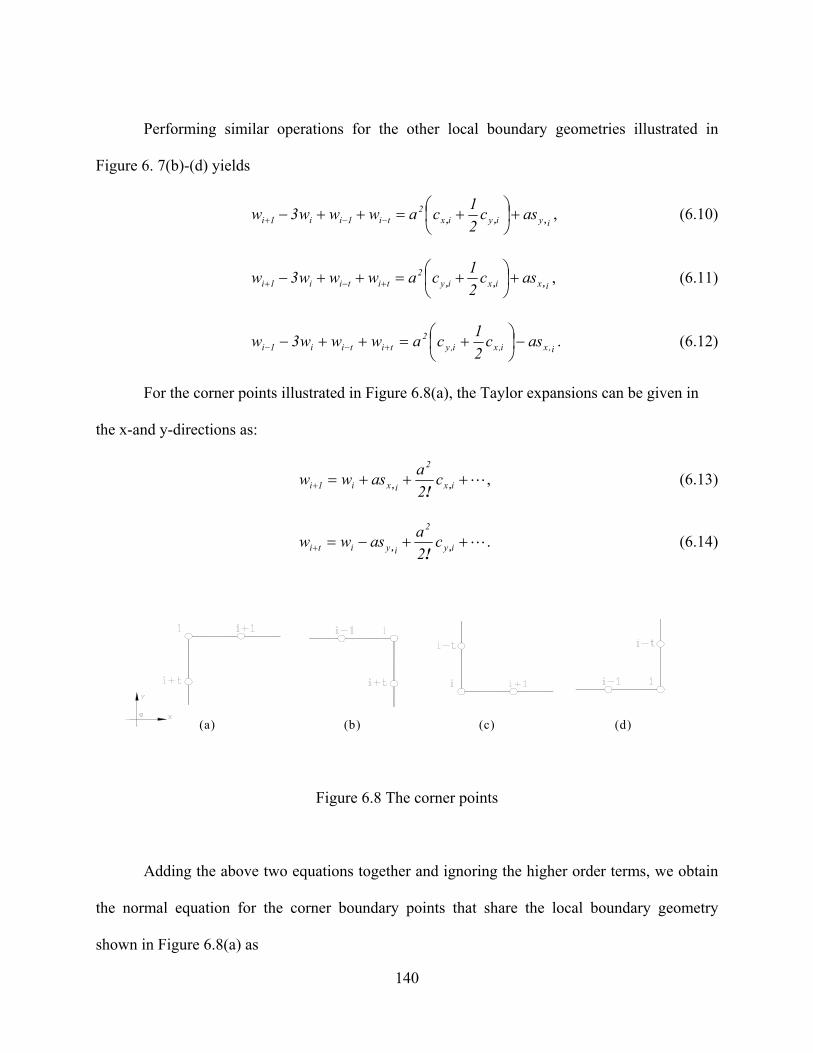
140

Performing similar operations for the other local boundary geometries illustrated in

Figure 6. 7(b)-(d) yields

iyiyix2

ti1ii1i asc21cawww3w ,,, +⎟

⎠⎞

⎜⎝⎛ +=++− −−+ , (6.10)

ixixiy2

titii1i asc21cawww3w ,,, +⎟

⎠⎞

⎜⎝⎛ +=++− +−+ , (6.11)

i,xi,xi,y2

titii1i asc21cawww3w −⎟

⎠⎞

⎜⎝⎛ +=++− +−− . (6.12)

For the corner points illustrated in Figure 6.8(a), the Taylor expansions can be given in

the x-and y-directions as:

L+++=+ ix

2

ixi1i c2aasww ,, !

, (6.13)

L++−=+ iy

2

iyiti c2aasww ,, !

. (6.14)

(a) (b) (c) (d)

Figure 6.8 The corner points

Adding the above two equations together and ignoring the higher order terms, we obtain

the normal equation for the corner boundary points that share the local boundary geometry

shown in Figure 6.8(a) as

141

( ) ( )iyix

2

iyixiti1i cc2

assaw2ww ,,,, ++−=−+ ++ (6.15)

Performing similar operations for the other local boundary geometries illustrated in

Figure 6.8 (b)-(d) yields

( ) ( )iyix

2

iyixiti1i cc2

assaw2ww ,,,, +++−=−+ +− , (6.16)

( ) ( )iyix

2

iyixiti1i cc2

assaw2ww ,,,, +++=−+ −+ , (6.17)

( ) ( )iyix

2

iyixiti1i cc2

assaw2ww ,,,, +++−=−+ −− . (6.18)

Writing the normal equations derived from the interior points and the boundary points in

a proper order, we obtain the normal equation set, which may be expressed in matrix form as

BFAW aa2 −= (6.19)

where A is the normal matrix for zonal wavefront estimation, W is the wavefront vector, a is the

pitch size of the S-H grid, F is the vector of the weighted Laplacian curvature measurements, and

B is a vector of the boundary slopes that are normal to the edge. Compare with the algorithm

obtained by Chanan, they both share the same matrix form. However, their boundary condition

treatments are different, and therefore they are two different algorithms. The validation of this

proposed algorithm is shown in Chapter 7.

Usually the optical surfaces have large errors near the edges. Variations in the boundary

slopes may dramatically change the wavefront estimation results.57 Such a condition makes the

wavefront estimation in optical testing challenging, because the boundary conditions are usually

affected by large edge-slope defects. However, we can not discard the boundary conditions in

wavefront estimation, because it contributes to the wavefront shape besides the wavefront

142

orientation and defocus.47, 87 As detailed in Chapter 3, the orientation of the wavefront is

determined by the boundary slopes only, but the wavefront shape is determined by both the

wavefront Laplacian and the boundary slopes.124

6.5 Principal curvature computations

The normal curvature is the change of the surface normal in an osculating plane, and the

principal curvatures at a non-umbilical point are the maximum and minimum values of the

normal curvatures, say 1κ and 2κ , in two perpendicular directions. Regarding a local patch on a

surface, the principal curvatures are invariants, which are insensitive to the surface orientations.

In order to evaluate the principal curvatures, we assume that the neighborhood of a

Hartmann grid point can be represented by a “Monge patch” of the form:

321 e)y,xW(eyex ++=X (6.20)

where ( 1e , 2e , 3e ) is an orthogonal frame in Euclidean 3-D space. For a wavefront traveling in

the z-direction ( 3e ), W(x,y) is the “height” as a function of x and y in the pupil plane. Then the

second fundamental form has a matrix form to describe the local surface shape as 196

⎟⎟⎠

⎞⎜⎜⎝

⎛

ωωωω

= 232

132

231

131

))

))

II , (6.21)

where 1,2.)j1,2;(i ==3ijω) defines the component in ie of the turning rate of the normal as you

move the frame across the given point along je . Then at each “Monge patch”, the matrix II

becomes

143

m21i(i)c(i)c(i)c(i)c

yxy

yxx ,...,, =⎟⎟⎠

⎞⎜⎜⎝

⎛=II , (6.22)

where the diagonal terms (i)xc and (i)yc are the wavefront normal curvatures in the x-direction

and in the y-direction, i.e. (i)xW(i)c 2

2

x ∂∂

= and (i)yW(i)c 2

2

y ∂∂

= ; the off-diagonal terms (i)cxy and

(i)cyx are the corresponding twist curvature terms, i.e. (i)yx

W(i)c2

xy ∂∂∂

= and (i)xy

W(i)c2

yx ∂∂∂

= .

The determinant of matrix II , denoted as K, is known as the Gaussian curvature, which

measures the total spread of normal directions per unit surface area. 46 The trace of the matrix

II is denoted as 2H, where H is known as the mean curvature, which is the average normal

curvature taken over all tangent directions. Both Gaussian curvature and mean curvature are

algebraic invariants,46 which means they do not change with rotation of the orthogonal frame

( 1e , 2e , 3e ) about the normal.

By diagonalizing the matrix II to rotate the orthogonal frame about 3e , the off-diagonal

terms disappear. Then we obtain a new matrix II ′ by

IIPPII T=′ , (6.23)

where P is an orthogonal matrix defined by

⎥⎦

⎤⎢⎣

⎡ −=

cosθsinθsinθcosθ

P , (6.24)

where the angle θ is defined as the frame rotation angle. The new matrix II ′ is therefore a

diagonal matrix as

⎟⎟⎠

⎞⎜⎜⎝

⎛κ

κ=′

(i)00(i)

2

1II , (6.25)

144

where (i)1κ > (i)2κ (i=1,2, …,m, where m is the total number of the S-H grid points).

(i)1κ and (i)2κ are the eigenvalues of the matrix II , which are also known as the first and second

principal curvatures that define the greatest and smallest normal curvatures at a given patch.

Applying Eqs.(6.22), (6.24) and (6. 25) in Eq.(6.23), we obtain a formula for the principal

curvatures 1κ and 2κ as

( )2

(i)c4(i)c(i)c(i)c(i)c(i)

2xy

2yxyx

1,2

+−±+=κ , (6.26)

and a formula for the rotation angle (i.e. θ is the angle between the first principal curvature and

the x-direction) as

⎟⎟⎠

⎞⎜⎜⎝

⎛

−=θ −

(i)c(i)c(i)c2

tan21(i)

yx

xy1 . (6.27)

The principal curvatures can also be computed by evaluating the eigenvalues of matrix

II with its characteristic equation as

( ) 0det =−κ III , (6.28)

which yields the same result. Additionally, the rotation angle θ can also be computed with the

Euler’s formula (1760) given by 46

[ ](i)(i)(i)H2(i)c2

(i)2cos21

x

κ−κ−

=θ , (6.29)

where H is the mean curvature

( ) 2(i)c(i)c(i)H yx /+= . (6.30)

Then the angle θ is given by

⎟⎟⎠

⎞⎜⎜⎝

⎛κ−κ

−= −

(i)(i)(i)c(i)c

cos21(i)θ

21

yx1 . (6.31)

145

Applying Eq.(6.26) in Eq.(6.31), we have

( ) ⎟⎟⎟

⎠

⎞

⎜⎜⎜

⎝

⎛

+−

−=θ −

2xy

2yx

yx1

(i)c4(i)c(i)c

(i)c(i)ccos

21(i) , (6.32)

which is equivalent to Eq.(6.27).

The principal curvatures and their directions are two important parameters of local

surface shape. We showed how these parameters are estimated directly from the wavefront

Laplacian curvatures and the twist curvature terms with matrix diagonalization method.

6.6 Summary

The DSH curvature sensor is derived from the S-H sensor, so it shares some important

features of the S-H sensor. It is a real-time wavefront sensing, and the measurements are

inherently two-dimensional and parallel. It yields good photon efficiency for all wavelength

bands. The DSH curvature sensor shares some important features of Roddier’s curvature sensor.

Theoretically it is independent of all types of vibrations and drifts, tip/tilts and whole body

movements. Similar to Roddier’s curvature sensor, it is scale tunable by changing the differential

values. After calibration, no external references are needed for all tests.

The DSH curvature sensor has its unique features. (1) Compare with the CGS sensor and

the curvature profiling technique, the DSH curvature sensor provides a more convenient way to

measure the twist curvature terms, while Roddier’s curvature sensor only yields the Laplacian

curvature measurements. The twist curvature terms are important parameters for computing the

principal curvatures and directions, because they provide more information about the exact shape

of the wavefront. (2) The DSH curvature measurements are performed at the pupil of the optical

146

system under test, so the difficulties associated with the operations close to the caustic zone in

Roddier’s curvature sensor are avoided. As pointed out by its inventor, Roddier’s curvature

sensor is valid only for the defocused images taken outside of the caustic zone, inside which the

rays coming from different sample pupil points intersect together.57 Unfortunately the size of the

caustic zone is related with the aberrations of the system under test and the atmospheric

turbulence-induced seeing blur, so there is no general rule to apply.57 (3) The DSH curvature

sensor does not have a 2π-ambiguity problem, while most of the irradiance-based phase retrieval

methods do. This feature makes the DSH curvature sensor work well with large aberrations,

while Roddier’s curvature sensor is good in accuracy only for small aberrations. (4) The DSH

curvature sensor provides a means to remove the need to scan as the profiling curvature sensing

does, and avoids the scan errors and nonlinearity problems.27 As the DSH curvature sensor

measures the curvatures by simultaneously acquiring 2-D slope differentials via three channels, it

is totally insensitive to all types of vibrations and drifts, both in surface height and in surface

slope, so the vibration-induced accuracy degradation is avoided during curvature measurements.

Koenderink pointed out that “it would be better, of course, to sample even higher order

properties of the surface (such as curvature) directly instead of having to infer them from point or

facet samples”. 46 From the normal curvature measurements, we showed how to compute the

principal curvatures and their directions. The principal curvatures contain more shape

information of wavefront than Laplacian curvature, and further more than slope data. Future

work will include review of the mathematical literature for estimating wavefront shape directly

from the principal curvatures and their directions and potentially the development of new

algorithms as well for optical testing instead of the existing Laplacian curvature-based

algorithms.

147

CHAPTER SEVEN: SIMULATION AND ERROR ANALYSIS

In this chapter, we first numerically validate the curvature-based zonal wavefront

estimation algorithm with a test wavefront given by a Zernike polynomial. Then an error analysis

of the DSH sensor is provided.

7.1 Numerical validation of the proposed algorithm

In order to validate the wavefront estimation algorithm proposed in Chapter 6, the

following procedures were adopted. First, a wavefront function was generated as the original

wavefront by using a known Zernike polynomial. Then the first and the second derivatives of

this given wavefront were computed at each grid point. Based on the generated curvature data,

the wavefront was estimated with the proposed algorithm. For evaluating the proposed

wavefront estimation algorithm, the wavefront was also estimated from the generated slope data

with a common iterative wavefront estimation algorithm. This iterative algorithm was used as the

ground truth for evaluating a Gerchberg-Saxton iterative wavefront estimation algorithm in our

previous work presented in Chapter 4.180 Comparisons were made between the original and the

estimated wavefronts. The differences between them were used as metrics for evaluating the

proposed curvature-based algorithm.

The original wavefront function in this simulation was defined by a Zernike polynomial

as

),(ZW),W( 040 θρ=θρ , (7. 1)

148

where ( ) ( )1665,Z 2404 +ρ−ρ=θρ is the term for primary spherical aberration in Zernike

polynomials with π<θ≤≤ρ< 20 10 , , and λ=37W0 . As defined by the Zernike polynomial,

the RMS value of the introduced wavefront is 0W (~2.33λ). If the radius of the wavefront test

pupil is R, then we can write the original wavefront in the Cartesian coordinate form as

( ) ( )⎟⎟⎠

⎞⎜⎜⎝

⎛+

+−

+= 1

Ryx6

Ryx65W)y,xW( 2

22

4

222

0 . (7.2)

Accordingly, the first derivatives (slopes) of the given wavefront can be derived as

( ) ( ) x1R

yx2R

W512y,x

xW

2

22

20

⎟⎟⎠

⎞⎜⎜⎝

⎛−

+=

∂∂ , (7.3)

( ) ( ) y1R

yx2R

W512y,x

yW

2

22

20

⎟⎟⎠

⎞⎜⎜⎝

⎛−

+=

∂∂ , (7.4)

and the second derivatives (curvatures) of the given wavefront can be derived as

( ) ( )⎟⎟⎠

⎞⎜⎜⎝

⎛−

+=

∂∂ 1

Ryx32

RW512

y,xxW

2

22

20

2

2

, (7.5)

( ) ( )⎟⎟⎠

⎞⎜⎜⎝

⎛−

+=

∂∂ 1

Ry3x2

RW512

y,xyW

2

22

20

2

2

. (7.6)

Given the wavefront slope and curvature data on a 8×8 grid (shown in Figure 6.6) by

Eqs.(7.3)-(7.6), we can estimated the wavefront with the zonal curvature-based wavefront

estimation algorithm proposed in Chapter 6. The contour plot of the estimated wavefront from

curvature data is shown in Figure 7.1(a), and the wavefront estimated from slope data is shown

in Figure 7.1(b) for comparison. Both wavefronts were estimated by zonal least-squares

algorithms with the Southwell geometry. Figure 7.1(c) shows the original wavefront with the

149

8×8 discretization grid. In Figures 7.1 and 7.2, the “Ave” stands for the mean value of the

wavefront, and the “Var” stands for the RMS value of the wavefront.

-1 -0.5 0 0.5 1-1

-0.8

-0.6

-0.4

-0.2

0

0.2

0.4

0.6

0.8

1

-2

-2 -2

-2

-2

-2-2 -2

-2

-2

-2

-2

-2

-2

-2

0

0

0

0

0

0

00

0

0

0

0

0

0

0

0

2 2

2

2

4

44

6

6

Curvature-based WFE(8x8), Ave= 0.000 wave,Var= 2.472 wave

-1 -0.5 0 0.5 1-1

-0.8

-0.6

-0.4

-0.2

0

0.2

0.4

0.6

0.8

1

-2

-2

-2

-2

-2 -2

-2

-2-2

-2

-2

-2

0

0 0

0

0

0

0

0

0

0

0

0

0

2

2

2

2

2

2

2

2

2

22

Slope-based WFE(8x8), Ave=-0.000wave,Var= 2.210wave

-1 -0.5 0 0.5 1

-1

-0.8

-0.6

-0.4

-0.2

0

0.2

0.4

0.6

0.8

1

-2

-2-2

-2

-2

-2

-2

-2

-2

-2

-2

-2

-2

0

0

00

0

0

0

0

0

0

0

0

0

0

0

02

2

2

2

2

2

2

2

2

2

2

4

4

Original Wavefront(8x8) Ave= 0.000 wave,Var= 2.154 wave

(a) (b) (c)

-1 -0.5 0 0.5 1-1

-0.8

-0.6

-0.4

-0.2

0

0.2

0.4

0.6

0.8

1

-1

-1

-1

-1

-1

-1-1

-1

-1-1

-1-1-1

-1 -1-1-1

0

0

00

0

0

0

0

0

0

0

00

0

0

0

0

1

1

1

1

1 2

Curvature-based WFD(8x8), Ave= 0.000wave,Var= 1.144wave

-1 -0.5 0 0.5 1-1

-0.8

-0.6

-0.4

-0.2

0

0.2

0.4

0.6

0.8

1

-0.8

-0.8

-0.8

-0.4

-0.4

-0.4

-0.4

-0.4

0

00

0

0 0

0

0.4

0.4

0.4

0.4

0.4

0.4

0.4

0.4

0.4

0.4

0.4

0.40.4

0.40.4

0.40.4

Slope-based WFD(8x8), Ave=-0.000wave,Var= 0.572wave

(d) (e)

Figure 7.1 Wavefront estimation with an 8×8 grid array

(a) Estimated wavefront from curvature data. (b) Estimated wavefront from slope data.

(c) Original wavefront on an 8×8 grid. (d) Deviation error map of the estimated wavefront from

curvature data. (e) Deviation error map of the estimated wavefront from slope data.

The difference between the estimated wavefront and the original wavefront is referred to

150

as the wavefront deviation error of the proposed wavefront estimation. The wavefront RMS

deviation error is defined as the root-mean-square value of the difference between the two

wavefronts at each grid point. The RMS value of the curvature-based wavefront is 2.47λ

(λ=632.8nm for this chapter), the RMS value of the slope-based wavefront is 2.21λ, and the

RMS value of the original wavefront is 2.51λ. The wavefront deviation error maps generated by

the curvature-based and slope-based wavefront estimations are shown in Figures 7.1(d) and (e),

which are shown to have RMS deviation errors of 1.144λ and 0.572λ, respectively.

It can be observed that the coarse grid sampling is the main cause of the large deviation

RMS errors. To get insight into the impact of the grid sampling size on the deviation error when

the exit pupil is fixed, we provide another simulation example of wavefront estimation with a

30×30 grid array in Figure 7.2. The estimated wavefronts from curvature and slope data are

shown in Figure 7.2(a)-(b), and the original wavefront with the 30×30 grid array is shown in

Figure 7.2(c). The RMS value of the curvature-based wavefront is 2.387λ, the RMS value of the

slope-based wavefront is 2.392λ, and the RMS value of the original wavefront is 2.390λ. The

corresponding wavefront deviation error maps of the curvature and slope-based wavefront

estimations are shown in Figure 7.2(d)-(e), in which the RMS deviation errors are 0. 081λ and

0.041λ, respectively.

For both examples if we decompose the estimated wavefronts into the Zernike

polynomials (for t>5), a spherical aberration of 2.33λ(~7/3λ) can be retrieved, which is the

original aberration value that was introduced by Eq. (7.2). This provides a validation of the

curvature-based zonal wavefront estimation algorithm proposed in this dissertation.

151

-1 -0.5 0 0.5 1-1

-0.8

-0.6

-0.4

-0.2

0

0.2

0.4

0.6

0.8

1

-2

-2

-2

-2

-2-2

-2

-2-2

-2

-2

-2

-2

0

0 00

0

00

0

00

00

2

2

2

22

2

2

22

2

2

2

2

22

2

2

22 2

2

2

2

4

4

4

4

4

4

44

4

4

4

4

44

4

4

4

4

4

4

4

4

4

4

Curvature-based WFE(30x30), Ave=-0.000 wave,Var= 2.387 wave

-1 -0.5 0 0.5 1-1

-0.8

-0.6

-0.4

-0.2

0

0.2

0.4

0.6

0.8

1

-2

-2 -2

-2

-2

-2

-2

-2

-2

-2

-2

-2

-2

0

00

0

0

0

0

0

0 0

00

2

2

22

2

2

2

2

2

2

2

2

2

2

2 22

2

2

2

2

2

4

4

4

4

4

4

4

4

4

4

4

4

444

4

4

4

4

4

4

4

4

4

Slope-based WFE(30x30), Ave= 0.000wave,Var= 2.392wave

(a) (b) (c)

-1 -0.5 0 0.5 1-1

-0.8

-0.6

-0.4

-0.2

0

0.2

0.4

0.6

0.8

1

-0.1

-0.1

-0 1-0.1

-0.1

-0.1

-0.1

-0.1

-0.1

-0.1

-0.1

-0.1-0

.1

-0.1

-0.1-0.1-0.1

-0.1

0

0

00

0

0

0

0

0

0 0

00

0

00

0

0.1

0.1

0.1

0.1

Curvature-based WFD(30x30), Ave=-0.000wave,Var= 0.081wave

-1 -0.5 0 0.5 1-1

-0.8

-0.6

-0.4

-0.2

0

0.2

0.4

0.6

0.8

1

-0.04

-0.04

-0.04

-0.04

0

0 0

0

00

00.04

0.04

0.040.04

0.04

0.04

0.04

0 04

0.04

004

0.04

0.04 0.04

0.04

0.04

0.040.04

0.04

Slope-based WFD(30x30), Ave=-0.000wave,Var= 0.041wave

(d) (e)

Figure 7. 2 Wavefront estimation with 30×30 grid array

(a) Estimated wavefront from curvature data. (b) Estimated wavefront from slope data.

(c) Original wavefront on a 30×30 grid. (d) Deviation error map of the estimated wavefront from

curvature data. (e) Deviation error map of the estimated wavefront from slope data.

Further study shows that the deviation error of the slope-based wavefront is only half that

of the curvature-based wavefront, as shown in Figure 7.3, and both of them decrease

exponentially with an increase in the sampling grid size. After removal of the piston error and

the tip/tilt error in the estimated wavefront, we found that the deviation error in the estimated

-1 -0.5 0 0.5 1-1

-0.8

-0.6

-0.4

-0.2

0

0.2

0.4

0.6

0.8

1

-2

-2

-2

-2

-2-2

-2

-2

-2

-2

-2

-2

-2

0

0 0

0

0

00

0

00

0

0

2

2

22

2

2

2

2

2

2

2

2

2

2

2 2

22

2

2

2

2

4

4

4

4

4

4

4

4

4

4

4

4

44

4

4

4

4

4

4

4

4

4

4

Original W avefront(30x30) Ave=-0.000 wave,Var= 2.390 wave

152

wavefront is mainly the defocus value (>98%). In Figure 7.3, curves 1 and 2 are the plots of the

deviation errors of the curvature-based and slope-based wavefront estimations versus the grid

size, and the curves 3 and 4 are the plots of the corresponding defocus values. It is interesting to

notice that the defocus value in the curvature-based estimation is twice that of the slope-based

estimation but of different sign. As shown in Figure 7.3, the curvature-based defocus value is

negative, while the slope-based defocus value is positive.

5 8 10 20 30 40-2

-1

0

1

2

WFE

dev

iatio

n er

ror &

defo

cus(

in w

avel

engt

h)

Grid size

1.Curvaure-based deviation error(RMS) 2. Slope-based deviation error(RMS) 3. Curvature-based defocus 4. Slope-based defocus1

2

3

4

Figure 7. 3 Wavefront deviation errors and the defocus values

The RMS value of the discretized original wavefront is the RMS value of the true

wavefront values computed on the whole grid. Although the RMS wavefront deviation error is

defined as the RMS difference between the estimated wavefront value and the original wavefront

value at each grid point, the RMS value of the discretized original wavefront differs from the

RMS value of the continuous true wavefront (which is 7λ/3 in this example) as a result of

wavefront discretization. The difference between the two RMS wavefront values is defined as

153

the wavefront discretization error. As shown in Figure 7.4, the discrete sampling becomes

denser as the grid size increases, and the wavefront discretization error tends to zero.

In the above numerical simulations, the pupil size is about 15mm in diameter, which

corresponds to an 8×8 grid array with a pitch size of 1.79mm. When the grid size is increased,

the pitch size of the S-H grid decreases for a fixed pupil. For the case of a 40×40 grid size (the

maximum grid size in simulation), the pitch size of the S-H grid is 0.36mm.

0 10 20 30 40 501.5

2.0

7/3

2.5

3.0

Wav

efro

nt d

iscr

etiz

atio

n er

ror (

in w

avel

engt

h)

Size of discretization grid array t

Figure 7. 4 Wavefront discretization error versus discretization grid size

7.2 Error analysis of wavefront measurement

Because the DSH curvature sensor is based on the S-H sensor, its measurement capability

is limited by the dynamic range of the S-H sensor in each channel, while its measurement

accuracy is limited by the sensitivity of the S-H sensor in each channel. We shall provide an

analysis of dynamic range and sensitivity, and exemplify this analysis using spherical aberration

154

as the departure aberration from an ideal shape. The dynamic range and sensitivity will be

computed in both slope values and number of waves of wavefront departure utilizing the

experimental setup parameters given in Chapter 6.

For a wavefront with third-order spherical aberration of 040W , we have

( )2224

0404040 yx

RW

W)y,x(W +=ρ= . (7.7)

where R is the pupil radius at the optics under test (e.g. a mirror), and 10 ≤ρ≤ is the

normalized pupil radius, and x and y in Eq. (7.7) are physical dimensions within the pupil.

Differentiating Eq. (7.7) yields wavefront slopes in the x-and y-direction as

( ) ( )xyxRW4

y,xxWS 22

4040

x +=∂∂

= , (7.8)

( ) ( )yyxRW4

y,xyWS 22

4040

y +=∂∂

= . (7.9)

7.2.1 Dynamic range

The dynamic range is defined as the largest wavefront slope that can be measured. Given

that the pitch size of the lenslet array is 1.79mm, and the focal length of the lenslet array is

90mm, the maximum slope that the lenslet array can sense can be determined by

,radian 00994.0)902/(79.1tan max ≈×=θ (7.10)

so the dynamic range of the S-H sensor is o57.0max ±=θ , which corresponds to a local wavefront

slope error of 35.3D/dmax ′±=θ arc minutes at the mirror surface, where d=15mm is the exit

pupil size at the lenslet and the D=152.4mm is the mirror size.

155

In expressing this slope error in terms of the wave number of wavefront error, we shall

note that spherical aberration displays its largest amount of slope value at the edge of the pupil,

and the aberration is rotationally symmetric. Thus considering the edge of the mirror pupil in the

x-direction (i.e. x=R=76.2mm, y=0), we establish that

λ≈=×

××=

θ== 29.5 mm0186.0

152.4 4 76.2 15 0.00994

D4R d

x 4RS

W max3

4x

040 , (7.11)

where the λ equals 0.6328nm. Thus the dynamic range at the mirror is quantified to be in slope

measurements ± 35.3′ arc minutes or in wavefront amplitudes about ± 30 waves.

7.2.2 Sensitivity

The sensitivity of a S-H sensor is defined as the smallest slope data that can be measured.

Assuming that a S-H spot centroid position can be acquired with an accuracy of one tenth of a

pixel size when a high quality camera is used, the smallest measurable slope value is

f CCD

min βσ

=θ (7.12)

where 3.2/1=β is the magnifying power from the lenslet array image plane to the CCD

camera, and mm90f = is the focal length of the lenslet array. Assuming a CCD camera with 8.4

μm pixel size, then

secarc4.4radian10147.290mm /3.2mm10 84.0 5-3min =×=××=θ − , (7.13)

which corresponds to a wavefront slope error at mirror surface of secarc43.0D/dminM =θ=θ .

156

To estimate the smallest value of 040W that can be measured, we consider the edge of the

mirror pupil in the x-direction (i.e. x=R=76.2mm, y=0), where the wavefront have its maximum

slope

RW4

S 040max = , (7.14)

To make the wavefront sensible for the S-H sensor, the maximum wavefront slope maxS should

be at least as big as the smallest measurable slope value Mθ , and then we establish that

λ≈μ=×

×××=

θ=

−

0636.0m04.0mm4.1524

mm15mm2.7610147.2D4RdW

5min

040 (7.15)

where the λ equals 0.6328nm. The above analysis shows that given a RMS CCD centroiding

error of 101 pixel, λ/15 is the smallest third-order spherical aberration (P-V) that our

experimental system can sense, and 0.43 arc sec is the smallest wavefront slope value sensible at

the mirror surface. It is to be noted that the accuracy of the CCD camera, along with the quantity

of the S-H spots, drives the magnitude of the slope measurement error. Therefore, based on the

special requirement for testing applications, a high performance CCD is desirable.

7.2.3 Accuracy

In the following, we will show how much wavefront measurement accuracy that an S-H

sensor of the DSH experimental system can achieve, when the error propagation in wavefront

estimation is considered. For the Laplacian curvature-based wavefront estimation, either the

Fried geometry or the Southwell geometry can be applied. Because of its convenience for

wavefront estimation and its low error propagation behavior, the Southwell geometry was

157

adopted in our work. For the slope-based wavefront estimation in each channel, the error

propagation coefficient was given in Chapter 5 by

SS2s

2w

S ηKσση ==′ (7.16)

where ( ) 00 A8750mtmAK ./ =−=S for the Southwell geometry. 0A is the pitch area of the

sampling grid, and Sη is the WFD-based error propagation coefficient defined by Eq.(5.36) and

estimated by Eq.(5.39). For a 8 ×8 sampling grid,

1.1387)t(ln0.410.2861ηS =+= , (7.17)

thus 00S A9963.01387.1A875.0η =×=′ . Therefore, the mean variance of the wavefront

estimation error is given as

2s0

2s

2w A9963.0ησ σ=σ= ′S . (7.18)

Since the equally spaced sampling grid is square, and its pitch area is 20 aA = , then Eq. (7.18)

yields

fa

9963.0ησ CCDsw β

σ=σ= ′S . (7.19)

Therefore, the RMS wavefront estimation error with an 8 ×8 sampling grid can be estimated by

λ=μ=×μ×

×= 0.061m0384.0mm90

3.2m84.0mm79.19963.0σw , (7.20)

where λ equal to 632.8nm.

The analysis shows that if the RMS wavefront slope measurement error of an S-H sensor

is 1/10 pixel, the RMS wavefront estimation error will be λ/16. Since the wavefront estimation

158

error is driven by both the pitch size of the sampling grid and the CCD centroiding accuracy, a

smaller wavefront estimation error may be obtained if a smaller grid size is adapted.

7.3 Summary

In this chapter, we validate the accuracy of the zonal curvature-based wavefront

estimation algorithm presented in Chapter 6. We provide an analysis of the dynamic range, the

instrument sensitivity, and the wavefront estimation accuracy of the DSH curvature experimental

system under development. As part of the lessons learned, the camera we considered for

methodology development was found to have dead space in one direction which resulted in data

missing during measurements, thereby a low CCD centroiding accuracy. A high performance

CCD camera will be necessary for the application of optical testing where wavefront estimation

at level of λ/4~λ/100 may be required.

159

CHAPTER EIGHT: SUMMARY OF CONTRIBUTIONS AND CONCLUSION

With developments in active and adaptive optics, ophthalmology, and optical shop testing

wavefront sensing has become increasing prevalent. Wavefront sensing can involve either direct

or indirect OPD measurements. This dissertation focused on indirect OPD sensing, specifically

the parameter-based wavefront sensing. Three major contributions were made for optimizing

wavefront sensing techniques. First, an iterative zonal wavefront estimation algorithm for any

irregular pupil shape was presented;180 secondly, a theoretical study of error propagation for

zonal wavefront estimations was performed;190 thirdly, a differential Shack-Hartmann curvature

sensor was proposed and implemented.194

For parameter-based wavefront sensing, either wavefront slope or wavefront curvature or

a combination are measured within the pupil under test. One problem encountered in the slope-

based wavefront estimation is how to handle wavefront estimation with irregular pupil shapes.

In optical shop, optical elements can be round, square, or circular but with central obscuration,

etc. A zonal wavefront estimation algorithm was proposed based on a least-squares linear

equation system and Gerchberg-Saxton iterations. A domain extension technique was used to

transform the irregular pupil into a square shape, and a serial numbering scheme was adopted for

indexing the sampling grid inside the square domain to make the wavefront estimation matrix

regular, symmetric and pre-defined. Gerchberg-Saxton iterations were employed to extrapolate

the slope data outside the original pupil. The deviation error induced in the wavefront domain

extension was then reduced to less than λ/100, and the convergence was showed to occur within

a few iterations. It is believed to be the first implementation of the Gerchberg-Saxton algorithm

160

with a least-squares linear system technique. The strength of the approach lies in the fact that the

least-squares-based Gerchberg-Saxton algorithm does not suffer from the 2π-phase ambiguity

problem commonly encountered in Fourier-based approaches. As a result the least-squares-based

Gerchberg-Saxton algorithm is superior for estimating large aberrations. A theoretical analysis

shows that this algorithm is not only computationally efficient but also yields low error

propagation.

Error propagation is an important parameter in evaluating slope-based wavefront

estimation. Based on the serial numbering scheme, wavefront estimation matrices for the

Hudgin, Southwell and Fried geometries were established. It was shown that the error

propagation coefficient can be expressed as a function of the eigenvalues of the wavefront-

estimation-based matrix, where the error propagation behavior differs with the different parity of

the grid size. For wavefront estimation with a “zero point” chosen, odd-number grid sizes were

shown to be preferable to even-number grid sizes. This formulation confirms Noll’s theoretical

result if the Southwell geometry is adopted with the odd-number grid sizes.

From the wavefront difference-based wavefront estimation to the wavefront slope-based

wavefront estimation, if the effect of the pitch size is not considered, the error propagator does

not change much for the Hudgin and the Southwell geometries, but it becomes four times worse

for the Fried geometry. In sum, the Southwell geometry is recommended as the best error

propagator for both the difference-based and slope–based wavefront estimations.

For curvature-based wavefront estimation, a differential Shack-Hartmann (DSH)

curvature sensor was proposed, which measures wavefront curvatures by measuring the

differentials of the wavefront slopes at each Shack-Hartmann grid point in parallel. An

161

algorithm for zonal wavefront estimation from curvature measurements was proposed and

demonstrated. For slope differential measurements at each S-H grid point, the Southwell

geometry has been demonstrated to be the best choice. The curvature-based wavefront estimation

algorithm was shown to be equivalent to the slope-based wavefront estimation algorithm for the

Southwell geometry, but it is much simpler and more convenient to apply. Furthermore,

curvature data acquired by the DSH sensor is expected not to suffer from vibration induced

noise, a current limitation of most slope-based sensors and some curvature sensors.

The principal curvatures and their directions are two important parameters in

characterizing the wavefront local shape, which are the maximum and minimum curvatures of

any local patch on the surface in two orthogonal directions. It is known that the principal

curvatures can be computed from the Laplacian curvatures and the twist curvature terms. We

provide in this dissertation a means with the DSH sensor to measure such components for the

first time. Previous curvature sensors essentially focused on measuring solely the Laplacian

curvatures, which is not sufficient to compute the principal curvatures and directions of a local

patch for describing the local wavefront shape.

The main merits of the DSH sensor are its immunity to vibrations, its ability to better

measure the twist curvature terms, and its capability with high sampling to estimate the mid-

spatial frequency error as well as the low-spatial frequency, which move the wavefront sensing

technique to the next level of profilometry accuracy. Finally, with efficient two-dimensional

curvature measurements in parallel, the problems associated with one-dimensional point-by-

point-scan curvature profiling are avoided.

162

Future work will involve the comprehensive engineering investigation of the DSH sensor

for various applications. The design of the instrument will differ based on the requirements for

sensitivity and dynamic range. In developing any DSH instrument, care will need to be taken in

easing the alignment of the three channels and minimizing spurious aberrations introduced by

components that make up the system. It is also of interest to investigate algorithms for wavefront

estimation directly from the principal curvatures and directions and yield insight into the ability

of this parameterization to best represent overall local and global shape. Finally, any departure

in estimated shape from a defined gold standard should be correlated to the impact of such errors

on the performance metrics of various tasks linked to specific applications.189

163

APPENDIX DERIVATION OF EQS. (4.11), (4. 12), (4.26) AND (4. 27)

164

(on page 79, 79, 81 and 81, respectively)

The nth derivative of the wavefront at point i is denoted as i

n

n

yW

∂∂ , and the nth derivative

of the wavefront at the midpoint between the points i and i+1 as 21i

n

n

yW

+∂∂ . According to Taylor’s

series, we can write

)Ο(ayW

!416a

yW

!38a

yW

!24a

yW

2aww 5

i4

44

i3

33

i2

22

iii

21

21

21

21

21 +

∂∂

×+

∂∂

×−

∂∂

×+

∂∂

−=++++

+ , (A1)

and

)Ο(ayW

!416a

yW

!38a

yW

!24a

yW

2aww 5

i4

44

i3

33

i2

22

ii1i

21

21

21

21

21 +

∂∂

×+

∂∂

×+

∂∂

×+

∂∂

+=++++

++ . (A2)

Subtracting Eq.(A1) from Eq.(A2) yields

)a(yW

!34a

yWaww 5

i3

33

ii1i

21

21

Ο+∂∂

×+

∂∂

=−++

+ . (A3)

Adding Eq.(A1) and Eq.(A2) yields

)a(yW

!48a

yW

4aw2ww 6

i4

44

i2

22

ii1i

21

21

21 Ο+

∂∂

×+

∂∂

+=+++

++ . (A4)

Replacing w withy

W∂∂ in (A4) yields

)a(yW

!48a

yW

4a

yW2

yW

yW 6

i5

54

i3

32

ii1i21

21

21

Ο+∂∂

×+

∂∂

+∂∂

=∂∂

+∂∂

++++

. (A5)

Ignore the high order terms in (A5), we have

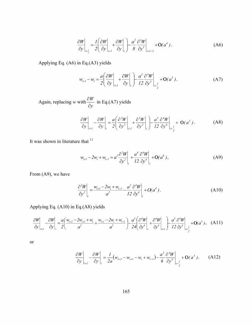
165

)a(yW

8a

yW

yW

21

yW 4

2/1i3

32

i1ii 21

Ο+∂∂

−⎟⎟⎠

⎞⎜⎜⎝

⎛

∂∂

+∂∂

=∂∂

+++

. (A6)

Applying Eq. (A6) in Eq.(A3) yields

)a(yW

12a

yW

yW

2aww 5

21i

3

33

i1ii1i Ο+

∂∂

−⎟⎟⎠

⎞⎜⎜⎝

⎛

∂∂

+∂∂

=−++

+ . (A7)

Again, replacing w withyW∂∂ in Eq.(A7) yields

)a( yW

12a

yW

yW

2a

yW

yW 5

21i

4

43

i2

2

1i2

2

i1i

Ο+∂∂

−⎟⎟⎠

⎞⎜⎜⎝

⎛

∂∂

+∂∂

=∂∂

−∂∂

+++

. (A8)

It was shown in literature that 11

)a(yW

12a

yWaww2w 6

i4

44

i2

22

1ii1i Ο+∂∂

+∂∂

=+− −+ , (A9)

From (A9), we have

)a(OyW

12a

aww2w

yW 4

i4

42

21ii1i

i2

2

+∂∂

−+−

=∂∂ −+ . (A10)

Applying Eq. (A10) in Eq.(A8) yields

)a(yW

12a

yW

yW

24a

aww2w

aww2w

2a

yW

yW 5

21i

4

43

1i4

4

i4

43

21ii1i

2i1i2i

i1i

Ο+∂∂

−⎟⎟⎠

⎞⎜⎜⎝

⎛

∂∂

+∂∂

−⎟⎠

⎞⎜⎝

⎛ +−+

+−=

∂∂

−∂∂

++

−+++

+

, (A11)

or

( ) )a( yW

6awwww

a21

yW

yW 5

21i

4

43

1ii1i2ii1i

Ο+∂∂

−+−−=∂∂

−∂∂

+

−+++

. (A12)

166

If we neglect the higher order small-value terms on the right side of Eq. (A12) and denote

the first derivative of the wavefront in the y-direction as sy, then Eq.(12) becomes

( )i1i2i3i1y i2y i w-ww wa2

1ss +−=− +++++ , (A13)

where i=1,2,… t-3; t+1,t+2,… 2t-3, …m-3.

Similarly in the z-direction, we can write

( )t3it2itiit2z, itz, i w-ww wa2

1ss +++++ +−=− , (A14)

where i=1,2,…t, t+1,t+2,…2t,…, m-3t.

167

LIST OF REFERENCES

1. D. Malacara, “Chapter 30 Optical testing”, in Michael Bass (editor in chief), “Handbook of

Optics II”, “Device, measurements and properties”, McGRAW-Hill, INC.(1995).

2. D. E. Vandenberg, W. D. Humbel and A. Wertheimer, “Quantitative evaluation of optical

surfaces by means of an improved Foucault test approach”, Optical Engineering, Vol.32,

No.8, pp.1951-1954 (1993).

3. A. S. DeVany, "Spherical aberration analysis by double wire testing”, Appl. Opt. 6, 1073-

(1967).

4 . J. Ojeda-Castaneda, “Foucault, Wire, and Phase modulation Tests”, in “Optical Shop

Testing” (2nd edition), D. Malacara Ed., 265-313, John Wiley &Sons, Inc (1992).

5. R. Platzeck and E. Gaviola, “On the errors of testing and a new method for surveying optical

surfaces and systems”, J. Opt. Soc. Am. 29, pp.484-500 (1939).

6. I. H. Schroader, “The caustic test”, in Amateur Telescope Making III, A. G. Ingalls, ed.,

pp.429-456, Kingsport Press (1953).

7. D. Banerjee, R. Willstrop, and B. Anandarao, “Improving the accuracy of the caustic test”,

Appl. Opt., Vol. 37, No. 7, pp.1227-1230 (1998).

8. M. Born & E. Wolf, “Principle of Optics” (2nd edition), Sec. 5.1, Pergamon Press, New York

(1964).

168

9. I. Ghozeil, “Hartmann and other screen tests”, in “Optical Shop Testing” (2nd edition.), D.

Malacara Ed., pp.367-392, John Wiley &Sons, Inc. (1992).

10. R. V. Shack and B. C. Platt, “Production and use of a lenticular Hartmann screen”, J. Opt.

Soc. Am. 61, p656 (abstract only) (1971).

11. W. Zou and Z. Zhang, “Generalized wavefront reconstruction algorithm applied in a Shack-

Hartmann test”, Appl. Opt., Vol. 39, No.2, 250-268 (2000).

12. R. Ragazzoni, “Pupil plane wavefront sensing with an oscillating prism,” J. Modern Opt.

43(2), 289-293 (1996).

13. S. Esposito and A. Riccardi, “Pyramid Wavefront Sensor behavior in partial correction

Adaptive Optic systems”, Astronomy and Astrophysics, Vol.369, L9-L12 (2001).

14. B. J. Bauman, “Optical design for Extremely Large Telescope adaptive optics system”,

Chapter 3, PhD dissertation, University of Arizona (2003).

15. R. Ragazzoni and J. Farinato, “Sensitivity of a pyramidic Wavefront sensor in closed loop

Adaptive Optics,” Astronomy and Astrophysics, Vol. 350, L23–L26, (1999).

16. A.A Michelson and E.W Morley, “On the Relative Motion of the Earth and Luminiferous

Ether”, American Journal of Science, 34, 333-345 (1887).

17. P. Hariharan, “Chapter 21 Interferometers”, in Michael Bass (editor in chief), “Handbook of

Optics II”, “Device, measurements and properties”, McGRAW-Hill INC (1995).

18. J. W. Hardy and A. J. MacGovern, “Shearing interferometry: a flexible technique for

wavefront measurement”, in Interferometric Metrology, Proc. SPIE 816 (1987).

169

19. C. Elster and I. Weingrtner, "Solution to the Shearing Problem," Appl. Opt. 38, 5024-5031

(1999).

20. A. Dubra, C. Paterson, and C. Dainty, "Wave-front reconstruction from shear phase maps by

use of the discrete Fourier transform," Appl. Opt. 43, 1108-1113(2004).

21 . M. V. R. K. Murty, “The use of a single plane parallel plate as a lateral shearing

interferometer with a visible gas laser source”, Appl. Opt. 3, 531-534 (1964).

22. J. E. Greivenkamp and J. H. Bruning, “Phase shifting interferometry”, in “Optical Shop

Testing” (2nd edition), D. Malacara Ed., 501-753, John Wiley &Sons Inc (1992).

23. R. Crane, “Interference Phase Measurement," Appl. Opt. 8, 538- (1969).

24. J. H. Bruning, D. R. Herriott, J. E. Gallagher, D. P. Rosenfeld, A. D. White, and D. J.

Brangaccio, "Digital wavefront measuring interferometer for testing optical surfaces and

lenses," Appl. Opt. 13, 2693- (1974).

25. C. Wyant, "Use of an ac heterodyne lateral shear interferometer with real-time wavefront

correction systems," Appl. Opt. 14, 2622- (1975).

26. O. Kafri, "Fundamental limit on accuracy in interferometry," Opt. Lett. 14, 657- (1989).

27. P. Glenn, “Robust, sub-Angstrom lever mid-spatial frequency profilometry”, Advanced

Optical Manufacturing and Testing, Proc. SPIE 1333, 230-238 (1990).

28. I. Weingaertner and M. Schulz, “High-accuracy interferometric measurement of aspheres”,

in Interferometry XI: Applications, Proc. SPIE 4778, 105-118 (2002).

29. J. W. Goodman, Statistical Optics, Sec. 3.3, Wiley, New York (1985).

170

30. B. M. Levine, E. A. Martinsen, A. Wirth, A. Jankevics, M. Toledo-Quinones, F. Landers,

and T. L. Bruno, "Horizontal Line-of-Sight Turbulence Over Near-Ground Paths and

Implications for Adaptive Optics Corrections in Laser Communications ," Appl. Opt. 37,

4553-4560 (1998).

31. B. H. Dean and C. W. Bowers, "Diversity selection for phase-diverse phase retrieval ," J.

Opt. Soc. Am. A 20, 1490-1504 (2003).

32. A. Miks and J. Novak, "Analysis of imaging properties of a vibrating thin flat mirror," J.

Opt. Soc. Am. A 21, 1724-1729 (2004).

33. A. Stern and N. S. Kopeika, "Optical transfer function analysis of images blurred by

nonharmonic vibrations characterized by their power spectrum density," J. Opt. Soc. Am. A

16, 2200-2208 (1999).

34. A. Stern and N. S. Kopeika, "Analytical method to calculate optical transfer functions for

image motion and vibrations using moments ," J. Opt. Soc. Am. A 14, 388- (1997).

35. J. Pfund, N. Lindlein, and J. Schwider, "Misalignment effects of the Shack -Hartmann

sensor ," Appl. Opt. 37, 22-27 (1998).

36. C. Curatu, G. Curatu, and J. Rolland, "Tolerance analysis method for Shack-Hartmann

sensors using a variable phase surface," Opt. Express 14, 138-147 (2006).

37. P. J. de Groot, "Vibration in phase-shifting interferometry," J. Opt. Soc. Am. A 12, 354-

(1995).

171

38. P. L. Wizinowich, "Phase shifting interferometry in the presence of vibration: a new

algorithm and system," Appl. Opt. 29, 3271- (1990).

39 . L. Deck, "Vibration-resistant phase-shifting interferometry," Appl. Opt.35, 6655-6662

(1996).

40. K. J. Barnard, C. E. White, and A. E. Absi, "Two-Dimensional Restoration of Motion-

Degraded Intensified CCD Imagery," Appl. Opt. 38, 1942-1952 (1999).

41. P. D. Ruiz, J. M. Huntley, Y. Shen, C. R. Coggrave, and G. H. Kaufmann, "Vibration-

Induced Phase Errors in High-Speed Phase-Shifting Speckle-Pattern Interferometry ," Appl.

Opt. 40, 2117-2125 (2001).

42 B. K. A. Ngoi, K. Venkatakrishnan, and N. R. Sivakumar, "Phase-Shifting Interferometry

Immune to Vibration," Appl. Opt. 40, 3211-3214 (2001).

43. C. Zhao and J. H. Burge, "Vibration-Compensated Interferometer for Surface Metrology,"

Appl. Opt. 40, 6215-6222 (2001).

44. J. M. Huntley, "Suppression of phase errors from vibration in phase-shifting interferometry,"

J. Opt. Soc. Am. A 15, 2233-2241 (1998).

45. M. Milman, "Optimization approach to the suppression of vibration errors in phase-shifting

interferometry," J. Opt. Soc. Am. A 19, 992-1004 (2002).

46. J. J. Koenderink, “Solid shape”, p210, p214, p228, p212, p232, the MIT press, Cambridge,

Massachusetts (1990).

172

47. F. Roddier, “Curvature sensing and compensation: a new concept in adaptive optics,” Appl.

Opt. 27, 1223–1225(1988).

48. Daniel Malacara, Manuel Servin and Zacarias Malacara, “Interferogram analysis for optical

testing”, p368, p372, 373, Marcel Dekker, Inc.(1998).

49. R. Kupke, F. Roddier and D. Mickey, “Curvature-based wavefront sensor for use on

extended patterns”, in Adaptive Optics in Astronomy, Proc. SPIE 2201, 519-527(1994).

50. R. Kupke, F. Roddier and D. Mickey, “Wavefront curvature sensing on extended arbitrary

scences: simulation results”, in Adaptive optical system technologies, Proc. SPIE 3353-41,

Kona, Hawaii (1998).

51. M. R. Teague, "Irradiance Moments:Their Propagation and use for Unique Phase Retrieval,"

J. Opt. Soc. Am. 72,1199-1209 (1982).

52. M. R. Teague, “Deterministic phase retrieval: a Green’s function solution,” J. Opt. Soc. Am.

73, 1434–1441 (1983).

53. N. Streibl, "Phase imaging by the transport equation of intensity", Opt. Commun., Vol. 49,

6-10 (1984).

54. K. Ichikawa, A. W. Lohmann, and M. Takeda, "Phase retrieval based on the Fourier

transport method: experiments", Appl. Opt., 27, 3433-3436 (1988).

55. S. C. Woods and A. H. Greenaway, “Wave-front sensing by use of a Green's function

solution to the intensity transport equation”, J. Opt. Soc. Am. A 20, 508- (2003).

173

56. F. Roddier, "Wavefront sensing and the irradiance transport equation", Appl. Opt., 29, 1402-

1403 (1990).

57. C. Roddier and F. Roddier, “Wave-front reconstruction from defocused images and the

testing of ground-based optical telescopes”, J. Opt. Soc. Am. A 10, 2277-2287 (1993).

58. C. Roddier, F. Roddier, A. Stockton, and A. Pickles, “Testing of telescope optics: a new

approach”, in Advanced Technology Optical Telescopes IV, Proc. SPIE 1236, 756-766

(1990).

59. G. Chanan, “wavefront sensing and reconstruction”, 1st summer school on adaptive optics,

July 8-14 (2000).

60. M. Born & E. Wolf, Principle of Optics, Sec. 9.2, Appendices III, I and VII, 2nd Ed., New

York: Pergamon Press (1964).

61. F. Forbes and N. Roddier, “Adaptive optics using curvature sensing”, Proceedings of SPIE,

Vol. 1542, “Active and Adaptive Optical Systems”, Ed. by Mark A. Ealey, 140-147(1991).

62. J. E Grave and D. L. McKenna, “The University of Hawaii adaptive optics system: III The

wavefront curvature sensor”, in “Active and Adaptive Optical Systems”, Proc. SPIE 1542,

262-72 (1991).

63. Graves, J.E., F.J. Roddier, M.J. Northcott and J. Anuskiewicz, “University of Hawaii

adaptive optics system IV: a photon-counting curvature wavefront sensor”, in Adaptive

Optics in Astronomy, Proc. SPIE 220-1, 502-7 (1994).

174

64. E. Goldfain, “Curvature sensing from a single defocused image in partially coherent light”,

in Novel Optical Systems and Large-Aperture Imaging, Proc. SPIE 3430, 114-125 (1998).

65. F. Roddier, “Error propagation in a closed-loop adaptive optics system: a comparison

between Shack-Hartmann and curvature wave-front sensors”, Optics Comm., 113, 357-359

(1995).

66. C. Schwartz, E. Ribak, and S. G. Lipson, "Bimorph adaptive mirrors and curvature sensing,"

J. Opt. Soc. Am. A 11, 895- (1994).

67. M. Soto, E. Acosta, and S. Ríos, "Performance analysis of curvature sensors: optimum

positioning of the measurement planes," Opt. Express 11, 2577-2588 (2003)

68. M. A. A. Neil, M. J. Booth, and T. Wilson, "New modal wave-front sensor: a theoretical

analysis ," J. Opt. Soc. Am. A 17, 1098-1107 (2000).

69. M. A. A. Neil, M. J. Booth, and T. Wilson, "Closed-loop aberration correction by use of a

modal Zernike wave-front sensor ," Opt. Lett. 25, 1083-1085 (2000).

70. H. V. Tippur, “Coherent gradient sensing: a Fourier optics analysis and applications to

fracture”, Applied Optics, Vol.31, No.22, pp4428-4439 (1992).

71. http://www.nasatech.com/Briefs/Aug98/NPO20189.html

72. E. Kolawa, N. R. Moore Jr, A. J. Rosakis, and R. Singh, “Coherent Gradient Sensing for

measuring curvature ”, NASA Tech Brief. Vol.22, No.8, NPO-20189, JPL New Technology

Report, California Institute of Technology (1998).

175

73. C. Paterson and J. C. Dainty, "Hybrid curvature and gradient wave-front sensor ," Opt. Lett.

25, 1687-1689 (2000).

74. P. Glenn, "Angstrom level profilometry for sub-millimeter to meter scale surface errors," in

Advanced Optical Manufacturing and Testing, Proc. SPIE 1333, 326-336 (1990).

75. P. Glenn, “Lambda-over-thousand metrology results for steep aspheres using a curvature

profiling technique”, in Advanced Optical Manufacturing and Testing II, Proc. SPIE 1531,

54-61 (1991).

76. I. Weingaertner, M. Schulz and C. Elster, “Novel scanning technique for ultra-precise

measurement of topography”, in Optical Manufacturing and Testing III, Proc. SPIE 3782,

306-317(1999).

77. M. Schulz, "Topography measurement by a reliable large-area curvature Sensor", OPTIK

112, 86-90 (2001).

78. I. Weingaertner, M. Schulz, P. Thomsen-Schmidt and C. Elster, “Measurement of steep

aspheres: a step toward to nanometer accuracy”, in Optical Metrology Roadmap for the

Semiconductor, Optical, and Data Storage Industries II, Proc. SPIE 4449, 195-204(2001).

79 B. Van Brunt, “The Calculus of Variations”, Section 3.3, Universitest, Springer-Verlag, New

York, Inc (2004).

80. David S. Watkins, “Fundamentals of Matrix computations” (2nd ed.), 521-525, A John Wiley

& Sons, INC (2002).

176

81. M. P. Rimmer, “Method for evaluating lateral shearing interferograms”, Applied Optics, Vol.

13, NO.3, 623-629(1974).

82. Richard H. Hudgin, “Wavefront reconstruction for compensated imaging”, J. Opt. Soc.

AM.,Vol. 67, No. 3, 375-378 (1977).

83. J. W. Hardy, J. E. Lefevbre, and C. L. Koliopoulous, "Real time atmospheric turbulence

compensation", J. Opt. Soc. Am., 67, 360-369 (1977) .

84. J.C. Wyant, “Use of an ac heterodyne lateral shear interferometer with real-time wavefront

correction system”, Applied Optics, Vol.14, No.11, 2622-2626(1975).

85. D. L. Fried , Least-squares fitting a wave-front distortion estimate to an array of phase-

difference measurements , J. Opt. Soc. Am. 67 , 370 -375 ( 1977).

86 . B. R. Hunt, “Matrix formulation of the reconstruction of phase values from phase

differences”, J. Opt. Soc. Am., Vol. 69, No. 3, pp393-399 (1979).

87. R. J. Noll, "Phase estimates from slope-type wave-front sensors," J. Opt. Soc. Am. 68, 139-

140 (1978).

88. W. H. Southwell, “Wavefront estimation from wavefront slope measurements”, J. Opt. Soc.

Am, Vol 70, No.8, pp998-1006 (1980).

89. E. Wallner, “Optimal wave-front correction using slope measurements ”, J. Opt. SOC. Am,

Vol.73, No. 12, 1771-1776 (1983).

177

90. D. Su, S Jiang and L. Shao, “A sort of algorithm of wavefront reconstruction for Shack-

Hartmann test”, Proceedings of ESO conference on Progress in Telescope and

instrumentation, 289-292 (1993).

91. Jan Herrmann, “Least-square wavefront errors of minimum norm”, J. Opt. Soc. Am, Vol. 70,

No.1, 28-35 (1980).

92. F. Roddier and C. Roddier, "Wavefront reconstruction using iterative Fourier transforms",

Appl. Opt., 30, 1325-1327 (1991).

93. C. Roddier and F. Roddier, “ Interferogram analysis using Fourier transform techniques”,

Appl. Opt., Vol. 26, No.9, 1668-1673 (1987).

94. R. J. Noll, "Zernike polynomials and atmospheric turbulence," J. Opt. Soc. Am. 66, 207-

(1976).

95. N. Roddier, “Atmospheric wavefront simulation using Zernike polynomials,” Opt. Eng. 29,

1174–1180 (1990).

96. R. G. Lane and M. Tallon, "Wavefront reconstruction using a Shack-Hartmann sensor,"

Appl. Opt. 31, 6902- (1992).

97. G. -m. Dai, "Modal wave-front reconstruction with Zernike polynomials and Karhunen-

Loeve functions," J. Opt. Soc. Am. A 13, 1218- (1996).

98 . G. -m. Dai, "Wavefront expansion basis functions and their relationships," J. Opt. Soc. Am.

A 23, 1657-1668 (2006).

178

99. F. Zernike, “Diffraction theory of the knife-edge test and its improved form, the phase-

contrast method”, Monthly Not. R. Astron. Soc. 94, 377–384 (1934).

100. J. Y. Wang and D. E. Silva, "Wave-front interpretation with Zernike polynomials," Appl.

Opt. 19, 1510- (1980).

101 . G.-m. Dai, "Modal compensation of atmospheric turbulence with the use of Zernike

polynomials and Karhunen-Loeve functions," J. Opt. Soc. Am. A 12, 2182- (1995).

102. Daniel Malacara, Manuel Servin and Zacarias Malacara, Chapter 4 “Fringe contouring and

polynomial fitting” in “Interferogram analysis for optical testing”, 96-103, Marcel Dekker,

Inc. (1998).

103. V. N. Mahajan, "Zernike annular polynomials for imaging systems with annular pupils," J.

Opt. Soc. Am. 71, 75- (1981).

104. V. N. Mahajan, "Zernike annular polynomials for imaging systems with annular pupils:

Errata," J. Opt. Soc. Am. 71, 1408- (1981).

105. V. N. Mahajan, "Zernike annular polynomials for imaging systems with annular pupils," J.

Opt. Soc. Am. A 1, 685- (1984).

106. V. N. Mahajan, “Zernike polynomials and aberration balancing”, in Current Developments

in Lens Design and Optical Engineering IV, Proc. SPIE 5173, 1-17(2003).

107. Ronald Cubalchini, “Modal wavefront estimation from phase derivative measurements”, J.

Opt. Soc. Am, Vol. 69, No. 7 (1979).

179

108. Jan Herrmann, “Cross coupling and aliasing in modal wavefront estimation”, J. Opt. Soc.

Am, Vol. 71, No.8, 989-992 (1981).

109. J. Primot, G. Rousset, and J. C. Fontanella, "Deconvolution from wave-front sensing: a new

technique for compensating turbulence-degraded images," J. Opt. Soc. Am. A 7, 1598-

(1990).

110. John W. Hardy, “Ch. 8 Wavefront reconstruction and control systems” in “Adaptive optics

for astronomical telescopes”, Oxford University Press (1998).

111. R. Upton and B. Ellerbroek, "Gram-Schmidt orthogonalization of the Zernike polynomials

on apertures of arbitrary shape," Opt. Lett. 29, 2840-2842 (2004) .

112. V. N. Mahajan and G. -m. Dai, "Orthonormal polynomials for hexagonal pupils," Opt. Lett.

31, 2462-2464 (2006).

113. W. Swantner and W. W. Chow, "Gram-Schmidt orthonormalization of Zernike polynomials

for general aperture shapes," Appl. Opt. 33, 1832- (1994).

114. A. Gavrielides, "Vector polynomials orthogonal to the gradient of Zernike polynomials,"

Opt. Lett. 7, 526- (1982).

115. E. Acosta, S. Bara, M. A. Rama, and S. Rios, "Determination of phase mode components of

local wave-front slopes: an analytic approach", Opt. Lett., 20, 1083-1085 (1995).

116. C. J. Solomon, G. C. Loos, and S. Rios, "Variational solution for modal wave-front

projection functions of minimum-error norm ," J. Opt. Soc. Am. A 18, 1519-1522 (2001).

180

117. M. Grediac, "Method for surface reconstruction from slope or curvature measurements of

rectangular areas ," Appl. Opt. 36, 4823-4829 (1997).

118. Klaus Freischlad and Chris L. Koliopoulos, “Wavefront reconstruction from noisy slope or

difference data using the discrete Fourier transform”, in Adaptive Optics, J. E. Ludman, ed.,

Proc. SPIE Vol. 551, 74-80 (1985).

119. Klaus Freischlad and Chris L. Koliopoulos, “Modal estimation of a wavefront difference

measurements using the discrete Fourier transform”, J. Opt. Soc. Am. A, Vol. 3, No. 11,

1852-1861(1986).

120 . Klaus Freischlad, “Wavefront integration from difference data”, in Interferometry:

Techniques and Analysis, Proc. SPIE, Vol. 1755, 212-218 (1992).

121. V. P. Aksenov and Yu. N. Isaev , “Analytical representation of the phase and its mode

components reconstructed according to the wavefront slopes”, Opt. Lett. 17, 1180-1182

( 1992).

122. M. A. van Dam and R. G. Lane, "Wave-Front Sensing from Defocused Images by use of

Wave-Front Slopes ," Appl. Opt. 41, 5497-5502 (2002).

123. N. Roddier, “Algorithms for wavefront reconstruction out of curvature sensing data”, in

Active and adaptive optical systems, SPIE 1524, 120-(1991).

124. In Woo Han, “New method for estimating wavefront from curvature signal by curve fitting”,

Opt. Eng. 34, 1232-1237 (1995).

181

125. T. E. Gureyev, A. Roberts, and K. A. Nugent, "Phase retrieval with the transport-of-

intensity equation: matrix solution with use of Zernike polynomials," J. Opt. Soc. Am. A 12,

1932- (1995).

126 . V. V. Voitsekhovich, "Phase-retrieval problem and orthogonal expansions: curvature

sensing," J. Opt. Soc. Am. A 12, 2194- (1995).

127. E. Acosta, S. Bara, M. A. Rama, and S. Rios, "Determination of phase mode components in

terms of local wave-front slopes: an analytical approach," Opt. Lett. 20, 1083- (1995).

128. Susana Ríos, Eva Acosta and Salvador Bará , “Modal phase estimation from wavefront

curvature sensing”, Optics Comm., Vol. 123, Iss. 4-6, 453-456 (1996).

129. S. Bara, S. Rios, and E. Acosta, "Integral evaluation of the modal phase coefficients in

curvature sensing: Albrecht's cubatures," J. Opt. Soc. Am. A 13, 1467- (1996).

130. E. Wolf, “Is a complete determination of the energy spectrum of light possible from

measurements” , Proc. Phys. Soc., Vol. 80, 1269-1272(1962).

131. E. L. O'neill and A. Walther, " The Question of Phase in Image Formation", Opt. Acta 10,

33-40 (1962).

132. A. Walther, “The question of Phase Retrieval in Optics”, Opt. Acta 10, 41-49 (1963).

133. D. Dialetis and E. Wolf, “The phase retrieval problem of coherence theory as a stability

problem,” Nuovo Cimento B , vol. 26, 113-116(1967).

134. A. H. Greenaway, "Proposal for phase recovery from a single intensity distribution," Opt.

Lett. 1, 10- (1977).

182

135. E. N. Leith and J. Upatnieks, "Reconstructed Wavefronts and Communication Theory," J.

Opt. Soc. Am. 52, 1123-(1962).

136 . E. Wolf, "Determination of the amplitude and the phase of the scattered field by

holography," J. Opt. Soc. Am. 60, 18-20 (1970).

137. R.W. Gerchberg and W. O. Saxton, “Phase determination from Image and Diffrection

plane pitctures in the Electron microscope”, Optik, Vol. 34, 275-284 (1971).

138. R. W. Gerchberg and W. O. Saxton, “A practical algorithm for the determination of phase

from image and diffraction plane pictures”, Optik, Vol. 35, 237-246 (1972).

139. R. Fienup, "Reconstruction of an object from the modulus of its Fourier transform," Opt.

Lett. 3, 27- (1978).

140. J. R. Fienup, "Phase retrieval algorithms: a comparison", Appl. Opt., 21, 2758-2769(1982)

141. J. R. Fienup and C. C. Wackerman, "Phase-retrieval stagnation problems and solutions," J.

Opt. Soc. Am. A 3, 1897- (1986).

142. R. A. Gonsalves, "Phase retrieval from modulus data," J. Opt. Soc. Am. 66, 961- (1976).

143. W. H. Southwell, "Wave-front analyzer using a maximum likelihood algorithm," J. Opt.

Soc. Am. 67, 396- (1977).

144. D. L. Misell, "A method for the solution of the phase problem in electron microscopy," J.

Phys. D 6, L6-L9 (1973).

145. D. L. Misell, "An examination of an iterative method for the solution of the phase problem

in optics and electron optics. I: Test calculations," J. Phys. D 6, 2200-2216 (1973).

183

146. D. L. Misell, "An examination of an iterative method for the solution of the phase problem

in optics and electron optics. II: Sources of error," J. Phys. D 6, 2217-2225 (1973).

147. C. Roddier and F. Roddier, "Combined approach to Hubble Space Telescope wave-front

distortion analysis," Appl. Opt. 32, 2992- (1993).

148. R. A. Gonsalves and R. Childlaw, "Wavefront sensing by phase retrieval," in Applications

of Digital Image Processing III, Proc. SPIE 207, 32-39 (1979).

149. R. A. Gonsalves, "Phase retrieval and diversity in adaptive optics," Opt. Eng. 21, 829-832

(1982).

150. R. A. Gonsalves, "Small-phase solution to the phase-retrieval problem ," Opt. Lett. 26, 684-

685 (2001).

151. R. G. Paxman, T. J. Schulz, and J. R. Fienup, "Joint estimation of object and aberrations by

using phase diversity," J. Opt. Soc. Am. A 9, 1072- (1992).

152. R. G. Paxman and J. R. Fienup, "Optical misalignment sensing and image reconstruction

using phase diversity," J. Opt. Soc. Am. A 5, 914- (1988).

153. R. L. Kendrick, D. S. Acton, and A. L. Duncan, "Phase-diversity wave-front sensor for

imaging systems," Appl. Opt. 33, 6533- (1994).

154. Stuart M. Jefferies, Michael Lloyd-Hart, E. Keith Hege, James Georges, “Sensing Wave-

Front Amplitude and Phase with Phase Diversity”, Appl. Opt., Vol. 41, 2095-2102 (2002).

155. J.W. Cooley and J.W. Tukey, “Mathematics of Computation” 19, 297-(1965).

184

156. G. -z. Yang, B. -z. Dong, B. -y. Gu, J. -Y. Zhuang, and O. K. Ersoy, "Gerchberg-Saxton and

Yang-Gu algorithms for phase retrieval in an nonunitary transform system: a comparison,"

Appl. Opt. 33, 209- (1994).

157. J. J. Dolne, R. J. Tansey, K. A. Black, J. H. Deville, P. R. Cunningham, K. C. Widen, and P.

S. Idell, "Practical Issues in Wave-Front Sensing by Use of Phase Diversity ," Appl. Opt. 42,

5284-5289 (2003).

158. G. R. Brady and J. R. Fienup, "Nonlinear optimization algorithm for retrieving the full

complex pupil function," Opt. Express 14, 474-486 (2006).

159. B. L. Ellerbroek , B. J. Thelen , D. A. Carrara and R. G. Paxman, “Comparison of Shack-

Hartmann wavefront sensing and phase-diverse phase retrieval”, in Adaptive Optics and

Applications, Proc. SPIE 3126, 307-320 (1997).

160. N. Baba, H. Tomita, and N. Miura, "Iterative reconstruction method in phase-diversity

imaging," Appl. Opt. 33, 4428- (1994).

161. T. S. Zaccheo and R. A. Gonsalves, "Iterative maximum-likelihood estimators for positively

constrained objects," J. Opt. Soc. Am. A 13, 236- (1996).

162. R. A. Gonsalves, "Phase retrieval by differential intensity measurements," J. Opt. Soc. Am.

A Vol. 4, 166- (1987).

163. R. A. Gonsalves ,V. Tolls, “Phase diversity in an exo-planet imager”, in Techniques and

Instrumentation for Detection of Exoplanets II, Proc. SPIE 5905, 590510-8 (2005).

185

164. D. J. Lee, M. C. Roggemann, B. M. Welsh, and E. R. Crosby, "Evaluation of least-squares

phase-diversity technique for space telescope wave-front sensing ," Appl. Opt. 36, 9186-

9197 (1997).

165. A. Blanc, L. M. Mugnier, and J. Idier, "Marginal estimation of aberrations and image

restoration by use of phase diversity ," J. Opt. Soc. Am. A 20, 1035-1045 (2003).

166. M. R. Bolcar and J.R. Fienup, “Method of Phase Diversity in Multi-aperture Systems

Utilizing Individual Sub-aperture Control”, in Unconventional Imaging, Proc. SPIE 5896-14,

126-133 (2005).

167. M. G. Lofdahl, G. B. Scharmer, “A Predictor Approach to Closed-Loop Phase-Diversity

Wavefront Sensing”, in UV, Optical, and IR Space Telescopes and Instruments VI, Proc.

SPIE 4013-51 (2000).

168. A. E. Lowman, D. C. Redding, S. A. Basinger, D. Cohen, J. A. Faust, J. J. Green, C. M.

Ohara, F.Shi, “Phase Retrieval Camera for Testing NGST Optics”, in IR Space Telescopes

and Instruments, Proc. SPIE 4850-50 ( 2002).

169. R. G. Lyon, J. E. Dorband, and J. M. Hollis, "Hubble Space Telescope Faint Object Camera

calculated point-spread functions ," Appl. Opt. 36, 1752-1765 (1997).

170 . M. H. Maleki and A. J. Devaney, "Phase-retrieval and intensity-only reconstruction

algorithms for optical diffraction tomography," J. Opt. Soc. Am. A 10, 1086- (1993).

186

171. M. W. Smith, “Simulated performance of an optical system that uses deconvolution of

multiple, phase diverse, aberrated images”, in Novel Optical Systems Design and

Optimization VI, Proc. SPIE 5174, 60-68 (2003).

172. B. J. Thelen and R. G. Paxman, “Parameter dimension of turbulence-induced phase errors

and its effects on estimation in phase diversity”, in Image Reconstruction and Restoration,

Proc. SPIE 2302-23 (1994).

173. N. Baba and K. Mutoh, "Measurement of Telescope Aberrations Through Atmospheric

Turbulence by use of Phase Diversity ," Appl. Opt. 40, 544-552 (2001).

174. H. I. Campbell, S. Zhang, A. H. Greenaway, and S. Restaino, "Generalized phase diversity

for wave-front sensing," Opt. Lett. 29, 2707-2709 (2004)

175. J. R. Fienup, B. J. Thelen, R. G. Paxman, and D. A. Carrara , “Comparison of phase

diversity and curvature wavefront sensing”, in Adaptive Optical System Technologies, Proc.

SPIE 3353 , 930-940 (1998).

176. R. A. Gonsalves, "Cramer-Rao bounds on mensuration errors," Appl. Opt. 15, 1270- (1976).

177. D. J. Lee, M. C. Roggemann, and B. M. Welsh, "Cramér-Rao analysis of phase-diverse

wave-front sensing ," J. Opt. Soc. Am. A 16, 1005-1015 (1999).

178 . R. Fienup, J. C. Marron, T. J. Schulz, and J. H. Seldin, "Hubble Space Telescope

characterized by using phase-retrieval algorithms," Appl. Opt. 32, 1747- (1993).

179. J. J. Dolne and H. B. Schall, "Cramer-Rao bound and phase-diversity blind deconvolution

performance versus diversity polynomials," Appl. Opt. 44, 6220-6227 (2005).

187

180. W. Zou and J. P. Rolland, “Iterative zonal wave-front estimation algorithm for optical

testing with general-shaped pupils”, J. Opt. Soc. Am. Vol. 22, No. 5, 938-951 (2005).

181. J. Stoer, R. Bulirsch, “Introduction to numerical analysis(Second Edition)”, p.186, p.187,

p.594, and p.635, Texts in Applied Mathematics , Springer, New York (1993).

182. D. S. Watkins, “Fundamentals of matrix computations (second edition)”, p.3, p.58, and

p.548, Wiley, New York (2002).

183 . A. Quarteroni, R. Sacco and F. Saleri, “Numerical Mathematics”, Texts in Applied

Mathematics, Springer, New York (2000).

184. E.O., Brigham, “The fast Fourier transform and its applications”, p.134, p.164, Prentice-

Hall, Englewood Cliffs (1988).

185. W. J, Thompson, “Computing for Scientists and Engineers”, pp. 333, Wiley, New York

(1992).

186. W. Zou, "Generalized figure-control algorithm for large segmented telescope mirrors," J.

Opt. Soc. Am. A 18, 638-649 (2001).

187 . Rainer Kress, “Numerical analysis”, Graduate Texts in mathematics, p22, p127,

Springer(1998).

188. W. Zou and J. Rolland, “Iterative Least-squares wavefront estimation for general pupil

shapes”, United States Patent, Patent NO. US 7, 088, 457 B1 (2006).

189. Harrison H. Barrett and Kyle J. Myers, “Foundations of Image Science”, p1036, p.368,

Wiley Series in Pure and Applied Optics, B. E. Saleh edited, 2003.

188

190. W. Zou and J. P. Rolland, "Quantifications of error propagation in slope-based wavefront

estimations," J. Opt. Soc. Am. A 23, 2629-2638 (2006).

191. W. Zou and J. P. Rolland, "Error propagation and the optimal reconstruction scheme in

slope-type zonal wavefront estimation," in Frontiers in Optics, OSA Technical Digest Series

(Optical Society of America, 2004), paper FThH2.

192. J. R. Schott, “Matrix analysis for statistics”, p138, p171, p177 John Wiley & Sons, Inc,

(1997).

193 . M. D. Oliker, “Sensing waffle in the Fried geometry”, in “Adaptive Optical System

Technologies”, Proc. SPIE Vol. 3353, 964-971 (1998).

194. W. Zou and J. Rolland, “Differential wavefront curvature sensor”, in Optical Manufacturing

and Testing VI, H. Philip Stahl, Ed., Proc. SPIE 5869, 586917-1 (2005).

195. W. Zou and J. P. Rolland, “Differential Shack-Hartmann curvature sensor”, U. S. Patent

Application Number is 11/414,586, filed (2005).

196. V. Interrante, H. Fuchs and S. M. Pizer, “Conveying the 3D shape of smoothly curving

transparent surface via texture”, IEEE Transactions on Visualization and Computer Graphics,

Vol. 3, NO.2 (1997).

197 . M. Sarazin and F. Roddier, "The ESO differential image motion monitor", Astron.

Astrophys., 227, 294-300 (1990).

189

198. A. Tokovinin, “From Differential Image Motion to seeing”, “From differential image

motion to seeing”, Publication of the Astronomical Society of the Pacific, Vol. 114, 1156-

1166 (2002).

199. http://www.aoainc.com/index.html

200 . W. Zou and J. Rolland, “Wavefront estimation with a differential Shack-Hartmann

curvature sensor”, Optics in the Southeast (OISE), Atlanta, October 6-8 (2005).

Optimization Of Zonal Wavefront Estimation And Curvature ...

Documents

Transcript of Optimization Of Zonal Wavefront Estimation And Curvature ...