OM&PM/Class 2a1 1Operations Strategy –Class 1a: Introduction to OM –Class 1b: Strategic...
25
OM&PM/Class 2a 1 1 Operations Strategy – Class 1a: Introduction to OM – Class 1b: Strategic Operational Audits 2 Process Analysis – Class 2a: Process Flow Analysis » Classification of Processes » Changing sources of competitive advantage: time » Operational Measures: time, inventory and throughput » Little’s Law » Link to Financial Measures » CRU Computer Rentals 3 Lean Operations 4 Supply Chain Management 5 Capacity Management in Services 6 Total Quality Management 7 Business Process Reengineering Operations Management & Performance Modeling
-
date post
20-Dec-2015 -
Category
Documents
-
view
237 -
download
1
Transcript of OM&PM/Class 2a1 1Operations Strategy –Class 1a: Introduction to OM –Class 1b: Strategic...
OM&PM/Class 2a 1
1 Operations Strategy– Class 1a: Introduction to OM
– Class 1b: Strategic Operational Audits
2 Process Analysis– Class 2a: Process Flow Analysis
» Classification of Processes
» Changing sources of competitive advantage: time
» Operational Measures: time, inventory and throughput» Little’s Law» Link to Financial Measures
» CRU Computer Rentals
3 Lean Operations
4 Supply Chain Management
5 Capacity Management in Services
6 Total Quality Management
7 Business Process Reengineering
Operations Management & Performance Modeling

OM&PM/Class 2a 2
Michigan Manufacturing Corp:OH Burden rates: Economies of Scale?
Mfg OH Burden Rates
1
10
10 100 1000
Plant Sales (M$)
To
tal
Mfg
OH
Bu
rden
Rat
e
Fremont
MaysvilleLebanon
Saginaw
TiffinSandusky
Pontiac
EssexLima
Total Mfg OH burden rate = Mfg OH / DL

OM&PM/Class 2a 3
Economies of Scale versusDiseconomies of Flexibility/Complexity
Mfg OH Burden Rates
1
10
10 100 1000
Plant Sales (M$)
Tot
al M
fg O
H B
urd
en R
ate
2 families
4 families
8 families
16 familiesFremont(10)
Maysville (2)Lebanon (2)
Saginaw (6)
Tiffin (4)
Sandusky (5)
Pontiac (>20)
Essex (4)Lima (4)

OM&PM/Class 2a 4
Class 1b Learning Objectives
How do a strategic operational audit
Relationship between process choice and strategy– operational focus
Price vs. Variety Competition– trade off scale economies with variety diseconomies
OM&PM/Class 2a 5
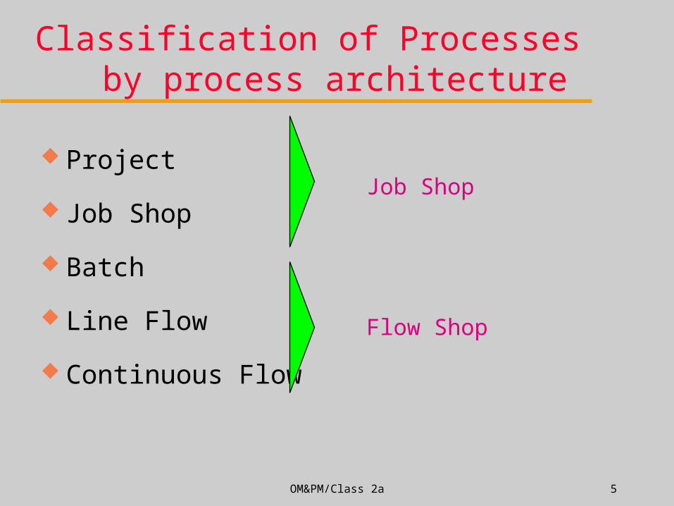
Classification of Processesby process architecture
Project
Job Shop
Batch
Line Flow
Continuous Flow
Job Shop
Flow Shop

OM&PM/Class 2a 6
Characteristics of Processes:Job Shop vs. Batch vs. Flow Shop
Type ofProcess
ProductVolume
SpecializedEquipment
ProductVariety
MachineSetup
Frequency
LaborSkills
VariableCost
Job Shop
Batch
Flow Shop

OM&PM/Class 2a 7
Matching Products and Processes withthe Product-Process Matrix
Capital Investment for bigchunk capacity,Technological Change,Vertical Integration
Product
ProcessJumbled Flow.Process segmentsloosely linked.
Disconnected LineFlow/Jumbled Flowbut a dominant flowexists.
JOB SHOP
(Commercial Printer)
BATCH
(Heavy Equipment)
LINE FLOWS
(Auto Assembly)
CONTINUOUS FLOW
(Oil Refinery)
Low volumeLow Standardization
One of a kind
Low volume
Many Products
Higher volume
Few Major Products
High volumeHigh StandardizationCommodity Products
Connected LineFlow (assembly line)
Continuous, automated,rigid line flow.Process segments tightlylinked.
Bidding, delivery,product design flexibility
Quality & Product Differentiation,output volume flexibility
Price
Scheduling,Materials Handling,Shifting Bottlenecks
Worker Motivation,Balance,Maintaining Flexibility
ManagerialChallenges
Opportunity
Costs
Out-of-pocket
Costs

OM&PM/Class 2a 8
Michigan Manufacturing Corp.:using the Product-Process Matrix
ProductProcess
Jumbled Flow.Process segments
loosely linked.
Job Shop
Disconnected LineFlow/Jumbled Flowbut a dominant flow
exists.
Batch
Low volumeLow Standardization
One of a kind
Low volume
Many Products
Higher volume
Few Major Products
High volumeHigh StandardizationCommodity Products
Connected LineFlow (assembly line)
Line Flow
Continuous, automated,rigid line flow.
Process segments tightlylinked.
Continuous Flow
1
10
100
1.0
10.0 100.0
(Designed Dollar) Volume per family
# ro
utes
(pr
oduc
t fa
mili
es)
Pontiac
LimaEssex
Saginaw
Sandusky
Tiffin
Fremont
Lebanon Maysville

OM&PM/Class 2a 9
Classification of Processes:by Positioning Strategy
Functional Focus:
Product Focus:
A B
C D
Product 1
Product 2
A D B
C B A
Product 1
Product 2
= resource pool (e.g., X-ray dept, billing)

OM&PM/Class 2a 10
Classification of Processes:by Customer Interface
Make to Stock
Make to Order

OM&PM/Class 2a 11
How can operations help a company compete?The changing sources of competitive advantage
Low Cost & Scale Economies (< 1960s)
– You can have any color you want as long as it is black
Focused Factories (mid 1960s)
Flexible Factories and Product variety (1970s)
– A car for every taste and purse.
Quality (1980s)
– Quality is free.
Time (late 1980s-1990s)
– We love your product but where is it?
– Don’t sell what you produce. produce what sells.
OM&PM/Class 2a 12
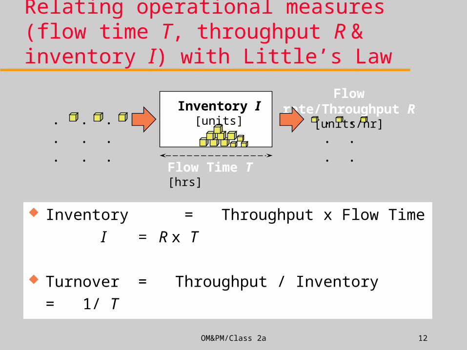
Relating operational measures (flow time T, throughput R & inventory I) with Little’s Law
Inventory = Throughput x Flow Time
I = R x T
Turnover = Throughput / Inventory
= 1/ T
Inventory I[units]
Flow rate/Throughput R
[units/hr]... ...... ......
Flow Time T [hrs]
OM&PM/Class 2a 13
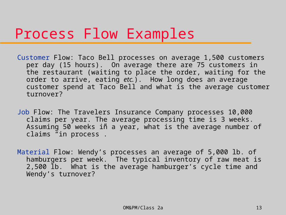
Process Flow Examples
Customer Flow: Taco Bell processes on average 1,500 customers per day (15 hours). On average there are 75 customers in the restaurant (waiting to place the order, waiting for the order to arrive, eating etc.). How long does an average customer spend at Taco Bell and what is the average customer turnover?
Job Flow: The Travelers Insurance Company processes 10,000 claims per year. The average processing time is 3 weeks. Assuming 50 weeks in a year, what is the average number of claims “in process”.
Material Flow: Wendy’s processes an average of 5,000 lb. of hamburgers per week. The typical inventory of raw meat is 2,500 lb. What is the average hamburger’s cycle time and Wendy’s turnover?

OM&PM/Class 2a 14
Process Flow Examples
Cash Flow: Motorola sells $300 million worth of cellular equipment per year. The average accounts receivable in the cellular group is $45 million. What is the average billing to collection process cycle time?
Question: A general manager at Baxter states that her inventory turns three times a year. She also states that everything that Baxter buys gets processed and leaves the docks within six weeks. Are these statements consistent?

CRU Computer Rentals
OM&PM/Class 2a 16
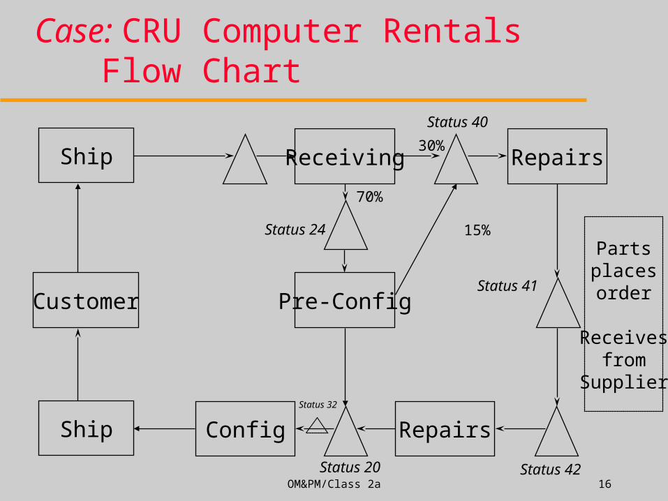
Case: CRU Computer RentalsFlow Chart
Customer
Receiving Repairs
Pre-Config
Partsplacesorder
Receivesfrom
Supplier
Repairs
Status 40
Status 24
Status 41
Status 42Status 20
Config
30%
70%
15%
ShipStatus 32
Ship

OM&PM/Class 2a 17
CRU Situation in 1996:Customer term = 8 wks, Demand = 1000 units/wk
Customer Receiving Status24
Status40
Parts Suppliers Status 41 Status 42 Status 20
Throughput(units/week)
1,000 1,000 700 300 +105 =405
405 405 405 405 1,000
Inventory(units)
8,000 500 1,500 1,000 500 405 500+405= 905
500 2,000
Flow Time(weeks)
8.0 0.5 2.14 2.47 1.23 1 2.23 1.23 2

OM&PM/Class 2a 18
CRU Situation in 1996:Financial Performance
Number of units on rent = 8,000 Total number of units = 14,405 Utilization = 0.56 (56%) Revenue rate = 8,000 x 30 = $240,000/wk Variable Cost rate = 25 x 1,000 (R) + 25 x 1,000 (S)
+ 4x700x.85 + 150 x 405 = $113,130/wk Contribution Margin = $126,870/wk Depreciation = 14,405 x ($1000/156wks) =
$92,340/wk– bottomline =
OM&PM/Class 2a 19
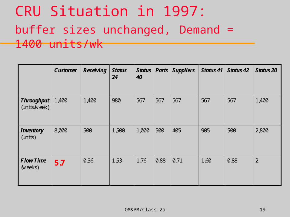
CRU Situation in 1997: buffer sizes unchanged, Demand = 1400 units/wk
Customer Receiving Status24
Status40
Parts Suppliers Status 41 Status 42 Status 20
Throughput(units/week)
1,400 1,400 980 567 567 567 567 567 1,400
Inventory(units)
8,000 500 1,500 1,000 500 405 905 500 2,800
Flow Time(weeks)
5.7 0.36 1.53 1.76 0.88 0.71 1.60 0.88 2
OM&PM/Class 2a 20
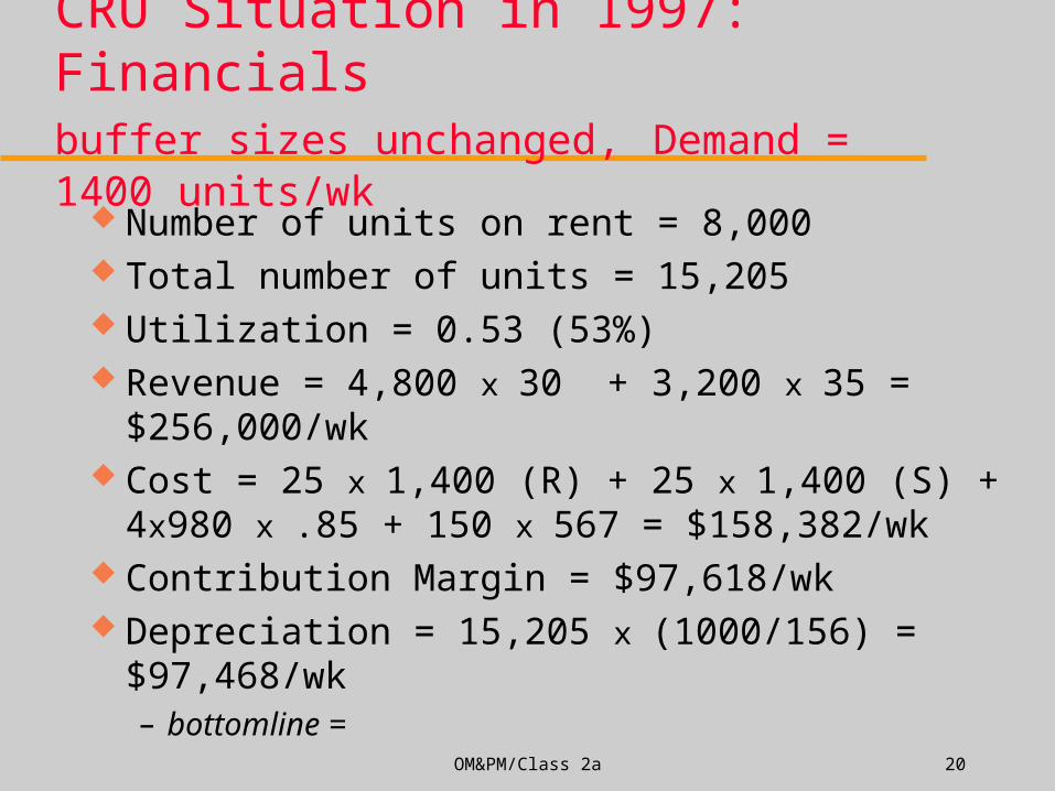
CRU Situation in 1997: Financialsbuffer sizes unchanged, Demand = 1400 units/wk
Number of units on rent = 8,000 Total number of units = 15,205 Utilization = 0.53 (53%) Revenue = 4,800 x 30 + 3,200 x 35 = $256,000/wk Cost = 25 x 1,400 (R) + 25 x 1,400 (S) + 4x980 x .85
+ 150 x 567 = $158,382/wk Contribution Margin = $97,618/wk Depreciation = 15,205 x (1000/156) = $97,468/wk
– bottomline =
OM&PM/Class 2a 21
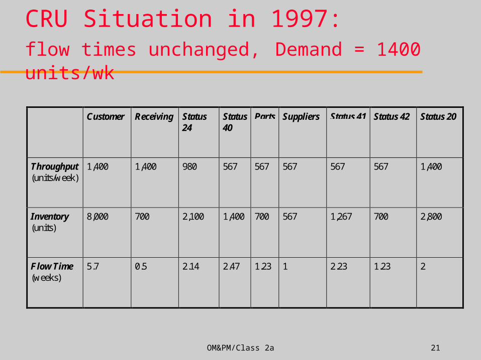
CRU Situation in 1997: flow times unchanged, Demand = 1400 units/wk
Customer Receiving Status24
Status40
Parts Suppliers Status 41 Status 42 Status 20
Throughput(units/week)
1,400 1,400 980 567 567 567 567 567 1,400
Inventory(units)
8,000 700 2,100 1,400 700 567 1,267 700 2,800
Flow Time(weeks)
5.7 0.5 2.14 2.47 1.23 1 2.23 1.23 2
OM&PM/Class 2a 22
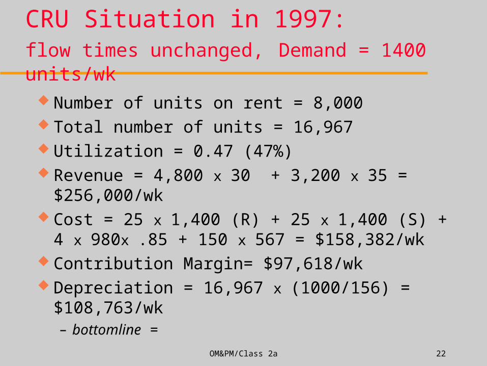
CRU Situation in 1997: flow times unchanged, Demand = 1400 units/wk
Number of units on rent = 8,000 Total number of units = 16,967 Utilization = 0.47 (47%) Revenue = 4,800 x 30 + 3,200 x 35 = $256,000/wk Cost = 25 x 1,400 (R) + 25 x 1,400 (S) + 4 x 980x .85
+ 150 x 567 = $158,382/wk Contribution Margin= $97,618/wk Depreciation = 16,967 x (1000/156) = $108,763/wk
– bottomline =
OM&PM/Class 2a 23
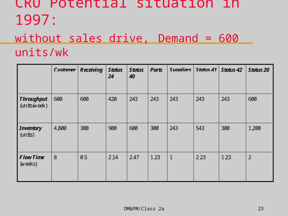
CRU Potential situation in 1997:without sales drive, Demand = 600 units/wk
Customer Receiving Status24
Status40
Parts Suppliers Status 41 Status 42 Status 20
Throughput(units/week)
600 600 420 243 243 243 243 243 600
Inventory(units)
4,800 300 900 600 300 243 543 300 1,200
Flow Time(weeks)
8 0.5 2.14 2.47 1.23 1 2.23 1.23 2

OM&PM/Class 2a 24
CRU Potential situation in 1997:without sales drive, Demand = 600 units/wk
Number of units on rent = 4,800 Total number of units = 8,643 Utilization = 0.56 (56%) Revenue = 4,800 x 30 = $144,000/wk Cost = 25 x 600 (R) + 25 x 600 (S) + 4x420x .85 +
150 x 243 = $67,878/wk Contribution Margin = $76,122/wk Depreciation = 8,643 x (1000/156) = $55,404/wk
– bottomline =

OM&PM/Class 2a 25
Lecture 2a Learning Objectives
Classification of processes– Match with strategy
Process Measures: time, inventory, and throughput What is an improvement?
– Link financial measures to operational ones
– Good operational measures are leading indicators of financial performance
Using Little’s law for process flow analysis