of Solids Experimental Mechanics of...
30
Experimental Mechanics of Solids CESAR A. SCIAMMARELLA FEDERICO M. SCIAMMARELLA
Transcript of of Solids Experimental Mechanics of...

Experimental Mechanicsof Solids
CESAR A. SCIAMMARELLA
FEDERICO M. SCIAMMARELLA
Experimental Mechanicsof SolidsCesar A. Sciammarella and Federico M. SciammarellaNorthern Illinois University, USA
SCIAMMARELLA
SCIAMMARELLA
Experimental M
echanicsof Solids
Experimental solid mechanics is the study of materials to determine their physical properties. This study might include performing a stress analysis or measuring the extent of displacement, shape, strain and stress which a material suffers under controlled conditions. In the last few years there have been remarkable developments in experimental techniques that measure shape, displacement and strains and these sorts of experiments are increasingly conducted using computational techniques.
Experimental Mechanics of Solids is a comprehensive introduction to the topics, technologies and methods of experimental mechanics of solids. It begins by establishing the fundamentals of continuum mechanics, explaining key areas such as the equations used, stresses and strains, and two and three dimensional problems. Having laid down the foundations of the topic, the book then moves on to look at specifi c techniques and technologies with emphasis on the most recent developments such as optics and image processing. Most of the current computational methods, as well as practical ones, are included to ensure that the book provides information essential to the reader in practical or research applications.
Key features:
• Presents widely used and accepted methodologies that are based on research and development work of the lead author
• Systematically works through the topics and theories of experimental mechanics including detailed treatments of the Moire, Speckle and holographic optical methods
• Includes illustrations and diagrams to illuminate the topic clearly for the reader
• Provides a comprehensive introduction to the topic, and also acts as a quick reference guide
• Accompanied by a website www.wiley.com/go/sciammarella hosting problems and solutions.
This comprehensive book forms an invaluable resource for graduate students and is also a point of reference for researchers and practitioners in structural and materials engineering.
Cover design: Jim Wilkie
Red box rules are for proof stage only. Delete before final printing.

P1: TIX/XYZ P2: ABCJWST117-fm JWST117-Sciammarella February 22, 2012 11:25 Printer Name: Yet to Come

P1: TIX/XYZ P2: ABCJWST117-fm JWST117-Sciammarella February 22, 2012 11:25 Printer Name: Yet to Come
EXPERIMENTALMECHANICS OF SOLIDS

P1: TIX/XYZ P2: ABCJWST117-fm JWST117-Sciammarella February 22, 2012 11:25 Printer Name: Yet to Come

P1: TIX/XYZ P2: ABCJWST117-fm JWST117-Sciammarella February 22, 2012 11:25 Printer Name: Yet to Come
EXPERIMENTALMECHANICS OF SOLIDS
Cesar A. SciammarellaResearch Professor, Mechanical Engineering, Northern Illinois University, DeKalb IL, USA
Federico M. SciammarellaAssistant Professor, Mechanical Engineering, Northern Illinois University, DeKalb IL, USA
A John Wiley & Sons, Ltd., Publication
P1: TIX/XYZ P2: ABCJWST117-fm JWST117-Sciammarella February 22, 2012 11:25 Printer Name: Yet to Come
This edition first published 2012© 2012, John Wiley & Sons, Ltd
Registered officeJohn Wiley & Sons Ltd, The Atrium, Southern Gate, Chichester, West Sussex, PO19 8SQ, United Kingdom
For details of our global editorial offices, for customer services and for information about how to apply forpermission to reuse the copyright material in this book please see our website at www.wiley.com.
The right of the author to be identified as the author of this work has been asserted in accordance with the Copyright,Designs and Patents Act 1988.
All rights reserved. No part of this publication may be reproduced, stored in a retrieval system, or transmitted, in anyform or by any means, electronic, mechanical, photocopying, recording or otherwise, except as permitted by the UKCopyright, Designs and Patents Act 1988, without the prior permission of the publisher.
Wiley also publishes its books in a variety of electronic formats. Some content that appears in print may not beavailable in electronic books.
Designations used by companies to distinguish their products are often claimed as trademarks. All brand names andproduct names used in this book are trade names, service marks, trademarks or registered trademarks of theirrespective owners. The publisher is not associated with any product or vendor mentioned in this book. Thispublication is designed to provide accurate and authoritative information in regard to the subject matter covered. It issold on the understanding that the publisher is not engaged in rendering professional services. If professional adviceor other expert assistance is required, the services of a competent professional should be sought.
MATLAB R© is a trademark of The MathWorks, Inc. and is used with permission. The MathWorks does not warrantthe accuracy of the text or exercises in this book. This book’s use or discussion of MATLAB R© software or relatedproducts does not constitute endorsement or sponsorship by The MathWorks of a particular pedagogical approach orparticular use of the MATLAB R© software.
Library of Congress Cataloging-in-Publication Data
Sciammarella, Cesar A.Experimental mechanics of solids / Cesar A. Sciammarella, Federico M. Sciammarella.
p. cm.Includes bibliographical references and index.ISBN 978-0-470-68953-0 (cloth : alk. paper)
1. Strength of materials. 2. Solids–Mechanical properties. 3. Structural analysis (Engineering)I. Sciammarella, F. M. (Federico M.) II. Title.
TA405.S3475 2012620.1′05–dc23
2011038404
A catalogue record for this book is available from the British Library.
ISBN: 978-0-470-68953-0
Typeset in 9/11pt Times by Aptara Inc., New Delhi, India

P1: TIX/XYZ P2: ABCJWST117-fm JWST117-Sciammarella February 22, 2012 11:25 Printer Name: Yet to Come
This book is dedicated to:Esther & Stephanie our loving wives and great supporters
Eduardo a great son and older brotherSasha and Lhasa – faithful companions

P1: TIX/XYZ P2: ABCJWST117-fm JWST117-Sciammarella February 22, 2012 11:25 Printer Name: Yet to Come
P1: TIX/XYZ P2: ABCJWST117-fm JWST117-Sciammarella February 22, 2012 11:25 Printer Name: Yet to Come
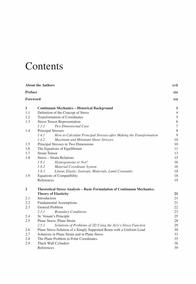
Contents
About the Authors xvii
Preface xix
Foreword xxi
1 Continuum Mechanics – Historical Background 11.1 Definition of the Concept of Stress 41.2 Transformation of Coordinates 51.3 Stress Tensor Representation 6
1.3.1 Two Dimensional Case 71.4 Principal Stresses 8
1.4.1 How to Calculate Principal Stresses after Making the Transformation 91.4.2 Maximum and Minimum Shear Stresses 10
1.5 Principal Stresses in Two Dimensions 101.6 The Equations of Equilibrium 111.7 Strain Tensor 131.8 Stress – Strain Relations 15
1.8.1 Homogeneous or Not? 161.8.2 Material Coordinate System 161.8.3 Linear, Elastic, Isotropic Materials. Lame Constants 18
1.9 Equations of Compatibility 18References 19
2 Theoretical Stress Analysis – Basic Formulation of Continuum Mechanics.Theory of Elasticity 21
2.1 Introduction 212.2 Fundamental Assumptions 212.3 General Problem 22
2.3.1 Boundary Conditions 232.4 St. Venant’s Principle 252.5 Plane Stress, Plane Strain 28
2.5.1 Solutions of Problems of 2D Using the Airy’s Stress Function 292.6 Plane Stress Solution of a Simply Supported Beam with a Uniform Load 302.7 Solutions in Plane Strain and in Plane Stress 332.8 The Plane Problem in Polar Coordinates 352.9 Thick Wall Cylinders 36
References 39

P1: TIX/XYZ P2: ABCJWST117-fm JWST117-Sciammarella February 22, 2012 11:25 Printer Name: Yet to Come
viii Contents
3 Strain Gages – Introduction to Electrical Strain Gages 413.1 Strain Measurements – Point Methods 413.2 Electrical Strain Gages 423.3 Basics of Electrical Strain Gages 43
3.3.1 Backing Material 433.3.2 Cements 443.3.3 Application of Gages onto Surfaces 45
3.4 Gage Factor 453.4.1 Derivation of Gage Factor 453.4.2 Alloys for Strain Gages 473.4.3 Semiconductor Strain Gages 48
3.5 Basic Characteristics of Electrical Strain Gages 483.5.1 Electrical Resistance 483.5.2 Temperature Effect 493.5.3 Corrections for Thermal Output 513.5.4 Adjusting Thermal Output for Gage Factor 53
3.6 Errors Due to the Transverse Sensitivity 543.6.1 Corrections Due to the Transversal Sensitivity 55
3.7 Errors Due to Misalignment of Strain Gages 583.8 Reinforcing Effect of the Gage 603.9 Effect of the Resistance to Ground 613.10 Linearity of the Gages. Hysteresis 633.11 Maximum Deformations 643.12 Stability in Time 643.13 Heat Generation and Dissipation 643.14 Effect of External Ambient Pressure 65
3.14.1 Additional Consideration Concerning the Effect of Pressure on Strain Gages 663.14.2 Additional Environment Effects to Consider 663.14.3 Electromagnetic Fields 67
3.15 Dynamic Effects 673.15.1 Transient Effects 673.15.2 Steady State Response. Fatigue Characteristics of Strain Gauges 69References 71
4 Strain Gages Instrumentation – The Wheatstone Bridge 754.1 Introduction 75
4.1.1 Derivation of the Wheatstone Equilibrium Condition 764.1.2 Full Bridge Arrangements in Some Simple Cases of Loadings 824.1.3 Linearity Errors of the Wheatstone Bridge with Constant Voltage 834.1.4 Temperature Compensation in the Bridge Circuit 874.1.5 Leadwire Resistance/Temperature Compensation 904.1.6 Shunt Calibration of Strain Gage Instrumentation 944.1.7 Series Resistance Null Balance 974.1.8 Available Commercial Instrumentation 984.1.9 Dynamic Measurements 1004.1.10 Potentiometer Circuit 1034.1.11 Operational Amplifiers 105References 109
P1: TIX/XYZ P2: ABCJWST117-fm JWST117-Sciammarella February 22, 2012 11:25 Printer Name: Yet to Come
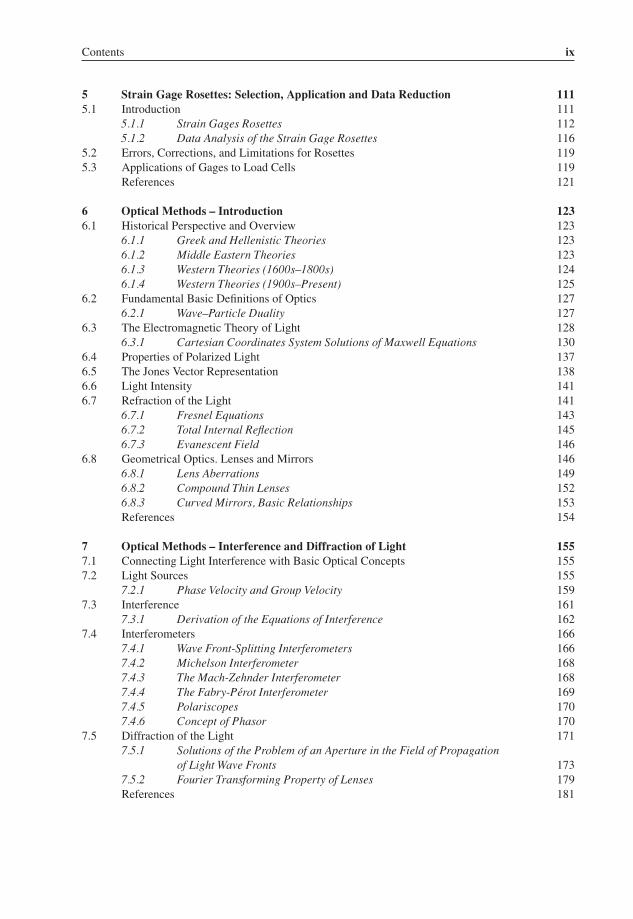
Contents ix
5 Strain Gage Rosettes: Selection, Application and Data Reduction 1115.1 Introduction 111
5.1.1 Strain Gages Rosettes 1125.1.2 Data Analysis of the Strain Gage Rosettes 116
5.2 Errors, Corrections, and Limitations for Rosettes 1195.3 Applications of Gages to Load Cells 119
References 121
6 Optical Methods – Introduction 1236.1 Historical Perspective and Overview 123
6.1.1 Greek and Hellenistic Theories 1236.1.2 Middle Eastern Theories 1236.1.3 Western Theories (1600s–1800s) 1246.1.4 Western Theories (1900s–Present) 125
6.2 Fundamental Basic Definitions of Optics 1276.2.1 Wave–Particle Duality 127
6.3 The Electromagnetic Theory of Light 1286.3.1 Cartesian Coordinates System Solutions of Maxwell Equations 130
6.4 Properties of Polarized Light 1376.5 The Jones Vector Representation 1386.6 Light Intensity 1416.7 Refraction of the Light 141
6.7.1 Fresnel Equations 1436.7.2 Total Internal Reflection 1456.7.3 Evanescent Field 146
6.8 Geometrical Optics. Lenses and Mirrors 1466.8.1 Lens Aberrations 1496.8.2 Compound Thin Lenses 1526.8.3 Curved Mirrors, Basic Relationships 153References 154
7 Optical Methods – Interference and Diffraction of Light 1557.1 Connecting Light Interference with Basic Optical Concepts 1557.2 Light Sources 155
7.2.1 Phase Velocity and Group Velocity 1597.3 Interference 161
7.3.1 Derivation of the Equations of Interference 1627.4 Interferometers 166
7.4.1 Wave Front-Splitting Interferometers 1667.4.2 Michelson Interferometer 1687.4.3 The Mach-Zehnder Interferometer 1687.4.4 The Fabry-Perot Interferometer 1697.4.5 Polariscopes 1707.4.6 Concept of Phasor 170
7.5 Diffraction of the Light 1717.5.1 Solutions of the Problem of an Aperture in the Field of Propagation
of Light Wave Fronts 1737.5.2 Fourier Transforming Property of Lenses 179References 181

P1: TIX/XYZ P2: ABCJWST117-fm JWST117-Sciammarella February 22, 2012 11:25 Printer Name: Yet to Come
x Contents
8 Optical Methods – Fourier Transform 1838.1 Introduction 1838.2 Simple Properties 185
8.2.1 Linearity 1858.2.2 Frequency Shifting 1858.2.3 Space Shifting 1858.2.4 Space Differentiation 1868.2.5 Correlation and Convolution 1868.2.6 Autocorrelation Function 1878.2.7 The Parseval’s Theorem 187
8.3 Transition to Two Dimensions 1878.4 Special Functions 188
8.4.1 Dirac Delta 1888.4.2 Comb Function 1898.4.3 Rectangle Function 1908.4.4 The Signum Function 1918.4.5 Circle Function 191
8.5 Applications to Diffraction Problems 1918.5.1 Rectangular Aperture 1928.5.2 Circular Aperture 193
8.6 Diffraction Patterns of Gratings 1938.7 Angular Spectrum 1958.8 Utilization of the FT in the Analysis of Diffraction Gratings 199
8.8.1 An Approximated Method to Describe the Diffraction Pattern of Gratings 202References 205
9 Optical Methods – Computer Vision 2079.1 Introduction 2079.2 Study of Lens Systems 2089.3 Lens System, Coordinate Axis and Basic Layout 2109.4 Diffraction Effect on Images 211
9.4.1 Examples of Pupils 2149.5 Analysis of the Derived Pupil Equations for Coherent Illumination 2169.6 Imaging with Incoherent Illumination 217
9.6.1 Coherent and Non Coherent Illumination. Effect on the Image 2219.6.2 Criteria for the Selection of Lenses 2269.6.3 Standard Nomenclatures 227
9.7 Digital Cameras 2309.7.1 CCDs and CMOSs 2309.7.2 Monochrome vs. Color Cameras 2339.7.3 Basic Notions in the Image Acquisition Process 2359.7.4 Exposure Time of a Sensor. Relationship to the Object Intensity 2359.7.5 Sensor Size 239
9.8 Illumination Systems 2429.8.1 Radiometry 2429.8.2 Interaction of Light with Matter and Directional Properties 2449.8.3 Illumination Techniques 245
9.9 Imaging Processing Systems 2459.9.1 Frame Grabbers 246
P1: TIX/XYZ P2: ABCJWST117-fm JWST117-Sciammarella February 22, 2012 11:25 Printer Name: Yet to Come
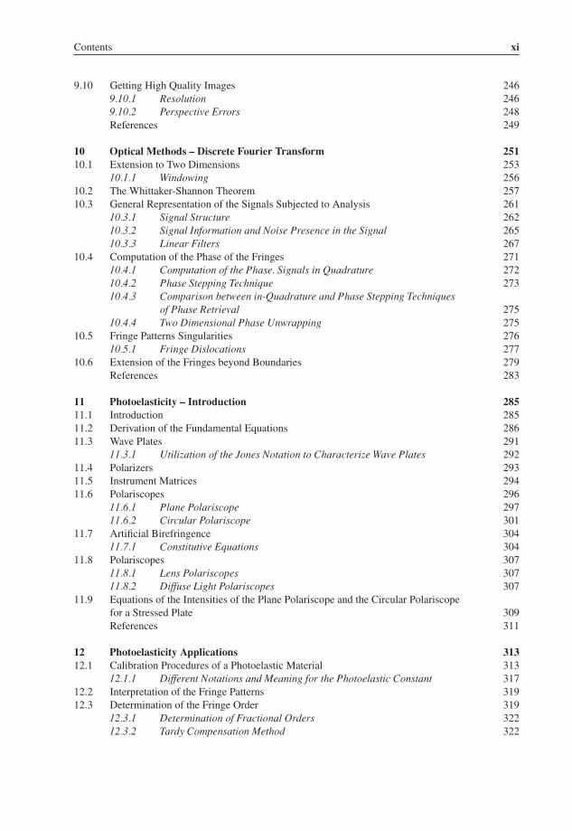
Contents xi
9.10 Getting High Quality Images 2469.10.1 Resolution 2469.10.2 Perspective Errors 248References 249
10 Optical Methods – Discrete Fourier Transform 25110.1 Extension to Two Dimensions 253
10.1.1 Windowing 25610.2 The Whittaker-Shannon Theorem 25710.3 General Representation of the Signals Subjected to Analysis 261
10.3.1 Signal Structure 26210.3.2 Signal Information and Noise Presence in the Signal 26510.3.3 Linear Filters 267
10.4 Computation of the Phase of the Fringes 27110.4.1 Computation of the Phase. Signals in Quadrature 27210.4.2 Phase Stepping Technique 27310.4.3 Comparison between in-Quadrature and Phase Stepping Techniques
of Phase Retrieval 27510.4.4 Two Dimensional Phase Unwrapping 275
10.5 Fringe Patterns Singularities 27610.5.1 Fringe Dislocations 277
10.6 Extension of the Fringes beyond Boundaries 279References 283
11 Photoelasticity – Introduction 28511.1 Introduction 28511.2 Derivation of the Fundamental Equations 28611.3 Wave Plates 291
11.3.1 Utilization of the Jones Notation to Characterize Wave Plates 29211.4 Polarizers 29311.5 Instrument Matrices 29411.6 Polariscopes 296
11.6.1 Plane Polariscope 29711.6.2 Circular Polariscope 301
11.7 Artificial Birefringence 30411.7.1 Constitutive Equations 304
11.8 Polariscopes 30711.8.1 Lens Polariscopes 30711.8.2 Diffuse Light Polariscopes 307
11.9 Equations of the Intensities of the Plane Polariscope and the Circular Polariscopefor a Stressed Plate 309References 311
12 Photoelasticity Applications 31312.1 Calibration Procedures of a Photoelastic Material 313
12.1.1 Different Notations and Meaning for the Photoelastic Constant 31712.2 Interpretation of the Fringe Patterns 31912.3 Determination of the Fringe Order 319
12.3.1 Determination of Fractional Orders 32212.3.2 Tardy Compensation Method 322
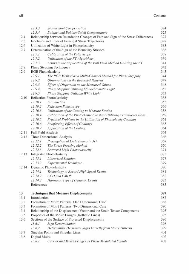
P1: TIX/XYZ P2: ABCJWST117-fm JWST117-Sciammarella February 22, 2012 11:25 Printer Name: Yet to Come
xii Contents
12.3.3 Seanarmont Compensation 32412.3.4 Babinet and Babinet-Soleil Compensators 325
12.4 Relationship between Retardation Changes of Path and Sign of the Stress Differences 32712.5 Isoclinics and Lines of Principal Stress Trajectories 32812.6 Utilization of White Light in Photoelasticity 33312.7 Determination of the Sign of the Boundary Stresses 338
12.7.1 Calibration of the Polariscope 33812.7.2 Utilization of the FT Algorithms 33912.7.3 Errors in the Application of the Full Field Method Utilizing the FT 341
12.8 Phase Stepping Techniques 34212.9 RGB Photoelasticity 343
12.9.1 The RGB Method as a Multi-Channel Method for Phase Stepping 34412.9.2 Observations on the Recorded Patterns 34712.9.3 Effect of Dispersion on the Measured Values 34812.9.4 Phase Stepping Utilizing Monochromatic Light 35212.9.5 Phase Stepping Utilizing White Light 353
12.10 Reflection Photoelasticity 35512.10.1 Introduction 35512.10.2 Reflection Polariscope 35612.10.3 Utilization of the Coating to Measure Strains 35812.10.4 Calibration of the Photoelastic Constant Utilizing a Cantilever Beam 35912.10.5 Practical Problems in the Utilization of Photoelastic Coatings 36112.10.6 Reinforcing Effects of Coatings 36312.10.7 Application of the Coating 364
12.11 Full Field Analysis 36412.12 Three Dimensional Analysis 366
12.12.1 Propagation of Light Beams in 3D 36712.12.2 The Stress Freezing Method 37012.12.3 Scattered Light Photoelasticity 371
12.13 Integrated Photoelasticity 37512.13.1 Linearized Solution 37712.13.2 Experimental Technique 379
12.14 Dynamic Photoelasticity 38012.14.1 Technology to Record High Speed Events 38112.14.2 CCD and CMOS 38212.14.3 Harmonic Type of Dynamic Events 383References 383
13 Techniques that Measure Displacements 38713.1 Introduction 38713.2 Formation of Moire Patterns. One Dimensional Case 38813.3 Formation of Moire Patterns. Two Dimensional Case 39013.4 Relationship of the Displacement Vector and the Strain Tensor Components 39313.5 Properties of the Moire Fringes (Isothetic Lines) 39513.6 Sections of the Surface of Projected Displacements 396
13.6.1 Sign Determination 39813.6.2 Determining Derivative Signs Directly from Moire Patterns 399
13.7 Singular Points and Singular Lines 40113.8 Digital Moire 402
13.8.1 Carrier and Moire Fringes as Phase Modulated Signals 402
P1: TIX/XYZ P2: ABCJWST117-fm JWST117-Sciammarella February 22, 2012 11:25 Printer Name: Yet to Come
Contents xiii
13.8.2 Generalization to Two Dimensions of the Equations Relating Moire Patternsto Displacements 405
13.8.3 Limits to the Continuous Optical Law 40813.9 Equipment Required to Apply the Moire Method for Displacement and Strain
Determination Utilizing Incoherent Illumination 41213.9.1 Printing Gratings on Model Surfaces 41313.9.2 Optical Arrangements to Generate Incoherent Light Moire Patterns 41413.9.3 Effect of the Camera in the Captured Image, Gap Effect 41513.9.4 Application of Moire to 2D Static Problems Using Incoherent Illumination 417
13.10 Strain Analysis at the Sub-Micrometer Scale 41913.10.1 Fundamental Parameters and Optical Set Up 41913.10.2 Results of Measurements Made at Sub-Micron Level 421
13.11 Three Dimensional Moire 42413.11.1 Model Construction. Observation Set Up 424
13.12 Dynamic Moire 426References 432
14 Moire Method. Coherent Ilumination 43514.1 Introduction 43514.2 Moire Interferometry 43514.3 Optical Developments to Obtain Displacement, Contours and Strain Information 439
14.3.1 Fringe Pattern Separations and Fringe Multiplication 44014.3.2 Pattern Interpolation 44114.3.3 Differentiation of the Patterns 442
14.4 Determination of All the Components of the Displacement Vector 3-DInterferometric Moire 44614.4.1 Determination of the Components u and v 44614.4.2 Determination of the w Component 44714.4.3 Development of a Moire Interferometer Removing the FT Part of the
Original Interferometer 45014.5 Application of Moire Interferometry to High Temperature Fracture Analysis 451
References 456
15 Shadow Moire & Projection Moire – The Basic Relationships 45915.1 Introduction 45915.2 Basic Equation of Shadow Moire 46015.3 Basic Differential Geometry Properties of Surfaces 46115.4 Connection between Differential Geometry and Moire 46315.5 Projective Geometry and Projection Moire 467
15.5.1 The Pinhole Camera Model 46715.6 Epipolar Model of the Two Projectors and One Camera System 46915.7 Approaches to Extend the Moire Method to More General Conditions of Projection
and Observation 47115.7.1 Pitch of a Grating Projected from a Point Source on the Reference Plane 47515.7.2 Removal of the Effect of the Projection from a Point Source 47715.7.3 General Formulation of the Contouring Problem 47815.7.4 Merging of the Observed Patterns to a Common Coordinate System 481
15.8 Summary of the Chapter 482References 482
P1: TIX/XYZ P2: ABCJWST117-fm JWST117-Sciammarella February 22, 2012 11:25 Printer Name: Yet to Come
xiv Contents
16 Moire Contouring Applications 48516.1 Introduction 48516.2 Basic Principles of Optical Contouring Measuring Devices 48616.3 Contouring Methods that Utilize Projected Carriers 48616.4 Parallax Determination in an Area 48916.5 Mathematical Modeling of the Parallax Determination in an Area 490
16.5.1 Utilization of Several Cameras and Projectors 49216.6 Limitations of the Contouring Model 49216.7 Applications of the Contouring Methods 494
16.7.1 Application of 1 Camera and 1 Projector Systems: Contouring Large SlopeSurfaces 495
16.7.2 Application of 1 Camera and 1 Projector Systems: DeformationMeasurements of Flat Surfaces 501
16.8 Double Projector System with Slope and Depth-of-Focus Corrections 50616.8.1 Deflection Measurement of Large-Size Composite Panel 50816.8.2 Contouring of Selective Laser Sintering Sample 51216.8.3 Determination of the Geometric Primitives for the Stereolithographic Sample 514
16.9 Sensitivity Limits for Contouring Methods 518References 520
17 Reflection Moire 52317.1 Introduction 52317.2 Incoherent Illumination. Derivation of the Fundamental Relationship 523
17.2.1 Optical Set-Ups to Observe Slope Fringes in Incoherent Illumination 52517.3 Interferometric Reflection Moire 526
17.3.1 Derivation of the Equation of the Interferometric Reflection Moire Fringes 52717.4 Analysis of the Sensitivity that can be Achieved with the Described Setups 53017.5 Determination of the Deflection of Surfaces Using Reflection Moire 53117.6 Applications of the Reflection Moire Method 532
17.6.1 Measurement of Residual Stresses in Electronic Chips 53417.6.2 Examples. Finished Wafer 53417.6.3 Curvatures of the Chips 536
17.7 Reflection Moire Application – Analysis of a Shell 539References 545
18 Speckle Patterns and Their Properties 54718.1 Introduction 54718.2 First Order Statistics 550
18.2.1 Additional Statistical Results 55318.2.2 Addition in Intensity of a Uniform Background 55318.2.3 Second Order Statistics. Objective Speckle Field 55418.2.4 Extension of the Results Obtained in the Objective Speckle Field to the
Subjective Speckle Field 55618.3 Three Dimensional Structure of Speckle Patterns 55818.4 Sensor Effect on Speckle Statistics 56018.5 Utilization of Speckles to Measure Displacements. Speckle Interferometry 56218.6 Decorrelation Phenomena 56418.7 Model for the Formation of the Interference Fringes 56718.8 Integrated Regime. Metaspeckle 56918.9 Sensitivity Vector 572
P1: TIX/XYZ P2: ABCJWST117-fm JWST117-Sciammarella February 22, 2012 11:25 Printer Name: Yet to Come
Contents xv
18.10 Speckle Techniques Set-Ups 57318.10.1 The Double Beam Interferometer 57318.10.2 Out-of-Plane Component 576
18.11 Out-of-Plane Interferometer 57618.12 Shear Interferometry (Shearography) 57718.13 Contouring Interferometer 57818.14 Double Viewing. Duffy Double Aperture Method 579
References 581
19 Speckle 2 58319.1 Speckle Photography 58319.2 Point-Wise Observation of the Speckle Field 58419.3 Global View 58519.4 Different Set-Ups for Speckle Photography 58919.5 Applications of Speckle Interferometry 590
19.5.1 Data Recording and Processing 59019.5.2 Extension of the Range of Applied Loading 592
19.6 High Temperature Strain Measurement 59319.7 Four Beam Interferometer Sensitive to in Plane Displacements 597
19.7.1 Interfacial Deformation between Particles and Matrix in ParticleReinforced Composites 598
19.7.2 Stress Analysis of Weldments and Verification of Finite ElementMethod Results 601
19.7.3 Measurement of Mechanical Properties in Specimens of MicronSize Dimensions 604
References 606
20 Digital Image Correlation (DIC) 60720.1 Introduction 60720.2 Process to Obtain the Displacement Information 60820.3 Basic Formulation of the Problem 61020.4 Introduction of Smoothing Functions to Solve the Optimization Problem 613
20.4.1 Application of the Bicubic Spline Method to the Optimization Problemin DIC 615
20.5 Determination of the Components of the Displacement Vector 61820.6 Important Factors that Influence the Packages of DIC 61920.7 Evaluation of the DIC Method 62120.8 Double Viewing DIC. Stereo Vision 627
References 628
21 Holographic Interferometry 63121.1 Holography 63121.2 Basic Elements of the Holographic Process 632
21.2.1 Recording a Hologram 63221.2.2 Reconstruction of the Hologram 633
21.3 Properties of Holograms 63421.4 Set up to Record Holograms 636
21.4.1 Recording Media 64021.4.2 Speckles Presence in Hologram Recordings 640
P1: TIX/XYZ P2: ABCJWST117-fm JWST117-Sciammarella February 22, 2012 11:25 Printer Name: Yet to Come
xvi Contents
21.5 Holographic Interferometry 64121.5.1 Analysis of the Formation of Holographic Fringes 642
21.6 Derivation of the Equation of the Sensitivity Vector 64421.7 Measuring Displacements 64621.8 Holographic Moire 65121.9 Lens Holography 658
21.9.1 Fringe Spacing of the Fictitious Displacement, Fringes and FringeLocalization 660
21.10 Holographic Moire. Real Time Observation 66121.11 Displacement Analysis of Curved Surfaces 665
21.11.1 Analysis of a Pipe under Internal Pressure 66821.12 Holographic Contouring 669
21.12.1 Factors Influencing the Separation of Fringes 67121.13 Measurement of Displacements in 3D of Transparent Bodies 67521.14 Fiber Optics Version of the Holographic Moire System 675
References 677
22 Digital and Dynamic Holography 68122.1 Digital Holography 681
22.1.1 Digital Holographic Interferometry 68422.2 Determination of Strains from 3D Holographic Moire Interferograms 68522.3 Introduction to Dynamic Holographic Interferometry 689
22.3.1 Vibration Phenomena in Holographic Interferometry 68922.3.2 Sinusoidal Vibrations 69022.3.3 Holoraphic Interferometry Fringes 69222.3.4 Stroboscopic Illumination 692
22.4 Vibration Analysis 69322.5 Experimental Set up for Time Average Holography 695
22.5.1 Experimental Procedure to Obtain Resonant Modes of a Turbine Blade 69622.5.2 Experimental Set up to Record Dynamical Holograms with Stroboscopic
Illumination 69622.5.3 Holographic Set up to Obtain Strain and Stresses of a Vibrating Blade 69722.5.4 Vibration Modes and Stress Analysis of the SRB-SPU Turbine of the Space
Shuttle 69722.6 Investigation on Fracture Behavior of Turbine Blades Under Self-Exciting Modes 700
22.6.1 Experimental Technique for Vibration Analysis 70222.7 Dynamic Holographic Interferometry. Impact Analysis. Wave Propagation 708
22.7.1 Lasers Utilized in Dynamic Holographic Interferometry 70922.7.2 Applications of Pulsed Holographic Interferometry 709
22.8 Applications of Dynamic Holographic Interferometry 71222.8.1 Application to Non Destructive Evaluation 712References 721
Index 723

P1: TIX/XYZ P2: ABCJWST117-ABOUT-AUTHOR JWST117-Sciammarella December 26, 2011 9:40 Printer Name: Yet to Come
About the Authors
Cesar A. Sciammarella was Director of the world renowned Experimental Mechanics Laboratory at theIllinois Institute of Technology for more than 30 years. Over that time he made pioneering developmentsin applying moire, holography, and speckle interferometry methodologies as an experimental tool tosolve industrial problems around the world. He recently completed a five year project funded by theItalian government to help the Politecnico of Bari develop its experimental mechanics lab and increaseits future talent. Currently he is Research Professor at Northern Illinois University where he is workingon various industrial projects involving optical contouring and experimental mechanics down at thenanometric level. This effort has taken him beyond the Rayleigh limit that traditionally was consideredas the maximum resolution that could be obtained in optics in far field observations. His recent workhas yielded measurements in the far field of nanocrystals and nanospheres with accuracies on the orderof ±3.3 nm. His recent discoveries will no doubt lead this field as he has done in the past. He hasbeen an active member in the Society of Experimental Mechanics where he has received almost everyhonor possible.
Federico M. Sciammarella joined the College of Engineering and Engineering Technology at NorthernIllinois University in 2007 and is an assistant professor in the Mechanical Engineering Department. Histwo research areas are laser materials processing and experimental mechanics. One of several projectsinvolves laser assisted machining (LAM) of ceramics through NIU’s Rapid Optimization of CommercialKnowledge (ROCK) Project. The ROCK project enhances the capabilities of small companies by workingthrough supply chains and with experts to improve their productivities and process. He has now spent sometime using a novel optical method developed with his father and colleague Dr. Lamberti, Advanced DigitalMoire Contouring to measure surface roughness of the ceramic bars after the LAM process. Throughits mission, the ROCK project, working with local companies, strive to develop niche technologies thatwill directly benefit the U.S. and by providing higher quality parts at reduced costs, improving supplylogistics, and creating new manufacturing tools and methods that are critical to the continued growth ofthis nation.

P1: TIX/XYZ P2: ABCJWST117-ABOUT-AUTHOR JWST117-Sciammarella December 26, 2011 9:40 Printer Name: Yet to Come
P1: TIX/XYZ P2: ABCJWST117-PRE JWST117-Sciammarella December 26, 2011 9:41 Printer Name: Yet to Come
Preface
The aim of this book, Experimental Mechanics of Solids, is to provide a comprehensive and in depth lookat the various approaches possible to analyze systems and materials via experimental mechanics. Thisfield has grown mostly through ideas, chance and pure intuition. This field is now mature enough that acomprehensive analysis on the nature of material properties is possible. Often we do things without toomuch thought and experimental mechanics is no exception.
The approach of this book is to break down each chapter into specific categories and provide somehistorical context so that the reader can understand how we have reached a certain level in the respectivefields. The first two chapters provide some insight into the fundamental issues with regards to continuummechanics and stress analysis that must be clear to the reader so that they may then make the appropriatedecisions when performing field measurements. The next three chapters deal with the use and applicationof strain gages. There has been a lot of work done in this field so the aim was to provide some basic andpractical information for the reader to be able to make sound choices with regards to a selection of gageand understanding the conditions for measurements. The remaining chapters deal with optical methods.Here for the first time ever the reader will see the unifying nature behind all these methods and shouldwalk away with a more complete understanding of the various optical techniques. Most importantly, allthe various examples that we have done over our careers are shared so that the reader can understand theadvantages of one method over another in a given application.
Ultimately this book should serve as both a learning tool and a resource for industry when faced withdifficult problems that only experimental mechanics can help solve. It is our hope that the students whoread this book will understand what it takes to perform research in this field and provide inspiration forthe future generations of experimentalists.
Our thanks go to Kristina Young M.S. who kindly rendered our illustrations.

P1: TIX/XYZ P2: ABCJWST117-PRE JWST117-Sciammarella December 26, 2011 9:41 Printer Name: Yet to Come

P1: TIX/XYZ P2: ABCJWST117-FWD JWST117-Sciammarella February 22, 2012 11:29 Printer Name: Yet to Come
Foreword
It is a great honor for me to write the foreword of Experimental Mechanics of Solids authored byProf. Cesar A. Sciammarella and Dr. Federico M. Sciammarella. I have been involved with the authorsfor the past 10 years. Professor C.A. Sciammarella has taught me optics and made me familiar withthe use of optics in that wonderful field called Experimental Solid Mechanics. Dr. F.M. Sciammarella,my friend, was a PhD student when I visited Prof. C.A. Sciammarella’s lab at the Illinois Institute ofTechnology. We took the class on Experimental Solid Mechanics taught by Prof. C.A. Sciammarella.Since then Fred and I collaborated on many pioneering studies carried out by the Professor.
I always asked Prof. Sciammarella to write a book with the purpose to disclose his enormous knowl-edge to young “fellows” who are interested in Experimental Solid Mechanics. In his five years at thePolitecnico in Bari, the Professor was very busy carrying out frontier research and organizing interna-tional conferences that brought world renowned scientists to Bari. In spite of all of this hard work, Prof.Sciammarella found the time for conceiving the general organization of his book. In October 2008, whenProf. Sciammarella moved back to US we promised to continue working together. I am glad to say thatProf. Sciammarella, Dr. Sciammarella and myself still work together and will work together in the future,always investigating new exciting topics.
I have seen this book being developed day by day, chapter by chapter. Prof. Sciammarella and Dr.Sciammarella have shown me several chapters of their work. I remember the discussions we had inChicago. There is no doubt that the quality of the book is outstanding. Apart from the technical contentthat is excellent in view of the high scientific reputation of the two authors, what has impressed me atthe first reading is the clarity of the presentation which has plenty of useful examples. At the secondreading, one realizes that the clarity is the obvious result of a total knowledge of the subject presented inthe book. I now teach experimental mechanics and I am eager to suggest this new book to my students.
Thank you very much Professor and Fred for having given this book to us!
Dr. Luciano LambertiAssociate Professor
Dipartimento di Ingegneria Meccanica e GestionalePolitecnico di Bari
BARI, ITALY

P1: TIX/XYZ P2: ABCJWST117-FWD JWST117-Sciammarella February 22, 2012 11:29 Printer Name: Yet to Come

P1: SFN/XYZ P2: ABCJWST117-c01 JWST117-Sciammarella February 8, 2012 23:39 Printer Name: Yet to Come
1Continuum Mechanics – HistoricalBackground
The fundamental problem that faces a structural engineer, civil, mechanical or aeronautical is to makeefficient use of the materials at their disposal to create shapes that will perform a certain function withminimum cost and high reliability whenever possible. There are two basic aspects of this process selectionof materials, and then selection of shape. Material scientists, on the basis of the demand generated byapplications, devote their efforts to creating the best possible materials for a given application. It is up tothe designer of the structure or mechanical component to make the best use of these materials by selectingshapes that will simultaneously provide the transfer of forces acting on the structure or component inan efficient, safe and economical fashion. Today, a designer has a variety of tools to achieve thesebasic goals.
These tools have evolved historically through a heritage that can be traced back to the great buildersof structures in 2700 BC Egypt, Greece and Rome, to the builders of cathedrals in the Middle Ages.Throughout the ancient and medieval period structural design was in the hands of master builders,helped by artisan masons and carpenters. During this period there is no evidence that structural theoriesexisted. The design process was based on empirical evidence, founded many times in trial and errorprocedures done at different scales. The Romans achieved great advances in structural engineering,building structures that are still standing today, like the Pantheon, a masonry semi-spherical vault witha bronze ring to take care of tension stresses in the right place. It took many centuries to arrive at thebeginning of a scientific approach to structures. It was the universal genius of the Renaissance LeonardoDa Vinci (1452–1519) one of the first designers that gives us evidence that scientific observations andrigorous analysis formed the basis of his designs. He was also an experimental mechanics pioneer andmany of his designs were based on extensive materials testing.
The text that follows will introduce the names of the most outstanding contributors to some of the basicideas of the mechanics of the continuum that we are going to review in this chapter. The next chapterprovides background on those who contributed further in the nineteenth century and early twentieth. Inthe twentieth century many of the basic ideas were reformulated in a more rigorous and comprehensivemathematical framework. At the same time basic principles were developed to formulate solid mechanicsproblems in terms of approximate solutions through numerical computation: Finite Element, BoundaryElement, Finite Differences.
The birth of the scientific approach to the design of structures can be traced back to Galileo Galilei.In 1638 Galileo published a manuscript entitled Dialogues Relating to Two New Sciences. This bookcan be considered as the precursor to the discipline Strength of Materials. It includes the first attempt
Experimental Mechanics of Solids, First Edition. Cesar A. Sciammarella and Federico M. Sciammarella.© 2012 John Wiley & Sons, Ltd. Published 2012 by John Wiley & Sons, Ltd.
1
P1: SFN/XYZ P2: ABCJWST117-c01 JWST117-Sciammarella February 8, 2012 23:39 Printer Name: Yet to Come
2 Experimental Mechanics of Solids
to develop the theory of beams by analyzing the behavior of a cantilever beam. A close successor ofGalileo was Robert Hook, curator of experiments at the Royal Society and professor of Geometry atGresham College, Oxford. In 1676, he introduced his famous Hooke’s law that provided the first scientificunderstanding of elasticity in materials.
At this point it is necessary to mention the contribution of Sir Isaac Newton, with the first systematicapproach to the science of Mechanics with the publication in 1687 of Philosophiae Naturalis PrincipiaMathematica. There is another important contribution of Newton and Gottfried Leibniz that helpedin the development of structural engineering; they established the basis of Calculus, a fundamentalmathematical tool in structural analysis.
From the eighteenth century, we must recall Leonard Euler, the mathematician who developed manyof the tools that are used today in structural analysis. He, together with Bernoulli, developed the funda-mental beam equation around 1750 by introducing the Euler-Bernoulli postulate of the plane sectionswhich remain plane after deformation. Another important contribution of Euler was his developmentsconcerning the phenomenon of buckling.
From the nineteenth century we recognize Thomas Young, English physicist and Foreign Secretary ofthe Royal Institute. Young introduced the concept of elastic modulus, the Young’s modulus, denoted asE, in 1807. The complete formulation of the basis of the theory of elasticity was done by Simon-DenisPoisson who introduced the concept of what is called today Poisson’s ratio.
Ausgustin-Louis Cauchy (1789–1857) the French mathematician, besides being an outstanding con-tribution to mathematics was one of the early creators of the field of what we call continuum mechanics,both through the introduction of the concept of stress tensor as well his extensive work on the theory ofdeformation of the continuum.
Claude-Louis Navier (1785–1836), a French engineer, professor of the Ecole de Ponts et Chaussees inParis, is considered to be the founder of structural analysis by developing many of the equations requiredfor the solution of structural problems and applying them to the construction of bridges.
Another contributor to the basic equations of the continuum is Gabriel Lame (1795–1870) Frenchmathematician, professor of physics at L’Ecole Polytechnique and professor of probability at the Sor-bonne and member of the French Academy. He made significant contributions to the elasticity theory(the Lame constants and Lame equations). He was one of the first authors to publish a book on the theoryof elasticity. In 1852 he published Lecons sur la theorie mathematique de l’elasticite des corps solides.Another outstanding contributor to the foundations of the mechanics of solids is the French engineerand mathematician Adhemar-Jean- Claude Barre de Saint Venant (1797–1880). His major contributionswere in the field of torsion and the bending of bars and the introduction of his principle that is keyto the formulation of the solutions in the continuum. The original statement was published in Frenchby Saint-Venant in 1852. The statement concerning his principle is to be found in Memoires sur latorsion des prismes. The Saint-Venant’s principle has made it possible to solve elasticity problems withcomplicated stress distributions, by transforming them into problems that are easier to solve.
G. B. Airy (1801–1892) mathematician and professor of Astronomy at Cambridge, introduced in 1862the concept of stress function. The idea of stress function was applied by Lame in his work on thickwalled vessels, by Boussineq in his work of contact stresses and by Charles Edward English, professorat the Department of Engineering at Cambridge University who applied the idea of stress functionsto the solution of problems of stress concentration (1913). August Edward Hough Love (1863–1940),English Mathematician Professor of Natural Philosophy at Oxford author of many papers on the field ofElasticity, author of, A treatise in the Mathematical Theory of Elasticity, first published in 1892.
Tulio Levi-Civita (1871–1941), professor of Rational Mechanics at the University of Padova. He wasone of the outstanding mathematicians of the 19th century. He introduced the idea of tensors and tensorcalculus that played a fundamental role in the field of mechanics of solids and in the Theory of Relativity.The contributors to the mechanics of solids includes the names of many outstanding mathematiciansand physicists of the nineteenth century: James Clerk Maxwell, H. Herzt, Eugenio Beltrami, John HenriMitchell, Carlo Alberto Castigliano, Luigi Federico Menabrea.
P1: SFN/XYZ P2: ABCJWST117-c01 JWST117-Sciammarella February 8, 2012 23:39 Printer Name: Yet to Come
Continuum Mechanics – Historical Background 3
Let us start with a basic approach to see how these different schools of thought are utilized. Hereis the scenario: Given a certain body subjected to given loads and given form of support what arethe stresses? In strength of materials (i.e., buckling of columns, late eighteenth century) assumptionsare made on how body deformations occur and from that stress distributions are obtained. Forthis approach intuition and experimental measurements are necessary in order to provide an educatedguess of how the body deforms. From deformations strains are obtained and then, by using elastic law,stresses are obtained.
Theory of elasticity, a mathematical model of the behavior of materials subjected to deformations(formalized in the late nineteenth and early twentieth century) has a different approach. In theory ofelasticity there is no need to make any assumptions in the way the body deforms. All that is needed tosolve the problem is:
1. Certain differential equations; and2. The postulated boundary conditions for the body.
If the solution meets all the conditions of the theory it is possible to say that an exact solution wasachieved. At this stage the following question may be asked: What value does this solution have? Ifexperiments are performed using (experimental mechanics) the solution that was obtained using thetheory of elasticity will be in agreement with the experiment within a certain number of significantfigures. It should be noted that using the theory of elasticity is more complicated than using the strengthof materials approach, but it is worth understanding.
The main reason why the theory of elasticity is worth using is because it yields solutions that wouldnot be possible to get using strength of materials. A very simple example of this concept is the case ofbending a beam. Strength of material gives the strain and the stress distribution of a section of a beambut these distributions are the correct answers under special conditions: pure bending and away from theapplied load. If we have a beam with a concentrated load the stress distribution in the section where theload is applied will be quite different from that given in strength of materials. In many cases the solutionof theory of elasticity agrees with strength of materials solutions, but the understanding that comes fromtheory of elasticity allows us to have a good grasp of the validity of the solutions. In particular it ispossible to know when the solutions can be applied to a particular problem.
Today, numerical techniques (i.e., Finite Element Analysis “FEA”) are used in almost all applications.A FEA practically provides the solution for any possible problem of the theory of elasticity. One maygo so far as to say that FEA is all that is necessary to solve problems. However, it should be mentionedat this point that the ability of numerical analysis to provide the solutions is due to the understandinggained through theory of elasticity and continuum mechanics. Another very important distinction shouldbe made between the solution obtained by theory of elasticity and one that is obtained by a numericalmethod. The theory of elasticity solution provides the answer for all possible solutions of a given problem.The numerical solution provides the answer for specific dimensions and loads. For example, if one wantsto analyze what influence a given variable has on a given problem, this can be done in FE but it willrequire continual computations for all the range of values of interest of the variable. If one knows thetheory of elasticity solution the effect of a variable can be deduced directly from this solution. At thisstage of our knowledge the possibility of obtaining solutions directly from the theory of elasticity islimited and hence numerical techniques such as FE allow us to solve numerically any possible problemof the theory of elasticity if we have correct information concerning the boundary conditions and theinitial conditions in time if we have dynamic problems.
What follows is a review of the basic concepts upon which the theory of the continuum is built.Continuum mechanics is a branch of classical mechanics. It deals with the analysis of the kinematicsand the mechanical behavior of materials modeled as a continuous rather than as an aggregate of discreteparticles such as atoms. The French mathematician Augustin Louis Cauchy was the first to formulatethis model in the early nineteenth century. The continuum model is not only utilized in mechanics, but
P1: SFN/XYZ P2: ABCJWST117-c01 JWST117-Sciammarella February 8, 2012 23:39 Printer Name: Yet to Come
4 Experimental Mechanics of Solids
also in many branches of physics. It is a very powerful concept that helps in the mathematical modelingof complex problems. A continuum can be continually sub-divided into infinitesimal elements whoseproperties are those of the bulk material. The continuum hypothesis has at its basis the concepts of arepresentative volume element. What is a representative volume element? It is an actual volume, withgiven dimensions. To this volume we can apply continuum mechanics and get results that can be verifiedby experimental mechanics. It is a concept that depends on scales, for example, when we consider alarge structure like a dam, the representative volume may be in the order of centimeters, if we considera metal the representative volume will be of the order of 10 microns or less. What we measure inexperimental mechanics is a certain statistical average of what occurs at the level of the microstructure.This characteristic of the continuum model leads us to ambiguities in language, for example, when wetalk of properties at a point of the continuum we are in reality referring to the representative volume thathas a definite size.
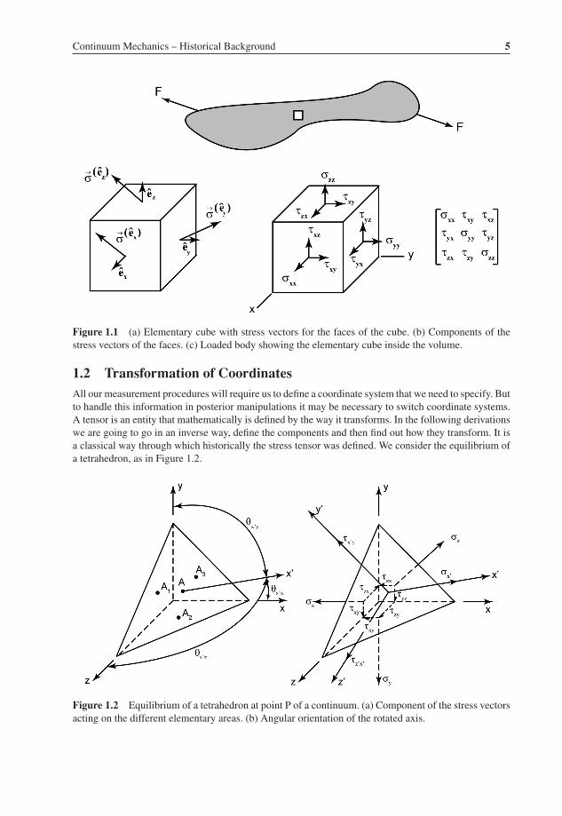
1.1 Definition of the Concept of StressThe concept of stress is one of the building blocks of continuum mechanics. The stress vector at a pointis defined as a force per unit area as in
�� = lim �F�A
�A → 0(1.1)
where �F denotes the force acting on �A, this vector depends on the orientation of the surface definedby its normal. This vector is not necessarily normal to the surface.
The stress vector does not characterize the state of stress at a given point of the space in the continuum.The state of stress is characterized by a more complex quantity know as the stress tensor �ij. The stresstensor has nine components, of which only six are independent. The stress components are representedin a Cartesian system of coordinates by the stress Cartesian tensor that was originally introducedby Cauchy.
[�] =∣∣∣∣∣∣
�x �xy �xz�yx �y �yz�zx �zy �z
∣∣∣∣∣∣
(1.2)
The cube shown in Figure 1.1 represents the stress tensor at a point with its nine components(
�ij = �ji)
.This definition has the ambiguity in language we have pointed out before. Figure 1.1 represents a cube
in the continuum, but as we said before ideally it represents a system of three mutually perpendicularplanes that go through a point. Each of these planes are defined by their normals, in this case the basevector of an orthogonal Cartesian system x, y, z. At each face of the cube there is a resultant stress vector
that we have represented by→�
(ei )with i = x, y, z. As can be seen these vectors are not perpendicular
to the faces of the cube. The components of the stress tensor are the projections of the stress vectorsin the direction of the coordinate axis. Mathematically, the tensor is a point function that, according tocontinuum mechanics, is continuous and has continuous derivatives up to the third order. However, whenwe want to measure it we need to make the measurement in a finite volume. If the finite volume is toosmall compared to the representative volume, what we measure will appear to us as a random quantity.The fact that we have talked about measuring a stress tensor is again an ambiguity in language. There isno way to measure stresses directly, we will be able to measure deformations and changes of geometryfrom which we will compute the values of stresses.
P1: SFN/XYZ P2: ABCJWST117-c01 JWST117-Sciammarella February 8, 2012 23:39 Printer Name: Yet to Come
Continuum Mechanics – Historical Background 5
Figure 1.1 (a) Elementary cube with stress vectors for the faces of the cube. (b) Components of thestress vectors of the faces. (c) Loaded body showing the elementary cube inside the volume.
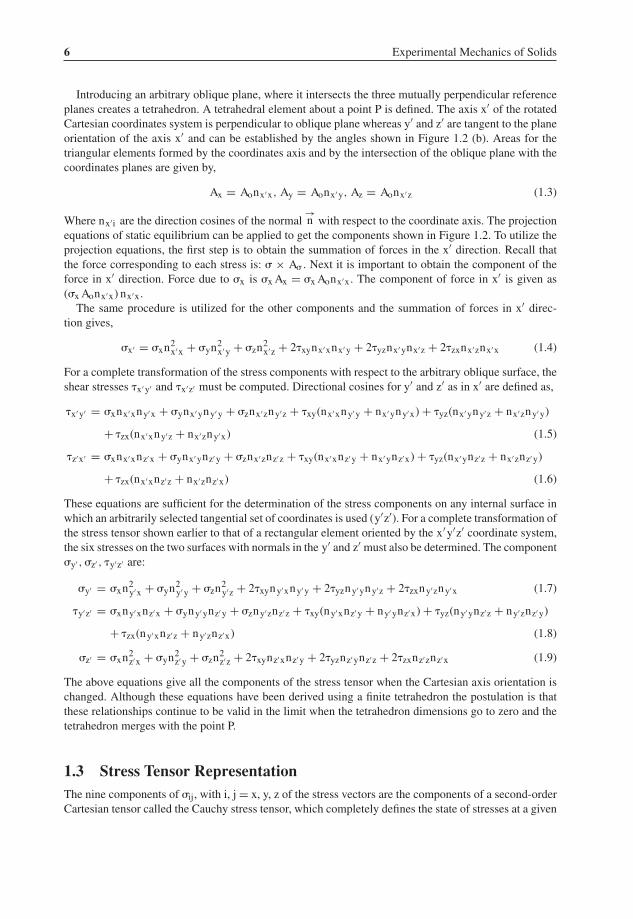
1.2 Transformation of CoordinatesAll our measurement procedures will require us to define a coordinate system that we need to specify. Butto handle this information in posterior manipulations it may be necessary to switch coordinate systems.A tensor is an entity that mathematically is defined by the way it transforms. In the following derivationswe are going to go in an inverse way, define the components and then find out how they transform. It isa classical way through which historically the stress tensor was defined. We consider the equilibrium ofa tetrahedron, as in Figure 1.2.
Figure 1.2 Equilibrium of a tetrahedron at point P of a continuum. (a) Component of the stress vectorsacting on the different elementary areas. (b) Angular orientation of the rotated axis.
P1: SFN/XYZ P2: ABCJWST117-c01 JWST117-Sciammarella February 8, 2012 23:39 Printer Name: Yet to Come
6 Experimental Mechanics of Solids
Introducing an arbitrary oblique plane, where it intersects the three mutually perpendicular referenceplanes creates a tetrahedron. A tetrahedral element about a point P is defined. The axis x′ of the rotatedCartesian coordinates system is perpendicular to oblique plane whereas y′ and z′ are tangent to the planeorientation of the axis x′ and can be established by the angles shown in Figure 1.2 (b). Areas for thetriangular elements formed by the coordinates axis and by the intersection of the oblique plane with thecoordinates planes are given by,
Ax = Aonx′x, Ay = Aonx′ y, Az = Aonx′z (1.3)
Where nx′i are the direction cosines of the normal→n with respect to the coordinate axis. The projection
equations of static equilibrium can be applied to get the components shown in Figure 1.2. To utilize theprojection equations, the first step is to obtain the summation of forces in the x′ direction. Recall thatthe force corresponding to each stress is: � × A� . Next it is important to obtain the component of theforce in x′ direction. Force due to �x is �x Ax = �x Aonx′x. The component of force in x′ is given as(�x Aonx′x) nx′x.
The same procedure is utilized for the other components and the summation of forces in x′ direc-tion gives,
�x′ = �xn2x′x + �yn2
x′ y + �zn2x′z + 2�xynx′xnx′ y + 2�yznx′ ynx′z + 2�zxnx′znx′x (1.4)
For a complete transformation of the stress components with respect to the arbitrary oblique surface, theshear stresses �x′ y′ and �x′z′ must be computed. Directional cosines for y′ and z′ as in x′ are defined as,
�x′ y′ = �xnx′xny′x + �ynx′ yny′ y + �znx′zny′z + �xy(nx′xny′ y + nx′ yny′x) + �yz(nx′ yny′z + nx′zny′ y)
+ �zx(nx′xny′z + nx′zny′x) (1.5)
�z′x′ = �xnx′xnz′x + �ynx′ ynz′ y + �znx′znz′z + �xy(nx′xnz′ y + nx′ ynz′x) + �yz(nx′ ynz′z + nx′znz′ y)
+ �zx(nx′xnz′z + nx′znz′x) (1.6)
These equations are sufficient for the determination of the stress components on any internal surface inwhich an arbitrarily selected tangential set of coordinates is used (y′z′). For a complete transformation ofthe stress tensor shown earlier to that of a rectangular element oriented by the x′y′z′ coordinate system,the six stresses on the two surfaces with normals in the y′ and z′ must also be determined. The component�y′ , �z′ , �y′z′ are:
�y′ = �xn2y′x + �yn2
y′ y + �zn2y′z + 2�xyny′xny′ y + 2�yzny′ yny′z + 2�zxny′zny′x (1.7)
�y′z′ = �xny′xnz′x + �yny′ ynz′ y + �zny′znz′z + �xy(ny′xnz′ y + ny′ ynz′x) + �yz(ny′ ynz′z + ny′znz′ y)
+ �zx(ny′xnz′z + ny′znz′x) (1.8)
�z′ = �xn2z′x + �yn2
z′ y + �zn2z′z + 2�xynz′xnz′ y + 2�yznz′ ynz′z + 2�zxnz′znz′x (1.9)
The above equations give all the components of the stress tensor when the Cartesian axis orientation ischanged. Although these equations have been derived using a finite tetrahedron the postulation is thatthese relationships continue to be valid in the limit when the tetrahedron dimensions go to zero and thetetrahedron merges with the point P.
1.3 Stress Tensor RepresentationThe nine components of �ij, with i, j = x, y, z of the stress vectors are the components of a second-orderCartesian tensor called the Cauchy stress tensor, which completely defines the state of stresses at a given

![Mechanics of Solids [3 1 0 4] CIE 101 / 102 First Year B.E ...icasfiles.com/mechanics of solids/notes/slides/1... · Mechanics of Solids PART-I PART-II Mechanics of Deformable Bodies](https://static.fdocuments.in/doc/165x107/60e4e466746b7501e128b225/mechanics-of-solids-3-1-0-4-cie-101-102-first-year-be-of-solidsnotesslides1.jpg)