Alti Sigma Ve Istatistiksel Uygulamalari Six Sigma and Statistical Tools
Upload
ali-osman-oencelCategory
view
63download
2
STATISTICAL PHYSICS, SEiSMOGENESIS, AND SEISMIC HAZARD
lan Main
Department of Geology and Geophysics Grant Institute, University of Edinburgh Edinburgh, Scotland
Abstract. The scaling properties of earthquake popu- lations show remarkable similarities to those observed at
or near the critical point of other composite systems in statistical physics. This has led .to the development of a variety of different physical models of seismogenesis as a critical phenomenon, involving locally nonlinear dynam- ics, with simplified rheologies exhibiting instability or avalanche-type behavior, in a material composed of a large number of discrete elements. In particular, it has been suggested that earthquakes are an e•ample of a "self-organized critical phenomenon" analogous to a sandpile that spontaneously evolves to a critical angle of repose in response to the steady supply of new grains at the summit. In this stationary state of marginal stability the distribution of avalanche energies is a power law, equivalent to the Gutenberg-Richter frequency-magni- tude law, and the behavior is relatively insensitive to the details of the dynamics. Here we review the results of some of the composite physical models that have been developed to simulate seismogenesis on different scales during (1) dynamic slip on a preexisting fault, (2) fault growth, and (3) fault nucleation. The individual physical models share some generic features, such as a dynamic energy flux applied by tectonic loading at a constant strain rate, strong local interactions, and fluctuations generated either dynamically or by fixed material heter- ogeneity, but they differ significantly in the details of the assumed dynamics and in the methods of numerical solution. However, all exhibit critical or near-critical behavior, with behavior quantitatively consistent with many of the observed fractal or multifractal scaling laws of brittle faulting and earthquakes, including the Guten-
berg-Richter law. Some of the results are sensitive to the details of the dynamics and hence are not strict examples of self-organized criticality. Nevertheless, the results of these different physical models share some generic sta- tistical properties similar to the "universal" behavior seen in a wide variety of critical phenomena, with sig- nificant implications for practical problems in probabi- listic seismic hazard evaluation. In particular, the notion of self-organized criticality (or near-criticality) gives a scientific rationale for the a priori assumption of "sta- tionarity" used as a first step in the prediction of the future level of hazard. The Gutenberg-Richter law (a power law in energy or seismic moment) is found to apply only within a finite scale range, both in model and natural seismicity. Accordingly, the frequency-magni- tude distribution can be generalized to a gamma distri- bution in energy or seismic moment (a power law, with an exponential tail). This allows extrapolations of the frequency-magnitude distribution and the maximum credible magnitude to be constrained by observed seis- mic or tectonic moment release rates. The answers to
other questions raised are less clear, for example, the effect of the a priori assumption of a Poisson process in a system with strong local interactions, and the impact of zoning a potentially multifractal distribution of epicen- tres with smooth polygons. The results of some models show premonitory patterns of seismicity which could in principle be used as mainshock precursors. However, there remains no consensus, on both theoretical and practical grounds, on the possibility or otherwise of reliable intermediate-term earthquake prediction.
1. INTRODUCTION
The prediction of individual earthquakes has long proven to be one of the "holy grails" of geophysics [Macelwane, 1946; Richter, 1958; Suzuki, 1982; Turcotte, 1991; Johnston, 1996]. Of course, we would like to be able to predict the exact location, size, and time of a future event (i.e., before it happens), within narrow limits or error bounds [Wood and Gutenberg, 1935], and at a level of statistical significance above the null hypoth- esis of a random Poisson process, but is it possible?
Scholz [1990a] has pointed out that there are practical problems in identifying precursors at a useful level of statistical significance. For example, in recent exercises in identifying statistically significant precursors accord- ing to a precise set of criteria, no clear positive examples were found [Wyss, 1991; Geller, 1996]. However, three examples were accepted, on the balance of evidence, onto a "preliminary list of significant precursors" [Wyss, 1991]. The absence of clear-cut precursors may be due to either of two reasons: (1) reliable earthquake precursors do generally exist on a timescale useful for predictive
Copyright 1996 by the American Geophysical Union.
8755-1209/96/96 RG-02808515.00
ß 433 ß
Reviews of Geophysics, 34, 4 / November 1996 pages 433-462
Paper number 96RG02808

434 ß Main: STATISTICAL PHYSICS AND SEISMIC HAZARD 34, 4 / REVIEWS OF GEOPHYSICS
purposes, but our instrumentation is currently insuffi- cient to record them, or (2) they do not generally exist owing to the underlying nonlinear physics [e.g., Brune, 1979; Kagan, 1994a]. Nonlinear dynamics implies ex- treme sensitivity to initial conditions, making accurate long-term prediction potentially difficult or impossible, because we can measure such conditions on potential earthquake nucleation sites only indirectly and incom- pletely. Therefore it is possible, many would say even likely, that the reliable prediction of individual earth- quakes, on a timescale of practical use for ordered evacuation, may prove to be an inherently unattainable goal.
In contrast, there has been a great deal of progress in recent years in the analysis of the statistical physics of seismogenesis as a process, notably in explaining the role of dynamic complexity in generating the rich order and pattern we see in the occurrence of populations of faults and earthquakes on a variety of scales. The aim of this article is to review some of this progress and to assess, even at this early stage, the impact of this relatively new paradigm on some practical problems in seismology. The emphasis is on probabilistic seismic hazard, which relies on the statistics of earthquake populations, rather than on the prediction of individual earthquakes.
We begin with a brief summary of some basic con- cepts in statistical physics and nonlinear dynamics and then summarize some of the important scaling proper- ties to be addressed in the phenomenology of earth- quakes. The section on statistical physics and seismogen- esis includes a description of recent results obtained from composite physical models of (1) earthquake pop- ulations in the plane of an existing fault, (2) the devel- opment of large-scale earthquake faults, and (3) the nucleation and growth of smaller faults. The influence of pore fluids as an extra source of complexity is discussed with primary relevance to fault nucleation and induced seismicity. The interested reader is referred to the on- going debate of the mechanical role of pore fluids in larger-scale processes introduced by Hickman et al. [1995]. In the final section we discuss some of the prac- tical implications of the statistical physics of earthquakes for probabilistic seismic hazard analysis. For reference, a glossary of specialized terms follows the main text.
1.1. Some Basic Concepts in Statistical Physics and Nonlinear Dynamics
Statistical physics, or statistical mechanics, is the branch of condensed matter physics dealing with the physical properties of macroscopic systems consisting of a large number of elements (classically, atoms or mole- cules). This approach has been applied to various prob- lems with analytical solutions in the equilibrium thermo- dynamics of composite systems, for example the behavior of ideal gases and paramagnetism [e.g., Mandl, 1988]. Examples of analytical models for the statistical mechanics of earthquakes are given by Main and Burton
[1984, 1986], Lomnitz-Adler [1985], Rundle [1988, 1989a, b, 1993], and Sornette and Sornette [1989].
More recently, the advent of powerful computers has permitted the study of a wider variety of complex sys- tems, involving a competition of local interactions and random fluctuations in a composite material composed of a large, but finite, number of discrete elements. Ex- amples of relevance to this article include the Ising model for magnetism [Bruce and Wallace, 1989] and resistor network models in electrical conduction [Van- neste and Sornette, 1992]. The application of this rela- tively new branch of computational statistical physics to problems in seismogenesis is one of the prime topics of this review.
Nonlinear dynamics is the branch of mathematics dealing with dynamical differential (or finite difference) equations, with nonlinear terms representing the feed- back loops often seen in natural systems. The mathe- matical problem is deterministic in the sense that we are dealing with dynamical equations that are known ex- actly. For linear dynamics such determinism results a completely predictable behavior. However, even for very simple nonlinear systems, with only a few degrees of freedom (i.e., the number of independent dynamical variables), we find a surprising range of behavior, from the completely regular and predictable to the completely chaotic and unpredictable [e.g., Tsonis, 1992]. Such de- terministic chaos has been applied in simplified models of phenomena as diverse as population dynamics in biology and earthquake dynamics in geophysics [Huang and Turcotte, 1990a, b; Scholz, 1990b; Turcotte, 1992].
The idea of deterministic chaos is usually applied to simple systems with only a few degrees of freedom and has been used predominantly as a forward modeling tool. The main reason for this is that it has proven extremely difficult to invert for the underlying dynamics from natural data with a large random component, for example, even for the basic problem of determining the number of degrees of freedom in the system [Tsonis, 1992; Ruelle, 1994]. Similar difficulties have also been found in inverting for the number of degrees of freedom in model earthquake sequences [McCloskey and Bean, 1992]. More recently, attention in this field has concen- trated on nonlinear systems with many degrees of free- dom: the study of dynamic complexity [e.g., Nicolis and Prigogine, 1989].
One of the properties of nonlinear systems is their capacity to exhibit self-organization•the spontaneous emergence of configurational order or pattern•in a variety of natural systems driven far from equilibrium. For example, Nicolis [1989] explains how patterns of thermal convection rolls and chemical zoning emerge spontaneously from solutions to the relevant nonlinear dynamical equations for convection and reaction-advec- tion-diffusion processes. The application of these spe- cific examples to problems in geophysics (mantle con- vection) and geochemistry (zoning) are reviewed respectively by Turcotte [1992] and Ortoleva [1994], who

34, 4 /REVIEWS OF GEOPHYSICS Main: STATISTICAL PHYSICS AND SEISMIC HAZARD ß 435
demonstrate that similar ordered patterns can evolve under appropriate conditions in the Earth. However, much of the spatial order in geophysical systems does not take the form of patterns with a characteristic length. For example, at high Rayleigh number, convection be- comes turbulent, and the regular pattern of similar-sized cells gives way to a more disordered pattern involving eddies of motion on all scales. As an analogue, Kagan [1992] refers to seismicity as the "turbulence of solids."
The geometrical properties of such hierarchical dis- tributions (turbulence, earthquake populations) are of- ten scale-invariant or self-similar (the words are often used interchangeably in the literature, but see below). Such systems have no characteristic length and have the same broad appearance at all magnifications. This fun- damental scaling property is the basis for the definition of the fractal geometry of natural systems. Mandelbrot [1983, p. 15] defines a fractal set strictly in terms of its topology: "A fractal is a set for which the Haussdorff- Besicovitch dimension strictly exceeds the topological (Euclidean) dimension." This strict mathematical defi- nition is not the one in common use in geology and geophysics. Instead, Turcotte [1992] defines a fractal set as one in which the number N of objects or fragments of length L scale as a power law of exponent D (equation (1) below). Turcotte's definition includes all of the frac- tal sets defined by Mandelbrot but also includes scale invariance for sets in which there is no information on
the location of elements in the set, for instance, the frequency-length distribution for seismic sources, or the scaling of hierarchical models for fragmentation.
Some fractal sets exhibit scale-invariant properties that are not isotropic. For example, the scaling proper- ties of a coastline (horizontal section) are different from those of ground elevation (vertical section), although both exhibit scale invariance in their own plane. Isotro- pic scale invariance is self-similar, meaning that objects appear similar in all directions at all scales. In contrast, self-arline objects, when seen at different magnification, appear self-similar only with some anisotropic magnifi- cation, for example, a vertical exaggeration of scale (illus- trated by Power and Tullis [1991, Figure 2]). The roughness of fault and fracture surfaces has been interpreted with methods assuming both self-similar [Aviles et al., 1987] and self-affine [Brown and Scholz, 1985; Scholz and Aviles, 1986; Schmittbuhl et al., 1995] geometry. Power and Tullis [1991, 1995] concluded that, for natural fault and fracture sur- faces on a scale range from 10 !xm to 40 m, "approxi- mate" self-similarity holds when the data are interpreted over the whole bandwidth, but self-aifine behavior is more appropriate within smaller wavelength bands.
Another complication is the existence of multifractal scaling, which has two related aspects. The first involves spatial variability, so that the overall scaling exponent of the whole set can be described in terms of a superposi- tion of smaller subsets with different individual scaling exponents oti. This phenomenon is well known in turbu- lence and can be quantified by plotting the "spectrum of
singularities," f(ot) [e.g., Feder, 1988, Figure 6.5], equiv- alent to the fractal dimensions of the subsets. Multifrac-
tal behavior cannot be established without a sufficiently broad band of observation. For example, Lovejoy and Schertzer [1991] established the phenomenon for cloud patterns and rainfall over a bandwidth of nine orders of magnitude (10-3-106 m).
The second aspect of multifractals is related to the scaling of "mass" weightings of objects in the set at different magnifications. For example, in a set of one- dimensional lines, the mass weighting in a generalized "box-counting" algorithm is the product of the linear density and the total line length enclosed in a box in a grid of scale length L [Grassberger, 1983; Feder, 1988]. Fractal dimensions D q are then calculated by counting the number of boxes containing a line, weighted by the mass raised to the power q. This procedure is equivalent to estimating the different moments q of a probability distribution. For q : 0 there is no mass weighting, so Do, sometimes known as the "capacity" dimension, is equivalent to Mandelbrot's [1983] fractal dimension. The higher-order dimensions include the "information" di- mension D 1 and the "correlation" dimension D 2 [Feder, 1988]. The multifractal spectrum Dq can be related math- ematically to f(ot) by a Legendre transform [Halsey et al., 1986; Geilikman et al., 1990], so the mass clustering is directly related to the spatial variability (see, for example, Feder [1988, Figures 6.7, 6.8, 6.9]). The multifractal spec- trum can also be calculated by weighting according to other criteria. In describing tectonic deformation, for example, it is often useful to weight according to the cumulative displacement on faults rather than a mass based on the linear density [e.g., Davy et al., 1992; Cowie et al., 1995].
The prime use of multifractals is in quantifying the degree of concentration, clustering properties, and in- termittency in the fractal set of interest. Multifractal measures have been found to describe the geometrical properties of faults, fractures, and earthquakes, includ- ing seismicity in Pamir, the Caucasus, and California [Geilikman et al., 1990]; aftershocks of the 1992 Erzincan (Turkey) earthquake [Legrand et al., 1996]; patterns of faults in analogue laboratory models of layered litho- sphere deformation [Davy et al., 1992]; the distribution of opening displacements in fractures recorded in well logs [Belfield, 1994]; and the concentration of plastic deforma- tion in shear bands in rocks [Poliakov and Herrmann, 1994].
Another measure of spatial clustering is the two-point correlation dimension, determined by the distribution of spacing between points [Grassberger and Procaccia, 1983]. This method has been applied to demonstrate that the clustering properties of laboratory hypocenters [Hirata et al., 1987] and epicentral data in natural seis- micity [Kagan and Knopoff, 1980; Hiram, 1989; Hender- son et al., 1992] are fractal in nature. Hirata and Imoto [1991] applied a mass weighting to the distribution of spacings and showed that the two-point spacing statistics in the Kanto region of Japan could be described by a multifractal set. Eneva [1996] applied this generalized

436 ß Main: STATISTICAL PHYSICS AND SEISMIC HAZARD 34, 4 / REVIEWS OF GEOPHYSICS
(a) California faults showing evidence of activity in latest 15m.y. ( Howard & others,
__--•'- .• , / .•.
{b) •osht-e8oyez eorthq.oke fo.lt, Iro. {Tcholenko, l•70}
-- m•/J • /'•1 lOOm (c) Clay deformation in a Reidel shear experiment ( Tchalenko, 1970 )
I I
IOmm
(d) Detail of shear box experiment ( Tchalenko, 1970)
I Imm I
Figure 1. Traces of fault populations on a range of scales, from laboratory experiments (Figures l c and l d) to plate-rupturing faults such as the San Andreas (Figure la) (after Main et al. [1990]; original data from Tchalenko [1970], Howard et al. [1978], and Shaw and Gartner [1986]). The fault patterns are scale-invariant in the sense that without scale bars it would be dill]cult to tell them apart.
technique to mining-induced seismicity in Canada but concluded that incomplete sampling often present in seismicity data may introduce some spurious multifractal effects that do not reflect the underlying physical pro- cess. Similarly, Oncel et al. [1995] concluded that system- atic changes in the measured correlation dimension as a function of time in northern Turkey can be assigned to temporal changes in instrumental deployment rather than an underlying physical cause.
The applicability of fractals to geology and geophysics is the subject of a burgeoning literature, including text- books [e.g., Turcotte, 1992; Korvin, 1992; Xie, 1993] as well as special volumes in the form of collections of papers [e.g., Schertzer and Lovejoy, 1991; Kruhl, 1994; Barton and La Pointe, 1995]. However, the prime aim of this review is not to examine the detailed applicability of fractal measures to fault nucleation, fault growth, and seismogenesis. Instead we evaluate the implications of a new class of physical models that have recently been developed to describe their scaling properties. This new
paradigm involves the statistical physics of a system with many degrees of freedom, with populations of individual elements obeying the local nonlinear constitutive rules of fracture or friction. It is therefore an example of dynamic complexity rather than low-dimensional chaos. Of particular interest is how the extraordinarily ordered pattern of seismogenic deformation on Earth might have been first developed and then maintained, using con- cepts developed not in geology or geophysics but in the statistical physics of critical point phenomena. First we briefly summarize some of the phenomenology of earth- quakes and fault populations to which this class of model is primarily addressed.
1.2. Phenomenology of Earthquakes and Fault Populations
Any general theory for the statistical physics of fault- ing and earthquakes has to explain the following empir- ical facts or relations concerning their scaling properties:
1. Fault populations are broadly scale-invariant over

34, 4 / REVIEWS OF GEOPHYSICS Main' STATISTICAL PHYSICS AND SEISMIC HAZARD ß 437
several orders of magnitude (e.g., Figure 1), and as a consequence have power law length distributions (Fig- ure 2) of the form
N(L ) = AL-ø, (1)
where N here is the number of faults of length exceeding L, D is the scaling exponent of the length distribution (the slope on a log-log plot), and A is a constant [King, 1983; Shaw and Gartner, 1986; Heifer and Bevan, 1990; Main et al., 1990; Sornette and Davy, 1991; Turcotte, 1992].
2. Earthquake frequency-magnitude statistics also imply power law scaling via the Gutenberg-Richter law for earthquake recurrence [Gutenberg and Richter, 1954]
log N = a - bm, (2)
where we shall take N to be an incremental frequency of occurrence of earthquakes of magnitude in the range rn _+ 8m/2 (usually 8m = 0.1) and a and b are constants. The negative slope b is usually referred to as the seismic "b value." The Gutenberg-Richter law cor- responds to a power law distribution of fault length, seismic moment or seismic energy. Figure 3 [after Main and Burton, 1984; Turcotte, 1992] shows an example from southern California.
3. Earthquakes have a relatively constant and rela- tively small stress drop over a wide range of scales during
z
ß California fault system
-i- Dasht-e Bayez fault Iran
• o Clay deformation Reidel - shear experiment
• /• details of shear box experiment
Slope= -2 • - \
ß ,-i-
SIo
I
0 I
log L
Figure 2. Frequency-length distribution (log-log plot) of the faults determined from Figure 1 (after Main et al. [1990]; original data from Tchalenko [1970], Howard et al. [1978], and Shaw and Gartner [1986]). The data have been renormalized so that data on different scales can be plotted together. The solid straight line for these two-dimensional maps is consistent with a power law size distribution of length of exponent D - 1. The dashed line represents a slope of D - 2, the usual case for earthquake source dimensions when sampled in three dimen- sions [Turcotte, 1992].
2.0
1.0
• 0.0-
o -1.0.
-3.0 4.0 9.0 5.0 6.0 7.0 8.0
Magnitude M s
Figure 3. Discrete frequency-magnitude distribution (log lin- ear plot) of earthquakes in southern California [after Main and Burton, 1984]. The solid line represents a maximum entropy fit to the data constrained by the long-term moment release rate. The result fits both the short-term instrumental data (several decades, open areas) and the longer-term palaeoseismic recur- rence (over 2 millennia, shaded area) in this case.
dynamic slip (3 MPa compared with tectonic and litho- static stresses in the crust of the order of 10-100 MPa). Figure 4 [after Abercrombie and Leary, 1993; Abercrom- bie, 1995] shows a composite of several data sets exhib- iting this property on a wide range of scales, from 10 m to 100 km. Although scale invariance of stress drop is
1 0 21 I ' ' ' i•••'e ,•' •Cajon Pass Borehole ,,,•. ',, 1 019 ß Various Combined Studies
•' .• .-... ß Z•. 1017 . ß ß 1,
.e- ß • eee ß
•0
10 TM
Lines of mnstant stress drop {bars) 109
5 10 102 10 a 10 • 10 • Source Dimension (m)
Figure 4. Scaling of seismic moment as a function of source size (log-log plot) after Abercrombie [1995], who also gives the original references for the combined studies indicated. The solid lines represent the scaling predicted at different stress drops (in bars) from a simple dislocation model for the seismic source. The high-resolution borehole data from the Cajon Pass borehole (open triangles) show no strong systematic difference from earthquake data at larger scales (solid circles) within the scatter of the data; i.e., there is no systematic "fmax" effect.

438 ß Main: STATISTICAL PHYSICS AND SEISMIC HAZARD 34, 4 / REVIEWS OF GEOPHYSICS
10 0
101
b••"• ß Sec..ondary [///•/ ß Tertiary
10 4 I I I I 1 2 4 8 16 32
r, mm
Figure 5. Cumulative probability (Pr) distribution that hypo- centers are separated by a linear distance R less than a char- acteristic scale r (log-log plot) (after Main [1992a]; original data from Hirata et al. [1987]). The data comprise hypocentral locations of acoustic emissions in rock samples during the three phases (primary, secondary, and tertiary) of a creep test in initially intact crystalline rock. The slope of the solid straight lines is equivalent to the correlation dimension, which de- creases as deformation progresses (as indicated by the arrow in the bottom left corner).
indicated by the data following the theoretical straight lines on the figures, there remains a considerable real scatter in the data above the level of measuring uncer- tainty [Abercrombie, 1995].
4. Fault and fracture breaks are rough, with self- arline or self-similar scaling [Brown and Scholz, 1985; Scholz, 1990a; Power and Tullis, 1991, 1995; Schmittbuhl et al., 1995].
5. Earthquake populations in diverse tectonic zones exhibit spatial variability, clustering, and intermittency, quantitatively consistent with multifractal scaling [Geil- ikman et al., 1990; Hirata and Imoto, 1991].
6. The distribution of spacings of hypocentral loca- tions of earthquakes and laboratory acoustic emissions are power law in both space [Kagan and Knopoff, 1980; Hirata, 1989; Henderson et al., 1992] and time [Turcotte, 1992]. Figure 5 [after Hirata et al., 1987] shows an example from laboratory hypocentral data during the three stages of a creep experiment.
7. Earthquakes have aftershock sequences that de- cay at a rate R(t) determined by Omori's law, general- ized by Utsu [1961] in the form
= o/(t + to)" (3)
wherep is a power law index, and R 0 and t o are constants to be determined from the data.
In addition to these scaling properties we make the following observation:
8. seismicity can be induced by stress perturbations smaller than the stress drop in individual events. These may be due to previous earthquakes occurring at rela-
tively great distances [Hill et al., 1993; Stein et al., 1994; Kagan, 1994b; Gomberg and Davis, 1996; Stark and Davis, 1996], or to changes in local pore fluid pressure through man-made activity [Segall, 1989]; i.e., earth- quakes can be "triggered" [Brune, 1979].
In the two-dimensional map views of Figure 1 the scaling exponent of the length distribution is D - 1 (Figure 2). In contrast, natural seismic sources occur in a three-dimensional volume, and the inferred distribu- tion of fault lengths implies D = 2 [King, 1983; Turcotte, 1992]. Thus the dimensionality of the sampling tech- nique exerts a strong influence on the measured fractal dimension. The multifractal clustering of faults and earthquake locations is consistent with two important general observations, namely, (1) the observed concen- tration of seismic moment or energy release on large, dominant faults and (2) the presence of some seismicity everywhere, including areas remote from plate boundaries.
2. STATISTICAL PHYSICS AND SEISMOGENESIS
In this section we review some of the results of a
plethora of physical models for seismogenesis as a crit- ical, or self-organized critical, phenomenon. Before do- ing this it is worthwhile to discuss what is meant by a "model" in such cases. There are two stages in reducing what happens in a natural composite material to some- thing that is computationally or analytically tractable. The first is to develop a generic "conceptual model," which simplifies the behavior of the physical system to an idealized version that preserves the essential features of the process to be modeled but is capable of numerical or analytical solution. This is the stage where most of the important assumptions regarding the process are made. The second step is to develop a specific numerical or computational model to solve the set of equations that describe the conceptual model, which may involve fur- ther simplification. We therefore distinguish in the text between a conceptual model and a numerical model, using the term "physical model" or simply "model" to imply the resultant of both steps. First we examine how such procedures have shed light on other systems in statistical physics.
2.1. Critical Point Phenomena
One of the branches of statistical physics where power law scaling with long-range correlations is produced is at or near the critical point in order-disorder phase transi- tions [Ma, 1976; Bruce and Wallace, 1989]. For example, at the critical point in the phase transition between a liquid (more ordered state) and a gas (more disordered state), the density difference between two phases van- ishes. In the more ordered state the interactions between
molecules (van der Waal's forces) dominate, in contrast to the thermal fluctuations, which dominate in the more disordered state. The critical point for this phase tran-

34, 4 / REVIEWS OF GEOPHYSICS Main: STATISTICAL PHYSICS AND SEISMIC HAZARD ß 439
sition occurs at a precise combination of pressure and temperature for a given material.
Similar critical point behavior is seen when a mag- netic material is cooled below its Curie temperature. Here correlated "domains," or clusters of large con- nected areas with coherent magnetisation, emerge from the chaos seen at higher temperatures. The Curie tem- perature also represents a critical point between ordered behavior dominated by spin-spin interactions at lower temperatures, and disordered thermal fluctuations at higher temperatures. Similar behavior is seen in a variety of critical point phenomena, giving rise to the notion of "universality," where diverse physical systems share sim- ilar (in some cases exactly the same) scaling properties near their critical points [Ma, 1976; Bruce and Wallace, 1989]. It is therefore informative to consider one exam- ple in a little detail before progressing to the physics of earthquake populations.
In so-called "Ising" models for magnetism, the con- ceptual model takes the form of a regular array of individual magnetized elements, which interact solely with their neighboring elements. The individual mag- netic elements may be magnetized either parallel or antiparallel to the external generating field, generating a binary or Boolean field. The physical problem is thus reduced to a conceptual problem in the form of a cellu- lar automaton, which similar in many respects to a finite element model working on a regular grid and which is capable of numerical solution. The numerical solution involves replacing the physics of the spin exchange forces with local numerical "rules" that approximate their behavior, for example, neglecting the effect of weaker long-range interactions. Wolfram [1984, 1986] describes several examples of computational cellular au- tomata, designed to model the behavior of a variety of complex systems. A common feature of cellular autom- ata, with differing local rules, is that they produce long- range order that emerges spontaneously through dy- namic feedback and self-organization.
The results of the Ising model show the spontaneous development of organized magnetic domains at the Cu- rie temperature, with a power law size distribution, and fractal scaling of the rough domain walls [Bruce and Wallace, 1989, Figure 8.2]. Above the critical point, thermal fluctuations dominate, so the behavior is ran- dom or chaotic, and no ordered pattern is generated. As the temperature is reduced in the model, the local in- teractions begin to take effect, and organized clusters of aligned spins begin to emerge in the results. At the critical point To, domains of positive and negative mag- netism precisely cancel, and no additional external mag- netic field is generated. Below the critical point (T < T 0 increasingly regular magnetic domains are generated parallel to the external field. As a consequence, the "order parameter" (defined as the excess of areas with positive over negative magnetization) increases as the material cools, resulting in a systematic increase in the external field. In this example the critical point is bal-
anced exactly at the transition from order to disorder in the competition between local interactions and thermal fluctuations, a condition sometimes referred to as "on the edge of chaos." Nevertheless, the critical point is also associated with long-range correlations [Bruce and Wal- lace, 1989, Figure 8.3] and the disappearance of a char- acteristic length scale.
2.2. Self-Organized Criticality In the above examples the critical point is reached by
precise tuning of external variables (temperature and/or pressure). However, some complex physical systems can organize themselves spontaneously to the critical point, giving rise to the notion of a state of self-organized criticality. Thus the system organizes itself, not just into a patterned structure, but to the precise structure seen at the critical point, and then remains there apart from dynamic fluctuations. A state of self-organized criticality is therefore in some sense an attractor in the dynamics. Bak et al. [1988a, b] illustrated the concept by applying a cellular automaton model to the size distribution of
avalanches in a sandpile maintained at a critical angle of repose by the steady supply of new grains to the summit. The model system organizes itself spontaneously to the critical point (the critical angle of repose) and then remains there apart from dynamic fluctuations (the av- alanches). Although driven far from equilibrium by the constant flux of sand grains, the sandpile remains in a stationary state represented by a relatively constant an- gle of repose and power law scaling of the size distribu- tion of avalanches [Bak et al., 1988b]. However, minor events in the dynamics can start a chain reaction that can affect any number of elements in the system: i.e., the system exhibits "triggering" (observation 8 in section 1.2). After an initial transient, the system remains in a stationary but metastable state, balanced precisely be- tween a more ordered and a more disordered state, "at the edge of chaos" [Bak et al., 1988a,b]. A key property of this state is that the behavior of the system is relatively insensitive to the details of the dynamics, so that there is no need to tune the system externally (to "twiddle the knobs" [Bak et al., 1988b]) as in other examples of critical phenomena. Individual avalanches may be hard to predict because of the nonlinear physics, but the average properties (angle of repose, size distribution of avalanches, etc.) remain relatively constant in time.
A composite system in a state of self-organized criti- cality cannot reach a stable equilibrium but instead evolves dynamically from one metastable state to an- other. In the sandpile analogy the critical angle of re- pose, 0•, represents a stationary, but potentially unsta- ble, state achieved in the dynamic competition between the steady supply of potential energy (by addition of new grains) and the intermittent energy demand (from the sand avalanches). Over long timescales the angle of repose averages out at a constant value to maintain the critical slope, but short-term dynamic fluctuations are fundamental to maintaining this long-term metastability.
440 •, Main: STATISTICAL PHYSICS AND SEISMIC HAZARD 34, 4 / REVIEWS OF GEOPHYSICS
yv
•\o•. •"' K c KC
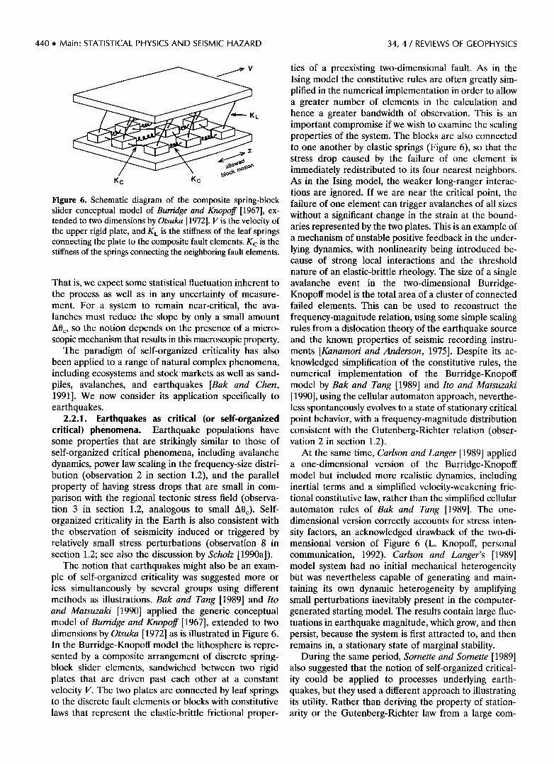
Figure 6. Schematic diagram of the composite spring-block slider conceptual model of Burridge and Knopoff [1967], ex- tended to two dimensions by Otsuka [1972]. l/is the velocity of the upper rigid plate, and Ki• is the stiffness of the leaf springs connecting the plate to the composite fault elements. Kc is the stiffness of the springs connecting the neighboring fault elements.
That is, we expect some statistical fluctuation inherent to the process as well as in any uncertainty of measure- ment. For a system to remain near-critical, the ava- lanches must reduce the slope by only a small amount A0c, so the notion depends on the presence of a micro- scopic mechanism that results in this macroscopic property.
The paradigm of self-organized criticality has also been applied to a range of natural complex phenomena, including ecosystems and stock markets as well as sand- piles, avalanches, and earthquakes [Bak and Chen, 1991]. We now consider its application specifically to earthquakes.
2.2.1. Earthquakes as critical (or self-organized critical) phenomena. Earthquake populations have some properties that are strikingly similar to those of self-organized critical phenomena, including avalanche dynamics, power law scaling in the frequency-size distri- bution (observation 2 in section 1.2), and the parallel property of having stress drops that are small in com- parison with the regional tectonic stress field (observa- tion 3 in section 1.2, analogous to small A0c). Self- organized criticality in the Earth is also consistent with the observation of seismicity induced or triggered by relatively small stress perturbations (observation 8 in section 1.2; see also the discussion by Scholz [1990a]).
The notion that earthquakes might also be an exam- ple of self-organized criticality was suggested more or less simultaneously by several groups using different methods as illustrations. Bak and Tang [1989] and Ito and Matsuzaki [1990] applied the generic conceptual model of Burridge and Knopoff [1967], extended to two dimensions by Otsuka [1972] as is illustrated in Figure 6. In the Burridge-Knopoff model the lithosphere is repre- sented by a composite arrangement of discrete spring- block slider elements, sandwiched between two rigid plates that are driven past each other at a constant velocity V. The two plates are connected by leaf springs to the discrete fault elements or blocks with constitutive
laws that represent the elastic-brittle frictional proper-
ties of a preexisting two-dimensional fault. As in the Ising model the constitutive rules are often greatly sim- plified in the numerical implementation in order to allow a greater number of elements in the calculation and hence a greater bandwidth of observation. This is an important compromise if we wish to examine the scaling properties of the system. The blocks are also connected to one another by elastic springs (Figure 6), so that the stress drop caused by the failure of one element is immediately redistributed to its four nearest neighbors. As in the Ising model, the weaker long-ranger interac- tions are ignored. If we are near the critical point, the failure of one element can trigger avalanches of all sizes without a significant change in the strain at the bound- aries represented by the two plates. This is an example of a mechanism of unstable positive feedback in the under- lying dynamics, with nonlinearity being introduced be- cause of strong local interactions and the threshold nature of an elastic-brittle rheology. The size of a single avalanche event in the two-dimensional Burridge- Knopoff model is the total area of a cluster of connected failed elements. This can be used to reconstruct the
frequency-magnitude relation, using some simple scaling rules from a dislocation theory of the earthquake source and the known properties of seismic recording instru- ments [Kanamori and Anderson, 1975]. Despite its ac- knowledged simplification of the constitutive rules, the numerical implementation of the Burridge-Knopoff model by Bak and Tang [1989] and Ito and Matsuzaki [1990], using the cellular automaton approach, neverthe- less spontaneously evolves to a state of stationary critical point behavior, with a frequency-magnitude distribution consistent with the Gutenberg-Richter relation (obser- vation 2 in section 1.2).
At the same time, Carlson and Langer [1989] applied a one-dimensional version of the Burridge-Knopoff model but included more realistic dynamics, including inertial terms and a simplified velocity-weakening fric- tional constitutive law, rather than the simplified cellular automaton rules of Bak and Tang [1989]. The one- dimensional version correctly accounts for stress inten- sity factors, an acknowledged drawback of the two-di- mensional version of Figure 6 (L. Knopoff, personal communication, 1992). Carlson and Langer's [1989] model system had no initial mechanical heterogeneity but was nevertheless capable of generating and main- taining its own dynamic heterogeneity by amplifying small perturbations inevitably present in the computer- generated starting 'model. The results contain large fluc- tuations in earthquake magnitude, which grow, and then persist, because the system is first attracted to, and then remains in, a stationary state of marginal stability.
During the same period, Sornette and Sornette [1989] also suggested that the notion of self-organized critical- ity could be applied to processes underlying earth- quakes, but they used a different approach to illustrating its utility. Rather than deriving the property of station- arity or the Gutenberg-Richter law from a large com-

34, 4 / REVIEWS OF GEOPHYSICS Main: STATISTICAL PHYSICS AND SEISMIC HAZARD ß 441
TABLE 1. Hallmarks of Self-Organized Criticality
Feature Sandpiles Earthquakes
Boundary condition Critical parameter Dynamic fluctuation
Power law distribution
constant "grain" rate repose angle 0c small fluctuations in angle
,50 << Oc avalahche volume or energy
constant strain rate
tectonic stress cr c small stress drop
source length, seismic moment, or energy (Gutenberg-Richter law)
puter-generated model of fluctuations and interactions, they assumed their existence a priori as a consequence of self-organized criticality. Using the assumption of sta- tionarity, they introduced the constraint of a constant energy flux and hence derived a probabilistic mean field (analytical) solution for the return periods of events of different energies in the form of a power law. (A dy- namic energy flux is crucial to the development of self- organizing systems, in contrast to the more static behav- ior of equilibrium thermodynamics [Nicolis, 1989]).
Some key assumptions are present in all of the com- putational models described above. For example, elastic strain energy is assumed to be supplied to the model fault from a remote boundary at a relatively constant strain rate, with the intermittent release of this stored energy resulting in earthquakes. The model fault is com- posed of a regular grid of individual discrete elements that interact solely through their nearest neighbors (al- though long-range interactions propagate dynamically in the one-dimensional model of Carlson and Langer [1989]). The average rate of energy input and release is then maintained relatively constant in a stationary state of marginal stability, analogous to the sandpile model, with power law scaling in the size distribution of earth- quake energies. These key properties can then be used, in simpler analytic models, to derive some statistical properties of earthquake recurrence [e.g., Sornette and Sornette, 1989]. Table 1 compares some of the essential features of the earthquake and sandpile models.
The different numerical variants of the Burridge- Knopoff conceptual model described above exhibit many of the empirical scaling relations observed in natural earthquake populations, but not all classes show evi- dence of true self-organized criticality [Rundle and Klein, 1993]. In particular, the strength of the permanent ma- terial heterogeneity and the plate-driving velocity both have significant effects on the resulting frequency-mag- nitude distribution in different realizations of the two-
dimensional version of the Burridge-Knopoff model [Rundle and Klein, 1993]. Permanent heterogeneity, or "quenched disorder" due to preexisting structure, is present in all geological systems, so it is reasonable to examine its influence on the dynamics. It is also reason- able to examine the effect of different plate-driving ve- locities, because spatial variations in driving velocity over 1.5 to 2 orders of magnitude are a feature of plate tectonics on Earth [e.g., DeMets, 1995]. The results
achieved by altering these variables are shown in Figure 7 [after Rundle and Klein, 1993]. All exhibit fractal scal- ing over a finite range, but only some show evidence of true self-organized criticality. For example, when the material heterogeneity is strong, the largest earthquakes never cross the entire area of the model fault surface, and the probability of occurrence of the largest events is reduced in comparison with an extrapolation of the Gutenberg-Richter trend (Figure 7a). Under these con- ditions the behavior is also sensitive to the plate-driving velocity (Figure 7a). Such systems are not strict examples of self-organized criticality because they are sensitive to external conditions. We shall refer to this generic class of models as "subcritical," in the sense that the largest avalanches do not cross the entire area of the model
fault. An equivalent statement is that the system remains below the percolation threshold, defined as the point at which the 'largest connected cluster of failed elements just spans the model grid [Stauffer and Aharony, 1994].
For weaker heterogeneity, with intermediate driving velocities, the behavior is both precisely critical and insensitive to the precise value of V (Figure 7b). This represents a true state of self-organized criticality, in which the system can generate and maintain its own dynamical heterogeneity, and whose scaling properties are relatively insensitive to the details of the dynamics. For even larger driving velocities a "supercritical" state may occur with an elevated probability of occurrence of large "characteristic" events (Figure 7c), similar to be- havior seen above the percolation threshold [Stauffer and Aharony, 1994, pp. 72-73]. A characteristic peak in the size distribution at large length scales is reminiscent of a first-order phase transition [Lomnitz-Adler et al., 1992; Ceva and Perazzo, 1993].
The range of behavior illustrated in Figure 7 is not specific to the details of the cellular automaton used by Rundle and Klein [1993]. For example Lomnitz-Adler [1993] examined 40 different classes of computational model for the statistical physics of earthquake popula- tions, based on different combinations of the following assumptions: total stress drop (crack model) or partial stress drop (frictional slip); homogeneous or random loading; the presence or absence of asperities; a short or long characteristic time for fracturing; and whether or not the dynamic strain energy (or stress) is conserved on the fault plane. All of these physical models were found to generate results within one of the three generic types

442 ß Main: STATISTICAL PHYSICS AND SEISMIC HAZARD 34, 4 / REVIEWS OF GEOPHYSICS
(a) (b) (c)
).10 -2 Z
:::3 10-4 o
n- 10 -6
:• 0-8
V=8
V=
%• i t I I i it • • t
10-1 10 o 101 10 2 10 3 10 4 CLUSTER SIZE
V= 0
10-1 10 0 101 10 2 10 3 10 4 CLUSTER SIZE
% I i i i % I I
10-1 10 0 101 10 2 10 3 10 4 CLUSTER SIZE
Figure 7. Frequency distribution of event cluster size from the results of applying the spring-block slider model of Figure 6, run under different initial and boundary conditions (log-log plot) (redrafted after Rundle and Klein [1993]), The cluster size S measures the connected area of failed elements, corresponding to an individual model earthquake. There is some statistical scatter, which results in a broadening of the lines encompassing the data for the rarer, larger events. The numerical model was run with (a) strong permanent heterogeneity with different plate velocity V (arbitrary units), (b) weak heterogeneity and relatively low or intermediate velocity V, and (c) weak heterogeneity and high V. The interested reader is referred to Rundle and Klein [1993] for more precise details of the numerical model. All of the results exhibit critical behavior, with power-law scaling (straight line slope) over a finite scale range. In Figure 7b the scaling properties of the system are power law right up to the largest events, with exponents that are relatively insensitive to the degree of external forcing. Only Figure 7b corresponds to a state of self-organized criticality. The behavior in Figure 7a may be termed "subcritical," and that in Figure 7c, "supercritical."
shown in Figure 7, but only a few classes produced precisely critical behavior (a Gutenberg-Richter law over all magnitudes (e.g., Figure 7b)). The same three generic types seen in Figure 7 can also be seen in the frequency-energy results of computational models for the dynamics of sandpiles [Ceva and Perazzo, 1993; Carl- son et al., 1993]. Lomnitz-Adler [1993] interprets this generic behavior in terms of different positions near the critical point, Ceva and Perazzo [1993] interpret it in terms of different positions around the percolation threshold, and Carlson et al. [1993] interpret it in terms of different solutions to the diffusion equation. This similarity of behavior in the results of such diverse phys- ical models is another example of the principle of uni- versality in such systems.
The results of Figure 7 show that the models must be "tuned" after all (at least to some extent) to produce self-organized criticality in the strict sense. That is, there is a finite range of starting states (i.e., dynamic variables and initial heterogeneity) in numerical models that then evolve spontaneously to a true state of self-organized criticality. Other combinations evolve to a stationary, near-critical state but are more sensitive to the details of
the dynamics. One of the prime variables that is used in practice to
tune the behavior of these numerical models is the
degree of conservation of energy following the failure of an element. For example, in order to produce a b value near 1 (observation 2 in section 1.2), most cellular au- tomaton models introduce an arbitrary degree of energy dissipation to the local constitutive rules. This is physi-
cally realistic because energy is lost to effects such as seismic radiation (radiation damping), deformation around the fault zone, or the movement of fluids, in addition to that lost in the generation of heat on the fault surface due to friction in the case of a partial stress drop. If all of the stored elastic energy were conserved, then the failure of a single element resulting in a stress drop Air would result in the loading of the four nearest neighbors in the cellular automaton by an amount Air/4 [e.g., Bak and Tang, 1989]. If the elastic energy is not conserved, the simplified technique used to represent such damping involves loading the neighbors by an amount otAtr/4, where ot < 1. Models with ot = 1 are termed "conservative," and those with ot < 1 are termed "nonconservative." Olami et al. [1992] examined the statistical properties of such numerical models and ob- served a systematic negative correlation between ot and the seismic b value. A b value near 1 is produced when ot = 0.8. In other words, the b value is sensitive to the input parameters, so that the results are sensitive to the details of the dynamics, in contrast to the strict require- ments of self-organized criticality [Kadanoff et al., 1989; Socolar et al., 1993].
The results of applying the various numerical imple- mentations of the Burridge-Knopoff conceptual model compare well with many other aspects of earthquake phenomenology. Examples include the spatiotemporal form of patterns of seismicity preceding large earth- quakes [Shaw et al., 1992], the phenomenon of seismic quiescence [Brown et al., 1991], Omori's law (in a gen- eralized form) for aftershocks and foreshocks (observa-
34, 4 / REVIEWS OF GEOPHYSICS Main: STATISTICAL PHYSICS AND SEISMIC HAZARD ß 443
tion 7 in section 1.2 [Shaw, 1993a]), the power law distribution of interevent times (observation 6 in section 1.2 [Matsuzaki and Takayasu, 1991], and the form of earthquake source spectra [Shaw, 1993b]. McCloskey [1993] and McCloskey et al. [1993] showed that the observed systematic changes in the b value at high mag- nitude could be explained by the effect of fault segmen- tation on seismicity. Wang [1995] showed, by altering the relative stiffness of the connecting springs and the leaf springs in Figure 6, that the seismic b value is sensitive to the seismic coupling coefficient in a way qualitatively consistent with the results of Olami et al. [1992]. Shaw et al. [1992] found some evidence for systematic precur- sors, in the form of an accelerated seismic event rate, but with smaller or nonexistent fluctuations in the seismic b
value, conclusions similar to those from a statistical model based on the constitutive rules of fracture me-
chanics [Yamashita and Knopoff, 1987, 1989]. Numerical models that include rate-dependent, velocity-weakening friction introduce a characteristic length scale to the problem at higher magnitude [e.g., Shaw, 1993b, equa- tion (2)], resulting in an elevated probability of occur- rence of the largest magnitudes compared with the Gutenberg-Richter trend [see Shaw, 1993b, Figure 3]. We have termed such behavior "supercritical," although in Shaw's [1993b] study, the dynamics produces a smooth bump at large magnitudes rather than the sharp truncation of Figure 7c.
In summary, there is general agreement among the seismological community working on these problems that the generic class of composite earthquake models based on Figure 6 that are driven to, and maintained in, a state of at least near-criticality are consistent, to first order at least, with most of the phenomenology of nat- ural seismicity, including the Gutenberg-Richter law, Omori's law, power law scaling of interevent times, the relatively small stress drop, and earthquake triggering. Much remains to be done to compare the results of the numerical models with natural seismicity, notably their multifractal characteristics and their spatial and tempo- ral correlation. On the other hand, there is an ongoing debate as to whether self-organized criticality in the strict sense applies at all, not only to earthquake popu- lations [Lomnitz-Adler, 1993; Rundle and Klein, 1993], but also to sandpiles and other natural dissipative sys- tems [Kadanoff et al., 1989; Ceva and Perazzo, 1993; Socolar et al., 1993; Carlson et al., 1993; Frette et al., 1996].
The degree of realistic complexity required in the models is also a subject of debate. Some advocate keep- ing the model as simple as possible in order to deter- mine, and gain insight into, the fundamental statistical properties. Others argue for the inclusion of more real- istic physics (e.g., rate- and state-dependent friction, the effect of fluids, layered lithosphere rheology), while still keeping the model as simple as necessary to explain the observations. For example there is general agreement that the constitutive rules required in the numerical
models to reproduce the Gutenberg-Richter law over a finite scale range are simpler than we know to be the case in nature. However, the same generic behavior, in the frequency-magnitude distribution, emerges in the results when the numerical models are made more real-
istic. If the results of even the simplest models ade- quately match the first-order features of seismicity in this way, then we can be confident that they capture in some way the general properties of earthquake generation.
2.2.2. Statistical physics of faulting. The models described above are useful for understanding earth- quake populations resulting from slip on an existing model fault. This begs the question of how major faults evolve in the first place. In order to address this ques- tion, various aspects of the statistical physics of the evolution of organized crustal-scale faulting, involving the localization of deformation, have recently been in- vestigated by a range of theoretical, computational and laboratory analogue techniques [A. Somette et al. 1990, 1993; D. Somette et al., 1994a, b; Somette and Davy, 1991; Somette and Virieux, 1992; Cowie et al., 1993, 1995; Miltenberger et al., 1993]. In this section we summarize some of the important results for crustal-scale faulting.
The geometry of a generic, two-dimensional, concep- tual model for the process of the localization of defor- mation during large-scale fault growth is shown in Fig- ure 8 [after Cowie et al., 1993]. This model is based on a resistor network analogue, composed of a mosaic of large (10 km) two-dimensional crustal blocks, interact- ing through both short- and long-range elastic forces in response to a constant driving velocity at the model boundary. A full elastic solution of the resulting numer- ical problem is determined by a linear matrix inversion technique on the failure of individual elements. The failed elements in the results represent a view of the structure in a section that cuts the fault, for example, a map view of a set of normal faults. This contrasts with the "in-plane" view shown in Figure 6, i.e., parallel to the fault surface.
Although short-range interactions dominate the elas- tic stresses, the inclusion of long-range elastic interac- tions in the numerical model is importarit for two rea- sons. The first is that it is consistent with some empirical observation, notably the long-range triggering of seis- micity (observation 8 in section 1.2). The second is that it allows more subtle effects to be examined more accu-
rately. This contrasts with the purely local "nearest neighbor" interactions commonly used in the cellular automation approach (Figure 6).
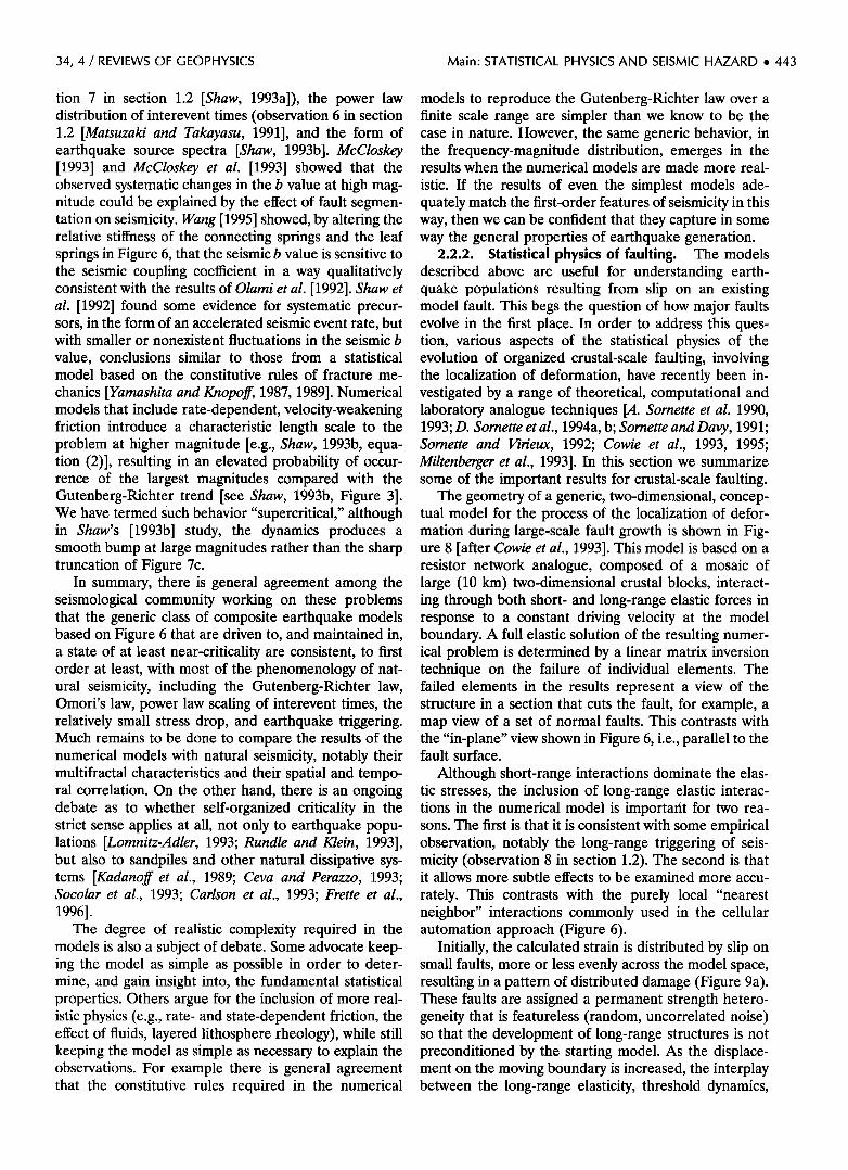
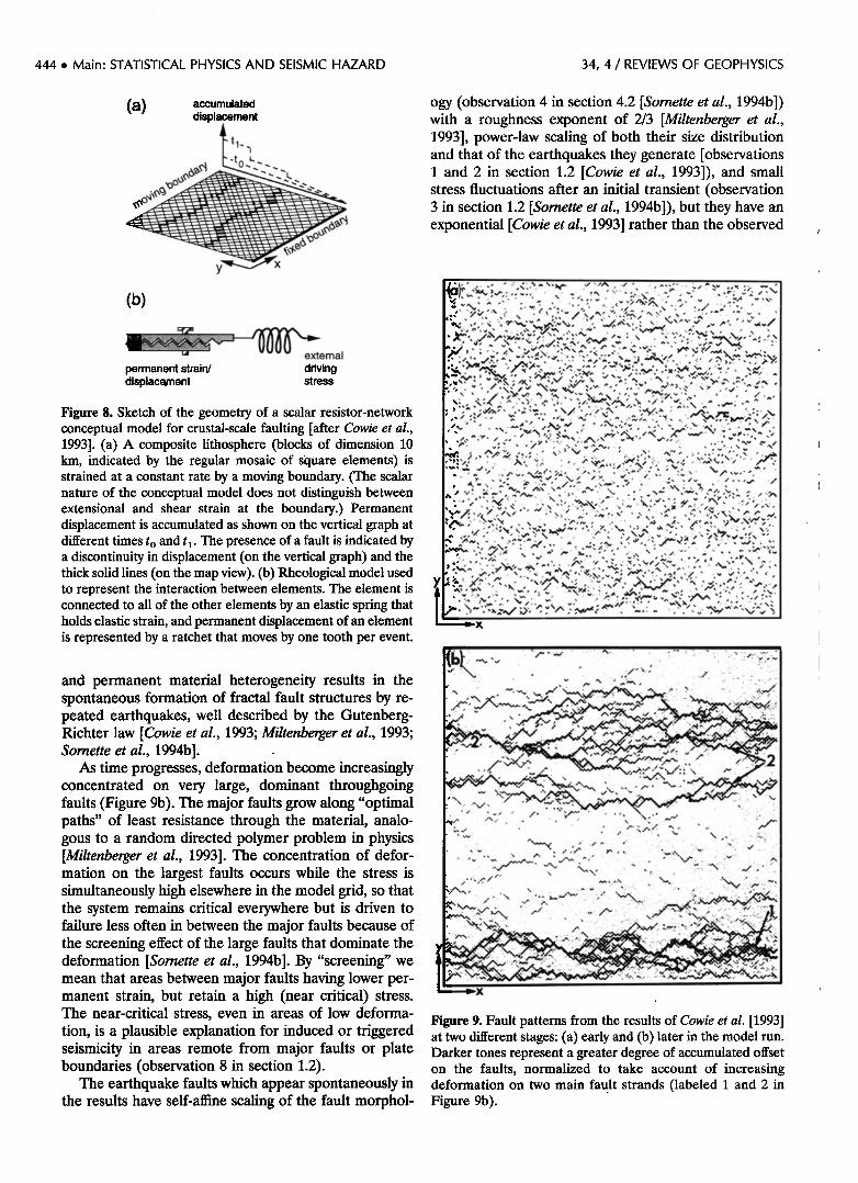
Initially, the calculated strain is distributed by slip on small faults, more or less evenly across the model space, resulting in a pattern of distributed damage (Figure 9a). These faults are assigned a permanent strength hetero- geneity that is featureless (random, uncorrelated noise) so that the development of long-range structures is not preconditioned by the starting model. As the displace- ment on the moving boundary is increased, the interplay between the long-range elasticity, threshold dynamics,
444 ß Main' STATISTICAL PHYSICS AND SEISMIC HAZARD 34, 4 / REVIEWS OF GEOPHYSICS
(a) accumulated displacement
(b)
'•, '-•.•.•••:•:...,•-•-.•":-•U'•-..• Iiii ß external
permanent strain/ driving displace•nent stress
Figure 8. Sketch of the geometry of a scalar resistor-network conceptual model for crustal-scale faulting [after Cowie et al., 1993]. (a) A composite lithosphere (blocks of dimension 10 km, indicated by the regular mosaic of situare elements) is strained at a constant rate by a moving boundary. (The scalar nature of the conceptual model does not distinguish between extensional and shear strain at the boundary.) Permanent displacement is accumulated as shown on the vertical graph at different times t o and t•. The presence of a fault is indicated by a discontinuity in displacement (on the vertical graph) and the thick solid lines (on the map view). (b) Rheological model used to represent the interaction between elements. The element is connected to all of the other elements by an elastic spring that holds elastic strain, and permanent displacement of an element is represented by a ratchet that moves by one tooth per event.
and permanent material heterogeneity results in the spontaneous formation of fractal fault structures by re- peated earthquakes, well described by the Gutenberg- Richter law [Cowie et al., 1993; Miltenberger et al., 1993; Sornette et al., 1994b].
As time progresses, deformation become increasingly concentrated on very large, dominant throughgoing faults (Figure 9b). The major faults grow along "optimal paths" of least resistance through the material, analo- gous to a random directed polymer problem in physics [Miltenberger et al., 1993]. The concentration of defor- mation on the largest faults occurs while the stress is simultaneously high elsewhere in the model grid, so that the system remains critical everywhere but is driven to failure less often in between the major faults because of the screening effect of the large faults that dominate the deformation [Sornette et al., 1994b]. By "screening" we mean that areas between major faults having lower per- manent strain, but retain a high (near critical) stress. The near-critical stress, even in areas of low deforma- tion, is a plausible explanation for induced or triggered seismicity in areas remote from major faults or plate boundaries (observation 8 in section 1.2).
The earthquake faults which appear spontaneously in the results have self-arline scaling of the fault morphol-
ogy (observation 4 in section 4.2 [Sornette et al., 1994b]) with a roughness exponent of 2/3 [Miltenberger et al., 1993], power-law scaling of both their size distribution and that of the earthquakes they generate [observations 1 and 2 in section 1.2 [Cowie et al., 1993]), and small stress fluctuations after an initial transient (observation 3 in section 1.2 [Sornette et al., 1994b]), but they have an exponential [Cowie et al., 1993] rather than the observed
Figure 9. Fault patterns from the results of Cowie et al. [1993] at two different stages: (a) early and (b) later in the model run. Darker tones represent a greater degree of accumulated offset on the faults, normalized to take account of increasing deformation on two main fault strands (labeled 1 and 2 in Figure 9b).

34, 4 / REVIEWS OF GEOPHYSICS Main: STATISTICAL PHYSICS AND SEISMIC HAZARD ß 445
power law temporal correlation in earthquake interevent times (observation 6 in section 1.2 [Turcotte, 1992]).
Cowie et al. [1995] also investigated the multifractal scaling spectrum of higher-order dimensions calculated by weighting the observation of a fault in a box-counting algorithm by the cumulative slip on the fault. The ca- pacity dimension D o is dominated by the initial random distribution of small faults and remains constant at the
Euclidean dimension, 2, of the model space. However, the higher-order dimensions corresponding to higher- order moments of the distribution decrease systemati- cally in the results as the deformation becomes more concentrated. This is accompanied by a decrease in the exponent of the length distribution [Cowie et al., 1995], as seen in analogue experimental data [Davy et al., 1992]. The resulting multifractal spectrum (characterized both by D q and f(ot) discussed above) has a qualitative shape similar to that found for the clustering of natural seis- micity (observation 5 in section 1.2 [Geilikman et al., 1990]). Thus a progressively organized (multifractal) pattern of faulting develops even when the initial heter- ogeneity of rock strength is set to be random, uncorre- lated noise.
The appearance of a multifractal spectrum, indicative of spatial clustering, is also accompanied by systematic changes in the earthquake frequency-magnitude distri- bution. After an initial fault nucleation stage dominated by the correlation length of the background noise, the synthetic earthquake populations progress during the "growth" phase of the faulting through distributions similar to the subcritical to critical examples illustrated in Figures 7a and 7b [Cowie et al., 1993]. Thus the Gutenberg-Richter law emerges as the correlation length in the model results increases to a value near infinity (the largest faults cross the model space).
The spontaneous emergence of large faults is all the more remarkable because no material weakening is in- voked in the numerical model during accumulated slip. The highly organized pattern of faulting is therefore due solely to the statistical physics of elastic-brittle failure, including the effects of long-range elastic interactions, in a heterogeneous granular medium. This provides a plau- sible mechanism for the spontaneous development of large-scale brittle faulting on Earth, even from an ini- tially featureless material heterogeneity on the scale of t0 km or so. This mechanism is important because such organized faulting is a necessary first step to the devel- opment of new plate boundaries. However, Earth has a spatially-correlated geological heterogeneity, even in its early history, so it will be important in future to investi- gate the effects of different geologically realistic initial and boundary conditions on the resulting dynamics.
2.2.•. Fault nucleation. The conceptual model of Figure 8 describes the development of concentrated slip in a preexisting coarse-grained mosaic of faulted blocks of scale length t0 km. In this section we consider how such large faults may grow from even smaller-scale pro- cesses and how controlled laboratory experiments can
help us discriminate between different mechanisms sug- gested for their larger-scale properties. The great advan- tage in laboratory studies is that dynamic variables such as the applied stresses may be measured independently, whereas in the Earth even the reported "stress" mea- surements are essentially scaled from observations of strain [Zoback, 1992]. The great disadvantage is the mismatch of laboratory strain rates (>10 -8 S -I) com- pared with tectonic rates (<t0 -12 s-l), where even the quoted upper bound for natural Earth strain is only seen by monitoring very close to active faults.
One aspect of the nucleation of larger faults from smaller ones is the scaling of displacement u with fault length L. This problem has been studied by various groups, often using combined data sets to attain the necessary bandwidth. Depending on the methods used, different groups have proposed self-similar scaling (u cr L [Cowie and Scholz, t992a]) or a systematic increase in displacement with the larger faults (u cr L 1.5 [Marret and Allmendinger, 1991] or u •c L 2 [Walsh and Watterson, 1988]). Scale-invariant behavior is consistent with an analytic elastic-plastic model developed for postyield fracture mechanics [Cowie and Scholz, t992b], rather than with a purely elastic fault growth model where u cr L ø'5 [Scholz, t990a], or a kinetic model where the fault grows by increments whose size is a constant, irrespec- tive of fault length (u •c L 2 [Walsh and Watterson, 1992]).
The combined data can be interpreted as showing scale invariance in two separate domains of "small" and "large" earthquakes [Cowie and Scholz, t992a], but with a transition to a systematically greater offset at a scale length corresponding to the seismogenic thickness (t0 km or so [Scholz, 1982]). At this characteristic scale the implication is that faults accumulate slip faster than they grow. Thus there is some evidence that the large-scale granularity of the crust, on a scale length of t0 km or so, assumed in the resistor network model described above, is at least plausible.
Cowie et al. [1996] review some of the recent progress in understanding the scaling properties of fault popula- tions. One of the conclusions they come to is that the debate on the precise value of the scaling exponent may be less important than an explanation for the large degree of real scatter in the plots, which gives rise to much of the uncertainty in the interpretations. A similar real scatter can be seen in the dynamic stress drop as a function of earthquake source length in Figure 4 [Aber- crombie, t995], also reflected in the scaling of seismic moment with fault rupture area in the results of the numerical experiments of Gross [1996]. This is testament to the dynamic complexity of the mechanism of fault growth and is likely to be related to the same underlying physics of fluctuations and interactions described above.
One of the problems of interpretations based on composite data sets is the difficulty of combining the data sets objectively. Figure 10 shows an example of a single broadband study of tensile fractures developed in
446 ß Main' STATISTICAL PHYSICS AND SEISMIC HAZARD 34, 4 / REVIEWS OF GEOPHYSICS
2-
• o
a I 2- b
, ,,/" +
4-.
* I + $•*+, -•-
, ! , , , , , , , 0 1 2 3 4 -1
2-
log (length (m))
-1-
o 3 4 -1
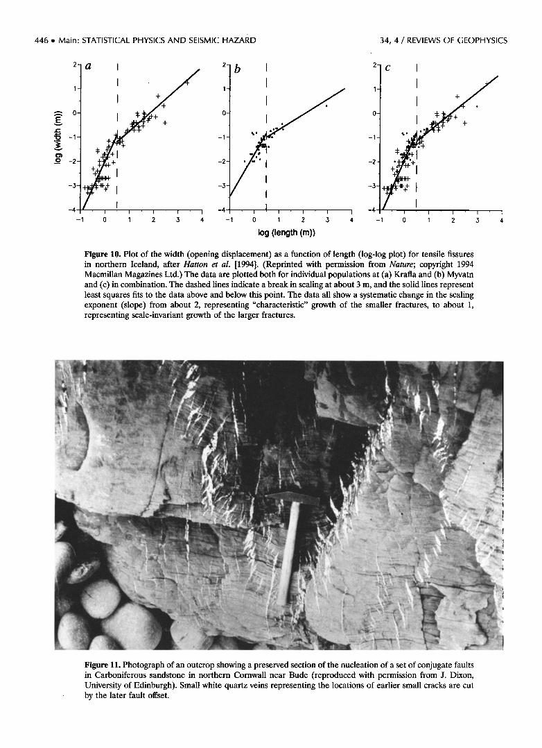
Figure 10. Plot of the width (opening displacement) as a function of length (log-log plot) for tensile fissures in northern Iceland, after Hatton et al. [1994]. (Reprinted with permission from Nature; copyright 1994 Macmillan Magazines Ltd.) The data are plotted both for individual populations at (a) Krafla and (b) Myvatn and (c) in combination. The dashed lines indicate a break in scaling at about 3 m, and the solid lines represent least squares fits to the data above and below this point. The data all show a systematic change in the scaling exponent (slope) from about 2, representing "characteristic" growth of the smaller fractures, to about 1, representing scale-invariant growth of the larger fractures.
...
., .½,&. '.?. ,.. • .:-. .,....-..:,, --.:..:. ........ ;:•:i';;;:•':'•::.;" ' "*;i: , ' ':;'..
::- •,,:.•.
:
%:.:i'
..
.:.
Figure 11. Photograph of an outcrop showing a preserved section of the nucleation of a set of conjugate faults in Carboniferous sandstone in northern Cornwall near Bude (reproduced with permission from J. Dixon, University of Edinburgh). Small white quartz veins representing the locations of earlier small cracks are cut by the later fault offset.

34, 4 / REVIEWS OF GEOPHYSICS Main' STATISTICAL PHYSICS AND SEISMIC HAZARD ß 447
the Krafla and Myvatn fissure swarms in northern Ice- land. The scaling is a power law, but with a marked break of slope from 2 for small fractures (<3 m) to 1 for larger ones. A slope near 2 is consistent with crack growth by a constant increment AL, independent of crack length L, and a slope near 1 is consistent with AL •c L [Hatton et al., 1994]. The material through which these fractures have grown is a homogeneous basalt, with joints on a scale length of the order of 30 cm, so the transition from "characteristic" growth (AL = const) to scale-invariant growth (/XL • L) does not occur pre- cisely at the structural "grain" size provided by the cooling joints. Thus the mechanical grain need not be equivalent to the most evident structural grain. Paradox- ically, such fractal scaling of the structure above this grain size implies a scale-dependent crack extension force, similar to that reported in ceramic materials, possibly as a result of increasing energy demand from a process zone of damage surrounding the crack and con- centrated at the tip [Hatton et al., 1994]. Whatever the explanation, Figure 10 illustrates the general point that scale invariance is always underpinned by granular pro- cesses at smaller scales, also a feature of all of the physical models described above (i.e., the inherently discrete blocks in Figures 6 and 8).
Tensile cracking may also be important in fault nu- cleation at depth, even though the principal tectonic stresses are compressive. An example of an outcrop where an incipient process of fault nucleation has been preserved is shown in Figure 11. Here a small shear offset cuts an organized band of smaller and earlier en-echelon dilatant fractures, now filled with quartz lo- cally derived by pressure solution from the host rock. Dilatant cracking may occur locally under compression, in the presence of fluid overpressure, or strong local stress gradients in a mechanically granular material. However, the growth of a tensile crack is rapidly arrested 'in a compressive stress field, for example, by the mech- anism of dilatant hardening [Scholz, 1990a]. Thus a negative feedback (hardening) process initially results in a distributed array of isolated tensile cracks similar to Figure 9a. The rate constants of fluid flow and mineral precipitation therefore exert .a strong influence on the size and spacing of these arrays of microfractures. Even- tually, the microfractures begin to interact, coalescing to produce a shear fault on a larger scale [Main et al., 1993].
The phenomenon of crack coalescence can be inves- tigated by microseismic techniques in the laboratory. Locknet et al. [1991] used servo-control on the recorded acoustic emissions to slow down the fault nucleation
process in granite specimens and demonstrated conclu- sively that shear faulting is preceded by progressively more localized microcracking along the incipient fault plane. It is this process that has been frozen into the exposure seen on Figure 11. Such crack interaction rep- resents a positive feedback mechanism which may be quasi-static or dynamic, depending on the strain rate and
Zone of Damage
ß ...? ß . ....•.•. , .:.;. :' .t•q•"'...: ..:.. ß :. .(, ,',[.. :'...,. ,;.
:.. . ..•.-'•;.:" ,•. .... :.., ..::• ß .. •....•..,;.
ß .:'•.:-.'•.,.'•::•;:.:.::.::•: .' ....... ß ..,,a•.::,.?' . ß :-"' ,::i...:!'._':;i...'-;i•:'"':' . ..:...::....,¾i.::.:...' ,.. .....',•
•'?.."."'•':"' ' '..."•':;? .•.2:g'-" "' ' ,.•:.."."•:•"": ;' :' ':' ß •:i•'.'•".• ..... :' ' ..,
ß .: ... •fi.•p:.. .. . ß , ..•.: ß
.;:. 5 :': .... ...,:
ß :'"' ' :i•:' . . . :. ...../-- .' .. ..11.-..•i,...,..:
ß .:.:' '- .... '•:r,: ß
!?-??.; .:";:' ,: ; '"'" .. ß •i....":.':;'::'"'";.• ': ' ii•.-;.", .:.':'..':." .... ..":; ?' ;.. :i ..
ß '•: •....; '" .
Intact Rock Fracture 'Process Zone'
Figure 12. A snapshot of failed elements (shown in black) in the results of a cellular automaton model with local rules of
hardening and softening [after Henderson et al., 1994]. White areas represent intact rock, stippled areas represent zones of damage containing isolated microfractures (generated by a hardening rule), and large black areas represent areas where the microcracks have coalesced into a macroscopic fracture (generated by a softening rule). The two rules are combined in a single operator f, which modifies the fracture toughness field K'? -• f327 after the failure of a neighboring element. The form used by Henderson et al. [1994] is f = (1 + pe-(n-4)2/20)e-n2/16, where n is the number of failed neighboring elements and p is an empirical negative feedback or hardening parameter. Large fractures are usually surrounded by a zone of damage similar to a "process zone" seen in ceramics and other composite materials.
the relative physicochemical properties of the fault zone and the surrounding rock.
The cellular automaton approach has also been used to examine the process of fault nucleation by the coales- cence of such dilatant microcracks. For example, Hen- derson et al. [1994] showed that the scale length of local dilatancy has a systematic effect on the seismic b value, by examining the effect of hardening and softening feed- back rules on the form of fracture growth and coales- cence, projected onto the plane of a shear crack [Wilson et al., 1996]. The conceptual models of Henderson et al. [1994] and Wilson et al. [1996] describe a single cycle of quasi-static fracture growth, and do not include healing. Figure 12 shows a snapshot of the evolution of the crack array obtained from the results of Henderson et al. [1994], which show many of the characteristic features of

448 ß Main' STATISTICAL PHYSICS AND SEISMIC HAZARD 34, 4 / REVIEWS OF GEOPHYSICS
15.0
10.0
5.0
0.0 0.0
p--1.0 •=3.0 p:2.0
i
5.0 10.0
magnitude, m
15.0
Figure 13. Equivalent cumulative frequency-magni- tude distribution (log linear plot) for populations of synthetic cracks such as those shown in Figure 12, for different values of the hardening parameter p, also defined in the caption to Figure 12 [after Henderson et al., 1994]. Increasing p implies greater local hard- ening. N is the number of earthquakes with magni- tude greater than m; the magnitude is calculated from the logarithm of the area of clusters of con- nected failed elements similar to Figure 7. The data show three ranges: a characteristic peak at the small- est magnitudes, a scale-invariant range at intermedi- ate magnitudes, and an exponential decay at high magnitudes.
crack growth in the laboratory, including isolated dila- tant cracks, large connected clusters surrounded by a zone of damage (process zone), and large correlated areas with no or relatively little damage. Similar behav- ior is seen when the simple rules of the cellular autom- aton are replaced by a quasi-static solution to the cou- pled problem of deformation and fluid flow, using a lattice gas to simulate the effect of a fluid phase [Wilson et al., 1996]. Wilson et al. [1996] also showed that the geometrical evolution of crack arrays in the results is
sensitive to the initial mechanical heterogeneity, similar to the subcritical class of models of Rundle and Klein
[1993], illustrated in Figure 7a. Crack size distributions obtained by Henderson et al.
[1994] from different snapshots such as Figure 12 are shown in Figure 13. Power law scaling applies only in the middle range of scales. A marked break in slope is seen in the results for cracks smaller than a characteristic
length, determined not by an inherent material grain scale, but by the local mechanical hardening rule. This
Whin Sill Dolerite K I (NN.m -3/2) 'b' 3 1 2.97- 3-05 1.38
2 2.82- 2.87 1.60
3 2. t.1- 2.60 1.82
2.20- 2.'31 2-00 2-11- 2.19 2.86
S t. 3 2 1 I I I I I I
0 20 t.o 60
Amplitude (dB}
H20 liquid 20øC ß o granite
I I I I I I I 80 100 0 0.2 0-4 0'6 0'8
K/K c 10
Figure 14. (left) Cumulative frequency-amplitude distributions for acoustic emissions during the quasi-static tensile failure of notched double torsion samples of Whin Sill dolerite in water at 20øC (after Meredith et al. [1990]; reprinted with kind permission of Elsevier Science-NL, Sara Burgerhartstraat 25, 1055 KV Amster- dam, Netherlands). The different distributions 1-5 correspond to different stress intensity factors (K/) and b values measured during different stages of a single test run. (The test runs are controlled by gradually increasing the stress intensity, so the quoted values for K/are listed as ranges rather than single figures). (right) A composite plot of measured b value and stress intensity factor for test runs on different crystalline rock types and water saturation. For these tests the constant c (equation (5)) is equal to 1, so the exponent of the source length distribution, D, is equal to b [Meredith et al., 1990]. The stress intensity factor is normalized by the fracture toughness Kc to allow direct comparison of the different tests. Solid lines represent least squares fits through the resulting composite data, showing a systematic difference between nominally water-saturated ("wet") and air-dried ("dry") samples, which decreases as the stress intensity increases.
ITI

34, 4 / REVIEWS OF GEOPHYSICS Main' STATISTICAL PHYSICS AND SEISMIC HAZARD ß 449
1,5
b ' ' ' 5 . , , '1.0
1.o 3
05 • ,111• I I , , I I. 1 .I. ! , ......
0.5
0.0 0.0 50.0 100.0 150.0 200.0
Remote stress
Figure 15. Evolution of the seismic b value with time (represented by increasing applied stress) from the results of Henderson et al. [1994], with different values of the hardening parameter p. The b values determined by Henderson et al. [1994], based solely on the mean magnitude of the whole data range, have been rescaled for the intermediate range of data shown in Figure 13 [see Main et al., 1994]. The inset shows the behavior (including typical error bars) observed in field-scale investigations of earthquake sequences (redrafted with permission from Nature [after Smith, 1981]; copyright 1991 Macmillan Magazines Ltd.). The vertical lines in the inset correspond to individual large events (with their magnitude scale given on the right-hand side).
illustrates the concept of a local mechanical "grain" from the physical process, also required to explain the break in slope of the data in Figure 11 [Hatton et al., 1994]. The biggest cracks in the model snapshots have not yet crossed the entire grid, so a subcritical (compare Figure 7a) size distribution results at larger scales. The results also show a systematic increase in b value, asso- ciated with a smaller maximum magnitude, as the degree of negative feedback or hardening increases. This is similar to the behavior seen in the nonconservative
spring-block-slider model of Olami et al. [1992] and in the scaling of seismicity induced by hydraulic mining [Main et al., 1994].
A positive correlation of increased negative feedback with decreased b value is also seen in laboratory exper- iments during quasi-static crack growth by stress corro- sion (Figure 14 [after Meredith et al., 1990]). The impor- tant controlling variable in the results of Meredith et al. [1990] is the stress intensity (proportional to the square root of the crack extension force), a measure of the concentration of elastic stress at the crack tip. At low stress intensities, energy, which may have been available to drive the main crack, is dissipated in local physico- chemical fluid-rock reactions that produce a zone of
damage (process zone), which screens the main crack from the remote stress, similar to that seen in Figure 12.
The results of several similar experiments on different crystalline rock types are also shown in Figure 14, which plots the b value as a function of the normalized stress intensity (K/Kc) , where K c is the fracture toughness of the rock type used. The normalized stress intensity and the presence of fluids both have systematic first-order effects on the b value in these tests on initially intact rock. Stress intensity increases in proportion to both the applied stress and the square root of the crack length, so fracture growth itself increases the stress intensity, which in turn feeds back into faster crack growth. Such non- linear, local, physics is just one example of how an accelerating or avalanche-type process can develop through local feedback rules.
In a true state of self-organized criticality we might expect the b value to remain unchanged or to change only slowly in comparison with the event rate [e.g., Shaw et al., 1992]. The predicted evolution of the seismic b value in the numerical model of Henderson et al. [1994] is shown in Figure 15. For zero negative feedback (p = 0) the b value decreases monotonically, and failure is ap- proached rapidly because of the absence of local hard-

450 ß Main- STATISTICAL PHYSICS AND SEISMIC HAZARD 34, 4 / REVIEWS OF GEOPHYSICS
u,,,, / s•,u•^• :IV 0 0 0 0 0 0 o o o o o o o o o o o o
anloA-q
0 0 0 0 0 u• 0 ½'4 •- •- • 0
0 ] [ • [ ] [ I I [ I [ [ I ! [ I I I I I • I I I ' [ I I • I O
• O ß
• . _
.
o 8••
I', ......... , ......... , ......... , ........ •'•;; o
> (Odl//) aJnssaJd Pinl-I aJOd
u,w / s•,ua^a :IV anloA-q
lllilllll]l]1111 o • • •

34, 4 / REVIEWS OF GEOPHYSICS Main: STATISTICAL PHYSICS AND SEISMIC HAZARD ß 451
ening. This behavior is similar to 'that seen in the results of Huang and Turcotte [1988]. However, for finite nega- tive feedback (p > 0), failure is delayed, and a temporary increase followed by a shorter decrease in b value is seen, similar to some reported observations of natural seismicity (see inset [after Smith 1981]). The results of Henderson et al. [1994], although near-critical, do not exhibit the insensitivity to local dynamics of strict self- organized criticality.
Similar fluctuations in b value, associated with de- layed failure, are seen in controlled laboratory experi- ments during fault nucleation (Figure 16 [after Sam- monds et al., 1992]). In these tests, experiments done under "drained" conditions (where dilatancy hardening cannot occur, so p = 0) show a constant pore pressure and a monotonic decrease in b value. However under
"undrained" conditions the pore fluid pressure drops, implying local dilatancy hardening according to Figure 12 (p > 0). The effects of such local negative feedback on the fracture process are both to delay failure and to introduce a temporary increase and then a decrease in the seismic b value. These qualitative features are also seen in the results shown in Figure 15. In contrast, the presence of a fault is marked by a relatively constant b value in the period of stable sliding (Figure 16). A relatively constant b value during stable sliding is also seen in the experimental results of Meredith et al. [1990] and Locknet et al. [1991].
Thus fault nucleation, although it does produce power law scaling, is not an example of true self-orga- nized criticality because the b value depends strongly on the external variables (notably stress intensity and pore pressure). Instead, fault nucleation is more consistent with the subcritical class of models illustrated in Figure 7a, implying a strong sensitivity to material heterogene- ity, external forcing, and the effective dissipation in the form of fluid-rock interactions. However, once a fault is present, the b value remains relatively constant [Meredith et al., 1990; Locknet et al., 1991; Sammonds et al., 1992; Liakopoulou-Morris et al., 1994].
The main outstanding question in fault nucleation concerns the precise nature of the underlying character- istic granularity of the brittle crest: is this the mineral grain of the rocks (millimeter scale), or is it due to some mechanical grain associated for example with local dila- tancy hardening, or some other process, at a greater length scale? The smallest natural earthquakes for which stress drops have been inverted from a sufficiently broad band of data [Abercrombie and Leafy, 1993; Abercrombie and Brune, 1994; Abercrombie, 1995] show scale invari- ance in stress drop and b value down to a source length of 10 m or so. Therefore this granularity may lie some- where between the mineral grain (millimeters) and 10 m, equivalent to the lower scale range of field studies shown in Figures 4 and 11. It is evident that more detailed work is required in the sub-10-m scale range, both at outcrop and in settings where such small-scale seismic events can be recorded (e.g., in mines and hydrocarbon fields).
3. APPLICATION TO SEISMIC HAZARD
So far we have concentrated on the fundamental
problems of how to explain the phenomenology of earth- quakes and seismogenic faulting in the Earth on a broad range of scales. In this section we now consider the implications of a state at or near self-organized critical- ityma state bordering on deterministic chaos--for the practical problems of earthquake prediction and seismic hazard estimation.
3.1. Earthquake Prediction? We have already addressed some of the problems
associated with identifying earthquake precursors in the introduction. Although no precursors satisfying all of the criteria cited by Wyss [1991, box 3] have been found, three were accepted onto a "preliminary list of signifi- cant earthquake precursors" [Wyss, 1991, p. 1], as fol- lows: (1) seismic quiescence before strong aftershocks (many cases); (2) foreshocks (February 4, 1975, M = 7.3 Haicheng earthquake); (3) radon concentration de- crease (January 14, 1978, M = 7.0 Izu-Oshima-Kinkai earthquake). This list does not imply that these are definite precursors, merely that "the majority of review- ers and panelists thought it more likely than not that the method might be useful for earthquake prediction" [Wyss, 1991, p. 1]. If we assume that the initial sample of 28 precursors submitted to this exercise is already pre- selected by those taking part to be the "best examples," then the whole question of the general existence of precursors is called into question on empirical grounds. We have also seen'that reliable prediction may not even be possible in principle, owing to a combination of (1) nonlinear dynamics, involving triggering or avalanche- type processes [e.g., Brune, 1979; Bak and Tang, 1989]; (2) incomplete or imperfect data sampling [e.g., Scholz, 1990a; Wyss, 1991]; and (3) a system existing in a per- petual state of marginal stability, where physical fluctu- ations resulting in apparent statistical "noise" are inher- ent to the process [Bak et al., 1988a; Rundle, 1988].
On the optimistic side, Keilis-Borok [1990], in a review of the implications of a conceptual model of the litho- sphere of the Earth as a nonlinear system, concludes that earthquake prediction may at least be possible despite the aforementioned problems. On the other hand, Geller [1991, 1996] points out that there is no consensus among seismologists on whether earthquake prediction is pos- sible, even in principle, and argues that seismologists should instead concentrate their efforts more on achiev-
ing a better understanding of seismogenesis as a process. In a recent concrete example, Abercrombie and Mori [1996] have shown that there is no systematic relation- ship between tiny aspect of foreshock occurrence and the magnitude of the subsequent mainshock in the western United States. Similarly, Mori and Kanamori [1996] ex- amined the nature of precursory seismic radiation im- mediately (i.e., seconds or fractions of a second) prior to the main energy release in a range of earthquakes of

452 ß Main- STATISTICAL PHYSICS AND SEISMIC HAZARD 34, 4 / REVIEWS OF GEOPHYSICS
different sizes in the 1995 Ridgecrest, California, se- quence and concluded that the size of the nucleation zone for the precursory seismic radiation was of the order of 10 m or less, independent of the eventual size of the mainshock. They conclude that the size of the earth- quake is determined by the nature of rupture arrest, rather than the nucleation process, consistent with the notion of earthquake triggering and avalanche dynamics. Thus at least one of the crucial elements of a successful
earthquake prediction (i.e., the magnitude), cannot, at least yet, be made from short-term precursory data cru- cial to the triggering process (foreshocks or immediate seismic precursors). This problem is potentially even more severe for intermediate-term precursors.
In the meantime the numerical models that have been
developed to explain seismogenesis as a critical phenom- enon may be used at least to assess the likelihood of prediction in an ideal case where our knowledge is complete. That is, if we cannot predict synthetic earth- quakes in a computational system, which is deterministic but simplified, we may be forced to conclude that inter- mediate-term prediction in the Earth, with incomplete data sampling and more complicated physics, may be inherently unattainable. In this vein, Shaw et al. [1992] observe some premonitory intermediate-term and short- term changes in seismicity rate and pattern in the results of their version of the Burridge-Knopoff model. More recently, Pepke et al. [1994] found that the heuristic pattern-recognition algorithms developed by trial and error from real earthquake sequences [Keilis-Borok and Gossubov, 1990; Keilis-Borok et al., 1990] can be applied successfully to a dynamic model of a fault, at least for the case of a cycle involving the failure of the entire model space in a single dynamic event. By comparing theoret- ical results from numerical models, run with different starting assumptions, parameters, and boundary condi- tions, with observations, we may iterate to a better understanding of the physical basis for precursors. How- ever, the true test of reliable earthquake prediction as a practical proposition will remain with the statistical ex- amination of real (and noisy) discrete data.
In summary, some preliminary modeling work on the dynamic complexity of earthquake populations shows that we cannot yet reject the theoretical possibility of the predictability of location, time, and size of individual earthquakes in model earthquake sequences, at least under certain conditions [e.g., Shaw et al., 1992]. How- ever, physically realistic solutions in similar dynamical models can also be obtained with no precursors, consis- tent with recent observations of earthquake triggering. In terms of real data, there is still no conclusive proof that earthquake precursors, at least as defined by Wyss [1991], do exist generally in nature. Thus despite over 100 years of effort, we seem to be moving no closer to having a useful earthquake prediction capability [Geller, 1996], although work is continuing in this area. In con- trast, jhe implications for a probabilistic seismic hazard analysis based on a population of earthquakes may be
much more important and i•mediately useful but have received much less attention to date. We consider this
application in the following section.
3.2. Seismic Hazard
Earthquakes are a significant natural hazard that an- nually bring disaster to a significant and growing number of the world's population, predominantly in areas near plate boundaries (e.g., the great Michoacan earthquake of September 19, 1985, Ms - 8.1 [Press et al., 1987, p. 5]. However seismic risk can also be significant far from plate boundaries, as is illustrated by the recent Khillari earthquake in central India on September 29, 1993 (M s = 6.3), which claimed many thousands of lives, partly because of the low seismic attenuation in cratonic litho-
sphere but also owing to a perception of low hazard and limitations on affordable local building practices. In fact, all three recorded earthquakes causing the largest loss of human life occurred in an intraplate setting (China, 1556, 1920, and 1976). Many other examples could be cited here.
The seismic risk therefore depends both on the seis- mic hazard (source, path, and local site conditions) and on engineering and social conditions such as the vulner- ability of individual buildings, the population affected, and the actual or achievable level of preparedness. The background seismic hazard, which ultimately depends on the dynamics and structure of the solid planet, is a proper study for Earth scientists. Economic and engi- neering decisions are also based on a vulnerability which is steadily increasing as more and more cities with larger populations are built in earthquake-prone areas [Reiter, 1991]. For example it is estimated that 290 million "su- percity" dwellers, 80% of them in developing nations, will live in a region of significant seismic risk by the end of the millennium [Bilham, 1988].
Although the seismic risk is increasing, the seismic hazard remains relatively constant (at least when aver- aged over long time periods) because of the relative stability of global dynamics through the extremely linear and predictable phenomenon of surface plate tectonics. The regularity of plate tectonics exists when a dynamic equilibrium of driving forces, striving to lose heat from the mantle, is achieved with a constant terminal velocity in the individual fragments of a rigid outer shell (the lithosphere). For example, the current pattern of mantle heterogeneity, based on seismic tomography and obser- vations of the geoid, is reasonably well matched by plate tectonic reconstructions of subduction extrapolated back over the last 120 m.y. [Richards and Engebretson, 1992]. On shorter (decadal) timescales the results of global satellite geodesy have also shown a marked linear con- sistency with the same plate model [DeMets, 1995]. This stationarity is reassuring because since its inception, the concept of plate tectonics has had a great impact on the calculation of seismic hazard through seismotectonic considerations [Lomnitz, 1974].
However, plate tectonics cannot always be used sim-

34, 4 / REVIEWS OF GEOPHYSICS Main: STATISTICAL PHYSICS AND SEISMIC HAZARD ß 453
ply to predict seismic hazard. For example, although there is a close association of earthquakes with plate boundaries, we have seen that damaging earthquakes may occur virtually anywhere. Thus although the seismic hazard tends to be higher at the edges of plates, it is not zero elsewhere because plates are not completely rigid elastic bodies. In particular, continental deformation often involves significant stretching or shortening of the lithosphere, and the pattern of shallow seismicity is often more diffuse in back-arc provinces in such regions. Nev- ertheless, the first-order pattern of seismicity and focal mechanisms is in good agreement with the first-order features of global tectonics [e.g., Lomnitz, 1974].
A stationary state of self-organized criticality, or at least a stationary state maintained near criticality as discussed above, gives a good rationale for predicting the future hazard on the basis of past occurrence, a basic tenet of all current practices in seismic hazard estima- tion [e.g., Reiter, 1991]. Although the dynamic release of stored elastic energy in individual events may be inter- mittent and unpredictable, the average strain energy release in the earthquake population as a whole would be expected to remain constant over long timescales. This single result removes much of the uncertainty in- volved in seismic hazard estimation, using what has, up to now, been an a priori assumption of "stationarity" in the earthquake process. However, the underlying me- chanics predicts significant dynamic fluctuations about this metastable state, so the application of this assump- tion depends critically on having a long enough statisti- cal sample compared with the recurrence rates of the largest events. If short-term dynamic fluctuations are an inevitable consequence of the underlying physics, then we should likewise adopt a conservative approach to seismic hazard estimation.
A second key assumption in much seismic hazard analysis is that earthquakes are a random Poisson pro- cess [e.g., Reiter, 1991]. However, the strongly interacting nature of avalanche-type dynamics is fundamentally in- consistent with earthquakes as a Poisson process. For example, Brown et al. [1991] applied the Burridge- Knopoff model, with its strong local interactions (Figure 6), to the problem of earthquake recurrence times and their statistical variability. The results show a lognormal distribution of recurrence times that is quantitatively inconsistent with a Poisson process. Lomnitz [1996], by examining the correlation of events in the global seismic moment catalogue of Pacheco and Sykes [1992], con- cluded that even the largest shallow earthquakes occur- ring this century (of moment magnitude M•v > 7.0), may not be independent on timescales less than 1 month for length scales up to several hundred kilometers.
How can we use the long-term metastability of a state near self-organized criticality to combine tectonic esti- mates of seismic slip with earthquake magnitude cata- logues to obtain better estimates of future hazard? One answer is to use the approach of information theory [Shen and Manshina, 1983; Main and Burton, 1984,
1986], where we seek a maximum entropy solution to the available constraints of mean catalogue magnitude (available since about 1900) and mean seismic moment flux (potentially over millions of years). The answer has the form of a modified gamma distribution in the cumu- lative frequency of occurrence:
ax N(Mo) = Nr M;-a-le-•ø' dM;. (4)
Nr is the total number of seismic events in the magni- tude catalogue per unit time; B and X are the distribu- tion parameters, to be calculated from the mean cata- logue magnitude (m) and the mean moment (Me) =
ß ß
Me/Nr, where Me is the measured seismic moment release rate; and M• ax is the maximum seismic moment.
The static seismic moment Me for an individual event is the product of the fault area A, the average displace- ment u, and the shear modulus of the upper crust (ix • 30 GPa) and is related to the magnitude m (ML or Ms) by
log M0 = cm + d, (5)
where c and d are scaling constants. The empirical relation (5) is consistent with a simple dislocation model for the seismic source, where c depends on the relative frequency content of the seismic event and the passband of the recording instrument, and d depends on the mean stress drop [Kanamori and Anderson, 1975; Hanks and Kanamori, 1979]. The dislocation model predicts that for a seismometer response flat to velocity in the typical frequency range of the source spectrum c = 3/2, and for a stress drop of about 3 MPa (30 bars), d = 9.1 (for Me in newton meters). The scaling constant c determines the relationship between the seismic b value and the exponents B (equation (4)) or D (equation (1)). Usually, c - 3/2, so D - 2b and B = 2b/3 [King, 1983; Main and Burton, 1984; Turcotte, 1992].
By adopting this procedure, the long-term seismic hazard can be constrained by a long-term seismic mo- ment release rate 3;/o, determined from paleoseismic, geodetic, or plate tectonic studies and synthesized into a single distribution with the shorter-term seismicity cata- logue via the mean magnitude and the seismic event rate
.
N r [Main and Burton, 1984, 1986]. Implicit in this pro- cedure is the assumption of stationarity in the flux of energy or moment, also present in the mean field statis- tical mechanical model of Sornette and Sornette [1989].
The gamma distribution exhibits power law scaling of energy at small magnitudes, consistent with the term b in equation (2), or B in equation (4), but with a tail at high magnitudes that may either continue this trend right up to the maximum magnitude (X = 0), have an exponential tail (• > 0), or lead to a "characteristic" peak near the largest magnitude (• < 0). This generic behavior is similar to the subcritical (X > 0); critical (X = 0) and supercritical (X < 0) classes of behavior in Figures 7a,
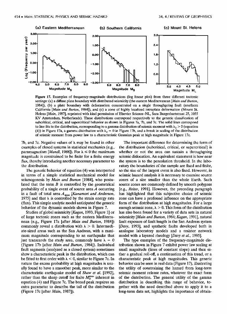
454 ß Main' STATISTICAL PHYSICS AND SEISMIC HAZARD 34, 4 / REVIEWS OF GEOPHYSICS
(a) Eastern Mediterranean
3.00,
2.00.
1.00
0-00•
- 1.00-
-2.00 4.0 9.0 5•0 6•0 7•0 8•0
Magnitude M s
•.00,
1.00
"001 - 1.001 -2-001 -3.OOl
(b) Southern California
5.0 6.0 7.0 8.0
Magnitude M s
(c) Mount St. Helens
3.0
2.4
1.8
1.2
0.6
0 ,
, i I
3.5 4.0 4.5 5.0
Magnitude M L
Figure 17. Examples of frequency-magnitude distributions (log linear plot) from three different tectonic settings: (a) a diffuse plate boundary with distributed seismicity (the eastern Mediterranean [Main and Burton, 1984]), (b) a plate boundary with deformation concentrated on a single throughgoing fault (southern California [Main and Burton, 1984]), and (c) a zone of highly localized intraplate deformation (Mount St. Helens [Main, 1987], reprinted with kind permission of Elsevier Science-NL, Sara Burgerhartstraat 25, 1055 KV Amsterdam, Netherlands). These distributions correspond respectively to the generic classification of subcritical, critical, and supercritical behavior as shown in Figures 7a, 7b, and 7c. The solid lines correspond to line fits to the distribution, corresponding to a gamma distribution of seismic moment with X2 > 0 (equation (4)) in Figure 17a, a gamma distribution with X2 = 0 in Figure 17b, and a break in scaling of the distribution of seismic moment from power law to a characteristic Gaussian peak at high magnitude in Figure 17c.
7b, and 7c. Negative values of X may be found in other examples of closed systems in statistical mechanics (e.g., paramagnetism [Mandl, 1988]). For X -< 0 the maximum magnitude is constrained to be finite for a finite energy flux, thereby introducing another necessary parameter to the distribution.
The generic behavior of equation (4) was interpreted in terms of a simple statistical mechanical model for seismogenesis by Main and Burton [1984], who postu- lated that the term B is controlled by the geometrical probability of a single event of source area A occurring in a fault of total area Ama x [Kanamori and Anderson, 1975] and that X is controlled by the strain energy rate (flux). This simple analytic model anticipated the generic behavior of the dynamic models shown in Figure 7.
Studies of global seismicity [Kagan, 1993, Figure 1] or of large tectonic zones such as the eastern Mediterra- nean (e.g., Figure 17a [after Main and Burton, 1984]) commonly reveal a distribution with X > 0. Intermedi- ate-sized areas such as the San Andreas, with a maxi- mum magnitude corresponding to an earthquake that just transcends the study area, commonly have X = 0 (Figure 17b [after Main and Burton, 1984]). Individual fault segments (analyzed as a closed system) sometimes show a characteristic peak in the distribution, which can be fitted to first order with X < 0, similar to Figure 7c. In nature the excess probability at high magnitudes is usu- ally found to have a smoother peak, more similar to the characteristic earthquake model of Shaw et al. [1992], rather than the sharp cutoff for finite M•0 ax inherent in equation (4) and Figure 7c. The broad peak requires an extra parameter to describe the tail of the distribution (Figure 17c [after Main, 1987]).
The important difference for determining the form of the distribution (subcritical, critical, or supercritical) is whether or not the area can sustain a throughgoing seismic dislocation. An equivalent statement is how near the system is to the percolation threshold. In the labo- ratory the boundaries of the sample are fixed and finite, so the size of the largest event is also fixed. However, in seismic hazard analysis it is necessary to examine source zones of a size smaller than the whole Earth. Such
source zones are commonly defined by smooth polygons [e.g., Reiter, 1991]. However, the preceding paragraph has highlighted that this subjective choice of seismic zone can have a profound influence on the appropriate form of the distribution at high magnitudes. For a large enough seismic zone, X > 0. This form of the distribution has also been found for a variety of data sets in natural seismicity [Main and Burton, 1984; Kagan, 1991], natural fault exposure of fault length in the San Andreas system [Davy, 1993], and synthetic faults developed both in analogue laboratory models and a resistor network model with a layered rheology [Davy et al., 1995].
The type examples of the frequency-magnitude dis- tribution shown in Figure 7 exhibit power law scaling at small magnitude (lines of constant slope) and then ei- ther a gradual roll-off, a continuation of this trend, or a characteristic peak at high magnitudes. This generic behavior can be seen in real data (Figure 17), illustrating the utility of constraining the hazard from long-term seismic moment release rates, whatever the exact form of the distribution. The general utility of the gamma distribution in describing this range of behavior, to- gether with the need described above to apply it to a long-term data set, highlights the importance of obtain-

34, 4 / REVIEWS OF GEOPHYSICS Main: STATISTICAL PHYSICS AND SEISMIC HAZARD ß 455
ing reliable paleoseismic data from suitable trench sites to constrain the long-term slip or recurrence rate of the rare largest earthquakes [e.g., Sieh, 1978; Sieh et al., 1989; Pantosti and Yeats, 1993].
The gamma distribution may also be used to predict the maximum magnitude in seismic hazard analysis [Main, 1995]. A strict maximum magnitude is an essen- tial requirement to avoid infinite energy release pre- dicted by linear extrapolation of the Gutenberg-Richter law [e.g., Reiter, 1991]. However, this introduces a rather unrealistic sharp truncation to the distribution for X -< 0 that is atypical of natural dissipative systems [Kagan, 1993]. In contrast, the gamma distribution (with X > 0) has an exponential tail that is more gradual, so that an effective maximum magnitude can be determined inde- pendently, in terms of a vanishing contribution either to the integrated seismic moment release or to the inte- grated level of ground motion. Although these precise values may be different in general, the maximum mag- nitudes predicted by convolution with the scaling of seismic moment or ground motion attenuation are found to be remarkably similar [Main, 1995].
Our new understanding of the statistical physics of earthquakes also has profound implications for other aspects of seismic hazard estimation. For example, it is evident that the common practice of applying regular seismic zones with smooth Euclidean boundaries to a
potentially multifractal distribution of epicentres may fundamentally precondition the results. Seismic zoning is known to be rather subjective and is notoriously de- pendent on the prejudices of the "expert" used [Krinitzsky, 1993a]. One possible reason is the multifrac- tal nature of seismicity and faulting.
The results described here also suggest that the rather subjective choice of area may also have a systematic effect on the form of the appropriate frequency-magni- tude distribution, with larger areas being more likely to have a subcritical form (Figure 17a). In particular, very local studies concentrated on individual faults are more
likely to produce supercritical or apparently "character- istic" distributions such as Figure 17c. Kagan [1993] has criticized the application of the characteristic earth- quake model (in the sense of a peak in the discrete frequency-magnitude distribution) to instrumental earthquake catalogues on statistical grounds, but Lom- nitz-Adler [1988] and Ward [1992] have argued in its favor on the basis of historical data in the middle Amer-
ica trench. On more practical grounds, Krinitzsky [1993b] has also criticized the apparent "dysfunctionality" of assuming a priori a Gutenberg-Richter law in very small seismogenic zones. In some respects this argument will not be resolved until we have good, homogeneous, in- strumental data for a long enough time to test these models objectively. In the meantime it seems sensible to make the best use of all forms of data covering periods longer than the 100 years or so of instrumental recording.
The general procedure followed in probabilistic seis- mic hazard analysis includes the individual steps of seis-
ß
Magnitude M
Step I Step 2 SOURCES RECURRENCE
Uncertainty o c ß in Attenuation
• ' ß. '.Magnitude M 1
.,
Distance 0 Acceleration
Step 3 Step 4 GROUND MOTION PROBABILITY OF
EXCEEDANCE
Figure 18. Schematic plot of the different stages in probabilistic seismic hazard analysis. (Redrafted after Reiter [1991]. Copy- right 1991 by Columbia University Press. Reprinted with per- mission of the publisher.) Step 1 involves estimating sources represented as smooth objects (lines or areas enclosed in regular polygons). Step 2 involves estimating the recurrence statistics from frequency-magnitude data. Step 3 involves esti- mating the ground motion as a function of source magnitude and distance, often from very scattered data, so that an esti- mate of uncertainty is useful. Step 4 involves the convolution of steps 1-3 to predict the likelihood of exceedance of a given level of ground motion per unit time.
mic zoning, estimating the recurrence, and fitting a local attenuation law to the ground motion in order to calcu- late an annual probability of exceedance of a particular level of ground motion (Figure 18 [after Reiter, 1991]). Our new understanding of the statistical physics of earthquake populations suggests that procedures involv- ing the first two steps, at least, need to be reevaluated.
In summary, our new understanding of the statistical physics of earthquakes has profound implications for some critical steps in the chain of probabilistic seismic hazard analysis, and these are only just beginning to be explored. Many of the problems identified, such as the a priori assumption of the Gutenberg-Richter law or the vagaries of seismic zoning, had already been identified on phenomenological grounds by practitioners in the field [Reiter, 1991; Krinitzsky, 1993a, b], but our new understanding of seismogenesis as a critical phenome- non gives a firmer scientific basis for these conclusions. Perhaps the most important results are as follows: (1) a

456 ß Main: STATISTICAL PHYSICS AND SEISMIC HAZARD 34, 4 / REVIEWS OF GEOPHYSICS
plausible scientific justification now exists for the funda- mental assumption of stationarity in the earthquake process; (2) earthquakes are most likely the result of an avalanche rather than a completely random Poisson process, and (3) we have the means to constrain the hazard and the maximum credible magnitude using a more general equation (equation (4)) than the Guten- berg-Richter law. Perhaps the most important outstand- ing questions raised by the discussion here are (1) what alternatives might there be to regular seismic zoning that truly encapsulate the multifractal nature of seismic sources, and (2) what practical alternatives might there be to the almost ubiquitous assumption of Poisson be- havior in calculating the seismic hazard?
4. DISCUSSION
In this article we have concentrated on evaluating the results of physical models that assume brittle fracture or dynamic friction as a nucleation mechanism for seismic slip. This is appropriate for the shallow earthquakes that dominate the seismic hazard, and may also be extended to intermediate depth earthquakes by pore-pressure- induced faulting due to dewatering of subduction slabs [Thompson, 1992]. However, events deeper than about 350 km may be triggered instead by dynamic instabilities associated with volumetric phase changes in the upper mantle [Green et al., 1992]. Much remains to be done to determine the underlying dynamics of deep earthquakes before we can address their properties in terms of sta- tistical physics. This is important because there seem to be systematic differences in the statistical properties of shallow, intermediate, and deep earthquakes, notably the presence or absence of aftershocks, differences in the scaling of the spatial correlation dimension [Kagan and Knopoff, 1980], and systematic changes in the frequency- moment distribution (i.e., in the parameters B and h of equation (4) [Kagan, 1991]).
We have also not addressed the controversial ques- tion of changes in scaling caused by the finite width of the brittle seismogenic layer [Romanowicz, 1992; Schoh, 1994], partly because the data are not yet able to resolve whether this break is sharp (as these authors suggest) or more gradual (e.g., consistent with the gamma distribu- tion [Main, 1992b; Somette et al., 1996]), This is impor- tant because the different types of changes in scaling for large earthquakes have markedly different implications for seismic hazard evaluation. For example, extrapola- tions based on an apparent increase in b value at high magnitudes (h > 0) have a lower seismic hazard than those with decreasing b value (h < 1 [Marret, 1994]). Kagan [1993] argues that in the absence of conclusive evidence to the contrary, we should adopt the simplest distribution with a statistically satisfactory approxima- tion of the data, namely, the gamma distribution with positive X.
The universality of Figures 7 and 17 is at once reas-
suring and disquieting. It is reassuring because we can now apply these distributions to earthquake data with more confidence, using the techniques described above. This is vital for seismic hazard purposes. However, as we have seen, precisely the same forms of the distribution appear in the results of a wide variety of different nu- merical models with different specific dynamics. There- fore we cannot use these statistical properties alone to invert for the details of the dynamics from real data. Composite dynamic models will therefore continue to be used predominantly in a forward modeling capacity, in particular to look for other aspects that could be used to discriminate for the appropriate local physics.
However, it is important to realize that the study of complexity in seismogenesis is only in its infancy. To date, we have seen that realistic complexity has been introduced at the expense of simplifying the local phys- ical rules to an unrealistic degree. As computers increase in power, we may be able to look at more realistic rheologies (in particular, to examine time-dependent processes and state-dependent friction, and to include long-range interactions more routinely) by replacing the local "rules" of cellular automata with more sound phys- ical equations that have a wider range of applicability. In particular the role of fluids and body forces such as gravity are only beginning to be to be explored in detail [e.g., Rice, 1992; Segall and Rice, 1995; Miller et al., 1996; Matthai and Fisher, 1996], and only a few conceptual models [e.g., Rice, 1993; Ben-Zion et al., 1993; Davy et al., 1995] explicitly include coupling to a more ductile sub- strate. An important unresolved question is the nature of the inherent granularity of the brittle crust: are we dealing with an "inherently discrete" system, as is sug- gested by the discussion in section 2.2.2 on fault nucle- ation, or is there a continuum limit to the mechanics [Rice, 1993]?
5. CONCLUSION
Recent statistical physics models of fault nucleation, fault growth, and seismogenesis as critical (or self-orga- nized critical) phenomena provide a plausible quantita- tive basis for many of the observed scaling properties of earthquakes and fault populations. In this conceptual model, the brittle part of the Earth's lithosphere first evolves spontaneously to a critical or near-critical state and then remains there, apart from discrete fluctuations represented by individual earthquakes. The brittle crust is therefore maintained over long timescales in a station- ary but metastable state of long-term balance between continuous tectonic energy supply and intermittent de- mand from earthquakes. In this stationary state the average properties of the system remain relatively con- stant in time, so that past occurrence can be used to predict the future seismic hazard with confidence. Sim- ilar to other examples of critical phenomena in the physics literature, the results of different numerical mod-

34, 4 / REVIEWS OF GEOPHYSICS Main: STATISTICAL PHYSICS AND SEISMIC HAZARD ß 457
els have a surprising degree of detailed similarity in their generic behavior at high magnitude, so that it is impos- sible to invert for the precise local mechanisms at work solely from observations of the frequency-magnitude distribution. Such detailed similarity is known as "uni- versality" in the statistical physics literature. The impli- cations for intermediate-term earthquake prediction at the moment are not conclusive. However, the combina- tion of the properties of stationarity and universality gives us a scientific methodology to constrain the extrap- olation of seismic hazard from short-term instrumental
catalogues, as long as a sufficiently long database is available. It is therefore vital that empirical estimates of the long-term seismic moment release from paleoseismic, geodetic, or plate tectonic determinations continue to be made.
GLOSSARY
Capacity dimension: Measure representing the un- weighted measure, q = 0, in describing the properties of a multifractal set D q, with different moments q, using a standard "box-counting" algorithm. The capacity dimen- sion is therefore equivalent to the original definition of the fractal dimension by Mandelbrot [1983].
Cellular automaton: A computational construction of a regular grid of elements representing a composite material whose elements interact only through local (nearest neighbor) communication.
Complexity: Properties of a dynamical system with many degrees of freedom and local nonlinear dynamics.
Critical (point) phenomena: Phenomena observed near the critical point of a system undergoing a second- order phase change, i.e., under conditions where the two phases can coexist.
Degrees of freedom: The number of independent dynamical variables in a dynamical system.
Deterministic chaos: State of unpredictability in nonlinear dynamical systems. The behavior is determin- istic in the sense that the governing equations are pre- cisely known.
Dimensionality: The integer number of degrees of freedom in chaotic systems. For example, "low-dimen- sional deterministic chaos" describes a chaotic system with only a few controlling variables.
Earthquake prediction: The specification of a time, place, magnitude, and probability of occurrence of an anticipated earthquake, with sufficient precision that ac- tions to minimize loss of life and reduce damage to property are possible [California Office of Emergency Services, 1977, p 1].Allen [1976] breaks down the use of a probability of occurrence into two components, namely, (1) inclusion of an estimate of the reliability of the individual prediction and (2) rejection of the null hypothesis of the event occurring anyway, as a random event (Poisson process). In addition, Allen [1976] sug- gests that the prediction should be written in some
accessible form so that data on failures are as easily obtained as data on successes.
Fractal: General term given to a set exhibiting the twin properties of scale invariance and fractional (non- integer) dimension. The original definition is given by Mandelbrot [1983, p. 15]. In common, but not universal, usage in geology and geophysics the definition is en- larged to include power law size distributions [Turcotte, 1992].
Fractal dimension: Fractional (noninteger) topo- logical dimension of a fractal set [Mandelbrot, 1983], or, more generally, the exponent of the power law distribu- tions used to describe the scaling properties of the set [Turcotte, 1992].
Metastability: Property of marginal stability in far- from-equilibrium systems. Metastability differs from the notion of equilibrium in the sense that significant dy- namic fluctuations can occur.
Multifractal- A fractal set made up of elements that need not all have the same individual scaling exponents as their neighbors or the whole set. The multifractal "spectrum" Dq, where q relates to the mass weighting, is a quantitative measure of the spatial variability, cluster- ing, and intermittency in the overall fractal set.
Nonlinear dynamics: Branch of mathematics deal- ing with dynamical differential (or finite difference) equations, with nonlinear terms representing the feed- back loops often seen in natural systems.
Percolation threshold: In a two-dimensional cellu-
lar automaton model, this represents a state where the largest connected cluster just connects two opposing boundaries of the model space.
Scale invariance: A property of natural and geo- metrical objects that have the same broad appearance at all magnifications. Scale invariance may take the form of self-similar or self-affine scaling (see below).
Seismic hazard- The potential for earthquake-re- lated phenomena, resulting from a combination of source, path, and site effects on seismic vibrations. In probabilistic seismic hazard analysis the results are usu- ally expressed in the form of maps of different levels of ground motion (intensity, acceleration, etc.), at a given level of probability, based on a combination of the earthquake frequency-magnitude distribution, ground motion attenuation data, and local site conditions.
Seismic risk: The likelihood of damage to buildings and structures, based on a combination of the back- ground seismic hazard, the vulnerability of individual buildings and structures, and the consequences of their failure. The results of a seismic risk analysis may there- fore be expressed in terms of estimates of human impact, including the likely cost.
$eismogenesis- The process by which earthquakes are generated. This includes consideration of the under- lying dynamical forces, the rheology in and around fault zones, and earthquake source mechanics.
Self-similar: Term used to describe a set exhibiting isotropic scale invariance.
458 ß Main: STATISTICAL PHYSICS AND SEISMIC HAZARD 34, 4 / REVIEWS OF GEOPHYSICS
Self-affine: Term used to describe a set with direc-
tionally dependent scale invariance. In these sets the set appears self-similar only when the appropriate axes are magnified by different amounts (e.g., by vertical exagger- ation of scale).
Self-organization: The capacity of nonlinear sys- tems, driven far from equilibrium by a constant energy flux, to organize themselves spontaneously to an ordered geometrical configuration.
Self-organized criticality: A state in which a com- posite material has organized itself spontaneously to the critical point and then remains there in a state of mar- ginal stability. An important property, related to the concept of universality (see below), is that the state then remains relatively insensitive to the details of the dynam- ics.
$tationarity: In seismic hazard analysis, a state where the statistical properties of earthquake recurrence (e.g., the frequency-magnitude distribution) remain con- stant in time, i.e., future occurrence rates can be pre- dicted, in a statistical sense, with some confidence from an adequate sample of the past record.
Statistical physics (statistical mechanics): Branch of condensed matter physics dealing with the physical properties of macroscopic systems composed of a large number of elements.
Universality: This term is used in two senses in the description of critical phenomena. The first is the ge- neric nature of the behaviour in a whole range of phys- ical processes. The second is more specific, in that di- verse physical systems share exactly the same properties in detail, for example their scaling exponents [Bruce and Wallace, 1989]. Here we use the term in its more specific sense.
ACKNOWI_EDGMENIS. This paper is dedicated to the memory of Jorge Lomnitz-Adler, a pioneer in this field whose insight, enthusiasm, and good humor will be sorely missed by those who knew him. The paper was developed against a background of discussion with colleagues (notably Philip Meredith, Jeremy Henderson, David Wallace, Patience Cowie, Paul Burton, Peter Sammonds, Rachel Abercrombie, and Gil- lie Hatton) and external correspondents (particularly Leon Knopoff, John Rundle, Didier Sornette, Don Turcotte, Jim Rice, Yehuda Ben-Zion, Bruce Shaw, and Bob Geller). I a m particularly grateful to Alan Chave, Heidi Houston, Yan Ka- gan, Leon Krinitzsky, Peter Molnar, Leon Reiter, and Geoffrey Vallis, for thoughtful and constructive reviews of an earlier draft of the manuscript. As handling editor, Peter Molnar also provided constructive advice in the final stages of editing the manuscript.
REFERENCES
Abercrombie, R., Earthquake source scaling relationships from -1 to 5 ML using seismograms recorded at 2.5 km depth, J. Geophys. Res., 100, 24,015-24,036, 1995.
Abercrombie, R., and J. N. Brune, Evidence for a constant
b-value above magnitude 0 in California, Geophys. Res. Lett., 21, 1647-1650, 1994.
Abercrombie, R., and P. Leary, Source parameters of small earthquakes recorded at 2.5 km depth, Cajon Pass, Califor- nia: Implications for earthquake scaling, Geophys. Res. Lett., 20, 1511-1514, 1993.
Abercrombie, R. E., and J. Mori, Occurrence patterns of foreshocks to large earthquakes in the western United States, Nature, 303, 303-307, 1996.
Allen, C. R., Responsibilities in earthquake prediction, Bull. Seismol. Soc. Am., 66, 2069-2074, 1976.
Aviles, C. A., C. H. Scholz, and J. Boatwright, Fractal analysis applied to characteristic segments of the San Andreas fault, J. Geophys. Res., 92, 331-344, 1987.
Bak, P., and K. Chen, Self-organized criticality, Sci. Am., (1), 26-33, 1991.
Bak, P., and C. Tang, Earthquakes as a self-organized critical phenomenon, J. Geophys. Res., 94, 15,635-15,637, 1989.
Bak, P., C. Tang, and K. Wiesenfield, Self-organized criticality, Phys. Rev. A, 38, 364-374, 1988a.
Bak, P., C. Tang, and K. Wiesenfield, Scale-invariant spatial and temporal fluctuations in complex systems, in Random Fluctuation and Pattern Growth, edited by H. E. Stanley, and N. Ostrowsky, pp. 329-335, IZduwer Acad., Norwell, Mass., 1988b.
Barton, C. C., and P. R. La Pointe, Fractals in the Earth Sciences, Plenum, New York, 1995.
Belfield, W. C., Multifractal characteristics of natural fracture apertures, Geophys. Res. Lett., 21, 2641-2644, 1994.
Ben-Zion Y., J. R. Rice, and R. Dmowska, Interaction of the San Andreas fault creeping segment with adjacent great rupture zones and earthquake recurrence at Parkfield, J. Geophys. Res., 98, 2135-2144, 1993.
Bilham, R., Earthquakes and urban growth, Nature, 336, 625- 626, 1988.
Brown, S. R., and C. H. Scholz, Broad bandwidth study of the topography of natural rock surfaces, J. Geophys. Res., 90, 12,575-12,582, 1985.
Brown, S. R., C. H. Scholz, and J. B. Rundle, A simplified spring-block model of earthquakes, Geophys. Res. Lett., 18, 215-218, 1991.
Bruce, A., and D. Wallace, Critical point phenomena: Univer- sal physics at large length scales, in The New Physics, edited by P. Davies, pp. 236-267, Cambridge Univ. Press, New York, 1989.
Brune, J. N., Implications of earthquake triggering and rupture propagation for earthquake prediction based on premoni- tory phenomena, J. Geophys. Res., 84, 2195-2198, 1979.
Burridge, R., and L. Knopoff, Model and theoretical seismicity, Bull. Seismol. Soc. Am., 57, 341-371, 1967.
California Ot•ce of Emergency Services, Earthquake predic- tion evaluation guidelines, Sacramento, 1977.
Carlson, J. M., and J. S. Langer, Properties of earthquakes generated by fault dynamics, Phys. Rev. Lett., 22, 2632-2635, 1989.
Carlson, J. M., E. R. Grannan, C. Singh, and G. H. Swindle, Fluctuations in self-organizing systems, Phys. Rev. E, 48, 688-698, 1993.
Ceva, H., and R. P. J. Perazzo, From self-organized criticality to first-order-like behaviour: A new type of percolative transition, Phys. Rev. E, 48, 157-160, 1993.
Cowie P. A., and C. H. Scholz, Displacement-length scaling relationship for faults: Data synthesis and discussion, J. Struct. Geol., 14, 1149-1156, 1992a.
Cowie, P. A., and C. H. Scholz, Growth of faults by an accu- mulation of seismic slip, J. Geophys. Res., 97, 11,085-11,095, 1992b.
Cowie, P. A., C. Vanneste, and D. Sornette, Statistical physics

34, 4 / REVIEWS OF GEOPHYSICS Main: STATISTICAL PHYSICS AND SEISMIC HAZARD ß 459
model for the spatiotemporal evolution of faults, J. Geo- phys. Res., 98, 21,809-21,821, 1993.
Cowie, P. A., D. Sornette, and C. Vanneste, Multifractal scal- ing of a growing fault population, Geophys. J. Int., 122, 457-469, 1995.
Cowie, P. A., R. J. Knipe, and I. G. Main, Introduction to the special issue on scaling relations for fault and fracture populations--Analyses and applications, J. Struct. Geol., 18(2/3), v-xi, 1996.
Davy, P., On the fault frequency-length distribution of the San Andreas fault, J. Geophys. Res., 98, 12,141-12,151, 1993.
Davy, P., A. Sornette, and D. Sornette, Experimental discovery of scaling laws relating fractal dimensions and the length distribution exponent of fault systems, Geophys. Res. Lett., 19, 361-363, 1992.
Davy, P., A. Hansen, E. Bonnet, and S.-Z. Zhang, Localization and fault growth in layered brittle-ductile systems: Implica- tions for deformations of the continental lithosphere, J. Geophys. Res., 100, 6282-6294, 1995.
DeMets, C., Plate motions and crustal deformation, U.S. Natl. Rep. Int. Union Geod. Geophys. 1991-1994, Rev. Geophys., 33, 365-369, 1995.
Eneva, M., Effect of limited data sets in evaluating the scaling properties of spatially-distributed data: An example from mining-induced seismicity, Geophys. J. Int., 124, 773-786, 1996.
Feder, J., Fractals, Plenum, New York, 1988. Frette, V., K. Christensen, A. Malthe-Sorensen, J. Feder, T.
Jossang, and P. Meakin, Avalanche dynamics in a pile of rice, Nature, 379, 49-52, 1996.
Geilikman, M. B., T. V. Golubeva, and V. F. Pisarenko, Mul- tifractal patterns of seismicity, Earth Planet. Sci. Lett., 99, 127-132, 1990.
Geller, R., Shake-up for earthquake prediction, Nature, 352, 275-276, 1991.
Geller, R., VAN: A critical evaluation, in ,4 Critical Review of V,4N, edited by J. Lighthill, pp. 155-238, World Sci., Sin- gapore, 1996.
Gomberg, J., and Davis, Stress/strain changes and triggered seismicity at the Geysers, California, J. Geophys. Res., 101, 733-749, 1996.
Grassberger, P., Generalized dimensions of strange attractors, Phys. Lett. A, 97, 227-230, 1983.
Grassberger, P., and I. Procaccia, Measuring the strangeness of strange attractors, Physica D, 9, 189-208, 1983.
Green, H. W., II, C. H. Scholz, T. N. Tingle, T. E. Young, and T. A. Koczynski, Acoustic emission produced by anticrack faulting, Geophys. Res. Lett., 19, 789-792, 1992.
Gross, S., Magnitude distributions and slip scaling of hetero- geneous seismic sources, Bull. Seismol. Soc. ,4m., 86, 498- 504, 1996.
Gutenberg, B., and C. F. Richter, Seismicity in the Earth and Related Phenomena, 2nd ed., Princeton Univ. Press, Prince- ton, N.J., 1954.
Halsey, T., M. Jensen, L. Kadanoff, I. Procaccia, and B. Shrai- man, Fractal measures and their singularities: The charac- terisation of strange sets, Phys. Rev. ,4, 33, 1141-1151, 1986.
Hanks, T. C., and H. Kanamori, A moment magnitude scale, J. Geophys. Res., 84, 2348-2350, 1979.
Hatton, C. G., I. G. Main, and P. G. Meredith, non-universal scaling of fracture length and opening displacement, Na- ture, 367, 160-163, 1994.
Heifer, K. J., and T. G. Bevan, Scaling relationships in natural fractures--Data, theory and applications, paper 20891 pre- sented at Europe '90, Soc. of Pet Eng., The Hague, Neth- erlands, 1990.
Henderson, J., I. Main, P. Meredith, and P. Sammonds, The evolution of seismicity at Parkfield: Observation, experi-
ment and a fracture-mechanical interpretation, J. Struct. Geol., 14, 905-913, 1992.
Henderson, J., C. MacLean, I. Main, and M. Norman, A simple fracture-mechanical cellular automaton of seismic- ity, Pure ,4ppl. Geophys., 142, 545-565, 1994.
Hickman, S., R. Sibson, and R. Bruhn, Mechanical involve- ment of fluids in faulting, J. Geophys. Res., 100, 12,831- 12,840, 1995.
Hill, D. P., et al., Seismicity remotely triggered by the magni- tude 7.3 Landers, California, earthquake, Science, 260, 1617-1623, 1993.
Hirata, T., A correlation between the b-value and the fractal dimension of earthquakes, J. Geophys. Res., 94, 7507-7514, 1989.
Hirata, T., and M. Imoto, Multifractal analysis of spatial dis- tribution of earthquakes in the Kanto region, Geophys. J. Int., 107, 155-162, 1991.
Hirata, T., T. Satoh, and K. Ito, Fractal structure of spatial distribution of microfracturing in rock, Geophys. J. R. ,4s- tron. Soc., 90, 369-374, 1987.
Howard, K. A., J. M. Aaron, E. E. Brabb, and M. R. Brock, Preliminary map of young faults in the U.S. as a possible guide to fault activity, U.S. Geol. Surv. Field Stud. Map, MF-916, 1978.
Huang, J., and D. L. Turcotte, Fractal distributions of stress and strength and variations of b, Earth Planet. Sci. Lett., 91, 223-230, 1988.
Huang, J., and D. L. Turcotte, Evidence for chaotic fault interactions in the seismicity of the San Andreas fault and Nankai trough, Nature, 348, 234-236, 1990a.
Huang, J., and D. L. Turcotte, Are earthquakes an example of deterministic chaos?, Geophys. Res. Lett., 17, 223-226, 1990b.
Ito, K., and M. Matsuzaki, Earthquakes as self-organized crit- ical phenomena, J. Geophys. Res., 95, 6853-6860, 1990.
Johnston, M. J. S., Review of electrical and magnetic fields accompanying seismic and volcanic activity, Geophys. Surv., in press, 1996.
Kadanoff, L. P., S. R. Nagel, L. Wei, and S. Zhou, Scaling and universality in avalanches, Phys. Rev. ,4, 39, 6524-6537, 1989.
Kagan, Y. Y., Seismic moment distribution, Geophys. J. Int., 106, 123-134, 1991.
Kagan, Y. Y., Seismicity: The turbulence of solids, Nonlinear Sci. Today, 2, 123-134, 1992.
Kagan, Y. Y., Statistics of characteristic earthquakes, Bull. Seismol. Soc. ,4m., 83, 7-24, 1993.
Kagan, Y. Y., Observational evidence for earthquakes as a non-linear dynamic process, Physica D, 77, 160-192, 1994a.
Kagan, Y. Y., Incremental stress and earthquakes, Geophys. J. Int., 117, 345-364, 1994b.
Kagan, Y. Y., and L. Knopoff, Spatial distribution of earth- quakes: The two-point correlation function, Geophys. J. R. ,4stron. Soc., 62, 303-320, 1980.
Kanamori, H., and D. L. Anderson, Theoretical bases of some empirical relations in seismology, Bull. Seismol. Soc. ,4m., 65, 1073-1095, 1975.
Keilis-Borok, V. I., The lithosphere of the Earth as a nonlinear system with implications for earthquake prediction, Rev. Geophys., 28, 19-34, 1990.
Keilis-Borok, V. I., and V. G. Gossubov, Premonitory activa- tion of earthquake flow: Algorithm M8, Phys. Earth Planet. Inter., 61, 73-83, 1990.
Keilis-Borok, V. I., L. Knopoff, V. G. Gossubov, and I. Rot- wain, Intermediate-term prediction in advance of the Loma Prieta earthquake, Geophys. Res. Lett., 17, 1461-1464, 1990.
King, G. C. P., The accommodation of large strains in the upper lithosphere and other solids by self-similar fault

460 ß Main: STATISTICAL PHYSICS AND SEISMIC HAZARD 34, 4 / REVIEWS OF GEOPHYSICS
systems: the geometric origin of b-value, Pure AppL Geo- phys., 124, 761-816, 1983.
Korvin, G., Fractal Models in the Earth Sciences, Elsevier, New york, 1992.
Krinitzsky, E. L., Earthquake probability in engineering, 1, The use and misuse of expert opinion, Eng. Geol., 33, 257-288, 1993a.
Krinitzsky, E. L., Earthquake probability in engineering, 2, Earthquake recurrence and limitations of Gutenberg-Rich- ter b-values for the engineering of critical structures, Eng. Geol., 36, 1-52, 1993b.
Kruhl, J. H., Fractals and Dynamic Systems in Geoscience, Springer-Verlag, New York, 1994.
Legrand, D., A. Cisternas, and L. Dornbath, Multifractal anal- ysis of the 1992 Erzincan aftershock sequence, Geophys. Res. Lett., 23, 933-936, 1996.
Liakopoulou-Morris, F., I. G. Main, B. R. Crawford, and B. G. D. Smart, Microseismic properties of a homogeneous sand- stone during fault development and frictional sliding, Geo- phys. J. Int., 119, 219-230, 1994.
Lockner, D. A., J. D. Byerlee, V. Kuksenko, A. Ponomarev, and A. Sidorin, Quasi-static fault growth and shear fracture energy in granite, Nature, 350, 39-42, 1991.
Lomnitz, C., Global Tectonics and Earthquake Risk, Elsevier, New York, 1974.
Lomnitz, C., Search of a world-wide catalog for earthquakes triggered at intermediate distances, Bull. Seismol. Soc. Am., 86, 293-298, 1996.
Lomnitz-Adler, J., The statistical dynamics of the earthquake process, Bull. Seismol. Soc. Am., 75, 441-454, 1985.
Lomnitz-Adler, J., The theoretical seismicity of asperity mod- els, Geophys. J. Int., 95, 491-501, 1988.
Lomnitz-Adler, J., Automaton models of seismic fracture: Constraints imposed by the frequency-magnitude relation, J. Geophys. Res., 98, 17,745-17,756, 1993.
Lomnitz-Adler, J., L. Knopoff, and G. Martinez-Mekler, Ava- lanches and epidemic models of fracturing in earthquakes, Phys. Rev. A, 45, 2211-2221, 1992.
Lovejoy, S., and D. Schertzer, Multifractal analysis techniques and the rain and cloud fields from 10-3 to 106 m, in Nonlinear Variability in Geophysics: Scaling and Fractals, edited by D. Schertzer and S. Lovejoy, pp. 111-144, Kluwer Acad., Norwell, Mass., 1991.
Ma, S.-K., Modem Theory of Critical Phenomena, Benjamin Cummings, Reading, Mass., 1976.
Macelwane, J. B., Forecasting earthquakes, Bull. Seismol. Soc. Am., 36, 1-4, 1946.
Main, I. G., A characteristic earthquake model of the seismic- ity preceding the eruption of Mount St. Helens on 18 May 1980, Phys. Earth Planet. Inter., 49, 283-293, 1987.
Main, I. G., Damage mechanics with long-range interactions: Correlation between the seismic b-value and the fractal
two-point correlation dimension, Geophys. J. Int., 111,531- 541, 1992a.
Main, I. G., Earthquake scaling, Nature, 357, 27-28, 1992b. Main, I. G., Earthquakes as critical phenomena: Implications
for seismic hazard analysis, Bull. Seismol. Soc. Am., 85, 1299-1308, 1995.
Main, I. G., and P. W. Burton, Information theory and the earthquake frequency-magnitude distribution, Bull. Seis- mol. Soc. Am., 74, 1409-1426, 1984.
Main, I. G., and P. W. Burton, Long-term earthquake recur- rence constrained by tectonic seismic moment release rates, Bull. Seismol. Soc. Am., 76, 297-304, 1986.
Main, I. G., P. G. Meredith, P. R. Sammonds, and C. Jones, Influence of fractal flaw distributions on rock deformation
in the brittle field, in Deformation Mechanisms, Rheology and Tectonics, edited by R. J. Knipe and E. H. Rutter, Geol. Soc. Spec. Publ. London, 54, 81-96, 1990.
Main, I. G., P. R. Sammonds, and P. G. Meredith, Application of a modified Griffith criterion to the evolution of fractal
damage during compressional rock failure, Geophys. J. Int., 115, 367-380, 1993.
Main, I. G., J. R. Henderson, P. G. Meredith, and P. R. Sammonds, Self-organized criticality and fluid-rock interac- tions in the brittle field, Pure Appl. Geophys., 142, 529-543, 1994.
Mandelbrot, B. B., The Fractal Geometry of Nature, W. H. Freeman, New York, 1983.
Mandl, F., Statistical Physics, 2nd ed., John Wiley, New York, 1988.
Marret, R., Scaling of intraplate earthquake recurrence inter- val with fault length and implications for seismic hazard assessment, Geophys. Res. Lett., 24, 2637-2640, 1994.
Marret, R., and W. Allmendinger, Estimates of strain due to brittle faulting: Sampling of fault populations, J. Struct. Geol., 13, 735-738, 1991.
Matsuzaki, M., and H. Takayasu, Fractal features of the earth- quake phenomenon and a simple mechanical model, J. Geophys. Res., 96, 19,925-19,931, 1991.
Matthai, S. K., and G. Fisher, Quantitative modelling of fault- fluid-discharge and fault-dilation-induced fluid-pressure variations in the seismogenic zone, Geology, 24, 183-186, 1996.
McCloskey, J., A hierarchical model for earthquake generation on coupled segments of a transform fault, Geophys. J. Int., 115, 538-551, 1993.
McCloskey, J., and C. J. Bean, Time and magnitude predic- tions in shocks due to chaotic fault interactions, Geophys. Res. Lett., 19, 119-122, 1992.
McCloskey, J., C. J. Bean, and B. O'Reilly, An earthquake model with magnitude-sensitive dynamics, Geophys. Res. Lett., 20, 1403-1406, 1993.
Meredith, P. G., I. G. Main, and C. Jones, Temporal variations in seismicity during quasi-static and dynamic rock failure, Tectonophysics, 175, 249-268, 1990.
Miller, S. A., A. Nur, and D. L. Olgaard, Earthquakes as a coupled shear stress-high pore pressure dynamical system, Geophys. Res. Lett., 23, 197-200, 1996.
Miltenberger, P., D. Sornette, and C. Vanneste, Fault self- organization as optimal random paths selected by critical spatiotemporal dynamics of earthquakes, Phys. Rev. Lett., 71, 3604-3607, 1993.
Mori, J., and H. Kanamori, Initial rupture of earthquakes in the 1995 Ridgecrest, California, sequence, Geophys. Res. Lett., 23, 2437-2440, 1996.
Nicolis, G., Physics of far-from-equilibrium systems and self- organisation, in The New Physics, edited by P. Davies, pp. 316-347, Cambridge Univ. Press, 1989.
Nicolis, G., and I. Prigogine, Exploring Complexity, W. H. Freeman, New York, 1989.
Olami, Z., H. J. S. Feder, and K. Christensen, Self-organized criticality in a continuous, non-conservative cellular autom- aton modelling earthquakes, Phys. Rev. Lett., 68, 1244- 1247, 1992.
Oncel, A. O., O. Alptekin, and I. G. Main, Temporal variations in the fractal properties of seismicity in the western part of the north Anatolian fault zone: Possible artefacts due to
improvements in station coverage, J. Nonlinear Processes Geophys., 2, 147-157, 1995.
Ortoleva, P., Geochemical Self-Organisation, Oxford Univ. Press, New York, 1994.
Otsuka, M., A simulation of earthquake recurrence, Phys. Earth Planet. Inter., 6, 311-315, 1972.
Pacheco, J. F., and L. R. Sykes, Seismic moment catalog of large, shallow earthquakes, 1900-1989, Bull. Seismol. Soc. Am., 85, 1306-1349, 1992.
Pantosti, D., and R. S. Yeats, Palaeoseismology of great earth-

34, 4 / REVIEWS OF GEOPHYSICS Main: STATISTICAL PHYSICS AND SEISMIC HAZARD ß 461
quakes of the late Holocene, Ann. Geofis., 36, 237-257, 1993.
Pepke, S. L., J. M. Carlson, and B. E. Shaw, Prediction of large events on a dynamical model of a fault, J. Geophys. Res., 99, 6769-6788, 1994.
Poliakov, A. N. B., and H. J. Herrmann, Self-organized criti- cality of plastic shear bands in rocks, Geophys. Res. Lett., 21, 2143-2146, 1994.
Power, W. L., and T. E. Tullis, Euclidean and fractal models for the description of rock surface roughness, J. Geophys. Res., 96, 415-424, 1991.
Power, W. L., and T. E. Tullis, Review of the fractal character of natural fault surfaces with implications for friction and the evolution of fault zones, in Fractals in the Earth Sciences, edited by C. C. Barton and P. R. La Pointe, pp. 89-105, Plenum, New York, 1995.
Press, F., et al., Confronting Natural Disasters, Natl. Acad. Press, Washington, D.C., 1987.
Reiter, L., Earthquake Hazard Analysis, Columbia Univ. Press, New York, 1991.
Rice, J. R., Fault stress states, pore pressure distributions, and the weakness of the San Andreas fault, in Fault Mechanics and Transport Properties of Rocks, edited by B. Evans and T.-F. Wong, pp. 475-503, Academic, San Diego, Calif., 1992.
Rice, J. R., Spatio-temporal complexity of slip on a fault, J. Geophys. Res., 98, 9885-9907, 1993.
Richards, M. A., and D. A. Engebretson, Large-scale mantle convection and the history of subduction, Nature, 355, 437- 440, 1992.
Richter, C. F., Elementary Seismology, W. H. Freeman, New York, 1958.
Romanowicz, B., Strike-slip earthquakes on quasi-vertical transcurrent faults: Implications for general scaling rela- tions, Geophys. Res. Lett., 19, 481-484, 1992.
Ruelle, D., Where can one hope to profitably apply the ideas of chaos?, Phys. Today, 47(5), 24-30, 1994.
Rundle, J. B., A physical model for earthquakes, 1, Fluctua- tions and interactions, J. Geophys. Res., 93, 6237-6254, 1988.
Rundle, J. B., A physical model for earthquakes, 3, Thermo- dynamical approach and its relation to nonclassical theories of nucleation, J. Geophys. Res., 93, 2839-2855, 1989a.
Rundle, J. B., Derivation of the complete Gutenberg-Richter magnitude-frequency relation using the principle of scale- invariance, J. Geophys. Res., 94, 12,337-12,342, 1989b.
Rundle, J. B., Magnitude-frequency relations for earthquakes using a statistical mechanical approach, J. Geophys. Res., 98, 21,943-21,949, 1993.
Rundle, J. B., and W. Klein, Scaling and critical phenomena in a cellular automaton slider-block model for earthquakes, J. Stat. Phys., 72, 405-413, 1993.
Sammonds, P. R., P. G. Meredith, and I. G. Main, Role of pore fluids in the generation of seismic precursors to shear fracture, Nature, 359, 228-230, 1992.
Schmittbuhl, J., F. Schmitt, and C. Scholz, Scaling invariance of crack surfaces, J. Geophys. Res., lee, 5953-5973, 1995.
Scholz, C. H., Scaling laws for large earthquakes: Conse- quences for physical models, Bull. Seismol. Soc. Am., 72, 1-14, 1982.
Scholz, C. H., The Mechanics of Earthquakes and Faulting, Cambridge Univ. Press, New York, 1990a.
Scholz, C. H., Earthquakes as chaos, Nature, 348, 197-198, 1990b.
Scholz, C. H., A reappraisal of large earthquake scaling, Bull. Seismol. Soc. Am., 84, 215-218, 1994.
Scholz, C. H., and C. A. Aviles, The fractal geometry of faults and faulting, in Earthquake Source Mechanics, Geophys.
Monogr. Set., vol. 37, edited by S. Das, J. Boatwright, and C. H. Scholz, pp. 147-155, AGU, Washington, D.C., 1986.
Schertzer, D., and S. Lovejoy, Nonlinear Variability in Geophys- ics: Scaling and Fractals, Kluwer Acad., Norwell, Mass., 1991.
Segall, P., Earthquakes triggered by fluid extraction, Geology, 17, 942-946, 1989.
Segall, P., and J. R. Rice, Dilatancy, compaction, and slip instability on a fluid-infiltrated fault, J. Geophys. Res., lee, 22,155-22,171, 1995.
Shaw, B. E., Generalized Omori law for aftershocks and fore- shocks from a simple dynamics, Geophys. Res. Lett., 20, 907-910, 1993a.
Shaw, B. E., Moment spectra in a simple model of an earth- quake fault, Geophys. Res. Lett., 20, 643-646, 1993b.
Shaw, B. E., J. M. Carlson, and J. S. Langer, Patterns of activity preceding large earthquakes, J. Geophys. Res., 97, 479-488, 1992.
Shaw, H. R., and A. E. Gartner, On the graphical interpreta- tion of palaeoseismic data, U.S. Geol. Surv. Open File Rep., 86-394, 1986.
Shen, P. Y., and L. Manshina, On the principle of maximum entropy and the earthquake frequency-magnitude distribu- tion, Geophys. J. R. Astron. Soc., 74, 777-785, 1983.
Sieh, K. E., Prehistoric large earthquakes produced by slip on the San Andreas fault at Pallet creek, California, J. Geo- phys. Res., 83, 3907-3939, 1978.
Sieh, K., M. Stuiver, and D. Brillinger, A more precise chro- nology of earthquakes produced by the San Andreas fault in southern California, J. Geophys. Res., 94, 603-623, 1989.
Smith, W. D., The b-value as an earthquake precursor, Nature, 289, 136-139, 1981.
Socolar, J. E., G. Grinstein, and C. Jayaprakash, On self- organisation in nonconserving systems, Phys. Rev. E, 47, 2366-2375, 1993.
Sornette, A., P. Davy, and D. Sornette, Growth of fractal fault patterns, Phys. Rev. Lett., 65, 2266-2269, 1990a.
Sornette, A., P. Davy, and D. Sornette, Fault growth in brittle- ductile experiments and the mechanics of continental col- lision, J. Geophys. Res., 98, 12,111-12,139, 1993.
Sornette, D., and P. Davy, Fault growth model and the uni- versal fault length distribution, Geophys. Res. Lett., 18, 1079-1081, 1991.
Sornette, D., and A. Sornette, Self-organized criticality and earthquakes, Europhys. Lett., 9, 197-202, 1989.
Sornette, D., and J. Virieux, A theory linking large time tec- tonics and short:time deformations of the lithosphere, Na- ture, 357, 401-403, 1992.
Sornette, D., P. Davy, and A. Sornette, Structuration of the lithosphere in plate tectonics as a self-organized critical phenomenon, J. Geophys. Res., 95, 17,353-17,361, 1990b.
Sornette, D., P. Cowie, P. Miltenberger, A. Sornette, and C. Vanneste, Organization of rupture, Solid State Phenom., 35-36, 303-318, 1994a.
Sornette, D., P. Miltenberger, and C. Vanneste, Statistical physics of fault patterns self-organized by repeated earth- quakes, Pure Appl. Geophys., 142, 492-527, 1994b.
Sornette, D., L. Knopoff, Y. Y. Kagan, and C. Vanneste, Rank-ordering statistics of extreme events: Application to the distribution of large earthquakes, J. Geophys. Res., lel, 13,883-13,893, 1996.
Stark, M. A., and S. D. Davis, Remotely triggered microearth- quakes at The Geysers geothermal field, California, Geo- phys. Res. Lett., 23, 945-948, 1996.
Stauffer, D., and A. Aharony, Introduction to Percolation The- ory, revised 2nd ed., Taylor and Francis, Bristol, Pa., 1994.
Stein, R. S., G. C. P. King, and J. Lin, Stress triggering of the 1994 M - 6.4 Northridge, California, earthquake by its predecessors, Science, 265, 1432-1435, 1994.

462 ß Main: STATISTICAL PHYSICS AND SEISMIC HAZARD 34, 4 / REVIEWS OF GEOPHYSICS
Suzuki, Z., Earthquake prediction, Annu. Rev. Earth Planet. Sci., 10, 235-256, 1982.
Tchalenko, J. S., Similarities between shear zones of different magnitudes, Geol. Soc. Am. Bull., 81, 1625-1640, 1970.
Thompson, A. B., Water in the Earth's mantle, Nature, 358, 295-301, 1992.
Tsonis, A. A., Chaos--From Theory to Applications, Plenum, New York, 1992.
Turcotte, D. L., Earthquake prediction, Annu. Rev. Earth Planet. Sci., 19, 263-281, 1991.
Turcotte, D. L., Fractals and Chaos in Geology and Geophysics, Cambridge Univ. Press, New York, 1992.
Utsu, T., A statistical study on the occurrence of aftershocks, Geophys. Mag., 30, 521-605, 1961.
Vanneste, C., and D. Sornette, The dynamical thermal fuse model, J. Phys. I, 2, 1621-1644, 1992.
Walsh, J. J., and J. Watterson, Analysis of the relationship between displacements and dimensions of faults, J. Struct. Geol., 10, 239-247, 1988.
Walsh, J. J., and J. Watterson, Populations of faults and fault displacements and their effects on estimates of fault-related regional extension, J. Struct. Geol., 14, 701-712, 1992.
Wang, J.-H., The effect of seismic coupling on the scaling of seismicity, Geophys. J. Int., 121,475-488, 1995.
Ward, S. N., An application of synthetic seismicity in earth- quake statistics: The middle America trench, J. Geophys. Res., 97, 6675-6682, 1992.
Wilson, S. A., J. R. Henderson, and I. G. Main, A cellular automaton fracture model: The influence of heterogeneity on the process, J. Struct. Geol., 18, 343-348, 1996.
Wolfram, S., Computer software in science and mathematics, Sci. Am., 251(9), 140-151, 1984.
Wolfram, S. (Ed.), Theory and Applications of Cellular Autom- ata, World Sci., Singapore, 1986.
Wood, H. O., and B. Gutenberg, Earthquake prediction, Sci- ence, 82, 219-220, 1935.
Wyss, M. (Ed.), Evaluation of Proposed Earthquake Precursors, AGU, Washington, D.C., 1991.
Xie, H., Fractals in Rock Mechanics, Geomech. Ser., A. A. 1, Balkema, Rotterdam, Netherlands, 1993.
Yamashita, T., and L. Knopoff, Models of aftershock occur- rence, Geophys. J. R. Astron. Soc., 91, 13-26, 1987.
Yamashita, T., and L. Knopoff, A model of foreshock occur- rence, Geophys. J., 96, 383-399, 1989.
Zoback, M. L., The world stress map project, J. Geophys. Res., 97, 11,703-11,728, 1992.
I. Main, Department of Geology and Geophysics, Grant Institute, University of Edinburgh, West Mains Road, Edin- burgh EH9 3JW, Scotland. (e-mail: [email protected])