夃刹雲哙科卲大學 嫀峔刧噆婯囔叇碩士班 碩士惩冢admin2.yuntech.edu.tw/~cd/student/download/9836709.pdf · 夃刹雲哙科卲大學 嫀峔刧噆婯囔叇碩士班

國立交通大學
電子工程學系電子研究所碩士班
碩 士 論 文
行動全球互通微波存取中多重輸入與輸出系統的下行傳輸效能分析
Downlink Performance Analysis of MIMO System in Mobile WiMAX
研 究 生蕭世璞
指導教授黃經堯 博士
中 華 民 國 九十七年一月
在行動全球互通微波存取中多重輸入與輸出系統的下行傳輸效能分析
Downlink Performance Analysis of MIMO System in Mobile WiMAX
研究生蕭世璞 StudentShi-Pu Hsiao
指導教授黃經堯 AdvisorChing-Yao Huang
國 立 交 通 大 學
電子工程學系電子研究所碩士班
碩 士 論 文
A Thesis
Submitted to Department of Electronics Engineering amp Institute of Electronics
College of Electrical and Computer Engineering
National Chiao Tung University
in Partial Fulfillment of the Requirements
for the Degree of
Master
in
Electronics Engineering
December 2007
Hsinchu Taiwan Republic of China
中華民國 九十七年一月
在行動全球互通微波存取中多重輸入與輸出系統的下行傳輸效能分析
學生蕭世璞 指導教授黃經堯 博士
國 立 交 通 大 學 電 子 工 程 學 系 電 子 研 究 所 碩 士 班
摘 要
在這篇論文中將介紹多根天線的技術還有WiMAX的媒介接取控制層如何控制多根天
線我們也發展了一個行動WiMAX模擬平台並且建立了包含基礎無線資源管理以及可
以支援多根天線運作的媒介接取控制層藉由此模擬平台透過四種不同的排程方法(循
環排程最大訊雜比排程比例公平式排程Early Deadline First)搭配兩種不同的資料
形式(網路語音傳遞檔案傳輸協定)分析多根天線在各種不同情形下能改善多少系統
效能(傳輸速率服務品質控制系統容量)並且更進一步分析各種多根天線技術在系
統效能上的差異了解各種不同技術(空間多工發射分送)在不同的排程方式和不同的
資料形式下的使用的時機除此之外我們也就單根天線和多跟天線討論有關於在每個封
包最後填不滿一個slot時所造成的浪費以及用簡單的方法調整PDU的大小並觀察所能改善
的效能
- i -
Downlink Performance Analysis of MIMO System in Mobile WiMAX
Student Shi-Pu Hsiao Advisor Ching-Yao Huang
Department of Electronic Engineering
Institute of Electronics
National Chiao Tung University
Abstract
In the thesis we introduce multiple-input and multiple-output (MIMO) Antenna techniques
and how to control multiple antennas in media access control (MAC) layer in mobile
WiMAX We build a simulation platform for mobile WiMAX with basic Radio Resource
Management (RRM) and MIMO-enabled MAC layer We analyze the system performance
including throughput quality of service (QoS) and system throughput different scheduling
algorithms (round robin (RR) Maximum Carrier to Interference-plus-Noise Ratio
(MaxCINR) proportional fair (PF) early deadline first (EDF)) and different traffic types
(VOIP FTP) Furthermore we discuss system performance in different MIMO techniques
(spatial multiplexing and transmit diversity) Finally we investigate the influence of
padding of a burst and attempt to improve performance by adapting a PDU size
- ii -
誌 謝
光陰似箭碩士班的求學歷程即將畫下句點在這一段過程中認識許多好夥伴其中更
是有許多在我在專業領域研究上的貴人很慶幸有你們的陪伴與幫助在此我願意將我小
小的成果分享給在這兩年陪伴我的你們
先我要感謝我的指導教授 黃經堯老師除了在專業上授了我許多關於無線通訊的知識
外也讓我在這一段求學的過程中墎養如何去找出問題分析問題解決問題的能除此
之外在表達能力上的川練藉由老師紮實的要求與指正下讓我獲益良多另久詭要感
謝交大電信系 伍紹勳老師的指導給了我在研究上所需的基礎知識不厭其煩的協助我解
決在一個未知領域上的瓶頸有你們在百忙之中抽空指導我才能順利的完成碩士論文
初入學之時感謝老師 黃經堯教授的收容才能開啟了自己對於無線通訊領域的摸索雖
然不知日後的發展會否繼續摸索下去但是可以慶幸的是學習的路至此為止雖然走的長
了點卻沒有走偏從學習什麼是研究開始直到現在過程中一直有著不少的盲點至
此最重要的除了感謝 黃經堯老師平日的指導之外也要感謝老師能夠撥冗參加我的報
告點破我思考上的盲點也讓我的研究內容能更趨完整與豐富除了鄭重的感謝老師們
的指導外更想要跟一起過日子的朋友們說聲感謝
另外就是要感謝實驗室裡面有問必答的學長們慧源文嶽勇嵐裕隆鴻輝昌叡
盟翔傑堯因為你們讓我在研究的時候多了很多的靠山並指引了我很多重要的觀念接
著是陪我一起走過的同學學弟們伯漢子宗玠原冠穎理詮士恆家弘明憲
仲麒純孝彥甫因為你們才能夠讓我在苦悶的實驗室裡得到精神上的歡樂
最後要感謝一直很支持我的家人爸爸媽媽哥哥等不論我做了什麼決定他們都
是全力支持畢竟這是一條艱辛坎坷的道路需要的是不斷的努力與堅持家人在背後
的支持永遠是我動力的泉源
2008 年 蕭世璞撰
- iii -
Contents
摘 要 i
Abstract ii
誌 謝 iii
Contentsiv
Figurevi
Table viii
Chapter 1 Introduction - 1 -
Chapter 2 Overview of MIMO System - 3 -
21 BENEFITS OF MIMO TECHNOLOGY - 3 - 211 Array Gain - 3 - 212 Spatial Diversity Gain - 3 - 213 Spatial Multiplexing Gain - 4 - 214 Interference Reduction and Avoidance - 4 -
22 PRINCIPLE OF MIMO SYSTEM - 4 - 23 SPACE-TIME CODE - 5 -
231 Transmit Diversity - 6 - 232 Spatial Multiplexing - 10 -
24 INTRODUCTION OF MIMO IN WIMAX - 12 - 241 STBC in WiMAX - 12 - 242 MIMO Coefficient - 17 - 243 MIMO Feedback in WiMAX - 18 - 244 MIMO Control in WiMAX - 19 -
Chapter 3 Simulation Setup - 21 -
31 SIMULATION ARCHITECTURE - 21 - 32 THE ARCHITECTURE OF FRAME TRANSMISSION - 24 - 33 LINK BUDGET - 26 - 34 PERFORMANCE CURVE - 28 - 35 BASIC RADIO RESOURCE MANAGEMENT - 30 -
351 Rate Control - 30 - 352 Subcarrier Permutation - 32 - 353 Scheduling Methods - 32 -
- iv -
354 Segmentation and Packing - 35 - 355 Others - 38 -
36 TRAFFIC MODEL - 39 - 37 SIMULATION PARAMETERS - 40 -
Chapter 4 Simulation Result - 43 -
41 SPATIAL MULTIPLEXING IN DIFFERENT SCHEDULING METHODS - 43 - 411 VOIP Traffic Service - 43 - 412 FTP Traffic Service - 46 -
42 QOS OF DIFFERENT RECEIVERS - 48 - 421 VOIP Traffic Service - 48 - 422 FTP Traffic Service - 51 -
43 THROUGHPUT OF FTP TRAFFIC SERVICE - 55 - 44 FRAGMENTATION - 59 -
Chapter 5 Conclusion and Future Work - 61 -
Reference - 63 -
- v -
Figure
Figure 2-1 Basic Block of MIMO System - 5 -
Figure 2-2 Transmit Diversity Transmitter - 6 -
Figure 2-3 Transmit Diversity Receiver - 7 -
Figure 2-4 Spatial Multiplexing Transmitter - 11 -
Figure 2-5 Spatial Multiplexing Receiver - 11 -
Figure 2-6 Transmitter of Matrix A for 2 3 or 4 Transmit Antennas and Matrix B for 3 or 4 Transmit
Antennas - 16 -
Figure 2-7 Transmitter of Matrix B with Horizontal Encoding for 3 or 4 Transmit Antennas - 16 -
Figure 2-8 Transmitter of Matrix C with Vertical Encoding for 2 3 or 4 Transmit Antennas - 16 -
Figure 2-9 Transmitter of Matrix C with Horizontal Encoding for 2 3 or 4 Transmit Antennas - 16 -
Figure 2-10 The STC Scheme for Two Antennas Enhanced by Using Four Antennas - 17 -
Figure 2-11 Mapping of MIMO Coefficients for Quantized Precoding Weights for Enhanced Fast MIMO
Feedback Payload Bits - 18 -
Figure 3-1 Cell Structure of System - 22 -
Figure 3-2 Wrap Around - 22 -
Figure 3-3 Sector Deployment and Frequency Reuse Factor - 23 -
Figure 3-4 Antenna Pattern for 3-sector Cells - 24 -
Figure 3-5 SINR Computation Flow - 28 -
Figure 3-6 Physical Layer Block Diagram - 29 -
Figure 3-7 SISO Performance Curve - 29 -
Figure 3-8 4X4 MIMO Performance Curve - 30 -
Figure 3-9 Example of Mapping OFDMA Slots toSsubchannels and Symbols in The Downlink PUSC Mode -
31 -
Figure 3-10 Segmentation - 36 -
Figure 3-11 Packing - 37 -
Figure 3-12 Segmentation Comparison - 38 -
Figure 4-1 VBLAST Utilization for Real Time Service - 43 -
- vi -
Figure 4-2 Utilization of Spatial Multiplexing with ML Receiver for Real Time Service - 45 -
Figure 4-3 Channel Utilization for Real Time Service - 45 -
Figure 4-4 Channel Utilization for Non-real Time Service - 47 -
Figure 4-5 VBLAST Utilization for FTP Traffic Service - 48 -
Figure 4-6 Utilization of Spatial Multiplexing with ML Receiver for FTP Traffic Service - 48 -
Figure 4-7 Packet Loss Rate with EDF for Real Time Service - 49 -
Figure 4-8 Packet Loss Rate with RR for Real Time Service - 50 -
Figure 4-9 Packet Loss Rate with MAXCINR for Real Time Service - 51 -
Figure 4-10 Packet Loss Rate with PF for Real Time Service - 51 -
Figure 4-11 Unsatisfied Minimum Rate with EDF for Non-real Time Service - 52 -
Figure 4-12 Unsatisfied Minimum Rate with RR for Non-real Time Service - 53 -
Figure 4-13 Unsatisfied Minimum Rate with MAXCINR for Non-real Time Service - 54 -
Figure 4-14 Unsatisfied Minimum Rate with PF for Non-real Time Service - 55 -
Figure 4-15 Throughput with EDF - 56 -
Figure 4-16 Throughput with RR - 57 -
Figure 4-17 Throughput with MAXCINR - 58 -
Figure 4-18 Throughput with PF - 59 -
Figure 4-19 Channel Utilization for FTP Traffic Service - 60 -
Figure 4-20 Improved Loss Rate in PF Scheduling Method for VOIP Traffic Service - 60 -
- vii -
Table
Table 2-1 STBC Types in WiMAX - 13 -
Table 2-2 Downlink MIMO Operation Mode - 14 -
Table 2-3 Uplink MIMO Operation Mode - 15 -
Table 2-4 MIMO Control Information Elements - 20 -
Table 3-1 OFDMA Downlink Parameter - 25 -
Table 3-2 Link Budget Parameter of Mobile WiMAX - 26 -
Table 3-3 Environment Parameters in SCM - 27 -
Table 3-4 FTP Traffic Model - 39 -
Table 3-5 VOIP Traffic Model - 39 -
Table 3-6 Applications and Quality of Service - 40 -
Table 3-7 The Parameter Setting in Simulation Platform - 40 -
- viii -
Chapter 1 Introduction
In modern communication voice data and multimedia provided by wireless system are
necessary so reliable and high data rate transmission is required for different applications When
people stay in various geographical locations wired communication is inconvenient costly or
unavailable so they need that wireless broadband brings high-speed data Worldwide
Interoperability for Microwave Access (WiMAX) is a technology based on the IEEE 80216d [1]
specification and IEEE 80216e [2] specification to commercialize broadband wireless for mass
market The IEEE 80216d standard is proposed to stationary transmission and the IEEE 80216e
is intended for both stationary and mobile deployments
The multiple-input and multiple-output (MIMO) system has recently emerged as one of
significantly techniques and manifests a chance of overcoming the bottleneck of traffic
throughput MIMO system can be defined as an arbitrary wireless communication system which
transmits information between transmitter and receiver with multiple antennas The idea behind
MIMO is that the signals at receive antennas are combined in a certain way to improve the
bit-error rate (BER) and the data rate The core technology of MIMO is how to combine signals
by space-time signal processing The important feature of MIMO is the ability to change
multipath propagation traditionally a tough problem of wireless transmission into a benefit for
users MIMO can take the advantage of random fading [3] [4] [5] for transmission quality and
multipath delay spread [6] and [7] for data rate Hence WiMAX supports several
multiple-antenna options including Space-Time Code (STC) system and Adaptive Antenna
System (AAS)
The performance analysis of Scheduling Algorithm in WiMAX has been investigated [8] The
author only focuses on single-input and single-output (SISO) system In [9] MIMO system (two
transmit antennas and two receive) is applied in hypertext transfer protocol (HTTP) traffic
scenario but Scheduling algorithm only adopts proportional fair (PF) method In the thesis we
focus on the performance analysis of downlink transmission with 4-by-4 MIMO to address the
capability in Mobile WiMAX and investigate the performance of different receivers and different
scheduling methods Besides we also discuss the effect of fragmentation and packing in a MIMO
- 1 -
system In the simulation we employ four scheduling algorithms to analyze the system
performance
The rest of the thesis is organized as follows In Chapter 2 the MIMO technique overview is
introduced In Chapter 3 a proposed PDU segmentation method is introduced In Chapter 4 the
simulation setup is addressed In Chapter 5 it shows the simulation results Finally the
conclusion and future works are provided in Chapter 6
- 2 -
Chapter 2 Overview of MIMO System
The use of multiple antennas at the transmitter and receiver in a wireless system popularly
known as MIMO system has rapidly gained in popularity due to its powerful
performance-enhancing capabilities
21 Benefits of MIMO Technology The benefits of MIMO technology are array gain spatial diversity gain spatial multiplexing gain
and interference reduction that can significantly improve performance In general it may not be
possible to exploit simultaneously all the benefits described above due to conflicting demands on
the spatial degrees of freedom However using some combination of the benefits across a
wireless network will result in improving throughput coverage and reliability These gains are
described in following
211 Array Gain Array gain can increase the strength of the receive SNR as a result of coherent combining effect
of the wireless signals at a receiver The coherent combining may be realized through spatial
processing at the receive antenna array or spatial pre-processing at the transmit antenna array
Array gain improves resistance to noise thereby improving the coverage of a wireless network
212 Spatial Diversity Gain The signal level at a receiver in a wireless system fluctuates or fades Spatial diversity gain
mitigates fading and is realized by providing the receiver with multiple (ideally independent)
copies of the transmitted signal in space time or frequency With an increasing number of
independent copies (the number of copies is often referred to as the diversity order) at least one
of the copies is not experiencing a deep fade increases and integrating all copies can promote the
signal level so the quality and reliability of reception are improved A MIMO channel with TM
transmit antennas and RM receive antennas potentially offers T RM Msdot independently fading
links that means T RM Msdot being the maximum spatial diversity order
- 3 -
213 Spatial Multiplexing Gain MIMO systems offer a linear increasing in data rate through spatial multiplexing independent
data streams within the same bandwidth of operation Under suitable channel conditions such as
rich scattering in the environment the receiver can separate the data streams In general the
number of data streams that can be reliably supported by MIMO channel equals the minimum
number of transmit antennas and receive antennas The spatial multiplexing gain increases the
throughput of a wireless network
214 Interference Reduction and Avoidance Interference in wireless networks results from multiple users sharing time and frequency
resources Interference may be mitigated in MIMO systems by employing the spatial dimension
to increase the distance between users Additionally the spatial dimension may be leveraged for
the purposes of interference avoidance Interference reduction and avoidance improve the
coverage and range of a wireless network
22 Principle of MIMO System Figure 2-1 shows the basic block diagram that constitutes a MIMO communication system A
digital source in the form of a binary data stream is sent into the coding and interleaving block
The source are encoded (in the thesis using a convolutional encoder) and interleaved Then the
interleaved codeword is mapped to complex modulation symbols by symbol mapper These
symbols are input to a space-time encoder that outputs one or more spatial symbol streams The
spatial symbol streams are mapped to the transmit antennas by the space-time precoding block
After upward frequency conversion filtering and amplification the signals launched from the
transmit antennas propagate through the channel and arrive at the receive antennas At the
receiver the signals are collected by possibly multiple antennas and space-time processing
space-time decoding symbol demapping deinterleaving and decoding operations are performed
in sequence to recover the message The level of intelligence complexity and a priori channel
knowledge used in selecting the coding and antenna mapping algorithms can be a deal depending
on the application This determines the class and performance of the multiple antenna solution
that is implemented
- 4 -
Figure 2-1 Basic Block of MIMO System
In a multiple antennas system information can be transmitted by various transmission techniques
One way is to adjust the weights of all transmit antennas which transmit the same signal to
compensate for the distortion caused by channel on transmitted signals This method is called
transmit beamforming [10] Another way is to use antenna selection where only a signal antenna
is used for transmission at any particular instant [11] These two schemes both require feedback
Transmit beamforming needs to the receiver feeds back the channel estimation to the transmitter
from time to time but antenna selection only needs a little feedback that is which subset of
available antennas should be use for transmission [12] and [13] Furthermore providing feedback
not only makes the protocol elaborate but also increases the receiver complexity
The transmission scheme which does not require feedback of channel estimation is referred as
open loop transmit technique Therefore the total transmit power is usually distributed equally
among all antennas The open loop scheme makes the protocol easier so STC is exploited in the
simulation
23 Space-Time Code The set of schemes aimed at realizing joint encoding of multiple transmit antennas are called STC
which is an open loop transmission scheme In these schemes a number of code symbols equal to
the number of transmit antennas are generated and transmitted simultaneously These symbols are
generated by the space-time encoder such that by using the appropriate signal processing and
decoding procedure at the receiver to maximize the diversity gain and the coding gain
- 5 -
The first attempt to develop STC was presented in [14] and was inspired by the delay diversity
scheme of Wittnebn [15] However the key development of the STC concept was originally
revealed in [16] in the form of trellis codes which is called space-time trellis code (STTC) At
the receiver it requires a multidimensional (vector) Viterbi algorithm for decoding STTC The
codes can provide a diversity benefit equal the number of transmit antennas in addition to a
coding gain that depends on the complexity of the code (number of states in the trellis) without
any loss in bandwidth efficiency
Then another STC space-time block code (STBC) is developed due to the fact that STBC can
be decoding utilizing simple linear processing at the receiver in contrast to the STTC Although
STBC codes can provide the same diversity gain as the STTC for the same number of transmit
antennas they have zero or minimal coding gain In the thesis only STBCs is considered which
currently dominate the literature rather than on trellis-based approaches due to decoding
complexity
231 Transmit Diversity When the number of antennas is fixed the decoding complexity of space-time trellis coding
increases exponentially as a function of the diversity level and transmission rate [17] In
addressing the issue of decoding complexity [18] discovered a remarkable space-time block
coding scheme for transmission with two antennas This scheme supports maximum-likelihood
(ML) detection based only on linear processing at the receiver since symbols from each antenna
are orthogonal This could make the receiver to decode the transmission information with less
complexity even if it only has single antenna The scheme was later generalized in [19] to an
arbitrary number of antennas
( ) ( ) ( ) ( )( ) ( )
s s t 1s s t 1
s t 1 s
tt
t
⎡ ⎤minus +⎢ ⎥+ rarr⎡ ⎤⎣ ⎦ ⎢ ⎥+⎣ ⎦
Figure 2-2 Transmit Diversity Transmitter
- 6 -
Figure 2-2 shows the baseband which is represented for STBC with two transmit antennas and
two receive antennas The input symbols to the space-time block encoder are divided into groups
of two symbols each At a given symbol period the two symbols in each group ( )s t ( )s 1t +
are transmitted simultaneously from the two antennas The signal transmitted from antenna 1 is
and the signal transmitted from antenna 2 is ( )s t ( )s 1t + In the next symbol period the signal
is transmitted from antenna 1 and the signal (s tminus + )1 ( )s t is transmitted from antenna 2 Let
and be the channels from the first and second transmit antenna to the receive antenna
respectively Here the important assumption is that and are scalar and constant over two
successive symbol periods that is
1h 2h
1h 2h
(2 ) ((2 1) ) 1 2i ih nT h n T iasymp + =
Here a receiver has a single antenna We also denote the received signal over two
2⎡ ⎤
⎡ ⎤= ⎢ ⎥⎣ ⎦⎣ ⎦
11
2
rr H H
r
1r
2r
1r
2r
( )s t
( )s 1t +
Figure 2-3 Transmit Diversity Receiver
consecutive symbol periods as and ( )r t ( )r 1t + The received signals can be expressed as
( ) ( ) ( ) ( )1 2r s s 1 nt h t h t t= + + +
(1)
( ) ( ) ( ) ( ) 1 2r 1 s 1 s n 1t h t h t t+ = minus + + + +
(2)
- 7 -
Where and represent the additive white Gaussian noise (AWGN) which is
independent and identically-distributed (iid) complex Gaussian random variables with zero
mean and power spectral density per dimension The received signal vector is defined as
the coded symbol vector is defined as
( )n t (n 1t + )
⎤+ ⎦
0 2N
( ) ( )r r 1T
t t⎡= ⎣r ( ) ( )s s 1T
t t= +⎡ ⎤⎣ ⎦s and the noise
vector is defined as Equations (1) and (2) can be rewritten in ( ) ( )n n 1T
t t⎡= ⎣n ⎤+ ⎦
⎥
= +r Hs n
(3)
Where the channel matrix is H
1 2 2 1
h hh h⎡ ⎤
= ⎢ minus⎣ ⎦H
(4)
H is only a virtual MIMO matrix with space (columns) and time (rows) The set of all possible
symbol pairs ( ) ( ) s s 1t t=s + is defined as It assumes that all symbol pairs are
equiprobable and noise vector is a multivariate AWGN so the optimum maximum likelihood
(ML) decoder can be simplified as
S
n
2
ˆˆ arg min
isin= minus
s Ss r Hs
(5)
The ML decoding rule in (5) can be further simplified by realizing that the channel matrix is
always orthogonal regardless of the channel coefficients Hence
H α= 2H H I where
21 2h hα = + 2 Consider the modified signal vector given by r
α= = +r H r s n
(6)
Where In this case the decoding rule becomes =n H n
- 8 -
2
ˆˆ arg min ˆα
isin= minus
s Ss r s
(7)
Since is orthogonal it can be easily verified that the noise vector will have a zero mean
and covariance
H n
0 2Nα I Therefore it follows immediately that by using this simple linear
combining the decoding rule in (7) reduces to two separate and much simpler decoding rules for
and ( )s t ( )s 1t +
Initially developed to provide transmit diversity in the MISO case STCs are easily extended to
the MIMO case When the receiver has two antennas such as figure 2-3 the received signal
vector at receive antenna m is mr
12m= sdot + =m m mr H s n
(8)
1 2 2 1
1 2m mm
m m
h hm
h h⎡ ⎤
= ⎢ ⎥minus⎣ ⎦H =
(9)
Where is the noise vector at the two time instants and is the channel matrix from the
two transmit antennas to the mth receive antenna The optimum ML decoder can be represented
by
mn mH
22
ˆ1
ˆ arg min m mmisin=
= minussums Ss r ˆH s (10)
The decision rule in (7) and (10) is applied a hard decision on = sdotr H r and
respectively Therefore as shown in figure 2-3 the received vector after linear combining
can be made soft decision for
2
1m=
= summ mr H mr
ˆmr
( )s t and ( )s 1t + If the STBC is concatenated with an outer
conventional channel code such as convolutional code the soft decisions can be fed to the outer
channel decoder to yield a better performance The extension of the above STBC to more than
two transmit antennas was studied in [17] [19] [20] and [21] A technique was developed for
- 9 -
constructing STBCs that provide the maximum diversity promised by the number of transmit and
receive antennas These codes keep the simple ML decoding algorithm in use based on only
linear processing at the receiver [18] However for general constellation mapper like M-QAM or
M-PSK there is not a STBC with transmission rate one and simple linear processing that will give
the maximum diversity gain with more than two transmit antennas Moreover it was also shown
that such a code where the number of transmit antennas equal the number of both the number of
information symbols transmitted and the number of the slot is needed to transmit the code block
does not exist However for rates less than one such codes can be found and it is also possible to
sacrifice orthogonality in an effort to maintain full rate or one code with more than two transmit
antennas In [22] quasi-orthogonal STBC could preserve the full diversity and full rate at the cost
of a small loss BER and some extra decoding complexity relative to truly orthogonal schemes
232 Spatial Multiplexing Spatial multiplexing can maximize the average data rate over the MIMO system due to each
stream of independent data are transmitted over different antennas Assuming a block of
independent data with size s M Ltimes is transmitted over the M Ntimes MIMO system and the
receiver will obtain where size of is = +r hs n r N Ltimes where L is the length of a block
M is the number of transmit antennas and is the number of receive antennas The optimum
decoding method is ML decoder where the receiver compares all possible combination s of
symbols which could have been transmitted with what is observed
N
ˆˆ arg min=
ss r ˆminushs (11)
The complexity of ML decoder is very high when many antennas or high-order modulations are
adopted Enhanced variants of this like sphere decoding [23] have been proposed Another
popular decoding strategy BLAST (Bell Laboratories Layered Space-Time) or D-BLAST
(Diagonal-BLAST) proposed by [3] D-BLAST employs a diagonally layered coding structure in
which code blocks are dispersed across diagonals in space-time However the diagonal approach
suffers from certain implementation complexity which makes it inappropriate for initial
implementation Some space-time is wasted at the start and the end of a burst that would be
significant when the burst length is short and the complication of the careful avoidance of
catastrophic error propagation is a concern
- 10 -
In [24] vertical BLAST (V-BLAST) was addressed to be implemented in practice Space is the
M points discrete space defined by the M transmit antennas V stands for vertical referring to
layering space-time with consecutive transmitted vector signals a sequence of successive vertical
columns in space-time
Figure 2-4 Spatial Multiplexing Transmitter
A high ndashlevel block diagram of V-BLAST system is shown in figure 2-4 A single data stream is
demultiplex into M substreams and fed to its respective transmitter Each transmitter is an
ordinary QAM transmitter The collection of transmitters comprises in effect a vector-valued
transmitter where components of each transmitted M-vector are symbols drawn from a QAM
constellation Here the same constellation is employed for each substream and that
transmissions are organized into burst of L symbols The power launched by each transmit
antenna is proportional to 1 M so that the total radiated power is constant Inter-substream
coding is not required though conventional coding of the individual substreams is certainly
applied
ChannelEstimator
OptimalOrdering
Nulling ML Detection
Nulling
SymbolCancellation
SymbolCancellation
ML Detection
Figure 2-5 Spatial Multiplexing Receiver
- 11 -
Letting [ ]1 2T
Ma a a=a denote the vector of transmit symbols then the corresponding
received vector is
= +1r Ha n
Where n is a noise vector with components drawn from iid wide-sense stationary processes
with variance 2σ Each substream in turn is considered to be the desired signal and the
remainder is considered as interferers Nulling is performed by linearly weighting the received
signals so as to satisfy some performance-related criterion such as minimum-mean-squared error
(MMSE) or zero-forcing (ZF) The linear nulling approach is viable but nonlinear techniques can
achieve better performance Using symbol cancellation interference from already-detected
components of is subtracted out from the received signal vector As the result effectively
fewer interferers are present in a modified received vector This is somewhat analogous to
decision feed back equalization When symbol cancellation is used the order in which the
components of are detected becomes important to overall performance of the system but it
doesnrsquot have influence when pure nulling is used Under the assumption that components of
are employ the same modulation constellation the component with the smallest receive SNR will
dominate the error performance of the system Choosing the best receive SNR at each stage in the
detection in the detection process leads to the optimum ordering The full V-BLAST detection
algorithm can be described compactly as a recursive procedure shown in Figure 2-5
a
a
a
24 Introduction of MIMO in WiMAX In WiMAX multiple antennas technique is optional but MIMO will become main stream due to
high throughput and low BER In this section how WiMAX supports MIMO with STC will be
introduced
241 STBC in WiMAX In WiMAX two three and four antennas can be employed and matrix A matrix B and matrix C
are defined to support STBC as shown in Table 2-1 In two transmit antennas system matrix A is
applied for transmit diversity and matrix B is applied for spatial multiplexing In three and four
- 12 -
transmit antennas systems matrix A and matrix B is applied for transmit diversity and matrix C
is applied for spatial multiplexing
Table 2-1 STBC Types in WiMAX
2X2 3X3 4X4
Matrix A 1
1
i i
i i
S SS S
+
+
⎡ ⎤minus⎢ ⎥⎣ ⎦
1 2
2 1 3 4
4 3
0 0
0 0
S SS S S S
S S
⎡ ⎤minus⎢ ⎥
minus⎢ ⎥⎢ ⎥⎣ ⎦
1 2
2 1
3 4
4 3
0 00 0
0 00 0
S SS S
S SS S
⎡ ⎤minus⎢ ⎥⎢ ⎥⎢ ⎥minus⎢ ⎥⎢ ⎥⎣ ⎦
Matrix B X
1 2 5 6
2 1 6 5
7 8 3 4
3 0 04
30 04
30 04
S S S SS S S SS S S S
⎡ ⎤⎢ ⎥⎢ ⎥ ⎡ ⎤minus minus⎢ ⎥ ⎢ ⎥⎢ ⎥ ⎢ ⎥⎢ ⎥ ⎢ ⎥minus minus⎣ ⎦⎢ ⎥⎢ ⎥⎢ ⎥⎣ ⎦
1 2 5 7
2 1 6 8
3 4 7 5
4 3 8 6
S S S SS S S SS S S SS S S S
⎡ ⎤minus minus⎢ ⎥minus⎢ ⎥⎢ ⎥minus⎢ ⎥⎢ ⎥⎣ ⎦
Matrix C
1
i
i
SS +
⎡ ⎤⎢ ⎥⎣ ⎦
1
2
3
SSS
⎡ ⎤⎢ ⎥⎢ ⎥⎢ ⎥⎣ ⎦
1
2
3
4
SSSS
⎡ ⎤⎢ ⎥⎢ ⎥⎢ ⎥⎢ ⎥⎣ ⎦
Where the complex symbols to be transmitted be 1x 2x 3x 4x which take values from a
square QAM constellation Let for ji i iI iQS x e S jSθ= = + 1 28i = where 1 1tan
3θ minus ⎛ ⎞= ⎜ ⎟
⎝ ⎠ and
This space-time-frequency code can be
decoded by ML method
1 1 3I QS S jS= + 2 2 4I QS S jS= + 3 3 1I QS S jS= + 4 4 2I QS S jS= + 5 5 7I QS S jS= +
6 6 8I QS S jS= + 7 7 5I QS S jS= + 8 8 6IS S S= + Q
- 13 -
Antennas selection and antennas grouping can used for spatial multiplexing and transmit
diversity respectively In matrix B and matrix C the MIMO system can select coding method
between vertical coding and horizontal coding Vertical coding indicates transmitting a single
FEC encoded stream over multiple antennas so the number of encoded stream is always 1 such
as Figure 2-6 and Figure 2-8 Transmitting multiple separately FEC encoded stream over multiple
antennas is horizontal encoding and the number of encoded stream is more than 1 such as Fig
2-7 and Fig 2-9 A stream is defined as each information path encoded by STC encoder that is
passed to subcarrier mapping and send through one antenna A layer is defined as an
information path fed in STC encoder as an input hence the number of layers in a system with
vertical encoding is one but in case of horizontal coding it depends on the number of encoding
and modulation path It means that only horizontal encoding can support multi-user transmission
Table 2-2 defines the mode of downlink operation which describes all transmission methods in
IEEE 80216e
Table 2-2 Downlink MIMO Operation Mode
Number of
transmit
antennas
Matrix
indicator
Num of
layers
Number of
users
Encoding
type Rate
2 A 1 1 STTD 1
2 B 1 1 Vertical
encoding 2
2 B 2 1 Horizontal
encoding 2
2 B 2 2 Horizontal
encoding 2
4 A 1 1 STTD 1
- 14 -
4 B 1 1 Vertical
encoding 2
4 B 2 1 Horizontal
encoding 2
4 B 2 2 Horizontal
encoding 2
4 C 1 1 Vertical
encoding 4
4 C 4 1 Horizontal
encoding 2
4 C 4 gt1 Horizontal
encoding 4
Table 2-3 defines the mode of uplink operation which describes all transmission methods in IEEE
80216e During up transmission a MS uses most two antennas
Table 2-3 Uplink MIMO Operation Mode
Number of
transmit
antennas
Matrix
indicator
Num of
layers
Number of
users
Encoding
type
Rate
1 B 2 2 Collaborative 1 per users
2 B 1 1 Vertical
encoding
2
2 A 1 1 STTD 1
- 15 -
Figure 2-6 Transmitter of Matrix A for 2 3 or 4 Transmit Antennas and Matrix B for 3 or 4 Transmit Antennas
Figure 2-7 Transmitter of Matrix B with Horizontal Encoding for 3 or 4 Transmit Antennas
Figure 2-8 Transmitter of Matrix C with Vertical Encoding for 2 3 or 4 Transmit Antennas
Figure 2-9 Transmitter of Matrix C with Horizontal Encoding for 2 3 or 4 Transmit Antennas
- 16 -
242 MIMO Coefficient The STC scheme for two antennas may be enhanced by using four antennas at the transmission
site like combination of STC and AAS as shown in Fig 2-10 Two first antennas Antenna 0 and
Antenna 1 transmit the signal as defined in transmit diversity or in spatial multiplexing and the
two second antennas Antenna 0rsquo and Antenna 1rsquo transmit two first antennas signal with a
complex multiplication factor The BS may change the antennas weights using feedback from the
user The transmitter can get the MIMO coefficient which be represented by Fig 2-11 from
feedback
00
jA e φ
11
jA e φ
Figure 2-10 The STC Scheme for Two Antennas Enhanced by Using Four Antennas
- 17 -
Figure 2-11 Mapping of MIMO Coefficients for Quantized Precoding Weights for Enhanced Fast MIMO Feedback Payload Bits
This method does not change the channel estimation process of the user Therefore this scheme
could be implemented without any changes made to the STC users
243 MIMO Feedback in WiMAX In WiMAX system all transmission setup is decided by the BS A BS needs information and
control signals to maintain transmission A MS can send feedbacks either as a response to
feedback requests of a BS or as an unsolicited feedback Feedbacks and feedback requests can be
sent through the MAC layer and the PHY layer The MIMO system need more information and
control signals because of more complex transceiver of MIMO system
- 18 -
MIMO Feedback requests are sent by a BS to ask MS reporting the information about MIMO
parameters In the MAC layer they can be brought in feedback request extended subheader and
fast feedback allocation subheader In the PHY layer the feedback-polling information element
(IE) CQICH allocation IE and CQICH allocation enhanced IE in the uplink map can trigger off
feedback of MSs
In the MIMO system there are three important parameters MIMO mode MIMO coefficients
and SNR which need to be fed by users MSs can report information in the MAC layer and
employ fast feedback channel or fast feedback enhanced channel to feed parameters in the PHY
layer Feedback in MAC layer is allocated by feedback polling IE and feedback request extended
subheader and in PHY layer is allociated in fast feedback channel and enhanced fast feedback
channel which include fast MIMO feedback (MIMO coefficient) mode selection feedback and
effective CINR feedback indicated in fast feedback allocation subheader CQICH allocation IE
CQICH allocation enhanced IE
244 MIMO Control in WiMAX In the MIMO transmission a BS control MIMO setup including number of antennas midamble
presence matrix indicator number of layers and pilot pattern indicator A BS sets MIMO
transmission through STC downlink zone IE MIMO downlink basic IE MIMO downlink
enhanced IE MIMO uplink basic IE and MIMO uplink enhanced IE The MIMO control
information elements is shown in Table 2-4
- 19 -
Table 2-4 MIMO Control Information Elements
function
STC downlink zone IE Number of antennas
Midamble presence
Matrix indicator
MIMO downlink basic IE Matrix indicator
Number of layers
MIMO downlink enhanced IE Matrix indicator
Number of layers
MIMO uplink basic IE Matrix indicator
Collaborative indicator
MIMO uplink enhanced IE Matrix indicator
pilot pattern indicator
- 20 -
Chapter 3 Simulation Setup
In this chapter the IEEE 80216e system level simulation platform with MIMO technologies will
be described The details of system architecture and simulation parameters are going to be
presented Then the link budget such as path loss and shadow fading in the platform is suitable
for IEEE 80216e standard The setting of basic radio resource managements will be described in
this chapter Finally the traffic models of simulation are introduced The setting and the structure
of the simulation platform is referred from [25]
31 Simulation architecture In the simulation of a mobile system the interference from other cells is an important element
that would affect the overall performance Hence the effect needs to be considered into the
simulation When the number of simulation cells increase it causes high load of computation and
needs long simulation time Considering the tradeoff between accurate simulation and computing
cost two-tier interference is appropriate According to approximate the cell coverage with a
hexagon we consider nineteen cells in our simulation as shown in Figure 3-1 in which only the
central cell completely has two-tier interference cells and the other cells can not find out the
symmetric two-tier interference cells Even if nineteen cells are simulated only one statistic
simulation value of the central cell can be referred that is lower simulated efficiency Therefore
a wrap around technique as shown in Figure 3-2 is adopted to make any of nineteen cells owns
complete two-tier interference cells The main ideal is the lacks of any two-tier interference cells
of a specific cell are copies from the simulated cells which are besides the two-tier interference
cells of the specific cell Through the clever arrangement every cell has complete and symmetric
two-tier interference cells Because the cell owns whole interference after wrap around the
statistic simulation value of nineteen cells would be meaningful
- 21 -
Figure 3-1 Cell Structure of System
Figure 3-2 Wrap Around
The cell radius is 1 km and the total cell bandwidth is 10 MHz This approximate cell coverage is
a result from a plan of Link Budget In the simulation platform a cell is divided into three sectors
as shown in Figure 3-3 Each sector has the different antenna direction and a regular pattern of
deployment The sector architecture in 80216e system can reduce the transmission power of BS
antenna and intercell interference Furthermore there is a small part of intercell interference in
different sectors of distinct BSs due to subcarrier permutation This characteristic is very difficult
to simulate so instead of it a sector would only produce interference to other sectors which have
- 22 -
the same direction due to sectors of the same direction have the same subchannel The cellrsquos
frequency reuse factor in our simulation platform will be set to 1 as shown in Figure 3-3 and
needs 10 MHz bandwidth
Figure 3-3 Sector Deployment and Frequency Reuse Factor
In our simulation platform the setting of antenna pattern uses the 3GPPrsquos model [3GPP] as
shown in Figure 3-4
( )2
3
min 12 mdB
A Aθθθ
⎡ ⎤⎛ ⎞⎢= minus times⎜ ⎟⎢ ⎥⎝ ⎠⎣ ⎦
⎥
B
(12)
Where and 180 180θminus le le 3 70dBθ = 20mA d=
- 23 -
3 Sector Antenna Pattern
-25
-20
-15
-10
-5
0
-120 -100 -80 -60 -40 -20 0 20 40 60 80 100 120
Azimuth in Degrees
Gai
n in
dB
Figure 3-4 Antenna Pattern for 3-sector Cells
32 The Architecture of Frame Transmission In the thesis the downlink transmission is focused and the OFDMA technique with TDD mode is
adopted The IEEE 80216 standard can support an asymmetric downlink and uplink transmission
of TDD mode which adjusts the ratio according to the traffic loading of downlink and uplink
transmission In the simulation the ratio of downlink to uplink transmission is29 to 18 and the
frame length is 5 ms The frame structure is 1024-FFT OFDMA downlink carrier allocations
-PUSC mode defined in the standard and the carrier distribution is shown in Table 3-1 In the
1024 subcarriers only 720 subcarriers carry data information and other subcarriers are used for
guard band pilot and dc subcarrier
- 24 -
Table 3-1 OFDMA Downlink Parameter
Parameter Value
System Channel Bandwidth 10 MHz
Sampling Frequency 112 MHz
FFT Size 1024
Subcarrier Frequency Spacing 1094 kHz
Useful Symbol Time 914 microseconds
Guard Time 114 microseconds
OFDMA Symbol Duration 1029 microseconds
Frame duration 5 milliseconds
Number of OFDMA Symbols 48
DL PUSC Null Subcarriers 184
DL PUSC Pilot Subcarriers 120
DL PUSC Data Subcarriers 720
DL PUSC Subchannels 30
The length and number of OFDMA symbols are defined according to WiMAX Forum [25] and
[26] For 10MHz bandwidth and 1024 FFT sizes the symbol period should be 1029 μs and there
will be 47 OFDMA symbols per frame According to the ratio of downlink to uplink transmission
there are 24 symbols per downlink frame Due to the definition of PUSC in IEEE80216e two
symbols with one subchannel form one slot There are 12 slots in a downlink frame and 10
subchannels per sector (303 = 10) Hence there are 120 slots per downlink frame to transmit
data
- 25 -
33 Link Budget The link budget settings of downlink transmission in our simulation are as far as possible to
match the Mobile WiMAX [25] environment In [25] it makes deployment scenario assumptions
for 80216e such as Table 3-2 In the simulation the outdoor vehicular scenario is adopted
which the BS transmitted power is 43 dBm the BS antenna gain is 15 dBi the MS antenna gain
is -1dBi on the downlink transmission The common usage value of thermal noise density is
-17393 dB Hz The receiver noise figure of MSs is 7 dB [25]
Table 3-2 Link Budget Parameter of Mobile WiMAX
Scenario
Parameter
Indoor Outdoor to indoor Outdoor vehicular
BS Tx power 27 dBm (05 W) 36 dBm (4 W) 43 dBm
MS Tx power 17 dBm 17 dBm 23 dBm
BS ant gain 6 dBi 17 dBi 15 dBi
MS ant gain 0 dBi 0 dBi -1 dBi
BS ant height 15 m 30 m
In wireless channel the transmitted signals will suffer the fading effect which can change the
original signals The fading can be divided into two types large scale and small scale Large
scale fading which contains pathloss and shadow fading would affect SINR and small scale
fading which is composed of multipath effect Doppler effect and spatial correlation frequency
correlation) has not influence of SINR because average of the small scale during a frame time is
zero In the simulation slow fading without spatial correlation and Doppler effect is adopted The
pathloss model is used to present the signal strength decreases with increasing distance between - 26 -
transmitter and receiver In 3GPP spatial correlation channel (SCM) [27] it provides several
pathloss models such as Table 3-3 Suburban macro scenario is adopted in the simulation
Table 3-3 Environment Parameters in SCM
Channel Scenario Suburban Macro Urban Macro Urban Micro Lognormal shadowing standard deviation SFσ 8dB 8dB NLOS 10dB
LOS 4dB Pathloss model (dB) d is in meters 315 + 35log10(d) 345 + 35log10(d) NLOS 3453 + 38log10(d)
LOS 3018 + 26log10(d)
The main reason forms shadow fading is from the shelters like buildings or mountain on the
signal transmitted path According to the test result of the real wireless environment we can
know the variant of shadow fading is a log-normal distribution statistically Hence we can use
the log-normal distribution to produce the shadow fading effect The standard deviation of this
distribution is based on the simulation environment In the simulation the standard deviation is 8
dB due to SCM model [27] When the user is fixed the shadow fading effect will not alter On
the other hand the shadow fading changes in different locations of the mobile user In the
different simulation points we can use the log-normal distribution to produce a value for the
shadow fading However the time between two neighbor simulation points is very small so that
the mobile user location will not change very obvious even at high mobile speed It means the
variance the shadow fading will not be large and have a correlated relationship between two
neighbor time points Hence we use the concept of a correlation model called Gudmundsonrsquos
correlation model [28]
( ) exp( ln 2)cor
xx
dρ = minus (13)
where ρ is the auto-correlation constant between two simulation sample points x is the
distance of two sample points and is a function of sampling times between them sampling
duration and user speed The cord is de-correlation distance and the values in the suburban
macro urban macro and urban micro environments are 200m 50m and 5m respectively In the
- 27 -
simulation we use 50m as our parameter Using log-normal distribution and correlation model
the simulation can get more actual shadow fading
Figure 3-5 SINR Computation Flow
In Figure 3-5 we present the flow of signal-to-interference and noise ratio (SINR) computation
The OFDMA technique uses the multiple carriers to transmit signal and we should compute
carrier-to-interference and noise ratio (CINR) not SINR But the MSs of 80216 system with
PUSC or FUSC mode only compute and report the sum of received CINR per carrier to BS not
individual CINR Hence the SINR and CINR are the same under these conditions Finally the
mobility model we use is like below The MS speed is 30 kmhr Probability to change direction
is 02 when position update and maximum angle for direction update is 45o
34 Performance Curve After CINR calculation modulation and coding scheme need to be decided How to select
modulation and coding scheme is based on BER or PER which is calculated in physical layer as
shown in Figure 3-6 Performance curve can map received to BER or PER and includes small
scale fading In the simulation small scale fading contains multipath effect frequency correlation
and performance curve is produced based on IEEE 80216e standard as shown in Figure 3-7 and
Figure3-8 from Prof Wu
- 28 -
Figure 3-6 Physical Layer Block Diagram
0 5 10 15 20 2510-7
10-6
10-5
10-4
10-3
10-2
10-1
100
CINR (dB)
BE
R
SISO
QPSK16QAM64QAM
Figure 3-7 SISO Performance Curve
- 29 -
0 5 10 15 20 25 30 35 40 45 5010-6
10-5
10-4
10-3
10-2
10-1
100
CINR
BE
R
4X4 MIMO A-QPSKA-16QAMA-64QAMB-QPSKB-16QAMB-64QAMC-QPSK-MLC-16QAM-MLC-64QAM-MLC-QPSK-VBLASTC-16QAM-VBLASTC-64QAM-VBLAST
Figure 3-8 4X4 MIMO Performance Curve
35 Basic Radio Resource Management The purpose of radio resource managements is to raise the efficiency and reliability of wireless
transmission In the performance analysis the basic radio resource management is constructed
and described as following
351 Rate Control The adaptive modulation and coding scheme is a major method to keep the quality of wireless
transmission Due to trade off between efficiency and robustness IEEE80216e system can
dynamically adjust modulation coding scheme depends on the carrier to interference plus noise
ratio (CINR) condition of the radio link It supports multiple modulation methods Quadrature
Phase Shift Keying (QPSK) 16-state Quadrature Amplitude modulation (16-QAM) and 16-state
Quadrature Amplitude modulation (64-QAM) and several coding schemes like Convolution
- 30 -
Code (CC) Low Density Parity Check Code (LDPC) Block Turbo Code (BTC) and
Convolution Turbo Code (CTC) In the simulation the coding scheme is used to correct errors in
the receiver and only convolution code (CC) with 12 code rate is applied From 42 one slot
carries 48 96 and 144 bits by using QPSK 16-QAM and 64-QAM respectively
Figure 3-9 Example of Mapping OFDMA Slots toSsubchannels and Symbols in The Downlink PUSC Mode
Data Region is a two-dimensional allocation which contents a group of contiguous subchannels
and OFDMA symbols All the allocation refers to logical subchannels The minimum unit of data
mapping is an OFDMA slot Based on standard how many and which slots should be assigned to
a transmission is decided by BS and there are different mechanisms in downlink and uplink
transmission In downlink resource allocation the system according to the data size tries to fulfill
the slots first in frequency domain After the frequency domain is fulfilled then it changes to the
- 31 -
next time domain to continuously fulfill slots In other words the data mapping method is
frequency first as shown in Figure 3-9
Figure 4-7 Example o mapping OFDMA slots to subchannels and symbols in the downlink PUSC
mode
352 Subcarrier Permutation Subcarrier permutation is a method to assign frequency subcarriers into subchannels The
allocation of subcarriers to subchannels is accomplished via permutation rule
Partial Usage of Subchannels (PUSC) which is the distributed subcarrier permutation is
applied in the simulation Distributed permutation means the subcarriers belonged to a
subchannel are selected pseudo randomly from all subcarriers It can average intercell
interference and avoid fading effect PUSC can be used both in downlink and uplink It will
group subcarriers first then choose subcarriers per group and each group only provides one
subcarriers to form a subchannel It also use distributed permutation mode Hence the
interference of one slot produced by the other cells will be dispersed to all subframe
353 Scheduling Methods Based on the information mentioned before BS will do the scheduling decision and form
DL-MAP and UL-MAP to indicate the scheduling result System could consider the QoS
requirement of different service and their channel condition to do the scheduling decision and a
good scheduling algorithm shall utilize the resource well and meet the different usersrsquo
requirement In the IEEE80216e standard it doesnrsquot define the scheduling information and this
part is left for design And a proposed scheduling algorithm will be discussed in detail in this
thesis
Some scheduling algorithms proposed by [29] [30] [31] [32] and [33] are applied in the
simulation Different scheduling algorithms have different targets to achieve Some of them want
to achieve fairness and some of them hope to maximize throughput or maintain the QoS These
algorithms have their own advantages However they have disadvantages in some aspects too
3531 Round-Robin (RR)
- 32 -
In the round-robin scheduling algorithm a system schedules packets by users in a fixed sequence
irrespective of the channel condition and services requirement This algorithm provides fairness
but ignore the channel condition and QoS requirement It is hard to be used in mix-traffic system
due to different QoS requirement
3532 MaxCINR
MaxCINR scheduling algorithm schedules packets which belonged to the user with better CINR
much better channel condition The kind of scheduling algorithm takes channel condition into
consideration and may provide good multiuser diversity to enhance system throughput and
decrease transmission time due to efficient transmission However it is less fairness If the power
control doesnrsquot implement well some users might never get opportunity to transmit data Besides
it canrsquot provide QoS guarantee especially to real-time service which QoS definition is usually
delay bound consideration System will select user m that fulfill
( )m arg max CINRmmt = ( )t (14)
3533 Proportional Fair (PF)
This algorithm considers channel condition and fairness across users It provides a tradeoff
between system throughput and user fairness The scheduling decision will follow a ratio which
is instantaneous data-rate over average data-rate and pick larger user m
( ) ( )( )
Rm arg max
Sm
mm
tt
t= (15)
( ) ( ) ( ) ( )1 1S 1 S 1 Rm m mt t tW W
δ⎛ ⎞= minus minus + minus⎜ ⎟⎝ ⎠
t m (16)
where ( )Rm t denotes the achievable instantaneous data rate for user m ( )Sm t denotes the
moving average of data-rate at user m and W donates the length of moving average This
algorithm provides both fairness and channel condition concerns but it lacks QoS guarantee
especially for real-time service
- 33 -
3534 Early Deadline First (EDF)
This algorithm considers completely the delay constraint It ignores the channel quality so it
might not use bandwidth efficiently However it can provide strict QoS guarantee for
delay-sensitive service because it will transmit packet first which is much closer to their delay
bound System will transmit packet belonged to user if m
( arg min mmm DB Age= minus )Tminus (17)
where DB means delay bound Age is the time that the packet stayed in MAC and is the
transmission time for users in the current frame
mT
In non-real-time service there is no delay bound requirement but they have the minimum
reserved rate requirement Although non-real-time service can tolerate delay it still must be
transmitted in an acceptable rate A new QoS criterion is called ldquosoft delay boundrdquo defined by
[34] Soft delay bound is not only still related to the definition of minimum reserved rate but it
translates the minimum reserved rate concept into time concept With the common definition for
both real-time and non-real-time services it will be much easier to do the scheduler design
The minimum reserved rate means how many data should be transmitted in a certain period to
meet the QoS requirement In another aspect of the definition how many time before should
system transmit the known size packet will meet the QoS requirement And that time will be the
soft delay bound for non-real-time service
__ _min _ _ _
packet sizesoft delay boundimum reserved traffic rate
= (18)
The soft delay bound will be an indication of the minimum performance that the non-real-time
service should achieve If the packet be transmitted successfully before the soft delay bound it
means the packet meets the QoS requirement However it doesnrsquot mean that the non-real-time
service can only achieve the defined performance If there are still resource could be used the
non-real-time service can have better performance Maybe the packet can be transmitted much
earlier before the soft delay bound
- 34 -
It is called ldquosoft delay boundrdquo because the different characteristic between real-time and
non-real-time service If the real-time service exceeds the delay bound the packet will be
dropped because it is useless even However non-real-time service must focus on the correctness
It can tolerate delay but doesnrsquot like data loss Therefore system will still transmit the
non-real-time service packet even if it exceeds the soft delay bound
Besides the drop and transmit issue the soft delay bound of non-real-time service will be
accumulated across the packets belonged to the same user It can be expressed in the following
formula P denotes the packet size
( )1 2 nP P Pminimum_reserved_rate
t+ + +
ge (19)
( )1 2_ _ nP P Psoft delay bound
minimum_reserved_rate+ + +
le (20)
It means a single user might have several packets to be transmitted The soft delay bound will
accumulate across packets If the first packet is transmitted much earlier before itsrsquo soft delay
bound The second packet of the user will have much longer soft delay bound because it take
benefit from the first packetrsquos fast transmission However if the first packet is transmitted really
late even after the required soft delay bound it means the packet doesnrsquot meet the QoS
requirement Besides this it will influence the next packet because the next packet will have
shorter delay bound than normal because the former packet takes much longer time
354 Segmentation and Packing The MAC PDU is a data exchanged unit between the MAC layer of the BS and MSs A MAC
PDU consists of a 48bit MAC header a variable length data payload and an optional 32 bits
Cyclic Redundancy Check (CRC) Sometimes some MAC PDU will not include payload and
CRC bits These kinds of PDUs are used only in the uplink to transmit control message Those
MAC signaling headers include bandwidth request uplink transmit power report CINR report
CQICH allocation request PHY channel report uplink sleep control SN report and feedback
functionalities MAC PDUs also include some subheaders Those subheaders will be inserted in
- 35 -
MAC PDUs following the generic MAC header Those subheaders help system perform grant
management packing ARQ feedback etchellip
In IEEE 80216e system MAC SDUs coming from CS will be formatted according to the MAC
PDU format in the CPS possibly with fragmentation and packing Thatrsquos due to the precious
radio resources and system hopes to utilize the resources efficiently
Fragmentation process means to divide a SDU into different PDUs payload areas That is because
the MAC PDU size is limited by standard 2048 bytes Besides larger PDU size may causes error
occurs more easily Therefore divide SDU properly according to the channel condition will avoid
transmission errors and save the resource used for retransmission Figure 3-10 shows the process
of fragmentation
Figure 3-10 Segmentation
Packing process is to pack several SDUs into a single PDU payload In this way system
may avoid resource waste due to the overhead caused by MAC header and CRC Figure 3-11
shows the process of packing
Both processes may be initiated by either a BS for a downlink connection or a MS for and uplink
connection
- 36 -
Figure 3-11 Packing
In the simulation a MAC SDU is generated according to traffic model Then system will
segment a SDU into PDUs or pack SDUs into a PDU to satisfy a fixed PDU size 180 Bytes
which is decided by slot size and performance curve Then PER can be calculated by
(1 1 bitsPER BER= minus minus ) (21)
BER is available by channel condition feedback and performance curve mapping The rate
control is used to satisfy the target PER which is could different in each application
In the simulation packing is not applied because there are not so small packets which need to be
packed The segmentation method wants to use last slots to transmit a packet First it calculates
how many slots should be occupied when a packet is not segmented and size of padding in a
burst Then it exploits the padding of a burst to decided number of PDU and PDU size For
example in Figure 3-12 a packet can be segmented into two PDUs occupies the same slots as a
packet without segmentation but have smaller size of each PDU However it needs three slots to
transmit when a packet is segmented into three PDUs so that throughput or throughput could
decrease
- 37 -
Figure 3-12 Segmentation Comparison
355 Others 3551 Power Control
The BS launches signals with maximum and fixed power The power of each subcarrier is equal
3552 Handoff method
In the thesis hard handoff which is ldquoBreak-Before-Makerdquo is applied since handoff is not a
weight-bearing point in the simulation
3553 ARQ retransmission
In the simulation we only implement the ARQ retransmission and donrsquot use the HARQ When
the PDU comes about error the ARQ retransmission will work However if system finds out that
the retransmission exceeds packetrsquos delay bound of the service it will drop the packet because it
is meaningless to retransmit the PDU The number of retransmission times is decided based on
- 38 -
the type of applications For streaming service and non-real-time service the retransmission
times are three and for voice service the retransmission time is one Thatrsquos because the delay is
core factor in QoS for voice service and the error rate is the core factor in QoS for streaming and
non-real-time servicel
36 Traffic Model In IEEE 80216e standard the downlink data traffics are divided into four QoS classes such as
real-time CBR real-time VBR delay-tolerant VBR and BE The details are described in [25] In
the simulation we build FTP service to stand for delay-tolerant VBR service voice and
streaming service for real-time VBR The FTP traffic model adopts 3GPP2 model [35] as shown
in Table 3-4 Both of the non-real-time servicesrsquo minimum reserved rate will be set to 60kbps
according to [36] The VoIP traffic model uses G729 codec [37] as shown in Table 3-5 The FTP
services use TCPIP protocol to transmit so the FTP packet needs to add 20 bytes TCP header
and 20 bytes IP header The VoIP services user RTPUDPIP protocol to transmit The VoIP
packet must add 12 bytes RTP header 8 bytes UDP header and 20 bytes IP header
Table 3-4 FTP Traffic Model
File Size Truncated
Lognormal
Mean = 2 Mbytes
Std Dev = 0722 Mbytes
Maximum = 5 Mbytes
Reading Time exponential Mean = 180 sec
Table 3-5 VOIP Traffic Model
codec Framesize(byte) Interval(ms) Rate(bps) Delay bound(ms)
G729-1 200 200 8k 200
- 39 -
Mobile WiMAX supports VOIP and FTP service with varied QoS requirements as described in
Table 3-6
Table 3-6 Applications and Quality of Service
Table 3-6 QoS Class Applications QoS Specifications
UnSolicited Grant Service
(UGS)
VoIP Maximum sustained rate
Maximum latency
tolerance
Jitter tolerance
Non-Real-Time Polling
Service
FTP Minimum Reserved Rate
Maximum Sustained Rate
Traffic Priority
37 Simulation Parameters Finally we use Table X to summarize this chapter and present the arrangement of the parameter
setting in our simulation platform
Table 3-7 The Parameter Setting in Simulation Platform
Parameters Value
Number of 3-Sector Cells 19
Operating Frequency 25 GHz
Duplex TDD
- 40 -
Subcarrier Permutation PUSC
Channel Bandwidth 10 MHz
BS-to-BS Distance 2 kilometers
Minimum Mobile-to-BS Distance 36 meters
Antenna Pattern 70deg (-3 dB) with 20 dB front-to-back ratio
BS Height 32 meters
MS Height 15 meters
BS Antenna Gain 15 dBi
MS Antenna Gain -1 dBi
BS Maximum PowerAmplifier Power 43 dBm
MS Maximum Power Amplifier Power 23 dBm
Number of BS TxRx Antenna Tx 4 Rx 4
Number of MS TxRx Antenna Tx 4 Rx 4
BS Noise Figure 7 dB
MS Noise Figure 4 dB
Modulation Scheme QPSK 16QAM 64QAM
Channel Coding Convolutional Code
Interference Model average interference model for PUSC
Link adaptation CQI Feedback Error free
Path Loss Model Loss (dB) =350log(R)+315
(R in m)
- 41 -
Lognormal Shadowing Standard Deviation 8 dB
Correlation distance for shadowing 50m
MS Mobility 30 kmhr
Spatial Channel Model Slow fading with Uncorrelated Cell Configuration 3 SectorsCell
Frequency Reuse 1X3X3
Traffic Type Full Buffer
Scheduler RR MaxCINR PR EDF
Antenna Configuration 1X1 4X4
DL MIMO Support TD SM
MIMO Switch Adaptive MIMO switch
Coding CC
Frame Overhead 9 OFDMA symbols (5DL 3UL 1TTG)
Data Symbols per Frame 39
DLUL Partition 2415
- 42 -
Chapter 4 Simulation Result
In this chapter we show the system level simulation results of MIMO systems in different
downlink scheduling algorithms The scheduling algorithms include Early Dead First
Proportional Fair Maximum CINR and Round Robin We investigate the throughput
performance and some QoS-associated factors such as minimum reserved rate for non-real-time
services and packet loss rate for real-time services
41 Spatial Multiplexing in Different Scheduling Methods In the simulation there are two types of receivers ML and VBLAST which car support Spatial
Multiplexing In this section the spatial multiplexing utilization in different scheduling will be
discussed The utilization is defined as
411 VOIP Traffic Service
VOIP
000
050
100
150
200
250
300
350
20 40 60 80 100 120 140 160 180
users per 3-sector cell
VB
LA
ST
Uti
liza
tion
EDFRRMAXCINRPF
Figure 4-1 VBLAST Utilization for Real Time Service
- 43 -
In VOIP traffic service Figure 4-1 shows spatial multiplexing utilization with VBLAST in
different scheduling is almost the same The spatial multiplexing utilization is defined as
following
_ __ _SM
SM transmission timesUtotal transmission times
= (22)
There is the same result when a ML receiver is employed as shown in Figure 4-2 because a
frame can not be filled to the full when average packet-loss rate achieves upper bound When
approximately 180 users per cell make average packet-loss rate arrive upper bound channel
utilization of each scheduling method is around 77 as shown in Figure 4-3 The channel
utilization is defined as following
__ch
occupied slotsUtotal slots
= (23)
The packet size of VOIP traffic service is small so the channel utilization is dominated by
number of users in a BS In the simulation users are randomly deployed hence each BS doesnrsquot
have the same users When the channel is full in some BSs the packet-loss rate is the proportion
of full channel BSs
In the simulation Spatial multiplexing Utilization with ML receivers is much higher than spatial
multiplexing utilization with VBLAST receivers It means that the ML receiver is more complex
but more efficient
- 44 -
VOIP
000
1000
2000
3000
4000
5000
6000
7000
8000
20 40 60 80 100 120 140 160 180 200
users per 3-sector cell
ML
(C)
Uti
liza
tion
EDFRRMAXCINRPF
Figure 4-2 Utilization of Spatial Multiplexing with ML Receiver for Real Time Service
750
760
770
780
790
800
180
users per 3-sector cell
Channel Utilization EDF_VBLAST
EDF_ML
RR_VBLAST
RR_ML
MAXCINR_VBLAST
MAXCINR_ML
PF_VBLAST
PF_ML
Figure 4-3 Channel Utilization for Real Time Service
- 45 -
412 FTP Traffic Service The packet size is large in the FTP traffic service hence about 20 user per cell can almost fill
every frame with data as shown in Figure 4-4 The spatial multiplexing utilization obviously
relates to the characteristic of each scheduling method as shown in Figure 4-5 and Figure4-6
Spatial multiplexing utilization of EDF method decrease when users per BS increases since users
with bad RF condition have higher transmission priority The MAXCINR method has the highest
spatial multiplexing utilization because spatial multiplexing is employed by high CINR users
The PF method considers both CINR and average data rate hence the spatial multiplexing
utilization lightly decreases when number of users increases Every user has the same
transmission priority when the BS adopts RR scheduling method Therefore all users transmit
data in sequence and spatial multiplexing utilization is almost at any user per cell Spatial
multiplexing utilization of FTP traffic service is higher spatial multiplexing utilization of VOIP
traffic service in every scheduling method A VOIP packet arrives during fixed time hence the
user with high CINR spends more time than the user the low CINR to wait the next packet after
the packet has transmitted The user with high CINR may not successively transmit data in every
frame However the user with FTP traffic service can continuously transmit data in every frame
because the next packet arrives after the packet has transmitted
- 46 -
965
970
975
980
985
990
20
users per 3-sector cell
Channel Utilization EDF_VBLAST
EDF_ML
RR_VBLAST
RR_ML
MAXCINR_VBLAST
MAXCINR_ML
PF_VBLAST
PF_ML
Figure 4-4 Channel Utilization for Non-real Time Service
FTP
00
50
100
150
200
250
300
350
400
450
20 40 60 80 100 120
users per 3-sector cell
VB
LA
ST
Uti
liza
tion
EDFRRMAXCINRPF
- 47 -
Figure 4-5 VBLAST Utilization for FTP Traffic Service
FTP
00
200
400
600
800
1000
1200
20 40 60 80 100 120
users per 3-sector cell
ML
(C)
Uti
liza
tion
EDFRRMAXCINRPF
Figure 4-6 Utilization of Spatial Multiplexing with ML Receiver for FTP Traffic Service
42 QoS of Different Receivers In the thesis the downlink performance of Mobile WiMAX with MIMO technique which
includes three different receivers is investigated in terms of VoIP and FTP and we also compare
their QoS in different scheduling methods The indication of QoS is defined as minimum
reserved rate for non-real-time service (FTP) and packet loss rate for real-time service (VoIP)
Minimum reserved rate is the percentage of users who donrsquot meet the QoS requirements Packet
loss rate indicates the percentage of packets exceeding its delay bound
421 VOIP Traffic Service Figure4 -7 Figure4-8 Figure 4-9 and Figure 4-10 show the results in EDF RR MAXCINR and
PF scheduling methods respectively The results in EDF and RR scheduling methods are that
throughput can be improved about 42 by using MIMO technique The throughput can increase
- 48 -
46 by employing MIMO technique in MAXCINR and PF scheduling methods The
performance of MAXCINR and PF scheduling methods can be improved lightly more than in
EDF and RR scheduling methods because the transmission rate is considered in MAXCINR and
PF scheduling methods
VOIP with EDF
000
050
100
150
200
250
300
350
400
450
20 40 60 80 100 120 140 160 180 200
users per 3-sector cell
Los
s R
ate
SISOVBLASTMLAB
Figure 4-7 Packet Loss Rate with EDF for Real Time Service
In each scheduling method different receivers in MIMO transmission almost have the same
capacity The MIMO transmission which only employs transmit diversity has lightly better
throughput than which employs transmit diversity and spatial multiplexing with VBLAST in high
packet loss rate since users using VBLAST have higher PER than using transmit diversity in
high CINR condition Using spatial multiplexing can not significantly increase throughput even if
the ML receiver is employed It is because the channel utilization is not full when packet loss rate
achieves upper bound as specified in 411 and low CINR users dominate the throughput A
packet of QPSK and matrix A needs to occupy 13 slots but a packet of 64QAM and matrix B
occupies 3 slots Spatial multiplexing can only increase transmission in high CINR condition but
can not improve in low CIRN condition
- 49 -
VOIP with RR
000
050
100
150
200
250
300
350
400
20 40 60 80 100 120 140 160 180
users per 3-sector cell
Los
s R
ate
SISOVBLASTMLAB
Figure 4-8 Packet Loss Rate with RR for Real Time Service
VOIP with MAXCINR
000
100
200
300
400
500
600
20 40 60 80 100 120 140 160 180 200
users per 3-sector cell
Los
s R
ate
SISOVBLASTMLAB
- 50 -
Figure 4-9 Packet Loss Rate with MAXCINR for Real Time Service
VOIP with PF
000
050
100
150
200
250
300
350
400
450
20 40 60 80 100 120 140 160 180 200
users per 3-sector cell
Los
s R
ate
SISOVBLASTMLAB
Figure 4-10 Packet Loss Rate with PF for Real Time Service
422 FTP Traffic Service Figure 4 -11 Figure 4-12 Figure 4-13 and Figure 4-14 show the results in EDF RR MAXCINR
and PF scheduling methods respectively MIMO transmission with different receivers in FTP
traffic service is not like in VOIP traffic service which has almost the same throughput
In EDF scheduling method as shown in Figure 4-11 the throughput of MIMO transmission with
ML receiver is 15 better than the throughput of MIMO transmission with VBLAST receiver
The MIMO transmission with the VBALST receiver has more 50 throughput than SISO
transmission The MIMO transmission without spatial multiplexing almost has the same
throughput with the MIMO transmission with VBLAST due to low VBLAST utilization as
shown in Figure 4-5
- 51 -
FTP with EDF
00
20
40
60
80
100
120
140
20 40 60 80 100 120
users per 3-sector cell
Uns
atis
fied
Min
imum
Rat
e
SISOVBLASTMLAB
Figure 4-11 Unsatisfied Minimum Rate with EDF for Non-real Time Service
In RR scheduling method as shown in Figure 4-12 the throughput of MIMO transmission with
ML receiver is 10 better than the throughput of MIMO transmission with VBLAST receiver
The MIMO transmission with the VBALST receiver has more 60 throughput than SISO
transmission The MIMO transmission without spatial multiplexing almost has the same
throughput with the MIMO transmission with VBLAST due to low VBLAST utilization as
shown in Figure 4-5
- 52 -
FTP with RR
00
20
40
60
80
100
120
20 40 60 80 100 120
users per 3-sector cell
Uns
atis
fied
Min
imum
Rat
e
SISOVBLASTMLAB
Figure 4-12 Unsatisfied Minimum Rate with RR for Non-real Time Service
In the MAXCINR scheduling method even MIMO transmission with the ML receiver can not
satisfy the QoS of FTP traffic service as shown in Figure 4-13 High CINR uses have high
priority to be served hence low CINR users donrsquot have a lot of probability to transmit data
- 53 -
FTP with MAXCINR
00
200
400
600
800
1000
20 40 60 80 100 120
users per 3-sector cell
Uns
atis
fied
Min
imum
Rat
e
SISOVBLASTMLAB
Figure 4-13 Unsatisfied Minimum Rate with MAXCINR for Non-real Time Service
In PF scheduling method as shown in Figure 4-14 the throughput of MIMO transmission with
ML receiver is 40 better than the throughput of MIMO transmission with VBLAST receiver
The MIMO transmission with the VBALST receiver has more 100 capacity than SISO
transmission The MIMO transmission without spatial multiplexing has less 10 throughput than
the MIMO transmission with VBLAST
- 54 -
FTP with PF
00
50
100
150
200
250
300
20 40 60 80 100 120
users per 3-sector cell
Uns
atis
fied
Min
imum
Rat
eSISOVBLASTMLAB
Figure 4-14 Unsatisfied Minimum Rate with PF for Non-real Time Service
The capacity in the PF scheduling method can be improved more than in EDF and RR scheduling
methods because the transmission rate is considered in the PF scheduling method
43 Throughput of FTP Traffic Service In the section the MAC throughput performance in downlink transmission with MIMO
technique is discussed in terms of different scheduling algorithms and different receiver
technique MAC throughput indicates the real data that have been transmitted It ignores the
header and the retransmitted data and reflects the real data which is really useful
In EDF scheduling method as shown in Figure 4-11 the throughput of MIMO transmission with
ML receiver is 15 better than the throughput of MIMO transmission with VBLAST receiver
The MIMO transmission with the VBALST receiver has more 50 throughput than SISO
transmission The MIMO transmission without spatial multiplexing almost has the same
- 55 -
throughput with the MIMO transmission with VBLAST due to low VBLAST utilization as
shown in Figure 4-5
FTP with EDF
0
5
10
15
20
25
20 40 60 80 100 120
users per 3-sector cell
Thr
ough
put
(Mbp
s
Cel
l)
SISOVBLASTMLAB
Figure 4-15 Throughput with EDF
In RR scheduling method as shown in Figure 4-12 the throughput of MIMO transmission with
ML receiver is 6 better than the throughput of MIMO transmission with VBLAST receiver
The MIMO transmission with the VBALST receiver has more 40 throughput than SISO
transmission The MIMO transmission without spatial multiplexing almost has the same
throughput with the MIMO transmission with VBLAST due to low VBLAST utilization as
shown in Figure 4-5
- 56 -
FTP with RR
0
2
4
6
8
10
12
14
16
20 40 60 80 100 120
users per 3-sector cell
Thr
ough
put
(Mbp
s
Cel
l)SISOVBLASTMLAB
Figure 4-16 Throughput with RR
In MAXCINR scheduling method as shown in Figure 4-17 the throughput of MIMO
transmission with ML receiver is 55 better than the throughput of MIMO transmission with
VBLAST receiver The MIMO transmission with the VBALST receiver has more 100
throughput than SISO transmission The MIMO transmission without spatial multiplexing has
less 20 throughput than the MIMO transmission with VBLAST
- 57 -
FTP with MAXCINR
0
5
10
15
20
25
30
35
40
20 40 60 80 100 120
users per 3-sector cell
Thr
ough
put
(Mbp
s
Cel
l)
SISOVBLASTMLAB
Figure 4-17 Throughput with MAXCINR
In PF scheduling method as shown in Figure 4-18 the throughput of MIMO transmission with
ML receiver is 45 better than the throughput of MIMO transmission with VBLAST receiver
The MIMO transmission with the VBALST receiver has more 100 throughput than SISO
transmission The MIMO transmission without spatial multiplexing has less 5 throughput than
the MIMO transmission with VBLAST
- 58 -
FTP with PF
0
5
10
15
20
25
30
20 40 60 80 100 120
users per 3-sector cell
Thr
ough
put
(Mbp
s
Cel
l)
SISOVBLASTMLAB
Figure 4-18 Throughput with PF
The throughput in MAXCINR and PF scheduling methods can be improved more than in EDF
and RR scheduling methods because the transmission rate is considered in MAXCINR and PF
scheduling methods
44 Fragmentation In Figure 4-19 the channel utilization decreases when users increase in a cell since high
transmission rate may causes large padding of a burst A VOIP packet is much smaller than a
FTP packet hence the padding is more serious in VOIP traffic Exploiting padding of a burst to
adapt PDU size can reduce loss rate as shown in Figure 4-20 When users per cell increase more
loss rate can be improved There is ARQ in the simulation so PDU can be retransmitted to
reduce PER When more users stay in a cell a PDU may not be retransmitted before its delay
bound loss rate be improved obviously
- 59 -
FTP with MaxCINR
954
956
958
960
962
964
966
968
40 60 80 100 120
users per 3-sector cell
Cha
nnel
Uti
liza
tion
ML
Figure 4-19 Channel Utilization for FTP Traffic Service
VOIP with PF
00
20
40
60
80
100
120
20 40 60 80 100 120 140 160 180 200
users per 3-sector cell
Los
s Im
prov
ed R
ate
SISO
VBLASTML
AB
Figure 4-20 Improved Loss Rate in PF Scheduling Method for VOIP Traffic Service
- 60 -
Chapter 5 Conclusion and Future Work
In the thesis our contributions are the system level platform establishment of MAC layer with
MIMO technique in WiMAX standard and the performance study of MIMO transmission system
First the MAC layer with MIMO technique in IEEE 80216e system is implemented in our study
The platform is used for preliminary understanding of MIMO system Secondly utilization of
different receivers of spatial multiplexing technique in different scheduling methods is studied
Then QoS of the MIMO System with different receivers in different scheduling methods is
studied Finally the characteristic of MIMO transmission is studied and a simple fragmentation
method is applied for improving the PER
From the performance simulation we can get the conclusion as below For real time service the
VBLAST utilization of different scheduling methods is the same and the spatial multiplexing
with the ML receiver utilization of different scheduling methods is also the same Furthermore
MAXCINR and PF scheduling methods can improve more QoS than RR and EDF scheduling
methods but it is not obvious It means that there is not a scheduling method with MIMO
technique which is more appropriate than others for real time service For non-real time service
the MAXCINR scheduling method has the highest spatial multiplexing utilization and the PF
scheduling method is better than EDF and RR scheduling methods However MAXCINR is not
the most appropriate scheduling method for non-real time service because MAXCINR can not
satisfy QoS The PF scheduling method can improve more QoS and provide higher throughput
than EDF and RR scheduling methods because it considers the transmission rate Therefore the
PF is most appropriate scheduling method for non-real time service When the transmission rate
is higher the influence of the padding of a burst is more serious
The MIMO system with mixed transmit diversity and spatial multiplexing almost has the same
capacity as the MIMO system only with transmit diversity for VOIP traffic service It means that
spatial multiplexing can provide high transmission rate but is not suitable for VOIP traffic
service
In the future work we can update to the channel model the other simple radio resource
management control algorithm in the platform which is referred to power control ARQ and
- 61 -
handoff algorithm With more advance radio resource management control algorithms the
performance can be upgraded more and QoS of can be guarantee further
- 62 -
Reference
[1] IEEE ldquoIEEE Standard for Local and Metropolitan Area Networks Part 16 Air Interface
for Fixed Broadband Wireless Access Systemsrdquo IEEE Std 80216-2004 (Revision of IEEE
Std 80216-2001) pp 1-857 2004
[2] IEEE ldquoIEEE Standard for Local and metropolitan area networks Part 16 Air Interface for
Fixed and Mobile Broadband Wireless Access Systems Amendment 2 Physical and
Medium Access Control Layers for Combined Fixed and Mobile Operation in Licensed
Bands and Corrigendum 1rdquo IEEE Std 80216e-2005 and IEEE Std 80216-2004Cor
1-2005 (Amendment and Corrigendum to IEEE Std 80216-2004) pp 1-822 2006
[3] G J Foschini ldquoLayered spacendashtime architecture for wireless communication in a fading
environment when using multielement antennasrdquo Bell Labs Tech J pp 41ndash59 Autumn
1996
[4] G J Foschini and M J Gans ldquoOn limits of wireless communications in a fading
environment when using multiple antennasrdquo Wireless Pers Commun vol 6 pp
311ndash335 Mar 1998
[5] E Telatar ldquoCapacity of multiantenna Gaussian channelsrdquo ATampT Bell Laboratories Tech
Memo June 1995
[6] G Raleigh and J M Cioffi ldquoSpatial-temporal coding for wireless communicationsrdquo
IEEE Trans Commun vol 46 pp 357ndash366 1998
[7] H Boumllcskei D Gesbert and A J Paulraj ldquoOn the capacity of OFDM-based spatial
multiplexing systemsrdquo IEEE Trans Commun vol 50 pp225ndash234 Feb 2002
[8] M S Lin ldquoRadio Resource Management in Mobile WiMAX Systemrdquo a thesis submitted
to NCTU EE pp 1-81 Jun 2006
[9] F Wang A Ghosh C Sankaran and S Benes ldquoWiMAX System Performance with
Multiple Transmit and Multiple Receive Antennasrdquo in IEEE Vehicular Technology Conf
pp 2807-2811 Apr 2007
- 63 -
[10] D Gerlach and AJ Paulraj ldquoAdaptive transmitting antenna arrays with feedbackrdquo IEEE
Signal Processing Letters vol1 pp150-152 Oct 1994
[11] JH Winters ldquo Switched diversity for feedback with DPSK mobile radio systemsrdquo IEEE
Trans Veh Technol volVT-32 pp 134-150 Feb 1983
[12] RW Heath Jr S Sandhu and A J Paulraj ldquo Antenna selection for spatial multiplexing
systems with linear receiversrdquo IEEE Commun Lett vol5 pp 142-144 Apr 2001
[13] RS Blum and JW Winters ldquoOn optimum MIMO with antenna selectionrdquo IEEE Int
Conf Commun vol1 pp386-390 May 2002
[14] N Seshadri and J H Winters ldquoTwo schemes for improving the performance of
frequency-division duplex (FDD) transmission systems using transmitter antenna
diversityrdquo Int J Wireless Inform Networks vol 1 pp 49ndash60 Jan 1994
A Wittneben ldquoA new bandwidth efficient transmit antenna modulation diversity scheme
for linear digital modulationrdquo in Proc IEEE ICC vol 3 pp 1630ndash1634 1993
[15] VTarokh N Sesahdri and A R Calderbank ldquoSpace-Time codes for high data rate
wireless communication Performance criterion and code constructionrdquo IEEE Trans
Inform Theory vol44 pp744-765 Mar 1998
[16] V Tarokh H Jafarkhani and A R Calderbank ldquoSpace-Time Block codes from
orthogonal designsrdquo IEEE Trans Inform Theory vol45 pp1456-1467 Jul 1999
[17] S M Alamouti ldquoA simple transmit diversity technique for wireless communicationsrdquo
IEEE J Select Areas Commun vol16 pp 1451-1458 Oct 1998
[18] V Tarokh H Jafarkhani and A R Calderbank ldquoSpacendashtime block codes for wireless
communications Performance resultsrdquo IEEE J Select Areas Commun vol 17 pp
451ndash460 Mar 1999
[19] G Ganesan and P Stoica ldquoSpacendashtime diversity using orthogonal and amicable
orthogonal designsrdquo Wireless Pers Commun vol 18 pp 165ndash178 Aug 2001
- 64 -
[20] H Jafarkhani ldquoA quasi orthogonal space time block coderdquo IEEE Trans Commun vol
49 pp 1ndash4 Jan 2001
[21] Tirkkonen A Boariu and A Hottinen ldquoMinimal nonorthogonality rate 1 spacendashtime
block code for 3+ tx antennasrdquo in Proc IEEE Int Symp Spread Spectrum Technol pp
429ndash432 2000
[22] M O Damen A Chkeif and J C Belfiore ldquoLattice codes decoder for spacendashtime
codesrdquo IEEE Commun Lett vol 4 pp 161ndash163 May 2000
[23] P W Wolnainsky G J Foschini G D Golden and R A Valenzuela ldquoV-BLAST An
architecture for realizing very high data rates over the rich-scattering wireless channelrdquo in
Proc ISSSE pp 295-300 1998
[24] Mobile WiMAX ndash Part 1 A Technical Overview and Performance Evalutionrdquo in WiMAX
Forum pp 1-53 Jun 2006
[25] Mobile WiMAX ndash Part 2 A Comparative Analysisrdquo in WiMAX Forum pp 1-47 May
2006
[26] 3GPP ldquo3rd Generation Partnership Project Technical Specification Group Radio Access
Network Spatial channel model for Multiple Input Multiple Output (MIMO) simulations
(Release 7)rdquo 3GPP TR 25996 pp 1-40 Jun 2007
[27] M Gudmundson ldquoCorrelation Model for Shadow Fading in Mobile Radio Systemsrdquo
Elect Lett Vol 27 pp 2145-2146 Nov 1991
[28] C Wengerter J Ohohorst and AGE von Elbwart ldquoFairness and throughput analysis for
generalized proportional fair frequency scheduling in OFDMArdquo IEEE Veh Technol
Conf Vol 3 pp1903-1907 2005
[29] S Yoon Y Cho C B Chae and H Lee ldquoSystem level performance of OFDMA
forward link with proportional fair schedulingrdquo IEEE Int Symp Pers Indoor and Moblie
Radio Commun Vol 2 pp 1384-1388 Sep 2004
- 65 -
[30] S Ryu B Ryu H Seo and M Shin ldquo Urgency and Efficiency Based Packet Scheduling
Algorithm for OFDMA Wireless Systemrdquo IEEE Int Commun Conf Vol 4 pp
2779-2785 May 2005
[31] F M Chiussi and V Sivaraman ldquoAchieving high utilization in guaranteed services
networks using early-deadline-first schedulingrdquo in Proc IEEE IWQoS pp 209-217 May
1998
A Gyasi-Agyei ldquoMultiuser Diversity Based Opportunistic Scheduling for Wireless Data
Networksrdquo IEEE Commun Lett Vol 9 pp 670-672 Jul 2005
B J Chian ldquoQos-based Opportunistic Scheduling Algorithm for Mixed-traffic
Environmentrdquo A Thesis Submitted to NCTU EE pp 1-81 Jun 2007
[32] 3GPP2 ldquocdma2000 Evaluation Methodology Revision 0rdquo 3GPP2 C R 1002-0 pp1-194
Dec 2004
[33] ldquo3G amp The Future of Wirelessrdquo PDAs amp Cell Phones Vol 8 pp 48-51 May 2002
[34] ITU-T ldquoCoding of Speech at 8 kbits Using Conjugate-structure Algebraic-code-excited
Linear-predictionrdquo ITU-T Recommendation G729 pp 1-39 Mar 1996
- 66 -

在行動全球互通微波存取中多重輸入與輸出系統的下行傳輸效能分析
Downlink Performance Analysis of MIMO System in Mobile WiMAX
研究生蕭世璞 StudentShi-Pu Hsiao
指導教授黃經堯 AdvisorChing-Yao Huang
國 立 交 通 大 學
電子工程學系電子研究所碩士班
碩 士 論 文
A Thesis
Submitted to Department of Electronics Engineering amp Institute of Electronics
College of Electrical and Computer Engineering
National Chiao Tung University
in Partial Fulfillment of the Requirements
for the Degree of
Master
in
Electronics Engineering
December 2007
Hsinchu Taiwan Republic of China
中華民國 九十七年一月
在行動全球互通微波存取中多重輸入與輸出系統的下行傳輸效能分析
學生蕭世璞 指導教授黃經堯 博士
國 立 交 通 大 學 電 子 工 程 學 系 電 子 研 究 所 碩 士 班
摘 要
在這篇論文中將介紹多根天線的技術還有WiMAX的媒介接取控制層如何控制多根天
線我們也發展了一個行動WiMAX模擬平台並且建立了包含基礎無線資源管理以及可
以支援多根天線運作的媒介接取控制層藉由此模擬平台透過四種不同的排程方法(循
環排程最大訊雜比排程比例公平式排程Early Deadline First)搭配兩種不同的資料
形式(網路語音傳遞檔案傳輸協定)分析多根天線在各種不同情形下能改善多少系統
效能(傳輸速率服務品質控制系統容量)並且更進一步分析各種多根天線技術在系
統效能上的差異了解各種不同技術(空間多工發射分送)在不同的排程方式和不同的
資料形式下的使用的時機除此之外我們也就單根天線和多跟天線討論有關於在每個封
包最後填不滿一個slot時所造成的浪費以及用簡單的方法調整PDU的大小並觀察所能改善
的效能
- i -
Downlink Performance Analysis of MIMO System in Mobile WiMAX
Student Shi-Pu Hsiao Advisor Ching-Yao Huang
Department of Electronic Engineering
Institute of Electronics
National Chiao Tung University
Abstract
In the thesis we introduce multiple-input and multiple-output (MIMO) Antenna techniques
and how to control multiple antennas in media access control (MAC) layer in mobile
WiMAX We build a simulation platform for mobile WiMAX with basic Radio Resource
Management (RRM) and MIMO-enabled MAC layer We analyze the system performance
including throughput quality of service (QoS) and system throughput different scheduling
algorithms (round robin (RR) Maximum Carrier to Interference-plus-Noise Ratio
(MaxCINR) proportional fair (PF) early deadline first (EDF)) and different traffic types
(VOIP FTP) Furthermore we discuss system performance in different MIMO techniques
(spatial multiplexing and transmit diversity) Finally we investigate the influence of
padding of a burst and attempt to improve performance by adapting a PDU size
- ii -
誌 謝
光陰似箭碩士班的求學歷程即將畫下句點在這一段過程中認識許多好夥伴其中更
是有許多在我在專業領域研究上的貴人很慶幸有你們的陪伴與幫助在此我願意將我小
小的成果分享給在這兩年陪伴我的你們
先我要感謝我的指導教授 黃經堯老師除了在專業上授了我許多關於無線通訊的知識
外也讓我在這一段求學的過程中墎養如何去找出問題分析問題解決問題的能除此
之外在表達能力上的川練藉由老師紮實的要求與指正下讓我獲益良多另久詭要感
謝交大電信系 伍紹勳老師的指導給了我在研究上所需的基礎知識不厭其煩的協助我解
決在一個未知領域上的瓶頸有你們在百忙之中抽空指導我才能順利的完成碩士論文
初入學之時感謝老師 黃經堯教授的收容才能開啟了自己對於無線通訊領域的摸索雖
然不知日後的發展會否繼續摸索下去但是可以慶幸的是學習的路至此為止雖然走的長
了點卻沒有走偏從學習什麼是研究開始直到現在過程中一直有著不少的盲點至
此最重要的除了感謝 黃經堯老師平日的指導之外也要感謝老師能夠撥冗參加我的報
告點破我思考上的盲點也讓我的研究內容能更趨完整與豐富除了鄭重的感謝老師們
的指導外更想要跟一起過日子的朋友們說聲感謝
另外就是要感謝實驗室裡面有問必答的學長們慧源文嶽勇嵐裕隆鴻輝昌叡
盟翔傑堯因為你們讓我在研究的時候多了很多的靠山並指引了我很多重要的觀念接
著是陪我一起走過的同學學弟們伯漢子宗玠原冠穎理詮士恆家弘明憲
仲麒純孝彥甫因為你們才能夠讓我在苦悶的實驗室裡得到精神上的歡樂
最後要感謝一直很支持我的家人爸爸媽媽哥哥等不論我做了什麼決定他們都
是全力支持畢竟這是一條艱辛坎坷的道路需要的是不斷的努力與堅持家人在背後
的支持永遠是我動力的泉源
2008 年 蕭世璞撰
- iii -
Contents
摘 要 i
Abstract ii
誌 謝 iii
Contentsiv
Figurevi
Table viii
Chapter 1 Introduction - 1 -
Chapter 2 Overview of MIMO System - 3 -
21 BENEFITS OF MIMO TECHNOLOGY - 3 - 211 Array Gain - 3 - 212 Spatial Diversity Gain - 3 - 213 Spatial Multiplexing Gain - 4 - 214 Interference Reduction and Avoidance - 4 -
22 PRINCIPLE OF MIMO SYSTEM - 4 - 23 SPACE-TIME CODE - 5 -
231 Transmit Diversity - 6 - 232 Spatial Multiplexing - 10 -
24 INTRODUCTION OF MIMO IN WIMAX - 12 - 241 STBC in WiMAX - 12 - 242 MIMO Coefficient - 17 - 243 MIMO Feedback in WiMAX - 18 - 244 MIMO Control in WiMAX - 19 -
Chapter 3 Simulation Setup - 21 -
31 SIMULATION ARCHITECTURE - 21 - 32 THE ARCHITECTURE OF FRAME TRANSMISSION - 24 - 33 LINK BUDGET - 26 - 34 PERFORMANCE CURVE - 28 - 35 BASIC RADIO RESOURCE MANAGEMENT - 30 -
351 Rate Control - 30 - 352 Subcarrier Permutation - 32 - 353 Scheduling Methods - 32 -
- iv -
354 Segmentation and Packing - 35 - 355 Others - 38 -
36 TRAFFIC MODEL - 39 - 37 SIMULATION PARAMETERS - 40 -
Chapter 4 Simulation Result - 43 -
41 SPATIAL MULTIPLEXING IN DIFFERENT SCHEDULING METHODS - 43 - 411 VOIP Traffic Service - 43 - 412 FTP Traffic Service - 46 -
42 QOS OF DIFFERENT RECEIVERS - 48 - 421 VOIP Traffic Service - 48 - 422 FTP Traffic Service - 51 -
43 THROUGHPUT OF FTP TRAFFIC SERVICE - 55 - 44 FRAGMENTATION - 59 -
Chapter 5 Conclusion and Future Work - 61 -
Reference - 63 -
- v -
Figure
Figure 2-1 Basic Block of MIMO System - 5 -
Figure 2-2 Transmit Diversity Transmitter - 6 -
Figure 2-3 Transmit Diversity Receiver - 7 -
Figure 2-4 Spatial Multiplexing Transmitter - 11 -
Figure 2-5 Spatial Multiplexing Receiver - 11 -
Figure 2-6 Transmitter of Matrix A for 2 3 or 4 Transmit Antennas and Matrix B for 3 or 4 Transmit
Antennas - 16 -
Figure 2-7 Transmitter of Matrix B with Horizontal Encoding for 3 or 4 Transmit Antennas - 16 -
Figure 2-8 Transmitter of Matrix C with Vertical Encoding for 2 3 or 4 Transmit Antennas - 16 -
Figure 2-9 Transmitter of Matrix C with Horizontal Encoding for 2 3 or 4 Transmit Antennas - 16 -
Figure 2-10 The STC Scheme for Two Antennas Enhanced by Using Four Antennas - 17 -
Figure 2-11 Mapping of MIMO Coefficients for Quantized Precoding Weights for Enhanced Fast MIMO
Feedback Payload Bits - 18 -
Figure 3-1 Cell Structure of System - 22 -
Figure 3-2 Wrap Around - 22 -
Figure 3-3 Sector Deployment and Frequency Reuse Factor - 23 -
Figure 3-4 Antenna Pattern for 3-sector Cells - 24 -
Figure 3-5 SINR Computation Flow - 28 -
Figure 3-6 Physical Layer Block Diagram - 29 -
Figure 3-7 SISO Performance Curve - 29 -
Figure 3-8 4X4 MIMO Performance Curve - 30 -
Figure 3-9 Example of Mapping OFDMA Slots toSsubchannels and Symbols in The Downlink PUSC Mode -
31 -
Figure 3-10 Segmentation - 36 -
Figure 3-11 Packing - 37 -
Figure 3-12 Segmentation Comparison - 38 -
Figure 4-1 VBLAST Utilization for Real Time Service - 43 -
- vi -
Figure 4-2 Utilization of Spatial Multiplexing with ML Receiver for Real Time Service - 45 -
Figure 4-3 Channel Utilization for Real Time Service - 45 -
Figure 4-4 Channel Utilization for Non-real Time Service - 47 -
Figure 4-5 VBLAST Utilization for FTP Traffic Service - 48 -
Figure 4-6 Utilization of Spatial Multiplexing with ML Receiver for FTP Traffic Service - 48 -
Figure 4-7 Packet Loss Rate with EDF for Real Time Service - 49 -
Figure 4-8 Packet Loss Rate with RR for Real Time Service - 50 -
Figure 4-9 Packet Loss Rate with MAXCINR for Real Time Service - 51 -
Figure 4-10 Packet Loss Rate with PF for Real Time Service - 51 -
Figure 4-11 Unsatisfied Minimum Rate with EDF for Non-real Time Service - 52 -
Figure 4-12 Unsatisfied Minimum Rate with RR for Non-real Time Service - 53 -
Figure 4-13 Unsatisfied Minimum Rate with MAXCINR for Non-real Time Service - 54 -
Figure 4-14 Unsatisfied Minimum Rate with PF for Non-real Time Service - 55 -
Figure 4-15 Throughput with EDF - 56 -
Figure 4-16 Throughput with RR - 57 -
Figure 4-17 Throughput with MAXCINR - 58 -
Figure 4-18 Throughput with PF - 59 -
Figure 4-19 Channel Utilization for FTP Traffic Service - 60 -
Figure 4-20 Improved Loss Rate in PF Scheduling Method for VOIP Traffic Service - 60 -
- vii -
Table
Table 2-1 STBC Types in WiMAX - 13 -
Table 2-2 Downlink MIMO Operation Mode - 14 -
Table 2-3 Uplink MIMO Operation Mode - 15 -
Table 2-4 MIMO Control Information Elements - 20 -
Table 3-1 OFDMA Downlink Parameter - 25 -
Table 3-2 Link Budget Parameter of Mobile WiMAX - 26 -
Table 3-3 Environment Parameters in SCM - 27 -
Table 3-4 FTP Traffic Model - 39 -
Table 3-5 VOIP Traffic Model - 39 -
Table 3-6 Applications and Quality of Service - 40 -
Table 3-7 The Parameter Setting in Simulation Platform - 40 -
- viii -
Chapter 1 Introduction
In modern communication voice data and multimedia provided by wireless system are
necessary so reliable and high data rate transmission is required for different applications When
people stay in various geographical locations wired communication is inconvenient costly or
unavailable so they need that wireless broadband brings high-speed data Worldwide
Interoperability for Microwave Access (WiMAX) is a technology based on the IEEE 80216d [1]
specification and IEEE 80216e [2] specification to commercialize broadband wireless for mass
market The IEEE 80216d standard is proposed to stationary transmission and the IEEE 80216e
is intended for both stationary and mobile deployments
The multiple-input and multiple-output (MIMO) system has recently emerged as one of
significantly techniques and manifests a chance of overcoming the bottleneck of traffic
throughput MIMO system can be defined as an arbitrary wireless communication system which
transmits information between transmitter and receiver with multiple antennas The idea behind
MIMO is that the signals at receive antennas are combined in a certain way to improve the
bit-error rate (BER) and the data rate The core technology of MIMO is how to combine signals
by space-time signal processing The important feature of MIMO is the ability to change
multipath propagation traditionally a tough problem of wireless transmission into a benefit for
users MIMO can take the advantage of random fading [3] [4] [5] for transmission quality and
multipath delay spread [6] and [7] for data rate Hence WiMAX supports several
multiple-antenna options including Space-Time Code (STC) system and Adaptive Antenna
System (AAS)
The performance analysis of Scheduling Algorithm in WiMAX has been investigated [8] The
author only focuses on single-input and single-output (SISO) system In [9] MIMO system (two
transmit antennas and two receive) is applied in hypertext transfer protocol (HTTP) traffic
scenario but Scheduling algorithm only adopts proportional fair (PF) method In the thesis we
focus on the performance analysis of downlink transmission with 4-by-4 MIMO to address the
capability in Mobile WiMAX and investigate the performance of different receivers and different
scheduling methods Besides we also discuss the effect of fragmentation and packing in a MIMO
- 1 -
system In the simulation we employ four scheduling algorithms to analyze the system
performance
The rest of the thesis is organized as follows In Chapter 2 the MIMO technique overview is
introduced In Chapter 3 a proposed PDU segmentation method is introduced In Chapter 4 the
simulation setup is addressed In Chapter 5 it shows the simulation results Finally the
conclusion and future works are provided in Chapter 6
- 2 -
Chapter 2 Overview of MIMO System
The use of multiple antennas at the transmitter and receiver in a wireless system popularly
known as MIMO system has rapidly gained in popularity due to its powerful
performance-enhancing capabilities
21 Benefits of MIMO Technology The benefits of MIMO technology are array gain spatial diversity gain spatial multiplexing gain
and interference reduction that can significantly improve performance In general it may not be
possible to exploit simultaneously all the benefits described above due to conflicting demands on
the spatial degrees of freedom However using some combination of the benefits across a
wireless network will result in improving throughput coverage and reliability These gains are
described in following
211 Array Gain Array gain can increase the strength of the receive SNR as a result of coherent combining effect
of the wireless signals at a receiver The coherent combining may be realized through spatial
processing at the receive antenna array or spatial pre-processing at the transmit antenna array
Array gain improves resistance to noise thereby improving the coverage of a wireless network
212 Spatial Diversity Gain The signal level at a receiver in a wireless system fluctuates or fades Spatial diversity gain
mitigates fading and is realized by providing the receiver with multiple (ideally independent)
copies of the transmitted signal in space time or frequency With an increasing number of
independent copies (the number of copies is often referred to as the diversity order) at least one
of the copies is not experiencing a deep fade increases and integrating all copies can promote the
signal level so the quality and reliability of reception are improved A MIMO channel with TM
transmit antennas and RM receive antennas potentially offers T RM Msdot independently fading
links that means T RM Msdot being the maximum spatial diversity order
- 3 -
213 Spatial Multiplexing Gain MIMO systems offer a linear increasing in data rate through spatial multiplexing independent
data streams within the same bandwidth of operation Under suitable channel conditions such as
rich scattering in the environment the receiver can separate the data streams In general the
number of data streams that can be reliably supported by MIMO channel equals the minimum
number of transmit antennas and receive antennas The spatial multiplexing gain increases the
throughput of a wireless network
214 Interference Reduction and Avoidance Interference in wireless networks results from multiple users sharing time and frequency
resources Interference may be mitigated in MIMO systems by employing the spatial dimension
to increase the distance between users Additionally the spatial dimension may be leveraged for
the purposes of interference avoidance Interference reduction and avoidance improve the
coverage and range of a wireless network
22 Principle of MIMO System Figure 2-1 shows the basic block diagram that constitutes a MIMO communication system A
digital source in the form of a binary data stream is sent into the coding and interleaving block
The source are encoded (in the thesis using a convolutional encoder) and interleaved Then the
interleaved codeword is mapped to complex modulation symbols by symbol mapper These
symbols are input to a space-time encoder that outputs one or more spatial symbol streams The
spatial symbol streams are mapped to the transmit antennas by the space-time precoding block
After upward frequency conversion filtering and amplification the signals launched from the
transmit antennas propagate through the channel and arrive at the receive antennas At the
receiver the signals are collected by possibly multiple antennas and space-time processing
space-time decoding symbol demapping deinterleaving and decoding operations are performed
in sequence to recover the message The level of intelligence complexity and a priori channel
knowledge used in selecting the coding and antenna mapping algorithms can be a deal depending
on the application This determines the class and performance of the multiple antenna solution
that is implemented
- 4 -
Figure 2-1 Basic Block of MIMO System
In a multiple antennas system information can be transmitted by various transmission techniques
One way is to adjust the weights of all transmit antennas which transmit the same signal to
compensate for the distortion caused by channel on transmitted signals This method is called
transmit beamforming [10] Another way is to use antenna selection where only a signal antenna
is used for transmission at any particular instant [11] These two schemes both require feedback
Transmit beamforming needs to the receiver feeds back the channel estimation to the transmitter
from time to time but antenna selection only needs a little feedback that is which subset of
available antennas should be use for transmission [12] and [13] Furthermore providing feedback
not only makes the protocol elaborate but also increases the receiver complexity
The transmission scheme which does not require feedback of channel estimation is referred as
open loop transmit technique Therefore the total transmit power is usually distributed equally
among all antennas The open loop scheme makes the protocol easier so STC is exploited in the
simulation
23 Space-Time Code The set of schemes aimed at realizing joint encoding of multiple transmit antennas are called STC
which is an open loop transmission scheme In these schemes a number of code symbols equal to
the number of transmit antennas are generated and transmitted simultaneously These symbols are
generated by the space-time encoder such that by using the appropriate signal processing and
decoding procedure at the receiver to maximize the diversity gain and the coding gain
- 5 -
The first attempt to develop STC was presented in [14] and was inspired by the delay diversity
scheme of Wittnebn [15] However the key development of the STC concept was originally
revealed in [16] in the form of trellis codes which is called space-time trellis code (STTC) At
the receiver it requires a multidimensional (vector) Viterbi algorithm for decoding STTC The
codes can provide a diversity benefit equal the number of transmit antennas in addition to a
coding gain that depends on the complexity of the code (number of states in the trellis) without
any loss in bandwidth efficiency
Then another STC space-time block code (STBC) is developed due to the fact that STBC can
be decoding utilizing simple linear processing at the receiver in contrast to the STTC Although
STBC codes can provide the same diversity gain as the STTC for the same number of transmit
antennas they have zero or minimal coding gain In the thesis only STBCs is considered which
currently dominate the literature rather than on trellis-based approaches due to decoding
complexity
231 Transmit Diversity When the number of antennas is fixed the decoding complexity of space-time trellis coding
increases exponentially as a function of the diversity level and transmission rate [17] In
addressing the issue of decoding complexity [18] discovered a remarkable space-time block
coding scheme for transmission with two antennas This scheme supports maximum-likelihood
(ML) detection based only on linear processing at the receiver since symbols from each antenna
are orthogonal This could make the receiver to decode the transmission information with less
complexity even if it only has single antenna The scheme was later generalized in [19] to an
arbitrary number of antennas
( ) ( ) ( ) ( )( ) ( )
s s t 1s s t 1
s t 1 s
tt
t
⎡ ⎤minus +⎢ ⎥+ rarr⎡ ⎤⎣ ⎦ ⎢ ⎥+⎣ ⎦
Figure 2-2 Transmit Diversity Transmitter
- 6 -
Figure 2-2 shows the baseband which is represented for STBC with two transmit antennas and
two receive antennas The input symbols to the space-time block encoder are divided into groups
of two symbols each At a given symbol period the two symbols in each group ( )s t ( )s 1t +
are transmitted simultaneously from the two antennas The signal transmitted from antenna 1 is
and the signal transmitted from antenna 2 is ( )s t ( )s 1t + In the next symbol period the signal
is transmitted from antenna 1 and the signal (s tminus + )1 ( )s t is transmitted from antenna 2 Let
and be the channels from the first and second transmit antenna to the receive antenna
respectively Here the important assumption is that and are scalar and constant over two
successive symbol periods that is
1h 2h
1h 2h
(2 ) ((2 1) ) 1 2i ih nT h n T iasymp + =
Here a receiver has a single antenna We also denote the received signal over two
2⎡ ⎤
⎡ ⎤= ⎢ ⎥⎣ ⎦⎣ ⎦
11
2
rr H H
r
1r
2r
1r
2r
( )s t
( )s 1t +
Figure 2-3 Transmit Diversity Receiver
consecutive symbol periods as and ( )r t ( )r 1t + The received signals can be expressed as
( ) ( ) ( ) ( )1 2r s s 1 nt h t h t t= + + +
(1)
( ) ( ) ( ) ( ) 1 2r 1 s 1 s n 1t h t h t t+ = minus + + + +
(2)
- 7 -
Where and represent the additive white Gaussian noise (AWGN) which is
independent and identically-distributed (iid) complex Gaussian random variables with zero
mean and power spectral density per dimension The received signal vector is defined as
the coded symbol vector is defined as
( )n t (n 1t + )
⎤+ ⎦
0 2N
( ) ( )r r 1T
t t⎡= ⎣r ( ) ( )s s 1T
t t= +⎡ ⎤⎣ ⎦s and the noise
vector is defined as Equations (1) and (2) can be rewritten in ( ) ( )n n 1T
t t⎡= ⎣n ⎤+ ⎦
⎥
= +r Hs n
(3)
Where the channel matrix is H
1 2 2 1
h hh h⎡ ⎤
= ⎢ minus⎣ ⎦H
(4)
H is only a virtual MIMO matrix with space (columns) and time (rows) The set of all possible
symbol pairs ( ) ( ) s s 1t t=s + is defined as It assumes that all symbol pairs are
equiprobable and noise vector is a multivariate AWGN so the optimum maximum likelihood
(ML) decoder can be simplified as
S
n
2
ˆˆ arg min
isin= minus
s Ss r Hs
(5)
The ML decoding rule in (5) can be further simplified by realizing that the channel matrix is
always orthogonal regardless of the channel coefficients Hence
H α= 2H H I where
21 2h hα = + 2 Consider the modified signal vector given by r
α= = +r H r s n
(6)
Where In this case the decoding rule becomes =n H n
- 8 -
2
ˆˆ arg min ˆα
isin= minus
s Ss r s
(7)
Since is orthogonal it can be easily verified that the noise vector will have a zero mean
and covariance
H n
0 2Nα I Therefore it follows immediately that by using this simple linear
combining the decoding rule in (7) reduces to two separate and much simpler decoding rules for
and ( )s t ( )s 1t +
Initially developed to provide transmit diversity in the MISO case STCs are easily extended to
the MIMO case When the receiver has two antennas such as figure 2-3 the received signal
vector at receive antenna m is mr
12m= sdot + =m m mr H s n
(8)
1 2 2 1
1 2m mm
m m
h hm
h h⎡ ⎤
= ⎢ ⎥minus⎣ ⎦H =
(9)
Where is the noise vector at the two time instants and is the channel matrix from the
two transmit antennas to the mth receive antenna The optimum ML decoder can be represented
by
mn mH
22
ˆ1
ˆ arg min m mmisin=
= minussums Ss r ˆH s (10)
The decision rule in (7) and (10) is applied a hard decision on = sdotr H r and
respectively Therefore as shown in figure 2-3 the received vector after linear combining
can be made soft decision for
2
1m=
= summ mr H mr
ˆmr
( )s t and ( )s 1t + If the STBC is concatenated with an outer
conventional channel code such as convolutional code the soft decisions can be fed to the outer
channel decoder to yield a better performance The extension of the above STBC to more than
two transmit antennas was studied in [17] [19] [20] and [21] A technique was developed for
- 9 -
constructing STBCs that provide the maximum diversity promised by the number of transmit and
receive antennas These codes keep the simple ML decoding algorithm in use based on only
linear processing at the receiver [18] However for general constellation mapper like M-QAM or
M-PSK there is not a STBC with transmission rate one and simple linear processing that will give
the maximum diversity gain with more than two transmit antennas Moreover it was also shown
that such a code where the number of transmit antennas equal the number of both the number of
information symbols transmitted and the number of the slot is needed to transmit the code block
does not exist However for rates less than one such codes can be found and it is also possible to
sacrifice orthogonality in an effort to maintain full rate or one code with more than two transmit
antennas In [22] quasi-orthogonal STBC could preserve the full diversity and full rate at the cost
of a small loss BER and some extra decoding complexity relative to truly orthogonal schemes
232 Spatial Multiplexing Spatial multiplexing can maximize the average data rate over the MIMO system due to each
stream of independent data are transmitted over different antennas Assuming a block of
independent data with size s M Ltimes is transmitted over the M Ntimes MIMO system and the
receiver will obtain where size of is = +r hs n r N Ltimes where L is the length of a block
M is the number of transmit antennas and is the number of receive antennas The optimum
decoding method is ML decoder where the receiver compares all possible combination s of
symbols which could have been transmitted with what is observed
N
ˆˆ arg min=
ss r ˆminushs (11)
The complexity of ML decoder is very high when many antennas or high-order modulations are
adopted Enhanced variants of this like sphere decoding [23] have been proposed Another
popular decoding strategy BLAST (Bell Laboratories Layered Space-Time) or D-BLAST
(Diagonal-BLAST) proposed by [3] D-BLAST employs a diagonally layered coding structure in
which code blocks are dispersed across diagonals in space-time However the diagonal approach
suffers from certain implementation complexity which makes it inappropriate for initial
implementation Some space-time is wasted at the start and the end of a burst that would be
significant when the burst length is short and the complication of the careful avoidance of
catastrophic error propagation is a concern
- 10 -
In [24] vertical BLAST (V-BLAST) was addressed to be implemented in practice Space is the
M points discrete space defined by the M transmit antennas V stands for vertical referring to
layering space-time with consecutive transmitted vector signals a sequence of successive vertical
columns in space-time
Figure 2-4 Spatial Multiplexing Transmitter
A high ndashlevel block diagram of V-BLAST system is shown in figure 2-4 A single data stream is
demultiplex into M substreams and fed to its respective transmitter Each transmitter is an
ordinary QAM transmitter The collection of transmitters comprises in effect a vector-valued
transmitter where components of each transmitted M-vector are symbols drawn from a QAM
constellation Here the same constellation is employed for each substream and that
transmissions are organized into burst of L symbols The power launched by each transmit
antenna is proportional to 1 M so that the total radiated power is constant Inter-substream
coding is not required though conventional coding of the individual substreams is certainly
applied
ChannelEstimator
OptimalOrdering
Nulling ML Detection
Nulling
SymbolCancellation
SymbolCancellation
ML Detection
Figure 2-5 Spatial Multiplexing Receiver
- 11 -
Letting [ ]1 2T
Ma a a=a denote the vector of transmit symbols then the corresponding
received vector is
= +1r Ha n
Where n is a noise vector with components drawn from iid wide-sense stationary processes
with variance 2σ Each substream in turn is considered to be the desired signal and the
remainder is considered as interferers Nulling is performed by linearly weighting the received
signals so as to satisfy some performance-related criterion such as minimum-mean-squared error
(MMSE) or zero-forcing (ZF) The linear nulling approach is viable but nonlinear techniques can
achieve better performance Using symbol cancellation interference from already-detected
components of is subtracted out from the received signal vector As the result effectively
fewer interferers are present in a modified received vector This is somewhat analogous to
decision feed back equalization When symbol cancellation is used the order in which the
components of are detected becomes important to overall performance of the system but it
doesnrsquot have influence when pure nulling is used Under the assumption that components of
are employ the same modulation constellation the component with the smallest receive SNR will
dominate the error performance of the system Choosing the best receive SNR at each stage in the
detection in the detection process leads to the optimum ordering The full V-BLAST detection
algorithm can be described compactly as a recursive procedure shown in Figure 2-5
a
a
a
24 Introduction of MIMO in WiMAX In WiMAX multiple antennas technique is optional but MIMO will become main stream due to
high throughput and low BER In this section how WiMAX supports MIMO with STC will be
introduced
241 STBC in WiMAX In WiMAX two three and four antennas can be employed and matrix A matrix B and matrix C
are defined to support STBC as shown in Table 2-1 In two transmit antennas system matrix A is
applied for transmit diversity and matrix B is applied for spatial multiplexing In three and four
- 12 -
transmit antennas systems matrix A and matrix B is applied for transmit diversity and matrix C
is applied for spatial multiplexing
Table 2-1 STBC Types in WiMAX
2X2 3X3 4X4
Matrix A 1
1
i i
i i
S SS S
+
+
⎡ ⎤minus⎢ ⎥⎣ ⎦
1 2
2 1 3 4
4 3
0 0
0 0
S SS S S S
S S
⎡ ⎤minus⎢ ⎥
minus⎢ ⎥⎢ ⎥⎣ ⎦
1 2
2 1
3 4
4 3
0 00 0
0 00 0
S SS S
S SS S
⎡ ⎤minus⎢ ⎥⎢ ⎥⎢ ⎥minus⎢ ⎥⎢ ⎥⎣ ⎦
Matrix B X
1 2 5 6
2 1 6 5
7 8 3 4
3 0 04
30 04
30 04
S S S SS S S SS S S S
⎡ ⎤⎢ ⎥⎢ ⎥ ⎡ ⎤minus minus⎢ ⎥ ⎢ ⎥⎢ ⎥ ⎢ ⎥⎢ ⎥ ⎢ ⎥minus minus⎣ ⎦⎢ ⎥⎢ ⎥⎢ ⎥⎣ ⎦
1 2 5 7
2 1 6 8
3 4 7 5
4 3 8 6
S S S SS S S SS S S SS S S S
⎡ ⎤minus minus⎢ ⎥minus⎢ ⎥⎢ ⎥minus⎢ ⎥⎢ ⎥⎣ ⎦
Matrix C
1
i
i
SS +
⎡ ⎤⎢ ⎥⎣ ⎦
1
2
3
SSS
⎡ ⎤⎢ ⎥⎢ ⎥⎢ ⎥⎣ ⎦
1
2
3
4
SSSS
⎡ ⎤⎢ ⎥⎢ ⎥⎢ ⎥⎢ ⎥⎣ ⎦
Where the complex symbols to be transmitted be 1x 2x 3x 4x which take values from a
square QAM constellation Let for ji i iI iQS x e S jSθ= = + 1 28i = where 1 1tan
3θ minus ⎛ ⎞= ⎜ ⎟
⎝ ⎠ and
This space-time-frequency code can be
decoded by ML method
1 1 3I QS S jS= + 2 2 4I QS S jS= + 3 3 1I QS S jS= + 4 4 2I QS S jS= + 5 5 7I QS S jS= +
6 6 8I QS S jS= + 7 7 5I QS S jS= + 8 8 6IS S S= + Q
- 13 -
Antennas selection and antennas grouping can used for spatial multiplexing and transmit
diversity respectively In matrix B and matrix C the MIMO system can select coding method
between vertical coding and horizontal coding Vertical coding indicates transmitting a single
FEC encoded stream over multiple antennas so the number of encoded stream is always 1 such
as Figure 2-6 and Figure 2-8 Transmitting multiple separately FEC encoded stream over multiple
antennas is horizontal encoding and the number of encoded stream is more than 1 such as Fig
2-7 and Fig 2-9 A stream is defined as each information path encoded by STC encoder that is
passed to subcarrier mapping and send through one antenna A layer is defined as an
information path fed in STC encoder as an input hence the number of layers in a system with
vertical encoding is one but in case of horizontal coding it depends on the number of encoding
and modulation path It means that only horizontal encoding can support multi-user transmission
Table 2-2 defines the mode of downlink operation which describes all transmission methods in
IEEE 80216e
Table 2-2 Downlink MIMO Operation Mode
Number of
transmit
antennas
Matrix
indicator
Num of
layers
Number of
users
Encoding
type Rate
2 A 1 1 STTD 1
2 B 1 1 Vertical
encoding 2
2 B 2 1 Horizontal
encoding 2
2 B 2 2 Horizontal
encoding 2
4 A 1 1 STTD 1
- 14 -
4 B 1 1 Vertical
encoding 2
4 B 2 1 Horizontal
encoding 2
4 B 2 2 Horizontal
encoding 2
4 C 1 1 Vertical
encoding 4
4 C 4 1 Horizontal
encoding 2
4 C 4 gt1 Horizontal
encoding 4
Table 2-3 defines the mode of uplink operation which describes all transmission methods in IEEE
80216e During up transmission a MS uses most two antennas
Table 2-3 Uplink MIMO Operation Mode
Number of
transmit
antennas
Matrix
indicator
Num of
layers
Number of
users
Encoding
type
Rate
1 B 2 2 Collaborative 1 per users
2 B 1 1 Vertical
encoding
2
2 A 1 1 STTD 1
- 15 -
Figure 2-6 Transmitter of Matrix A for 2 3 or 4 Transmit Antennas and Matrix B for 3 or 4 Transmit Antennas
Figure 2-7 Transmitter of Matrix B with Horizontal Encoding for 3 or 4 Transmit Antennas
Figure 2-8 Transmitter of Matrix C with Vertical Encoding for 2 3 or 4 Transmit Antennas
Figure 2-9 Transmitter of Matrix C with Horizontal Encoding for 2 3 or 4 Transmit Antennas
- 16 -
242 MIMO Coefficient The STC scheme for two antennas may be enhanced by using four antennas at the transmission
site like combination of STC and AAS as shown in Fig 2-10 Two first antennas Antenna 0 and
Antenna 1 transmit the signal as defined in transmit diversity or in spatial multiplexing and the
two second antennas Antenna 0rsquo and Antenna 1rsquo transmit two first antennas signal with a
complex multiplication factor The BS may change the antennas weights using feedback from the
user The transmitter can get the MIMO coefficient which be represented by Fig 2-11 from
feedback
00
jA e φ
11
jA e φ
Figure 2-10 The STC Scheme for Two Antennas Enhanced by Using Four Antennas
- 17 -
Figure 2-11 Mapping of MIMO Coefficients for Quantized Precoding Weights for Enhanced Fast MIMO Feedback Payload Bits
This method does not change the channel estimation process of the user Therefore this scheme
could be implemented without any changes made to the STC users
243 MIMO Feedback in WiMAX In WiMAX system all transmission setup is decided by the BS A BS needs information and
control signals to maintain transmission A MS can send feedbacks either as a response to
feedback requests of a BS or as an unsolicited feedback Feedbacks and feedback requests can be
sent through the MAC layer and the PHY layer The MIMO system need more information and
control signals because of more complex transceiver of MIMO system
- 18 -
MIMO Feedback requests are sent by a BS to ask MS reporting the information about MIMO
parameters In the MAC layer they can be brought in feedback request extended subheader and
fast feedback allocation subheader In the PHY layer the feedback-polling information element
(IE) CQICH allocation IE and CQICH allocation enhanced IE in the uplink map can trigger off
feedback of MSs
In the MIMO system there are three important parameters MIMO mode MIMO coefficients
and SNR which need to be fed by users MSs can report information in the MAC layer and
employ fast feedback channel or fast feedback enhanced channel to feed parameters in the PHY
layer Feedback in MAC layer is allocated by feedback polling IE and feedback request extended
subheader and in PHY layer is allociated in fast feedback channel and enhanced fast feedback
channel which include fast MIMO feedback (MIMO coefficient) mode selection feedback and
effective CINR feedback indicated in fast feedback allocation subheader CQICH allocation IE
CQICH allocation enhanced IE
244 MIMO Control in WiMAX In the MIMO transmission a BS control MIMO setup including number of antennas midamble
presence matrix indicator number of layers and pilot pattern indicator A BS sets MIMO
transmission through STC downlink zone IE MIMO downlink basic IE MIMO downlink
enhanced IE MIMO uplink basic IE and MIMO uplink enhanced IE The MIMO control
information elements is shown in Table 2-4
- 19 -
Table 2-4 MIMO Control Information Elements
function
STC downlink zone IE Number of antennas
Midamble presence
Matrix indicator
MIMO downlink basic IE Matrix indicator
Number of layers
MIMO downlink enhanced IE Matrix indicator
Number of layers
MIMO uplink basic IE Matrix indicator
Collaborative indicator
MIMO uplink enhanced IE Matrix indicator
pilot pattern indicator
- 20 -
Chapter 3 Simulation Setup
In this chapter the IEEE 80216e system level simulation platform with MIMO technologies will
be described The details of system architecture and simulation parameters are going to be
presented Then the link budget such as path loss and shadow fading in the platform is suitable
for IEEE 80216e standard The setting of basic radio resource managements will be described in
this chapter Finally the traffic models of simulation are introduced The setting and the structure
of the simulation platform is referred from [25]
31 Simulation architecture In the simulation of a mobile system the interference from other cells is an important element
that would affect the overall performance Hence the effect needs to be considered into the
simulation When the number of simulation cells increase it causes high load of computation and
needs long simulation time Considering the tradeoff between accurate simulation and computing
cost two-tier interference is appropriate According to approximate the cell coverage with a
hexagon we consider nineteen cells in our simulation as shown in Figure 3-1 in which only the
central cell completely has two-tier interference cells and the other cells can not find out the
symmetric two-tier interference cells Even if nineteen cells are simulated only one statistic
simulation value of the central cell can be referred that is lower simulated efficiency Therefore
a wrap around technique as shown in Figure 3-2 is adopted to make any of nineteen cells owns
complete two-tier interference cells The main ideal is the lacks of any two-tier interference cells
of a specific cell are copies from the simulated cells which are besides the two-tier interference
cells of the specific cell Through the clever arrangement every cell has complete and symmetric
two-tier interference cells Because the cell owns whole interference after wrap around the
statistic simulation value of nineteen cells would be meaningful
- 21 -
Figure 3-1 Cell Structure of System
Figure 3-2 Wrap Around
The cell radius is 1 km and the total cell bandwidth is 10 MHz This approximate cell coverage is
a result from a plan of Link Budget In the simulation platform a cell is divided into three sectors
as shown in Figure 3-3 Each sector has the different antenna direction and a regular pattern of
deployment The sector architecture in 80216e system can reduce the transmission power of BS
antenna and intercell interference Furthermore there is a small part of intercell interference in
different sectors of distinct BSs due to subcarrier permutation This characteristic is very difficult
to simulate so instead of it a sector would only produce interference to other sectors which have
- 22 -
the same direction due to sectors of the same direction have the same subchannel The cellrsquos
frequency reuse factor in our simulation platform will be set to 1 as shown in Figure 3-3 and
needs 10 MHz bandwidth
Figure 3-3 Sector Deployment and Frequency Reuse Factor
In our simulation platform the setting of antenna pattern uses the 3GPPrsquos model [3GPP] as
shown in Figure 3-4
( )2
3
min 12 mdB
A Aθθθ
⎡ ⎤⎛ ⎞⎢= minus times⎜ ⎟⎢ ⎥⎝ ⎠⎣ ⎦
⎥
B
(12)
Where and 180 180θminus le le 3 70dBθ = 20mA d=
- 23 -
3 Sector Antenna Pattern
-25
-20
-15
-10
-5
0
-120 -100 -80 -60 -40 -20 0 20 40 60 80 100 120
Azimuth in Degrees
Gai
n in
dB
Figure 3-4 Antenna Pattern for 3-sector Cells
32 The Architecture of Frame Transmission In the thesis the downlink transmission is focused and the OFDMA technique with TDD mode is
adopted The IEEE 80216 standard can support an asymmetric downlink and uplink transmission
of TDD mode which adjusts the ratio according to the traffic loading of downlink and uplink
transmission In the simulation the ratio of downlink to uplink transmission is29 to 18 and the
frame length is 5 ms The frame structure is 1024-FFT OFDMA downlink carrier allocations
-PUSC mode defined in the standard and the carrier distribution is shown in Table 3-1 In the
1024 subcarriers only 720 subcarriers carry data information and other subcarriers are used for
guard band pilot and dc subcarrier
- 24 -
Table 3-1 OFDMA Downlink Parameter
Parameter Value
System Channel Bandwidth 10 MHz
Sampling Frequency 112 MHz
FFT Size 1024
Subcarrier Frequency Spacing 1094 kHz
Useful Symbol Time 914 microseconds
Guard Time 114 microseconds
OFDMA Symbol Duration 1029 microseconds
Frame duration 5 milliseconds
Number of OFDMA Symbols 48
DL PUSC Null Subcarriers 184
DL PUSC Pilot Subcarriers 120
DL PUSC Data Subcarriers 720
DL PUSC Subchannels 30
The length and number of OFDMA symbols are defined according to WiMAX Forum [25] and
[26] For 10MHz bandwidth and 1024 FFT sizes the symbol period should be 1029 μs and there
will be 47 OFDMA symbols per frame According to the ratio of downlink to uplink transmission
there are 24 symbols per downlink frame Due to the definition of PUSC in IEEE80216e two
symbols with one subchannel form one slot There are 12 slots in a downlink frame and 10
subchannels per sector (303 = 10) Hence there are 120 slots per downlink frame to transmit
data
- 25 -
33 Link Budget The link budget settings of downlink transmission in our simulation are as far as possible to
match the Mobile WiMAX [25] environment In [25] it makes deployment scenario assumptions
for 80216e such as Table 3-2 In the simulation the outdoor vehicular scenario is adopted
which the BS transmitted power is 43 dBm the BS antenna gain is 15 dBi the MS antenna gain
is -1dBi on the downlink transmission The common usage value of thermal noise density is
-17393 dB Hz The receiver noise figure of MSs is 7 dB [25]
Table 3-2 Link Budget Parameter of Mobile WiMAX
Scenario
Parameter
Indoor Outdoor to indoor Outdoor vehicular
BS Tx power 27 dBm (05 W) 36 dBm (4 W) 43 dBm
MS Tx power 17 dBm 17 dBm 23 dBm
BS ant gain 6 dBi 17 dBi 15 dBi
MS ant gain 0 dBi 0 dBi -1 dBi
BS ant height 15 m 30 m
In wireless channel the transmitted signals will suffer the fading effect which can change the
original signals The fading can be divided into two types large scale and small scale Large
scale fading which contains pathloss and shadow fading would affect SINR and small scale
fading which is composed of multipath effect Doppler effect and spatial correlation frequency
correlation) has not influence of SINR because average of the small scale during a frame time is
zero In the simulation slow fading without spatial correlation and Doppler effect is adopted The
pathloss model is used to present the signal strength decreases with increasing distance between - 26 -
transmitter and receiver In 3GPP spatial correlation channel (SCM) [27] it provides several
pathloss models such as Table 3-3 Suburban macro scenario is adopted in the simulation
Table 3-3 Environment Parameters in SCM
Channel Scenario Suburban Macro Urban Macro Urban Micro Lognormal shadowing standard deviation SFσ 8dB 8dB NLOS 10dB
LOS 4dB Pathloss model (dB) d is in meters 315 + 35log10(d) 345 + 35log10(d) NLOS 3453 + 38log10(d)
LOS 3018 + 26log10(d)
The main reason forms shadow fading is from the shelters like buildings or mountain on the
signal transmitted path According to the test result of the real wireless environment we can
know the variant of shadow fading is a log-normal distribution statistically Hence we can use
the log-normal distribution to produce the shadow fading effect The standard deviation of this
distribution is based on the simulation environment In the simulation the standard deviation is 8
dB due to SCM model [27] When the user is fixed the shadow fading effect will not alter On
the other hand the shadow fading changes in different locations of the mobile user In the
different simulation points we can use the log-normal distribution to produce a value for the
shadow fading However the time between two neighbor simulation points is very small so that
the mobile user location will not change very obvious even at high mobile speed It means the
variance the shadow fading will not be large and have a correlated relationship between two
neighbor time points Hence we use the concept of a correlation model called Gudmundsonrsquos
correlation model [28]
( ) exp( ln 2)cor
xx
dρ = minus (13)
where ρ is the auto-correlation constant between two simulation sample points x is the
distance of two sample points and is a function of sampling times between them sampling
duration and user speed The cord is de-correlation distance and the values in the suburban
macro urban macro and urban micro environments are 200m 50m and 5m respectively In the
- 27 -
simulation we use 50m as our parameter Using log-normal distribution and correlation model
the simulation can get more actual shadow fading
Figure 3-5 SINR Computation Flow
In Figure 3-5 we present the flow of signal-to-interference and noise ratio (SINR) computation
The OFDMA technique uses the multiple carriers to transmit signal and we should compute
carrier-to-interference and noise ratio (CINR) not SINR But the MSs of 80216 system with
PUSC or FUSC mode only compute and report the sum of received CINR per carrier to BS not
individual CINR Hence the SINR and CINR are the same under these conditions Finally the
mobility model we use is like below The MS speed is 30 kmhr Probability to change direction
is 02 when position update and maximum angle for direction update is 45o
34 Performance Curve After CINR calculation modulation and coding scheme need to be decided How to select
modulation and coding scheme is based on BER or PER which is calculated in physical layer as
shown in Figure 3-6 Performance curve can map received to BER or PER and includes small
scale fading In the simulation small scale fading contains multipath effect frequency correlation
and performance curve is produced based on IEEE 80216e standard as shown in Figure 3-7 and
Figure3-8 from Prof Wu
- 28 -
Figure 3-6 Physical Layer Block Diagram
0 5 10 15 20 2510-7
10-6
10-5
10-4
10-3
10-2
10-1
100
CINR (dB)
BE
R
SISO
QPSK16QAM64QAM
Figure 3-7 SISO Performance Curve
- 29 -
0 5 10 15 20 25 30 35 40 45 5010-6
10-5
10-4
10-3
10-2
10-1
100
CINR
BE
R
4X4 MIMO A-QPSKA-16QAMA-64QAMB-QPSKB-16QAMB-64QAMC-QPSK-MLC-16QAM-MLC-64QAM-MLC-QPSK-VBLASTC-16QAM-VBLASTC-64QAM-VBLAST
Figure 3-8 4X4 MIMO Performance Curve
35 Basic Radio Resource Management The purpose of radio resource managements is to raise the efficiency and reliability of wireless
transmission In the performance analysis the basic radio resource management is constructed
and described as following
351 Rate Control The adaptive modulation and coding scheme is a major method to keep the quality of wireless
transmission Due to trade off between efficiency and robustness IEEE80216e system can
dynamically adjust modulation coding scheme depends on the carrier to interference plus noise
ratio (CINR) condition of the radio link It supports multiple modulation methods Quadrature
Phase Shift Keying (QPSK) 16-state Quadrature Amplitude modulation (16-QAM) and 16-state
Quadrature Amplitude modulation (64-QAM) and several coding schemes like Convolution
- 30 -
Code (CC) Low Density Parity Check Code (LDPC) Block Turbo Code (BTC) and
Convolution Turbo Code (CTC) In the simulation the coding scheme is used to correct errors in
the receiver and only convolution code (CC) with 12 code rate is applied From 42 one slot
carries 48 96 and 144 bits by using QPSK 16-QAM and 64-QAM respectively
Figure 3-9 Example of Mapping OFDMA Slots toSsubchannels and Symbols in The Downlink PUSC Mode
Data Region is a two-dimensional allocation which contents a group of contiguous subchannels
and OFDMA symbols All the allocation refers to logical subchannels The minimum unit of data
mapping is an OFDMA slot Based on standard how many and which slots should be assigned to
a transmission is decided by BS and there are different mechanisms in downlink and uplink
transmission In downlink resource allocation the system according to the data size tries to fulfill
the slots first in frequency domain After the frequency domain is fulfilled then it changes to the
- 31 -
next time domain to continuously fulfill slots In other words the data mapping method is
frequency first as shown in Figure 3-9
Figure 4-7 Example o mapping OFDMA slots to subchannels and symbols in the downlink PUSC
mode
352 Subcarrier Permutation Subcarrier permutation is a method to assign frequency subcarriers into subchannels The
allocation of subcarriers to subchannels is accomplished via permutation rule
Partial Usage of Subchannels (PUSC) which is the distributed subcarrier permutation is
applied in the simulation Distributed permutation means the subcarriers belonged to a
subchannel are selected pseudo randomly from all subcarriers It can average intercell
interference and avoid fading effect PUSC can be used both in downlink and uplink It will
group subcarriers first then choose subcarriers per group and each group only provides one
subcarriers to form a subchannel It also use distributed permutation mode Hence the
interference of one slot produced by the other cells will be dispersed to all subframe
353 Scheduling Methods Based on the information mentioned before BS will do the scheduling decision and form
DL-MAP and UL-MAP to indicate the scheduling result System could consider the QoS
requirement of different service and their channel condition to do the scheduling decision and a
good scheduling algorithm shall utilize the resource well and meet the different usersrsquo
requirement In the IEEE80216e standard it doesnrsquot define the scheduling information and this
part is left for design And a proposed scheduling algorithm will be discussed in detail in this
thesis
Some scheduling algorithms proposed by [29] [30] [31] [32] and [33] are applied in the
simulation Different scheduling algorithms have different targets to achieve Some of them want
to achieve fairness and some of them hope to maximize throughput or maintain the QoS These
algorithms have their own advantages However they have disadvantages in some aspects too
3531 Round-Robin (RR)
- 32 -
In the round-robin scheduling algorithm a system schedules packets by users in a fixed sequence
irrespective of the channel condition and services requirement This algorithm provides fairness
but ignore the channel condition and QoS requirement It is hard to be used in mix-traffic system
due to different QoS requirement
3532 MaxCINR
MaxCINR scheduling algorithm schedules packets which belonged to the user with better CINR
much better channel condition The kind of scheduling algorithm takes channel condition into
consideration and may provide good multiuser diversity to enhance system throughput and
decrease transmission time due to efficient transmission However it is less fairness If the power
control doesnrsquot implement well some users might never get opportunity to transmit data Besides
it canrsquot provide QoS guarantee especially to real-time service which QoS definition is usually
delay bound consideration System will select user m that fulfill
( )m arg max CINRmmt = ( )t (14)
3533 Proportional Fair (PF)
This algorithm considers channel condition and fairness across users It provides a tradeoff
between system throughput and user fairness The scheduling decision will follow a ratio which
is instantaneous data-rate over average data-rate and pick larger user m
( ) ( )( )
Rm arg max
Sm
mm
tt
t= (15)
( ) ( ) ( ) ( )1 1S 1 S 1 Rm m mt t tW W
δ⎛ ⎞= minus minus + minus⎜ ⎟⎝ ⎠
t m (16)
where ( )Rm t denotes the achievable instantaneous data rate for user m ( )Sm t denotes the
moving average of data-rate at user m and W donates the length of moving average This
algorithm provides both fairness and channel condition concerns but it lacks QoS guarantee
especially for real-time service
- 33 -
3534 Early Deadline First (EDF)
This algorithm considers completely the delay constraint It ignores the channel quality so it
might not use bandwidth efficiently However it can provide strict QoS guarantee for
delay-sensitive service because it will transmit packet first which is much closer to their delay
bound System will transmit packet belonged to user if m
( arg min mmm DB Age= minus )Tminus (17)
where DB means delay bound Age is the time that the packet stayed in MAC and is the
transmission time for users in the current frame
mT
In non-real-time service there is no delay bound requirement but they have the minimum
reserved rate requirement Although non-real-time service can tolerate delay it still must be
transmitted in an acceptable rate A new QoS criterion is called ldquosoft delay boundrdquo defined by
[34] Soft delay bound is not only still related to the definition of minimum reserved rate but it
translates the minimum reserved rate concept into time concept With the common definition for
both real-time and non-real-time services it will be much easier to do the scheduler design
The minimum reserved rate means how many data should be transmitted in a certain period to
meet the QoS requirement In another aspect of the definition how many time before should
system transmit the known size packet will meet the QoS requirement And that time will be the
soft delay bound for non-real-time service
__ _min _ _ _
packet sizesoft delay boundimum reserved traffic rate
= (18)
The soft delay bound will be an indication of the minimum performance that the non-real-time
service should achieve If the packet be transmitted successfully before the soft delay bound it
means the packet meets the QoS requirement However it doesnrsquot mean that the non-real-time
service can only achieve the defined performance If there are still resource could be used the
non-real-time service can have better performance Maybe the packet can be transmitted much
earlier before the soft delay bound
- 34 -
It is called ldquosoft delay boundrdquo because the different characteristic between real-time and
non-real-time service If the real-time service exceeds the delay bound the packet will be
dropped because it is useless even However non-real-time service must focus on the correctness
It can tolerate delay but doesnrsquot like data loss Therefore system will still transmit the
non-real-time service packet even if it exceeds the soft delay bound
Besides the drop and transmit issue the soft delay bound of non-real-time service will be
accumulated across the packets belonged to the same user It can be expressed in the following
formula P denotes the packet size
( )1 2 nP P Pminimum_reserved_rate
t+ + +
ge (19)
( )1 2_ _ nP P Psoft delay bound
minimum_reserved_rate+ + +
le (20)
It means a single user might have several packets to be transmitted The soft delay bound will
accumulate across packets If the first packet is transmitted much earlier before itsrsquo soft delay
bound The second packet of the user will have much longer soft delay bound because it take
benefit from the first packetrsquos fast transmission However if the first packet is transmitted really
late even after the required soft delay bound it means the packet doesnrsquot meet the QoS
requirement Besides this it will influence the next packet because the next packet will have
shorter delay bound than normal because the former packet takes much longer time
354 Segmentation and Packing The MAC PDU is a data exchanged unit between the MAC layer of the BS and MSs A MAC
PDU consists of a 48bit MAC header a variable length data payload and an optional 32 bits
Cyclic Redundancy Check (CRC) Sometimes some MAC PDU will not include payload and
CRC bits These kinds of PDUs are used only in the uplink to transmit control message Those
MAC signaling headers include bandwidth request uplink transmit power report CINR report
CQICH allocation request PHY channel report uplink sleep control SN report and feedback
functionalities MAC PDUs also include some subheaders Those subheaders will be inserted in
- 35 -
MAC PDUs following the generic MAC header Those subheaders help system perform grant
management packing ARQ feedback etchellip
In IEEE 80216e system MAC SDUs coming from CS will be formatted according to the MAC
PDU format in the CPS possibly with fragmentation and packing Thatrsquos due to the precious
radio resources and system hopes to utilize the resources efficiently
Fragmentation process means to divide a SDU into different PDUs payload areas That is because
the MAC PDU size is limited by standard 2048 bytes Besides larger PDU size may causes error
occurs more easily Therefore divide SDU properly according to the channel condition will avoid
transmission errors and save the resource used for retransmission Figure 3-10 shows the process
of fragmentation
Figure 3-10 Segmentation
Packing process is to pack several SDUs into a single PDU payload In this way system
may avoid resource waste due to the overhead caused by MAC header and CRC Figure 3-11
shows the process of packing
Both processes may be initiated by either a BS for a downlink connection or a MS for and uplink
connection
- 36 -
Figure 3-11 Packing
In the simulation a MAC SDU is generated according to traffic model Then system will
segment a SDU into PDUs or pack SDUs into a PDU to satisfy a fixed PDU size 180 Bytes
which is decided by slot size and performance curve Then PER can be calculated by
(1 1 bitsPER BER= minus minus ) (21)
BER is available by channel condition feedback and performance curve mapping The rate
control is used to satisfy the target PER which is could different in each application
In the simulation packing is not applied because there are not so small packets which need to be
packed The segmentation method wants to use last slots to transmit a packet First it calculates
how many slots should be occupied when a packet is not segmented and size of padding in a
burst Then it exploits the padding of a burst to decided number of PDU and PDU size For
example in Figure 3-12 a packet can be segmented into two PDUs occupies the same slots as a
packet without segmentation but have smaller size of each PDU However it needs three slots to
transmit when a packet is segmented into three PDUs so that throughput or throughput could
decrease
- 37 -
Figure 3-12 Segmentation Comparison
355 Others 3551 Power Control
The BS launches signals with maximum and fixed power The power of each subcarrier is equal
3552 Handoff method
In the thesis hard handoff which is ldquoBreak-Before-Makerdquo is applied since handoff is not a
weight-bearing point in the simulation
3553 ARQ retransmission
In the simulation we only implement the ARQ retransmission and donrsquot use the HARQ When
the PDU comes about error the ARQ retransmission will work However if system finds out that
the retransmission exceeds packetrsquos delay bound of the service it will drop the packet because it
is meaningless to retransmit the PDU The number of retransmission times is decided based on
- 38 -
the type of applications For streaming service and non-real-time service the retransmission
times are three and for voice service the retransmission time is one Thatrsquos because the delay is
core factor in QoS for voice service and the error rate is the core factor in QoS for streaming and
non-real-time servicel
36 Traffic Model In IEEE 80216e standard the downlink data traffics are divided into four QoS classes such as
real-time CBR real-time VBR delay-tolerant VBR and BE The details are described in [25] In
the simulation we build FTP service to stand for delay-tolerant VBR service voice and
streaming service for real-time VBR The FTP traffic model adopts 3GPP2 model [35] as shown
in Table 3-4 Both of the non-real-time servicesrsquo minimum reserved rate will be set to 60kbps
according to [36] The VoIP traffic model uses G729 codec [37] as shown in Table 3-5 The FTP
services use TCPIP protocol to transmit so the FTP packet needs to add 20 bytes TCP header
and 20 bytes IP header The VoIP services user RTPUDPIP protocol to transmit The VoIP
packet must add 12 bytes RTP header 8 bytes UDP header and 20 bytes IP header
Table 3-4 FTP Traffic Model
File Size Truncated
Lognormal
Mean = 2 Mbytes
Std Dev = 0722 Mbytes
Maximum = 5 Mbytes
Reading Time exponential Mean = 180 sec
Table 3-5 VOIP Traffic Model
codec Framesize(byte) Interval(ms) Rate(bps) Delay bound(ms)
G729-1 200 200 8k 200
- 39 -
Mobile WiMAX supports VOIP and FTP service with varied QoS requirements as described in
Table 3-6
Table 3-6 Applications and Quality of Service
Table 3-6 QoS Class Applications QoS Specifications
UnSolicited Grant Service
(UGS)
VoIP Maximum sustained rate
Maximum latency
tolerance
Jitter tolerance
Non-Real-Time Polling
Service
FTP Minimum Reserved Rate
Maximum Sustained Rate
Traffic Priority
37 Simulation Parameters Finally we use Table X to summarize this chapter and present the arrangement of the parameter
setting in our simulation platform
Table 3-7 The Parameter Setting in Simulation Platform
Parameters Value
Number of 3-Sector Cells 19
Operating Frequency 25 GHz
Duplex TDD
- 40 -
Subcarrier Permutation PUSC
Channel Bandwidth 10 MHz
BS-to-BS Distance 2 kilometers
Minimum Mobile-to-BS Distance 36 meters
Antenna Pattern 70deg (-3 dB) with 20 dB front-to-back ratio
BS Height 32 meters
MS Height 15 meters
BS Antenna Gain 15 dBi
MS Antenna Gain -1 dBi
BS Maximum PowerAmplifier Power 43 dBm
MS Maximum Power Amplifier Power 23 dBm
Number of BS TxRx Antenna Tx 4 Rx 4
Number of MS TxRx Antenna Tx 4 Rx 4
BS Noise Figure 7 dB
MS Noise Figure 4 dB
Modulation Scheme QPSK 16QAM 64QAM
Channel Coding Convolutional Code
Interference Model average interference model for PUSC
Link adaptation CQI Feedback Error free
Path Loss Model Loss (dB) =350log(R)+315
(R in m)
- 41 -
Lognormal Shadowing Standard Deviation 8 dB
Correlation distance for shadowing 50m
MS Mobility 30 kmhr
Spatial Channel Model Slow fading with Uncorrelated Cell Configuration 3 SectorsCell
Frequency Reuse 1X3X3
Traffic Type Full Buffer
Scheduler RR MaxCINR PR EDF
Antenna Configuration 1X1 4X4
DL MIMO Support TD SM
MIMO Switch Adaptive MIMO switch
Coding CC
Frame Overhead 9 OFDMA symbols (5DL 3UL 1TTG)
Data Symbols per Frame 39
DLUL Partition 2415
- 42 -
Chapter 4 Simulation Result
In this chapter we show the system level simulation results of MIMO systems in different
downlink scheduling algorithms The scheduling algorithms include Early Dead First
Proportional Fair Maximum CINR and Round Robin We investigate the throughput
performance and some QoS-associated factors such as minimum reserved rate for non-real-time
services and packet loss rate for real-time services
41 Spatial Multiplexing in Different Scheduling Methods In the simulation there are two types of receivers ML and VBLAST which car support Spatial
Multiplexing In this section the spatial multiplexing utilization in different scheduling will be
discussed The utilization is defined as
411 VOIP Traffic Service
VOIP
000
050
100
150
200
250
300
350
20 40 60 80 100 120 140 160 180
users per 3-sector cell
VB
LA
ST
Uti
liza
tion
EDFRRMAXCINRPF
Figure 4-1 VBLAST Utilization for Real Time Service
- 43 -
In VOIP traffic service Figure 4-1 shows spatial multiplexing utilization with VBLAST in
different scheduling is almost the same The spatial multiplexing utilization is defined as
following
_ __ _SM
SM transmission timesUtotal transmission times
= (22)
There is the same result when a ML receiver is employed as shown in Figure 4-2 because a
frame can not be filled to the full when average packet-loss rate achieves upper bound When
approximately 180 users per cell make average packet-loss rate arrive upper bound channel
utilization of each scheduling method is around 77 as shown in Figure 4-3 The channel
utilization is defined as following
__ch
occupied slotsUtotal slots
= (23)
The packet size of VOIP traffic service is small so the channel utilization is dominated by
number of users in a BS In the simulation users are randomly deployed hence each BS doesnrsquot
have the same users When the channel is full in some BSs the packet-loss rate is the proportion
of full channel BSs
In the simulation Spatial multiplexing Utilization with ML receivers is much higher than spatial
multiplexing utilization with VBLAST receivers It means that the ML receiver is more complex
but more efficient
- 44 -
VOIP
000
1000
2000
3000
4000
5000
6000
7000
8000
20 40 60 80 100 120 140 160 180 200
users per 3-sector cell
ML
(C)
Uti
liza
tion
EDFRRMAXCINRPF
Figure 4-2 Utilization of Spatial Multiplexing with ML Receiver for Real Time Service
750
760
770
780
790
800
180
users per 3-sector cell
Channel Utilization EDF_VBLAST
EDF_ML
RR_VBLAST
RR_ML
MAXCINR_VBLAST
MAXCINR_ML
PF_VBLAST
PF_ML
Figure 4-3 Channel Utilization for Real Time Service
- 45 -
412 FTP Traffic Service The packet size is large in the FTP traffic service hence about 20 user per cell can almost fill
every frame with data as shown in Figure 4-4 The spatial multiplexing utilization obviously
relates to the characteristic of each scheduling method as shown in Figure 4-5 and Figure4-6
Spatial multiplexing utilization of EDF method decrease when users per BS increases since users
with bad RF condition have higher transmission priority The MAXCINR method has the highest
spatial multiplexing utilization because spatial multiplexing is employed by high CINR users
The PF method considers both CINR and average data rate hence the spatial multiplexing
utilization lightly decreases when number of users increases Every user has the same
transmission priority when the BS adopts RR scheduling method Therefore all users transmit
data in sequence and spatial multiplexing utilization is almost at any user per cell Spatial
multiplexing utilization of FTP traffic service is higher spatial multiplexing utilization of VOIP
traffic service in every scheduling method A VOIP packet arrives during fixed time hence the
user with high CINR spends more time than the user the low CINR to wait the next packet after
the packet has transmitted The user with high CINR may not successively transmit data in every
frame However the user with FTP traffic service can continuously transmit data in every frame
because the next packet arrives after the packet has transmitted
- 46 -
965
970
975
980
985
990
20
users per 3-sector cell
Channel Utilization EDF_VBLAST
EDF_ML
RR_VBLAST
RR_ML
MAXCINR_VBLAST
MAXCINR_ML
PF_VBLAST
PF_ML
Figure 4-4 Channel Utilization for Non-real Time Service
FTP
00
50
100
150
200
250
300
350
400
450
20 40 60 80 100 120
users per 3-sector cell
VB
LA
ST
Uti
liza
tion
EDFRRMAXCINRPF
- 47 -
Figure 4-5 VBLAST Utilization for FTP Traffic Service
FTP
00
200
400
600
800
1000
1200
20 40 60 80 100 120
users per 3-sector cell
ML
(C)
Uti
liza
tion
EDFRRMAXCINRPF
Figure 4-6 Utilization of Spatial Multiplexing with ML Receiver for FTP Traffic Service
42 QoS of Different Receivers In the thesis the downlink performance of Mobile WiMAX with MIMO technique which
includes three different receivers is investigated in terms of VoIP and FTP and we also compare
their QoS in different scheduling methods The indication of QoS is defined as minimum
reserved rate for non-real-time service (FTP) and packet loss rate for real-time service (VoIP)
Minimum reserved rate is the percentage of users who donrsquot meet the QoS requirements Packet
loss rate indicates the percentage of packets exceeding its delay bound
421 VOIP Traffic Service Figure4 -7 Figure4-8 Figure 4-9 and Figure 4-10 show the results in EDF RR MAXCINR and
PF scheduling methods respectively The results in EDF and RR scheduling methods are that
throughput can be improved about 42 by using MIMO technique The throughput can increase
- 48 -
46 by employing MIMO technique in MAXCINR and PF scheduling methods The
performance of MAXCINR and PF scheduling methods can be improved lightly more than in
EDF and RR scheduling methods because the transmission rate is considered in MAXCINR and
PF scheduling methods
VOIP with EDF
000
050
100
150
200
250
300
350
400
450
20 40 60 80 100 120 140 160 180 200
users per 3-sector cell
Los
s R
ate
SISOVBLASTMLAB
Figure 4-7 Packet Loss Rate with EDF for Real Time Service
In each scheduling method different receivers in MIMO transmission almost have the same
capacity The MIMO transmission which only employs transmit diversity has lightly better
throughput than which employs transmit diversity and spatial multiplexing with VBLAST in high
packet loss rate since users using VBLAST have higher PER than using transmit diversity in
high CINR condition Using spatial multiplexing can not significantly increase throughput even if
the ML receiver is employed It is because the channel utilization is not full when packet loss rate
achieves upper bound as specified in 411 and low CINR users dominate the throughput A
packet of QPSK and matrix A needs to occupy 13 slots but a packet of 64QAM and matrix B
occupies 3 slots Spatial multiplexing can only increase transmission in high CINR condition but
can not improve in low CIRN condition
- 49 -
VOIP with RR
000
050
100
150
200
250
300
350
400
20 40 60 80 100 120 140 160 180
users per 3-sector cell
Los
s R
ate
SISOVBLASTMLAB
Figure 4-8 Packet Loss Rate with RR for Real Time Service
VOIP with MAXCINR
000
100
200
300
400
500
600
20 40 60 80 100 120 140 160 180 200
users per 3-sector cell
Los
s R
ate
SISOVBLASTMLAB
- 50 -
Figure 4-9 Packet Loss Rate with MAXCINR for Real Time Service
VOIP with PF
000
050
100
150
200
250
300
350
400
450
20 40 60 80 100 120 140 160 180 200
users per 3-sector cell
Los
s R
ate
SISOVBLASTMLAB
Figure 4-10 Packet Loss Rate with PF for Real Time Service
422 FTP Traffic Service Figure 4 -11 Figure 4-12 Figure 4-13 and Figure 4-14 show the results in EDF RR MAXCINR
and PF scheduling methods respectively MIMO transmission with different receivers in FTP
traffic service is not like in VOIP traffic service which has almost the same throughput
In EDF scheduling method as shown in Figure 4-11 the throughput of MIMO transmission with
ML receiver is 15 better than the throughput of MIMO transmission with VBLAST receiver
The MIMO transmission with the VBALST receiver has more 50 throughput than SISO
transmission The MIMO transmission without spatial multiplexing almost has the same
throughput with the MIMO transmission with VBLAST due to low VBLAST utilization as
shown in Figure 4-5
- 51 -
FTP with EDF
00
20
40
60
80
100
120
140
20 40 60 80 100 120
users per 3-sector cell
Uns
atis
fied
Min
imum
Rat
e
SISOVBLASTMLAB
Figure 4-11 Unsatisfied Minimum Rate with EDF for Non-real Time Service
In RR scheduling method as shown in Figure 4-12 the throughput of MIMO transmission with
ML receiver is 10 better than the throughput of MIMO transmission with VBLAST receiver
The MIMO transmission with the VBALST receiver has more 60 throughput than SISO
transmission The MIMO transmission without spatial multiplexing almost has the same
throughput with the MIMO transmission with VBLAST due to low VBLAST utilization as
shown in Figure 4-5
- 52 -
FTP with RR
00
20
40
60
80
100
120
20 40 60 80 100 120
users per 3-sector cell
Uns
atis
fied
Min
imum
Rat
e
SISOVBLASTMLAB
Figure 4-12 Unsatisfied Minimum Rate with RR for Non-real Time Service
In the MAXCINR scheduling method even MIMO transmission with the ML receiver can not
satisfy the QoS of FTP traffic service as shown in Figure 4-13 High CINR uses have high
priority to be served hence low CINR users donrsquot have a lot of probability to transmit data
- 53 -
FTP with MAXCINR
00
200
400
600
800
1000
20 40 60 80 100 120
users per 3-sector cell
Uns
atis
fied
Min
imum
Rat
e
SISOVBLASTMLAB
Figure 4-13 Unsatisfied Minimum Rate with MAXCINR for Non-real Time Service
In PF scheduling method as shown in Figure 4-14 the throughput of MIMO transmission with
ML receiver is 40 better than the throughput of MIMO transmission with VBLAST receiver
The MIMO transmission with the VBALST receiver has more 100 capacity than SISO
transmission The MIMO transmission without spatial multiplexing has less 10 throughput than
the MIMO transmission with VBLAST
- 54 -
FTP with PF
00
50
100
150
200
250
300
20 40 60 80 100 120
users per 3-sector cell
Uns
atis
fied
Min
imum
Rat
eSISOVBLASTMLAB
Figure 4-14 Unsatisfied Minimum Rate with PF for Non-real Time Service
The capacity in the PF scheduling method can be improved more than in EDF and RR scheduling
methods because the transmission rate is considered in the PF scheduling method
43 Throughput of FTP Traffic Service In the section the MAC throughput performance in downlink transmission with MIMO
technique is discussed in terms of different scheduling algorithms and different receiver
technique MAC throughput indicates the real data that have been transmitted It ignores the
header and the retransmitted data and reflects the real data which is really useful
In EDF scheduling method as shown in Figure 4-11 the throughput of MIMO transmission with
ML receiver is 15 better than the throughput of MIMO transmission with VBLAST receiver
The MIMO transmission with the VBALST receiver has more 50 throughput than SISO
transmission The MIMO transmission without spatial multiplexing almost has the same
- 55 -
throughput with the MIMO transmission with VBLAST due to low VBLAST utilization as
shown in Figure 4-5
FTP with EDF
0
5
10
15
20
25
20 40 60 80 100 120
users per 3-sector cell
Thr
ough
put
(Mbp
s
Cel
l)
SISOVBLASTMLAB
Figure 4-15 Throughput with EDF
In RR scheduling method as shown in Figure 4-12 the throughput of MIMO transmission with
ML receiver is 6 better than the throughput of MIMO transmission with VBLAST receiver
The MIMO transmission with the VBALST receiver has more 40 throughput than SISO
transmission The MIMO transmission without spatial multiplexing almost has the same
throughput with the MIMO transmission with VBLAST due to low VBLAST utilization as
shown in Figure 4-5
- 56 -
FTP with RR
0
2
4
6
8
10
12
14
16
20 40 60 80 100 120
users per 3-sector cell
Thr
ough
put
(Mbp
s
Cel
l)SISOVBLASTMLAB
Figure 4-16 Throughput with RR
In MAXCINR scheduling method as shown in Figure 4-17 the throughput of MIMO
transmission with ML receiver is 55 better than the throughput of MIMO transmission with
VBLAST receiver The MIMO transmission with the VBALST receiver has more 100
throughput than SISO transmission The MIMO transmission without spatial multiplexing has
less 20 throughput than the MIMO transmission with VBLAST
- 57 -
FTP with MAXCINR
0
5
10
15
20
25
30
35
40
20 40 60 80 100 120
users per 3-sector cell
Thr
ough
put
(Mbp
s
Cel
l)
SISOVBLASTMLAB
Figure 4-17 Throughput with MAXCINR
In PF scheduling method as shown in Figure 4-18 the throughput of MIMO transmission with
ML receiver is 45 better than the throughput of MIMO transmission with VBLAST receiver
The MIMO transmission with the VBALST receiver has more 100 throughput than SISO
transmission The MIMO transmission without spatial multiplexing has less 5 throughput than
the MIMO transmission with VBLAST
- 58 -
FTP with PF
0
5
10
15
20
25
30
20 40 60 80 100 120
users per 3-sector cell
Thr
ough
put
(Mbp
s
Cel
l)
SISOVBLASTMLAB
Figure 4-18 Throughput with PF
The throughput in MAXCINR and PF scheduling methods can be improved more than in EDF
and RR scheduling methods because the transmission rate is considered in MAXCINR and PF
scheduling methods
44 Fragmentation In Figure 4-19 the channel utilization decreases when users increase in a cell since high
transmission rate may causes large padding of a burst A VOIP packet is much smaller than a
FTP packet hence the padding is more serious in VOIP traffic Exploiting padding of a burst to
adapt PDU size can reduce loss rate as shown in Figure 4-20 When users per cell increase more
loss rate can be improved There is ARQ in the simulation so PDU can be retransmitted to
reduce PER When more users stay in a cell a PDU may not be retransmitted before its delay
bound loss rate be improved obviously
- 59 -
FTP with MaxCINR
954
956
958
960
962
964
966
968
40 60 80 100 120
users per 3-sector cell
Cha
nnel
Uti
liza
tion
ML
Figure 4-19 Channel Utilization for FTP Traffic Service
VOIP with PF
00
20
40
60
80
100
120
20 40 60 80 100 120 140 160 180 200
users per 3-sector cell
Los
s Im
prov
ed R
ate
SISO
VBLASTML
AB
Figure 4-20 Improved Loss Rate in PF Scheduling Method for VOIP Traffic Service
- 60 -
Chapter 5 Conclusion and Future Work
In the thesis our contributions are the system level platform establishment of MAC layer with
MIMO technique in WiMAX standard and the performance study of MIMO transmission system
First the MAC layer with MIMO technique in IEEE 80216e system is implemented in our study
The platform is used for preliminary understanding of MIMO system Secondly utilization of
different receivers of spatial multiplexing technique in different scheduling methods is studied
Then QoS of the MIMO System with different receivers in different scheduling methods is
studied Finally the characteristic of MIMO transmission is studied and a simple fragmentation
method is applied for improving the PER
From the performance simulation we can get the conclusion as below For real time service the
VBLAST utilization of different scheduling methods is the same and the spatial multiplexing
with the ML receiver utilization of different scheduling methods is also the same Furthermore
MAXCINR and PF scheduling methods can improve more QoS than RR and EDF scheduling
methods but it is not obvious It means that there is not a scheduling method with MIMO
technique which is more appropriate than others for real time service For non-real time service
the MAXCINR scheduling method has the highest spatial multiplexing utilization and the PF
scheduling method is better than EDF and RR scheduling methods However MAXCINR is not
the most appropriate scheduling method for non-real time service because MAXCINR can not
satisfy QoS The PF scheduling method can improve more QoS and provide higher throughput
than EDF and RR scheduling methods because it considers the transmission rate Therefore the
PF is most appropriate scheduling method for non-real time service When the transmission rate
is higher the influence of the padding of a burst is more serious
The MIMO system with mixed transmit diversity and spatial multiplexing almost has the same
capacity as the MIMO system only with transmit diversity for VOIP traffic service It means that
spatial multiplexing can provide high transmission rate but is not suitable for VOIP traffic
service
In the future work we can update to the channel model the other simple radio resource
management control algorithm in the platform which is referred to power control ARQ and
- 61 -
handoff algorithm With more advance radio resource management control algorithms the
performance can be upgraded more and QoS of can be guarantee further
- 62 -
Reference
[1] IEEE ldquoIEEE Standard for Local and Metropolitan Area Networks Part 16 Air Interface
for Fixed Broadband Wireless Access Systemsrdquo IEEE Std 80216-2004 (Revision of IEEE
Std 80216-2001) pp 1-857 2004
[2] IEEE ldquoIEEE Standard for Local and metropolitan area networks Part 16 Air Interface for
Fixed and Mobile Broadband Wireless Access Systems Amendment 2 Physical and
Medium Access Control Layers for Combined Fixed and Mobile Operation in Licensed
Bands and Corrigendum 1rdquo IEEE Std 80216e-2005 and IEEE Std 80216-2004Cor
1-2005 (Amendment and Corrigendum to IEEE Std 80216-2004) pp 1-822 2006
[3] G J Foschini ldquoLayered spacendashtime architecture for wireless communication in a fading
environment when using multielement antennasrdquo Bell Labs Tech J pp 41ndash59 Autumn
1996
[4] G J Foschini and M J Gans ldquoOn limits of wireless communications in a fading
environment when using multiple antennasrdquo Wireless Pers Commun vol 6 pp
311ndash335 Mar 1998
[5] E Telatar ldquoCapacity of multiantenna Gaussian channelsrdquo ATampT Bell Laboratories Tech
Memo June 1995
[6] G Raleigh and J M Cioffi ldquoSpatial-temporal coding for wireless communicationsrdquo
IEEE Trans Commun vol 46 pp 357ndash366 1998
[7] H Boumllcskei D Gesbert and A J Paulraj ldquoOn the capacity of OFDM-based spatial
multiplexing systemsrdquo IEEE Trans Commun vol 50 pp225ndash234 Feb 2002
[8] M S Lin ldquoRadio Resource Management in Mobile WiMAX Systemrdquo a thesis submitted
to NCTU EE pp 1-81 Jun 2006
[9] F Wang A Ghosh C Sankaran and S Benes ldquoWiMAX System Performance with
Multiple Transmit and Multiple Receive Antennasrdquo in IEEE Vehicular Technology Conf
pp 2807-2811 Apr 2007
- 63 -
[10] D Gerlach and AJ Paulraj ldquoAdaptive transmitting antenna arrays with feedbackrdquo IEEE
Signal Processing Letters vol1 pp150-152 Oct 1994
[11] JH Winters ldquo Switched diversity for feedback with DPSK mobile radio systemsrdquo IEEE
Trans Veh Technol volVT-32 pp 134-150 Feb 1983
[12] RW Heath Jr S Sandhu and A J Paulraj ldquo Antenna selection for spatial multiplexing
systems with linear receiversrdquo IEEE Commun Lett vol5 pp 142-144 Apr 2001
[13] RS Blum and JW Winters ldquoOn optimum MIMO with antenna selectionrdquo IEEE Int
Conf Commun vol1 pp386-390 May 2002
[14] N Seshadri and J H Winters ldquoTwo schemes for improving the performance of
frequency-division duplex (FDD) transmission systems using transmitter antenna
diversityrdquo Int J Wireless Inform Networks vol 1 pp 49ndash60 Jan 1994
A Wittneben ldquoA new bandwidth efficient transmit antenna modulation diversity scheme
for linear digital modulationrdquo in Proc IEEE ICC vol 3 pp 1630ndash1634 1993
[15] VTarokh N Sesahdri and A R Calderbank ldquoSpace-Time codes for high data rate
wireless communication Performance criterion and code constructionrdquo IEEE Trans
Inform Theory vol44 pp744-765 Mar 1998
[16] V Tarokh H Jafarkhani and A R Calderbank ldquoSpace-Time Block codes from
orthogonal designsrdquo IEEE Trans Inform Theory vol45 pp1456-1467 Jul 1999
[17] S M Alamouti ldquoA simple transmit diversity technique for wireless communicationsrdquo
IEEE J Select Areas Commun vol16 pp 1451-1458 Oct 1998
[18] V Tarokh H Jafarkhani and A R Calderbank ldquoSpacendashtime block codes for wireless
communications Performance resultsrdquo IEEE J Select Areas Commun vol 17 pp
451ndash460 Mar 1999
[19] G Ganesan and P Stoica ldquoSpacendashtime diversity using orthogonal and amicable
orthogonal designsrdquo Wireless Pers Commun vol 18 pp 165ndash178 Aug 2001
- 64 -
[20] H Jafarkhani ldquoA quasi orthogonal space time block coderdquo IEEE Trans Commun vol
49 pp 1ndash4 Jan 2001
[21] Tirkkonen A Boariu and A Hottinen ldquoMinimal nonorthogonality rate 1 spacendashtime
block code for 3+ tx antennasrdquo in Proc IEEE Int Symp Spread Spectrum Technol pp
429ndash432 2000
[22] M O Damen A Chkeif and J C Belfiore ldquoLattice codes decoder for spacendashtime
codesrdquo IEEE Commun Lett vol 4 pp 161ndash163 May 2000
[23] P W Wolnainsky G J Foschini G D Golden and R A Valenzuela ldquoV-BLAST An
architecture for realizing very high data rates over the rich-scattering wireless channelrdquo in
Proc ISSSE pp 295-300 1998
[24] Mobile WiMAX ndash Part 1 A Technical Overview and Performance Evalutionrdquo in WiMAX
Forum pp 1-53 Jun 2006
[25] Mobile WiMAX ndash Part 2 A Comparative Analysisrdquo in WiMAX Forum pp 1-47 May
2006
[26] 3GPP ldquo3rd Generation Partnership Project Technical Specification Group Radio Access
Network Spatial channel model for Multiple Input Multiple Output (MIMO) simulations
(Release 7)rdquo 3GPP TR 25996 pp 1-40 Jun 2007
[27] M Gudmundson ldquoCorrelation Model for Shadow Fading in Mobile Radio Systemsrdquo
Elect Lett Vol 27 pp 2145-2146 Nov 1991
[28] C Wengerter J Ohohorst and AGE von Elbwart ldquoFairness and throughput analysis for
generalized proportional fair frequency scheduling in OFDMArdquo IEEE Veh Technol
Conf Vol 3 pp1903-1907 2005
[29] S Yoon Y Cho C B Chae and H Lee ldquoSystem level performance of OFDMA
forward link with proportional fair schedulingrdquo IEEE Int Symp Pers Indoor and Moblie
Radio Commun Vol 2 pp 1384-1388 Sep 2004
- 65 -
[30] S Ryu B Ryu H Seo and M Shin ldquo Urgency and Efficiency Based Packet Scheduling
Algorithm for OFDMA Wireless Systemrdquo IEEE Int Commun Conf Vol 4 pp
2779-2785 May 2005
[31] F M Chiussi and V Sivaraman ldquoAchieving high utilization in guaranteed services
networks using early-deadline-first schedulingrdquo in Proc IEEE IWQoS pp 209-217 May
1998
A Gyasi-Agyei ldquoMultiuser Diversity Based Opportunistic Scheduling for Wireless Data
Networksrdquo IEEE Commun Lett Vol 9 pp 670-672 Jul 2005
B J Chian ldquoQos-based Opportunistic Scheduling Algorithm for Mixed-traffic
Environmentrdquo A Thesis Submitted to NCTU EE pp 1-81 Jun 2007
[32] 3GPP2 ldquocdma2000 Evaluation Methodology Revision 0rdquo 3GPP2 C R 1002-0 pp1-194
Dec 2004
[33] ldquo3G amp The Future of Wirelessrdquo PDAs amp Cell Phones Vol 8 pp 48-51 May 2002
[34] ITU-T ldquoCoding of Speech at 8 kbits Using Conjugate-structure Algebraic-code-excited
Linear-predictionrdquo ITU-T Recommendation G729 pp 1-39 Mar 1996
- 66 -

在行動全球互通微波存取中多重輸入與輸出系統的下行傳輸效能分析
學生蕭世璞 指導教授黃經堯 博士
國 立 交 通 大 學 電 子 工 程 學 系 電 子 研 究 所 碩 士 班
摘 要
在這篇論文中將介紹多根天線的技術還有WiMAX的媒介接取控制層如何控制多根天
線我們也發展了一個行動WiMAX模擬平台並且建立了包含基礎無線資源管理以及可
以支援多根天線運作的媒介接取控制層藉由此模擬平台透過四種不同的排程方法(循
環排程最大訊雜比排程比例公平式排程Early Deadline First)搭配兩種不同的資料
形式(網路語音傳遞檔案傳輸協定)分析多根天線在各種不同情形下能改善多少系統
效能(傳輸速率服務品質控制系統容量)並且更進一步分析各種多根天線技術在系
統效能上的差異了解各種不同技術(空間多工發射分送)在不同的排程方式和不同的
資料形式下的使用的時機除此之外我們也就單根天線和多跟天線討論有關於在每個封
包最後填不滿一個slot時所造成的浪費以及用簡單的方法調整PDU的大小並觀察所能改善
的效能
- i -
Downlink Performance Analysis of MIMO System in Mobile WiMAX
Student Shi-Pu Hsiao Advisor Ching-Yao Huang
Department of Electronic Engineering
Institute of Electronics
National Chiao Tung University
Abstract
In the thesis we introduce multiple-input and multiple-output (MIMO) Antenna techniques
and how to control multiple antennas in media access control (MAC) layer in mobile
WiMAX We build a simulation platform for mobile WiMAX with basic Radio Resource
Management (RRM) and MIMO-enabled MAC layer We analyze the system performance
including throughput quality of service (QoS) and system throughput different scheduling
algorithms (round robin (RR) Maximum Carrier to Interference-plus-Noise Ratio
(MaxCINR) proportional fair (PF) early deadline first (EDF)) and different traffic types
(VOIP FTP) Furthermore we discuss system performance in different MIMO techniques
(spatial multiplexing and transmit diversity) Finally we investigate the influence of
padding of a burst and attempt to improve performance by adapting a PDU size
- ii -
誌 謝
光陰似箭碩士班的求學歷程即將畫下句點在這一段過程中認識許多好夥伴其中更
是有許多在我在專業領域研究上的貴人很慶幸有你們的陪伴與幫助在此我願意將我小
小的成果分享給在這兩年陪伴我的你們
先我要感謝我的指導教授 黃經堯老師除了在專業上授了我許多關於無線通訊的知識
外也讓我在這一段求學的過程中墎養如何去找出問題分析問題解決問題的能除此
之外在表達能力上的川練藉由老師紮實的要求與指正下讓我獲益良多另久詭要感
謝交大電信系 伍紹勳老師的指導給了我在研究上所需的基礎知識不厭其煩的協助我解
決在一個未知領域上的瓶頸有你們在百忙之中抽空指導我才能順利的完成碩士論文
初入學之時感謝老師 黃經堯教授的收容才能開啟了自己對於無線通訊領域的摸索雖
然不知日後的發展會否繼續摸索下去但是可以慶幸的是學習的路至此為止雖然走的長
了點卻沒有走偏從學習什麼是研究開始直到現在過程中一直有著不少的盲點至
此最重要的除了感謝 黃經堯老師平日的指導之外也要感謝老師能夠撥冗參加我的報
告點破我思考上的盲點也讓我的研究內容能更趨完整與豐富除了鄭重的感謝老師們
的指導外更想要跟一起過日子的朋友們說聲感謝
另外就是要感謝實驗室裡面有問必答的學長們慧源文嶽勇嵐裕隆鴻輝昌叡
盟翔傑堯因為你們讓我在研究的時候多了很多的靠山並指引了我很多重要的觀念接
著是陪我一起走過的同學學弟們伯漢子宗玠原冠穎理詮士恆家弘明憲
仲麒純孝彥甫因為你們才能夠讓我在苦悶的實驗室裡得到精神上的歡樂
最後要感謝一直很支持我的家人爸爸媽媽哥哥等不論我做了什麼決定他們都
是全力支持畢竟這是一條艱辛坎坷的道路需要的是不斷的努力與堅持家人在背後
的支持永遠是我動力的泉源
2008 年 蕭世璞撰
- iii -
Contents
摘 要 i
Abstract ii
誌 謝 iii
Contentsiv
Figurevi
Table viii
Chapter 1 Introduction - 1 -
Chapter 2 Overview of MIMO System - 3 -
21 BENEFITS OF MIMO TECHNOLOGY - 3 - 211 Array Gain - 3 - 212 Spatial Diversity Gain - 3 - 213 Spatial Multiplexing Gain - 4 - 214 Interference Reduction and Avoidance - 4 -
22 PRINCIPLE OF MIMO SYSTEM - 4 - 23 SPACE-TIME CODE - 5 -
231 Transmit Diversity - 6 - 232 Spatial Multiplexing - 10 -
24 INTRODUCTION OF MIMO IN WIMAX - 12 - 241 STBC in WiMAX - 12 - 242 MIMO Coefficient - 17 - 243 MIMO Feedback in WiMAX - 18 - 244 MIMO Control in WiMAX - 19 -
Chapter 3 Simulation Setup - 21 -
31 SIMULATION ARCHITECTURE - 21 - 32 THE ARCHITECTURE OF FRAME TRANSMISSION - 24 - 33 LINK BUDGET - 26 - 34 PERFORMANCE CURVE - 28 - 35 BASIC RADIO RESOURCE MANAGEMENT - 30 -
351 Rate Control - 30 - 352 Subcarrier Permutation - 32 - 353 Scheduling Methods - 32 -
- iv -
354 Segmentation and Packing - 35 - 355 Others - 38 -
36 TRAFFIC MODEL - 39 - 37 SIMULATION PARAMETERS - 40 -
Chapter 4 Simulation Result - 43 -
41 SPATIAL MULTIPLEXING IN DIFFERENT SCHEDULING METHODS - 43 - 411 VOIP Traffic Service - 43 - 412 FTP Traffic Service - 46 -
42 QOS OF DIFFERENT RECEIVERS - 48 - 421 VOIP Traffic Service - 48 - 422 FTP Traffic Service - 51 -
43 THROUGHPUT OF FTP TRAFFIC SERVICE - 55 - 44 FRAGMENTATION - 59 -
Chapter 5 Conclusion and Future Work - 61 -
Reference - 63 -
- v -
Figure
Figure 2-1 Basic Block of MIMO System - 5 -
Figure 2-2 Transmit Diversity Transmitter - 6 -
Figure 2-3 Transmit Diversity Receiver - 7 -
Figure 2-4 Spatial Multiplexing Transmitter - 11 -
Figure 2-5 Spatial Multiplexing Receiver - 11 -
Figure 2-6 Transmitter of Matrix A for 2 3 or 4 Transmit Antennas and Matrix B for 3 or 4 Transmit
Antennas - 16 -
Figure 2-7 Transmitter of Matrix B with Horizontal Encoding for 3 or 4 Transmit Antennas - 16 -
Figure 2-8 Transmitter of Matrix C with Vertical Encoding for 2 3 or 4 Transmit Antennas - 16 -
Figure 2-9 Transmitter of Matrix C with Horizontal Encoding for 2 3 or 4 Transmit Antennas - 16 -
Figure 2-10 The STC Scheme for Two Antennas Enhanced by Using Four Antennas - 17 -
Figure 2-11 Mapping of MIMO Coefficients for Quantized Precoding Weights for Enhanced Fast MIMO
Feedback Payload Bits - 18 -
Figure 3-1 Cell Structure of System - 22 -
Figure 3-2 Wrap Around - 22 -
Figure 3-3 Sector Deployment and Frequency Reuse Factor - 23 -
Figure 3-4 Antenna Pattern for 3-sector Cells - 24 -
Figure 3-5 SINR Computation Flow - 28 -
Figure 3-6 Physical Layer Block Diagram - 29 -
Figure 3-7 SISO Performance Curve - 29 -
Figure 3-8 4X4 MIMO Performance Curve - 30 -
Figure 3-9 Example of Mapping OFDMA Slots toSsubchannels and Symbols in The Downlink PUSC Mode -
31 -
Figure 3-10 Segmentation - 36 -
Figure 3-11 Packing - 37 -
Figure 3-12 Segmentation Comparison - 38 -
Figure 4-1 VBLAST Utilization for Real Time Service - 43 -
- vi -
Figure 4-2 Utilization of Spatial Multiplexing with ML Receiver for Real Time Service - 45 -
Figure 4-3 Channel Utilization for Real Time Service - 45 -
Figure 4-4 Channel Utilization for Non-real Time Service - 47 -
Figure 4-5 VBLAST Utilization for FTP Traffic Service - 48 -
Figure 4-6 Utilization of Spatial Multiplexing with ML Receiver for FTP Traffic Service - 48 -
Figure 4-7 Packet Loss Rate with EDF for Real Time Service - 49 -
Figure 4-8 Packet Loss Rate with RR for Real Time Service - 50 -
Figure 4-9 Packet Loss Rate with MAXCINR for Real Time Service - 51 -
Figure 4-10 Packet Loss Rate with PF for Real Time Service - 51 -
Figure 4-11 Unsatisfied Minimum Rate with EDF for Non-real Time Service - 52 -
Figure 4-12 Unsatisfied Minimum Rate with RR for Non-real Time Service - 53 -
Figure 4-13 Unsatisfied Minimum Rate with MAXCINR for Non-real Time Service - 54 -
Figure 4-14 Unsatisfied Minimum Rate with PF for Non-real Time Service - 55 -
Figure 4-15 Throughput with EDF - 56 -
Figure 4-16 Throughput with RR - 57 -
Figure 4-17 Throughput with MAXCINR - 58 -
Figure 4-18 Throughput with PF - 59 -
Figure 4-19 Channel Utilization for FTP Traffic Service - 60 -
Figure 4-20 Improved Loss Rate in PF Scheduling Method for VOIP Traffic Service - 60 -
- vii -
Table
Table 2-1 STBC Types in WiMAX - 13 -
Table 2-2 Downlink MIMO Operation Mode - 14 -
Table 2-3 Uplink MIMO Operation Mode - 15 -
Table 2-4 MIMO Control Information Elements - 20 -
Table 3-1 OFDMA Downlink Parameter - 25 -
Table 3-2 Link Budget Parameter of Mobile WiMAX - 26 -
Table 3-3 Environment Parameters in SCM - 27 -
Table 3-4 FTP Traffic Model - 39 -
Table 3-5 VOIP Traffic Model - 39 -
Table 3-6 Applications and Quality of Service - 40 -
Table 3-7 The Parameter Setting in Simulation Platform - 40 -
- viii -
Chapter 1 Introduction
In modern communication voice data and multimedia provided by wireless system are
necessary so reliable and high data rate transmission is required for different applications When
people stay in various geographical locations wired communication is inconvenient costly or
unavailable so they need that wireless broadband brings high-speed data Worldwide
Interoperability for Microwave Access (WiMAX) is a technology based on the IEEE 80216d [1]
specification and IEEE 80216e [2] specification to commercialize broadband wireless for mass
market The IEEE 80216d standard is proposed to stationary transmission and the IEEE 80216e
is intended for both stationary and mobile deployments
The multiple-input and multiple-output (MIMO) system has recently emerged as one of
significantly techniques and manifests a chance of overcoming the bottleneck of traffic
throughput MIMO system can be defined as an arbitrary wireless communication system which
transmits information between transmitter and receiver with multiple antennas The idea behind
MIMO is that the signals at receive antennas are combined in a certain way to improve the
bit-error rate (BER) and the data rate The core technology of MIMO is how to combine signals
by space-time signal processing The important feature of MIMO is the ability to change
multipath propagation traditionally a tough problem of wireless transmission into a benefit for
users MIMO can take the advantage of random fading [3] [4] [5] for transmission quality and
multipath delay spread [6] and [7] for data rate Hence WiMAX supports several
multiple-antenna options including Space-Time Code (STC) system and Adaptive Antenna
System (AAS)
The performance analysis of Scheduling Algorithm in WiMAX has been investigated [8] The
author only focuses on single-input and single-output (SISO) system In [9] MIMO system (two
transmit antennas and two receive) is applied in hypertext transfer protocol (HTTP) traffic
scenario but Scheduling algorithm only adopts proportional fair (PF) method In the thesis we
focus on the performance analysis of downlink transmission with 4-by-4 MIMO to address the
capability in Mobile WiMAX and investigate the performance of different receivers and different
scheduling methods Besides we also discuss the effect of fragmentation and packing in a MIMO
- 1 -
system In the simulation we employ four scheduling algorithms to analyze the system
performance
The rest of the thesis is organized as follows In Chapter 2 the MIMO technique overview is
introduced In Chapter 3 a proposed PDU segmentation method is introduced In Chapter 4 the
simulation setup is addressed In Chapter 5 it shows the simulation results Finally the
conclusion and future works are provided in Chapter 6
- 2 -
Chapter 2 Overview of MIMO System
The use of multiple antennas at the transmitter and receiver in a wireless system popularly
known as MIMO system has rapidly gained in popularity due to its powerful
performance-enhancing capabilities
21 Benefits of MIMO Technology The benefits of MIMO technology are array gain spatial diversity gain spatial multiplexing gain
and interference reduction that can significantly improve performance In general it may not be
possible to exploit simultaneously all the benefits described above due to conflicting demands on
the spatial degrees of freedom However using some combination of the benefits across a
wireless network will result in improving throughput coverage and reliability These gains are
described in following
211 Array Gain Array gain can increase the strength of the receive SNR as a result of coherent combining effect
of the wireless signals at a receiver The coherent combining may be realized through spatial
processing at the receive antenna array or spatial pre-processing at the transmit antenna array
Array gain improves resistance to noise thereby improving the coverage of a wireless network
212 Spatial Diversity Gain The signal level at a receiver in a wireless system fluctuates or fades Spatial diversity gain
mitigates fading and is realized by providing the receiver with multiple (ideally independent)
copies of the transmitted signal in space time or frequency With an increasing number of
independent copies (the number of copies is often referred to as the diversity order) at least one
of the copies is not experiencing a deep fade increases and integrating all copies can promote the
signal level so the quality and reliability of reception are improved A MIMO channel with TM
transmit antennas and RM receive antennas potentially offers T RM Msdot independently fading
links that means T RM Msdot being the maximum spatial diversity order
- 3 -
213 Spatial Multiplexing Gain MIMO systems offer a linear increasing in data rate through spatial multiplexing independent
data streams within the same bandwidth of operation Under suitable channel conditions such as
rich scattering in the environment the receiver can separate the data streams In general the
number of data streams that can be reliably supported by MIMO channel equals the minimum
number of transmit antennas and receive antennas The spatial multiplexing gain increases the
throughput of a wireless network
214 Interference Reduction and Avoidance Interference in wireless networks results from multiple users sharing time and frequency
resources Interference may be mitigated in MIMO systems by employing the spatial dimension
to increase the distance between users Additionally the spatial dimension may be leveraged for
the purposes of interference avoidance Interference reduction and avoidance improve the
coverage and range of a wireless network
22 Principle of MIMO System Figure 2-1 shows the basic block diagram that constitutes a MIMO communication system A
digital source in the form of a binary data stream is sent into the coding and interleaving block
The source are encoded (in the thesis using a convolutional encoder) and interleaved Then the
interleaved codeword is mapped to complex modulation symbols by symbol mapper These
symbols are input to a space-time encoder that outputs one or more spatial symbol streams The
spatial symbol streams are mapped to the transmit antennas by the space-time precoding block
After upward frequency conversion filtering and amplification the signals launched from the
transmit antennas propagate through the channel and arrive at the receive antennas At the
receiver the signals are collected by possibly multiple antennas and space-time processing
space-time decoding symbol demapping deinterleaving and decoding operations are performed
in sequence to recover the message The level of intelligence complexity and a priori channel
knowledge used in selecting the coding and antenna mapping algorithms can be a deal depending
on the application This determines the class and performance of the multiple antenna solution
that is implemented
- 4 -
Figure 2-1 Basic Block of MIMO System
In a multiple antennas system information can be transmitted by various transmission techniques
One way is to adjust the weights of all transmit antennas which transmit the same signal to
compensate for the distortion caused by channel on transmitted signals This method is called
transmit beamforming [10] Another way is to use antenna selection where only a signal antenna
is used for transmission at any particular instant [11] These two schemes both require feedback
Transmit beamforming needs to the receiver feeds back the channel estimation to the transmitter
from time to time but antenna selection only needs a little feedback that is which subset of
available antennas should be use for transmission [12] and [13] Furthermore providing feedback
not only makes the protocol elaborate but also increases the receiver complexity
The transmission scheme which does not require feedback of channel estimation is referred as
open loop transmit technique Therefore the total transmit power is usually distributed equally
among all antennas The open loop scheme makes the protocol easier so STC is exploited in the
simulation
23 Space-Time Code The set of schemes aimed at realizing joint encoding of multiple transmit antennas are called STC
which is an open loop transmission scheme In these schemes a number of code symbols equal to
the number of transmit antennas are generated and transmitted simultaneously These symbols are
generated by the space-time encoder such that by using the appropriate signal processing and
decoding procedure at the receiver to maximize the diversity gain and the coding gain
- 5 -
The first attempt to develop STC was presented in [14] and was inspired by the delay diversity
scheme of Wittnebn [15] However the key development of the STC concept was originally
revealed in [16] in the form of trellis codes which is called space-time trellis code (STTC) At
the receiver it requires a multidimensional (vector) Viterbi algorithm for decoding STTC The
codes can provide a diversity benefit equal the number of transmit antennas in addition to a
coding gain that depends on the complexity of the code (number of states in the trellis) without
any loss in bandwidth efficiency
Then another STC space-time block code (STBC) is developed due to the fact that STBC can
be decoding utilizing simple linear processing at the receiver in contrast to the STTC Although
STBC codes can provide the same diversity gain as the STTC for the same number of transmit
antennas they have zero or minimal coding gain In the thesis only STBCs is considered which
currently dominate the literature rather than on trellis-based approaches due to decoding
complexity
231 Transmit Diversity When the number of antennas is fixed the decoding complexity of space-time trellis coding
increases exponentially as a function of the diversity level and transmission rate [17] In
addressing the issue of decoding complexity [18] discovered a remarkable space-time block
coding scheme for transmission with two antennas This scheme supports maximum-likelihood
(ML) detection based only on linear processing at the receiver since symbols from each antenna
are orthogonal This could make the receiver to decode the transmission information with less
complexity even if it only has single antenna The scheme was later generalized in [19] to an
arbitrary number of antennas
( ) ( ) ( ) ( )( ) ( )
s s t 1s s t 1
s t 1 s
tt
t
⎡ ⎤minus +⎢ ⎥+ rarr⎡ ⎤⎣ ⎦ ⎢ ⎥+⎣ ⎦
Figure 2-2 Transmit Diversity Transmitter
- 6 -
Figure 2-2 shows the baseband which is represented for STBC with two transmit antennas and
two receive antennas The input symbols to the space-time block encoder are divided into groups
of two symbols each At a given symbol period the two symbols in each group ( )s t ( )s 1t +
are transmitted simultaneously from the two antennas The signal transmitted from antenna 1 is
and the signal transmitted from antenna 2 is ( )s t ( )s 1t + In the next symbol period the signal
is transmitted from antenna 1 and the signal (s tminus + )1 ( )s t is transmitted from antenna 2 Let
and be the channels from the first and second transmit antenna to the receive antenna
respectively Here the important assumption is that and are scalar and constant over two
successive symbol periods that is
1h 2h
1h 2h
(2 ) ((2 1) ) 1 2i ih nT h n T iasymp + =
Here a receiver has a single antenna We also denote the received signal over two
2⎡ ⎤
⎡ ⎤= ⎢ ⎥⎣ ⎦⎣ ⎦
11
2
rr H H
r
1r
2r
1r
2r
( )s t
( )s 1t +
Figure 2-3 Transmit Diversity Receiver
consecutive symbol periods as and ( )r t ( )r 1t + The received signals can be expressed as
( ) ( ) ( ) ( )1 2r s s 1 nt h t h t t= + + +
(1)
( ) ( ) ( ) ( ) 1 2r 1 s 1 s n 1t h t h t t+ = minus + + + +
(2)
- 7 -
Where and represent the additive white Gaussian noise (AWGN) which is
independent and identically-distributed (iid) complex Gaussian random variables with zero
mean and power spectral density per dimension The received signal vector is defined as
the coded symbol vector is defined as
( )n t (n 1t + )
⎤+ ⎦
0 2N
( ) ( )r r 1T
t t⎡= ⎣r ( ) ( )s s 1T
t t= +⎡ ⎤⎣ ⎦s and the noise
vector is defined as Equations (1) and (2) can be rewritten in ( ) ( )n n 1T
t t⎡= ⎣n ⎤+ ⎦
⎥
= +r Hs n
(3)
Where the channel matrix is H
1 2 2 1
h hh h⎡ ⎤
= ⎢ minus⎣ ⎦H
(4)
H is only a virtual MIMO matrix with space (columns) and time (rows) The set of all possible
symbol pairs ( ) ( ) s s 1t t=s + is defined as It assumes that all symbol pairs are
equiprobable and noise vector is a multivariate AWGN so the optimum maximum likelihood
(ML) decoder can be simplified as
S
n
2
ˆˆ arg min
isin= minus
s Ss r Hs
(5)
The ML decoding rule in (5) can be further simplified by realizing that the channel matrix is
always orthogonal regardless of the channel coefficients Hence
H α= 2H H I where
21 2h hα = + 2 Consider the modified signal vector given by r
α= = +r H r s n
(6)
Where In this case the decoding rule becomes =n H n
- 8 -
2
ˆˆ arg min ˆα
isin= minus
s Ss r s
(7)
Since is orthogonal it can be easily verified that the noise vector will have a zero mean
and covariance
H n
0 2Nα I Therefore it follows immediately that by using this simple linear
combining the decoding rule in (7) reduces to two separate and much simpler decoding rules for
and ( )s t ( )s 1t +
Initially developed to provide transmit diversity in the MISO case STCs are easily extended to
the MIMO case When the receiver has two antennas such as figure 2-3 the received signal
vector at receive antenna m is mr
12m= sdot + =m m mr H s n
(8)
1 2 2 1
1 2m mm
m m
h hm
h h⎡ ⎤
= ⎢ ⎥minus⎣ ⎦H =
(9)
Where is the noise vector at the two time instants and is the channel matrix from the
two transmit antennas to the mth receive antenna The optimum ML decoder can be represented
by
mn mH
22
ˆ1
ˆ arg min m mmisin=
= minussums Ss r ˆH s (10)
The decision rule in (7) and (10) is applied a hard decision on = sdotr H r and
respectively Therefore as shown in figure 2-3 the received vector after linear combining
can be made soft decision for
2
1m=
= summ mr H mr
ˆmr
( )s t and ( )s 1t + If the STBC is concatenated with an outer
conventional channel code such as convolutional code the soft decisions can be fed to the outer
channel decoder to yield a better performance The extension of the above STBC to more than
two transmit antennas was studied in [17] [19] [20] and [21] A technique was developed for
- 9 -
constructing STBCs that provide the maximum diversity promised by the number of transmit and
receive antennas These codes keep the simple ML decoding algorithm in use based on only
linear processing at the receiver [18] However for general constellation mapper like M-QAM or
M-PSK there is not a STBC with transmission rate one and simple linear processing that will give
the maximum diversity gain with more than two transmit antennas Moreover it was also shown
that such a code where the number of transmit antennas equal the number of both the number of
information symbols transmitted and the number of the slot is needed to transmit the code block
does not exist However for rates less than one such codes can be found and it is also possible to
sacrifice orthogonality in an effort to maintain full rate or one code with more than two transmit
antennas In [22] quasi-orthogonal STBC could preserve the full diversity and full rate at the cost
of a small loss BER and some extra decoding complexity relative to truly orthogonal schemes
232 Spatial Multiplexing Spatial multiplexing can maximize the average data rate over the MIMO system due to each
stream of independent data are transmitted over different antennas Assuming a block of
independent data with size s M Ltimes is transmitted over the M Ntimes MIMO system and the
receiver will obtain where size of is = +r hs n r N Ltimes where L is the length of a block
M is the number of transmit antennas and is the number of receive antennas The optimum
decoding method is ML decoder where the receiver compares all possible combination s of
symbols which could have been transmitted with what is observed
N
ˆˆ arg min=
ss r ˆminushs (11)
The complexity of ML decoder is very high when many antennas or high-order modulations are
adopted Enhanced variants of this like sphere decoding [23] have been proposed Another
popular decoding strategy BLAST (Bell Laboratories Layered Space-Time) or D-BLAST
(Diagonal-BLAST) proposed by [3] D-BLAST employs a diagonally layered coding structure in
which code blocks are dispersed across diagonals in space-time However the diagonal approach
suffers from certain implementation complexity which makes it inappropriate for initial
implementation Some space-time is wasted at the start and the end of a burst that would be
significant when the burst length is short and the complication of the careful avoidance of
catastrophic error propagation is a concern
- 10 -
In [24] vertical BLAST (V-BLAST) was addressed to be implemented in practice Space is the
M points discrete space defined by the M transmit antennas V stands for vertical referring to
layering space-time with consecutive transmitted vector signals a sequence of successive vertical
columns in space-time
Figure 2-4 Spatial Multiplexing Transmitter
A high ndashlevel block diagram of V-BLAST system is shown in figure 2-4 A single data stream is
demultiplex into M substreams and fed to its respective transmitter Each transmitter is an
ordinary QAM transmitter The collection of transmitters comprises in effect a vector-valued
transmitter where components of each transmitted M-vector are symbols drawn from a QAM
constellation Here the same constellation is employed for each substream and that
transmissions are organized into burst of L symbols The power launched by each transmit
antenna is proportional to 1 M so that the total radiated power is constant Inter-substream
coding is not required though conventional coding of the individual substreams is certainly
applied
ChannelEstimator
OptimalOrdering
Nulling ML Detection
Nulling
SymbolCancellation
SymbolCancellation
ML Detection
Figure 2-5 Spatial Multiplexing Receiver
- 11 -
Letting [ ]1 2T
Ma a a=a denote the vector of transmit symbols then the corresponding
received vector is
= +1r Ha n
Where n is a noise vector with components drawn from iid wide-sense stationary processes
with variance 2σ Each substream in turn is considered to be the desired signal and the
remainder is considered as interferers Nulling is performed by linearly weighting the received
signals so as to satisfy some performance-related criterion such as minimum-mean-squared error
(MMSE) or zero-forcing (ZF) The linear nulling approach is viable but nonlinear techniques can
achieve better performance Using symbol cancellation interference from already-detected
components of is subtracted out from the received signal vector As the result effectively
fewer interferers are present in a modified received vector This is somewhat analogous to
decision feed back equalization When symbol cancellation is used the order in which the
components of are detected becomes important to overall performance of the system but it
doesnrsquot have influence when pure nulling is used Under the assumption that components of
are employ the same modulation constellation the component with the smallest receive SNR will
dominate the error performance of the system Choosing the best receive SNR at each stage in the
detection in the detection process leads to the optimum ordering The full V-BLAST detection
algorithm can be described compactly as a recursive procedure shown in Figure 2-5
a
a
a
24 Introduction of MIMO in WiMAX In WiMAX multiple antennas technique is optional but MIMO will become main stream due to
high throughput and low BER In this section how WiMAX supports MIMO with STC will be
introduced
241 STBC in WiMAX In WiMAX two three and four antennas can be employed and matrix A matrix B and matrix C
are defined to support STBC as shown in Table 2-1 In two transmit antennas system matrix A is
applied for transmit diversity and matrix B is applied for spatial multiplexing In three and four
- 12 -
transmit antennas systems matrix A and matrix B is applied for transmit diversity and matrix C
is applied for spatial multiplexing
Table 2-1 STBC Types in WiMAX
2X2 3X3 4X4
Matrix A 1
1
i i
i i
S SS S
+
+
⎡ ⎤minus⎢ ⎥⎣ ⎦
1 2
2 1 3 4
4 3
0 0
0 0
S SS S S S
S S
⎡ ⎤minus⎢ ⎥
minus⎢ ⎥⎢ ⎥⎣ ⎦
1 2
2 1
3 4
4 3
0 00 0
0 00 0
S SS S
S SS S
⎡ ⎤minus⎢ ⎥⎢ ⎥⎢ ⎥minus⎢ ⎥⎢ ⎥⎣ ⎦
Matrix B X
1 2 5 6
2 1 6 5
7 8 3 4
3 0 04
30 04
30 04
S S S SS S S SS S S S
⎡ ⎤⎢ ⎥⎢ ⎥ ⎡ ⎤minus minus⎢ ⎥ ⎢ ⎥⎢ ⎥ ⎢ ⎥⎢ ⎥ ⎢ ⎥minus minus⎣ ⎦⎢ ⎥⎢ ⎥⎢ ⎥⎣ ⎦
1 2 5 7
2 1 6 8
3 4 7 5
4 3 8 6
S S S SS S S SS S S SS S S S
⎡ ⎤minus minus⎢ ⎥minus⎢ ⎥⎢ ⎥minus⎢ ⎥⎢ ⎥⎣ ⎦
Matrix C
1
i
i
SS +
⎡ ⎤⎢ ⎥⎣ ⎦
1
2
3
SSS
⎡ ⎤⎢ ⎥⎢ ⎥⎢ ⎥⎣ ⎦
1
2
3
4
SSSS
⎡ ⎤⎢ ⎥⎢ ⎥⎢ ⎥⎢ ⎥⎣ ⎦
Where the complex symbols to be transmitted be 1x 2x 3x 4x which take values from a
square QAM constellation Let for ji i iI iQS x e S jSθ= = + 1 28i = where 1 1tan
3θ minus ⎛ ⎞= ⎜ ⎟
⎝ ⎠ and
This space-time-frequency code can be
decoded by ML method
1 1 3I QS S jS= + 2 2 4I QS S jS= + 3 3 1I QS S jS= + 4 4 2I QS S jS= + 5 5 7I QS S jS= +
6 6 8I QS S jS= + 7 7 5I QS S jS= + 8 8 6IS S S= + Q
- 13 -
Antennas selection and antennas grouping can used for spatial multiplexing and transmit
diversity respectively In matrix B and matrix C the MIMO system can select coding method
between vertical coding and horizontal coding Vertical coding indicates transmitting a single
FEC encoded stream over multiple antennas so the number of encoded stream is always 1 such
as Figure 2-6 and Figure 2-8 Transmitting multiple separately FEC encoded stream over multiple
antennas is horizontal encoding and the number of encoded stream is more than 1 such as Fig
2-7 and Fig 2-9 A stream is defined as each information path encoded by STC encoder that is
passed to subcarrier mapping and send through one antenna A layer is defined as an
information path fed in STC encoder as an input hence the number of layers in a system with
vertical encoding is one but in case of horizontal coding it depends on the number of encoding
and modulation path It means that only horizontal encoding can support multi-user transmission
Table 2-2 defines the mode of downlink operation which describes all transmission methods in
IEEE 80216e
Table 2-2 Downlink MIMO Operation Mode
Number of
transmit
antennas
Matrix
indicator
Num of
layers
Number of
users
Encoding
type Rate
2 A 1 1 STTD 1
2 B 1 1 Vertical
encoding 2
2 B 2 1 Horizontal
encoding 2
2 B 2 2 Horizontal
encoding 2
4 A 1 1 STTD 1
- 14 -
4 B 1 1 Vertical
encoding 2
4 B 2 1 Horizontal
encoding 2
4 B 2 2 Horizontal
encoding 2
4 C 1 1 Vertical
encoding 4
4 C 4 1 Horizontal
encoding 2
4 C 4 gt1 Horizontal
encoding 4
Table 2-3 defines the mode of uplink operation which describes all transmission methods in IEEE
80216e During up transmission a MS uses most two antennas
Table 2-3 Uplink MIMO Operation Mode
Number of
transmit
antennas
Matrix
indicator
Num of
layers
Number of
users
Encoding
type
Rate
1 B 2 2 Collaborative 1 per users
2 B 1 1 Vertical
encoding
2
2 A 1 1 STTD 1
- 15 -
Figure 2-6 Transmitter of Matrix A for 2 3 or 4 Transmit Antennas and Matrix B for 3 or 4 Transmit Antennas
Figure 2-7 Transmitter of Matrix B with Horizontal Encoding for 3 or 4 Transmit Antennas
Figure 2-8 Transmitter of Matrix C with Vertical Encoding for 2 3 or 4 Transmit Antennas
Figure 2-9 Transmitter of Matrix C with Horizontal Encoding for 2 3 or 4 Transmit Antennas
- 16 -
242 MIMO Coefficient The STC scheme for two antennas may be enhanced by using four antennas at the transmission
site like combination of STC and AAS as shown in Fig 2-10 Two first antennas Antenna 0 and
Antenna 1 transmit the signal as defined in transmit diversity or in spatial multiplexing and the
two second antennas Antenna 0rsquo and Antenna 1rsquo transmit two first antennas signal with a
complex multiplication factor The BS may change the antennas weights using feedback from the
user The transmitter can get the MIMO coefficient which be represented by Fig 2-11 from
feedback
00
jA e φ
11
jA e φ
Figure 2-10 The STC Scheme for Two Antennas Enhanced by Using Four Antennas
- 17 -
Figure 2-11 Mapping of MIMO Coefficients for Quantized Precoding Weights for Enhanced Fast MIMO Feedback Payload Bits
This method does not change the channel estimation process of the user Therefore this scheme
could be implemented without any changes made to the STC users
243 MIMO Feedback in WiMAX In WiMAX system all transmission setup is decided by the BS A BS needs information and
control signals to maintain transmission A MS can send feedbacks either as a response to
feedback requests of a BS or as an unsolicited feedback Feedbacks and feedback requests can be
sent through the MAC layer and the PHY layer The MIMO system need more information and
control signals because of more complex transceiver of MIMO system
- 18 -
MIMO Feedback requests are sent by a BS to ask MS reporting the information about MIMO
parameters In the MAC layer they can be brought in feedback request extended subheader and
fast feedback allocation subheader In the PHY layer the feedback-polling information element
(IE) CQICH allocation IE and CQICH allocation enhanced IE in the uplink map can trigger off
feedback of MSs
In the MIMO system there are three important parameters MIMO mode MIMO coefficients
and SNR which need to be fed by users MSs can report information in the MAC layer and
employ fast feedback channel or fast feedback enhanced channel to feed parameters in the PHY
layer Feedback in MAC layer is allocated by feedback polling IE and feedback request extended
subheader and in PHY layer is allociated in fast feedback channel and enhanced fast feedback
channel which include fast MIMO feedback (MIMO coefficient) mode selection feedback and
effective CINR feedback indicated in fast feedback allocation subheader CQICH allocation IE
CQICH allocation enhanced IE
244 MIMO Control in WiMAX In the MIMO transmission a BS control MIMO setup including number of antennas midamble
presence matrix indicator number of layers and pilot pattern indicator A BS sets MIMO
transmission through STC downlink zone IE MIMO downlink basic IE MIMO downlink
enhanced IE MIMO uplink basic IE and MIMO uplink enhanced IE The MIMO control
information elements is shown in Table 2-4
- 19 -
Table 2-4 MIMO Control Information Elements
function
STC downlink zone IE Number of antennas
Midamble presence
Matrix indicator
MIMO downlink basic IE Matrix indicator
Number of layers
MIMO downlink enhanced IE Matrix indicator
Number of layers
MIMO uplink basic IE Matrix indicator
Collaborative indicator
MIMO uplink enhanced IE Matrix indicator
pilot pattern indicator
- 20 -
Chapter 3 Simulation Setup
In this chapter the IEEE 80216e system level simulation platform with MIMO technologies will
be described The details of system architecture and simulation parameters are going to be
presented Then the link budget such as path loss and shadow fading in the platform is suitable
for IEEE 80216e standard The setting of basic radio resource managements will be described in
this chapter Finally the traffic models of simulation are introduced The setting and the structure
of the simulation platform is referred from [25]
31 Simulation architecture In the simulation of a mobile system the interference from other cells is an important element
that would affect the overall performance Hence the effect needs to be considered into the
simulation When the number of simulation cells increase it causes high load of computation and
needs long simulation time Considering the tradeoff between accurate simulation and computing
cost two-tier interference is appropriate According to approximate the cell coverage with a
hexagon we consider nineteen cells in our simulation as shown in Figure 3-1 in which only the
central cell completely has two-tier interference cells and the other cells can not find out the
symmetric two-tier interference cells Even if nineteen cells are simulated only one statistic
simulation value of the central cell can be referred that is lower simulated efficiency Therefore
a wrap around technique as shown in Figure 3-2 is adopted to make any of nineteen cells owns
complete two-tier interference cells The main ideal is the lacks of any two-tier interference cells
of a specific cell are copies from the simulated cells which are besides the two-tier interference
cells of the specific cell Through the clever arrangement every cell has complete and symmetric
two-tier interference cells Because the cell owns whole interference after wrap around the
statistic simulation value of nineteen cells would be meaningful
- 21 -
Figure 3-1 Cell Structure of System
Figure 3-2 Wrap Around
The cell radius is 1 km and the total cell bandwidth is 10 MHz This approximate cell coverage is
a result from a plan of Link Budget In the simulation platform a cell is divided into three sectors
as shown in Figure 3-3 Each sector has the different antenna direction and a regular pattern of
deployment The sector architecture in 80216e system can reduce the transmission power of BS
antenna and intercell interference Furthermore there is a small part of intercell interference in
different sectors of distinct BSs due to subcarrier permutation This characteristic is very difficult
to simulate so instead of it a sector would only produce interference to other sectors which have
- 22 -
the same direction due to sectors of the same direction have the same subchannel The cellrsquos
frequency reuse factor in our simulation platform will be set to 1 as shown in Figure 3-3 and
needs 10 MHz bandwidth
Figure 3-3 Sector Deployment and Frequency Reuse Factor
In our simulation platform the setting of antenna pattern uses the 3GPPrsquos model [3GPP] as
shown in Figure 3-4
( )2
3
min 12 mdB
A Aθθθ
⎡ ⎤⎛ ⎞⎢= minus times⎜ ⎟⎢ ⎥⎝ ⎠⎣ ⎦
⎥
B
(12)
Where and 180 180θminus le le 3 70dBθ = 20mA d=
- 23 -
3 Sector Antenna Pattern
-25
-20
-15
-10
-5
0
-120 -100 -80 -60 -40 -20 0 20 40 60 80 100 120
Azimuth in Degrees
Gai
n in
dB
Figure 3-4 Antenna Pattern for 3-sector Cells
32 The Architecture of Frame Transmission In the thesis the downlink transmission is focused and the OFDMA technique with TDD mode is
adopted The IEEE 80216 standard can support an asymmetric downlink and uplink transmission
of TDD mode which adjusts the ratio according to the traffic loading of downlink and uplink
transmission In the simulation the ratio of downlink to uplink transmission is29 to 18 and the
frame length is 5 ms The frame structure is 1024-FFT OFDMA downlink carrier allocations
-PUSC mode defined in the standard and the carrier distribution is shown in Table 3-1 In the
1024 subcarriers only 720 subcarriers carry data information and other subcarriers are used for
guard band pilot and dc subcarrier
- 24 -
Table 3-1 OFDMA Downlink Parameter
Parameter Value
System Channel Bandwidth 10 MHz
Sampling Frequency 112 MHz
FFT Size 1024
Subcarrier Frequency Spacing 1094 kHz
Useful Symbol Time 914 microseconds
Guard Time 114 microseconds
OFDMA Symbol Duration 1029 microseconds
Frame duration 5 milliseconds
Number of OFDMA Symbols 48
DL PUSC Null Subcarriers 184
DL PUSC Pilot Subcarriers 120
DL PUSC Data Subcarriers 720
DL PUSC Subchannels 30
The length and number of OFDMA symbols are defined according to WiMAX Forum [25] and
[26] For 10MHz bandwidth and 1024 FFT sizes the symbol period should be 1029 μs and there
will be 47 OFDMA symbols per frame According to the ratio of downlink to uplink transmission
there are 24 symbols per downlink frame Due to the definition of PUSC in IEEE80216e two
symbols with one subchannel form one slot There are 12 slots in a downlink frame and 10
subchannels per sector (303 = 10) Hence there are 120 slots per downlink frame to transmit
data
- 25 -
33 Link Budget The link budget settings of downlink transmission in our simulation are as far as possible to
match the Mobile WiMAX [25] environment In [25] it makes deployment scenario assumptions
for 80216e such as Table 3-2 In the simulation the outdoor vehicular scenario is adopted
which the BS transmitted power is 43 dBm the BS antenna gain is 15 dBi the MS antenna gain
is -1dBi on the downlink transmission The common usage value of thermal noise density is
-17393 dB Hz The receiver noise figure of MSs is 7 dB [25]
Table 3-2 Link Budget Parameter of Mobile WiMAX
Scenario
Parameter
Indoor Outdoor to indoor Outdoor vehicular
BS Tx power 27 dBm (05 W) 36 dBm (4 W) 43 dBm
MS Tx power 17 dBm 17 dBm 23 dBm
BS ant gain 6 dBi 17 dBi 15 dBi
MS ant gain 0 dBi 0 dBi -1 dBi
BS ant height 15 m 30 m
In wireless channel the transmitted signals will suffer the fading effect which can change the
original signals The fading can be divided into two types large scale and small scale Large
scale fading which contains pathloss and shadow fading would affect SINR and small scale
fading which is composed of multipath effect Doppler effect and spatial correlation frequency
correlation) has not influence of SINR because average of the small scale during a frame time is
zero In the simulation slow fading without spatial correlation and Doppler effect is adopted The
pathloss model is used to present the signal strength decreases with increasing distance between - 26 -
transmitter and receiver In 3GPP spatial correlation channel (SCM) [27] it provides several
pathloss models such as Table 3-3 Suburban macro scenario is adopted in the simulation
Table 3-3 Environment Parameters in SCM
Channel Scenario Suburban Macro Urban Macro Urban Micro Lognormal shadowing standard deviation SFσ 8dB 8dB NLOS 10dB
LOS 4dB Pathloss model (dB) d is in meters 315 + 35log10(d) 345 + 35log10(d) NLOS 3453 + 38log10(d)
LOS 3018 + 26log10(d)
The main reason forms shadow fading is from the shelters like buildings or mountain on the
signal transmitted path According to the test result of the real wireless environment we can
know the variant of shadow fading is a log-normal distribution statistically Hence we can use
the log-normal distribution to produce the shadow fading effect The standard deviation of this
distribution is based on the simulation environment In the simulation the standard deviation is 8
dB due to SCM model [27] When the user is fixed the shadow fading effect will not alter On
the other hand the shadow fading changes in different locations of the mobile user In the
different simulation points we can use the log-normal distribution to produce a value for the
shadow fading However the time between two neighbor simulation points is very small so that
the mobile user location will not change very obvious even at high mobile speed It means the
variance the shadow fading will not be large and have a correlated relationship between two
neighbor time points Hence we use the concept of a correlation model called Gudmundsonrsquos
correlation model [28]
( ) exp( ln 2)cor
xx
dρ = minus (13)
where ρ is the auto-correlation constant between two simulation sample points x is the
distance of two sample points and is a function of sampling times between them sampling
duration and user speed The cord is de-correlation distance and the values in the suburban
macro urban macro and urban micro environments are 200m 50m and 5m respectively In the
- 27 -
simulation we use 50m as our parameter Using log-normal distribution and correlation model
the simulation can get more actual shadow fading
Figure 3-5 SINR Computation Flow
In Figure 3-5 we present the flow of signal-to-interference and noise ratio (SINR) computation
The OFDMA technique uses the multiple carriers to transmit signal and we should compute
carrier-to-interference and noise ratio (CINR) not SINR But the MSs of 80216 system with
PUSC or FUSC mode only compute and report the sum of received CINR per carrier to BS not
individual CINR Hence the SINR and CINR are the same under these conditions Finally the
mobility model we use is like below The MS speed is 30 kmhr Probability to change direction
is 02 when position update and maximum angle for direction update is 45o
34 Performance Curve After CINR calculation modulation and coding scheme need to be decided How to select
modulation and coding scheme is based on BER or PER which is calculated in physical layer as
shown in Figure 3-6 Performance curve can map received to BER or PER and includes small
scale fading In the simulation small scale fading contains multipath effect frequency correlation
and performance curve is produced based on IEEE 80216e standard as shown in Figure 3-7 and
Figure3-8 from Prof Wu
- 28 -
Figure 3-6 Physical Layer Block Diagram
0 5 10 15 20 2510-7
10-6
10-5
10-4
10-3
10-2
10-1
100
CINR (dB)
BE
R
SISO
QPSK16QAM64QAM
Figure 3-7 SISO Performance Curve
- 29 -
0 5 10 15 20 25 30 35 40 45 5010-6
10-5
10-4
10-3
10-2
10-1
100
CINR
BE
R
4X4 MIMO A-QPSKA-16QAMA-64QAMB-QPSKB-16QAMB-64QAMC-QPSK-MLC-16QAM-MLC-64QAM-MLC-QPSK-VBLASTC-16QAM-VBLASTC-64QAM-VBLAST
Figure 3-8 4X4 MIMO Performance Curve
35 Basic Radio Resource Management The purpose of radio resource managements is to raise the efficiency and reliability of wireless
transmission In the performance analysis the basic radio resource management is constructed
and described as following
351 Rate Control The adaptive modulation and coding scheme is a major method to keep the quality of wireless
transmission Due to trade off between efficiency and robustness IEEE80216e system can
dynamically adjust modulation coding scheme depends on the carrier to interference plus noise
ratio (CINR) condition of the radio link It supports multiple modulation methods Quadrature
Phase Shift Keying (QPSK) 16-state Quadrature Amplitude modulation (16-QAM) and 16-state
Quadrature Amplitude modulation (64-QAM) and several coding schemes like Convolution
- 30 -
Code (CC) Low Density Parity Check Code (LDPC) Block Turbo Code (BTC) and
Convolution Turbo Code (CTC) In the simulation the coding scheme is used to correct errors in
the receiver and only convolution code (CC) with 12 code rate is applied From 42 one slot
carries 48 96 and 144 bits by using QPSK 16-QAM and 64-QAM respectively
Figure 3-9 Example of Mapping OFDMA Slots toSsubchannels and Symbols in The Downlink PUSC Mode
Data Region is a two-dimensional allocation which contents a group of contiguous subchannels
and OFDMA symbols All the allocation refers to logical subchannels The minimum unit of data
mapping is an OFDMA slot Based on standard how many and which slots should be assigned to
a transmission is decided by BS and there are different mechanisms in downlink and uplink
transmission In downlink resource allocation the system according to the data size tries to fulfill
the slots first in frequency domain After the frequency domain is fulfilled then it changes to the
- 31 -
next time domain to continuously fulfill slots In other words the data mapping method is
frequency first as shown in Figure 3-9
Figure 4-7 Example o mapping OFDMA slots to subchannels and symbols in the downlink PUSC
mode
352 Subcarrier Permutation Subcarrier permutation is a method to assign frequency subcarriers into subchannels The
allocation of subcarriers to subchannels is accomplished via permutation rule
Partial Usage of Subchannels (PUSC) which is the distributed subcarrier permutation is
applied in the simulation Distributed permutation means the subcarriers belonged to a
subchannel are selected pseudo randomly from all subcarriers It can average intercell
interference and avoid fading effect PUSC can be used both in downlink and uplink It will
group subcarriers first then choose subcarriers per group and each group only provides one
subcarriers to form a subchannel It also use distributed permutation mode Hence the
interference of one slot produced by the other cells will be dispersed to all subframe
353 Scheduling Methods Based on the information mentioned before BS will do the scheduling decision and form
DL-MAP and UL-MAP to indicate the scheduling result System could consider the QoS
requirement of different service and their channel condition to do the scheduling decision and a
good scheduling algorithm shall utilize the resource well and meet the different usersrsquo
requirement In the IEEE80216e standard it doesnrsquot define the scheduling information and this
part is left for design And a proposed scheduling algorithm will be discussed in detail in this
thesis
Some scheduling algorithms proposed by [29] [30] [31] [32] and [33] are applied in the
simulation Different scheduling algorithms have different targets to achieve Some of them want
to achieve fairness and some of them hope to maximize throughput or maintain the QoS These
algorithms have their own advantages However they have disadvantages in some aspects too
3531 Round-Robin (RR)
- 32 -
In the round-robin scheduling algorithm a system schedules packets by users in a fixed sequence
irrespective of the channel condition and services requirement This algorithm provides fairness
but ignore the channel condition and QoS requirement It is hard to be used in mix-traffic system
due to different QoS requirement
3532 MaxCINR
MaxCINR scheduling algorithm schedules packets which belonged to the user with better CINR
much better channel condition The kind of scheduling algorithm takes channel condition into
consideration and may provide good multiuser diversity to enhance system throughput and
decrease transmission time due to efficient transmission However it is less fairness If the power
control doesnrsquot implement well some users might never get opportunity to transmit data Besides
it canrsquot provide QoS guarantee especially to real-time service which QoS definition is usually
delay bound consideration System will select user m that fulfill
( )m arg max CINRmmt = ( )t (14)
3533 Proportional Fair (PF)
This algorithm considers channel condition and fairness across users It provides a tradeoff
between system throughput and user fairness The scheduling decision will follow a ratio which
is instantaneous data-rate over average data-rate and pick larger user m
( ) ( )( )
Rm arg max
Sm
mm
tt
t= (15)
( ) ( ) ( ) ( )1 1S 1 S 1 Rm m mt t tW W
δ⎛ ⎞= minus minus + minus⎜ ⎟⎝ ⎠
t m (16)
where ( )Rm t denotes the achievable instantaneous data rate for user m ( )Sm t denotes the
moving average of data-rate at user m and W donates the length of moving average This
algorithm provides both fairness and channel condition concerns but it lacks QoS guarantee
especially for real-time service
- 33 -
3534 Early Deadline First (EDF)
This algorithm considers completely the delay constraint It ignores the channel quality so it
might not use bandwidth efficiently However it can provide strict QoS guarantee for
delay-sensitive service because it will transmit packet first which is much closer to their delay
bound System will transmit packet belonged to user if m
( arg min mmm DB Age= minus )Tminus (17)
where DB means delay bound Age is the time that the packet stayed in MAC and is the
transmission time for users in the current frame
mT
In non-real-time service there is no delay bound requirement but they have the minimum
reserved rate requirement Although non-real-time service can tolerate delay it still must be
transmitted in an acceptable rate A new QoS criterion is called ldquosoft delay boundrdquo defined by
[34] Soft delay bound is not only still related to the definition of minimum reserved rate but it
translates the minimum reserved rate concept into time concept With the common definition for
both real-time and non-real-time services it will be much easier to do the scheduler design
The minimum reserved rate means how many data should be transmitted in a certain period to
meet the QoS requirement In another aspect of the definition how many time before should
system transmit the known size packet will meet the QoS requirement And that time will be the
soft delay bound for non-real-time service
__ _min _ _ _
packet sizesoft delay boundimum reserved traffic rate
= (18)
The soft delay bound will be an indication of the minimum performance that the non-real-time
service should achieve If the packet be transmitted successfully before the soft delay bound it
means the packet meets the QoS requirement However it doesnrsquot mean that the non-real-time
service can only achieve the defined performance If there are still resource could be used the
non-real-time service can have better performance Maybe the packet can be transmitted much
earlier before the soft delay bound
- 34 -
It is called ldquosoft delay boundrdquo because the different characteristic between real-time and
non-real-time service If the real-time service exceeds the delay bound the packet will be
dropped because it is useless even However non-real-time service must focus on the correctness
It can tolerate delay but doesnrsquot like data loss Therefore system will still transmit the
non-real-time service packet even if it exceeds the soft delay bound
Besides the drop and transmit issue the soft delay bound of non-real-time service will be
accumulated across the packets belonged to the same user It can be expressed in the following
formula P denotes the packet size
( )1 2 nP P Pminimum_reserved_rate
t+ + +
ge (19)
( )1 2_ _ nP P Psoft delay bound
minimum_reserved_rate+ + +
le (20)
It means a single user might have several packets to be transmitted The soft delay bound will
accumulate across packets If the first packet is transmitted much earlier before itsrsquo soft delay
bound The second packet of the user will have much longer soft delay bound because it take
benefit from the first packetrsquos fast transmission However if the first packet is transmitted really
late even after the required soft delay bound it means the packet doesnrsquot meet the QoS
requirement Besides this it will influence the next packet because the next packet will have
shorter delay bound than normal because the former packet takes much longer time
354 Segmentation and Packing The MAC PDU is a data exchanged unit between the MAC layer of the BS and MSs A MAC
PDU consists of a 48bit MAC header a variable length data payload and an optional 32 bits
Cyclic Redundancy Check (CRC) Sometimes some MAC PDU will not include payload and
CRC bits These kinds of PDUs are used only in the uplink to transmit control message Those
MAC signaling headers include bandwidth request uplink transmit power report CINR report
CQICH allocation request PHY channel report uplink sleep control SN report and feedback
functionalities MAC PDUs also include some subheaders Those subheaders will be inserted in
- 35 -
MAC PDUs following the generic MAC header Those subheaders help system perform grant
management packing ARQ feedback etchellip
In IEEE 80216e system MAC SDUs coming from CS will be formatted according to the MAC
PDU format in the CPS possibly with fragmentation and packing Thatrsquos due to the precious
radio resources and system hopes to utilize the resources efficiently
Fragmentation process means to divide a SDU into different PDUs payload areas That is because
the MAC PDU size is limited by standard 2048 bytes Besides larger PDU size may causes error
occurs more easily Therefore divide SDU properly according to the channel condition will avoid
transmission errors and save the resource used for retransmission Figure 3-10 shows the process
of fragmentation
Figure 3-10 Segmentation
Packing process is to pack several SDUs into a single PDU payload In this way system
may avoid resource waste due to the overhead caused by MAC header and CRC Figure 3-11
shows the process of packing
Both processes may be initiated by either a BS for a downlink connection or a MS for and uplink
connection
- 36 -
Figure 3-11 Packing
In the simulation a MAC SDU is generated according to traffic model Then system will
segment a SDU into PDUs or pack SDUs into a PDU to satisfy a fixed PDU size 180 Bytes
which is decided by slot size and performance curve Then PER can be calculated by
(1 1 bitsPER BER= minus minus ) (21)
BER is available by channel condition feedback and performance curve mapping The rate
control is used to satisfy the target PER which is could different in each application
In the simulation packing is not applied because there are not so small packets which need to be
packed The segmentation method wants to use last slots to transmit a packet First it calculates
how many slots should be occupied when a packet is not segmented and size of padding in a
burst Then it exploits the padding of a burst to decided number of PDU and PDU size For
example in Figure 3-12 a packet can be segmented into two PDUs occupies the same slots as a
packet without segmentation but have smaller size of each PDU However it needs three slots to
transmit when a packet is segmented into three PDUs so that throughput or throughput could
decrease
- 37 -
Figure 3-12 Segmentation Comparison
355 Others 3551 Power Control
The BS launches signals with maximum and fixed power The power of each subcarrier is equal
3552 Handoff method
In the thesis hard handoff which is ldquoBreak-Before-Makerdquo is applied since handoff is not a
weight-bearing point in the simulation
3553 ARQ retransmission
In the simulation we only implement the ARQ retransmission and donrsquot use the HARQ When
the PDU comes about error the ARQ retransmission will work However if system finds out that
the retransmission exceeds packetrsquos delay bound of the service it will drop the packet because it
is meaningless to retransmit the PDU The number of retransmission times is decided based on
- 38 -
the type of applications For streaming service and non-real-time service the retransmission
times are three and for voice service the retransmission time is one Thatrsquos because the delay is
core factor in QoS for voice service and the error rate is the core factor in QoS for streaming and
non-real-time servicel
36 Traffic Model In IEEE 80216e standard the downlink data traffics are divided into four QoS classes such as
real-time CBR real-time VBR delay-tolerant VBR and BE The details are described in [25] In
the simulation we build FTP service to stand for delay-tolerant VBR service voice and
streaming service for real-time VBR The FTP traffic model adopts 3GPP2 model [35] as shown
in Table 3-4 Both of the non-real-time servicesrsquo minimum reserved rate will be set to 60kbps
according to [36] The VoIP traffic model uses G729 codec [37] as shown in Table 3-5 The FTP
services use TCPIP protocol to transmit so the FTP packet needs to add 20 bytes TCP header
and 20 bytes IP header The VoIP services user RTPUDPIP protocol to transmit The VoIP
packet must add 12 bytes RTP header 8 bytes UDP header and 20 bytes IP header
Table 3-4 FTP Traffic Model
File Size Truncated
Lognormal
Mean = 2 Mbytes
Std Dev = 0722 Mbytes
Maximum = 5 Mbytes
Reading Time exponential Mean = 180 sec
Table 3-5 VOIP Traffic Model
codec Framesize(byte) Interval(ms) Rate(bps) Delay bound(ms)
G729-1 200 200 8k 200
- 39 -
Mobile WiMAX supports VOIP and FTP service with varied QoS requirements as described in
Table 3-6
Table 3-6 Applications and Quality of Service
Table 3-6 QoS Class Applications QoS Specifications
UnSolicited Grant Service
(UGS)
VoIP Maximum sustained rate
Maximum latency
tolerance
Jitter tolerance
Non-Real-Time Polling
Service
FTP Minimum Reserved Rate
Maximum Sustained Rate
Traffic Priority
37 Simulation Parameters Finally we use Table X to summarize this chapter and present the arrangement of the parameter
setting in our simulation platform
Table 3-7 The Parameter Setting in Simulation Platform
Parameters Value
Number of 3-Sector Cells 19
Operating Frequency 25 GHz
Duplex TDD
- 40 -
Subcarrier Permutation PUSC
Channel Bandwidth 10 MHz
BS-to-BS Distance 2 kilometers
Minimum Mobile-to-BS Distance 36 meters
Antenna Pattern 70deg (-3 dB) with 20 dB front-to-back ratio
BS Height 32 meters
MS Height 15 meters
BS Antenna Gain 15 dBi
MS Antenna Gain -1 dBi
BS Maximum PowerAmplifier Power 43 dBm
MS Maximum Power Amplifier Power 23 dBm
Number of BS TxRx Antenna Tx 4 Rx 4
Number of MS TxRx Antenna Tx 4 Rx 4
BS Noise Figure 7 dB
MS Noise Figure 4 dB
Modulation Scheme QPSK 16QAM 64QAM
Channel Coding Convolutional Code
Interference Model average interference model for PUSC
Link adaptation CQI Feedback Error free
Path Loss Model Loss (dB) =350log(R)+315
(R in m)
- 41 -
Lognormal Shadowing Standard Deviation 8 dB
Correlation distance for shadowing 50m
MS Mobility 30 kmhr
Spatial Channel Model Slow fading with Uncorrelated Cell Configuration 3 SectorsCell
Frequency Reuse 1X3X3
Traffic Type Full Buffer
Scheduler RR MaxCINR PR EDF
Antenna Configuration 1X1 4X4
DL MIMO Support TD SM
MIMO Switch Adaptive MIMO switch
Coding CC
Frame Overhead 9 OFDMA symbols (5DL 3UL 1TTG)
Data Symbols per Frame 39
DLUL Partition 2415
- 42 -
Chapter 4 Simulation Result
In this chapter we show the system level simulation results of MIMO systems in different
downlink scheduling algorithms The scheduling algorithms include Early Dead First
Proportional Fair Maximum CINR and Round Robin We investigate the throughput
performance and some QoS-associated factors such as minimum reserved rate for non-real-time
services and packet loss rate for real-time services
41 Spatial Multiplexing in Different Scheduling Methods In the simulation there are two types of receivers ML and VBLAST which car support Spatial
Multiplexing In this section the spatial multiplexing utilization in different scheduling will be
discussed The utilization is defined as
411 VOIP Traffic Service
VOIP
000
050
100
150
200
250
300
350
20 40 60 80 100 120 140 160 180
users per 3-sector cell
VB
LA
ST
Uti
liza
tion
EDFRRMAXCINRPF
Figure 4-1 VBLAST Utilization for Real Time Service
- 43 -
In VOIP traffic service Figure 4-1 shows spatial multiplexing utilization with VBLAST in
different scheduling is almost the same The spatial multiplexing utilization is defined as
following
_ __ _SM
SM transmission timesUtotal transmission times
= (22)
There is the same result when a ML receiver is employed as shown in Figure 4-2 because a
frame can not be filled to the full when average packet-loss rate achieves upper bound When
approximately 180 users per cell make average packet-loss rate arrive upper bound channel
utilization of each scheduling method is around 77 as shown in Figure 4-3 The channel
utilization is defined as following
__ch
occupied slotsUtotal slots
= (23)
The packet size of VOIP traffic service is small so the channel utilization is dominated by
number of users in a BS In the simulation users are randomly deployed hence each BS doesnrsquot
have the same users When the channel is full in some BSs the packet-loss rate is the proportion
of full channel BSs
In the simulation Spatial multiplexing Utilization with ML receivers is much higher than spatial
multiplexing utilization with VBLAST receivers It means that the ML receiver is more complex
but more efficient
- 44 -
VOIP
000
1000
2000
3000
4000
5000
6000
7000
8000
20 40 60 80 100 120 140 160 180 200
users per 3-sector cell
ML
(C)
Uti
liza
tion
EDFRRMAXCINRPF
Figure 4-2 Utilization of Spatial Multiplexing with ML Receiver for Real Time Service
750
760
770
780
790
800
180
users per 3-sector cell
Channel Utilization EDF_VBLAST
EDF_ML
RR_VBLAST
RR_ML
MAXCINR_VBLAST
MAXCINR_ML
PF_VBLAST
PF_ML
Figure 4-3 Channel Utilization for Real Time Service
- 45 -
412 FTP Traffic Service The packet size is large in the FTP traffic service hence about 20 user per cell can almost fill
every frame with data as shown in Figure 4-4 The spatial multiplexing utilization obviously
relates to the characteristic of each scheduling method as shown in Figure 4-5 and Figure4-6
Spatial multiplexing utilization of EDF method decrease when users per BS increases since users
with bad RF condition have higher transmission priority The MAXCINR method has the highest
spatial multiplexing utilization because spatial multiplexing is employed by high CINR users
The PF method considers both CINR and average data rate hence the spatial multiplexing
utilization lightly decreases when number of users increases Every user has the same
transmission priority when the BS adopts RR scheduling method Therefore all users transmit
data in sequence and spatial multiplexing utilization is almost at any user per cell Spatial
multiplexing utilization of FTP traffic service is higher spatial multiplexing utilization of VOIP
traffic service in every scheduling method A VOIP packet arrives during fixed time hence the
user with high CINR spends more time than the user the low CINR to wait the next packet after
the packet has transmitted The user with high CINR may not successively transmit data in every
frame However the user with FTP traffic service can continuously transmit data in every frame
because the next packet arrives after the packet has transmitted
- 46 -
965
970
975
980
985
990
20
users per 3-sector cell
Channel Utilization EDF_VBLAST
EDF_ML
RR_VBLAST
RR_ML
MAXCINR_VBLAST
MAXCINR_ML
PF_VBLAST
PF_ML
Figure 4-4 Channel Utilization for Non-real Time Service
FTP
00
50
100
150
200
250
300
350
400
450
20 40 60 80 100 120
users per 3-sector cell
VB
LA
ST
Uti
liza
tion
EDFRRMAXCINRPF
- 47 -
Figure 4-5 VBLAST Utilization for FTP Traffic Service
FTP
00
200
400
600
800
1000
1200
20 40 60 80 100 120
users per 3-sector cell
ML
(C)
Uti
liza
tion
EDFRRMAXCINRPF
Figure 4-6 Utilization of Spatial Multiplexing with ML Receiver for FTP Traffic Service
42 QoS of Different Receivers In the thesis the downlink performance of Mobile WiMAX with MIMO technique which
includes three different receivers is investigated in terms of VoIP and FTP and we also compare
their QoS in different scheduling methods The indication of QoS is defined as minimum
reserved rate for non-real-time service (FTP) and packet loss rate for real-time service (VoIP)
Minimum reserved rate is the percentage of users who donrsquot meet the QoS requirements Packet
loss rate indicates the percentage of packets exceeding its delay bound
421 VOIP Traffic Service Figure4 -7 Figure4-8 Figure 4-9 and Figure 4-10 show the results in EDF RR MAXCINR and
PF scheduling methods respectively The results in EDF and RR scheduling methods are that
throughput can be improved about 42 by using MIMO technique The throughput can increase
- 48 -
46 by employing MIMO technique in MAXCINR and PF scheduling methods The
performance of MAXCINR and PF scheduling methods can be improved lightly more than in
EDF and RR scheduling methods because the transmission rate is considered in MAXCINR and
PF scheduling methods
VOIP with EDF
000
050
100
150
200
250
300
350
400
450
20 40 60 80 100 120 140 160 180 200
users per 3-sector cell
Los
s R
ate
SISOVBLASTMLAB
Figure 4-7 Packet Loss Rate with EDF for Real Time Service
In each scheduling method different receivers in MIMO transmission almost have the same
capacity The MIMO transmission which only employs transmit diversity has lightly better
throughput than which employs transmit diversity and spatial multiplexing with VBLAST in high
packet loss rate since users using VBLAST have higher PER than using transmit diversity in
high CINR condition Using spatial multiplexing can not significantly increase throughput even if
the ML receiver is employed It is because the channel utilization is not full when packet loss rate
achieves upper bound as specified in 411 and low CINR users dominate the throughput A
packet of QPSK and matrix A needs to occupy 13 slots but a packet of 64QAM and matrix B
occupies 3 slots Spatial multiplexing can only increase transmission in high CINR condition but
can not improve in low CIRN condition
- 49 -
VOIP with RR
000
050
100
150
200
250
300
350
400
20 40 60 80 100 120 140 160 180
users per 3-sector cell
Los
s R
ate
SISOVBLASTMLAB
Figure 4-8 Packet Loss Rate with RR for Real Time Service
VOIP with MAXCINR
000
100
200
300
400
500
600
20 40 60 80 100 120 140 160 180 200
users per 3-sector cell
Los
s R
ate
SISOVBLASTMLAB
- 50 -
Figure 4-9 Packet Loss Rate with MAXCINR for Real Time Service
VOIP with PF
000
050
100
150
200
250
300
350
400
450
20 40 60 80 100 120 140 160 180 200
users per 3-sector cell
Los
s R
ate
SISOVBLASTMLAB
Figure 4-10 Packet Loss Rate with PF for Real Time Service
422 FTP Traffic Service Figure 4 -11 Figure 4-12 Figure 4-13 and Figure 4-14 show the results in EDF RR MAXCINR
and PF scheduling methods respectively MIMO transmission with different receivers in FTP
traffic service is not like in VOIP traffic service which has almost the same throughput
In EDF scheduling method as shown in Figure 4-11 the throughput of MIMO transmission with
ML receiver is 15 better than the throughput of MIMO transmission with VBLAST receiver
The MIMO transmission with the VBALST receiver has more 50 throughput than SISO
transmission The MIMO transmission without spatial multiplexing almost has the same
throughput with the MIMO transmission with VBLAST due to low VBLAST utilization as
shown in Figure 4-5
- 51 -
FTP with EDF
00
20
40
60
80
100
120
140
20 40 60 80 100 120
users per 3-sector cell
Uns
atis
fied
Min
imum
Rat
e
SISOVBLASTMLAB
Figure 4-11 Unsatisfied Minimum Rate with EDF for Non-real Time Service
In RR scheduling method as shown in Figure 4-12 the throughput of MIMO transmission with
ML receiver is 10 better than the throughput of MIMO transmission with VBLAST receiver
The MIMO transmission with the VBALST receiver has more 60 throughput than SISO
transmission The MIMO transmission without spatial multiplexing almost has the same
throughput with the MIMO transmission with VBLAST due to low VBLAST utilization as
shown in Figure 4-5
- 52 -
FTP with RR
00
20
40
60
80
100
120
20 40 60 80 100 120
users per 3-sector cell
Uns
atis
fied
Min
imum
Rat
e
SISOVBLASTMLAB
Figure 4-12 Unsatisfied Minimum Rate with RR for Non-real Time Service
In the MAXCINR scheduling method even MIMO transmission with the ML receiver can not
satisfy the QoS of FTP traffic service as shown in Figure 4-13 High CINR uses have high
priority to be served hence low CINR users donrsquot have a lot of probability to transmit data
- 53 -
FTP with MAXCINR
00
200
400
600
800
1000
20 40 60 80 100 120
users per 3-sector cell
Uns
atis
fied
Min
imum
Rat
e
SISOVBLASTMLAB
Figure 4-13 Unsatisfied Minimum Rate with MAXCINR for Non-real Time Service
In PF scheduling method as shown in Figure 4-14 the throughput of MIMO transmission with
ML receiver is 40 better than the throughput of MIMO transmission with VBLAST receiver
The MIMO transmission with the VBALST receiver has more 100 capacity than SISO
transmission The MIMO transmission without spatial multiplexing has less 10 throughput than
the MIMO transmission with VBLAST
- 54 -
FTP with PF
00
50
100
150
200
250
300
20 40 60 80 100 120
users per 3-sector cell
Uns
atis
fied
Min
imum
Rat
eSISOVBLASTMLAB
Figure 4-14 Unsatisfied Minimum Rate with PF for Non-real Time Service
The capacity in the PF scheduling method can be improved more than in EDF and RR scheduling
methods because the transmission rate is considered in the PF scheduling method
43 Throughput of FTP Traffic Service In the section the MAC throughput performance in downlink transmission with MIMO
technique is discussed in terms of different scheduling algorithms and different receiver
technique MAC throughput indicates the real data that have been transmitted It ignores the
header and the retransmitted data and reflects the real data which is really useful
In EDF scheduling method as shown in Figure 4-11 the throughput of MIMO transmission with
ML receiver is 15 better than the throughput of MIMO transmission with VBLAST receiver
The MIMO transmission with the VBALST receiver has more 50 throughput than SISO
transmission The MIMO transmission without spatial multiplexing almost has the same
- 55 -
throughput with the MIMO transmission with VBLAST due to low VBLAST utilization as
shown in Figure 4-5
FTP with EDF
0
5
10
15
20
25
20 40 60 80 100 120
users per 3-sector cell
Thr
ough
put
(Mbp
s
Cel
l)
SISOVBLASTMLAB
Figure 4-15 Throughput with EDF
In RR scheduling method as shown in Figure 4-12 the throughput of MIMO transmission with
ML receiver is 6 better than the throughput of MIMO transmission with VBLAST receiver
The MIMO transmission with the VBALST receiver has more 40 throughput than SISO
transmission The MIMO transmission without spatial multiplexing almost has the same
throughput with the MIMO transmission with VBLAST due to low VBLAST utilization as
shown in Figure 4-5
- 56 -
FTP with RR
0
2
4
6
8
10
12
14
16
20 40 60 80 100 120
users per 3-sector cell
Thr
ough
put
(Mbp
s
Cel
l)SISOVBLASTMLAB
Figure 4-16 Throughput with RR
In MAXCINR scheduling method as shown in Figure 4-17 the throughput of MIMO
transmission with ML receiver is 55 better than the throughput of MIMO transmission with
VBLAST receiver The MIMO transmission with the VBALST receiver has more 100
throughput than SISO transmission The MIMO transmission without spatial multiplexing has
less 20 throughput than the MIMO transmission with VBLAST
- 57 -
FTP with MAXCINR
0
5
10
15
20
25
30
35
40
20 40 60 80 100 120
users per 3-sector cell
Thr
ough
put
(Mbp
s
Cel
l)
SISOVBLASTMLAB
Figure 4-17 Throughput with MAXCINR
In PF scheduling method as shown in Figure 4-18 the throughput of MIMO transmission with
ML receiver is 45 better than the throughput of MIMO transmission with VBLAST receiver
The MIMO transmission with the VBALST receiver has more 100 throughput than SISO
transmission The MIMO transmission without spatial multiplexing has less 5 throughput than
the MIMO transmission with VBLAST
- 58 -
FTP with PF
0
5
10
15
20
25
30
20 40 60 80 100 120
users per 3-sector cell
Thr
ough
put
(Mbp
s
Cel
l)
SISOVBLASTMLAB
Figure 4-18 Throughput with PF
The throughput in MAXCINR and PF scheduling methods can be improved more than in EDF
and RR scheduling methods because the transmission rate is considered in MAXCINR and PF
scheduling methods
44 Fragmentation In Figure 4-19 the channel utilization decreases when users increase in a cell since high
transmission rate may causes large padding of a burst A VOIP packet is much smaller than a
FTP packet hence the padding is more serious in VOIP traffic Exploiting padding of a burst to
adapt PDU size can reduce loss rate as shown in Figure 4-20 When users per cell increase more
loss rate can be improved There is ARQ in the simulation so PDU can be retransmitted to
reduce PER When more users stay in a cell a PDU may not be retransmitted before its delay
bound loss rate be improved obviously
- 59 -
FTP with MaxCINR
954
956
958
960
962
964
966
968
40 60 80 100 120
users per 3-sector cell
Cha
nnel
Uti
liza
tion
ML
Figure 4-19 Channel Utilization for FTP Traffic Service
VOIP with PF
00
20
40
60
80
100
120
20 40 60 80 100 120 140 160 180 200
users per 3-sector cell
Los
s Im
prov
ed R
ate
SISO
VBLASTML
AB
Figure 4-20 Improved Loss Rate in PF Scheduling Method for VOIP Traffic Service
- 60 -
Chapter 5 Conclusion and Future Work
In the thesis our contributions are the system level platform establishment of MAC layer with
MIMO technique in WiMAX standard and the performance study of MIMO transmission system
First the MAC layer with MIMO technique in IEEE 80216e system is implemented in our study
The platform is used for preliminary understanding of MIMO system Secondly utilization of
different receivers of spatial multiplexing technique in different scheduling methods is studied
Then QoS of the MIMO System with different receivers in different scheduling methods is
studied Finally the characteristic of MIMO transmission is studied and a simple fragmentation
method is applied for improving the PER
From the performance simulation we can get the conclusion as below For real time service the
VBLAST utilization of different scheduling methods is the same and the spatial multiplexing
with the ML receiver utilization of different scheduling methods is also the same Furthermore
MAXCINR and PF scheduling methods can improve more QoS than RR and EDF scheduling
methods but it is not obvious It means that there is not a scheduling method with MIMO
technique which is more appropriate than others for real time service For non-real time service
the MAXCINR scheduling method has the highest spatial multiplexing utilization and the PF
scheduling method is better than EDF and RR scheduling methods However MAXCINR is not
the most appropriate scheduling method for non-real time service because MAXCINR can not
satisfy QoS The PF scheduling method can improve more QoS and provide higher throughput
than EDF and RR scheduling methods because it considers the transmission rate Therefore the
PF is most appropriate scheduling method for non-real time service When the transmission rate
is higher the influence of the padding of a burst is more serious
The MIMO system with mixed transmit diversity and spatial multiplexing almost has the same
capacity as the MIMO system only with transmit diversity for VOIP traffic service It means that
spatial multiplexing can provide high transmission rate but is not suitable for VOIP traffic
service
In the future work we can update to the channel model the other simple radio resource
management control algorithm in the platform which is referred to power control ARQ and
- 61 -
handoff algorithm With more advance radio resource management control algorithms the
performance can be upgraded more and QoS of can be guarantee further
- 62 -
Reference
[1] IEEE ldquoIEEE Standard for Local and Metropolitan Area Networks Part 16 Air Interface
for Fixed Broadband Wireless Access Systemsrdquo IEEE Std 80216-2004 (Revision of IEEE
Std 80216-2001) pp 1-857 2004
[2] IEEE ldquoIEEE Standard for Local and metropolitan area networks Part 16 Air Interface for
Fixed and Mobile Broadband Wireless Access Systems Amendment 2 Physical and
Medium Access Control Layers for Combined Fixed and Mobile Operation in Licensed
Bands and Corrigendum 1rdquo IEEE Std 80216e-2005 and IEEE Std 80216-2004Cor
1-2005 (Amendment and Corrigendum to IEEE Std 80216-2004) pp 1-822 2006
[3] G J Foschini ldquoLayered spacendashtime architecture for wireless communication in a fading
environment when using multielement antennasrdquo Bell Labs Tech J pp 41ndash59 Autumn
1996
[4] G J Foschini and M J Gans ldquoOn limits of wireless communications in a fading
environment when using multiple antennasrdquo Wireless Pers Commun vol 6 pp
311ndash335 Mar 1998
[5] E Telatar ldquoCapacity of multiantenna Gaussian channelsrdquo ATampT Bell Laboratories Tech
Memo June 1995
[6] G Raleigh and J M Cioffi ldquoSpatial-temporal coding for wireless communicationsrdquo
IEEE Trans Commun vol 46 pp 357ndash366 1998
[7] H Boumllcskei D Gesbert and A J Paulraj ldquoOn the capacity of OFDM-based spatial
multiplexing systemsrdquo IEEE Trans Commun vol 50 pp225ndash234 Feb 2002
[8] M S Lin ldquoRadio Resource Management in Mobile WiMAX Systemrdquo a thesis submitted
to NCTU EE pp 1-81 Jun 2006
[9] F Wang A Ghosh C Sankaran and S Benes ldquoWiMAX System Performance with
Multiple Transmit and Multiple Receive Antennasrdquo in IEEE Vehicular Technology Conf
pp 2807-2811 Apr 2007
- 63 -
[10] D Gerlach and AJ Paulraj ldquoAdaptive transmitting antenna arrays with feedbackrdquo IEEE
Signal Processing Letters vol1 pp150-152 Oct 1994
[11] JH Winters ldquo Switched diversity for feedback with DPSK mobile radio systemsrdquo IEEE
Trans Veh Technol volVT-32 pp 134-150 Feb 1983
[12] RW Heath Jr S Sandhu and A J Paulraj ldquo Antenna selection for spatial multiplexing
systems with linear receiversrdquo IEEE Commun Lett vol5 pp 142-144 Apr 2001
[13] RS Blum and JW Winters ldquoOn optimum MIMO with antenna selectionrdquo IEEE Int
Conf Commun vol1 pp386-390 May 2002
[14] N Seshadri and J H Winters ldquoTwo schemes for improving the performance of
frequency-division duplex (FDD) transmission systems using transmitter antenna
diversityrdquo Int J Wireless Inform Networks vol 1 pp 49ndash60 Jan 1994
A Wittneben ldquoA new bandwidth efficient transmit antenna modulation diversity scheme
for linear digital modulationrdquo in Proc IEEE ICC vol 3 pp 1630ndash1634 1993
[15] VTarokh N Sesahdri and A R Calderbank ldquoSpace-Time codes for high data rate
wireless communication Performance criterion and code constructionrdquo IEEE Trans
Inform Theory vol44 pp744-765 Mar 1998
[16] V Tarokh H Jafarkhani and A R Calderbank ldquoSpace-Time Block codes from
orthogonal designsrdquo IEEE Trans Inform Theory vol45 pp1456-1467 Jul 1999
[17] S M Alamouti ldquoA simple transmit diversity technique for wireless communicationsrdquo
IEEE J Select Areas Commun vol16 pp 1451-1458 Oct 1998
[18] V Tarokh H Jafarkhani and A R Calderbank ldquoSpacendashtime block codes for wireless
communications Performance resultsrdquo IEEE J Select Areas Commun vol 17 pp
451ndash460 Mar 1999
[19] G Ganesan and P Stoica ldquoSpacendashtime diversity using orthogonal and amicable
orthogonal designsrdquo Wireless Pers Commun vol 18 pp 165ndash178 Aug 2001
- 64 -
[20] H Jafarkhani ldquoA quasi orthogonal space time block coderdquo IEEE Trans Commun vol
49 pp 1ndash4 Jan 2001
[21] Tirkkonen A Boariu and A Hottinen ldquoMinimal nonorthogonality rate 1 spacendashtime
block code for 3+ tx antennasrdquo in Proc IEEE Int Symp Spread Spectrum Technol pp
429ndash432 2000
[22] M O Damen A Chkeif and J C Belfiore ldquoLattice codes decoder for spacendashtime
codesrdquo IEEE Commun Lett vol 4 pp 161ndash163 May 2000
[23] P W Wolnainsky G J Foschini G D Golden and R A Valenzuela ldquoV-BLAST An
architecture for realizing very high data rates over the rich-scattering wireless channelrdquo in
Proc ISSSE pp 295-300 1998
[24] Mobile WiMAX ndash Part 1 A Technical Overview and Performance Evalutionrdquo in WiMAX
Forum pp 1-53 Jun 2006
[25] Mobile WiMAX ndash Part 2 A Comparative Analysisrdquo in WiMAX Forum pp 1-47 May
2006
[26] 3GPP ldquo3rd Generation Partnership Project Technical Specification Group Radio Access
Network Spatial channel model for Multiple Input Multiple Output (MIMO) simulations
(Release 7)rdquo 3GPP TR 25996 pp 1-40 Jun 2007
[27] M Gudmundson ldquoCorrelation Model for Shadow Fading in Mobile Radio Systemsrdquo
Elect Lett Vol 27 pp 2145-2146 Nov 1991
[28] C Wengerter J Ohohorst and AGE von Elbwart ldquoFairness and throughput analysis for
generalized proportional fair frequency scheduling in OFDMArdquo IEEE Veh Technol
Conf Vol 3 pp1903-1907 2005
[29] S Yoon Y Cho C B Chae and H Lee ldquoSystem level performance of OFDMA
forward link with proportional fair schedulingrdquo IEEE Int Symp Pers Indoor and Moblie
Radio Commun Vol 2 pp 1384-1388 Sep 2004
- 65 -
[30] S Ryu B Ryu H Seo and M Shin ldquo Urgency and Efficiency Based Packet Scheduling
Algorithm for OFDMA Wireless Systemrdquo IEEE Int Commun Conf Vol 4 pp
2779-2785 May 2005
[31] F M Chiussi and V Sivaraman ldquoAchieving high utilization in guaranteed services
networks using early-deadline-first schedulingrdquo in Proc IEEE IWQoS pp 209-217 May
1998
A Gyasi-Agyei ldquoMultiuser Diversity Based Opportunistic Scheduling for Wireless Data
Networksrdquo IEEE Commun Lett Vol 9 pp 670-672 Jul 2005
B J Chian ldquoQos-based Opportunistic Scheduling Algorithm for Mixed-traffic
Environmentrdquo A Thesis Submitted to NCTU EE pp 1-81 Jun 2007
[32] 3GPP2 ldquocdma2000 Evaluation Methodology Revision 0rdquo 3GPP2 C R 1002-0 pp1-194
Dec 2004
[33] ldquo3G amp The Future of Wirelessrdquo PDAs amp Cell Phones Vol 8 pp 48-51 May 2002
[34] ITU-T ldquoCoding of Speech at 8 kbits Using Conjugate-structure Algebraic-code-excited
Linear-predictionrdquo ITU-T Recommendation G729 pp 1-39 Mar 1996
- 66 -
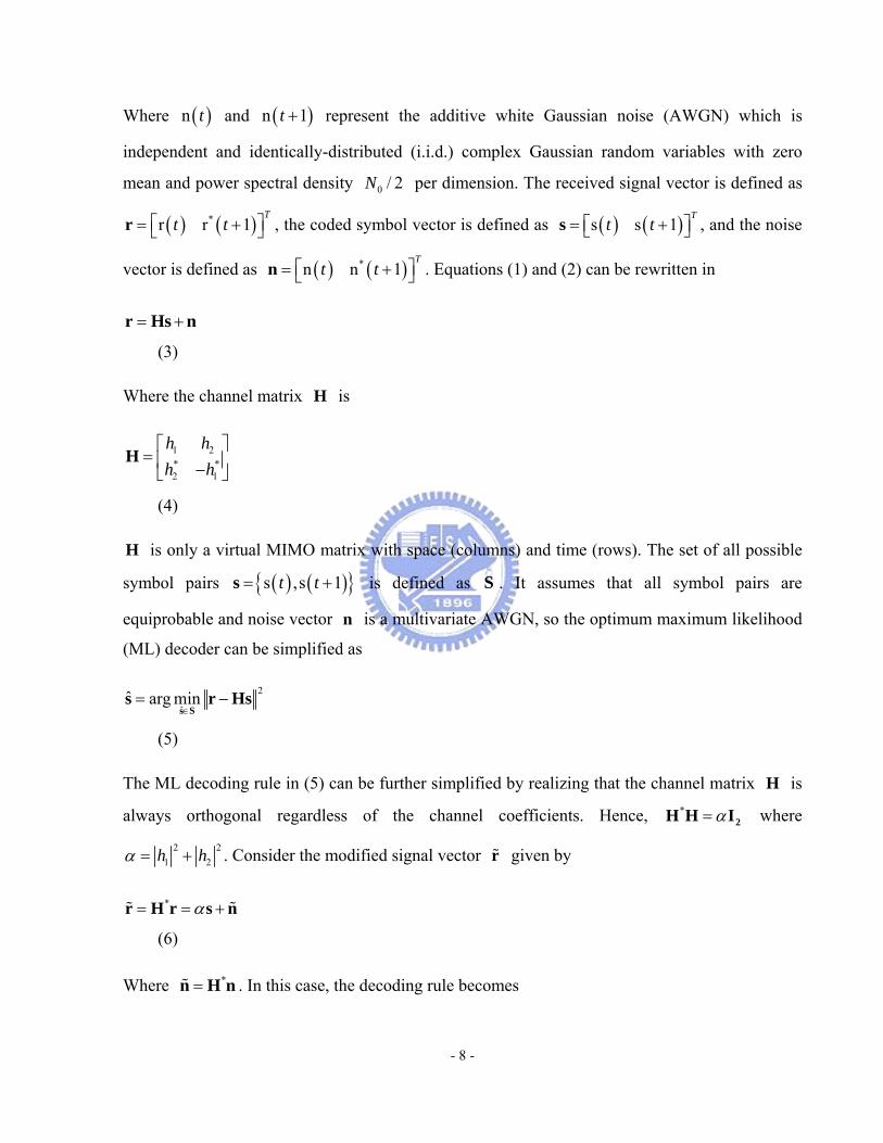

2
ˆˆ arg min ˆα
isin= minus
s Ss r s
(7)
Since is orthogonal it can be easily verified that the noise vector will have a zero mean
and covariance
H n
0 2Nα I Therefore it follows immediately that by using this simple linear
combining the decoding rule in (7) reduces to two separate and much simpler decoding rules for
and ( )s t ( )s 1t +
Initially developed to provide transmit diversity in the MISO case STCs are easily extended to
the MIMO case When the receiver has two antennas such as figure 2-3 the received signal
vector at receive antenna m is mr
12m= sdot + =m m mr H s n
(8)
1 2 2 1
1 2m mm
m m
h hm
h h⎡ ⎤
= ⎢ ⎥minus⎣ ⎦H =
(9)
Where is the noise vector at the two time instants and is the channel matrix from the
two transmit antennas to the mth receive antenna The optimum ML decoder can be represented
by
mn mH
22
ˆ1
ˆ arg min m mmisin=
= minussums Ss r ˆH s (10)
The decision rule in (7) and (10) is applied a hard decision on = sdotr H r and
respectively Therefore as shown in figure 2-3 the received vector after linear combining
can be made soft decision for
2
1m=
= summ mr H mr
ˆmr
( )s t and ( )s 1t + If the STBC is concatenated with an outer
conventional channel code such as convolutional code the soft decisions can be fed to the outer
channel decoder to yield a better performance The extension of the above STBC to more than
two transmit antennas was studied in [17] [19] [20] and [21] A technique was developed for
- 9 -
constructing STBCs that provide the maximum diversity promised by the number of transmit and
receive antennas These codes keep the simple ML decoding algorithm in use based on only
linear processing at the receiver [18] However for general constellation mapper like M-QAM or
M-PSK there is not a STBC with transmission rate one and simple linear processing that will give
the maximum diversity gain with more than two transmit antennas Moreover it was also shown
that such a code where the number of transmit antennas equal the number of both the number of
information symbols transmitted and the number of the slot is needed to transmit the code block
does not exist However for rates less than one such codes can be found and it is also possible to
sacrifice orthogonality in an effort to maintain full rate or one code with more than two transmit
antennas In [22] quasi-orthogonal STBC could preserve the full diversity and full rate at the cost
of a small loss BER and some extra decoding complexity relative to truly orthogonal schemes
232 Spatial Multiplexing Spatial multiplexing can maximize the average data rate over the MIMO system due to each
stream of independent data are transmitted over different antennas Assuming a block of
independent data with size s M Ltimes is transmitted over the M Ntimes MIMO system and the
receiver will obtain where size of is = +r hs n r N Ltimes where L is the length of a block
M is the number of transmit antennas and is the number of receive antennas The optimum
decoding method is ML decoder where the receiver compares all possible combination s of
symbols which could have been transmitted with what is observed
N
ˆˆ arg min=
ss r ˆminushs (11)
The complexity of ML decoder is very high when many antennas or high-order modulations are
adopted Enhanced variants of this like sphere decoding [23] have been proposed Another
popular decoding strategy BLAST (Bell Laboratories Layered Space-Time) or D-BLAST
(Diagonal-BLAST) proposed by [3] D-BLAST employs a diagonally layered coding structure in
which code blocks are dispersed across diagonals in space-time However the diagonal approach
suffers from certain implementation complexity which makes it inappropriate for initial
implementation Some space-time is wasted at the start and the end of a burst that would be
significant when the burst length is short and the complication of the careful avoidance of
catastrophic error propagation is a concern
- 10 -
In [24] vertical BLAST (V-BLAST) was addressed to be implemented in practice Space is the
M points discrete space defined by the M transmit antennas V stands for vertical referring to
layering space-time with consecutive transmitted vector signals a sequence of successive vertical
columns in space-time
Figure 2-4 Spatial Multiplexing Transmitter
A high ndashlevel block diagram of V-BLAST system is shown in figure 2-4 A single data stream is
demultiplex into M substreams and fed to its respective transmitter Each transmitter is an
ordinary QAM transmitter The collection of transmitters comprises in effect a vector-valued
transmitter where components of each transmitted M-vector are symbols drawn from a QAM
constellation Here the same constellation is employed for each substream and that
transmissions are organized into burst of L symbols The power launched by each transmit
antenna is proportional to 1 M so that the total radiated power is constant Inter-substream
coding is not required though conventional coding of the individual substreams is certainly
applied
ChannelEstimator
OptimalOrdering
Nulling ML Detection
Nulling
SymbolCancellation
SymbolCancellation
ML Detection
Figure 2-5 Spatial Multiplexing Receiver
- 11 -
Letting [ ]1 2T
Ma a a=a denote the vector of transmit symbols then the corresponding
received vector is
= +1r Ha n
Where n is a noise vector with components drawn from iid wide-sense stationary processes
with variance 2σ Each substream in turn is considered to be the desired signal and the
remainder is considered as interferers Nulling is performed by linearly weighting the received
signals so as to satisfy some performance-related criterion such as minimum-mean-squared error
(MMSE) or zero-forcing (ZF) The linear nulling approach is viable but nonlinear techniques can
achieve better performance Using symbol cancellation interference from already-detected
components of is subtracted out from the received signal vector As the result effectively
fewer interferers are present in a modified received vector This is somewhat analogous to
decision feed back equalization When symbol cancellation is used the order in which the
components of are detected becomes important to overall performance of the system but it
doesnrsquot have influence when pure nulling is used Under the assumption that components of
are employ the same modulation constellation the component with the smallest receive SNR will
dominate the error performance of the system Choosing the best receive SNR at each stage in the
detection in the detection process leads to the optimum ordering The full V-BLAST detection
algorithm can be described compactly as a recursive procedure shown in Figure 2-5
a
a
a
24 Introduction of MIMO in WiMAX In WiMAX multiple antennas technique is optional but MIMO will become main stream due to
high throughput and low BER In this section how WiMAX supports MIMO with STC will be
introduced
241 STBC in WiMAX In WiMAX two three and four antennas can be employed and matrix A matrix B and matrix C
are defined to support STBC as shown in Table 2-1 In two transmit antennas system matrix A is
applied for transmit diversity and matrix B is applied for spatial multiplexing In three and four
- 12 -
transmit antennas systems matrix A and matrix B is applied for transmit diversity and matrix C
is applied for spatial multiplexing
Table 2-1 STBC Types in WiMAX
2X2 3X3 4X4
Matrix A 1
1
i i
i i
S SS S
+
+
⎡ ⎤minus⎢ ⎥⎣ ⎦
1 2
2 1 3 4
4 3
0 0
0 0
S SS S S S
S S
⎡ ⎤minus⎢ ⎥
minus⎢ ⎥⎢ ⎥⎣ ⎦
1 2
2 1
3 4
4 3
0 00 0
0 00 0
S SS S
S SS S
⎡ ⎤minus⎢ ⎥⎢ ⎥⎢ ⎥minus⎢ ⎥⎢ ⎥⎣ ⎦
Matrix B X
1 2 5 6
2 1 6 5
7 8 3 4
3 0 04
30 04
30 04
S S S SS S S SS S S S
⎡ ⎤⎢ ⎥⎢ ⎥ ⎡ ⎤minus minus⎢ ⎥ ⎢ ⎥⎢ ⎥ ⎢ ⎥⎢ ⎥ ⎢ ⎥minus minus⎣ ⎦⎢ ⎥⎢ ⎥⎢ ⎥⎣ ⎦
1 2 5 7
2 1 6 8
3 4 7 5
4 3 8 6
S S S SS S S SS S S SS S S S
⎡ ⎤minus minus⎢ ⎥minus⎢ ⎥⎢ ⎥minus⎢ ⎥⎢ ⎥⎣ ⎦
Matrix C
1
i
i
SS +
⎡ ⎤⎢ ⎥⎣ ⎦
1
2
3
SSS
⎡ ⎤⎢ ⎥⎢ ⎥⎢ ⎥⎣ ⎦
1
2
3
4
SSSS
⎡ ⎤⎢ ⎥⎢ ⎥⎢ ⎥⎢ ⎥⎣ ⎦
Where the complex symbols to be transmitted be 1x 2x 3x 4x which take values from a
square QAM constellation Let for ji i iI iQS x e S jSθ= = + 1 28i = where 1 1tan
3θ minus ⎛ ⎞= ⎜ ⎟
⎝ ⎠ and
This space-time-frequency code can be
decoded by ML method
1 1 3I QS S jS= + 2 2 4I QS S jS= + 3 3 1I QS S jS= + 4 4 2I QS S jS= + 5 5 7I QS S jS= +
6 6 8I QS S jS= + 7 7 5I QS S jS= + 8 8 6IS S S= + Q
- 13 -
Antennas selection and antennas grouping can used for spatial multiplexing and transmit
diversity respectively In matrix B and matrix C the MIMO system can select coding method
between vertical coding and horizontal coding Vertical coding indicates transmitting a single
FEC encoded stream over multiple antennas so the number of encoded stream is always 1 such
as Figure 2-6 and Figure 2-8 Transmitting multiple separately FEC encoded stream over multiple
antennas is horizontal encoding and the number of encoded stream is more than 1 such as Fig
2-7 and Fig 2-9 A stream is defined as each information path encoded by STC encoder that is
passed to subcarrier mapping and send through one antenna A layer is defined as an
information path fed in STC encoder as an input hence the number of layers in a system with
vertical encoding is one but in case of horizontal coding it depends on the number of encoding
and modulation path It means that only horizontal encoding can support multi-user transmission
Table 2-2 defines the mode of downlink operation which describes all transmission methods in
IEEE 80216e
Table 2-2 Downlink MIMO Operation Mode
Number of
transmit
antennas
Matrix
indicator
Num of
layers
Number of
users
Encoding
type Rate
2 A 1 1 STTD 1
2 B 1 1 Vertical
encoding 2
2 B 2 1 Horizontal
encoding 2
2 B 2 2 Horizontal
encoding 2
4 A 1 1 STTD 1
- 14 -
4 B 1 1 Vertical
encoding 2
4 B 2 1 Horizontal
encoding 2
4 B 2 2 Horizontal
encoding 2
4 C 1 1 Vertical
encoding 4
4 C 4 1 Horizontal
encoding 2
4 C 4 gt1 Horizontal
encoding 4
Table 2-3 defines the mode of uplink operation which describes all transmission methods in IEEE
80216e During up transmission a MS uses most two antennas
Table 2-3 Uplink MIMO Operation Mode
Number of
transmit
antennas
Matrix
indicator
Num of
layers
Number of
users
Encoding
type
Rate
1 B 2 2 Collaborative 1 per users
2 B 1 1 Vertical
encoding
2
2 A 1 1 STTD 1
- 15 -
Figure 2-6 Transmitter of Matrix A for 2 3 or 4 Transmit Antennas and Matrix B for 3 or 4 Transmit Antennas
Figure 2-7 Transmitter of Matrix B with Horizontal Encoding for 3 or 4 Transmit Antennas
Figure 2-8 Transmitter of Matrix C with Vertical Encoding for 2 3 or 4 Transmit Antennas
Figure 2-9 Transmitter of Matrix C with Horizontal Encoding for 2 3 or 4 Transmit Antennas
- 16 -
242 MIMO Coefficient The STC scheme for two antennas may be enhanced by using four antennas at the transmission
site like combination of STC and AAS as shown in Fig 2-10 Two first antennas Antenna 0 and
Antenna 1 transmit the signal as defined in transmit diversity or in spatial multiplexing and the
two second antennas Antenna 0rsquo and Antenna 1rsquo transmit two first antennas signal with a
complex multiplication factor The BS may change the antennas weights using feedback from the
user The transmitter can get the MIMO coefficient which be represented by Fig 2-11 from
feedback
00
jA e φ
11
jA e φ
Figure 2-10 The STC Scheme for Two Antennas Enhanced by Using Four Antennas
- 17 -
Figure 2-11 Mapping of MIMO Coefficients for Quantized Precoding Weights for Enhanced Fast MIMO Feedback Payload Bits
This method does not change the channel estimation process of the user Therefore this scheme
could be implemented without any changes made to the STC users
243 MIMO Feedback in WiMAX In WiMAX system all transmission setup is decided by the BS A BS needs information and
control signals to maintain transmission A MS can send feedbacks either as a response to
feedback requests of a BS or as an unsolicited feedback Feedbacks and feedback requests can be
sent through the MAC layer and the PHY layer The MIMO system need more information and
control signals because of more complex transceiver of MIMO system
- 18 -
MIMO Feedback requests are sent by a BS to ask MS reporting the information about MIMO
parameters In the MAC layer they can be brought in feedback request extended subheader and
fast feedback allocation subheader In the PHY layer the feedback-polling information element
(IE) CQICH allocation IE and CQICH allocation enhanced IE in the uplink map can trigger off
feedback of MSs
In the MIMO system there are three important parameters MIMO mode MIMO coefficients
and SNR which need to be fed by users MSs can report information in the MAC layer and
employ fast feedback channel or fast feedback enhanced channel to feed parameters in the PHY
layer Feedback in MAC layer is allocated by feedback polling IE and feedback request extended
subheader and in PHY layer is allociated in fast feedback channel and enhanced fast feedback
channel which include fast MIMO feedback (MIMO coefficient) mode selection feedback and
effective CINR feedback indicated in fast feedback allocation subheader CQICH allocation IE
CQICH allocation enhanced IE
244 MIMO Control in WiMAX In the MIMO transmission a BS control MIMO setup including number of antennas midamble
presence matrix indicator number of layers and pilot pattern indicator A BS sets MIMO
transmission through STC downlink zone IE MIMO downlink basic IE MIMO downlink
enhanced IE MIMO uplink basic IE and MIMO uplink enhanced IE The MIMO control
information elements is shown in Table 2-4
- 19 -
Table 2-4 MIMO Control Information Elements
function
STC downlink zone IE Number of antennas
Midamble presence
Matrix indicator
MIMO downlink basic IE Matrix indicator
Number of layers
MIMO downlink enhanced IE Matrix indicator
Number of layers
MIMO uplink basic IE Matrix indicator
Collaborative indicator
MIMO uplink enhanced IE Matrix indicator
pilot pattern indicator
- 20 -
Chapter 3 Simulation Setup
In this chapter the IEEE 80216e system level simulation platform with MIMO technologies will
be described The details of system architecture and simulation parameters are going to be
presented Then the link budget such as path loss and shadow fading in the platform is suitable
for IEEE 80216e standard The setting of basic radio resource managements will be described in
this chapter Finally the traffic models of simulation are introduced The setting and the structure
of the simulation platform is referred from [25]
31 Simulation architecture In the simulation of a mobile system the interference from other cells is an important element
that would affect the overall performance Hence the effect needs to be considered into the
simulation When the number of simulation cells increase it causes high load of computation and
needs long simulation time Considering the tradeoff between accurate simulation and computing
cost two-tier interference is appropriate According to approximate the cell coverage with a
hexagon we consider nineteen cells in our simulation as shown in Figure 3-1 in which only the
central cell completely has two-tier interference cells and the other cells can not find out the
symmetric two-tier interference cells Even if nineteen cells are simulated only one statistic
simulation value of the central cell can be referred that is lower simulated efficiency Therefore
a wrap around technique as shown in Figure 3-2 is adopted to make any of nineteen cells owns
complete two-tier interference cells The main ideal is the lacks of any two-tier interference cells
of a specific cell are copies from the simulated cells which are besides the two-tier interference
cells of the specific cell Through the clever arrangement every cell has complete and symmetric
two-tier interference cells Because the cell owns whole interference after wrap around the
statistic simulation value of nineteen cells would be meaningful
- 21 -
Figure 3-1 Cell Structure of System
Figure 3-2 Wrap Around
The cell radius is 1 km and the total cell bandwidth is 10 MHz This approximate cell coverage is
a result from a plan of Link Budget In the simulation platform a cell is divided into three sectors
as shown in Figure 3-3 Each sector has the different antenna direction and a regular pattern of
deployment The sector architecture in 80216e system can reduce the transmission power of BS
antenna and intercell interference Furthermore there is a small part of intercell interference in
different sectors of distinct BSs due to subcarrier permutation This characteristic is very difficult
to simulate so instead of it a sector would only produce interference to other sectors which have
- 22 -
the same direction due to sectors of the same direction have the same subchannel The cellrsquos
frequency reuse factor in our simulation platform will be set to 1 as shown in Figure 3-3 and
needs 10 MHz bandwidth
Figure 3-3 Sector Deployment and Frequency Reuse Factor
In our simulation platform the setting of antenna pattern uses the 3GPPrsquos model [3GPP] as
shown in Figure 3-4
( )2
3
min 12 mdB
A Aθθθ
⎡ ⎤⎛ ⎞⎢= minus times⎜ ⎟⎢ ⎥⎝ ⎠⎣ ⎦
⎥
B
(12)
Where and 180 180θminus le le 3 70dBθ = 20mA d=
- 23 -
3 Sector Antenna Pattern
-25
-20
-15
-10
-5
0
-120 -100 -80 -60 -40 -20 0 20 40 60 80 100 120
Azimuth in Degrees
Gai
n in
dB
Figure 3-4 Antenna Pattern for 3-sector Cells
32 The Architecture of Frame Transmission In the thesis the downlink transmission is focused and the OFDMA technique with TDD mode is
adopted The IEEE 80216 standard can support an asymmetric downlink and uplink transmission
of TDD mode which adjusts the ratio according to the traffic loading of downlink and uplink
transmission In the simulation the ratio of downlink to uplink transmission is29 to 18 and the
frame length is 5 ms The frame structure is 1024-FFT OFDMA downlink carrier allocations
-PUSC mode defined in the standard and the carrier distribution is shown in Table 3-1 In the
1024 subcarriers only 720 subcarriers carry data information and other subcarriers are used for
guard band pilot and dc subcarrier
- 24 -
Table 3-1 OFDMA Downlink Parameter
Parameter Value
System Channel Bandwidth 10 MHz
Sampling Frequency 112 MHz
FFT Size 1024
Subcarrier Frequency Spacing 1094 kHz
Useful Symbol Time 914 microseconds
Guard Time 114 microseconds
OFDMA Symbol Duration 1029 microseconds
Frame duration 5 milliseconds
Number of OFDMA Symbols 48
DL PUSC Null Subcarriers 184
DL PUSC Pilot Subcarriers 120
DL PUSC Data Subcarriers 720
DL PUSC Subchannels 30
The length and number of OFDMA symbols are defined according to WiMAX Forum [25] and
[26] For 10MHz bandwidth and 1024 FFT sizes the symbol period should be 1029 μs and there
will be 47 OFDMA symbols per frame According to the ratio of downlink to uplink transmission
there are 24 symbols per downlink frame Due to the definition of PUSC in IEEE80216e two
symbols with one subchannel form one slot There are 12 slots in a downlink frame and 10
subchannels per sector (303 = 10) Hence there are 120 slots per downlink frame to transmit
data
- 25 -
33 Link Budget The link budget settings of downlink transmission in our simulation are as far as possible to
match the Mobile WiMAX [25] environment In [25] it makes deployment scenario assumptions
for 80216e such as Table 3-2 In the simulation the outdoor vehicular scenario is adopted
which the BS transmitted power is 43 dBm the BS antenna gain is 15 dBi the MS antenna gain
is -1dBi on the downlink transmission The common usage value of thermal noise density is
-17393 dB Hz The receiver noise figure of MSs is 7 dB [25]
Table 3-2 Link Budget Parameter of Mobile WiMAX
Scenario
Parameter
Indoor Outdoor to indoor Outdoor vehicular
BS Tx power 27 dBm (05 W) 36 dBm (4 W) 43 dBm
MS Tx power 17 dBm 17 dBm 23 dBm
BS ant gain 6 dBi 17 dBi 15 dBi
MS ant gain 0 dBi 0 dBi -1 dBi
BS ant height 15 m 30 m
In wireless channel the transmitted signals will suffer the fading effect which can change the
original signals The fading can be divided into two types large scale and small scale Large
scale fading which contains pathloss and shadow fading would affect SINR and small scale
fading which is composed of multipath effect Doppler effect and spatial correlation frequency
correlation) has not influence of SINR because average of the small scale during a frame time is
zero In the simulation slow fading without spatial correlation and Doppler effect is adopted The
pathloss model is used to present the signal strength decreases with increasing distance between - 26 -
transmitter and receiver In 3GPP spatial correlation channel (SCM) [27] it provides several
pathloss models such as Table 3-3 Suburban macro scenario is adopted in the simulation
Table 3-3 Environment Parameters in SCM
Channel Scenario Suburban Macro Urban Macro Urban Micro Lognormal shadowing standard deviation SFσ 8dB 8dB NLOS 10dB
LOS 4dB Pathloss model (dB) d is in meters 315 + 35log10(d) 345 + 35log10(d) NLOS 3453 + 38log10(d)
LOS 3018 + 26log10(d)
The main reason forms shadow fading is from the shelters like buildings or mountain on the
signal transmitted path According to the test result of the real wireless environment we can
know the variant of shadow fading is a log-normal distribution statistically Hence we can use
the log-normal distribution to produce the shadow fading effect The standard deviation of this
distribution is based on the simulation environment In the simulation the standard deviation is 8
dB due to SCM model [27] When the user is fixed the shadow fading effect will not alter On
the other hand the shadow fading changes in different locations of the mobile user In the
different simulation points we can use the log-normal distribution to produce a value for the
shadow fading However the time between two neighbor simulation points is very small so that
the mobile user location will not change very obvious even at high mobile speed It means the
variance the shadow fading will not be large and have a correlated relationship between two
neighbor time points Hence we use the concept of a correlation model called Gudmundsonrsquos
correlation model [28]
( ) exp( ln 2)cor
xx
dρ = minus (13)
where ρ is the auto-correlation constant between two simulation sample points x is the
distance of two sample points and is a function of sampling times between them sampling
duration and user speed The cord is de-correlation distance and the values in the suburban
macro urban macro and urban micro environments are 200m 50m and 5m respectively In the
- 27 -
simulation we use 50m as our parameter Using log-normal distribution and correlation model
the simulation can get more actual shadow fading
Figure 3-5 SINR Computation Flow
In Figure 3-5 we present the flow of signal-to-interference and noise ratio (SINR) computation
The OFDMA technique uses the multiple carriers to transmit signal and we should compute
carrier-to-interference and noise ratio (CINR) not SINR But the MSs of 80216 system with
PUSC or FUSC mode only compute and report the sum of received CINR per carrier to BS not
individual CINR Hence the SINR and CINR are the same under these conditions Finally the
mobility model we use is like below The MS speed is 30 kmhr Probability to change direction
is 02 when position update and maximum angle for direction update is 45o
34 Performance Curve After CINR calculation modulation and coding scheme need to be decided How to select
modulation and coding scheme is based on BER or PER which is calculated in physical layer as
shown in Figure 3-6 Performance curve can map received to BER or PER and includes small
scale fading In the simulation small scale fading contains multipath effect frequency correlation
and performance curve is produced based on IEEE 80216e standard as shown in Figure 3-7 and
Figure3-8 from Prof Wu
- 28 -
Figure 3-6 Physical Layer Block Diagram
0 5 10 15 20 2510-7
10-6
10-5
10-4
10-3
10-2
10-1
100
CINR (dB)
BE
R
SISO
QPSK16QAM64QAM
Figure 3-7 SISO Performance Curve
- 29 -
0 5 10 15 20 25 30 35 40 45 5010-6
10-5
10-4
10-3
10-2
10-1
100
CINR
BE
R
4X4 MIMO A-QPSKA-16QAMA-64QAMB-QPSKB-16QAMB-64QAMC-QPSK-MLC-16QAM-MLC-64QAM-MLC-QPSK-VBLASTC-16QAM-VBLASTC-64QAM-VBLAST
Figure 3-8 4X4 MIMO Performance Curve
35 Basic Radio Resource Management The purpose of radio resource managements is to raise the efficiency and reliability of wireless
transmission In the performance analysis the basic radio resource management is constructed
and described as following
351 Rate Control The adaptive modulation and coding scheme is a major method to keep the quality of wireless
transmission Due to trade off between efficiency and robustness IEEE80216e system can
dynamically adjust modulation coding scheme depends on the carrier to interference plus noise
ratio (CINR) condition of the radio link It supports multiple modulation methods Quadrature
Phase Shift Keying (QPSK) 16-state Quadrature Amplitude modulation (16-QAM) and 16-state
Quadrature Amplitude modulation (64-QAM) and several coding schemes like Convolution
- 30 -
Code (CC) Low Density Parity Check Code (LDPC) Block Turbo Code (BTC) and
Convolution Turbo Code (CTC) In the simulation the coding scheme is used to correct errors in
the receiver and only convolution code (CC) with 12 code rate is applied From 42 one slot
carries 48 96 and 144 bits by using QPSK 16-QAM and 64-QAM respectively
Figure 3-9 Example of Mapping OFDMA Slots toSsubchannels and Symbols in The Downlink PUSC Mode
Data Region is a two-dimensional allocation which contents a group of contiguous subchannels
and OFDMA symbols All the allocation refers to logical subchannels The minimum unit of data
mapping is an OFDMA slot Based on standard how many and which slots should be assigned to
a transmission is decided by BS and there are different mechanisms in downlink and uplink
transmission In downlink resource allocation the system according to the data size tries to fulfill
the slots first in frequency domain After the frequency domain is fulfilled then it changes to the
- 31 -
next time domain to continuously fulfill slots In other words the data mapping method is
frequency first as shown in Figure 3-9
Figure 4-7 Example o mapping OFDMA slots to subchannels and symbols in the downlink PUSC
mode
352 Subcarrier Permutation Subcarrier permutation is a method to assign frequency subcarriers into subchannels The
allocation of subcarriers to subchannels is accomplished via permutation rule
Partial Usage of Subchannels (PUSC) which is the distributed subcarrier permutation is
applied in the simulation Distributed permutation means the subcarriers belonged to a
subchannel are selected pseudo randomly from all subcarriers It can average intercell
interference and avoid fading effect PUSC can be used both in downlink and uplink It will
group subcarriers first then choose subcarriers per group and each group only provides one
subcarriers to form a subchannel It also use distributed permutation mode Hence the
interference of one slot produced by the other cells will be dispersed to all subframe
353 Scheduling Methods Based on the information mentioned before BS will do the scheduling decision and form
DL-MAP and UL-MAP to indicate the scheduling result System could consider the QoS
requirement of different service and their channel condition to do the scheduling decision and a
good scheduling algorithm shall utilize the resource well and meet the different usersrsquo
requirement In the IEEE80216e standard it doesnrsquot define the scheduling information and this
part is left for design And a proposed scheduling algorithm will be discussed in detail in this
thesis
Some scheduling algorithms proposed by [29] [30] [31] [32] and [33] are applied in the
simulation Different scheduling algorithms have different targets to achieve Some of them want
to achieve fairness and some of them hope to maximize throughput or maintain the QoS These
algorithms have their own advantages However they have disadvantages in some aspects too
3531 Round-Robin (RR)
- 32 -
In the round-robin scheduling algorithm a system schedules packets by users in a fixed sequence
irrespective of the channel condition and services requirement This algorithm provides fairness
but ignore the channel condition and QoS requirement It is hard to be used in mix-traffic system
due to different QoS requirement
3532 MaxCINR
MaxCINR scheduling algorithm schedules packets which belonged to the user with better CINR
much better channel condition The kind of scheduling algorithm takes channel condition into
consideration and may provide good multiuser diversity to enhance system throughput and
decrease transmission time due to efficient transmission However it is less fairness If the power
control doesnrsquot implement well some users might never get opportunity to transmit data Besides
it canrsquot provide QoS guarantee especially to real-time service which QoS definition is usually
delay bound consideration System will select user m that fulfill
( )m arg max CINRmmt = ( )t (14)
3533 Proportional Fair (PF)
This algorithm considers channel condition and fairness across users It provides a tradeoff
between system throughput and user fairness The scheduling decision will follow a ratio which
is instantaneous data-rate over average data-rate and pick larger user m
( ) ( )( )
Rm arg max
Sm
mm
tt
t= (15)
( ) ( ) ( ) ( )1 1S 1 S 1 Rm m mt t tW W
δ⎛ ⎞= minus minus + minus⎜ ⎟⎝ ⎠
t m (16)
where ( )Rm t denotes the achievable instantaneous data rate for user m ( )Sm t denotes the
moving average of data-rate at user m and W donates the length of moving average This
algorithm provides both fairness and channel condition concerns but it lacks QoS guarantee
especially for real-time service
- 33 -
3534 Early Deadline First (EDF)
This algorithm considers completely the delay constraint It ignores the channel quality so it
might not use bandwidth efficiently However it can provide strict QoS guarantee for
delay-sensitive service because it will transmit packet first which is much closer to their delay
bound System will transmit packet belonged to user if m
( arg min mmm DB Age= minus )Tminus (17)
where DB means delay bound Age is the time that the packet stayed in MAC and is the
transmission time for users in the current frame
mT
In non-real-time service there is no delay bound requirement but they have the minimum
reserved rate requirement Although non-real-time service can tolerate delay it still must be
transmitted in an acceptable rate A new QoS criterion is called ldquosoft delay boundrdquo defined by
[34] Soft delay bound is not only still related to the definition of minimum reserved rate but it
translates the minimum reserved rate concept into time concept With the common definition for
both real-time and non-real-time services it will be much easier to do the scheduler design
The minimum reserved rate means how many data should be transmitted in a certain period to
meet the QoS requirement In another aspect of the definition how many time before should
system transmit the known size packet will meet the QoS requirement And that time will be the
soft delay bound for non-real-time service
__ _min _ _ _
packet sizesoft delay boundimum reserved traffic rate
= (18)
The soft delay bound will be an indication of the minimum performance that the non-real-time
service should achieve If the packet be transmitted successfully before the soft delay bound it
means the packet meets the QoS requirement However it doesnrsquot mean that the non-real-time
service can only achieve the defined performance If there are still resource could be used the
non-real-time service can have better performance Maybe the packet can be transmitted much
earlier before the soft delay bound
- 34 -
It is called ldquosoft delay boundrdquo because the different characteristic between real-time and
non-real-time service If the real-time service exceeds the delay bound the packet will be
dropped because it is useless even However non-real-time service must focus on the correctness
It can tolerate delay but doesnrsquot like data loss Therefore system will still transmit the
non-real-time service packet even if it exceeds the soft delay bound
Besides the drop and transmit issue the soft delay bound of non-real-time service will be
accumulated across the packets belonged to the same user It can be expressed in the following
formula P denotes the packet size
( )1 2 nP P Pminimum_reserved_rate
t+ + +
ge (19)
( )1 2_ _ nP P Psoft delay bound
minimum_reserved_rate+ + +
le (20)
It means a single user might have several packets to be transmitted The soft delay bound will
accumulate across packets If the first packet is transmitted much earlier before itsrsquo soft delay
bound The second packet of the user will have much longer soft delay bound because it take
benefit from the first packetrsquos fast transmission However if the first packet is transmitted really
late even after the required soft delay bound it means the packet doesnrsquot meet the QoS
requirement Besides this it will influence the next packet because the next packet will have
shorter delay bound than normal because the former packet takes much longer time
354 Segmentation and Packing The MAC PDU is a data exchanged unit between the MAC layer of the BS and MSs A MAC
PDU consists of a 48bit MAC header a variable length data payload and an optional 32 bits
Cyclic Redundancy Check (CRC) Sometimes some MAC PDU will not include payload and
CRC bits These kinds of PDUs are used only in the uplink to transmit control message Those
MAC signaling headers include bandwidth request uplink transmit power report CINR report
CQICH allocation request PHY channel report uplink sleep control SN report and feedback
functionalities MAC PDUs also include some subheaders Those subheaders will be inserted in
- 35 -
MAC PDUs following the generic MAC header Those subheaders help system perform grant
management packing ARQ feedback etchellip
In IEEE 80216e system MAC SDUs coming from CS will be formatted according to the MAC
PDU format in the CPS possibly with fragmentation and packing Thatrsquos due to the precious
radio resources and system hopes to utilize the resources efficiently
Fragmentation process means to divide a SDU into different PDUs payload areas That is because
the MAC PDU size is limited by standard 2048 bytes Besides larger PDU size may causes error
occurs more easily Therefore divide SDU properly according to the channel condition will avoid
transmission errors and save the resource used for retransmission Figure 3-10 shows the process
of fragmentation
Figure 3-10 Segmentation
Packing process is to pack several SDUs into a single PDU payload In this way system
may avoid resource waste due to the overhead caused by MAC header and CRC Figure 3-11
shows the process of packing
Both processes may be initiated by either a BS for a downlink connection or a MS for and uplink
connection
- 36 -
Figure 3-11 Packing
In the simulation a MAC SDU is generated according to traffic model Then system will
segment a SDU into PDUs or pack SDUs into a PDU to satisfy a fixed PDU size 180 Bytes
which is decided by slot size and performance curve Then PER can be calculated by
(1 1 bitsPER BER= minus minus ) (21)
BER is available by channel condition feedback and performance curve mapping The rate
control is used to satisfy the target PER which is could different in each application
In the simulation packing is not applied because there are not so small packets which need to be
packed The segmentation method wants to use last slots to transmit a packet First it calculates
how many slots should be occupied when a packet is not segmented and size of padding in a
burst Then it exploits the padding of a burst to decided number of PDU and PDU size For
example in Figure 3-12 a packet can be segmented into two PDUs occupies the same slots as a
packet without segmentation but have smaller size of each PDU However it needs three slots to
transmit when a packet is segmented into three PDUs so that throughput or throughput could
decrease
- 37 -
Figure 3-12 Segmentation Comparison
355 Others 3551 Power Control
The BS launches signals with maximum and fixed power The power of each subcarrier is equal
3552 Handoff method
In the thesis hard handoff which is ldquoBreak-Before-Makerdquo is applied since handoff is not a
weight-bearing point in the simulation
3553 ARQ retransmission
In the simulation we only implement the ARQ retransmission and donrsquot use the HARQ When
the PDU comes about error the ARQ retransmission will work However if system finds out that
the retransmission exceeds packetrsquos delay bound of the service it will drop the packet because it
is meaningless to retransmit the PDU The number of retransmission times is decided based on
- 38 -
the type of applications For streaming service and non-real-time service the retransmission
times are three and for voice service the retransmission time is one Thatrsquos because the delay is
core factor in QoS for voice service and the error rate is the core factor in QoS for streaming and
non-real-time servicel
36 Traffic Model In IEEE 80216e standard the downlink data traffics are divided into four QoS classes such as
real-time CBR real-time VBR delay-tolerant VBR and BE The details are described in [25] In
the simulation we build FTP service to stand for delay-tolerant VBR service voice and
streaming service for real-time VBR The FTP traffic model adopts 3GPP2 model [35] as shown
in Table 3-4 Both of the non-real-time servicesrsquo minimum reserved rate will be set to 60kbps
according to [36] The VoIP traffic model uses G729 codec [37] as shown in Table 3-5 The FTP
services use TCPIP protocol to transmit so the FTP packet needs to add 20 bytes TCP header
and 20 bytes IP header The VoIP services user RTPUDPIP protocol to transmit The VoIP
packet must add 12 bytes RTP header 8 bytes UDP header and 20 bytes IP header
Table 3-4 FTP Traffic Model
File Size Truncated
Lognormal
Mean = 2 Mbytes
Std Dev = 0722 Mbytes
Maximum = 5 Mbytes
Reading Time exponential Mean = 180 sec
Table 3-5 VOIP Traffic Model
codec Framesize(byte) Interval(ms) Rate(bps) Delay bound(ms)
G729-1 200 200 8k 200
- 39 -
Mobile WiMAX supports VOIP and FTP service with varied QoS requirements as described in
Table 3-6
Table 3-6 Applications and Quality of Service
Table 3-6 QoS Class Applications QoS Specifications
UnSolicited Grant Service
(UGS)
VoIP Maximum sustained rate
Maximum latency
tolerance
Jitter tolerance
Non-Real-Time Polling
Service
FTP Minimum Reserved Rate
Maximum Sustained Rate
Traffic Priority
37 Simulation Parameters Finally we use Table X to summarize this chapter and present the arrangement of the parameter
setting in our simulation platform
Table 3-7 The Parameter Setting in Simulation Platform
Parameters Value
Number of 3-Sector Cells 19
Operating Frequency 25 GHz
Duplex TDD
- 40 -
Subcarrier Permutation PUSC
Channel Bandwidth 10 MHz
BS-to-BS Distance 2 kilometers
Minimum Mobile-to-BS Distance 36 meters
Antenna Pattern 70deg (-3 dB) with 20 dB front-to-back ratio
BS Height 32 meters
MS Height 15 meters
BS Antenna Gain 15 dBi
MS Antenna Gain -1 dBi
BS Maximum PowerAmplifier Power 43 dBm
MS Maximum Power Amplifier Power 23 dBm
Number of BS TxRx Antenna Tx 4 Rx 4
Number of MS TxRx Antenna Tx 4 Rx 4
BS Noise Figure 7 dB
MS Noise Figure 4 dB
Modulation Scheme QPSK 16QAM 64QAM
Channel Coding Convolutional Code
Interference Model average interference model for PUSC
Link adaptation CQI Feedback Error free
Path Loss Model Loss (dB) =350log(R)+315
(R in m)
- 41 -
Lognormal Shadowing Standard Deviation 8 dB
Correlation distance for shadowing 50m
MS Mobility 30 kmhr
Spatial Channel Model Slow fading with Uncorrelated Cell Configuration 3 SectorsCell
Frequency Reuse 1X3X3
Traffic Type Full Buffer
Scheduler RR MaxCINR PR EDF
Antenna Configuration 1X1 4X4
DL MIMO Support TD SM
MIMO Switch Adaptive MIMO switch
Coding CC
Frame Overhead 9 OFDMA symbols (5DL 3UL 1TTG)
Data Symbols per Frame 39
DLUL Partition 2415
- 42 -
Chapter 4 Simulation Result
In this chapter we show the system level simulation results of MIMO systems in different
downlink scheduling algorithms The scheduling algorithms include Early Dead First
Proportional Fair Maximum CINR and Round Robin We investigate the throughput
performance and some QoS-associated factors such as minimum reserved rate for non-real-time
services and packet loss rate for real-time services
41 Spatial Multiplexing in Different Scheduling Methods In the simulation there are two types of receivers ML and VBLAST which car support Spatial
Multiplexing In this section the spatial multiplexing utilization in different scheduling will be
discussed The utilization is defined as
411 VOIP Traffic Service
VOIP
000
050
100
150
200
250
300
350
20 40 60 80 100 120 140 160 180
users per 3-sector cell
VB
LA
ST
Uti
liza
tion
EDFRRMAXCINRPF
Figure 4-1 VBLAST Utilization for Real Time Service
- 43 -
In VOIP traffic service Figure 4-1 shows spatial multiplexing utilization with VBLAST in
different scheduling is almost the same The spatial multiplexing utilization is defined as
following
_ __ _SM
SM transmission timesUtotal transmission times
= (22)
There is the same result when a ML receiver is employed as shown in Figure 4-2 because a
frame can not be filled to the full when average packet-loss rate achieves upper bound When
approximately 180 users per cell make average packet-loss rate arrive upper bound channel
utilization of each scheduling method is around 77 as shown in Figure 4-3 The channel
utilization is defined as following
__ch
occupied slotsUtotal slots
= (23)
The packet size of VOIP traffic service is small so the channel utilization is dominated by
number of users in a BS In the simulation users are randomly deployed hence each BS doesnrsquot
have the same users When the channel is full in some BSs the packet-loss rate is the proportion
of full channel BSs
In the simulation Spatial multiplexing Utilization with ML receivers is much higher than spatial
multiplexing utilization with VBLAST receivers It means that the ML receiver is more complex
but more efficient
- 44 -
VOIP
000
1000
2000
3000
4000
5000
6000
7000
8000
20 40 60 80 100 120 140 160 180 200
users per 3-sector cell
ML
(C)
Uti
liza
tion
EDFRRMAXCINRPF
Figure 4-2 Utilization of Spatial Multiplexing with ML Receiver for Real Time Service
750
760
770
780
790
800
180
users per 3-sector cell
Channel Utilization EDF_VBLAST
EDF_ML
RR_VBLAST
RR_ML
MAXCINR_VBLAST
MAXCINR_ML
PF_VBLAST
PF_ML
Figure 4-3 Channel Utilization for Real Time Service
- 45 -
412 FTP Traffic Service The packet size is large in the FTP traffic service hence about 20 user per cell can almost fill
every frame with data as shown in Figure 4-4 The spatial multiplexing utilization obviously
relates to the characteristic of each scheduling method as shown in Figure 4-5 and Figure4-6
Spatial multiplexing utilization of EDF method decrease when users per BS increases since users
with bad RF condition have higher transmission priority The MAXCINR method has the highest
spatial multiplexing utilization because spatial multiplexing is employed by high CINR users
The PF method considers both CINR and average data rate hence the spatial multiplexing
utilization lightly decreases when number of users increases Every user has the same
transmission priority when the BS adopts RR scheduling method Therefore all users transmit
data in sequence and spatial multiplexing utilization is almost at any user per cell Spatial
multiplexing utilization of FTP traffic service is higher spatial multiplexing utilization of VOIP
traffic service in every scheduling method A VOIP packet arrives during fixed time hence the
user with high CINR spends more time than the user the low CINR to wait the next packet after
the packet has transmitted The user with high CINR may not successively transmit data in every
frame However the user with FTP traffic service can continuously transmit data in every frame
because the next packet arrives after the packet has transmitted
- 46 -
965
970
975
980
985
990
20
users per 3-sector cell
Channel Utilization EDF_VBLAST
EDF_ML
RR_VBLAST
RR_ML
MAXCINR_VBLAST
MAXCINR_ML
PF_VBLAST
PF_ML
Figure 4-4 Channel Utilization for Non-real Time Service
FTP
00
50
100
150
200
250
300
350
400
450
20 40 60 80 100 120
users per 3-sector cell
VB
LA
ST
Uti
liza
tion
EDFRRMAXCINRPF
- 47 -
Figure 4-5 VBLAST Utilization for FTP Traffic Service
FTP
00
200
400
600
800
1000
1200
20 40 60 80 100 120
users per 3-sector cell
ML
(C)
Uti
liza
tion
EDFRRMAXCINRPF
Figure 4-6 Utilization of Spatial Multiplexing with ML Receiver for FTP Traffic Service
42 QoS of Different Receivers In the thesis the downlink performance of Mobile WiMAX with MIMO technique which
includes three different receivers is investigated in terms of VoIP and FTP and we also compare
their QoS in different scheduling methods The indication of QoS is defined as minimum
reserved rate for non-real-time service (FTP) and packet loss rate for real-time service (VoIP)
Minimum reserved rate is the percentage of users who donrsquot meet the QoS requirements Packet
loss rate indicates the percentage of packets exceeding its delay bound
421 VOIP Traffic Service Figure4 -7 Figure4-8 Figure 4-9 and Figure 4-10 show the results in EDF RR MAXCINR and
PF scheduling methods respectively The results in EDF and RR scheduling methods are that
throughput can be improved about 42 by using MIMO technique The throughput can increase
- 48 -
46 by employing MIMO technique in MAXCINR and PF scheduling methods The
performance of MAXCINR and PF scheduling methods can be improved lightly more than in
EDF and RR scheduling methods because the transmission rate is considered in MAXCINR and
PF scheduling methods
VOIP with EDF
000
050
100
150
200
250
300
350
400
450
20 40 60 80 100 120 140 160 180 200
users per 3-sector cell
Los
s R
ate
SISOVBLASTMLAB
Figure 4-7 Packet Loss Rate with EDF for Real Time Service
In each scheduling method different receivers in MIMO transmission almost have the same
capacity The MIMO transmission which only employs transmit diversity has lightly better
throughput than which employs transmit diversity and spatial multiplexing with VBLAST in high
packet loss rate since users using VBLAST have higher PER than using transmit diversity in
high CINR condition Using spatial multiplexing can not significantly increase throughput even if
the ML receiver is employed It is because the channel utilization is not full when packet loss rate
achieves upper bound as specified in 411 and low CINR users dominate the throughput A
packet of QPSK and matrix A needs to occupy 13 slots but a packet of 64QAM and matrix B
occupies 3 slots Spatial multiplexing can only increase transmission in high CINR condition but
can not improve in low CIRN condition
- 49 -
VOIP with RR
000
050
100
150
200
250
300
350
400
20 40 60 80 100 120 140 160 180
users per 3-sector cell
Los
s R
ate
SISOVBLASTMLAB
Figure 4-8 Packet Loss Rate with RR for Real Time Service
VOIP with MAXCINR
000
100
200
300
400
500
600
20 40 60 80 100 120 140 160 180 200
users per 3-sector cell
Los
s R
ate
SISOVBLASTMLAB
- 50 -
Figure 4-9 Packet Loss Rate with MAXCINR for Real Time Service
VOIP with PF
000
050
100
150
200
250
300
350
400
450
20 40 60 80 100 120 140 160 180 200
users per 3-sector cell
Los
s R
ate
SISOVBLASTMLAB
Figure 4-10 Packet Loss Rate with PF for Real Time Service
422 FTP Traffic Service Figure 4 -11 Figure 4-12 Figure 4-13 and Figure 4-14 show the results in EDF RR MAXCINR
and PF scheduling methods respectively MIMO transmission with different receivers in FTP
traffic service is not like in VOIP traffic service which has almost the same throughput
In EDF scheduling method as shown in Figure 4-11 the throughput of MIMO transmission with
ML receiver is 15 better than the throughput of MIMO transmission with VBLAST receiver
The MIMO transmission with the VBALST receiver has more 50 throughput than SISO
transmission The MIMO transmission without spatial multiplexing almost has the same
throughput with the MIMO transmission with VBLAST due to low VBLAST utilization as
shown in Figure 4-5
- 51 -
FTP with EDF
00
20
40
60
80
100
120
140
20 40 60 80 100 120
users per 3-sector cell
Uns
atis
fied
Min
imum
Rat
e
SISOVBLASTMLAB
Figure 4-11 Unsatisfied Minimum Rate with EDF for Non-real Time Service
In RR scheduling method as shown in Figure 4-12 the throughput of MIMO transmission with
ML receiver is 10 better than the throughput of MIMO transmission with VBLAST receiver
The MIMO transmission with the VBALST receiver has more 60 throughput than SISO
transmission The MIMO transmission without spatial multiplexing almost has the same
throughput with the MIMO transmission with VBLAST due to low VBLAST utilization as
shown in Figure 4-5
- 52 -
FTP with RR
00
20
40
60
80
100
120
20 40 60 80 100 120
users per 3-sector cell
Uns
atis
fied
Min
imum
Rat
e
SISOVBLASTMLAB
Figure 4-12 Unsatisfied Minimum Rate with RR for Non-real Time Service
In the MAXCINR scheduling method even MIMO transmission with the ML receiver can not
satisfy the QoS of FTP traffic service as shown in Figure 4-13 High CINR uses have high
priority to be served hence low CINR users donrsquot have a lot of probability to transmit data
- 53 -
FTP with MAXCINR
00
200
400
600
800
1000
20 40 60 80 100 120
users per 3-sector cell
Uns
atis
fied
Min
imum
Rat
e
SISOVBLASTMLAB
Figure 4-13 Unsatisfied Minimum Rate with MAXCINR for Non-real Time Service
In PF scheduling method as shown in Figure 4-14 the throughput of MIMO transmission with
ML receiver is 40 better than the throughput of MIMO transmission with VBLAST receiver
The MIMO transmission with the VBALST receiver has more 100 capacity than SISO
transmission The MIMO transmission without spatial multiplexing has less 10 throughput than
the MIMO transmission with VBLAST
- 54 -
FTP with PF
00
50
100
150
200
250
300
20 40 60 80 100 120
users per 3-sector cell
Uns
atis
fied
Min
imum
Rat
eSISOVBLASTMLAB
Figure 4-14 Unsatisfied Minimum Rate with PF for Non-real Time Service
The capacity in the PF scheduling method can be improved more than in EDF and RR scheduling
methods because the transmission rate is considered in the PF scheduling method
43 Throughput of FTP Traffic Service In the section the MAC throughput performance in downlink transmission with MIMO
technique is discussed in terms of different scheduling algorithms and different receiver
technique MAC throughput indicates the real data that have been transmitted It ignores the
header and the retransmitted data and reflects the real data which is really useful
In EDF scheduling method as shown in Figure 4-11 the throughput of MIMO transmission with
ML receiver is 15 better than the throughput of MIMO transmission with VBLAST receiver
The MIMO transmission with the VBALST receiver has more 50 throughput than SISO
transmission The MIMO transmission without spatial multiplexing almost has the same
- 55 -
throughput with the MIMO transmission with VBLAST due to low VBLAST utilization as
shown in Figure 4-5
FTP with EDF
0
5
10
15
20
25
20 40 60 80 100 120
users per 3-sector cell
Thr
ough
put
(Mbp
s
Cel
l)
SISOVBLASTMLAB
Figure 4-15 Throughput with EDF
In RR scheduling method as shown in Figure 4-12 the throughput of MIMO transmission with
ML receiver is 6 better than the throughput of MIMO transmission with VBLAST receiver
The MIMO transmission with the VBALST receiver has more 40 throughput than SISO
transmission The MIMO transmission without spatial multiplexing almost has the same
throughput with the MIMO transmission with VBLAST due to low VBLAST utilization as
shown in Figure 4-5
- 56 -
FTP with RR
0
2
4
6
8
10
12
14
16
20 40 60 80 100 120
users per 3-sector cell
Thr
ough
put
(Mbp
s
Cel
l)SISOVBLASTMLAB
Figure 4-16 Throughput with RR
In MAXCINR scheduling method as shown in Figure 4-17 the throughput of MIMO
transmission with ML receiver is 55 better than the throughput of MIMO transmission with
VBLAST receiver The MIMO transmission with the VBALST receiver has more 100
throughput than SISO transmission The MIMO transmission without spatial multiplexing has
less 20 throughput than the MIMO transmission with VBLAST
- 57 -
FTP with MAXCINR
0
5
10
15
20
25
30
35
40
20 40 60 80 100 120
users per 3-sector cell
Thr
ough
put
(Mbp
s
Cel
l)
SISOVBLASTMLAB
Figure 4-17 Throughput with MAXCINR
In PF scheduling method as shown in Figure 4-18 the throughput of MIMO transmission with
ML receiver is 45 better than the throughput of MIMO transmission with VBLAST receiver
The MIMO transmission with the VBALST receiver has more 100 throughput than SISO
transmission The MIMO transmission without spatial multiplexing has less 5 throughput than
the MIMO transmission with VBLAST
- 58 -
FTP with PF
0
5
10
15
20
25
30
20 40 60 80 100 120
users per 3-sector cell
Thr
ough
put
(Mbp
s
Cel
l)
SISOVBLASTMLAB
Figure 4-18 Throughput with PF
The throughput in MAXCINR and PF scheduling methods can be improved more than in EDF
and RR scheduling methods because the transmission rate is considered in MAXCINR and PF
scheduling methods
44 Fragmentation In Figure 4-19 the channel utilization decreases when users increase in a cell since high
transmission rate may causes large padding of a burst A VOIP packet is much smaller than a
FTP packet hence the padding is more serious in VOIP traffic Exploiting padding of a burst to
adapt PDU size can reduce loss rate as shown in Figure 4-20 When users per cell increase more
loss rate can be improved There is ARQ in the simulation so PDU can be retransmitted to
reduce PER When more users stay in a cell a PDU may not be retransmitted before its delay
bound loss rate be improved obviously
- 59 -
FTP with MaxCINR
954
956
958
960
962
964
966
968
40 60 80 100 120
users per 3-sector cell
Cha
nnel
Uti
liza
tion
ML
Figure 4-19 Channel Utilization for FTP Traffic Service
VOIP with PF
00
20
40
60
80
100
120
20 40 60 80 100 120 140 160 180 200
users per 3-sector cell
Los
s Im
prov
ed R
ate
SISO
VBLASTML
AB
Figure 4-20 Improved Loss Rate in PF Scheduling Method for VOIP Traffic Service
- 60 -
Chapter 5 Conclusion and Future Work
In the thesis our contributions are the system level platform establishment of MAC layer with
MIMO technique in WiMAX standard and the performance study of MIMO transmission system
First the MAC layer with MIMO technique in IEEE 80216e system is implemented in our study
The platform is used for preliminary understanding of MIMO system Secondly utilization of
different receivers of spatial multiplexing technique in different scheduling methods is studied
Then QoS of the MIMO System with different receivers in different scheduling methods is
studied Finally the characteristic of MIMO transmission is studied and a simple fragmentation
method is applied for improving the PER
From the performance simulation we can get the conclusion as below For real time service the
VBLAST utilization of different scheduling methods is the same and the spatial multiplexing
with the ML receiver utilization of different scheduling methods is also the same Furthermore
MAXCINR and PF scheduling methods can improve more QoS than RR and EDF scheduling
methods but it is not obvious It means that there is not a scheduling method with MIMO
technique which is more appropriate than others for real time service For non-real time service
the MAXCINR scheduling method has the highest spatial multiplexing utilization and the PF
scheduling method is better than EDF and RR scheduling methods However MAXCINR is not
the most appropriate scheduling method for non-real time service because MAXCINR can not
satisfy QoS The PF scheduling method can improve more QoS and provide higher throughput
than EDF and RR scheduling methods because it considers the transmission rate Therefore the
PF is most appropriate scheduling method for non-real time service When the transmission rate
is higher the influence of the padding of a burst is more serious
The MIMO system with mixed transmit diversity and spatial multiplexing almost has the same
capacity as the MIMO system only with transmit diversity for VOIP traffic service It means that
spatial multiplexing can provide high transmission rate but is not suitable for VOIP traffic
service
In the future work we can update to the channel model the other simple radio resource
management control algorithm in the platform which is referred to power control ARQ and
- 61 -
handoff algorithm With more advance radio resource management control algorithms the
performance can be upgraded more and QoS of can be guarantee further
- 62 -
Reference
[1] IEEE ldquoIEEE Standard for Local and Metropolitan Area Networks Part 16 Air Interface
for Fixed Broadband Wireless Access Systemsrdquo IEEE Std 80216-2004 (Revision of IEEE
Std 80216-2001) pp 1-857 2004
[2] IEEE ldquoIEEE Standard for Local and metropolitan area networks Part 16 Air Interface for
Fixed and Mobile Broadband Wireless Access Systems Amendment 2 Physical and
Medium Access Control Layers for Combined Fixed and Mobile Operation in Licensed
Bands and Corrigendum 1rdquo IEEE Std 80216e-2005 and IEEE Std 80216-2004Cor
1-2005 (Amendment and Corrigendum to IEEE Std 80216-2004) pp 1-822 2006
[3] G J Foschini ldquoLayered spacendashtime architecture for wireless communication in a fading
environment when using multielement antennasrdquo Bell Labs Tech J pp 41ndash59 Autumn
1996
[4] G J Foschini and M J Gans ldquoOn limits of wireless communications in a fading
environment when using multiple antennasrdquo Wireless Pers Commun vol 6 pp
311ndash335 Mar 1998
[5] E Telatar ldquoCapacity of multiantenna Gaussian channelsrdquo ATampT Bell Laboratories Tech
Memo June 1995
[6] G Raleigh and J M Cioffi ldquoSpatial-temporal coding for wireless communicationsrdquo
IEEE Trans Commun vol 46 pp 357ndash366 1998
[7] H Boumllcskei D Gesbert and A J Paulraj ldquoOn the capacity of OFDM-based spatial
multiplexing systemsrdquo IEEE Trans Commun vol 50 pp225ndash234 Feb 2002
[8] M S Lin ldquoRadio Resource Management in Mobile WiMAX Systemrdquo a thesis submitted
to NCTU EE pp 1-81 Jun 2006
[9] F Wang A Ghosh C Sankaran and S Benes ldquoWiMAX System Performance with
Multiple Transmit and Multiple Receive Antennasrdquo in IEEE Vehicular Technology Conf
pp 2807-2811 Apr 2007
- 63 -
[10] D Gerlach and AJ Paulraj ldquoAdaptive transmitting antenna arrays with feedbackrdquo IEEE
Signal Processing Letters vol1 pp150-152 Oct 1994
[11] JH Winters ldquo Switched diversity for feedback with DPSK mobile radio systemsrdquo IEEE
Trans Veh Technol volVT-32 pp 134-150 Feb 1983
[12] RW Heath Jr S Sandhu and A J Paulraj ldquo Antenna selection for spatial multiplexing
systems with linear receiversrdquo IEEE Commun Lett vol5 pp 142-144 Apr 2001
[13] RS Blum and JW Winters ldquoOn optimum MIMO with antenna selectionrdquo IEEE Int
Conf Commun vol1 pp386-390 May 2002
[14] N Seshadri and J H Winters ldquoTwo schemes for improving the performance of
frequency-division duplex (FDD) transmission systems using transmitter antenna
diversityrdquo Int J Wireless Inform Networks vol 1 pp 49ndash60 Jan 1994
A Wittneben ldquoA new bandwidth efficient transmit antenna modulation diversity scheme
for linear digital modulationrdquo in Proc IEEE ICC vol 3 pp 1630ndash1634 1993
[15] VTarokh N Sesahdri and A R Calderbank ldquoSpace-Time codes for high data rate
wireless communication Performance criterion and code constructionrdquo IEEE Trans
Inform Theory vol44 pp744-765 Mar 1998
[16] V Tarokh H Jafarkhani and A R Calderbank ldquoSpace-Time Block codes from
orthogonal designsrdquo IEEE Trans Inform Theory vol45 pp1456-1467 Jul 1999
[17] S M Alamouti ldquoA simple transmit diversity technique for wireless communicationsrdquo
IEEE J Select Areas Commun vol16 pp 1451-1458 Oct 1998
[18] V Tarokh H Jafarkhani and A R Calderbank ldquoSpacendashtime block codes for wireless
communications Performance resultsrdquo IEEE J Select Areas Commun vol 17 pp
451ndash460 Mar 1999
[19] G Ganesan and P Stoica ldquoSpacendashtime diversity using orthogonal and amicable
orthogonal designsrdquo Wireless Pers Commun vol 18 pp 165ndash178 Aug 2001
- 64 -
[20] H Jafarkhani ldquoA quasi orthogonal space time block coderdquo IEEE Trans Commun vol
49 pp 1ndash4 Jan 2001
[21] Tirkkonen A Boariu and A Hottinen ldquoMinimal nonorthogonality rate 1 spacendashtime
block code for 3+ tx antennasrdquo in Proc IEEE Int Symp Spread Spectrum Technol pp
429ndash432 2000
[22] M O Damen A Chkeif and J C Belfiore ldquoLattice codes decoder for spacendashtime
codesrdquo IEEE Commun Lett vol 4 pp 161ndash163 May 2000
[23] P W Wolnainsky G J Foschini G D Golden and R A Valenzuela ldquoV-BLAST An
architecture for realizing very high data rates over the rich-scattering wireless channelrdquo in
Proc ISSSE pp 295-300 1998
[24] Mobile WiMAX ndash Part 1 A Technical Overview and Performance Evalutionrdquo in WiMAX
Forum pp 1-53 Jun 2006
[25] Mobile WiMAX ndash Part 2 A Comparative Analysisrdquo in WiMAX Forum pp 1-47 May
2006
[26] 3GPP ldquo3rd Generation Partnership Project Technical Specification Group Radio Access
Network Spatial channel model for Multiple Input Multiple Output (MIMO) simulations
(Release 7)rdquo 3GPP TR 25996 pp 1-40 Jun 2007
[27] M Gudmundson ldquoCorrelation Model for Shadow Fading in Mobile Radio Systemsrdquo
Elect Lett Vol 27 pp 2145-2146 Nov 1991
[28] C Wengerter J Ohohorst and AGE von Elbwart ldquoFairness and throughput analysis for
generalized proportional fair frequency scheduling in OFDMArdquo IEEE Veh Technol
Conf Vol 3 pp1903-1907 2005
[29] S Yoon Y Cho C B Chae and H Lee ldquoSystem level performance of OFDMA
forward link with proportional fair schedulingrdquo IEEE Int Symp Pers Indoor and Moblie
Radio Commun Vol 2 pp 1384-1388 Sep 2004
- 65 -
[30] S Ryu B Ryu H Seo and M Shin ldquo Urgency and Efficiency Based Packet Scheduling
Algorithm for OFDMA Wireless Systemrdquo IEEE Int Commun Conf Vol 4 pp
2779-2785 May 2005
[31] F M Chiussi and V Sivaraman ldquoAchieving high utilization in guaranteed services
networks using early-deadline-first schedulingrdquo in Proc IEEE IWQoS pp 209-217 May
1998
A Gyasi-Agyei ldquoMultiuser Diversity Based Opportunistic Scheduling for Wireless Data
Networksrdquo IEEE Commun Lett Vol 9 pp 670-672 Jul 2005
B J Chian ldquoQos-based Opportunistic Scheduling Algorithm for Mixed-traffic
Environmentrdquo A Thesis Submitted to NCTU EE pp 1-81 Jun 2007
[32] 3GPP2 ldquocdma2000 Evaluation Methodology Revision 0rdquo 3GPP2 C R 1002-0 pp1-194
Dec 2004
[33] ldquo3G amp The Future of Wirelessrdquo PDAs amp Cell Phones Vol 8 pp 48-51 May 2002
[34] ITU-T ldquoCoding of Speech at 8 kbits Using Conjugate-structure Algebraic-code-excited
Linear-predictionrdquo ITU-T Recommendation G729 pp 1-39 Mar 1996
- 66 -
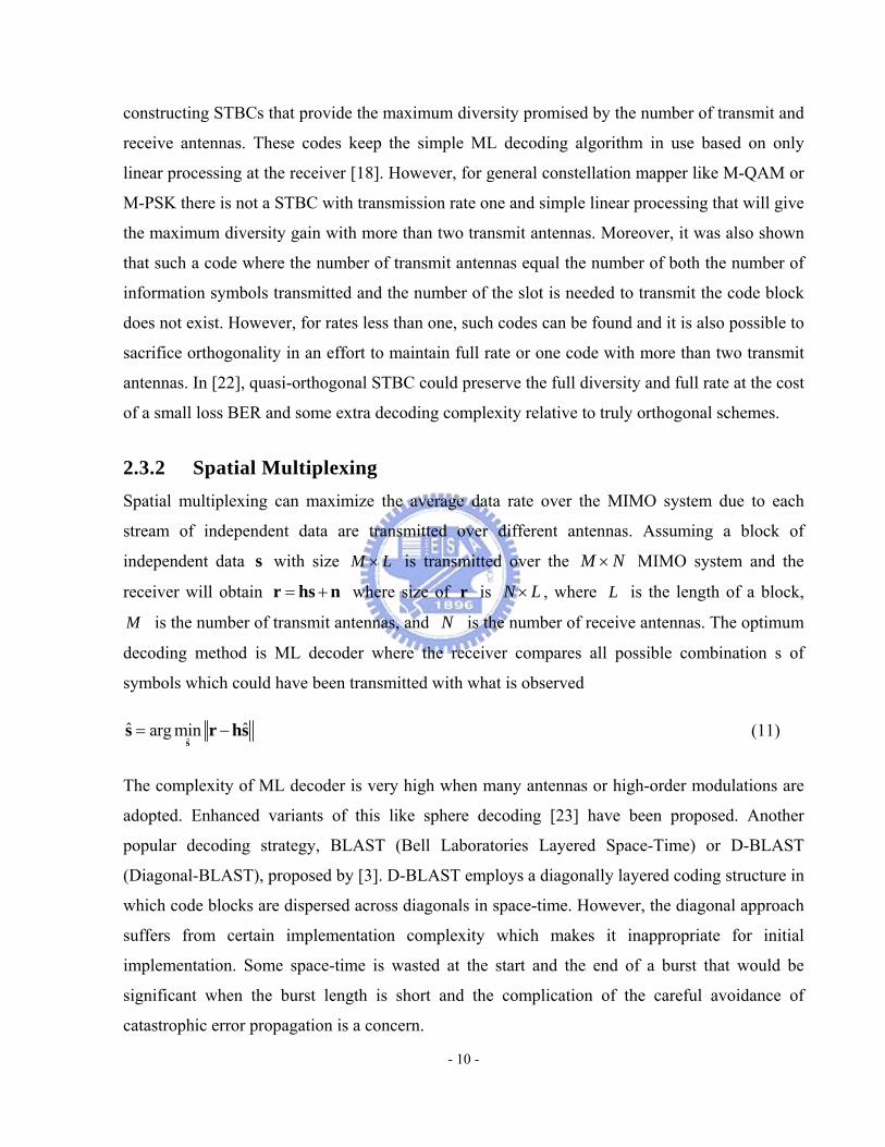
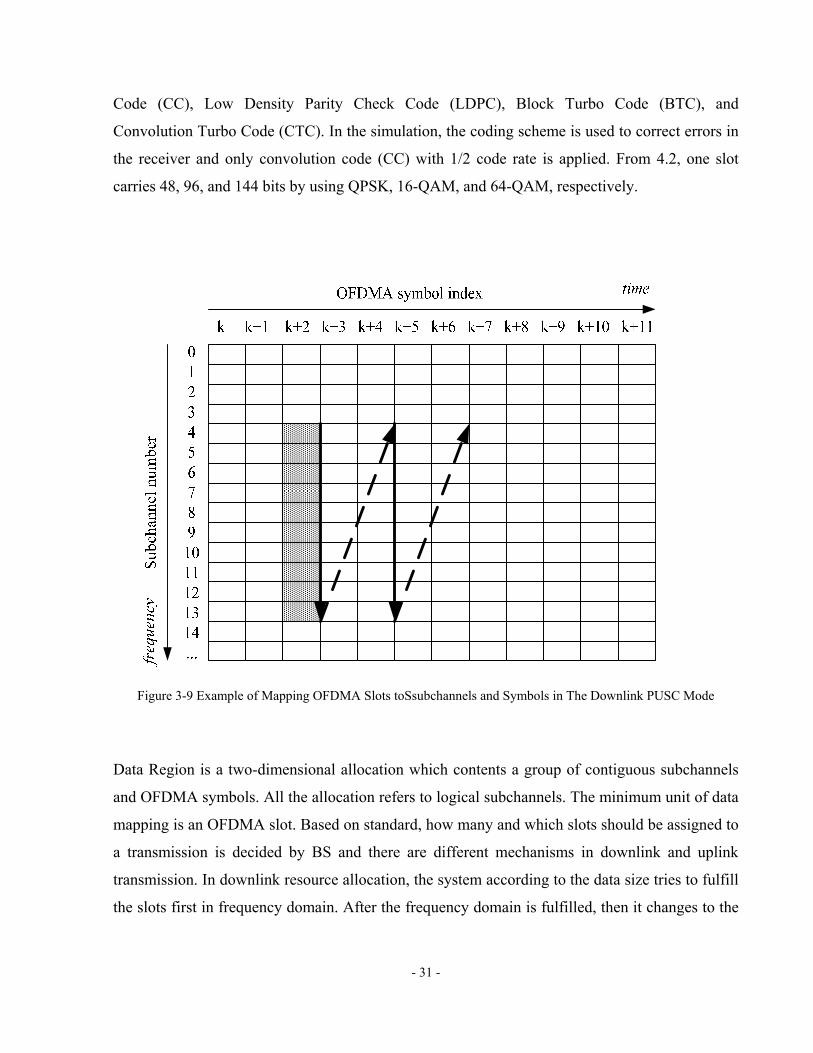
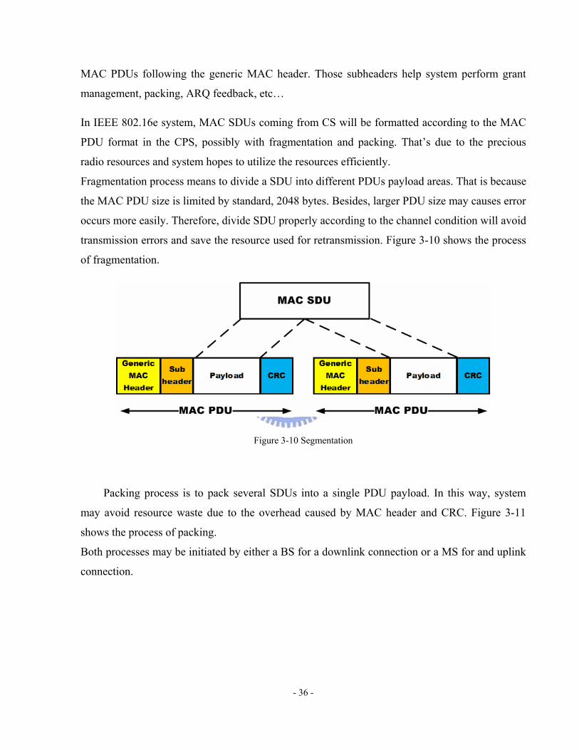
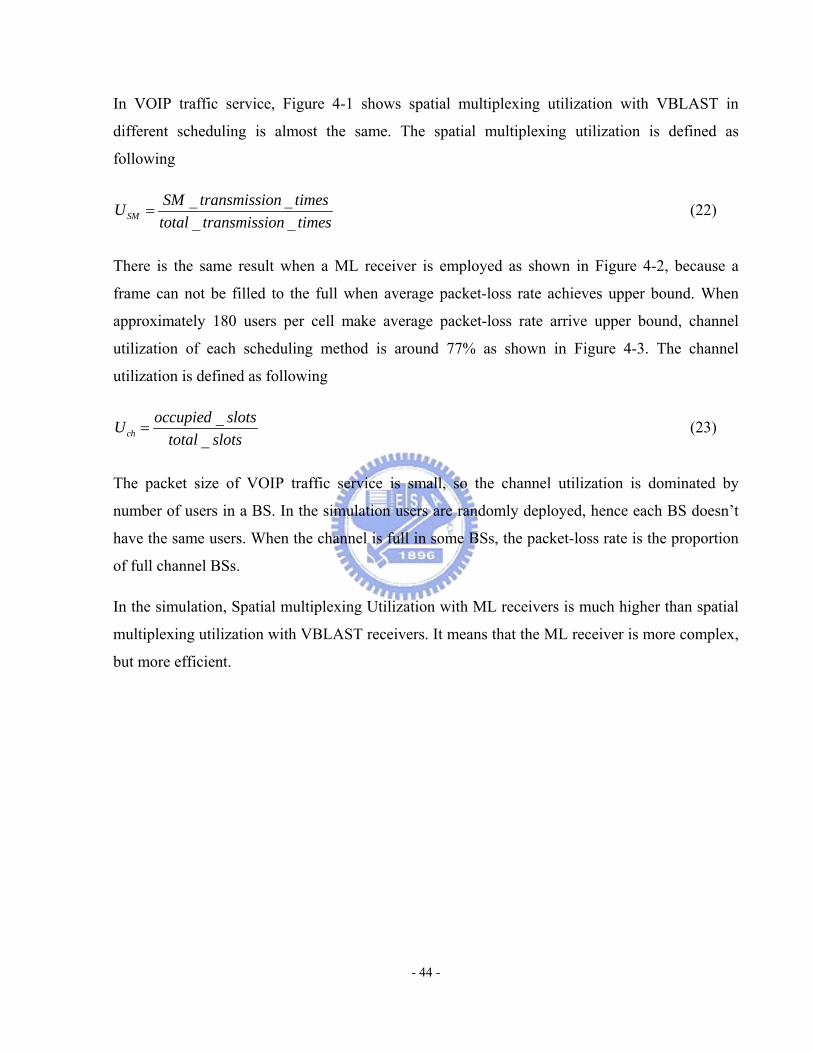
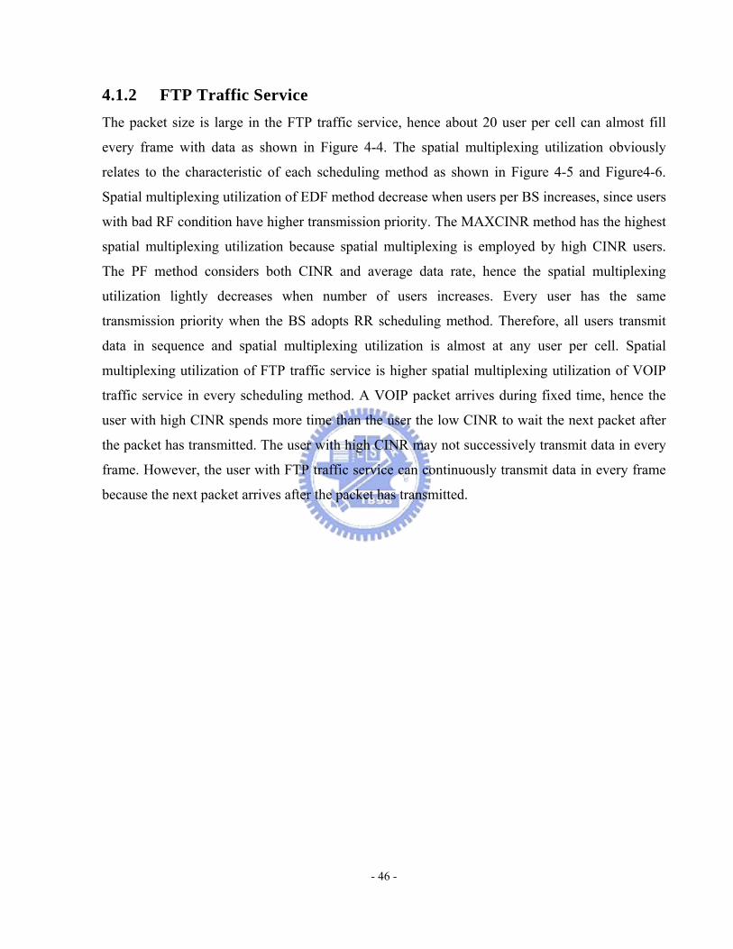
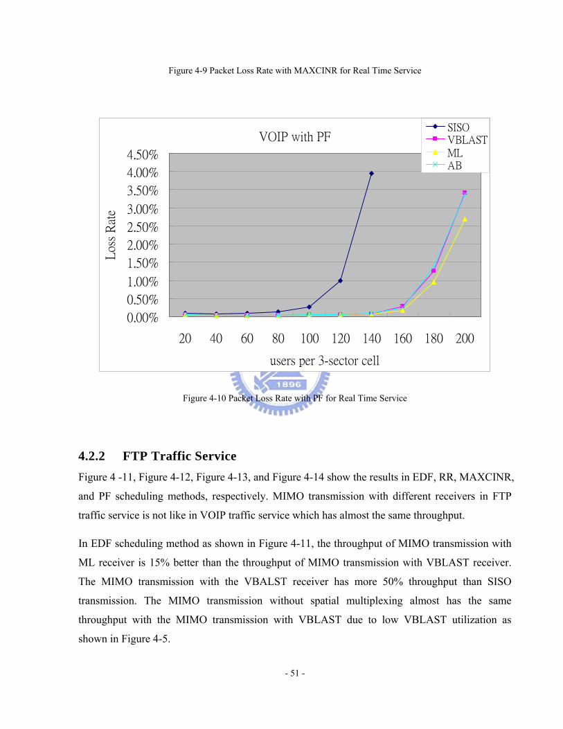

FTP with EDF
00
20
40
60
80
100
120
140
20 40 60 80 100 120
users per 3-sector cell
Uns
atis
fied
Min
imum
Rat
e
SISOVBLASTMLAB
Figure 4-11 Unsatisfied Minimum Rate with EDF for Non-real Time Service
In RR scheduling method as shown in Figure 4-12 the throughput of MIMO transmission with
ML receiver is 10 better than the throughput of MIMO transmission with VBLAST receiver
The MIMO transmission with the VBALST receiver has more 60 throughput than SISO
transmission The MIMO transmission without spatial multiplexing almost has the same
throughput with the MIMO transmission with VBLAST due to low VBLAST utilization as
shown in Figure 4-5
- 52 -
FTP with RR
00
20
40
60
80
100
120
20 40 60 80 100 120
users per 3-sector cell
Uns
atis
fied
Min
imum
Rat
e
SISOVBLASTMLAB
Figure 4-12 Unsatisfied Minimum Rate with RR for Non-real Time Service
In the MAXCINR scheduling method even MIMO transmission with the ML receiver can not
satisfy the QoS of FTP traffic service as shown in Figure 4-13 High CINR uses have high
priority to be served hence low CINR users donrsquot have a lot of probability to transmit data
- 53 -
FTP with MAXCINR
00
200
400
600
800
1000
20 40 60 80 100 120
users per 3-sector cell
Uns
atis
fied
Min
imum
Rat
e
SISOVBLASTMLAB
Figure 4-13 Unsatisfied Minimum Rate with MAXCINR for Non-real Time Service
In PF scheduling method as shown in Figure 4-14 the throughput of MIMO transmission with
ML receiver is 40 better than the throughput of MIMO transmission with VBLAST receiver
The MIMO transmission with the VBALST receiver has more 100 capacity than SISO
transmission The MIMO transmission without spatial multiplexing has less 10 throughput than
the MIMO transmission with VBLAST
- 54 -
FTP with PF
00
50
100
150
200
250
300
20 40 60 80 100 120
users per 3-sector cell
Uns
atis
fied
Min
imum
Rat
eSISOVBLASTMLAB
Figure 4-14 Unsatisfied Minimum Rate with PF for Non-real Time Service
The capacity in the PF scheduling method can be improved more than in EDF and RR scheduling
methods because the transmission rate is considered in the PF scheduling method
43 Throughput of FTP Traffic Service In the section the MAC throughput performance in downlink transmission with MIMO
technique is discussed in terms of different scheduling algorithms and different receiver
technique MAC throughput indicates the real data that have been transmitted It ignores the
header and the retransmitted data and reflects the real data which is really useful
In EDF scheduling method as shown in Figure 4-11 the throughput of MIMO transmission with
ML receiver is 15 better than the throughput of MIMO transmission with VBLAST receiver
The MIMO transmission with the VBALST receiver has more 50 throughput than SISO
transmission The MIMO transmission without spatial multiplexing almost has the same
- 55 -
throughput with the MIMO transmission with VBLAST due to low VBLAST utilization as
shown in Figure 4-5
FTP with EDF
0
5
10
15
20
25
20 40 60 80 100 120
users per 3-sector cell
Thr
ough
put
(Mbp
s
Cel
l)
SISOVBLASTMLAB
Figure 4-15 Throughput with EDF
In RR scheduling method as shown in Figure 4-12 the throughput of MIMO transmission with
ML receiver is 6 better than the throughput of MIMO transmission with VBLAST receiver
The MIMO transmission with the VBALST receiver has more 40 throughput than SISO
transmission The MIMO transmission without spatial multiplexing almost has the same
throughput with the MIMO transmission with VBLAST due to low VBLAST utilization as
shown in Figure 4-5
- 56 -
FTP with RR
0
2
4
6
8
10
12
14
16
20 40 60 80 100 120
users per 3-sector cell
Thr
ough
put
(Mbp
s
Cel
l)SISOVBLASTMLAB
Figure 4-16 Throughput with RR
In MAXCINR scheduling method as shown in Figure 4-17 the throughput of MIMO
transmission with ML receiver is 55 better than the throughput of MIMO transmission with
VBLAST receiver The MIMO transmission with the VBALST receiver has more 100
throughput than SISO transmission The MIMO transmission without spatial multiplexing has
less 20 throughput than the MIMO transmission with VBLAST
- 57 -
FTP with MAXCINR
0
5
10
15
20
25
30
35
40
20 40 60 80 100 120
users per 3-sector cell
Thr
ough
put
(Mbp
s
Cel
l)
SISOVBLASTMLAB
Figure 4-17 Throughput with MAXCINR
In PF scheduling method as shown in Figure 4-18 the throughput of MIMO transmission with
ML receiver is 45 better than the throughput of MIMO transmission with VBLAST receiver
The MIMO transmission with the VBALST receiver has more 100 throughput than SISO
transmission The MIMO transmission without spatial multiplexing has less 5 throughput than
the MIMO transmission with VBLAST
- 58 -
FTP with PF
0
5
10
15
20
25
30
20 40 60 80 100 120
users per 3-sector cell
Thr
ough
put
(Mbp
s
Cel
l)
SISOVBLASTMLAB
Figure 4-18 Throughput with PF
The throughput in MAXCINR and PF scheduling methods can be improved more than in EDF
and RR scheduling methods because the transmission rate is considered in MAXCINR and PF
scheduling methods
44 Fragmentation In Figure 4-19 the channel utilization decreases when users increase in a cell since high
transmission rate may causes large padding of a burst A VOIP packet is much smaller than a
FTP packet hence the padding is more serious in VOIP traffic Exploiting padding of a burst to
adapt PDU size can reduce loss rate as shown in Figure 4-20 When users per cell increase more
loss rate can be improved There is ARQ in the simulation so PDU can be retransmitted to
reduce PER When more users stay in a cell a PDU may not be retransmitted before its delay
bound loss rate be improved obviously
- 59 -
FTP with MaxCINR
954
956
958
960
962
964
966
968
40 60 80 100 120
users per 3-sector cell
Cha
nnel
Uti
liza
tion
ML
Figure 4-19 Channel Utilization for FTP Traffic Service
VOIP with PF
00
20
40
60
80
100
120
20 40 60 80 100 120 140 160 180 200
users per 3-sector cell
Los
s Im
prov
ed R
ate
SISO
VBLASTML
AB
Figure 4-20 Improved Loss Rate in PF Scheduling Method for VOIP Traffic Service
- 60 -
Chapter 5 Conclusion and Future Work
In the thesis our contributions are the system level platform establishment of MAC layer with
MIMO technique in WiMAX standard and the performance study of MIMO transmission system
First the MAC layer with MIMO technique in IEEE 80216e system is implemented in our study
The platform is used for preliminary understanding of MIMO system Secondly utilization of
different receivers of spatial multiplexing technique in different scheduling methods is studied
Then QoS of the MIMO System with different receivers in different scheduling methods is
studied Finally the characteristic of MIMO transmission is studied and a simple fragmentation
method is applied for improving the PER
From the performance simulation we can get the conclusion as below For real time service the
VBLAST utilization of different scheduling methods is the same and the spatial multiplexing
with the ML receiver utilization of different scheduling methods is also the same Furthermore
MAXCINR and PF scheduling methods can improve more QoS than RR and EDF scheduling
methods but it is not obvious It means that there is not a scheduling method with MIMO
technique which is more appropriate than others for real time service For non-real time service
the MAXCINR scheduling method has the highest spatial multiplexing utilization and the PF
scheduling method is better than EDF and RR scheduling methods However MAXCINR is not
the most appropriate scheduling method for non-real time service because MAXCINR can not
satisfy QoS The PF scheduling method can improve more QoS and provide higher throughput
than EDF and RR scheduling methods because it considers the transmission rate Therefore the
PF is most appropriate scheduling method for non-real time service When the transmission rate
is higher the influence of the padding of a burst is more serious
The MIMO system with mixed transmit diversity and spatial multiplexing almost has the same
capacity as the MIMO system only with transmit diversity for VOIP traffic service It means that
spatial multiplexing can provide high transmission rate but is not suitable for VOIP traffic
service
In the future work we can update to the channel model the other simple radio resource
management control algorithm in the platform which is referred to power control ARQ and
- 61 -
handoff algorithm With more advance radio resource management control algorithms the
performance can be upgraded more and QoS of can be guarantee further
- 62 -
Reference
[1] IEEE ldquoIEEE Standard for Local and Metropolitan Area Networks Part 16 Air Interface
for Fixed Broadband Wireless Access Systemsrdquo IEEE Std 80216-2004 (Revision of IEEE
Std 80216-2001) pp 1-857 2004
[2] IEEE ldquoIEEE Standard for Local and metropolitan area networks Part 16 Air Interface for
Fixed and Mobile Broadband Wireless Access Systems Amendment 2 Physical and
Medium Access Control Layers for Combined Fixed and Mobile Operation in Licensed
Bands and Corrigendum 1rdquo IEEE Std 80216e-2005 and IEEE Std 80216-2004Cor
1-2005 (Amendment and Corrigendum to IEEE Std 80216-2004) pp 1-822 2006
[3] G J Foschini ldquoLayered spacendashtime architecture for wireless communication in a fading
environment when using multielement antennasrdquo Bell Labs Tech J pp 41ndash59 Autumn
1996
[4] G J Foschini and M J Gans ldquoOn limits of wireless communications in a fading
environment when using multiple antennasrdquo Wireless Pers Commun vol 6 pp
311ndash335 Mar 1998
[5] E Telatar ldquoCapacity of multiantenna Gaussian channelsrdquo ATampT Bell Laboratories Tech
Memo June 1995
[6] G Raleigh and J M Cioffi ldquoSpatial-temporal coding for wireless communicationsrdquo
IEEE Trans Commun vol 46 pp 357ndash366 1998
[7] H Boumllcskei D Gesbert and A J Paulraj ldquoOn the capacity of OFDM-based spatial
multiplexing systemsrdquo IEEE Trans Commun vol 50 pp225ndash234 Feb 2002
[8] M S Lin ldquoRadio Resource Management in Mobile WiMAX Systemrdquo a thesis submitted
to NCTU EE pp 1-81 Jun 2006
[9] F Wang A Ghosh C Sankaran and S Benes ldquoWiMAX System Performance with
Multiple Transmit and Multiple Receive Antennasrdquo in IEEE Vehicular Technology Conf
pp 2807-2811 Apr 2007
- 63 -
[10] D Gerlach and AJ Paulraj ldquoAdaptive transmitting antenna arrays with feedbackrdquo IEEE
Signal Processing Letters vol1 pp150-152 Oct 1994
[11] JH Winters ldquo Switched diversity for feedback with DPSK mobile radio systemsrdquo IEEE
Trans Veh Technol volVT-32 pp 134-150 Feb 1983
[12] RW Heath Jr S Sandhu and A J Paulraj ldquo Antenna selection for spatial multiplexing
systems with linear receiversrdquo IEEE Commun Lett vol5 pp 142-144 Apr 2001
[13] RS Blum and JW Winters ldquoOn optimum MIMO with antenna selectionrdquo IEEE Int
Conf Commun vol1 pp386-390 May 2002
[14] N Seshadri and J H Winters ldquoTwo schemes for improving the performance of
frequency-division duplex (FDD) transmission systems using transmitter antenna
diversityrdquo Int J Wireless Inform Networks vol 1 pp 49ndash60 Jan 1994
A Wittneben ldquoA new bandwidth efficient transmit antenna modulation diversity scheme
for linear digital modulationrdquo in Proc IEEE ICC vol 3 pp 1630ndash1634 1993
[15] VTarokh N Sesahdri and A R Calderbank ldquoSpace-Time codes for high data rate
wireless communication Performance criterion and code constructionrdquo IEEE Trans
Inform Theory vol44 pp744-765 Mar 1998
[16] V Tarokh H Jafarkhani and A R Calderbank ldquoSpace-Time Block codes from
orthogonal designsrdquo IEEE Trans Inform Theory vol45 pp1456-1467 Jul 1999
[17] S M Alamouti ldquoA simple transmit diversity technique for wireless communicationsrdquo
IEEE J Select Areas Commun vol16 pp 1451-1458 Oct 1998
[18] V Tarokh H Jafarkhani and A R Calderbank ldquoSpacendashtime block codes for wireless
communications Performance resultsrdquo IEEE J Select Areas Commun vol 17 pp
451ndash460 Mar 1999
[19] G Ganesan and P Stoica ldquoSpacendashtime diversity using orthogonal and amicable
orthogonal designsrdquo Wireless Pers Commun vol 18 pp 165ndash178 Aug 2001
- 64 -
[20] H Jafarkhani ldquoA quasi orthogonal space time block coderdquo IEEE Trans Commun vol
49 pp 1ndash4 Jan 2001
[21] Tirkkonen A Boariu and A Hottinen ldquoMinimal nonorthogonality rate 1 spacendashtime
block code for 3+ tx antennasrdquo in Proc IEEE Int Symp Spread Spectrum Technol pp
429ndash432 2000
[22] M O Damen A Chkeif and J C Belfiore ldquoLattice codes decoder for spacendashtime
codesrdquo IEEE Commun Lett vol 4 pp 161ndash163 May 2000
[23] P W Wolnainsky G J Foschini G D Golden and R A Valenzuela ldquoV-BLAST An
architecture for realizing very high data rates over the rich-scattering wireless channelrdquo in
Proc ISSSE pp 295-300 1998
[24] Mobile WiMAX ndash Part 1 A Technical Overview and Performance Evalutionrdquo in WiMAX
Forum pp 1-53 Jun 2006
[25] Mobile WiMAX ndash Part 2 A Comparative Analysisrdquo in WiMAX Forum pp 1-47 May
2006
[26] 3GPP ldquo3rd Generation Partnership Project Technical Specification Group Radio Access
Network Spatial channel model for Multiple Input Multiple Output (MIMO) simulations
(Release 7)rdquo 3GPP TR 25996 pp 1-40 Jun 2007
[27] M Gudmundson ldquoCorrelation Model for Shadow Fading in Mobile Radio Systemsrdquo
Elect Lett Vol 27 pp 2145-2146 Nov 1991
[28] C Wengerter J Ohohorst and AGE von Elbwart ldquoFairness and throughput analysis for
generalized proportional fair frequency scheduling in OFDMArdquo IEEE Veh Technol
Conf Vol 3 pp1903-1907 2005
[29] S Yoon Y Cho C B Chae and H Lee ldquoSystem level performance of OFDMA
forward link with proportional fair schedulingrdquo IEEE Int Symp Pers Indoor and Moblie
Radio Commun Vol 2 pp 1384-1388 Sep 2004
- 65 -
[30] S Ryu B Ryu H Seo and M Shin ldquo Urgency and Efficiency Based Packet Scheduling
Algorithm for OFDMA Wireless Systemrdquo IEEE Int Commun Conf Vol 4 pp
2779-2785 May 2005
[31] F M Chiussi and V Sivaraman ldquoAchieving high utilization in guaranteed services
networks using early-deadline-first schedulingrdquo in Proc IEEE IWQoS pp 209-217 May
1998
A Gyasi-Agyei ldquoMultiuser Diversity Based Opportunistic Scheduling for Wireless Data
Networksrdquo IEEE Commun Lett Vol 9 pp 670-672 Jul 2005
B J Chian ldquoQos-based Opportunistic Scheduling Algorithm for Mixed-traffic
Environmentrdquo A Thesis Submitted to NCTU EE pp 1-81 Jun 2007
[32] 3GPP2 ldquocdma2000 Evaluation Methodology Revision 0rdquo 3GPP2 C R 1002-0 pp1-194
Dec 2004
[33] ldquo3G amp The Future of Wirelessrdquo PDAs amp Cell Phones Vol 8 pp 48-51 May 2002
[34] ITU-T ldquoCoding of Speech at 8 kbits Using Conjugate-structure Algebraic-code-excited
Linear-predictionrdquo ITU-T Recommendation G729 pp 1-39 Mar 1996
- 66 -

FTP with RR
00
20
40
60
80
100
120
20 40 60 80 100 120
users per 3-sector cell
Uns
atis
fied
Min
imum
Rat
e
SISOVBLASTMLAB
Figure 4-12 Unsatisfied Minimum Rate with RR for Non-real Time Service
In the MAXCINR scheduling method even MIMO transmission with the ML receiver can not
satisfy the QoS of FTP traffic service as shown in Figure 4-13 High CINR uses have high
priority to be served hence low CINR users donrsquot have a lot of probability to transmit data
- 53 -
FTP with MAXCINR
00
200
400
600
800
1000
20 40 60 80 100 120
users per 3-sector cell
Uns
atis
fied
Min
imum
Rat
e
SISOVBLASTMLAB
Figure 4-13 Unsatisfied Minimum Rate with MAXCINR for Non-real Time Service
In PF scheduling method as shown in Figure 4-14 the throughput of MIMO transmission with
ML receiver is 40 better than the throughput of MIMO transmission with VBLAST receiver
The MIMO transmission with the VBALST receiver has more 100 capacity than SISO
transmission The MIMO transmission without spatial multiplexing has less 10 throughput than
the MIMO transmission with VBLAST
- 54 -
FTP with PF
00
50
100
150
200
250
300
20 40 60 80 100 120
users per 3-sector cell
Uns
atis
fied
Min
imum
Rat
eSISOVBLASTMLAB
Figure 4-14 Unsatisfied Minimum Rate with PF for Non-real Time Service
The capacity in the PF scheduling method can be improved more than in EDF and RR scheduling
methods because the transmission rate is considered in the PF scheduling method
43 Throughput of FTP Traffic Service In the section the MAC throughput performance in downlink transmission with MIMO
technique is discussed in terms of different scheduling algorithms and different receiver
technique MAC throughput indicates the real data that have been transmitted It ignores the
header and the retransmitted data and reflects the real data which is really useful
In EDF scheduling method as shown in Figure 4-11 the throughput of MIMO transmission with
ML receiver is 15 better than the throughput of MIMO transmission with VBLAST receiver
The MIMO transmission with the VBALST receiver has more 50 throughput than SISO
transmission The MIMO transmission without spatial multiplexing almost has the same
- 55 -
throughput with the MIMO transmission with VBLAST due to low VBLAST utilization as
shown in Figure 4-5
FTP with EDF
0
5
10
15
20
25
20 40 60 80 100 120
users per 3-sector cell
Thr
ough
put
(Mbp
s
Cel
l)
SISOVBLASTMLAB
Figure 4-15 Throughput with EDF
In RR scheduling method as shown in Figure 4-12 the throughput of MIMO transmission with
ML receiver is 6 better than the throughput of MIMO transmission with VBLAST receiver
The MIMO transmission with the VBALST receiver has more 40 throughput than SISO
transmission The MIMO transmission without spatial multiplexing almost has the same
throughput with the MIMO transmission with VBLAST due to low VBLAST utilization as
shown in Figure 4-5
- 56 -
FTP with RR
0
2
4
6
8
10
12
14
16
20 40 60 80 100 120
users per 3-sector cell
Thr
ough
put
(Mbp
s
Cel
l)SISOVBLASTMLAB
Figure 4-16 Throughput with RR
In MAXCINR scheduling method as shown in Figure 4-17 the throughput of MIMO
transmission with ML receiver is 55 better than the throughput of MIMO transmission with
VBLAST receiver The MIMO transmission with the VBALST receiver has more 100
throughput than SISO transmission The MIMO transmission without spatial multiplexing has
less 20 throughput than the MIMO transmission with VBLAST
- 57 -
FTP with MAXCINR
0
5
10
15
20
25
30
35
40
20 40 60 80 100 120
users per 3-sector cell
Thr
ough
put
(Mbp
s
Cel
l)
SISOVBLASTMLAB
Figure 4-17 Throughput with MAXCINR
In PF scheduling method as shown in Figure 4-18 the throughput of MIMO transmission with
ML receiver is 45 better than the throughput of MIMO transmission with VBLAST receiver
The MIMO transmission with the VBALST receiver has more 100 throughput than SISO
transmission The MIMO transmission without spatial multiplexing has less 5 throughput than
the MIMO transmission with VBLAST
- 58 -
FTP with PF
0
5
10
15
20
25
30
20 40 60 80 100 120
users per 3-sector cell
Thr
ough
put
(Mbp
s
Cel
l)
SISOVBLASTMLAB
Figure 4-18 Throughput with PF
The throughput in MAXCINR and PF scheduling methods can be improved more than in EDF
and RR scheduling methods because the transmission rate is considered in MAXCINR and PF
scheduling methods
44 Fragmentation In Figure 4-19 the channel utilization decreases when users increase in a cell since high
transmission rate may causes large padding of a burst A VOIP packet is much smaller than a
FTP packet hence the padding is more serious in VOIP traffic Exploiting padding of a burst to
adapt PDU size can reduce loss rate as shown in Figure 4-20 When users per cell increase more
loss rate can be improved There is ARQ in the simulation so PDU can be retransmitted to
reduce PER When more users stay in a cell a PDU may not be retransmitted before its delay
bound loss rate be improved obviously
- 59 -
FTP with MaxCINR
954
956
958
960
962
964
966
968
40 60 80 100 120
users per 3-sector cell
Cha
nnel
Uti
liza
tion
ML
Figure 4-19 Channel Utilization for FTP Traffic Service
VOIP with PF
00
20
40
60
80
100
120
20 40 60 80 100 120 140 160 180 200
users per 3-sector cell
Los
s Im
prov
ed R
ate
SISO
VBLASTML
AB
Figure 4-20 Improved Loss Rate in PF Scheduling Method for VOIP Traffic Service
- 60 -
Chapter 5 Conclusion and Future Work
In the thesis our contributions are the system level platform establishment of MAC layer with
MIMO technique in WiMAX standard and the performance study of MIMO transmission system
First the MAC layer with MIMO technique in IEEE 80216e system is implemented in our study
The platform is used for preliminary understanding of MIMO system Secondly utilization of
different receivers of spatial multiplexing technique in different scheduling methods is studied
Then QoS of the MIMO System with different receivers in different scheduling methods is
studied Finally the characteristic of MIMO transmission is studied and a simple fragmentation
method is applied for improving the PER
From the performance simulation we can get the conclusion as below For real time service the
VBLAST utilization of different scheduling methods is the same and the spatial multiplexing
with the ML receiver utilization of different scheduling methods is also the same Furthermore
MAXCINR and PF scheduling methods can improve more QoS than RR and EDF scheduling
methods but it is not obvious It means that there is not a scheduling method with MIMO
technique which is more appropriate than others for real time service For non-real time service
the MAXCINR scheduling method has the highest spatial multiplexing utilization and the PF
scheduling method is better than EDF and RR scheduling methods However MAXCINR is not
the most appropriate scheduling method for non-real time service because MAXCINR can not
satisfy QoS The PF scheduling method can improve more QoS and provide higher throughput
than EDF and RR scheduling methods because it considers the transmission rate Therefore the
PF is most appropriate scheduling method for non-real time service When the transmission rate
is higher the influence of the padding of a burst is more serious
The MIMO system with mixed transmit diversity and spatial multiplexing almost has the same
capacity as the MIMO system only with transmit diversity for VOIP traffic service It means that
spatial multiplexing can provide high transmission rate but is not suitable for VOIP traffic
service
In the future work we can update to the channel model the other simple radio resource
management control algorithm in the platform which is referred to power control ARQ and
- 61 -
handoff algorithm With more advance radio resource management control algorithms the
performance can be upgraded more and QoS of can be guarantee further
- 62 -
Reference
[1] IEEE ldquoIEEE Standard for Local and Metropolitan Area Networks Part 16 Air Interface
for Fixed Broadband Wireless Access Systemsrdquo IEEE Std 80216-2004 (Revision of IEEE
Std 80216-2001) pp 1-857 2004
[2] IEEE ldquoIEEE Standard for Local and metropolitan area networks Part 16 Air Interface for
Fixed and Mobile Broadband Wireless Access Systems Amendment 2 Physical and
Medium Access Control Layers for Combined Fixed and Mobile Operation in Licensed
Bands and Corrigendum 1rdquo IEEE Std 80216e-2005 and IEEE Std 80216-2004Cor
1-2005 (Amendment and Corrigendum to IEEE Std 80216-2004) pp 1-822 2006
[3] G J Foschini ldquoLayered spacendashtime architecture for wireless communication in a fading
environment when using multielement antennasrdquo Bell Labs Tech J pp 41ndash59 Autumn
1996
[4] G J Foschini and M J Gans ldquoOn limits of wireless communications in a fading
environment when using multiple antennasrdquo Wireless Pers Commun vol 6 pp
311ndash335 Mar 1998
[5] E Telatar ldquoCapacity of multiantenna Gaussian channelsrdquo ATampT Bell Laboratories Tech
Memo June 1995
[6] G Raleigh and J M Cioffi ldquoSpatial-temporal coding for wireless communicationsrdquo
IEEE Trans Commun vol 46 pp 357ndash366 1998
[7] H Boumllcskei D Gesbert and A J Paulraj ldquoOn the capacity of OFDM-based spatial
multiplexing systemsrdquo IEEE Trans Commun vol 50 pp225ndash234 Feb 2002
[8] M S Lin ldquoRadio Resource Management in Mobile WiMAX Systemrdquo a thesis submitted
to NCTU EE pp 1-81 Jun 2006
[9] F Wang A Ghosh C Sankaran and S Benes ldquoWiMAX System Performance with
Multiple Transmit and Multiple Receive Antennasrdquo in IEEE Vehicular Technology Conf
pp 2807-2811 Apr 2007
- 63 -
[10] D Gerlach and AJ Paulraj ldquoAdaptive transmitting antenna arrays with feedbackrdquo IEEE
Signal Processing Letters vol1 pp150-152 Oct 1994
[11] JH Winters ldquo Switched diversity for feedback with DPSK mobile radio systemsrdquo IEEE
Trans Veh Technol volVT-32 pp 134-150 Feb 1983
[12] RW Heath Jr S Sandhu and A J Paulraj ldquo Antenna selection for spatial multiplexing
systems with linear receiversrdquo IEEE Commun Lett vol5 pp 142-144 Apr 2001
[13] RS Blum and JW Winters ldquoOn optimum MIMO with antenna selectionrdquo IEEE Int
Conf Commun vol1 pp386-390 May 2002
[14] N Seshadri and J H Winters ldquoTwo schemes for improving the performance of
frequency-division duplex (FDD) transmission systems using transmitter antenna
diversityrdquo Int J Wireless Inform Networks vol 1 pp 49ndash60 Jan 1994
A Wittneben ldquoA new bandwidth efficient transmit antenna modulation diversity scheme
for linear digital modulationrdquo in Proc IEEE ICC vol 3 pp 1630ndash1634 1993
[15] VTarokh N Sesahdri and A R Calderbank ldquoSpace-Time codes for high data rate
wireless communication Performance criterion and code constructionrdquo IEEE Trans
Inform Theory vol44 pp744-765 Mar 1998
[16] V Tarokh H Jafarkhani and A R Calderbank ldquoSpace-Time Block codes from
orthogonal designsrdquo IEEE Trans Inform Theory vol45 pp1456-1467 Jul 1999
[17] S M Alamouti ldquoA simple transmit diversity technique for wireless communicationsrdquo
IEEE J Select Areas Commun vol16 pp 1451-1458 Oct 1998
[18] V Tarokh H Jafarkhani and A R Calderbank ldquoSpacendashtime block codes for wireless
communications Performance resultsrdquo IEEE J Select Areas Commun vol 17 pp
451ndash460 Mar 1999
[19] G Ganesan and P Stoica ldquoSpacendashtime diversity using orthogonal and amicable
orthogonal designsrdquo Wireless Pers Commun vol 18 pp 165ndash178 Aug 2001
- 64 -
[20] H Jafarkhani ldquoA quasi orthogonal space time block coderdquo IEEE Trans Commun vol
49 pp 1ndash4 Jan 2001
[21] Tirkkonen A Boariu and A Hottinen ldquoMinimal nonorthogonality rate 1 spacendashtime
block code for 3+ tx antennasrdquo in Proc IEEE Int Symp Spread Spectrum Technol pp
429ndash432 2000
[22] M O Damen A Chkeif and J C Belfiore ldquoLattice codes decoder for spacendashtime
codesrdquo IEEE Commun Lett vol 4 pp 161ndash163 May 2000
[23] P W Wolnainsky G J Foschini G D Golden and R A Valenzuela ldquoV-BLAST An
architecture for realizing very high data rates over the rich-scattering wireless channelrdquo in
Proc ISSSE pp 295-300 1998
[24] Mobile WiMAX ndash Part 1 A Technical Overview and Performance Evalutionrdquo in WiMAX
Forum pp 1-53 Jun 2006
[25] Mobile WiMAX ndash Part 2 A Comparative Analysisrdquo in WiMAX Forum pp 1-47 May
2006
[26] 3GPP ldquo3rd Generation Partnership Project Technical Specification Group Radio Access
Network Spatial channel model for Multiple Input Multiple Output (MIMO) simulations
(Release 7)rdquo 3GPP TR 25996 pp 1-40 Jun 2007
[27] M Gudmundson ldquoCorrelation Model for Shadow Fading in Mobile Radio Systemsrdquo
Elect Lett Vol 27 pp 2145-2146 Nov 1991
[28] C Wengerter J Ohohorst and AGE von Elbwart ldquoFairness and throughput analysis for
generalized proportional fair frequency scheduling in OFDMArdquo IEEE Veh Technol
Conf Vol 3 pp1903-1907 2005
[29] S Yoon Y Cho C B Chae and H Lee ldquoSystem level performance of OFDMA
forward link with proportional fair schedulingrdquo IEEE Int Symp Pers Indoor and Moblie
Radio Commun Vol 2 pp 1384-1388 Sep 2004
- 65 -
[30] S Ryu B Ryu H Seo and M Shin ldquo Urgency and Efficiency Based Packet Scheduling
Algorithm for OFDMA Wireless Systemrdquo IEEE Int Commun Conf Vol 4 pp
2779-2785 May 2005
[31] F M Chiussi and V Sivaraman ldquoAchieving high utilization in guaranteed services
networks using early-deadline-first schedulingrdquo in Proc IEEE IWQoS pp 209-217 May
1998
A Gyasi-Agyei ldquoMultiuser Diversity Based Opportunistic Scheduling for Wireless Data
Networksrdquo IEEE Commun Lett Vol 9 pp 670-672 Jul 2005
B J Chian ldquoQos-based Opportunistic Scheduling Algorithm for Mixed-traffic
Environmentrdquo A Thesis Submitted to NCTU EE pp 1-81 Jun 2007
[32] 3GPP2 ldquocdma2000 Evaluation Methodology Revision 0rdquo 3GPP2 C R 1002-0 pp1-194
Dec 2004
[33] ldquo3G amp The Future of Wirelessrdquo PDAs amp Cell Phones Vol 8 pp 48-51 May 2002
[34] ITU-T ldquoCoding of Speech at 8 kbits Using Conjugate-structure Algebraic-code-excited
Linear-predictionrdquo ITU-T Recommendation G729 pp 1-39 Mar 1996
- 66 -
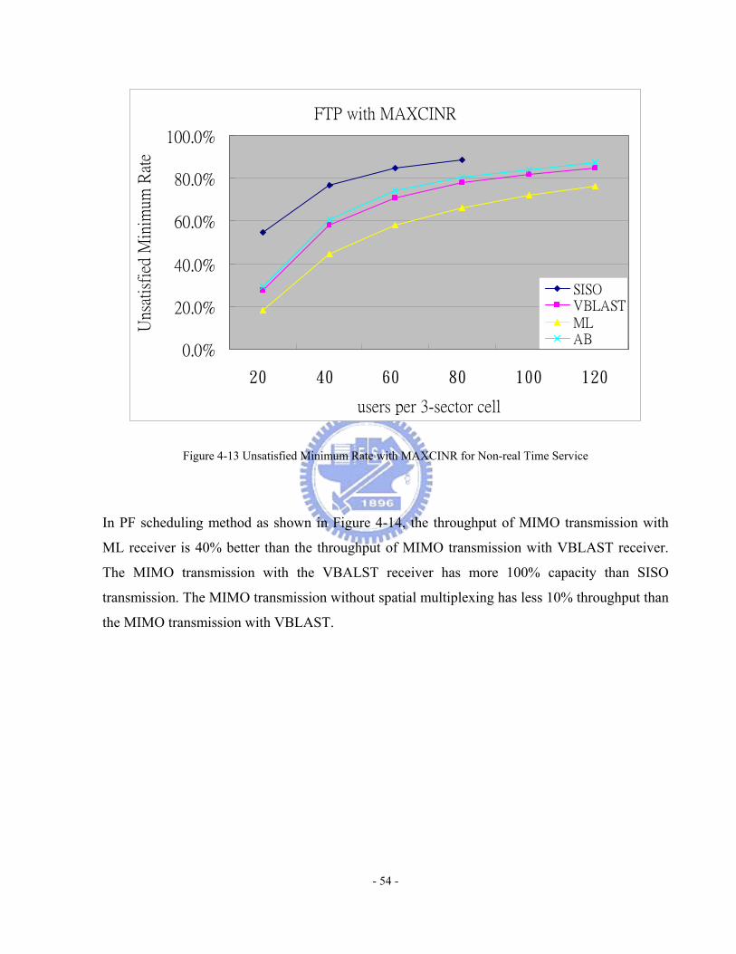
FTP with MAXCINR
00
200
400
600
800
1000
20 40 60 80 100 120
users per 3-sector cell
Uns
atis
fied
Min
imum
Rat
e
SISOVBLASTMLAB
Figure 4-13 Unsatisfied Minimum Rate with MAXCINR for Non-real Time Service
In PF scheduling method as shown in Figure 4-14 the throughput of MIMO transmission with
ML receiver is 40 better than the throughput of MIMO transmission with VBLAST receiver
The MIMO transmission with the VBALST receiver has more 100 capacity than SISO
transmission The MIMO transmission without spatial multiplexing has less 10 throughput than
the MIMO transmission with VBLAST
- 54 -
FTP with PF
00
50
100
150
200
250
300
20 40 60 80 100 120
users per 3-sector cell
Uns
atis
fied
Min
imum
Rat
eSISOVBLASTMLAB
Figure 4-14 Unsatisfied Minimum Rate with PF for Non-real Time Service
The capacity in the PF scheduling method can be improved more than in EDF and RR scheduling
methods because the transmission rate is considered in the PF scheduling method
43 Throughput of FTP Traffic Service In the section the MAC throughput performance in downlink transmission with MIMO
technique is discussed in terms of different scheduling algorithms and different receiver
technique MAC throughput indicates the real data that have been transmitted It ignores the
header and the retransmitted data and reflects the real data which is really useful
In EDF scheduling method as shown in Figure 4-11 the throughput of MIMO transmission with
ML receiver is 15 better than the throughput of MIMO transmission with VBLAST receiver
The MIMO transmission with the VBALST receiver has more 50 throughput than SISO
transmission The MIMO transmission without spatial multiplexing almost has the same
- 55 -
throughput with the MIMO transmission with VBLAST due to low VBLAST utilization as
shown in Figure 4-5
FTP with EDF
0
5
10
15
20
25
20 40 60 80 100 120
users per 3-sector cell
Thr
ough
put
(Mbp
s
Cel
l)
SISOVBLASTMLAB
Figure 4-15 Throughput with EDF
In RR scheduling method as shown in Figure 4-12 the throughput of MIMO transmission with
ML receiver is 6 better than the throughput of MIMO transmission with VBLAST receiver
The MIMO transmission with the VBALST receiver has more 40 throughput than SISO
transmission The MIMO transmission without spatial multiplexing almost has the same
throughput with the MIMO transmission with VBLAST due to low VBLAST utilization as
shown in Figure 4-5
- 56 -
FTP with RR
0
2
4
6
8
10
12
14
16
20 40 60 80 100 120
users per 3-sector cell
Thr
ough
put
(Mbp
s
Cel
l)SISOVBLASTMLAB
Figure 4-16 Throughput with RR
In MAXCINR scheduling method as shown in Figure 4-17 the throughput of MIMO
transmission with ML receiver is 55 better than the throughput of MIMO transmission with
VBLAST receiver The MIMO transmission with the VBALST receiver has more 100
throughput than SISO transmission The MIMO transmission without spatial multiplexing has
less 20 throughput than the MIMO transmission with VBLAST
- 57 -
FTP with MAXCINR
0
5
10
15
20
25
30
35
40
20 40 60 80 100 120
users per 3-sector cell
Thr
ough
put
(Mbp
s
Cel
l)
SISOVBLASTMLAB
Figure 4-17 Throughput with MAXCINR
In PF scheduling method as shown in Figure 4-18 the throughput of MIMO transmission with
ML receiver is 45 better than the throughput of MIMO transmission with VBLAST receiver
The MIMO transmission with the VBALST receiver has more 100 throughput than SISO
transmission The MIMO transmission without spatial multiplexing has less 5 throughput than
the MIMO transmission with VBLAST
- 58 -
FTP with PF
0
5
10
15
20
25
30
20 40 60 80 100 120
users per 3-sector cell
Thr
ough
put
(Mbp
s
Cel
l)
SISOVBLASTMLAB
Figure 4-18 Throughput with PF
The throughput in MAXCINR and PF scheduling methods can be improved more than in EDF
and RR scheduling methods because the transmission rate is considered in MAXCINR and PF
scheduling methods
44 Fragmentation In Figure 4-19 the channel utilization decreases when users increase in a cell since high
transmission rate may causes large padding of a burst A VOIP packet is much smaller than a
FTP packet hence the padding is more serious in VOIP traffic Exploiting padding of a burst to
adapt PDU size can reduce loss rate as shown in Figure 4-20 When users per cell increase more
loss rate can be improved There is ARQ in the simulation so PDU can be retransmitted to
reduce PER When more users stay in a cell a PDU may not be retransmitted before its delay
bound loss rate be improved obviously
- 59 -
FTP with MaxCINR
954
956
958
960
962
964
966
968
40 60 80 100 120
users per 3-sector cell
Cha
nnel
Uti
liza
tion
ML
Figure 4-19 Channel Utilization for FTP Traffic Service
VOIP with PF
00
20
40
60
80
100
120
20 40 60 80 100 120 140 160 180 200
users per 3-sector cell
Los
s Im
prov
ed R
ate
SISO
VBLASTML
AB
Figure 4-20 Improved Loss Rate in PF Scheduling Method for VOIP Traffic Service
- 60 -
Chapter 5 Conclusion and Future Work
In the thesis our contributions are the system level platform establishment of MAC layer with
MIMO technique in WiMAX standard and the performance study of MIMO transmission system
First the MAC layer with MIMO technique in IEEE 80216e system is implemented in our study
The platform is used for preliminary understanding of MIMO system Secondly utilization of
different receivers of spatial multiplexing technique in different scheduling methods is studied
Then QoS of the MIMO System with different receivers in different scheduling methods is
studied Finally the characteristic of MIMO transmission is studied and a simple fragmentation
method is applied for improving the PER
From the performance simulation we can get the conclusion as below For real time service the
VBLAST utilization of different scheduling methods is the same and the spatial multiplexing
with the ML receiver utilization of different scheduling methods is also the same Furthermore
MAXCINR and PF scheduling methods can improve more QoS than RR and EDF scheduling
methods but it is not obvious It means that there is not a scheduling method with MIMO
technique which is more appropriate than others for real time service For non-real time service
the MAXCINR scheduling method has the highest spatial multiplexing utilization and the PF
scheduling method is better than EDF and RR scheduling methods However MAXCINR is not
the most appropriate scheduling method for non-real time service because MAXCINR can not
satisfy QoS The PF scheduling method can improve more QoS and provide higher throughput
than EDF and RR scheduling methods because it considers the transmission rate Therefore the
PF is most appropriate scheduling method for non-real time service When the transmission rate
is higher the influence of the padding of a burst is more serious
The MIMO system with mixed transmit diversity and spatial multiplexing almost has the same
capacity as the MIMO system only with transmit diversity for VOIP traffic service It means that
spatial multiplexing can provide high transmission rate but is not suitable for VOIP traffic
service
In the future work we can update to the channel model the other simple radio resource
management control algorithm in the platform which is referred to power control ARQ and
- 61 -
handoff algorithm With more advance radio resource management control algorithms the
performance can be upgraded more and QoS of can be guarantee further
- 62 -
Reference
[1] IEEE ldquoIEEE Standard for Local and Metropolitan Area Networks Part 16 Air Interface
for Fixed Broadband Wireless Access Systemsrdquo IEEE Std 80216-2004 (Revision of IEEE
Std 80216-2001) pp 1-857 2004
[2] IEEE ldquoIEEE Standard for Local and metropolitan area networks Part 16 Air Interface for
Fixed and Mobile Broadband Wireless Access Systems Amendment 2 Physical and
Medium Access Control Layers for Combined Fixed and Mobile Operation in Licensed
Bands and Corrigendum 1rdquo IEEE Std 80216e-2005 and IEEE Std 80216-2004Cor
1-2005 (Amendment and Corrigendum to IEEE Std 80216-2004) pp 1-822 2006
[3] G J Foschini ldquoLayered spacendashtime architecture for wireless communication in a fading
environment when using multielement antennasrdquo Bell Labs Tech J pp 41ndash59 Autumn
1996
[4] G J Foschini and M J Gans ldquoOn limits of wireless communications in a fading
environment when using multiple antennasrdquo Wireless Pers Commun vol 6 pp
311ndash335 Mar 1998
[5] E Telatar ldquoCapacity of multiantenna Gaussian channelsrdquo ATampT Bell Laboratories Tech
Memo June 1995
[6] G Raleigh and J M Cioffi ldquoSpatial-temporal coding for wireless communicationsrdquo
IEEE Trans Commun vol 46 pp 357ndash366 1998
[7] H Boumllcskei D Gesbert and A J Paulraj ldquoOn the capacity of OFDM-based spatial
multiplexing systemsrdquo IEEE Trans Commun vol 50 pp225ndash234 Feb 2002
[8] M S Lin ldquoRadio Resource Management in Mobile WiMAX Systemrdquo a thesis submitted
to NCTU EE pp 1-81 Jun 2006
[9] F Wang A Ghosh C Sankaran and S Benes ldquoWiMAX System Performance with
Multiple Transmit and Multiple Receive Antennasrdquo in IEEE Vehicular Technology Conf
pp 2807-2811 Apr 2007
- 63 -
[10] D Gerlach and AJ Paulraj ldquoAdaptive transmitting antenna arrays with feedbackrdquo IEEE
Signal Processing Letters vol1 pp150-152 Oct 1994
[11] JH Winters ldquo Switched diversity for feedback with DPSK mobile radio systemsrdquo IEEE
Trans Veh Technol volVT-32 pp 134-150 Feb 1983
[12] RW Heath Jr S Sandhu and A J Paulraj ldquo Antenna selection for spatial multiplexing
systems with linear receiversrdquo IEEE Commun Lett vol5 pp 142-144 Apr 2001
[13] RS Blum and JW Winters ldquoOn optimum MIMO with antenna selectionrdquo IEEE Int
Conf Commun vol1 pp386-390 May 2002
[14] N Seshadri and J H Winters ldquoTwo schemes for improving the performance of
frequency-division duplex (FDD) transmission systems using transmitter antenna
diversityrdquo Int J Wireless Inform Networks vol 1 pp 49ndash60 Jan 1994
A Wittneben ldquoA new bandwidth efficient transmit antenna modulation diversity scheme
for linear digital modulationrdquo in Proc IEEE ICC vol 3 pp 1630ndash1634 1993
[15] VTarokh N Sesahdri and A R Calderbank ldquoSpace-Time codes for high data rate
wireless communication Performance criterion and code constructionrdquo IEEE Trans
Inform Theory vol44 pp744-765 Mar 1998
[16] V Tarokh H Jafarkhani and A R Calderbank ldquoSpace-Time Block codes from
orthogonal designsrdquo IEEE Trans Inform Theory vol45 pp1456-1467 Jul 1999
[17] S M Alamouti ldquoA simple transmit diversity technique for wireless communicationsrdquo
IEEE J Select Areas Commun vol16 pp 1451-1458 Oct 1998
[18] V Tarokh H Jafarkhani and A R Calderbank ldquoSpacendashtime block codes for wireless
communications Performance resultsrdquo IEEE J Select Areas Commun vol 17 pp
451ndash460 Mar 1999
[19] G Ganesan and P Stoica ldquoSpacendashtime diversity using orthogonal and amicable
orthogonal designsrdquo Wireless Pers Commun vol 18 pp 165ndash178 Aug 2001
- 64 -
[20] H Jafarkhani ldquoA quasi orthogonal space time block coderdquo IEEE Trans Commun vol
49 pp 1ndash4 Jan 2001
[21] Tirkkonen A Boariu and A Hottinen ldquoMinimal nonorthogonality rate 1 spacendashtime
block code for 3+ tx antennasrdquo in Proc IEEE Int Symp Spread Spectrum Technol pp
429ndash432 2000
[22] M O Damen A Chkeif and J C Belfiore ldquoLattice codes decoder for spacendashtime
codesrdquo IEEE Commun Lett vol 4 pp 161ndash163 May 2000
[23] P W Wolnainsky G J Foschini G D Golden and R A Valenzuela ldquoV-BLAST An
architecture for realizing very high data rates over the rich-scattering wireless channelrdquo in
Proc ISSSE pp 295-300 1998
[24] Mobile WiMAX ndash Part 1 A Technical Overview and Performance Evalutionrdquo in WiMAX
Forum pp 1-53 Jun 2006
[25] Mobile WiMAX ndash Part 2 A Comparative Analysisrdquo in WiMAX Forum pp 1-47 May
2006
[26] 3GPP ldquo3rd Generation Partnership Project Technical Specification Group Radio Access
Network Spatial channel model for Multiple Input Multiple Output (MIMO) simulations
(Release 7)rdquo 3GPP TR 25996 pp 1-40 Jun 2007
[27] M Gudmundson ldquoCorrelation Model for Shadow Fading in Mobile Radio Systemsrdquo
Elect Lett Vol 27 pp 2145-2146 Nov 1991
[28] C Wengerter J Ohohorst and AGE von Elbwart ldquoFairness and throughput analysis for
generalized proportional fair frequency scheduling in OFDMArdquo IEEE Veh Technol
Conf Vol 3 pp1903-1907 2005
[29] S Yoon Y Cho C B Chae and H Lee ldquoSystem level performance of OFDMA
forward link with proportional fair schedulingrdquo IEEE Int Symp Pers Indoor and Moblie
Radio Commun Vol 2 pp 1384-1388 Sep 2004
- 65 -
[30] S Ryu B Ryu H Seo and M Shin ldquo Urgency and Efficiency Based Packet Scheduling
Algorithm for OFDMA Wireless Systemrdquo IEEE Int Commun Conf Vol 4 pp
2779-2785 May 2005
[31] F M Chiussi and V Sivaraman ldquoAchieving high utilization in guaranteed services
networks using early-deadline-first schedulingrdquo in Proc IEEE IWQoS pp 209-217 May
1998
A Gyasi-Agyei ldquoMultiuser Diversity Based Opportunistic Scheduling for Wireless Data
Networksrdquo IEEE Commun Lett Vol 9 pp 670-672 Jul 2005
B J Chian ldquoQos-based Opportunistic Scheduling Algorithm for Mixed-traffic
Environmentrdquo A Thesis Submitted to NCTU EE pp 1-81 Jun 2007
[32] 3GPP2 ldquocdma2000 Evaluation Methodology Revision 0rdquo 3GPP2 C R 1002-0 pp1-194
Dec 2004
[33] ldquo3G amp The Future of Wirelessrdquo PDAs amp Cell Phones Vol 8 pp 48-51 May 2002
[34] ITU-T ldquoCoding of Speech at 8 kbits Using Conjugate-structure Algebraic-code-excited
Linear-predictionrdquo ITU-T Recommendation G729 pp 1-39 Mar 1996
- 66 -
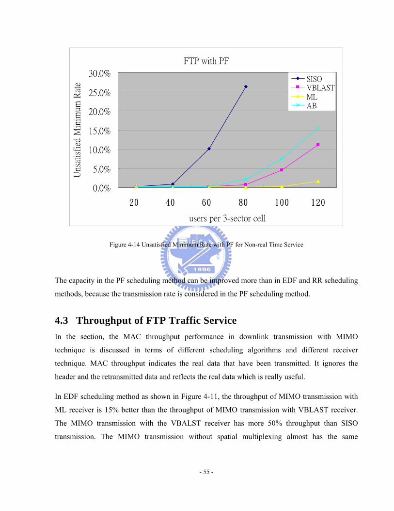
FTP with PF
00
50
100
150
200
250
300
20 40 60 80 100 120
users per 3-sector cell
Uns
atis
fied
Min
imum
Rat
eSISOVBLASTMLAB
Figure 4-14 Unsatisfied Minimum Rate with PF for Non-real Time Service
The capacity in the PF scheduling method can be improved more than in EDF and RR scheduling
methods because the transmission rate is considered in the PF scheduling method
43 Throughput of FTP Traffic Service In the section the MAC throughput performance in downlink transmission with MIMO
technique is discussed in terms of different scheduling algorithms and different receiver
technique MAC throughput indicates the real data that have been transmitted It ignores the
header and the retransmitted data and reflects the real data which is really useful
In EDF scheduling method as shown in Figure 4-11 the throughput of MIMO transmission with
ML receiver is 15 better than the throughput of MIMO transmission with VBLAST receiver
The MIMO transmission with the VBALST receiver has more 50 throughput than SISO
transmission The MIMO transmission without spatial multiplexing almost has the same
- 55 -
throughput with the MIMO transmission with VBLAST due to low VBLAST utilization as
shown in Figure 4-5
FTP with EDF
0
5
10
15
20
25
20 40 60 80 100 120
users per 3-sector cell
Thr
ough
put
(Mbp
s
Cel
l)
SISOVBLASTMLAB
Figure 4-15 Throughput with EDF
In RR scheduling method as shown in Figure 4-12 the throughput of MIMO transmission with
ML receiver is 6 better than the throughput of MIMO transmission with VBLAST receiver
The MIMO transmission with the VBALST receiver has more 40 throughput than SISO
transmission The MIMO transmission without spatial multiplexing almost has the same
throughput with the MIMO transmission with VBLAST due to low VBLAST utilization as
shown in Figure 4-5
- 56 -
FTP with RR
0
2
4
6
8
10
12
14
16
20 40 60 80 100 120
users per 3-sector cell
Thr
ough
put
(Mbp
s
Cel
l)SISOVBLASTMLAB
Figure 4-16 Throughput with RR
In MAXCINR scheduling method as shown in Figure 4-17 the throughput of MIMO
transmission with ML receiver is 55 better than the throughput of MIMO transmission with
VBLAST receiver The MIMO transmission with the VBALST receiver has more 100
throughput than SISO transmission The MIMO transmission without spatial multiplexing has
less 20 throughput than the MIMO transmission with VBLAST
- 57 -
FTP with MAXCINR
0
5
10
15
20
25
30
35
40
20 40 60 80 100 120
users per 3-sector cell
Thr
ough
put
(Mbp
s
Cel
l)
SISOVBLASTMLAB
Figure 4-17 Throughput with MAXCINR
In PF scheduling method as shown in Figure 4-18 the throughput of MIMO transmission with
ML receiver is 45 better than the throughput of MIMO transmission with VBLAST receiver
The MIMO transmission with the VBALST receiver has more 100 throughput than SISO
transmission The MIMO transmission without spatial multiplexing has less 5 throughput than
the MIMO transmission with VBLAST
- 58 -
FTP with PF
0
5
10
15
20
25
30
20 40 60 80 100 120
users per 3-sector cell
Thr
ough
put
(Mbp
s
Cel
l)
SISOVBLASTMLAB
Figure 4-18 Throughput with PF
The throughput in MAXCINR and PF scheduling methods can be improved more than in EDF
and RR scheduling methods because the transmission rate is considered in MAXCINR and PF
scheduling methods
44 Fragmentation In Figure 4-19 the channel utilization decreases when users increase in a cell since high
transmission rate may causes large padding of a burst A VOIP packet is much smaller than a
FTP packet hence the padding is more serious in VOIP traffic Exploiting padding of a burst to
adapt PDU size can reduce loss rate as shown in Figure 4-20 When users per cell increase more
loss rate can be improved There is ARQ in the simulation so PDU can be retransmitted to
reduce PER When more users stay in a cell a PDU may not be retransmitted before its delay
bound loss rate be improved obviously
- 59 -
FTP with MaxCINR
954
956
958
960
962
964
966
968
40 60 80 100 120
users per 3-sector cell
Cha
nnel
Uti
liza
tion
ML
Figure 4-19 Channel Utilization for FTP Traffic Service
VOIP with PF
00
20
40
60
80
100
120
20 40 60 80 100 120 140 160 180 200
users per 3-sector cell
Los
s Im
prov
ed R
ate
SISO
VBLASTML
AB
Figure 4-20 Improved Loss Rate in PF Scheduling Method for VOIP Traffic Service
- 60 -
Chapter 5 Conclusion and Future Work
In the thesis our contributions are the system level platform establishment of MAC layer with
MIMO technique in WiMAX standard and the performance study of MIMO transmission system
First the MAC layer with MIMO technique in IEEE 80216e system is implemented in our study
The platform is used for preliminary understanding of MIMO system Secondly utilization of
different receivers of spatial multiplexing technique in different scheduling methods is studied
Then QoS of the MIMO System with different receivers in different scheduling methods is
studied Finally the characteristic of MIMO transmission is studied and a simple fragmentation
method is applied for improving the PER
From the performance simulation we can get the conclusion as below For real time service the
VBLAST utilization of different scheduling methods is the same and the spatial multiplexing
with the ML receiver utilization of different scheduling methods is also the same Furthermore
MAXCINR and PF scheduling methods can improve more QoS than RR and EDF scheduling
methods but it is not obvious It means that there is not a scheduling method with MIMO
technique which is more appropriate than others for real time service For non-real time service
the MAXCINR scheduling method has the highest spatial multiplexing utilization and the PF
scheduling method is better than EDF and RR scheduling methods However MAXCINR is not
the most appropriate scheduling method for non-real time service because MAXCINR can not
satisfy QoS The PF scheduling method can improve more QoS and provide higher throughput
than EDF and RR scheduling methods because it considers the transmission rate Therefore the
PF is most appropriate scheduling method for non-real time service When the transmission rate
is higher the influence of the padding of a burst is more serious
The MIMO system with mixed transmit diversity and spatial multiplexing almost has the same
capacity as the MIMO system only with transmit diversity for VOIP traffic service It means that
spatial multiplexing can provide high transmission rate but is not suitable for VOIP traffic
service
In the future work we can update to the channel model the other simple radio resource
management control algorithm in the platform which is referred to power control ARQ and
- 61 -
handoff algorithm With more advance radio resource management control algorithms the
performance can be upgraded more and QoS of can be guarantee further
- 62 -
Reference
[1] IEEE ldquoIEEE Standard for Local and Metropolitan Area Networks Part 16 Air Interface
for Fixed Broadband Wireless Access Systemsrdquo IEEE Std 80216-2004 (Revision of IEEE
Std 80216-2001) pp 1-857 2004
[2] IEEE ldquoIEEE Standard for Local and metropolitan area networks Part 16 Air Interface for
Fixed and Mobile Broadband Wireless Access Systems Amendment 2 Physical and
Medium Access Control Layers for Combined Fixed and Mobile Operation in Licensed
Bands and Corrigendum 1rdquo IEEE Std 80216e-2005 and IEEE Std 80216-2004Cor
1-2005 (Amendment and Corrigendum to IEEE Std 80216-2004) pp 1-822 2006
[3] G J Foschini ldquoLayered spacendashtime architecture for wireless communication in a fading
environment when using multielement antennasrdquo Bell Labs Tech J pp 41ndash59 Autumn
1996
[4] G J Foschini and M J Gans ldquoOn limits of wireless communications in a fading
environment when using multiple antennasrdquo Wireless Pers Commun vol 6 pp
311ndash335 Mar 1998
[5] E Telatar ldquoCapacity of multiantenna Gaussian channelsrdquo ATampT Bell Laboratories Tech
Memo June 1995
[6] G Raleigh and J M Cioffi ldquoSpatial-temporal coding for wireless communicationsrdquo
IEEE Trans Commun vol 46 pp 357ndash366 1998
[7] H Boumllcskei D Gesbert and A J Paulraj ldquoOn the capacity of OFDM-based spatial
multiplexing systemsrdquo IEEE Trans Commun vol 50 pp225ndash234 Feb 2002
[8] M S Lin ldquoRadio Resource Management in Mobile WiMAX Systemrdquo a thesis submitted
to NCTU EE pp 1-81 Jun 2006
[9] F Wang A Ghosh C Sankaran and S Benes ldquoWiMAX System Performance with
Multiple Transmit and Multiple Receive Antennasrdquo in IEEE Vehicular Technology Conf
pp 2807-2811 Apr 2007
- 63 -
[10] D Gerlach and AJ Paulraj ldquoAdaptive transmitting antenna arrays with feedbackrdquo IEEE
Signal Processing Letters vol1 pp150-152 Oct 1994
[11] JH Winters ldquo Switched diversity for feedback with DPSK mobile radio systemsrdquo IEEE
Trans Veh Technol volVT-32 pp 134-150 Feb 1983
[12] RW Heath Jr S Sandhu and A J Paulraj ldquo Antenna selection for spatial multiplexing
systems with linear receiversrdquo IEEE Commun Lett vol5 pp 142-144 Apr 2001
[13] RS Blum and JW Winters ldquoOn optimum MIMO with antenna selectionrdquo IEEE Int
Conf Commun vol1 pp386-390 May 2002
[14] N Seshadri and J H Winters ldquoTwo schemes for improving the performance of
frequency-division duplex (FDD) transmission systems using transmitter antenna
diversityrdquo Int J Wireless Inform Networks vol 1 pp 49ndash60 Jan 1994
A Wittneben ldquoA new bandwidth efficient transmit antenna modulation diversity scheme
for linear digital modulationrdquo in Proc IEEE ICC vol 3 pp 1630ndash1634 1993
[15] VTarokh N Sesahdri and A R Calderbank ldquoSpace-Time codes for high data rate
wireless communication Performance criterion and code constructionrdquo IEEE Trans
Inform Theory vol44 pp744-765 Mar 1998
[16] V Tarokh H Jafarkhani and A R Calderbank ldquoSpace-Time Block codes from
orthogonal designsrdquo IEEE Trans Inform Theory vol45 pp1456-1467 Jul 1999
[17] S M Alamouti ldquoA simple transmit diversity technique for wireless communicationsrdquo
IEEE J Select Areas Commun vol16 pp 1451-1458 Oct 1998
[18] V Tarokh H Jafarkhani and A R Calderbank ldquoSpacendashtime block codes for wireless
communications Performance resultsrdquo IEEE J Select Areas Commun vol 17 pp
451ndash460 Mar 1999
[19] G Ganesan and P Stoica ldquoSpacendashtime diversity using orthogonal and amicable
orthogonal designsrdquo Wireless Pers Commun vol 18 pp 165ndash178 Aug 2001
- 64 -
[20] H Jafarkhani ldquoA quasi orthogonal space time block coderdquo IEEE Trans Commun vol
49 pp 1ndash4 Jan 2001
[21] Tirkkonen A Boariu and A Hottinen ldquoMinimal nonorthogonality rate 1 spacendashtime
block code for 3+ tx antennasrdquo in Proc IEEE Int Symp Spread Spectrum Technol pp
429ndash432 2000
[22] M O Damen A Chkeif and J C Belfiore ldquoLattice codes decoder for spacendashtime
codesrdquo IEEE Commun Lett vol 4 pp 161ndash163 May 2000
[23] P W Wolnainsky G J Foschini G D Golden and R A Valenzuela ldquoV-BLAST An
architecture for realizing very high data rates over the rich-scattering wireless channelrdquo in
Proc ISSSE pp 295-300 1998
[24] Mobile WiMAX ndash Part 1 A Technical Overview and Performance Evalutionrdquo in WiMAX
Forum pp 1-53 Jun 2006
[25] Mobile WiMAX ndash Part 2 A Comparative Analysisrdquo in WiMAX Forum pp 1-47 May
2006
[26] 3GPP ldquo3rd Generation Partnership Project Technical Specification Group Radio Access
Network Spatial channel model for Multiple Input Multiple Output (MIMO) simulations
(Release 7)rdquo 3GPP TR 25996 pp 1-40 Jun 2007
[27] M Gudmundson ldquoCorrelation Model for Shadow Fading in Mobile Radio Systemsrdquo
Elect Lett Vol 27 pp 2145-2146 Nov 1991
[28] C Wengerter J Ohohorst and AGE von Elbwart ldquoFairness and throughput analysis for
generalized proportional fair frequency scheduling in OFDMArdquo IEEE Veh Technol
Conf Vol 3 pp1903-1907 2005
[29] S Yoon Y Cho C B Chae and H Lee ldquoSystem level performance of OFDMA
forward link with proportional fair schedulingrdquo IEEE Int Symp Pers Indoor and Moblie
Radio Commun Vol 2 pp 1384-1388 Sep 2004
- 65 -
[30] S Ryu B Ryu H Seo and M Shin ldquo Urgency and Efficiency Based Packet Scheduling
Algorithm for OFDMA Wireless Systemrdquo IEEE Int Commun Conf Vol 4 pp
2779-2785 May 2005
[31] F M Chiussi and V Sivaraman ldquoAchieving high utilization in guaranteed services
networks using early-deadline-first schedulingrdquo in Proc IEEE IWQoS pp 209-217 May
1998
A Gyasi-Agyei ldquoMultiuser Diversity Based Opportunistic Scheduling for Wireless Data
Networksrdquo IEEE Commun Lett Vol 9 pp 670-672 Jul 2005
B J Chian ldquoQos-based Opportunistic Scheduling Algorithm for Mixed-traffic
Environmentrdquo A Thesis Submitted to NCTU EE pp 1-81 Jun 2007
[32] 3GPP2 ldquocdma2000 Evaluation Methodology Revision 0rdquo 3GPP2 C R 1002-0 pp1-194
Dec 2004
[33] ldquo3G amp The Future of Wirelessrdquo PDAs amp Cell Phones Vol 8 pp 48-51 May 2002
[34] ITU-T ldquoCoding of Speech at 8 kbits Using Conjugate-structure Algebraic-code-excited
Linear-predictionrdquo ITU-T Recommendation G729 pp 1-39 Mar 1996
- 66 -

throughput with the MIMO transmission with VBLAST due to low VBLAST utilization as
shown in Figure 4-5
FTP with EDF
0
5
10
15
20
25
20 40 60 80 100 120
users per 3-sector cell
Thr
ough
put
(Mbp
s
Cel
l)
SISOVBLASTMLAB
Figure 4-15 Throughput with EDF
In RR scheduling method as shown in Figure 4-12 the throughput of MIMO transmission with
ML receiver is 6 better than the throughput of MIMO transmission with VBLAST receiver
The MIMO transmission with the VBALST receiver has more 40 throughput than SISO
transmission The MIMO transmission without spatial multiplexing almost has the same
throughput with the MIMO transmission with VBLAST due to low VBLAST utilization as
shown in Figure 4-5
- 56 -
FTP with RR
0
2
4
6
8
10
12
14
16
20 40 60 80 100 120
users per 3-sector cell
Thr
ough
put
(Mbp
s
Cel
l)SISOVBLASTMLAB
Figure 4-16 Throughput with RR
In MAXCINR scheduling method as shown in Figure 4-17 the throughput of MIMO
transmission with ML receiver is 55 better than the throughput of MIMO transmission with
VBLAST receiver The MIMO transmission with the VBALST receiver has more 100
throughput than SISO transmission The MIMO transmission without spatial multiplexing has
less 20 throughput than the MIMO transmission with VBLAST
- 57 -
FTP with MAXCINR
0
5
10
15
20
25
30
35
40
20 40 60 80 100 120
users per 3-sector cell
Thr
ough
put
(Mbp
s
Cel
l)
SISOVBLASTMLAB
Figure 4-17 Throughput with MAXCINR
In PF scheduling method as shown in Figure 4-18 the throughput of MIMO transmission with
ML receiver is 45 better than the throughput of MIMO transmission with VBLAST receiver
The MIMO transmission with the VBALST receiver has more 100 throughput than SISO
transmission The MIMO transmission without spatial multiplexing has less 5 throughput than
the MIMO transmission with VBLAST
- 58 -
FTP with PF
0
5
10
15
20
25
30
20 40 60 80 100 120
users per 3-sector cell
Thr
ough
put
(Mbp
s
Cel
l)
SISOVBLASTMLAB
Figure 4-18 Throughput with PF
The throughput in MAXCINR and PF scheduling methods can be improved more than in EDF
and RR scheduling methods because the transmission rate is considered in MAXCINR and PF
scheduling methods
44 Fragmentation In Figure 4-19 the channel utilization decreases when users increase in a cell since high
transmission rate may causes large padding of a burst A VOIP packet is much smaller than a
FTP packet hence the padding is more serious in VOIP traffic Exploiting padding of a burst to
adapt PDU size can reduce loss rate as shown in Figure 4-20 When users per cell increase more
loss rate can be improved There is ARQ in the simulation so PDU can be retransmitted to
reduce PER When more users stay in a cell a PDU may not be retransmitted before its delay
bound loss rate be improved obviously
- 59 -
FTP with MaxCINR
954
956
958
960
962
964
966
968
40 60 80 100 120
users per 3-sector cell
Cha
nnel
Uti
liza
tion
ML
Figure 4-19 Channel Utilization for FTP Traffic Service
VOIP with PF
00
20
40
60
80
100
120
20 40 60 80 100 120 140 160 180 200
users per 3-sector cell
Los
s Im
prov
ed R
ate
SISO
VBLASTML
AB
Figure 4-20 Improved Loss Rate in PF Scheduling Method for VOIP Traffic Service
- 60 -
Chapter 5 Conclusion and Future Work
In the thesis our contributions are the system level platform establishment of MAC layer with
MIMO technique in WiMAX standard and the performance study of MIMO transmission system
First the MAC layer with MIMO technique in IEEE 80216e system is implemented in our study
The platform is used for preliminary understanding of MIMO system Secondly utilization of
different receivers of spatial multiplexing technique in different scheduling methods is studied
Then QoS of the MIMO System with different receivers in different scheduling methods is
studied Finally the characteristic of MIMO transmission is studied and a simple fragmentation
method is applied for improving the PER
From the performance simulation we can get the conclusion as below For real time service the
VBLAST utilization of different scheduling methods is the same and the spatial multiplexing
with the ML receiver utilization of different scheduling methods is also the same Furthermore
MAXCINR and PF scheduling methods can improve more QoS than RR and EDF scheduling
methods but it is not obvious It means that there is not a scheduling method with MIMO
technique which is more appropriate than others for real time service For non-real time service
the MAXCINR scheduling method has the highest spatial multiplexing utilization and the PF
scheduling method is better than EDF and RR scheduling methods However MAXCINR is not
the most appropriate scheduling method for non-real time service because MAXCINR can not
satisfy QoS The PF scheduling method can improve more QoS and provide higher throughput
than EDF and RR scheduling methods because it considers the transmission rate Therefore the
PF is most appropriate scheduling method for non-real time service When the transmission rate
is higher the influence of the padding of a burst is more serious
The MIMO system with mixed transmit diversity and spatial multiplexing almost has the same
capacity as the MIMO system only with transmit diversity for VOIP traffic service It means that
spatial multiplexing can provide high transmission rate but is not suitable for VOIP traffic
service
In the future work we can update to the channel model the other simple radio resource
management control algorithm in the platform which is referred to power control ARQ and
- 61 -
handoff algorithm With more advance radio resource management control algorithms the
performance can be upgraded more and QoS of can be guarantee further
- 62 -
Reference
[1] IEEE ldquoIEEE Standard for Local and Metropolitan Area Networks Part 16 Air Interface
for Fixed Broadband Wireless Access Systemsrdquo IEEE Std 80216-2004 (Revision of IEEE
Std 80216-2001) pp 1-857 2004
[2] IEEE ldquoIEEE Standard for Local and metropolitan area networks Part 16 Air Interface for
Fixed and Mobile Broadband Wireless Access Systems Amendment 2 Physical and
Medium Access Control Layers for Combined Fixed and Mobile Operation in Licensed
Bands and Corrigendum 1rdquo IEEE Std 80216e-2005 and IEEE Std 80216-2004Cor
1-2005 (Amendment and Corrigendum to IEEE Std 80216-2004) pp 1-822 2006
[3] G J Foschini ldquoLayered spacendashtime architecture for wireless communication in a fading
environment when using multielement antennasrdquo Bell Labs Tech J pp 41ndash59 Autumn
1996
[4] G J Foschini and M J Gans ldquoOn limits of wireless communications in a fading
environment when using multiple antennasrdquo Wireless Pers Commun vol 6 pp
311ndash335 Mar 1998
[5] E Telatar ldquoCapacity of multiantenna Gaussian channelsrdquo ATampT Bell Laboratories Tech
Memo June 1995
[6] G Raleigh and J M Cioffi ldquoSpatial-temporal coding for wireless communicationsrdquo
IEEE Trans Commun vol 46 pp 357ndash366 1998
[7] H Boumllcskei D Gesbert and A J Paulraj ldquoOn the capacity of OFDM-based spatial
multiplexing systemsrdquo IEEE Trans Commun vol 50 pp225ndash234 Feb 2002
[8] M S Lin ldquoRadio Resource Management in Mobile WiMAX Systemrdquo a thesis submitted
to NCTU EE pp 1-81 Jun 2006
[9] F Wang A Ghosh C Sankaran and S Benes ldquoWiMAX System Performance with
Multiple Transmit and Multiple Receive Antennasrdquo in IEEE Vehicular Technology Conf
pp 2807-2811 Apr 2007
- 63 -
[10] D Gerlach and AJ Paulraj ldquoAdaptive transmitting antenna arrays with feedbackrdquo IEEE
Signal Processing Letters vol1 pp150-152 Oct 1994
[11] JH Winters ldquo Switched diversity for feedback with DPSK mobile radio systemsrdquo IEEE
Trans Veh Technol volVT-32 pp 134-150 Feb 1983
[12] RW Heath Jr S Sandhu and A J Paulraj ldquo Antenna selection for spatial multiplexing
systems with linear receiversrdquo IEEE Commun Lett vol5 pp 142-144 Apr 2001
[13] RS Blum and JW Winters ldquoOn optimum MIMO with antenna selectionrdquo IEEE Int
Conf Commun vol1 pp386-390 May 2002
[14] N Seshadri and J H Winters ldquoTwo schemes for improving the performance of
frequency-division duplex (FDD) transmission systems using transmitter antenna
diversityrdquo Int J Wireless Inform Networks vol 1 pp 49ndash60 Jan 1994
A Wittneben ldquoA new bandwidth efficient transmit antenna modulation diversity scheme
for linear digital modulationrdquo in Proc IEEE ICC vol 3 pp 1630ndash1634 1993
[15] VTarokh N Sesahdri and A R Calderbank ldquoSpace-Time codes for high data rate
wireless communication Performance criterion and code constructionrdquo IEEE Trans
Inform Theory vol44 pp744-765 Mar 1998
[16] V Tarokh H Jafarkhani and A R Calderbank ldquoSpace-Time Block codes from
orthogonal designsrdquo IEEE Trans Inform Theory vol45 pp1456-1467 Jul 1999
[17] S M Alamouti ldquoA simple transmit diversity technique for wireless communicationsrdquo
IEEE J Select Areas Commun vol16 pp 1451-1458 Oct 1998
[18] V Tarokh H Jafarkhani and A R Calderbank ldquoSpacendashtime block codes for wireless
communications Performance resultsrdquo IEEE J Select Areas Commun vol 17 pp
451ndash460 Mar 1999
[19] G Ganesan and P Stoica ldquoSpacendashtime diversity using orthogonal and amicable
orthogonal designsrdquo Wireless Pers Commun vol 18 pp 165ndash178 Aug 2001
- 64 -
[20] H Jafarkhani ldquoA quasi orthogonal space time block coderdquo IEEE Trans Commun vol
49 pp 1ndash4 Jan 2001
[21] Tirkkonen A Boariu and A Hottinen ldquoMinimal nonorthogonality rate 1 spacendashtime
block code for 3+ tx antennasrdquo in Proc IEEE Int Symp Spread Spectrum Technol pp
429ndash432 2000
[22] M O Damen A Chkeif and J C Belfiore ldquoLattice codes decoder for spacendashtime
codesrdquo IEEE Commun Lett vol 4 pp 161ndash163 May 2000
[23] P W Wolnainsky G J Foschini G D Golden and R A Valenzuela ldquoV-BLAST An
architecture for realizing very high data rates over the rich-scattering wireless channelrdquo in
Proc ISSSE pp 295-300 1998
[24] Mobile WiMAX ndash Part 1 A Technical Overview and Performance Evalutionrdquo in WiMAX
Forum pp 1-53 Jun 2006
[25] Mobile WiMAX ndash Part 2 A Comparative Analysisrdquo in WiMAX Forum pp 1-47 May
2006
[26] 3GPP ldquo3rd Generation Partnership Project Technical Specification Group Radio Access
Network Spatial channel model for Multiple Input Multiple Output (MIMO) simulations
(Release 7)rdquo 3GPP TR 25996 pp 1-40 Jun 2007
[27] M Gudmundson ldquoCorrelation Model for Shadow Fading in Mobile Radio Systemsrdquo
Elect Lett Vol 27 pp 2145-2146 Nov 1991
[28] C Wengerter J Ohohorst and AGE von Elbwart ldquoFairness and throughput analysis for
generalized proportional fair frequency scheduling in OFDMArdquo IEEE Veh Technol
Conf Vol 3 pp1903-1907 2005
[29] S Yoon Y Cho C B Chae and H Lee ldquoSystem level performance of OFDMA
forward link with proportional fair schedulingrdquo IEEE Int Symp Pers Indoor and Moblie
Radio Commun Vol 2 pp 1384-1388 Sep 2004
- 65 -
[30] S Ryu B Ryu H Seo and M Shin ldquo Urgency and Efficiency Based Packet Scheduling
Algorithm for OFDMA Wireless Systemrdquo IEEE Int Commun Conf Vol 4 pp
2779-2785 May 2005
[31] F M Chiussi and V Sivaraman ldquoAchieving high utilization in guaranteed services
networks using early-deadline-first schedulingrdquo in Proc IEEE IWQoS pp 209-217 May
1998
A Gyasi-Agyei ldquoMultiuser Diversity Based Opportunistic Scheduling for Wireless Data
Networksrdquo IEEE Commun Lett Vol 9 pp 670-672 Jul 2005
B J Chian ldquoQos-based Opportunistic Scheduling Algorithm for Mixed-traffic
Environmentrdquo A Thesis Submitted to NCTU EE pp 1-81 Jun 2007
[32] 3GPP2 ldquocdma2000 Evaluation Methodology Revision 0rdquo 3GPP2 C R 1002-0 pp1-194
Dec 2004
[33] ldquo3G amp The Future of Wirelessrdquo PDAs amp Cell Phones Vol 8 pp 48-51 May 2002
[34] ITU-T ldquoCoding of Speech at 8 kbits Using Conjugate-structure Algebraic-code-excited
Linear-predictionrdquo ITU-T Recommendation G729 pp 1-39 Mar 1996
- 66 -
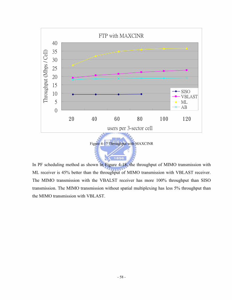
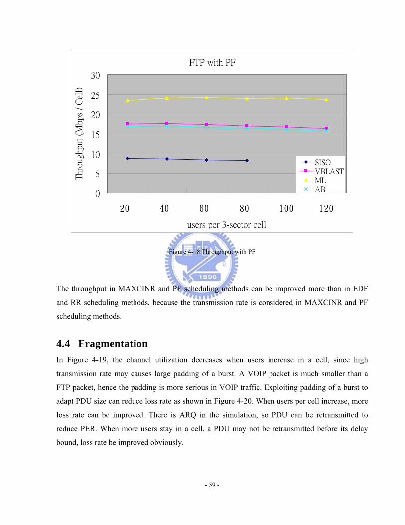