OCEAN HAZARDS ASSESSMENT - Stage 1 Report faculteit... · 2017-12-01 · Ocean Hazards Assessment -...
383
Review of Technical Requirements Numerical Modelling and Risk Assessment Marine Modelling Unit In association with: Department of Natural Resources and Mines Department of Emergency Services Environmental Protection Agency OCEAN HAZARDS ASSESSMENT - Stage 1 OCEAN HAZARDS ASSESSMENT - Stage 1 Report March 2001
Transcript of OCEAN HAZARDS ASSESSMENT - Stage 1 Report faculteit... · 2017-12-01 · Ocean Hazards Assessment -...

Review of Technical Requirements
Numerical
Modelling
and Risk
Assessment
Marine
Modelling
Unit
In association with:
Department of Natural Resources and Mines
Department of Emergency Services
Environmental Protection Agency
OCEAN
HAZARDS
ASSESSMENT
- Stage 1
OCEAN
HAZARDS
ASSESSMENT
- Stage 1
ReportMarch 2001

QQuueeeennssllaanndd CClliimmaattee
CChhaannggee
aanndd CCoommmmuunniittyy
VVuullnneerraabbiilliittyy
ttoo TTrrooppiiccaall CCyycclloonneess
OCEAN HAZARDS ASSESSMENT
- Stage 1
March 2001
SEA Doc. No. J0004-PR001C
Department of Natural Resources and Mines, Queensland Department of Emergency Services, Queensland Environmental Protection Agency, Queensland Bureau of Meteorology, Queensland Systems Engineering Australia Pty Ltd, Queensland
QNRM01056ISBN: 0 7345 1788 2
General Disclaimer
Information contained in this publication is provided as general advice only. For application to specific circumstances, advice from qualified sources should be sought.
The Department of Natural Resources and Mines, Queensland along with collaborators listed above have taken all reasonable steps and due care to ensure that the information contained in this publication is accurate at the time of production. The Department expressly excludes all liability for errors or omissions whether made negligently or otherwise for loss, damage or other consequences, which may result from this publication. Readers should also ensure that they make appropriate enquiries to determine whether new material is available on the particular subject matter.
© The State of Queensland, Department of Natural Resources and Mines 2001
Copyright protects this publication. Except for purposes permitted by the Copyright Act, reproduction by whatever means is prohibited without prior written permission of the Department of Natural Resources and Mines, Queensland.
Front cover images have been provided courtesy of the Department of Emergency Services, from the Brisbane Storm Chasers Homepage and the Queensland State Library
Enquiries should be addressed to:
Steven Crimp Department of Natural Resources and Mines 80 Meiers Road, Indooroopilly Brisbane, QLD 4068
Queensland Government Queensland Climate Change and Community Vulnerability to Tropical CyclonesOcean Hazards Assessment - Stage 1
Contents
List of Tables vii
List of Figures viii
List of Contributors xi
Acknowledgements xii
1. EXECUTIVE SUMMARY 1
2. TROPICAL CYCLONE INDUCED OCEAN HAZARDS IN QUEENSLAND 2
2.1 Overview 2
2.2 Tropical Cyclones 4
2.3 Extreme Waves 6
2.4 Storm Surge 8
2.5 Storm Tide 10
2.6 References 13
3. TROPICAL CYCLONE CLIMATOLOGY OF QUEENSLAND 14
3.1 Historical Summary of Incidence and Intensity 14
3.2 Statistical Analysis of Post 1959/60 Data 16
3.3 Climatic Variability 23
3.4 Conclusions and Recommendations 27
3.5 References 27
4. GREENHOUSE CLIMATE CHANGE AND SEA LEVEL RISE 29
4.1 The Global Warming Process 29
4.2 Evidence of Climate Change 30
4.3 Latest Global Projections 32
4.4 Major Weather Systems and Global Climate Change 33
4.5 Impact on the Oceans 34
4.6 Impact on Coastal Zones and Small Islands 35
4.7 Australian Regional Predictions and Impacts 37
J0004-PR0001C i March 2001
Queensland Government Queensland Climate Change and Community Vulnerability to Tropical CyclonesOcean Hazards Assessment - Stage 1
4.8 Conclusions and Recommendations 37
4.9 References 38
5. TROPICAL CYCLONE WIND AND PRESSURE MODELLING 41
5.1 The Need for Simplified Models 41
5.2 Basic Model Characteristics 42
5.3 Boundary Layer Representation 44
5.4 Forward Motion Asymmetry 45
5.5 A Typical Parametric Wind Field Representation 46
5.6 Historical Development of Windfield Models 48
5.6.1 Earliest Studies 485.6.2 US Army Corps of Engineers Impetus 485.6.3 Growth of Applications 495.6.4 Improving Theory and Observations 515.6.5 More Contemporary Developments 525.6.6 Transient Wind Features 555.6.7 Summary of Model Developments 56
5.7 Conclusions and Recommendations 57
5.8 References 58
6. NUMERICAL MODELLING OF TROPICAL CYCLONE STORM SURGE 67
6.1 Background and Introduction 67
6.2 Essential Physics – The Long Wave Equations 68
6.2.1 Equations of Motion 686.2.2 Boundary Conditions 706.2.3 Surge-tide Interactions 72
6.3 External Forcing 72
6.3.1 Wind field modelling 726.3.2 Parameterisation of surface stress 73
6.4 Solution Procedures 76
6.4.1 Finite Difference versus Finite Element 766.4.2 Explicit vs Implicit 776.4.3 Sizes for spatial step and time step 786.4.4 Open Boundary Conditions 796.4.5 Overland Flooding and Drying 82
6.5 Recent Developments 85
6.5.1 Surge-Wave Interactions 85
6.6 Conclusions and Recommendations 88
6.7 References 91
J0004-PR0001C ii March 2001

Queensland Government Queensland Climate Change and Community Vulnerability to Tropical CyclonesOcean Hazards Assessment - Stage 1
7. NUMERICAL MODELLING OF TROPICAL CYCLONE WIND WAVES 99
7.1 Introduction 99
7.2 The Physics of Wind-Wave Evolution 99
7.2.1 Governing Equations 997.2.2 Source Terms 100
7.3 Numerical Modelling of Waves 101
7.3.1 Introduction 1017.3.2 Source Term Representation 1027.3.3 First Generation Models 1027.3.4 Second Generation Models 1047.3.5 Third Generation Models 105
7.4 Computational Aspects 106
7.4.1 Advection of Energy 1077.4.2 Computational Grids 1107.4.3 Initial and Boundary Conditions 111
7.5 The Tropical Cyclone Wave Field 111
7.6 Tropical Cyclone Wave Spectra 116
7.6.1 JONSWAP Representation of Tropical Cyclone Spectra 1187.6.2 Donelan et al. (1985) representation of Tropical Cyclone Spectra 121
7.7 Conclusions and Recommendations 123
7.7.1 Choice of Model Physics 1237.7.2 Grid Considerations 1247.7.3 Dissipation on Reefs 125
7.8 References 125
8. ESTIMATION OF WAVE SETUP AND RUNUP 131
8.1 Introduction 131
8.2 Waves in the Surf Zone 131
8.2.1 The Surf Similarity Parameter 1328.2.2 Breaker Types 1328.2.3 Breaker Heights 1338.2.4 Wave Height to Water Depth Ratio after Breaking 1338.2.5 Surf Beat 134
8.3 The Shape of the Surf Zone Mean Water Surface 134
8.3.1 Terminology and Definitions 1348.3.2 Wave Setdown 1368.3.3 Wave Setup 1368.3.4 Shoreline Setup 1388.3.5 Wave Effects on River Tail-water Levels 139
8.4 Swash and Runup Heights 141
8.4.1 Introduction 1418.4.2 Runup heights for Regular Waves 1418.4.3 Runup Heights for Irregular Waves 1428.4.4 Extreme Runup Levels 143
8.5 Wave Setup on Coral Reefs 144
J0004-PR0001C iii March 2001

Queensland Government Queensland Climate Change and Community Vulnerability to Tropical CyclonesOcean Hazards Assessment - Stage 1
8.6 Conclusions and Recommendations 148
8.7 References 149
9. STORM TIDE STATISTICS 150
9.1 Introduction 150
9.2 The Historical Context 150
9.3 The Need for Revision and Update 153
9.4 The Prediction Problem 155
9.5 Estimation of Risks Without Long-Term Measured Data 156
9.5.1 The "Design Storm" Approach 1569.5.2 The "Hindcast" Approach 1569.5.3 Simulation Techniques 157
9.6 Essential Elements for Statistical Storm Tide Prediction 160
9.6.1 Representation of the Storm Climatology 1609.6.2 Representation of the Deterministic Forcing and Ocean Response 1619.6.3 Representation of the Combined Storm Tide Event 162
9.7 Conclusions and Recommendations 163
9.8 References 164
10. STORM SURGE MODEL VALIDATION AND SENSITIVITY TESTING 169
10.1 Selection of Hindcast Storms 169
10.2 Details of the Numerical Storm Surge Modelling 169
10.3 The January 1918 Cyclone at Mackay 177
10.3.1 Available Tropical Cyclone Data 17710.3.2 Available Storm Tide Data 17810.3.3 Reconstruction of the Event 18210.3.4 Model and Data Comparisons 18810.3.5 Implications for Storm Surge Modelling 19110.3.6 Tidal Modelling 19210.3.7 Storm Surge Modelling 19310.3.8 References 197
10.4 Tropical Cyclone Althea December 1971 at Townsville 198
10.4.1 Available Data 19810.4.2 Reconstruction of the Event 20310.4.3 Implications for Storm Surge Modelling 21410.4.4 Tidal Modelling 21510.4.5 Storm Surge Modelling 21510.4.6 References 224
10.5 Tropical Cyclone Ted December 1976 at Burketown 225
10.5.1 Available Data 22510.5.2 Reconstruction of the Event 22810.5.3 Implications for Storm Surge Modelling 23510.5.4 Tidal Modelling 23610.5.5 Storm Surge Modelling 236
J0004-PR0001C iv March 2001
Queensland Government Queensland Climate Change and Community Vulnerability to Tropical CyclonesOcean Hazards Assessment - Stage 1
10.5.6 References 243
10.6 Tropical Cyclone Steve February 2000 at Cairns 244
10.6.1 Available Data 24410.6.2 Reconstruction of the Event 24810.6.3 Implications for Storm Surge Modelling 25710.6.4 Tidal Modelling 25810.6.5 Storm Surge Modelling 25810.6.6 References 264
10.7 Summary and Conclusions 265
11. SYSTEM DESIGN CONSIDERATIONS FOR STORM TIDE PREDICTION 268
11.1 Storm Tide Warning - the MEOW Approach 269
11.1.1 The Envisaged BMRC Procedure 26911.1.2 Conclusions 271
11.2 Storm Tide Planning - Statistical Approaches 271
11.3 A Suggested Hybrid Approach 273
11.4 Storm Surge Model Domains for the Queensland Coast 276
11.4.1 Selection Rationale 27711.4.2 Model Domain Specification 277
11.5 Estimating Model Simulation Times and Storage Requirements 279
11.5.1 Model Requirements 28011.5.2 MEOW Parameter Selection 282
11.6 Conclusions and Recommendations 286
11.7 References 287
12. OPERATIONAL CONSIDERATIONS FOR A STORM TIDE FORECAST SYSTEM 289
12.1 Background 289
12.1.1 NMOC Operational Storm Tide Model Interface 28912.1.2 Queensland Regional Office MEOW Display System 29012.1.3 Planned AIFS Tropical Cyclone Module 29012.1.4 Existing Sanderson et al. (1995) Methodology 291
12.2 Functional Specification 291
12.2.1 Background 29112.2.2 Scope 29112.2.3 Accuracy 29212.2.4 Functionality 29212.2.5 Input Requirements 29312.2.6 Computational Requirements 29412.2.7 Output Requirements 29612.2.8 Forecast Products 29712.2.9 Use Cases 29712.2.10 Associated Tools 297
12.3 Conclusions and Recommendations 298
12.4 References 299
J0004-PR0001C v March 2001
Queensland Government Queensland Climate Change and Community Vulnerability to Tropical CyclonesOcean Hazards Assessment - Stage 1
13. DISSEMINATION OF TROPICAL CYCLONE STORM TIDE HAZARDINFORMATION 300
13.1 General 300
13.2 Principal Stakeholder Groups 301
13.2.1 Government/Political 30113.2.2 Industry/Commerce 30213.2.3 Professional 30313.2.4 Education and Media 303
13.3 The Key Stakeholders and/or Key Methods of Information Delivery 303
13.3.1 Bureau of Meteorology 30313.3.2 Emergency Management Australia (EMA) 30513.3.3 Queensland Department of Communication, Information, Local Govt, Planning and Sport 30513.3.4 Queensland Department of Emergency Services (DES) 30513.3.5 Queensland Environmental Protection Agency (EPA) 30613.3.6 Queensland Local Government Authorities 30713.3.7 Industry Associations 30813.3.8 Professional Bodies 308
13.4 Potential Information Products 309
13.4.1 Media Delivery Mechanisms 30913.4.2 Content 30913.4.3 Associated Knowledge Needs 310
13.5 Conclusions and Recommendations 310
13.6 References 311
14. SUMMARY CONCLUSIONS AND RECOMMENDATIONS 313
APPENDICES 317
A Extract from the Scope of Work
B Summary Parameters of all Tropical Cyclones in Queensland since 1906/07
C Tropical Cyclone Wind and Pressure Model
D Technical Description of the James Cook University Storm Surge Model (MMUSURGE)
E Present US Practice for MEOW Storm Tide Warnings
F Details of Supplied MEOW Model A and B Domains
G Recommended MEOW Technique for Storm Tide Forecasting
H MEOW Database Requirements and Storage Costs
J0004-PR0001C vi March 2001

Queensland Government Queensland Climate Change and Community Vulnerability to Tropical CyclonesOcean Hazards Assessment - Stage 1
List of Tables
Table 2.1 Australian tropical cyclone category scale. 5Table 2.2 Summary of significant Queensland storm tides. 12Table 3.1 Data base quality assessment for the Eastern Region (after Holland 1981) 16Table 3.2 Summary ENSO statistics for Queensland. 24Table 4.1 IS92a projected sea level increases to 2100 32Table 5.1 Example Storm Parameter Set 46Table 6.1 Various formulations for surface drag coefficient C10 75Table 6.2 Example calculations of space and time steps 79Table 7.1 The relative importance of various physical mechanisms in different domains. 101Table 7.2 Definition of model classes based on the representation of the source terms. 102Table 8.1 Surf similarity parameter ranges. 132Table 9.1 Previous storm tide statistics studies in Queensland. 152Table 9.2 Summary of the simulation methods. 163Table 10.1 Hindcast storm set. 169Table 10.2 Hindcast model domains. 170Table 10.3 Tidal boundary information. 170Table 10.4 Model sensitivity tests undertaken. 171Table 10.5 Adopted hindcast parameters for the January 1918 cyclone. 186Table 10.6 Observer locations during Mackay 1918. 188Table 10.7 Summary of estimated peak storm surge amplitude for Althea. 202Table 10.8 Indicative radius to maximum winds for Althea. 205Table 10.9 Adopted hindcast parameters for tropical cyclone Althea. 206Table 10.10 Adopted hindcast parameters for tropical cyclone Ted. 229Table 10.11 Summary of measured storm surge magnitudes for Steve. 247Table 10.12 Adopted radius to maximum winds for Steve. 248Table 10.13 Adopted hindcast parameters for tropical cyclone Steve. 249Table 10.14 Summary of storm surge model hindcast accuracy. 266Table 11.1 Scale considerations in model domain selection. 277Table 11.2 Selected MEOW model domain parameters. 278Table 11.3 CPU and disk storage requirements for MMUSURGE on the CIRRUS1 workstation. 281Table 11.4 Estimated run times and storage needs for example MEOW scenarios. 283Table 11.5 Benefit of multiple CPUs for MEOW Scenario 2. 285
J0004-PR0001C vii March 2001

Queensland Government Queensland Climate Change and Community Vulnerability to Tropical CyclonesOcean Hazards Assessment - Stage 1
List of Figures
Figure 2.1 The tropical cyclone storm tide hazard assessment process. 3Figure 2.2 Tropical cyclone Fran approaching the Queensland coast in March 1992. 4Figure 2.3 Water level components of a storm tide. 9Figure 2.4 Effect of tide, storm surge and wave setup phasing on storm tide level. 10Figure 3.1 Historical trends for tropical cyclones in the Queensland region 15Figure 3.2 The post-1959/60 tropical cyclone dataset for Queensland. 17Figure 3.3 Tropical cyclone seasonal occurrence and duration post 1959/60. 18Figure 3.4 Tropical cyclone forward speed and direction post-1959. 19Figure 3.5 Seasonal track variation of tropical cyclones post-1959. 20Figure 3.6 Smoothed statistical analyses of post-1959 tropical cyclone track data 22Figure 3.7 Decadal tropical cyclone track variability post-1959. 25Figure 3.8 ENSO variation in tropical cyclone tracks post-1959. 26Figure 4.1 The Earth's radiation and energy balance in W m-2 30Figure 4.2 Combined trends in land-surface air and sea-surface temperature anomalies 31Figure 4.3 Australian long-term sea level records (after PCTMSL 1999) 31Figure 4.4 1990 to 2100 sea level rise for scenario IS92a (after IPCC 1996b, fig 9-3) 33Figure 5.1 Basic radial wind and pressure profiles in a tropical cyclone. 42Figure 5.2 Example surface mean wind field for a moving storm. 47Figure 5.3 Some example parametric radial wind profiles. 57Figure 6.1 Schematic layout of model geometry in Cartesian coordinates (x,y,z). 70Figure 6.2 C10 as a function of U10 for formulations 1, 4 and 5 of Table 6.1. 75Figure 7.1 A diagrammatic representation of wind wave generation and propagation in the coastal region, with a
number of the important physical processes shown [Holthuijsen pers. comm.]. 99Figure 7.2 The source term balance for first generation wave models. 103Figure 7.3 The source term balance for second generation wave models. 105Figure 7.4 The source term balance for third generation wave models. 107Figure 7.5 The directional wave spectrum. 108Figure 7.6 The natural dispersion of the bin of energy as it is advected. 109Figure 7.7 Schematic diagram showing the generation of waves within a translating hurricane (i.e northern
hemisphere view). 113Figure 7.8 The wave height distribution as predicted by the numerical model results of Young (1988b). 115Figure 7.9 Contours of the equivalent fetch within a tropical cyclone. As proposed by Young and Burchell
(1996). 116Figure 7.10 Values of the exponent in the relationship plotted as a function of the inverse wave age for the
tropical cyclone data of Young (1997). 119Figure 7.11 JONSWAP spectral parameters for tropical cyclone conditions. 120Figure 7.12 Donelan et al. (1985) spectral parameters for tropical cyclone conditions. 122Figure 8.1 The wave breaking phenomenon. 132Figure 8.2 A surf zone bore carrying large amounts of suspended sand. 133Figure 8.3 An example of surf beat. 134Figure 8.4 Definitions of surf zone levels and depths. 135Figure 8.5 Time averaged, horizontal forces due to wind, waves and gravity acting on a surf zone control
volume. 135Figure 8.6 Setup profile in a natural surf zone. 138Figure 8.7 Observed shoreline setup on a wide variety of beaches. 139Figure 8.8 Scour hole on the beach side of the southern Brunswick breakwater. 140Figure 8.9 Tidal anomaly (measured tide minus predicted tide). 140Figure 8.10 Bore collapsing at the beach face where it encounters zero depth and generating swash. 141Figure 8.11 Relationship between the vertical scale LR in the Rayleigh runup distribution and the offshore wave
parameters. 142Figure 8.12 Coral reef wave setup definitions (after Gourlay 1997). 144
Figure 8.13 Kp and Kp' as a function of tan (after Gourlay 1997). 147Figure 9.1 Some existing storm tide statistics for selected Queensland locations 153Figure 10.1 Overview of Coral Sea hindcast grids. 172
J0004-PR0001C viii March 2001

Queensland Government Queensland Climate Change and Community Vulnerability to Tropical CyclonesOcean Hazards Assessment - Stage 1
Figure 10.2 Mackay hindcast grid. 173Figure 10.3 Townsville hindcast grids. 174Figure 10.4 Cairns hindcast grids. 175Figure 10.5 Gulf of Carpentaria hindcast grids. 176Figure 10.6 Extent of inundation due to the storm tide during Mackay 1918 179Figure 10.7 Established storm tide information for Mackay 1918. 180Figure 10.8 Mackay 1918 synoptic development (after Bath 1957). 182Figure 10.9 Mackay 1918 storm track (after Bath 1957). 183Figure 10.10 Collective pressure observations during Mackay 1918. 184Figure 10.11 Reconstructed cyclone track and wind and pressure fields at landfall for Mackay 1918. 187Figure 10.12 Comparison of modelled and measured pressures for Mackay 1918. 189Figure 10.13 Comparison of wind speeds and directions for Mackay 1918. 190Figure 10.14 Modelled envelope of maximum winds and minimum pressure for Mackay 1918. 191Figure 10.15 Comparison of modelled and predicted tide during Mackay 1918. 192Figure 10.16 Water levels prior to storm landfall (no tide case) for Mackay 1918. 193Figure 10.17 Storm tide elevations and velocities at landfall (tide included) for Mackay 1918. 194Figure 10.18 Time history comparisons of modelled and measured water levels for the Mackay 1918 cyclone.
195Figure 10.19 Influence of the Great Barrier Reef on Mackay 1918. 196Figure 10.20 Synoptic situation for Althea (after Callaghan 2000) 199Figure 10.21 Radar images of Althea (after Callaghan 1996). 200Figure 10.22 Barograph (top) and anemograph (bottom) from Townsville Airport. 201Figure 10.23 Alongshore variation in estimated peak storm surge amplitude for Althea. 203Figure 10.24 Tidal record at Townsville harbour during Althea. 204Figure 10.25 Tidal record at Bowen harbour during Althea. 204Figure 10.26 Reconstructed cyclone track and wind and pressure fields near landfall for Althea. 207Figure 10.27 Modelled and measured pressures and winds at Lihou Reef for Althea. 208Figure 10.28 Modelled and measured pressures and winds at Willis Island for Althea. 209Figure 10.29 Modelled and measured pressures and winds at Flinders Reef for Althea. 210Figure 10.30 Location of the Townsville AMO instrumentation. 211Figure 10.31 Modelled and measured pressures and winds at Townsville AMO for Althea. 212Figure 10.32 Modelled and measured pressures and winds at Cardwell for Althea. 213Figure 10.33 Modelled envelope of maximum winds and minimum pressure for Althea. 214Figure 10.34 Comparison of modelled and predicted tide at Townsville Harbour. 215Figure 10.35 Effect of windfield asymmetry on surge response. 216Figure 10.36 Modelled surge-only response of Althea 6 h before landfall. 217Figure 10.37 Nearshore surge-only response of Althea near time of landfall. 218Figure 10.38 Measured and modelled storm tide at Townsville Harbour. 219Figure 10.39 2D versus 3D model prediction for Althea. 220Figure 10.40 Measured and modelled storm tide levels at Bowen for Althea. 220Figure 10.41 Measured and modelled surge component at Townsville Harbour for Althea. 221Figure 10.42 Influence of grid resolution on accuracy for Althea. 222Figure 10.43 Influence of time step on accuracy for Althea. 222Figure 10.44 Comparison of modelled and measured alongshore surge profile for Althea. 223Figure 10.45 Satellite image of Ted (BoM photo) 226Figure 10.46 Ted synoptic situation (after Callaghan 2000). 226Figure 10.47 Tidal record from CSIRO observers at Karumba during Ted. 227Figure 10.48 Reconstructed cyclone track and wind and pressure fields at landfall for Ted. 230Figure 10.49 Modelled and measured pressures and winds at Burketown for Ted. 231Figure 10.50 Modelled and measured pressures and winds at Mornington Island for Ted. 232Figure 10.51 Modelled and measured pressures and winds at Augustus Downs for Ted. 233Figure 10.52 Modelled pressures and winds at Karumba for Ted. 234Figure 10.53 Modelled envelope of maximum winds and minimum pressure for Ted. 235Figure 10.54 Modelled and measured tides at Karumba for Ted. 237Figure 10.55 Measured and modelled tides at Mornington Island for Ted. 237Figure 10.56 Storm surge response of Ted without tide. 238Figure 10.57 Measured and modelled surge height at Karumba for Ted. 239Figure 10.58 Measured and modelled surge height at Mornington Island for Ted. 239Figure 10.59 Measured and modelled absolute water levels at Karumba for Ted. 241Figure 10.60 Measured and modelled absolute water levels at Mornington Island Ted. 241
J0004-PR0001C ix March 2001
Queensland Government Queensland Climate Change and Community Vulnerability to Tropical CyclonesOcean Hazards Assessment - Stage 1
Figure 10.61 Example of overland flooding peaks for Ted increasing after peak storm tide. 242Figure 10.62 Synoptic situation for Steve (after Callaghan 2000) 245Figure 10.63 GMS 5 satellite image of Steve a few hours before landfall. 245Figure 10.64 Radar image of Steve near landfall. 246Figure 10.65 Anemograph from Cairns Airport during Steve. 246Figure 10.66 Tidal record at Cairns harbour during Steve. 247Figure 10.67 Reconstructed Steve track and wind and pressure fields near landfall. 250Figure 10.68 Modelled and measured pressures and winds at Flinders Reef for Steve. 251Figure 10.69 Modelled and measured pressures and winds at Holmes Reef for Steve. 252Figure 10.70 Modelled and measured pressures and winds at Bougainville Reef for Steve. 253Figure 10.71 Modelled and measured pressures and winds at Green Island for Steve. 254Figure 10.72 Modelled and measured pressures and winds at Cairns Airport for Steve. 255Figure 10.73 Location of the Cairns Airport instrumentation. 256Figure 10.74 Modelled envelope of Steve maximum winds and minimum pressure. 257Figure 10.75 Modelled and predicted tides at Cairns Harbour for Steve. 258Figure 10.76 Steve modelled storm surge levels 8 h before landfall. 259Figure 10.77 Steve modelled storm surge circulation 8 h before landfall. 260Figure 10.78 Modelled and measured storm surge at Cairns Harbour for Steve. 261Figure 10.79 Storm surge levels in Trinity Inlet near the time of cyclone Steve landfall. 262Figure 10.80 Storm surge velocity in Trinity Inlet near the time of cyclone Steve landfall. 263Figure 10.81 Measured and modelled total water level at Cairns Harbour during Steve. 264Figure 11.1 The MEOW warning technique. 269Figure 11.2 The MEOW storm surge generation step. 270Figure 11.3 Recommended options for statistical storm tide estimation. 272Figure 11.4 MIRAM parametric storm tide model prediction for Althea. 274Figure 11.5 MIRAM parametric model prediction for the 1918 Mackay. 274Figure 11.6 A suggested hybrid approach to the storm tide prediction problem. 276Figure 11.7 Storm surge model A and B domains for the Queensland coast. 279Figure 11.8 Summary MEOW resource requirements for 24 h "Option (iii)". 284Figure 12.1 Schematic operation of a MEOW forecast tool. 292Figure 13.1 The potentially broad range of stakeholders of tropical cyclone storm tide hazard information. 300Figure 13.2 Suggested matchings between potential information products and various community sectors. 312
J0004-PR0001C x March 2001

Queensland Government Queensland Climate Change and Community Vulnerability to Tropical CyclonesOcean Hazards Assessment - Stage 1
List of Contributors
Systems Engineering Australia Pty Ltd Bruce Harper BE PhD FIEAust CPEng RPEQ 7 Mercury Ct Bridgeman Downs Qld 4035 DirectorACN 073 544 439 Editor
Principal author all Chapters except 6, 7 and
8.2 to 8.4.
James Cook University Thomas Hardy BS MS PhD Department of Civil and Environmental Assoc. Prof. and Principal Academic Adviser Engineering Director, Marine Modelling Unit
Chapters 6, part 9 and 11.
Luciano Mason BE MIEAust Research Engineer, Marine Modelling Unit Chapters 6, part 10 and 11, Appendix D and F.
James Cook University Lance Bode BSc PhD Department of Mathematics and Statistics Senior Lecturer
Oceanographer, Marine Modelling Unit Chapter 6, Appendix D.
Adelaide University Ian Young BE MEngSc PhD FIEAust Faculty of Engineering, Computer Professor and Executive Dean and Mathematical Sciences Chapter 7.
The University of Queensland Peter Nielsen ME PhD DE Department of Civil Engineering Associate Professor
Chapter 8 sections 8.2 to 8.4.
J0004-PR0001C xi March 2001
Queensland Government Queensland Climate Change and Community Vulnerability to Tropical CyclonesOcean Hazards Assessment - Stage 1
Acknowledgements
This project was funded through a Greenhouse Special Treasury Initiative managed by the Queensland Department of Natural Resources and Mines. Project management was provided by the Bureau of Meteorology Queensland Regional Office (JimDavidson, Supervising Meteorologist) assisted by a Project Management Committee withrepresentatives from the Department of Natural Resources and Mines (Steven Crimp), the Department of Emergency Services (Lesley Galloway) and the Environmental Protection Agency (David Robinson and Michael Allen).
The cooperation of Bureau of Meteorology staff in the Queensland Regional Office is gratefully acknowledged, especially Jim Davidson, Jeff Callaghan, Michael Berechree, SueOates and Matt Saunderson. Jeff Kepert (Bureau of Meteorology Research Centre) provided comment on the identified issue of asymmetry of tropical cyclone windfields. In addition, John Broadbent (Queensland Transport) greatly assisted through the supply of recorded water level data. Michael Gourlay and Jennifer Hacker (University of Queensland) assisted through provision of historical information regarding the Mackay 1918 storm. Ken Granger (AGSO)provided information on ground elevations in the Mackay area as well as a diagram of the flooded area during the Mackay 1918 event. Peter Croker (Caloundra) assisted in the locating of the family home "Bona Vista" in Mackay during 1918 and provided extracts from a letter written by his mother who described the cyclone effects at the Eimeo Hotel. David Robinson (EPA) provided Department of Harbours and Marine archive material in regard to tropical cyclone Ted in 1976. Jason McConochie (James Cook University) assisted in developing the numerical model documentation and Wesley Bailey assisted in model domain generation.
The Project Management Committee particularly wishes to acknowledge the significant contribution by Rex Falls, former Regional Director of the Bureau of Meteorology, Queensland, whose efforts led to the establishment of the project.
B. Harper T. Hardy
J0004-PR0001C xii March 2001

Queensland Government Queensland Climate Change and Community Vulnerability to Tropical CyclonesOcean Hazards Assessment - Stage 1
1. Executive Summary
The Bureau of Meteorology, in conjunction with a number of Queensland Governmentagencies and with financial support from the Greenhouse Special Treasury Initiative,commissioned the present study to assess the magnitude of the ocean threat from tropical cyclones in Queensland. The overall project is intended to update and extend the presentunderstanding of the threat of storm tide inundation in Queensland on a state-wide scale including the effects of storm wave conditions in selected areas, and estimates of potential Greenhouse impacts.
The overall project scope is outlined in Appendix A, while the present report addresses only Stage 1 of the project, which is limited to:
a) A review of technical requirements in order to further develop the project;
Reviewing current knowledge and making technical recommendations for the overall project.
Appraising and adapting the James Cook University (JCU) storm surge model(MMUSURGE) software for the purposes of the project.
b) State-wide numerical simulations of tropical cyclone storm surge;
Installing the MMUSURGE storm surge modelling software on the Bureau's computersystem in Brisbane.
Assisting the Bureau in undertaking storm surge modelling for the Queensland coast.
The specific work items under Stage 1 were:
Part A: Review of Project Technical Requirements.A-1 Assessment of Greenhouse climate change and sea level rise. A-2 Review the technical requirements for numerical modelling of cyclone storm surge. A-3 Review the technical requirements for numerical modelling of cyclone wind waves. A-4 Database design. A-5 Review the technical requirements for an operational MEOWs system.A-6 Dissemination of results.
Part B: Numerical Modelling of Tropical Cyclone Storm Surge.B-1 Establishment of the storm surge modelling system and database. B-2 Production of numerical simulation data.
The above scope items have been addressed within a developmental context which aims to provide a complete overview of the technical needs for assessment of ocean hazards for tropical cyclones in Queensland, taking account of climate change and community vulnerability issues. Each report chapter provides its own specific recommendations, which are brought together in Chapter 14 as a series of major recommendations, re-framed toaddress the original workscope items as listed above.
It is concluded that much of the work requiring to be done under subsequent stages of theproject can be achieved with existing tools and methodologies. There are some items however which will greatly benefit from modest but immediate research and development efforts.
J0004-PR0001C 1 March 2001
Queensland Government Queensland Climate Change and Community Vulnerability to Tropical CyclonesOcean Hazards Assessment - Stage 1
2. Tropical Cyclone Induced Ocean Hazards in Queensland
This study is concerned with the risk assessment of ocean hazards associated with tropical cyclones throughout Queensland. This chapter provides a brief contextual overview of the problem and introduces the various hazard elements, which are addressed more completely insubsequent chapters.
2.1 Overview
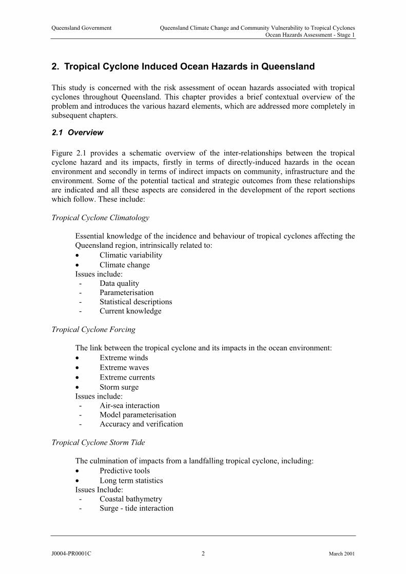
Figure 2.1 provides a schematic overview of the inter-relationships between the tropical cyclone hazard and its impacts, firstly in terms of directly-induced hazards in the ocean environment and secondly in terms of indirect impacts on community, infrastructure and the environment. Some of the potential tactical and strategic outcomes from these relationships are indicated and all these aspects are considered in the development of the report sectionswhich follow. These include:
Tropical Cyclone Climatology
Essential knowledge of the incidence and behaviour of tropical cyclones affecting theQueensland region, intrinsically related to:
Climatic variability
Climate change Issues include:- Data quality- Parameterisation- Statistical descriptions- Current knowledge
Tropical Cyclone Forcing
The link between the tropical cyclone and its impacts in the ocean environment:
Extreme winds
Extreme waves
Extreme currents
Storm surge Issues include:- Air-sea interaction- Model parameterisation- Accuracy and verification
Tropical Cyclone Storm Tide
The culmination of impacts from a landfalling tropical cyclone, including:
Predictive tools
Long term statistics Issues Include:- Coastal bathymetry- Surge - tide interaction
J0004-PR0001C 2 March 2001

Queensland Government Queensland Climate Change and Community Vulnerability to Tropical CyclonesOcean Hazards Assessment - Stage 1
- Localised wave effects - Inundation - Statistical representation
Vulnerability
The various elements at risk from the tropical cyclone hazard:
Community
Infrastructure
EnvironmentIssues include:- Predictive tools- Communication - Logistics and organisation - Planning and legislation
Climatic
Variability
Climate
Change
Tropical
Cyclone
Climatology
Tropical Cyclone Forcing
Wind Waves Current Surge
Storm Tide Tide
Vulnerability
Tactical
Responses
Strategic
Responses
Warnings
Evacuations
Planning
Legislation
Community EnvironmentInfrastructure
Figure 2.1 The tropical cyclone storm tide hazard assessment process.
J0004-PR0001C 3 March 2001
Queensland Government Queensland Climate Change and Community Vulnerability to Tropical CyclonesOcean Hazards Assessment - Stage 1
2.2 Tropical Cyclones
Tropical cyclones are large scale and potentially very severe low pressure weather systemsthat affect the Queensland region typically between November and April, with an averageincidence of 5.2 storms per year since 1959/60 (refer Chapter 3).
The strict definition of a tropical cyclone (WMO, 1997) is:
A non-frontal cyclone of synoptic scale developing over tropical waters and having a definite organized wind circulation with average wind of 34 knots (63 km h
-1) or more
surrounding the centre.
The tropical cyclone is an intense tropical low pressure weather system where, in the southernhemisphere, winds circulate clockwise around the centre. In Australia, such systems are upgraded to severe tropical cyclone status (referred to as hurricanes or typhoons in somecountries) when average, or sustained, surface wind speeds exceed 120 kmh-1. Theaccompanying shorter-period destructive wind gusts are often 50 per cent or more higher than the sustained winds.
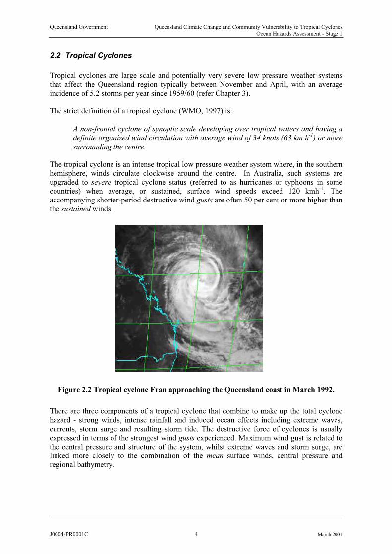
Figure 2.2 Tropical cyclone Fran approaching the Queensland coast in March 1992.
There are three components of a tropical cyclone that combine to make up the total cyclonehazard - strong winds, intense rainfall and induced ocean effects including extreme waves,currents, storm surge and resulting storm tide. The destructive force of cyclones is usually expressed in terms of the strongest wind gusts experienced. Maximum wind gust is related tothe central pressure and structure of the system, whilst extreme waves and storm surge, arelinked more closely to the combination of the mean surface winds, central pressure andregional bathymetry.
J0004-PR0001C 4 March 2001
Queensland Government Queensland Climate Change and Community Vulnerability to Tropical CyclonesOcean Hazards Assessment - Stage 1
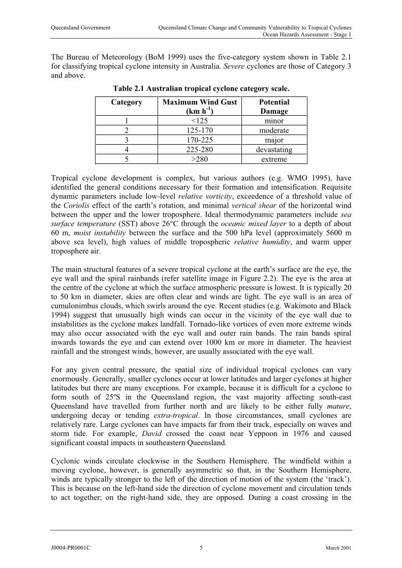
The Bureau of Meteorology (BoM 1999) uses the five-category system shown in Table 2.1 for classifying tropical cyclone intensity in Australia. Severe cyclones are those of Category 3 and above.
Table 2.1 Australian tropical cyclone category scale.
Category Maximum Wind Gust
(km h-1
)
Potential
Damage
1 <125 minor
2 125-170 moderate
3 170-225 major
4 225-280 devastating
5 >280 extreme
Tropical cyclone development is complex, but various authors (e.g. WMO 1995), have identified the general conditions necessary for their formation and intensification. Requisitedynamic parameters include low-level relative vorticity, exceedence of a threshold value ofthe Coriolis effect of the earth’s rotation, and minimal vertical shear of the horizontal wind between the upper and the lower troposphere. Ideal thermodynamic parameters include sea
surface temperature (SST) above 26°C through the oceanic mixed layer to a depth of about 60 m, moist instability between the surface and the 500 hPa level (approximately 5600 m above sea level), high values of middle tropospheric relative humidity, and warm uppertroposphere air.
The main structural features of a severe tropical cyclone at the earth’s surface are the eye, theeye wall and the spiral rainbands (refer satellite image in Figure 2.2). The eye is the area at the centre of the cyclone at which the surface atmospheric pressure is lowest. It is typically 20to 50 km in diameter, skies are often clear and winds are light. The eye wall is an area ofcumulonimbus clouds, which swirls around the eye. Recent studies (e.g. Wakimoto and Black 1994) suggest that unusually high winds can occur in the vicinity of the eye wall due to instabilities as the cyclone makes landfall. Tornado-like vortices of even more extreme winds may also occur associated with the eye wall and outer rain bands. The rain bands spiral inwards towards the eye and can extend over 1000 km or more in diameter. The heaviest rainfall and the strongest winds, however, are usually associated with the eye wall.
For any given central pressure, the spatial size of individual tropical cyclones can vary enormously. Generally, smaller cyclones occur at lower latitudes and larger cyclones at higher latitudes but there are many exceptions. For example, because it is difficult for a cyclone toform south of 25ºS in the Queensland region, the vast majority affecting south-east Queensland have travelled from further north and are likely to be either fully mature,undergoing decay or tending extra-tropical. In those circumstances, small cyclones are relatively rare. Large cyclones can have impacts far from their track, especially on waves and storm tide. For example, David crossed the coast near Yeppoon in 1976 and caused significant coastal impacts in southeastern Queensland.
Cyclonic winds circulate clockwise in the Southern Hemisphere. The windfield within a moving cyclone, however, is generally asymmetric so that, in the Southern Hemisphere,winds are typically stronger to the left of the direction of motion of the system (the ‘track’).This is because on the left-hand side the direction of cyclone movement and circulation tends to act together; on the right-hand side, they are opposed. During a coast crossing in the
J0004-PR0001C 5 March 2001
Queensland Government Queensland Climate Change and Community Vulnerability to Tropical CyclonesOcean Hazards Assessment - Stage 1
Southern Hemisphere, the cyclonic wind direction is onshore to the left of the eye (seen from the cyclone) and offshore to the right.
Given specifically favourable conditions, tropical cyclones can continue to intensify until they are efficiently utilising all of the available energy from the immediate atmospheric andoceanic sources. This maximum potential intensity (MPI) is a function of the climatology ofregional SST and atmospheric temperature and humidity profiles. When applying a thermodynamic MPI model for the Queensland coast (Holland 1997, pers. comm.), indicative values for the MPI increase northwards from about 940 hPa near Brisbane to 895 hPa forregions north of Mackay. Thankfully, it is rare for any cyclone to reach its MPI because environmental conditions often act to limit intensities in the Queensland region.
Chapter 3 examines the climatology of tropical cyclones in Queensland while Chapter 5
discusses methods for modelling their effects on the ocean and nearshore environment.
2.3 Extreme Waves
Ocean waves are generated as a result of the transfer of momentum from the wind to the sea.The air-sea energy transfer is a complex function of the near-surface wind profile, the turbulence of the wind and the vector difference between wind and wave velocities. The growth of wave height is most rapid for higher wave frequencies (shorter periods orwavelengths) and when the wind speed matches the wave speed. This latter effect means that any existing waves, which have a propagation speed close to the wind speed, will absorb theenergy very effectively and quickly grow in height. As the wave field grows, complex wave-wave mechanisms then act to transfer the energy derived from the wind towards lower frequency (higher period or longer wavelength) components.
Combined with the variability of wind strength and direction over an area, these wave growth mechanisms result in the complex seastates, which subsequently impact the coastline. If a constant wind speed persists for long enough, the wave growth process becomes self-limitingacross the range of wave frequencies because wave breaking (e.g. white caps) prevents the sea from absorbing any more energy at that specific transfer frequency. This equilibriumcondition is known as a fully-arisen or fully-developed sea and most commonly occurs under broad frontal storm conditions in open ocean environments at higher latitudes. In tropical waters, this condition may also occur during monsoons or periods of persistent trade winds. Fully-developed seas are rarer close to the centre of tropical cyclones because of the constantly varying wind speed and direction which accompanies these smaller scale but severe weather events.
In the nearshore environment, the local coastal topography limits the available fetch (ordistance acted on by the wind) to generate waves from various directions. For many parts of the eastern coast of Queensland north of Mackay, wave growth is essentially fetch-limited by the presence of the Great Barrier Reef, various island chains and large sand shoals. South from Mackay the influence of the reef decreases as the available fetch increases and fully-developed seas are often associated with strong SE wind conditions. In this situation, the wave height growth is termed duration-limited because it depends only on the time over which the wind acts. Large, slow moving tropical cyclones, particularly in association withhigh-pressure ridge effects to their south, can create such conditions over extensive regions of the southern Queensland coast. In the Gulf of Carpentaria, the region is essentially land-
J0004-PR0001C 6 March 2001
Queensland Government Queensland Climate Change and Community Vulnerability to Tropical CyclonesOcean Hazards Assessment - Stage 1
bounded but the available fetch under tropical cyclone conditions can be quite large andextreme waves can result.
Individual ocean waves will propagate through and away from the area of wind generation at speeds dependent upon their wavelength and the local depth and at directions set by the meanangle of the wind. Propagation continues subject to the influence of bottom friction or the effects of an opposing wind. Waves that are still subject to growth by the wind will tend to be of relatively shorter periods to those that have travelled away from the area of generation. Theformer characteristic is due to the wave growth mechanism; the latter is due to the subsequentwave-wave interaction. Traditionally the term sea is given to the shorter period wave and swell to the longer period wave. These two basic wave components commonly exist together, the swell having propagated from a remote wave generating weather system, the sea being generated locally, relative to the swell component. Because of these differing sources, the mean direction of the two components is often also different.
Because wave speed depends on depth of water, any wave which approaches contours ofchanging depth at an angle will experience small changes in speed along its crest. The outcome of these small changes is that the crest will be seen to bend toward alignment with the bed contours. This process is termed refraction and has the potential to either concentratewave energy at specific locations along the coast or to diffuse energy, depending on the seabed characteristics. In classic terms, embayments tend to experience divergence of energy whereas headlands experience convergence. Refraction can also be caused by the effects of currents. Accompanying refraction is shoaling which results in a change in the height of the wave relative to its original condition because of either convergence or divergence of energyhaving occurred relative to the deepwater condition. Diffraction is an additional process whereby energy is transferred laterally along a wave crest after experiencing a disturbance or impediment to its process. Typically, this occurs when waves encounter manmade structures such as breakwaters but diffraction can also occur due to interaction with natural features.Diffraction is the reason why, even in water of constant depth, waves will “bend” aroundbehind a barrier and may produce complex wave interference patterns within harbours, between breakwater entrances or behind islands or reefs.
As a wave enters increasingly shallow water it will eventually reach a point of gravitationalinstability and wave breaking will occur. This is the point where the water particle velocity atthe wave crest begins to exceed the wave speed. Wave breaking characteristics are typicallyclassified as spilling (mild slopes), plunging (medium slopes) or surging (steep slopes). During the wave shoaling and breaking processes, the wave potential energy and kinetic
energy is redistributed in response to the retarding effects of the shallow coastal waters. Ultimately much of the energy of the wave is dissipated as turbulence and heat during the breaking process. However, some of the energy is transferred into a forward momentumwithin the surf zone. This results in a quasi-steady superelevation of the local water levelabove the still water level that would otherwise occur in the absence of any waves. This phenomenon is termed wave setup. Great Barrier Reef cays and atolls can be especiallysusceptible to wave setup effects.
In addition to wave setup, any residual kinetic energy of waves is manifested as vertical runup
of the upper beach face. This allows some wave energy to attack at higher levels than just implied through the setup level alone. Since setup and runup are essentially part of the sameenergy dissipation process, it follows that their influences are typically complementary. For example, very flat beaches will experience the majority of the energy dissipation as setup
J0004-PR0001C 7 March 2001
Queensland Government Queensland Climate Change and Community Vulnerability to Tropical CyclonesOcean Hazards Assessment - Stage 1
while very steep beaches experience higher levels of runup. The absolute vertical level of runup though will typically exceed that of setup and allow erosion of the upper beach or possible dune overtopping to occur. The time for which the sensitive portion of the beach is exposed to severe runup is therefore critical in determining the degree of damage that mightresult.
Chapter 7 discusses methods for estimating the growth and propagation of extreme ocean
waves while Chapter 9 specifically addresses nearshore processes and estimating wave setup
and runup.
2.4 Storm Surge
All tropical cyclones on or near the coast are capable of producing a storm surge, which can increase coastal water levels for periods of several hours and significantly affect over 100 km of coastline (Harper 1999). The storm surge (or meteorological tide), is an atmosphericallyforced ocean response caused by extreme surface winds and low surface pressures associated with severe and/or persistent offshore weather systems. In the Queensland context, the tropical cyclone represents the principal threat to life and property in respect of storm surge. Other intense large-scale weather systems are also capable of producing storm surges but the effects of these are less significant and generally limited to the SE corner of the State. An individual storm surge is measured relative to the tide level at the time. It is generated by thecombined action of the severe surface winds circulating around the storm centre, generating ocean currents, and the decreased atmospheric pressure, causing a local rise in sea level (the so-called inverted barometer effect). When a severe tropical cyclone crosses the coast, thestrong currents impinging against the land are normally responsible for the greater proportion of the surge.
The highly organised structure of the near-surface wind field and atmospheric pressureforcing in a tropical cyclone, together with forward motion of the system, results in a complexand transient long-wave motion of the underlying ocean. This motion initially lags behind themoving cyclone (due to the effect of mass inertia) but can then travel large distances along a coastline before gradually decaying over time. Complex coastal bathymetry can significantlyinteract with the storm surge, affecting both its generation and propagation in a region. The storm surge arrives as a prolonged and generally gradual increase in coastal water levels,followed by a similar decline after the event has passed. A storm surge may influence normalwater levels for several hundred or even thousands of kilometres along a coastline but the region of peak and potentially destructive surge levels is associated with the region ofmaximum wind speeds of the tropical cyclone. Typically, relative to the centre of a tropicalcyclone, this is of the order of 50 to 100 km in diameter. Close to the position of the peak surge level, the rate of increase in water height can at times be quite rapid, e.g. several metresin one hour.
The potential magnitude of the surge is affected by many factors - principally the intensity of the tropical cyclone, its size and forward speed. In deep water far from the coast the maincontribution to the total surge comes from the inverted barometer effect - which is broadly amirror image of the cyclone's own surface pressure profile in the underlying ocean. The local magnitude of the rise in elevation is approximately 10 mm per hPa of pressure deficit, relativeto the ambient surface pressure far removed from the storm centre. Consequently, a Category 5 cyclone (e.g. 910 hPa) would only produce a maximum pressure-induced surge component of about 1m directly below the eye of the cyclone in deep water, decreasing further away from
J0004-PR0001C 8 March 2001

Queensland Government Queensland Climate Change and Community Vulnerability to Tropical CyclonesOcean Hazards Assessment - Stage 1
the centre. Islands with narrow continental shelves and in deep water away from the coast normally only experience the static effects of the pressure-induced surge. In such situations, breaking wave-induced setup may represent the highest component of increased water levels. In shallow waters, the pressure surge component interacts with the bathymetry and coastal forms, and may become dynamically amplified at the coastline to levels approximately twice the offshore levels.
By contrast, the influence of the severe surface wind shear on surge levels is confined largely to the shallower waters of the continental shelf. The wind-induced surge component is depth dependent, increasing with decreasing ocean depth and normally responsible for the greater proportion of surge height at the coastline. Flat, shallow continental shelf regions are thereforemuch more effective in assisting the generation of large storm surges than are narrow, steepshelf regions. Storm surge magnitude can often be regarded as directly proportional to the cyclone intensity for a given coastal site, over the range of intensities likely to be experiencedat that site. It can also be highly site specific due to local factors. The relative horizontal scale(eg. diameter of maximum winds) of the cyclone is also important in determining the lengthof affected coastline.
Ocean WavesOcean Waves
Wave SetupWave RunupSWL
MWL
HAT
AHD
ExtremeExtreme
WindsWinds
Expected
High Tide
CurrentsCurrentsSurgeStormStorm
TideTide
Figure 2.3 Water level components of a storm tide.
In general, the highest surge will be generated for the case of a coast-crossing or landfalling
cyclone. However, a cyclone that moves nearly parallel to the coast at a distance offshore close to the radius of maximum winds can produce an equivalent surge in some situations. In practice, coastal features such as bays, capes and offshore islands often reduce the influenceof the parallel-moving case and increase the influence of the coast-crossing situation. Becauseof inertial effects in the ocean, it is also difficult for a system that forms close to land togenerate a large surge. Speed of forward motion can also affect the peak surge, generally tending to increase with faster moving cyclones. Theoretically, a resonance situation ispossible between the forward speed and the surge generation process, but this requires particularly special conditions in time and space. Some non-linear interaction between theastronomical tide and the generation of the surge can also occur in some areas. This refers tothe fact that surge generation is dependent on the water depth. Usually this effect is quite
J0004-PR0001C 9 March 2001
Queensland Government Queensland Climate Change and Community Vulnerability to Tropical CyclonesOcean Hazards Assessment - Stage 1
small and so the linear addition of storm surge levels calculated at mean sea level (MSL) and the actual astronomical tide levels can often be assumed when estimating the total storm tide.
Chapter 6 presents the mathematical basis for estimating the generation and propagation of
storm surge in coastal environments with particular reference to Australian conditions.
-1.0
-0.5
0.0
0.5
1.0
1.5
2.0
2.5
3.0
0 6 12 18 24 30 36
Time (hr)
Sto
rm T
ide
Lle
vel
(m
AH
D)
Total Storm
Tide (m AHD)
Wave Setup
Storm Surge
Tide to AHD
HAT
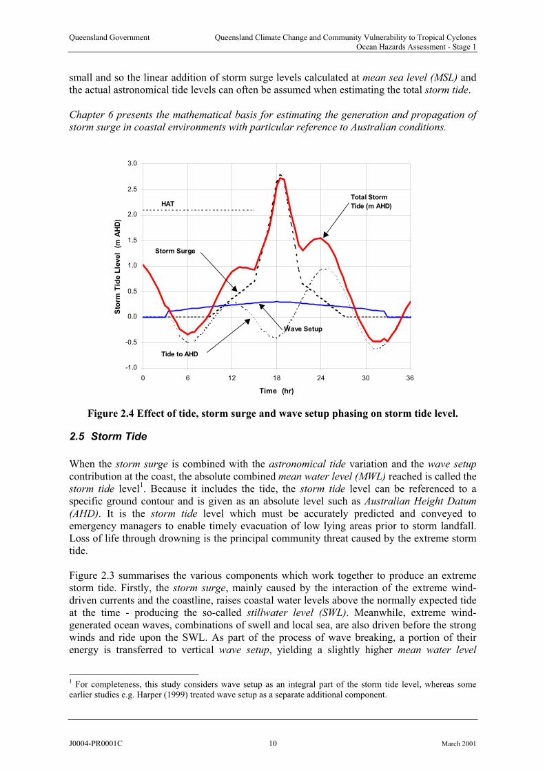
Figure 2.4 Effect of tide, storm surge and wave setup phasing on storm tide level.
2.5 Storm Tide
When the storm surge is combined with the astronomical tide variation and the wave setup
contribution at the coast, the absolute combined mean water level (MWL) reached is called the storm tide level1. Because it includes the tide, the storm tide level can be referenced to a specific ground contour and is given as an absolute level such as Australian Height Datum
(AHD). It is the storm tide level which must be accurately predicted and conveyed to emergency managers to enable timely evacuation of low lying areas prior to storm landfall. Loss of life through drowning is the principal community threat caused by the extreme storm tide.
Figure 2.3 summarises the various components which work together to produce an extremestorm tide. Firstly, the storm surge, mainly caused by the interaction of the extreme wind-driven currents and the coastline, raises coastal water levels above the normally expected tide at the time - producing the so-called stillwater level (SWL). Meanwhile, extreme wind-generated ocean waves, combinations of swell and local sea, are also driven before the strong winds and ride upon the SWL. As part of the process of wave breaking, a portion of their energy is transferred to vertical wave setup, yielding a slightly higher mean water level
1 For completeness, this study considers wave setup as an integral part of the storm tide level, whereas someearlier studies e.g. Harper (1999) treated wave setup as a separate additional component.
J0004-PR0001C 10 March 2001
Queensland Government Queensland Climate Change and Community Vulnerability to Tropical CyclonesOcean Hazards Assessment - Stage 1
(MWL). Additionally, individual waves will run-up sloping beaches to finally expend their forward energy and, when combined with the elevated SWL, this allows them to attack foredunes or nearshore structures to cause considerable erosion or destruction of property.
The principal role of the astronomical tide is then in providing a background modulation in coastal water levels. The relative phasing of the arrival of the storm surge and associated wave setup relative to the tide determines the actual variation in storm tide levels, as illustrated in Figure 2.4. The example shown is similar to the storm tide response duringcyclone Althea in Townsville in 1971, where the peak surge arrived fortunately close to thetime of low tide.
The first critical phase of a storm tide is when the MWL commences to exceed the local Highest Astronomical Tide (HAT), which represents the normal landward extent of the sea at any coastal location (Queensland Transport 1999). By this time, depending on the coastal features, it is likely that extensive beach and dune erosion will have occurred due to waverunup effects alone. If the water level rises further, inundation of normally dry land will commence and the storm tide will be capable of causing loss of life through drowning and significant destruction of nearshore buildings and facilities if large ocean swell penetrate theforeshore regions.
Table 2.2, extracted from Harper (1999), provides a summary of some of the more significant storm tide events known to have occurred in Queensland, caused by tropical cyclones. This list should be regarded as indicative only but shows that at least 34 separate surge events occurred during the past 100 years which resulted in storm tide levels reaching above the HAT level. As significant as this record might appear, it is of little value in estimating thelong-term hazard of storm tide inundation at any specific part of the coastline. Accordingly,extensive numerical and statistical modelling is required to provide the guidance needed forplanning and warning activities.
Chapter 9 addresses techniques for estimating the long-term risk of inundation by storm tide
at any specific coastal location and traces the development of various methods.
Chapter 10 demonstrates the current state-of-the-art ability to reproduce (or hindcast) the
actual storm tides from a selection of historical cyclones on the Queensland coast using the
MMUSURGE modelling system.
J0004-PR0001C 11 March 2001

Queensland Government Queensland Climate Change and Community Vulnerability to Tropical CyclonesOcean Hazards Assessment - Stage 1
Table 2.2 Summary of significant Queensland storm tides.
Reference Storm Storm Inundation
Central Surge Tide Above
Date Place Event Pressure Level HAT
hPa m m AHD m
1858 Green Is ? ? 2? "awash"
04-Mar-1887 Albert R Heads "cyc" 5.5? 7.8 5.1
08-Jun-1891 Brisbane ? ? 1.8 0.3
19-Feb-1894 Brisbane "cyc" 0.6 1.6 0.2
26-Jan-1896 Townsville Sigma "hur" >2? 4? 2?
05-Mar-1899 Bathurst Bay Mahina 914 13.7? 13? 11?
09-Mar-1903 Cairns Leonta 965< ? 2+? 0.7
27-Jan-1910 Cairns "hur" ? 2+? 0.7
21-Jan-1918 Mackay 933 3.8 5.5 2
10-Mar-1918 Mission Beach 926 >7? 8? 3.5?
04-Feb-1920 Cairns 988 >1.5 2.5? 0.7?
30-Mar-1923 Albert R Heads Douglas Mawson 974 >3 5? 2.3?
16-Jun-1928 Brisbane ? ? 1.7 0.2
11-Mar-1934 Cape Tribulation 968 >9? >7? >6?
17-Mar-1945 Cairns 994 >0.8 ? ?
28-Jan-1948 Brisbane ? 0.5 1.8 0.3
23-Feb-1948 Bentinck Is 996 >3.7 4.7? 3.2?
02-Mar-1949 Gladstone 988 >1.2 2.2 0.2
18-Jan-1950 Brisbane ? 0.6 1.8 0.3
21-Feb-1954 Coolangatta 973 >1? 2? ?
03-Feb-1964 Edward River Dora 974 5? ? ?
29-Jan-1967 Moreton Bay Dinah 945 2? 2.8? 1.5?
19-Feb-1971 Inkerman Station Fiona 960 >4? ? ?
24-Dec-1971 Townsville Althea 952 2.9 2.6 0.4
11-Feb-1972 Fraser Island Daisy 959 3? ? ?
07-Feb-1974 Brisbane Pam 965 0.7 1.9 0.4
19-Dec-1976 Albert River Ted 950 4.6? 6.3? 3.6?
31-Dec-1978 Weipa Peter 980 1.2 2.3 0.6
26-Apr-1989 Beachmere Charlie 972 0.6 1.5 0.2
04-Apr-1989 Molongle Creek Aivu 935 3.2? 3.7? 1.7?
16-Mar-1992 Burnett Heads Fran 980 1 2.1 0.2
06-Jan-1996 Gilbert River Barry 950 4.5? 6? 3.4?
09-Mar-1996 Weipa Ethel 980 1.2 3.6 0.3
08-Mar-1997 Cairns Justin 975 0.7 1.9 0.2
27-Feb-2000 Cairns Steve 975 0.99 1.07 -
3-Apr-2000 Townsville Tessi 980 1.05 1.73 -
J0004-PR0001C 12 March 2001

Queensland Government Queensland Climate Change and Community Vulnerability to Tropical CyclonesOcean Hazards Assessment - Stage 1
2.6 References
BoM (1999) Tropical cyclone warning directive (eastern region) 1999-2000. Queensland Regional Office, Bureau of Meteorology.
Harper B.A. (1999) Storm tide threat in Queensland: History, prediction and relative risks. Conservation Technical Report No. 10, Dept of Environment and Heritage, Jan, ISSN 1037-4701.
Holland G.J. (1997) The maximum potential intensity of tropical cyclones. J. Atmos. Sci., 54, Nov, 2519-2541.
Queensland Transport (1999) The official tide tables and boating safety guide 2000. Queensland Department of Transport.
Wakimoto W. and Black P.G. (1994) Damage survey of Hurricane Andrew and its relationship to the eyewall. Bull. Amer. Met. Soc., 75 (2), 189-200.
WMO (1995) Global perspectives on tropical cyclones. TD-No. 693, Tropical Cyclone Programme Report No. TCP-38, World Meteorological Organization, Geneva.
WMO (1997) Tropical cyclone operational plan for the South Pacific and South-East Indian Ocean. TD-No. 292, Tropical Cyclone Programme Report No. TCP-24, World
Meteorological Organization, Geneva.
J0004-PR0001C 13 March 2001
Queensland Government Queensland Climate Change and Community Vulnerability to Tropical CyclonesOcean Hazards Assessment - Stage 1
3. Tropical Cyclone Climatology of Queensland
3.1 Historical Summary of Incidence and Intensity
Recent historical research into the impacts of tropical cyclones affecting the Queenslandregion has uncovered significant community impacts as early as the mid-1800s (Callaghan 2000). The most significant impact recorded to date is the 1889 "Mahina" or "Bathurst Bay"cyclone (Whittingham 1958) which destroyed a pearling fleet in Princess Charlotte Bay with the loss of over 300 lives. The 914 hPa central pressure attributed to this event is based on a reading of 27" Hg from a schooner that was almost sunk and, if accurate, represents a recordintensity for landfalling cyclones on the Queensland coast. The storm is also reported to have produced a massive storm surge of the order of 12 m (refer Table 2.2 entry), although that is less supportable based on present-day surge estimation techniques. A recent site debris survey (Nott and Hayne, 2000) has also failed to confirm evidence of such a significant surge event and it is concluded for the moment that wave runup may have been a significant contributor to the historical account. Nevertheless, the 1899 cyclone remains as an extreme example of the potential severity of tropical cyclones impacting the Queensland coast.
The official tropical cyclone record maintained in electronic form by the Bureau ofMeteorology National Climate Centre (NCC) begins in the 1906/07 season. This database derives from climatological summaries by Coleman (1972) and later Lourensz (1977, 1981) with updates of "best track" information from the Regional Offices since that time. An overview of this 94 year official record is given below, summarising cyclone activity within aradius of 1500 km from Mackay, which includes all cyclones that entered the 138ºE to 160ºE jurisdictional area of the Queensland Regional Office2. A complete summary of all stormdetails is included as Appendix B.
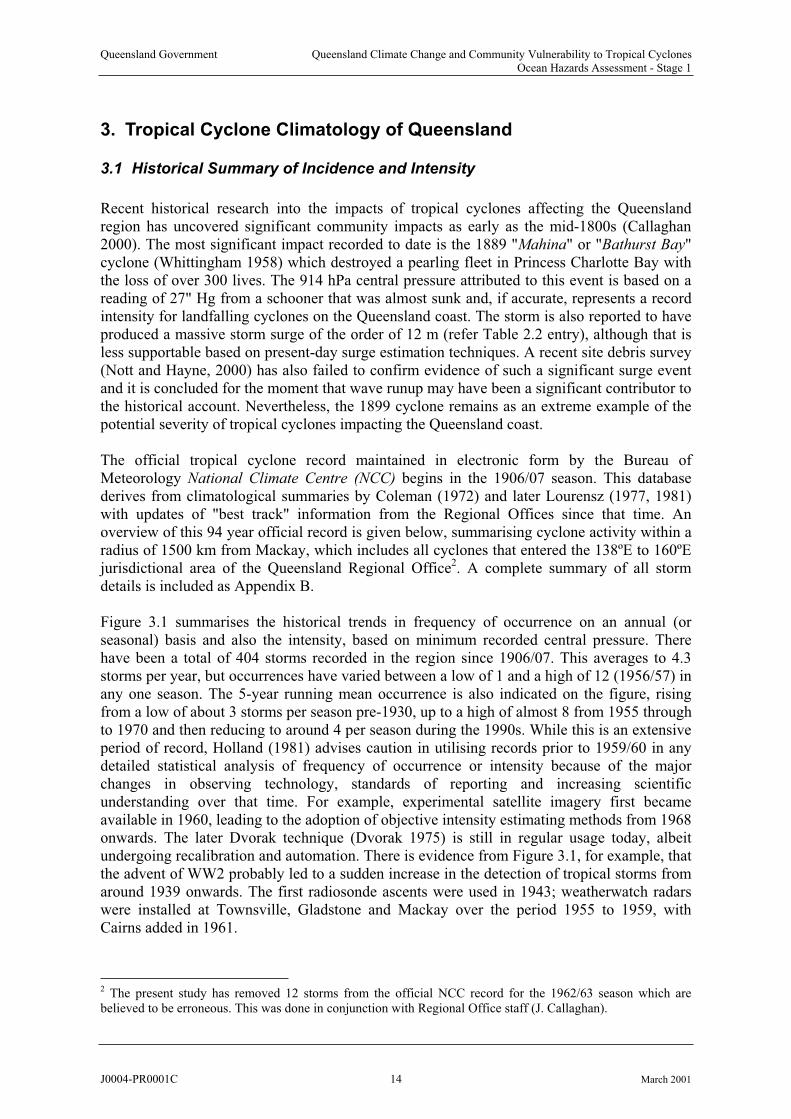
Figure 3.1 summarises the historical trends in frequency of occurrence on an annual (or seasonal) basis and also the intensity, based on minimum recorded central pressure. Therehave been a total of 404 storms recorded in the region since 1906/07. This averages to 4.3 storms per year, but occurrences have varied between a low of 1 and a high of 12 (1956/57) in any one season. The 5-year running mean occurrence is also indicated on the figure, rising from a low of about 3 storms per season pre-1930, up to a high of almost 8 from 1955 through to 1970 and then reducing to around 4 per season during the 1990s. While this is an extensive period of record, Holland (1981) advises caution in utilising records prior to 1959/60 in any detailed statistical analysis of frequency of occurrence or intensity because of the majorchanges in observing technology, standards of reporting and increasing scientific understanding over that time. For example, experimental satellite imagery first becameavailable in 1960, leading to the adoption of objective intensity estimating methods from 1968 onwards. The later Dvorak technique (Dvorak 1975) is still in regular usage today, albeit undergoing recalibration and automation. There is evidence from Figure 3.1, for example, that the advent of WW2 probably led to a sudden increase in the detection of tropical storms from around 1939 onwards. The first radiosonde ascents were used in 1943; weatherwatch radars were installed at Townsville, Gladstone and Mackay over the period 1955 to 1959, with Cairns added in 1961.
2 The present study has removed 12 storms from the official NCC record for the 1962/63 season which arebelieved to be erroneous. This was done in conjunction with Regional Office staff (J. Callaghan).
J0004-PR0001C 14 March 2001
Queensland Government Queensland Climate Change and Community Vulnerability to Tropical CyclonesOcean Hazards Assessment - Stage 1
0
2
4
6
8
10
12
14
1905 1915 1925 1935 1945 1955 1965 1975 1985 1995
Season
Num
ber
of
Cyclo
nes P
er
Year
0
50
100
150
200
250
300
350
400
450
500
Tota
l N
um
ber
of
Cyclo
nes
5 yr Av
910
920
930
940
950
960
970
980
990
1000
1010
1905 1915 1925 1935 1945 1955 1965 1975 1985 1995
Season
Min
imu
mC
en
tra
l P
ressu
re (
hP
a)
5 yr Av
Figure 3.1 Historical trends for tropical cyclones in the Queensland region
J0004-PR0001C 15 March 2001

Queensland Government Queensland Climate Change and Community Vulnerability to Tropical CyclonesOcean Hazards Assessment - Stage 1
Offshore automatic weather stations (AWS) were then gradually installed from 1970 onwards, initially at Flinders Reef and Lihou Reef, followed by Creal Reef, Gannet Cay and HolmesReef in 1972. Prior to this time the staffed Willis Island station provided the only fixed remote offshore observations. Routine infrared satellite observations only became available in1972 and geostationary satellites in 1978 provided fixed reference points.
The time series of minimum storm central pressure underpins the need for caution in selecting a representative period for statistical analysis. With the exception of the influence of the 1918 season, which witnessed two very severe landfalling storms (Mackay and Innisfail), the 5-year average central pressures rarely fell below 980 hPa until the late 1960s, when the early Dvorak technique was becoming established. From then until the early 1990s, the incidence of more intense storms continued to increase and the average pressure fell to a low of 955 hPa, before rising again over the past decade. The extent to which this variability is entirely due toclimate or due to interpretation and classification remains unknown. However, the availability of satellite data clearly had a considerable impact at least in detection of the systems. The degree to which satellite influenced classification is perhaps harder to assess, although adoption of the newly developing intensity estimation methods was probably gradual and there may still be a bias towards lower intensities over the first decade after its introduction.For example, Callaghan (2000) suggests there may have been a reluctance amongst manyforecasters to "overstate" a storm's intensity without reasonable groundtruth being available,even as late as the mid-1970s. If such a bias exists, then it is probably more pronounced furthest from the coast or in the more remote regions. The quantitative data quality assessmentby Holland (1981) is summarised in Table 3.1 for the Eastern Region (nominally 142ºE to 165ºE). Here "coastal" refers to < 500 km of the coast and "Group 1" refers to situations with an observation within 100 km and 12 h of the place and time of maximum intensity. Hisanalysis concludes the possibility of at least 10 to 15 hPa errors in estimating intensity over the period 1959 to 1979.
Table 3.1 Data base quality assessment for the Eastern Region (after Holland 1981)
Statistic Situation 1909-1939 1939-1959 1959-1969 1969-1979
Occurrence: Coastal 15% to 30% low 5% to 15% low < 5% low < 5% low
Open Ocean > 50% low > 50% low 15% to 30% low < 5% low
Coast Crossing: 5% to 15% low < 5% low < 5% low < 5% low
Location Accuracy: Coastal < 250 km < 150 km <100 km < 50 km
Open Ocean no idea < 250 km 150 - 100 km <100 km
Intensity: Group 1 < 15 hPa < 15 hPa < 15 hPa < 10 hPa
Group 2 no idea no idea < 30 hPa < 20 hPa
Another source of bias which is known to exist in the historical data is the inclusion of some"winter cyclones", which have a Category 1 level of severity and would now be classed as east coast lows. Their inclusion in the tropical cyclone dataset would tend to increase the apparent frequency of tropical cyclones but also reduce the average intensity estimates.
3.2 Statistical Analysis of Post 1959/60 Data
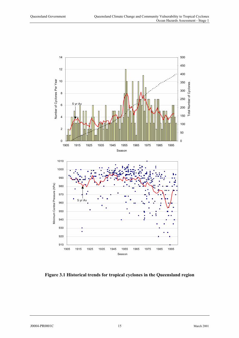
Restricting the data set to post-1959/60 more than halves the available record but results in a total of 213 storms in a 41 year period, giving an average occurrence rate of 5.2 per season, an increase of more than one per year compared with the full record. Figure 3.2 shows the basic occurrence statistics and intensity histogram for this reduced dataset.
J0004-PR0001C 16 March 2001
Queensland Government Queensland Climate Change and Community Vulnerability to Tropical CyclonesOcean Hazards Assessment - Stage 1
0
5
10
15
20
25
30
1959 1964 1969 1974 1979 1984 1989 1994 1999
Season
Num
ber
of
Cyclo
nes P
er
Year
-25
-20
-15
-10
-5
0
5
10
15
20
25
Annual S
OI
Valu
eA
nnual IP
Ox 1
0
SOI Annual
SOI 5 yr
IPO Annual
5 yr Av
0
5
10
15
20
25
900 910 920 930 940 950 960 970 980 990
Central Pressure (hPa)
% C
yclo
nes
0
10
20
30
40
50
60
70
80
90
100
Cum
ula
tive %
Figure 3.2 The post-1959/60 tropical cyclone dataset for Queensland.
J0004-PR0001C 17 March 2001
Queensland Government Queensland Climate Change and Community Vulnerability to Tropical CyclonesOcean Hazards Assessment - Stage 1
0
2
4
6
8
10
12
14
0 24 48 72 96 120 144 168 192 216 240 264 288 312
Storm Duration (h)
% o
fC
yclo
nes
0
10
20
30
40
50
60
70
80
90
100
Cum
ula
tive %
0
5
10
15
20
25
30
35
Aug Sep Oct Nov Dec Jan Feb Mar Apr May Jun Jul
Starting Month
% o
f C
yclo
nes
0
10
20
30
40
50
60
70
80
90
100
Cum
ula
tive %
Figure 3.3 Tropical cyclone seasonal occurrence and duration post 1959/60.
J0004-PR0001C 18 March 2001
Queensland Government Queensland Climate Change and Community Vulnerability to Tropical CyclonesOcean Hazards Assessment - Stage 1
0
5
10
15
20
25
30
35
0 2 4 6 8 10 12 14
Forward Speed (m/s)
% o
f C
yclo
nes
0
10
20
30
40
50
60
70
80
90
100
Cum
ula
tive %
0
1
2
3
4
5
6
7
8
9
0 30 60 90 120 150 180 210 240 270 300 330
Track Bearing (deg)
% o
f C
yclo
nes
0
10
20
30
40
50
60
70
80
90
100
Cum
ula
tive %
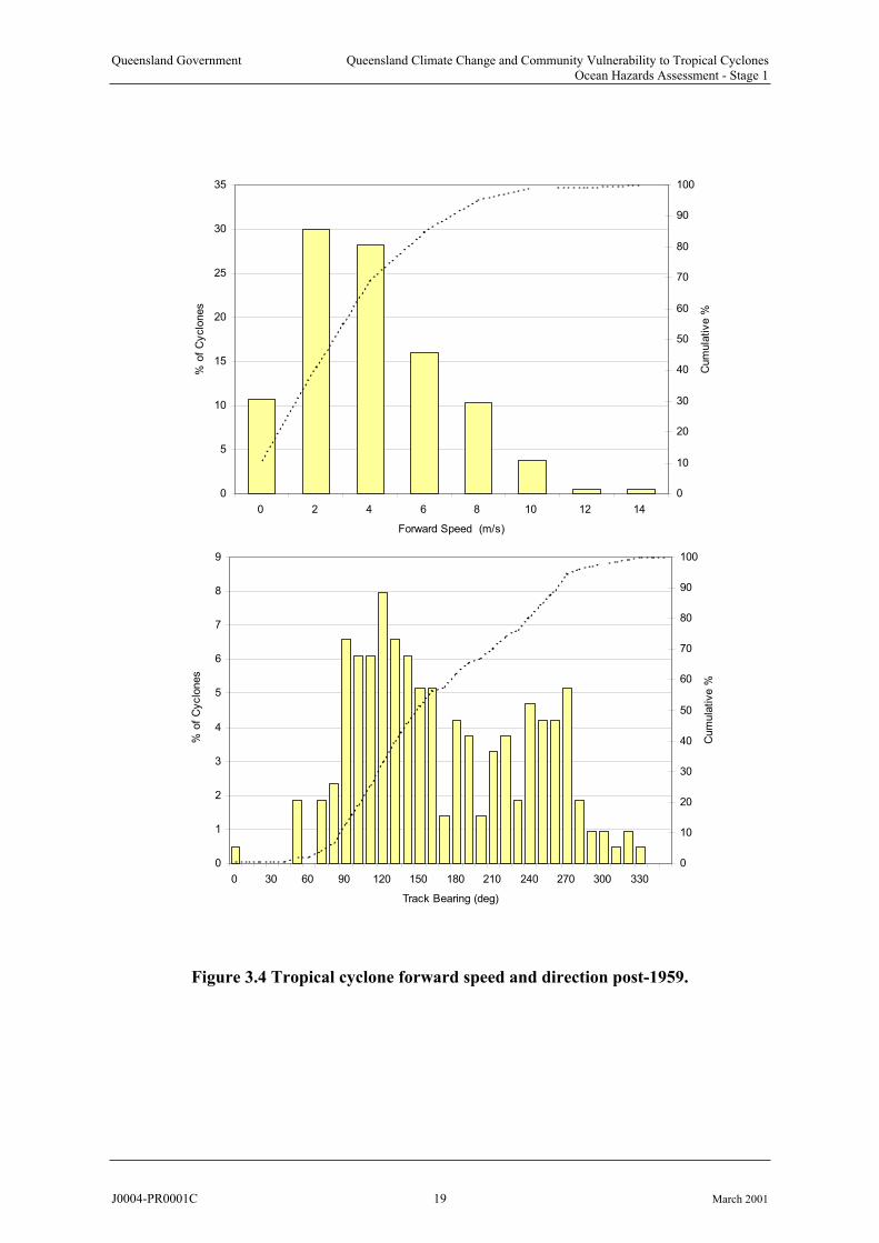
Figure 3.4 Tropical cyclone forward speed and direction post-1959.
J0004-PR0001C 19 March 2001
Queensland Government Queensland Climate Change and Community Vulnerability to Tropical CyclonesOcean Hazards Assessment - Stage 1
Cairns •
Weipa •
Cooktown •
Townsville •
Mackay •
Gladstone •
Noosa •Brisbane •
Karumba •
140ºE 150ºE 160ºE
30ºS
20ºS
10ºS
Hervey Bay •
Rockhampton •
Cairns •
Weipa •
Cooktown •
Townsville •
Mackay •
Gladstone •
Noosa •Brisbane •
Karumba •
140ºE 150ºE 160ºE
30ºS
20ºS
10ºS
Hervey Bay •
Rockhampton •
Cairns •
Weipa •
Cooktown •
Townsville •
Mackay •
Gladstone •
Noosa •Brisbane •
Karumba •
140ºE 150ºE 160ºE
30ºS
20ºS
10ºS
Hervey Bay •
Rockhampton •
Cairns •
Weipa •
Cooktown •
Townsville •
Mackay •
Gladstone •
Noosa •Brisbane •
Karumba •
140ºE 150ºE 160ºE
30ºS
20ºS
10ºS
Hervey Bay •
Rockhampton •
November December
Cairns •
Weipa •
Cooktown •
Townsville •
Mackay •
Gladstone •
Noosa •Brisbane •
Karumba •
140ºE 150ºE 160ºE
30ºS
20ºS
10ºS
Hervey Bay •
Rockhampton •
January February
April
Cairns •
Weipa •
Cooktown •
Townsville •
Mackay •
Gladstone •
Noosa •Brisbane •
Karumba •
140ºE 150ºE 160ºE
30ºS
20ºS
10ºS
Hervey Bay •
Rockhampton •
March
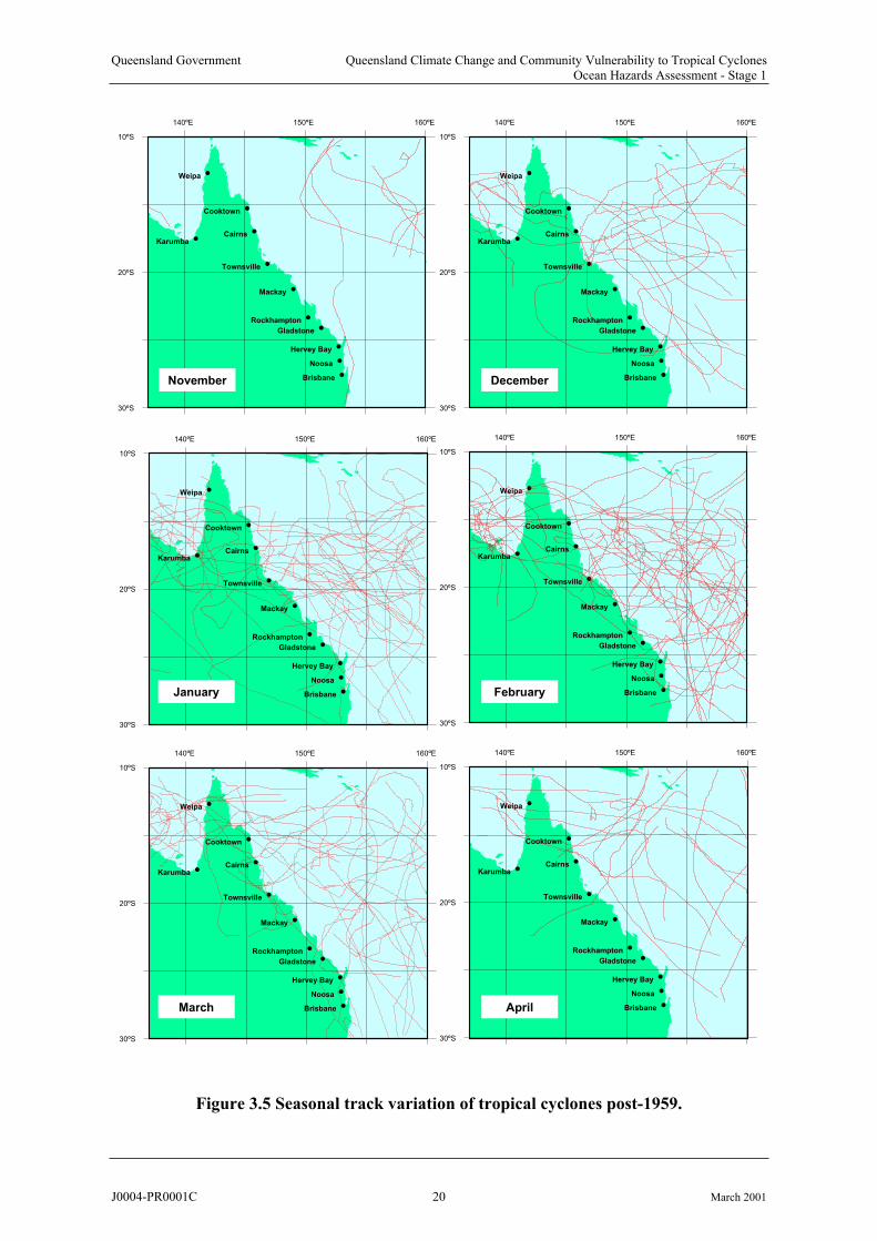
Figure 3.5 Seasonal track variation of tropical cyclones post-1959.
J0004-PR0001C 20 March 2001

Queensland Government Queensland Climate Change and Community Vulnerability to Tropical CyclonesOcean Hazards Assessment - Stage 1
Figure 3.2 also shows time history comparisons against the annual and 5 year averaged Southern Oscillation Index (SOI) and the Inter-decadal Pacific Oscillation (IPO). Further discussion on these points is provided later in regard to climatic variability.
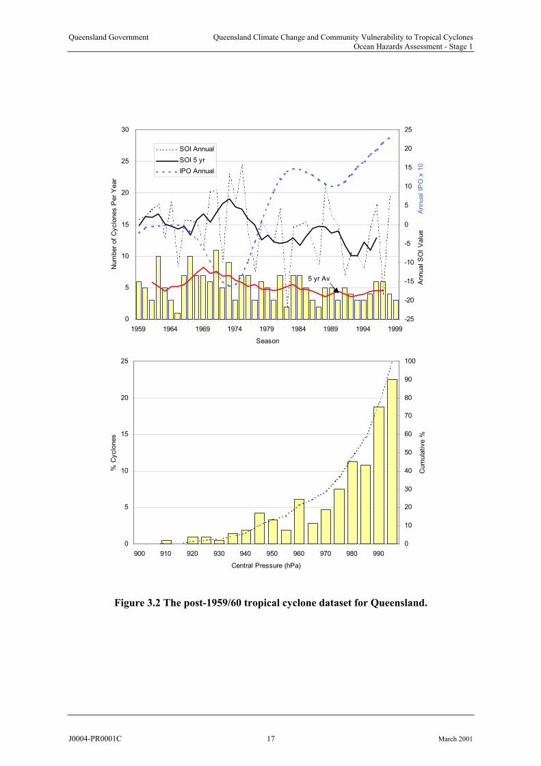
Figure 3.3 shows the seasonal analysis of cyclone start date by month, indicating mosttropical cyclones in the region (83%) occur during the period from December through to March, although November with 4.7% of the total is acknowledged as the start of the season. February can be seen to have the highest proportion at 28%, followed by January with 24% and March with about 20%. December and April are similar with only 10% and 8% respectively. The small incidence in May mainly represents dataset contamination from eastcoast lows, as mentioned previously.
The histogram of duration shows that cyclone lifetimes can be highly variable. Approximately60% of all cyclones exist for less than 4 days, but 10% may persist for 8 days or more. This variation is dictated to a large extent by the forward speed and track of individual storms, assummarised at the time of their maximum intensity in Figure 3.4. In this case the most likely forward speed is about 2 m s-1, with the average being about 3 m s-1. The very highest speeds (> 10 m s-1) are normally associated with those cyclones undergoing extra-tropical transition at higher latitudes.
The distribution of track bearing (direction towards) at time of maximum intensity showspredominance in the E to SSE band, peaking near SE and tending to represent the shape of the east coast. There are also other bands near the SSW and between SW and W. After theirformation in low latitudes, cyclones tend to move westwards and polewards under combinedeasterly steering currents and dynamical effects, although individual tracks can be erratic. South of latitude 15°S on the Queensland coast, the major direction of movement is southeastward. This is caused by interaction with the northwesterly winds to the east of deep mid-latitude troughs that tend to steer tropical cyclones southeastward parallel to the coast (Callaghan 2000). The continental east coast itself participates in this process by influencing the evolution and structure of these trough systems. As tropical cyclones move into temperatelatitudes they begin to interact with troughs in the middle to upper westerlies. There are three possibilities in South East Queensland as a result of this interaction. The cyclone may remainsufficiently removed from the westerlies to retain tropical cyclone characteristics; thewesterlies may interfere destructively with the cyclone circulation and weaken it or thecyclone may interact favourably with an upper trough to form an intense temperate latitude cyclone – collectively termed extra-tropical cyclones in the literature. These processes, combined with unfavourable SST, tend to place a limit on the southerly extent of severe tropical cyclones.
Figure 3.5 provides an overview of tracks in the Queensland region, summarised on the basis of the starting month. The season can be seen to develop in all areas as the season progresses,although by April the activity in the Gulf of Carpentaria appears to have reduced significantly. January appears to have the greatest proportion of overland tracks, principally being sourced from the Gulf region.
Although the tracks of Figure 3.5 appear essentially randomised, it is possible to undertakesystematic statistical analyses to yield summary parameters that can be used in risk assessment studies. The results from one such analysis (after Harper 1999) are given in Figure 3.6. The technique applied in this case is to analyze samples of track parameters within a given radius (500 km) of a number of coastal locations - which are indicated on the figure.
J0004-PR0001C 21 March 2001

Queensland Government Queensland Climate Change and Community Vulnerability to Tropical CyclonesOcean Hazards Assessment - Stage 1
(b) Cyclone Occurrence
0.0
0.5
1.0
1.5
2.0
2.5
3.0
-28-26-24-22-20-18-16
Latitude (deg)
Fre
qu
en
cy
of
Sto
rms p
er
Year Offshore Moving
Parallel to Coast
Coast Crossing
All Classes
(a) Cyclone Intensity
890
900
910
920
930
940
950
960
970
980
-28-26-24-22-20-18-16
Latitude (deg)
Ce
ntr
al P
res
su
re (
hP
a)
10 y
50 y
100 y
500 y
Bri
sb
an
e
He
rve
y B
ay
Gla
ds
ton
e
Ma
ck
ay
To
wn
sv
ille
Ca
irn
s
MPI
Figure 3.6 Smoothed statistical analyses of post-1959 tropical cyclone track data
(based on a 500 km radius at each 2 latitude ; analyses after Harper 1999).
J0004-PR0001C 22 March 2001

Queensland Government Queensland Climate Change and Community Vulnerability to Tropical CyclonesOcean Hazards Assessment - Stage 1
Firstly, an extreme value analysis of the minimum central pressures yields a latitudinal variation in intensity, peaking in the vicinity of Mackay. Curves are shown for average returnperiods of 10, 50, 100 and 500 y applicable to the 500 km radius sample zones. These are limited by an assumed MPI curve (Holland 1997, pers. comm.) which lies close to the 500 y intensity curve north of Mackay, but reduces to the 100 y curve nearer to Brisbane. Clearly, different return period variations will be obtained with different sample radii. The choice ofradii in this case being guided by the need to maintain an adequate data set for analysis but also to ensure capture of those storms which could affect the central location within 24 h.
Using the same sampling concept, but separating the cyclones into population classes based on characteristic paths, Figure 3.6b shows how the various track class contributions vary with latitude. The "offshore moving" class tends to decrease towards the south, while the "parallelto coast" tends to be relatively small north of Townsville, rising to a peak near Mackay and then staying relatively constant as far south as Hervey Bay. The "coast crossing" class tends to decrease slowly towards the south. The combined threat from tropical cyclones at any point along the coast is then a combination of the frequency of occurrence and the intensity variation. On this basis the Townsville - Mackay region tends to represent the greatest risk.
It should be noted that the available cyclone database is deficient in the recording of horizontal scale information, such as radius to maximum wind estimates and wind peakedness. Accordingly, present hazard assessment studies need to develop statisticaldescriptions of such parameters.
3.3 Climatic Variability
Figure 3.2 shows that the incidence of tropical cyclones can be quite variable from one year to the next and this is because of the complex set of factors that influence their genesis (WMO1995). The data also suggests changes that are associated more with a decadal timescale. In Figure 3.7, for example, the distribution of tracks is shown for each of the decades since1959/60, where there are some strong differences evident. For example, the 1969-1978 decade appears to have many more coastal crossings than the preceding and following periods. Also,the later 1989-1999 period shows a marked decrease in activity south from Townsville.
For many years one of the most frequently used indicators of seasonal cyclonic activity has been the so-called El Niño - Southern Oscillation (ENSO) phenomenon (Nicholls 1992). This is the name given to a near-periodic (between one and three year) cycle of alternating cold and warm ocean temperatures between one side of the Pacific Ocean and the other. The El Niño phase sees abnormally warm ocean temperatures off the coast of South America and along the central and eastern Pacific equatorial zone and simultaneously cooler oceantemperatures in the western Pacific and the Coral Sea. During the reverse cycle, or La Niña,ocean temperatures near the Queensland coast are typically above average. Ocean temperature is not the only factor causing cyclone variability but it is a prime contributor. When combined with associated shifts in large-scale zones of atmospheric convergence (Basher and Zheng 1995), the regions of tropical cyclone genesis in the South Pacific tend, as a result, to movefurther towards the east (El Niño) or the west (La Niña).
There are several techniques used for determining the state or strength of the ENSO condition. One of the most widely used methods is the Southern Oscillation Index (SOI), whichcompares differences in the mean monthly sea level pressure between Darwin and Tahiti. Theannual and 5-year averaged SOI time series is shown in Figure 3.2, compared with the
J0004-PR0001C 23 March 2001

Queensland Government Queensland Climate Change and Community Vulnerability to Tropical CyclonesOcean Hazards Assessment - Stage 1
occurrence of tropical cyclones in the Queensland region. The SOI has been shown to be astrong indicator of rainfall and tropical cyclone activity in northern Australia and Queensland (e.g. Nicholls, 1992). Another common method is to use ocean surface temperature readings(SSTs) from various zones in the Pacific. These data have become routinely available from satellite as well as ships, drifting buoys and from moored buoy networks positioned along the equator. Using an accepted SST-based sequence from 1959 to 1997 (e.g. from Pielke andLandsea, 1999), Figure 3.8 shows that when the historical record is separated into El Niño, neutral and La Niña periods, there is a quite noticeable effect on the tracks of tropicalcyclones in the Coral Sea. During La Niña (the positive SOI phase) cyclone activity tends tobe located closer to the east coast of Queensland and further south than during the El Niño (negative SOI phase). The Gulf of Carpentaria appears to be less affected.
While the ENSO phenomenon appears to be somewhat random, El Niño years have outnumbered La Niña years by about a factor of 3 since the mid-1970s. This has been reflected along much of the east coast of Queensland by a corresponding reduction in frequency of cyclone occurrence and Figure 3.2 indicates this effect from the 1970s onwards, which becomes much magnified if only the area south of Mackay is considered. Exactly why this preference for El Niño episodes has persisted during this period is not entirely clear but itmay be related to longer period climatic variability as discussed below, or even global climatechange. From 1998 to early 2000 there has been a return to mild La Niña and near-neutral conditions. Latest SOI results (Nov-Dec 2000) suggest a stronger La Niña could be developing for 2001.
Interestingly, as shown in the following table, neutral years actually have the highest frequency of occurrence of cyclones in the Queensland region, although the number of ElNiño, neutral and La Niña years is approximately equal over the 41 year record. Numbers of neutral years alone account for nearly 40% of all occurrences. Importantly, neutral years show a 53% increase in occurrences compared with El Niño years and a 5.5% increase compared with La Niña years.
Table 3.2 Summary ENSO statistics for Queensland.
ENSOCondition
YearsExperienced
Total CycloneNumbers
Frequency of Occurrence
Proportion of Occurrences
El Niño 14 55 3.93 25.8%
Neutral 14 84 6.00 39.4%
La Niña 13 74 5.69 34.7%
Total 41 213 5.20 100%
Power et al. (1999) recently highlighted the potential importance for Australian climate of apparent 10 to 30 year longer-term cycles of ocean temperatures in the Pacific Ocean. This oscillation is also measured in terms of relative SST heating or cooling but relates more to thewhole of the tropical Pacific Ocean region rather than just differences between the eastern and western limits. Termed the Inter-decadal Pacific Oscillation (IPO), this long-term variation inmean SST appears to modulate the effect of ENSO on rainfall in Australia. When the IPO is positive, the tropical ocean is slightly warmer than average while to the north and south the temperatures are slightly less than average. During this period the effect of ENSO on rainfallappears to be less significant. When the IPO is “negative”, the tropical ocean is slightly coolerand ENSO seems to be much more strongly correlated with Australian rainfall. The IPO effect
J0004-PR0001C 24 March 2001

Queensland Government Queensland Climate Change and Community Vulnerability to Tropical CyclonesOcean Hazards Assessment - Stage 1
Cairns •
Weipa •
Cooktown •
Townsville •
Mackay •
Gladstone •
Noosa •Brisbane •
Karumba •
140ºE 150ºE 160ºE
30ºS
20ºS
10ºS
Hervey Bay •
Rockhampton •
Cairns •
Weipa •
Cooktown •
Townsville •
Mackay •
Gladstone •
Noosa •Brisbane •
Karumba •
140ºE 150ºE 160ºE
30ºS
20ºS
10ºS
Hervey Bay •
Rockhampton •
1959-1968 1969-1978
Cairns •
Weipa •
Cooktown •
Townsville •
Mackay •
Gladstone •
Noosa •Brisbane •
Karumba •
140ºE 150ºE 160ºE
30ºS
20ºS
10ºS
Hervey Bay •
Rockhampton •
Cairns •
Weipa •
Cooktown •
Townsville •
Mackay •
Gladstone •
Noosa •Brisbane •
Karumba •
140ºE 150ºE 160ºE
30ºS
20ºS
10ºS
Hervey Bay •
Rockhampton •
1979-1988 1989-1999
Figure 3.7 Decadal tropical cyclone track variability post-1959.
may also be related to the large-scale thermo-haline circulation between the Atlantic and the Pacific Ocean that has been identified as a potential indicator of hurricane incidence in theAtlantic (Landsea et al., 1994). Callaghan and Power (submitted AMM) describe a possible modulating effect of the IPO on Australian tropical cyclone activity which suggests that damaging impacts in Queensland are more likely during negative (cooler) phases of the IPO,which is associated with warmer ocean temperatures near Queensland. Since the mid-1970s,there has been a prolonged positive phase of the IPO that is only now (1999-2000) showing some possible signs of reversal. If this is correct, recent trends may suggest that cyclone incidences along the Queensland coast could increase, especially in the SE region. However, these outcomes remain speculative at this time since it will require several further years of observations to confirm whether the IPO phase is changing. The annual IPO index x 10 is plotted as a time series in Figure 3.2 for comparison with the SOI and cyclone occurrences.Generally the IPO can be seen to inversely mimic the SOI, except from around 1985 to 1990 where the IPO failed to reverse when the SOI rose and it is now thought the IPO is at or near its peak positive phase.
J0004-PR0001C 25 March 2001
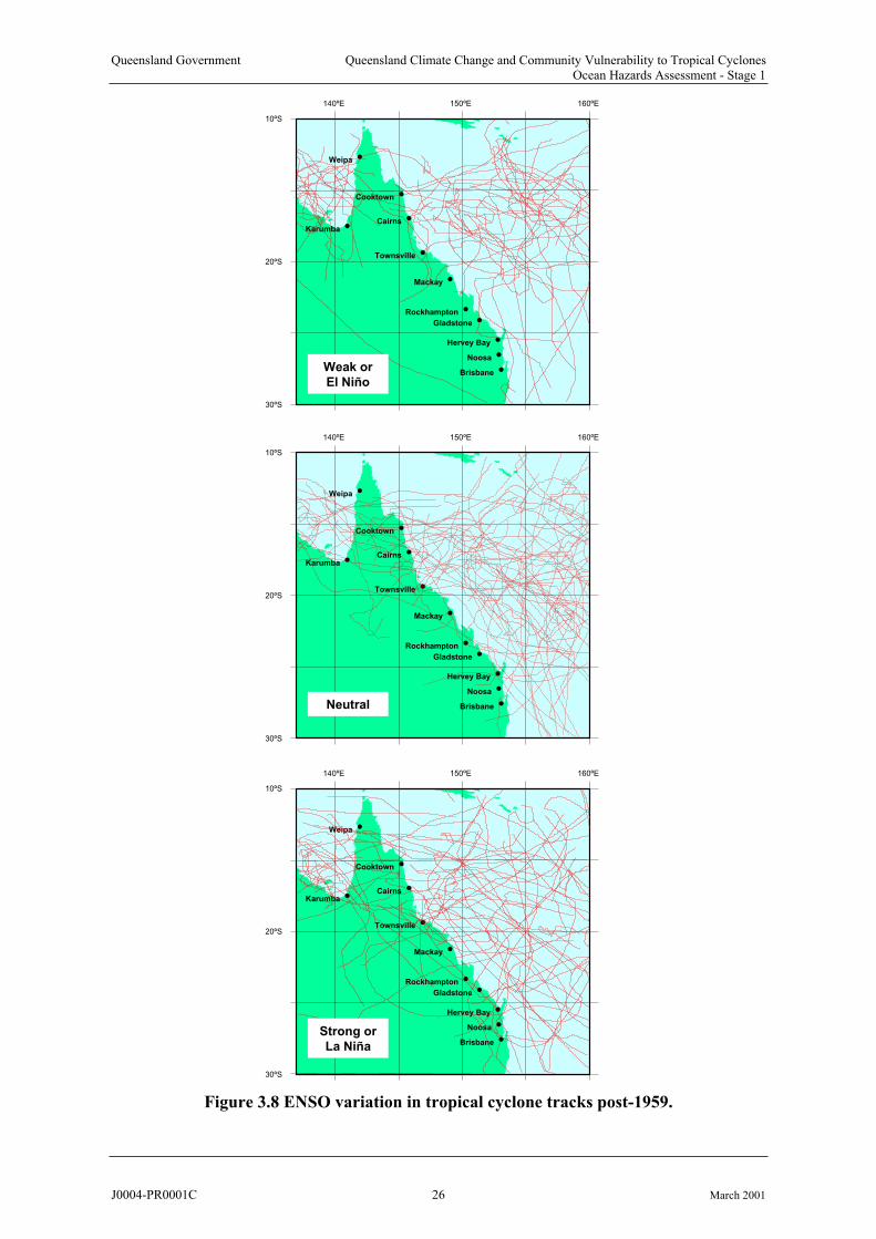
Queensland Government Queensland Climate Change and Community Vulnerability to Tropical CyclonesOcean Hazards Assessment - Stage 1
Cairns •
Weipa •
Cooktown •
Townsville •
Mackay •
Gladstone •
Noosa •Brisbane •
Karumba •
140ºE 150ºE 160ºE
30ºS
20ºS
10ºS
Hervey Bay •
Rockhampton •
Cairns •
Weipa •
Cooktown •
Townsville •
Mackay •
Gladstone •
Noosa •Brisbane •
Karumba •
140ºE 150ºE 160ºE
30ºS
20ºS
10ºS
Hervey Bay •
Rockhampton •
Weak or
El Niño
Strong or
La Niña
Cairns •
Weipa •
Cooktown •
Townsville •
Mackay •
Gladstone •
Noosa •Brisbane •
Karumba •
140ºE 150ºE 160ºE
30ºS
20ºS
10ºS
Hervey Bay •
Rockhampton •
Neutral
Figure 3.8 ENSO variation in tropical cyclone tracks post-1959.
J0004-PR0001C 26 March 2001
Queensland Government Queensland Climate Change and Community Vulnerability to Tropical CyclonesOcean Hazards Assessment - Stage 1
3.4 Conclusions and Recommendations
Any assessment of ocean hazards due to the effects of tropical cyclones in Queensland needs to assimilate the many climatological factors that affect cyclone frequency and intensity, on a variety of time and space scales. However, errors and inaccuracies exist in the availabledatasets (this includes the "official" national Climate Centre records) and not all of the necessary information is readily available. This requires development of robust statistical models of the climatology that can be applied in hazard assessments and provide the meansfor sensitivity testing of the many necessary assumptions.
It is recommended that a complete review of tropical cyclone climatology be undertaken for
Queensland that can be used to support future stages of the present ocean hazard assessment
project. This should include inter-seasonal, inter-decadal and long-term climate change
issues. Synoptic scale interactions with tropical cyclone vortices should also be considered,
together with decay after landfall, recurvature and regeneration issues.
3.5 References
Basher R.E. and Zheng X. (1995) Tropical cyclones in the Southwest Pacific: spatial patterns and relationships to southern oscillation and sea surface temperature, Journal of Climate, Vol 8, May, 1249-1260.
Callaghan J. and Power, S. (to appear) Long term changes in the occurrence of damagingcyclonic storms in tropical and sub tropical eastern Australia. Submitted Aust. Met. Magazine
1999.
Coleman F. (1972) Frequencies, tracks and intensities of tropical cyclones in the Australian region, 1909 - 1969. Bureau of Meteorology, Meteorological Summary. July.
Dvorak V.F. (1975) Tropical cyclone intensity analysis and forecasting from satellite imagery. Mon. Weath. Rev., 103, 420-430.
Harper B.A. (1999) Numerical modelling of extreme tropical cyclone winds. APSWE SpecialEdition, Journal of Wind Engineering and Industrial Aerodynamics, 83, 35 - 47.
Holland G.J. (1981) On the quality of the Australian tropical cyclone data base. Aust. Met.
Mag., 29, 169-181.
Holland G.J. (1997) The maximum potential intensity of tropical cyclones. J. Atmos. Sci., 54, Nov, 2519-2541.
Lourensz R.S. (1977) Tropical Cyclones in the Australian Region July 1909 to June 1975. Bureau of Meteorology.
Lourensz R.S. (1981) Tropical cyclones in the Australian region July 1909 to June 1980. Bureau of Meteorology. Oct.
Nicholls N. (1992) Historical El Nino / Southern Oscillation variability in the Australian region. In Diaz, H.F. and Margraf, V. (Eds), El Nino, historical and paleoclimate aspects of the Southern Oscillation. Cambridge Uni. Press, Cambridge, UK, 51-174.
J0004-PR0001C 27 March 2001
Queensland Government Queensland Climate Change and Community Vulnerability to Tropical CyclonesOcean Hazards Assessment - Stage 1
Nott J. and Hayne M. (2000) How high was the storm surge from tropical cyclone Mahina?Aust Jnl of Emergency Management, Autumn, 11-13.
Pielke R.A. (Jr) and Landsea C.W. (1999) La Niña, El Niño, and Atlantic hurricane damagesin the United States, Bull. Amer. Meteor. Soc., 80, 2027-2033.
Power S., Casey T., Folland C., Colman A. and Mehta V. (1999) Inter-decadal modulation of the impact of ENSO on Australia. Climate Dynamics, 15, 319-324.
Whittingham H.E. (1958) The Bathurst Bay hurricane and associated storm surge. Aust. Met.
Mag., 23, Dec.
WMO (1995) Global perspectives on tropical cyclones. World Meteorological Organization
TD-No. 693, Tropical Cyclone Programme Report No. TCP-38, Geneva.
J0004-PR0001C 28 March 2001
Queensland Government Queensland Climate Change and Community Vulnerability to Tropical CyclonesOcean Hazards Assessment - Stage 1
4. Greenhouse Climate Change and Sea Level Rise
The Intergovernmental Panel on Climate Change (IPCC) provides the primary consensus reference on this subject. The IPCC was jointly established by the World Meteorological Organisation (WMO) and the United Nations Environment Programme (UNEP) in 1988. Its role is to (i) assess available scientific information on climate change, (ii) assess theenvironmental and socio-economic impacts of climate change, and (iii) formulate response strategies.
The IPCC First Assessment Report was completed in August 1990 and served as the technical basis for the United Nations Framework Convention on Climate Change (UNFCC). This convention seeks to minimise and reduce the adverse human impacts on the global climatesystem through internationally agreed controls on so-called greenhouse gas production. The greatest single contribution to global warming is due to increases in atmospheric CO2 since the industrial revolution. The revised and updated IPCC Second Assessment Report was completed in late 1995 and formally published in 1996, as well as an interim update of regional vulnerabilities completed more recently (IPCC 1998). The next full IPCC review (Third Assessment Report) is planned for completion by early 2001 with expectations of conclusions similar to the 1995 study. The Australian Government interpretation of the IPCCpredictions and impacts is provided in Climate Change: Australia's Second National Report
under the United Nations Framework on Climate Change (Dept of the Environment 1997).
Much of the development here follows NCCOE (2001), which in turn is derived essentially from IPCC (1996ab).
4.1 The Global Warming Process
The earth absorbs radiation from the Sun, mainly at the surface. This energy is thenredistributed by the atmospheric and oceanic circulation and radiated to space at longer("terrestrial" or "infrared") wavelengths. On average, for the Earth as a whole, the incomingsolar radiation is balanced by the outgoing terrestrial radiation. Any factor that alters the radiation received from the Sun or lost to space, or that alters the redistribution of energy within the atmosphere, and between the atmosphere, land and ocean, can affect climate. A change in the energy available to the Earth/atmosphere system is termed a radiative forcing.
Figure 4.1 summarises the earth's energy balance. Some of the infrared radiation that leaves the atmosphere originates near the Earth's surface and is transmitted through the atmosphererelatively unimpeded. The bulk of the radiation, however, is intercepted and absorbed by the atmosphere, which in turn emits radiation both up and down. Most of the atmosphere consists of nitrogen and oxygen (99% of dry air) which are transparent to infrared radiation. However, water vapour (0 to 2%), carbon dioxide, ozone and some other minor gases absorb some of the surface thermal radiation. These radiatively active gases are also termed greenhouse gases because they act as a partial blanket increasing the surface temperature of the Earth above what it would otherwise be, analogous to the effects of a greenhouse. Water vapour (as clouds) is radiatively active but also reflects solar radiation, leading to a net small cooling effect overall. The natural presence of greenhouse gases has been a positive and necessary feature of the development of life on Earth. Without heat-trapping greenhouse gases, the Earth's surface would have an average temperature of -18°C rather than our current average of15°C. Synthetic aerosol gases such as CFCs and HCFCs are also radiatively active, but
J0004-PR0001C 29 March 2001

Queensland Government Queensland Climate Change and Community Vulnerability to Tropical CyclonesOcean Hazards Assessment - Stage 1
because they act to deplete stratospheric ozone levels, their net radiative forcing effect isrelatively low.
Figure 4.1 The Earth's radiation and energy balance in W m-2
(After IPCC (1996a, fig 1.3)
The climate can vary for many reasons but human activities, in particular, can lead to changesin atmospheric composition and hence radiative forcing. For example, changes can occur through the burning of fossil fuels, wide-scale deforestation or through processes which increase the number and distribution of manmade aerosols. Large-scale changes in land usesthat alter properties of the Earth's surface can also give rise to changes in climate.
4.2 Evidence of Climate Change
The balance of evidence now suggests there has been a discernible human influence on global climate since the late 19th century. Evidence for this is supported by the following:
Recent years have been the warmest since 1860
Global mean surface air temperature has increased by between about 0.3 and 0.6°C and night-time temperatures over land have generally increased more than daytimetemperatures (Figure 4.2)
Regional changes of precipitation have been observed
Global sea level has risen by between 0.10 m and 0.25 m and may be related to theincrease in mean global temperature (Figure 4.3)
The atmospheric concentrations of greenhouse gases, inter alia carbon dioxide (CO2),methane (CH4) and nitrous oxide (N2O), have grown significantly: by about 30%, 145% and 15% respectively (1992 values) since pre-industrial times, i.e. since about 1750.
The Australian National Tidal Facility has been collecting, archiving and disseminating sea level and related material for over 30 years, and an extract of data from some long-term Australian tidal stations is presented in Figure 4.3 (PCTMSL 1999). The longest reliable record is from Fremantle in Western Australia spanning 100 years, followed by Fort Denison in Sydney Harbour with over 80 years. The mean sea level trend in mm per year is indicated against each record, together with the standard deviation. Three of these four records show an increasing trend while Port Pirie in South Australia shows a negative trend with some markedvariability. The Adelaide Outer Harbour site has the highest positive trend but this is thought
J0004-PR0001C 30 March 2001
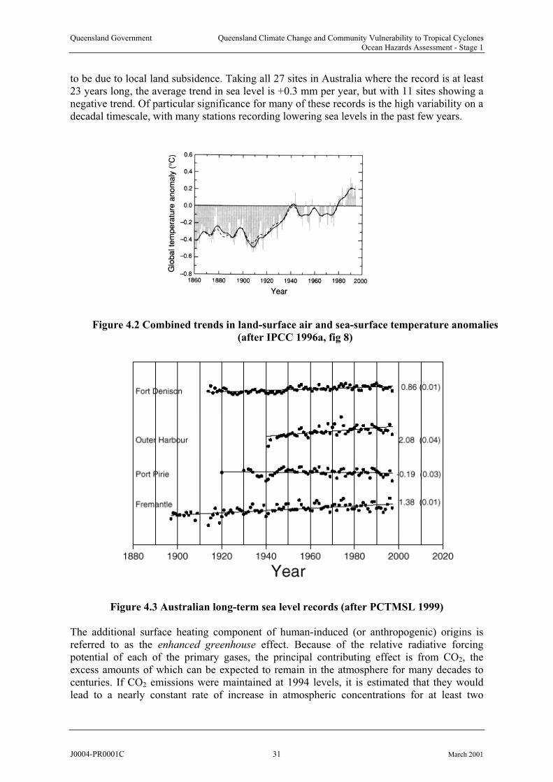
Queensland Government Queensland Climate Change and Community Vulnerability to Tropical CyclonesOcean Hazards Assessment - Stage 1
to be due to local land subsidence. Taking all 27 sites in Australia where the record is at least23 years long, the average trend in sea level is +0.3 mm per year, but with 11 sites showing a negative trend. Of particular significance for many of these records is the high variability on a decadal timescale, with many stations recording lowering sea levels in the past few years.
Figure 4.2 Combined trends in land-surface air and sea-surface temperature anomalies
(after IPCC 1996a, fig 8)
Figure 4.3 Australian long-term sea level records (after PCTMSL 1999)
The additional surface heating component of human-induced (or anthropogenic) origins is referred to as the enhanced greenhouse effect. Because of the relative radiative forcing potential of each of the primary gases, the principal contributing effect is from CO2, the excess amounts of which can be expected to remain in the atmosphere for many decades to centuries. If CO2 emissions were maintained at 1994 levels, it is estimated that they would lead to a nearly constant rate of increase in atmospheric concentrations for at least two
J0004-PR0001C 31 March 2001

Queensland Government Queensland Climate Change and Community Vulnerability to Tropical CyclonesOcean Hazards Assessment - Stage 1
centuries, reaching about 500 ppm (approaching twice the pre-industrial concentration of 280 ppm) by the end of the 21st century. This prediction is the basis of the commonly referred to
"2 CO2" scenario.
4.3 Latest Global Projections
Many of the existing numerical global climate models (GCMs) have had some success in reproducing broad climate behaviour but assume an equilibrium condition between theatmosphere and the ocean (the so-called slab model approach) which has limited their predictive capability. Meanwhile, the increasing realism of simulations of present and past climate by the more complex coupled atmosphere-ocean climate models has increased the confidence in their use for predicting climate change. Important uncertainties remain, but the IPCC believes these have been taken into account in the full range of projections of global mean temperature and sea level change. These are described by a series of modelled greenhouse gas emission scenarios, termed IS92a through to IS92f, which are predicated on world population estimates, economic growth and consequent energy usage patterns. The
range of temperature increases predicted by these scenarios varies between 1.5 C and 4.5 Cby the year 2100. Within each base scenario, model sensitivity testing has then beenundertaken using a range of model parameter assumptions.
The most-often quoted scenario is the IS92a, which is typically termed the "business as usual" outcome and implicitly assumes limited success of UNFCC plans. The IS92a scenario
produces an increase in mean global temperature of 2.5 C by the year 2100. The key projections of sea level increase by the year 2100 are presented in Table 4.1. These results also reflect sub-scenarios regarding sulfate aerosol emissions and are plotted in Figure 4.4 as a varying function of time.
Table 4.1 IS92a projected sea level increases to 2100
Sea level Rise IS92a
Scenario 1990 Aerosols Increasing
Aerosols
"low" 0.23 m 0.20 m
"mid-range" 0.55 m 0.49 m
"high" 0.96 m 0.86 m
The IS92a temperature estimate is approximately one third lower than the "best estimate" in 1990. This is due primarily to lower emission scenarios, the inclusion of the cooling effect of increasing aerosols, and improvements in the model treatments of the carbon cycle. It should be noted however that regional temperature changes might vary substantially from the global mean value. In addition, because of the thermal inertia of the oceans, temperature would continue to increase beyond 2100, even if concentrations of greenhouse gases were stabilised by that time.
The IS92a sea level rise estimate is approximately 25% lower than the "best estimate" in 1990 due to the lower temperature prediction, but also reflecting improvements in the climate and ice melt models. Likewise, sea level is expected to continue to rise beyond 2100 and even beyond the point of mean temperature stabilisation.
J0004-PR0001C 32 March 2001
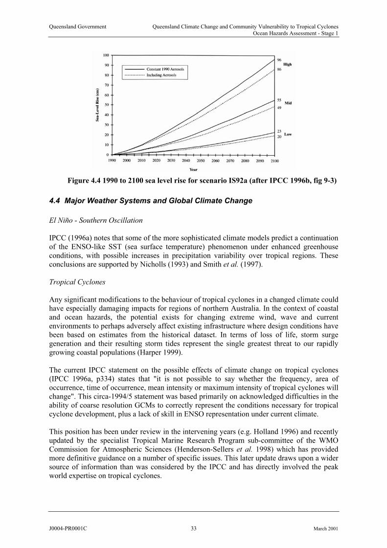
Queensland Government Queensland Climate Change and Community Vulnerability to Tropical CyclonesOcean Hazards Assessment - Stage 1
Figure 4.4 1990 to 2100 sea level rise for scenario IS92a (after IPCC 1996b, fig 9-3)
4.4 Major Weather Systems and Global Climate Change
El Niño - Southern Oscillation
IPCC (1996a) notes that some of the more sophisticated climate models predict a continuation of the ENSO-like SST (sea surface temperature) phenomenon under enhanced greenhouse conditions, with possible increases in precipitation variability over tropical regions. These conclusions are supported by Nicholls (1993) and Smith et al. (1997).
Tropical Cyclones
Any significant modifications to the behaviour of tropical cyclones in a changed climate could have especially damaging impacts for regions of northern Australia. In the context of coastaland ocean hazards, the potential exists for changing extreme wind, wave and currentenvironments to perhaps adversely affect existing infrastructure where design conditions have been based on estimates from the historical dataset. In terms of loss of life, storm surgegeneration and their resulting storm tides represent the single greatest threat to our rapidly growing coastal populations (Harper 1999).
The current IPCC statement on the possible effects of climate change on tropical cyclones(IPCC 1996a, p334) states that "it is not possible to say whether the frequency, area of occurrence, time of occurrence, mean intensity or maximum intensity of tropical cyclones willchange". This circa-1994/5 statement was based primarily on acknowledged difficulties in the ability of coarse resolution GCMs to correctly represent the conditions necessary for tropicalcyclone development, plus a lack of skill in ENSO representation under current climate.
This position has been under review in the intervening years (e.g. Holland 1996) and recentlyupdated by the specialist Tropical Marine Research Program sub-committee of the WMOCommission for Atmospheric Sciences (Henderson-Sellers et al. 1998) which has provided more definitive guidance on a number of specific issues. This later update draws upon a wider source of information than was considered by the IPCC and has directly involved the peak world expertise on tropical cyclones.
J0004-PR0001C 33 March 2001

Queensland Government Queensland Climate Change and Community Vulnerability to Tropical CyclonesOcean Hazards Assessment - Stage 1
The major conclusions of this later assessment are as follows:
Long-term reliable data on tropical cyclone intensity and frequency (which are largely limited to the North Atlantic and Western North Pacific regions) show substantial multi-decadal variability but there is no clear evidence of any long term trends in number,intensity or location.
Attempts to extend this record through analysis of geological and geomorphologicalrecords to establish a paleoclimate have so far not produced definitive results.
Recent thermodynamic modelling attempts to estimate the maximum potential intensity (MPI) of tropical cyclones in present climate has shown good agreement with observations (e.g. Holland 1997).
Application of MPI techniques to changed climate indicate the MPI of cyclones will remain the same or undergo a modest increase of up to 10 - 20% at the extreme end of the scale.
The broad geographic regions of cyclogenesis and therefore the regions affected by tropical cyclones are not expected to change significantly.
The region of cyclogenesis is unlikely to expand with the 26 C isotherm, i.e. the 28 Cisotherm is likely to become the new proxy reference temperature under present scenarios. The very modest available evidence points to an expectation of little or no change inglobal frequency.
Regional or local frequency of occurrence may however change substantially, in either direction, because of the dependence of cyclone genesis and track on other phenomena(e.g. ENSO) that are not yet predictable.
Mid-Latitude Systems
IPCC (1996a) notes that there is little agreement between climate models at present as to the likely changes in "storminess" which might occur in a warmer world. In the regional sense,some numerical studies (e.g. McInnes et al. 1992; Hopkins and Holland, 1997) haveattempted to explore possible changes to the behaviour of severe low-pressure systems such as "east coast lows".
In addition to the possible changes in frequency or severity of intense large-scale storms there may also be shifts in the mean synoptic patterns which could affect regional wind speeds and directions. This in turn could change the distribution of the wave-energy flux presently impacting the coastline. As explored by Gordon (1988), when combined with sea level rise, these more subtle changes may have a significant impact on the stability of coastal margins.Some potential evidence for changes in long term significant wave height is presented in Cox and Horton (1998).
4.5 Impact on the Oceans
Oceans occupy about 70% of the earth's surface. They provide an important component of the climate system, due to their role in controlling the distribution and transfer of heat and CO2
and in the transfer of freshwater back to the continents as precipitation. The oceans functionas regulators of the Earth's climate and sustain planetary biogeochemical cycles. They have significant capacity to store heat and are the largest reservoir of the two most important greenhouse gases - water vapour and carbon dioxide. About 60% of the Earth's radiative energy from the Sun is received by the oceans, 80% of that being absorbed within the top 10 m. Winds and waves mix down a seasonal surface layer of nearly uniform temperature,salinity and other properties which extends to tens of metres in the tropics and to several
J0004-PR0001C 34 March 2001
Queensland Government Queensland Climate Change and Community Vulnerability to Tropical CyclonesOcean Hazards Assessment - Stage 1
hundred metres in higher latitudes (the so-called upper thermocline). The permanent (lower) thermocline lies below the seasonal surface layer, down to about 1000 m. While wind-drivencirculation dominates the upper ocean mixing, manifesting as basin-scale gyres and intensive western boundary currents, the deeper ocean circulation is controlled by thermohaline processes (density currents). The lower thermocline and abyssal ocean represents nearly 90%of the volume of the oceans and most of this water is colder than 5°C. The oceans containabout 60 times more carbon than the atmosphere and variations in atmospheric carbon dioxide could result from even minor changes in the ocean's carbon cycling process, which is related to the ocean circulation. Conversely however, carbonate chemistry dictates that the ocean is not an especially efficient sink for human-induced increases in atmospheric carbon dioxide concentrations. Sea ice covers about 11% of the ocean and affects surface reflection of energy, salinity and ocean-atmosphere thermal exchange.
In the oceans, climate change will be accompanied by changes in temperature, circulation, sea level, ice coverage, wave climate and possibly extreme events:
Sea surface temperature (SST) increases are likely to be less than air temperatureincreases and to lag continental air temperature increases by as much as 10 years, before rising at a similar rate
Changes in SST gradients are expected to lead to a decrease in trade wind intensity, areduction in strength of upper ocean currents and a decrease in areas and intensity of upwelling
Due to a lack of basic understanding of the present interactions, it is still premature to project the behaviour of ENSO events for different climate changes
Available estimates of sea level changes are rather preliminary but will likely occur due toocean thermal expansion, changing volumes of polar and glacial ice sheets, dynamicalocean circulation effects, altered wind and weather patterns and differences in regional ocean density
Even the lower estimates of sea level rise are about 2 to 4 times the rate of sea level rise experienced in the last 100 years
Projected changes in climate should produce large reductions in the extent, thickness and duration of sea ice
Present numerical weather models are not yet capable of objectively estimating whether there is likely to be an increase in the frequency or intensity of severe tropical cyclones
Some corals are likely to be impacted through increased SST and possibly UVB exposure due to ozone depletion, leading to increased bleaching and a reduction in coral production
Increased loading of land-based pollutants is expected as a result of increasedprecipitation and atmospheric transport
4.6 Impact on Coastal Zones and Small Islands
It is estimated that 50 - 70% of the global human population (86% of Australians) live in the coastal zone, where important socioeconomic activities include resource exploitation (living and non-living), industry and commerce, infrastructure development, tourism, recreation and nature conservation. In most coastal nations, a considerable part of gross national product is derived from activities connected with the coastal zone. Many coastal problems presentlybeing experienced worldwide can be attributable to the unsustainable use and unrestricted development of coastal areas and resources. Climate change is likely to pose an additionalstress on these areas, with sea level rise and possible changes in the frequency and intensity of extreme events being of prime concern. In addition to the physical changes that are possible,
J0004-PR0001C 35 March 2001
Queensland Government Queensland Climate Change and Community Vulnerability to Tropical CyclonesOcean Hazards Assessment - Stage 1
climate change has the potential to significantly affect coastal biological diversity through alteration of habitat.
The following are the major aspects of concern to the coastal zone and small islands:
Any changes in sea level are expected to vary from the global mean over regional and local scales due to (1) vertical land movement e.g. subsidence, upheaval and (2) dynamicalocean effects due to circulation patterns, wind and pressure distributions and density differences. These are effects, which already dictate global variation in mean sea level, but the possible changes caused by a warming climate are unknown at this stage.
A 2 C change in mean SST would mean that values presently considered anomalous (of the order of peak ENSO fluctuations) could well be normal occurrences, with resultantlong-term stress on natural ecosystems that are unable to effectively adapt.
Increased precipitation is expected throughout the year in high-latitudes and during the winter in mid-latitudes, possibly increasing coastal deposition rates. Some increase inAsian monsoon rainfall is also predicted.
Changes in storm patterns or general shifts in mean weather conditions (windiness, wave energy and direction) are not able to be reliably estimated at this time but could have significant long term impacts on coastal stability and alignments.
Any potential increase in the frequency, magnitude or extent of very severe weather systems such as tropical cyclones would severely impact coastal regions, with the potential for enormous loss of life and devastating impacts on coastal ecosystems and morphology.Fortunately, the present predictions show a low likelihood of significant changes occurring to these systems.
The possibility of sea level rise alone forms a basis for considering a number of major impactsfor the coastal zone, such as:
inundation and displacement of wetlands and lowlands
eroded shorelines
increased coastal flooding by storms
salinity intrusion of estuaries and aquifers
altered tidal ranges, prisms and circulation in estuarine systems
changed sedimentation patterns
decreased light penetration
Coral reefs and reef islands appear especially susceptible to climate change and associated sea level rise. The erosion of the coastline, inundation and flooding of low lying areas andseawater intrusion into groundwater lenses will all act to reduce the habitability of such regions. However, individual responses are likely to vary greatly because of sedimentavailability, available freeboard, aquifer characteristics and general resilience of the naturalsystems.
Normal rates of coral growth are thought sufficient to keep pace with projected rates of sea level rise and in some situations may even benefit from an increased water level. It is also conjectured that coral biota may be able to adjust to the projected rate of water temperatureincreases without succumbing to bleaching effects. However, reduced resilience caused byUVB increases may restrict this ability. Additionally, many coral reef areas are alreadythought to be adversely affected by rainfall and urban runoff, which may increase in someareas under a changed climate.
J0004-PR0001C 36 March 2001

Queensland Government Queensland Climate Change and Community Vulnerability to Tropical CyclonesOcean Hazards Assessment - Stage 1
4.7 Australian Regional Predictions and Impacts
The most recent regional climate change projections for Australia are presented in CSIRO (1996). Potential broad-scale impacts of these projections form the basis of a national vulnerability assessment by Basher and Pittock (1998) in IPCC (1998). CSIRO scenarios for
Australia indicate possible temperature increases of 0.3 C to 1.4 C by 2030, approximatelydoubling by 2070. Total rainfall trends vary across the continent and have seasonal aspects but with changes up to 10% in magnitude relative to present norms, the overall tendency being for decreases. In spite of this, an increase in intensity of heavy rainfall events ispredicted. There are no specific projections of regional sea level rise in addition to IPCC (1996a) nor are there any trends for tropical cyclone effects which are at variance with Hendersen-Sellers et al. (1998), e.g. Walsh and Pittock (1998), McInnes et al. (2000), Walshand Ryan (2000). These predictions must still be viewed within the context that, relative to their assessed global performance, existing climate models are considered to have reduced skill at subcontinental scales. CSIRO (1996) also relies on a combination of slab model and coupled models because of some doubts about the reliability of scenarios from the coupledmodels versus latitudinal warming gradients and trends in summer rainfall across Australia.
A wide range of vulnerability and impact studies have been undertaken for various areas ofAustralia and the South Pacific over the past ten years. Some early studies (e.g. Pearman et
al. 1988) which predate IPCC (1996a) must be reinterpreted in terms of the revised climateprojections, but otherwise still contain useful guidance on some specific regional issues. Themajority of studies have been undertaken by and for State and Commonwealth authorities through research grants under the Australian Greenhouse Office and also with specific State funding, e.g. Bouma et al. (1996). A number of regional climate change scenarios are also available, which are essentially the same as the overall Australian view but with localisedcommentary, e.g. CSIRO (1998), specific climate change scenarios for northern Australia. In regard to specific coastal vulnerability issues, Waterman (1996) summarises a number of studies undertaken for the Commonwealth Department of Environment, Sport and Territoriesfrom 1994 to 1996, although in the Queensland context this is limited to DEH (1996) for Mackay. The earliest storm tide study that included a Greenhouse assessment is due to Hardy et al. (1987), while McInnes et al. (2000) provides a more recent assessment for Cairns. Henderson-Sellers (1996) provides an overview of issues and possible adaptive options confronting Oceania in general.
4.8 Conclusions and Recommendations
NCCOE (2001) concurs that the weight of scientific opinion suggests that baseline changes to climate may occur within the design life of much of our coastal and ocean communityinfrastructure. Consequently, consideration of the possible impacts of climate change should be included in the design processes and in long term planning. The overall response to "greenhouse" though should be seen as an expansion of current methodologies where natural variability of climate still dominates considerations of risk. In spite of the enormous and growing body of scientific literature and knowledge of global warming, there are unlikely tobe definite predictions of its effects or panaceas for its possible impacts. It is therefore essential that good judgement be also exercised at all times.
In regard to the impacts of climate change on storm tide risks caused by tropical cyclones, it
is recommended that consideration should be given to:
J0004-PR0001C 37 March 2001
Queensland Government Queensland Climate Change and Community Vulnerability to Tropical CyclonesOcean Hazards Assessment - Stage 1
1. Mean sea level rise scenarios over time (e.g. 0.49 m by 2100)
2. Some increase (e.g. 10% to 20%) in the maximum potential intensity of individual
cyclones (MPIs)
It is important to note the latter recommendation should be introduced as a lowering of the MPI physical limit rather than an across-the-board lowering of central pressures.
It is not considered essential to allow for any specific change in the frequency of occurrenceor geographical limit of tropical cyclone activity in the Queensland region since there is insufficient analysis upon which to draw a conclusion.
Until such analyses prove otherwise, it is recommended that model sensitivity to the frequency
of occurrence or geographical limit of tropical cyclones should be tested as part of a
comprehensive hazard assessment methodology, i.e. inclusion of a nominal 10% variation.
4.9 References
Basher R.E. and Pittock A.B. (1998) Australasia. In: The regional impacts of climate change - an assessment of vulnerability. [IPCC, 1998], Cambridge University Press, ISBN 0-521-634555, 106-148.
Bouma W.J, Pearman G.I. and Manning M.R. (eds.) (1996) Greenhouse: coping with climatechange, CSIRO Publishing, Collingwood, Vic.
Cox R.J. and Horton, P.R. (1998) Managing climate change in the coastal zone. Proc. Australian Global Warming Conf..
CSIRO (1996) Climate change scenarios for the Australian region. Climate Impact Group, CSIRO Div Atmospheric Research, Melb, Nov, 8pp.
CSIRO (1998) Climate change under enhanced greenhouse conditions in northern Australia - Final report 1994-1997. CSIRO Div of Atmospheric Research, Jan, 49pp, ISBN 0643060170.
DEH (1996) Methodology for climate change vulnerability assessment of Mackay coast. Coastal Resource Assessment Section, Coastal management branch. Prep by Qld Dept of Environment and Heritage for the Commonwealth Dept of Environment, Sport and
Territories.
Dept of the Environment (1997) Climate change: Australia's second national report under the United Nations framework on climate change. Commonwealth of Australia, Nov, ISBN 0642194610, 125 pp.
Gordon, A.D. (1988) A tentative but tantalizing link between sea-level rise and coastal recession in New South Wales,. In Greenhouse: Planning for Climate Change [Pearman, G.I. (ed.)], CSIRO Publishing, Collingwood, VIC, 121-134.
J0004-PR0001C 38 March 2001

Queensland Government Queensland Climate Change and Community Vulnerability to Tropical CyclonesOcean Hazards Assessment - Stage 1
Harper B.A. (1999) Storm tide threat in Queensland: History, prediction and relative risks. Conservation Technical Report No. 10, Dept of Environment and Heritage, Jan, ISSN 1037-4701.
Henderson-Sellers A., Zhang H., Bertz G., Emanuel K., Gray W., Landsea C., Holland G., Lighthill J., Shieh S-L.,Webster P. and McGuffie K. (1998) Tropical cyclones and global climate change: a post-IPCC assessment. Bull. of the Amer Met. Soc., 79, 1, January, 19-38.
Henderson-Sellers A. (1996) Adaptation to climate change: its future role in Oceania. In: Greenhouse: Coping with Climate Change [Bouma, W.J, Pearman, G.I. and Manning M.R. (eds.)]. CSIRO Publishing, Collingwood, VIC, 349-376.
Holland G.J. (1996) Tropical cyclone intensity and intensity change: A review and outlook. ONR Symposium on Tropical Cyclones: State of Understanding and Future Directions, Bureau of Meteorology, Melb, Dec 9-13.
Holland G.J. (1997) The maximum potential intensity of tropical cyclones. J. Atmos. Sci., Vol 54, Nov, 2519-2541.
Hopkins L.C. and Holland G.J. (1997) Australian heavy-rain days and associated east coast cyclones: 1958-92. Journal of Climate, 10, 621-635.
IPCC (1996a) Climate change 1995 - the science of climate change. Contribution of working group I to the second assessment report of the intergovernmental panel on climate change, Cambridge University Press, ISBN 0 521 56436 0, 572pp.
IPCC (1996b) Climate change 1995 - impacts, adaptations and mitigation of climate change: scientific-technical analyses. Contribution of working group II to the second assessmentreport of the intergovernmental panel on climate change, Cambridge University Press, ISBN 0 521 56437 9, 879pp.
IPCC (1996c) Climate change 1995 - economic and social dimensions of climate change. Contribution of working group III to the second assessment report of the intergovernmentalpanel on climate change, Cambridge University Press, ISBN 0 521 568544.
IPCC (1998) The regional impacts of climate change - an assessment of vulnerability. A special report of IPCC Working Group II, Cambridge University Press, ISBN 0-521-634555.
McInnes K. L., Leslie L. M. and McBride J. L. (1992) Numerical simulation of cut-off lowson the Australian east coast: sensitivity to sea-surface temperature. J. Climate, 12, 783-795.
NCCOE (2001) Guidelines for responding to the effects of climate change in coastal and ocean engineering. National Committee on Coastal and Ocean Engineering, IEAust. (inpreparation)
Nicholls N. (ed.) (1993) Climate change and El Niño southern oscillation, BMRC Res. Rep No 36, Bureau of Meteorology, Melbourne, 31pp.
PCTMSL (1999) Permanent committee on tides and mean sea level - circular 43. Defence
Publishing Service, Department of Defence, May, 8pp.
J0004-PR0001C 39 March 2001

Queensland Government Queensland Climate Change and Community Vulnerability to Tropical CyclonesOcean Hazards Assessment - Stage 1
Pearman G.I. (ed.) (1988) Greenhouse: planning for climate change. CSIRO Publishing,Collingwood, VIC, 752pp, ISBN 0 643 04863 4.
Smith I.N., Dix M. and Allan R.J. (1997) The effect of greenhouse SSTs on ENSO simulations with an AGCM. Journal of Climate, 10, 342-352.
Walsh K. and Pittock A.B. (1998) Potential changes in tropical storms, hurricanes, andextreme rainfall events as a result of climate change. Climatic Change, 39, 199-213.
Walsh K.J.E. and Ryan B.F. (2000) Tropical cyclone intensity increase near Australia as aresult of climate change. Jnl. Climate (to appear).
Waterman P. (ed.) (1996) Australian coastal vulnerability assessment project report. Dept of
the Environment Sport and Territories, Australian Government, Canberra, 2 Vols / CDROM.
J0004-PR0001C 40 March 2001

Queensland Government Queensland Climate Change and Community Vulnerability to Tropical CyclonesOcean Hazards Assessment - Stage 1
5. Tropical Cyclone Wind and Pressure Modelling
5.1 The Need for Simplified Models
This section introduces the need for simplified parametric models for hazard studies andpresents some of the technical bases for a typical model in popular usage. An example wind field pattern is also presented for reference purposes. Areas where there are opportunities for model results to significantly differ are highlighted in the discussion. The development here is drawn from WMO (1988) and also the subsequent work by Harper and Holland (1998), a state-of-the-art review commissioned by the Risk Prediction Initiative, Bermuda.
The tropical cyclone (hurricane or typhoon) is an extremely complex meteorologicalphenomenon but from a descriptive viewpoint is still amenable to analytical simplification,provided that the essential time and space scales of motion are preserved. This descriptivereconstruction process is separate from the very difficult questions of prediction of intensification and movement of tropical cyclones that beset forecasters. These questionscontinue to be the subject of intensive research into the basic physics and dynamic interaction of the storm with its environment, both atmosphere, ocean and land, throughout its life. Somevery complex numerical models of tropical cyclone behaviour are now available whichattempt to represent the full 3-dimensional interactions of the storm (e.g. Kurihara et al. 1995; Wang and Holland 1996; Kepert 2000; Kepert and Wang 2000). As these models continue to be developed and computer power increases it is likely that these deterministic models will, in association with better environmental data sets and improved physical parameterisations,continue to gain accuracy and skill. However, such models are presently too cumbersome and computationally expensive to be applied to the types of studies required for long-term risk assessment. This is because a large number of storm scenarios need to be considered across wide areas to develop the statistical basis required for risk estimation. In addition, deterministic models will eventually reach a limit of representation where stochastic processesbegin to dominate the prediction of storm behaviour. It is likely that these stochastic elementsremain very important in individual storm scenarios and the appropriate statisticalrepresentation of their occurrence may become the single most important factor in the estimation of insured losses from tropical cyclones. Techniques utilising simplifiedparametric models already have the capacity to incorporate this type of stochastic variabilityinto risk assessments, albeit at a lower level of representation.
Since we are interested in impacts of tropical cyclones at the surface (land or ocean), the emphasis is on the representation of the near-surface (horizontal) wind and pressure field as it evolves with time. Developments over several years have resulted in such models furnishing simplified descriptions of the essential wind (and pressure) profiles that provide spatial andtemporal surface forcing for use in a variety of complex engineering, numerical modellingand risk assessment studies such as
offshore facilities wind, wave, continental shelf current and storm surge design criteria
onshore infrastructure design (eg ports, public housing, wind sensitive structures)
public evacuation and disaster planning (wind and storm surge)
insurance risk assessment
J0004-PR0001C 41 March 2001
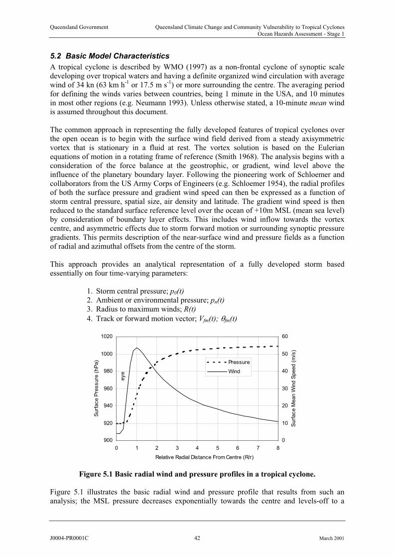
Queensland Government Queensland Climate Change and Community Vulnerability to Tropical CyclonesOcean Hazards Assessment - Stage 1
5.2 Basic Model Characteristics
A tropical cyclone is described by WMO (1997) as a non-frontal cyclone of synoptic scale developing over tropical waters and having a definite organized wind circulation with average wind of 34 kn (63 km h-1 or 17.5 m s-1) or more surrounding the centre. The averaging period for defining the winds varies between countries, being 1 minute in the USA, and 10 minutesin most other regions (e.g. Neumann 1993). Unless otherwise stated, a 10-minute mean wind is assumed throughout this document.
The common approach in representing the fully developed features of tropical cyclones over the open ocean is to begin with the surface wind field derived from a steady axisymmetricvortex that is stationary in a fluid at rest. The vortex solution is based on the Eulerian equations of motion in a rotating frame of reference (Smith 1968). The analysis begins with a consideration of the force balance at the geostrophic, or gradient, wind level above theinfluence of the planetary boundary layer. Following the pioneering work of Schloemer and collaborators from the US Army Corps of Engineers (e.g. Schloemer 1954), the radial profiles of both the surface pressure and gradient wind speed can then be expressed as a function of storm central pressure, spatial size, air density and latitude. The gradient wind speed is thenreduced to the standard surface reference level over the ocean of +10m MSL (mean sea level) by consideration of boundary layer effects. This includes wind inflow towards the vortex centre, and asymmetric effects due to storm forward motion or surrounding synoptic pressure gradients. This permits description of the near-surface wind and pressure fields as a function of radial and azimuthal offsets from the centre of the storm.
This approach provides an analytical representation of a fully developed storm based essentially on four time-varying parameters:
1. Storm central pressure; p0(t)
2. Ambient or environmental pressure; pn(t)
3. Radius to maximum winds; R(t)
4. Track or forward motion vector; Vfm(t); fm(t)
900
920
940
960
980
1000
1020
0 1 2 3 4 5 6 7 8
Relative Radial Distance From Centre (R/r)
Surf
ace P
ressure
(hP
a)
0
10
20
30
40
50
60
Surf
ace M
ean W
ind S
peed (
m/s
)
Pressure
Wind
eye
Figure 5.1 Basic radial wind and pressure profiles in a tropical cyclone.
Figure 5.1 illustrates the basic radial wind and pressure profile that results from such an analysis; the MSL pressure decreases exponentially towards the centre and levels-off to a
J0004-PR0001C 42 March 2001

Queensland Government Queensland Climate Change and Community Vulnerability to Tropical CyclonesOcean Hazards Assessment - Stage 1
relatively flat region of lowest pressure inside the cyclone “eye” (920 hPa in this example).The winds initially increase exponentially towards the centre, driven by the increasing pressure gradient and reach a maximum at the so-called radius of maximum winds, before rapidly dropping to calm in the centre. While many real storms may not always exhibit such symmetry and form throughout their full life cycle, this basic model does appear to well represent the essential force balance and spatial variability of the tropical cyclone. In moresophisticated models additional parameters are often added, as detailed in the followingsections.
For the purpose of illustration, the Holland (1980) model development is followed here, but replacing the Holland A parameter by its equality R
B. The model relies on the primaryassumption of a radially symmetric pressure field derived from Schloemer (1954) but with a modified rectangular hyperbola to give the pressure p at any radius (r) from the centre as:
p(r) = p0 + (pn - p0) exp (-R/r)B (5.1)
Here an additional fifth parameter "B" is introduced to add to the basic set of descriptivestorm parameters previously listed. Holland recognised that the basic Schloemer profile lacked sufficient dynamic range to match many steep storm pressure profiles such as Tracy
and subsequently added the B parameter - the so-called profile “peakedness”. When B is set tothe lower limit of 1, the profile is equivalent to the classic Schloemer formulation and Holland nominally limited its range based on simple physical arguments to lie within 1 < B < 2.5.
The gradient level winds are then derived by considering the balance between the centrifugal and Coriolis forces acting outwards and the pressure force acting inwards, leading to thegradient wind balance equation:
Vg2(r)/r + f Vg = 1/ a dp(r)/dr (5.2)
where Vg = gradient level wind
a = air density
f = Coriolis parameter (2 sin )
and the pressure gradient from differentiation of (5.1) is given by:
dp(r)/dr = (pn - p0) (B/r) (R/r)B exp (-R/r)
B (5.3)
which substitutes into (5.2) to yield the gradient wind at any radius as: ________________________________
Vg (r) = ( (pn - p0) B/ a (R/r)B exp (-R/r)
B + r
2f2/4 ) - rf/2 (5.4)
At r = R the maximum gradient wind speed is given by: _______________________
Vgmax = ( (pn - p0) B / (e a) + R2f2/4 ) - rf/2 (5.5)
but since the Coriolis terms are normally negligible at r = R, this reduces effectively to: _______________
Vgmax = ( (pn - p0) B /(e a) (5.6)
J0004-PR0001C 43 March 2001

Queensland Government Queensland Climate Change and Community Vulnerability to Tropical CyclonesOcean Hazards Assessment - Stage 1
where it can be seen that for the Holland model, the pressure differential is further modulated
by B over the original Schloemer estimate for Vgmax, thus providing a further dynamic range up to a factor of 1.6. Based on the climatological work by Atkinson and Holliday (1977) and Dvorak (1975), Holland also suggested “standard” B values might be inferred of the form:
B = 2 - (p0- 900)/160 (5.7)
making B a direct function of storm intensity. To allow for possible climatological variabilityin such a trend this can also be generalised to a “family” of like curves which might apply to aspecific storm’s lifetime, e.g.
B = B0 - p0(t)/160 (5.8)
where B0 is the intercept value of the trend.
A potentially important component missing from both the Holland and other wind profile formulations, is the variation of air density with pressure towards the cyclone centre. Introducing this variation changes the wind peakedness significantly and might lead to moreeasily defined values of B.
5.3 Boundary Layer Representation
Equation (5.4) provides a radially symmetric profile of estimated gradient level winds which must be transferred to be representative at the surface. Traditionally, this adjustment to the surface (+10m) has been based on similarity theory and the logarithmic deficit law approach, whereby the near-surface boundary layer profile at any height z is a function of the surface roughness z0 and the reference wind speed. This is clearly an oversimplification of thecomplex dynamics of the tropical cyclone boundary layer, many aspects of which are stillemerging (e.g. Kepert and Wang 2000). However, in the absence of better information this approach has permitted reasonable calibration against a range of measured results undertropical cyclone conditions. This assumption results in the mean near-surface wind Vm, under assumed neutral stability conditions, being estimated by an equation of the form:
Vm = Km Vg (5.9)
where Km = ln(10/z0)/ln(zg/z0) (5.10)
and zg = gradient wind height Vg (z=zg)
Over the open ocean, the surface roughness is dynamically a function of wave growth with time, while over land it varies spatially according to the natural and built environment. Open ocean roughness values are generally accepted as ultimately reaching levels similar to lightlytimbered savanna.
Application of this theoretical approach is strictly limited to stationary wind conditions where the peak gust is related to a mean wind reference by a Gaussian distribution function. Accordingly, a representative mean wind-averaging period of 10 minutes is often used to establish the mean profile and then gust factors are re-applied to suit various applications such as 2 or 3 sec gusts. In this context Vm is to be considered as a 10 minute averaged windsample. A basic limitation of this theory is that convective storm elements, especially within
J0004-PR0001C 44 March 2001

Queensland Government Queensland Climate Change and Community Vulnerability to Tropical CyclonesOcean Hazards Assessment - Stage 1
rainbands, are thought capable of allowing gradient winds to penetrate to the surface withoutthe assumed vertical mixing processes occurring. Also, microburst and vortex breakdown components can simply add horizontal wind at the surface as localised transient features. These essentially convective elements are becoming recognised as at least partially responsible for relatively high gust factors often being reported in landfalling tropical cyclones (Holland and Black pers. comm. 1997).
A variety of values for Km exist in the literature and some of the early choices are mentionedlater, the differences being complicated by the often unstated choice of averaging period for the surface wind. For example, Powell (1980) proposed 0.8 but his later observational studies (e.g. Powell and Black 1989; Powell et. al. 1991; 1998) have reported variability over the range 0.7 to 0.9, which has normally been attributed to vertical stability differences. As an order of magnitude, it is believed that Km can be considered as approximately 0.7 over the ocean which, when combined with a peak gust factor of order 1.4, typically delivers 2 to 3 sec gusts basically equivalent to the gradient speed. Microbursts and other transient featuresmight further cause super-gradient winds to develop locally for short periods. Kepert (2000) also introduces the possibility that Km may in fact be azimuthally varying due to the complexvertical structure of the boundary layer. The potentially arbitrary choice of Km and associatedwind averaging periods is typically a major source of variation between “similar” parametricmodels and can have significant impact on predicted surface stress magnitudes anddistributions.
In addition to the scalar reduction in wind speed, surface friction and continuity demand that the wind must flow inward across the isobars. The angle of inflow is taken to be
approximately 25 in the outer region (e.g. Shea and Gray 1973), but reduces to zero near the radius of maximum winds. For example, Sobey et al. (1977) adopted the following, based on US Weather Bureau (1968):
(10 (r/R) 0 r < R (5.11)
= (10 + 75 (r/R-1) R r < 1.2 R
(25 r 1.2 R
5.4 Forward Motion Asymmetry
Tropical cyclone motion produces complex changes to the surface wind field that are intrinsically related to the 3-dimensional structure of the storm, the underlying surface conditions, and the atmospheric environment within which the cyclone is embedded. Parametric models to date have sought to reproduce only the first-order effects of the observed forward motion on the surface windfield. In some cases, the forward motion vector has been added to the wind field at the gradient level, then reduced to the surface by thestandard techniques described above. The preference here though is that the forward speed is directly added at the surface since it is a manifestation of movement at the surface. This provides a left-right asymmetry, with the maximum winds to the left (right) when looking in the direction of motion of the cyclone in the Southern (Northern) Hemisphere. The actual location of the region of maximum surface winds in individual storms can occur almostanywhere (Jelesnianski and Holland 1993; Kepert 2000).
This asymmetry is thus achieved by various models such that some proportion of the forward
speed fm (typically 0.5 or 1) is added at the surface along an assumed line of maximum winds
max (measured upwind relative to the cyclone movement direction) and then azimuthally adjusted about the storm, e.g.
J0004-PR0001C 45 March 2001

Queensland Government Queensland Climate Change and Community Vulnerability to Tropical CyclonesOcean Hazards Assessment - Stage 1
Vm(r, ) = Km Vg(r) + fm Vfm cos( max - ) (5.12)
and when = max and r = R, the maximum surface wind speed in the storm is:
Vmmax = Km Vgmax + fm Vfm (5.13)
This is perhaps the least satisfactory aspect of the current empirical approaches to modelling
the cyclone surface wind field. Values chosen for max have varied, with early estimates being 115º (rear left) based inferred from Graham and Nunn (1959) with later values being around 65º (front left) consistent with, for example, Shapiro (1983) and now Kepert (2000).
5.5 A Typical Parametric Wind Field Representation
Based on the foregoing description, Figure 5.2 presents an example parametric mean wind field of a fully developed tropical cyclone over the ocean, together with a crossection of meanwind and pressure normal to the direction of movement. The storm is presented as a Southern Hemisphere example moving south. The full set of parameters used is listed in Table 5.1 below.
Table 5.1 Example Storm Parameter Set
Parameter Symbol Value Units
Latitude -20
Central Pressure p0 920 hPa
Ambient Pressure pn 1010 hPa
Radius to Max Wind R 30 km
Forward Speed Vfm 4 m s-1
Bearing fm 180
Peakedness B 1.5 -
Asymmetry Factor fm 1.0 -
Line of Max Wind max 65
Air Density a 1.15 kg m-3
B/L Coefficient Km 0.67 -
The Vmmax resulting from this combination at r = R along the line of maximum winds is 53.6
m s-1 located in the front left stormwise quadrant (65 left or upwind of the forward motionvector).
J0004-PR0001C 46 March 2001
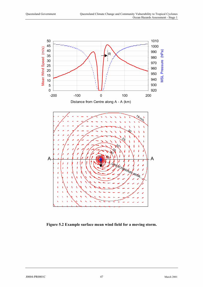
Queensland Government Queensland Climate Change and Community Vulnerability to Tropical CyclonesOcean Hazards Assessment - Stage 1
20
30
45
40
35
25
15 m/s
Line of maximumwinds
A A
0
5
10
15
20
25
30
35
40
45
50
-200 -100 0 100 200
Distance from Centre along A - A (km)
920
930
940
950
960
970
980
990
1000
1010
MS
L P
ressure
(h
Pa)
R
Mean W
ind S
peed
(m/s
)
Figure 5.2 Example surface mean wind field for a moving storm.
J0004-PR0001C 47 March 2001

Queensland Government Queensland Climate Change and Community Vulnerability to Tropical CyclonesOcean Hazards Assessment - Stage 1
5.6 Historical Development of Windfield Models
Some of the early development presented here follows essentially the work by Lovell (1990) who identified 24 separate parametric wind field model descriptions that had been published up until the late 1980s. His conclusion was that almost all popular formulations were essentially variations on those first developed by either the US Weather Bureau and the USArmy Corps of Engineers in the 1950s (firstly by the Hydrometeorological Section and then by the joint National Hurricane Research Program (NHRP)) or by Holland (1980). The apparent proliferation of models in various forms over the years has resulted mainly because many authors failed to adequately acknowledge the original sources for the parametricformulations or inadvertently disguised the pedigrees by the introduction of simplifyingconstants, non-dimensionalising of equations and the like.
5.6.1 Earliest Studies
Takahashi (1939, 1952) and Hughes (1952) were instrumental in proposing some early empirical methods while perhaps the earliest attempt at describing the full wind field in aparametric manner dates to Depperman (1947) in a study of Philippine typhoons. This is the so-called Rankine-combined or modified potential vortex, where the radial wind field at gradient height is given by:
Vg = Vgmax (r/R) r < R (5.14a)
Vg = Vgmax (r/R)-x
r > R (5.14b)
The shape parameter x allows the outer wind profile beyond R to be modified to fit available data. For physical reasons 0 < x < 1 with a practical range 0.3 < x < 0.8 and a typical application value of 0.5. The Rankine vortex model is mentioned for completeness rather than practical application. This is because practitioners find it often produces a profile that generally under or over shoots measured winds.
5.6.2 US Army Corps of Engineers Impetus
A number of specific studies were undertaken by the US Weather Bureau on behalf of the US Army Corps of Engineers over the period 1954 through to the early 1960s, which were aimedat producing objective techniques for estimating hurricane intensities.
The first study was by Schloemer (1954), who developed a model pressure profile to plan levee heights for storm surge impacts on Lake Okeechobee in Florida. Although the profile was based on limited pressure data from only nine storms it appears to have captured the essential broad-scale form of the radial pressure relationship. His exponential pressure profilewas based on the general principle that:
(p-p0) / (pn-p0) = f(r) (5.15)
Schloemer applied the exponential pressure profile to the cyclostrophic wind balance equation to provide a radial wind profile and derived a value for Vgmax. He also proposed a value for Km and the surface inflow angle. His work was significant in being the first to specify a continuous radial wind profile in pressure balance and to recognise the significance of the
J0004-PR0001C 48 March 2001
Queensland Government Queensland Climate Change and Community Vulnerability to Tropical CyclonesOcean Hazards Assessment - Stage 1
environmental pressure, an R scale and the surface boundary layer effects. Fletcher (1955) provided further dissemination of Schloemer’s work for general application in estimatingmaximum surface winds.
Myers (1954) extended Schloemer’s work in applying it to a statistical analysis to establishdesign criteria. He replaced the cyclostrophic balance by the gradient balance (i.e. including Coriolis effects) to obtain better data matches at outer radii. He also further examined the Km
issue and considered the difference in roughness regimes and transition lengths between onshore and offshore winds. Out of this work came the recommendation to apply the (muchquoted to three significant figures) Km of 0.865 for transfer of gradient winds to off-water Vm.This was predicated on the assumption that the peak 3 second gust approximately equalled thegradient wind V. Myers also examined the possible relationship between R and stormintensity, noting that the highest wind speeds in very intense hurricanes tended to becomemore spatially limited.
This work continued with the National Hurricane Research Project (NHRP) in 1955 and Graham and Nunn (1959) developed the so-called Standard Project Hurricane (SPH) indices for seven differing geographic zones along the East and Gulf coasts of the US. These indices were based on applying Myer’s equations to a database of storms over the period 1900 to
1956. They also introduced forward motion asymmetry allowances using a fm of 0.5 and
selected max as -115 based on observational studies. Finally, they made recommendations in regard to transition zones and, although generally applying the Myer’s Km of 0.865, were swayed by one set of measurements to allow 0.885 for one of the Gulf regions. Their recommendations were published as a series of nomograms for forecaster use, the radial windprofiles not exactly following the theoretical curve but allowing for empirical shape variations on a regional basis.
Graham and Hudson (1960) continued the work by looking at further cases in detail, including extra-tropical storms, and adjudged Schloemer’s pressure profile considerably in error in the outer portions of the profiles. They were the first to consider introducing the B
exponent to objectively address this, Graham and Nunn already having empirically adjusted the regional outer wind profiles to suit. Ironically, the B parameter here was proposed for reasons opposite to that later to be considered by Holland in regard to the peak portion of the profile.
Over this period a number of theoretical and observational studies of hurricane wind fields contributed to increasing knowledge. These included Colon (1961), Miller (1958,1962), Kraft(1961), Rhiel (1962) and Rosenthal (1961,1962). Further updates of the NHRP followed overtime with US Weather Bureau (1968) first introducing the probable maximum hurricane
(PMH), with later updates by Schwerdt (1972) and finally Schwerdt et al. (1979).
5.6.3 Growth of Applications
Subsequent works then concentrated on the application of these techniques for planning and warning purposes, especially in regard to storm surge prediction (Harris 1958; Harris and Jelesnianski 1964; Marinas and Woodward 1968) and the burgeoning Gulf of Mexico offshore oil and gas developments.
Jelesnianski (1965,1966) adopted the Schloemer pressure profile for incorporation into his numerical hydrodynamic model for storm surge but chose not to apply the balanced wind
J0004-PR0001C 49 March 2001
Queensland Government Queensland Climate Change and Community Vulnerability to Tropical CyclonesOcean Hazards Assessment - Stage 1
profile. This may have been more for computational convenience at the time, his formulabeing:
Vm(r) = (2 Vmmax + Vfm) R r / (R2+ r
2) (5.16)
This later led to the development of the US Weather Service SPLASH storm surge prediction model (Jelesnianski and Taylor 1973) and the SLOSH model (Jelesnianski et al. 1992).
Many other workers continued to explore variations on the NHRP theme, increasinglytargeted now at computer application of the SPH nomograms, and to try to accommodate the additional dynamic range needed from the Schloemer profile. Collins and Viehman (1971)presented a re-examination of unpublished NHRP data (Goodyear and Nunn 1965) correlating R vs V/Vmmax, ostensibly to provide a “simplified” model but arguably not succeeding.Patterson (1972) provided an (ill-conditioned polynomial) variant for use in early numericalwave models, in conjunction with work by Wilson (1961,1966). Bretschneider (1972) had considerable impact in ocean engineering application but merely provided a non-dimensional
form of Graham and Nunn’s work with an added climatological variation based on a. His nomogram wind field was widely adopted for coastal and offshore engineering design through incorporation into various editions of the US Army Corps of Engineers design manual issued by CERC (1984). This has now been supplanted by the Holland (1980) model in the new CERC design manual (not yet released).
Cardone et al. (1976) introduced the next most dramatic change in approach to the problem by applying a numerical boundary layer solution targeted at wave prediction improvements.Their model still contained aspects of the Schloemer recommendations and utilised a form of R in specifying the symmetric vortex pressure profile. Their resulting model, used extensively in offshore design criteria work, is essentially numerical rather than parametric, based onearlier work by Chow (1971) and Cardone (1969).
Other oceanographers and ocean engineers adopted a number of different model approachesover this period. Russell (1971) published a further variant; Overland (1977) provided a review of methods; Ross (1979) modified Patterson (1972) in conjunction with the JONSWAP wave experiment (Hasselmann et al. 1973); Forristall (1980) adopted Patterson (1972), attributing it to Wilson (1961); Wang (1987) adopted Patterson (1972) but attributed it to Forristall (1980).
Wind engineers at this time also took advantage of the increasing availability of parametricmodels and applied them to the estimation of design wind speeds for construction. Typical applications of the Schloemer-Myers form included Martin (1974), Simiu et al. (1976),Gomes and Vickery (1976) and Batts et al. (1980).
In developing the first numerical storm surge model for Australian conditions, Sobey et
al.(1977) and Harper (1980), adopted the Schloemer pressure profile and Vmmax estimates.They also fitted a separate B parameter to match the range of Graham and Nunn (1959) empirical wind profiles, the outer region equation being:
V(r) = Vgmax exp( B(1-r/R) ) r > R (5.17a)
where B = 0.0025R + 0.05 for R in km. (5.17b)
J0004-PR0001C 50 March 2001
Queensland Government Queensland Climate Change and Community Vulnerability to Tropical CyclonesOcean Hazards Assessment - Stage 1
A separate inner region wind equation was also developed and surface inflow angles established. A Km of 1.0 was nominally adopted as a deliberate conservative response to the conflicting advice from a number of sources at that time.
5.6.4 Improving Theory and Observations
Landmark studies by Shea and Gray (1973) and Gray and Shea (1973) provided comprehensive data sets for further analysis and interpretation. Dvorak (1975) introduced the extremely powerful satellite cloud pattern recognition system for estimating intensity, basedon the Atlantic basin, but still finding a wide application globally (and now being formalisedin a new automatic and objective method).
Atkinson and Holliday (1977) analysed 28 years of data (76 typhoons) from the Western North Pacific to develop a relationship between maximum surface wind gusts and minimumstorm pressure:
V3 = 3.4 (1010-p0)0.644 (5.18)
However, their methodology relied on making anemometer height and gust factor adjustmentsthat may have compromised the final analysis. Guard (1998), for example, believes their results were biased, lacking data close to many of the storm centres.
The Schwerdt et al. (1979) revision to the SPH criteria recommended a modified asymmetryfactor formulation and a more conservative Km of between 0.9 and 0.95. An overland fillingrate based on time after landfall was also developed. Wang (1978) applied the Schloemerform to typhoons near Taiwan.
Holland (1980) addressed the ability to fit wind profiles to a number of specific storms of record in the Australian region (Tracy and Kerry), especially in regard to matching the peak wind region critical for assessing impacts. He formalised the use of the “peakedness”parameter B (Equation 3.1) to provide increased dynamic range and acknowledged the potential benefit of climatological work by Atkinson and Holliday and also Dvorak (1975) in providing possible predictive capacity. He showed that the enhanced pressure and wind profiles produced better data fits to three Australian and nine Florida storms than either theSchloemer or the modified-Rankine profile.
Powell (1980), while not proposing a parametric wind field model, addressed the associated problem of predicting the boundary layer effects for estimating the surface winds. Hecompared four alternative numerical boundary layer models and two simple estimationtechniques, concluding that a simple 0.8 Km factor applied to flight level winds gave comparable results to the more sophisticated methods for the three hurricanes studied in detail.
The advent of routine aerial reconnaissance from the mid 1970s lead to significant improvements in data quality and quantity, such as reported by Willoughby and Shoreibah (1982) and Willoughby and Gray (1988), while Gray (1985) provided the first fully global view of tropical cyclone climatology.
J0004-PR0001C 51 March 2001
Queensland Government Queensland Climate Change and Community Vulnerability to Tropical CyclonesOcean Hazards Assessment - Stage 1
5.6.5 More Contemporary Developments
Georgiou (1985) presented a comprehensive record of progress in this field and with additional analysis formulated a sophisticated two-level parametric model (700 hPa to 500 hPa and 500 hPa to surface). The upper-level is based on gradient wind balance essentiallyfollowing Holland but with more sophisticated forward motion asymmetry. The lower level was parameterised from the numerical boundary layer model by Shapiro (1983) resulting in aradially varying Km with typical values of 0.75 at r/R > 5, increasing towards the centre to0.83 for 0.5 < r/R < 2 and equalling the gradient speed at the storm centre. Georgiou also presented an overland storm decay model based on 26 storms, updating earlier estimates suchas by Goldman and Ushijima (1974). He recommended the best-fit relationships based on distance travelled overland for several of US geographic zones. Water/land surface speed transitions were also considered.
During the early 1980s, much progress was also made in the interpretation of ocean surface wind stress relationships, which are intrinsically linked to the boundary layer issue. This topic has not been expressly addressed here but, for example, Hsu (1986) provides a summary.
Weatherford and Gray (1988ab) presented analyses of flight level profiles from 66 typhoonsin the North West Pacific, noting the wide variability in pressure-wind relationship and scaleradius.
Emanuel (1988), using steady-state thermodynamic arguments, provided an updated view of the maximum possible wind speeds that might be experienced in a tropical cyclone.
Powell and Black (1989) presented 11 years of aerial reconnaissance data and surface buoywind data and provided updated Km estimates for a range of boundary layer stability conditions. For neutral stability, a value of 0.7 was found generally representative for “mean”winds at the surface.
The Holland model profile, combined with asymmetry and inflow geometry, was used extensively for establishing engineering design criteria for the Goodwyn ‘A’ oil and gas production platform offshore Western Australia by Harper et al. (1989, 1993). Based on 17 storms and 23 anemometer sites, peak wind speed error was less than 4% for 21 of the cases, with bias error less than 12% in 19 cases. Among the many parametric forms of storm behaviour investigated for these studies, the Myers (1954) proposition of size beingproportional to intensity was applied in the Australian context, i.e.
R (t) = Rc / (pn-p0(t)) (5.19)
with values of Rc varying between 640 to 3000 and a mean of 1850. This relationship was then used in statistical simulation of storm climatologies to provide realistic variation in R,rather than a strict latitude-based assumption used in many previous studies.
Brown and Swail (1991) provided one of the most comprehensive analyses of over-water wind gust data yet available but only for North Atlantic conditions. Krayer and Marshall (1992) update this for hurricane conditions and propose special consideration for the eye wall region.
J0004-PR0001C 52 March 2001
Queensland Government Queensland Climate Change and Community Vulnerability to Tropical CyclonesOcean Hazards Assessment - Stage 1
Powell et al. (1991) provide the first of many detailed surface wind analyses for landfallingcyclones based on flight level and surface wind data composites.
De Maria et al. (1992) recently proposed a model for incorporation into a numerical spectral model of storm movement. Their radial wind profile is of the form:
Vg (r) = Vgmax (r/R) exp[ (1-(r/R)b)/b] (5.20)
where b is a profile shape parameter, 0.2 < b < 0.8 which is derived by consideration of matching with an assumed outer radius of storm influence. No estimate of Vmmax isindependently provided but this model produces essentially the same profile shapes as that of Holland (1980).
The wind engineering discipline has also seen developments in recent years. Twisdale andVickery (1992), Vickery and Twisdale (1994, 1995a, 1995b) charts the development of a modified form of the Georgiou (1985) model. They contend that the Batts et al. (1980) approach based on Schloemer underpredicts peak winds near the centre and overestimateswinds at inland locations. They also developed an overland decay model of the form:
p(t) = p0 exp- t (5.21a)
where the filling constant is given by:
= 0 + 1 p0 + (5.21b)
with a normally distributed error term and 0 and 1 varying to suit each of three geographic zones for the Florida, Gulf and Atlantic coasts of the US. Peterka and Shahid (1998) utilised these and other results in compiling the latest update of design gust wind speeds for the US. By comparison, Rupp and Lander (1996) present the results of a technique for estimating the recurrence interval of tropical cyclone winds in the Guam region.
Houston and Powell (1994) compares flight level and composited surface wind profiles withthose assumed by the SLOSH storm surge model after Jelesnianski and Taylor (1973) and Jelesnianski et al. (1992). The wind model performed reasonably well except for offshorewind conditions, which were significantly overestimated.
Kaplan and De Maria (1995) present an additional empirical model for estimating the fillingrate of landfalling storms. Their method predicts wind speed decay directly without inference from a pressure decay, unlike the Georgiou (1985) and Vickery and Twisdale (1995b)approach, but does account for distance travelled over land. Results are presented for the USGulf and Atlantic Coasts. Their relationship has the form:
V(t) = Vb + (C0V0 - Vb)exp- t
- C1 (5.22)
where V0 is the starting intensity (maximum winds), Vb a base reference wind speed, C0 an
initial reduction coefficient, a decay constant and C1 is a correction for the proportion of theeyewall still over water.
J0004-PR0001C 53 March 2001
Queensland Government Queensland Climate Change and Community Vulnerability to Tropical CyclonesOcean Hazards Assessment - Stage 1
A recent contribution from the coastal and ocean engineering field by Thompson and Cardone (1996) extends the use of parametric descriptions of the surface pressure field based on Holland to incorporate a broad or double wind maxima as follows:
p(r) = pn + dpi exp[-(Ri/r)bi
] (5.23)
where dpi is the pressure anomaly for the ith component, Ri and bi similarly, so that
dpi = pn - p0 (5.24)
with (pn-pc) and a value of dp1 being needed to specify a value for a second dp2 etc.Encouraging results fitted against the Hurricane Gilbert flight-level wind profiles are presented for comparison. The actual surface wind field is computed by a numerical planetaryboundary layer model and so unfortunately is not available in a parametric form.
Callaghan and Smith (1997) present a re-examination of the possible relationships between Vgmax, storm size and translation speed using a number of case histories and a theoretical development based on an idealised profile. Their conclusion is that large, intense tropicalcyclones appear to have lower central pressures than small cyclones of similar intensity,especially when in the midst of a concentric eye cycle. In association with this, they furtherconsider the possible form of a radial pressure profile where there may be a region of dead calm in the inner part of the vortex core. No specific profile form is provided.
Carr and Elsberry (1997) developed a tangential wind formula based on the principle of conservation of absolute angular momentum but including frictional dissipation. Their study was concerned with basic numerical modelling of how the circulation of the tropical cycloneinteracts with its environment to affect its motion. Their wind speed profile is used for initialisation of a numerical storm motion model and has a modified Rankin form:
Vg (r) = M/rX - 0.5 f r (5.25a)
whereM = 0.5 f Ro
(1+ X) (5.25b)
and Ro is the average radius at which the tangential winds are zero and X is a parameter to account for frictional dissipation. Their profile is targeted at reproducing the outer core winds most accurately and, with winds increasing to infinity at r=0, does not include an eye. Atechnique is provided for forcing an eye based on a nominal spatial scale parameter but is not a practical solution to the estimation of peak winds near the eye wall. They find support alsofor the work by Merrill (1984).
Bode and Hardy (1997) updated the status of numerical modelling of tropical cyclone storm surge. It reviewed many aspects of the wind field and boundary layer problem and offered theHolland (1980) model as a most viable technique for this field of work.
McConochie et al. (1999) recently adopted the Thompson and Cardone (1996) multi-vortexapproach in conjunction with the Holland (1980) parametric model, specifically for modelling of waves in the Great Barrier Reef. The multi-vortex is primarily used in this context toenhance outer wind fields rather than represent eye-replacement of the inner vortex, thus providing better control over the outer wind strength than available from the Holland B
parameter alone.
J0004-PR0001C 54 March 2001

Queensland Government Queensland Climate Change and Community Vulnerability to Tropical CyclonesOcean Hazards Assessment - Stage 1
Houston et al. (1999) revisited the performance of the SLOSH model wind field for 10 cases in five recent hurricanes. They found good agreement between the peak wind speeds in mostcases (<6%) but more significant differences for the general region of strongest winds, where the SLOSH model mean wind speed was 14% greater than the reconstructed HRD winds.
The increasing availability of high resolution satellite imagery, Doppler radar and dropsonde data together with increasing computational ability continues to lead to new insights intotropical cyclone structure and behaviour. A number of more recent studies derive from these and other advances. Holland and Lander (1993) looks at scale interactions; Barnes and Powell (1995), Dobos et al. (1995) and Samsury and Zipser (1995) address detailed structuralfeatures of tropical cyclones; Donelan et al. (1997) and Fairall et al. (1994) consider the air-sea interface; Emanuel (1995), Kalishnik (1995) and Holland (1997) re-examine the question of maximum potential intensity (MPI); Quilfen et al. (1998) present new high-resolution surface winds based on scatterometry; Powell and Houston (1998) provide further compositedsurface wind fields for the 1995 US hurricane season.
5.6.6 Transient Wind Features
There was been mounting speculation over many years as to the possible role of high speed convectively-linked wind transients associated with tropical cyclones, especially at or near landfall (Willoughby and Black 1996, Wakimoto and Black 1994). Likewise, observed building damage at catastrophic levels that occurred during Tracy, where the anemograph also failed at the peak of the storm, lends conjecture to whether small-scale high-speed transientscoexist within the maximum wind region of the cyclone circulation. Flight-level data combined with satellite and radar has now provided tantalising glimpses of just such convective systems within a number of rapidly deepening storms (Bluestein and Marks 1987, Marks and Houze 1984, Black and Marks 1991).
It is now clear that some of these meso-vortex features are linked to supercell thunderstormformation close to the eyewall, circulating within the larger cyclone vortex, and forming and dissipating over timescales as small as 15 minutes. The rotational translation of these systemsthen appears outwardly as a time-varying eyewall asymmetry and, where the meso-vortexcirculation adds to the cyclonic circulation, a wind speed asymmetry can result. More speculative, but supported by modelling studies and observed features of cyclones at landfall, is the potential for vortex breakdown. Under this scenario, the strong winds surrounding the eye can fold inwards and come to the surface as an intense localised jet of air. Such featuresmay have existed within both Tracy and Andrew where radar and satellite informationindicates a potential eye breakdown that corresponds with damage patterns.
It is also possible that local microbursts (Fujita 1981) could also be active, especially in rainbands outside the maximum wind region. These microbursts result when the rain-laden convective downdrafts develop and descend rapidly to the surface. The behaviour of the microburst is then similar to that of a vertical jet impinging on a horizontal surface, spreadingradially with an exponential decay in magnitude but also translating with the speed of the parent convective cell (Hjelmfelt 1988). The resulting speed at the surface may then be the combined speed of the cyclonically-advecting mesoscale vortex and the radially-spreading microburst component. This could lead to local high-speed transients of perhaps only hundreds of metres in width, but extended longitudinally because of the high translation speed. This mechanism provides an explanation for the possible occurrence of “super-
J0004-PR0001C 55 March 2001
Queensland Government Queensland Climate Change and Community Vulnerability to Tropical CyclonesOcean Hazards Assessment - Stage 1
gradient” surface wind speeds within tropical cyclones and could result in tornado-likedamage swathes at the surface. Whether tornadoes could also coexist within this complexscale interaction is unknown, although tornadoes are known to be associated with at least the periphery of such systems (Novlan and Gray 1974).
In regard to storm surge modelling, the presence of transients is relevant only in regard to how their presence might contaminate historical anemometer records that are being used for modelcalibration. However, Kepert and Wang (2000) provide numerical evidence for the existence of persistent mid-level super-gradient jets in the vicinity of the eyewall which are apparently consistent with recent GPSsonde data. These jets coexist within an azimuthally and radially varying Km, which does have significant potential to alter surface wind stress distributionscompared with present constant Km assumptions.
5.6.7 Summary of Model Developments
The foregoing condensed history of developments in this field highlights a number of specific points:
1. A very large number of alternative parametric representations have been proposed over the past 50 years (in excess of 30 specific identifiable types), although many of these arehighly interdependent.
2. Most models have been based either on a limited number of high quality data samples or on larger numbers of lower quality samples.
3. All researchers have sought to improve the ensemble performance of their models by seeking more generalised forms at the risk of over-complicating the simpler parametricforms.
4. Significant differences in detail exist between the various models, especially in regard tothe estimation of peak surface wind magnitudes and spatial distribution.
An example is given in Figure 5.3 of how several of the more popular and recent model wind profiles compare when set to “typical” parameter values. To avoid the issue of gradient tosurface adjustment, only the radial gradient level wind speed profiles are shown. The exampleparameter values are Rankin (X=0.5), Holland (B=1.5), De Maria et al. (b=0.5), Schloemer(B=1), Jelesnianski and Carr et al. (X=0.4, Ro=800). A nominal p0 of 960 hPa and pn of 1010 hPa is used in this example, with an R of 30 km. To simplify the figure, each curve has beennormalised to give the same peak wind at r=R and even with this adjustment, the resultingrange of speed variability is typically between 10 and 15 m s-1 along the radial, or 20 to 30 % of the peak value. After application of Km assumptions and asymmetry factors, these differences can increase further. Radially integrated damage values obtained from these curves therefore will consequently vary dramatically, depending on the choice of parameters.
J0004-PR0001C 56 March 2001

Queensland Government Queensland Climate Change and Community Vulnerability to Tropical CyclonesOcean Hazards Assessment - Stage 1
0
10
20
30
40
50
60
0 1 2 3 4 5 6
r/R
Vg m
/s
7
Rankine X= 0.5
Holland B= 1.5
De Maria et al b= 0.5
Schloemer (B=1)
Jelesnianski
Carr and Elsberry 0.4 800
Figure 5.3 Some example parametric radial wind profiles.
Parametric wind field models of tropical cyclones need to address a wide range of application-specific needs (Harper and Holland 1998). These vary considerably from the open marine environment to coastal, landfall and post-landfall conditions. Unfortunately, much of the high-quality flight-level reconnaissance data that has been collected over the past 25 years is yet to be systematically analysed in a manner that could lead to more powerful parametricrepresentations. A comprehensively-updated parametric wind and pressure field model of tropical cyclones is well overdue (Harper and Holland 1999).
5.7 Conclusions and Recommendations
The present study timeframe unfortunately did not permit a radical re-examination of the performance of parametric wind and pressure models. Since interest concentrates on over-ocean conditions, this simplifies the needs to some extent, although near-coastal convergenceand topographic shielding may remain a significant issue for storm surge determination.
The results of storm surge hindcasts reported in Chapter 10 cast considerable doubt as to the most appropriate choice of windfield asymmetry that should be applied for storm tide modelling in the Queensland context. It is believed that this relates to the integrated effect of surface wind stress over (say) 2 to 5 R from the storm centre, where the vortex winds are merged with the background synoptic condition. In the simple parametric models described here, the only control of asymmetry is via application of a first-order forward speed effect. However, the dynamics of the boundary layer are extremely complex and actual sea surface wind asymmetry is likely due to a number of interactions which can manifest as varyinggradient-to-surface wind factors and wind inflow angle etc. It is therefore potentiallydangerous to treat the vortex in isolation from the larger scale flow when storm tide is ofinterest, rather than simply destructive winds. An extensive climatology review, as
J0004-PR0001C 57 March 2001

Queensland Government Queensland Climate Change and Community Vulnerability to Tropical CyclonesOcean Hazards Assessment - Stage 1
recommended in Chapter 3, would assist greatly in resolving this issue since some form ofclimatology parameterisation at the synoptic scale will be desirable even to describe these influences.
It is recommended that further sensitivity testing of the impact of the latest tropical cyclone
boundary layer research (e.g. BMRC modelling) be undertaken using existing Australian
wind data before committing to an extensive storm tide modelling project.
If the above review is not achievable, it is recommended that the present study proceed with a parametric model essentially based on Holland (1980), as presented earlier in this chapter.
The model is described in detail in Appendix C but the essential features are summarised asfollows:
An axisymmetric wind and pressure field at gradient height
A speed-dependent boundary layer reduction to +10 m
Radially variable frictional inflow at the surface
First-order forward speed asymmetry (variable, e.g. left front through to left rear)
Synoptic scale interactions through application of merged vortices
Overland decay based on distance travelled
5.8 References
Atkinson, G.D., and Holliday, C.R. (1977) Tropical cyclone minimum sea level pressure/maximum sustained wind relationship for the Western North Pacific. Mon. Wea.
Rev., 105, 421-427.
Barnes, G.M. and Powell, M.D. (1995) Evolution of the inflow boundary layer of Hurricane Gilbert (1988). Mon. Wea. Rev., 123 (8), 2348-2368.
Batts, M.E., Russell, L.R., and Simiu, E. (1980) Hurricane wind speeds in the United States. J. Structural Div., ASCE., Paper 15744, October 1980, 2001-2016.
Black, P.G. and Marks, F.D. (1991) The structure of an eyewall meso-vortex in Hurricane Hugo (1989). 19th Conf. on Hurr. and Trop. Meteor., AMS, May 6-10, Miami, FL, 579-582.
Bluestein, H.B. and Marks, F.D. (1987) On the structure of the eyewall of Hurricane Diana (1984)) Comparison of radar and visual characteristics. Mon. Wea. Rev., 115, 2542-2552.
Bode, L. and Hardy, T.A. (1997) Progress and recent developments in storm surge modelling. J. of Hydraulic Engineering, ASCE, 123(4), April, 315-331.
Bretschneider, C.L. (1972a)A non-dimensional stationary hurricane wave model. Offshore
Technology Conf., Houston, Tex., May 1972, Paper No. OTC 1417.
Bretschneider, C.L. (1972b) Revisions to hurricane design wave practices. Proc. 13th
Coastal
Eng. Conf., Vancouver, July 1972, 167-195.
Brown, R.D. and Swail, V.R. (1991) Over-water gust factors. Ocean Engng., 18(4), 363-394.
J0004-PR0001C 58 March 2001

Queensland Government Queensland Climate Change and Community Vulnerability to Tropical CyclonesOcean Hazards Assessment - Stage 1
Callaghan, J. and R. K. Smith (1998) The relationship between surface wind speeds and central pressure in tropical cyclones. Aust Meteorological Magazine, (to appear).
Cardone, V.J. (1969) Specification of the wind distribution in the marine boundary layer for wave forecasting. New York Univ., Geophysical Sciences Laboratory TR69-1, December1969.
Cardone, V.J., Pierson, W.J., and Ward, E.G. (1976) Hindcasting the directional spectra of hurricane generated waves. J. Petroleum Technology, April 1976, 385-394.
Carr, L. E., III, and R. L. Elsberry (1997) Models of tropical cyclone wind distribution andbeta-effect propagation for application to tropical cyclone track forecasting. Mon. Wea. Rev.,125, 3190-3209.
CERC (1984) Shore protection manual. U.S. Army Corps of Engrs., Coastal Engineering Research Centre, Dept. of Army,Vol. 1, 3-81 to 3-84.
Chow, S. (1971) A study of the wind field in the planetary boundary layer of a moving tropical cyclone. MS thesis, Dept. of Meteorology and Oceanography, New York Univ.
Collins, J.I., and Viechman, M.J. (1971) A simplified empirical model for hurricane wind fields. Offshore Technology Conf., Houston, Tex., April 1971, Paper No. OTC 1346.
Colon, J.A. (1961) On the structure of Hurricane Daisy (1958). U.S. Weather Bureau, Natl.Hurr. Res. Proj., Rept. No. 48.
De Maria, M., S.D. Aberson, and K.V. Ooyama (1992) A nested spectral model for hurricane track forecasting. Mon. Wea. Rev., 120, 1628-1640.
Depperman, C.E. (1947) Notes on the origin and structure of Philippine typhoons. Bull. Amer.
Meteor. Soc., 28, 399-404.
Dobos, P.H., Lind, R.J. and Elsberry, R.L. (1995) Surface wind comparisons with radar profiler observations near tropical cyclones. Weather and Forecasting, 10 (3), 564-575.
Donelan, M.A., Drennan, W.M. and Katsaros, K.B. (1997) The air-sea momentum flux in conditions of wind sea and swell. J. Physical Oceanography, 27, Oct, 2087-2099.
Dvorak, V.F. (1975) Tropical cyclone intensity analysis and forecasting from satelliteimagery. Mon. Wea. Rev., 103, 420-430.
Emanuel, K.A. (1988) The maximum intensity of hurricanes. J. Atmos. Sci., 45, 1143-1155.
Emanuel, K.A. (1995) Sensitivities of tropical cyclones to surface exchange coefficients and a revised steady state model incorporating eye dynamics. J. Atmos. Sci., 52(22), 3969-3976.
Fairall, C.W., Kepert, J.D. and Holland, J.D. (1994) The effect of sea spray on surface energytransports over the ocean. The Global Atmosphere and Ocean System, Vol 2, 121-142.
J0004-PR0001C 59 March 2001
Queensland Government Queensland Climate Change and Community Vulnerability to Tropical CyclonesOcean Hazards Assessment - Stage 1
Fletcher, R.D. (1955) Computation of maximum surface winds in a hurricane, Bull. Amer.
Meteor. Soc., 36, 246-250.
Forristall, G.Z. (1980) A two-layer model for hurricane-driven currents on an irregular grid. J.
Phys. Oceanogr., 10, 1417-1438.
Fujita, T.T. (1981) Tornadoes and downbursts in the context of generalised planetary scales.
J. Atmos Sciences, 38(8), Aug, 1511-1534.
Garratt, J.R. (1977) Review of drag coefficients over oceans and continents. Monthly Weather
Review, 105, 915-929.
Georgiou, P.N. (1985) Design wind speeds in tropical-cyclone prone areas. PhD Thesis. The
University of Western Ontario, London, Sept.
Goldman, J.L. and Ushijima, T. (1974) Decrease in hurricane winds after landfall. Jnl
Structural Div., ASCE, 100(ST1), Jan, 129-141.
Gomes, L., and Vickery, B.J. (1976) On the prediction of tropical cyclone gust speeds along the Northern Australian Coast. Dept. of Civil Engineering, Univ. Sydney, Australia, ResearchReport No. R278.
Goodyear, H.V., and Nunn, D.E. (1965) Memo. No. 7-85. Natl. Hurr. Res. Proj., U.S.
Weather Bureau (unpublished).
Graham, H.E., and Hudson, G.N. (1960) Surface winds near the center of hurricanes (and other cyclones). U.S. Weather Bureau, Natl. Hurr. Res. Proj., Rept. No. 39, September 1960.
Graham, H.E., and Nunn, D.E. (1959) Meteorological consideration pertinent to standard project hurricane, Atlantic and Gulf coasts of the United States. Natl. Hurr. Res. Proj., Rept. No. 33, U.S. Weather Bureau, Nov.
Gray, W.M. (1985) Tropical cyclone global climatology. World Meteor. Org., Tech. Doc.No. 72, Vol. 1, 3-19.
Guard, C.P. (1998) Personal communication. University of Guam.
Harper, B.A. (1980) Numerical simulation of tropical cyclone storm surge. Ph.D. thesis, James Cook Univ., Queensland, Australia, September 1980. (also as Sobey et al., 1977, Dept Civil and Systems Engin, Research Bulletin CS14, May.)
Harper, B.A., Lovell, K.F., Chandler, B.D. and Todd D J (1989) The derivation of environmental design criteria for Goodwyn 'A' platform, Proc. 9th Aust Conf. Coastal and Ocean Engin., IEAust, Adelaide, Dec.
Harper, B.A., Mason, L.B. and Bode, L. (1993) , Tropical cyclone Orson - a severe test formodelling, Proc. 11th Australian Conf. on Coastal and Ocean Engin., IEAust, Townsville, Aug, 59-64.
J0004-PR0001C 60 March 2001

Queensland Government Queensland Climate Change and Community Vulnerability to Tropical CyclonesOcean Hazards Assessment - Stage 1
Harper B.A. (1996a) Risk modelling of cyclone losses, Proc. IEAust Annual Engin Conf., IEAust, Darwin, April, 53-88.
Harper B.A. (1996b) The application of numerical modelling in natural disaster risk management, Proc. Conf. on Natural Disaster Reduction NDR’96, IEAust, Gold Coast, Sept,107-114, ISBN 0 85825 662 2.
Harper B.A (1997) Numerical modelling of extreme tropical cyclone winds, Proc 4th Asia-Pacific Conf. on Wind Engin., The University of Queensland, Gold Coast, July, 49-52, ISBN 0 86776 7316.
Harper B A and Holland G J (1998) Development of a public wind field model for tropical cyclones - scoping study. Report prepared by Systems Engineering Australia Pty Ltd in association with the Bureau of Meteorology Research Centre, The Risk Prediction Initiative,Bermuda Biological Station for Research, St Georges.
Harper B A and Holland G J (1999) An updated parametric model of the tropical cyclone. Proc. 23rd Conf. Hurricanes and Tropical Meteorology, AMS, Dallas, Texas, 10-15 Jan.
Harris, D.L. (1958) Meteorological aspects of storm surge generation. J. Hydraulics Div.,
ASCE, Paper 1859, Dec.
Harris, D.L., and Jelesnianski, C.P. (1964) Some problems involved in the numerical solution of tidal hydraulics equations. Mon. Wea. Rev., 92, 409-422.
Hasselmann, K., et al. (1973)) Measurements of wind-wave growth and swell decay during the Joint North Sea Wave Project (JONSWAP). Deut. Hydrogr. Z., Suppl. A, 8(12).
Hjelmfelt, M.R. (1988) Structure and life cycle of microburst outflows observed in Colorado.,J. Appl. Meteor., 27, Aug, 900-927.
Holland, G.J. (1980) An analytic model of the wind and pressure profiles in hurricanes. Mon.
Wea. Rev., 108, 1212-1218.
Holland, G.J. and Lander, M.A. (1993) On the interaction of tropical cyclone scale vortices. Part I: Observations. Qtly. J. Royal Met. Soc., 119, 1347-1361.
Holland, G.J. (1997) The maximum potential intensity of tropical cyclones. J. Atmos. Sci., 54, Nov, 2519-2541.
Houston, S.H. and Powell, M.D. (1994) Observed and modeled wind and water-level response from tropical storm Marco (1990). Weather and Forecasting, 9(3), Sept, 427-439.
Houston, S.H., Shaffer, W.A., Powell, M.D. and Chen, J. (1999) Comparisons of HRD and SLOSH surface wind fields in hurricanes: Implications for storm surge modeling. Weather and Forecasting, 14, Oct, 671-686.
Hughes, L.A. (1952) On the low-level wind structure of tropical storms. J.. Meteor., 9, 422-428.
J0004-PR0001C 61 March 2001
Queensland Government Queensland Climate Change and Community Vulnerability to Tropical CyclonesOcean Hazards Assessment - Stage 1
Hsu, S.A. (1986) Mechanism for the increase of wind stress (drag) coefficient with wind speed over water surfaces: a parametric model. J. Physical Oceanography, 16 (1), Jan, 144-150.
Ishizaki, H. (1983) Wind profiles, turbulence intensities and gust factors for design in typhoon-prone regions. J. Wind Engin. and Indust. Aerodynamics, 13, 55-66.
Jelesnianski, C.P. (1965) A numerical calculation of storm tides induced by a tropical storm impinging on a continental shelf. Mon. Wea. Rev., 93, 343-358.
Jelesnianski, C.P. (1966) Numerical computations of storm surges without bottom stress. Mon. Wea. Rev., 94, 379-394.
Jelesnianski, C.P. and Taylor, A.D. (1973) A preliminary view of storm surges before and after storm modifications. NOAA Tech Memo., ERL WMPO-3, Boulder, CO, 33pp.
Jelesnianski, C.P., Chen, J. and Shaffer, W.A. (1992) SLOSH: sea, lake and overland surges from hurricanes. NOAA Tech. Rep., NWS 48, Silver Spring, MD, 71pp.
Jelesnianski, C.P. (1993) The habitation layer. Chapter 4 of the Global Guide to Tropical Cyclone Forecasting WMO/TD-560 (Ed. G.J. Holland), World Meteorological Organization,Geneva, pp4.1-4.29.
Kalashnik, M.V. (1995) On the maximum wind velocity in the tropical cyclone. Izvestiya
Atmospheric and Oceanic Physics, 30 (1), 23-27.
Kaplan, J. and M. De Maria (1995) A simple empirical model for predicting the decay of tropical cyclone winds after landfall. J. Applied Meteorology, 34(11), Nov, 2499-2512.
Kepert, J. (2000) The dynamics of boundary layer jets within the tropical cyclone core - part I: linear theory. Jnl Atmospheric Sciences (to appear).
Kepert, J. and Wang Y. (2000) The dynamics of boundary layer jets within the tropical cyclone core - Part II: nonlinear enhancement. Jnl Atmospheric Sciences (to appear).
Kraft, R.H. (1961) The hurricane’s central pressure and highest wind. Mar. Wea. Log., 5, 157.
Krayer, W.R. and Marshall R.D. (1992) Gust factors applied to hurricane winds. Bull. Amer.
Met. Soc., 73, 613-617.
Kurihara, Y., M..A. Bender, R.E. Tuleya and R.J. Ross (1995) Improvements in the GFDL hurricane prediction system. Mon. Wea. Rev., 123, 2791-2801.
Lovell, K.F. (1990) Review of tropical cyclone wind and pressure field models. Master of Engin Stud. Thesis, Dept of Civil Engin., Univ of Western Australia, Perth.
McConochie, J.D., Mason, L.B. and Hardy, T.A. (1999) A Coral Sea wind model intended for wave modelling. Proc. 14th Australasian Conf. Coastal and Ocean Engineering, IEAust, Perth, April, 413-418.
J0004-PR0001C 62 March 2001
Queensland Government Queensland Climate Change and Community Vulnerability to Tropical CyclonesOcean Hazards Assessment - Stage 1
Marinas, D. and Woodward, J.W. (1968) Estimation of hurricane surge hydrographs. J.
Waterways, and Harbors, ASCE, WW2, 189-216.
Marks, F.D. and Houze, R.A. (1984) Airborne doppler radar observations in Hurricane Debby. Bul. Amer. Meteor. Soc., 65, 569-582.
Martin, G.S. (1974) Probability distributions for hurricane wind gust speeds on the Australiancoast. Proc. Conf. Applications of Probability Theory to Structural Design, IEAust,Melbourne, Australia, 55-56.
Merrill, R. T. (1984) A comparison of large and small tropical cyclone. Mon. Wea. Rev., 112, 1408-1418
Miller, B.I. (1958) On the maximum intensity of hurricanes. J. Meteor.,15(2), Apr, 184-195.
Miller, B.I. (1962) On the momentum and energy balance of Hurricane Helene, 1958. U.S.
Weather Bureau, Natl. Hurr. Res. Proj., Rept. No. 53.
Myers, V.A. (1954) Characteristics of United States hurricanes pertinent to levee design for Lake Okeechobee, Florida. U.S. Weather Bureau, Hydrometeor. Rept. No. 32, Mar.
Neumann, C.J. (1993) Global Overview. Chapter 1 of the Global Guide to Tropical Cyclone Forecasting WMO/TD-560 (Ed. G.J. Holland), World Meteorological Organization, Geneva, pp1.1-1.43.
Novlan, D.J. and W.M. Gray (1974) Hurricane spawned tornadoes. Mon. Wea. Rev., 102, 476-488
Overland, J.E. (1977) Providing winds for wave models. Proc. Ocean Wave Symposium,Herndon, Va.
Patterson, M.M. (1972) Hindcasting hurricane waves in the Gulf of Mexico. J. Petroleum
Eng., 12, 321-328.
Peterka, J.A. and Shahid, A. (1998) Design gust wind speeds in the United States. J. Struct.
Engin., ASCE, 124(2), 207-213.
Powell, M.D. (1980) Evaluations of diagnostic marine boundary-layer models applied to hurricanes. Mon. Wea. Rev., 108, 757-766.
Powell, M.D. and Black P.G. (1989) The relationship of hurricane flight level wind measurements to winds measured by NOAA’s oceanic platforms. Proc. 6th US Nat. Conf. on
Wind Engin., March.
Powell, M.D., Dodge, P.P. and Black M.L. (1991) The landfall of Hurricane Hugo in the Carolinas: surface wind distribution. Weather and Forecasting, 6, Sep, 379-399.
Powell, M.D., Houston, S.H. and Reinhold, T.A. (1993) Standardizing wind measurementsfor documentation of surface wind fields in Hurricane Andrew. Proc Symp. Hurricanes of 1992, ASCE, Miami, Dec, ISBN 0-7844-0046-6, 52-69.
J0004-PR0001C 63 March 2001
Queensland Government Queensland Climate Change and Community Vulnerability to Tropical CyclonesOcean Hazards Assessment - Stage 1
Powell, M.D. and Houston, S.H. (1998) Surface wind fields of 1995 hurricanes Erin, Opal,Luis, Marilyn and Roxanne at landfall. Mon. Wea. Rev., 126, May, 1259-1273.
Quilfen, Y., Chapron, B., Elfouhaily, T., Katsaros, K. and Tournadre, J. (1998) Observation of tropical cyclones by high-resolution scatterometry. J. Geophys. Res., 103(C4), Apr, 7767-7786.
Riehl, H. (1962) Surface processes in Hurricane Donna. Natl. Hurr. Res. Proj., Rept. No. 50, U.S. Weather Bureau, 314-316.
Rosenthal, S.L. (1961) Concerning the mechanics and thermodynamics of the inflow layer of mature hurricanes. Natl. Hurr. Res. Proj., Rept. No. 47, U.S. Weather Bureau.
Rosenthal, S.L. (1962) A theoretical analysis of the field of motion in the hurricane boundary layer. Natl. Hurr. Res. Proj., Rept. No. 56, U.S. Weather Bureau.
Ross, D. (1979) Observing and predicting hurricane wind and wave conditions. Seminar on
Ocean Products and IGOSS Data Processing and Service System, Moscow, U.S.S.R., 407-420.
Rupp, J.A. and Lander, M.A. (1996) A technique for estimating recurrence intervals oftropical cyclone-related high winds in the tropics: results for Guam. J. Appl Meteorology,May.
Russell, L.R. (1971) Probability distributions for hurricane effects. J. Waterways, Harbors
and Coastal Eng. Div., ASCE, Paper 7886, Feb.
Samsury, C.E. and Zipser, E.J. (1995) Secondary wind maxima in hurricanes: airflow and relationship to rainbands. Mon. Wea. Rev., 123, 3502-3517.
Schloemer, R.W. (1954) Analysis and synthesis of hurricane wind patterns over Lake Okeechobee, Florida. Hydromet. Rep., 31, Dept of Commerce, Washington D.C., Mar, 49pp.
Schwerdt, R.W. (1972) Revised Standard Project Hurricane criteria for the Atlantic and Gulf coasts of the United States. Natl. Wea. Serv., Silver Spring, Md., Memo. HUR 7-120.
Schwerdt, R.W., Ho, F.P., and Watkins, R.R. (1979) Meteorological criteria for Standard Project Hurricane and Probable Maximum Hurricane windfields, Gulf and East coasts of the United States. N.O.A.A., Tech. Rept. NWS-23, Sep.
Shapiro, L.J. (1983) The asymmetric boundary-layer flow under a translating hurricane. J.
Atmos. Sci., 40, 1984 - 1998.
Shea, D.J. and Gray, W.M. (1973) The hurricane’s inner core region: symmetric and asymmetric structure. J. Atmos. Sci., 30, 1544-1564.
Simpson, R.H. (1974) The hurricane disaster potential scale. Weatherwise, 27, 167-186.
J0004-PR0001C 64 March 2001
Queensland Government Queensland Climate Change and Community Vulnerability to Tropical CyclonesOcean Hazards Assessment - Stage 1
Simiu, E., Patel, V.C., and Nash, J.F. (1976) Mean speed profiles of hurricane winds. J. Eng.
Mechanics Div. ASCE, 102, 265-273.
Smith, R.K. (1968) The surface boundary layer of a hurricane. Tellus, 0, 473-484.
Standards Australia (1989) AS1170.2 - 1989 SAA Loading Code. Part 2: Wind Loads. 96p.
Systems Engineering Australia (1998) Tropical cyclone wind and pressure model.Unpublished.
Takahashi, K. (1939) Distribution of pressure and wind in a typhoon. J. Meteor. Soc. Japan,Ser. 2, 17, 417-421.
Takahashi, K. (1952) Techniques of the typhoon forecast in Japan. 3rd Ann. Typhoon Conf.,
Tokyo, Feb 1952.
Thompson, E.F. and V.J. Cardone (1996) Practical modeling of hurricane surface wind fields.Journal of Waterways, Port, Coastal and Ocean Engineering, ASCE, 122(4), 195-205.
Twisdale, L.A. and Vickery P.J. (1992) Predictive methods for hurricane winds in the United States - Final Report, SBIR Grant ISI 916035, National Science Foundation, Washington,DC, Sept.
Twisdale, L.A., Vickery, P.J. and Hardy, M.B. (1993) Uncertainties in the prediction of hurricane windspeeds. Proc. Symp. Hurricanes of 1992, ASCE, Miami, Dec, ISBN 0-7844-0046-6, 706-715.
US Weather Bureau (1968) Interim report - Meteorological characteristics of the Probable Maximum Hurricane, Atlantic and Gulf Coasts of the United States. Dept. of Commerce,Silver Spring, Md., Memo HUR 7-97 (unpublished).
Vickery, P.J. and Twisdale, L.A. (1994) Hurricane windspeeds at inland locations. Proc
Structures Congress, ASCE, April.
Vickery, P.J. and Twisdale, L.A. (1995a) Prediction of hurricane wind speeds in the United States. J. Struct. Engin., ASCE, 121(11), 1691-1699.
Vickery, P.J. and Twisdale, L.A. (1995b) Wind-field and filling models for hurricane wind speed prediction. J. Struct. Engin., ASCE, 121(11), 1700-1709.
Wakimoto, W. and Black, P.G. (1994) Damage survey of Hurricane Andrew and its relationship to the eyewall. Bull. Amer. Met. Soc., 75 (2), 189-200.
Wang, G.C. (1978) Sea level pressure profile and gusts within a typhoon circulation. Mon.
Wea. Rev., 106, 954-960.
Wang, J.D. (1987) Hurricane effects on surface Gulf Stream currents. Ocean Eng., 14, 165-180.
J0004-PR0001C 65 March 2001
Queensland Government Queensland Climate Change and Community Vulnerability to Tropical CyclonesOcean Hazards Assessment - Stage 1
Wang, Y., and G.J. Holland (1996) Tropical cyclone motion and evolution in vertical shear. J. Atmos. Sci., 53, 3737-3756.
Weatherford, C.L. and Gray, W.M. (1988a) Typhoon structure as revealed by aircraft reconnaissance. Part I: Data analysis and climatology. Mon. Wea. Rev., 116, 1032-1043.
Weatherford, C.L. and Gray, W.M. (1988b) Typhoon structure as revealed by aircraftreconnaissance. Part II: Structural variability. Mon. Wea. Rev., 116, 1044-1056.
Willoughby, H.E., Clos J.A. and Shoreibah (1982) Concentric eye walls, secondary wind maxima, and the evolution of the hurricane vortex. J. Atmos. Sci., 39,395-411.
Willoughby, H.E. and Gray W.M. (1988) Typhoon structure as revealed by aircraft reconnaissance. Part II : Structural variability. Mon. Wea. Rev., 116, 1044-1056.
Willoughby, H.E. and Black P.G. (1996) Hurricane Andrew in Florida: dynamics of adisaster. Bull Amer. Met. Soc., 77 (3), 543-549.
Wilson, B.W. (1961) Deep water wave generations by moving wind systems. J. Waterways
and Harbours Div. ASCE, 87, 113-141.
Wilson, B.W. (1966) Design sea and wind conditions for offshore structures. Proc.
Offshore Exploration Conf., 1966.
Wilson, K.J. (1979a) Characteristics of the subcloud layer wind structure in tropical cyclones. Proc. Int. Conf. on Tropical Cyclones, Perth.
Wilson, K.J. (1979b) Wind observations from an instrumented tower during tropical cyclone Karen, 1977. Proc. 12th Tech Conf on Hurricanes and Tropical Meteorology, AMS, New Orleans, Apr.
WMO (1997) Tropical cyclone operational plan for the South Pacific and South-East Indian Ocean. TD-No. 292, Tropical Cyclone Programme Report No. TCP-24, World
Meteorological Organization, Geneva.
WMO (1998) Topic chairman and rapporteur reports of the fourth WMO international workshop on tropical cyclones (IWTC-IV). World Meteorological Organisation, WMO/TD -No. 875., Apr.
J0004-PR0001C 66 March 2001
Queensland Government Queensland Climate Change and Community Vulnerability to Tropical CyclonesOcean Hazards Assessment - Stage 1
6. Numerical Modelling of Tropical Cyclone Storm Surge
6.1 Background and Introduction
A storm surge is a meteorologically forced long wave motion, which can produce sustained elevations of the water surface above the normal levels due to the astronomical tides. It resultsfrom the combined action of wind stress and, to a lesser extent reduced atmospheric pressure, on shallow coastal shelf seas. The precise impact of the storm surge at any particular locationis sensitive to an often complex combination of meteorological and topographic parameters.These include: intensity and path of the storm, and its spatial and temporal scales; the widthand slope of the continental shelf, along with the presence and geometry of local coastal and shelf features (bays, headlands, inlets, barrier islands, offshore islands and reefs). The mostpotentially critical situation arises when the total sustained water level surge and tidecombined) exceeds the highest astronomical tide. In this report, many of the theoreticalaspects are relatively standard, but we also assess the significance and relevance of some more recent developments to have been incorporated into storm surge modelling (SSM).
SSM plays an important role in coastal engineering design, coastal land planning, and emergency management. It is important to realise, however, that the storm surge is only one component of total water level. Also present are the effects associated with wind waves: setup, runup, and overtopping. These additional components are important for their direct contribution to total water levels, but they also produce nonlinear interactions with the stormsurge. We do not treat nearshore wave effects in any detail in this section, but it should be noted that the subject of nonlinear interactions forms a research area of growing importance in SSM. As well as extreme water levels, there has lately been more interest in recent times in computing storm-induced currents on the continental shelf. Such work remains outside the scope of this report.
In Europe, where surges associated with mid-latitude storms have caused several majorcatastrophes, operational storm surge warning systems have been developed (Proctor and Flather 1983, De Vries 1991, Flather et al. 1991, Verboom et al. 1992, Vested et al. 1992, 1995, Pratt 1993). Less such development is found for tropical cyclone surge prediction, although this is to some extent a reflection of the magnitude and difficulty of the problem.
An early summary of the state-of-the-art was provided by a pioneer of mid-latitude SSM, Norman Heaps (1983), who covered the area of nonlinear interactions between the stormsurge and astronomical tides. It is now standard practice for storm surge models to simultaneously include tidal calculations. Predicted water levels are significantly moreaccurate as a result (Prandle and Wolf 1978, Flather 1981). Heaps also pointed towards an area that is treated in this report, the dynamical interactions between the (long) surge and (short) surface wind waves. Descriptive material on storm surges can be found in Murty (1984), Murty et al. (1986), and Pugh (1987). Other reviews of TC-induced storm surges include Harris (1982), Bode and Sobey (1984), Reid (1990), and Westerink and Gray (1991). Murty (1984) gives an extended treatment of numerical SSM, while De Vries et al. (1994) provides an inter-comparison of several 2D surge models. A number of modelling studieshave treated the disastrous 1970 Bangladesh cyclone and other Bay of Bengal storms, as summarised in Murty et al. (1986); a more recent perspective is Flather (1994). Bode and Hardy (1997) review the current status of SSM, providing also a perspective on more recentand innovative developments, such as inverse modelling, which is not covered here.
J0004-PR0001C 67 March 2001

Queensland Government Queensland Climate Change and Community Vulnerability to Tropical CyclonesOcean Hazards Assessment - Stage 1
In our own region, tropical cyclone Althea, which struck Townsville in December 1971, provided a major impetus to research into storm surges in the Australian tropics. Althea
caused a reasonably pronounced storm surge that fortunately rose only just above thepredicted highest astronomical tides, largely because of timing.
6.2 Essential Physics – The Long Wave Equations
While there are some compelling reasons to move towards 3D modelling for more general applications, the main effort in this study is focused on extreme coastal water levels. In this situation, barotropic (2D, or depth-averaged) modelling suffices, as discussed below. The importance of 3D modelling lies in its ability to provide information on the vertical structureof storm-induced currents. Such treatments also allow a more physically based specification of bottom stress at the seabed than in 2D models. This can clearly affect the calculation ofnonlinear surge-tide (and, presumably in the future, surge-wave) interactions in shallowwater. From the engineering perspective, 3D models enable design studies for offshore structures (platforms, pipelines) in which currents, rather than water levels, are the significantphysical design factor. However, 2D models still form the backbone of state-of-the-art operational storm surge prediction systems, for which coastal water levels are the primeconcern (Gerritsen et al. 1995).
Although the use of stratified (baroclinic) 3D models on the continental shelf is now relativelycommon, they have rarely been applied to the computation of storm surge currents and water levels. Stratified models are much more computationally expensive than homogeneous (or barotropic) 3D models, which assume a vertically well-mixed water column, and for whichthe computational cost is often not much more than that of corresponding 2D models.Importantly, baroclinic SSM is still essentially untested against observations.
Homogeneous 3D storm surge models include Cooper and Pearce (1982) and Hearn and Holloway (1990). For some time there was a vogue for the use of so-called 2.5D models,which mathematically couple horizontal 2D and vertical 1D sub-models (Welander 1961, Jelesnianski 1970, Forristall 1974). These have essentially been superseded by 3D models as a serious hydrodynamic modelling tool: homogeneous 3D models generally perform better, invoke fewer assumptions, and avoid the evaluation of numerically awkward convolution integrals needed for 2.5D models.
6.2.1 Equations of Motion
For simplicity only, the equations of motion are expressed here in Cartesian form. However, SSM involves computations which, increasingly, extend over significant portions of the earth’s surface, so that it is advisable to express the equations in a spherical coordinate system rotating with the earth (e.g., Haltiner and Williams 1980). This approach is adopted in morerecent storm surge models (Flather 1981, 1994; Harper et al. 1993; Blain et al. 1994; Gerritsen et al. 1995). It is also the approach to SSM that has been adopted for some years at JCU, as well as for hydrodynamic modelling in general (Bode and Mason 1992, 1994; Bodeet al., 1997).
J0004-PR0001C 68 March 2001
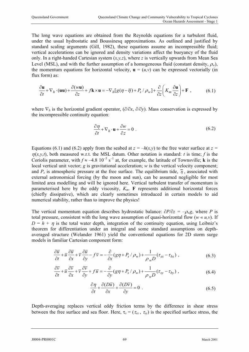
Queensland Government Queensland Climate Change and Community Vulnerability to Tropical CyclonesOcean Hazards Assessment - Stage 1
The long wave equations are obtained from the Reynolds equations for a turbulent fluid, under the usual hydrostatic and Boussinesq approximations. As outlined and justified by standard scaling arguments (Gill, 1982), these equations assume an incompressible fluid; vertical accelerations can be ignored and density variations affect the buoyancy of the fluid only. In a right-handed Cartesian system (x,y,z), where z is vertically upwards from Mean Sea
Level (MSL), and with the further assumption of a homogeneous fluid (constant density, w),the momentum equations for horizontal velocity, u = (u,v) can be expressed vectorially (in flux form) as:
( )( ) [ ( ) / ]h h s w
wf g P K
t z z
u uuu k u Fm
z
u, (6.1)
where h is the horizontal gradient operator, ( / x, / y). Mass conservation is expressed by the incompressible continuity equation:
0h
w
t zu . (6.2)
Equations (6.1) and (6.2) apply from the seabed at z = –h(x,y) to the free water surface at z =
(x,y,t), both measured w.r.t. the MSL datum. Other notation is standard: t is time; f is the
Coriolis parameter, with f –4.8 10–5 s–1 at, for example, the latitude of Townsville; k is thelocal vertical unit vector; g is gravitational acceleration; w is the vertical velocity component;and Ps is atmospheric pressure at the free surface. The equilibrium tide, , associated with
external astronomical forcing (by the moon and sun), can be assumed negligible for mostlimited area modelling and will be ignored here. Vertical turbulent transfer of momentum is parameterised here by the eddy viscosity, Km. F represents additional horizontal forces (chiefly dissipative), which are clearly sometimes introduced in certain models to aidnumerical stability, rather than to improve the physics!
The vertical momentum equation describes hydrostatic balance: P/ z = – wg, where P istotal pressure, consistent with the long wave assumption of quasi-horizontal flow (w « u,v). If
D = h + is the total water depth, integration of the continuity equation, using Leibniz’stheorem for differentiation under an integral and some standard assumptions on depth-averaged structure (Welander 1961) yield the conventional equations for 2D storm surgemodels in familiar Cartesian component form:
1( / ) ( )s w sx
w
u u uu v f v g P
t x y x Dbx , (6.3)
1( / ) ( )s w sy
w
v v vu v f u g P
t x y y Dby , (6.4)
( ) ( )0
Du Dv
t x y. (6.5)
Depth-averaging replaces vertical eddy friction terms by the difference in shear stress
between the free surface and sea floor. Here, s = ( sx , sy) is the specified surface stress, the
J0004-PR0001C 69 March 2001
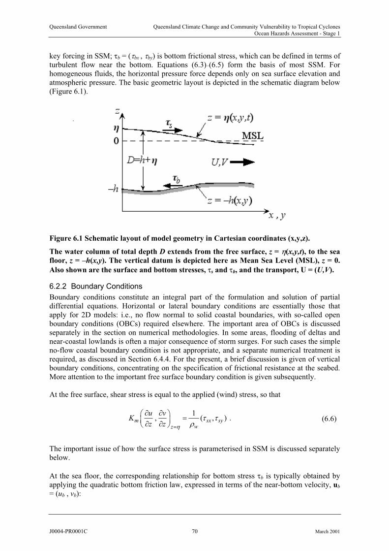
Queensland Government Queensland Climate Change and Community Vulnerability to Tropical CyclonesOcean Hazards Assessment - Stage 1
key forcing in SSM; b = ( bx , by) is bottom frictional stress, which can be defined in terms of turbulent flow near the bottom. Equations (6.3)–(6.5) form the basis of most SSM. For homogeneous fluids, the horizontal pressure force depends only on sea surface elevation andatmospheric pressure. The basic geometric layout is depicted in the schematic diagram below (Figure 6.1).
Figure 6.1 Schematic layout of model geometry in Cartesian coordinates (x,y,z).
The water column of total depth D extends from the free surface, z = (x,y,t), to the sea
floor, z = –h(x,y). The vertical datum is depicted here as Mean Sea Level (MSL), z = 0.
Also shown are the surface and bottom stresses, s and b, and the transport, U = (U,V).
6.2.2 Boundary Conditions
Boundary conditions constitute an integral part of the formulation and solution of partial differential equations. Horizontal or lateral boundary conditions are essentially those that apply for 2D models: i.e., no flow normal to solid coastal boundaries, with so-called open boundary conditions (OBCs) required elsewhere. The important area of OBCs is discussed separately in the section on numerical methodologies. In some areas, flooding of deltas and near-coastal lowlands is often a major consequence of storm surges. For such cases the simpleno-flow coastal boundary condition is not appropriate, and a separate numerical treatment is required, as discussed in Section 6.4.4. For the present, a brief discussion is given of vertical boundary conditions, concentrating on the specification of frictional resistance at the seabed. More attention to the important free surface boundary condition is given subsequently.
At the free surface, shear stress is equal to the applied (wind) stress, so that
1, (m s
wz
u vK
z z, )x sy . (6.6)
The important issue of how the surface stress is parameterised in SSM is discussed separatelybelow.
At the sea floor, the corresponding relationship for bottom stress b is typically obtained by applying the quadratic bottom friction law, expressed in terms of the near-bottom velocity, ub
= (ub , vb):
J0004-PR0001C 70 March 2001
Queensland Government Queensland Climate Change and Community Vulnerability to Tropical CyclonesOcean Hazards Assessment - Stage 1
1, ( , ) (m bx by b
wz h
u vK C
z zu , )b b bu v , (6.7)
where Cb is a quadratic bottom friction coefficient. Subscript b denotes values ‘near’ the bottom. In 3D numerical models, this is usually defined as the first grid point, at distance zb
above the seabed. Physically, Equation (6.7) should be consistent with the observed logarithmic velocity profile in the immediate vicinity of the seabed. Provided the vertical grid
can resolve this logarithmic sublayer, b can be expressed by the usual quadratic friction law, Equation (6.7), where the drag coefficient is then given by
2
0
1ln b
b
zC
z. (6.8)
Here, zb is the height of the first grid point above the sea floor, z0 is the aerodynamic
roughness length, and 0.4 is von Karman’s constant. The usual 2D parameterisation,which applies for Equations (6.3) and (6.4), is
( , ) ( ,b bx by f wC uu )v , (6.9)
where Cf is the friction factor appropriate to a depth-averaged treatment. For fully developed turbulence, Cf remains dependent on bottom roughness, in a manner described by, for example, the Colebrook-White formula (ASCE Task Force 1963),
101 14.8
4 2 logbf
D
kC. (6.10)
This is consistent with the definition of Cb in (6.8). A default value for the physical roughness height of kb 25 cm (so that z0 is of order 1 cm) is typical (Sobey et al. 1977, 1982). Note thatEquation (6.10) does model the increased influence of friction in shallow water, whereas common 2D modelling practice often simply sets Cf to a constant value, in the range 0.002–0.003. With kb = 25 cm, Cf values from (6.10) range from 0.0014 (D = 100 m) to 0.0033 (D = 2 m).
In the 2D case, however, the imposition of b is instantaneous, and hence this ignores thenatural frictional time scale Tf = O(h/Cf |u|), associated with momentum transfer through the water column. Suitable values for the passage of a tropical cyclone (hurricane) across a continental shelf (h = 50 m, Cf = 0.0025, |u| = 2 ms–1), yield Tf 3 h, which could be the sameorder as the time scale of the passage of the core of a moving hurricane. Equation (6.9) also ignores other 3D effects (Reid 1957). The simplest such example occurs for steady, linear wind-driven flow in a closed 1D channel, for which the depth-averaged velocity from
Equation (6.5) is u 0. From Equation (6.3), however, this implies that / x = ( s –
b)/( wgh). From Equation (6.9), the depth-averaged formulation gives b = 0. However, since
s 0, near-surface flow is directed by the wind stress, so that there must necessarily be a return flow, of opposite sign, near the bottom, in order to guarantee that u = 0. From the above
J0004-PR0001C 71 March 2001
Queensland Government Queensland Climate Change and Community Vulnerability to Tropical CyclonesOcean Hazards Assessment - Stage 1
expression for , surface and bottom stress contributions are additive for this case, so that water levels calculated from the zero depth-averaged velocity must under-estimate surface slope. Although such cases raise questions about overall validity, 2D models continue to be used widely and to generally perform well. This is especially so for computed water levels,which are largely insensitive to the vertical structure of the water column, even in 3D baroclinic models (Slordal et al. 1994).
6.2.3 Surge-tide Interactions
In many parts of the world, the presence of significant astronomical tides adds furthercomplications to storm surge dynamics (e.g., Bay of Bengal, North Sea, tropical Australia). Clearly, the relative phases of the surge and tidal components affect the peak sustained water levels, as seen to disastrous effect in Bangladesh (Flather 1994). It has long been recognised (e.g., Prandle and Wolf 1978, Heaps 1983) that simple superposition of these two components(i.e., ignoring their interaction), can lead to substantial errors in both the magnitude and timing of the peak surge. For the Queensland situation, these errors are expected to be muchsmaller due to the narrower continental shelf and the fewer regions with extensive flood plains.
The water depth, particularly in shallow waters significantly affects the nonlinear interactionof tide and surge. A further major contributor to this interaction is quadratic friction (Prandleand Wolf 1978). Consequently, simply adding the computed surge to the tide produces a conservative result for the total water level. In operational forecasting schemes, tidal andmeteorological forcing is now routine, and this practice has been standard over a long period of time in the SSM carried out at JCU (e.g., Stark et al., 1985).
6.3 External Forcing
The effects of surface pressure and, particularly, surface stress, are the principal agents that act to generate the storm surge. Atmospheric pressure acts on the entire water column,contributing to the barotropic dynamic pressure. Assuming atmospheric pressure is known accurately, its incorporation presents no problems for SSM. In the shallow waters of the continental shelf, the effects of the surface wind stress are so profound, yet so complex
physically, that the results of model calculations depend critically on the manner in which s
is specified. This has lately become an active area of research through incorporation of the effects of surface waves, a topic to which some attention is given below. For the present, we consider only the traditional method of parameterising surface stress in terms of the surface wind speed, but it is evident, even in this area, that many uncertainties remain.
6.3.1 Wind field modelling
The foremost requirement for SSM is an accurate wind field model, and the divide betweenthe mid-latitude and tropical cases is most pronounced here. Mid-latitude models take their wind (and pressure) fields from operational NWP models, which generally perform well. Current developments involve the use of finer-scale meteorological models (e.g., Gerritsen et
al. 1995, Vested et al. 1995). The same does not apply for tropical cyclones, where the task of path and intensity prediction remains an active and developing field (e.g., Kurihara et al.,1995). Some sophisticated predictive modelling has been attempted, using moving nestedgrids and assimilated data from storm-penetrating aircraft, but such work is still experimentaland is likely to remain beyond the operational capabilities of most areas subject to tropical
J0004-PR0001C 72 March 2001
Queensland Government Queensland Climate Change and Community Vulnerability to Tropical CyclonesOcean Hazards Assessment - Stage 1
cyclones. Tropical SSM relies on synthetic wind and pressure field models, of a relatively simple nature, characterised by a small set of parameters.
Computed responses of the ocean are found to be critically dependent on a tropical cyclone’s velocity of forward movement, Vfm, both in the deep ocean (Price et al. 1994) and over the continental shelf (Sobey et al. 1977, Fandry and Steedman 1994). The storm track is influenced by synoptic-scale meteorology, but the tropical cyclone also generates its own self-steering mechanisms, due to interactions between its intense vorticity field and the meridionally varying planetary vorticity field in which it is embedded (Chan and Williams,1987). Despite this, the practical modelling issues of cyclonic wind and pressure fields for tropical SSM are generally limited to the simplified parametric models described earlier inChapter 5. Obtaining sufficiently accurate values for these parameters is another matter,although advances in remote sensing offer increasingly improved estimates.
Hydrodynamic forcing is due to the transfer of momentum to the marine boundary layer (BL)
from the frictional inflow surface layer of the tropical cyclone. Surface wind shear stress s
and atmospheric pressure Ps act on the water body across massive scales, generating complexforced and free modes of motion, which can persist for days after a storm.
The considerable uncertainty that accompanies the specification of the tropical cyclonevelocity field, Vm, is evidenced by the prescriptive nature of such formulations. Thisuncertainty must automatically be transferred, through further assumptions about air-sea interaction processes, to the storm surge models. Given the lack of detailed knowledge of thetropical cyclone BL, it is perhaps not surprising that such simple and empirical approacheshave been adopted. Nevertheless, there is wide agreement that the correct specification of wind speed is a crucial first step in providing forcing to storm surge models (Heaps 1983, Proctor and Wolf 1990, Hardy et al., 2000). The present approach remains a weak link in the overall parameterisation of the physics of tropical SSM.
Extensive use has been made of the Holland (1980) profile in storm surge and wave modelling on the North West Shelf of Western Australia (Harper et al. 1993). Approximately30 cyclones were hindcast, using objectively analysed best estimates of the storm tracks. The main parameter varied was Holland’s peakedness factor, B, with some tuning of the reported R (radius to maximum winds) value also used. Many of these hindcasts were able to fit the measured data extremely well (see Figure 1 in Bode and Hardy, 1997) for intense tropical cyclone Orson, of April 1989, in which a minimum central pressure of 905 hPa was recorded.Excellent agreement between measured and modelled winds at one of the anemometer siteswas observed; the fit to data at six other sites was almost equally convincing. The best-fit value of the B factor for Orson was B = 1.94.
6.3.2 Parameterisation of surface stress
Assuming the wind field is adequately known, the final step in specifying atmospheric forcing for most storm surge models is the calculation of surface shear stress via the quadratic drag law:
10 10 10( , )s sx sy aC U U . (6.11)
J0004-PR0001C 73 March 2001
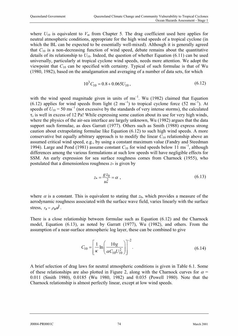
Queensland Government Queensland Climate Change and Community Vulnerability to Tropical CyclonesOcean Hazards Assessment - Stage 1
where U10 is equivalent to Vm from Chapter 5. The drag coefficient used here applies for neutral atmospheric conditions, appropriate for the high wind speeds of a tropical cyclone (inwhich the BL can be expected to be essentially well-mixed). Although it is generally agreed that C10 is a non-decreasing function of wind speed, debate remains about the quantitativedetails of its relationship to U10. Indeed, the question of whether Equation (6.11) can be used universally, particularly at tropical cyclone wind speeds, needs more attention. We adopt the viewpoint that C10 can be specified with certainty. Typical of such formulae is that of Wu(1980, 1982), based on the amalgamation and averaging of a number of data sets, for which
310 1010 0.8 0.065C U , (6.12)
with the wind speed magnitude given in units of ms–1. Wu (1982) claimed that Equation (6.12) applies for wind speeds from light (2 ms–1) to tropical cyclone force (52 ms–1). At speeds of U10 = 50 ms–1 (not excessive by the standards of very intense storms), the calculated
s is well in excess of 12 Pa! While expressing some caution about its use for very high winds,where the physics of the air-sea interface are largely unknown, Wu (1982) argues that the data support such formulae, as does Garratt (1977). Others such as Smith (1988) express strongcaution about extrapolating formulae like Equation (6.12) to such high wind speeds. A moreconservative but equally arbitrary approach is to modify the linear C10 relationship above an assumed critical wind speed, e.g., by using a constant maximum value (Fandry and Steedman1994). Large and Pond (1981) assume constant C10 for wind speeds below 11 ms–1, although differences among the various formulations at such low speeds will have negligible effects for SSM. An early expression for sea surface roughness comes from Charnock (1955), who postulated that a dimensionless roughness z* is given by
0* 2
*
g zz
u, (6.13)
where is a constant. This is equivalent to stating that z0, which provides a measure of theaerodynamic roughness associated with the surface wave field, varies linearly with the surface
stress, .s au*2
There is a close relationship between formulae such as Equation (6.12) and the Charnock model, Equation (6.13), as noted by Garratt (1977), Wu (1982), and others. From the assumption of a near-surface atmospheric log layer, these can be combined to give
2
10 210 10
1 10ln
gC
C U. (6.14)
A brief selection of drag laws for neutral atmospheric conditions is given in Table 6.1. Some
of these relationships are also plotted in Figure 2, along with the Charnock curves for = 0.011 (Smith 1980), 0.0185 (Wu 1980, 1982) and 0.035 (Powell 1980). Note that the Charnock relationship is almost perfectly linear, except at low wind speeds.
J0004-PR0001C 74 March 2001

Queensland Government Queensland Climate Change and Community Vulnerability to Tropical CyclonesOcean Hazards Assessment - Stage 1
Figure 6.2 C10 as a function of U10 for formulations 1, 4 and 5 of Table 6.1.
Dashed curves show the Charnock formulation for constant : (i) = 0.011,
(ii) = 0.0185, (iii) = 0.035.
Table 6.1 Various formulations for surface drag coefficient C10
Investigators 103C10 Range (ms
-1)
1.Smith and Banke (1975) 0.63 + 0.065U10 3 U10 21
2. Garratt (1977) 0.75 + 0.067U10 4 U10 21 0.017
3. Smith (1980) 0.61 + 0.063U10 6 U10 22 0.011
4. Wu (1982) 0.80 + 0.065U10 2 U10 0.0185
5. Large and Pond (1981) 1.2 4 U10 11
0.49 + 0.065U10 U10 26
J0004-PR0001C 75 March 2001

Queensland Government Queensland Climate Change and Community Vulnerability to Tropical CyclonesOcean Hazards Assessment - Stage 1
6.4 Solution Procedures
Numerical solution procedures are obligatory for realistic SSM. Closed form solutions in anyrealistic geometry to the 2D equations (6.3)–(6.5), are out of the question, and numericalmethods are essential. Details of numerical procedures are available in the literature, and only the barest details are offered here, although we do address the important subject of openboundary conditions (OBCs). We note also the important role of solutions that use idealised shelf geometries, both analytical and numerical. In spite of their limitations, these illustratesome of the essential dynamical aspects of storm surge response. Three recent numericalworks can be consulted for details: Fandry and Steedman (1994) discuss various aspects ofidealised 2D storm surge response; Tang and Grimshaw (1995) use a mode fitting analysis to study barotropic storm-generated continental shelf waves; and Slordal et al. (1994) model the baroclinic response on a deep continental shelf, for which the dominant response is in the currents due to shelf waves.
Whether 2D or 3D models are used, the numerical solution of the equations of motion essentially comprises a coupled set of 2D (horizontal) equations. The particular algorithm used can be chosen from a myriad of available methods. A number of significant questions then arise, including whether to use a finite difference (FD) or finite element (FE) algorithm.This choice almost invariably influences the nature of the spatial discretisation and the arealextent of the model domain, with consequent impact on the representation of OBCs. The time differencing scheme may be explicit or implicit. Other topics, such as the treatment of the nonlinear advective terms (simple scaling shows these should not be ignored for the extremesof tropical cyclone forcing), lead to a further range of numerical representations, beyond the scope of this review.
6.4.1 Finite Difference versus Finite Element
Much has been written on the formulation (and relative merits) of FD and FE solutions to the long wave equations. Works where specific details and summaries can be found include Abbott and Basco (1989), Foreman (1984), Haltiner and Williams (1980), Heaps (1983), and Murty (1984). Both methods produce large sets of matrix equations, and grids with 105 or more unknowns are no longer uncommon. In FD schemes, grids are generally rectangular; larger-domain models should be formulated in spherical polar coordinates (Flather, 1994). In general, the staggered Arakawa ‘C’ spatial grid is used (Mesinger and Arakawa 1976), allowing easy imposition of the zero normal flow coastal boundary condition. Increased spatial resolution in key areas (e.g. inlets) has been claimed through the use of stretched and curvilinear grid systems, although they can introduce unusual open boundary geometry.Similar techniques have been used to transform irregular coastlines onto rectangular horizontal model domains (Reid et al. 1977, Johns et al. 1981, Bentsen et al. 1999). FE equations are invariably derived via a Galerkin approach (Foreman 1984), and tend to use triangular grids to conform with irregularly shaped boundaries and to selectively enhance spatial resolution. FE triangulations are usually generated semi-automatically by specialised software – Henry and Walters (1993).
Finite element SSM is relative new. Such methods first solved the primitive equations (6.3)–
(6.5) (Taylor and Davis 1975). Thacker (1978) argued that on the grounds of computationaleconomy, FE methods were uncompetitive with FDs, but a more fundamental concern was the generation of noisy solutions. This originated from the nature of the numerical wave
J0004-PR0001C 76 March 2001
Queensland Government Queensland Climate Change and Community Vulnerability to Tropical CyclonesOcean Hazards Assessment - Stage 1
dispersion relationship for primitive equation FEs (Lynch and Gray, 1979), thereby givingpossible multiple solutions. Lynch and Gray recast the problem in the form of a generalisedwave equation to remove the noise problem (Foreman 1984). The wave equation approach is now the dominant method for FE models. Near-coastal 3D models are still almost exclusively cast in FD form (Blumberg and Mellor, 1987). Both FD and FE methods are valid approaches, and no fundamental advantage should necessarily be ascribed to either one or the other, despite some partisan claims in the literature. However, FD methods have so far been the predominant choice in SSM, dating from the pioneering efforts of Hansen (1956), and continued by Jelesnianski (1965), Leendertse (1967), Reid and Bodine (1968), and manyothers.
6.4.2 Explicit vs Implicit
The simplicity of explicit time differencing schemes has seen them retain their popularity for SSM, despite an increase in the use of implicit methods. The discussion here concentrates on the simpler FD schemes. FE methods, although inherently implicit, can also be formulated explicitly (Foreman 1984). Explicit methods lead to simple time-stepping schemes; the mainadvantage is the ease and speed with which error-free code can be produced. Their obvious shortcoming lies with the CFL criterion, which for the 2D case is given by
max2
st
gD, (6.15)
with t the time step and Dmax the maximum depth. Thus for explicit 2D models, not only is
t ~1 Dmax , but (6.15) also implies the total CPU time, TCPU ~ N3, where N is the total
number of active grid cells (with TCPU ~ N 4 for 3D models). Simple arithmetic thus shows that timesteps for high-resolution FD models can be extremely restrictive if, as is ideal, themodel domain extends into deep water. JCU experience has concentrated on problems in the GBR, with a consequent need for relatively fine spatial grids, and all models have been converted to implicit methods (Bode and Mason 1994). This is despite the fact that earlier modelling (Sobey et al., 1977) used explicit schemes exclusively.
Implicit models are not in general bound by stability criteria such as Equation (6.15), but we stress the need to consider model accuracy as the prime requirement, rather than stability.Inverting large matrices is required in implicit models, and although they are extremely sparse and highly structured, the resulting computational task is usually very demanding. Early implicit models favoured the alternating direction implicit (ADI) algorithm (Leendertse 1967), with its need to invert only tridiagonal matrices. However, ADI can lead to problemsin regions of complex geometry (Wilders et al. 1988), and semi-implicit and fully implicitmodels are being adopted more widely. Traditional methods for matrix inversion such as successive over-relaxation, although simple to implement, suffer from prohibitively slowconvergence rates for large problems. Advantage can be taken of operator splitting, and the adoption of more modern sparse matrix techniques, such as pre-conditioned conjugate gradients (Wilders et al. 1988, Bode and Mason 1994) and multigrid methods. In semi-implicit methods, the critical timestep restriction Equation (6.15) is removed through implicitformulation of the gravity wave terms.
J0004-PR0001C 77 March 2001
Queensland Government Queensland Climate Change and Community Vulnerability to Tropical CyclonesOcean Hazards Assessment - Stage 1
In early models, the lack of CPU resources led to a need for relatively coarse grids, and modeldomains that were limited in spatial extent. The constraint applied by Equation (6.15) wasthus not excessive and, with the accompanying ease of programming, made explicit methodsan attractive option. Increasingly now, high spatial resolution is demanded, while is it alsoclear that model domains should be made as large as possible to aid with the problems of
OBCs (below). The resulting minuscule values of t demanded by Equation (6.15) now makeimplicit modelling much more attractive, in spite of its inherent complexity. For high
resolution grids, it has been shown in certain circumstances that t values, many times thetraditional CFL limit, can be used while still retaining stability and accuracy (Wilders et al.
1988, Bode and Mason 1994). Clearly, there is a trade-off between small t values for explicitmodels and the cost of matrix inversion in the implicit case.
6.4.3 Sizes for spatial step and time step
Standard application of Fourier analysis to numerical schemes for the long wave equations (e.g., Abbott and Basco 1989) leads to a resolution criterion that states approximately
20
Ls . (6.16)
Here, s and L are representative length scales for the numerical grid resolution and the shortest inertia-gravity wavelengths expected to be generated by the storm (or tides). Thisessentially states that the long waves must be sufficiently well resolved by the grid (i.e., by 20 grid points or better per wavelength). Provided this rule-of-thumb is adhered to, few problems
should be expected in numerical integrations, especially in the calculation of water levels, .Note, however, that additional length scale criteria are imposed in the coastal SSM problem.
The model must be capable of resolving the following:
(i) The strong spatial gradients in the cyclone wind field cause rapid spatial changes in magnitude and direction of surface stress. The band of maximum winds can reverse direction over a distance equal to about twice the radius to maximum winds of the cyclone. This indicates that the appropriate ocean response wavelength should be set at four times the radius. This is also consistent with the need to resolve the surface wind
gradients, as highlighted by Sobey et al. (1977) who suggested R/ s > 4 as a suitable rulefor preserving the forcing wavelength.
(ii) The gradient of water surface elevation is largest in shallow water and the primaryinterest of SSM is to provide coastal surge values. If the computational point nearest to the actual shoreline is some distance offshore, the surge may be underpredicted, since this gradient will not apply all the way to the true shoreline location. Likewise, the surgewould be overpredicted if the grid point were onshore from the true shoreline position.Simplifying Equation (6.3) to 1D, steady state, and ignoring pressure and Coriolis
effects, the gradient of the surface elevation is approximately 2 10-4 for a wind speed of 50 ms-1 normal to shore and a water depth of 4 m. Thus if the grid point is 1000 m
offshore, the surge is underpredicted by approximately 0.2 m (2 10-4 1000 m = 0.2 m).
(iii) Coastal features such as headlands, islands or shoals and channels can trap and or direct water movements, thus changing coastal surge levels.
J0004-PR0001C 78 March 2001
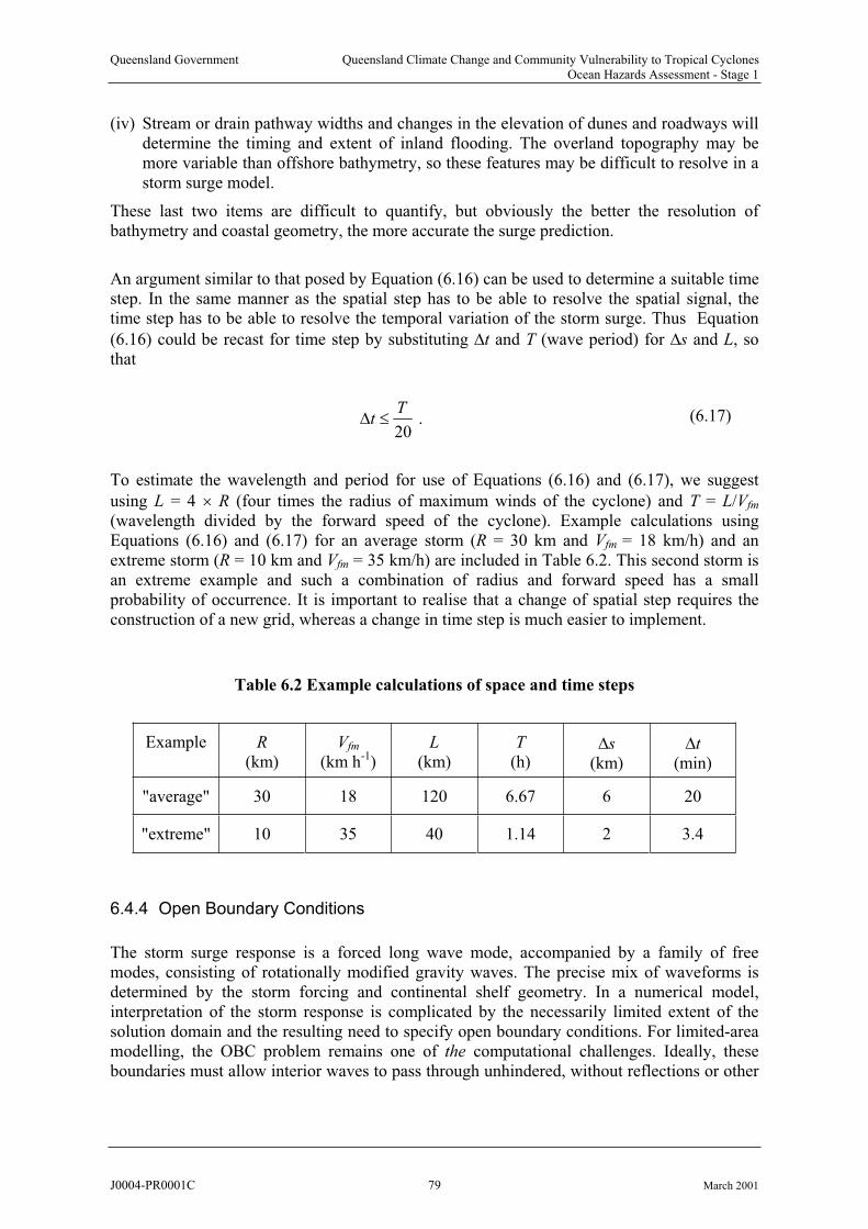
Queensland Government Queensland Climate Change and Community Vulnerability to Tropical CyclonesOcean Hazards Assessment - Stage 1
(iv) Stream or drain pathway widths and changes in the elevation of dunes and roadways will determine the timing and extent of inland flooding. The overland topography may be more variable than offshore bathymetry, so these features may be difficult to resolve in a storm surge model.
These last two items are difficult to quantify, but obviously the better the resolution of bathymetry and coastal geometry, the more accurate the surge prediction.
An argument similar to that posed by Equation (6.16) can be used to determine a suitable timestep. In the same manner as the spatial step has to be able to resolve the spatial signal, thetime step has to be able to resolve the temporal variation of the storm surge. Thus Equation
(6.16) could be recast for time step by substituting t and T (wave period) for s and L, so that
20
Tt . (6.17)
To estimate the wavelength and period for use of Equations (6.16) and (6.17), we suggest
using L = 4 R (four times the radius of maximum winds of the cyclone) and T = L/Vfm
(wavelength divided by the forward speed of the cyclone). Example calculations usingEquations (6.16) and (6.17) for an average storm (R = 30 km and Vfm = 18 km/h) and an extreme storm (R = 10 km and Vfm = 35 km/h) are included in Table 6.2. This second storm is an extreme example and such a combination of radius and forward speed has a smallprobability of occurrence. It is important to realise that a change of spatial step requires theconstruction of a new grid, whereas a change in time step is much easier to implement.
Table 6.2 Example calculations of space and time steps
Example R(km)
Vfm
(km h-1)L
(km)T
(h)s
(km)t
(min)
"average" 30 18 120 6.67 6 20
"extreme" 10 35 40 1.14 2 3.4
6.4.4 Open Boundary Conditions
The storm surge response is a forced long wave mode, accompanied by a family of freemodes, consisting of rotationally modified gravity waves. The precise mix of waveforms is determined by the storm forcing and continental shelf geometry. In a numerical model,interpretation of the storm response is complicated by the necessarily limited extent of thesolution domain and the resulting need to specify open boundary conditions. For limited-areamodelling, the OBC problem remains one of the computational challenges. Ideally, these boundaries must allow interior waves to pass through unhindered, without reflections or other
J0004-PR0001C 79 March 2001
Queensland Government Queensland Climate Change and Community Vulnerability to Tropical CyclonesOcean Hazards Assessment - Stage 1
unrealistic behaviour; additionally, they should also permit any information associated with external forcing to pass into the region.
The true open coast situation is one where OBCs can exert an identifiable impact on the computed solution. In general, such models have two transverse or cross-shelf open boundaries, and one in deep water off the shelf edge. The first step along all boundaries should be to incorporate the inverted barometer effect. Atmospheric pressure can essentially be removed from the momentum equations (6.3) and (6.4) by defining an adjusted sea level elevation,
w
P
g, (6.18)
where P = (pn – ps) is the local atmospheric pressure deficit. This gives the well-known rule that a 1 hPa pressure drop leads approximately to a 1 cm rise in static sea level. From
Equation (6.3) or (6.4), the ratio of surface stress to atmospheric pressure forcing is O( s L/(D
P)), where L is a length scale for horizontal pressure variations (e.g., 400 km). For parameters appropriate to strong hurricanes such as Camille (Table 1, Bode and Hardy 1997), this ratio is of the order of 10 for h = 20 m, but only 0.01 for h = 2,000 m. The dominatinginfluence in deep water of the inverted barometer effect is obvious in many modelling studies
from the near-circular -contours which mirror the radially symmetric form of ps that is oftenimposed for idealised storms (Bunpapong et al. 1985, Blain et al. 1994, Fandry and Steedman1994). Given the importance of surge-tide interactions, tidal elevations are also generally added to the OBCs; this is largely a routine matter.
On transverse boundaries, however, the use of Equation (6.18) plus tidal modifications is insufficient. Unless OBCs are further modified, they will act along these cross-shelf boundaries to produce total internal reflection of any waves generated within the modeldomain (subtraction of the forced tidal and inverse barometer solutions means that such
models effectively apply a condition of zero elevation). Instead of this ‘clamped’ ( ' = 0) OBC, Jelesnianski (1965) and Forristall (1974), adopted a condition of zero normal velocity derivative along transverse open boundaries – e.g., for an x-directed boundary,
0v
y.
(6.19)
Either the clamped condition or Equation (6.19) is computationally trivial to apply, but both were shown by Reid (1975) to produce total internal reflection of wave energy, thus preventing free modes from passing unrestricted out of the model region. Reid advocated a‘radiation’ condition and showed that for 1D gravity waves, these internal reflections are prevented if the velocity and surface elevation are in phase, as with a travelling wave. Specifically, the Reid radiation condition is
cv
D, (6.20)
a condition originating with Reid and Bodine (1968). The default value for the velocity is the celerity of free gravity waves, c = (gD)1/2, the sign depending on the direction of the outward
J0004-PR0001C 80 March 2001
Queensland Government Queensland Climate Change and Community Vulnerability to Tropical CyclonesOcean Hazards Assessment - Stage 1
normal. Modifications for combined tidal and surge modelling are given in Flather (1981). Strictly, (6.20) allows progressive waves in the computational domain to pass through the open boundaries in the absence of forcing and rotation (f = 0), and with quiescent initialconditions. Problems with the performance of Equation (6.20) on cross-shelf boundaries for steady wind-driven shelf flow (Bode and Sobey 1983), have led to the adoption of the kinematic ‘Sommerfeld’ condition (Orlanski 1976):
0ct x
, (6.21)
where denotes any variable to be ‘radiated’ through the boundary, and c is a suitablevelocity. A number of such schemes, chiefly involving variations in the definition of c, are investigated by Chapman (1985). Further variants of Equation (6.21) are described by Tang and Grimshaw (1996), whose main concern was to ensure the correct propagation ofcontinental shelf waves.
Another approach is the Flow Relaxation Scheme (FRS) of Martinsen and Engedahl (1987). It blends the results of fine-scale, near coastal models with those from larger domain externalmodels, in which the fine-scale model is nested, according to the ‘convex combination’:
(1 )ext nt , (6.22)
where is the relaxation parameter (0 < < 1). Martinsen and Engedahl (1987) show that FRS performs well on nested problems, and can also be used as a pure OBC. OBCs continue to exercise the interest of modellers, but as summarised by Chapman (1985), the fact remainsthat for wind-driven flows, no OBC performs satisfactorily in a general sense for open coast wind-driven models. If these are to be used, then experimentation and compromise areessential.
Tropical cyclone SSM leads to an essential conflict of scales that affects OBCs: at one extreme, the storm’s eye radius (the scale of the dominant forcing) together with prominentcoastal and bathymetric features must be resolved adequately; at the other, the model domainshould encompass the extent of the storm. Ideally, a model should accommodate both ends of this spectrum (even now an often-impossible demand with realistic CPU resources), and the compromise of limited-area models and OBC problems are usually an immediate consequence. Non-uniform grids, as used by the FE modellers offer one solution, as doboundary-fitted and other transformed mesh approaches for FDs. If fixed resolution FD grids apply, recourse should be made to nested grids (Haltiner and Williams 1980), using methodssuch as FRS to couple the boundary interfaces. Multiple-stage nesting provides an effective and affordable means of obtaining extra accuracy at smaller scales, especially for the regionsof major interest near coastlines, while still incorporating the effects of distant forcing in thedeep ocean, where resolution requirements are not so crucial.
Despite efforts expended to develop artificial OBCs, model studies show that the ideal way to minimise the problem is to use as large a domain as possible. This can be seen as a further reason to opt for a nested approach, with a cheap outer grid of maximum possible extent. Both Bunpapong et al. (1985) and Blain et al. (1994) consider the storm surge problem for tropical cyclones in the Gulf of Mexico. Blain et al. used three grids of increasing size. The smallestcovered a region with an extent of 175 km, corresponding to the local SLOSH model grid
J0004-PR0001C 81 March 2001
Queensland Government Queensland Climate Change and Community Vulnerability to Tropical CyclonesOcean Hazards Assessment - Stage 1
(Jelesnianski et al. 1992). The second encompassed the entire Gulf, while the third extended into the Caribbean and the eastern US shelf. The results support those of Bunpapong et al.
(1985), who showed the importance of the natural modes of oscillation of the Gulf to the storm surge response. Minor differences were found between results for the two larger grids, both of which produce significantly higher coastal water levels than for the SLOSH grid. Jarvinen and Lawrence (1985) also comment that the extent of the SLOSH grid is far too limited for use in operational modelling.
6.4.5 Overland Flooding and Drying
The ‘standard’ coastal boundary condition used in long wave models is that of no flow at thecoastline, i.e., the component of transport normal to the coastline equals zero. Thus, this boundary condition essentially approximates the coast by a vertical cliff of unlimited height,
against which the free surface water level, , can rise and fall. Quite apart from the fact thatall models can only approximate the position of the coastline (e.g., that corresponding toMSL), the topography there often changes gradually, not abruptly. In addition, many coastal regions are bordered by low-lying land: tidal flats such as those adjacent to parts of ClevelandBay; large stretches of coastal plains close to sea level, such as those bordering the Gulf of Carpentaria; and inter-tidal lagoons and embayments. All may be subject to inundation attimes of high astronomical tides or during a storm surge.
Thus, an important component of many coastal hydrodynamic models is the existence of modules to compute the extent of such incursions of seawater. These are often labelled wetting/drying or flooding algorithms. Such schemes will necessarily include a database ofon-shore topography, at least for regions deemed flood-prone. The model must then computethe progress of the water across such areas – both the position of the wet/dry interface, and the depth of water in all ‘wet’ computational cells. This is not a simple problem. Indeed, the fact that various schemes are still being proposed in the recent modelling literature, is a strong indication that flooding and drying is not a closed issue.
Flooding and drying – modelling approaches
Two immediate and separate formulations suggest themselves for flooding and drying. The more natural one is to compute the position of the interface, which is tracked adaptively by a grid that changes over time. With this approach, grid cells can move or be added at the wet/dry interface at each time step. Computationally, this is a most demanding problem, as it requires continual regridding. In fact, even strong protagonists of finite element schemes(which in principle can be regridded to closely follow the evolving coastline) avoid this method; such are the computational difficulties and prohibitive CPU overheads. The second scheme operates with a fixed grid, in which all points can be either wet or dry at any timestep;in fact, this disjunction will usually only arise over a small fraction of the grid. In theory, agrid cell adjacent to a wet cell in which water has risen in the previous timestep to a level above its own base level, can become wet during the next timestep. In practice, this transition causes quite severe numerical problems.
What is commonly seen is a type of shock wave effect, due to the fact that cells flood and become instantaneously active (wet) – or else passive (dry) during the retreat of a flood.Numerically, this situation is often characterised by noisy solutions near the coastline, and a tendency for such models to become catastrophically unstable. One of the difficulties is that,under such conditions, the dynamics change markedly: from a long wave in which pressure
J0004-PR0001C 82 March 2001
Queensland Government Queensland Climate Change and Community Vulnerability to Tropical CyclonesOcean Hazards Assessment - Stage 1
gradient and inertial terms are in approximate balance and friction is weak, to a very shallow water situation in which bottom friction provides the dominant balance for pressure forces. This was recognised by LeBlond (1978). He showed that in such situations, for 1D flow in a channel, the dynamics change from a wave equation with two characteristics, to a nonlinear diffusion equation with a single characteristic. Under 2D flow conditions, such problems are naturally far more complicated, especially when the advective terms are applied.
Despite this, most modellers have proceeded to treat the wetting and drying problem in abasically conventional fashion, using a standard long wave model, and employing various additional methods to prevent drastic temporal changes from occurring near the interface. Early work of this type included that by Leendertse (1970), and Flather and Heaps (1975). Later modifications, in which the equations for the wetted grid cells were modified to buffer the impacts of the encroaching interface, include Flather and Hubbert (1990). Other approaches to the problem include the use of weir formulae (Reid and Bodine, 1968; Sobey et
al. 1982), and barriers along the boundaries of grid cells that can be added or removed to alter the progress of the flood wave. None can really be said to have “solved” the problem.
More recently, Hubbert and McInnes (1999), who employ explicit numerics in their stormsurge model, report a scheme which seeks to limit the rate of flooding and drying of active grid cells. Under their methodology, an attempt is made to compute an appropriate approach or retreat velocity of the flood wave front over a number of timesteps in adjacent (wet) grid cells. They use this technique to reduce the noise generated by the continual switching of grid cells from active to passive, and vice versa. By comparison of the results against those from a rigid coastline model, Hubbert and McInnes claim that their scheme “ensures realistic and smoothly varying results”. They concluded that fixed coastline models could lead to a significant over-estimation of the magnitude of the maximum surge at the coast. However,lack of detailed inundation data (a general problem with such assessments) allowed them to perform only a qualitative analysis of their flooding algorithm. At best they could say that the area of land inundated in the model was similar to that observed. No measurements of inundation water heights or water speeds were available to make any detailed calibrations ofthe model.
Flather (1994) has developed a novel approach to the flooding problem for the very extensive Bangladesh delta region, a region often hit by storm surges, with devastating losses of life and property. This extended earlier work by Flather and Hubbert (1990). The region is traversed by numerous river channels of a variety of sizes. In order to incorporate both the inundation of land and flow in river channels, Flather developed a hybrid 1D/2D system, within the overall context of a 2D model, using a variety of partial area and width factors. This attempt torepresent sub-grid-scale effects is in some senses similar to the JCU reef parameterisationscheme (Bode et al., 1997). The procedure appeared to be effective numerically. However, again there were no essentially no detailed data to allow adequate comparisons with reality. A linked 1D/2D approach is also utilised by a number of commercially available river floodplain models, such as those by Delft Hydraulics and the Danish Hydraulic Institute, and good verification against recorded terrestrial flood events is claimed.
Ip et al. (1998) adopt a significantly different approach, and revert to the friction-pressure gradient balance, initially demonstrated by LeBlond (1978) for flow in shallow tidal rivers. They combine this with a porous sublayer in cells that can become wet, in order to smooth the potentially troublesome temporal variations in water level. Their method seems to offerconsiderable promise (in part at least because it operates under the correct dynamical regime).
J0004-PR0001C 83 March 2001
Queensland Government Queensland Climate Change and Community Vulnerability to Tropical CyclonesOcean Hazards Assessment - Stage 1
However, this approach would require considerable further development if it were to beproposed for an operational storm surge model. In the work they report, Ip et al. (1998) limitthemselves to very near coastal situations, such as modelling the flooding of inter-tidal areas. For successful implementation in a storm surge model, their scheme would have to be interfaced across a transition zone to the main deepwater region of the model, where long wave dynamics apply.
In order to avoid instability in the switching between flooding and drying, the flood/drying scheme in MMUSURGE maintains a finite water depth (set to a very small value) in all cellswhere flooding is possible. In effect, there is no “drying” of cells. Although this avoids the instability problem, in an implicit model (such as MMUSURGE), the development of a flooding scheme is complicated by the significantly longer timesteps that are commonly used in implicit models. The highly nonlinear nature of the overland flooding process means that implicit models should have time steps that give Courant numbers number close to one in regions of overland flooding. However, time steps have already been reduced in order to
resolve the forcing of a tropical cyclone. For example, with t = 900 s, s = 925 m, theCourant number is less than about 3 for water depths indicative of the flood front over dry
ground (less than a about 1 m). Further, the value of L/ s remains above the threshold figure of 20 in equation (6.16) for a storm with a time scale of around 3 hours. Both of these should ensure that the numerical scheme satisfactorily describes the dynamical situation (Bode and Mason, 1994).
There are additional aspects of the storm surge flooding problem that require consideration.For example, very shallow flow of water over the land affects the determination of (i) bottomfriction, and (ii) wind stress on water. Bottom friction will be enhanced by vegetation,housing and other roughness elements, far larger in physical extent than the few cm usually assumed for flow over the sea floor – with the exception of the GBR. Wind stress applied to the water surface, over what is nominally land, would tend to be reduced because of trees andother obstacles. On the other hand, certain situations would allow the application of a large surface stress to extensive regions of very shallow water (see below). At present,MMUSURGE uses a spatially constant value of bottom roughness. Thus the increased roughness of flooded areas, which are very different from the ocean floor, is not well represented. A spatial varying value of roughness can be simply incorporated into the calculation scheme. This is recommended if modelling of overland flooding is to be an important component of future projects.
Two separate cases apply to the overland flooding problem for Queensland. The first is the situation in the Gulf of Carpenteria, where the flood wave must move long distances over relatively featureless terrain. The second is low-lying populated areas (on the scale of a single suburb). Here the flood wave does not travel large distances, but must negotiate a very complicated flood path around obstacles, such as curbs, walls and houses. The first requires moderately accurate terrain information and adjustable bottom friction coefficients over theflooded area. The accuracy and obtainability of this data is the main problem. The second requires very fine scale descriptions of structures and needs much finer grid resolution. This very fine resolution is clearly impractical for the present purpose of modelling storm surge for the entire coast of Queensland. The alternative is to include sub-grid scale algorithms, in much the same way as MMUSURGE does for reef features (Bode et al., 1997). Thus, these small-scale features are accounted for with a much larger spatial step size. This is clearly the only way the overland flooding can be modelled for anything but a very small region (a suburb or smaller). It is important to realise that these small-scale features may change (new
J0004-PR0001C 84 March 2001

Queensland Government Queensland Climate Change and Community Vulnerability to Tropical CyclonesOcean Hazards Assessment - Stage 1
road, wall, or growth of vegetation) or even dynamically during a storm (i.e. erosion of dunesor change in channel).
A very important consideration in overland flooding is the need to know the total water level,which means that the simultaneous modelling of surge and tide is necessary. This addsconsiderably to the cost of modelling over that of the open coast where a superposition of tide and surge (perhaps with some adjustment) is possible.
In summary, while overland flooding is not important in many areas it is clearly an important issue in some locations. However, there remain significant difficulties in providing reliableflooding schemes, as well as accommodating their computational overheads.
6.5 Recent Developments
Accurate forecasting of storm surge is critically dependent on the quality of many modelinputs and parameters. Especially important among these are: meteorological forcing and the parameterisation of air-sea interaction; open boundary conditions; bottom friction andbathymetry. Errors in any of these may lead to a marked deterioration in numerical results.Recent developments in a number of areas of ocean modelling have opened possibilities for distinct improvements in storm surge model predictions. Most of these are in their infancy as evidenced by the recent dates of the references cited. For the present, we focus here ondevelopments in coupled surge-wave models. Another area of innovation covered by Bodeand Hardy (1997) is the use of inverse methods, notably for data assimilation, a field of study that is currently undergoing rapid evolution in theoretical meteorology and oceanography.
6.5.1 Surge-Wave Interactions
At the time of the Heaps (1983) review, nonlinear surge-tide interactions were being incorporated in SSM. The chief agent of interaction there is bottom friction. It is equallyrecognised that specifying surface stress as a function of only the wind speed, underestimatesthe vital role that surface wind waves play in the transfer of momentum at the air-sea interface, particularly under the complex action of tropical cyclone wind fields. This interaction has been ignored in the past, and storm surge and waves have usually been studied and modelled in isolation. In this section we consider the effects of waves on sustained water levels. These interactions occur through at least three mechanisms – radiation stress, enhanced bottom stress, and enhanced surface wind stress. The last mechanism is the major focus of this section.
It is well known (Longuet-Higgins and Stewart, 1964) that waves cause a flow of momentum,and a spatial gradient in this momentum flux will force surface gradients and currents. This “radiation stress” is the mechanism for wave setup (refer Chapter 8). Radiation stress has been included in numerical surge and current models (e.g., Hubertz 1984), but usually only for calculating nearshore currents. However, Mastenbroek et al. (1993) – hereafter MBJ – include radiation stress forcing in a coupled surge and wave model of the North Sea. Every threehours an average radiation stress is calculated, based on output of a directional-spectral wave model, and the gradient of radiation stress is subtracted from the wind stress in the stormsurge model’s momentum equation. Mastenbroek et al. (1993) found that the contribution of radiation stress was negligible, compared with wind stress.
J0004-PR0001C 85 March 2001

Queensland Government Queensland Climate Change and Community Vulnerability to Tropical CyclonesOcean Hazards Assessment - Stage 1
As discussed above, bottom friction depends nonlinearly on the contributions to the bottomcurrent from surge, tidal, and wave components of the motion. Waves can be expected to havean increasing contribution with decreasing water depth. Therefore the wave contributioncould be important for storm surge modelling over shallow shelves. We are not aware of storm surge models that directly include the effects of wave orbital velocities in bottomfriction calculations. Wu and Flather (1992) and Wu et al. (1994) indicate that coupled waveand surge models have been used to provide enhanced bottom stress for surge calculations, but specific details of the implementation of their solution schemes were not given.
The transfer of momentum from the wind across the air-sea interface and into the watercolumn is the main driving force for storm surge. Thus, assuming the wind field is known, the single most important parameter in a storm surge model is the surface drag coefficient. Somemomentum is transferred directly into currents and the storm surge, but much enters indirectlyby first being transferred from the wind into waves. Unfortunately, our understanding ofmomentum and energy transfer at the air-sea interface is incomplete. The main complicationis the fact that the interface changes in both space and time. The interface moves, not onlywith a unidirectional motion (current) but also with an orbital motion (waves). The waves themselves constitute the roughness elements. They not only move relative to the interface, but their size and speed are also functions of time, as well of wind speed, direction, fetch, and water depth. In short, the BLs in both air and water are dynamically coupled through a moving and changing interface. The result is that the physics of these interactions is complexand poorly understood.
A logarithmic wind profile is usually assumed for neutral stratification, with Charnock’s(1955) postulated expression (6.13) for the roughness length, z0. From field measurements it
became apparent, however, that the Charnock parameter was not constant, but depended on
at least the water depth and wave age, with smaller values of for older or deepwater waves
( 0.011, e.g., Smith 1980, 1988) and larger values for younger or shallow water waves ( 0.018, e.g., Wu 1980, 1982) – see also Table 6.1. Further analyses of field data (e.g.,
Donelan 1982, Geernaert et al. 1986, Smith et al. 1992) have led to the hypothesis that z0 is afunction of wave age, usually specified as cp /u* (the ratio of wave celerity of the peak frequency to friction velocity). Thus, field data indicate that nondimensional roughness is not equal to a constant, but is a function of wave age. That is,
0* 2
**
pcgzz f
uu. (6.23)
Heuristically, as waves grow, two interrelated processes affect the wave field’s aerodynamicroughness. Firstly, the spectral peak progressively moves to lower frequencies, where the wave celerity approaches and then, at maturity, overtakes the wind speed. As the difference between wave celerity and wind speed decreases, the waves diminish in effectiveness asroughness elements. Secondly, spectra of fetch limited (younger) seas are characterised by an overshoot of energy, above that in mature waves, in the region of the peak frequency (refer also Chapter 7). Thus, the primary waves of the wave field are steeper for fetch limited waves than for fully developed waves. These factors combine to make younger waves aerodynamically rougher than mature waves.
Donelan (1992) found that z0 depends quadratically on wind speed and approximatelyinversely on wave age, if z0 and cp are non-dimensionalised by rms wave height and U10
J0004-PR0001C 86 March 2001

Queensland Government Queensland Climate Change and Community Vulnerability to Tropical CyclonesOcean Hazards Assessment - Stage 1
respectively. This agrees with the findings of Maat et al. (1991) and Smith et al. (1992), namely that
0* 2
**/p
gzz
c uu, (6.24)
where is a constant.
Johnson and Vested (1992) present an overview of published work into the effect of waves on surface shear stress. They propose a ‘hybrid model’ for the calculation of z0, which uses expressions from Kitaigorodskii and Volkov (1965) and Kitaigorodskii (1973) for younger waves (cp /u* < 10), with an expression from Donelan (1990) for older waves (cp /u* > 10). This results in
*1 hf
*0
2 hf* *
1.84 , 10
exp , 10
p
p
p p
cu
c uz
c c
u u
(6.25)
where 1 and 2 are calibration coefficients, and is the variance of the sea surface in the
high frequency portion of the wave spectrum. High frequency is defined here as k > 1.5 khf2
p,where kp is the wavenumber of the spectral peak. The calibration coefficients are determined
so as to agree with Smith and Banke (1975) under their deepwater wave conditions ( 1 = 1.17
and 2 = 0.31). The result is a drag coefficient that is a function of wave age, wave height, and water depth. Johnson and Vested (1992) find that this formulation matches well with published data sets over the full range of wave ages.
Belcher et al. (1994) and Harris et al. (1996) provide analytical and numerical models that couple the air and water BLs. They argue an aerodynamically rough flow cannot be assumed.In fact, the flow is often smooth and thus a function of Reynolds number. The dependence of the flow on this additional parameter would help explain the scatter found when field measurements of roughness length or drag coefficient are plotted solely against wave age.
Mastenbroek et al. (1993) describe an ambitious attempt to incorporate the effect of waves on the drag coefficient. Instead of parameterising dimensionless roughness by wave age, they use the theory of Janssen (1991) which assumes that, close to the surface, waves contribute
separately to the surface shear stress, so that s = t + w, where t is turbulent shearing stress
and w is the wave-induced stress. This wave-induced stress alters the BL in the air close tothe surface, so that the velocity profile takes on a modified logarithmic form,
0ln*u ez
e
z z zU
z. (6.26)
The ‘effective roughness’, ze, and the roughness length, z0, are calculated as
J0004-PR0001C 87 March 2001
Queensland Government Queensland Climate Change and Community Vulnerability to Tropical CyclonesOcean Hazards Assessment - Stage 1
0
1 /e
w s
zz and
2*
0
u
gz , (6.27)
where is tuned ( = 0.01) so that for a fully developed sea. Thus, roughness is
enhanced above z
ze u*2
/ g
0 if the wave-induced shear stress is a significant portion of the total shear stress. From conservation of momentum considerations, the wave-induced stress is assumedequal to the momentum flux from the wind into the waves, which is calculated by
2
in0 0d ( , )
2w
w Sk
dk
. (6.28)
where Sin is the wind source term from the accompanying wave model (refer Chapter 7), is
the angular frequency of a wave component and its direction. Here, k and k are the vectorwave number and its magnitude. The final result of the method of MBJ is the shear velocity u*, from which the drag coefficient can be determined viaC . For the formulation of
Janssen (1991), S10 u*
2/U10
2
in is a function of u* and ze. Therefore, in MBJ, the equations form an implicit set. The surge and wave models are dynamically coupled, as the friction velocity and apparent roughness both determine, and are determined by, the waves. Mastenbroek et al.
(1993) report that inclusion of the wave-dependent drag coefficient significantly increases the surge, and modelling using the wave-induced drag matches field measurements much better than that using the Smith and Banke (1975) drag coefficient. They do state, however, that a simple increase in the drag coefficient, above that of Smith and Banke, gives much the sameimprovement in results as the full surge-wave calculations.
Clearly, the understanding of the physics of momentum transfer across the air-sea interface is still developing. The introduction of swell and the possibility of wind and waves at oblique or even opposing directions add more complexity. We are a long way from a complete understanding of the processes involved with the interaction of winds and waves, especially during a tropical cyclone, in which rapid changes occur in both wind and wave conditions.
Despite this apparent lack of full understanding, numerical models that avoid including any wave-surge interactions have been able to hindcast tropical cyclone surges and also currentswith acceptable accuracy. While attempts to improve the modelling of momentum transfer across the air-sea interface are to be applauded, the effect of these efforts must be kept inperspective. Difficulties in field measurement and lack of data for severe wind speeds havehampered the determination of the functional characteristics of the drag coefficient. Donelan(1992) estimates that the rms error in the estimation of C10 from field data is about 20%, and this translates into a range of values of z0 that is greater than the natural variability.
6.6 Conclusions and Recommendations
Numerical storm surge models are based on governing equations that attempt to describefundamental laws of nature. Although some empiricism exists in the formulation of the equations, the most important processes have been shown to be well represented. These equations are solved using well proven numerical techniques that have undergone a development process of several decades. In short, numerical surge models have provedthemselves capable of accurately predicting surges under the dual complexity of cyclonic forcing and nearshore bathymetry.
J0004-PR0001C 88 March 2001
Queensland Government Queensland Climate Change and Community Vulnerability to Tropical CyclonesOcean Hazards Assessment - Stage 1
The following points contain a brief discussion and recommendations on the main issues raised in this chapter.
(i) 2D or 3D models
The difference in predicted water levels between 2D and 3D modelling is consideredlikely to be minor in most cases and the cost of 3D modelling is considerably higher.
2D modelling is adequate and 3D modelling is deemed impractical for the
determination of water levels for a large ensemble of storms for the whole coast of Queensland.
(ii) Effect of tide on surge
Storm surge is inversely related to total water depth so that storm surge levels (notnecessarily total water level or storm tide level) would be higher if the storm strikes at low tide rather than at high tide. Simultaneous surge and tide modelling is consideredimpractical for the determination of water levels for a large ensemble of storms for the whole coast of Queensland. Furthermore, the linear addition of surge and tide will tend to produce a slightly conservative result.
The linear addition of surge and tide is recommended for the production of surge
statistics. For real-time forecasting purposes, combined surge-tide modelling is possible
and should be considered. Combined modelling is essential for inland flooding (see
below).
(iii) Surface stress
A number of surface stress formulations exist and this remains an area of continuing research. However, the existing methods provide somewhat similar results.
The surface stress formulation of Wu (1982) is recommended.
(iv) Finite difference or finite element
The vast majority of numerical models for storm surge use the finite differencetechnique and it has proven its worth in many projects in many locations throughout the world.
Finite difference modelling is recommended.
(v) Explicit or implicit solution techniques
Explicit models require less computing time per time step, but implicit models can have significantly longer time steps. Especially for model domains that contain deeper water, implicit models offer a distinct advantage. Furthermore, it can be difficult to choose economical time steps for modelling a large ensemble of storms with an explicit model while also insuring that the Courant condition is not violated. Thus, simulations that become unstable need to be rerun, whereas an implicit model might use the same timestep for all situations and remain stable.
J0004-PR0001C 89 March 2001

Queensland Government Queensland Climate Change and Community Vulnerability to Tropical CyclonesOcean Hazards Assessment - Stage 1
Use of implicit models is recommended.
(vi) Open boundaries and nested grids
Open boundaries can be difficult to model, because information on hydrodynamicforces outside of the model domain may not be available. The best solution is to placeany open boundaries as far as possible from the area of interest and to include as muchof the forcing directly within the model domain. This creates a conflict between theextent of the region to be modelled and the resolution needed to define the process of interest in the study area. It is not considered practical to do both in one grid.
Open boundaries should be removed far from the region of interest by using a nested
grid system.
(vii) Space and time resolution
Model spatial and temporal scales must be able to resolve the tropical cyclone wind field, as well as bathymetric and topographic features.
A spatial resolution of 1.5 minutes of arc ( 2800 m) will resolve tropical cyclone wind
fields. For regions of special interest (i.e. population centres), a further nested grid with
a resolution of 0.3 minutes ( 555 m) is recommended. This should ensure important
coastal geometry is resolved. The time step would nominally be 15 min for both grids,
with consideration of a smaller time step for very small and very fast moving storms.
(viii) Overland flooding
Overland flooding will not be important for all coastal locations in Queensland but for some areas, it may be of critical importance.
An assessment of the importance of inland flooding should be undertaken for each
model domain.
1. If inland flooding is deemed not important then a fixed coastal boundary may be
used.
2. If inland flooding is deemed important then one of the following conditions exists:
(a) If the floodable area is small and close to the coast so that the flood wave can be
assumed to propagate across the floodable area without significant loss of
elevation, then flood levels can be set equal to coastal water levels. This will
produce a slightly conservative estimate of inland flood levels.
(b) If the floodable area is larger or farther from the coast so that loss in water
elevation is expected then a flood/drying scheme such as in MMUSURGE will be
adequate if the consequences of flooding are not severe.
(c) If floodable area is large, the path from the open coast is complicated and/or the
consequences of flooding are severe then sub-grid scale features should be
incorporated. This may require specification of linked 1D/2D flow paths to
adequately represent very complex situations.
The definitions of “small” and “close” in the above are difficult to quantify with
precision. They depend on the flood path and the duration of the peak storm surge.
J0004-PR0001C 90 March 2001
Queensland Government Queensland Climate Change and Community Vulnerability to Tropical CyclonesOcean Hazards Assessment - Stage 1
(ix) Wave-surge interaction
Short wave effects at both the free surface (roughness) and bottom (orbital velocity) canhave an effect on storm surge generation. However, modelling the effect of wind waveson surge is impractical for the determination of water levels for a large ensemble ofstorms for the whole coast of Queensland. In any case, the corrections resulting fromthe inclusion of wave-induced surface drag or bottom friction in surge calculationswould be relatively small. Any such corrections are likely to be smaller than theuncertainty that is usually inherent in the magnitude and direction of the applied wind forcing. The direct impact of wind waves on total water level, i.e. setup and runup, is however significant and is discussed in Chapter 8.
Inclusion of wave-surge interaction is not necessary for accurate storm surge
modelling.
6.7 References
Abbott, M.B., and Basco, D.R. (1989) Computational fluid dynamics: an introduction for engineers, Harlow Longman, 425 pp.
ASCE Task Force of the Committee on Hydromechanics of the Hydraulics Division (1963) Friction factors in open channels. Journal of the Hydraulic Division, ASCE, 89, 97–143.
ASCE Task Committee on Turbulence Models in Hydraulic Computations (1988) Turbulencemodelling of surface water flow and transport: Parts I–V. Journal of Hydraulic Engineering,ASCE, 114, 970–1073.
Belcher, S.E., Harris, J.A., and Street, R.L. (1994) Linear dynamics of wind waves in coupled turbulent air-water flow. Part 1. Theory. Journal of Fluid Mechanics, 271, 119–151.
Bentsen, M., Evensen, G., Drange, H. and Jenkins, A.D. (1999) Coordinate transformation on a sphere using conformal mapping. Monthly Weather Review, 127, 2733–2740.
Blain, C.A., Westerink, J.J., and Luettich, R.A., Jr. (1994) The influence of domain size on the response characteristics of a hurricane storm surge model. Journal of Geophysical
Research, 99, 18467–18479.
Blumberg, A.F., and Mellor, G.L. (1987) A description of a three-dimensional coastal ocean circulation model. In Three-Dimensional Coastal Ocean Models, N.S. Heaps, Ed., American
Geophysical Union, pp. 1–16.
Bode, L., and Smith, R.K. (1975) A parameterisation of the boundary layer of a tropical cyclone. Boundary-Layer Meteorology, 8, 3–19.
Bode, L., and Sobey, R.J. (1983) The open boundary problem for wind-driven circulations. Proceedings, 8th Australasian Fluid Mechanics Conference, IEAust, Newcastle, pp. 4A.1–4A.4.
J0004-PR0001C 91 March 2001
Queensland Government Queensland Climate Change and Community Vulnerability to Tropical CyclonesOcean Hazards Assessment - Stage 1
Bode, L., and Sobey, R.J. (1984) Initial transients in long wave computations. Journal of
Hydraulic Engineering., ASCE, 110, 1371–1397.
Bode, L. and Mason, L.B. (1992) Numerical modelling of tidal currents in the southern Great Barrier Reef. Marine Modelling Unit, Dept of Civil and Systems Engineering, James Cook
University of North Queensland. (Prepared for The Department of Transport and Communications through the Victorian Institute of Marine Science)
Bode, L., and Mason, L.B. (1994) Application of an implicit hydrodynamic model over a range of spatial scales. Proceedings, 6th Computational Techniques and ApplicationsConference (CTAC93), D. Stewart, H. Gardner and D. Singleton, Eds., World Scientific,Singapore, 112–121.
Bode, L., and Hardy, T.A. (1997) Progress and recent developments in storm surge modelling. Journal of Hydraulic Engineering, ASCE, 123, 315–331.
Bode, L., Mason, L.B. and Middleton, J.H. (1997) Reef parameterisation schemes for long wave models. Progress in Oceanography, 40, 285–324.
Bunpapong, M., Reid, R.O., and Whitaker, R.E. (1985) An investigation of hurricane-induced forerunner surge in the Gulf of Mexico. Technical Report CERC-85-5, Coastal Engineering
Research Center, Vicksburg, Miss., 201 pp.
Chalikov, D. (1993) Comments on ‘Wave-induced stress and the drag of air flow over seawaves’ and ‘Quasi-linear theory of wind-wave generation applied to wave forecasting’. Journal of Physical Oceanography, 23, 1597–1604.
Chan, J.C.L. and Williams, R.T. (1987) Analytical and numerical studies of the beta-effect in tropical cyclone motion. Part I: Zero mean flow. Journal of the Atmospheric Sciences, 44, 1257–1265.
Chapman, D.C. (1985) Numerical treatment of cross-shelf open boundaries in a barotropic coastal ocean model. Journal of Physical Oceanography, 15, 1060–1075.
Charnock, H. (1955) Wind stress on a water surface. Quarterly Journal of the Royal
Meteorological Society, 81, 639–640.
Cooper, C., and Pearce, B. (1972) Numerical simulations of hurricane-generated currents. Journal of Physical Oceanography, 12, 1071–1091.
De Vries, J.W. (1991) The implementation of the WAQUA/CSM-16 model for real timestorm surge forecasting. KNMI Technical Report, TR-131, 36 pp.
De Vries, J.W., Breton, M., de Mulder, T., Krestenitis, Y., Ozer, J., Proctor, R., Ruddick, K., Salomon, J.-C., and Voorrips, A. (1994) A comparison of 2D storm surge models applied to three shallow European seas. Environmental Software (in press).
Donelan, M.A. (1982) The dependence of the aerodynamic drag coefficient on wave parameters. Proceedings, First International Conference on Meteorology and Air-sea
Interaction of the Coastal Zone, The Hague, 381–387.
J0004-PR0001C 92 March 2001

Queensland Government Queensland Climate Change and Community Vulnerability to Tropical CyclonesOcean Hazards Assessment - Stage 1
Donelan, M.A. (1990) Air-sea interaction. In The Sea, Ocean Engineering Science, Volume 9, 239–292.
Donelan, M.A. (1992) The mechanical coupling between air and sea – an evolution of ideasand observations. In Strategies for Future Climate Research, M. Latif, Ed., Max-Planck
Institut fur Meteorologie, 77–94.
Donelan, M.A., Dobson, F.W., Smith, S.D., and Anderson, R.J. (1993) On the dependence of sea surface roughness on wave development. Journal of Physical Oceanography, 23, 2143–2149.
Fandry, C.B., and Steedman, R.K. (1994) Modelling the dynamics of the transient, barotropicresponse of continental shelf waters to tropical cyclones. Continental Shelf Research (inpress).
Flather, R.A. (1981) Storm-surge prediction using numerical models. In Monsoon Dynamics,J. Lighthill and R.P. Pearce, Eds, Joint IUTAM/IUGG International Symposium on Monsoon Dynamics, 1977, Delhi, India. Cambridge University Press, 659–687.
Flather, R.A. (1994) A storm surge prediction model for the northern Bay of Bengal with application to the cyclone disaster in April 1991. Jnl of Physical Oceanography, 24, 172–190.
Flather, R.A., and Heaps, N.S. (1975) Tidal computations for Morecambe Bay. Geophysical
Journal of the Royal Astronomical Society, 42, 489–517.
Flather, R.A., and Hubbert, K.P. (1990) Tide and surge models for shallow water – Morecambe Bay revisited. In Modelling Marine Systems, A.M. Davies, Ed., CRC Press, 135–166.
Flather, R.A., Proctor, R., and Wolf, J. (1991) Oceanographic forecast models. In Computer Modelling in the Environ. Sciences, D.G. Farmer and M.J. Rycroft, Eds., Oxford, 15–30.
Foreman, M.G.G. (1984) A two-dimensional dispersion analysis of selected methods forsolving the linearized shallow water equations. Jnl of Computational Physics, 56, 287–323.
Forristall, G.Z. (1974) Three-dimensional structure of storm-generated currents. Journal of
Geophysical Research, 79, 2721–2729.
Garratt, J.R. (1977) Review of drag coefficients over oceans and continents. Monthly Weather
Review, 105, 915–929.
Geernaernt, G.L., Katsaros, K.B., and Richter, K. (1986) Variation of the drag coefficient and its dependence on sea state. Journal of Geophysical Research, 91, 7667–7679.
Gerritsen, H., de Vries, H., and Philippart, M. (1995) The Dutch continental shelf model. In Quantitative Skill Assessment for Coastal Ocean Models, A.M. Davies and D.R. Lynch, Eds.,Coastal and Estuarine Studies, Vol. 47, American Geophysical Union 425-467.
Gill, A.E. (1982) Atmospheric-ocean dynamics, Academic Press, 662 pp.
J0004-PR0001C 93 March 2001
Queensland Government Queensland Climate Change and Community Vulnerability to Tropical CyclonesOcean Hazards Assessment - Stage 1
Haltiner, G.J., and Williams, R.T. (1980) Numerical Prediction and Dynamic Meteorology,2nd edition, Wiley, 477 pp.
Hansen, W. (1956) Theorie zur errechnung des wasserstandes und der stroungen in randmeeren nebst anwendungen. Tellus, 8, 287–300.
Hardy, T.A., McConochie, J. and Mason, L.B. (2000) A wave model for the Great Barrier Reef. Ocean Engineering (in press).
Harper, B.A., Mason, L.B., and Bode, L. (1993) Tropical cyclone Orson – a severe test for modelling. Proc. 11th Aust. Conf. Coastal Ocean Engrg., IEAust, Townsville, 59–64.
Harris, D.L. (1982) The prediction of hurricane storm surges: a state-of-the-art survey. Report No. 49, Florida Sea Grant College, University of Florida.
Harris, J.A., Belcher, S.E., and Street, R.L. (1996) Linear dynamics of wind waves in coupled turbulent air-water flow. Part 2. Numerical model. Journal of Fluid Mechanics.
Heaps, N.S. (1983) Storm surges, 1967–1982. Geophysical Journal of the Royal Astronomical
Society, 74, 331–376.
Heaps, N.S., Ed. (1987) Three-dimensional coastal ocean models, American Geophysical
Union, 208 pp.
Hearn, C.J., and Holloway, P.E. (1990) A three-dimensional barotropic model of the response of the Australian North West Shelf to tropical cyclones. Journal of Physical Oceanography,20, 60–80.
Henry, R.F., and Walters, R.A. (1993) Geometrically based, automatic generator for irregular triangular networks. Intnl Journal for Numerical Methods in Engineering, 9, 555–566.
Holland, G.J. (1980) An analytical model of the wind and pressure profiles in hurricanes. Monthly Weather Review, 108, 1212–1218.
Hubbert, G.D., Holland, G.J., Leslie, L.M., and Manton, M.J. (1991) A real time system for forecasting tropical cyclone storm surges. Weather Forecasting, 6, 86–97.
Hubbert, G.D. and McInnes, K.L. (1999) A storm surge inundation model for coastal planning and impact studies. Journal of Coastal Research, 15, 168–185.
Hubertz, J.M. (1984) Modelling of nearshore wave driven currents. Proc. 19th Int. Conf. Coastal Engineering, ASCE, Houston, 2208–2219.
Ip, J.T.C., Lynch, D.R. and Friedrichs, C.T. (1998) Simulation of estuarine flooding and dewatering with application to Great Bay, New Hampshire. Estuarine Coastal and Shelf
Science, 47, 119–141.
Janssen, P.A.E.M. (1991) Quasi-linear theory of wind-wave generation applied to waveforecasting. Journal of Physical Oceanography, 21, 1631–1642.
J0004-PR0001C 94 March 2001

Queensland Government Queensland Climate Change and Community Vulnerability to Tropical CyclonesOcean Hazards Assessment - Stage 1
Jarvinen, B.R., and Lawrence, M.B. (1985) An evaluation of the Slosh storm-surge model.Bulletin of the American Meteorological Society, 66, 1408–1411.
Jelesnianski, C.P. (1965) A numerical calculation of storm tides induced by a tropical storm impinging on a continental shelf. Monthly Weather Review, 93, 343–358.
Jelesnianski, C.P. (1970) Bottom stress time-history in linearized equations of motion for storm surges. Monthly Weather Review, 98, 462–478.
Jelesnianski, C.P., Chen, J., and Shaffer, W.A. (1992) SLOSH: Sea, Lake and Overland Surges from Hurricanes. NOAA Technical Report, NWS 48.
Johns, B., Dube, S.K., Mohanty, U.C., and Sinha, P.C. (1981) Numerical simulation of the surge generated by the 1977 Andhra cyclone. Quarterly Journal of the Royal Meteorological
Society, 107, 919–934.
Johnson, H.K. and Vested, H.J. (1992) Effects of water waves on wind shear stress for current modelling. Journal of Atmospheric and Oceanic Technology, 9, 850–861.
Kitaigorodskii, S.A. (1973) The physics of air-sea interaction, Israel Program for Scientific
Translations, 237 pp.
Kitaigorodskii, S.A., and Volkov, Y.A. (1965) On the roughness parameter of the sea surface and the calculation of momentum flux in the lower layer of the atmosphere. Izv. Atmos.
Ocean Phys., 1, 973–978.
Kurihara, Y., Bender, M.A., Tuleya, R.E. and Ross, R.J. (1995) Improvements in the GFDL hurricane prediction system. Monthly Weather Review, 125, 2791–2801.
Large, W.G., and Pond, S. (1981) Open ocean momentum flux measurements in moderate tostrong winds. Journal of Physical Oceanography, 11, 324–336.
LeBlond, P.H. (1978) On tidal propagation in shallow rivers. Journal of Geophysical
Research, 83, 4717–4721.
Leendertse, J.J. (1967) Aspects of a computational model for long period water-wave propagation. Rand Corporation, RM-5294-PR.
Leendertse, J.J. (1970) A water-quality simulation model for well-mixed estuaries and coastalseas: principles of computation. RM-6230-RC, Rand Corp., Santa Monica, Calif.
Longuet-Higgins, M.S. and Stewart, R.W. (1964) Radiation stresses in water waves; a physical discussion, with applications. Deep-Sea Research, 11, 529–562.
Lynch, D.R., and Gray, W.G. (1979) A wave equation model for finite element tidal computations. Computers and Fluids, 7, 207–228.
Maat, N., Kraan, C., and Oost, W.A. (1991) The roughness of wind waves. Boundary-Layer
Meteorology, 54, 89–103.
J0004-PR0001C 95 March 2001

Queensland Government Queensland Climate Change and Community Vulnerability to Tropical CyclonesOcean Hazards Assessment - Stage 1
Martinsen, E.A., and Engedahl, H. (1987) Implementation and testing of a lateral boundary scheme as an open boundary condition in a barotropic ocean model. Coastal Engineering, 11, 603–627.
Mastenbroek, C. Burgers, G., and Janssen, P.A.E.M. (1993) The dynamical coupling of a wave model and a storm surge model through the atmospheric boundary layer. Journal of
Physical Oceanography, 23, 1856–1866.
Mesinger, F. and Arakawa, A. (1976) Numerical methods used in atmospheric models. GARP Publication Series, No. 17, Vol. 1, WMO/ICSU Joint Organising Committee, 64 pp.
Murty, T.S. (1984) Storm surges: meteorological ocean tides, Canadian Bulletin of Fisheries and Aquatic Sciences, No. 212, Department of Fisheries and Oceans, Canada, 897 pp.
Murty, T.S., Flather, R.A., and Henry, R.F. (1986) The storm surge problem in the Bay of Bengal. Progress in Oceanography, 16, 195–233.
Myers, V.A. (1957) Maximum hurricane winds. Bulletin of the American Meteorological
Society, 38, 227–228.
Orlanski, I. (1976) A simple boundary condition for unbounded hyperbolic flows. Journal of
Computational Physics, 21, 251–269.
Powell, M.D. (1980) Evaluations of diagnostic marine boundary-layer models applied to hurricanes. Monthly Weather Review, 108, 757–766.
Prandle, D., and Wolf, J. (1978) The interaction of surge and tide in the North Sea and River Thames. Geophysical Journal of the Royal Astronomical Society, 55, 203–216.
Pratt, I. (1993) Operation of the Storm Tide Warning Service. Proceedings of the MAFF Conference of River and Coastal Engineers, University of Loughborough, UK, 22 pp.
Price, J.F., Sanford, T.B., and Forristall, G.Z. (1994) Forced stage response to a movinghurricane. Journal of Physical Oceanography, 24, 233–260.
Proctor, R., and Flather, R.A. (1983) Routine storm surge forecasting using numericalmodels: procedures and computer programs for use on the CDC 205E at the British Meteorological Office. Institute of Oceanographic Sciences, Report No. 167, 171 pp.
Proctor, R., and Wolf, J. (1990) An investigation of the storm surge of February 1, 1983 using numerical models. In Modelling Marine Systems, A.M. Davies, Ed., CRC Press, 43–72.
Pugh, D.T., (1987) Tides, surges and mean sea level, Wiley, 472 pp.
Reid, R.O. (1957) Modification of the quadratic bottom-stress law for turbulent channel flow in the presence of surface wind-stress. Technical Memorandum No. 93, U.S. Army Corps of
Engineers, 33 pp.
J0004-PR0001C 96 March 2001
Queensland Government Queensland Climate Change and Community Vulnerability to Tropical CyclonesOcean Hazards Assessment - Stage 1
Reid, R.O. (1975) Comments on ‘Three-dimensional structure of storm-generated currents’ by G.Z. Forristall. Journal of Geophysical Research, 80, 1184–1185.
Reid, R.O. (1990) Water level changes – tides and storm surges. In Handbook of Coastal and Ocean Engineering, J.B. Herbich, Ed., Gulf Publishing, Houston, 533–590.
Reid, R.O., and Bodine, B.R. (1968) Numerical model for storm surges in Galveston Bay. Journal of the Waterways and Harbors Division, ASCE, 94, 33–57.
Reid, R.O., Vastano, A.C., Whitaker, R.E., and Wanstrath, J.J. (1977) Experiments in storm surge simulation. In The Sea: Ideas and Observations on Progress in the Study of the Seas, Vol. 6 – Marine Modelling, E.D. Goldberg et al., Eds., Wiley, 145–168.
Schwerdt, R.W., Ho, F.P., and Watkins, R.P. (1979) Meteorological criteria for standard project hurricane and probable maximum hurricane windfields, Gulf and east coast of the United States. NOAA Technical Report, NWS-23, 317 pp.
Shea, D.J., and Gray, W.M. (1973) The hurricane’s inner core region . I. Symmetric and asymmetric structure. Journal of the Atmospheric Sciences, 30, 1544–1563.
Slordal, L.H., Martinsen, E.A., and Blumberg, A.F. (1994) Modelling the response of an idealized coastal ocean to a traveling storm and to flow over bottom topography. Journal of
Physical Oceanography, 24, 1689–1705.
Smith, S.D. (1980) Wind stress and heat flux over the ocean in gale force winds. Journal of
Physical Oceanography, 10, 709–726.
Smith, S.D. (1988) Coefficients for sea surface wind stress, heat flux, and wind profiles as a function of wind speed and temperature. Journal of Geophysical Research, 93, 15467–15472.
Smith, S.D., and Banke, E.G. (1975) Variation of the sea surface drag coefficient with wind speed. Quarterly Journal of the Royal Meteorological Society, 101, 665–673.
Smith, S.D., Anderson, R.J., Oost, W.A., Kraan, C., Maat, N., DeCosmo, J., Katsaros, K.B., Davidson, K.L., Bumke, K., Hasse, L., and Chadwick, H.M. (1992) The HEXOS results. Boundary-Layer Meteorology, 60, 109–142.
Smith, W.H.F. (1993) On the accuracy of digital bathymetric data. Journal of Geophysical
Research, 98, 9591–9603.
Sobey, R.J., Harper, B.A., and Stark, K.P. (1977) Numerical simulation of tropical cyclone storm surge. Department of Civil & Systems Engineering, James Cook University, Australia, Research Bulletin No. CS14, 186 pp. + figs.
Sobey, R.J., Harper, B.A., and Mitchell, G.M. (1982) Numerical modelling of tropical cyclone storm surge. Civil Engineering Transactions, I.E.Aust., 24, 151–161. (See also Proc 17th International Conf Coastal Eng, ASCE, Sydney, 1980, 725-745).
Stark, K.P., Bode, L. and Mason, L.B. (1985) Simulation of tides and storm surges in the Great Barrier Reef Region. Proc 19th Intl Conf Coastal Eng, ASCE, Houston, USA, 226–242.
J0004-PR0001C 97 March 2001

Queensland Government Queensland Climate Change and Community Vulnerability to Tropical CyclonesOcean Hazards Assessment - Stage 1
Tang, Y., and Grimshaw, R.H.J. (1995) A modal analysis of the coastally trapped waves generated by tropical cyclones. Journal of Physical Oceanography, 25, 1577-1598.
Tang, Y., and Grimshaw, R.H.J. (1996) Radiation boundary conditions in barotropic coastal ocean numerical models, J. Comput. Phys.
Taylor, C. and Davis, J. (1975) Tidal and long wave propagation – a finite element approach. Computers and Fluids, 3, 125–148.
Thacker, W.C. (1978) Comparison of finite-element and finite-difference schemes. Part II: Two-dimensional gravity wave motion. Journal of Physical Oceanography, 8, 680–689.
Verboom, G.K., de Rondo, J.G., and van Dijk, R.P. (1992) A fine grid tidal flow and storm surge model of the North Sea. Continental Shelf Research, 12, 213–233.
Vested, H.J., Jensen, H.R., Petersen, H.M., Jorgensen, A.-M., and Machenhauer, B. (1992) An operational hydrographic warning system for the North Sea and the Danish Belts. Continental Shelf Research, 12, 65–81.
Vested, H.J., Nielsen, J.W., Jensen, H.R., and Kristensen, K.B. (1994) Skill assessment of anoperational hydrodynamic forecast system for the North Sea and Danish Belts. In QuantitativeSkill Assessment for Coastal Ocean Models, A.M. Davies and D.R. Lynch, Eds., Coastal and Estuarine Studies, Vol. 47, American Geophysical Union 373-396.
Welander, P. (1961) Numerical prediction of storm surges. Advs in Geophysics, 8, 315–379.
Westerink, J.J., and Gray, W.G. (1991) Progress in surface water modelling. Reviews of
Geophysics, 29, Supplement, 210–217.
Wilders, P., van Stijn, Th.L., Stelling, G.S., and Fokkema, G.A. (1988) A fully implicitsplitting method for accurate tidal computations. International Journal for Numerical
Methods in Engineering, 26, 2707–2721.
Wu, J. (1980) Wind-stress coefficients over sea surface near neutral conditions: a revisit.Journal of Physical Oceanography, 10, 727–740.
Wu, J. (1982) Wind stress coefficients over sea surface from sea breeze to hurricane. Journal
of Geophysical Research, 87, 9704–9706.
Wu, X., and Flather, R.A. (1992) Hindcasting waves using a coupled wave-tide-surge model.In Third International Workshop on Wave Hindcasting and Forecasting, Environment
Canada, 159–170.
Wu, X., Flather, R.A., and Wolf, J. (1994) A third generation wave model of European continental shelf seas with depth and current refraction due to tides and surges and its validation using Geosat and buoy measurements. Proudman Oceanographic Laboratory, UK, Report No. 33, 48 pp.
J0004-PR0001C 98 March 2001
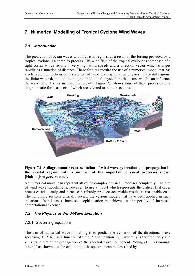
Queensland Government Queensland Climate Change and Community Vulnerability to Tropical CyclonesOcean Hazards Assessment - Stage 1
7. Numerical Modelling of Tropical Cyclone Wind Waves
7.1 Introduction
The prediction of ocean waves within coastal regions, as a result of the forcing provided by a tropical cyclone is a complex process. The wind field of the tropical cyclone is composed of a tight vortex which results in very high wind speeds and a direction vector which changes rapidly as a function of distance. These features require the use of a numerical model that hasa relatively comprehensive description of wind wave generation physics. In coastal regions, the finite water depth and the range of additional physical mechanisms, which can influence the wave field, further increase complexity. Figure 7.1 shows some of these processes in a diagrammatic form, aspects of which are referred to in later sections.
WindBreaking Quadruplets
Surf Breaking
Bottom Friction
Triads
Figure 7.1 A diagrammatic representation of wind wave generation and propagation in
the coastal region, with a number of the important physical processes shown
[Holthuijsen pers. comm.].
No numerical model can represent all of the complex physical processes completely. The aimof wind wave modelling is, however, to use a model which represents the critical first orderprocesses adequately and hence can reliably produce acceptable results at reasonable cost.The following sections critically review the various models that have been applied in suchsituations. In all cases, increased sophistication is achieved at the penalty of increased computational expense.
7.2 The Physics of Wind-Wave Evolution
7.2.1 Governing Equations
The aim of numerical wave modelling is to predict the evolution of the directional wave spectrum, ( , )F f , as a function of time, and position t ,x y , where f is the frequency and
is the direction of propagation of the spectral wave component. Young (1999) (amongst
others) has shown that the evolution of the spectrum can be described by
J0004-PR0001C 99 March 2001
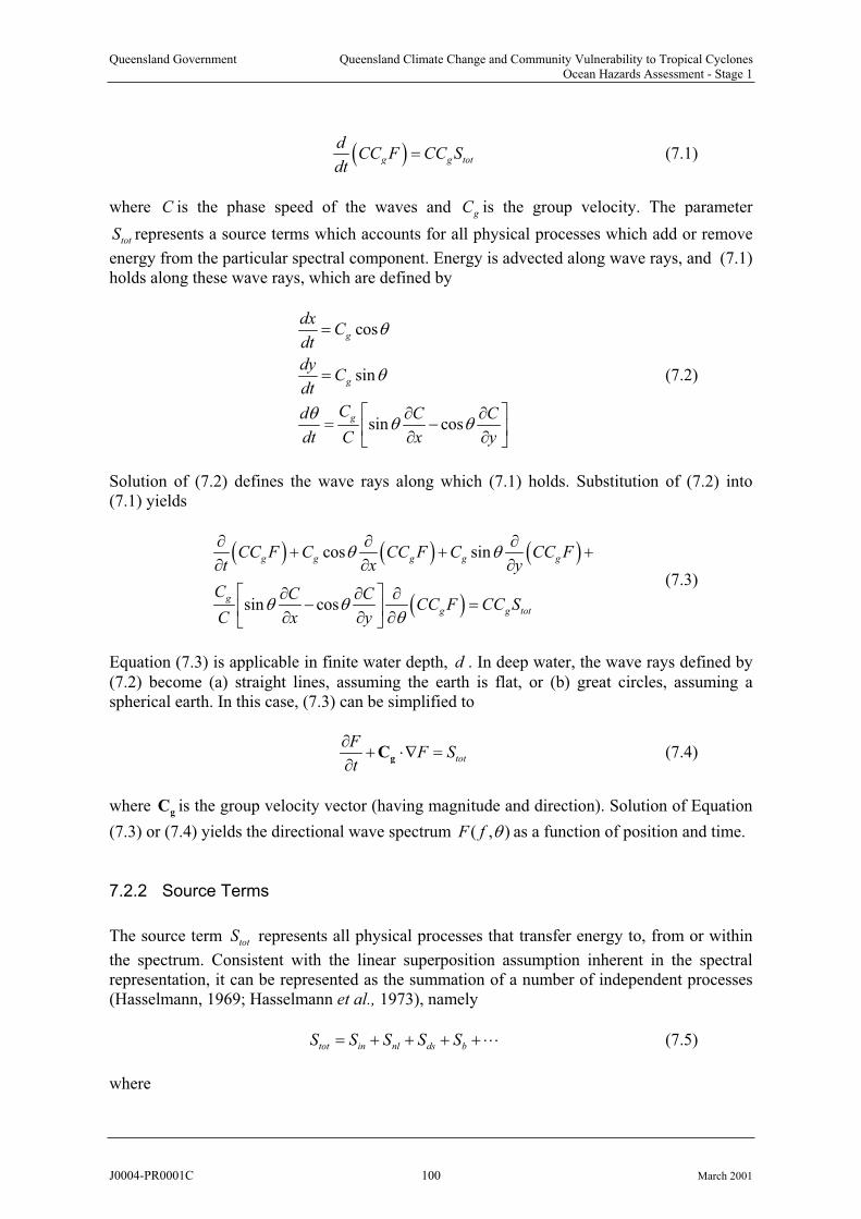
Queensland Government Queensland Climate Change and Community Vulnerability to Tropical CyclonesOcean Hazards Assessment - Stage 1
g g tot
dCC F CC S
dt (7.1)
where is the phase speed of the waves and C gC is the group velocity. The parameter
represents a source terms which accounts for all physical processes which add or remove
energy from the particular spectral component. Energy is advected along wave rays, and (7.1) holds along these wave rays, which are defined by
totS
cos
sin
sin cos
g
g
g
dxC
dt
dyC
dt
Cd C
dt C x y
C
(7.2)
Solution of (7.2) defines the wave rays along which (7.1) holds. Substitution of (7.2) into (7.1) yields
cos sin
sin cos
g g g g g
g
g g tot
CC F C CC F C CC Ft x y
C C CCC F CC S
C x y
(7.3)
Equation (7.3) is applicable in finite water depth, . In deep water, the wave rays defined by
(7.2) become (a) straight lines, assuming the earth is flat, or (b) great circles, assuming a spherical earth. In this case, (7.3) can be simplified to
d
tot
FF S
tgC (7.4)
where is the group velocity vector (having magnitude and direction). Solution of Equation
(7.3) or (7.4) yields the directional wave spectrum
gC
( , )F f as a function of position and time.
7.2.2 Source Terms
The source term represents all physical processes that transfer energy to, from or within
the spectrum. Consistent with the linear superposition assumption inherent in the spectral representation, it can be represented as the summation of a number of independent processes (Hasselmann, 1969; Hasselmann et al., 1973), namely
totS
(7.5) tot in nl ds bS S S S S
where
J0004-PR0001C 100 March 2001

Queensland Government Queensland Climate Change and Community Vulnerability to Tropical CyclonesOcean Hazards Assessment - Stage 1
inS atmospheric input from the wind
nlS nonlinear interactions between spectral components
dsS dissipation due to "white-capping"
bS dissipation due to interaction with the bottom
The four processes listed above are not exhaustive and there are undoubtedly many otherfactors that influence the evolution of waves. Knowledge in this area is far from complete.The processes listed above do, however, appear to account for the major fluxes of energy to the spectrum. The first three are all important in deep water, whilst interactions with thebottom are clearly only applicable in finite depth water. A detailed discussion of the functional forms for each of these source terms can be found in Young (1999).
7.3 Numerical Modelling of Waves
7.3.1 Introduction
A comprehensive model that incorporates our full understanding of wind wave physics and is applicable in all situations would be prohibitively expensive. Instead, a variety of models have been proposed for applications in specific situations. In order to select the most appropriate model requires an understanding of the relative importance of the various physical processesactive in each domain. Such a classification has been presented by Battjes (1994), a modified form of which appears in Table 7.1. The table divides wave prediction into four physicaldomains:
Deep Oceans - where bottom influences can be neglected.
Shelf Seas - area between the deep oceans and the shoaling zone.
Shoaling Zone - the area where shoaling becomes important.
Harbours - taken to represent areas where there is an interaction between the waves and any structure (e.g. breakwater, oil platform, island, reef, etc.).
Table 7.1 The relative importance of various physical mechanisms in different domains.
Physical Process Deep Oceans Shelf Seas Shoaling Zone Harbours
Diffraction
Depth refract./shoaling
Current refraction
4 wave interactions
3 wave interactions
Atmospheric input
White-capping
Depth breaking
Bottom friction
- negligible; - minor importance; - significant; - dominant [after Battjes (1994)].
Models can be divided into two general classes: phase resolving models, which predict boththe amplitude and phase of individual waves and phase averaging models which predict
average quantities such as the spectrum or its integral properties ( sH the significant wave
height, pf the spectral peak frequency, etc.). Should phase averaged properties vary rapidly
J0004-PR0001C 101 March 2001

Queensland Government Queensland Climate Change and Community Vulnerability to Tropical CyclonesOcean Hazards Assessment - Stage 1
(order of a few wavelengths) then it will generally be necessary to use a phase resolving model. Conversely, should the wave properties vary slowly, on a scale of many wavelengths, then phase averaging models should be adopted.
Neither of the two general classes is superior, their domains of application often do not overlap. Nevertheless, Battjes (1994) concludes that: "Phase resolving models are
computationally so much more demanding (per unit area of computational domain) that they should be used only where they are strictly needed". Of the processes considered in Table 7.1 only diffraction and 3 wave nonlinear interactions require phase resolving models. Hence, the domain of application of phase resolving models is generally confined to wave-structure interactions (harbours etc.) and the nearshore zone, where 3 wave interactions becomeimportant. Even around coastal islands and reefs there is little evidence that diffraction is important. Recent spectral models have also included 3 wave interactions in an approximateform (Eldeberky and Battjes, 1995). In the context of tropical cyclone wave prediction, even in the coastal environment, spectral (phase averaging) models have been shown to produce reliable results and the remainder of this review will be limited to this type of model.
7.3.2 Source Term Representation
The sophistication with which the source term has been represented has largely paralleled
the increasing understanding of the physical processes responsible for wind-wave evolution and the exponential increase in available computational resources. Models are typically classed as first, second or third generation. These classifications are briefly described in Table7.2.
totS
Table 7.2 Definition of model classes based on the representation of the source terms.
inS nlS dsS
First Generation Based on growthrate measurements
Large in magnitude
Saturation limit
Second Generation Based on fluxmeasurements
Smaller than 1st
Generation
Parametric form
Limited flexibility
Saturation limit, as in 1st Generation
Third Generation Based on fluxmeasurements
Stress coupled tosea state
Approximate formof Boltzmanintegral
Explicit form
Each of these classes of model is discussed in the following sections.
7.3.3 First Generation Models
The first attempt to develop a wave prediction model based on a numerical solution to (7.4) was made by Gelci et al. (1957). This model pre-dated the development of the theory of quadruplet nonlinear interactions by Hasselmann (1962) and the source term was considered to be the sum of atmospheric input and white-cap dissipation.
(7.6) (1) (1) (1)
tot in dsS S S
Models of this type are termed first generation, as indicated by the superscripts in (7.6). Anumber of other first generation models were later based on this same source term description
J0004-PR0001C 102 March 2001
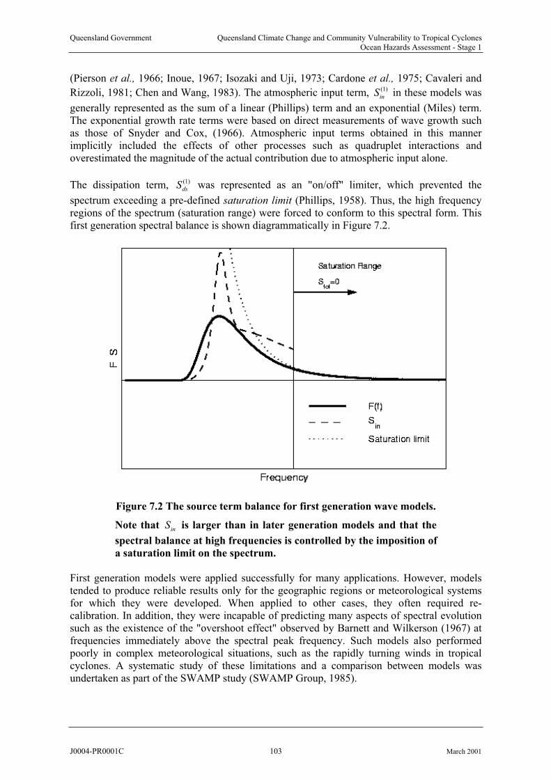
Queensland Government Queensland Climate Change and Community Vulnerability to Tropical CyclonesOcean Hazards Assessment - Stage 1
(Pierson et al., 1966; Inoue, 1967; Isozaki and Uji, 1973; Cardone et al., 1975; Cavaleri and
Rizzoli, 1981; Chen and Wang, 1983). The atmospheric input term, in these models was
generally represented as the sum of a linear (Phillips) term and an exponential (Miles) term.The exponential growth rate terms were based on direct measurements of wave growth such as those of Snyder and Cox, (1966). Atmospheric input terms obtained in this mannerimplicitly included the effects of other processes such as quadruplet interactions and overestimated the magnitude of the actual contribution due to atmospheric input alone.
(1)
inS
The dissipation term, was represented as an "on/off" limiter, which prevented the
spectrum exceeding a pre-defined saturation limit (Phillips, 1958). Thus, the high frequency regions of the spectrum (saturation range) were forced to conform to this spectral form. This first generation spectral balance is shown diagrammatically in Figure 7.2.
(1)
dsS
Figure 7.2 The source term balance for first generation wave models.
Note that is larger than in later generation models and that the
spectral balance at high frequencies is controlled by the imposition of
a saturation limit on the spectrum.
inS
First generation models were applied successfully for many applications. However, modelstended to produce reliable results only for the geographic regions or meteorological systemsfor which they were developed. When applied to other cases, they often required re-calibration. In addition, they were incapable of predicting many aspects of spectral evolutionsuch as the existence of the "overshoot effect" observed by Barnett and Wilkerson (1967) at frequencies immediately above the spectral peak frequency. Such models also performedpoorly in complex meteorological situations, such as the rapidly turning winds in tropical cyclones. A systematic study of these limitations and a comparison between models was undertaken as part of the SWAMP study (SWAMP Group, 1985).
J0004-PR0001C 103 March 2001
Queensland Government Queensland Climate Change and Community Vulnerability to Tropical CyclonesOcean Hazards Assessment - Stage 1
7.3.4 Second Generation Models
The JONSWAP study (Hasselmann et al., 1973) clearly showed the central role played by quadruplet nonlinear interactions in the source term balance. Hence, it became clear that this
term must be included within operational models. A major impediment to the inclusion of ,
was the significant computational time required for its evaluation. In order to overcome this problem a class of wave models which utilized approximations to this term developed (Barnett, 1968; Ewing, 1971; Golding, 1983; Allender et al., 1985, Greenwood et al., 1985; Sobey and Young, 1986; Young, 1988a). This class of model, the source term balance ofwhich is shown in (7.7) become known as second generation models.
nlS
(7.7) (2) (2) (2) (2)
tot in nl dsS S S S
In contrast to first generation models, the atmospheric input term, was based on direct
measurements of the normal stress exerted on the water surface (Snyder et al., 1981). Hence, this term was significantly smaller than in first generation models. Also, many of the second generation models neglected the linear or Phillips term, as it was very small in comparison to the Miles exponential mechanism. The linear mechanism does, however, play a role in the initial growth of the spectrum from a calm sea. This initial "trigger" for growth was includedin these models by defining the initial conditions for the model as some small, but finite, spectral energy.
(2)
inS
The dissipation term was included as a saturation limit to the spectrum. As the results of
JONSWAP showed that this level varied with the wave age, a number of models included variable levels for this saturation spectrum.
(2)
dsS
The significant advancement with this class of model was the inclusion of a parametric
representation for the quadruplet nonlinear interaction term, . A number of
representations were implemented. In almost all cases these approximate forms representedthe model spectrum in terms of a small number (3 to 5) of parameters. The JONSWAPspectral parameters were a common choice (Barnett, 1968; Ewing, 1971; Young, 1988a).
As could be pre-computed for spectra with a range of these standard parameters, model
values of could then be determined based on the model spectral parameters. Naturally,
problems occurred when the model spectrum did not conform to any of those for which
had been precomputed. A further sub-class of models, termed hybrid models, took this process one step further and predicted the evolution of the parameters rather than the discretevalues of the two-dimensional directional spectrum. Notable examples of these hybrid modelsare GONO (Sanders, 1976) and HYPA (Gunther et al., 1979).
(2)
nlS
nlS(2)
nlS
nlS
A diagrammatic representation of the source terms in second generation models is shown in Figure 7.3. In contrast to first generation models [Figure 7.2], it is clear that the inclusion of the nonlinear term has resulted in a reduction in the magnitude of the atmospheric input.
The inclusion of the parametric representations for generally resulted in an enhanced
modelling capability. Even in demanding situations such as tropical cyclone wind fields, second generation models were able to produce reasonable results (Young, 1988a). Despite this, the relatively simple formulation for the nonlinear source term represented a significantshort-coming of these models.
nlS
J0004-PR0001C 104 March 2001
Queensland Government Queensland Climate Change and Community Vulnerability to Tropical CyclonesOcean Hazards Assessment - Stage 1
Figure 7.3 The source term balance for second generation wave models.
Note that is smaller than in first generation models [see Figure 7.2]. inS
7.3.5 Third Generation Models
By the middle 1980s a multitude of 1st and 2nd generation models were operational. Many of these were used for commercial purposes and numerous claims were made about the benefits of one model as opposed to another. In order to compare the physics of the various modelsand to assess their strengths and weaknesses a major international intercomparison study was initiated - the Sea Wave Modeling Project, SWAMP, (SWAMP Group, 1985). Rather than compare models against field data, this study utilized a series of idealized test cases, designed to highlight specific aspects of model physics. One of the significant findings of the study was: "All present second-generation models suffer from limitations in the parameterization of
the nonlinear energy transfer, S ". The directional wave spectrumnl ( , )F f is typically
represented by discrete values. In order to define the two-dimensional frequency-direction space, of order 100 points are required (typical implementations use about 300 values). The
parameterizations for S typically use a maximum of 5 parameters. The mismatch is
obvious: How can the evolution of a spectrum with hundreds of degrees of freedom bedescribed by a source term defined by only a handful of parameters?
(2)
nl
The solution to these short-comings was, however, a significant problem and the first steps to a solution were made in the spring of 1984 when Klaus Hasselmann invited wave researchers to Hamburg to discuss the possibility of a joint endeavour. The WAM (WAve Modelling)Group was formed. The aim of the group was to develop a third generation model, free from many of the assumptions that constrained earlier generation models. This significant international collaboration resulted in the WAM Model (WAMDI, 1988). Variants of this basic model were also developed by Tolman (1991) (WAVEWATCH) and more recently by Booij et al. (1996) (SWAN).
J0004-PR0001C 105 March 2001

Queensland Government Queensland Climate Change and Community Vulnerability to Tropical CyclonesOcean Hazards Assessment - Stage 1
The source term balance in third generation models is essentially the same as in second generation models, that is
(7.8) (3) (3) (3) (3)
tot in nl dsS S S S
The details of the source terms are, however, significantly different to second generation
models. The early versions of the WAM model utilized the Snyder et al. (1981) form of as
in second generation models. Later versions, however, incorporated the coupled air water drag model of Janssen (1991). In principal, a third generation model should have a full solution to the nonlinear quadruplet interaction term. In practice, however, this is still notcomputationally feasible in a two-dimensional model. Third generation models utilize thediscrete interaction approximation (DIA) to the term (Hasselmann et al., 1985). Although the
DIA is still an approximation to , it is very different in its formulation to the simple
parametric forms used in second generation models. The DIA retains the basic physics of the nonlinear interaction process, but considers a very small sub-set of all the possible
interactions. In contrast to second generation parameterizations for , which have only a few
degrees of freedom, the DIA has as many degrees of freedom as there are values in thediscretely specified directional spectrum,
inS
nlS
nlS
( , )F f .
As both the input and nonlinear terms of second generation models had significantly fewerdegrees of freedom than the spectrum, the only way that stable spectral evolution could be achieved was by imposing the saturation limit at high frequencies. This is not necessary with third generation models and explicit forms for the still poorly understood white-cap
dissipation term, , can be utilized. The general form used has been that of Komen et al.
(1984).
dsS
The form of the source terms utilized in third generation models is shown in Figure 7.4. The significant difference compared to second generation models is that no artificially defined saturation limit is required to maintain a spectral balance at high frequencies. The spectrum is allowed to evolve without constraint until, at high frequencies a balance is achieved
where .(3) 0totS
7.4 Computational Aspects
In addition to defining the source terms there are a number of computational aspects whichneed to be considered in the development of any numerical model. These include the advection scheme to be used, the specification of the computational grid and the initial andboundary conditions. Many of these aspects are common to the solution of advective transport equations found in related areas of computational physics and the model designer can drawextensively from this literature. There are, however, some unique problems associated with wave prediction which require specific attention. The vast bulk of the international wavemodelling effort has been concentrated on the specification of the source terms. In comparison, the numerical aspects have received minimal attention.
J0004-PR0001C 106 March 2001
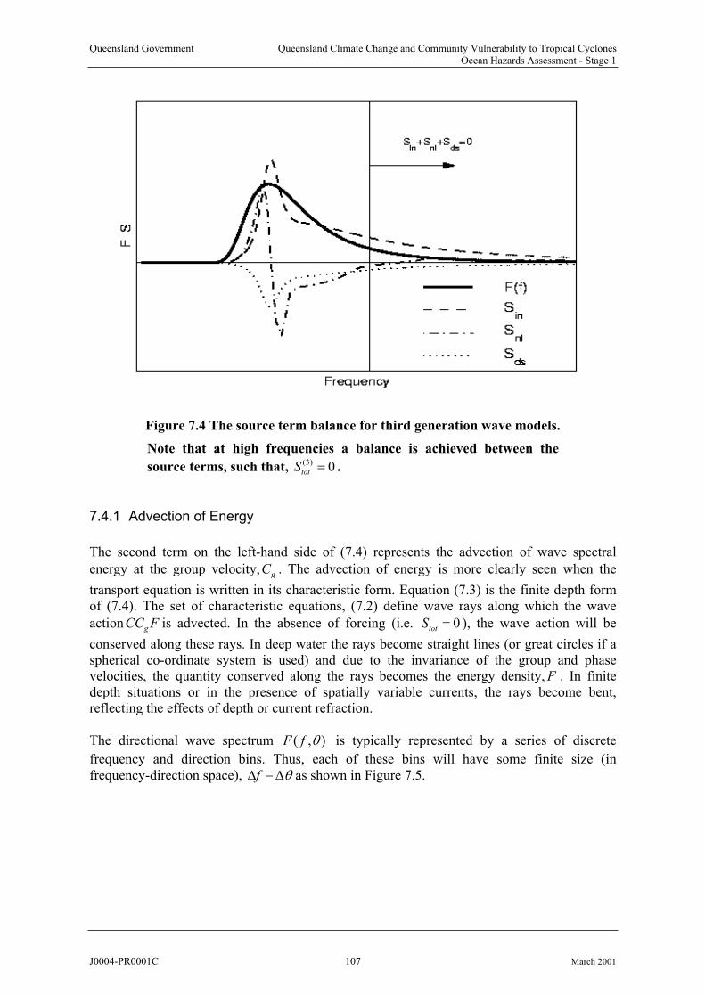
Queensland Government Queensland Climate Change and Community Vulnerability to Tropical CyclonesOcean Hazards Assessment - Stage 1
Figure 7.4 The source term balance for third generation wave models.
Note that at high frequencies a balance is achieved between the
source terms, such that,(3) 0totS .
7.4.1 Advection of Energy
The second term on the left-hand side of (7.4) represents the advection of wave spectral
energy at the group velocity, gC . The advection of energy is more clearly seen when the
transport equation is written in its characteristic form. Equation (7.3) is the finite depth formof (7.4). The set of characteristic equations, (7.2) define wave rays along which the wave
actionCC is advected. In the absence of forcing (i.e.g F 0totS ), the wave action will be
conserved along these rays. In deep water the rays become straight lines (or great circles if a spherical co-ordinate system is used) and due to the invariance of the group and phase velocities, the quantity conserved along the rays becomes the energy density, . In finitedepth situations or in the presence of spatially variable currents, the rays become bent,reflecting the effects of depth or current refraction.
F
The directional wave spectrum ( , )F f is typically represented by a series of discrete
frequency and direction bins. Thus, each of these bins will have some finite size (infrequency-direction space), f as shown in Figure 7.5.
J0004-PR0001C 107 March 2001
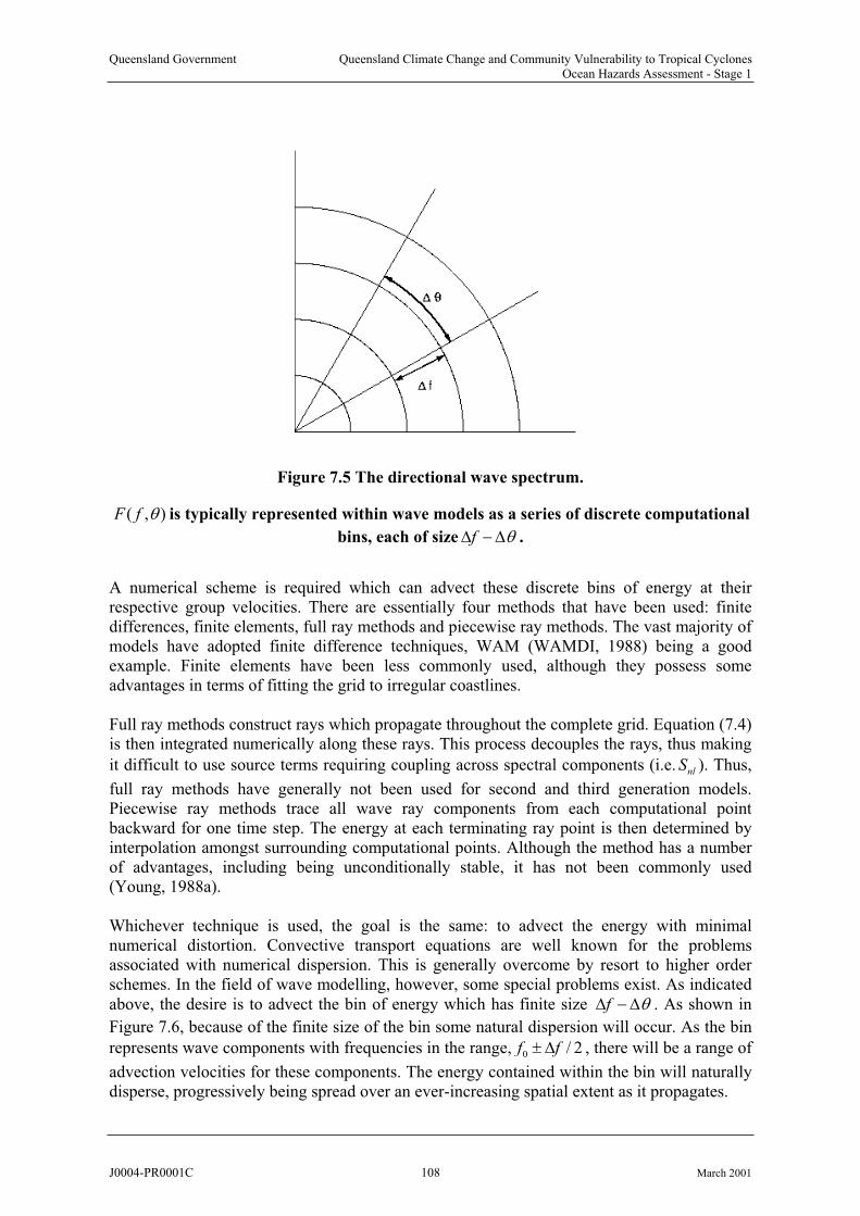
Queensland Government Queensland Climate Change and Community Vulnerability to Tropical CyclonesOcean Hazards Assessment - Stage 1
Figure 7.5 The directional wave spectrum.
( , )F f is typically represented within wave models as a series of discrete computational
bins, each of size f .
A numerical scheme is required which can advect these discrete bins of energy at their respective group velocities. There are essentially four methods that have been used: finite differences, finite elements, full ray methods and piecewise ray methods. The vast majority of models have adopted finite difference techniques, WAM (WAMDI, 1988) being a good example. Finite elements have been less commonly used, although they possess someadvantages in terms of fitting the grid to irregular coastlines.
Full ray methods construct rays which propagate throughout the complete grid. Equation (7.4) is then integrated numerically along these rays. This process decouples the rays, thus making
it difficult to use source terms requiring coupling across spectral components (i.e. ). Thus,
full ray methods have generally not been used for second and third generation models.Piecewise ray methods trace all wave ray components from each computational pointbackward for one time step. The energy at each terminating ray point is then determined byinterpolation amongst surrounding computational points. Although the method has a numberof advantages, including being unconditionally stable, it has not been commonly used (Young, 1988a).
nlS
Whichever technique is used, the goal is the same: to advect the energy with minimalnumerical distortion. Convective transport equations are well known for the problemsassociated with numerical dispersion. This is generally overcome by resort to higher order schemes. In the field of wave modelling, however, some special problems exist. As indicated above, the desire is to advect the bin of energy which has finite size f . As shown in
Figure 7.6, because of the finite size of the bin some natural dispersion will occur. As the bin
represents wave components with frequencies in the range, 0 / 2f f , there will be a range of
advection velocities for these components. The energy contained within the bin will naturallydisperse, progressively being spread over an ever-increasing spatial extent as it propagates.
J0004-PR0001C 108 March 2001

Queensland Government Queensland Climate Change and Community Vulnerability to Tropical CyclonesOcean Hazards Assessment - Stage 1
Figure 7.6 The natural dispersion of the bin of energy as it is advected.
Due to the finite range of group velocities and propagation directions
contained within the bin, the spatial extent of the bin will increase
with time. The single dots at the centre of the bin show the result of
the use of a propagation scheme that has no numerical dispersion.
As shown in Figure 7.6, spatial extent of the bin of energy increases linearly with time. A consistent numerical propagation scheme should reproduce these linear dispersion rates.Figure 7.6 also shows the spatial distribution resulting from a propagation scheme with no dispersion. The energy will be concentrated at a single point at the centre of the continuallyenlarging bin of energy. The resulting "spotty" distribution of energy has been termed the garden sprinkler effect. Booij and Holthuijsen (1987) have shown that the required linear spreading rates may be achieved by introducing a variable diffusion coefficient proportional to the age of the bin of energy. To date, this concept has not been tested in the context of a fullmodel.
As a result of the garden sprinkler effect, use of higher order propagation schemes will not necessarily improve results. To date, operational models have generally used relatively low order propagation schemes in the hope that the numerically dispersion inherent in such schemes is not too dissimilar to the required natural dispersion. As an example, the WAMmodel uses a first order upwinding scheme. In justification for this choice Janssen et al.
(1994) take the pragmatic stance: "... we have chosen the first order upwinding scheme
because it is the simplest scheme to implement (requiring less computer time and memory)and because in practice it gives reasonable results". Higher order schemes have, however, been reported to yield improved results: Tolman (1992) - second order and Bender, (1996) - third order.
It is clear from the discussion above that relatively little effort has been devoted to the propagation algorithms used in present-day wave prediction models. Although it is claimedthat present day models, such as WAM, predict swell propagation to a reasonable level ofprecision, other influences may also be active. The white-cap dissipation terms in thirdgeneration models have been "tuned" to ensure growth rates of wind sea and decay rates of
J0004-PR0001C 109 March 2001

Queensland Government Queensland Climate Change and Community Vulnerability to Tropical CyclonesOcean Hazards Assessment - Stage 1
swell agree with measurements. Hence, the apparently acceptable results may be a result of this artificial tuning. It is reasonable to conclude that further research into the development of appropriate propagation algorithms for use in wind-wave models is required.
7.4.2 Computational Grids
Equation 7.4 must be solved on a two-dimensional spatial grid. The precise details of this computational grid can have significant influence on the solution. The grid must be sufficiently fine to ensure that the spatial distribution of the wind field is adequately resolved.An often-conflicting requirement is that the extent of the model should remaincomputationally tractable. Often, conflicts of scale also occur. For instance, a goal may be to model the waves generated by an extreme tropical cyclone. Adequate resolution of the tight vortex wind field of a small-scale tropical cyclone may require a very fine resolution grid (e.g.
km). At the same time, swell generated in this intense wind region can propagate large
distances. Thus the spatial extent of the grid may need to be large (e.g. 2,000 km). Similarly,an extremely fine resolution grid may be required to accurately define the bathymetry in a coastal area. The meteorological system which generated the swell entering this region may,however, have occurred many thousands of kilometres away.
5x <
These conflicts of scale are often accommodated by the use of nested grids, particularly for coastal applications. A relatively coarse grid is initially used to model the generation ofdistant waves. Any number of finer nested grids can then be successively embedded withinthis coarse grid. Each of these finer grids takes their respective boundary conditions from the coarser grid in which they are nested.
Numerical wave prediction models can be divided into two general classes: global scale models and regional models. Global models operate on spherical grids. A typical example isthe global WAM model which runs operationally at many centres, the most long standing implementation being that at the European Centre for Medium Range Weather Forecasting
(ECMWF). In its original implementation at ECMWF, WAM operated on a3 grid with a time
step of 20 minutes, the spectral grid being represented by 25 frequencies and 12 directions. In
later versions of the model, the spatial resolution was increased to1.5 .
0
0
At the other extreme, regional models often operate on Cartesian grids with resolutions as fineas a few hundred metres. Although the resolution can be reduced further, some consideration of the rationale for such a grid is required. Phase averaging models assume that the spectrumis changing relatively slowly, compared with the wave length. Therefore, if it is expected that the wave field will change significantly over a length of order 10 wave lengths, than thevalidity of the phase averaged model is questionable.
In addition to the selection of appropriate spatial resolution, the time step also needs to bematched to the particular problem. In models that use explicit finite difference schemes, such as WAM, the upper bound on the time step t is specified by the requirements of numerical
stability. The Courant limit requires / gt x C< , where x is the spatial resolution. Hence,
the energy is constrained to propagate, at most, one grid element during the time step. At firstappearances this may seem an overly restrictive limitation and the use of implicit schemesmay seen advantageous. Such schemes may remain numerically stable with larger time stepsbut they are not necessarily accurate. If the spatial scale has been chosen to resolve thebathymetry and wind forcing, the time step should be such that wave energy propagating
J0004-PR0001C 110 March 2001

Queensland Government Queensland Climate Change and Community Vulnerability to Tropical CyclonesOcean Hazards Assessment - Stage 1
through the area can appropriately interact with the local source terms. Hence, the Courant limit seems an appropriate upper bound for the time step to ensure, not only numericalstability, but also accuracy of the numerical solution.
7.4.3 Initial and Boundary Conditions
Models that do not have a Phillips mechanism require some initial spectral energy level toinitiate growth. This is usually achieved by the introduction of a "seed" spectrum which has very low energy. The model then goes through a "spin-up" period where a wind field is imposed whilst the waves gradually reach a realistic level. The exact details of the seedspectrum are not important. One of the characteristics of spectral wave models (especiallythird generation models) is that they quickly modify the sea state to be in equilibrium with thelocal forcing wind.
All models require the specification of boundary conditions. Land boundaries are typically taken as completely absorbing with all energy being dissipated. Unless a global model is used, open boundary conditions must also be imposed. A common choice in such circumstances is to impose radiation conditions, in which energy can leave the computational domain but none can enter. If such boundaries are used, it is necessary to ensure that the computational domainis sufficiently large to ensure the boundary conditions do not influence the wave field at thepoints of interest.
7.5 The Tropical Cyclone Wave Field
Our present understanding of the tropical cyclone wave field has been gained from acombination of in situ measurements (both non-directional and directional) at single points during the passage of tropical cyclones, remote sensing data and the application of numericalmodels. Naturally, the wave field is strongly related to the driving wind field, which is usually
characterized by the velocity of forward movement,V , the maximum wind velocity in the
storm,V and the radius to maximum winds,
fm
max R ( e.g. refer Chapter 5).
Much of the tropical cyclone wave data collected using in situ instruments has been obtained for commercial purposes and consequently, only a small fraction is in the public domain. The first comprehensive attempt to collect data under tropical cyclone conditions was the Ocean Data Gathering Program (Shemdin, 1977). This program involved instruments on six offshore oil platforms in the Gulf of Mexico. These systems operated between 1968 and 1971, during which data were collected for four hurricanes, including Camille. The program has beendescribed in detail by Ward (1974) and Hamilton and Ward (1974).
Since 1972, the US NOAA Data Buoy Office has deployed buoys at various locations around the US coast (NOAA Data Buoy Office, 1973). Tropical cyclone data from these buoys have been presented in a number of publications including Withee and Johnson (1975).
In addition to the US data set, a significant tropical cyclone wave database has been established by the offshore oil industry on the northwest coast of Australia. Data have beenobtained from more than 25 tropical cyclones over a period in excess of 20 years (Harper etal., 1993).
J0004-PR0001C 111 March 2001
Queensland Government Queensland Climate Change and Community Vulnerability to Tropical CyclonesOcean Hazards Assessment - Stage 1
Although non-directional observations of tropical cyclone wave conditions are valuable, a more comprehensive understanding can be obtained from directional measurements.Directional spectral observations during the passage of tropical cyclones have been reported by Forristall et al. (1978) and Black (1979). Remotely sensed data using Synthetic Aperture
Radar data have also provided insight into the directional properties of waves within tropicalcyclones (Elachi et al., 1977; King and Shemdin, 1978; Shemdin, 1980; Gonzalez et al.,
1982; McLeish and Ross, 1983; Beal et al., 1986; Holt and Gonzalez, 1986).
Numerous models have been proposed for the prediction of waves within tropical cyclones. These range from the largely empirical (Bretschneider, 1959; Bretschneider, 1972; Ijima et
al., 1968; Ross, 1976; Young, 1988b) to those based on solution of the radiative transfer equation (Patterson, 1972; Bea, 1974; Uji, 1975; Cardone et al., 1977; Young 1988a).
Based on knowledge of the tropical cyclone wind field and the composite database of wave observations, a qualitative description of the tropical cyclone wave field emerges. The wind field is asymmetric, with higher winds to the left (Southern Hemisphere) of the tropical cyclone centre. The wave field has an even greater degree of asymmetry due to the combinedinfluence of the asymmetry of the wind field and the extended fetch that exists within a translating tropical cyclone. The wind vector in the intense wind region to the left of the stormcentre (Southern Hemisphere) is approximately aligned with the direction of forward propagation. Hence, waves generated in this region tend to move forward with the tropicalcyclone and therefore remain in high wind regions for an extended period of time [see Figure 7.7]. In contrast, waves generated on the low wind side of the storm (right side in Southern Hemisphere) propagate in the opposite direction to the tropical cyclone translation and rapidly move away from the high wind areas. Low frequency waves generated in the intense wind regions to the left of the storm centre will have group velocities which are typically greater
than the velocity of forward movement of the storm,V . Hence, these components will "out
run" the storm and appear as swell ahead of the storm centre. This swell radiates out from the spatially localized generation area. Hence, the spectrum ahead of the storm often consists of locally generated wind sea together with swell radiating from the centre of the storm. The two
wave systems often intersect at angles near . As they are significantly separated in both frequency and direction, they can co-exist without any significant non-linear interaction between the two systems.
fm
090
The concept of an "extended fetch" which occurs due to the forward motion of the storm is also important in determining the wave height within a tropical cyclone. Not only is the wave
height determined by the maximum wind speed,V , but also by the period of time the waves
remain within the intense wind region (Shemdin, 1977). AsV increases, the period of the
waves generated and hence the group velocity at which they propagate also increases.
Consequently,V must also increase for the most severe wave conditions to occur. Should the
tropical cyclone move too slowly, the waves will "outrun" the tropical cyclone, whereas should the tropical cyclone move too rapidly, the waves will be left behind. Consequently, for
a given value ofV , the wave height could be expected to increase with increasingV until a
maximum is reached. A further increase inV will result in a decrease in wave height.
Similarly, the spatial distribution of wave height (asymmetry) will also depend on
bothV andV .
max
fm
max
fm
fm
max fm
max
J0004-PR0001C 112 March 2001
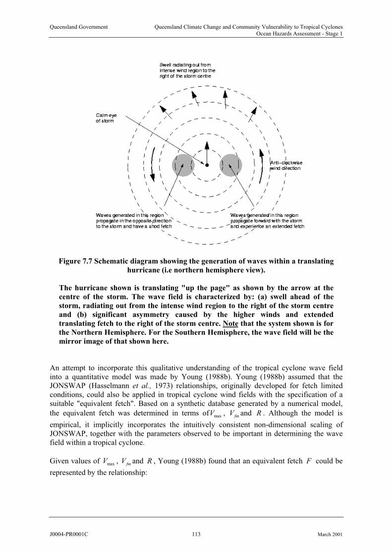
Queensland Government Queensland Climate Change and Community Vulnerability to Tropical CyclonesOcean Hazards Assessment - Stage 1
Figure 7.7 Schematic diagram showing the generation of waves within a translating
hurricane (i.e northern hemisphere view).
The hurricane shown is translating "up the page" as shown by the arrow at the
centre of the storm. The wave field is characterized by: (a) swell ahead of the
storm, radiating out from the intense wind region to the right of the storm centre
and (b) significant asymmetry caused by the higher winds and extended
translating fetch to the right of the storm centre. Note that the system shown is for
the Northern Hemisphere. For the Southern Hemisphere, the wave field will be the
mirror image of that shown here.
An attempt to incorporate this qualitative understanding of the tropical cyclone wave field into a quantitative model was made by Young (1988b). Young (1988b) assumed that theJONSWAP (Hasselmann et al., 1973) relationships, originally developed for fetch limitedconditions, could also be applied in tropical cyclone wind fields with the specification of a suitable "equivalent fetch". Based on a synthetic database generated by a numerical model,
the equivalent fetch was determined in terms ofV , andmax fmV R . Although the model is
empirical, it implicitly incorporates the intuitively consistent non-dimensional scaling of JONSWAP, together with the parameters observed to be important in determining the wave field within a tropical cyclone.
Given values of V , andmax fmV R , Young (1988b) found that an equivalent fetch could be
represented by the relationship:
F
J0004-PR0001C 113 March 2001

Queensland Government Queensland Climate Change and Community Vulnerability to Tropical CyclonesOcean Hazards Assessment - Stage 1
=F 2 2
max max maxfm fm fm
xaV bV V cV dV eV f
R (7.9)
where 32.175 10a ,b 21.506 10 , c 11.223 10 , , e12.190 10d 16.737 10
and . The term17.980 10f is a scaling factor which in the representation of Young
(1988b) was taken as 1. The term R can be found in terms of R as
(7.10) 322.5 10 log 70.8 10R R 3
In Equations (7.9) and (7.10) all terms are in standard S.I. units (i.e.V ,V - [m smax fm
-1];
,F R , R - [m]). The maximum significant wave height in the tropical cyclone, can then
be determined from a modified form of the JONSWAP (Hasselmann et al., 1973) relationship
ma
sH x
0.5max
2
max max
0.0016sgH gx
V V 2 (7.11)
The spatial distributions of sH are not obtainable directly in this case but have been
determined from a series of numerical experiments. sH can then be described in terms
using a series of diagrams for different values ofV and V .
max
sH
max fm
Examples of the predicted spatial distribution of sH
40
are shown in Figure 7.8. The spatial scale
is in terms of and the contours are of normalized significant wave height. In each case
the wave field has been normalized such that the maximum value is 1. In all cases the
maximum wind velocity in the storm,V
/r R
max m s-1. The velocity of forward movement
gradually increases in each panel: (a) V 2.5fm m s-1, (b) V 5.0fm m s-1, (c) V m s7.5fm
-1,
(d) V m s10.0fm
-1. The line of maximum winds max was chosen here as 70º (refer Chapter 5
for definitions). Note that all cases are shown for the Northern Hemisphere and SouthernHemisphere storms will the mirror images of those shown. For slow moving storms the
spatial distribution is similar to the wind speed distribution. As V increases the asymmetry
of the wave field increases significantly as both the asymmetry of the wind field and theextended fetch to the right (Northern Hemisphere) of the storm increases in significance. For
the largest values of V the region of maximum waves moves from the right forward quadrant
to the right rear quadrant. In these cases it is clear in the wave height distribution that thestorm is propagating so quickly that it is "out running" the waves.
fm
fm
The accuracy of the results of the approach proposed by Young (1988b) is limited by the fact that a numerical model generated the synthetic database used. To assess the applicability ofthis approach Young and Burchell (1996) compared the results of the model with
measurements of sH obtained from overflights of tropical cyclones by the GEOSAT satellite
altimeter. This satellite database was extensive, consisting of more than 100 tropical cyclones. Based on these data, Young and Burchell (1996) concluded that the model described by (7.9) contains a systematic bias and proposed that the scaling factor should take the form:
J0004-PR0001C 114 March 2001

Queensland Government Queensland Climate Change and Community Vulnerability to Tropical CyclonesOcean Hazards Assessment - Stage 1
Figure 7.8 The wave height distribution as predicted by the numerical model results of
Young (1988b).
max0.015 0.0431 1.30fmV V (7.12)
where againV andV have units of [m smax fm
-1] and is dimensionless. The resulting
distribution of equivalent fetch /x R obtained from (7.9) and (7.12) is shown in Figure 7.9.
The contours are of normalized equivalent fetch, /x R . The figure was generated from (7.9)
and (7.12). The surface takes the form of a ridge tilted towards the top right of the figure.
Therefore, as storms become more intense (increase in V ) they must move increasingly
more rapidly (larger values ofV ) to generate the maximum possible waves for that intensity
storm. Note that the relationships developed by Young and Burchell (1996) are not applicable outside the parameter range shown in this figure.
max
fm
J0004-PR0001C 115 March 2001
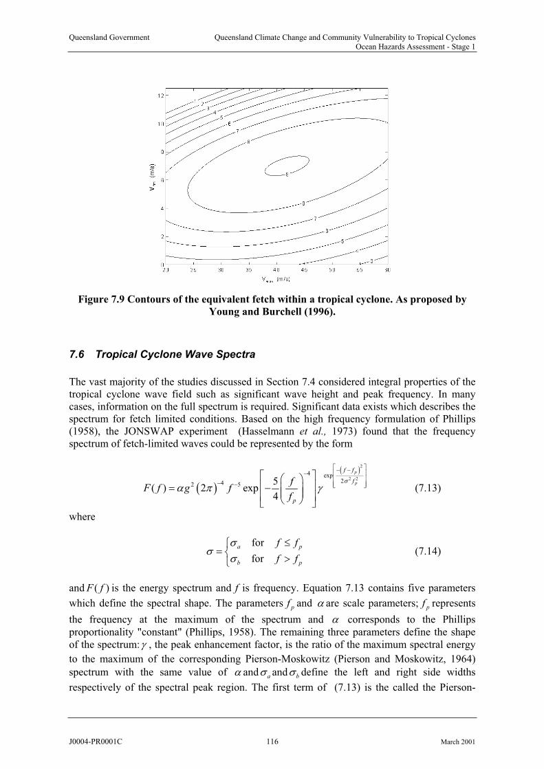
Queensland Government Queensland Climate Change and Community Vulnerability to Tropical CyclonesOcean Hazards Assessment - Stage 1
Figure 7.9 Contours of the equivalent fetch within a tropical cyclone. As proposed by
Young and Burchell (1996).
7.6 Tropical Cyclone Wave Spectra
The vast majority of the studies discussed in Section 7.4 considered integral properties of the tropical cyclone wave field such as significant wave height and peak frequency. In manycases, information on the full spectrum is required. Significant data exists which describes the spectrum for fetch limited conditions. Based on the high frequency formulation of Phillips (1958), the JONSWAP experiment (Hasselmann et al., 1973) found that the frequency spectrum of fetch-limited waves could be represented by the form
2
2 24 exp
242 5 5( ) 2 exp
4
p
p
f f
f
p
fF f g f
f (7.13)
where
for
for
a
b p
pf f
f f (7.14)
and is the energy spectrum and( )F f f is frequency. Equation 7.13 contains five parameters
which define the spectral shape. The parameters pf and are scale parameters; pf represents
the frequency at the maximum of the spectrum and corresponds to the Phillips
proportionality "constant" (Phillips, 1958). The remaining three parameters define the shape of the spectrum: , the peak enhancement factor, is the ratio of the maximum spectral energy
to the maximum of the corresponding Pierson-Moskowitz (Pierson and Moskowitz, 1964)
spectrum with the same value of and a and b define the left and right side widths
respectively of the spectral peak region. The first term of (7.13) is the called the Pierson-
J0004-PR0001C 116 March 2001
Queensland Government Queensland Climate Change and Community Vulnerability to Tropical CyclonesOcean Hazards Assessment - Stage 1
Moskowitz spectrum with the second term modifying the shape to make it more peaked. This
enhancement is only significant for pf f . At large / pf f the spectrum reverts to an 5f decay
as proposed by Phillips (1958).
4
p
f2 1f f
2.2
sH
fm
sH
An alternative formulation to (7.13), which has a high frequency region proportional
to 4f rather than 5f has been proposed by Donelan et al. (1985)
2
2 24 exp4
2( ) 2 expp
p
f f
fp dF f gf
(7.15)
Note that and d have been used here to distinguish from and in (7.13).
Studies that have considered detailed analysis of recorded wave spectra in tropical cyclonesare far rarer than corresponding studies of integral properties. Whalen and Ochi (1978) investigated the spectra recorded during the passage of U.S. Hurricanes Camille, Celia, Edith and Eloise. As with a number of previous observations, they found that as the tropical cyclone approached the recording site, the spectra were initially bi-modal. As the tropical cyclone moved closer, the spectra became uni-modal. They attempted to model the spectra using boththe JONSWAP form (Hasselmann et al., 1973) and the 6 parameter form proposed by Ochi and Hubble (1976). The Ochi and Hubble (1976) spectral form can represent bi-modal spectra and consequently, it provided a better fit to the data than JONSWAP for such spectra. TheJONSWAP spectrum, however, provided a good approximation to the data for the uni-modalspectra. They found that the data yielded mean JONSWAP parameters of and
0.023 . They also attempted to represent the parameters of the Ochi and Hubble (1976)
spectrum in terms of the significant wave height, . Although there appeared to be some
dependence on sH , there was significant scatter in the results. In view of the results of
Shemdin (1980), Young (1988b) and Young and Burchell (1996), which clearly demonstrate
that sH is a function of the relative position of the tropical cyclone, the velocity of forward
movement of the tropical cyclone,V and the maximum wind speed within the tropical
cyclone, V , it seems unlikely that a bi-modal spectral form could be parameterized in terms
of
max
sH , alone. The apparent dependence in the Whalen and Ochi (1978) data on is most
likely due to the very small number of tropical cyclones considered. Although there were four tropical cyclones in the total data base, the vast majority of the spectra were obtained fromHurricane Eloise.
Ochi and Chiu (1982) considered spectra recorded for U.S. Hurricane David. Again they confirmed that the JONSWAP form could model uni-modal spectra well and that the bi-modal spectra generated when the tropical cyclone was distant from the measurement site were well represented by the Ochi and Hubble (1976) form.
A detailed study of the properties of the one-dimensional spectrum, , under tropical
cyclone conditions was presented by Young (1997). Young (1997) considered data recorded over a 16 year period off the north-west coast of Australia. Spectra obtained from 16 tropicalcyclones were considered. The tropical cyclones had central pressures ranging from 905 hPa to 985 hPa. Hence, the data set was quite comprehensive. Young (1997) found that the spectra
( )F f
J0004-PR0001C 117 March 2001
Queensland Government Queensland Climate Change and Community Vulnerability to Tropical CyclonesOcean Hazards Assessment - Stage 1
were bi-modal when the storm centres were more than 8 times the radius to maximumwinds, R , from the measurement site. Spectra recorded within8R of the centre of the storm,
however, appeared similar to fetch limited spectra. This occurred despite the fact that the wind fields were changing rapidly in direction and that the wave field consisted of a mix of locally generated waves and distant swell. Young (1997) concluded that the shape stabilizing effects of the nonlinear source term were sufficient to continually force the spectra back to the uni-modal form. As the swell and wind sea components became more separated in frequencyand direction space (i.e. greater than8R from the storm centre), the nonlinear coupling
reduced in strength, and hence the spectra were bi-modal.
p
10
0.1
/ p
0.008
In order to assess whether the parametric spectral forms represented by JONSWAP (7.13) or Donelan et al. (1985) (7.14) may be suitable to model tropical cyclone spectra, Young (1997)
examined the exponent in the expression .n nF f
Figure 7.10 shows a scatter plot of n as a function of the inverse wave age,U C ,
whereC is the phase speed of components at the spectral peak frequency. There is significant
scatter in the data and no clear evidence that either of the proposed forms
10 / p
4f or 5f
4.56
is the
preferred form for the high frequency region of the spectrum. The mean value is ,
indicating either spectral form could be applied to the data. Such a result is consistent with thevariability of the exponent reported by Liu (1989) for fetch limited spectra.
n
n
Also shown in Figure 7.10 is the demarcation between wind-sea and swell, U C10 / 0.p 83
proposed by Donelan et al. (1985). Based on this limit, a significant proportion of the spectra
of this data set would normally be characterized as swell (i.e.U C/ 0.p 83 ). Despite this,
these spectra are still uni-modal.
7.6.1 JONSWAP Representation of Tropical Cyclone Spectra
As the spectral width parameter, , has little influence on the ultimate spectral form, and as
previous fetch limited studies had found no systematic trend within the scatter of values,Young (1997) assumed a constant value of this parameter of . Figures 7.11a and 7.11b
shown the values of and , respectively, for the JONSWAP form (7.13). Figure 7.11a also
shows the JONSWAP (Hasselmann et al., 1973) relationship for expressed in terms
ofU : 10 C
0.73
10
p
U
C (7.16)
Although there is significant scatter within the data, the values of clearly increase with
increasingU . The JONSWAP relationship (7.16), which was developed for fetch limited
waves, is a remarkably good fit to the data. This is a clear demonstration of the shape stabilization provided by non-linear interactions. Even though the wind fields from which these spectra were obtained are spatially and temporarily variable, the spectra are remarkablysimilar to those obtained from idealized fetch limited situations.
10 / pC
J0004-PR0001C 118 March 2001
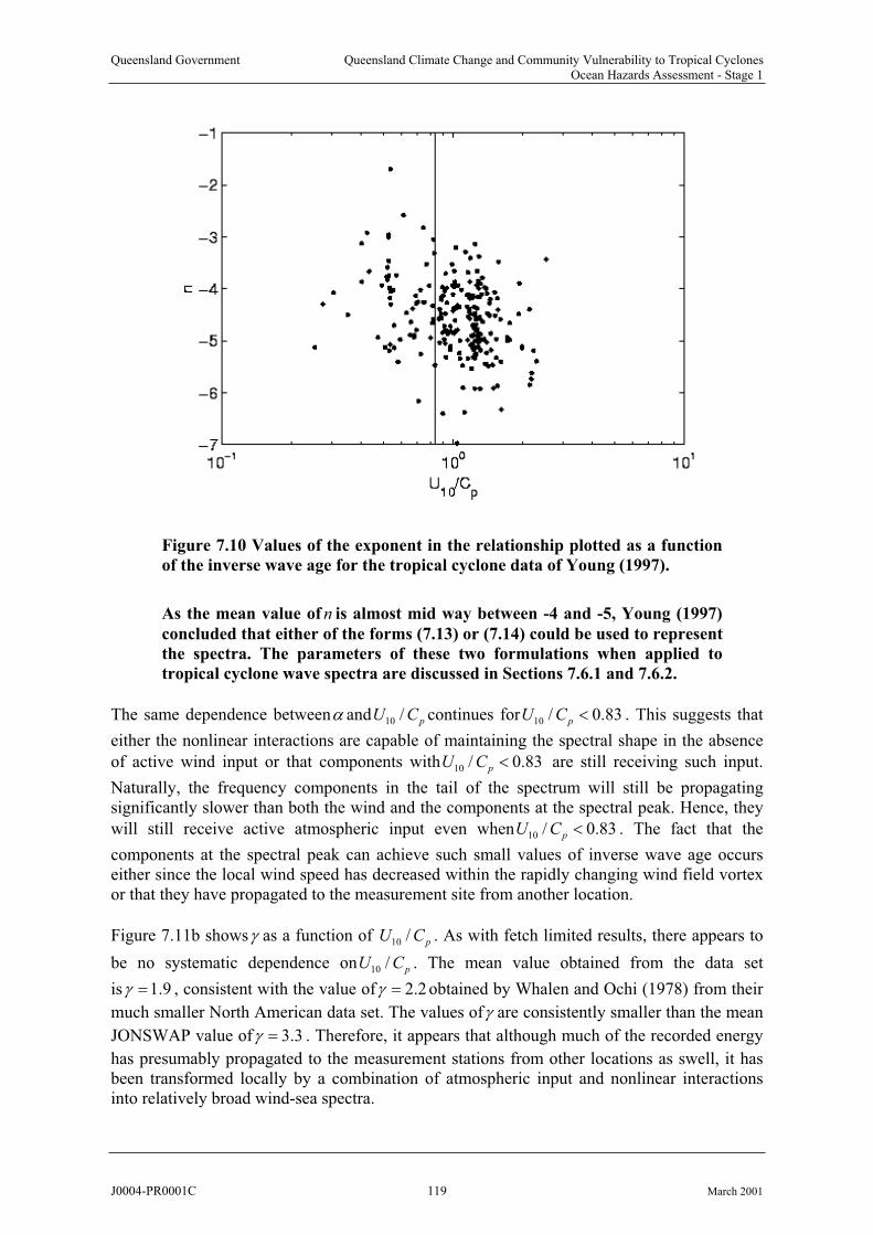
Queensland Government Queensland Climate Change and Community Vulnerability to Tropical CyclonesOcean Hazards Assessment - Stage 1
Figure 7.10 Values of the exponent in the relationship plotted as a function
of the inverse wave age for the tropical cyclone data of Young (1997).
As the mean value of n is almost mid way between -4 and -5, Young (1997)
concluded that either of the forms (7.13) or (7.14) could be used to represent
the spectra. The parameters of these two formulations when applied to
tropical cyclone wave spectra are discussed in Sections 7.6.1 and 7.6.2.
The same dependence between andU continues forU C10 / pC 10 / 0.p 83 . This suggests that
either the nonlinear interactions are capable of maintaining the spectral shape in the absence
of active wind input or that components withU C10 / p 0.83 are still receiving such input.
Naturally, the frequency components in the tail of the spectrum will still be propagatingsignificantly slower than both the wind and the components at the spectral peak. Hence, they
will still receive active atmospheric input even whenU C10 / 0.8p 3 . The fact that the
components at the spectral peak can achieve such small values of inverse wave age occurs either since the local wind speed has decreased within the rapidly changing wind field vortex or that they have propagated to the measurement site from another location.
Figure 7.11b shows as a function of U . As with fetch limited results, there appears to
be no systematic dependence onU . The mean value obtained from the data set
is
10 / pC
10 / pC
1.9 , consistent with the value of 2.2 obtained by Whalen and Ochi (1978) from their
much smaller North American data set. The values of are consistently smaller than the mean
JONSWAP value of 3.3 . Therefore, it appears that although much of the recorded energy
has presumably propagated to the measurement stations from other locations as swell, it hasbeen transformed locally by a combination of atmospheric input and nonlinear interactions into relatively broad wind-sea spectra.
J0004-PR0001C 119 March 2001
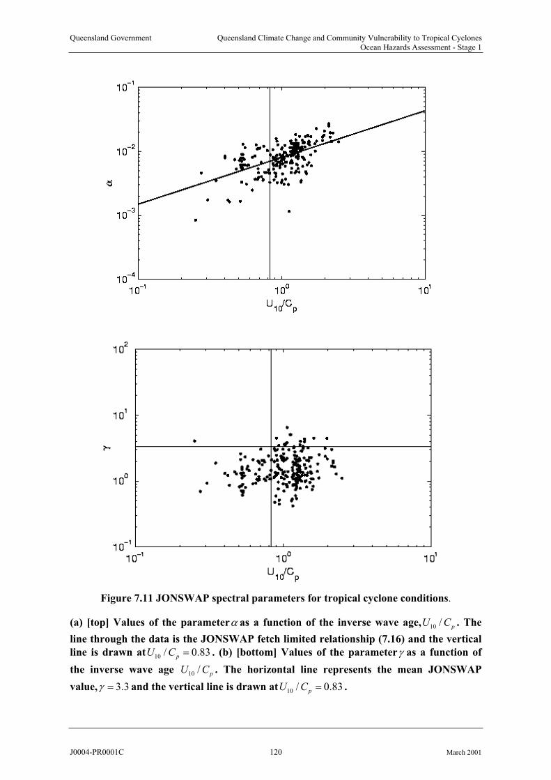
Queensland Government Queensland Climate Change and Community Vulnerability to Tropical CyclonesOcean Hazards Assessment - Stage 1
Figure 7.11 JONSWAP spectral parameters for tropical cyclone conditions.
(a) [top] Values of the parameter as a function of the inverse wave age,U . The
line through the data is the JONSWAP fetch limited relationship (7.16) and the vertical
line is drawn atU C b) [bottom] Values of the parameter
10 / pC
10 / 0.p .83 ( as a function of
the inverse wave age U . The horizontal line represents the mean JONSWAP
value,
10 / pC
3.3 and the vertical line is drawn atU C10 / 0.p 83 .
J0004-PR0001C 120 March 2001
Queensland Government Queensland Climate Change and Community Vulnerability to Tropical CyclonesOcean Hazards Assessment - Stage 1
7.6.2 Donelan et al. (1985) representation of Tropical Cyclone Spectra
Figures 7.12a and 7.12b show the parameters and d , respectively as functions ofU C ,
obtained for the Donelan et al. (1985) spectral form, Equation (7.15). The results are qualitatively similar to those shown in Figures 5.2 for the JONSWAP spectral form. Based ontheir fetch limited data, Donelan et al. (1985) proposed the following power law relationship
between
10 / p
andU .10 / pC
0.55
100.006p
U
C (7.17)
Equation (7.17) is shown in Figure 7.12a together with the present data. The relationshiprepresented by (7.17) is a remarkably good fit to the data, again indicating that the spectra are similar to fetch limited wind-sea spectra.
In contrast to JONSWAP (Hasselmann et al., 1973), Donelan et al. (1985) found a
dependence of d onU . They proposed the following functional form10 / pC
10
10 10 10
1.7 for 0.83 / 1
1.7 6.0 log / for 1.00 / 5
p
d
p p
U C
U C U C (7.18)
Equation (7.18) is shown in Figure 7.12b, together with the present data. There is significant
scatter in the values of d obtained from the tropical cyclone spectra and no clear trend is
apparent within this scatter. Equation (7.18) is, however, consistent with the data set,indicating the peak enhancement of the present data is comparable to that observed for fetch limited spectra.
The parametric representations of the data for both the JONSWAP and Donelan et al. (1985)forms yield the same general conclusions. Despite the complex temporally and spatiallyvariable wind fields of tropical cyclones, the spectra are remarkably similar to those measuredunder idealized fetch limited conditions. In addition, the spectra would generally be
characterized as mature wind-sea. The vast majority of the data are forU C . Indeed,
significant data are in the region, U C
10 / p 2
8310 / 0.p , which would normally be classified as
swell. The functional dependence of the spectral parameters for these values with
is, however, consistent with the more highly forced data. Hence, the processes
which force the spectra to conform to a parametric spectral form (such as nonlinearinteractions), apparently remain active in the absence of significant wind input at the spectral peak frequency.
10 / 0.pU C 83
J0004-PR0001C 121 March 2001

Queensland Government Queensland Climate Change and Community Vulnerability to Tropical CyclonesOcean Hazards Assessment - Stage 1
Figure 7.12 Donelan et al. (1985) spectral parameters for tropical cyclone conditions.
(a) [top] Values of the parameter as a function of the inverse wave age, U . The
line through the data is the Donelan et al. (1985) fetch limited relationship (7.17) and the
vertical line is drawn atU C he shaded region gives an estimate of the
magnitude of the 95% confidence limits on the individual data points. (b) [bottom]
Values of the parameter
10 / pC
10 .p .
d
/ 0 83 T
as a function of the inverse wave age, U . The line
through the data is the Donelan et al. (1985) fetch limited relationship (7.18) and the
vertical line is drawn at U C
10 / pC
10 / 0.p 83 . The shaded region gives an estimate of the
magnitude of the 95% confidence limits on the individual data points.
J0004-PR0001C 122 March 2001
Queensland Government Queensland Climate Change and Community Vulnerability to Tropical CyclonesOcean Hazards Assessment - Stage 1
7.7 Conclusions and Recommendations
The present application poses a number of considerable challenges for numerical wavemodelling. Tropical cyclone wind fields represent an intense wind vortex with the wind direction changing rapidly in space and time. The resulting wind seas are subjected toatmospheric input which also changes direction rapidly. This type of wind field is known to be a demanding test of model physics and generally requires the use of a sophisticated numerical model. In addition, coastal North Queensland is characterised by the presence of the Great Barrier Reef (GBR). The many reefs within the GBR, interspersed with narrow deep passages, will require very high resolution to adequately define the resulting bathymetry and potential for either local sheltering and/or wave transmission.
7.7.1 Choice of Model Physics
As described in Section 7.2, there are several choices of model physics which can be adopted. There are a number of examples of the successful use of 2nd Generation models under tropicalcyclone conditions (Young, 1988a). Generally, however, the rapidly changing direction of the wind field within such storms represents a very demanding test of such models. The
representation of in such models is generally based on the assumption that the spectrum
conforms well to a standard JONSWAP form and that swell wind-sea interaction is not significant. As shown in Section 7.4, spectra near the centre of the storm are, indeed, similar
to JONSWAP forms. This, however, is the result of the shape stabilization provided by . As
one moves further away from the storm centre, a point is eventually reached where swell andwind-sea can co-exist. In order to model both of these features successfully, requires the use
of a model with a sophisticated treatment of . These requirements mean that it is generally
highly desirable to adopt a 3
nlS
nlS
nlSrd Generation model under tropical cyclone conditions. If interest
is confined to the prediction of extreme conditions, as may occur near the centre of a landfalling tropical cyclone, a well tuned 2nd Generation model can produce acceptable results with considerably less computational expense. If this approach is adopted, it is important to select a model which has been extensively validated under extreme tropical cyclone conditions.
Waves generated by tropical cyclones can typically have periods as long as 13 seconds. Suchwaves will be modified by the typical water depths found on the continental shelf of Queensland. Hence the model adopted must be capable of representing depth dependent processes such as refraction and bottom friction. Although the water depth in the vicinity of coral reefs changes very rapidly (70 m to 0 m within 1 or 2 wavelengths), there is no observational evidence that diffraction is a significant mechanism in such areas. As a result, it is unlikely that time domain models are necessary in such situations.
The time-varying and directionally-changing nature of tropical cyclone forcing also prevents the practical application of commonly-used 2nd Generation coastal steady-state spectral wave models such as HISWA (Holthuijsen et al. 1989) and MIKE 20 (DHI 1991). These modelscan incorporate ambient current effects but the numerical solution methods limit wave propagation to within a narrow band relative to the orientation of the computational grid.
Based on the discussion above, there appears to be essentially three possible state-of-the-art model choices. These are WAM (Hasselmann et al., 1988), WAVEWATCH III (Tolman,1992) and SWAN (Booij et al., 1996). SWAN has the most refined finite depth physics of the
J0004-PR0001C 123 March 2001
Queensland Government Queensland Climate Change and Community Vulnerability to Tropical CyclonesOcean Hazards Assessment - Stage 1
three models and allows incorporation of the ambient current field, which could be significant in some storm tide situations. SWAN can also be used to estimate breaking wave setup (refer Chapter 8). SWAN is recommended for use in relatively small spatial domains (of the orderof 50 km) and earlier versions have a highly dispersive propagation scheme. As such, it should not be applied unilaterally for modelling tropical cyclone conditions unless nested incombination with a larger scale deepwater model which can provide adequate open boundary information. WAVEWATCH III has been developed from WAM, although the physics within the model has been changed to some degree and a more refined propagation scheme has been added (second order compared to first order in WAM). WAVEWATCH III is, however, adeep water model only and the present version does not have bottom friction implementedwithin the model. As a result, it also would not be suitable for unilateral application within theGreat Barrier Reef region. WAM, however, has the required 3rd Generation physics and is applicable within the transitional water depths of the Great Barrier Reef. A potential remaining drawback of WAM though is the relatively dispersive first order propagation scheme used in the original model. Because propagation distances for swell in the present situation are not great, this should not be a major problem. Adoption of a higher orderscheme, as described by Hardy et al. (2000), would however improve model performance in this regard.
It is recommended that a 3rd
Generation ocean wave model based on WAM (The WAMDI Group 1988) be used for the modelling program. If possible, the propagation scheme should
be updated, in a manner similar to that described by Hardy et al. (2000). For very fine scale
modelling the SWAN model (Booij et al. 1996) could be further nested within WAM to provide
optimal modelling in nearshore regions. If interest is confined to extreme conditions, near the
centre of the tropical cyclone, a 2nd
Generation model that has been extensively validated
under tropical cyclone conditions may also yield acceptable results. Ideally, some
comparative testing between a 3rd
Generation model and any proposed 2nd
Generation model
would indicate the suitability or otherwise of adopting a 2nd
Generation model.
7.7.2 Grid Considerations
The modelling of tropical cyclones represents a conflict of scales. It is necessary to use a computational grid which is sufficiently large to encompass swell generated by the tropicalcyclone when it is as far as 1000 km from the site of interest. At the same time, it is necessary to have a grid which is sufficiently fine to resolve the eye of the storm where the major wave generation regions are concentrated. The size of the eye varies, but may be as small as 20 km in diameter. In the present application, quite a fine grid will be required to adequately definethe many reefs within the GBR and the complex coastal bathymetry.
The requirements listed above dictate the use of nested grids, with finer scale grids takingtheir boundary conditions from coarser, larger scale grids. Young and Hardy (1993) and Hardy et al. (2000) have adopted this approach for the modelling of tropical cyclones within the GBR. Both studies have utilized a series of three grids. Hardy et al. (2000) adopted grid sizes of 37 km, 7.5 km and 1.5 km, respectively for the three grids used. The largest gridencompassed most of the Coral Sea. In addition, they adopted a sub-grid scale treatment of dissipation (blockage) by the scattered reefs of the area.
It is recommended that a grid system comparable to that of Hardy et al. (2000) and consistent
with other relevant scale parameters from Chapter 6 be adopted for any modelling in the
GBR region.
J0004-PR0001C 124 March 2001
Queensland Government Queensland Climate Change and Community Vulnerability to Tropical CyclonesOcean Hazards Assessment - Stage 1
A time step which is comparable with the spatial grid must also be adopted. If an explicit propagation scheme is adopted, the maximum time step is dictated by the Courant number (ie. energy can not propagate more than one grid square during the discrete time step). Implicitpropagation scheme allow larger time steps, whilst maintaining stability. Although such schemes may be stable with the adoption of larger time steps, there will be a loss of accuracy.If a grid of a specified size is required to adequately resolve the bathymetry, a time step
should be chosen such that / gt x C , where t and x are the model time and space steps,
respectively. This is effectively the same limit dictated by the Courant number. It may be possible to relax this limit for the larger scale grid, where resolution of the coastal bathymetryis not critical.
It is recommended that for the finer scale (B and C) grids, where practical, the time step be
chosen such that / gt x C .
7.7.3 Dissipation on Reefs
The scattered reefs of the GBR provide very effective dissipation of energy propagationthrough the region. Studies by Hardy and Young (1996) have shown, that even at high tide levels, considerable wave energy is dissipated by wave breaking and the high frictional resistance of the rough coral bottom. As a result, little energy is transmitted across individualreefs. As a result, Young and Hardy (1993) assumed that coral reefs acted effectively as land and dissipated all incident energy. This assumption produced acceptable results in their modelstudies. More recently, Hardy et al. (2000) have compared this assumption with a moreinvolved method where sub-grid scale reef blockage is accounted for by the use of a directional porosity factor for each grid point. They reported improved results using thisapproach.
It appears that the assumption of complete blockage produces acceptable results, provided the grid size is sufficiently small. Should sufficient resources be available, the approach of
Hardy et al. (2000) appears superior, both from a conceptual viewpoint and in terms of
reported performance.
7.8 References
Allender, J.H., Barnett, T.P. and Lybanon, M. (1985) The DNS model: An improved spectral model for ocean wave prediction. In: 'Ocean wave modeling', SWAMP Group, Plenum Press,New York, 235-248.
Barnett, T.P. (1968) On the generation, dissipation and prediction of ocean wind waves. J.
Geophys. Res., 73, 513-529.
Barnett, T.P. and Wilkerson, J.C. (1967) On the generation of ocean wind waves as inferredby airborne radar measurements of fetch-limited spectra. J. Marine Res., 25, 292-328.
Battjes, J.A. (1994) Shallow water wave modelling. Proc. Int. Symp.: Waves -- Physical and
Numerical Modelling, Vancouver, 1-23.
J0004-PR0001C 125 March 2001

Queensland Government Queensland Climate Change and Community Vulnerability to Tropical CyclonesOcean Hazards Assessment - Stage 1
Beal, R.C., Gerling, T.W., Irvine, D.E., Monaldo, F.M. and Tilley, D.G. (1986) Spatial variations of ocean wave directional spectra from the Seasat synthetic aperture radar. J.
Geophys. Res., 91, 2433-2449.
Bea, R.G. (1974) Gulf of Mexico hurricane wave heights. 6th Offshore Technology Conf.,Houston, OTC 2110.
Bender, L.C. (1996) Modification of the physics and numerics in a third-generation oceanwave model. J. Atmos. Oceanic Tech., 13, 726-750.
Black, J.L. (1979) Hurricane Eloise directional wave energy spectra. 11th Offshore
Technology Conf., Houston, OTC 3594.
Booij, N. and Holthuijsen, L.H. (1987) Propagation of ocean waves in discrete spectral wave models. J. Comp. Phys., 68, 307-326.
Booij, N., Holthuijsen, L.H. and Ris, R.C. (1996) The SWAN wave model for shallow water. Proc 25th Int. Conf. Coastal Eng., ASCE, Orlando, 668-676.
Bretschneider, C.L. (1959) Hurricane design - Wave practices. Trans. ASCE, 124, 39-62.
Bretschneider, C.L. (1972) A non-dimensional stationary hurricane wave model. 4th Offshore
Technology Conf., Houston, OTC 1517.
Cardone, V.J., Pierson, W.J. and Ward, E.G. (1975) Hindcasting the directional spectra of hurricane-generated waves. J. Pet. Technol., 261, 91-127.
Cardone, V.J., Ross, D.B. and Ahrens, M.R. (1977) An experiment in forecasting hurricane generated sea states. Proc. 11th Tech. Conf. on Hurricanes and Tropical Met., AMS, Miami.
Cavaleri, L. and Rizzoli, P.M. (1981) Wind wave prediction in shallow water: theory and application. J. Geophys. Res., 86, 10,961-10,973.
Chen, Y., and Wang, H. (1983) Numerical model of nonstationary shallow water wave spectral transformations. J. Geophys. Res., 88, 9851-9863.
DHI (1991) MIKE 20 nearshore module - user’s guide and reference manual, Danish
Hydraulic Institute.
Donelan, M.A., Hamilton, J. and Hui, W.H. (1985) Directional spectra of wind-generated waves. Philos. Trans. R. Soc. Lond., A 315, 509-562.
Elachi, C., Thompson, T.W., and King, D.B. (1977) Observations of the ocean wave patternunder Hurricane Gloria with Synthetic Aperture Radar. Science, 198, 609-610.
Eldeberky, Y. and Battjes, J.A. (1995) Parameterization of triad interactions in wave energymodels. Coastal Dynamics '95, Dally, W.R. and Zeidler, R.B. (eds), ASCE, 140-148.
Ewing, J.A. (1971) A numerical wave prediction method for the North Atlantic Ocean. Dtsch.
Hydrogh. Z., 24, 241-261.
J0004-PR0001C 126 March 2001
Queensland Government Queensland Climate Change and Community Vulnerability to Tropical CyclonesOcean Hazards Assessment - Stage 1
Forristall, G.Z., Ward, E.G., Cardone, V.J. and Borgmann, L.E. (1978) The directional spectra and kinematics of surface gravity waves in tropical storm Delia. Jnl. Phys. Oceangr., 8, 888-909.
Gelci, R., Cazale, J. and Vassal, J. (1957) Prevision de la houle. La methode des densites spectroangulaires. Bull. Inform. Comite Central Oceanogr. D'Etude Cotes, 9, 416-435.
Golding, B.W. (1983) A wave prediction system for real-time sea state forecasting. Q. J. Roy.Meteorol. Soc., 109, 393-416.
Gonzalez, F.I., Thompson, T.E., Brown, W.E. and Weissman, D.E. (1982) Seasat wind and wave observations of Northeast Pacific Hurricane Iva, August 13, 1978. J. Geophys. Res., 87, 3431-3438.
Greenwood, J.A., Cardone, V.J. and Lawson, L.M. (1985) Intercomparison test version of the SAIL wave model. In: 'Ocean wave modeling', SWAMP Group, Plenum Press, New York, 221-233.
Gunther, H., Rosenthal, W., Weare, T,J., Worthington, B.A., Hasselmann, K. and Ewing, J.A.(1979) A hybrid parametric wave prediction model. J. Geophys. Res., 84, 5727-5738.
Hamilton, R.C., and Ward, W.G. (1974) Ocean data gathering program - quality andreduction of data. 6th Offshore Technology Conf., Houston, OTC 2108-A.
Hardy, T.A., Mason, L.B. and McConochie, J.D. (2000) A wave model for the Great Barrier Reef. Ocean Engineering, (in press).
Hardy, T.A. and Young, I.R. (1996) Field study of wave attenuation on an offshore coral reef. J. Geophys. Res., 101, 14,311-14,326.
Harper, B.A., Mason, L.B., and Bode, L. (1993) Tropical cyclone Orson - a severe test for modelling. Proc. 11th Aust. Conf. Coastal and Ocean Eng., IEAust, Townsville, 59-64.
Hasselmann, K. (1962) On the non-linear energy transfer in a gravity-wave spectrum, Part 1. General Theory. J. Fluid Mech., 12, 481-500.
Hasselmann, K. (1969) Weak-interaction theory of ocean waves. Basic Developments in Fluid
Mech., 2, 117-182.
Hasselmann, K. et al. (1973) Measurements of wind-wave growth and swell decay during the Joint North Sea Wave Project (JONSWAP). Suppl. A, 8, 12, 95pp.
Hasselmann, S. and Hasselmann, K. (1985) The wave model EXACT-NL. In 'Ocean wave modelling' (The SWAMP Group), 249-251, New York, Plenum Press.
Holt, B., and Gonzalez, F.I. (1986) SIR-B Observations of dominant ocean waves near Hurricane Josephine. J. Geophys. Res., 91, 8595-8598.
J0004-PR0001C 127 March 2001
Queensland Government Queensland Climate Change and Community Vulnerability to Tropical CyclonesOcean Hazards Assessment - Stage 1
Holthuijsen, L.H., Booij, N. and Herbers, T.H.C. (1989), A prediction model for stationary, short-crested waves in shallow water with ambient currents, Coastal Engineering, 13, pp 23-54.
Ijima, T., Soejima, T. and Matsuo, T. (1968) Ocean wave distribution in typhoon area. Proc.
Coastal Eng. in Japan, 2, 29-42.
Inoue, T. (1967) On the growth of the spectrum of a wind generated sea according to amodified Miles-Phillips mechanism and its application to wave forecasting. Ph.D.dissertation, New York Univ., New York.
Isozaki, I. and Uji, T. (1973) Numerical prediction of ocean wind waves. 24, 207-231.
Janssen, P.A.E.M. (1991) Quasi-linear theory of wind-wave generation applied to waveforecasting. J. Phys. Oceanogr., 21, 1631-1642.
Janssen, P.A.E.M., Hasselmann, S., Hasselmann, K. and Komen, G.J. (1994) Numericalmodelling of wave evolution. Part 4: Numerical scheme. In Dynamics and modelling of oceanwaves, G.J. Komen et al. (eds.), Cambridge Uni. Press, 233-238.
King, D.B., and Shemdin, O.H. (1978) Radar observations of hurricane wave directions. 16th Int. Conf. on Coastal Eng., ASCE, Hamburg, 209-226.
Komen, G.J., Hasselmann, S. and Hasselmann, K. (1984) On the existence of a fully developed wind-sea spectrum. J. Phys. Oceanogr., 14, 1271-1285.
Liu, P.C. (1989) On the slope of the equilibrium range in the frequency spectrum of wind waves. J. Geophys. Res., 94, 5017-5023.
McLeish, W., and Ross, D.B. (1983) Imaging radar observations of directional properties of ocean waves. J. Geophys. Res., 88, 4407-4419.
NOAA Data Buoy Office (1973) Practical experience with buoys developed by the NOAA Data Buoy Office. U.S. Dept. of Commerce.
Ochi, M.K. and E.N. Hubble (1976) On six-parameter wave spectra. Proc. 15th Int. Conf.Coastal Eng., ASCE, 1, 301-328.
Ochi, M.K. and M.H. Chiu (1982) Nearshore wave spectra measured during Hurricane David.18th Int. Conf. Coastal Eng., Cape Town, ASCE, 77-86.
Patterson, M.M. (1972) Hindcasting hurricane waves in the Gulf of Mexico. Soc. Pet. Eng.,321-328.
Phillips, O.M. (1958) The equilibrium range in the spectrum of wind-generated waves. J.
Fluid Mech., 4, 426-434.
Pierson, W.J. and Moskowitz, L. (1964) A proposed spectral form for fully developed wind seas based on the similarity theory of S.A. Kitaigorodskii. J. Geophys. Res., 69, 5181-5190.
J0004-PR0001C 128 March 2001

Queensland Government Queensland Climate Change and Community Vulnerability to Tropical CyclonesOcean Hazards Assessment - Stage 1
Pierson, W.J., Tick, L.G. and Baer, L. (1966) Computer-based procedures for predicting global wave forecasts and wind field analyses capable of using wave data obtained by spacecraft. 6th Naval Hydrodynamics Symposium, Washington.
Ross, D.B. (1976) A simplified model for forecasting hurricane generated waves. Bull.
A.M.S., 113.
Sanders, J. W. (1976) A growth-stage scaling model for the wind-driven sea. Dtsch. Hydrogr.
Z., 29, 136-161.
Shemdin, O.H. (1977) Hurricane waves, storm surge and currents: An assessment of the state of the art. U.S. - South East Asia Symp. on Eng. for Natural Hazards Protection, Manila.
Shemdin, O.H. (1980) Prediction of dominant wave properties ahead of hurricanes. 17th Int.
Coastal Eng. Conf., ASCE, Sydney, 600-609.
Snyder, R.L. and Cox, C.S. (1966) A field study of the wind generation of ocean waves. J.
Marine Res., 24, 141-178.
Snyder, R.L., Dobson, F.W., Elliot, J.A. and Long, R.B. (1981) Array measurements of atmospheric pressure fluctuations above surface gravity waves. J. Fluid Mech., 102, 1-59.
Sobey, R.J. and Young, I.R. (1986) Hurricane wind waves -- A discrete spectral model. J.
Waterways Port Costal Ocean Eng., ASCE, 112, 370-389.
SWAMP Group (1985) Ocean wave modeling. Plenum Press, New York, 256pp.
Tolman, H.L. (1991) A third-generation model for wind on slowly varying unsteady and inhomogeneous depths and currents. J. Phys. Oceanogr., 21, 782-797.
Tolman, H.L. (1992) Effects of numerics on the physics in a third-generation wind-wave model. J. Phys. Oceanogr., 22, 1095-1111.
Uji, T. (1975) Numerical estimation of the sea wave in a typhoon area. Papers in Meteorology
and Geophysics, 26, 199-217.
The WAMDI Group (Hasselmann, S., Hasselmann, K., Bauer, E., Janssen, P.A.E.M., Komen,G.J., Bertotti, L., Lionello, P., Guillaume, A., Cardone, V.C., Greenwood, J.A., Reistad, M., Zambresky, L. and Ewing, J.A.) (1988) The WAM model -- a third generation ocean waveprediction model. J. Phys. Oceanogr., 18, 1775-1810.
Ward, E.G. (1974) Ocean data gathering program - an overview. 6th Offshore Technology
Conf., Houston, OTC 2108-B.
Whalen, J.E. and M.K. Ochi (1978) Variability of wave spectral shapes associated with hurricanes. 10th Offshore Tech. Conf., 1515-1522.
Withee, G.W., and Johnson, A. (1975) Data report: buoy observations during hurricane Eloise (September 19 to October 11, 1975). Environmental Science Div., Data Buoy Office, NOAA,U.S. Dept. of Commerce.
J0004-PR0001C 129 March 2001
Queensland Government Queensland Climate Change and Community Vulnerability to Tropical CyclonesOcean Hazards Assessment - Stage 1
Young, I.R. (1988a) A shallow water spectral wave model. J. Geophys. Res., 93, 5113-5129.
Young, I.R. (1988b) A parametric hurricane wave prediction model. J. Waterways Port
Coastal Ocean Eng., ASCE, 114, 637-652.
Young, I.R. (1999) Wind generated ocean waves. Elsevier Sciences Ltd., 306pp.
Young, I.R. (1997) Observations of the spectra of hurricane generated waves. OceanEngineering, 25, 261-276.
Young, I.R. and Burchell, G.P. (1996) Hurricane generated waves as observed by satellite. Ocean Engineering, 23, 761-776.
Young, I.R. and Hardy, T.A. (1993) Measurement and modelling of tropical cyclone waves inthe Great Barrier Reef. Coral Reefs, 12, 2, 85-95.
J0004-PR0001C 130 March 2001

Queensland Government Queensland Climate Change and Community Vulnerability to Tropical CyclonesOcean Hazards Assessment - Stage 1
8. Estimation of Wave Setup and Runup
8.1 Introduction
Two wind wave related concepts are relevant to coastal inundation during tropical cyclones -wave setup and wave runup. Wave setup is the local overheight of the mean water surface (MWS) above the offshore still water level (SWL) due to the effects of energy transfer duringwave breaking in the surf zone. Setup has been a particular concern historically through its influence on flood levels around coastal rivers and lagoons, even without the extreme waveconditions likely to be found during tropical cyclones. While breaking wave setup is a MWSphenomenon, wave runup is the process through which the remaining energy of individual waves impacting at the shoreface can cause erosion and/or inundation at even higher elevations. These two wave-induced water level components are often confused and it is important to realize their different nature. In the following they are treated separately and it will be shown that it is perfectly possible to treat them separately in applications.
The generation of waves by tropical cyclones has been discussed in Chapter 7 in terms of the
2-dimensional numerical modelling of discrete wave energy spectra, E(f) or E(f, ), from which it is possible to also directly estimate breaking wave setup (e.g. the SWAN model;Booij et al. (1996)). To assist understanding of the dominant processes, the present development decouples the generation and propagation aspects and treats the nearshore physics directly.
8.2 Waves in the Surf Zone
The following simplified treatment of surf zone processes and the resulting potential setup and runup is formulated in terms of wave height statistics and a single incident wave period.
The root-mean-square wave height corresponding to a particular discrete wave energy
spectrum E can be estimated based on the fact that the water level elevation 8/Hrms for
a sine wave of height H and that rms is also the square root of the area under the energy
spectrum, i.e. orms M where . This leads to n
o ffEM1
2
0
),(
orms MH 8 (8.1)
The corresponding significant wave height Hs, defined as the average of the largest 1/3 of the
waves is, under the assumption of a Rayleigh distribution for the wave heights rmsH2 , i.e.,
os MH 4 (8.2)
The wave period used in most of the experimental work which forms the background for the following theoretical treatment, is the peak period Tp of the wave energy spectrum. Typically this would be measured, for example, by a nearshore waverider buoy, usually in water depths greater than 15 to 20 m.
Hence, in numerical modelling situations, the Hs and Tp value at the inshore limit of the wave generation model at each site of interest should be used as input into the wave setup and runup
J0004-PR0001C 131 March 2001

Queensland Government Queensland Climate Change and Community Vulnerability to Tropical CyclonesOcean Hazards Assessment - Stage 1
analyses which follow. At the level of spatial resolutions discussed in earlier Chapters, thiswill also typically describe the nearshore wave conditions between 300 and 1500 m offshore.
8.2.1 The Surf Similarity Parameter
The extent to which the wave energy is dissipated by breaking as opposed to being reflected
back off shore is determined by the Iribarren Number or the surf similarity parameter o
based on the deep water wave parameters (Lo, Ho) and the slope of the beach face tan f.
ooo HL /tan (8.3)
Waves will be predominantly reflected if o>4. For smaller o most of the energy will be dissipated through breaking.
8.2.2 Breaker Types
The surf similarity parameter also determines the breaking type. There are four main breaker types examples of which are shown in Figure 8.1. The approximate ranges of
bob HL /tan for which they occur on a straight slope are given in Table 8.1 below.
Table 8.1 Surf similarity parameter ranges.
Surf similarity parameter range Breaker type
4 < b Little or no breaking
2 < b <4 Surging or collapsing breakers
0.4 < b <2 Plunging breakers
b < 0.4 Spilling breakers
Figure 8.1 The wave breaking phenomenon.
Measured heights of waves with different deep water
parameters after breaking on a straight slope. After Dally et
al. (1985) based on data from Horikawa and Kuo (1966).
J0004-PR0001C 132 March 2001
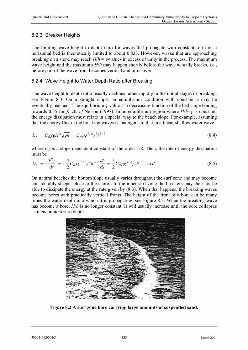
Queensland Government Queensland Climate Change and Community Vulnerability to Tropical CyclonesOcean Hazards Assessment - Stage 1
8.2.3 Breaker Heights
The limiting wave height to depth ratio for waves that propagate with constant form on a horizontal bed is theoretically limited to about 0.833. However, waves that are approaching
breaking on a slope may reach H/h = -values in excess of unity in the process. The maximumwave height and the maximum H/h may happen shortly before the wave actually breaks, i.e., before part of the wave front becomes vertical and turns over.
8.2.4 Wave Height to Water Depth Ratio after Breaking
The wave height to depth ratio usually declines rather rapidly in the initial stages of breaking,
see Figure 8.3. On a straight slope, an equilibrium condition with constant may be
eventually reached. The equilibrium -value is a decreasing function of the bed slope tending
towards 0.55 for 0, cf Nelson (1997). In an equilibrium region where H/h= is constant, the energy dissipation must relate in a special way to the beach slope. For example, assumingthat the energy flux in the breaking waves is analogous to that in a linear shallow water wave
2/522/32 hgCghgHCE f (8.4)
where C is a slope dependent constant of the order 1/8. Then, the rate of energy dissipation must be
tan2
5
2
5 2/322/32/322/3 hgCdx
dhhgC
dx
dED
fE (8.5)
On natural beaches the bottom slope usually varies throughout the surf zone and may becomeconsiderably steeper close to the shore. In the inner surf zone the breakers may then not be able to dissipate the energy at the rate given by (8.3). When that happens, the breaking waves become bores with practically vertical fronts. The height of the front of a bore can be manytimes the water depth into which it is propagating, see Figure 8.2. When the breaking wave has become a bore, H/h is no longer constant. It will usually increase until the bore collapsesas it encounters zero depth.
Figure 8.2 A surf zone bore carrying large amounts of suspended sand.
J0004-PR0001C 133 March 2001

Queensland Government Queensland Climate Change and Community Vulnerability to Tropical CyclonesOcean Hazards Assessment - Stage 1
8.2.5 Surf Beat
Natural waves tend to be "groupy"; i.e. a wave record usually consists of groups of large waves with intervals of smaller wave heights in between. This variation in wave height can drive a corresponding variation in wave setup in general and in the shoreline setup in particular.
These oscillations are called surf beat. The period of surf beats is usually 100 to 300 seconds corresponding to the typical period of the offshore wave groups. The surface elevationamplitude of surf beat is (in contrast to the wind waves) greatest at the shoreline where it mayexceed one metre during storms. See Figure 8.3.
Figure 8.3 An example of surf beat.
The low frequency part of the spectrum, which represents the
surf beat increases towards the shore while the high frequency
part corresponding to wind wave frequencies decays. This
indicates that the surf beat has the nature of standing non-
breaking waves against the shoreline.
8.3 The Shape of the Surf Zone Mean Water Surface
8.3.1 Terminology and Definitions
The instantaneous surface elevations are denoted (x,y,t) where x is shore-normal and y isshore parallel. They are measured from the still water level (SWL) or the still water surface. See Figure 8.4. The still water surface is the plane (on the scale considered), horizontal watersurface that would exist in the absence of wind and waves. It moves up and down relative tothe mean sea level (MSL) with the tide.
The still water depth D is measured from the local bed level to the SWS. The intersectionbetween the SWS and the beach is the still water shoreline. The mean water level (x,y) is
the time average of (x,y,t) over a few minutes, i.e., the corresponding mean water surface
J0004-PR0001C 134 March 2001

Queensland Government Queensland Climate Change and Community Vulnerability to Tropical CyclonesOcean Hazards Assessment - Stage 1
(MWS) does not move up and down with the wind waves but it does move with the tide. The total depth or just depth h is measured to the MWS. As indicated by Figure 8.4, the MWSmay be slightly below the SWS off-shore due to wave set-down. In the surf zone it is above the SWS due to wave setup.
Figure 8.4 Definitions of surf zone levels and depths.
The deviations of the MWS from the plane SWS are due to wind and waves and can be quantified on the basis of Figure 8.5.
Figure 8.5 Time averaged, horizontal forces due to wind, waves and gravity acting on a
surf zone control volume.
J0004-PR0001C 135 March 2001

Queensland Government Queensland Climate Change and Community Vulnerability to Tropical CyclonesOcean Hazards Assessment - Stage 1
The static, shore-normal force balance on the control volume in Figure 8.5 gives
0xbedxwindS xxhg (8.6)
or
)(11
bedwindxx
ghx
S
ghx(8.7)
8.3.2 Wave Setdown
Outside the surf zone, the wave radiation stress will increase towards the shore as indicated bythe sine wave explicit approximation
]18
11[
1
16
3 2 hkhk
gHS o
o
oxx (8.8)
This formula is within 1% of linear wave theory for koh < 0.94.
Inserting this expression for the radiation stress into the slope equation (8.7), neglecting the shear stresses, and integrating with the boundary condition 0 for , we get the
following expression
hko
]6
11[)(
32
1 5.12 hkhkHk oooo (8.9)
for the setdown, i.e. the lowering of the mean water level outside the surf zone. A setdown of this magnitude has often been measured in laboratory experiments with regular waves.
8.3.3 Wave Setup
Inside the surf zone the radiation stress (proportional to H2 for sine waves) will decrease
rapidly towards the shore due to wave breaking and therefore generate a positive MWS slope through Equation (8.7).
A simple model of the wave setup in the surf zone can be obtained by adopting the linear shallow water relation between radiation stress and wave height
2
16
3gHSxx (8.10)
Neglecting the shear stress terms in (8.7) this leads to the slope
x
HH
hx 8
31(8.11)
J0004-PR0001C 136 March 2001

Queensland Government Queensland Climate Change and Community Vulnerability to Tropical CyclonesOcean Hazards Assessment - Stage 1
In order to solve this and get the setup as function of x or h, it is further necessary to assume a
relation between wave height and depth. If we assume a constant ratio H/h , we obtain
x
h
x
2
8
3(8.12)
where we may insert h = D+ and get
)(8
3 2
xx
D
x(8.13)
and hence
tan
8
31
8
3
8
31
8
3
2
2
2
2
x
D
x(8.14)
wherex
Dtan . That is, assuming linear shallow water wave theory and 0.5 for the
breaking waves we would expect a slope of the surf zone MWS of about .09 tan .
Seeking the setup as function of the total depth, we can solve Equation (8.12) with the boundary condition (hb) = min at the breakpoint and get
)(8
3)( 2
min hhh b (8.15)
That is, according to the simple model based on regular waves, Sxx(H) from linear wave
theory and H/h , varies linearly with h. The straight line in Figure 8.6 corresponds to
Equation (8.15), i.e. regular waves, with Sxx(H) from linear shallow water wave theory and for
H/h = 0.5.
The deviation of the data from the straight line is mainly because the real waves are irregular
and start to break at different depths. Hence, the gradual increase in dh
dcompared to the
regular wave model.
The curved line in Figure 8.6 corresponds to the empirical formula
orms
orms
H
h
H
101
4.0(8.16)
which provides a good fit to field data from a wide variety of beach morphologies.
J0004-PR0001C 137 March 2001
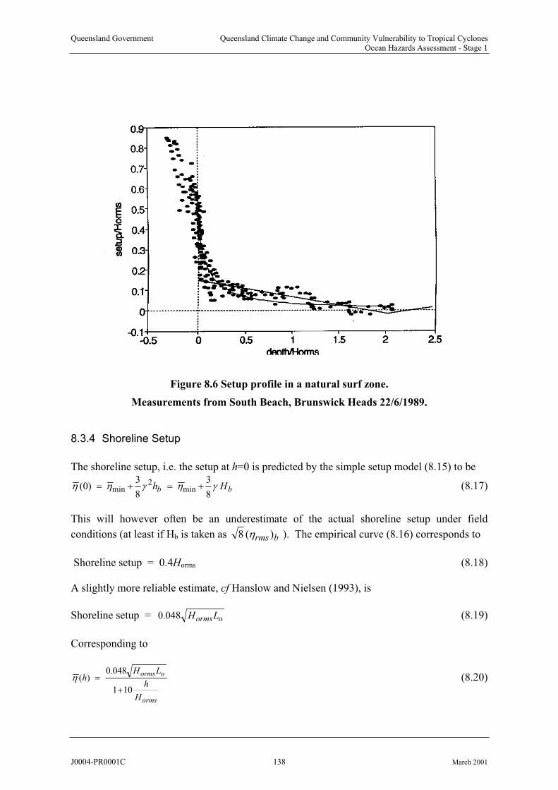
Queensland Government Queensland Climate Change and Community Vulnerability to Tropical CyclonesOcean Hazards Assessment - Stage 1
Figure 8.6 Setup profile in a natural surf zone.
Measurements from South Beach, Brunswick Heads 22/6/1989.
8.3.4 Shoreline Setup
The shoreline setup, i.e. the setup at h=0 is predicted by the simple setup model (8.15) to be
bb Hh8
3
8
3)0( min
2min (8.17)
This will however often be an underestimate of the actual shoreline setup under field
conditions (at least if Hb is taken as brms )(8 ). The empirical curve (8.16) corresponds to
Shoreline setup = 0.4Horms (8.18)
A slightly more reliable estimate, cf Hanslow and Nielsen (1993), is
Shoreline setup = oormsLH048.0 (8.19)
Corresponding to
orms
oorms
H
h
LHh
101
048.0)( (8.20)
J0004-PR0001C 138 March 2001
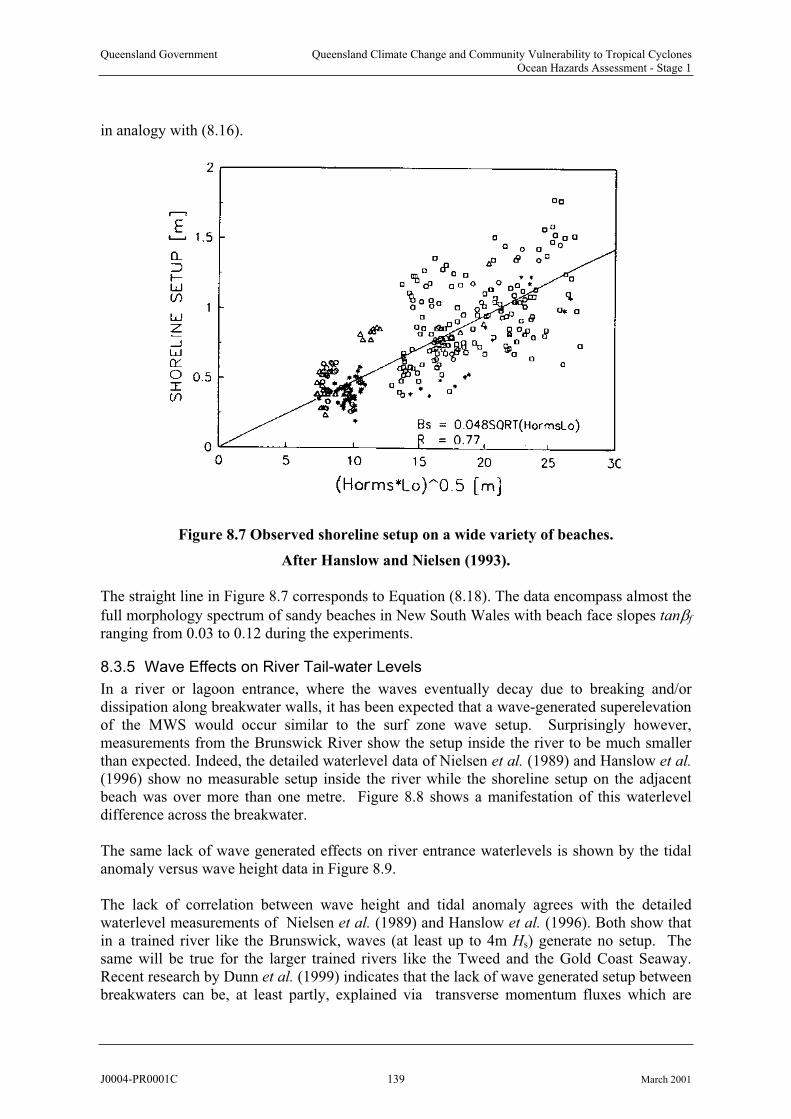
Queensland Government Queensland Climate Change and Community Vulnerability to Tropical CyclonesOcean Hazards Assessment - Stage 1
in analogy with (8.16).
Figure 8.7 Observed shoreline setup on a wide variety of beaches.
After Hanslow and Nielsen (1993).
The straight line in Figure 8.7 corresponds to Equation (8.18). The data encompass almost the
full morphology spectrum of sandy beaches in New South Wales with beach face slopes tan f
ranging from 0.03 to 0.12 during the experiments.
8.3.5 Wave Effects on River Tail-water Levels
In a river or lagoon entrance, where the waves eventually decay due to breaking and/ordissipation along breakwater walls, it has been expected that a wave-generated superelevation of the MWS would occur similar to the surf zone wave setup. Surprisingly however, measurements from the Brunswick River show the setup inside the river to be much smallerthan expected. Indeed, the detailed waterlevel data of Nielsen et al. (1989) and Hanslow et al.
(1996) show no measurable setup inside the river while the shoreline setup on the adjacent beach was over more than one metre. Figure 8.8 shows a manifestation of this waterlevel difference across the breakwater.
The same lack of wave generated effects on river entrance waterlevels is shown by the tidal anomaly versus wave height data in Figure 8.9.
The lack of correlation between wave height and tidal anomaly agrees with the detailedwaterlevel measurements of Nielsen et al. (1989) and Hanslow et al. (1996). Both show that in a trained river like the Brunswick, waves (at least up to 4m Hs) generate no setup. The same will be true for the larger trained rivers like the Tweed and the Gold Coast Seaway. Recent research by Dunn et al. (1999) indicates that the lack of wave generated setup between breakwaters can be, at least partly, explained via transverse momentum fluxes which are
J0004-PR0001C 139 March 2001
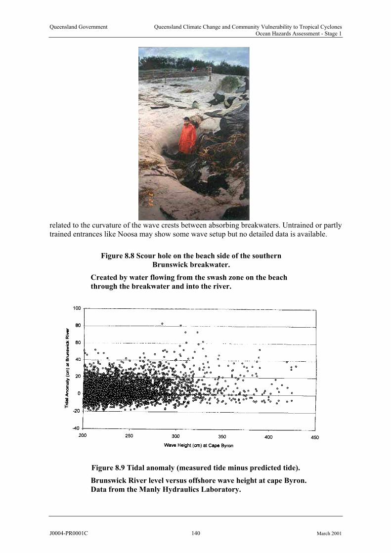
Queensland Government Queensland Climate Change and Community Vulnerability to Tropical CyclonesOcean Hazards Assessment - Stage 1
related to the curvature of the wave crests between absorbing breakwaters. Untrained or partly trained entrances like Noosa may show some wave setup but no detailed data is available.
Figure 8.8 Scour hole on the beach side of the southern
Brunswick breakwater.
Created by water flowing from the swash zone on the beach
through the breakwater and into the river.
Figure 8.9 Tidal anomaly (measured tide minus predicted tide).
Brunswick River level versus offshore wave height at cape Byron.
Data from the Manly Hydraulics Laboratory.
J0004-PR0001C 140 March 2001

Queensland Government Queensland Climate Change and Community Vulnerability to Tropical CyclonesOcean Hazards Assessment - Stage 1
8.4 Swash and Runup Heights
8.4.1 Introduction
The water motion in the area where the beach face is alternately exposed and covered by water on the time scale of individual wind waves is called swash, cf Figure 8.10.
Figure 8.10 Bore collapsing at the beach face where it encounters zero
depth and generating swash.
While the bed slope is usually variable through the surf zone the beach
face is usually straight. Hence the slope tan f of the beach face is well
defined.
The swash is a highly asymmetrical motion where the depth and speed of the uprush isdetermined by the height and speed of the incoming bores while the backwash is driven bygravity. The sand onto which the swash is progressing may be saturated or unsaturated with water depending on the tidal phase and on the strengths of previous uprush events.
If the beach material is very coarse, the swash may also be asymmetrical with respect tovolume. That is, the amount of water running back down the slope is less than what rushed up because a substantial part of the uprush volume has seeped into the slope.
On very flat beaches where breakers of constant form and dissipate energy fast enough (cf
Equation 2.3) to maintain a constant H/h and hence, H 0 for h 0, there will be noswash at wind wave frequencies.
8.4.2 Runup heights for Regular Waves
When the incoming waves are regular having fixed height and period they will all run up to same height on the beach. In this case it makes sense to talk about the runup height R..
J0004-PR0001C 141 March 2001
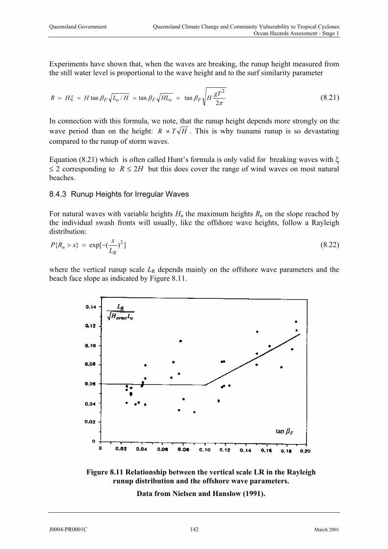
Queensland Government Queensland Climate Change and Community Vulnerability to Tropical CyclonesOcean Hazards Assessment - Stage 1
Experiments have shown that, when the waves are breaking, the runup height measured from the still water level is proportional to the wave height and to the surf similarity parameter
2tantan/tan
2gTHHLHLHHR FoFoF (8.21)
In connection with this formula, we note, that the runup height depends more strongly on the
wave period than on the height: HTR . This is why tsunami runup is so devastating
compared to the runup of storm waves.
Equation (8.21) which is often called Hunt’s formula is only valid for breaking waves with
2 corresponding to R 2H but this does cover the range of wind waves on most natural beaches.
8.4.3 Runup Heights for Irregular Waves
For natural waves with variable heights Hn the maximum heights Rn on the slope reached by the individual swash fronts will usually, like the offshore wave heights, follow a Rayleighdistribution:
])(exp[}{ 2
Rn
L
xxRP (8.22)
where the vertical runup scale LR depends mainly on the offshore wave parameters and the beach face slope as indicated by Figure 8.11.
Figure 8.11 Relationship between the vertical scale LR in the Rayleigh
runup distribution and the offshore wave parameters.
Data from Nielsen and Hanslow (1991).
J0004-PR0001C 142 March 2001

Queensland Government Queensland Climate Change and Community Vulnerability to Tropical CyclonesOcean Hazards Assessment - Stage 1
For steep slopes LR is approximately 0.6 times the runup height of the rms wave calculated from Equation (8.21), i.e.
oormsFR LHL tan6.0 for tan F > 0.1 (8.23)
for flatter slopes LR is independent of F and approximately given by
oormsR LHL 06.0 for tan F < 0.1 (8.24)
According to the definition (8.22), the highest of N individual runup heights is, under theRayleigh distribution, expected to be
NLRE R ln}{ max (8.25)
and the height (above the SWS) exceeded by just 1% of the runups is expected to be
RR LLRE 6.4100ln}{ %1 (8.26)
8.4.4 Extreme Runup Levels
The expected maximum runup level from N waves with a given LR is according to (8.25)
NLR ln . This level has roughly a 50% probability of getting inundated (reached at least once)
by these waves.
It is of interest to calculate the level Z which has a certain probability P of getting inundated during an event that contains N waves with a certain LR. This can be done as follows
The probability of a given wave stopping below Z is ])(exp[ 2
RL
Z1 . Consequently, the
probability of all of the N waves stopping below Z is N
RL
Z])(exp[ 21 . Hence, the level ZP
that has probability P of being inundated is determined from N
RL
ZP ])(exp[11 2 (8.27)
or
])1(1ln[ /1 NRP PLZ (8.28)
Example:
Extreme wave heights of 4.95m Horms (7m Hs) typically occur for one or two hours per yearalong the east coast of Australia. The period varies, but T=11s is not atypical.. For beaches
with moderate slopes (tan f < 0.1) this corresponds to LR = 1.83m according to (8.24).
For a duration of one hour, the total number of waves is N = 3600/11 = 327.
J0004-PR0001C 143 March 2001
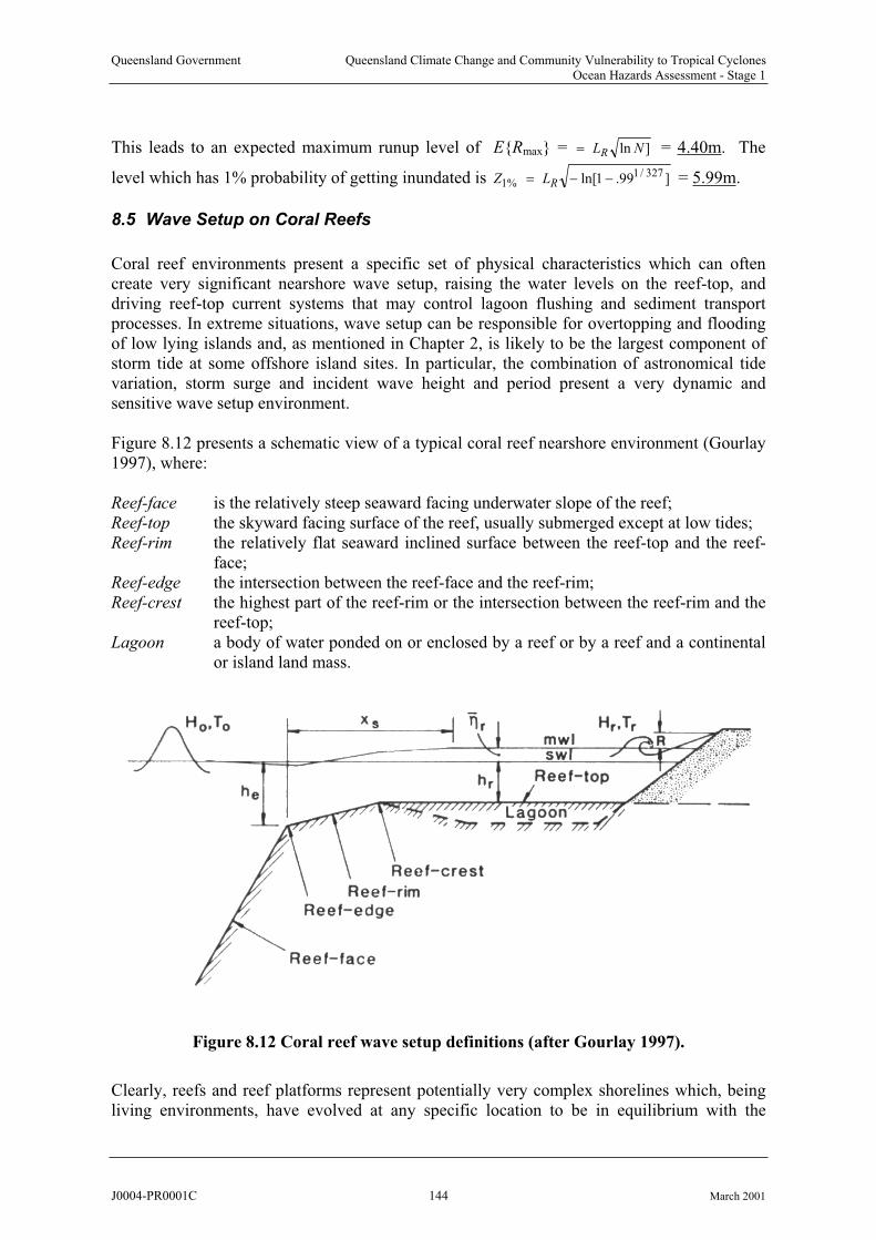
Queensland Government Queensland Climate Change and Community Vulnerability to Tropical CyclonesOcean Hazards Assessment - Stage 1
This leads to an expected maximum runup level of E{Rmax} = ]ln NLR = 4.40m. The
level which has 1% probability of getting inundated is ]99.1ln[ 327/1%1 RLZ = 5.99m.
8.5 Wave Setup on Coral Reefs
Coral reef environments present a specific set of physical characteristics which can often create very significant nearshore wave setup, raising the water levels on the reef-top, anddriving reef-top current systems that may control lagoon flushing and sediment transport processes. In extreme situations, wave setup can be responsible for overtopping and flooding of low lying islands and, as mentioned in Chapter 2, is likely to be the largest component of storm tide at some offshore island sites. In particular, the combination of astronomical tidevariation, storm surge and incident wave height and period present a very dynamic and sensitive wave setup environment.
Figure 8.12 presents a schematic view of a typical coral reef nearshore environment (Gourlay 1997), where:
Reef-face is the relatively steep seaward facing underwater slope of the reef; Reef-top the skyward facing surface of the reef, usually submerged except at low tides; Reef-rim the relatively flat seaward inclined surface between the reef-top and the reef-
face;Reef-edge the intersection between the reef-face and the reef-rim;Reef-crest the highest part of the reef-rim or the intersection between the reef-rim and the
reef-top;Lagoon a body of water ponded on or enclosed by a reef or by a reef and a continental
or island land mass.
Figure 8.12 Coral reef wave setup definitions (after Gourlay 1997).
Clearly, reefs and reef platforms represent potentially very complex shorelines which, beingliving environments, have evolved at any specific location to be in equilibrium with the
J0004-PR0001C 144 March 2001

Queensland Government Queensland Climate Change and Community Vulnerability to Tropical CyclonesOcean Hazards Assessment - Stage 1
incident wave and tide conditions. Even relatively small areas of reef platforms may display a myriad of channels, ridges and holes. Any estimate of wave setup must therefore beconsidered in a very generalised manner and applied with caution to specific locations. In particular, accurate information on reef-top water levels and slopes will be seen to be critical to any accurate assessment of reef setup.
Using an analysis combining wave energy flux and radiation stress concepts, Gourlay (1994b)
derived the following equation for the wave setup r
rh
on a reef-top as a function of the offreef
wave conditions and T and the stillwater depth on the reef top: oH
g
h
TKK
h
THgK rr
Rr
rr
opr
)(141
)(64
3 22
2/3
22/1
(8.29)
where is a reef profile factor (varies according to reef profile up to approximately 0.8) pK
is the reflection coefficient (0 to 1) RK
is the transmission coefficient (0 to 1)rK
and the term in [...] is subsequently referred to as the transmission parameter .TP
Laboratory experiments (Gourlay 1996a) indicate that for steep reef-faces , whereas
for flatter slopes (Gourlay 1994) . Hence wave reflection at most decreases the wave
setup by about 10% and can be reasonably neglected.
3.0RK
1.0RK
The influence of wave transmission on wave setup however is a function of the relativesubmergence S, viz.
o
rr
H
hS
)((8.30)
and is also relatively small when S < 1. However it becomes increasingly significant as the
submergence increases until, when S 2.5, waves pass over the reef without breaking and hence without generating any setup (Gourlay 1996a).
To facilitate analysis, the transmission coefficient can be expressed in terms
of the reef-top wave height to depth ratio
)/( orr HHK
))(/ rrr hH(r . The resulting form of the
transmission parameter , neglecting , is then:TP RK
o
rrrrrT
H
h
g
h
TP
)()(141
2
2 (8.31)
or
DSP rT /41 22 (8.32)
J0004-PR0001C 145 March 2001
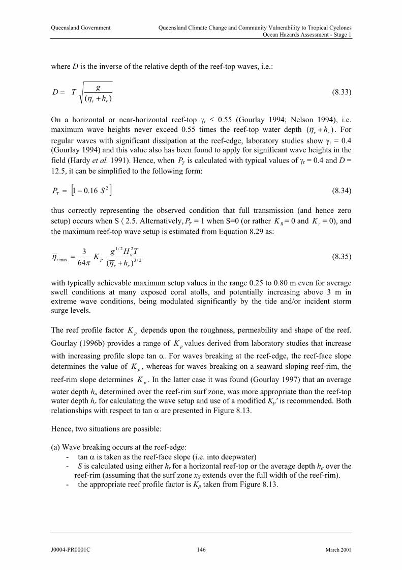
Queensland Government Queensland Climate Change and Community Vulnerability to Tropical CyclonesOcean Hazards Assessment - Stage 1
where D is the inverse of the relative depth of the reef-top waves, i.e.:
)( rr h
gTD (8.33)
On a horizontal or near-horizontal reef-top r 0.55 (Gourlay 1994; Nelson 1994), i.e.
maximum wave heights never exceed 0.55 times the reef-top water depth )rr h( . For
regular waves with significant dissipation at the reef-edge, laboratory studies show r = 0.4 (Gourlay 1994) and this value also has been found to apply for significant wave heights in the
field (Hardy et al. 1991). Hence, when is calculated with typical values ofTP r = 0.4 and D =
12.5, it can be simplified to the following form:
216.01 SPT (8.34)
thus correctly representing the observed condition that full transmission (and hence zero
setup) occurs when S 2.5. Alternatively, = 1 when S=0 (or rather = 0 and = 0), and
the maximum reef-top wave setup is estimated from Equation 8.29 as: TP RK rK
2/3
22/1
max)(64
3
rr
opr
h
THgK (8.35)
with typically achievable maximum setup values in the range 0.25 to 0.80 m even for average swell conditions at many exposed coral atolls, and potentially increasing above 3 m in extreme wave conditions, being modulated significantly by the tide and/or incident storm surge levels.
The reef profile factor depends upon the roughness, permeability and shape of the reef.
Gourlay (1996b) provides a range of values derived from laboratory studies that increase
with increasing profile slope tan . For waves breaking at the reef-edge, the reef-face slope
determines the value of , whereas for waves breaking on a seaward sloping reef-rim, the
reef-rim slope determines . In the latter case it was found (Gourlay 1997) that an average
water depth h
pK
pK
pK
pK
a determined over the reef-rim surf zone, was more appropriate than the reef-topwater depth hr for calculating the wave setup and use of a modified Kp' is recommended. Both
relationships with respect to tan are presented in Figure 8.13.
Hence, two situations are possible:
(a) Wave breaking occurs at the reef-edge:
- tan is taken as the reef-face slope (i.e. into deepwater) - S is calculated using either hr for a horizontal reef-top or the average depth ha over the
reef-rim (assuming that the surf zone xS extends over the full width of the reef-rim).- the appropriate reef profile factor is Kp taken from Figure 8.13.
J0004-PR0001C 146 March 2001

Queensland Government Queensland Climate Change and Community Vulnerability to Tropical CyclonesOcean Hazards Assessment - Stage 1
Figure 8.13 Kp and Kp' as a function of tan (after Gourlay 1997).
(b) Wave breaking occurs at the reef-rim:- the breakpoint should be calculated (i.e. the breaker depth related to the reef-rim
slope)- S is calculated using the average depth hba on the reef-rim between the breakpoint and
the reef-crest (or for tan > 0.1, between the inner and outer surf zones) - the appropriate reef profile factor is Kp' taken from Figure 8.13.
In the latter situation, the breakpoint depth (d = db) can be estimated as proposed by Gourlay (1992), ignoring possible wave-setdown, viz:
17.0
2tan259.0o
o
o
b
L
H
H
d(8.36)
Furthermore, calculation of ha or hab implies knowledge of the surf zone width xS which can be estimated by the following equation from Gourlay (1994):
e
e
oS hgT
h
Hx 1.12 (8.37)
where he is the reef-edge depth.
Finally, irregular waves may be considered in an analogous manner, substituting the offreef wave parameters as follows, e.g.
20
osrmso
HHH (8.38)
J0004-PR0001C 147 March 2001
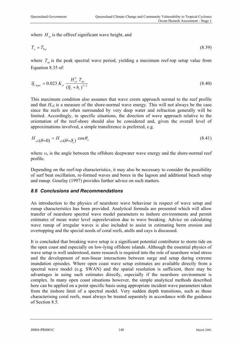
Queensland Government Queensland Climate Change and Community Vulnerability to Tropical CyclonesOcean Hazards Assessment - Stage 1
where is the offreef significant wave height, and osH
po TT 0 (8.39)
where is the peak spectral wave period, yielding a maximum reef-top setup value from
Equation 8.35 of:
opT
2/3
2
max)(
023.0rr
opos
prh
THK (8.40)
This maximum condition also assumes that wave crests approach normal to the reef profileand that HoS is a measure of the shore-normal wave energy. This will not always be the casesince the reefs are often surrounded by very deep water and refraction generally will belimited. Accordingly, in specific situations, the direction of wave approach relative to theorientation of the reef-shore should also be considered and, given the overall level of approximations involved, a simple transference is preferred, e.g.
oo
oSoSHH cos
)()0((8.41)
where o is the angle between the offshore deepwater wave energy and the shore-normal reef profile.
Depending on the reef-top characteristics, it may also be necessary to consider the possibilityof surf beat oscillation, re-formed waves and bores in the lagoon and additional beach setup and runup. Gourlay (1997) provides further advice on such matters.
8.6 Conclusions and Recommendations
An introduction to the physics of nearshore wave behaviour in respect of wave setup and runup characteristics has been provided. Analytical formula are presented which will allow transfer of nearshore spectral wave model parameters to inshore environments and permitestimates of mean water level superelevation due to wave breaking. Advice on calculatingwave runup of irregular waves is also included to assist in estimating berm erosion and overtopping and the special needs of coral reefs, atolls and cays is discussed.
It is concluded that breaking wave setup is a significant potential contributor to storm tide on the open coast and especially on low-lying offshore islands. Although the essential physics of wave setup is well understood, more research is required into the role of nearshore wind stress and the development of non-linear interactions between surge and setup during extremeinundation episodes. Where open coast wave setup estimates are available directly from aspectral wave model (e.g. SWAN) and the spatial resolution is sufficient, there may be advantages in using such estimates directly, especially if the nearshore environment is complex. In many open coast situations however, the simple analytical methods described here can be applied on a point specific basis using appropriate incident wave parameters taken from the inshore limit of a spectral model. Very sudden depth transitions, such as those characterising coral reefs, must always be treated separately in accordance with the guidance of Section 8.5.
J0004-PR0001C 148 March 2001

Queensland Government Queensland Climate Change and Community Vulnerability to Tropical CyclonesOcean Hazards Assessment - Stage 1
It is recommended that (a) analytical methods be applied to the estimation of wave setup
using nearshore spectral wave model output parameters and that this be applied at a fine
scale resolution (e.g. C grid minimum, refer Chapter 11) and (b) that further research be
initiated into the nearshore physics of extreme inundation episodes so as to provide better
guidance for the likely significant community impacts.
8.7 References
Booij, N., Holthuijsen, L.H. and Ris, R.C. (1996) The SWAN wave model for shallow water. Proc 25th Int. Conf. Coastal Eng., ASCE, Orlando, 668-676.
Dunn S.L., Nielsen P. and Madsen P.A.(1999) Wave setup in jettied river entrances. Coasts and Ports ’99: Proc 14th Australasian Coastal and Ocean Engineering Conference, Perth, WA,April 14-16, IEAust, 193-198.
Gourlay M.R. (1992) Wave set-up, wave run-up and beach water table: Interaction between surf zone hydraulics and groundwater hydraulics. Coastal Engineering, 17, 93-144.
Gourlay M.R. (1994) Wave transformation on a coral reef. Coastal Engineering, 23,17-42.
Gourlay M.R. (1996a) Wave setup on coral reefs. 1. Set-up and wave-generated flow on an idealised two dimensional horizontal reef. Coastal Engineering, 27,161-193.
Gourlay M.R. (1996b) Wave setup on coral reefs. 1. Set-up on reefs with various profiles. Coastal Engineering, 28, 17-55.
Gourlay M.R. (1997) Wave setup on coral reefs: some practical applications. Proc. 13th Australasian Conf Coastal and Ocean Engin., IEAust, Christchurch, Sep, 959-964.
Hanslow D.J. and Nielsen P. (1993) Shoreline setup on natural beaches. J Coastal Res,
Special Issue 15, 1-10.
Hanslow D.J., Nielsen P. and Hibbert K. (1996) Wave setup at river entrances. Proc 25th Int Conf Coastal Eng, Orlando, September 1996, ASCE, 2244-2257.
Hardy T.A., Young I.R., Nelson R.C. and Gourlay M.R. (1991) Wave attenuation on an offshore coral reef. Proc. 22nd Intl Conf Coastal Engin., Delft, 1990, ASCE, New York, Vol 1, 330-344.
Nelson R.C. (1994) Depth limited design wave heights in very flat regions. Coastal
Engineering, 23, 43-59.
Nielsen, P (1989) Measurements of wave setup and the watertable in beaches. Proc 9th Australasian Conf Coastal and Ocean Eng, Adelaide, IEAust, 275-279.
Nielsen P. and Hanslow D.J. (1991) Wave runup distributions on natural beaches. J Coastal
Res, Vol 7, No 4, pp 1139-1152.
J0004-PR0001C 149 March 2001
Queensland Government Queensland Climate Change and Community Vulnerability to Tropical CyclonesOcean Hazards Assessment - Stage 1
9. Storm Tide Statistics
9.1 Introduction
The expected long-term spatial and temporal variability of storm tide threats along a coastline can only be described statistically. Storm tide statistics then express the potential magnitude and duration of specific weather events in a mathematical context which accounts for the likelihood of experiencing storms which locally exceed certain intensity thresholds, combinedwith the presence of the astronomical tide. This requires measures of the natural variability of climate as well as the potential additional effects of Greenhouse-induced long-term climatechange.
Knowledge of storm tide statistics is essential for sustainable economic development in the coastal zone and their potential application covers a diverse range of planning and investigation needs, viz
Community vulnerability and emergency planning:
Inundation mapping
Risk assessment of community housing and infrastructure
Disaster cost estimation and design of insurance products
Evacuation planning (onshore and offshore)
Tourism and environmental values:
Protection of natural coastal systems (dunes, coastal lakes and wetlands etc)
Extreme weather impacts on the Great Barrier Reef
World heritage custodianship best practice
Establishment of development control (buffer) zones
Coastal management, port infrastructure design and maintenance:
Long term coastal erosion and accretion studies
Beach nourishment programs
Design criteria for fixed and floating structures, e.g. bridges, jetties, wharfs, breakwaters,revetments, pontoons, moorings
Navigation needs, e.g. inlet and channel stability
Harbour operations, e.g. port closure planning, dredging strategies
Artificial waterways, e.g. canal estates
Aquaculture
This section discusses a range of methodologies which are available for computing storm tide statistics, including requirements to take into account climate change, sea level rise, anddecadal variability in cyclones. Recommendations are made as to the most appropriatetechnical options in the Queensland context and in regard to the overall aims of the present project.
9.2 The Historical Context
The threat of inundation and potential for loss of life from storm tide disasters was already evident from our earliest historical experience, much of which was chronicled by
J0004-PR0001C 150 March 2001

Queensland Government Queensland Climate Change and Community Vulnerability to Tropical CyclonesOcean Hazards Assessment - Stage 1
Whittingham (1958, 1959, 1968) and Holthouse (1971) in regard to the famous 1899 Bathurst Bay and other significant events. Awareness of and interest in the ability to make predictionsabout the variation in storm surge characteristics around the Australian coast began in the late 1960s. This was supported by the advances in the USA where similar storm tide threats were being experienced along the rapidly developing Gulf of Mexico and Atlantic coastlines. Thisawareness had been fuelled by the significant outcomes in regard to meteorology and climatology of hurricanes from the US National Hurricane Research Project (Graham and Nunn 1959). The Shore Protection Manual (CERC 1966) provided basic design advice which was soon updated and extended by the work of many researchers such as Bretschneider (1967), Jelesnianski (1965, 1972). Nickerson (1971) formalised a manual estimation methodfor storm surges based on results from the Jelesnianski numerical modelling.
In the Australian context, tropical cyclone Althea in 1971 at Townsville provided a degree ofurgency in understanding these phenomena and Stark (1972) provided a valuable primer formany subsequent studies. Initial work by the Bureau of Meteorology (Trajer 1973) adopted the Nickerson nomogram technique for the Southern Hemisphere and it has remained a useful operational tool to the present time (Callaghan 2000). This research was continued by Dexter (1975) who was among the first to consider statistical methods for estimating the potential variability of surge magnitudes and Nelson (1975) provided one of the earliest compendiumsof historical surge data. Meanwhile Hopley and Harvey (1976) undertook extensive tidal data analyses and provided an Australia-wide perspective that provided some potential insight intothe regional variability, together with Silvester and Mitchell (1977) who utilised a simplified modelling approach. None of the above studies, though, was sufficiently sophisticated to enable estimation of true storm tide statistics, i.e. the consideration of the very significant influence of the astronomical tide on the total mean water level.
From the mid-1970s onwards studies increasingly addressed the astronomical tide problemand began to provide predictions for a range of locations in Queensland. The techniques increased in complexity as access to computing facilities expanded and simulation-basedapproaches became more tractable. Table 9.1 provides a brief overview of progress over the past 25 years, taken predominantly from the recent review by Harper (1999a), while the actual methodologies are discussed in detail in subsequent sections. The main client organisation during this time was the Beach Protection Authority of Queensland (now a part of the Environmental Protection Agency) with a specific interest in the long-term behaviour of the coastal system. Other clients have included specific Local Government Authorities or privateinfrastructure developers requiring design information.
Some of the earlier studies (b) and (c) utilised analytical treatments of the "conditionalprobability" of combinations of water levels due to storm surge and the astronomical tide. Inthis case, the deterministic storm surge estimates were derived from the simplified nomogramtechnique of Nickerson (1971). The simulation techniques based on site-specific numericalhydrodynamic modelling, such as those indicated above as "Monte Carlo" approaches, were developing at that time (e.g. Russell 1971) and offered greater accuracy with fewerassumptions than the approximate analytical approaches. The reliance on simplifiednomogram techniques became supplanted by the development of Australia's first generalisednumerical hydrodynamic model of storm surges developed in the late 1970s by James Cook University (Sobey et al., 1977; Harper et al. 1977). This model provided the means to construct site-specific "nomograms" for the Queensland coast based on a range of modelled "design" storms.
J0004-PR0001C 151 March 2001
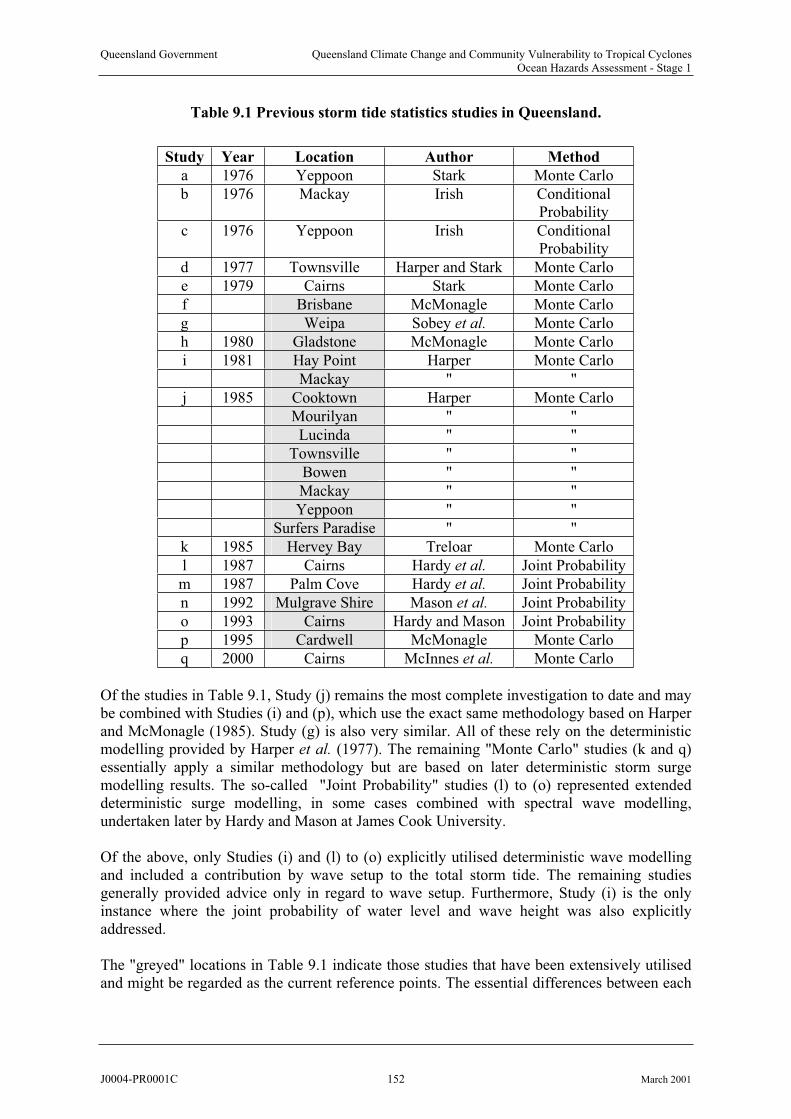
Queensland Government Queensland Climate Change and Community Vulnerability to Tropical CyclonesOcean Hazards Assessment - Stage 1
Table 9.1 Previous storm tide statistics studies in Queensland.
Study Year Location Author Method
a 1976 Yeppoon Stark Monte Carlo
b 1976 Mackay Irish ConditionalProbability
c 1976 Yeppoon Irish ConditionalProbability
d 1977 Townsville Harper and Stark Monte Carlo
e 1979 Cairns Stark Monte Carlo
f Brisbane McMonagle Monte Carlo
g Weipa Sobey et al. Monte Carlo
h 1980 Gladstone McMonagle Monte Carlo
i 1981 Hay Point Harper Monte Carlo
Mackay " "
j 1985 Cooktown Harper Monte Carlo
Mourilyan " "
Lucinda " "
Townsville " "
Bowen " "
Mackay " "
Yeppoon " "
Surfers Paradise " "
k 1985 Hervey Bay Treloar Monte Carlo
l 1987 Cairns Hardy et al. Joint Probability
m 1987 Palm Cove Hardy et al. Joint Probability
n 1992 Mulgrave Shire Mason et al. Joint Probability
o 1993 Cairns Hardy and Mason Joint Probability
p 1995 Cardwell McMonagle Monte Carlo
q 2000 Cairns McInnes et al. Monte Carlo
Of the studies in Table 9.1, Study (j) remains the most complete investigation to date and maybe combined with Studies (i) and (p), which use the exact same methodology based on Harper and McMonagle (1985). Study (g) is also very similar. All of these rely on the deterministicmodelling provided by Harper et al. (1977). The remaining "Monte Carlo" studies (k and q) essentially apply a similar methodology but are based on later deterministic storm surge modelling results. The so-called "Joint Probability" studies (l) to (o) represented extendeddeterministic surge modelling, in some cases combined with spectral wave modelling,undertaken later by Hardy and Mason at James Cook University.
Of the above, only Studies (i) and (l) to (o) explicitly utilised deterministic wave modellingand included a contribution by wave setup to the total storm tide. The remaining studies generally provided advice only in regard to wave setup. Furthermore, Study (i) is the only instance where the joint probability of water level and wave height was also explicitlyaddressed.
The "greyed" locations in Table 9.1 indicate those studies that have been extensively utilised and might be regarded as the current reference points. The essential differences between each
J0004-PR0001C 152 March 2001
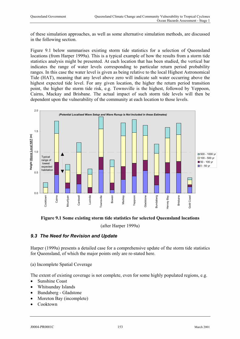
Queensland Government Queensland Climate Change and Community Vulnerability to Tropical CyclonesOcean Hazards Assessment - Stage 1
of these simulation approaches, as well as some alternative simulation methods, are discussed in the following section.
Figure 9.1 below summarises existing storm tide statistics for a selection of Queenslandlocations (from Harper 1999a). This is a typical example of how the results from a storm tide statistics analysis might be presented. At each location that has been studied, the vertical bar indicates the range of water levels corresponding to particular return period probability ranges. In this case the water level is given as being relative to the local Highest AstronomicalTide (HAT), meaning that any level above zero will indicate salt water occurring above the highest expected tide level. For any given location, the higher the return period transition point, the higher the storm tide risk, e.g. Townsville is the highest, followed by Yeppoon, Cairns, Mackay and Brisbane. The actual impact of such storm tide levels will then be dependent upon the vulnerability of the community at each location to those levels.
0.0
0.5
1.0
1.5
2.0
Cookto
wn
Cairns
Mourily
an
Card
well
Lucin
da
To
wn
svill
e
Bow
en
Mackay
Yeppoon
Gla
dsto
ne
Bundaberg
Herv
ey B
ay
Brisbane
Gold
Coast
Heig
ht
Ab
ove L
ocal H
AT
(m
)
500 - 1000 yr
100 - 500 yr
50 - 100 yr
0 - 50 yr
Typical
range of
lowest
expected
habitation
(Potential Localised Wave Setup and Wave Runup is Not Included in these Estimates)
Figure 9.1 Some existing storm tide statistics for selected Queensland locations
(after Harper 1999a)
9.3 The Need for Revision and Update
Harper (1999a) presents a detailed case for a comprehensive update of the storm tide statisticsfor Queensland, of which the major points only are re-stated here.
(a) Incomplete Spatial Coverage
The extent of existing coverage is not complete, even for some highly populated regions, e.g.
Sunshine Coast
Whitsunday Islands
Bundaberg - Gladstone
Moreton Bay (incomplete)
Cooktown
J0004-PR0001C 153 March 2001
Queensland Government Queensland Climate Change and Community Vulnerability to Tropical CyclonesOcean Hazards Assessment - Stage 1
Gulf of Carpentaria
Torres Strait
(b) Differences in Basic Methodology
The techniques and models for undertaking storm surge analyses have developed since the mid 1970s with improved models of the tropical cyclone wind field now available, which will create slightly different surge responses for the same set of parameters. Numericalhydrodynamic models of surge have also progressed during this period with improved boundary conditions and allowance for overland flow where justified. Three dimensional modelling may now also be applied where necessary. Access to increased computational power also allows finer scale representation of coastal forms, wider parameter ranges, greater numbers of scenarios, modelling over longer periods and potential for inclusion of simultaneous tide, wave and current effects.
(c) Increased and Better Cyclone Data
The earliest statistical studies were limited by the climatological record of the time with themajority dependant on Lourensz (1981). However, following work by Holland (1981) it is now generally acknowledged that cyclone data in the Australian region can only be regarded as reasonably reliable since 1959/60 when the first satellite surveillance commenced. The ability to revise older cyclone data and more easily examine measured wind and pressure data has enabled the historical track details to be enhanced in some cases.
(d) Climate Change Scenarios
Only two of the existing studies have considered allowance for Greenhouse-induced climatescenarios and none consider inter-decadal variability. All of the other existing studies assumea static mean sea level based on present climate conditions. The impact of the changing statistical data set and scenarios of climate change or sea level rise could only be assessed by reworking present water level predictions.
(e) Increased Measured Data on Storm Tides
Over time an increasing number of significant storm tide events have been measured whichprovide opportunities for better model calibration and to provide insight into the potentialinteractions between surge, tides and waves.
(f) Wave Setup, Runup and Inundation
The existing studies covered large sections of coast and, commensurate with the scale of thestorm surge itself, did not address fine scale details at any of the coastal sites. These include the local effect of wave setup, runup and overland flooding - all of which can have significant counter disaster ramifications. Few of the existing studies included explicit ocean wave modelling in the estimation of wave-induced setup and only one considered overland flooding.
(g) Non-Cyclonic Storm Tide Influences
J0004-PR0001C 154 March 2001
Queensland Government Queensland Climate Change and Community Vulnerability to Tropical CyclonesOcean Hazards Assessment - Stage 1
Significant non-cyclonic weather events, such as monsoonal surges or deep extra-tropical systems, are capable of producing smaller but often more prolonged increases in coastal water levels. These may be responsible for more frequent episodes where the elevation of water levels reaches or just exceeds HAT. Longer duration is a critical factor for beach erosion andbecause of their potential linkage to episodes of heavy rain, such events are more likely to beassociated with flooding. The Surfers Paradise storm tide predictions (Harper 1985) are the only case that presently includes some allowance for these effects.
9.4 The Prediction Problem
Traditional methods for estimating the probability of occurrence of extreme weather events (e.g. floods, winds, waves) are normally based on the statistical analysis of data. In manysituations involving environmental processes, however, the data available for such analysis istypically incomplete, unrepresentative, often scant and, at worst, non-existent. For example,the estimation of extreme tropical cyclone wind speeds based only on recorded data is often inadequate for use in specialist engineering design (Harper 1999b). Firstly, the period of reliable data record at many sites is still relatively short (rarely exceeding 50 years) and the spatial separation of individual data sites is large. Secondly, the range of potential cyclone intensities can be high, their occurrence is typically very low and their area of influence relatively small. Even where reliable recorded data is available, extrapolation to long returnperiods (low probability levels) is problematical and retention of an associated parameter such as direction or persistence to any level of accuracy is difficult. Also, the statistical wind recorditself does not contain explicit guidance on questions such as climate change, and is notdirectly suitable for other design considerations such as the determination of extreme wave heights and storm surge. Knowledge of the meteorological system and its applicable time and space scales then becomes of paramount importance rather than the isolated analysis of specific, and sometimes inadequate, site-specific records of its incidence. This is not to saythat the data record should be ignored, but rather used as a valuable independent measure of the success of other indirect methods.
In the storm tide context, the astronomical tide component is quite precisely known at manylocations because of its periodic gravity forcing on the planetary scale. Tidal prediction to an accuracy similar to the normal ability to measure it (sub-millimetre) requires harmonicanalysis of a period of about 19 years of measured data. Such analyses have already been completed, except for some notable exceptions in the more remote regions of Australia, and they underpin the routine prediction of tides on a daily basis. By contrast, meteorologicallyforced deviations from the planetary motions occur daily and generate water-level anomalieson both regional and local time and space scales, but these variations are specifically removedby the tidal analysis procedures. Examples include the daily synoptic variation in atmosphericpressure due to solar heating, coastally trapped edge-waves and the like. The storm surge issimply the most dramatic manifestation of these meteorologically forced ocean water levelevents. However, its rarity means that the measurement record at any single coastal site yields insufficient instances to enable the use of traditional data extrapolation techniques. This situation is unlikely to change until many hundreds of years of data becomes available, by which time data stationarity assumptions will likely be violated due to the longer term impactof climate change, whether anthropogenic or natural. In spite of this, some researchers regardthe historical record is adequate for such purposes in some special cases which can draw on stable antiquity data (Van Gelder 1996). In theory, paleo-climate analyses can also assist in
J0004-PR0001C 155 March 2001

Queensland Government Queensland Climate Change and Community Vulnerability to Tropical CyclonesOcean Hazards Assessment - Stage 1
such assessments but the base data is often much filtered by the geological record and is bestutilised as a general trend comparison rather than a site-specific quantitative prediction.
9.5 Estimation of Risks Without Long-Term Measured Data
Alternatives to the analysis of measured data for storm surge estimation are discussed here inthe historical context of their development, allied with the parallel development needs forestimating design wind and wave conditions.
9.5.1 The "Design Storm" Approach
These basic data inadequacies have been recognised for a long time and led to philosophical considerations in the 1960s that considered so-called indirect methods of estimation of the parameters of interest. The first of these became known as the “design storm” approach. The probable maximum hurricane (US Weather Bureau 1968) is an upper-limit example of such a philosophy, which arose as a useful technique for establishing some type of regional benchmark. Typically, a "design storm" intensity would be based on an initial statistical assessment of the probability of such an occurrence within the area of interest, using nominalscales of storm influence. For example, Coleman (1972) provided the relevant climatology in the Australian context, from which an extreme value analysis of intensity could beconstructed for a coastal region. Such a storm would then be a priori aligned along the mostunfavourable track relative to the site of interest to provide a “worst case” scenario for a given storm intensity. This approach provides a potentially very conservative estimate of the associated return period of the winds, waves or storm surge being experienced at a specificpoint because the joint probability of intensity and proximity to site is not considered.
9.5.2 The "Hindcast" Approach
As computer modelling became more readily available through the 1970s, the “design storm”was replaced by the “hindcast” technique. This would involve selecting a number of extremeevents from the record that would have been likely to have affected the site in question, but were not captured by a recording system at the time. Modelling of these events usinghistorical track information then yielded a synthetic time series data set which, with sufficientsamples, was amenable to traditional statistical extreme value extrapolation techniques. Suchan approach was advocated by Dexter (1975) in response to the limitations of the design storm approach. This technique is reasonable for peak wind, wave and storm surge prediction when an adequate historical track record is available but fails in cases where the record issparse, and the resulting predictions can be very site and data sensitive. Storm tide however remains additionally complicated by the simultaneous occurrence of the astronomical tide,which cannot be usefully incorporated directly into the hindcast technique and remains as a necessary analysis add-on. Dexter et al. (1977) provides a review of some Australian progress at this time, noting that the hybrid method of Irish (1977) offered a rational basis for estimating the influence of tidal variability. This involved analytically combining thefrequency distribution for storm surge, estimated from a hindcast perspective, with thefrequency distribution of the predicted tide at the location of interest. Unfortunately a numberof time and space scale assumptions are needed in such an analysis which detract from its utility compared with the methods to be adopted later. The hindcast approach continued to be developed, most notably for the estimation of design wave conditions in deep water (e.g. Ward et al. 1979; Wyland and Thornton 1991) where water level variation can be ignored.
J0004-PR0001C 156 March 2001
Queensland Government Queensland Climate Change and Community Vulnerability to Tropical CyclonesOcean Hazards Assessment - Stage 1
9.5.3 Simulation Techniques
At about the same time, simulation techniques came to be developed in an attempt to overcome the deficiencies of the other indirect methods. Their attraction lay in an ability to represent the processes at work rather than just the outcomes and, specifically, the capacity tocorrectly consider joint probability. This shifted focus away from the strict mathematical artof statistical extrapolation of site-specific scalar data towards a closer look at the possible underlying environmental mechanisms. Simulation techniques offer not only the best way ofestimating extreme wind speed climates but the only reasonable way of doing so out to the long return periods (in excess of 2000 years) increasingly being demanded by today’s risk managers. Three variants are discussed at this point - Monte Carlo, Joint Probability andEmpirical Simulation.
The basic approaches in each case are as follows:
(a) Monte Carlo Methods (MCM) typically construct a complete artificial time history ofstorm tide events (surge + tide + setup) which are based on a discretely (i.e. individually) sampled storm climatology. Normally, each major climate parameter is assumed independent of any others (e.g. p0, R, Vfm etc). In theory, the statistical interpretation can be reserved until the end of the generation phase where probability of exceedance is the typical outcome. Inpractice, the statistical analysis is performed in parallel with the generation and provides the criteria for acceptance of convergence of the outcome at a return period of interest. Themethod relies on the use of simplified (computationally efficient) parametric models for storm tide because of the very large number of realisations required. It does however allow considerable freedom in parameter selection and scenario development.
(b) Joint Probability Methods (JPM) are a logical improvement over the design storm approach whereby the technique seeks to apply detailed storm tide modelling to a specific sitebut only for a discrete range of storm conditions. To do this efficiently it needs to adopt a restricted storm climatology. Unlike the MCM, a complete time history of storm tide events does not need to be generated but rather a series of discrete episodes are assembled (e.g. p0=p1; R=r1; Vfm=v1 etc) whose individual probability of occurrence is assignable. The overall probability of water level exceedance can then be derived by combining the probabilities of each of the episodes when the individual storm tide responses are known. In essence the parameterisation is applied to the climatology rather than the storm tide calculation. The intention with JPM is to avoid redundancy in the storm generation phase because only the onerealisation of a set of storm parameters needs to be modelled to generate the storm tide. Theprobability quantum of each storm tide episode can also be adjusted under scenario testing without necessarily reworking the detailed storm tide analyses. Random tide phasing muststill be introduced separately in the analysis to obtain the total water level statistics.
(c) Empirical Simulation Techniques (EST) seek to bypass the traditional parameterisation of the climatology through a holistic assessment of the historical storm lifecycle data set. Spatial and temporal analysis of the climatology is undertaken to develop what is essentially an extended hindcast data set of storms. This is intended to retain "natural" characteristics of the data set such as curved paths and to preserve the dominant joint probabilities of variousparameters. Essentially the effort with EST is put into the climatology and thereafter is similarto JPM in that detailed storm tide modelling is applied to each event. A quoted advantage ofthe method is that it is non-parametric but this can be a disadvantage where scenario development for climate change is concerned.
J0004-PR0001C 157 March 2001
Queensland Government Queensland Climate Change and Community Vulnerability to Tropical CyclonesOcean Hazards Assessment - Stage 1
The development of each of these techniques is now followed to explain their advantages inmore detail and gauge their level of application and acceptance.
9.5.3.1 Discrete Monte Carlo Methods
One of the earliest proponents of this technique was Russell (1971) whose novel assessmentof hurricane impacts along the Texas Gulf coast commenced in the late 1960s. His techniquewas based on a climatology analysis followed by a discrete Monte Carlo simulation of hurricane lifecycles (track, intensity size etc) at a nominal timescale, coupled with the Graham and Nunn (1959) hurricane windfield model. The method generates synthetic time histories of the parameter of interest based on the assumptions embodied in the climatological analysis and through random sampling of various storm input distributions. After accumulation of a sufficiently long synthetic data record, traditional statistical analysis is then applied, often in a much-simplified framework of interpolation rather than extrapolation. His basic approach wassubsequently repeated and further developed in a wide range of environmental studies. Australia was one of the first major applications of the method, with Martin (1974) applying it to the estimation of wind gust speeds. This was later refined and extended by Gomes and Vickery (1976) in a landmark study largely responsible for present design wind criteria throughout Australia. Similarly, Batts et al. (1980) produced the first simulation-basedestimate of design wind speeds across the United States. This was partly refined by Georgiou et al. (1983) and Georgiou (1985) using updated windfield models, and more recently by Twisdale et al. (1992, 1993) and Vickery and Twisdale (1994, 1995ab). Although the analyses have become more sophisticated and been able to gradually take advantage of better data and meteorology, the relatively simple Monte Carlo simulation method of Russell (1971) underpins these approaches. In the more recent Australian context Harper (1996ab, 1999) extended the basic technique to provide fine-scale wind variability for metropolitan regionsfor application to insurance loss assessment studies. Harper (1999b) appears to be the only example of the use of measured wind data to provide independent verification of a MCM.
Extension of Russell's simulation approach to the allied areas of wave and surge predictionalso occurred over this period, although such works relied on having a further model which would translate winds into the new response parameter of interest. This is further complicated to some extent by the inertial aspect of wave growth and storm surge generation, which is not present in the case of wind prediction. Stark (1976) was the first to develop a simple but seemingly effective Monte Carlo model that allowed the time history of a randomly-generatedstorm surge to be linearly combined with the astronomical tide. The statistics of the peak combined water level were then retained for analysis. His model - SATURN (Surge And Tide
Using Random Numbers) - relied on a parametric storm surge model derived from a limitedset of numerical hydrodynamic simulations for the area of interest. McMonagle (1979, 1980) then extended the basic Stark technique, which was later formalised by Harper andMcMonagle (1985) into the original SATSIM model (Surge and Tide SIMulation) and applied extensively along the Queensland coast (Harper 1985). The climatology at this time wasprovided by Lourensz (1977, 1981) but later supplanted by the availability of the Bureau of Meteorology cyclone track database in digital format. More recently, Harper et al. (1989) extended the same technique to simultaneously generate statistics of extreme winds, waves,currents and surges for offshore oil and gas platform developments. The scalability of the technique allowed full retention of directional information for all parameters of interest(including multi-component 3D currents) and enabled rational joint probability return periodestimation of design parameters out to 10,000 years.
J0004-PR0001C 158 March 2001

Queensland Government Queensland Climate Change and Community Vulnerability to Tropical CyclonesOcean Hazards Assessment - Stage 1
9.5.3.2 Joint Probability Methods (JPM)
Development of this technique is normally attributed to Myers (1970), who devised the method specifically for considering storm tide along the US Atlantic coast. The aim of the method was to overcome some of the limitations of the design storm approach in allowing forthe many variables that can affect the total water level at a coastal site. Essentially thetechnique also relies on an assumed climatology but a priori allocates probability space toparticular parameter sets such as storm intensity, speed, radius etc. Then a (preferably limited)number of numerical hydrodynamic model simulations are undertaken to determine the water level response for that combination of parameters. This is done initially without consideration of the astronomical tide. When all storm-induced water level responses are known, the probability spaces assigned to the water level combinations can be used to construct a frequency of total water level exceedance for the site, combined with random phasing of the tidal signal.
This method suits situations where detailed hydrodynamic modelling is preferred to simplerparametric surge modelling of the type needed for the stochastically-intensive MCM, which generates a time history for each and every discrete event. Typically though with the JPM, use of computationally intensive numerical hydrodynamic model still needs to be limited and theresults extended by further interpolation to cover the parameter range of interest. Execution of the analysis beyond that point, however, is typically more efficient than the MCM.
Further application of this approach was undertaken by NOAA (Ho et al., 1976) and the US Army Corps of Engineers (Prater et al. 1985). It was subsequently applied in Australia by Hardy et al. (1987ab, 1993) and Mason (1992) for the Cairns region.
9.5.3.3 Empirical Simulation Techniques (EST)
This is a later development attributed to Borgman et al. (1992), applied by Scheffner et al.
(1996) and Scheffner and Borgman (1996). The claimed advantages are to overcome the need to make specific assumptions about parameter independence, which are implicit in the JPM and to a lesser extent in the MCM. Consequently, the number of simulations is reducedbecause certain combinations are directly deemed inadmissible. The method essentiallydevelops a temporal and spatial model of storm inputs and responses for a specific locality based on the actual historical dataset, which implicitly incorporates the joint relationshipsbetween parameters. This statistical model is then used to derive a much larger self-consistentdataset from which frequency relationships are developed.
In the Australian context, James and Mason (1999) have adopted aspects of the EST climatology technique only in generating a synthetic tropical cyclone database to be used forspectral wave modelling throughout the Great Barrier Reef region. They have developed anauto-regressive technique which utilises the existing historical database sample. A syntheticclimatology is then developed and extended based on the historical dataset which provides a seamless along-coast variation in risk. The synthetic database is not constrained to simplifiedstraightline track approximations for each storm, which is typical of those used in the MCM and JPM approaches, but rather permits specification of meandering tracks and varyingintensities. These latter attributes are potentially important in order to generate representativevariations in directional wind fetch conditions that lead to the development of tropical cyclone waves in a complex reef environment. However, extensive numerical hydrodynamicmodelling is still required to assemble the synthetic time history of storm impacts (wind, wave and surge).
J0004-PR0001C 159 March 2001
Queensland Government Queensland Climate Change and Community Vulnerability to Tropical CyclonesOcean Hazards Assessment - Stage 1
Similar techniques involving the spatial modelling of extremes (e.g. Casson and Coles 1998; 2000) may lead to even more sophisticated techniques which can be applied to the storm tide prediction problem.
9.6 Essential Elements for Statistical Storm Tide Prediction
The aim of any storm tide statistics methodology is to provide a rational basis for estimatingthe frequency of exceedance of storm tide levels at specific locations, so as to account for the various known interactions of astronomical tide, storm surge and wave setup. For the present discussion a "simulation" approach in some form is the subject of consideration. In addition,wave runup is not considered a component of the total storm tide because it depends directlyon the immediate surface features (beach, cliff, wall etc). Within some philosophical context,all methodologies attempt to allow for the spatial and temporal variation that exists in each ofthose components and all require generation of synthetic storm events.
The principal issues involved are discussed below.
9.6.1 Representation of the Storm Climatology
This addresses the essential statistical variability of the problem, whereby storm tide events are the direct consequence of instances of severe storm events in the ocean or nearshoreenvironment. A statistical description of the tropical cyclone climatology is therefore required which ideally includes spatially and temporally varying information regarding, for example:
Frequency of occurrence (average, inter-annual, inter-decadal, long-term trends)
Intensity (central pressure and windfield peakedness)
Size (radius to maximum winds, radius to gales)
Track (lifetime speed and direction of the notional centre)
In reality there may be known or suspected inter-relationships between any or all such information. A modelling process is then invoked to represent and preserve the moresignificant aspects whist enabling simplification of the problem. A common approach used is to establish a statistical control volume; within which homogeneity and stationarity of the sample data are assumed to apply, but from which a workable sample size can be extracted.Inevitably, this is a compromise between these two constraints. Based on the data sample it isthen possible to propose statistical descriptions to various orders of approximation which appear to best represent the observed variability. This involves basic correlation testing as well as climatological reasoning. Typically, the sample is then stratified into particular classesof storms, often based on track characteristics, e.g. moving parallel to the coast, crossing the coast etc. One of the most common approaches is to consider a "length of coast" as one representation of the control volume, e.g. Russell (1971). In the Queensland context, Harper (1985) applied a coast length of 5º and an offshore extent of 2.5º, while Harper (1999b) takes a nominal 500 km radius from the point of interest.
The control volume approach is a robust concept which yields a number of individual statistical distributions which can be variously investigated to determine overall modelsensitivities, to explore different scenarios and to permit calibration. This dimensionalfreedom however also presents challenges since approximations and assumptions must bemade. The approach also introduces a discretisation of the sample on a spatial and, by virtue of the storm movement, a temporal basis. This is not always desirable where large sections of coast are being considered and a seamless variation in statistical behaviour is desirable. In this
J0004-PR0001C 160 March 2001

Queensland Government Queensland Climate Change and Community Vulnerability to Tropical CyclonesOcean Hazards Assessment - Stage 1
case, more holistic techniques such as Casson and Coles (2000) or James and Mason (1999) may offer important advantages. Whatever the method though, it is important to justify the assumptions and seek verification of the results. While each method is essentially self-calibrating by virtue of the data reduction process, there is no similar assurance that the long-term (extreme) characteristics will emerge in a satisfactory context. Harper (1999b) advocates the use of comparisons with long-term coastal wind records in Australia to demonstrate at least the order of magnitude accuracy of any climatological model description. This requires matching the climatology model with a windfield model of choice.
The climatology should also be capable of representing the potential impact of long-term enhanced Greenhouse "climate change", i.e. increases in:
Maximum potential intensity (MPI)
Frequency of occurrence
and ideally incorporate "normal" climatic variability, i.e.:
Annual
Interannual (e.g. ENSO)
Inter-decadal (e.g. IPO) variability
These influences need to be specified as time-varying modifications to the normally assumedstationary statistical process. The former can be based on a monotonic function consistentwith the latest IPCC scenarios, whereas the latter require a quasi-periodic variabilityrepresentative of the observed timescales which will reduce to the time-averaged case.
9.6.2 Representation of the Deterministic Forcing and Ocean Response
This provides the link between the severe storm event and the resulting ocean or nearshore response to that event. This is typically considered a deterministic link in the modelling process. Given the developing knowledge in matters such as tropical cyclone structure, the atmospheric boundary layer, surface stress transfer and the like (refer earlier Chapters) thismight more correctly be assigned a degree of uncertainty
Relevant issues at this stage include:
The choice of tropical cyclone wind and pressure model
The choice of storm surge prediction model
The choice of extreme wave prediction model
Consideration of localised wave setup, runup and inundation
Resolution, accuracy and coverage
Consistency with the climatological assumptions
All of these issues must consider the balance between accuracy of prediction and numericalutility, otherwise the solution can quickly become intractable. Even with current advances in computational speed, compromises are needed to achieve results on practical timeframes.Choice of model resolution (space and time) is an important element, as well as domain size - the extent of the region within which results might be regarded as valid.
Because of the potential computational burden, parametric models are often preferred. These are typically analytical approximations to the problem as opposed to numerical solutions
J0004-PR0001C 161 March 2001
Queensland Government Queensland Climate Change and Community Vulnerability to Tropical CyclonesOcean Hazards Assessment - Stage 1
based on primitive Newtonian equations. There are, for example, many tropical cyclonewindfield models that are parametric and traditionally coupled with primitive equation modelsfor storm surge and wave generation. More complex windfield models are available (e.g. Shapiro 1983) and have been variously applied, but often their increased computational needsdictate compromise in some other aspect of the overall analysis, such as the need to reduce the number of specific trials. Models that are even more complex are now emerging (e.g. Kepert and Wang 2000) whose application at least in the short term will probably need to be limitedto the improvement of parametric models such as discussed in Chapter 5.
The need to consider the impact of extreme waves in the storm tide context adds additionallayers of complexity over storm surge, relating to the fact that inter alia (refer Chapter 7):
(a) wave energy is a vector quantity requiring knowledge of direction (compared with the long wave storm surge magnitude);
(b) wave energy is frequency (or wavelength) dependent;
(c) multiple parameter representations and statistical descriptions are required;
(d) the spatial resolution required is often greater than for storm surge alone at all scalesbecause of fetch requirements and shallow water refraction;
(e) the modelling computational and storage needs are then often an order of magnitudegreater than for storm surge.
While the above issues determine the incident wave conditions at the shore, it remains to transfer the wave energy into wave setup which, as per the recommendations in Chapter 8, would ideally be analytically based to avoid the numerical complexities and relatively moresimple to accommodate.
Additionally, localised wave runup and inundation will present significant data needs as well as modelling problems. Few if any Queensland localities would presently possess nearshoreelevation data which would be sufficient to enable a detailed analysis. The time and cost toacquire such information must be considered in the process of aspiring to greater predictiveaccuracy.
9.6.3 Representation of the Combined Storm Tide Event
This aspect considers how the various components are combined and how the resulting information about the total event that can then be statistically interpreted. A simple techniquemight limit the predictive output to a series of point frequency estimates of, say, total water level at a particular site. A more comprehensive treatment might retain time historyinformation in either discrete form (every case modelled) or a parametric (reduced data)format. Ideally, the time history of each component (tide, surge, wave, setup etc) would be retained in a manner that might allow re-interpretation as technology develops or client needs change. In ultimate configuration this would extend to include gridded fields of nearshorecurrent components, in the case of storm surge, and various directional wave parameters (Hs,
Hmax, Tp, Tz, mean, spectral shape etc) or even directional energy spectra E (f, ) in the case of waves. This will prompt compromise in terms of data storage and recovery requirements, the expected utility of access to such data, and the cost of having to regenerate the data sets if later required.
J0004-PR0001C 162 March 2001
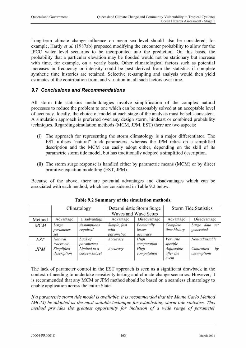
Queensland Government Queensland Climate Change and Community Vulnerability to Tropical CyclonesOcean Hazards Assessment - Stage 1
Long-term climate change influence on mean sea level should also be considered, forexample, Hardy et al. (1987ab) proposed modifying the encounter probability to allow for the IPCC water level scenarios to be incorporated into the prediction. On this basis, theprobability that a particular elevation may be flooded would not be stationary but increase with time, for example, on a yearly basis. Other climatological factors such as potential increases in frequency or intensity could be best derived from the statistics if completesynthetic time histories are retained. Selective re-sampling and analysis would then yield estimates of the contribution from, and variation in, all such factors over time.
9.7 Conclusions and Recommendations
All storm tide statistics methodologies involve simplification of the complex natural processes to reduce the problem to one which can be reasonably solved at an acceptable level of accuracy. Ideally, the choice of model at each stage of the analysis must be self-consistent.A simulation approach is preferred over any design storm, hindcast or combined probability techniques. Regarding simulation methods (MCM, JPM, EST) there are two aspects:
(i) The approach for representing the storm climatology is a major differentiator. TheEST utilises "natural" track parameters, whereas the JPM relies on a simplifieddescription and the MCM can easily adopt either, depending on the skill of its parametric storm tide model, but has traditionally adopted a simplified description.
(ii) The storm surge response is handled either by parametric means (MCM) or by direct primitive equation modelling (EST, JPM).
Because of the above, there are potential advantages and disadvantages which can be associated with each method, which are considered in Table 9.2 below.
Table 9.2 Summary of the simulation methods.
Climatology Deterministic Storm SurgeWaves and Wave Setup
Storm Tide Statistics
Method Advantage Disadvantage Advantage Disadvantage Advantage Disadvantage
MCM Largeparameter
set
Assumptionsrequired
Simple, fast with
parametric
Potentiallylesser
accuracy
Completetime history
Large data setgenerated
EST Natural
tracks etc
Lack of
parameters
Accuracy High
computation
Very site
specific
Non-adjustable
JPM Simplifieddescription
Limited to a chosen subset
Accuracy Highcomputation
Adjustableafter the
event
Controlled byassumptions
The lack of parameter control in the EST approach is seen as a significant drawback in thecontext of needing to undertake sensitivity testing and climate change scenarios. However, it is recommended that any MCM or JPM method should be based on a seamless climatology to enable application across the entire State.
If a parametric storm tide model is available, it is recommended that the Monte Carlo Method
(MCM) be adopted as the most suitable technique for establishing storm tide statistics. This
method provides the greatest opportunity for inclusion of a wide range of parameter
J0004-PR0001C 163 March 2001

Queensland Government Queensland Climate Change and Community Vulnerability to Tropical CyclonesOcean Hazards Assessment - Stage 1
sensitivities, including interseasonal, interdecadal and climate change impacts. Alternatively,
if a parametric model is not available, the Joint Probability Method (JPM) is favoured.
Finally, the adopted technique should automatically yield error or confidence limits in respect of the predictions. This can be done by accumulation of variance, analysis of variance (e.g.Twisdale et al. 1993) or use of sampling techniques such as the "bootstrap" (Prater et al.
1985; Hardy and Mason 1993).
9.8 References
Allen M.A. and Callaghan J. (2000) Extreme wave conditions for the south east Queenslandcoastal region. Environment Technical Report 32, Environmental Protection Agency, Qld.
Borgman L.E., Miller M.C., Butler H.L. and Reinhard R.D. (1992) Empirical simulation of future hurricane storm histories as a tool in engineering and economic analysis. Proc. Conf.Civil Engineering in the Oceans V, ASCE, 42-45.
Bretschneider C.L. (1967) Storm Surges. Advances in Hydroscience, 4, 341-414.
Casson E. and Coles S.G. (1998) Extreme hurricane wind speeds: estimation, extrapolation and spatial smoothing. Jnl Wind Engin and Industrial Aerodynamics, 74-76, 131-140.
Casson E. and Coles S.G. (2000) Spatial simulation of hurricane Events. Applied Statistics (toappear).
CERC (1966) Shore protection planning and design. Technical Report No. 4, US Army Corpsof Engineers, Coastal Engineering Research Centre. 3rd Ed, US Dept of the Army.
Coleman F. (1972) Frequencies, tracks and intensities of tropical cyclones in the Australian region, 1909 - 1969. Bureau of Meteorology, Meteorological Summary. July.
Dexter P.E. (1975) Computing extreme value statistics for cyclone generated surges. Proc 2nd
Aust Conf Coastal and Ocean Engin, IEAust. Apr. pp 200-206.
Dexter P.E., Trajer F.L. and Gordon B. (1977) Design cyclones and design surges. Proc. Hydrology Symposium, IEAust, Brisbane, June.
Georgiou P.N., Davenport A.G. and Vickery P.J. (1983) Design wind speeds in regions dominated by tropical cyclones. Jnl Wind Engineering and Industrial Aerodynamics, 13, 139-152.
Georgiou P.N. (1985) Design wind speeds in tropical-cyclone prone areas. PhD Thesis. The
University of Western Ontario, London, Sept.
Gomes L., and Vickery, B.J. (1976) On the prediction of tropical cyclone gust speeds along the Northern Australian Coast. Dept. of Civil Engineering, Univ. Sydney, Australia, ResearchReport No. R278, 1976.
Hardy T.A., Mason L.B., Young I.R., bin Mat H. and Stark K.P. (1987a) Frequency of cyclone induced water levels including the effect of mean sea level rise : Trinity Point. Dept
J0004-PR0001C 164 March 2001

Queensland Government Queensland Climate Change and Community Vulnerability to Tropical CyclonesOcean Hazards Assessment - Stage 1
of Civil and Systems Engin, James Cook University. Prep for Macdonald Wagner ConsultingEngineers. Oct.
Hardy T.A., Mason L.B., Young I.R., bin Mat H. and Stark K.P. (1987b) Frequency of cyclone induced water levels including the effect of mean sea level rise : Palm Cove. Dept of Civil and Systems Engin, James Cook University. Prep for Macdonald Wagner ConsultingEngineers. Oct.
Hardy T.A. and Mason L.B. (1993) Frequency of cyclone induced water levels: Cairns Casino site. Dept of Civil and Systems Engin, James Cook University. Prep for ConcreteConstructions Qld. Sep.
Harper B.A. Sobey R.J. and Stark K.P. (1977) Numerical simulation of tropical cyclone stormsurge along the Queensland coast - Parts I to X. Dept Civil and Systems Engin., James Cook
University, Nov.
Harper B.A. and Stark K.P. (1977) Probabilities of water levels at Townsville resulting fromthe combined effects of cyclone storm surge, tide and waves. Dept of Civil and SystemsEngin., James Cook University, Dec.
Harper B.A. (1983) Half Tide tug harbour extreme water level study. Report prepared by Blain Bremner and Williams Pty Ltd for DBCT-UDC Joint Venture. Sept.
Harper B.A. and McMonagle C.J. (1985) Storm tide statistics - methodology. Report prepared by Blain Bremner and Williams Pty Ltd for the Beach Protection Authority Queensland, Jan.
Harper B.A. (1985) Storm tide statistics - Parts 1 to 8. Reports prepared by Blain Bremner
and Williams Pty Ltd for the Beach Protection Authority Queensland, Jan.
Harper B.A. (1996a) Risk modelling of cyclone losses, Proc IEAust Annual Engin Conf, IEAust, Darwin, Ap, 53-88.
Harper B.A. (1996b) The application of numerical modelling in natural disaster risk management. Proc Conf on Natural Disaster Reduction NDR’96, Institution of Engineers
Australia, Gold Coast, Sep, 107-114, ISBN 0 85825 662 2.
Harper B.A. (1999a) Storm tide threat in Queensland: history, prediction and relative risks. Dept of Environment and Heritage, Conservation Tech Rep No. 10, RE 208, ISSN 1037-4701, Jan (2nd ed.).
Harper B.A. (1999b) Numerical modelling of extreme tropical cyclone winds. APSWESpecial Edition, Journal of Wind Engineering and Industrial Aerodynamics, 83, 35 - 47.
Ho F.P., Tracy R.J, Myers V. and Foat N.S. (1976) Storm tide frequency analysis for the open coast of Virginia, Maryland and Delaware. NOAA Technical Memorandum NWS HYDRO-32, Silver Spring.
Holland G.J. (1981) On the quality of the Australian tropical cyclone data base. Aust Met
Mag, Vol 29 No 4. Dec.
J0004-PR0001C 165 March 2001

Queensland Government Queensland Climate Change and Community Vulnerability to Tropical CyclonesOcean Hazards Assessment - Stage 1
Holthouse H. (1971) Cyclone. Rigby.
Irish J.L. (1976a) Report on storm tide levels for Pioneer River model study committee.Report prepared by Cameron McNamara and Partners. March.
Irish J.L. (1976b) Storm surge and flooding at Farnborough Beach. Report prepared byCameron McNamara and Partners for Iwasaki Sangyo Co (Australia) Pty Ltd, March.
Irish J.L. (1977) Surge and storm tide frequency estimation for coastal locations subject to cyclones. Proc 3rd Aust Conf Coastal and Ocean Engin. IEAust. Apr.
James M. and Mason L. (1999) Generation of a synthetic tropical cyclone database. Proc. 14th
Australasian Conf. Coastal and Ocean Engineering, IEAust, Perth, Apr, 407-412.
Jelesnianski C.P. (1965) A numerical calculation of storm tides induced by a tropical storm impinging on a continental shelf. Monthly Weather Review, 93, 343-358.
Jelesnianski C.P. (1972) SPLASH - special program to list amplitudes of surges from hurricanes - I landfall storms. NOAA Technical Memorandum NWS TDL-46.
Kepert J. and Wang Y. (2000) The dynamics of boundary layer jets within the tropical cyclone core - Part II: nonlinear enhancement. Jnl Atmospheric Sciences (to appear).
Lourensz R.S. (1977) Tropical cyclones in the Australian region July 1909 to June 1975. Bureau of Meteorology.
Lourensz R.S. (1981) Tropical cyclones in the Australian region July 1909 to June 1980. Bureau of Meteorology. Oct.
McMonagle C.J. (1979) Storm surge and tide investigations for new Brisbane Airport. Report prepared by Blain Bremner and Williams Pty Ltd for Commonwealth Dept Housing and Construction. Feb.
McMonagle C.J. (1980) Extreme water levels Gladstone and The Narrows. Report prep by Blain Bremner and Williams Pty Ltd for Coordinator General’s Dept, Queensland. Nov.
McMonagle C.J. (1995a) Numerical simulation of storm surge along the Queensland coast - Part XI Cardwell Region. Report prepared by Rust PPK Pty Ltd for The Beach Protection
Authority Queensland. Nov.
McMonagle C.J. (1995b) Storm tide statistics Cardwell region. Report prepared by Rust PPK Pty Ltd for The Beach Protection Authority Queensland, Oct.
Martin G.S. (1974) Probability distributions for hurricane wind gust speeds on the Australian coast. Proc. Conf. Applications of Probability Theory to Structural Design, IEAust,Melbourne, Australia, 1974, 55-56.
Mason L.B., Hardy T.A. and Bode L. (1992) Frequency of cyclone induced water levels - Marlin coast. Dept of Civil and Systems Engin, James Cook University. Prepared forMulgrave Shire Council.
J0004-PR0001C 166 March 2001
Queensland Government Queensland Climate Change and Community Vulnerability to Tropical CyclonesOcean Hazards Assessment - Stage 1
Nelson R.C. (1975) Tropical cyclone storm surges in Australia 1880 to 1970. Proc 2nd Aust Conf Coastal and Ocean Engin., IEAust.
Nickerson J.W. (1971) Storm surge forecasting. Navy Weather Research Facility, Tech Report 10-71.
Prater M.D., Hardy T.A., Butler H.L. and Borgman L.E. (1985) Estimating error of coastal stage frequency curves. Proc. 19th Intl. Conf. Coastal Engineering, ASCE, 162-172.
Russell, L.R. (1971) Probability distributions for hurricane effects. Jnl. Waterways, Harbors
and Coastal Eng. Div., ASCE., Paper 7886, February 1971.
Scheffner N.W., Borgman L.E. and Mark D.J. (1996) Empirical simulation technique based storm surge frequency analysis. Jnl Waterways, Port, Coastal and Ocean Eng., ASCE, 122, 2, 93-101.
Scheffner N.W. and Borgman L.E. (1996) The empirical simulation technique - a bootstrap-based life cycle approach to frequency analysis. Proc Stochastic Hydraulics'96. In: Tickle,Goulter, Xu, Wasimi and Bouchart (eds), 1996, Balkema, Rotterdam, ISBN 90 5410 817 7, 389-394.
Shapiro L.J. 91983) The asymmetric boundary layer flow under a translating hurricane. Jnl.
Atmospheric Science, AMS, 40(8), 1994-1998.
Silvester R. and Mitchell H.L. (1977) Storm surges around Australian coastlines. Proc 3rd
Aust Conf Coastal and Ocean Engin. IEAust. Melb. Apr.
Sobey R.J., Harper B.A. and Stark K.P. (1977) Numerical simulation of tropical cyclone storm surge along the Queensland coast. Research Bulletin CS14. Dept Civil and SystemsEngin. James Cook University, May.
Sobey R.J., Mitchell G.M. and Adil T.S. (1979) Trinity Inlet storm surge study. Report prepared by Dept Civil and Systems Engin James Cook University for Commonwealth Dept Housing and Construction.
Sobey R.J., Stark K.P. and Adil T.S. (1979) Weipa Peninsula extreme water level study. Report prepared by Dept of Civil and Systems Engin James Cook University for ComalcoLimited. Aug.
Stark K.P. (Ed.) (1972) Cyclone Althea - Part II storm surge and coastal effects. James Cook
University. Oct.
Stark K.P. (1976) Rosslyn Bay boat harbour surge investigation. Report prepared by Dept of Civil and Systems Engin James Cook University.
Stark K.P. (1979) Cairns storm surge plus tide levels. Report prepared by Dept of Civil and Systems Engin James Cook University for Cairns City Council. Dec.
J0004-PR0001C 167 March 2001

Queensland Government Queensland Climate Change and Community Vulnerability to Tropical CyclonesOcean Hazards Assessment - Stage 1
Trajer F.L. (1973) A manual storm surge forecasting scheme for the Australian tropics. 1st Aust Conf Coastal Engin, IEAust, Sydney, May, 215-220.
Treloar D.G. (1985) Storm tide statistics - Hervey Bay region. Report prepared by Lawson
and Treloar Pty Ltd for The Beach Protection Authority Queensland. Aug.
Twisdale L.A. and Vickery P.J. (1992) Predictive methods for hurricane winds in the United States - final report, SBIR Grant ISI 916035, National Science Foundation, Washington, DC,Sept.
Twisdale L.A., Vickery P.J. and Hardy M.B. (1993) Uncertainties in the prediction ofhurricane windspeeds. Proc. Symp. Hurricanes of 1992, ASCE, Miami, Dec, ISBN 0-7844-0046-6, 706-715.
US Weather Bureau (1968) Meteorological characteristics of the Probable MaximumHurricane, Atlantic and Gulf Coasts of the United States. Dept. of Commerce, Silver Spring, Md., Memo HUR 7-79 (unpublished).
Van Gelder P.H.A.J.M. (1996) A new statistical model for extreme water levels along the Dutch coast. Proc Stochastic Hydraulics'96. In: Tickle, Goulter, Xu, Wasimi and Bouchart (eds), 1996, Balkema, Rotterdam, ISBN 90 5410 817 7, 243-249.
Vickery P.J. and Twisdale L.A. (1994) Hurricane windspeeds at inland locations. Proc Structures Congress, ASCE, Apr.
Vickery P.J. and Twisdale L.A. (1995a) Prediction of hurricane wind speeds in the United States. J. Struct. Engin., 121(11), ASCE, 1691-1699.
Vickery P.J. and Twisdale L.A. (1995b) Wind-field and filling models for hurricane wind speed prediction. J. Struct. Engin., ASCE, 121(11), 1700-1709.
Ward E.G., Borgman L.E. and Cardone V.J. (1979) Statistics of hurricane waves in the Gulfof Mexico. Jnl Petroleum Engineering, 31, 5, 632-642.
Whittingham H.E. (1958) The Bathurst Bay hurricane and associated storm surge. Aust. Met.
Mag., 23, Dec.
Whittingham H.E. (1959) Storm surges along the Queensland coast. Aust Met. Mag., 27, 40-41.
Whittingham H.E. (1968) The “Douglas Mawson” tropical cyclone of 1923. In TropicalCyclones in the Northern Australian Regions for 1964-1965 Season, Appendix 1. Meteorological Summary. Bureau of Meteorology. Feb.
Wyland R.M. and Thornton E.B. (1991) Extremal wave statistics using three hindcasts. Jnl
Waterways, Port, Coastal and Ocean Engineering, ASCE, 117,1, 60-74
J0004-PR0001C 168 March 2001
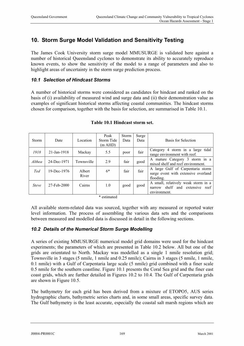
Queensland Government Queensland Climate Change and Community Vulnerability to Tropical CyclonesOcean Hazards Assessment - Stage 1
10. Storm Surge Model Validation and Sensitivity Testing
The James Cook University storm surge model MMUSURGE is validated here against a number of historical Queensland cyclones to demonstrate its ability to accurately reproduce known events, to show the sensitivity of the model to a range of parameters and also to highlight areas of uncertainty in the storm surge prediction process.
10.1 Selection of Hindcast Storms
A number of historical storms were considered as candidates for hindcast and ranked on thebasis of (i) availability of measured wind and surge data and (ii) their demonstration value as examples of significant historical storms affecting coastal communities. The hindcast stormschosen for comparison, together with the basis for selection, are summarised in Table 10.1.
Table 10.1 Hindcast storm set.
Storm Date LocationPeak
Storm Tide(m AHD)
StormData
SurgeData Basis for Selection
1918 21-Jan-1918 Mackay 5.5 poor fairCategory 4 storm in a large tidalrange environment with reef.
Althea 24-Dec-1971 Townsville 2.9 fair goodA mature Category 3 storm in a mixed shelf and reef environment.
Ted 19-Dec-1976 AlbertRiver
6* fair fairA large Gulf of Carpentaria stormsurge event with extensive overlandflooding.
Steve 27-Feb-2000 Cairns 1.0 good goodA small, relatively weak storm in anarrow shelf and extensive reefenvironment.
* estimated
All available storm-related data was sourced, together with any measured or reported water level information. The process of assembling the various data sets and the comparisonsbetween measured and modelled data is discussed in detail in the following sections.
10.2 Details of the Numerical Storm Surge Modelling
A series of existing MMUSURGE numerical model grid domains were used for the hindcastexperiments; the parameters of which are presented in Table 10.2 below. All but one of the grids are orientated to North. Mackay was modelled as a single 1 nmile resolution grid;Townsville in 3 stages (5 nmile, 1 nmile and 0.25 nmile); Cairns in 3 stages (5 nmile, 1 nmile,0.1 nmile) with a Gulf of Carpentaria large scale (5 nmile) grid combined with a finer scale0.5 nmile for the southern coastline. Figure 10.1 presents the Coral Sea grid and the finer eastcoast grids, which are further detailed in Figures 10.2 to 10.4. The Gulf of Carpentaria grids are shown in Figure 10.5.
The bathymetry for each grid has been derived from a mixture of ETOPO5, AUS series hydrographic charts, bathymetric series charts and, in some small areas, specific survey data. The Gulf bathymetry is the least accurate, especially the coastal salt marsh regions which are
J0004-PR0001C 169 March 2001
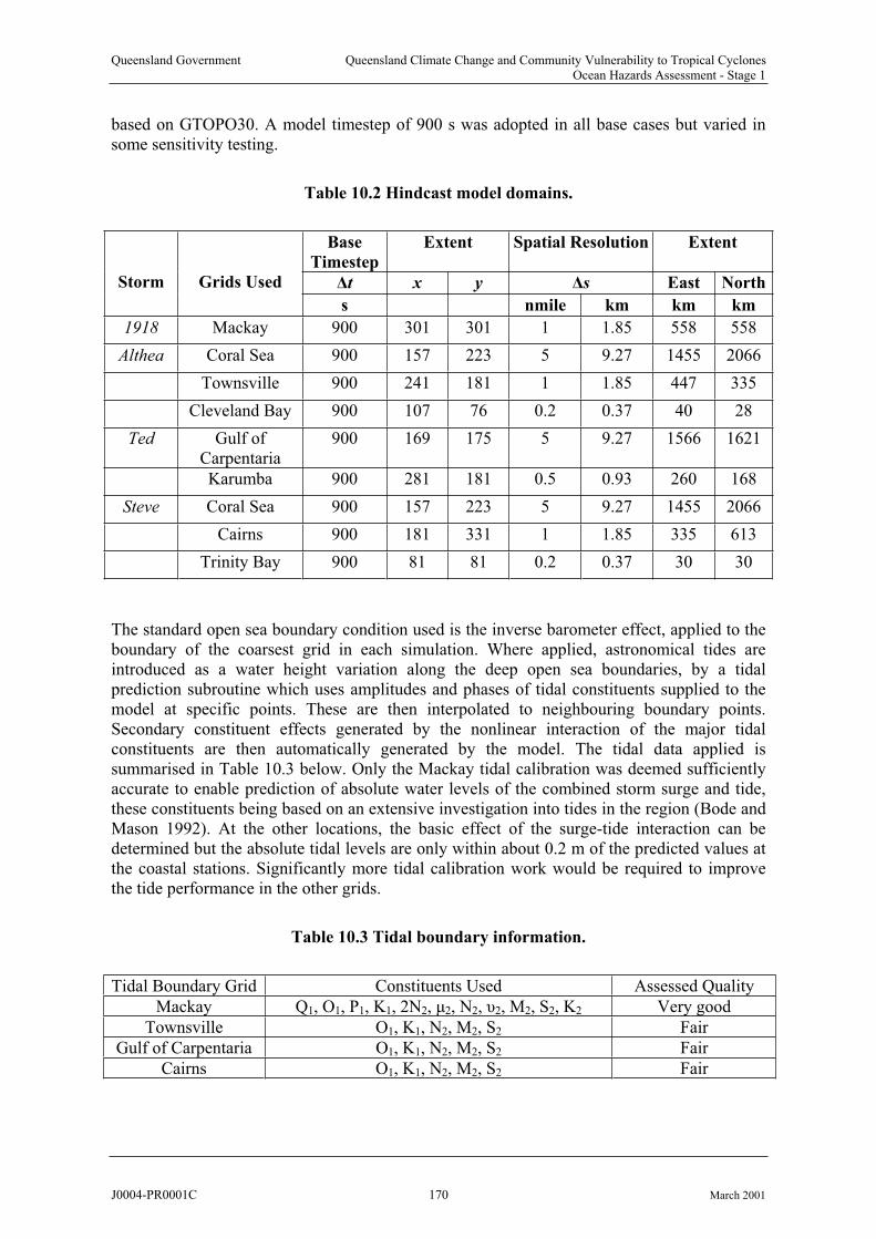
Queensland Government Queensland Climate Change and Community Vulnerability to Tropical CyclonesOcean Hazards Assessment - Stage 1
based on GTOPO30. A model timestep of 900 s was adopted in all base cases but varied in some sensitivity testing.
Table 10.2 Hindcast model domains.
Base
Timestep
Extent Spatial Resolution Extent
t x y s East NorthStorm Grids Used
s nmile km km km
1918 Mackay 900 301 301 1 1.85 558 558
Althea Coral Sea 900 157 223 5 9.27 1455 2066
Townsville 900 241 181 1 1.85 447 335
Cleveland Bay 900 107 76 0.2 0.37 40 28
Ted Gulf of Carpentaria
900 169 175 5 9.27 1566 1621
Karumba 900 281 181 0.5 0.93 260
Steve Coral Sea 900 157 223 5 9.27 1455 2066
Cairns 900 181 331 1 1.85 335 613
Trinity Bay 900 81 81 0.2 0.37 30 30
168
The standard open sea boundary condition used is the inverse barometer effect, applied to the boundary of the coarsest grid in each simulation. Where applied, astronomical tides are introduced as a water height variation along the deep open sea boundaries, by a tidal prediction subroutine which uses amplitudes and phases of tidal constituents supplied to themodel at specific points. These are then interpolated to neighbouring boundary points. Secondary constituent effects generated by the nonlinear interaction of the major tidal constituents are then automatically generated by the model. The tidal data applied issummarised in Table 10.3 below. Only the Mackay tidal calibration was deemed sufficiently accurate to enable prediction of absolute water levels of the combined storm surge and tide,these constituents being based on an extensive investigation into tides in the region (Bode andMason 1992). At the other locations, the basic effect of the surge-tide interaction can be determined but the absolute tidal levels are only within about 0.2 m of the predicted values at the coastal stations. Significantly more tidal calibration work would be required to improve the tide performance in the other grids.
Table 10.3 Tidal boundary information.
Tidal Boundary Grid Constituents Used Assessed Quality
Mackay Q1, O1, P1, K1, 2N2, µ2, N2, 2, M2, S2, K2 Very good
Townsville O1, K1, N2, M2, S2 Fair
Gulf of Carpentaria O1, K1, N2, M2, S2 Fair
Cairns O1, K1, N2, M2, S2 Fair
J0004-PR0001C 170 March 2001

Queensland Government Queensland Climate Change and Community Vulnerability to Tropical CyclonesOcean Hazards Assessment - Stage 1
All hindcasts have used a common sea bed roughness height z0=0.001 m (giving a roughness
length 0.027 m) and Cd=(vk/(z1/z0))2 , where vk is Von Karman's constant and z1 is half the
water depth in the 2D model.
The model was run in 2D (depth-integrated) mode for all hindcasts. Limited 3D simulations were undertaken of cyclone Althea, where 5 sigma levels were run in conjunction with a turbulence closure model which calculates turbulent kinetic energy and turbulent length scales. These are then used to determine the vertical eddy viscosity parameters for the momentum model.
The following matrix summarises the range of sensitivity tests undertaken in conjunction with the hindcast experiments.
Table 10.4 Model sensitivity tests undertaken.
Region: Mackay Townsville Gulf Cairns
Storm: 1918 Althea Ted Steve
Sensitivity Test Case
5 X X XResolution 1 X X X
(nmile) 0.5 X0.2 X X
300 XTimestep 900 X X X X
(s) 1800 X
Dimension 2D X X X X3D X
Tide Tide Only X X X XWith Tide X X X XNo Tide X X X X
Wetting Dry X X X XWet X
Reef Reef X X XNo Reef X X X
Nonlinear Yes X X X XAdvection No X
J0004-PR0001C 171 March 2001

Queensland Government Queensland Climate Change and Community Vulnerability to Tropical CyclonesOcean Hazards Assessment - Stage 1
Figure 10.1 Overview of Coral Sea hindcast grids.
J0004-PR0001C 172 March 2001
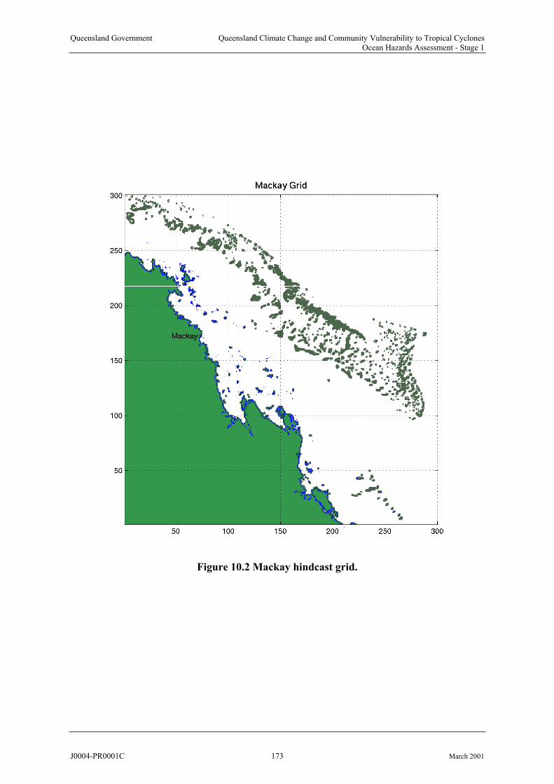
Queensland Government Queensland Climate Change and Community Vulnerability to Tropical CyclonesOcean Hazards Assessment - Stage 1
Figure 10.2 Mackay hindcast grid.
J0004-PR0001C 173 March 2001

Queensland Government Queensland Climate Change and Community Vulnerability to Tropical CyclonesOcean Hazards Assessment - Stage 1
Figure 10.3 Townsville hindcast grids.
J0004-PR0001C 174 March 2001
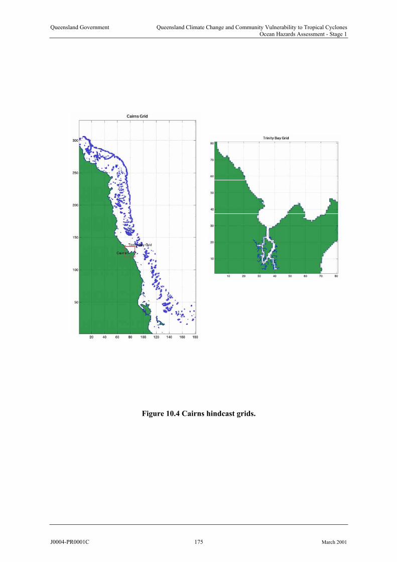
Queensland Government Queensland Climate Change and Community Vulnerability to Tropical CyclonesOcean Hazards Assessment - Stage 1
Figure 10.4 Cairns hindcast grids.
J0004-PR0001C 175 March 2001
Queensland Government Queensland Climate Change and Community Vulnerability to Tropical CyclonesOcean Hazards Assessment - Stage 1
Figure 10.5 Gulf of Carpentaria hindcast grids.
J0004-PR0001C 176 March 2001

Queensland Government Queensland Climate Change and Community Vulnerability to Tropical CyclonesOcean Hazards Assessment - Stage 1
10.3 The January 1918 Cyclone at Mackay
This event remains one of the most significant examples of the inundation of an Australian community by an extreme storm tide. However, due to the lack of widespread instrumentationof winds and water levels at that time, many specific details about the track and intensity ofthe storm and the actual water levels attained remain clouded. It is certain that a very intense cyclone crossed the coast to the north of Mackay on the morning of Monday 21st January 1918. A storm surge inundated the town and nearby beaches at about the same time. As aresult of the heavy rain, the river subsequently again flooded the town on the following day. The following reconstruction of the event is based on information gained from only a few key sources but taken together these facts form a compelling and likely scenario of events. A detailed account in Bath (1957) attributed to the Harbour Master states that 14 bodies had been recovered by the 23rd January, with three vessels sunk, another three ashore and all wharves collapsed. The Daily Mercury of 28th January reported 20 deaths at that time and Visher and Hodge (1925) records that 30 lives were lost in total.
10.3.1 Available Tropical Cyclone Data
The National Climate Centre official track for this event is scant, essentially based on that ofLourensz (1981) which is probably derived from Bath (1957), at least in part. However, theNCC and Lourensz tracks share an error in the time of landfall which incorrectly has thestorm making landfall on the 20th rather than the 21st (EST). This error was also noted by Gourlay and Hacker (1986) who point to the extensive account of events in the Mackay Daily
Mercury newspaper report of 26th January. The earliest official assessment of the meteorology appears to be that by Bath (1957), who quotes extensively from the log of theLightkeeper of Flat Top Island, a Captain G. F. Long. The Lightkeeper noted some pressure values and estimated wind speed variously throughout the storm whilst endeavouring to provide shelter to his family. Bath also provides the Post Office barograph and mentionsreports by the Postmaster and a private observer - Mr T. (sic) Croker (refer later). The Daily Mercury (1918) also mentions a number of observations of atmospheric pressure made by aMr P. Armati during the passage of the cyclone and some regional pressures are available from the Brisbane Courier Mail (Callaghan 2000). No direct wind speed measurements areavailable for the event but there are a number of pressure data as well as some observations of wind directional changes. Although the Daily Mercury (1918) contains extensive accounts of damage and personal hardships throughout the region, no eyewitnesses speak of experiencing the absolute calm of the eye. However, the later special historical feature (Daily Mercury1993) does refer to the community experiencing a lull between 7 am and 8 am. It is considered possible that this comment has been "loosely inferred" from an eyewitness account elsewhere in the same issue by a Mr Andrew Fordyce and that the town did not experience a true eye effect. Mr Fordyce was at the Richmond Mill Plantation at the time, which was about 8 km NNW of the town. During the course of this investigation, a letter from the Crokerfamily was provided which described a calm of about half an hour at Eimeo. Bath also reports that T. (sic) Croker reported a "sudden lull and the wind soon came from the north". His pressure measurement of 27.54"Hg (932.6 hPa) at about 0730 EST 21/1 (2230 UTC 20/1) is accepted by Bath as the lowest reading made during the event. Another measurement of 27.55"Hg is reported in the Daily Mercury (1993) as being due to the Harbour Master Captain Greenfield but this may simply be repeating the Croker value.
J0004-PR0001C 177 March 2001

Queensland Government Queensland Climate Change and Community Vulnerability to Tropical CyclonesOcean Hazards Assessment - Stage 1
10.3.2 Available Storm Tide Data
There was no automatic tide recording system in operation at Mackay in 1918 and, although a number of tide boards were probably in existence along the river port area, all would have been inundated during the event. This is confirmed by Parkinson et al. (1950) which mentionsthat a visual marker system was first made available in 1928 near Flat Top Island and an automatic recording system at the Outer Harbour in 1939. Some timing and relative water level elevation data during the storm tide can be inferred from the Lightkeeper's account in Bath and from the Daily Mercury reports. The newspaper details the experiences of a numberof individuals who were impacted by the storm tide both within the town and along the nearby coast. Some personal statements were also made available from survivors of the event that had been obtained during earlier historical investigations into flooding in the Pioneer River (Gourlay, pers. comm.). Based on all of the reports it is clear that the storm tide reachedupriver to approximately the position of the Customs House located on the riverbank at thecorner of Sydney St and River St (formerly North St). This is also the position of the ForganBridge. The most definitive peak water level value is first mentioned in a State Governmentreport to Parliament (Harbours and Rivers Department 1918). The report states that the seasurface "slowly rose for about an hour, reaching a height of 7 feet 9 inches above highest
spring-tide level; it remained stationary at that height for about 10 minutes, and slowly fell again". Besides the above, there is no specific detail provided of the event. Parkinson et al.
(1950) is the next available reference - which states that sea water rose "approximately 8ft
above high water level", thus according with the earlier value. However, neither reference allows recovery of a specific level without knowledge of the actual tide datum beingreferenced. Although the Parkinson report focuses particularly on river flooding it does include a map (Plan No. 14) which indicates the extent of seawater inundation during the 1918 event. This is reproduced in Figure 10.6 courtesy of AGSO (Granger, pers. comm.)where the original map has been digitised and the locations of known deaths due to drowning have been marked by AGSO.
This inundation line is shown as being slightly above the 17 ft ground contour on State Datum in the vicinity of the Customs House. Converting 17 ft to AHD yields a level of 5.35 m,which has been variously quoted as the actual peak level for the event. Unfortunately Parkinson does not quote a specific level and no description of exactly how the map levels were obtained is provided. It can only be assumed that all of the Daily Mercury reports wereavailable and that the Harbour and Rivers Department level was used in some way. Indeed, the Daily Mercury and other eyewitness reports are certainly broadly consistent with this map.Work by Gourlay and Hacker (1986) however, is able to shed some light on the likely "highest spring-tide level" datum quoted by Harbour and Rivers, whereby a Standard High
Water Level (SHWL) was used on charts from 1886 to 1930. This level, peculiar to Mackay, is now known to be 3.14 m AHD. Adding the 7 feet 9 inches to this level yields 5.50 m AHD (or 5.33 m on the old State Datum, being 17.5 ft). Accordingly, it is determined that 5.5 mAHD should be regarded as the highest inundation level due to the storm tide. This puts muchreliance on the admittedly brief but vivid description given in the Harbour and Rivers report.However, it also acknowledges that this was reported and published in the actual year of the event and stated with some certainty by a technical source charged with the maintenance andnavigation of the port. It is also likely that the closeness of the peak level to the CustomsHouse benchmark probably greatly assisted in the recovery of such a level during the confusion of the disaster. For example, the consequent river flood two days later reached a slightly higher level (Gourlay and Hacker 1986), thus obliterating the storm tide debris lines.
J0004-PR0001C 178 March 2001

Queensland Government Queensland Climate Change and Community Vulnerability to Tropical CyclonesOcean Hazards Assessment - Stage 1
The map by Parkinson remains as probably the most comprehensive record of the inundation by the storm tide but should be taken with an official peak level of 5.50 m AHD.
Town
Beach
Pioneer
River
South Sydney St
(Mrs Daly)
0 1 km
Post Office
J Croker
Figure 10.6 Extent of inundation due to the storm tide during Mackay 1918
(after Parkinson 1950, and AGSO 2000)
It should be noted that the Queensland Regional Office of the Bureau of Meteorology has in its archive a hand-drawn facsimile of the water level trace during the event together with thepredicted tide. Clearly no such record existed and it is concluded that this was created to provide an illustration at some time to match the quoted 5.35 m peak level (possibly byHerbert Wittingham).
Taking all of the above into consideration, Figure 10.7 summarises the available data in regard to the magnitude and timing of the 1918 storm tide at Mackay. The predicted high tide on the morning of 21st January was 1.98 m AHD at 0630 EST (Broadbent 2000). The peak level of 5.5 m is shown nominally occurring at 7 am EST (2100 UTC) which is consistent with eyewitness accounts from the Daily Mercury (1918, 1993) where it was variously reported that the surge arrived quickly (in the town) at about 5 am (1900 UTC) and subsided about 9 am (2300 UTC). This may be assumed the approximate period where the water levels exceeded HAT, at which point some properties would have experienced initial flooding. The7 am peak timing is also consistent with the Harbour and Rivers report of "slowly rising over
an hour" if taken relative to exceeding HAT. Another report, apparently closer to the beach,tells of a "wall of water" at approximately 5 am (1900 UTC). Either way, the peak storm tidelevel apparently occurred close to the time of peak predicted tide, yielding a storm surge pluswave setup component of approximately 3.5 m. Eyewitness reports also described large waves ("rollers") within the town with heights of the order of 2.5 m to 3 m. Certainly this would have been possible in some areas since the depth of inundation above HAT was about 2 m. A number of houses were displaced from their piers and either destroyed or floated somedistance from their property and the wave related debris was significant. Interestingly,
J0004-PR0001C 179 March 2001
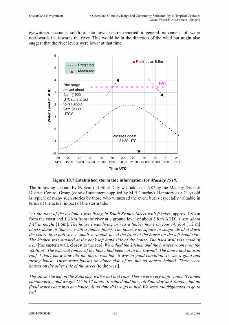
Queensland Government Queensland Climate Change and Community Vulnerability to Tropical CyclonesOcean Hazards Assessment - Stage 1
eyewitness accounts south of the town centre reported a general movement of water northwards i.e. towards the river. This would be in the direction of the wind but might also suggest that the river levels were lower at that time.
-2
-1
0
1
2
3
4
5
6
20
14:00
20
15:00
20
16:00
20
17:00
20
18:00
20
19:00
20
20:00
20
21:00
20
22:00
20
23:00
21
00:00
21
01:00
Time UTC
Wate
r L
evel
m A
HD
Predicted
Measured
HAT"the surge
arrived about
5am (1900
UTC)… started
to fall about
9am (2300
UTC)"
crosses coast
21:30 UTC
Peak Level 5.5m
Figure 10.7 Established storm tide information for Mackay 1918.
The following account by 89 year old Ethel Daly was taken in 1987 by the Mackay Disaster District Control Group (copy of statement supplied by M.R.Gourlay). Her story as a 21 yr old is typical of many such stories by those who witnessed the event but is especially valuable interms of the actual impact of the storm tide:
"At the time of the cyclone I was living in South-Sydney Street with friends [approx 1.8 kmfrom the coast and 1.3 km from the river at a ground level of about 3.8 m AHD]. I was about
5'4" in height [1.6m]. The house I was living in was a timber home on four (4) foot [1.2 m] blocks made of timber...(with a timber floor). The house was square in shape, divided down
the centre by a hallway. A small verandah faced the front of the house on the left hand side.
The kitchen was situated at the back left hand side of the house. The back wall was made of iron [the eastern wall, closest to the sea]. We called the kitchen and the harness room area the
'Skillion'. The external timber of the home had been cut in the sawmill. The house had an iron
roof. I don't know how old the house was but it was in good condition. It was a good and
strong house. There were houses on either side of us, but no houses behind. There were houses on the other side of the street [to the west].
The storm started on the Saturday, with wind and rain. There were very high winds. It rained
continuously, and we got 12" in 12 hours. It rained and blew all Saturday and Sunday, but no
flood water came into our house. At no time did we go to bed. We were too frightened to go to
bed.
J0004-PR0001C 180 March 2001

Queensland Government Queensland Climate Change and Community Vulnerability to Tropical CyclonesOcean Hazards Assessment - Stage 1
At about 1am on Monday morning, the next door neighbours, Mrs Dwyer and three children,
came knocking at our door. Their house had collapsed under the force of the wind and the
rain. At that point in time there was no major flooding. We made them comfortable and gave
them some dry clothes. I made a cup of tea on a primus.
A large piece of timber was blown through the window in the harness room. Bob was holding
a cushion from the sulky up against the window trying to stop the rain from coming in.
At about 6.30am on Monday morning I had just finished putting the primus away, and called
Bob to come in to us. He came in, and we were all in the dining room.
At that point in time, the back of the house collapsed. The noise sounded like a bomb going
off. The entire back wall and the roof had fallen in. Straight away salt water was all around
us and inside the house. The collapsed skillion effectively blocked the water from coming in,
and water could only come in quickly through the front of the house.
Within seconds the salt water was up to my shoulders in the house. I went straight to the front
of the house to try to throw some furniture back into the front door to stop all the furniture from going out through the front door. I was standing near the front door (and) wedged
myself against the door to stop from being washed outside the house. I looked around and
saw Mr Lemberg's house collapse and be washed away. Mr and Mrs Harry Kenny's house on
the left of our house was washed off the blocks and across the road. The house spun around
and landed on Mr McIvor's fence across the road. Mr and Mrs Kenny were still in the house
at the time. The Kenny's had to swim from their house to the steps of the McIvor's house.
The Potter's house was washed off its high blocks. It was spun around and ended up facing
the other way towards Juliet Street. I actually saw this occur from the front door.
As I was looking out the door I could see big rollers, just like the open ocean. The waves were about 8 or 9 feet high [2.6 m; local depth estimated as about 2 m at the time] and were just
like the surf at the beach. If I had been out in the street the waves would have been over my
head. I was a competent swimmer in those days, but I believe that I could not have swum
across the street.
Inside our house two women and four children sat on the tables, and Bob and I stood in the
water for the next five and half hours. In this time the water was all salt water. It took five and
a half hours for the water to drop below the floorboards. We then went across the road to Mr
Mincher's house and they looked after us. As we walked across the road the water was up to my waist [0.8 m].
The back of our house faced east towards Town Beach. The houses that were washed off their
blocks were washed away from the Town Beach direction. There were no houses directly
behind us which could have stopped some of the force of the wave. The rollers which I saw
were going up Sydney Street in the direction of the river. Mattresses, animals, birds, all sorts
of things, were floating up Sydney Street also towards the river."
J0004-PR0001C 181 March 2001

Queensland Government Queensland Climate Change and Community Vulnerability to Tropical CyclonesOcean Hazards Assessment - Stage 1
10.3.3 Reconstruction of the Event
The following describes the methodology adopted in developing a consistent description of the storm parameters. It relies on the available data combined with theoretical spatial andtemporal variations in wind and pressure as predicted by an analytical model (Harper andHolland 1999), detailed in Appendix C. The model was systematically adjusted for reasonable values of the key parameters such as track, central pressure and radius to maximum winds. The available information was then compared with the model output to determine the validityof the various assumptions. Consistent with experience from cyclone Althea (refer Section
10.4), a windfield asymmetry based on a max of 115º was subsequently found to represent the best fit to wind and storm surge results.
10.3.3.1 Synoptic Situation
As reported by Bath (1957), significant Coral Sea activity was noted about 18th January. Figure 10.8 presents Bath's MSL charts for the region for the 20th and 21st, showing the extensive low-pressure development. Ambient surrounding pressure is indicated asapproximately 29.75"Hg or 1007 hPa (the summer average) and this value has been used in the present assessment.
Figure 10.8 Mackay 1918 synoptic development (after Bath 1957).
J0004-PR0001C 182 March 2001
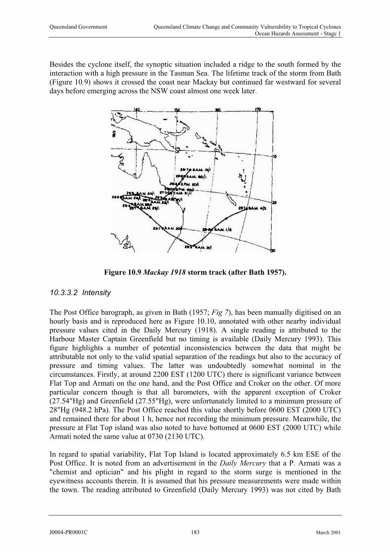
Queensland Government Queensland Climate Change and Community Vulnerability to Tropical CyclonesOcean Hazards Assessment - Stage 1
Besides the cyclone itself, the synoptic situation included a ridge to the south formed by the interaction with a high pressure in the Tasman Sea. The lifetime track of the storm from Bath (Figure 10.9) shows it crossed the coast near Mackay but continued far westward for severaldays before emerging across the NSW coast almost one week later.
Figure 10.9 Mackay 1918 storm track (after Bath 1957).
10.3.3.2 Intensity
The Post Office barograph, as given in Bath (1957; Fig 7), has been manually digitised on an hourly basis and is reproduced here as Figure 10.10, annotated with other nearby individual pressure values cited in the Daily Mercury (1918). A single reading is attributed to the Harbour Master Captain Greenfield but no timing is available (Daily Mercury 1993). This figure highlights a number of potential inconsistencies between the data that might be attributable not only to the valid spatial separation of the readings but also to the accuracy of pressure and timing values. The latter was undoubtedly somewhat nominal in the circumstances. Firstly, at around 2200 EST (1200 UTC) there is significant variance between Flat Top and Armati on the one hand, and the Post Office and Croker on the other. Of more particular concern though is that all barometers, with the apparent exception of Croker(27.54"Hg) and Greenfield (27.55"Hg), were unfortunately limited to a minimum pressure of 28"Hg (948.2 hPa). The Post Office reached this value shortly before 0600 EST (2000 UTC)and remained there for about 1 h, hence not recording the minimum pressure. Meanwhile, thepressure at Flat Top island was also noted to have bottomed at 0600 EST (2000 UTC) while Armati noted the same value at 0730 (2130 UTC).
In regard to spatial variability, Flat Top Island is located approximately 6.5 km ESE of thePost Office. It is noted from an advertisement in the Daily Mercury that a P. Armati was a"chemist and optician" and his plight in regard to the storm surge is mentioned in the eyewitness accounts therein. It is assumed that his pressure measurements were made within the town. The reading attributed to Greenfield (Daily Mercury 1993) was not cited by Bath
J0004-PR0001C 183 March 2001
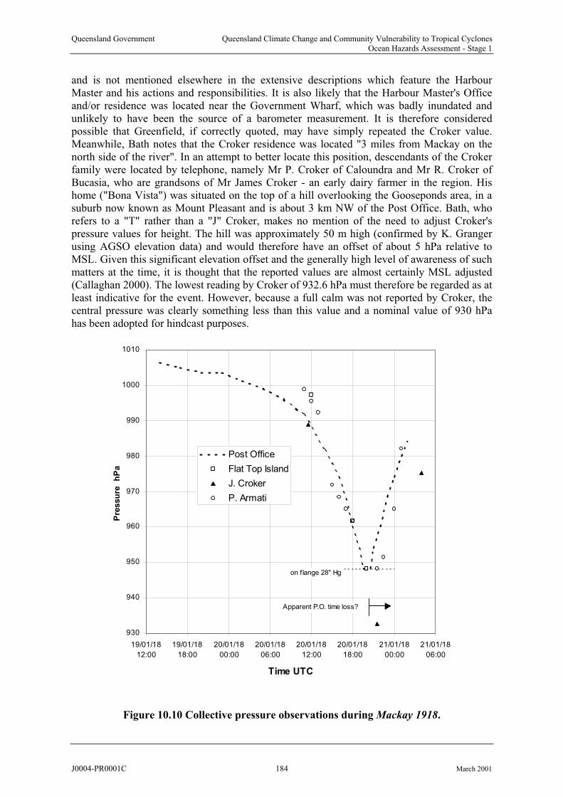
Queensland Government Queensland Climate Change and Community Vulnerability to Tropical CyclonesOcean Hazards Assessment - Stage 1
and is not mentioned elsewhere in the extensive descriptions which feature the Harbour Master and his actions and responsibilities. It is also likely that the Harbour Master's Office and/or residence was located near the Government Wharf, which was badly inundated and unlikely to have been the source of a barometer measurement. It is therefore consideredpossible that Greenfield, if correctly quoted, may have simply repeated the Croker value. Meanwhile, Bath notes that the Croker residence was located "3 miles from Mackay on thenorth side of the river". In an attempt to better locate this position, descendants of the Crokerfamily were located by telephone, namely Mr P. Croker of Caloundra and Mr R. Croker of Bucasia, who are grandsons of Mr James Croker - an early dairy farmer in the region. His home ("Bona Vista") was situated on the top of a hill overlooking the Gooseponds area, in asuburb now known as Mount Pleasant and is about 3 km NW of the Post Office. Bath, who refers to a "T" rather than a "J" Croker, makes no mention of the need to adjust Croker'spressure values for height. The hill was approximately 50 m high (confirmed by K. Granger using AGSO elevation data) and would therefore have an offset of about 5 hPa relative to MSL. Given this significant elevation offset and the generally high level of awareness of such matters at the time, it is thought that the reported values are almost certainly MSL adjusted (Callaghan 2000). The lowest reading by Croker of 932.6 hPa must therefore be regarded as at least indicative for the event. However, because a full calm was not reported by Croker, thecentral pressure was clearly something less than this value and a nominal value of 930 hPa has been adopted for hindcast purposes.
930
940
950
960
970
980
990
1000
1010
19/01/18
12:00
19/01/18
18:00
20/01/18
00:00
20/01/18
06:00
20/01/18
12:00
20/01/18
18:00
21/01/18
00:00
21/01/18
06:00
Time UTC
Pre
ssu
reh
Pa
Post Office
Flat Top Island
J. Croker
P. Armati
on f lange 28" Hg
Apparent P.O. time loss?
Figure 10.10 Collective pressure observations during Mackay 1918.
J0004-PR0001C 184 March 2001
Queensland Government Queensland Climate Change and Community Vulnerability to Tropical CyclonesOcean Hazards Assessment - Stage 1
10.3.3.3 Timing
The likely timing of the passage of the storm was addressed next. Besides the gross error inthe NCC track, no detail was available between a 2300 UTC fix of the storm on the (as corrected) 19th and the first overland fix 1 day later. Davidson et al. (1993) corrected the timing error and put the position at 0000 UTC 20/1 near 18.3ºS 152ºE with a constant track and speed to the coast, with the next position approx 30km inland at 21ºS 149ºE exactly 24 h later at 0000UTC 21/1. Taking a combination of the Davidson et al. and NCC starting points gave a nominal 0000 UTC 20/1 fix at 18.5ºS 152ºE, which is slightly to the south of Bath'strack. The timing of the close approach was then assessed based on a combination of the pressure readings from the various sites and also the observed changes in wind direction at Flat Top Island and by Croker (when noting a "sudden lull"). The Davidson et al. inland fix was then brought forward 1.5 h to apply at 2230 UTC on the previous day rather than 0000 UTC.
The Post Office barograph timing was discounted because the pen settled on the instrumentflange shortly before 0600 EST (2000 UTC) and there is an apparent timing error on the rising trace when compared with the 0730 EST (2330 UTC) Flat Top reading and also Armati's manual observations. It is considered possible (Callaghan 2000) that the instrumentrotation was actually slowed by the pen resting on the flange and resulted in an apparent timegain on the rising trace, leading to the perception that the minimum pressure occurred earlier than at the other sites.
10.3.3.4 Distance
Clearly, the storm passed quite close to Mackay and on the northern side. Mr Peter Croker of Caloundra was able to quote from a letter written by his mother-to-be who was with a party staying at the Eimeo Hotel and, as reported in the Daily Mercury (1918), walked to "Bona Vista" later that day. In her letter, she described a calm of about half an hour at Eimeo. TheDaily Mercury (1993) report by Fordyce indicates his experiencing a full calm at RichmondMill Plantation that ended around 9 or 10 am, but no duration was given. Some guidance is also provided by noting that there were no other reports in the Daily Mercury (1918) of experiencing an eye from any of the other isolated small coastal settlements such as Slade Point or Blacks Beach. Moreover, these sites reported experiencing significant surge effects,suggesting a coastal crossing somewhere still further to the north, but apparently not as far as Seaforth, where another party of eyewitnesses not reporting a calm were situated. As a resultof various sensitivity tests, a nominal +0.1 deg latitude shift was made to the Davidson et al.
(1993) initial land fix. This resulted in a closest approach to the Mackay Post Office of 23 kmat 2100 UTC 20/1, essentially being the time of landfall near Sand Bay, a sparsely settled area which is about 10 km west (and slightly north) of Shoal Pt. The full passage of the calm would have been about 1 h, making the Eimeo report consistent with being towards the southern edge of the eyewall and the Croker "sudden lull" consistent with clipping the southern edge only. On this basis, the model predicts that Seaforth might have experienced a similar lull to Eimeo and Richmond Mill Plantation may have had a longer lull because of the reduced inland winds, but not necessarily a complete calm. This is slightly at odds with the Richmond Mill account of a full calm which was apparently long enough to permit having breakfast, but the local wooded terrain may have contributes to lower wind speeds. Why someof the more inland communities such as Hatton did not report experiencing a calm still remains a mystery, but reports may have been suppressed by the sheer level of devastation suffered and a public lack of understanding of the structure of tropical cyclones.
J0004-PR0001C 185 March 2001

Queensland Government Queensland Climate Change and Community Vulnerability to Tropical CyclonesOcean Hazards Assessment - Stage 1
10.3.3.5 Phasing
As noted earlier, little guidance was available in regard to the storm track as it approached the coast. Initial trials using a single offshore fix and a single onshore fix provided consistency amongst the various pressure measurement sites only at the time of closest approach. At other times, difficulties were experienced in matching the shape of the pressure trace, especially inmatching the initial depression and then also the rapid descent to the minimum. One of themain difficulties appeared to be that the simple 2-point track placed the storm centre too far offshore about 12 h before landfall. Based on trial and error, an intermediate fix was then
devised which placed the centre at 20 S 150.2 E at 1100 UTC on 20/1, still on a straightline approach but approximately 3.5 h earlier than the 2-point fix track. This provided a better fit to the early stages and provided greater scope for a steeper pressure profile near the eye.
10.3.3.6 Radius to Maximum Winds and Wind Profile Peakedness
The Holland analytical wind and pressure model uses a radius to maximum wind (R) and a wind profile peakedness parameter (B) to spatially vary wind speed, direction and pressure at any point relative to a storm centre. Based on the foregoing assessment of peak intensity, timing and closest approach, various combinations of R and B (or rather B0, refer Appendix C) were systematically trialed and comparisons were made with the data. These changes werenot made in isolation but rather integrally with the foregoing assessments and, based on this approach, an R of 40 km and a B0 of 7.4 (B of 1.6) were selected as a reasonable compromisebetween peak error and bias error amongst the various sites, allowing for the "bottoming out" of several readings. This produced a relatively steep wind profile that is generally consistentwith the visually observed winds at Flat Top Island.
10.3.3.7 Final Track Parameters
Table 10.5 summarises the final storm parameters, while Figure 10.11 shows the track and predicted wind and pressure field as the storm made landfall. Note that there is little benefit in assuming the storm was changing its central pressure or its radius on approach to shore and there is no supporting information either way. Given the extent of the synoptic feature it is likely that the storm was relatively mature during this phase. Maintaining the pressure afterlandfall is less supportable but is retained here on the basis that emphasis is on the prediction of the storm surge. Many reports also suggest that the highest winds were experienced from the north and north-east, i.e after landfall. With max of 115º the analytical model does lend support to these observations, although the increased winds may equally have been caused by coastal convergence effects. Alternatively, this observation may have in part been due to a sudden increase in damage as a result of the wind direction having changed - it is likely that many buildings had "strain hardened" against the earlier wind direction but then were attackedfrom the other quadrant.
Table 10.5 Adopted hindcast parameters for the January 1918 cyclone.
Track Fix Speed Bearing CentralPressure
Radius Peakedness
Time Lat Long Vfm fm p0 R B0
UTC m s-1 hPa km
20/01/1918 00:00 18.0 152.5 6.4 228 930 40 7.4
20/01/1918 11:00 20.0 152.2 4.4 228 930 40 7.4
20/01/1918 22:30 21.1 148.9 8.1 228 930 40 7.4
22/01/1918 00:00 22.8 142.0 8.1 255 930 40 7.4
J0004-PR0001C 186 March 2001
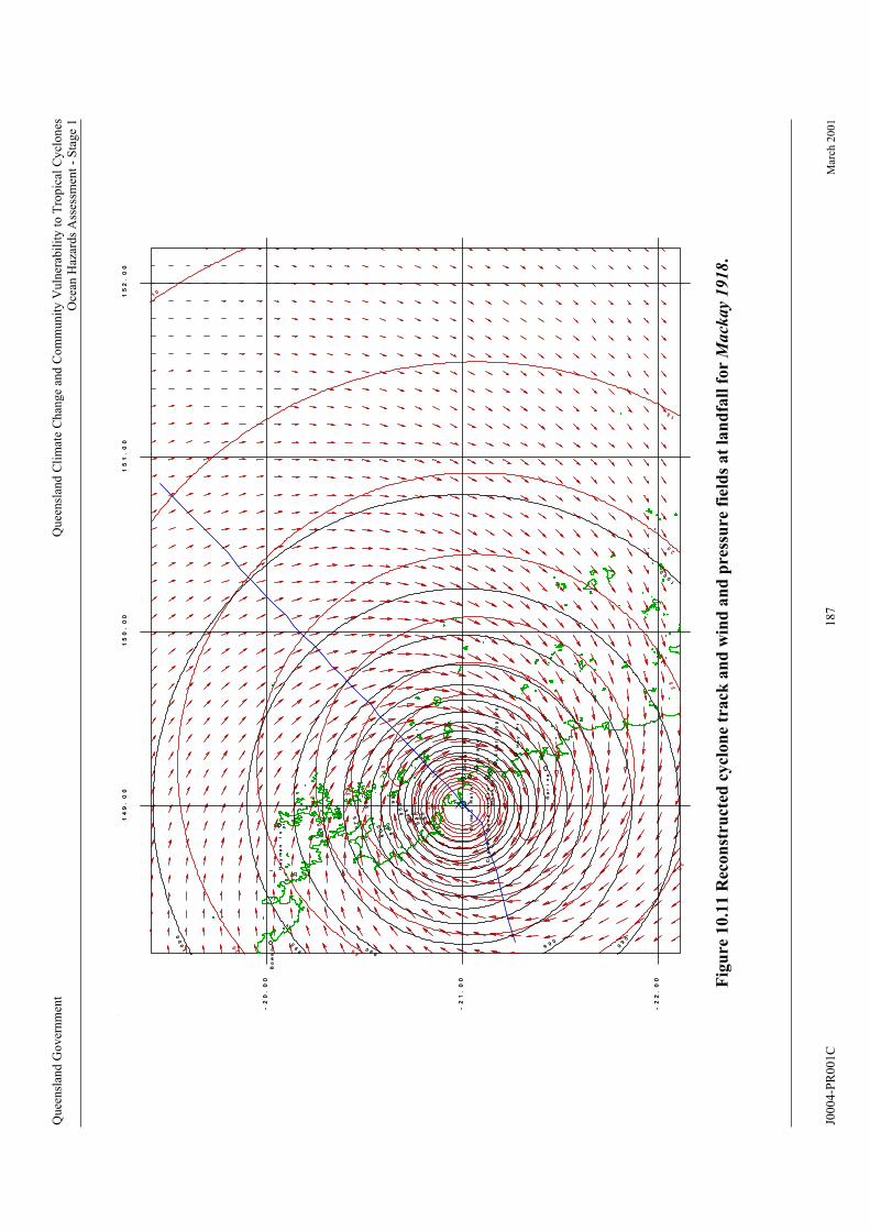
Quee
nsl
and G
over
nm
ent
Qu
een
slan
d C
lim
ate
Ch
ange
and
Co
mm
un
ity
Vuln
erab
ilit
y t
o T
rop
ical
Cy
clo
nes
Oce
an H
azar
ds
Ass
essm
ent
- S
tag
e 1
2
3
35
994
09
45
95
095
59
60
96
5
97
0
97
598
0
98
5
990 9
90
99
5
99
5
10
00
10
00
Bo
we
n
Sh
oa
l
Pt
Sl
ad
e
Pt
Ma
ck
ay
Ha
y
Pt
Sa
ri
na
Ha
ym
an
I
s
Fl
at
T
op
Is
J
Cr
ok
er
"B
on
aV
is
ta
"
Ei
me
o
Ho
te
l
-2
2.
00
-2
1.
00
-2
0.
00
14
9.
00
15
0.
00
15
1.
00
15
2.
00
2
3
35
994
09
45
95
095
59
60
96
5
97
0
97
598
0
98
5
990 9
90
99
5
99
5
10
00
10
00
Bo
we
n
Sh
oa
l
Pt
Sl
ad
e
Pt
Ma
ck
ay
Ha
y
Pt
Sa
ri
na
Ha
ym
an
I
s
Fl
at
T
op
Is
J
Cr
ok
er
"B
on
aV
is
ta
"
Ei
me
o
Ho
te
l
-2
2.
00
-2
1.
00
-2
0.
00
14
9.
00
15
0.
00
15
1.
00
15
2.
00
5
10
10
15
15
20
20
20
25
25
5
25
30
0
35
40
35
5
10
10
15
15
20
20
20
25
25
5
25
30
0
35
40
35
Fig
ure
10.1
1 R
econ
stru
cted
cycl
on
e tr
ack
an
d w
ind
an
d p
ress
ure
fie
lds
at
lan
dfa
ll f
or
Mack
ay
1918.
J0004-P
R001C
187
Mar
ch 2
00
1
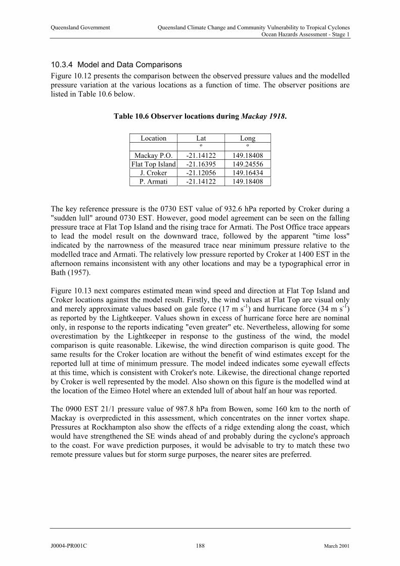
Queensland Government Queensland Climate Change and Community Vulnerability to Tropical CyclonesOcean Hazards Assessment - Stage 1
10.3.4 Model and Data Comparisons
Figure 10.12 presents the comparison between the observed pressure values and the modelledpressure variation at the various locations as a function of time. The observer positions are listed in Table 10.6 below.
Table 10.6 Observer locations during Mackay 1918.
Location Lat
Mackay P.O. -21.14122 149.18408
-21.16395
J. Croker -21.12056 149.16434
-21.14122 149.18408
Long
º º
Flat Top Island 149.24556
P. Armati
The key reference pressure is the 0730 EST value of 932.6 hPa reported by Croker during a "sudden lull" around 0730 EST. However, good model agreement can be seen on the falling pressure trace at Flat Top Island and the rising trace for Armati. The Post Office trace appearsto lead the model result on the downward trace, followed by the apparent "time loss" indicated by the narrowness of the measured trace near minimum pressure relative to the modelled trace and Armati. The relatively low pressure reported by Croker at 1400 EST in the afternoon remains inconsistent with any other locations and may be a typographical error in Bath (1957).
The 0900 EST 21/1 pressure value of 987.8 hPa from Bowen, some 160 km to the north of Mackay is overpredicted in this assessment, which concentrates on the inner vortex shape. Pressures at Rockhampton also show the effects of a ridge extending along the coast, which would have strengthened the SE winds ahead of and probably during the cyclone's approach to the coast. For wave prediction purposes, it would be advisable to try to match these two remote pressure values but for storm surge purposes, the nearer sites are preferred.
Figure 10.13 next compares estimated mean wind speed and direction at Flat Top Island and Croker locations against the model result. Firstly, the wind values at Flat Top are visual only and merely approximate values based on gale force (17 m s-1) and hurricane force (34 m s-1)as reported by the Lightkeeper. Values shown in excess of hurricane force here are nominalonly, in response to the reports indicating "even greater" etc. Nevertheless, allowing for someoverestimation by the Lightkeeper in response to the gustiness of the wind, the modelcomparison is quite reasonable. Likewise, the wind direction comparison is quite good. The same results for the Croker location are without the benefit of wind estimates except for the reported lull at time of minimum pressure. The model indeed indicates some eyewall effectsat this time, which is consistent with Croker's note. Likewise, the directional change reported by Croker is well represented by the model. Also shown on this figure is the modelled wind atthe location of the Eimeo Hotel where an extended lull of about half an hour was reported.
J0004-PR001C 188 March 2001

Quee
nsl
and G
over
nm
ent
Qu
een
slan
d C
lim
ate
Ch
ange
and
Co
mm
un
ity
Vuln
erab
ilit
y t
o T
rop
ical
Cy
clo
nes
Oce
an H
azar
ds
Ass
essm
ent
- S
tag
e 1
93
0
94
0
95
0
96
0
97
0
98
0
99
0
10
00
10
10
19
/01
/18
12
:00
20
/01
/18
00
:00
20
/01
/18
12
:00
21
/01
/18
00
:00
21
/01
/18
12
:00
22
/01
/18
00
:00
22
/01
/18
12
:00
MSL Pressure hPa
(a)
Mackay P
ost
Offi
ce
on f
lange
28"
Appare
nt tim
e lo
ss
93
0
94
0
95
0
96
0
97
0
98
0
99
0
10
00
10
10
19
/01
/18
12
:00
20
/01
/18
00
:00
20
/01
/18
12
:00
21
/01
/18
00
:00
21
/01
/18
12
:00
22
/01
/18
00
:00
22
/01
/18
12
:00
MSL Pressure hPa
Mo
de
lle
d
Me
as
ure
d
(c)
Priva
te O
bserv
er:
J.
Cro
ker "s
udden lu
ll"27.5
4"
Hg
(932.6
hPa)
93
0
94
0
95
0
96
0
97
0
98
0
99
0
10
00
10
10
19
/01
/18
12
:00
20
/01
/18
00
:00
20
/01
/18
12
:00
21
/01
/18
00
:00
21
/01
/18
12
:00
22
/01
/18
00
:00
22
/01
/18
12
:00
(d)
Priva
te O
bserv
er:
P.
Am
ati
on f
lange
28"
Hg
93
0
94
0
95
0
96
0
97
0
98
0
99
0
10
00
10
10
19
/01
/18
12
:00
20
/01
/18
00
:00
20
/01
/18
12
:00
21
/01
/18
00
:00
21
/01
/18
12
:00
22
/01
/18
00
:00
22
/01
/18
12
:00
(b)
Fla
t Top Isla
nd L
ightk
eeper
on f
lange
28"
Hg
J0004-P
R001C
189
Mar
ch 2
00
1
10
12
Fig
ure
. C
om
pari
son
of
mod
elle
d a
nd
mea
sure
d p
ress
ure
s fo
r M
ack
ay
1918.

Quee
nsl
and G
over
nm
ent
Qu
een
slan
d C
lim
ate
Ch
ange
and
Co
mm
un
ity
Vuln
erab
ilit
y t
o T
rop
ical
Cy
clo
nes
Oce
an H
azar
ds
Ass
essm
ent
- S
tag
e 1
0
20
40
60
80
10
0
12
0
14
0
16
0
18
0
19
/01
/18
12
:00
20
/01
/18
00
:00
20
/01
/18
12
:00
21
/01
/18
00
:00
21
/01
/18
12
:00
22
/01
/18
00
:00
22
/01
/18
12
:00
Wind Direction deg
Mo
de
lle
d
Ob
se
rve
d
(b)
Fla
tT
op
Isla
nd
Lig
htk
ee
pe
r-
Win
d D
ire
ctio
n
0
20
40
60
80
10
0
12
0
14
0
16
0
18
0
19
/01
/18
12
:00
20
/01
/18
00
:00
20
/01
/18
12
:00
21
/01
/18
00
:00
21
/01
/18
12
:00
22
/01
/18
00
:00
22
/01
/18
12
:00
Wind Direction deg
(d)
Priva
te O
bserv
er:
J. C
roker
- W
ind D
irections
05
10
15
20
25
30
35
40
45
50
19
/01
/18
12
:00
20
/01
/18
00
:00
20
/01
/18
12
:00
21
/01
/18
00
:00
21
/01
/18
12
:00
22
/01
/18
00
:00
22
/01
/18
12
:00
MeanWind Speedm/s
(a)
Fla
tT
op
Isla
nd
Lig
htk
ee
pe
r-
Win
d S
pe
ed
Es
tim
ate
s
05
10
15
20
25
30
35
40
45
50
19
/01
/18
12
:00
20
/01
/18
00
:00
20
/01
/18
12
:00
21
/01
/18
00
:00
21
/01
/18
12
:00
22
/01
/18
00
:00
22
/01
/18
12
:00
Mean WindSpeedm/s
(c)
Pri
vate
Ob
se
rve
r L
oca
tio
n:J. C
roke
r -
Win
dS
pe
ed
"su
dd
en
lu
ll"
at 0
7:3
0 ?
Eim
eo
Hote
l
Fig
ure
. C
om
pari
son
of
win
d s
pee
ds
an
d d
irec
tion
s fo
r M
ack
ay
1918
.10
13
J0004-P
R001C
190
Mar
ch 2
00
1
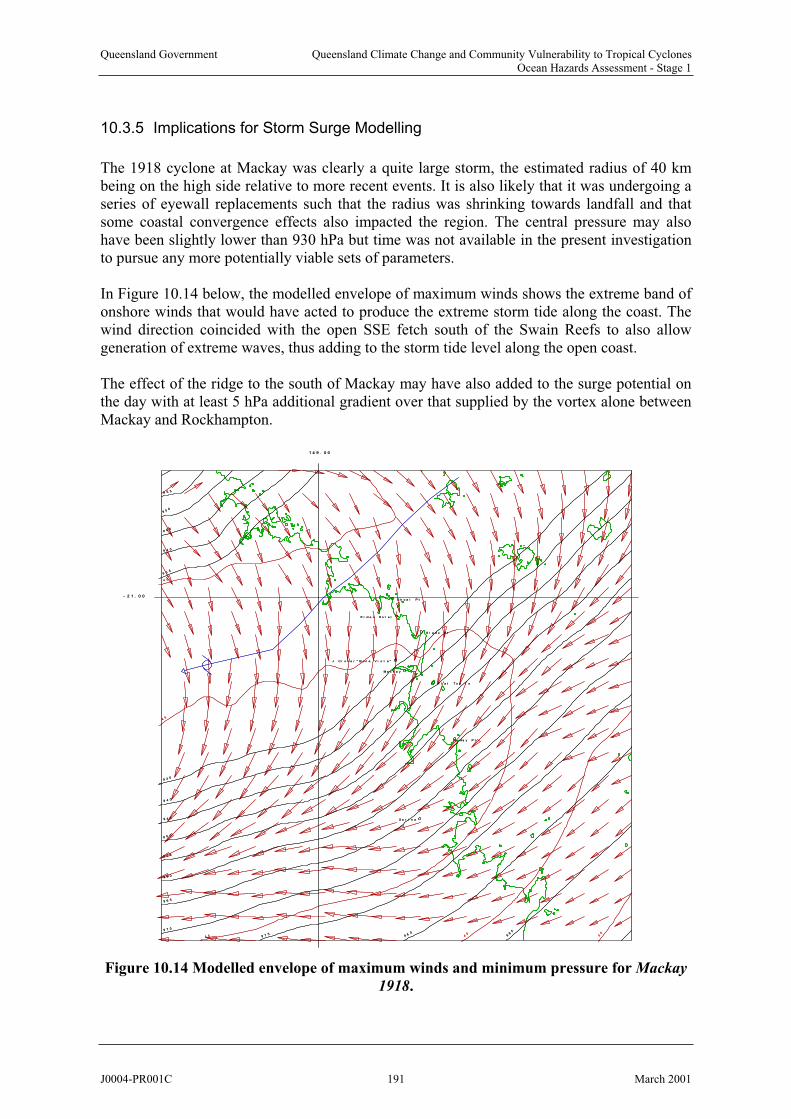
Queensland Government Queensland Climate Change and Community Vulnerability to Tropical CyclonesOcean Hazards Assessment - Stage 1
10.3.5 Implications for Storm Surge Modelling
The 1918 cyclone at Mackay was clearly a quite large storm, the estimated radius of 40 kmbeing on the high side relative to more recent events. It is also likely that it was undergoing a series of eyewall replacements such that the radius was shrinking towards landfall and that some coastal convergence effects also impacted the region. The central pressure may also have been slightly lower than 930 hPa but time was not available in the present investigationto pursue any more potentially viable sets of parameters.
In Figure 10.14 below, the modelled envelope of maximum winds shows the extreme band of onshore winds that would have acted to produce the extreme storm tide along the coast. The wind direction coincided with the open SSE fetch south of the Swain Reefs to also allow generation of extreme waves, thus adding to the storm tide level along the open coast.
The effect of the ridge to the south of Mackay may have also added to the surge potential on the day with at least 5 hPa additional gradient over that supplied by the vortex alone between Mackay and Rockhampton.
9 3 5
9 3 5
9 4 0
9 4 0
9 4 5
9 4 5
9 5 0
9 5 0
9 5 5
9 5 5
9 6 0
9 6 5
9 7 0
9 7 59 8
09
85
S h o a l P t
S l a d e P t
M a c k a y
H a y P t
S a r i n a
F l a t T o p I s
J C r o k e r " B o n a V i s t a "
E i m e o H o t e l
- 2 1 . 0 0
1 4 9 . 0 0
9 3 5
9 3 5
9 4 0
9 4 0
9 4 5
9 4 5
9 5 0
9 5 0
9 5 5
9 5 5
9 6 0
9 6 5
9 7 0
9 7 59 8
09
85
S h o a l P t
S l a d e P t
M a c k a y
H a y P t
S a r i n a
F l a t T o p I s
J C r o k e r " B o n a V i s t a "
E i m e o H o t e l
- 2 1 . 0 0
1 4 9 . 0 0
35
40
4 0
4 5
45
35
40
4 0
4 5
45
Figure 10.14 Modelled envelope of maximum winds and minimum pressure for Mackay
1918.
J0004-PR001C 191 March 2001

Queensland Government Queensland Climate Change and Community Vulnerability to Tropical CyclonesOcean Hazards Assessment - Stage 1
No wave modelling has been undertaken for the present investigation, but representative values are available from Harper (1983) - the spectral wave model study for the Half Tide Tug Harbour near Hay Point, south of Mackay. In that investigation a selection of modelcyclones was considered and two cases of landfall near Mackay are relevant: 925 hPa on a Wtrack and a 950 hPa on a SW track. Considering the 1918 event as a 930 hPa storm on a SW track, an indicative nearshore (< 5 km, 12 m depth) wave condition would be 7 m Hs with 8.5 s Tp. Applying Equation (8.19) then provides an order of magnitude estimate for shoreline setup of about 1 m at Far Beach.
Given that the peak water level reached at the town was 5.5 m AHD on a nominal 2 m AHDtide, and neglecting any other possible losses, the surge-only component could be as low as 2.5 m AHD at Far Beach, giving a SWL of about 4.5 m AHD. However, the extent to which wave setup in the river might have existed relative to Town Beach remains problematicalbecause the river mouth at the time was a mixture of natural sand bars and some training wallsdesigned to maintain a channel for navigation. It is also possible that there were overland flowlosses from the sea to the town centre, justifying perhaps a nominal reduction over that distance. Accordingly, a storm surge component closer to 3 m (yielding 5 m AHD SWL) might be indicated, to which wave setup of at least 0.5 m is to be added.
10.3.6 Tidal Modelling
As mentioned previously, extensive tidal modelling has previously been undertaken for this complex tidal region by James Cook University and 11 tidal constituents are used on the open boundaries. Figure 10.15 below shows the comparison between the predicted tide t2000) at Mackay Outer Harbour and the modelled tide. On the day of the storm tide the peak is particularly well matched, although the model tends to underpredict the low water levels. The modelled high tide of 2.01 m is 0.5 h ahead of the predicted maximum value of 1.98 m.
3 (Broadben
-2.0
-1.5
-1.0
-0.5
0.0
0.5
1.0
1.5
2.0
20
12:00
20
15:00
20
18:00
20
21:00
21
00:00
21
03:00
21
06:00
21
09:00
21
12:00
Time UTC
Wate
r L
evel
(m A
HD
)
Predicted Tide
Modelled Tide
Figure 10.15 Comparison of modelled and predicted tide during Mackay 1918.
3 It is also possible that the supplied predicted tide is subject to some error (J. Broadbent, pers comm)
J0004-PR001C 192 March 2001
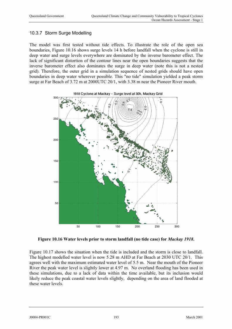
Queensland Government Queensland Climate Change and Community Vulnerability to Tropical CyclonesOcean Hazards Assessment - Stage 1
10.3.7 Storm Surge Modelling
The model was first tested without tide effects. To illustrate the role of the open sea boundaries, Figure 10.16 shows surge levels 14 h before landfall when the cyclone is still in deep water and surge levels everywhere are dominated by the inverse barometer effect. The lack of significant distortion of the contour lines near the open boundaries suggests that the inverse barometer effect also dominates the surge in deep water (note this is not a nestedgrid). Therefore, the outer grid in a simulation sequence of nested grids should have open boundaries in deep water wherever possible. This "no tide" simulation yielded a peak storm surge at Far Beach of 3.72 m at 2000UTC 20/1, with 3.38 m near the Pioneer River mouth.
0 16Figure 1 . Water levels prior to storm landfall (no tide case) for Mackay 1918.
Figure 10.17 shows the situation when the tide is included and the storm is close to landfall. The highest modelled water level is now 5.28 m AHD at Far Beach at 2030 UTC 20/1. This agrees well with the maximum estimated water level of 5.5 m. Near the mouth of the Pioneer River the peak water level is slightly lower at 4.97 m. No overland flooding has been used in these simulations, due to a lack of data within the time available, but its inclusion would likely reduce the peak coastal water levels slightly, depending on the area of land flooded at these water levels.
J0004-PR001C 193 March 2001

Queensland Government Queensland Climate Change and Community Vulnerability to Tropical CyclonesOcean Hazards Assessment - Stage 1
Mackay
Mackay
Figure 10.17 Storm tide elevations and velocities at landfall (tide included) for Mackay
1918.
J0004-PR001C 194 March 2001

Queensland Government Queensland Climate Change and Community Vulnerability to Tropical CyclonesOcean Hazards Assessment - Stage 1
The maximum storm surge in this case (i.e. total water level - tide) at Far Beach is 3.29 m,0.43 m below the surge without the tide (a 12% reduction) due to the nonlinear interaction of the surge and tide. Because the tide level was rising as the storm approached the coast, the surface wind stress effect was slightly less in the deepening coastal waters. If the cyclone had arrived at low tide, the surge component may have increased but the total storm tide level would have been much reduced.
The results of the simulations are summarised in Figure 10.18, comparing the modelled levels with the estimated value of inundation in the town and the reported timing of the onset of flooding (i.e. levels above HAT). Considering the poor storm data available, the agreement isvery satisfactory and is consistent with a potential wave setup component of at least 0.5 mneeded to reach the 5.5 m AHD town level. Also of interest is the model prediction that waterlevels to the south are slightly higher than to the north, supporting the eyewitness accounts that the surge first entered the town from the south-east and then flowed northwards towards the river.
A further model test was then undertaken to determine the effect of the Great Barrier Reef on the predicted storm tide levels at Mackay and the results are summarised in Figure 10.19.Firstly, the difference between the surge magnitudes alone, with and without the reef present, show a small reduction of only 0.1 m (this adds the modelled surge at MSL to the predictedtide). Hence, the surge is mainly generated inside the reef on the relatively broad continentalshelf that extends to the south east. However, if the tide is also modelled but without the reef
-2
-1
0
1
2
3
4
5
6
20
14:00
20
15:00
20
16:00
20
17:00
20
18:00
20
19:00
20
20:00
20
21:00
20
22:00
20
23:00
21
00:00
21
01:00
Time UTC
Wate
r L
evel
m A
HD
Tide
Measured
JCU Pioneer R
JCU Far BeachHAT
crosses coast
21:30 UTC
Peak Level 5.5m
Figure 10.18 Time history comparisons of modelled and measured water levels for the
Mackay 1918 cyclone.
J0004-PR001C 195 March 2001
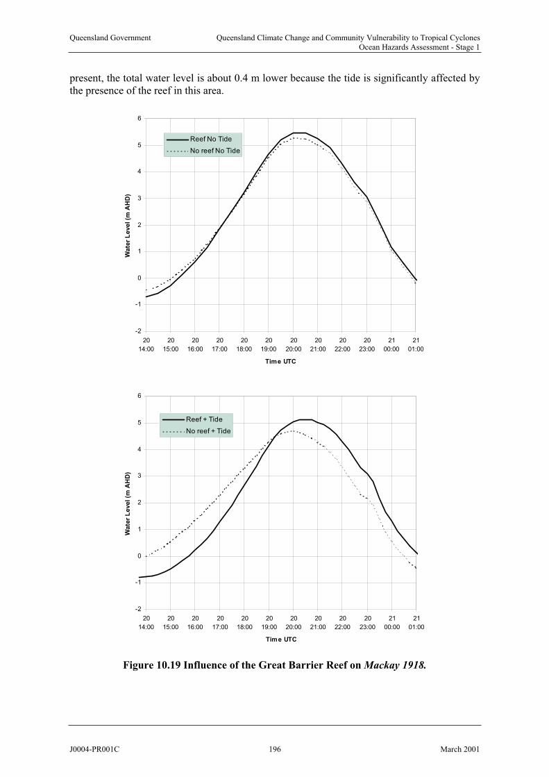
Queensland Government Queensland Climate Change and Community Vulnerability to Tropical CyclonesOcean Hazards Assessment - Stage 1
present, the total water level is about 0.4 m lower because the tide is significantly affected by the presence of the reef in this area.
0 9
-2
-1
0
1
2
3
4
5
6
20
14:00
20
15:00
20
16:00
20
17:00
20
18:00
20
19:00
20
20:00
20
21:00
20
22:00
20
23:00
21
00:00
21
01:00
Time UTC
Wate
r L
evel (m
AH
D)
Reef No Tide
No reef No Tide
-2
-1
0
1
2
3
4
5
6
20
14:00
20
15:00
20
16:00
20
17:00
20
18:00
20
19:00
20
20:00
20
21:00
20
22:00
20
23:00
21
00:00
21
01:00
Time UTC
Wate
r L
evel (m
AH
D)
Reef + Tide
No reef + Tide
Figure 1 .1 Influence of the Great Barrier Reef on Mackay 1918.
J0004-PR001C 196 March 2001

Queensland Government Queensland Climate Change and Community Vulnerability to Tropical CyclonesOcean Hazards Assessment - Stage 1
10.3.8 References
AGSO (2000) Community risk in Mackay - a multi-hazard risk assessment. Australian
Geological Survey Organisation, Cities Project, ISBN 0 642 398623 (CD-ROM).
Broadbent G.J. (2000) Personal communication. Queensland Department of Transport.
Callaghan J. (2000) Personal communication. Bureau of Meteorology, Queensland RegionalOffice.
Croker P. (2000) Personal communication. Letter by Phyllis MacArthur, March 1st 1918.
Davidson, J.T., Hubbert, G.D., Woodcock, F., Bergin, M. and Morison, R. (1993) Modelling storm surge in the Mackay Region. Proc 11th Aust Conf Coastal and Ocean Engin. IEAust.Aug.
Bath A.T. (1957) The Mackay cyclone of 21 January, 1918. Aust Met Mag, 19, Dec 1957, 46-59.
Gourlay M.R. and Hacker J.L.F. (1986) Pioneer River estuary sedimentation studies. Dept of Civil Engin, The University of Queensland.
Gourlay M.R. (2000) Personal communication. The University of Queensland.
Harbours and Rivers Department (1918) Report from the engineer for harbours and rivers for the year ended 30th June, 1918. Govt of Queensland, C.A.58-1918.
Harper B.A. (1983) Half Tide tug harbour - tropical cyclone spectral wave modelling study.
Report prepared by Blain Bremner and Williams Pty Ltd for the DBCT-UDC Joint Venture, Sep.
Harper B.A. and Holland G.J. (1999) An updated parametric model of the tropical cyclone. Proc. 23rd Conf. Hurricanes and Tropical Meteorology, AMS, Dallas, Texas, 10-15 Jan.
Lourensz, R.S. (1981) Tropical cyclones in the Australian Region July 1909 to June 1980. Bureau of Meteorology. Oct.
Daily Mercury (1918) Monday January 28th 1918.
Daily Mercury (1993) 1918 The big blow. Special Feature. Wednesday January 27th 1993.
Parkinson C.E., Fison E.C., Leach R.A. and Wilmoth G.R. (1950) Flooding in the Pioneer River and its effect on the Mackay City area. Report of Committee of Enquiry to the Co-
ordinator General of Public Works, Brisbane.
Visher S.S. and Hodge D. (1925) Australian hurricanes and related storms. Bureau of
Meteorology, Feb, 54pp
J0004-PR001C 197 March 2001
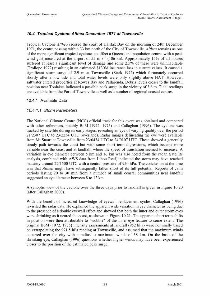
Queensland Government Queensland Climate Change and Community Vulnerability to Tropical CyclonesOcean Hazards Assessment - Stage 1
10.4 Tropical Cyclone Althea December 1971 at Townsville
Tropical Cyclone Althea crossed the coast of Halifax Bay on the morning of 24th December1971, the centre passing within 33 km north of the City of Townsville. Althea remains as oneof the more significant tropical cyclones to affect a Queensland population centre, with a peak wind gust measured at the airport of 55 m s ately 15% of all houses suffered at least a significant level of damage and some 2.5% of these were uninhabitable (Trollope 1972) resulting in an estimated $130M insurance loss in current values. It caused a significant storm surge of 2.9 m at Townsville (Stark 1972) which fortunately occurredshortly after a low tide and total water levels were only slightly above HAT. However, saltwater entered properties at Rowes Bay and Pallarenda. Debris levels closer to the landfallposition near Toolakea indicated a possible peak surge in the vicinity of 3.6 m. Tidal readingsare available from the Port of Townsville as well as a number of regional coastal centres.
10.4.1 Available Data
-1 (106 kn). Approxim
10.4.1.1 Storm Parameters
The National Climate Centre (NCC) official track for this event was obtained and comparedwith other references, notably BoM (1972, 1975) and Callaghan (1996). The cyclone wastracked by satellite during its early stages, revealing an eye of varying quality over the period21/2307 UTC to 23/2254 UTC (overland). Radar images delineating the eye were available from Mt Stuart at Townsville from 23/0434 UTC to 24/0107 UTC. These showed a generally steady path towards the coast but with some short term digressions, which became morevariable near the coast and at landfall, where the speed of translation seemed to increase. Avariation in eye diameter between 5 km and 16 km was also noted from the radar. Satelliteanalysis, combined with AWS data from Lihou Reef, indicated the storm may have reachedmaturity around 22/1500 UTC with a central pressure of 950 hPa. The conclusion at the timewas that Althea might have subsequently fallen short of its full potential. Reports of calmperiods lasting 20 to 30 min from a number of small coastal communities near landfallsuggested an eye diameter between 8 to 12 km.
A synoptic view of the cyclone over the three days prior to landfall is given in Figure 10.20 (after Callaghan 2000).
With the benefit of increased knowledge of eyewall replacement cycles, Callaghan (1996) revisited the radar data. He explained the apparent wide variation in eye diameter as being dueto the presence of a double eyewall effect and showed that both the inner and outer storm eyeswere shrinking as it neared the coast, as shown in Figure 10.21. The apparent short term shiftsin position were then attributable to "wobble" of the inner eye feature to some extent. The original BoM (1972, 1975) intensity assessments at landfall (952 hPa) were nominally based on extrapolating the 971.5 hPa reading at Townsville, and assumed that the maximum winds occurred over the city with a radius to maximum winds of 38 km. On the basis of the shrinking eye, Callaghan (1996) questions whether higher winds may have been experienced closer to the position of the estimated peak surge.
J0004-PR001C 198 March 2001
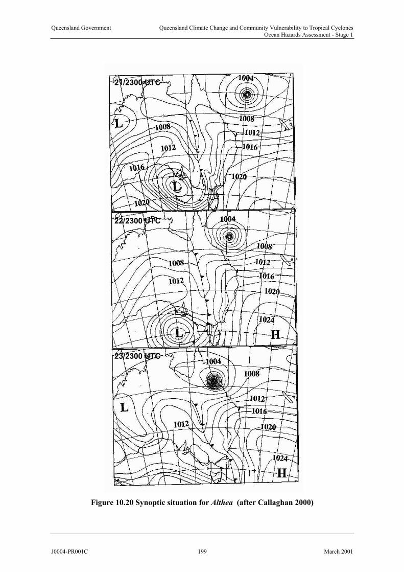
Queensland Government Queensland Climate Change and Community Vulnerability to Tropical CyclonesOcean Hazards Assessment - Stage 1
21/2300 UTC21/2300 UTC
22/2300 UTC22/2300 UTC
23/2300 UTC23/2300 UTC
Figure 10.20 Synoptic situation for Althea (after Callaghan 2000)
J0004-PR001C 199 March 2001

Queensland Government Queensland Climate Change and Community Vulnerability to Tropical CyclonesOcean Hazards Assessment - Stage 1
23/2108 UTC
23/2209 UTC
23/2302 UTC
RADAR
AMOTOOLAKEA
Figure 10.21 Radar images of Althea (after Callaghan 1996).
The barograph and Dines anemograph records from Townsville Airport are reproduced inFigure 10.22, taken from BoM (1972).
J0004-PR001C 200 March 2001
Queensland Government Queensland Climate Change and Community Vulnerability to Tropical CyclonesOcean Hazards Assessment - Stage 1
Figure 10.22 Barograph (top) and anemograph (bottom) from Townsville Airport.
J0004-PR001C 201 March 2001

Queensland Government Queensland Climate Change and Community Vulnerability to Tropical CyclonesOcean Hazards Assessment - Stage 1
10.4.1.2 Storm Surge
The impact of the Althea storm surge extended over an extensive period of coastline, being at least 0.5 m above predicted tide between Cairns, 290 km to the north and Mackay, 320 km to the south. Chart recording tide gauges at a number of sites provided accurate water level values and these were able to be augmented with estimates from a beach debris surveyundertaken between Ingham and Ayr (Stark 1972).
BoM (1975) also reports some debris estimates from a Townsville Harbour Board report by E.M. Shepherd which clearly includes wave setup and runup influences. Table 10.7 below summarises these values, with positive landfall distances indicating southwards of the track.The Tobruk Pool reading* is reputedly "stillwater" inside the kiosk, presumably represented by a watermark. If accurate, this represents a possible 2 m wave setup and runup componentat this point, which is quite close to the harbour tide gauge. At North Ward, Shepherd reported another debris level estimate of 5.84 m AHD as the limit of storm tide influence.
Table 10.7 Summary of estimated peak storm surge amplitude for Althea.
LocationDistance
fromLandfall
LevelReference
SurgeAmplitude
km m
Cairns -240 gauge 0.5
0.8
Lucinda -50 gauge 0.9
Balgal -18 debris 1.8 ?
Toolakea 19 debris > 3.6 ?
26 debris > 3.1 ?
Black River 30 debris 2.7 - 3.1 ?
Tobruk Pool 46.5 mark* 4.9*
Townsville 47 gauge 2.9
Cungulla 88 debris 2.1 ?
Alva Beach 132 debris 1.8 ?
147 debris < 1.8
Bowen 227 gauge 1.0
385 gauge 0.9
Mourilyan -155 gauge
Saunders Beach
Beach Mount Beach
Mackay
J0004-PR001C 202 March 2001

Queensland Government Queensland Climate Change and Community Vulnerability to Tropical CyclonesOcean Hazards Assessment - Stage 1
0.0
0.5
1.0
1.5
2.0
2.5
3.0
3.5
4.0
-300 -200 -100 0 100 200 300 400
Distance from Landfall km
Su
rge A
mp
litu
de
m
Figure 10.23 Alongshore variation in estimated peak storm surge amplitude for Althea.
The following describes the result of a trial and error comparison between the available dataand the predicted spatial and temporal variations in wind and pressure as predicted by an analytical model (Harper and Holland 1999), detailed in Appendix C. The model was systematically adjusted for reasonable values of the key parameters such as track, central pressure, windfield peakedness and radius to maximum winds. The available data from Townsville and a number AWS locations were then compared with the model output to determine the validity of the various assumptions. This was initially done objectively without reference to the effect of the reconstructed windfield on the generated storm surge. However, subsequent storm surge modelling identified a significant sensitivity to the assumed windfield
asymmetry, namely lly chosen as 65 based on currently acceptedtheory (refer Chapter 5). The final windfield calibration has adopted a "left rear" wind
maxima of 115 and differences from the 65 assumption (left front) are indicated. The "left rear" assumption not only significantly improves the wind speed calibration at the majority of sites but also the storm surge result. Whilst this change might be due to a better representation of the outer windfield asymmetry it also significantly improves the wind speed comparisonwith sites closer to the storm centre.
Only the Townsville Harbour gauge can be considered a reliable "stillwater" surge amplitude because of its location within the harbour at the entrance to Ross Creek. The tide stilling basin filters the effects of any waves present and wave setup is not expected to occur inside theharbour due to its diffractive qualities, e.g. Dunn et al. (2000). The remaining values derived from debris heights remain indicative only for purposes of comparison with a modelprediction because of the difficulty in not only estimating local RLs but also the influence of wave setup and runup on debris lines. All these levels are summarised on Figure 10.23.
Figures 10.24 and 10.25 show the tide gauge records from Townsville and Bowen,overplotted with the predicted tide and the resulting surge amplitude component. The stormtide at the Townsville gauge peaked at 2.53 m AHD, with a surge magnitude of 2.9 m.
10.4.2 Reconstruction of the Event
max, which was origina
J0004-PR001C 203 March 2001

Queensland Government Queensland Climate Change and Community Vulnerability to Tropical CyclonesOcean Hazards Assessment - Stage 1
-1.0
-0.5
0.0
0.5
1.0
1.5
2.0
2.5
3.0
3.5
23/12/71 00:00 23/12/71 12:00 24/12/71 00:00 24/12/71 12:00 25/12/71 00:00
UTC
Wa
ter
Le
ve
l m
Predicted Tide
Recorded
SurgeHAT 2.15 m AHD
Figure 1 .2 Tidal record at Townsville harbour during Althea.0 4
-1.0
-0.5
0.0
0.5
1.0
1.5
2.0
2.5
3.0
3.5
23/12/71 00:00 23/12/71 12:00 24/12/71 00:00 24/12/71 12:00 25/12/71 00:00
UTC
Wa
ter
Le
ve
l m
Predicted Tide
Recorded
SurgeHAT 1.95 m AHD
Figure 10.25 Tidal record at Bowen harbour during Althea.
J0004-PR001C 204 March 2001
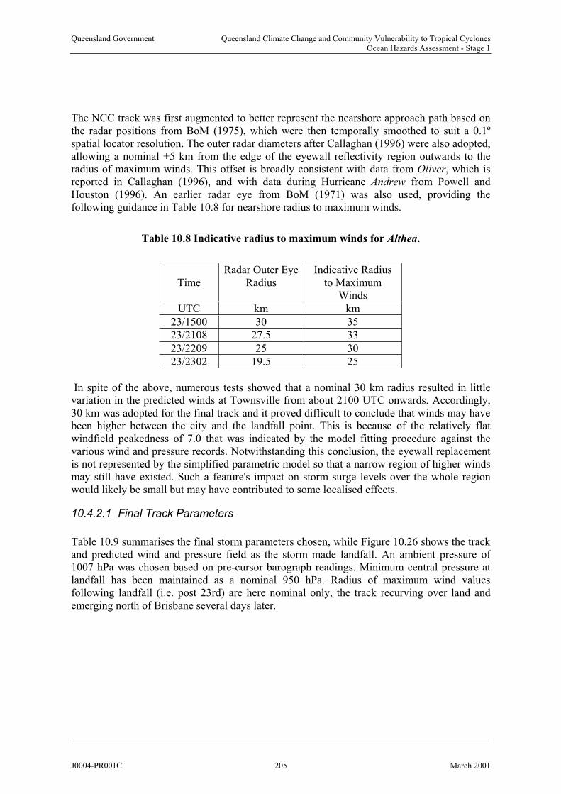
Queensland Government Queensland Climate Change and Community Vulnerability to Tropical CyclonesOcean Hazards Assessment - Stage 1
The NCC track was first augmented to better represent the nearshore approach path based on the radar positions from BoM (1975), which were then temporally smoothed to suit a 0.1ºspatial locator resolution. The outer radar diameters after Callaghan (1996) were also adopted, allowing a nominal +5 km from the edge of the eyewall reflectivity region outwards to the radius of maximum winds. This offset is broadly consistent with data from Oliver, which is reported in Callaghan (1996), and with data during Hurricane Andrew from Powell and Houston (1996). An earlier radar eye from BoM (1971) was also used, providing the following guidance in Table 10.8 for nearshore radius to maximum winds.
Table 10.8 Indicative radius to maximum winds for Althea.
TimeRadar Outer Eye
RadiusIndicative Radius
to MaximumWinds
UTC km km
23/1500 30 35
23/2108 27.5 33
30
23/2302 19.5 25
23/2209 25
In spite of the above, numerous tests showed that a nominal 30 km radius resulted in little variation in the predicted winds at Townsville from about 2100 UTC onwards. Accordingly,30 km was adopted for the final track and it proved difficult to conclude that winds may havebeen higher between the city and the landfall point. This is because of the relatively flat windfield peakedness of 7.0 that was indicated by the model fitting procedure against the various wind and pressure records. Notwithstanding this conclusion, the eyewall replacementis not represented by the simplified parametric model so that a narrow region of higher windsmay still have existed. Such a feature's impact on storm surge levels over the whole regionwould likely be small but may have contributed to some localised effects.
10.4.2.1 Final Track Parameters
Table 10.9 summarises the final storm parameters chosen, while Figure 10.26 shows the track and predicted wind and pressure field as the storm made landfall. An ambient pressure of 1007 hPa was chosen based on pre-cursor barograph readings. Minimum central pressure at landfall has been maintained as a nominal 950 hPa. Radius of maximum wind valuesfollowing landfall (i.e. post 23rd) are here nominal only, the track recurving over land andemerging north of Brisbane several days later.
J0004-PR001C 205 March 2001
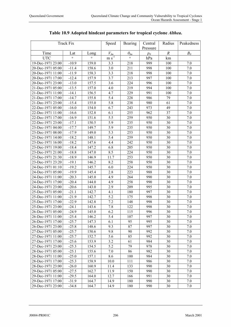
Queensland Government Queensland Climate Change and Community Vulnerability to Tropical CyclonesOcean Hazards Assessment - Stage 1
Table 10.9 Adopted hindcast parameters for tropical cyclone Althea.
Track Fix Speed Bearing CentralPressure
Radius Peakedness
Time Lat Long Vfm fm p0 R B0
m s-1 hPa km
19-Dec-1971 23:00 -10.9 159.0 3.3 218 999 100 7.0
20-Dec-1971 05:00 -11.4 158.6 3.0 211 998 100 7.0
20-Dec-1971 11:00 -11.9 158.3 3.3 218 998 100 7.0
-12.4 157.9 3.7 213 997 100 7.0
20-Dec-1971 23:00 -13.0 157.5 3.6 224 996 100 7.0
21-Dec-1971 05:00 -13.5 157.0 4.0 219 994 100 7.0
-14.1 156.5 4.7 229 100 7.0
21-Dec-1971 17:00 -14.7 155.8 5.4 228 7.0986 79
21-Dec-1971 23:00 -15.4 155.0 5.8 238 980 61 7.0
22-Dec-1971 05:00 -16.0 154.0 6.7 243 973 49 7.0
22-Dec-1971 11:00 -16.6 152.8 6.1 255 962 37 7.0
22-Dec-1971 17:00 -16.9 151.6 5.5 259 950 30 7.0
22-Dec-1971 23:00 -17.1 150.5 5.9 235 950 30 7.0
23-Dec-1971 04:00 -17.7 149.7 5.9 235 950 30 7.0
-17.9 149.0 5.3 253 950 30 7.0
23-Dec-1971 14:00 -18.2 148.1 5.4 259 950 30 7.0
23-Dec-1971 16:00 -18.2 147.6 4.4 242 950 30 7.0
23-Dec-1971 19:00 -18.4 147.2 6.8 205 950 30 7.0
23-Dec-1971 21:00 -18.8 147.0 8.5 224 950 30 7.0
23-Dec-1971 21:30 -18.9 146.9 11.7 253 950 30 7.0
23-Dec-1971 23:20 -19.1 146.2 8.2 258 950 30 7.0
24-Dec-1971 01:10 -19.2 145.7 6.0 224 950 30 7.0
24-Dec-1971 05:00 -19.9 145.4 2.8 223 988 30 7.0
24-Dec-1971 11:00 -20.3 145.0 4.9 264 990 30 7.0
24-Dec-1971 17:00 -20.4 144.0 4.9 258 990 30 7.0
24-Dec-1971 23:00 -20.6 143.0 2.9 209 995 30 7.0
25-Dec-1971 05:00 -21.1 142.7 4.1 180 997 30 7.0
25-Dec-1971 11:00 -21.9 142.7 5.2 175 998 30 7.0
25-Dec-1971 17:00 -22.9 142.8 7.2 148 998 30 7.0
25-Dec-1971 23:00 -24.1 143.6 7.8 122 998 30 7.0
26-Dec-1971 05:00 -24.9 145.0 6.2 115 996 30 7.0
26-Dec-1971 11:00 -25.4 146.2 5.4 107 997 30
-25.7 147.3 6.1 95 995 30 7.0
26-Dec-1971 23:00 -25.8 148.6 9.3 87 997 30 7.0
-25.7 150.6 9.8 90 992 30 7.0
27-Dec-1971 11:00 -25.7 152.7 5.6 85 992 30 7.0
27-Dec-1971 17:00 -25.6 153.9 3.2 61 984 30 7.0
27-Dec-1971 23:00 -25.3 154.5 5.2 79 978 30 7.0
-25.1 155.6 7.0 86 982 30 7.0
28-Dec-1971 11:00 -25.0 157.1 8.6 100 984 30 7.0
28-Dec-1971 17:00 -25.3 158.9 10.0 111 986 30 7.0
28-Dec-1971 23:00 -26.0 160.9 11.4 133 990 30 7.0
29-Dec-1971 05:00 -27.5 162.7 11.9 150 990 30 7.0
29-Dec-1971 11:00 -29.5 164.0 12.7 166 991 30 7.0
29-Dec-1971 17:00 -31.9 164.7 14.9 180 990 30 7.0
29-Dec-1971 23:00 -34.8 164.7 14.9 180 990 30 7.0
UTC
20-Dec-1971 17:00
21-Dec-1971 11:00 991
23-Dec-1971 08:00
7.0
26-Dec-1971 17:00
27-Dec-1971 05:00
28-Dec-1971 05:00
J0004-PR001C 206 March 2001

Quee
nsl
and G
over
nm
ent
Qu
een
slan
d C
lim
ate
Ch
ange
and
Co
mm
un
ity
Vuln
erab
ilit
y t
o T
rop
ical
Cy
clo
nes
Oce
an H
azar
ds
Ass
essm
ent
- S
tag
e 1
1
95
5
96
0
96
5
97
0
97
5
98
0
98
5
99
0
99
5
99
5
10
00
Ca
rd
we
ll
To
wn
sv
il
le
Bo
we
n
In
ni
sf
ai
l
Ca
rd
we
ll
Ha
ym
an
I
s
Fl
in
de
rs
R
ee
f
In
gh
am
-2
0.
00
-1
9.
00
-1
8.
00
14
6.
00
14
7.
00
14
8.
00
14
9.
00
1
95
5
96
0
96
5
97
0
97
5
98
0
98
5
99
0
99
5
99
5
10
00
Ca
rd
we
ll
To
wn
sv
il
le
Bo
we
n
In
ni
sf
ai
l
Ca
rd
we
ll
Ha
ym
an
I
s
Fl
in
de
rs
R
ee
f
In
gh
am
-2
0.
00
-1
9.
00
-1
8.
00
14
6.
00
14
7.
00
14
8.
00
14
9.
00
5
10
5
15
15
20
20
25
25
30
35
40
5
10
5
15
15
20
20
25
25
30
35
40
Fig
ure
. R
econ
stru
cted
cycl
on
e tr
ack
an
d w
ind
an
d p
ress
ure
fie
lds
nea
r la
nd
fall
for
Alt
hea
.10
26
J0004-P
R001C
207
Mar
ch 2
00
1
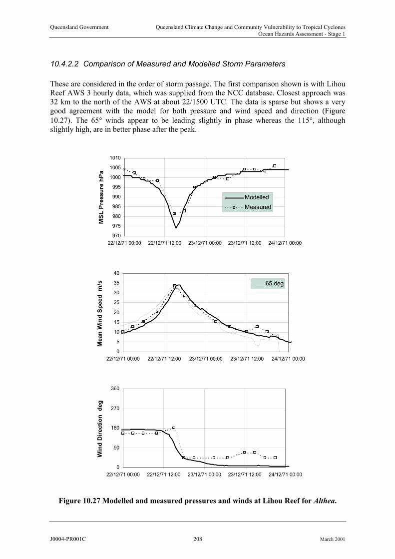
Queensland Government Queensland Climate Change and Community Vulnerability to Tropical CyclonesOcean Hazards Assessment - Stage 1
10.4.2.2 Comparison of Measured and Modelled Storm Parameters
These are considered in the order of storm passage. The first comparison shown is with Lihou Reef AWS 3 hourly data, which was supplied from the NCC database. Closest approach was 32 km to the north of the AWS at about 22/1500 UTC. The data is sparse but shows a very good agreement with the model for both pressure and wind speed and direction (Figure
10.27). The 65 winds appear to be leading slightly in phase whereas the 115 , although slightly high, are in better phase after the peak.
970
975
980
985
990
995
1000
1005
1010
22/12/71 00:00 22/12/71 12:00 23/12/71 00:00 23/12/71 12:00 24/12/71 00:00
MS
L P
ressu
reh
Pa
Modelled
Measured
0
5
10
15
20
25
30
35
40
22/12/71 00:00 22/12/71 12:00 23/12/71 00:00 23/12/71 12:00 24/12/71 00:00
Mean
Win
dS
peed
m/s 65 deg
0
90
180
270
360
22/12/71 00:00 22/12/71 12:00 23/12/71 00:00 23/12/71 12:00 24/12/71 00:00
Win
d D
irecti
on
deg
Figure 10.27 Modelled and measured pressures and winds at Lihou Reef for Althea.
J0004-PR001C 208 March 2001

Queensland Government Queensland Climate Change and Community Vulnerability to Tropical CyclonesOcean Hazards Assessment - Stage 1
Figure 10.28 shows the comparison with Willis Island AWS, where closest storm approach
was about 102 km to the SSE near 23/0000. The model pressure and the 65 winds are leading
the measured values by about 5 to 6 hours, whereas the adopted 115 winds are slightly leading also but again match the post-peak measured winds more accurately.
992
994
996
998
1000
1002
1004
1006
1008
1010
22/12/71 00:00 22/12/71 12:00 23/12/71 00:00 23/12/71 12:00 24/12/71 00:00
MS
L P
ressu
re h
Pa
Modelled
Measured
0
2
4
6
8
10
12
14
16
18
20
22/12/71 00:00 22/12/71 12:00 23/12/71 00:00 23/12/71 12:00 24/12/71 00:00
Mean
Win
d S
peed
m
/s 65 deg
0
90
180
270
360
22/12/71 00:00 22/12/71 12:00 23/12/71 00:00 23/12/71 12:00 24/12/71 00:00
Win
d D
irecti
on
deg
Figure 10.28 Modelled and measured pressures and winds at Willis Island for Althea.
Figure 10.29 shows the comparison with Flinders Reef AWS, where closest approach of 35km to the SSE occurred near 23/1100 UTC, placing the site close to the eyewall. Again, the
comparisons are very good although there is a hint of the eye in the data. While the 115model does not perform as well as the 65º prior to the peak it is again better after the peak.
J0004-PR001C 209 March 2001
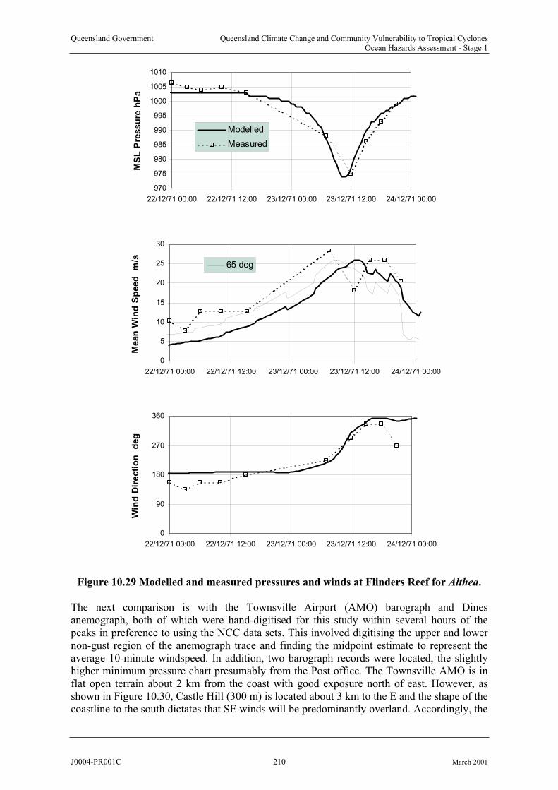
Queensland Government Queensland Climate Change and Community Vulnerability to Tropical CyclonesOcean Hazards Assessment - Stage 1
970
975
980
985
990
995
1000
1005
1010
22/12/71 00:00 22/12/71 12:00 23/12/71 00:00 23/12/71 12:00 24/12/71 00:00
MS
L P
ressu
re h
Pa
Modelled
Measured
0
5
10
15
20
25
30
22/12/71 00:00 22/12/71 12:00 23/12/71 00:00 23/12/71 12:00 24/12/71 00:00
Mean
Win
d S
peed
m
/s
65 deg
0
90
180
270
360
22/12/71 00:00 22/12/71 12:00 23/12/71 00:00 23/12/71 12:00 24/12/71 00:00
Win
d D
irecti
on
d
eg
Figure 10.29 Modelled and measured pressures and winds at Flinders Reef for Althea.
The next comparison is with the Townsville Airport (AMO) barograph and Dines anemograph, both of which were hand-digitised for this study within several hours of the peaks in preference to using the NCC data sets. This involved digitising the upper and lower non-gust region of the anemograph trace and finding the midpoint estimate to represent theaverage 10-minute windspeed. In addition, two barograph records were located, the slightlyhigher minimum pressure chart presumably from the Post office. The Townsville AMO is in flat open terrain about 2 km from the coast with good exposure north of east. However, as shown in Figure 10.30, Castle Hill (300 m) is located about 3 km to the E and the shape of thecoastline to the south dictates that SE winds will be predominantly overland. Accordingly, the
J0004-PR001C 210 March 2001
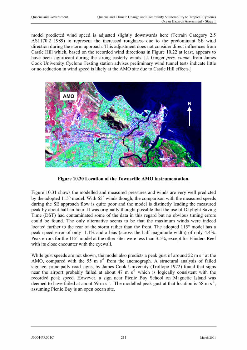
Queensland Government Queensland Climate Change and Community Vulnerability to Tropical CyclonesOcean Hazards Assessment - Stage 1
model predicted wind speed is adjusted slightly downwards here (Terrain Category 2.5 AS1170.2 1989) to represent the increased roughness due to the predominant SE wind direction during the storm approach. This adjustment does not consider direct influences from Castle Hill which, based on the recorded wind directions in Figure 10.22 at least, appears to have been significant during the strong easterly winds. [J. Ginger pers. comm. from JamesCook University Cyclone Testing station advises preliminary wind tunnel tests indicate little or no reduction in wind speed is likely at the AMO site due to Castle Hill effects.]
AMO
N
Figure 1 .3 Location of the Townsville AMO instrumentation.0 0
Figure 10.31 shows the modelled and measured pressures and winds are very well predicted
by the adopted 115 model. With 65 winds though, the comparison with the measured speeds during the SE approach flow is quite poor and the model is distinctly leading the measuredpeak by about half an hour. It was originally thought possible that the use of Daylight Saving Time (DST) had contaminated some of the data in this regard but no obvious timing errors could be found. The only alternative seems to be that the maximum winds were indeed
located further to the rear of the storm rather than the front. The adopted 115 model has a peak speed error of only -1.1% and a bias (across the half-magnitude width) of only 4.4%.
Peak errors for the 115 model at the other sites were less than 3.5%, except for Flinders Reef with its close encounter with the eyewall.
While gust speeds are not shown, the model also predicts a peak gust of around 52 m s-1 at the AMO, compared with the 55 m s-1 from the anemograph. A structural analysis of failed signage, principally road signs, by James Cook University (Trollope 1972) found that signs near the airport probably failed at about 47 m s-1 which is logically consistent with therecorded peak speed. However, a sign near Picnic Bay School on Magnetic Island was deemed to have failed at about 59 m s-1. The modelled peak gust at that location is 58 m s-1,assuming Picnic Bay is an open ocean site.
J0004-PR001C 211 March 2001
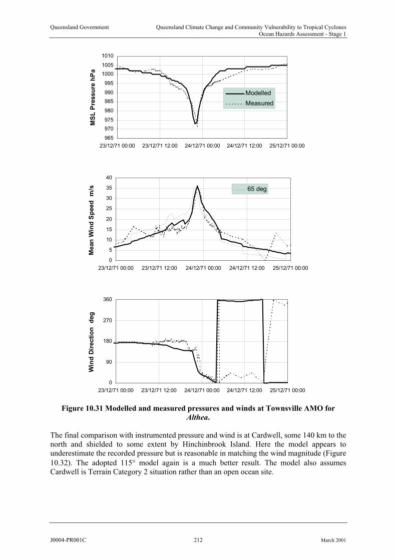
Queensland Government Queensland Climate Change and Community Vulnerability to Tropical CyclonesOcean Hazards Assessment - Stage 1
965
970
975
980
985
990
995
1000
1005
1010
23/12/71 00:00 23/12/71 12:00 24/12/71 00:00 24/12/71 12:00 25/12/71 00:00
MS
L P
ressu
re h
Pa
Modelled
Measured
0
5
10
15
20
25
30
35
40
23/12/71 00:00 23/12/71 12:00 24/12/71 00:00 24/12/71 12:00 25/12/71 00:00
Mean
Win
d S
peed
m
/s 65 deg
0
90
180
270
360
23/12/71 00:00 23/12/71 12:00 24/12/71 00:00 24/12/71 12:00 25/12/71 00:00
Win
d D
irecti
on
d
eg
Figure 1 .3 Modelled and measured pressures and winds at Townsville AMO for
Althea.
0 1
The final comparison with instrumented pressure and wind is at Cardwell, some 140 km to the north and shielded to some extent by Hinchinbrook Island. Here the model appears to underestimate the recorded pressure but is reasonable in matching the wind magnitude (Figure
10.32). The adopted 115 model again is a much better result. The model also assumesCardwell is Terrain Category 2 situation rather than an open ocean site.
J0004-PR001C 212 March 2001

Queensland Government Queensland Climate Change and Community Vulnerability to Tropical CyclonesOcean Hazards Assessment - Stage 1
980
985
990
995
1000
1005
1010
23/12/71 00:00 23/12/71 12:00 24/12/71 00:00 24/12/71 12:00 25/12/71 00:00
MS
L P
ressu
re h
Pa
Modelled
Measured
0
5
10
15
20
25
23/12/71 00:00 23/12/71 12:00 24/12/71 00:00 24/12/71 12:00 25/12/71 00:00
Mean
Win
d S
peed
m
/s 65 deg
0
90
180
270
360
23/12/71 00:00 23/12/71 12:00 24/12/71 00:00 24/12/71 12:00 25/12/71 00:00
Win
d D
irecti
on
d
eg
Figure 10.32 Modelled and measured pressures and winds at Cardwell for Althea.
J0004-PR001C 213 March 2001

Queensland Government Queensland Climate Change and Community Vulnerability to Tropical CyclonesOcean Hazards Assessment - Stage 1
10.4.3 Implications for Storm Surge Modelling
Figure 10.33 Modelled envelope of maximum winds and minimum pressure for Althea.
While there remain some minor inconsistencies between the modelled and measured wind and
pressure data, the parametric model with 115 maximum winds generally performs extremelywell. Some of these differences are in part due to errors in track, intensity and scale as well as the smoothing of those values within the model. Also, the "shrinking eye" undoubtedly created some localised variability as the storm neared the coast, which is currently beyond the capability of parametric models.
In Figure 10.33 below, the modelled envelope of maximum winds shows the extreme band of onshore winds that would have acted to produce this notable storm tide along the coast.
0
3 59 5 5
95
5
96
0
9 6 0
96 5
9 6 5
9 7 0
9 7 0
9 7 5
9 7 5
9 8 0
9 8 0
9 8 5
P a l l a r e n d a
T o w n s v i l l e
M a g n e t i c I s
T o w n s v i l l e A M O
T o o l a k e a
- 1 9 . 0 0
1 4 7 . 0 0
0
3 59 5 5
95
5
96
0
9 6 0
96 5
9 6 5
9 7 0
9 7 0
9 7 5
9 7 5
9 8 0
9 8 0
9 8 5
P a l l a r e n d a
T o w n s v i l l e
M a g n e t i c I s
T o w n s v i l l e A M O
T o o l a k e a
- 1 9 . 0 0
1 4 7 . 0 0
2 5
3
40
2 5
3
40
J0004-PR001C 214 March 2001

Queensland Government Queensland Climate Change and Community Vulnerability to Tropical CyclonesOcean Hazards Assessment - Stage 1
10.4.4 Tidal Modelling
0 4
Only five tidal constituents were available, but the modelled result is quite good as shown in Figure 10.34. The modelled tide is only about 0.05 m lower than the predicted low tide at 2130 UTC 23/12, close to the time of the peak surge. The following high tide is less accurate, being underpredicted by about 0.15 m.
-0.8
-0.6
-0.4
-0.2
0.0
0.2
0.4
0.6
0.8
1.0
1.2
23
00:00
23
06:00
23
12:00
23
18:00
24
00:00
24
06:00
24
12:00
24
18:00
25
00:00
Time UTC
Wate
r L
evel
(m
AH
D)
Predicted
Modelled
Figure 1 .3 Comparison of modelled and predicted tide at Townsville Harbour.
10.4.5 Storm Surge Modelling
A large number of individual tests were undertaken on the Althea storm tide event. Asdiscussed earlier, initial tests showed that the preferred windfield asymmetry assumption of a
65 or "front quadrant" max proved insufficient in matching the recorded surge magnitude andwas less successful in matching the recorded winds. Figure 10.35 presents the comparison between the front and rear quadrant wind assumptions on the modelled surge for the Townsville and Cleveland Bay grid domains. In the coarser Townsville grid, the surge is underpredicted by almost 24% and by 15% in the finer scale Cleveland Bay grid. This is a
very significant sensitivity to a single parameter and accordingly the rear quadrant 115 winds were retained.
Firstly, based on the standard 2D model, Figure 10.36 illustrates the surge-only build-up some6 h before the storm makes landfall on the 1 nmile Townsville grid. At this time, the invertedbarometer effect is clearly visible near the storm centre, beyond the continental shelf. At the coast, some water level increases are concentrated south of Cape Cleveland and CapeBowling Green. The shelf flow pattern indicates that a considerable northwards flow has already been initiated and strong currents are predicted on the outer edge of the Great BarrierReef. In Figure 10.37, the nearshore water levels and flows within the 0.2 nmile Cleveland
J0004-PR001C 215 March 2001
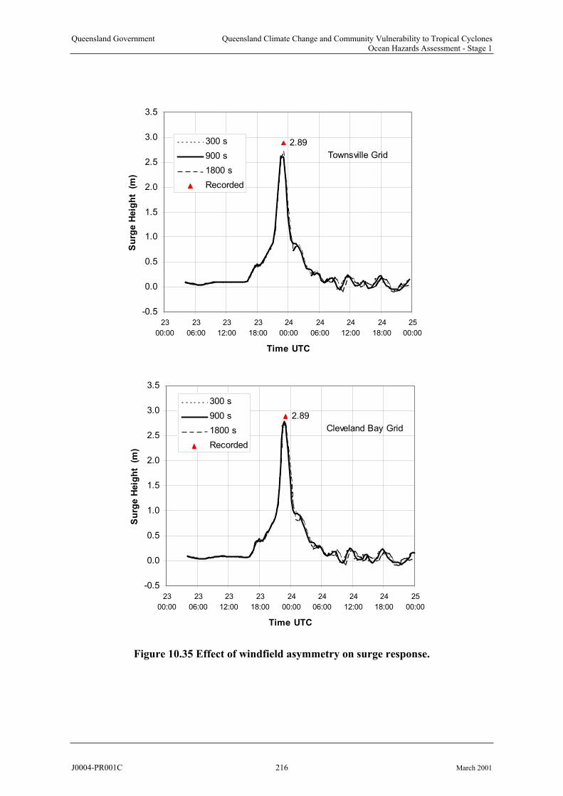
Queensland Government Queensland Climate Change and Community Vulnerability to Tropical CyclonesOcean Hazards Assessment - Stage 1
2.89
-0.5
0.0
0.5
1.0
1.5
2.0
2.5
3.0
3.5
23
00:00
23
06:00
23
12:00
23
18:00
24
00:00
24
06:00
24
12:00
24
18:00
25
00:00
Time UTC
Su
rge H
eig
ht
(m
)300 s
900 s
1800 s
Recorded
Townsville Grid
2.89
-0.5
0.0
0.5
1.0
1.5
2.0
2.5
3.0
3.5
23
00:00
23
06:00
23
12:00
23
18:00
24
00:00
24
06:00
24
12:00
24
18:00
25
00:00
Time UTC
Su
rge H
eig
ht
(m
)
300 s
900 s
1800 s
Recorded
Cleveland Bay Grid
Figure 1 .3 Effect of windfield asymmetry on surge response.0 5
J0004-PR001C 216 March 2001
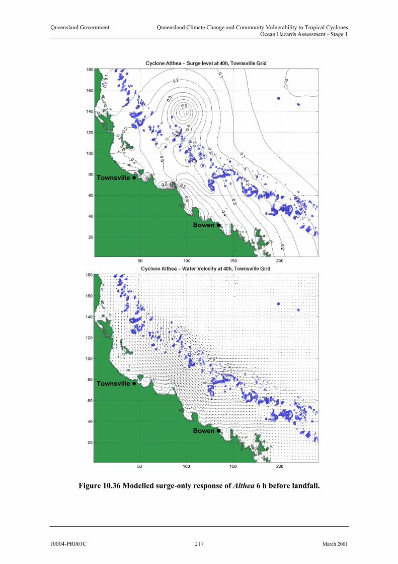
Queensland Government Queensland Climate Change and Community Vulnerability to Tropical CyclonesOcean Hazards Assessment - Stage 1
Townsville
Bowen
Townsville
Bowen
Figure 1 .3 Modelled surge-only response of Althea 6 h before landfall. 0 6
J0004-PR001C 217 March 2001
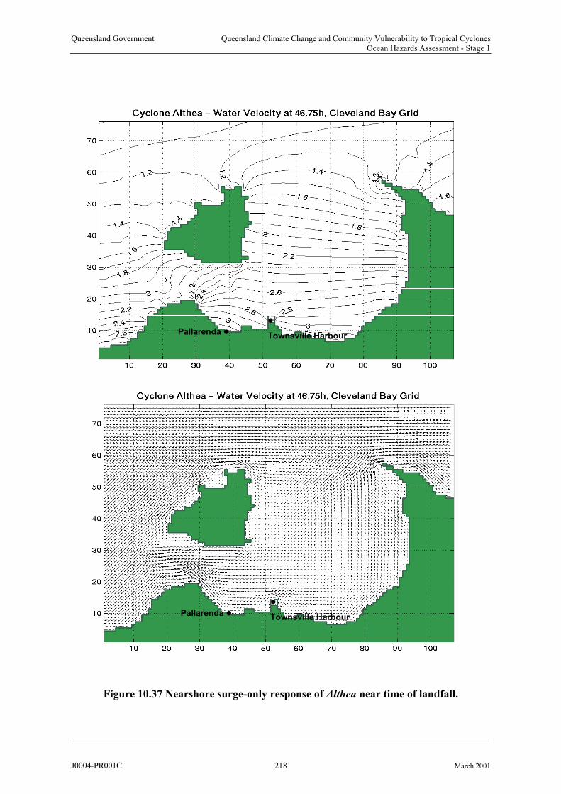
Queensland Government Queensland Climate Change and Community Vulnerability to Tropical CyclonesOcean Hazards Assessment - Stage 1
0 7
Townsville HarbourPallarenda
Townsville HarbourPallarenda
Figure 1 .3 Nearshore surge-only response of Althea near time of landfall.
J0004-PR001C 218 March 2001
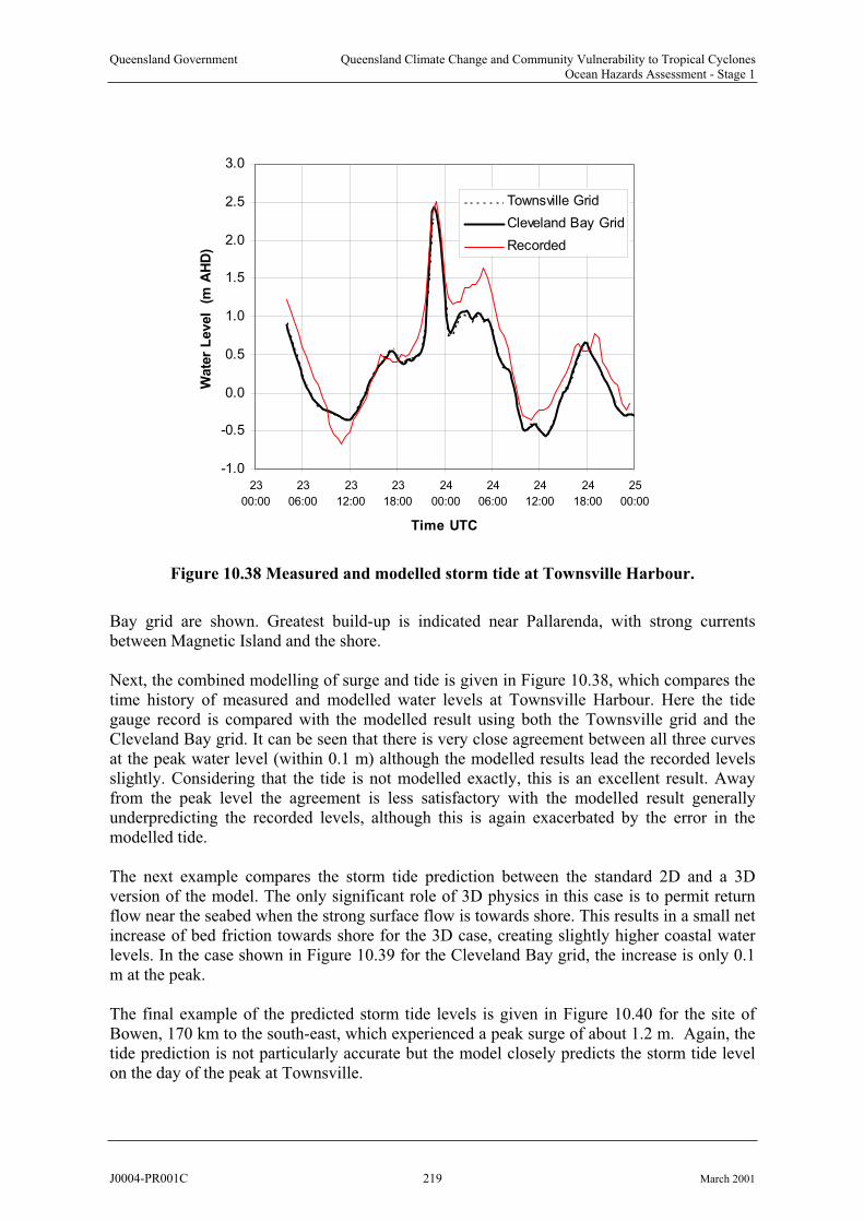
Queensland Government Queensland Climate Change and Community Vulnerability to Tropical CyclonesOcean Hazards Assessment - Stage 1
-1.0
-0.5
0.0
0.5
1.0
1.5
2.0
2.5
3.0
23
00:00
23
06:00
23
12:00
23
18:00
24
00:00
24
06:00
24
12:00
24
18:00
25
00:00
Time UTC
Wate
r L
evel
(m
AH
D)
Townsville Grid
Cleveland Bay Grid
Recorded
Figure 10.38 Measured and modelled storm tide at Townsville Harbour.
Bay grid are shown. Greatest build-up is indicated near Pallarenda, with strong currentsbetween Magnetic Island and the shore.
Next, the combined modelling of surge and tide is given in Figure 10.38, which compares thetime history of measured and modelled water levels at Townsville Harbour. Here the tide gauge record is compared with the modelled result using both the Townsville grid and theCleveland Bay grid. It can be seen that there is very close agreement between all three curvesat the peak water level (within 0.1 m) although the modelled results lead the recorded levels slightly. Considering that the tide is not modelled exactly, this is an excellent result. Away from the peak level the agreement is less satisfactory with the modelled result generallyunderpredicting the recorded levels, although this is again exacerbated by the error in themodelled tide.
The next example compares the storm tide prediction between the standard 2D and a 3D version of the model. The only significant role of 3D physics in this case is to permit return flow near the seabed when the strong surface flow is towards shore. This results in a small net increase of bed friction towards shore for the 3D case, creating slightly higher coastal waterlevels. In the case shown in Figure 10.39 for the Cleveland Bay grid, the increase is only 0.1 m at the peak.
The final example of the predicted storm tide levels is given in Figure 10.40 for the site of Bowen, 170 km to the south-east, which experienced a peak surge of about 1.2 m. Again, the tide prediction is not particularly accurate but the model closely predicts the storm tide level on the day of the peak at Townsville.
J0004-PR001C 219 March 2001

Queensland Government Queensland Climate Change and Community Vulnerability to Tropical CyclonesOcean Hazards Assessment - Stage 1
-1.0
-0.5
0.0
0.5
1.0
1.5
2.0
2.5
3.0
23
00:00
23
06:00
23
12:00
23
18:00
24
00:00
24
06:00
24
12:00
24
18:00
25
00:00
Time UTC
Wate
r L
evel
(m
AH
D)
2D
3D
Recorded
Figure 10.39 2D versus 3D model prediction for Althea.
-1.0
-0.5
0.0
0.5
1.0
1.5
23
00:00
23
06:00
23
12:00
23
18:00
24
00:00
24
06:00
24
12:00
24
18:00
25
00:00
Time UTC
Wate
r L
evel
(m
AH
D)
Bowen 2D
Recorded
Figure 10.40 Measured and modelled storm tide levels at Bowen for Althea.
J0004-PR001C 220 March 2001
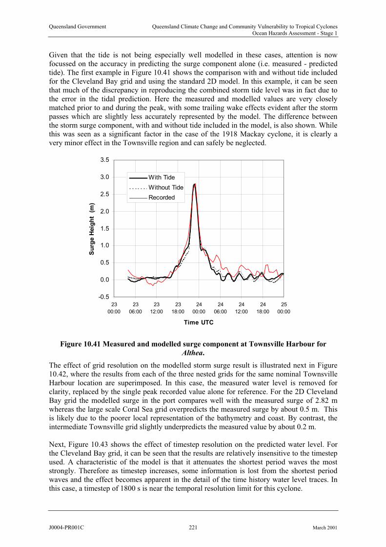
Queensland Government Queensland Climate Change and Community Vulnerability to Tropical CyclonesOcean Hazards Assessment - Stage 1
Given that the tide is not being especially well modelled in these cases, attention is nowfocussed on the accuracy in predicting the surge component alone (i.e. measured - predictedtide). The first example in Figure 10.41 shows the comparison with and without tide included for the Cleveland Bay grid and using the standard 2D model. In this example, it can be seen that much of the discrepancy in reproducing the combined storm tide level was in fact due to the error in the tidal prediction. Here the measured and modelled values are very closely matched prior to and during the peak, with some trailing wake effects evident after the stormpasses which are slightly less accurately represented by the model. The difference between the storm surge component, with and without tide included in the model, is also shown. Whilethis was seen as a significant factor in the case of the 1918 Mackay cyclone, it is clearly a very minor effect in the Townsville region and can safely be neglected.
-0.5
0.0
0.5
1.0
1.5
2.0
2.5
3.0
3.5
23
00:00
23
06:00
23
12:00
23
18:00
24
00:00
24
06:00
24
12:00
24
18:00
25
00:00
Time UTC
Su
rge H
eig
ht
(m
)
With Tide
Without Tide
Recorded
Figure 1 .4 Measured and modelled surge component at Townsville Harbour for
Althea.
0 1
The effect of grid resolution on the modelled storm surge result is illustrated next in Figure 10.42, where the results from each of the three nested grids for the same nominal TownsvilleHarbour location are superimposed. In this case, the measured water level is removed for clarity, replaced by the single peak recorded value alone for reference. For the 2D ClevelandBay grid the modelled surge in the port compares well with the measured surge of 2.82 mwhereas the large scale Coral Sea grid overpredicts the measured surge by about 0.5 m. Thisis likely due to the poorer local representation of the bathymetry and coast. By contrast, the intermediate Townsville grid slightly underpredicts the measured value by about 0.2 m.
Next, Figure 10.43 shows the effect of timestep resolution on the predicted water level. For the Cleveland Bay grid, it can be seen that the results are relatively insensitive to the timestepused. A characteristic of the model is that it attenuates the shortest period waves the moststrongly. Therefore as timestep increases, some information is lost from the shortest period waves and the effect becomes apparent in the detail of the time history water level traces. Inthis case, a timestep of 1800 s is near the temporal resolution limit for this cyclone.
J0004-PR001C 221 March 2001
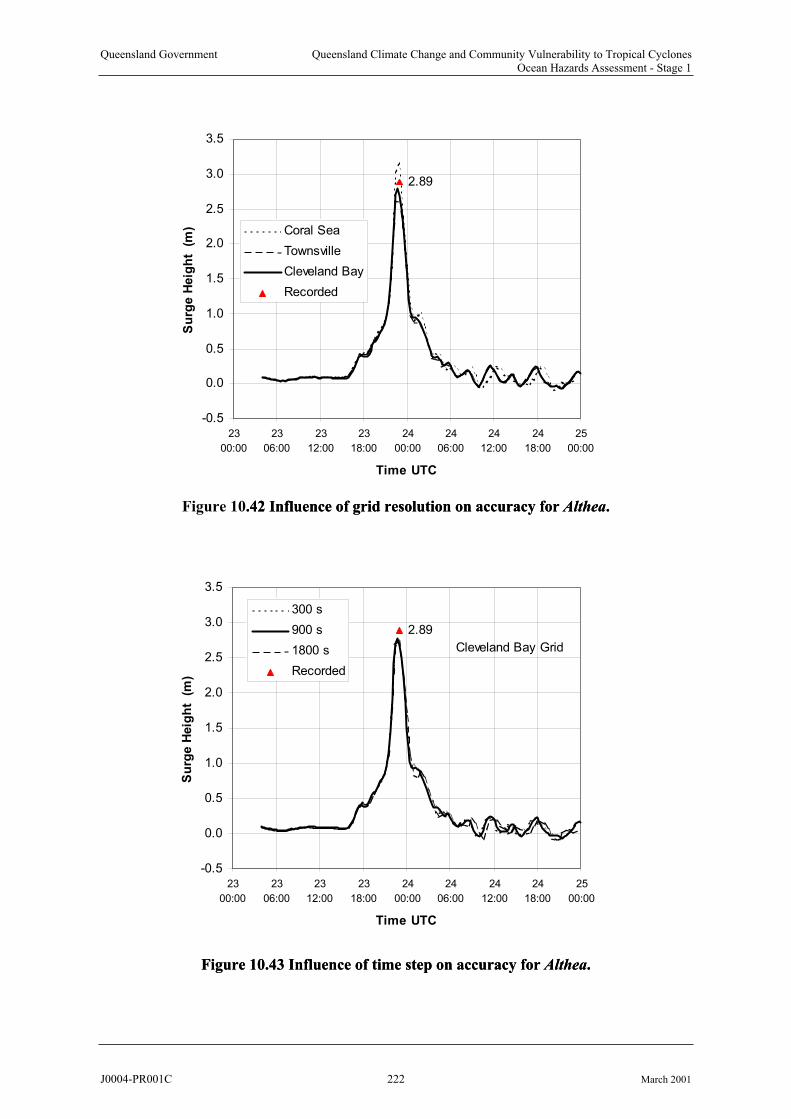
Queensland Government Queensland Climate Change and Community Vulnerability to Tropical CyclonesOcean Hazards Assessment - Stage 1
2.89
-0.5
0.0
0.5
1.0
1.5
2.0
2.5
3.0
3.5
23
00:00
23
06:00
23
12:00
23
18:00
24
00:00
24
06:00
24
12:00
24
18:00
25
00:00
Time UTC
Su
rge H
eig
ht
(m
) Coral Sea
Townsville
Cleveland Bay
Recorded
Figure 1 .4 Influence of grid resolution on accuracy for Althea..4 Influence of grid resolution on accuracy for Althea.0 22
2.89
-0.5
0.0
0.5
1.0
1.5
2.0
2.5
3.0
3.5
23
00:00
23
06:00
23
12:00
23
18:00
24
00:00
24
06:00
24
12:00
24
18:00
25
00:00
Time UTC
Su
rge H
eig
ht
(m
)
300 s
900 s
1800 s
Recorded
Cleveland Bay Grid
Figure 10.43 Influence of time step on accuracy for Althea.Figure 10.43 Influence of time step on accuracy for Althea.
J0004-PR001C 222 March 2001

Queensland Government Queensland Climate Change and Community Vulnerability to Tropical CyclonesOcean Hazards Assessment - Stage 1
As a guide, T/ t should be >= 20 (see Chapter 6), but the model can produce adequate results
for T/ t near or slightly below 10. During the 12 hours before landfall T/ t ranges fromapproximately 6 to 15 for the 1800 s timestep case.
A sensitivity test was also carried out to determine the influence of the Great Barrier Reef on predicted storm tide at Townsville. The model reef boundaries were removed and Althea re-modelled, yielding almost no difference in the predicted peak storm surge at the harbour gauge. This result is consistent with Sobey and Harper (1977) who concluded that the continental shelf at Townsville was sufficiently wide that the reef had essentially no impact, atleast for a storm track such as Althea. For tracks that are more southerly there may be an increased reef shielding effect.
An additional test was performed to gauge the influence of including the non-linear advectioncalculation in the model solution scheme (refer Appendix D). In this case, an additional test was run without non-linear advection and the results were essentially identical to the full non-linear case but with a 15% saving in computation time.
Finally, comparison between the final peak modelled values (Townsville and Cleveland Bay grids) and the estimated and/or measured peak storm surge magnitudes is shown in Figure 10.44. In this case, the debris line estimates from Figure 10.23 has been adjusted downward
by 0.5 m as a nominal allowance for wave setup and is shown with a 0.5 m error bar. The triangles represent the recorded levels at tide gauges. The solid line is the model result and indicates the peak surge magnitude was near Pallarenda at a level of 3.2 m. At Toolakea Beach, the location of the peak debris level of 3.6 m, the model predicts a 2.4 m surge. This ismuch lower than the observed debris line, even after wave setup and runup are considered. It suggests that Althea may have had a second wind maximum near Toolakea with significantly stronger winds than those predicted by the current single vortex model.
0.0
0.5
1.0
1.5
2.0
2.5
3.0
3.5
4.0
-150 -100 -50 0 50 100 150 200 250
Distance from Landfall km
Su
rge A
mp
litu
de
m
Figure 10.44 Comparison of modelled and measured alongshore surge profile for Althea.
J0004-PR001C 223 March 2001

Queensland Government Queensland Climate Change and Community Vulnerability to Tropical CyclonesOcean Hazards Assessment - Stage 1
10.4.6 References
BoM (1972) Report by Director of Meteorology on cyclone Althea. Bureau of Meteorology, Dept of Science, AGPS, Canberra, July.
BoM (1975) Tropical cyclones in the northern Australian regions. Meteorological Summary,Bureau of Meteorology, Dept of Science, AGPS, Canberra.
Broadbent G.J. (2000) Personal communication. Queensland Department of Transport.
Callaghan J. (1996) Tropical cyclones - analyses of the destructive wind zone. Proc. Conf. On Natural Disaster Reduction NDR 96, IEAust, Surfers Paradise, 29 Sept to 2 Oct, ISBN 0 85825 662 2, 341-345.
Callaghan J. (2000) Personal communication. Bureau of Meteorology, Queensland RegionalOffice.
Dunn S.L., Nielsen P., Madsen P.A. and Evans P. (2000) Wave diffraction and setup in jettied river entrances. Proc. 27th Intl. Conf. Coastal Engin., IEAust, 16 - 21st July, Sydney, ISBN 085825 722X.
Sobey R.J. and Harper B.A. (1977) Tropical cyclone surge penetration across the Great Barrier Reef, Proc 3rd Aust Conf Coastal and Ocean Eng, IEAust, Melbourne 1977, pp 58-63.
Harper B.A. and Holland G.J. (1999) An updated parametric model of the tropical cyclone. Proc. 23rd Conf. Hurricanes and Tropical Meteorology, AMS, Dallas, Texas, 10-15 Jan.
Powell M.D. and Houston S.H. (1996) Hurricane Andrew's landfall in South Florida. Part II: Surface wind fields and potential real-time applications. Weather and Forecasting, 11 (3), 329-349.
Stark K.P. (Ed.) (1972) Cyclone Althea part II - storm surges and coastal effects. James Cook
University of North Queensland, October.
Trollope D.H. (Ed.) (1972a) Cyclone Althea part I -buildings. James Cook University of
North Queensland, March.
J0004-PR001C 224 March 2001

Queensland Government Queensland Climate Change and Community Vulnerability to Tropical CyclonesOcean Hazards Assessment - Stage 1
10.5 Tropical Cyclone Ted December 1976 at Burketown
Tropical Cyclone Ted passed just westwards of Mornington Island and crossed the southern Gulf of Carpentaria coast on the afternoon of 19th December 1976, later passing directly overthe town of Burketown. It caused a very significant storm surge which in parts extended 20 km inland and up as far as the town itself, which is 40 km upstream of the Albert River mouth. Reports from nearby cattle stations confirmed extensive inundation of the low-lying coastal flats immediately to the east (Callaghan 2000). The nearest tidal readings wereunfortunately at Karumba, some 140 km to the east, although a single water level estimatefrom Mornington Island is available. Karumba was also close to being inundated, the peak levels reaching within about 1 m of the local ground levels.
10.5.1 Available Data
10.5.1.1 Storm Parameters
The National Climate Centre (NCC) official track for this event was obtained and consideredtogether with track modifications proposed by Callaghan south from Mornington Island which were used in an earlier storm surge assessment by Victory and Davis (1996). Bureau hardcopy records were also made available which included barographs at Mornington Island and Burketown, and observer notes with some estimated wind speeds and directions.Observer reports were also available from a number of cattle stations near Burketown, someof which reported passage of a calm and Augustus Downs provided a detailed pressure history. An anemograph from Port McArthur some 300 km to the NW was also considered. The limited electronic data available from NCC records were insufficient for the present purposes and accordingly most of the data was hand-digitised from the hardcopy records.
The cyclone was tracked by satellite during its early stages, as reported in an internal Bureau report, which details an eye diameter of 25 nmile visible through a series of NOAA5 orbits from 17/1041 UTC to 18/1136 UTC (refer Figure 10.45). After 18/2349 UTC it was reported that the eye was becoming obscured by cellular cloud and the storm appeared to bebroadening and weakening. This was at the time it was approaching Mornington Island and probably near the point of significant interaction between the outer circulation and the southwestern corner of the mainland. In spite of this intensity change assessment (i.e.weakening) the official pressure record shows a deepening system with the minimum pressuremaintained as a nominal 950 hPa, based on the Burketown reading in the eye some 10 h later and 30 km overland.
In hindsight therefore, the storm may well have been considerably more intense than the nominal 960 hPa from the official track during the early period of the 18th UTC when the eye was very clear. Although the images are not ideal, Callaghan (2000) advises that a Dvorak visible intensity estimate suggests that 930 hPa or even less may have been possible at that time. This would be consistent with the subsequent signs of weakening and the higherpressures at Mornington Island and Burketown. A synoptic view of the cyclone at landfall after Callaghan (2000) is given in Figure 10.46.
J0004-PR001C 225 March 2001

Queensland Government Queensland Climate Change and Community Vulnerability to Tropical CyclonesOcean Hazards Assessment - Stage 1
Figure 10.45 Satellite image of Ted (BoM photo)
Figure 10.46 Ted synoptic situation (after Callaghan 2000).
J0004-PR001C 226 March 2001
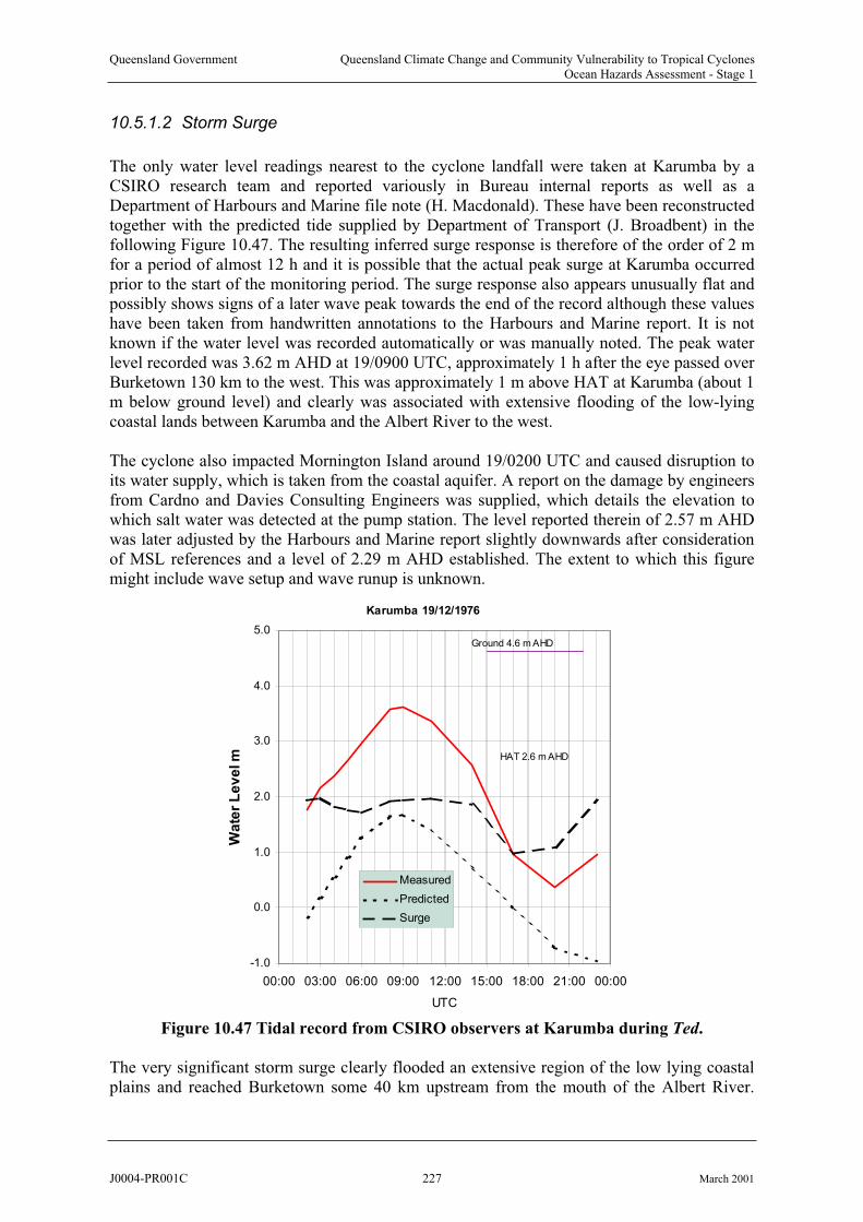
Queensland Government Queensland Climate Change and Community Vulnerability to Tropical CyclonesOcean Hazards Assessment - Stage 1
10.5.1.2 Storm Surge
The only water level readings nearest to the cyclone landfall were taken at Karumba by a CSIRO research team and reported variously in Bureau internal reports as well as aDepartment of Harbours and Marine file note (H. Macdonald). These have been reconstructed together with the predicted tide supplied by Department of Transport (J. Broadbent) in the following Figure 10.47. The resulting inferred surge response is therefore of the order of 2 mfor a period of almost 12 h and it is possible that the actual peak surge at Karumba occurredprior to the start of the monitoring period. The surge response also appears unusually flat and possibly shows signs of a later wave peak towards the end of the record although these values have been taken from handwritten annotations to the Harbours and Marine report. It is notknown if the water level was recorded automatically or was manually noted. The peak water level recorded was 3.62 m AHD at 19/0900 UTC, approximately 1 h after the eye passed over Burketown 130 km to the west. This was approximately 1 m above HAT at Karumba (about 1m below ground level) and clearly was associated with extensive flooding of the low-lying coastal lands between Karumba and the Albert River to the west.
The cyclone also impacted Mornington Island around 19/0200 UTC and caused disruption to its water supply, which is taken from the coastal aquifer. A report on the damage by engineers from Cardno and Davies Consulting Engineers was supplied, which details the elevation towhich salt water was detected at the pump station. The level reported therein of 2.57 m AHD was later adjusted by the Harbours and Marine report slightly downwards after consideration of MSL references and a level of 2.29 m AHD established. The extent to which this figure might include wave setup and wave runup is unknown.
Karumba 19/12/1976
-1.0
0.0
1.0
2.0
3.0
4.0
5.0
00:00 03:00 06:00 09:00 12:00 15:00 18:00 21:00 00:00
UTC
Wa
ter
Le
ve
l m
Measured
Predicted
Surge
HAT 2.6 m AHD
Ground 4.6 m AHD
Figure 10.47 Tidal record from CSIRO observers at Karumba during Ted.
The very significant storm surge clearly flooded an extensive region of the low lying coastal plains and reached Burketown some 40 km upstream from the mouth of the Albert River.
J0004-PR001C 227 March 2001
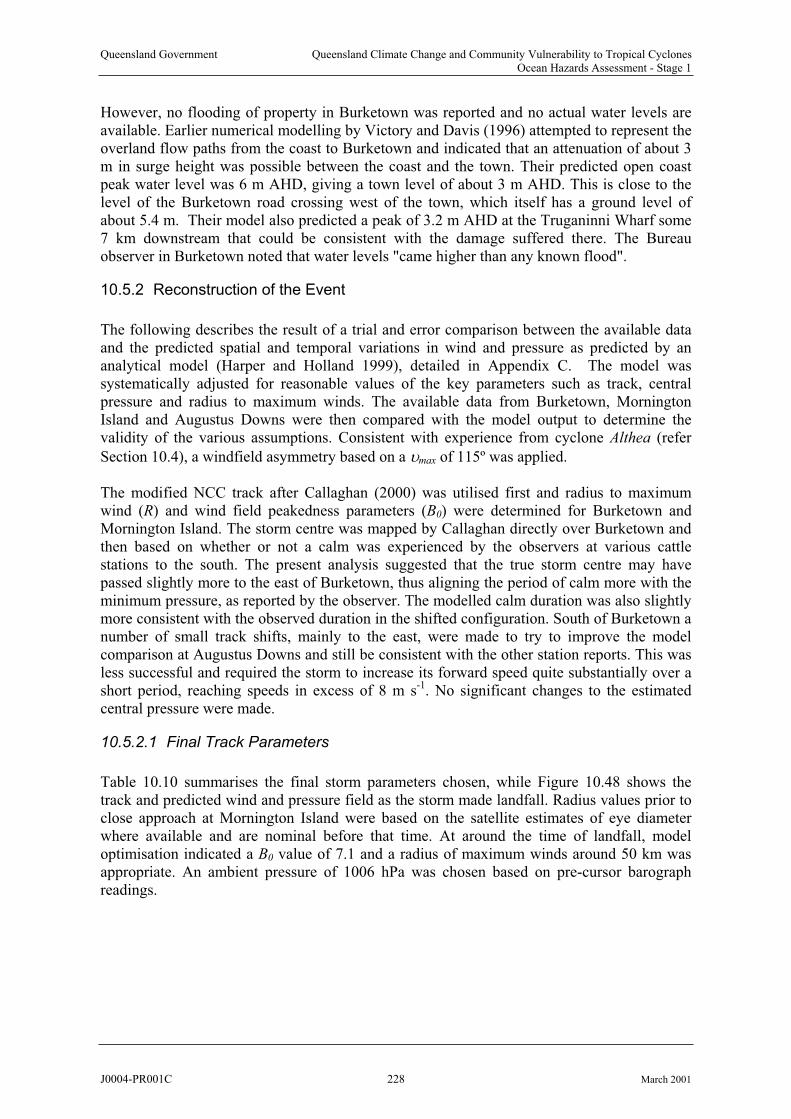
Queensland Government Queensland Climate Change and Community Vulnerability to Tropical CyclonesOcean Hazards Assessment - Stage 1
However, no flooding of property in Burketown was reported and no actual water levels are available. Earlier numerical modelling by Victory and Davis (1996) attempted to represent the overland flow paths from the coast to Burketown and indicated that an attenuation of about 3 m in surge height was possible between the coast and the town. Their predicted open coast peak water level was 6 m AHD, giving a town level of about 3 m AHD. This is close to the level of the Burketown road crossing west of the town, which itself has a ground level of about 5.4 m. Their model also predicted a peak of 3.2 m AHD at the Truganinni Wharf some7 km downstream that could be consistent with the damage suffered there. The Bureau observer in Burketown noted that water levels "came higher than any known flood".
10.5.2 Reconstruction of the Event
The following describes the result of a trial and error comparison between the available dataand the predicted spatial and temporal variations in wind and pressure as predicted by an analytical model (Harper and Holland 1999), detailed in Appendix C. The model was systematically adjusted for reasonable values of the key parameters such as track, central pressure and radius to maximum winds. The available data from Burketown, Mornington Island and Augustus Downs were then compared with the model output to determine the validity of the various assumptions. Consistent with experience from cyclone Althea (refer
Section 10.4), a windfield asymmetry based on a max of 115º was applied.
The modified NCC track after Callaghan (2000) was utilised first and radius to maximumwind (R) and wind field peakedness parameters (B0) were determined for Burketown andMornington Island. The storm centre was mapped by Callaghan directly over Burketown and then based on whether or not a calm was experienced by the observers at various cattle stations to the south. The present analysis suggested that the true storm centre may have passed slightly more to the east of Burketown, thus aligning the period of calm more with theminimum pressure, as reported by the observer. The modelled calm duration was also slightly more consistent with the observed duration in the shifted configuration. South of Burketown a number of small track shifts, mainly to the east, were made to try to improve the modelcomparison at Augustus Downs and still be consistent with the other station reports. This was less successful and required the storm to increase its forward speed quite substantially over a short period, reaching speeds in excess of 8 m s-1. No significant changes to the estimatedcentral pressure were made.
10.5.2.1 Final Track Parameters
Table 10.10 summarises the final storm parameters chosen, while Figure 10.48 shows the track and predicted wind and pressure field as the storm made landfall. Radius values prior toclose approach at Mornington Island were based on the satellite estimates of eye diameterwhere available and are nominal before that time. At around the time of landfall, modeloptimisation indicated a B0 value of 7.1 and a radius of maximum winds around 50 km wasappropriate. An ambient pressure of 1006 hPa was chosen based on pre-cursor barograph readings.
J0004-PR001C 228 March 2001

Queensland Government Queensland Climate Change and Community Vulnerability to Tropical CyclonesOcean Hazards Assessment - Stage 1
Table 10.10 Adopted hindcast parameters for tropical cyclone Ted.
Track Fix Speed Bearing CentralPressure
Radius Peakedness
Lat Long Vfm fm p0 B0
m s-1 hPa km
15-Dec-1976 23:00 -12.6 140.5 2.1 256 1005 100 7.1
16-Dec-1976 05:00 -12.7 140.1 2.1 256 1001 100 7.1
16-Dec-1976 11:00 -12.8 139.7 2.1 256 997 100 7.1
16-Dec-1976 17:00 -12.9 139.3 1.6 251 994 100 7.1
16-Dec-1976 23:00 -13.0 139.0 270 1001.0 990 7.1
17-Dec-1976 05:00 -13.0 1.1 982138.8 243 82 7.1
17-Dec-1976 11:00 -13.1 138.6 1.0 270 974 64 7.1
17-Dec-1976 17:00 -13.1 138.4 1.6 969 7.1251 46
-13.2 3.7 213 964 28 7.1
18-Dec-1976 02:00 -13.5 137.9 3.7 963213 28 7.1
18-Dec-1976 05:00 -13.8 137.7 4.2 166 962 28 7.1
18-Dec-1976 08:00 -14.2 961137.8 5.2 169 28 7.1
-14.7 137.9 4.1 151 960 28 7.1
18-Dec-1976 17:00 -15.4 138.3 4.1 151 955 35 7.1
18-Dec-1976 23:00 -16.1 138.7 6.0 162 950 42 7.1
19-Dec-1976 02:15 -16.7 138.9 6.0 161 950 45 7.1
19-Dec-1976 05:00 -17.2 139.1 4.1 136 950 48 7.1
19-Dec-1976 10:15 -17.7 139.6 4.5 136 948 54 7.1
19-Dec-1976 13:45 -18.1 140.0 6.8 144 955 55 7.1
19-Dec-1976 15:00 -18.4 140.2 8.1 105 965 55 7.1
19-Dec-1976 16:30 -18.5 140.6 8.5 136 970 55 7.1
19-Dec-1976 18:00 -18.8 140.9 6.8 205 970 55 7.1
19-Dec-1976 20:00 -19.2 140.7 3.2 162 980 55 7.1
19-Dec-1976 23:00 -19.5 140.8 1.5 7.1180 985 55
19-Dec-1976 23:30 -19.5 140.8 1.5 180 985 55 7.1
20-Dec-1976 05:00 -19.8 140.8 1.5 180 988 55 7.1
20-Dec-1976 11:00 -20.1 140.8 1.5 180 992 55 7.1
20-Dec-1976 17:00 -20.4 140.8 1.5 180 996 55 7.1
20-Dec-1976 23:00 -20.7 140.8 1.5 180 1000 55 7.1
Time R
UTC
17-Dec-1976 23:00 138.1
18-Dec-1976 11:00
10.5.2.2 Comparison of Measured and Modelled Storm Parameters
The Burketown Post Office barograph was digitised and pressures adjusted to match the annotated chart time-check pressures. [Callaghan (2000) notes that it was routine procedure to set the barograph approximately +10 hPa relative to the actual pressure during summer to provide a safety factor against "bottoming out" at the 950 hPa chart limit in the event of a close cyclone.] The minimum MSL pressure recorded at Burketown on this basis was 948.6 hPa and, based on the observer notes, occurred during a calm which lasted 1.5 h. No windspeed or direction data is available. The digitised pressure trace together with the optimisedmodel fit is reproduced here as Figure 10.49 indicating a peak mean wind of about 30 m s-1.
J0004-PR001C 229 March 2001
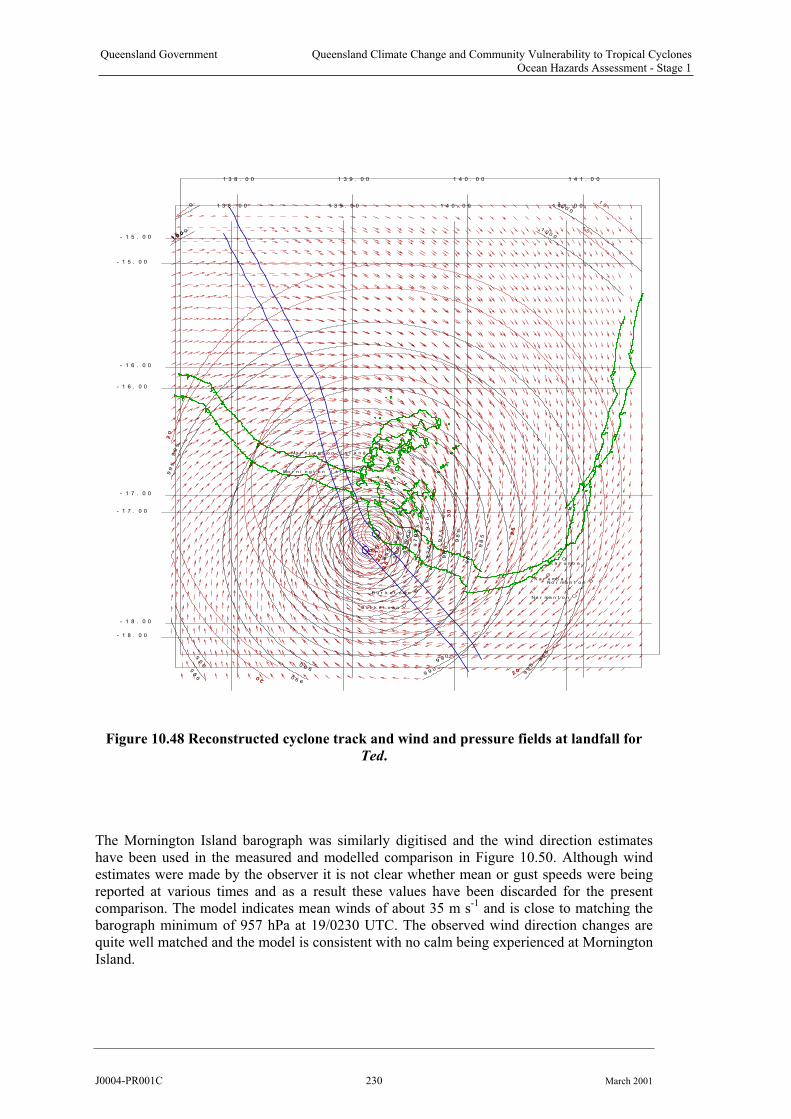
Queensland Government Queensland Climate Change and Community Vulnerability to Tropical CyclonesOcean Hazards Assessment - Stage 1
15
95
5
96
0
96
5 97
0
97
5
98
0
98
5
9 9 0
990 99
5
99
5
99
51
0 00
0
K a r u mb a
Mo r n i n g t o n I s l a n d
B u r k e t o w n
N o r ma n t o n
- 1 8 . 0 0
- 1 7 . 0 0
- 1 6 . 0 0
- 1 5 . 0 0
1 3 8 . 0 0 1 3 9 . 0 0 1 4 0 . 0 0 1 4 1 . 0 0
15
95
5
96
0
96
5 97
0
97
5
98
0
98
5
9 9 0
990 99
5
99
5
99
5
10 0
00
K a r u mb a
Mo r n i n g t o n I s l a n d
B u r k e t o w n
N o r ma n t o n
- 1 8 . 0 0
- 1 7 . 0 0
- 1 6 . 0 0
- 1 5 . 0 0
1 3 8 . 0 0 1 3 9 . 0 0 1 4 0 . 0 0 1 4 1 . 0 0
51
0
15
15
20
20
20
20
25
25
30
10
51
0
15
15
20
20
20
20
25
25
30
10
00
Figure 1 .4 Reconstructed cyclone track and wind and pressure fields at landfall for
Ted.
0 8
The Mornington Island barograph was similarly digitised and the wind direction estimateshave been used in the measured and modelled comparison in Figure 10.50. Although wind estimates were made by the observer it is not clear whether mean or gust speeds were beingreported at various times and as a result these values have been discarded for the presentcomparison. The model indicates mean winds of about 35 m s and is close to matching the barograph minimum of 957 hPa at 19/0230 UTC. The observed wind direction changes are quite well matched and the model is consistent with no calm being experienced at Mornington Island.
-1
J0004-PR001C 230 March 2001
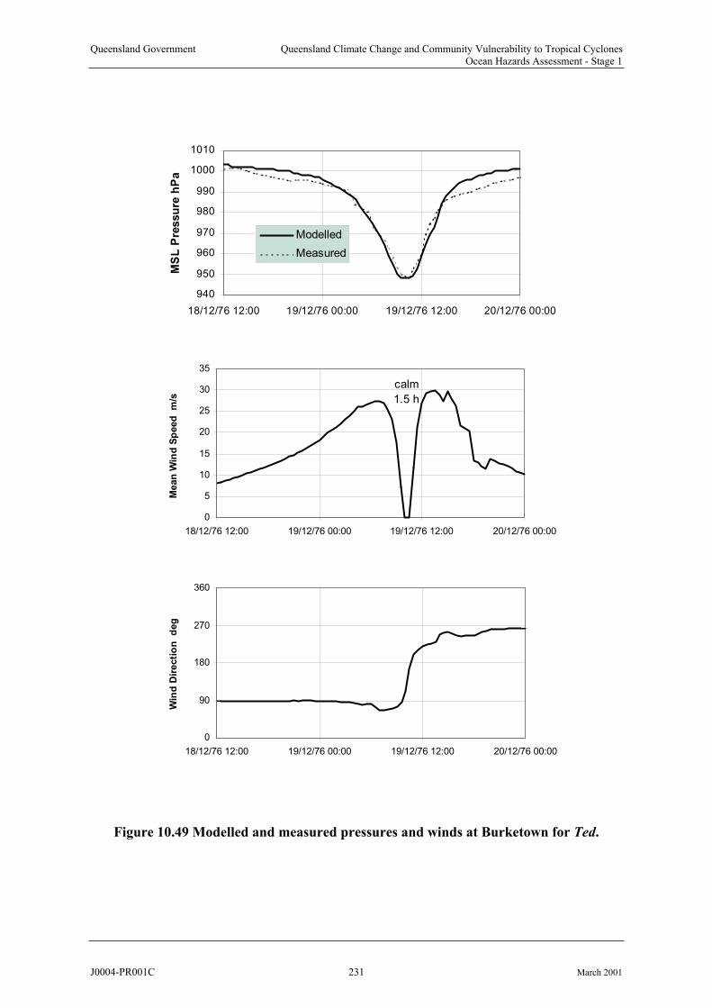
Queensland Government Queensland Climate Change and Community Vulnerability to Tropical CyclonesOcean Hazards Assessment - Stage 1
940
950
960
970
980
990
1000
1010
18/12/76 12:00 19/12/76 00:00 19/12/76 12:00 20/12/76 00:00
MS
L P
ressu
re h
Pa
Modelled
Measured
0
5
10
15
20
25
30
35
18/12/76 12:00 19/12/76 00:00 19/12/76 12:00 20/12/76 00:00
Mean
Win
d S
peed
m/s
calm
1.5 h
0
90
180
270
360
18/12/76 12:00 19/12/76 00:00 19/12/76 12:00 20/12/76 00:00
Win
d D
irecti
on
deg
Figure 10.49 Modelled and measured pressures and winds at Burketown for Ted.
J0004-PR001C 231 March 2001
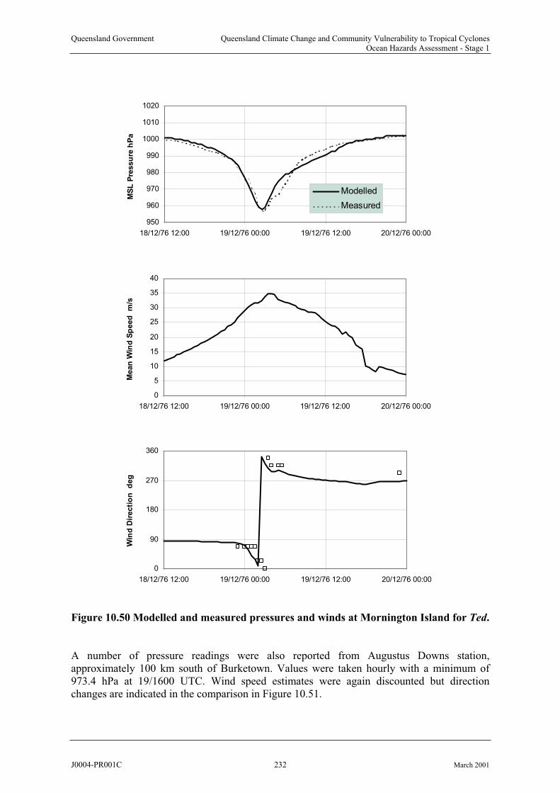
Queensland Government Queensland Climate Change and Community Vulnerability to Tropical CyclonesOcean Hazards Assessment - Stage 1
950
960
970
980
990
1000
1010
1020
18/12/76 12:00 19/12/76 00:00 19/12/76 12:00 20/12/76 00:00
MS
L P
ressu
reh
Pa
Modelled
Measured
0
5
10
15
20
25
30
35
40
18/12/76 12:00 19/12/76 00:00 19/12/76 12:00 20/12/76 00:00
Mean
Win
d S
peed
m/s
0
90
180
270
360
18/12/76 12:00 19/12/76 00:00 19/12/76 12:00 20/12/76 00:00
Win
d D
irecti
on
deg
Figure 10.50 Modelled and measured pressures and winds at Mornington Island for Ted.
A number of pressure readings were also reported from Augustus Downs station, approximately 100 km south of Burketown. Values were taken hourly with a minimum of 973.4 hPa at 19/1600 UTC. Wind speed estimates were again discounted but direction changes are indicated in the comparison in Figure 10.51.
J0004-PR001C 232 March 2001
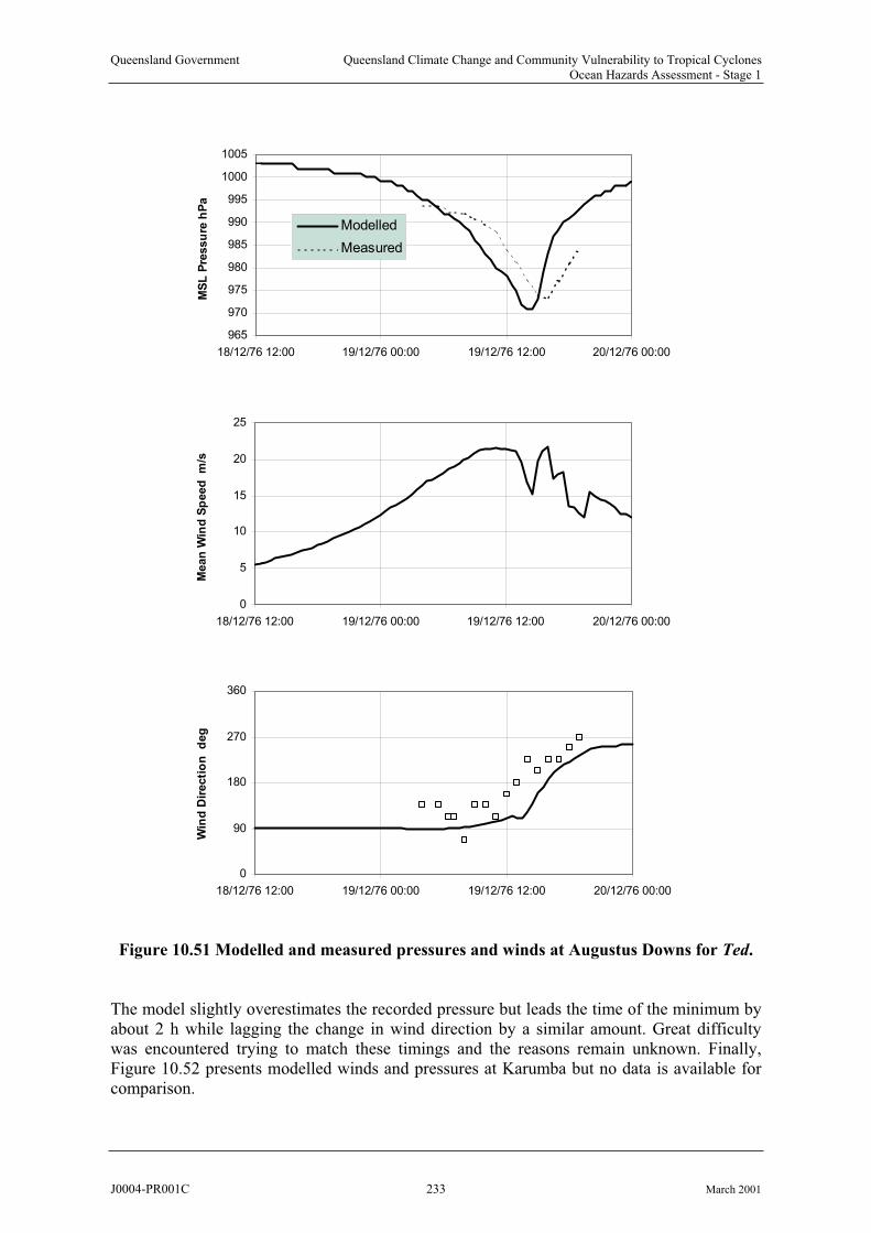
Queensland Government Queensland Climate Change and Community Vulnerability to Tropical CyclonesOcean Hazards Assessment - Stage 1
965
970
975
980
985
990
995
1000
1005
18/12/76 12:00 19/12/76 00:00 19/12/76 12:00 20/12/76 00:00
MS
L P
ressu
reh
Pa
Modelled
Measured
0
5
10
15
20
25
18/12/76 12:00 19/12/76 00:00 19/12/76 12:00 20/12/76 00:00
Mean
Win
d S
peed
m/s
0
90
180
270
360
18/12/76 12:00 19/12/76 00:00 19/12/76 12:00 20/12/76 00:00
Win
d D
irecti
on
deg
Figure 10.51 Modelled and measured pressures and winds at Augustus Downs for Ted.
The model slightly overestimates the recorded pressure but leads the time of the minimum by about 2 h while lagging the change in wind direction by a similar amount. Great difficulty was encountered trying to match these timings and the reasons remain unknown. Finally, Figure 10.52 presents modelled winds and pressures at Karumba but no data is available forcomparison.
J0004-PR001C 233 March 2001
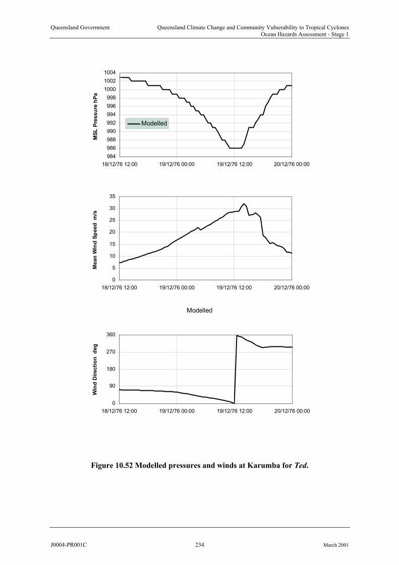
Queensland Government Queensland Climate Change and Community Vulnerability to Tropical CyclonesOcean Hazards Assessment - Stage 1
984
986
988
990
992
994
996
998
1000
1002
1004
18/12/76 12:00 19/12/76 00:00 19/12/76 12:00 20/12/76 00:00
MS
L P
ressu
reh
Pa
Modelled
0
5
10
15
20
25
30
35
18/12/76 12:00 19/12/76 00:00 19/12/76 12:00 20/12/76 00:00
Mean
Win
d S
peed
m/s
Modelled
0
90
180
270
360
18/12/76 12:00 19/12/76 00:00 19/12/76 12:00 20/12/76 00:00
Win
d D
irecti
on
deg
0 2Figure 1 .5 Modelled pressures and winds at Karumba for Ted.
J0004-PR001C 234 March 2001

Queensland Government Queensland Climate Change and Community Vulnerability to Tropical CyclonesOcean Hazards Assessment - Stage 1
10.5.3 Implications for Storm Surge Modelling
The intensity of cyclone Ted before its close approach to Mornington Island remainsunknown, but the model optimisation is at least consistent with the observed broadening of the eye at that time, producing a relatively large scale storm circulation as a result. The qualityof recorded water levels and an absence of objective wind data leave a relatively large marginof error in predicting the peak surge.
In Figure 10.53 below, the modelled envelope of maximum winds shows the extreme band of onshore winds that would have acted to produce an extreme storm tide along the coast.
25
95
0
9 5 5
960 9
60
96
5
96
5
97
0 097
5
97
5
98
0
98
0
98
5
98
5
99
0
99
0
99
5
99
5
10
00
K a r u mb a
Mo r n i n g t o n I s l a n d
B u r k e t o w n
N o r ma n t o n
- 1 8 . 0 0
- 1 7 . 0 0
- 1 6 . 0 0
- 1 5 . 0 0
25
95
0
9 5 5
960 9
60
96
5
96
5
97
0 097
5
97
5
98
0
98
0
98
5
98
5
99
0
99
0
99
5
99
5
10
00
K a r u mb a
Mo r n i n g t o n I s l a n d
B u r k e t o w n
N o r ma n t o n
- 1 8 . 0 0
- 1 7 . 0 0
- 1 6 . 0 0
- 1 5 . 0 0
20
20
25
30
30
35
3 5
97
20
20
25
30
30
35
3 5
97
Figure 10.53 Modelled envelope of maximum winds and minimum pressure for Ted.
J0004-PR001C 235 March 2001
Queensland Government Queensland Climate Change and Community Vulnerability to Tropical CyclonesOcean Hazards Assessment - Stage 1
10.5.4 Tidal Modelling
The Arafura Sea and Gulf of Carpentaria is a unique part of the world oceans. The area issemi-enclosed and covers many hundreds of thousands of square kilometres of ocean that is less than 70 m deep. It is one of the world's largest sinks of tidal energy due to bottom friction. The region has both large diurnal and semi-diurnal tides. Semi-diurnal tides aredominant in the northern parts of the region while diurnal tides are relatively large in thesouthern part of the gulf. Non-tidally induced water height variations are also significant in this region. Oceanic water level fluctuations and wind stress are the major contributors tothese variations. Both these mechanisms have a strong seasonal signal, and significant changes in water level (e.g. 0.3 - 1 m) have been observed over short periods with changing wind conditions. The coastal areas of the southern and southeastern part of the gulf are also usual. This part of the coast contains large areas of tidal flats which in places extend sometens of kilometres inland. As a result there are many hundreds of square kilometres of land potentially susceptible to storm surge inundation.
Because of the regional complexity, the hindcast modelling of Ted has been undertaken using an existing outer grid (5 nmile) that completely covers the Gulf of Carpentaria and theshallower parts of the Arafura Sea. A second smaller grid with a resolution of 0.5 nmile was especially generated for the area southeast of Mornington Island but does have known errors both in bathymetry and land elevation. Land elevations were taken from the GTOPO30 global database and individual grid points from this database were adjusted so that the minimumelevation was 2.5 m above AHD. This gives only a very approximate representation of the floodable land in the region.
Tidal boundary conditions were then applied to the Gulf of Carpentaria grid using only thefive constituents available. These are not sufficient for accurately reproducing the tide at Karumba or Mornington Island. At the time of Ted's landfall the modelled high tide at Karumba was 0.5 m below predicted (refer Figure 10.54). At Mornington Island however, the model gives reasonable agreement at high tide but underpredicts the low tide (Figure 10.55).
A significant amount of work is indicated to improve the representation of the Gulf of Carpentaria region and to properly calibrate a tidal model. The present study has only been able to draw upon readily available sources of information.
10.5.5 Storm Surge Modelling
Because of the poor tide representation, the surge-only response without any tidal input is discussed initially. Discussion on water levels over flooded land is deferred to the tide-included case, although the levels are somewhat in error, because the extent of flooding critically depends on an absolute water level.
An overall view of the Gulf of Carpentaria modelled response to Ted is shown in Figure 10.56, approximately at the time of passage over Burketown. The largest surge build-up is indicated in the region between Karumba and Burketown, which is consistent with theexperience of the various landowners.
J0004-PR001C 236 March 2001

Queensland Government Queensland Climate Change and Community Vulnerability to Tropical CyclonesOcean Hazards Assessment - Stage 1
-1.5
-1.0
-0.5
0.0
0.5
1.0
1.5
2.0
18
00:00
18
06:00
18
12:00
18
18:00
19
00:00
19
06:00
19
12:00
19
18:00
20
00:00
20
06:00
20
12:00
20
18:00
21
00:00
Time UTC
Wate
r L
evel
(mA
HD
)
Predicted
Modelled 5 nmile
Figure 10.54 Modelled and measured tides at Karumba for Ted.
-1.5
-1.0
-0.5
0.0
0.5
1.0
1.5
18
00:00
18
06:00
18
12:00
18
18:00
19
00:00
19
06:00
19
12:00
19
18:00
20
00:00
20
06:00
20
12:00
20
18:00
21
00:00
Time UTC
Wate
r L
evel (m
AH
D)
Predicted
Modelled 5 nmile
Figure 10.55 Measured and modelled tides at Mornington Island for Ted.
J0004-PR001C 237 March 2001
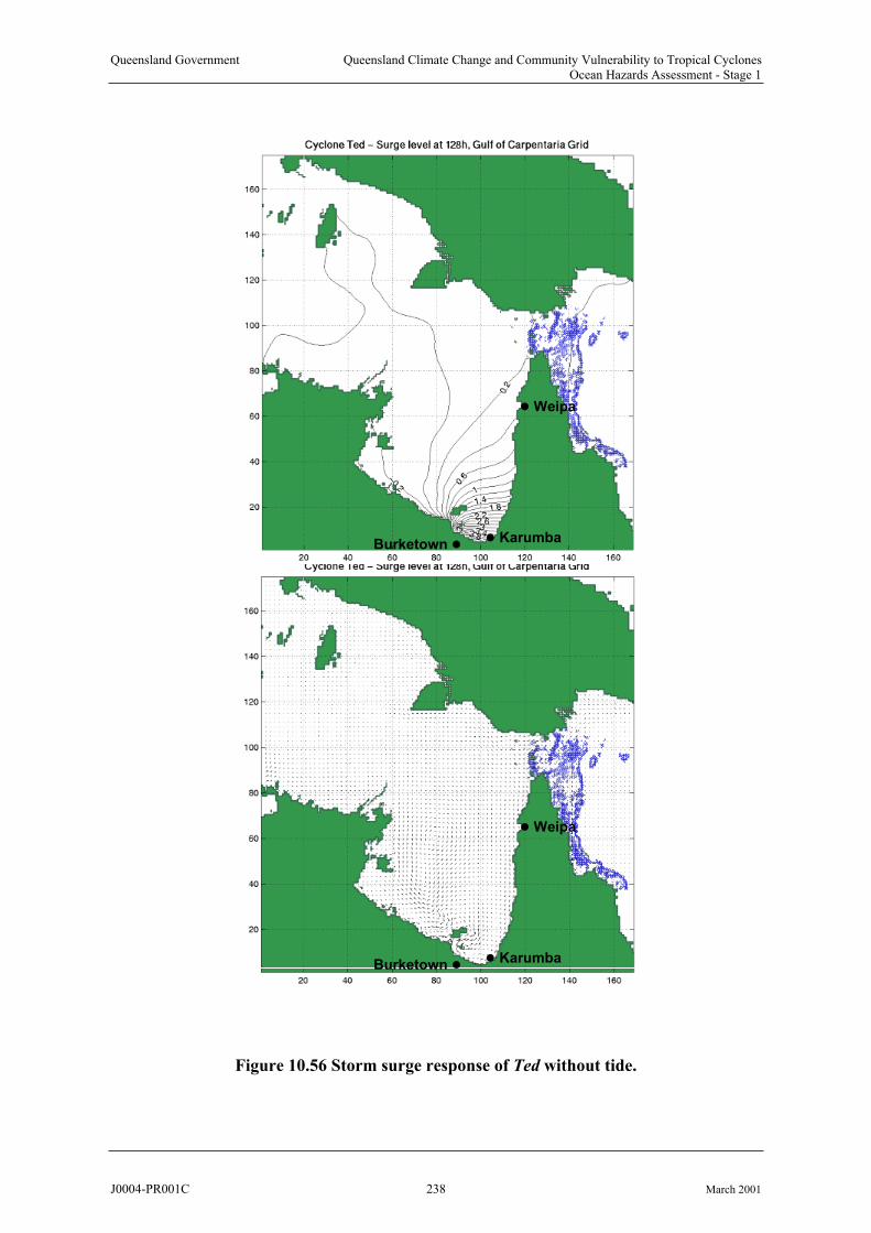
Queensland Government Queensland Climate Change and Community Vulnerability to Tropical CyclonesOcean Hazards Assessment - Stage 1
Karumba
Weipa
Burketown
Karumba
Weipa
Burketown
Figure 10.56 Storm surge response of Ted without tide.
J0004-PR001C 238 March 2001

Queensland Government Queensland Climate Change and Community Vulnerability to Tropical CyclonesOcean Hazards Assessment - Stage 1
-1.0
0.0
1.0
2.0
3.0
4.0
18
00:00
18
06:00
18
12:00
18
18:00
19
00:00
19
06:00
19
12:00
19
18:00
20
00:00
20
06:00
20
12:00
20
18:00
21
00:00
Time UTC
Su
rge H
eig
ht
(m)
Modelled 5 nmile
Modelled 0.5 nmile
Measured
Figure 1 .5 Measured and modelled surge height at Karumba for Ted.0 7
-0.5
0.0
0.5
1.0
1.5
2.0
2.5
3.0
3.5
18 00:00 18 06:00 18 12:00 18 18:00 19 00:00 19 06:00 19 12:00 19 18:00 20 00:00
Time UTC
Su
rge H
eig
ht
(m)
Modelled 5 nmile
Modelled 0.5 nmile
Estimated
Figure 10.58 Measured and modelled surge height at Mornington Island for Ted.
J0004-PR001C 239 March 2001
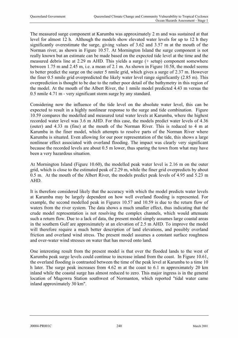
Queensland Government Queensland Climate Change and Community Vulnerability to Tropical CyclonesOcean Hazards Assessment - Stage 1
The measured surge component at Karumba was approximately 2 m and was sustained at that level for almost 12 h. Although the models show elevated water levels for up to 12 h they significantly overestimate the surge, giving values of 3.62 and 3.57 m at the mouth of the Norman river, as shown in Figure 10.57. At Mornington Island the surge component is not really known but an estimate can be made based on the expected tide level at the time and the measured debris line at 2.29 m AHD. This yields a surge (+ setup) component somewherebetween 1.75 m and 2.45 m, i.e. a mean of 2.1 m. As shown in Figure 10.58, the model seemsto better predict the surge on the outer 5 nmile grid, which gives a surge of 2.37 m. However the finer 0.5 nmile grid overpredicted the likely water level range significantly (2.85 m). This overprediction is thought to be due to the rather poor detail of the bathymetry in this region of the model. At the mouth of the Albert River, the 1 nmile model predicted 4.43 m versus the 0.5 nmile 4.71 m - very significant storm surge by any standard.
Considering now the influence of the tide level on the absolute water level, this can beexpected to result in a highly nonlinear response to the surge and tide combination. Figure 10.59 compares the modelled and measured total water levels at Karumba, where the highestrecorded water level was 3.6 m AHD. For this case, the models predict water levels of 4.36 (outer) and 4.33 m (fine) at the mouth of the Norman River. This is reduced to 4 m at Karumba in the finer model, which attempts to resolve parts of the Norman River whereKarumba is situated. Even allowing for our poor representation of the tide, this shows a large nonlinear effect associated with overland flooding. The impact was clearly very significantbecause the recorded levels are about 0.5 m lower, thus sparing the town from what may have been a very hazardous situation.
At Mornington Island (Figure 10.60), the modelled peak water level is 2.16 m on the outer grid, which is close to the estimated peak of 2.29 m, while the finer grid overpredicts by about0.5 m. At the mouth of the Albert River, the models predict peak levels of 4.95 and 5.23 mAHD.
It is therefore considered likely that the accuracy with which the model predicts water levels at Karumba may be largely dependent on how well overland flooding is represented. For example, the second modelled peak in Figures 10.57 and 10.59 is due to the return flow of waters from the river system. The data shows a much smaller effect, thus indicating that the crude model representation is not resolving the complex channels, which would attenuate such a return flow. Due to a lack of data, the present model simply assumes large coastal areasin the southern Gulf are approximately at an elevation of 2.5 m AHD. To improve the modelwill therefore require a much better description of land elevations, and possibly overland friction and overland wind stress. The present model assumes a constant surface roughnessand over-water wind stresses on water that has moved onto land.
One interesting result from the present model is that over the flooded lands to the west ofKarumba peak surge levels could continue to increase inland from the coast. In Figure 10.61, the overland flooding is contrasted between the time of the peak level at Karumba to a time 10 h later. The surge peak increases from 4.62 m at the coast to 6.1 m approximately 20 kminland while the coastal surge has almost reduced to zero. This major ingress is in the generallocation of Magowra Station southwest of Normanton, which reported "tidal water cameinland approximately 30 km".
J0004-PR001C 240 March 2001
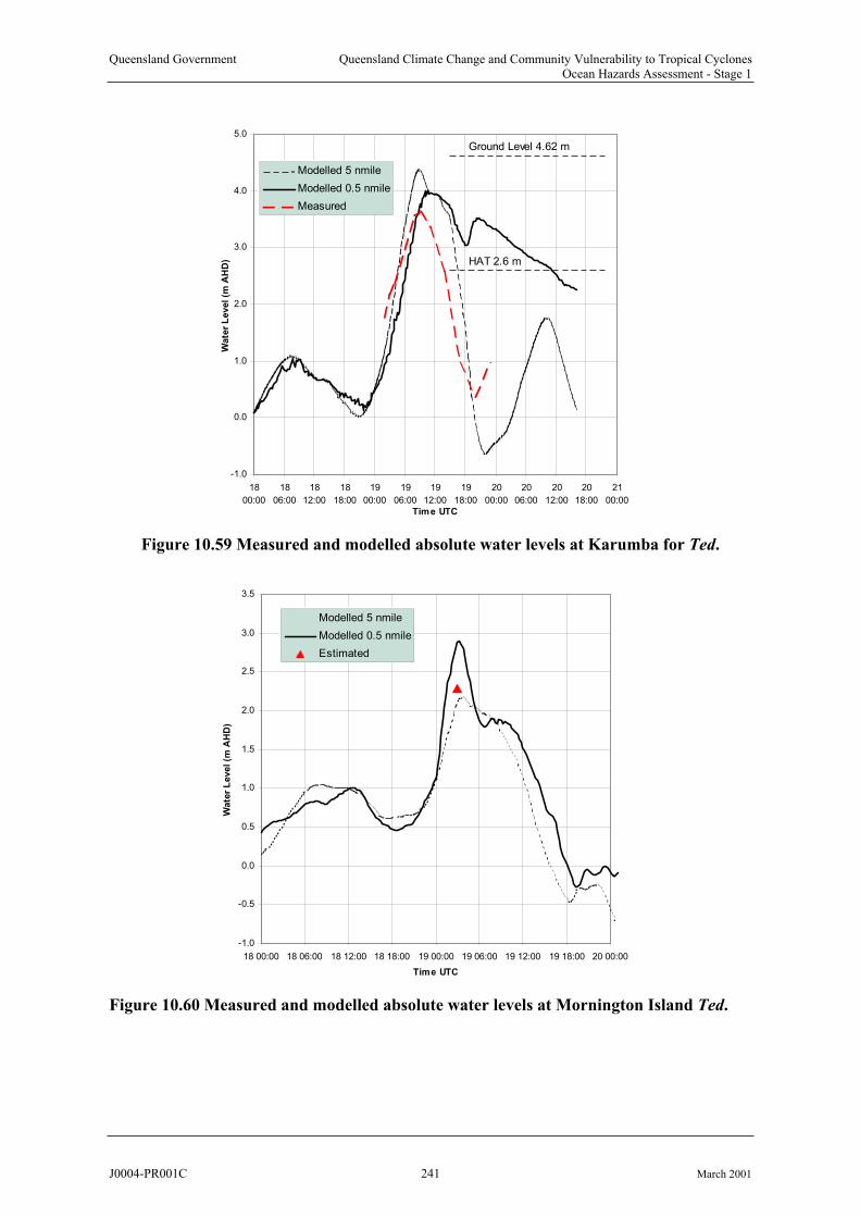
Queensland Government Queensland Climate Change and Community Vulnerability to Tropical CyclonesOcean Hazards Assessment - Stage 1
-1.0
0.0
1.0
2.0
3.0
4.0
5.0
18
00:00
18
06:00
18
12:00
18
18:00
19
00:00
19
06:00
19
12:00
19
18:00
20
00:00
20
06:00
20
12:00
20
18:00
21
00:00
Time UTC
Wate
r L
evel (m
AH
D)
Modelled 5 nmile
Modelled 0.5 nmile
Measured
Ground Level 4.62 m
HAT 2.6 m
Figure 10.59 Measured and modelled absolute water levels at Karumba for Ted.
-1.0
-0.5
0.0
0.5
1.0
1.5
2.0
2.5
3.0
3.5
18 00:00 18 06:00 18 12:00 18 18:00 19 00:00 19 06:00 19 12:00 19 18:00 20 00:00
Time UTC
Wate
r L
evel (m
AH
D)
Modelled 5 nmile
Modelled 0.5 nmile
Estimated
Figure 10.60 Measured and modelled absolute water levels at Mornington Island Ted.
J0004-PR001C 241 March 2001
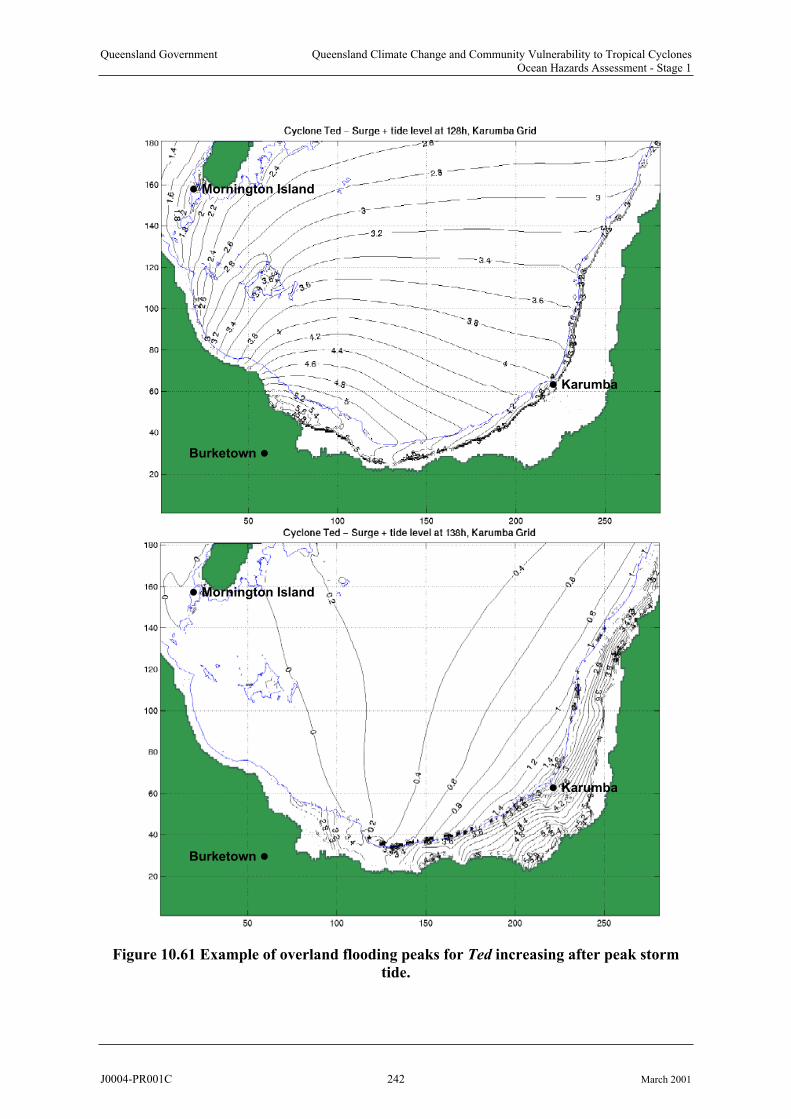
Queensland Government Queensland Climate Change and Community Vulnerability to Tropical CyclonesOcean Hazards Assessment - Stage 1
Karumba
Mornington Island
Burketown
Karumba
Mornington Island
Burketown
Figure 10.61 Example of overland flooding peaks for Ted increasing after peak storm
tide.
J0004-PR001C 242 March 2001
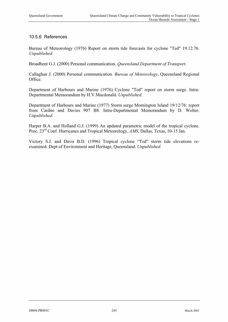
Queensland Government Queensland Climate Change and Community Vulnerability to Tropical CyclonesOcean Hazards Assessment - Stage 1
10.5.6 References
Bureau of Meteorology (1976) Report on storm tide forecasts for cyclone "Ted" 19.12.76. Unpublished.
Broadbent G.J. (2000) Personal communication. Queensland Department of Transport.
Callaghan J. (2000) Personal communication. Bureau of Meteorology, Queensland RegionalOffice.
Department of Harbours and Marine (1976) Cyclone "Ted" report on storm surge. Intra-Departmental Memorandum by H.V.Macdonald. Unpublished.
Department of Harbours and Marine (1977) Storm surge Mornington Island 19/12/76: report from Cardno and Davies 907 B8. Intra-Departmental Memorandum by D. Wolter.Unpublished.
Harper B.A. and Holland G.J. (1999) An updated parametric model of the tropical cyclone. Proc. 23 Conf. Hurricanes and Tropical Meteorology, AMS, Dallas, Texas, 10-15 Jan. rd
Victory S.J. and Davis B.D. (1996) Tropical cyclone “Ted” storm tide elevations re-examined. Dept of Environment and Heritage, Queensland. Unpublished.
J0004-PR001C 243 March 2001

Queensland Government Queensland Climate Change and Community Vulnerability to Tropical CyclonesOcean Hazards Assessment - Stage 1
10.6 Tropical Cyclone Steve February 2000 at Cairns
A synoptic view of the cyclone during the two days prior to landfall is given in Figure 10.62 (after Callaghan 2000). The system became organised and, between 26/1200 UTC and 27/000 UTC, underwent a period of rapid intensification while the centre contracted. The general circulation was highly asymmetric with maximum winds to the SE and, as it moved onshore and intensified, was followed by an E to NE wind surge. The centre tracked between FlindersReef and Willis Island, passed over Holmes Reef and very close to Green Island beforecoming ashore at Yorkeys Knob.
Tropical Cyclone Steve crossed the coast near Yorkeys Knob, 14 km north of Cairns in the early evening of 27th February about 7 pm EST. The cyclone formed from a complex low-pressure system imbedded in a monsoon trough but rapid intensification occurred only as thesystem approached quite close to the coast. Consequently it presented a difficult forecastingproblem and only attained tropical cyclone status and was named barely 12 h before makinglandfall. By landfall it was deemed to have reached Category 2 strength, producing meanwinds of 30 m s-1 at Cairns Airport and caused widespread but generally low level damage to trees and powerlines. It was a very small storm at landfall with an eye diameter of the order of 20 km. As it moved inland it caused major flooding, especially at Mareeba. A storm surge of approximately 1 m was recorded at Cairns Harbour.
Steve continued across Cape York and re-intensified briefly in the Gulf of Carpentaria, thencrossed the Northern Territory and northwestern Western Australia to emerge near Broomeand track down the West Australian coastline as variously a Category 1 or 2 storm. It recurved near Shark Bay and finally lost its circulation on 11th March, south of Esperance in the Great Australian Bight. Steve was notable for its longevity and its significant flooding impactsacross three States. For North Queensland it represented a class of unpredictable mid-intensitycyclones whose storm tide impacts are quite difficult to estimate.
10.6.1 Available Data
Meteorological data for Steve was provided directly by the Severe Weather Section of the Queensland Regional Office of the Bureau of Meteorology. Storm tide information was provided by the Maritime Section of Queensland Transport.
10.6.1.1 Storm Parameters
The official track for this event during the initial period affecting the North Queensland coastwas obtained from the Queensland Regional Office. Wind and pressure data was available from a number of offshore AWS and coastal stations.
The visible satellite image in Figure 10.63 taken a few hours before landfall shows a partly obscured eye in the midst of heavy convection to the east, suggesting the system was still trying to fully organise. The later Cairns radar image at 27/0850 UTC in Figure 10.64 clearly shows the eye, with a diameter of about 22 km, located between Green Island and the coast.
J0004-PR001C 244 March 2001
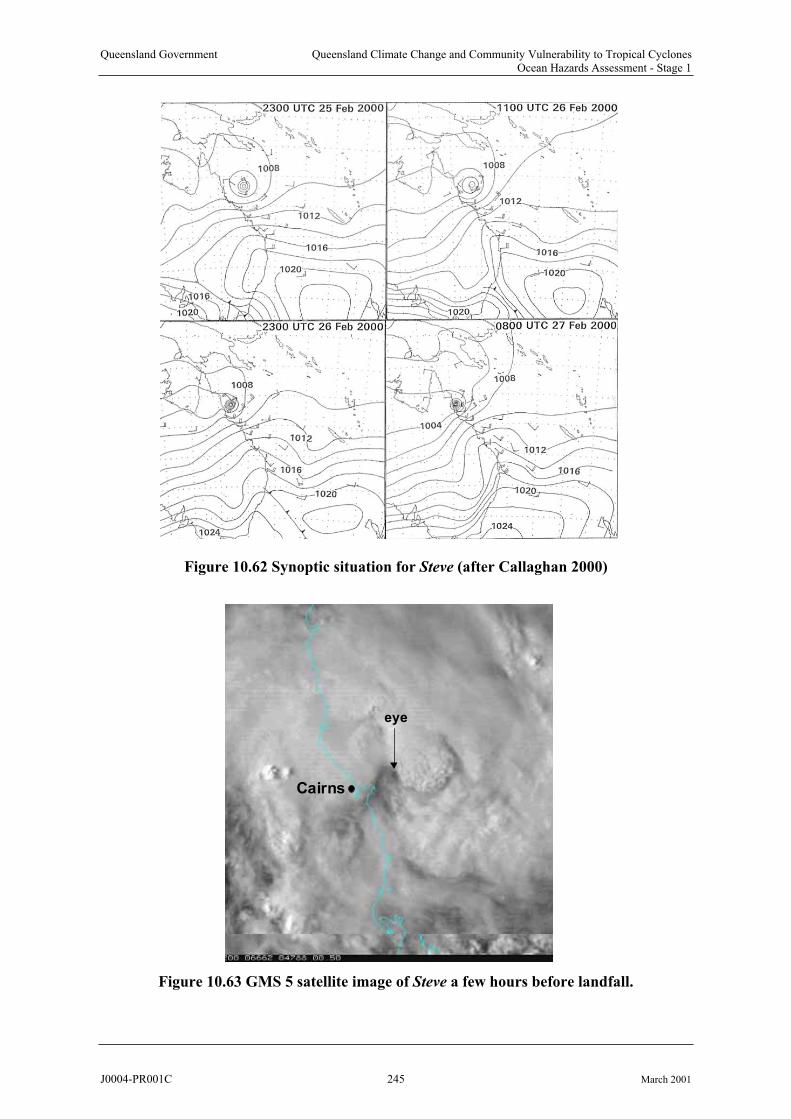
Queensland Government Queensland Climate Change and Community Vulnerability to Tropical CyclonesOcean Hazards Assessment - Stage 1
Figure 10.62 Synoptic situation for Steve (after Callaghan 2000)
Cairns
eye
Figure 10.63 GMS 5 satellite image of Steve a few hours before landfall.
J0004-PR001C 245 March 2001
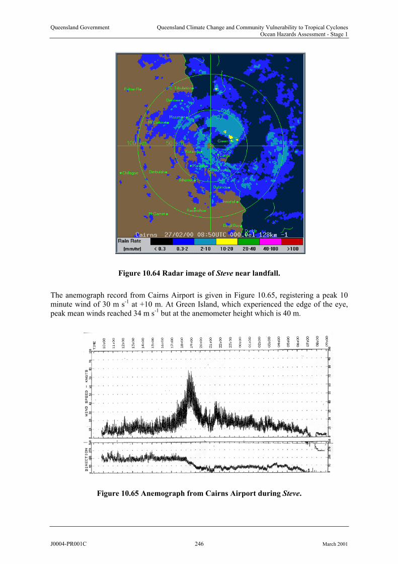
Queensland Government Queensland Climate Change and Community Vulnerability to Tropical CyclonesOcean Hazards Assessment - Stage 1
Figure 10.64 Radar image of Steve near landfall.
The anemograph record from Cairns Airport is given in Figure 10.65, registering a peak 10 minute wind of 30 m s at +10 m. At Green Island, which experienced the edge of the eye, peak mean winds reached 34 m s but at the anemometer height which is 40 m.
-1
Figure 10.65 Anemograph from Cairns Airport during Steve.
-1
J0004-PR001C 246 March 2001
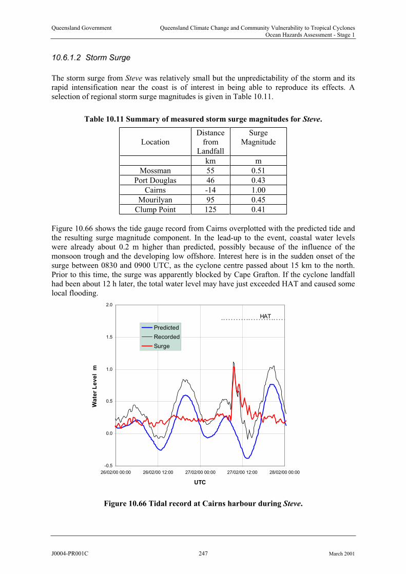
Queensland Government Queensland Climate Change and Community Vulnerability to Tropical CyclonesOcean Hazards Assessment - Stage 1
10.6.1.2 Storm Surge
The storm surge from Steve was relatively small but the unpredictability of the storm and its rapid intensification near the coast is of interest in being able to reproduce its effects. A selection of regional storm surge magnitudes is given in Table 10.11.
Table 10.11 Summary of measured storm surge magnitudes for Steve.
LocationSurge
Magnitude
km m
Mossman 55 0.51
46 0.43
Cairns -14
Mourilyan 95 0.45
125 0.41
Figure 10.66 shows the tide gauge record from Cairns overplotted with the predicted tide andthe resulting surge magnitude component. In the lead-up to the event, coastal water levels were already about 0.2 m higher than predicted, possibly because of the influence of the monsoon trough and the developing low offshore. Interest here is in the sudden onset of the surge between 0830 and 0900 UTC, as the cyclone centre passed about 15 km to the north. Prior to this time, the surge was apparently blocked by Cape Grafton. If the cyclone landfall had been about 12 h later, the total water level may have just exceeded HAT and caused somelocal flooding.
Distancefrom
Landfall
Port Douglas
1.00
Clump Point
-0.5
0.0
0.5
1.0
1.5
2.0
26/02/00 00:00 26/02/00 12:00 27/02/00 00:00 27/02/00 12:00 28/02/00 00:00
UTC
Wa
ter
Le
ve
l m
Predicted
Recorded
Surge
HAT
Figure 10.66 Tidal record at Cairns harbour during Steve.
J0004-PR001C 247 March 2001
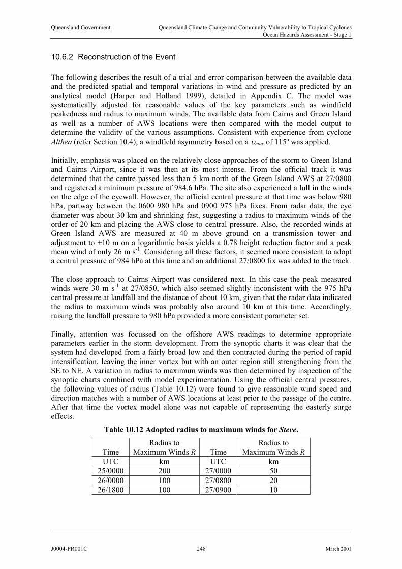
Queensland Government Queensland Climate Change and Community Vulnerability to Tropical CyclonesOcean Hazards Assessment - Stage 1
10.6.2 Reconstruction of the Event
The following describes the result of a trial and error comparison between the available dataand the predicted spatial and temporal variations in wind and pressure as predicted by an analytical model (Harper and Holland 1999), detailed in Appendix C. The model was systematically adjusted for reasonable values of the key parameters such as windfield peakedness and radius to maximum winds. The available data from Cairns and Green Island as well as a number of AWS locations were then compared with the model output todetermine the validity of the various assumptions. Consistent with experience from cyclone
Althea (refer Section 10.4), a windfield asymmetry based on a of 115º was applied. max
Initially, emphasis was placed on the relatively close approaches of the storm to Green Islandand Cairns Airport, since it was then at its most intense. From the official track it was determined that the centre passed less than 5 km north of the Green Island AWS at 27/0800 and registered a minimum pressure of 984.6 hPa. The site also experienced a lull in the winds on the edge of the eyewall. However, the official central pressure at that time was below 980 hPa, partway between the 0600 980 hPa and 0900 975 hPa fixes. From radar data, the eye diameter was about 30 km and shrinking fast, suggesting a radius to maximum winds of the order of 20 km and placing the AWS close to central pressure. Also, the recorded winds at Green Island AWS are measured at 40 m above ground on a transmission tower and adjustment to +10 m on a logarithmic basis yields a 0.78 height reduction factor and a peakmean wind of only 26 m s . Considering all these factors, it seemed more consistent to adopt a central pressure of 984 hPa at this time and an additional 27/0800 fix was added to the track.
-1
The close approach to Cairns Airport was considered next. In this case the peak measuredwinds were 30 m s at 27/0850, which also seemed slightly inconsistent with the 975 hPacentral pressure at landfall and the distance of about 10 km, given that the radar data indicated the radius to maximum winds was probably also around 10 km at this time. Accordingly,raising the landfall pressure to 980 hPa provided a more consistent parameter set.
-1
Finally, attention was focussed on the offshore AWS readings to determine appropriateparameters earlier in the storm development. From the synoptic charts it was clear that the system had developed from a fairly broad low and then contracted during the period of rapid intensification, leaving the inner vortex but with an outer region still strengthening from the SE to NE. A variation in radius to maximum winds was then determined by inspection of thesynoptic charts combined with model experimentation. Using the official central pressures, the following values of radius (Table 10.12) were found to give reasonable wind speed and direction matches with a number of AWS locations at least prior to the passage of the centre.After that time the vortex model alone was not capable of representing the easterly surge effects.
Table 10.12 Adopted radius to maximum winds for Steve.
TimeRadius to
Maximum Winds R TimeRadius to
Maximum Winds R
UTC UTC km
25/0000 200 27/0000 50
26/0000 100 27/0800
26/1800 100 27/0900 10
km
20
J0004-PR001C 248 March 2001
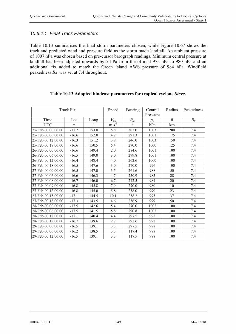
Queensland Government Queensland Climate Change and Community Vulnerability to Tropical CyclonesOcean Hazards Assessment - Stage 1
10.6.2.1 Final Track Parameters
Speed
Table 10.13 summarises the final storm parameters chosen, while Figure 10.67 shows the track and predicted wind and pressure field as the storm made landfall. An ambient pressure of 1007 hPa was chosen based on pre-cursor barograph readings. Minimum central pressure at landfall has been adjusted upwards by 5 hPa from the official 975 hPa to 980 hPa and an additional fix added to match the Green Island AWS pressure of 984 hPa. Windfieldpeakedness B was set at 7.4 throughout. 0
Table 10.13 Adopted hindcast parameters for tropical cyclone Steve.
Track Fix Bearing CentralPressure
Radius Peakedness
Lat Long Vfm fm p0 R B0
UTC m s-1 hPa km
25-Feb-00 00:00:00 153.0 5.8 302.0 1003 200
25-Feb-00 06:00:00 -16.6 152.0 4.2
Time
-17.2 7.4
291.3 1001 175 7.4
25-Feb-00 12:00:00 151.2-16.3 3.8 246.0 1003 150 7.4
25-Feb-00 18:00:00 -16.6 150.5 5.4 270.0 1000 125 7.4
26-Feb-00 00:00:00 -16.6 149.4 2.0 284.6 1001 100 7.4
26-Feb-00 06:00:00 149.0-16.5 3.0 279.8 1001 100 7.4
26-Feb-00 12:00:00 -16.4 100148.4 4.0 262.6 1000 7.4
26-Feb-00 18:00:00 -16.5 147.6 3.0 270.0 996 100 7.4
27-Feb-00 00:00:00 -16.5 147.0 3.5 261.6 988 50 7.4
27-Feb-00 06:00:00 -16.6 146.3 4.7 250.9 985 28 7.4
27-Feb-00 08:00:00 -16.7 146.0 6.7 242.5 984 20 7.4
27-Feb-00 09:00:00 -16.8 145.8 7.9 980270.0 10 7.4
27-Feb-00 12:00:00 145.0-16.8 5.8 238.0 990 23 7.4
27-Feb-00 15:00:00 -17.1 144.5 10.1 258.2 995 37 7.4
27-Feb-00 18:00:00 -17.3 143.5 4.6 256.9 999 50 7.4
28-Feb-00 00:00:00 -17.5 142.6 5.4 270.0 1002 100 7.4
28-Feb-00 06:00:00 -17.5 141.5 5.8 290.8 1002 100 7.4
28-Feb-00 12:00:00 -17.1 140.4 4.4 297.5 995 100 7.4
28-Feb-00 18:00:00 -16.7 139.6 2.7 292.6 992 100 7.4
29-Feb-00 00:00:00 -16.5 139.1 3.3 297.5 988 100 7.4
29-Feb-00 06:00:00 -16.2 3.3 988 7.4138.5 117.4 100
29-Feb-00 12:00:00 139.1 100-16.5 3.3 117.5 988 7.4
J0004-PR001C 249 March 2001
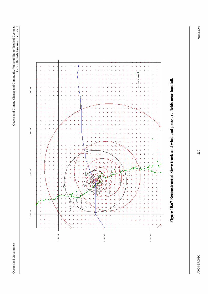
Quee
nsl
and G
over
nm
ent
Qu
een
slan
d C
lim
ate
Ch
ange
and
Co
mm
un
ity
Vuln
erab
ilit
y t
o T
rop
ical
Cy
clo
nes
Oce
an H
azar
ds
Ass
essm
ent
- S
tag
e 1
15
98
59
0
99
5
10
00
10
05
Yo
rk
ey
s
Kn
ob
Po
rt
D
ou
gl
as
Da
in
tr
ee
Go
rd
on
va
le
Ba
bi
nd
a
In
ni
sf
ai
l
Lo
w
Is
le
s
Gr
ee
n
Is
Ho
lm
es
R
ee
f
Ca
ir
ns
A
P
Fl
in
de
rs
R
ee
f
-1
8.
00
-1
7.
00
-1
6.
00
14
5.
00
14
6.
00
14
7.
00
14
8.
00
15
98
59
0
99
5
10
00
10
05
Yo
rk
ey
s
Kn
ob
Po
rt
D
ou
gl
as
Da
in
tr
ee
Go
rd
on
va
le
Ba
bi
nd
a
In
ni
sf
ai
l
Lo
w
Is
le
s
Gr
ee
n
Is
Ho
lm
es
R
ee
f
Ca
ir
ns
A
P
Fl
in
de
rs
R
ee
f
-1
8.
00
-1
7.
00
-1
6.
00
14
5.
00
14
6.
00
14
7.
00
14
8.
00
5
5
5
5
10
10
15
20
25
30
9
5
5
5
5
10
10
15
20
25
30
9
Fig
ure
. R
econ
stru
cted
Ste
ve
track
an
d w
ind
an
d p
ress
ure
fie
lds
nea
r la
nd
fall
.10
67
J0004-P
R001C
250
Mar
ch 2
00
1
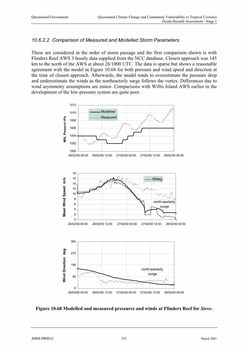
Queensland Government Queensland Climate Change and Community Vulnerability to Tropical CyclonesOcean Hazards Assessment - Stage 1
10.6.2.2 Comparison of Measured and Modelled Storm Parameters
These are considered in the order of storm passage and the first comparison shown is with Flinders Reef AWS 3 hourly data supplied from the NCC database. Closest approach was 145 km to the north of the AWS at about 26/1000 UTC. The data is sparse but shows a reasonable agreement with the model in Figure 10.68 for both pressure and wind speed and direction at the time of closest approach. Afterwards, the model tends to overestimate the pressure drop and underestimate the winds as the northeasterly surge follows the vortex. Differences due to wind asymmetry assumptions are minor. Comparisons with Willis Island AWS earlier in the development of the low-pressure system are quite poor.
Figure 10.68 Modelled and measured pressures and winds at Flinders Reef for Steve.
1000
1002
1004
1006
1008
1010
1012
26/02/00 00:00 26/02/00 12:00 27/02/00 00:00 27/02/00 12:00 28/02/00 00:00
MS
L P
ressu
reh
Pa
Modelled
Measured
0
2
4
6
8
10
12
14
16
18
26/02/00 00:00 26/02/00 12:00 27/02/00 00:00 27/02/00 12:00 28/02/00 00:00
Mean
Win
dS
peed
m/s 65deg
north-easterly
surge
0
90
180
270
360
26/02/00 00:00 26/02/00 12:00 27/02/00 00:00 27/02/00 12:00 28/02/00 00:00
Win
d D
irecti
on
deg
north-easterly
surge
J0004-PR001C 251 March 2001
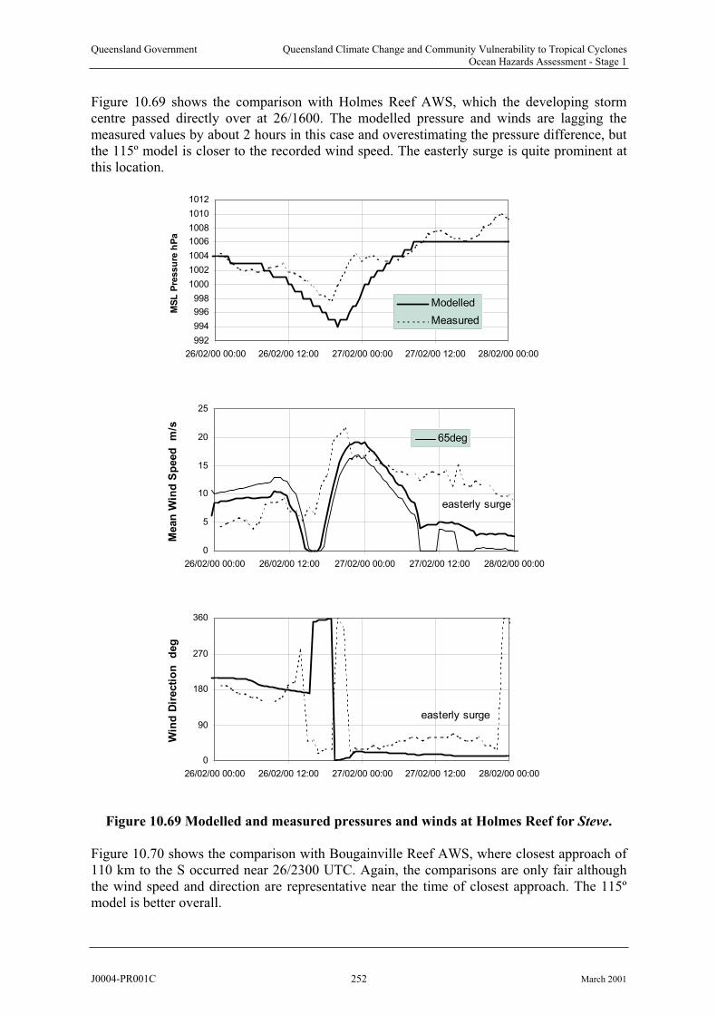
Queensland Government Queensland Climate Change and Community Vulnerability to Tropical CyclonesOcean Hazards Assessment - Stage 1
Figure 10.69 shows the comparison with Holmes Reef AWS, which the developing storm centre passed directly over at 26/1600. The modelled pressure and winds are lagging the measured values by about 2 hours in this case and overestimating the pressure difference, but the 115º model is closer to the recorded wind speed. The easterly surge is quite prominent at this location.
Figure 10.69 Modelled and measured pressures and winds at Holmes Reef for Steve.
992
994
996
998
1000
1002
1004
1006
1008
1010
1012
26/02/00 00:00 26/02/00 12:00 27/02/00 00:00 27/02/00 12:00 28/02/00 00:00
MS
L P
ressu
re h
Pa
Modelled
Measured
0
5
10
15
20
25
26/02/00 00:00 26/02/00 12:00 27/02/00 00:00 27/02/00 12:00 28/02/00 00:00
Mean
Win
d S
peed
m/s
65deg
easterly surge
0
90
180
270
360
26/02/00 00:00 26/02/00 12:00 27/02/00 00:00 27/02/00 12:00 28/02/00 00:00
Win
dD
irecti
on
d
eg
easterly surge
Figure 10.70 shows the comparison with Bougainville Reef AWS, where closest approach of 110 km to the S occurred near 26/2300 UTC. Again, the comparisons are only fair although the wind speed and direction are representative near the time of closest approach. The 115º model is better overall.
J0004-PR001C 252 March 2001
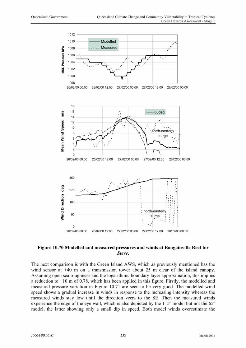
Queensland Government Queensland Climate Change and Community Vulnerability to Tropical CyclonesOcean Hazards Assessment - Stage 1
998
1000
1002
1004
1006
1008
1010
1012
26/02/00 00:00 26/02/00 12:00 27/02/00 00:00 27/02/00 12:00 28/02/00 00:00
MS
L P
ressu
reh
Pa
Modelled
Measured
0
2
4
6
8
10
12
14
16
18
26/02/00 00:00 26/02/00 12:00 27/02/00 00:00 27/02/00 12:00 28/02/00 00:00
Mean
Win
dS
peed
m/s 65deg
north-easterly
surge
0
90
180
270
360
26/02/00 00:00 26/02/00 12:00 27/02/00 00:00 27/02/00 12:00 28/02/00 00:00
Win
dD
irecti
on
d
eg
north-easterly
surge
Figure 10.70 Modelled and measured pressures and winds at Bougainville Reef for
Steve.
The next comparison is with the Green Island AWS, which as previously mentioned has the wind sensor at +40 m on a transmission tower about 25 m clear of the island canopy. Assuming open sea roughness and the logarithmic boundary layer approximation, this impliesa reduction to +10 m of 0.78, which has been applied in this figure. Firstly, the modelled and measured pressure variation in Figure 10.71 are seen to be very good. The modelled wind speed shows a gradual increase in winds in response to the increasing intensity whereas the measured winds stay low until the direction veers to the SE. Then the measured windsexperience the edge of the eye wall, which is also depicted by the 115º model but not the 65ºmodel, the latter showing only a small dip in speed. Both model winds overestimate the
J0004-PR001C 253 March 2001

Queensland Government Queensland Climate Change and Community Vulnerability to Tropical CyclonesOcean Hazards Assessment - Stage 1
measured speed during the storm approach, the 65º case being the worst. It is conjectured thatthe southerly wind at Green Island may actually be shielded by the mainland features such asCape Grafton. After the centre passes, the 115º model better matches the measured wind speeds but neither matches the direction, which remained easterly rather than turning northerly as predicted by the model.
Figure 10.71 Modelled and measured pressures and winds at Green Island for Steve.
980
985
990
995
1000
1005
1010
1015
26/02/00 00:00 26/02/00 12:00 27/02/00 00:00 27/02/00 12:00 28/02/00 00:00
MS
L P
ressu
re h
Pa
Modelled
Measured
0
5
10
15
20
25
30
26/02/00 00:00 26/02/00 12:00 27/02/00 00:00 27/02/00 12:00 28/02/00 00:00
Mean
Win
d S
peed
m
/s
65deg
shielding?
edge of
eye
0
90
180
270
360
26/02/00 00:00 26/02/00 12:00 27/02/00 00:00 27/02/00 12:00 28/02/00 00:00
Win
d D
irecti
on
d
eg
easterly surge
The final comparison is with the Cairns Airport AWS, shown in Figure 10.72. Again, themodelled pressure is very good, together with the peak wind and the change in direction near the peak. Prior to the peak however, the model significantly overestimates the local wind and this is also thought to be due to shielding of the southerly winds by Cape Grafton. As shown
J0004-PR001C 254 March 2001
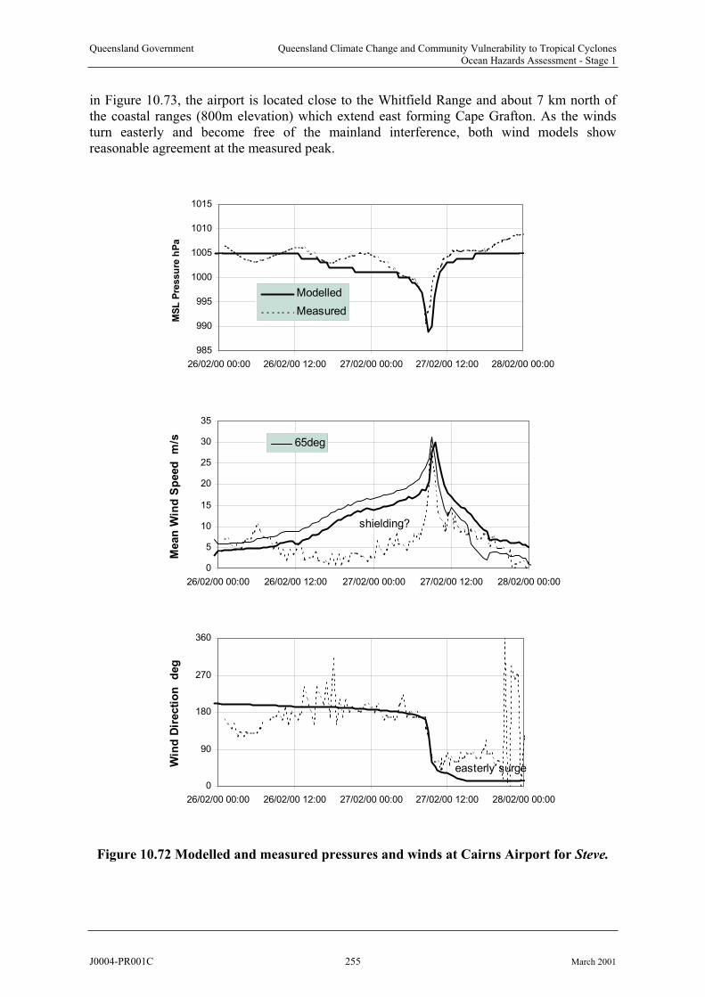
Queensland Government Queensland Climate Change and Community Vulnerability to Tropical CyclonesOcean Hazards Assessment - Stage 1
in Figure 10.73, the airport is located close to the Whitfield Range and about 7 km north of the coastal ranges (800m elevation) which extend east forming Cape Grafton. As the winds turn easterly and become free of the mainland interference, both wind models show reasonable agreement at the measured peak.
Figure 10.72 Modelled and measured pressures and winds at Cairns Airport for Steve.
985
990
995
1000
1005
1010
1015
26/02/00 00:00 26/02/00 12:00 27/02/00 00:00 27/02/00 12:00 28/02/00 00:00
MS
L P
ressu
re h
Pa
Modelled
Measured
0
5
10
15
20
25
30
35
26/02/00 00:00 26/02/00 12:00 27/02/00 00:00 27/02/00 12:00 28/02/00 00:00
Mean
Win
d S
peed
m
/s 65deg
shielding?
0
90
180
270
360
26/02/00 00:00 26/02/00 12:00 27/02/00 00:00 27/02/00 12:00 28/02/00 00:00
Win
d D
irecti
on
d
eg
easterly surge
J0004-PR001C 255 March 2001
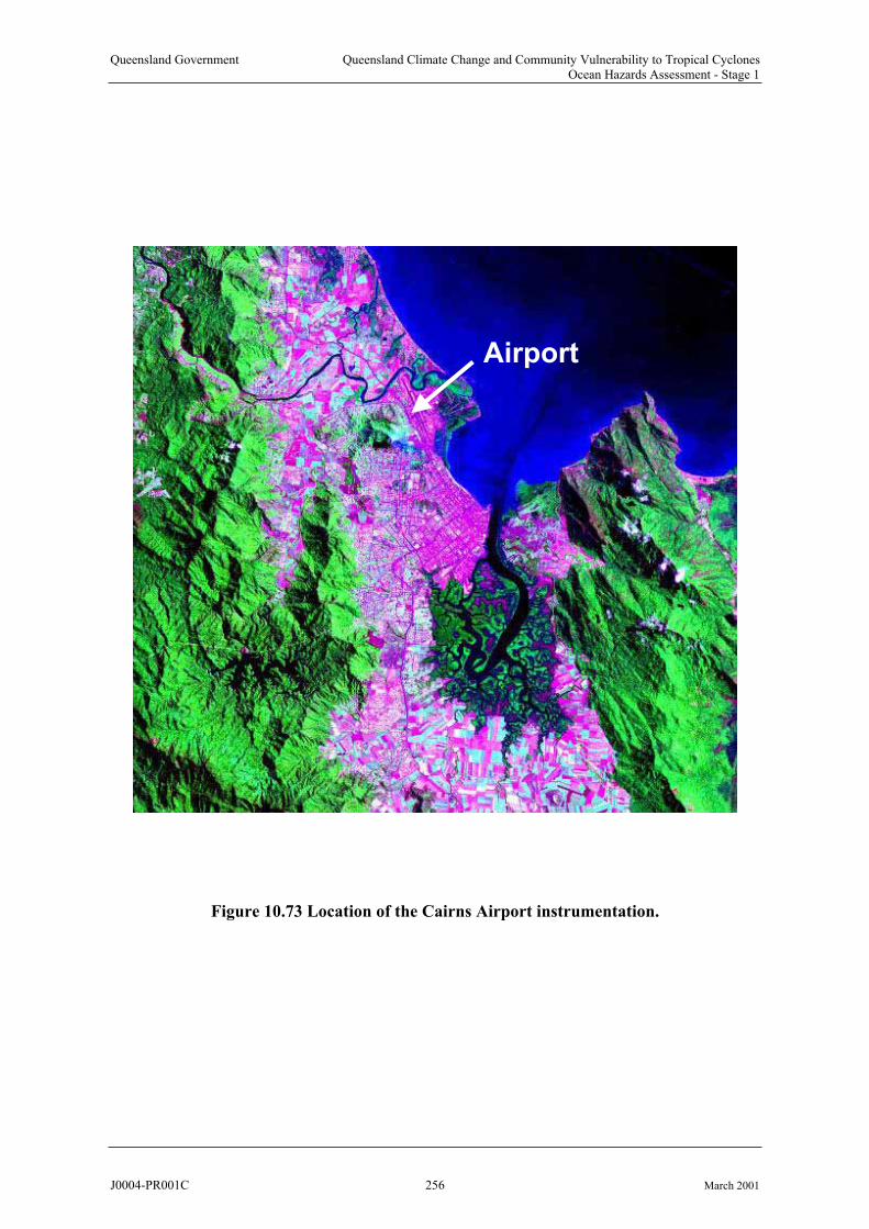
Queensland Government Queensland Climate Change and Community Vulnerability to Tropical CyclonesOcean Hazards Assessment - Stage 1
Airport
Figure 10.73 Location of the Cairns Airport instrumentation.
J0004-PR001C 256 March 2001

Queensland Government Queensland Climate Change and Community Vulnerability to Tropical CyclonesOcean Hazards Assessment - Stage 1
10.6.3 Implications for Storm Surge Modelling
While there remains some difficulty in the model representing the measured wind and pressure data offshore after the centre passes, the model appears adequate for the strongerwinds. In general, the 115º wind model performs better than the 65º although the differences are less compelling than, for example, with Althea, and the present storm was far frommature. The omission of the easterly wind surge effect may affect the broader scale representation of the surge but is not expected to influence the peak value appreciably in thiscase. The overprediction of southerly winds during the approach to Green Island and Cairns is also not likely to cause significant error in the surge calculation since the shielding isessentially a near-coast affect.
In Figure 10.74 below, the modelled envelope of maximum winds shows the band of strong onshore winds which intersect the coast near Cape Grafton and would have acted to produce the small storm tide registered in Cairns Harbour.
20
9 8 5
9 9 0
9 9 0
9 9 5
9 9 5
1 0 0 0
1 0 0 0
P a l m C o v e
Y o r k e y s K n o b
Ma c h a n s B e a c h
C a i r n s
P o r t D o u g l a s
G o r d o n v a l e
G r e e n I s
C a i r n s A P
- 1 7 . 0 0
1 4 6 . 0 0
20
9 8 5
9 9 0
9 9 0
9 9 5
9 9 5
1 0 0 0
1 0 0 0
P a l m C o v e
Y o r k e y s K n o b
Ma c h a n s B e a c h
C a i r n s
P o r t D o u g l a s
G o r d o n v a l e
G r e e n I s
C a i r n s A P
- 1 7 . 0 0
1 4 6 . 0 0
15
2 0
2 5
2 5
3 0
3 015
2 0
2 5
2 5
3 0
3 0
Figure 10.74 Modelled envelope of Steve maximum winds and minimum pressure.
J0004-PR001C 257 March 2001
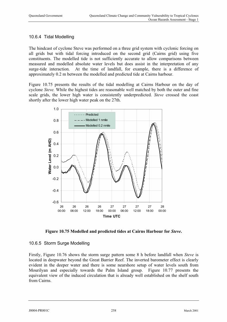
Queensland Government Queensland Climate Change and Community Vulnerability to Tropical CyclonesOcean Hazards Assessment - Stage 1
10.6.4 Tidal Modelling
The hindcast of cyclone Steve was performed on a three grid system with cyclonic forcing onall grids but with tidal forcing introduced on the second grid (Cairns grid) using fiveconstituents. The modelled tide is not sufficiently accurate to allow comparisons between measured and modelled absolute water levels but does assist in the interpretation of any surge-tide interaction. At the time of landfall, for example, there is a difference ofapproximately 0.2 m between the modelled and predicted tide at Cairns harbour.
Figure 10.75 presents the results of the tidal modelling at Cairns Harbour on the day of cyclone Steve. While the highest tides are reasonable well matched by both the outer and fine scale grids, the lower high water is consistently underpredicted. Steve crossed the coastshortly after the lower high water peak on the 27th.
-0.6
-0.4
-0.2
0.0
0.2
0.4
0.6
0.8
1.0
26
00:00
26
06:00
26
12:00
26
18:00
27
00:00
27
06:00
27
12:00
27
18:00
28
00:00
Time UTC
Wate
r L
evel
(m A
HD
)
Predicted
Modelled 1 nmile
Modelled 0.2 nmile
Figure 10.75 Modelled and predicted tides at Cairns Harbour for Steve.
10.6.5 Storm Surge Modelling
Firstly, Figure 10.76 shows the storm surge pattern some 8 h before landfall when Steve islocated in deepwater beyond the Great Barrier Reef. The inverted barometer effect is clearly evident in the deeper water and there is some nearshore setup of water levels south from Mourilyan and especially towards the Palm Island group. Figure 10.77 presents the equivalent view of the induced circulation that is already well established on the shelf south from Cairns.
J0004-PR001C 258 March 2001
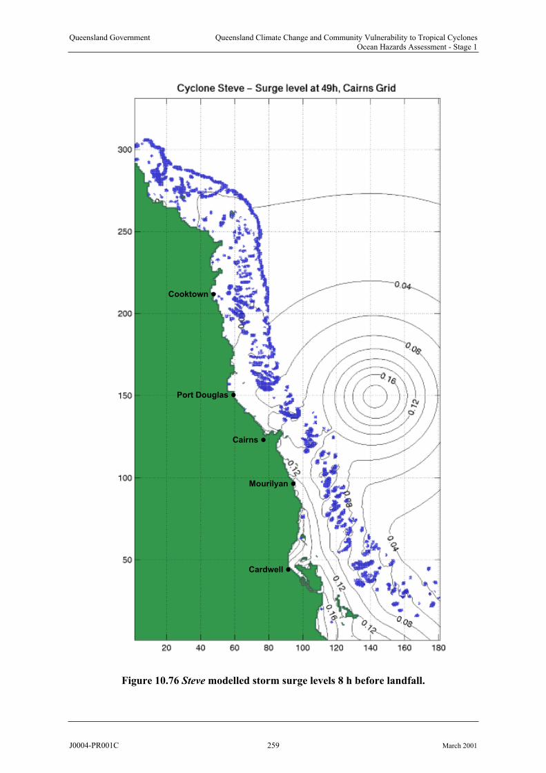
Queensland Government Queensland Climate Change and Community Vulnerability to Tropical CyclonesOcean Hazards Assessment - Stage 1
Cairns
Cardwell
Mourilyan
Port Douglas
Cooktown
Figure 10.76 Steve modelled storm surge levels 8 h before landfall.
J0004-PR001C 259 March 2001

Queensland Government Queensland Climate Change and Community Vulnerability to Tropical CyclonesOcean Hazards Assessment - Stage 1
Cairns
Cardwell
Mourilyan
Port Douglas
Cooktown
J0004-PR001C 260 March 2001
Figure 10.77 Steve modelled storm surge circulation 8 h before landfall.
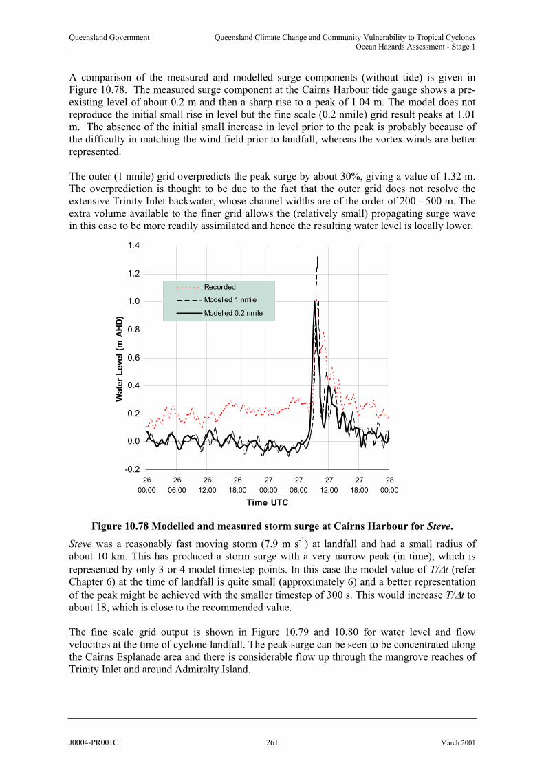
Queensland Government Queensland Climate Change and Community Vulnerability to Tropical CyclonesOcean Hazards Assessment - Stage 1
A comparison of the measured and modelled surge components (without tide) is given in Figure 10.78. The measured surge component at the Cairns Harbour tide gauge shows a pre-existing level of about 0.2 m and then a sharp rise to a peak of 1.04 m. The model does not reproduce the initial small rise in level but the fine scale (0.2 nmile) grid result peaks at 1.01 m. The absence of the initial small increase in level prior to the peak is probably because of the difficulty in matching the wind field prior to landfall, whereas the vortex winds are betterrepresented.
Figure 10.78 Modelled and measured storm surge at Cairns Harbour for Steve.
The fine scale grid output is shown in Figure 10.79 and 10.80 for water level and flow velocities at the time of cyclone landfall. The peak surge can be seen to be concentrated along the Cairns Esplanade area and there is considerable flow up through the mangrove reaches ofTrinity Inlet and around Admiralty Island.
The outer (1 nmile) grid overpredicts the peak surge by about 30%, giving a value of 1.32 m.The overprediction is thought to be due to the fact that the outer grid does not resolve the extensive Trinity Inlet backwater, whose channel widths are of the order of 200 - 500 m. Theextra volume available to the finer grid allows the (relatively small) propagating surge wavein this case to be more readily assimilated and hence the resulting water level is locally lower.
-0.2
0.0
0.2
0.4
0.6
0.8
1.0
1.2
1.4
26
00:00
26
06:00
26
12:00
26
18:00
27
00:00
27
06:00
27
12:00
27
18:00
28
00:00
Time UTC
Wate
r L
evel
(m A
HD
)
Recorded
Modelled 1 nmile
Modelled 0.2 nmile
Steve was a reasonably fast moving storm (7.9 m s-1) at landfall and had a small radius ofabout 10 km. This has produced a storm surge with a very narrow peak (in time), which is
represented by only 3 or 4 model timestep points. In this case the model value of T/ t (refer Chapter 6) at the time of landfall is quite small (approximately 6) and a better representation
of the peak might be achieved with the smaller timestep of 300 s. This would increase T/ t to about 18, which is close to the recommended value.
J0004-PR001C 261 March 2001
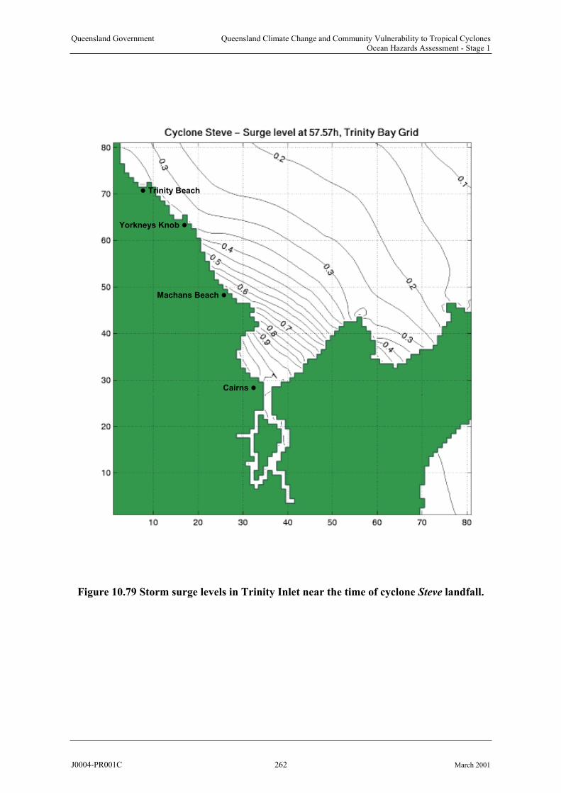
Queensland Government Queensland Climate Change and Community Vulnerability to Tropical CyclonesOcean Hazards Assessment - Stage 1
Cairns
Yorkneys Knob
Machans Beach
Trinity Beach
Figure 10.79 Storm surge levels in Trinity Inlet near the time of cyclone Steve landfall.
J0004-PR001C 262 March 2001

Queensland Government Queensland Climate Change and Community Vulnerability to Tropical CyclonesOcean Hazards Assessment - Stage 1
Cairns
Yorkneys Knob
Machans Beach
Trinity Beach
Figure 10.80 Storm surge velocity in Trinity Inlet near the time of cyclone Steve landfall.
J0004-PR001C 263 March 2001

Queensland Government Queensland Climate Change and Community Vulnerability to Tropical CyclonesOcean Hazards Assessment - Stage 1
Finally, Figure 10.81 shows the comparison between the measured and modelled total water level at Cairns Harbour. The peak surge actually occurred when the predicted tide was very close to MSL and results in a total water level (1.12 m) which is very close to the surge component alone (1.04 m). However, the modelled tide was about 0.2 m lower than predicted at this time such that the fine grid modelled level is lower than measured. Coincidentally, thecoarse grid result, which overpredicted the surge component, is now very close to the measured total water level.
-0.6
-0.4
-0.2
0.0
0.2
0.4
0.6
0.8
1.0
1.2
1.4
26
00:00
26
06:00
26
12:00
26
18:00
27
00:00
27
06:00
27
12:00
27
18:00
28
00:00
Time UTC
Wate
r L
evel
(m A
HD
)
Recorded
Modelled 1 nmile
Modelled 0.2 nmile
Figure 10.81 Measured and modelled total water level at Cairns Harbour during Steve.
10.6.6 References
Broadbent G.J. (2000) Personal communication. Queensland Department of Transport.
Callaghan J. (2000) Personal communication. Bureau of Meteorology, Queensland RegionalOffice.
Harper B.A. and Holland G.J. (1999) An updated parametric model of the tropical cyclone. Proc. 23 Tropical Meteorology, AMS, Dallas, Texas, 10-15 Jan. rd Conf. Hurricanes and
J0004-PR001C 264 March 2001
Queensland Government Queensland Climate Change and Community Vulnerability to Tropical CyclonesOcean Hazards Assessment - Stage 1
10.7 Summary and Conclusions
Four historical tropical cyclones were selected on the basis of their general characteristics,impacts and relevance to forecasting storm tides in Queensland. The paucity of important data for many of these storms has meant that a considerable amount of effort was required to assemble a reasonably accurate reconstruction of each event. The accuracy and coverage of both measured winds and water levels has varied significantly between each storm case, making the process of comparison with modelled winds and water levels somewhat difficult.Also, the degree to which some of the historical water level estimates were affected by wave setup remains unknown.
The hindcast exercise was designed to be as objective as possible; the wind field and water level data were independently assembled by Systems Engineering Australia Pty Ltd and then passed to the James Cook University Marine Modelling Unit for storm surge modelling and comparison. The initial storms tested were Mackay 1918 and Althea and in both cases the initial modelling results indicated that the recorded and/or estimated surge levels would be underpredicted, even though the best possible wind and pressure field data had been assembled. The degree of underprediction varied but was typically of the order of 15% or 0.5 m and prompted a series of sensitivity tests to determine the most likely source of error. Since
existing versions of the storm surge model had utilised rear quadrant maximum winds ( =
115 ), this was one of the tests conducted, and immediately showed a significant improvement in the results for both storms compared with the original front quadrant result
( = 65 ). The modified wind fields were then compared against the anemometer data for Althea and checked for consistency against the sparse Mackay 1918 data. While the Mackay
results remain inconclusive due to a lack of data, the Althea anemometer comparisons are deemed significantly better with the revised rear quadrant winds. Accordingly, the improved storm surge results with the rear quadrant winds are accepted here as the more representativefor those storms. Accordingly, the other storms were similarly modelled, with Ted alsolacking corroborative data but Steve being marginally improved by the rear quadrant wind field. While it is acknowledged that this is a meagre sample from which to draw definiteconclusions, time does not permit a more exhaustive analysis in this context.
max
max
Table 10.14 summarises the results of the four storm validations by comparing peak measuredand modelled storm surge and also storm tide levels at those locations with the most accurate water level data. Shaded parts of the table indicate situations where the best available data is still only an estimate. Considering each storm individually:
Mackay 1918
This has required a significant effort in forensic meteorology, which has achieved admirable success and shows the potential strengths of both parametric wind field models and storm surge models for situations where storms are relatively intense. Theonly normally reliable information on the storm intensity, the Post Office barograph, proved suspect in this case and had to be augmented with a variety of other estimatesand public reports of the passage of the eye and/or turning winds. No measured wind data at all was available. Establishing the maximum water level in the town also required significant research but it is believed that the level of 5.5 m AHD should now be regarded as the definitive impact for this event. Because the level is some distance from the coast and inundation effects were not modelled due to lack of data, there still
J0004-PR001C 265 March 2001

Queensland Government Queensland Climate Change and Community Vulnerability to Tropical CyclonesOcean Hazards Assessment - Stage 1
remains doubt as to the exact open coast storm surge level and the contribution from wave setup. However, the predicted open coast surge plus tide level is only 0.4 m (averaged) below the town level, with the expectation of at least a 0.5 m wave setupcomponent. The timing of the surge also agrees well with eyewitness accounts and the alongshore gradient of surge level is consistent with the reported flooding pattern. The model also indicates non-linear surge and tide interaction plays some part in theMackay region, with a difference of 0.43 m (12%) in the surge component between landfall at MSL compared with the actual high tide levels. The Great Barrier Reef has also been shown to be quite important in this region when modelling combined stormsurge and tide because of its indirect effect in controlling the tidal response. The direct influence on surge magnitude though has been shown to be small.
Table 10.14 Summary of storm surge model hindcast accuracy.
Peak Storm Surge Peak Storm Tide
Measured Modelled Error Measured Modelled Error
Cyclone Ht Time Grid TimeLocation Ht Ht Time Elev Time Elev Time Elev Time
m km m m % mAHD
mAHD
m %
Mackay1918
City 3.50 21:00 1.85 3.38 20:00 -0.12 -3.4 -01:00 5.50 21:00 4.97 20:30 -0.53 -9.6 -00:30
Far Bch 3.72 0.22 6.3 5.28 -0.22 -4.1
1.4(Av.) 3.55 0.05 5.12 -0.38 -6.8
T'ville 2.89 22:40 9.27 3.27 22:45 0.38 13.1 +00:05 2.53 22:40Althea
1.85 2.70 22:45 -0.19 -6.6 +00:05 2.36 22:45 -0.17 -6.9 +00:05
+00:050.37 2.78 22:45 -0.11 -3.8 +00:05 2.44 22:45 -0.09 -3.7
3D 2.96 22:45 0.07 2.4 +00:05
Bowen 0.94 17:00 9.27 0.50 16:30 -0.44 -46.8 -00:30 1.10 17:00
1.85 0.66 17:30 -0.28 -29.8 +00:30 0.95 17:30 -0.15 -13.6 +00:30
Ted Karumba 1.97 11:00 9.27 3.62 08:30 1.65 83.8 -02:30 3.62 09:00 4.36 0.74 20.4 -00:15
0.93 3.31 10:15 1.34 68.0 -00:45 4.00 10:00 0.38 10.5 +01:00
Morning.I.
2.10 03:00 9.27 2.37 03:30 0.27 12.9 +00:30 2.29 03:00 2.16 03:30 -0.13 -5.7 +00:30
0.93 2.85 03:00 0.75 35.7 00:00 2.89 03:15 0.60 26.2 +00:15
Steve Cairns 1.04 09:30 1.85 1.32 09:45 0.28 26.9 +00:15 1.12 09:30 1.20 09:45 0.08 7.1 +00:15
0.37 1.01 09:45 -0.03 -2.9 +00:15 0.89 09:45 -0.23 -20.5 +00:15
Shading indicates estimates only
08:45
Althea
Although Althea has considerably more data, the present study uncovered the need for further assessment of the storm path towards landfall and the effect of the apparent eyewall replacement cycles during that time remains largely unknown. However, the
reconstructed wind and pressure fields (assuming 115 max) are deemed reasonably accurate with peak wind speeds within 3.5% and bias within 5% for the majority ofanemometers available. The resulting storm surge levels are seen to be of comparableaccuracy to the wind speeds, translating to less than 0.2 m error in magnitude of surge and height of storm tide at the Townsville tide gauge. There remains the possibilitythat wave setup and runup contributed significantly to the reported debris levels at other nearby locations. There may also have been higher levels than modelled atlocations closer to the storm track due to the complex eye structure. The Althea testcase has also shown that the Great Barrier Reef has a minor effect on storm surgegeneration in this area and that 3D modelling offers little advantage over 2D.
J0004-PR001C 266 March 2001

Queensland Government Queensland Climate Change and Community Vulnerability to Tropical CyclonesOcean Hazards Assessment - Stage 1
Ted
This storm also presented significant challenges due to the lack of reliable wind and water level data. The track was reconstructed based on a reassessment of all available reports of pressures and winds, although the latter proved unreliable at Mornington Island. The intensity of this storm appears likely to have been greater than official figures prior to its approach to Mornington Island. While the model significantly overpredicted (170%) the surge at the only available recording location of Weipa, theoverall result at Mornington Island and Burketown is consistent with eyewitnessaccounts. The most significant problem in this case is the lack of accurate bathymetryand, because of the low-lying land, the extent of overland flooding which is possible. The present exercise has served to demonstrate the MMUSURGE model's capabilitiesbut falls short of an accurate hindcast due to a lack of detailed data. In addition, the available tidal information for the Gulf is only approximate and hence the actual storm tide levels are not well predicted. Because inundation depends on total water level, and non-linear interactions are likely to be large, it is not possible to improve this result within the present study timeframe.
Steve
While this is a modern event with the benefit of many AWS locations, it is still adifficult storm to characterise and model because of its continuing development during the approach to landfall. Its relatively low intensity has proved the sensitivity of themodel to even small impacts and shown its ability to resolve the complex nearshoreflows on the narrow reef-fringed continental shelf. The focused storm surge at Cairnshas also demonstrated the importance of grid resolution in some situations. Inparticular, the 1.85 km grid overpredicts the storm surge by almost 0.3 m (27%) because it fails to adequately resolve the Trinity Inlet and its storage capacity. For a larger surge, this might not be quite as important since the additional storage will be a smaller proportion of the surge.
Notwithstanding some of the difficulties discussed above, it is concluded that the James Cook University storm surge model MMUSURGE is capable of accurately representing storm surgemagnitudes (<5%) and timing (<15 min) along the Queensland coast, when:
1. The wind and pressure fields can be determined with reasonable certainty, and
2. The bathymetry of the coastal areas is reasonably accurate.
Furthermore, for areas which have well-calibrated tidal boundaries,
3. The model is capable of accurately representing total surge plus tide levels to AHD.
Based on this assessment, and consistent with the recommendations of Chapter 6, it is concluded that accurate nearshore storm tide modelling can be achieved in 2D mode, without non-linear advection, provided that spatial resolutions can correctly resolve the local features (in the range 2 km to 0.5 km) and at timesteps of the order of 900 s (15 min). The Great Barrier Reef parameterisation should be retained to ensure accurate tidal modelling whereverpossible and to maintain correct storm surge magnitude and timing.
J0004-PR001C 267 March 2001

Queensland Government Queensland Climate Change and Community Vulnerability to Tropical CyclonesOcean Hazards Assessment - Stage 1
11. System Design Considerations for Storm Tide Prediction
The study scope requires consideration of the two inter-related approaches to the storm tide problem:
1. Tactical - A storm tide warning capability2. Strategic - A storm tide planning capability
Both capabilities are essential for ensuring minimisation of community impacts from stormtide and each need to be consistently applied and updated with the latest knowledge.Accordingly, there are many aspects of the storm tide problem which are shared by each requirement, namely
Knowledge of cyclone climatology, structure and behaviour
Ability to model wind and pressure fields
Ability to model ocean responses of waves and storm surge
Ability to make predictions in regard to storm tide
Overall accuracy of the prediction
However, needs differ significantly in the following areas:
1. Warnings:
The immediate sensitivity to parameter changes is critical.In essence, the warning problem has no specific requirement to be aware of the statisticallikelihood of any individual storm tide event, except in regard to choosing representative parameter ranges in its various scenario considerations. The accuracy of a prediction for a given set of parameters and the ability to consider uncertainty in those parameter valueswithin a specific time period is the essential requirement. The critical need is for timelyand accurate information for decision making by Government, industry and the generalpublic leading to the minimisation of impact from a specific event.
2. Planning:
The probability of a specific storm tide level is critical.The planning problem, by nature of its extended time scale, needs information for decision making which can be interpreted statistically, leading to an assessment of both relative and absolute levels of risks. Such information can then be used in cost/benefitassessment of planning criteria and for justification of the need for ongoing data collection, research and investigation. The critical need is for a comprehensiveconsideration of the magnitude and frequency of storm tide events which includespotential climatic variability (e.g. inter-decadal) and long term climate change (e.g.Greenhouse). The aim of the planning activity is to minimise the impact from all such events by reducing the community vulnerability in an affordable and practical manner.
Because of these philosophical differences between the warning and planning regimes,differences in the methodologies to achieve their goals also arise. The following sectionsdiscuss these differences and examine opportunities that could be taken to achieve a common outcome of mutual benefit.
J0004-PR001C 268 March 2001
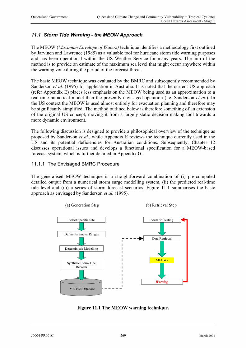
Queensland Government Queensland Climate Change and Community Vulnerability to Tropical CyclonesOcean Hazards Assessment - Stage 1
11.1 Storm Tide Warning - the MEOW Approach
The MEOW (Maximum Envelope of Waters) technique identifies a methodology first outlinedby Jarvinen and Lawrence (1985) as a valuable tool for hurricane storm tide warning purposes and has been operational within the US Weather Service for many years. The aim of the method is to provide an estimate of the maximum sea level that might occur anywhere within the warning zone during the period of the forecast threat.
The basic MEOW technique was evaluated by the BMRC and subsequently recommended by Sanderson et al. (1995) for application in Australia. It is noted that the current US approach (refer Appendix E) places less emphasis on the MEOW being used as an approximation to a real-time numerical model than the presently envisaged operation (i.e. Sanderson et al.). Inthe US context the MEOW is used almost entirely for evacuation planning and therefore maybe significantly simplified. The method outlined below is therefore something of an extension of the original US concept, moving it from a largely static decision making tool towards a more dynamic environment.
The following discussion is designed to provide a philosophical overview of the technique as proposed by Sanderson et al., while Appendix E reviews the technique currently used in theUS and its potential deficiencies for Australian conditions. Subsequently, Chapter 12 discusses operational issues and develops a functional specification for a MEOW-basedforecast system, which is further detailed in Appendix G.
11.1.1 The Envisaged BMRC Procedure
The generalised MEOW technique is a straightforward combination of (i) pre-computeddetailed output from a numerical storm surge modelling system, (ii) the predicted real-timetide level and (iii) a series of storm forecast scenarios. Figure 11.1 summarises the basic approach as envisaged by Sanderson et al. (1995).
(a) Generation Step (b) Retrieval Step
MEOWs
Scenario Testing
Data Retrieval
Define Parameter Ranges
Synthetic Storm TideRecords
Deterministic Modelling
MEOWs Database
Select Specific Site
Warning
Figure 11.1 The MEOW warning technique.
J0004-PR001C 269 March 2001
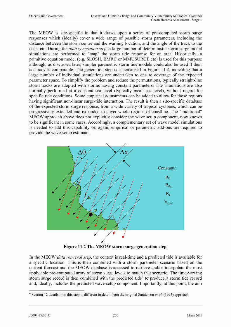
Queensland Government Queensland Climate Change and Community Vulnerability to Tropical CyclonesOcean Hazards Assessment - Stage 1
The MEOW is site-specific in that it draws upon a series of pre-computed storm surge responses which (ideally) cover a wide range of possible storm parameters, including the distance between the storm centre and the warning location, and the angle of the track to the coast etc. During the data generation step, a large number of deterministic storm surge modelsimulations are performed to "map" the storm tide response for an area. Historically, a primitive equation model (e.g. SLOSH, BMRC or MMUSURGE etc) is used for this purpose although, as discussed later, simpler parametric storm tide models could also be used if their accuracy is comparable. The generation step is schematised in Figure 11.2, indicating that a large number of individual simulations are undertaken to ensure coverage of the expectedparameter space. To simplify the problem and reduce the permutations, typically straight-linestorm tracks are adopted with storms having constant parameters. The simulations are alsonormally performed at a constant sea level (typically mean sea level), without regard for specific tide conditions. Some empirical adjustments can be added to allow for those regions having significant non-linear surge-tide interaction. The result is then a site-specific database of the expected storm surge response, from a wide variety of tropical cyclones, which can be progressively extended and expanded to cover whole regions of coastline. The "traditional"MEOW approach above does not explicitly consider the wave setup component, now known to be significant in some cases. Accordingly, a complementary set of wave model simulations is needed to add this capability or, again, empirical or parametric add-ons are required to provide the wave-setup estimate.
Constant:
p0i
B0i
Ri
Vfmi
x
Figure 11.2 The MEOW storm surge generation step.
In the MEOW data retrieval step, the context is real-time and a predicted tide is available fora specific location. This is then combined with a storm parameter scenario based on the current forecast and the MEOW database is accessed to retrieve and/or interpolate the mostapplicable pre-computed array of storm surge levels to match that scenario. The time-varyingstorm surge record is then combined with the predicted tide4 to produce a storm tide record and, ideally, includes the predicted wave-setup component. Importantly, at this point, the aim
4 Section 12 details how this step is different in detail from the original Sanderson et al. (1995) approach.
J0004-PR001C 270 March 2001

Queensland Government Queensland Climate Change and Community Vulnerability to Tropical CyclonesOcean Hazards Assessment - Stage 1
is to provide a maximum envelope of water levels that will incorporate the degree ofuncertainty of the forecast parameters. Therefore, the technique is to generate not one but a variety of potential storm tide outcomes. This is done by a simple perturbation of the forecast parameters on the basis of some type of uncertainty model, which may simply represent the mean and standard deviation, for example, of the historical forecast performance of therelevant storm parameter. The requisite number of scenario results is then extracted from thepre-computed database and the maximum of all the results, together with the forecast timing,becomes the basic warning output from the MEOW technique. Clearly, a statistical description of that envelope can also be provided for specific customer needs.
11.1.2 Conclusions
The MEOW technique appears to satisfy many of the basic requirements for an effective warning system. The approach is simple, easily understood and communicated, and can be adapted over time depending on the operating needs of the forecasting organisation and the community client requirements. Its principal drawback, in traditional form, is the potential need for a large number of simulations during the generation step and the consequent data storage and recovery overheads associated with maintaining the system.
When the method was first devised in the late-1970s, its principal advantage was in overcoming the computational burden of numerical modelling in a real-time context, whereaspresent computer capabilities are significantly greater. However, the basic technique can be directly updated to incorporate either a parametric model data source or a real-time modeldata source without relying on the generation phase and its extensive database. This would be more consistent with the increasing trend towards use of real-time numerical regional weather models, which could provide the boundary conditions of surrounding ambient winds andpressures for the storm surge model vortex and also link directly to track forecasting tools.
11.2 Storm Tide Planning - Statistical Approaches
A variety of methods for attributing probability of exceedance to storm tide levels were reviewed in Chapter 9. The three somewhat similar estimation methods of Monte Carlo
(MCM), Joint Probability (JPM) and Empirical Simulation (EST) were discussed and a recommendation formed which favoured use of either MCM or JPM, depending on the availability of a parametric storm tide model, i.e.
(i) The MCM is generally limited to the use of parametric storm tide models becauseof its many degrees of freedom, which provide advantages for the types of sensitivity testing required in the present project.
(ii) The JPM restricts the range of parameter pairings and assigns probability spaceestimates for later reconstruction, thus permitting increased use of primitive equationmodelling, but without the full freedom of the MCM approach.
The end result in each case, as depicted in Figure 11.3, is a statistical database of storm tide estimates, each built upon a different set of assumptions, yielding long-term probabilities of exceedance of storm tide levels (i.e surge plus tide plus wave setup). The preferred technique is then the one which delivers the greatest accuracy within a practical timeframe and which provides sufficient parameter dynamic range to test sensitivity to factors such as climatechange.
J0004-PR001C 271 March 2001

Queensland Government Queensland Climate Change and Community Vulnerability to Tropical CyclonesOcean Hazards Assessment - Stage 1
Statistical Climatology ofCyclones
Primitive Equation Modelling
Storm Tide Statistics
Synthetic Storm TideRecords
Statistical Database
Parametric Modelling
Monte Carlo Approach Joint Probability Approach
Planning
Figure 11.3 Recommended options for statistical storm tide estimation.
The accuracy of storm tide statistics developed using any of the above methods will benefit greatly from a "seamless" tropical cyclone climatology description of the type discussed in Chapter 9. This should be regarded as an essential pre-requisite for conducting a major stormtide statistics investigation. Such a climatology description will also be valuable for the sensible selection of parameter ranges for any MEOW investigation and can be utilised inreal-time forecasting uncertainty analysis (refer Chapter 12). The climatology descriptionshould include a comprehensive assessment of maximum potential intensity (MPI) as well as inter-seasonal variability (SOI, IPO) and impacts of potential long term climate change (enhanced-Greenhouse).
Implicit in the use of the term "storm tide" is that storm surge, tide and wave setup will beincluded. Wave setup calculations ideally require estimates of local wave heights and periods at resolutions of the order of 500 m, which can only be provided by numerical wave modelling in a manner consistent with that undertaken for storm surge. This will yieldinformation that can be used directly to provide estimates of extreme wave heights and their
J0004-PR001C 272 March 2001

Queensland Government Queensland Climate Change and Community Vulnerability to Tropical CyclonesOcean Hazards Assessment - Stage 1
associated parameters such as period, direction and persistence. The numerical demands of wave modelling are also potentially much greater than that for storm surge alone. If wave action during overland flooding episodes is also to be assessed, nearshore model resolutions will need to be reduced further to the order of 100 m and likely incorporate analytical approximations to wave transformation such as bore formation.
It is clear that the estimation of storm tide statistics for the entire Queensland coast, at an accuracy which will lead to localised or community inundation detail, will require considerable numerical effort. If undertaken in a staged systematic manner, however, this need not be prohibitive and the results will be equally valuable for the storm tide warning
process.
11.3 A Suggested Hybrid Approach
From the above development, it can be seen that there are many shared issues in regard to the desirable capabilities of warning (tactical) and planning (strategic) tools. By combining someof the above concepts a hybrid approach is suggested, which should deliver the relevant accuracy and economies at each stage of the warning and planning processes whilst having a common predictive basis. The overall expected advantage of a combined approach would be to minimise the number of computationally expensive primitive equation model simulations(storm surge and waves) relative to any MEOW and storm tide analyses being undertaken independently.
The suggested key to merging these common aims is to develop parametric models todescribe the regional storm surge and wave response characteristics. In this sense, a parametric (empirical or black box) model is any analytical device that can accuratelydescribe a system response when given a set of parameter inputs. A well-constructed parametric model is one that represents a distillation of otherwise complex knowledge in a concise and efficient framework. The wind and pressure model of Appendix C is an exampleof a very successful parametric model of the complex behaviour of tropical cyclones; the wind stress formulations discussed in Chapter 6 are likewise simple parametric models. In thepresent context, parametric models of storm surge and waves would be constructed based on
the results of a series of primitive equation storm surge and spectral wave model results.
As discussed in Chapter 9, simple parametric storm tide models (storm + tide only) havealready been used extensively in establishing storm tide statistics for the Queensland coast, e.g. Harper and McMonagle (1985). Their apparent utility, even based on limited underlying numerical modelling, is due to the largely linear relationship between storm intensity and peak surge height at many coastal locations. This results in a similarity behaviour that allowsscaling of the surge response. Harper (1983) extended this concept to include extreme waves and wave setup by combining with limited spectral wave modelling and the results comparefavourably with recent statistical analyses of long-term wave data (M. Allen, EPA, pers.
comm.). Recently updated analyses of the storm tide risk at the Gold coast (GCCC 1999) arealso very similar to values developed initially by Harper and McMonagle (1985). Examples of the application of this circa 1985 parametric model to Althea and the 1918 Mackay cyclone are given in Figures 11.4 and 11.5 respectively, derived from studies described in Harper (1996) and labelled here as MIRAM. This simple model is based on interpolation of numerical model results between only three storm intensities at each of three approachdirections, with a forward speed adjustment factor based on Nickerson
J0004-PR001C 273 March 2001

Queensland Government Queensland Climate Change and Community Vulnerability to Tropical CyclonesOcean Hazards Assessment - Stage 1
-1.0
-0.5
0.0
0.5
1.0
1.5
2.0
2.5
3.0
23
00:00
23
06:00
23
12:00
23
18:00
24
00:00
24
06:00
24
12:00
24
18:00
25
00:00
Time UTC
Wate
r L
evel
(m
AH
D)
MIRAM
JCU
Recorded
Figure 11.4 MIRAM parametric storm tide model prediction for Althea.
-2
-1
0
1
2
3
4
5
6
20
14:00
20
15:00
20
16:00
20
17:00
20
18:00
20
19:00
20
20:00
20
21:00
20
22:00
20
23:00
21
00:00
21
01:00
Time UTC
Wate
r L
evel
(m A
HD
)
JCU + Tide
JCU No Tide
MIRAM
MIRAM + Setup
Measured
Figure 11.5 MIRAM parametric model prediction for the 1918 Mackay.
J0004-PR001C 274 March 2001

Queensland Government Queensland Climate Change and Community Vulnerability to Tropical CyclonesOcean Hazards Assessment - Stage 1
(1971) and a constant B and R. The model also incorporates a basic wave setup predictorwhich is proportional to storm central pressure. Hence, a simple parametric model based on only nine numerical simulations is capable of producing a storm tide estimate of notionally similar accuracy to the present primitive equation result for these two storms.
It is argued that a more sophisticated parametric model could now be developed with the advantages of improved and more efficient primitive equation models. For example, the spatial resolution of the original numerical modelling was limited to 5 n mile (9.25 km). The above parametric model is presently limited to prediction of coastal storm tide levels only but can simultaneously represent a number of coastal locations with varying tidal characteristicsand local storm surge and wave height amplification factors. Importantly, the model provides the estimated time history of water levels for phase interaction with the tide. If a velocity fieldis required or a full spatial description of the water level field is needed, a primitive equationmodel result is essential. Given that the parametric model must be developed from a set of primitive equation model simulations, such detailed datasets will remain available forsubsequent application in any allied areas.
Taking all of the above into consideration, Figure 11.6 provides an overview of a possible way forward, consisting of three basic elements:
1. The first element relates to establishment of a comprehensive statisticalclimatology of tropical cyclones. Next follows the large scale deterministicmodelling of discrete parameter selections from that climatology using primitiveequation models for surge and waves. These results would form an extensivesynthetic storm tide (surge and wave) database for specific regions. Based on that database, a series of regional parametric storm tide models would then bedeveloped. The parametric models will then be applied in association with the statistical aspects of the climatology to generate synthetic storm tide records,leading directly to the establishment of storm tide statistics for planning
purposes.
2. Under the second element, the same parametric (surge and wave) models would be used within the Bureau AIFS forecasting environment as a simple MEOWpreparedness tool, designed for rapid real-time scenario testing having a high availability and a low likelihood of failure. The climatology would be used forforecast uncertainty analysis.
3. The third element would interface the deterministic storm surge and wavemodels used previously to the Bureau TCLAPS atmospheric model and associated tropical cyclone track forecasting tools. The numerical surge and wave models would then make use of the best wind and pressure information in an integrated environment and could incorporate tidal modelling, thus avoiding the surge-tide interaction issue in the warning context. A limited set of MEOWscenarios would then be undertaken in real-time, again guided by the established climatology. While this approach is already technically feasible (refer Table 11.3 later), it will become more so in the coming years as computer memory andcomputational speeds continue to increase.
This hybrid approach has the capacity to integrate both warning and planning needs in a consistent and mutually beneficial staged development. The parametric models could be
J0004-PR001C 275 March 2001
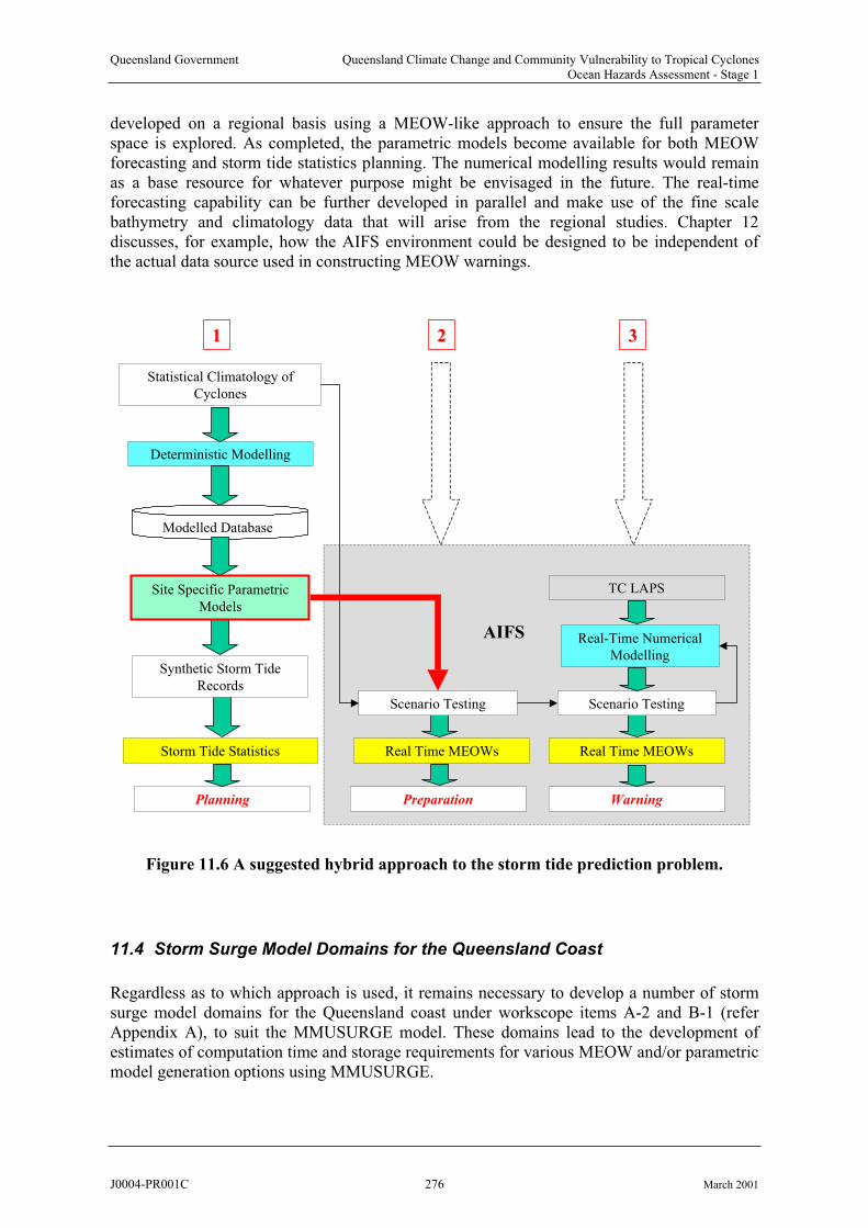
Queensland Government Queensland Climate Change and Community Vulnerability to Tropical CyclonesOcean Hazards Assessment - Stage 1
developed on a regional basis using a MEOW-like approach to ensure the full parameterspace is explored. As completed, the parametric models become available for both MEOWforecasting and storm tide statistics planning. The numerical modelling results would remainas a base resource for whatever purpose might be envisaged in the future. The real-timeforecasting capability can be further developed in parallel and make use of the fine scalebathymetry and climatology data that will arise from the regional studies. Chapter 12 discusses, for example, how the AIFS environment could be designed to be independent of the actual data source used in constructing MEOW warnings.
AIFS
Statistical Climatology of
Cyclones
Deterministic Modelling
Real Time MEOWsStorm Tide Statistics
Synthetic Storm Tide
Records
Modelled Database
Site Specific Parametric
Models
Real Time MEOWs
TC LAPS
Real-Time Numerical
Modelling
Scenario Testing Scenario Testing
2
WarningPlanning
1
Preparation
31 2 3
Figure 11.6 A suggested hybrid approach to the storm tide prediction problem.
11.4 Storm Surge Model Domains for the Queensland Coast
Regardless as to which approach is used, it remains necessary to develop a number of stormsurge model domains for the Queensland coast under workscope items A-2 and B-1 (refer Appendix A), to suit the MMUSURGE model. These domains lead to the development of estimates of computation time and storage requirements for various MEOW and/or parametricmodel generation options using MMUSURGE.
J0004-PR001C 276 March 2001
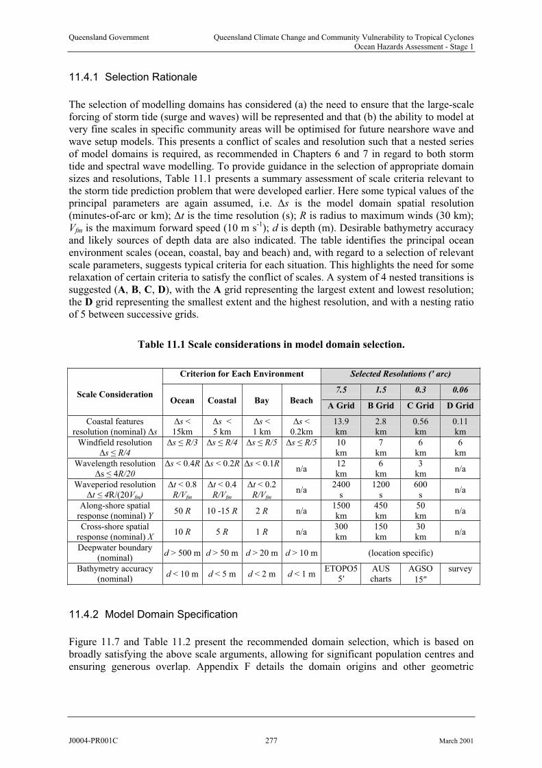
Queensland Government Queensland Climate Change and Community Vulnerability to Tropical CyclonesOcean Hazards Assessment - Stage 1
11.4.1 Selection Rationale
The selection of modelling domains has considered (a) the need to ensure that the large-scaleforcing of storm tide (surge and waves) will be represented and that (b) the ability to model at very fine scales in specific community areas will be optimised for future nearshore wave and wave setup models. This presents a conflict of scales and resolution such that a nested seriesof model domains is required, as recommended in Chapters 6 and 7 in regard to both storm tide and spectral wave modelling. To provide guidance in the selection of appropriate domainsizes and resolutions, Table 11.1 presents a summary assessment of scale criteria relevant tothe storm tide prediction problem that were developed earlier. Here some typical values of the principal parameters are again assumed, i.e. s is the model domain spatial resolution(minutes-of-arc or km); t is the time resolution (s); R is radius to maximum winds (30 km);Vfm is the maximum forward speed (10 m s-1); d is depth (m). Desirable bathymetry accuracyand likely sources of depth data are also indicated. The table identifies the principal oceanenvironment scales (ocean, coastal, bay and beach) and, with regard to a selection of relevant scale parameters, suggests typical criteria for each situation. This highlights the need for somerelaxation of certain criteria to satisfy the conflict of scales. A system of 4 nested transitions is suggested (A, B, C, D), with the A grid representing the largest extent and lowest resolution;the D grid representing the smallest extent and the highest resolution, and with a nesting ratioof 5 between successive grids.
Table 11.1 Scale considerations in model domain selection.
Criterion for Each Environment Selected Resolutions ( arc)
7.5 1.5 0.3 0.06Scale Consideration
Ocean Coastal Bay BeachA Grid B Grid C Grid D Grid
Coastal featuresresolution (nominal) s
s < 15km
s <5 km
s <1 km
s < 0.2km
13.9km
2.8km
0.56km
0.11km
Windfield resolutions R/4
s R/3 s R/4 s R/5 s R/5 10km
7km
6km
6km
Wavelength resolutions 4R/20
s < 0.4R s < 0.2R s < 0.1Rn/a
12km
6km
3km
n/a
Waveperiod resolutiont 4R/(20Vfm)
t < 0.8R/Vfm
t < 0.4R/Vfm
t < 0.2R/Vfm
n/a2400
s1200
s600
sn/a
Along-shore spatial response (nominal) Y
50 R 10 -15 R 2 R n/a1500km
450km
50km
n/a
Cross-shore spatialresponse (nominal) X
10 R 5 R 1 R n/a300km
150km
30km
n/a
Deepwater boundary(nominal)
d > 500 m d > 50 m d > 20 m d > 10 m (location specific)
Bathymetry accuracy (nominal)
d < 10 m d < 5 m d < 2 m d < 1 mETOPO5
5AUScharts
AGSO
15
survey
11.4.2 Model Domain Specification
Figure 11.7 and Table 11.2 present the recommended domain selection, which is based on broadly satisfying the above scale arguments, allowing for significant population centres and ensuring generous overlap. Appendix F details the domain origins and other geometric
J0004-PR001C 277 March 2001

Queensland Government Queensland Climate Change and Community Vulnerability to Tropical CyclonesOcean Hazards Assessment - Stage 1
properties needed to specify their properties to the model's spherical coordinate system (described in Appendix D).
Only A and B domains are defined here because of the readily available bathymetry set,which is limited to ETOPO5 (5 arc) in deep water, augmented by the AUS hydrographic
chart and bathymetric series in shelf and nearshore regions. AGSO 30 data was also considered in this regard but in discussions with AGSO personnel it was not considered greatly superior to the data already available to the Marine Modelling Unit derived from the
other sources. Higher resolution data (e.g. AGSO's planned 15 arc dataset) would be required for C grids5, while D grids would demand local survey data. It is considered that such fine scale grids need to be developed in the context of undertaking detailed regional studies. Whileparts of the grid generation can be automated, there remains a significant amount of manualintervention required to ensure the grid depths are commensurably accurate with the spatial resolution and that the actual coastline is properly preserved. The availability of some C grid data domains for Townsville and Cairns, which were used for the present hindcast activity, isdue to earlier research studies conducted by the Marine Modelling Unit. That data would be available to assist in compatible C and/or D grid construction for those regions.
Table 11.2 Selected MEOW model domain parameters.
Timestep Resolution Extent Dimension (km)GridNo. Location
s ' arc km Alongshore Offshore Alongshore Offshore
A0 Queensland Coast 1800 7.5 13.9 201 57 2780 778
A1 SouthernQueensland
1800 7.5 13.9 101 57 1390 778
A2 Central Queensland 1800 7.5 13.9 101 57 1390 778
A3 NorthernQueensland
1800 7.5 13.9 101 57 1390 778
A4 Gulf of Carpentaria 1800 7.5 13.9 105 117 1966 1612
B1 Brisbane 900 1.5 2.8 161 65 448 179
B2 Hervey Bay - Gladstone
900 1.5 2.8 153 61 426 168
B3 Mackay 900 1.5 2.8 161 125 448 347
B4 Whitsunday 900 1.5 2.8 201 101 560 280
B5 Townsville 900 1.5 2.8 161 65 448 179
B6 Cairns 493900 1.5 2.8 177 45 123
B7 Cooktown 900 1.5 2.8 161 73 448 202
B8 Lockhart River 414900 1.5 2.8 149 65 179
B9 Torres Strait 900 1.5 2.8 131 141 364 392
B10 Weipa 2.8 112900 1.5 161 41 448
Karumba 1.5 169 470 134
Mornington Island 1.5 161 448 157
B11 900 2.8 49
B12 900 2.8 57
5 Testing of Althea using the recommended A2 and B5 grids here shows only a 3% overprediction relative to therecorded water levels as detailed in Section 10.
J0004-PR001C 278 March 2001
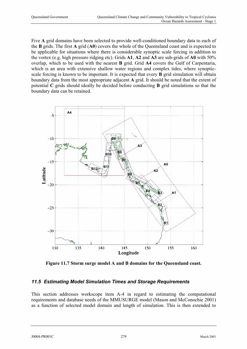
Queensland Government Queensland Climate Change and Community Vulnerability to Tropical CyclonesOcean Hazards Assessment - Stage 1
Five A grid domains have been selected to provide well-conditioned boundary data to each of the B grids. The first A grid (A0) covers the whole of the Queensland coast and is expected tobe applicable for situations where there is considerable synoptic scale forcing in addition tothe vortex (e.g. high pressure ridging etc). Grids A1, A2 and A3 are sub-grids of A0 with 50%overlap, which to be used with the nearest B grid. Grid A4 covers the Gulf of Carpentaria,which is an area with extensive shallow water regions and complex tides, where synoptic-scale forcing is known to be important. It is expected that every B grid simulation will obtain boundary data from the most appropriate adjacent A grid. It should be noted that the extent of potential C grids should ideally be decided before conducting B grid simulations so that theboundary data can be retained.
B1
B2
B3B4
B5
B6
B7
B10B8
B11B12
B9
A4
A3
A2
A1
A0
Figure 11.7 Storm surge model A and B domains for the Queensland coast.
11.5 Estimating Model Simulation Times and Storage Requirements
This section addresses workscope item A-4 in regard to estimating the computational requirements and database needs of the MMUSURGE model (Mason and McConochie 2001) as a function of selected model domain and length of simulation. This is then extended to
J0004-PR001C 279 March 2001

Queensland Government Queensland Climate Change and Community Vulnerability to Tropical CyclonesOcean Hazards Assessment - Stage 1
consider the implementation of some specific MEOW data generation steps utilising Bureau of Meteorology computing resources within the Queensland Regional Office.
11.5.1 Model Requirements
The MMUSURGE storm surge model is implemented in FORTRAN 90 and its computationalspeed is somewhat dependent on the specific architecture of the machine being used (instruction set, caching, pipelining etc) in addition to the base CPU clock speed. Its memoryrequirements may also be slightly non-linear relative to domain size because of the implicitmatrix solution of the hydrodynamic equations. It is also likely to be sensitive to the operating system being used (e.g. UNIX™, LINUX™ or Windows™ NT/2000). The model has been developed and run successfully to date on a variety of UNIX™-based machines at JamesCook University.
Under Part B-1 of the current workscope MMUSURGE has been ported to the CIRRUS1workstation at the Queensland Regional Office of the Bureau of Meteorology in Brisbane, which has the following configuration:
2 x 9.1GB disk
XLF90 FORTRAN 90
IBM 43P Model 150 PowerPC™ 604e 375MHz 512 MB RAM
AIX™ 4.3.3 operating system ( a UNIX™ variant)6
Benchmark testing has shown that the above machine7 has comparable performance to any Intel™ Celeron™ level personal computer of similar clock speed and that only modest RAM (e.g. 64 MB) and disk storage (e.g. 1 GB) is needed to successfully execute the MMUSURGEmodel. Based on discussions with Queensland Regional Office computing staff, a number of machines of this capacity could be utilised wholly or partly within Regional Office. It mayeven be possible to install joint operating systems (LINUX™/Windows™) on machines that are only lightly loaded, without inconveniencing normal operations. Data archiving requirements will need to be separately addressed.
Assuming CIRRUS1 is utilised, Table 11.3 presents actual CPU time (min) and disk storage(MB) required as a function of storm duration for each of the A and B grids. The disk storagecalculation assumes all model output parameters (H,U,V) at all grid points are output in binary at every timestep (e.g. 30 min for A grid; 15 min for B grid), together with 10 timehistory locations. Allowance is also made for the A-B grid boundary transition file. Note that each B grid simulation must have a corresponding A grid simulation as well and the totalunder "Option (i)" in Table 11.3 allows for this fact. For example, to process a single 24 h storm scenario in each of the 12 B grid domains would require 105 h CPU time and generate206 MB of disk output on CIRRUS1.
Table 11.3 "Option (i)" represents the "base case" whereby the full model capability is utilisedand full output is retained. To reduce computational overheads for open coast MEOWs it is
6 An ANSI compliant FORTRAN 90 compiler is required to generate an executable version of the model andMATLAB™ is required to access the graphical output capabilities.7 Latest Compaq Alpha™, Intel Pentium III™ and AMD Athlon™ processors would likely exceed thecomputational speed of CIRRUS1 by a factor of 2 or 3 or more.
J0004-PR001C 280 March 2001

Queensland Government Queensland Climate Change and Community Vulnerability to Tropical CyclonesOcean Hazards Assessment - Stage 1
recommended that the non-linear advection terms in the model momentum calculation beomitted. Their contribution to water levels is shown to be generally small (refer Section 10.7) and a saving of approximately 15% in simulation time is obtained as indicated by "Option (ii)". This recommendation is also consistent with that by Sanderson et al. (1995) in regard to the present BMRC model. In addition, as shown in "Scenario (iii) and (iv)" the output data may be drastically reduced if it is deemed necessary only to retain information either a shortdistance out to sea or just along the coast. Caution is advised however in limiting the data tooseverely given the high CPU cost in conducting the simulations and the potential value of full field data for other future purposes. Note that time and disk estimates for each "Option" in Table 11.3 are additive.
Based on the above domain-specific CPU and storage parameters it is possible to estimate the order-of-magnitude computational effort to undertake a range of MEOW modelling studiesfor the whole of the Queensland coast. "Option (iii)" with a 24 h storm duration is retained forfurther consideration in the analysis of Table 11.4.
Table 11.3 CPU and disk storage requirements for MMUSURGE on the CIRRUS1
workstation.
CPU Minutes for Duration Disk Storage MB for DurationGridNo. Location
24 h 48 h 72 h 96 h 24 h 48 h 72 h 96 h
Southern Queensland 3.0 4.5 6.0 3.3 6.5 9.8 13.0
A2 Central Queensland 3.81.9 5.6 7.5 3.3 6.5 9.8 13.0
A3 Northern Queensland 1.8 3.6 5.5 7.3 3.3 6.5 9.8 13.0
A4 Gulf of Carpentaria 9.0 11.7 23.42.2 4.5 6.7 5.8 17.5
B1 Brisbane 3.7 7.3 11.0 14.7 11.3 22.7 34.0 45.3
B2 Hervey Bay -Gladstone
3.5 7.0 20.510.4 13.9 10.3 30.8 41.1
Mackay 13.9 27.8 55.6 22.1 44.2 66.4 88.5
B4 Whitsunday 13.7 27.5 41.2 55.0 22.3 44.6 66.9 89.3
Townsville 6.7 13.4 20.1 26.8 11.5 23.0 34.5 46.0
B6 Cairns 5.9 11.7 17.6 23.4 8.8 17.5 26.3 35.0
B7 Cooktown 8.0 16.0 24.1 32.1 12.9 25.8 38.8 51.7
B8 Lockhart River 8.2 16.3 24.5 32.7 10.7 21.3 32.0 42.6
B9 Torres Strait 12.3 24.6 36.9 49.2 20.3 40.6 60.9 81.2
B10 Weipa 1.7 3.4 5.2 6.9 7.3 14.5 21.8 29.1
B11 Karumba 2.1 4.2 6.4 8.5 9.1 18.2 27.3 36.4
B12 Mornington Island 2.4 4.7 7.1 9.4 10.1 20.2 30.3 40.4
(i) All grids (per storm) 105 210 315 419 206 412 618 824
(ii) Advection 0 89 178 267 356 206 412 618 824
(iii) Within 10 points of the
coast
210 315 419 16.2 48.6 64.8
(iv) Coast data only 105 210 315 419 1.6 3.2 4.9 6.5
A1 1.5
B3 41.7
B5
Possible Options
32.4105
J0004-PR001C 281 March 2001

Queensland Government Queensland Climate Change and Community Vulnerability to Tropical CyclonesOcean Hazards Assessment - Stage 1
11.5.2 MEOW Parameter Selection
1. "Ideal"
The number of MEOW storm simulations required is controlled by permutations of thenumber of point values selected to span the desirable range of model storm parameters. For illustration and discussion purposes, a number of scenarios are presented below and
summarised in Table 11.4. The parameter ranges considered are { p , B , R , Vfm , fm , X ,
max } and each is specified in terms of a nominal start or lower bound, an interval, and an end or upper bound. The total number of simulations required to cover each parameter range is then indicated and the total permutations calculated, together with the estimated CPU time(weeks on CIRRUS1) and disk storage (GB assuming all data is retained). In each case it isassumed that "Option (iii)" from Table 11.3 is adopted, together with a storm duration of 24 h.Figure 11.8 summarises the resulting CPU and disk storage relationships graphically for eachscenario.
The five scenarios presented here are:
This is a simple discretisation of the tropical cyclone parameter space based on "ideal" scales of variation i.e. linearly spaced intervals covering the expected range at a nominalresolution. Only half the full along-shore grid extent is used here due to overlap. Whilst these chosen parameter ranges and resolutions are familiar in terms of known storm surge sensitivities, it is clear that such a MEOW selection is not practically achievable,probably even with supercomputer capability.
2. "Desirable"
Scenario 2 below assumes a coarser X resolution and a limited coverage of each MEOWgrid, with nominal reductions in all the other parameters. In this case, the coastalcrossings would be concentrated only at significant population areas. Further discussion on Scenario 2 is included later.
3. Current US practice
This is based on the information provided in FEMA et al. (1999), as discussed in detail in Appendix E. This scenario is characterised by well defined directions and closely spacedtracks (which are varied according to direction etc) but considers only a single value for Rand B. The target region considered is the northwest Gulf of Mexico.
4. BoM QRO
This refers to BoM (1999), a preliminary MEOW exercise conducted in Queensland Regional Office. This scenario has reduced directional and intensity resolution comparedwith the US practice but allows for variation in R. The target regions envisaged were Cairns, Townsville and Mackay.
J0004-PR001C 282 March 2001

Queensland Government Queensland Climate Change and Community Vulnerability to Tropical CyclonesOcean Hazards Assessment - Stage 1
It should be noted that only scenarios 1 and 2 here consider variation in B, which has been shown even within the present hindcast modelling to be an important storm surge parameter.
5. BMRC
Refers to Sanderson et al. (1995), the BMRC review and recommendation report on implementing MEOW techniques in the Australian context. This has the coarsestdirectional and X resolution and was nominally considered to apply to the Mackay region.
Table 11.4 Estimated run times and storage needs for example MEOW scenarios.
"Option (iii)" and 24 h Duration
Scenario 1 Scenario 2 Scenario 3 Scenario 4 Scenario 5
Storm "ideal" "desirable" US Practice BoM QRO BMRC
Unit Range Values Totals Values Totals Values Totals Values Totals Values Totals
Start 10 10 15 15 35
p hPa Interval 10 11 420 6 20 5 25 4 25
End 110 110110 95 90
Start 1 1 1 1.5 1.5
B Interval 0.25 7 0.5 3 0 1 0 1 0 1
End 2.5 2 1 1.5 1.5
Start 5 10 40 10 10
R km Interval 10 6 25 3 0 1 25 3 25 3
End 55 60 40 60 60
Start 2.5 2 2.2 0 0
Vfm m s-1 Interval 2.5 5 2 4 4.5 3 5 4 5 4
End 12.5 8 11.2 15 15
Start 0 0 0 0 0
fmº Interval 11.25 17 22.5 9 11.25 17 30 5 45 4
End 180 180 180 120 135
Start 0 -100 -100 -500 -300
km Interval 20 11 25 9 11 100 11 100 7
100End 200 100 500 300
Start 65 65 70 70
maxº Interval 50 2 50 2 0 1 0 1 0 1
End 115 115 70 70 70
No. Runs 863940 34992 2805 2640 1344
CPU time wk 7639 23309 25 12
Disk Space GB 13677 554 44 42 21
Parameter
X 20
70
Based on this small selection of possible scenarios it is clear that a priori determination of parameter ranges is a highly subjective matter and that regional coastal characteristics will and arguably should influence the final decision. However, if a standard template is required, Scenario 2 is suggested as a reasonable compromise when compared with the other alternatives. For example, considering each of the parameter ranges in order:
p A total of 6 values are suggested to ensure coverage at 20 hPa resolution from the Category 1 to Category 5 and/or MPI. This is the same resolution as US practice butwith an expanded range for the weaker storms.
J0004-PR001C 283 March 2001
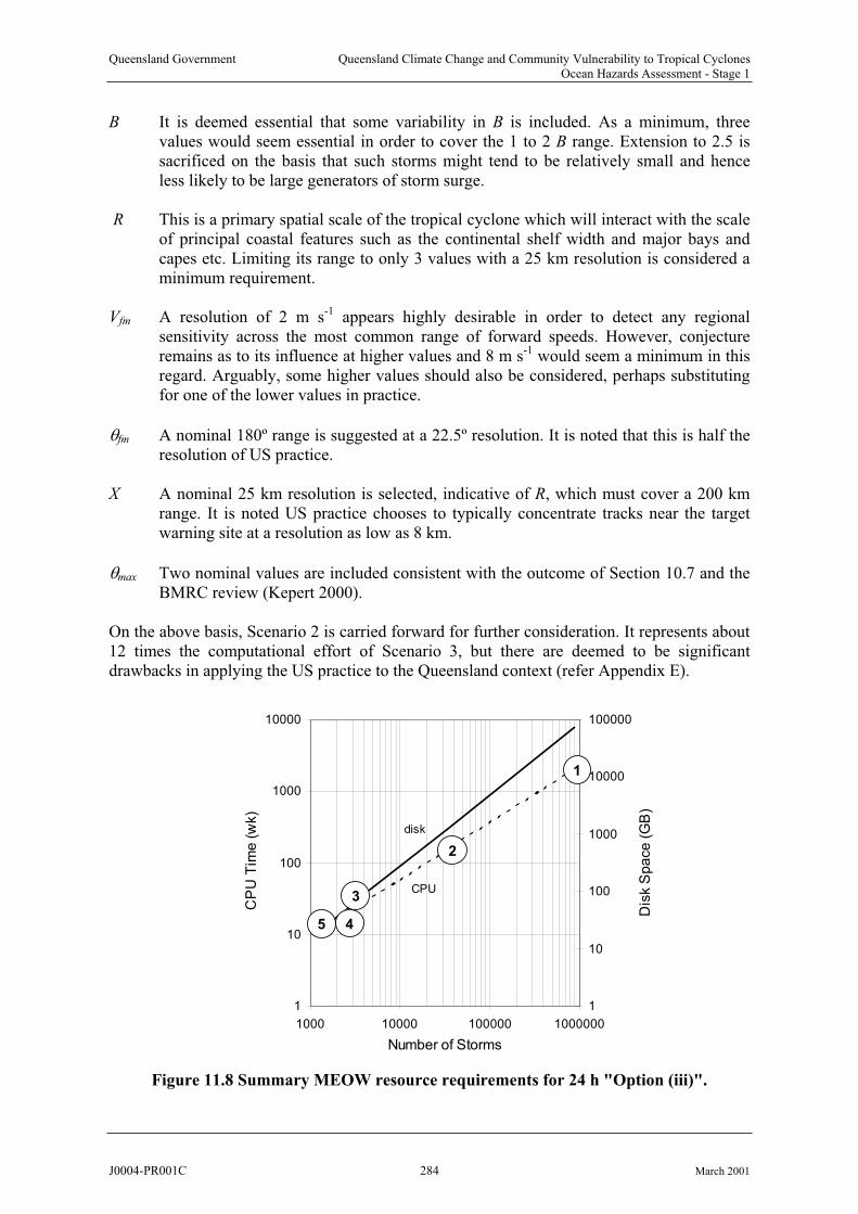
Queensland Government Queensland Climate Change and Community Vulnerability to Tropical CyclonesOcean Hazards Assessment - Stage 1
B It is deemed essential that some variability in B is included. As a minimum, threevalues would seem essential in order to cover the 1 to 2 B range. Extension to 2.5 is sacrificed on the basis that such storms might tend to be relatively small and henceless likely to be large generators of storm surge.
R This is a primary spatial scale of the tropical cyclone which will interact with the scale of principal coastal features such as the continental shelf width and major bays and capes etc. Limiting its range to only 3 values with a 25 km resolution is considered a minimum requirement.
Two nominal values are included consistent with the outcome of Section 10.7 and the BMRC review (Kepert 2000).
Vfm A resolution of 2 m s-1 appears highly desirable in order to detect any regional sensitivity across the most common range of forward speeds. However, conjecture remains as to its influence at higher values and 8 m s-1 would seem a minimum in this regard. Arguably, some higher values should also be considered, perhaps substituting for one of the lower values in practice.
fm A nominal 180º range is suggested at a 22.5º resolution. It is noted that this is half theresolution of US practice.
X A nominal 25 km resolution is selected, indicative of R, which must cover a 200 km range. It is noted US practice chooses to typically concentrate tracks near the target warning site at a resolution as low as 8 km.
max
On the above basis, Scenario 2 is carried forward for further consideration. It represents about12 times the computational effort of Scenario 3, but there are deemed to be significantdrawbacks in applying the US practice to the Queensland context (refer Appendix E).
1
10
100
1000
10000
1000 10000 100000 1000000
Number of Storms
CP
U T
ime
(w
k)
1
10
100
1000
10000
100000
Dis
k S
pa
ce
(GB
)
1
2
3
45
disk
CPU
Figure 11.8 Summary MEOW resource requirements for 24 h "Option (iii)".
J0004-PR001C 284 March 2001
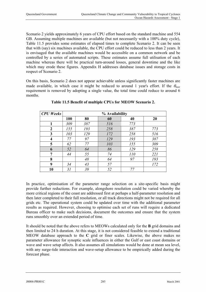
Queensland Government Queensland Climate Change and Community Vulnerability to Tropical CyclonesOcean Hazards Assessment - Stage 1
Scenario 2 yields approximately 6 years of CPU effort based on the standard machine and 554 GB. Assuming multiple machines are available (but not necessarily with a 100% duty cycle),Table 11.5 provides some estimates of elapsed times to complete Scenario 2. It can be seenthat with (say) six machines available, the CPU effort could be reduced to less than 2 years. It is envisaged that the available machines would be accessible on a common network and be controlled by a series of automated scripts. These estimates assume full utilisation of eachmachine whereas there will be practical turn-around losses, general downtime and the likewhich may erode these figures. Appendix H addresses database issues and storage costs inrespect of Scenario 2.
On this basis, Scenario 2 does not appear achievable unless significantly faster machines are
made available, in which case it might be reduced to around 1 year's effort. If the max
requirement is removed by adopting a single value, the total time could reduce to around 6 months.
Table 11.5 Benefit of multiple CPUs for MEOW Scenario 2.
CPU Weeks
No. CPUs 100 80 60 40 20
1 309 387 516 1547
2 155 193 258 387 773
3 103 129 172 258 516
4 77 97 129 193 387
5 62 77 103 155 309
6 52 64 86 129 258
7 44 55 74 110
39 48 64 97 193
9 34 43 86 172
10 31 39 52 155
% Availability
773
221
8
57
77
In practice, optimisation of the parameter range selection on a site-specific basis mightprovide further reductions. For example, alongshore resolution could be varied whereby the more critical regions of the coast are addressed first at perhaps a half-parameter resolution and then later completed to their full resolution, or all track directions might not be required for all grids etc. The operational system could be updated over time with the additional parameterresults as required. However, choosing to optimise each set of runs will require a dedicatedBureau officer to make such decisions, document the outcomes and ensure that the system runs smoothly over an extended period of time.
It should be noted that the above refers to MEOWs calculated only for the B grid domains and then limited to 24 h duration. At this stage, it is not considered feasible to extend a traditionalMEOW database approach to the C grid or finer scales. Likewise, the above makes no parameter allowance for synoptic scale influences in either the Gulf or east coast domains or wave and wave setup affects. It also assumes all simulations would be done at mean sea level, with any surge-tide interaction and wave-setup allowance to be empirically added during the forecast phase.
J0004-PR001C 285 March 2001
Queensland Government Queensland Climate Change and Community Vulnerability to Tropical CyclonesOcean Hazards Assessment - Stage 1
11.6 Conclusions and Recommendations
This section has examined the system design considerations for storm tide prediction, building on the individual recommendations from Chapters 3 through 9 and the outcomesfrom Chapter 10. The proposed MEOW technique for enabling conservative forecasts of storm tide in a warning environment was examined and compared with present US practice. The requirements in support of developing long-term storm tide statistics for planning
environments was also considered, and found to have many elements in common with the forecasting environment. A hybrid approach was then suggested as a means of ensuring bothrequirements can be satisfied in an efficient and consistent way.
Consistent with the scope of work requirement, a series of model domains for conducting storm surge calculations along the entire Queensland coast were developed and estimates of MMUSURGE runtimes on the CIRRUS1 workstation were presented. Next, a number of traditional MEOW scenarios were proposed to enable coverage of the whole State in a consistent manner and the total computing resources (time and storage) were estimated.
It is concluded that a traditional MEOWs database approach relying on essentially a priori
sets of permutations of parameters and using a primitive equation model, is not practical foraddressing the needs of the whole Queensland coast, unless it is acceptable to stage thedevelopment and extend the analyses over many years. A very large computational effort would be required, not just for the A and B grid simulations, but for subsequent fine scale simulations which will ultimately be needed to provide more specific detail at sites of interest.Currently envisaged storm surge MEOW data sets alone will also not deliver wave setupestimates and separate wave modelling will be required which, if performed to the sameformat, would be prohibitively time consuming and generate extremely large data sets.
The recommended technique for delivering the most accurate warning of storm tides is real-
time storm surge and wave prediction, fully integrated into Bureau of Meteorology
operational systems. However, the computational requirements to achieve this are significant
and this goal may take some further years of effort to complete. The alternative solution
recommended for immediate warning requirements and for use as a preparedness tool, is a
parametric storm tide model developed on the basis of a MEOWs approach, which when
combined with detailed climatology descriptions, will have direct application also for
enhanced Greenhouse climate change and storm tide statistics analyses. It is further
recommended that such a parametric model be designed to be operationally equivalent to a
MEOWs scenario environment whereby forecast perturbation analysis is based on expected
trends and error bands.
It is recommended that the parametric models so developed then be applied in conjunction
with a climatology description via a Monte Carlo Method (MCM) to provide estimates of
long-term storm tide statistics for use in evacuation and land use planning, and the protection
of environmental values. This approach should aim to provide statistics of (i) extreme storm
surge magnitudes; (ii) extreme wave heights and periods; (iii) wave setup and (iv) combined
storm tide levels. Furthermore, joint probability estimates of all parameters should also be
developed.
If a MEOW data set approach is preferred over parametric models, it is recommended that
storm tide statistics be developed using the Joint Probability Method (JPM). In this case,
J0004-PR001C 286 March 2001
Queensland Government Queensland Climate Change and Community Vulnerability to Tropical CyclonesOcean Hazards Assessment - Stage 1
relevant water level responses would be derived directly from a selection of MEOW data sets
and their probability quantum allocated based on the climatology information.
It is envisaged that development of regional parametric storm tide models would initiallyparallel a MEOW data generation step strategy, but only as many surge and wave simulationsas needed to obtain sufficient accuracy would be undertaken in each region. A relatively crudeparameter set would be chosen first, then the initial model would be developed and tested using primitive equation modelling (storm surge and waves) to the C grid level. Full datasets could then be retained for possible future project uses. Further parameter selection would then be initiated if accuracy failed to meet defined criteria. This iterative design approach will automatically be sensitive to regional non-linearities and scale interactions such that somedomains will require more complex models than others will. In addition, as a result offollowing this methodology, knowledge will be gained about the dynamics of storm tide behaviour in each region, which might otherwise become subsumed under the weight of data in a traditional MEOWs data generation step. At least an order of magnitude reduction in computational effort over the traditional MEOW would be the target outcome. Operationally,very low data requirements are expected, with the parametric models able to execute on any personal computer and be contained within a single CDROM.
GCCC (1999) 1999 Planning scheme – background study paper flooding review. Gold Coast City Council Planning Scheme, Gold Coast City Council.
Harper B.A. (1983) Half Tide Tug Harbour extreme water level study. Report prepared by Blain Bremner and Williams Pty Ltd for DBCT-UDC Joint Venture. Sept.
Harper B.A. and McMonagle C.J. (1985) Storm tide statistics - methodology. Report prepared by Blain Bremner and Williams Pty Ltd for the Beach Protection Authority Queensland, Jan.
It is further envisaged that a systematic model development process would be ideally investigated by undertaking an initial pilot study for a specific domain. This would providethe detailed methodology for application to other areas and allow the process to becomeroutinely applied for the other domains. An ability to extend the methodology to other Australian regions in a timely manner is also seen as highly desirable. The parametricapproach is also believed to be the only viable method for incorporating synoptic scale influences and the like, by significantly limiting the MEOW case studies that might normallyhave to be considered.
11.7 References
BoM (1999) The MAPINFO MEOWS (storm surge) gis display program. Prepared by A.Smallegange, Bureau of Meteorology, Queensland Regional Office, Jul, 10pp.
FEMA et al. (1999) Northwest Florida hurricane evacuation study. Prep by FEMA, NOAA,
State of Florida and US Army Corps of Engineers, July.
Harper B.A. (1996) Risk modelling of cyclone losses, Proc IEAust Annual Engin Conf,IEAust, Darwin, Apr, 53-88.
J0004-PR001C 287 March 2001
Queensland Government Queensland Climate Change and Community Vulnerability to Tropical CyclonesOcean Hazards Assessment - Stage 1
Jarvinen B.R. and Lawrence M.B. (1985) An evaluation of the SLOSH storm-surge model.Bull. Am. Met. Soc., 66(11),1408-1411.
Mason L.B. and McConochie J.D. (2001) MMUSURGE user's guide. School of Engineering, Marine Modelling Unit, James Cook University, Townsville.
Kepert J.D. (2000) Review of tropical cyclone surface windfield modelling. Prepared by Bureau of Meteorology Research Centre on behalf of Queensland Regional Office and at the request of Systems Engineering Australia Pty Ltd, Nov.
Nickerson J.W. (1971) Storm surge forecasting. Navy Weather Research Facility, Tech Report 10-71.
Sanderson B., Tang Y.M., Holland G., Grimshaw R. and Woodcock F. (1995) A tropicalcyclone maximum envelope of waters (MEOW) technique. Bureau of Meteorology, BMRC Res. Rep. No. 51, Oct, 19pp.
J0004-PR001C 288 March 2001
Queensland Government Queensland Climate Change and Community Vulnerability to Tropical CyclonesOcean Hazards Assessment - Stage 1
12. Operational Considerations for a Storm Tide Forecast System
12.1 Background
Notwithstanding the actual method of computation of a MEOW storm tide warning, as discussed in the previous Chapter, it remains to propose an operational interface which will ensure that the forecast activity is carried out efficiently and effectively, with a very low probability of confusion or error. Additionally, it is essential that the resulting forecast warning information can be effectively transmitted physically and logically to the various layers of emergency management who are required to act on its advice.
Two examples of existing BoM MEOW-related systems were made available to the presentstudy for background information, together with the comprehensive assessment by Sanderson et al. (1995) as to a methodology for undertaking MEOW warnings. In addition, preliminarydesign parameters for the planned tropical cyclone module of the Australian Integrated
Forecasting System (AIFS) were made available (BoM 2000bcd).
These example systems and supporting material will be briefly evaluated for the purpose of identifying some potential pros and cons of various approaches, leading to a revised functional specification for a future comprehensive storm tide forecasting system.
12.1.1 NMOC Operational Storm Tide Model Interface
This implements the Sanderson et al. (1995) numerical storm surge model (the current "BMRC" model) for general Bureau usage through the Numerical Modelling Operations Centre. The operation of the system is described in BoM (2000a) and is a combination of database functionality (linking to bathymetry data sets and storm track parameter files), the BMRC numerical model itself and output and display routines. Additionally, a batch interfaceto the Bureau supercomputing system completes the functionality of the system. In software terms, the system utilises ORACLE™ and IDL™ database and graphical display capabilitiesrespectively.
This not a MEOW system as such but an automated (GUI) means of operating the currentBMRC storm surge model. Further development would be required to incorporate addition of tides and consideration of forecasting uncertainties and the like to generate ensemble resultsfor a full MEOW, but in theory this process can be undertaken manually by forecasters.
While reasonably comprehensive in its present form, this style of system does not appear to be ideally suited to forecast needs. For example, it requires users to make decisions about the actual model domain to be used for the computation. Besides being an additional impost on the forecaster this is a decision best made by the model designers for (a) sound physical and numerical reasons and (b) for assured consistency and recoverability of results. Also, the output style offered by the graphical routines is not sufficiently clear and simple to be applieddirectly to warnings. In essence, the system allows a non-modeller to access and operate themodel but it contains neither safeguards nor added value for the forecaster.
It is recommended that this style of storm surge model interface (regardless of the underlyinghydrodynamic model used) be limited to the development and/or testing environment and not be made available generally for forecasting purposes.
J0004-PR001C 289 March 2001

Queensland Government Queensland Climate Change and Community Vulnerability to Tropical CyclonesOcean Hazards Assessment - Stage 1
12.1.2 Queensland Regional Office MEOW Display System
This is a MAPINFO™ application created by the Queensland Regional Office (BoM 1999) as a means of displaying the ensemble results from a numerical storm surge model (such as the BMRC model). It accesses a database of model results already undertaken for Cairns, Townsville and Mackay using an earlier version of the BMRC model. While it does provide aMEOW-style capability of interpolation between parameter values, it does not yet incorporate logic which would allow explicitly for forecast parameter uncertainty or the generation orinclusion of the astronomical tide and the effects of wave setup.
The system has a range of functionality but suffers lack of generality due to the limitations ofthe host software and operationally is relatively slow due to the need to access the large MEOW model data sets. It also stops short of actually being a forecast tool and its design is biased towards display of information rather than decision making based on that information.This observation reflects more the present stage of its development rather than its envisaged potential. Nevertheless, the concept is hampered by the lack of versatility of the GIS mappingsoftware environment and the burden of large MEOW data sets.
12.1.3 Planned AIFS Tropical Cyclone Module
This is not yet an operational system, but rather a planned module extension of the AIFS environment due for completion in 2001 (BoM 2000bcd). In present specification it merelyacknowledges that an existing AIFS storm surge modelling application interface is available (NMOC) but that a MEOW application (via the present study) is expected to be added at some future time.
This AIFS extension appears to represent an evolutionary development of the original AIFS environment (J. Kelly personal communication) and a move towards use of more OpenGL software systems with implicit Internet functionality (e.g. use of VisAD8 Java applets etc).Accordingly it is assumed more proprietary display software such as MAPINFO™ and IDL™ will be progressively phased out.
Given that this system is presently under development, it is recommended that any operational MEOW application be designed for this environment. Accordingly, issues such as databaseoperability, licencing, maintenance costs, hardware dependency etc (as required to be addressed in the scope of work; Appendix A) are best deferred to the custodians of the planned operating environment. In essence, this appears to presently favour use ofORACLE™ and VisAD environments.
Based on the information provided, there is no reason to expect that a suitable MEOWapplication could not be developed for this environment. Depending on the actual form of implementation (traditional MEOW, parametric or real-time model) efficiency requirementsmay dictate specific computational modules to be provided in, for example, C or FORTRAN source codes. Certainly, while a mapping capability is needed for interaction and display, survey accuracy in that role is not required and so traditional GIS software is neither essential nor necessarily desirable.
8 VisAD is an open source Java component library created jointly by the University of Wisconsin-Madison; the NationalCentre for Atmospheric Research (UCAR) and the NCSA. The name VisAD is an acronym for "Visualization for AlgorithmDevelopment"; refer http://www.ssec.wisc.edu/~billh/visad.html#intro
J0004-PR001C 290 March 2001
Queensland Government Queensland Climate Change and Community Vulnerability to Tropical CyclonesOcean Hazards Assessment - Stage 1
The advantage of the AIFS module environment will be that the basic operational, display andreporting functionality will be already provided and the MEOW module design can focus on delivering specific high value-added storm tide forecast products.
12.1.4 Existing Sanderson et al. (1995) Methodology
12.2 Functional Specification
12.2.2 Scope
Provision of an accurate and convenient generalised software tool based on the MaximumEnvelope of Waters (MEOW) technique for the forecasting of tropical cyclone storm tide events in Australian waters for emergency management purposes. Figure 12.1 provides a schematic overview of the intended system.
The Sanderson et al. document presents a comprehensive summary of the traditional MEOWapproach after Jarvinen and Lawrence (1985) with suggested application to the Mackay region of Queensland. It provides an overview of the philosophy and a formalisedmathematical description of the basic technique, advocating simple linear interpolationmethods provided the parameter space is shown to be adequate for the region in question. In general, these recommendations are endorsed; the suggested nominal parameter spaces beingsimilar to those independently devised herein in Chapter 11. It is noted that concerns about the potential computational burden of the traditional approach are also raised and emphasis is placed on ensuring the regional response characteristics are investigated. In this regard, the approach is similar to that recommended here in regard to the staged development of a parametric model.
However, one essential departure from the overall technique outlined by Sanderson et al. is recommended here. This relates to the order in which the final MEOW is assembled. WhereasSanderson et al. refers to undertaking forecast parameter uncertainty analysis to determine the maximum envelope of (surge) waters and subsequently adding the predicted tide, it remainsimportant to retain the variability in the tide signal as well to ensure the total (storm tide) water level is detected. Importantly, the tide phase variability is subject to the forecast parameter error in track speed and direction.
The suggested use of standard deviation uncertainty estimates of forecast parameters by Sanderson et al. is also supported, but these could be additionally augmented by user-suppliedprobability distribution estimates, as detailed later, to provide event-specific judgement.
12.2.1 Background
During the approach of a tropical cyclone towards the coast or other threatened location, interest centres on the immediate 12 h forecast position. The intensity and size of the storm is likely to be known with greater certainty than its immediate track (J. Callaghan, pers comm).Errors in the forecast track then not only spatially alter the target landfall position but can alsosignificantly alter the timing of the landfall and accordingly the relative phase between the predicted astronomical tide and the storm surge. The MEOW forecast system needs to befocused towards this critical 12 h look-ahead period and provide succinct guidance in an efficient and easy to use software environment.
J0004-PR001C 291 March 2001
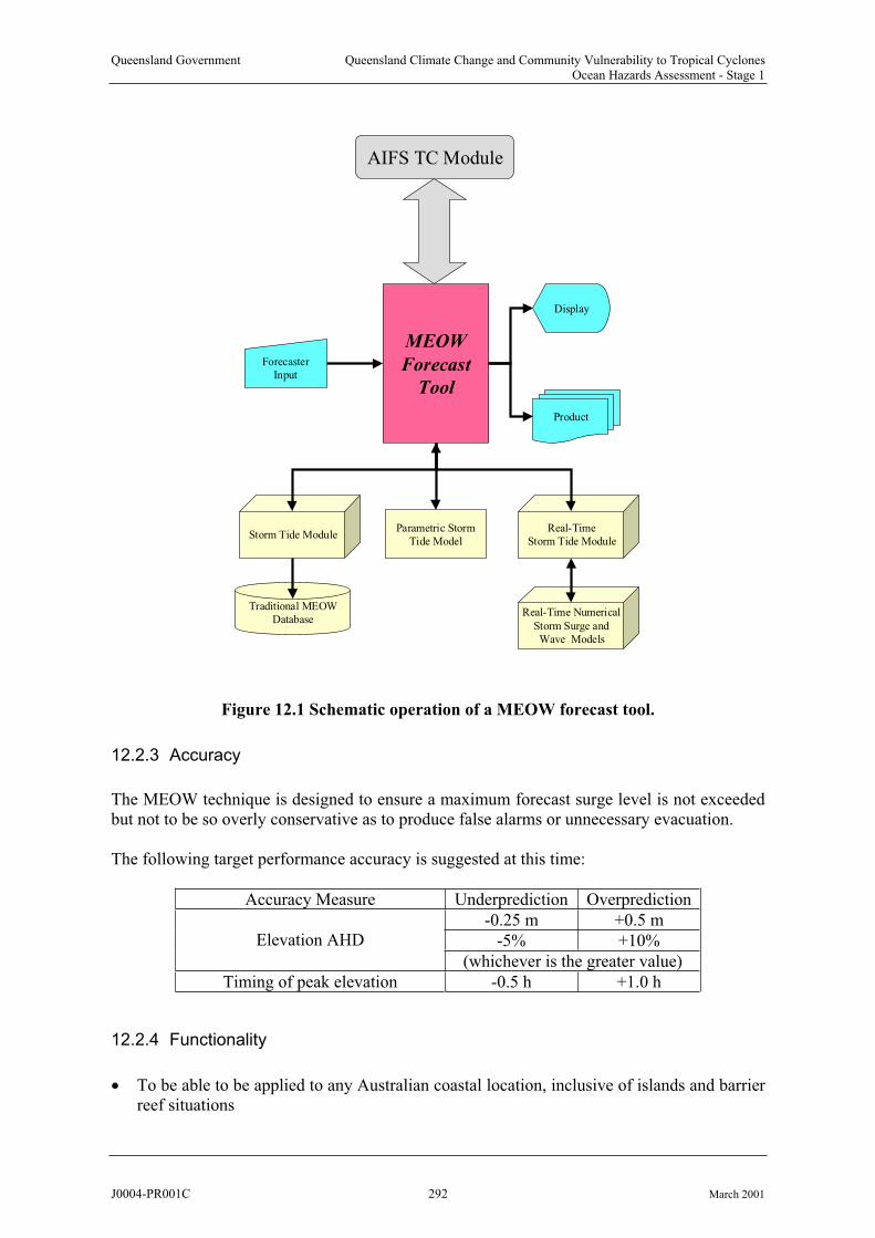
Queensland Government Queensland Climate Change and Community Vulnerability to Tropical CyclonesOcean Hazards Assessment - Stage 1
Storm Tide Module
AIFS TC Module
MEOW
Forecast
Tool
Traditional MEOWDatabase
Real-Time Numerical
Storm Surge andWave Models
Real-TimeStorm Tide Module
Display
Product
ForecasterInput
Parametric StormTide Model
Figure 12.1 Schematic operation of a MEOW forecast tool.
12.2.3 Accuracy
The MEOW technique is designed to ensure a maximum forecast surge level is not exceededbut not to be so overly conservative as to produce false alarms or unnecessary evacuation.
The following target performance accuracy is suggested at this time:
Accuracy Measure Underprediction Overprediction
-0.25 m +0.5 m
-5% +10%Elevation AHD
(whichever is the greater value)
Timing of peak elevation -0.5 h +1.0 h
12.2.4 Functionality
To be able to be applied to any Australian coastal location, inclusive of islands and barrierreef situations
J0004-PR001C 292 March 2001

Queensland Government Queensland Climate Change and Community Vulnerability to Tropical CyclonesOcean Hazards Assessment - Stage 1
To operate as an integrated tool within the AIFS tropical cyclone module environment
To be optimised for forecaster usage and forecast requirements
To calculate MEOWs in a manner which is independent of the preferred model data source (i.e. traditional, parametric or real-time)
A MEOW data source sub-system, being either or any of:
Tidal planes at all relevant sites, to include Australian Height Datum (AHD) offsets.
A matrix defining land/sea etc
surrounding ambient pressure p
-
-
To be simple and efficient in operation
To provide probabilistic MEOW estimates
To generate forecast products for distribution purposes
To provide automatic audit trail and verification statistics
12.2.5 Input Requirements
a traditional MEOW database system combined with tide and forecast uncertainty utilities
a parametric storm tide model incorporating tide and forecast uncertainty
a real-time numerical storm surge model interfaced to TCLAPS with tide and forecast uncertainty utilities and a multiple simulation batching interface
An astronomical tide database comprising:
Tidal constituents at all standard ports
Tidal phase and range offsets at all secondary ports and/or coastal localities to be warned
A geometric description of the coastline forming the warning zone, i.e.
A series of straightline approximations in 2D spatial coordinates; or
Forecast tropical cyclone track parameters (default AIFS working forecast track), to include:
minimum 24 h track duration
n hPa
pre-existing tidal anomaly9 m
storm centre fixes as appropriate, comprising: - Time t dd/mm/yyyy hh:mm UTC
- Latitude º (-ve Southern Hemisphere)
Longitude º- Central pressure p0 hPa - Radius to maximum winds R km- Holland peakedness parameter B -
Forward speed asymmetry factor* -
- Angle to maximum winds* max º * Depending on the final wind field model characteristics.
Forecast track parameter uncertainty estimates, either of:
Standard deviations of all parameters based on forecast verification studies
9 This is the actual pre-existing tidal anomaly before the storm tide is computed, normally caused by larger scale persistent or previous weather systems. It may be positive or negative but will generally be less than 0.3 m inmagnitude. This value will need to be obtained operationally from the relevant State authority, e.g. QueenslandTransport - Maritime Section or EPA Environment and Technical Services.
J0004-PR001C 293 March 2001
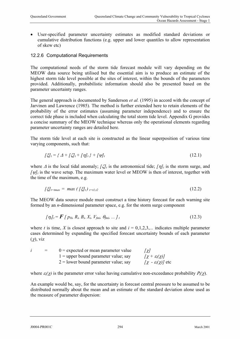
Queensland Government Queensland Climate Change and Community Vulnerability to Tropical CyclonesOcean Hazards Assessment - Stage 1
User-specified parameter uncertainty estimates as modified standard deviations or cumulative distribution functions (e.g. upper and lower quantiles to allow representation of skew etc)
12.2.6 Computational Requirements
The computational needs of the storm tide forecast module will vary depending on the MEOW data source being utilised but the essential aim is to produce an estimate of the highest storm tide level possible at the sites of interest, within the bounds of the parametersprovided. Additionally, probabilistic information should also be presented based on the parameter uncertainty ranges.
The general approach is documented by Sanderson et al. (1995) in accord with the concept ofJarvinen and Lawrence (1985). The method is further extended here to retain elements of the probability of the error estimates (assuming parameter independence) and to ensure thecorrect tide phase is included when calculating the total storm tide level. Appendix G provides a concise summary of the MEOW technique whereas only the operational elements regarding parameter uncertainty ranges are detailed here.
The storm tide level at each site is constructed as the linear superposition of various timevarying components, such that:
[ ]t = { + [ ]t + [ ]t } + [ ]t (12.1)
where is the local tidal anomaly; [ ]t is the astronomical tide; [ ]t is the storm surge, and
[ ]t is the wave setup. The maximum water level or MEOW is then of interest, together with the time of the maximum, e.g.
[ ]t=tmax = max ( [ ]t ) t=t1,t2 (12.2)
The MEOW data source module must construct a time history forecast for each warning site formed by an n-dimensional parameter space, e.g. for the storm surge component
[ i]t = F [ p0i, Ri, Bi, Xi, Vfmi, fmi, ... ] t (12.3)
where t is time, X is closest approach to site and i = 0,1,2,3,... indicates multiple parametercases determined by expanding the specified forecast uncertainty bounds of each parameter
( ), viz
i = 0 = expected or mean parameter value [ ]
1 = upper bound parameter value; say [ + i( )]
2 = lower bound parameter value; say [ - i( )] etc
where i( ) is the parameter error value having cumulative non-exceedance probability i( ).
An example would be, say, for the uncertainty in forecast central pressure to be assumed to bedistributed normally about the mean and an estimate of the standard deviation alone used as the measure of parameter dispersion:
J0004-PR001C 294 March 2001
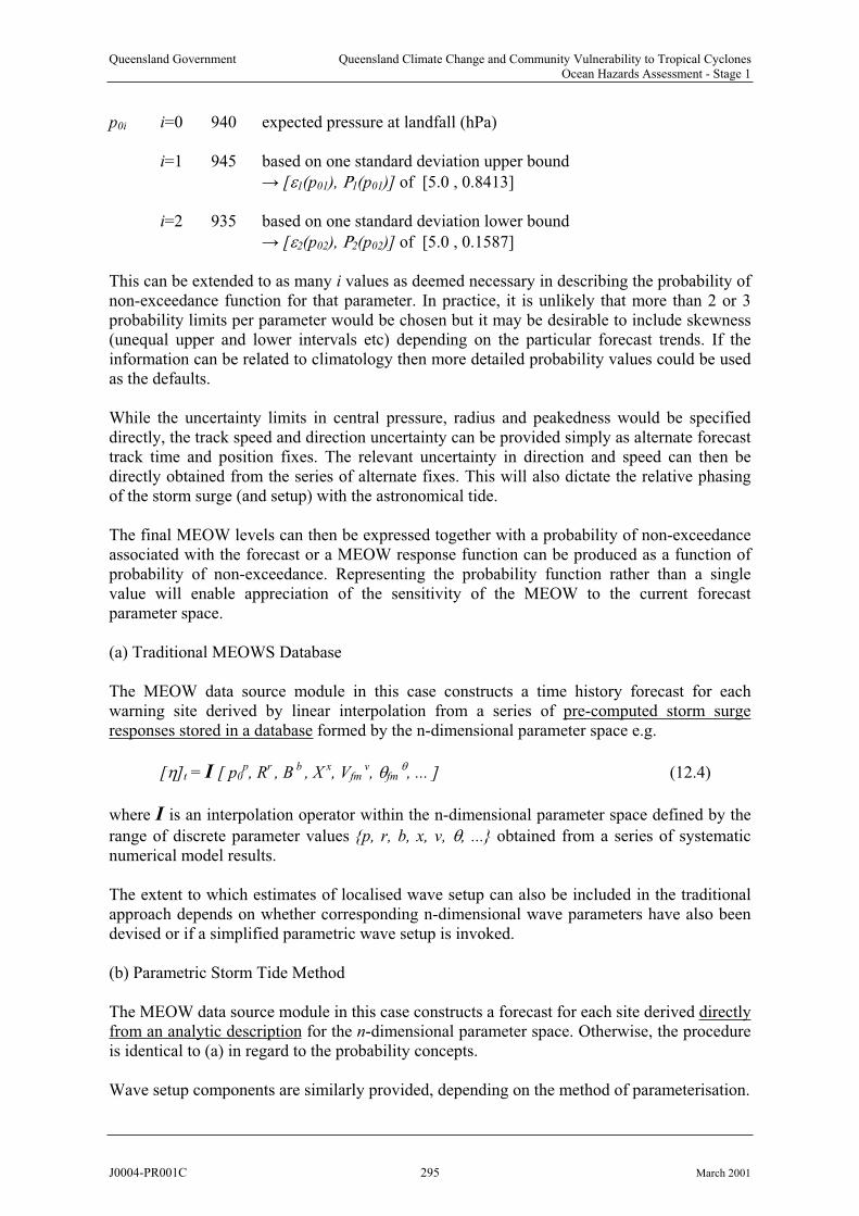
Queensland Government Queensland Climate Change and Community Vulnerability to Tropical CyclonesOcean Hazards Assessment - Stage 1
p0i i=0 940 expected pressure at landfall (hPa)
i=1 945 based on one standard deviation upper bound
[ 1(p01), 1(p01)] of [5.0 , 0.8413]
i=2 935 based on one standard deviation lower bound
[ 2(p02), 2(p02)] of [5.0 , 0.1587]
This can be extended to as many i values as deemed necessary in describing the probability of non-exceedance function for that parameter. In practice, it is unlikely that more than 2 or 3 probability limits per parameter would be chosen but it may be desirable to include skewness(unequal upper and lower intervals etc) depending on the particular forecast trends. If the information can be related to climatology then more detailed probability values could be usedas the defaults.
While the uncertainty limits in central pressure, radius and peakedness would be specified directly, the track speed and direction uncertainty can be provided simply as alternate forecast track time and position fixes. The relevant uncertainty in direction and speed can then bedirectly obtained from the series of alternate fixes. This will also dictate the relative phasingof the storm surge (and setup) with the astronomical tide.
The final MEOW levels can then be expressed together with a probability of non-exceedanceassociated with the forecast or a MEOW response function can be produced as a function of probability of non-exceedance. Representing the probability function rather than a singlevalue will enable appreciation of the sensitivity of the MEOW to the current forecast parameter space.
(a) Traditional MEOWS Database
The MEOW data source module in this case constructs a time history forecast for each warning site derived by linear interpolation from a series of pre-computed storm surge responses stored in a database formed by the n-dimensional parameter space e.g.
[ ]t = I [ p0p, R
r, B
b, X
x, Vfm
v, fm , ... ] (12.4)
where I is an interpolation operator within the n-dimensional parameter space defined by the
range of discrete parameter values {p, r, b, x, v, , ...} obtained from a series of systematicnumerical model results.
The extent to which estimates of localised wave setup can also be included in the traditionalapproach depends on whether corresponding n-dimensional wave parameters have also been devised or if a simplified parametric wave setup is invoked.
(b) Parametric Storm Tide Method
The MEOW data source module in this case constructs a forecast for each site derived directlyfrom an analytic description for the n-dimensional parameter space. Otherwise, the procedureis identical to (a) in regard to the probability concepts.
Wave setup components are similarly provided, depending on the method of parameterisation.
J0004-PR001C 295 March 2001
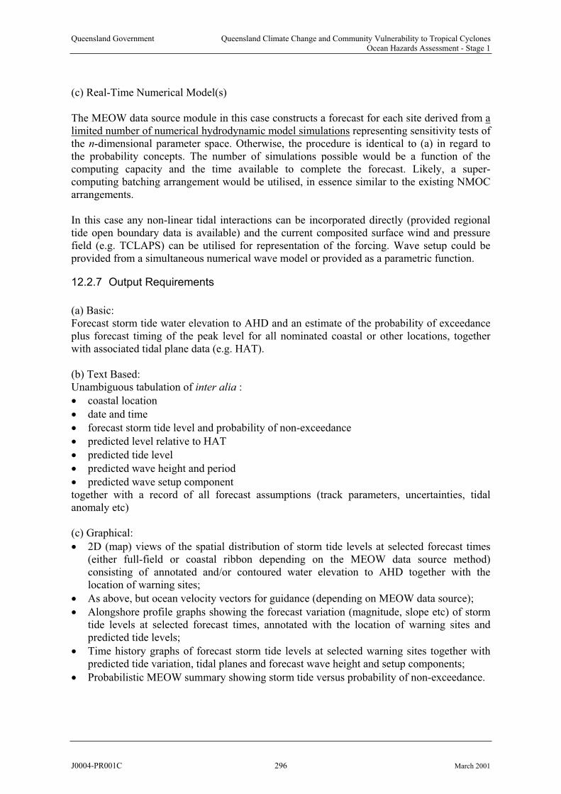
Queensland Government Queensland Climate Change and Community Vulnerability to Tropical CyclonesOcean Hazards Assessment - Stage 1
(c) Real-Time Numerical Model(s)
The MEOW data source module in this case constructs a forecast for each site derived from alimited number of numerical hydrodynamic model simulations representing sensitivity tests ofthe n-dimensional parameter space. Otherwise, the procedure is identical to (a) in regard tothe probability concepts. The number of simulations possible would be a function of the computing capacity and the time available to complete the forecast. Likely, a super-computing batching arrangement would be utilised, in essence similar to the existing NMOC arrangements.
In this case any non-linear tidal interactions can be incorporated directly (provided regional tide open boundary data is available) and the current composited surface wind and pressure field (e.g. TCLAPS) can be utilised for representation of the forcing. Wave setup could be provided from a simultaneous numerical wave model or provided as a parametric function.
12.2.7 Output Requirements
(a) Basic: Forecast storm tide water elevation to AHD and an estimate of the probability of exceedance plus forecast timing of the peak level for all nominated coastal or other locations, together with associated tidal plane data (e.g. HAT).
(b) Text Based:Unambiguous tabulation of inter alia :
coastal location
date and time
forecast storm tide level and probability of non-exceedance
predicted level relative to HAT
predicted tide level
predicted wave height and period
predicted wave setup component together with a record of all forecast assumptions (track parameters, uncertainties, tidal anomaly etc)
(c) Graphical:
2D (map) views of the spatial distribution of storm tide levels at selected forecast times(either full-field or coastal ribbon depending on the MEOW data source method)consisting of annotated and/or contoured water elevation to AHD together with the location of warning sites;
As above, but ocean velocity vectors for guidance (depending on MEOW data source);
Alongshore profile graphs showing the forecast variation (magnitude, slope etc) of stormtide levels at selected forecast times, annotated with the location of warning sites andpredicted tide levels;
Time history graphs of forecast storm tide levels at selected warning sites together with predicted tide variation, tidal planes and forecast wave height and setup components;
Probabilistic MEOW summary showing storm tide versus probability of non-exceedance.
J0004-PR001C 296 March 2001

Queensland Government Queensland Climate Change and Community Vulnerability to Tropical CyclonesOcean Hazards Assessment - Stage 1
12.2.8 Forecast Products
A range of forecast products could be produced, tailored to suit the specific client groupingsand their information needs. These might include replica output to that described above, derivative products stripped of extraneous detail to focus on a specific response role or be value-added products. Possible examples include:
Simple summary tabulations of forecast locations, times and levels
2D map views of forecast alongshore storm tide levels at the time of peak forecast levels
As above but with forecast times of storm force winds, overlaid traffic routes etc
12.2.9 Use Cases
The following are preliminary Use Cases provided to illustrate the basic envisaged operation of the forecast system. Further detailed Use Cases should be developed as necessary to fully describe the system. The following assumes a working forecast track is available which contains the additional storm parameters required for a storm tide forecast.
USE CASE 1 Specify forecast track uncertainty parameter ranges
Trigger Initial forecast or modified storm tide forecast
Description Step Action
1 Select forecast parameter of interest (e.g. track fix)
2 Select method of error estimate (std dev, CDF ordinate pairs)
3 Edit error estimates to match present expectations and limits
4 Save current parameter settings
USE CASE 2 Produce storm tide forecast
Trigger Scheduled advice due, or Trial advice required
Description Step Action
1 Select preferred storm track file (default working track)
2 Confirm or edit current parameter error estimates
3 Calculate MEOW or initiate batch run
4 Generate storm tide forecast output
USE CASE 3 Generate storm tide forecast output
Trigger Scheduled advice due, or Trial advice required
Description Step Action
1 Select type of output required (tabular, graphical etc)
2 Select time (fix or range)
3 Select warning site(s)
4 Print or display results
12.2.10 Associated Tools
(a) An Operational Parametric Windfield Model
In the cases of non-real-time simulation of MEOWs, the specification of the forecast stormtrack parameters is likely to require additional guidance, especially in regard to consistent
J0004-PR001C 297 March 2001
Queensland Government Queensland Climate Change and Community Vulnerability to Tropical CyclonesOcean Hazards Assessment - Stage 1
pairing of R and B values, forward speed asymmetry and the like. A real-time parametric windfield model with linked access to AWS data would be highly beneficial in ensuring theseparameters are wholly consistent. The model could also be used to provide direct quantitative assistance in the prediction of time of onset of gales and the extent of the warning zones etc. Such a facility would provide a base quantitative best-track documentation to enable futureverification/hindcast studies of the storm tide forecasting system.
(b) An Astronomical Tide Generator
Notwithstanding the fact that the MEOW output is specified to also indicate the predicted tide levels, this could be a useful tool to produce simple graphs and tabulations of the predicted astronomical tide to supplement the more basic information available from published tide tables.
(d) Forecast Verification Tools
(c) CLIPER Model Improvements
The specification of track parameter uncertainty estimates could benefit from an updated and/or revised CLIPER statistical model to provide objective track guidance.
These could lead to direct estimates of forecast parameter uncertainties as a function of various prediction scenarios (e.g. rapidly deepening, shearing, trough interaction etc) which could be invoked as required.
12.3 Conclusions and Recommendations
A number of existing (interim) Bureau of Meteorology storm tide warning systems and/or proposals have been examined, together with present US practice. It is concluded that none of these approaches will deliver a reliable operational forecast system without significant modification or enhancement. Furthermore, it is concluded that the present US practice forconstructing MEOW-based warnings would not be suitable for Queensland because of itsneglect of tide magnitude and phasing issues.
A functional specification was developed which would include the necessary technical features of a MEOW warning system and provide a practical forecast environment integratedinto the AIFS system. The functional specification was developed to be independent of the actual MEOW data source being used (i.e. traditional data set, parametric model or real-timemodel). Appendix G is further provided as a detailed technical description of constructing a MEOW warning.
It is recommended that a detailed MEOW-based storm tide forecast system design
specification now be prepared which will preserve tidal phase and surge relationships,
incorporate probabilistic parameter estimates and allow a selection of data source modules
(i.e. traditional, parametric or real-time).
J0004-PR001C 298 March 2001
Queensland Government Queensland Climate Change and Community Vulnerability to Tropical CyclonesOcean Hazards Assessment - Stage 1
12.4 References
BoM (2000a) Storm surge system user guide. Bureau of Meteorology, NMOC, 6pp.
Sanderson B., Tang Y.M., Holland G., Grimshaw R. and Woodcock F. (1995) A tropicalcyclone maximum envelope of waters (MEOW) technique. Bureau of Meteorology, BMRC Res. Rep. No. 51, Oct, 19pp.
BoM (1999) The MAPINFO MEOWS (storm surge) gis display program. Prepared by A.Smallegange, Bureau of Meteorology, Queensland Regional Office, Jul, 10pp.
BoM (2000b) SPB/COSB Tropical cyclone module: project plan. http://www2.bom.gov.au/sect_info/tcmodule/project_goals/project_plan.htm, Bureau of Meteorology, Apr, 7pp.
BoM (2000c) SPB/COSB Tropical cyclone module: function requirements.http://www2.bom.gov.au/sect_info/tcmodule/project_goals/function-require.htm, Bureau of
Meteorology, Mar, 7pp.
BoM (2000d) SPB/COSB Tropical cyclone module: use cases. http://www2.bom.gov.au/sect_info/tcmodule/project_goals/use_cases.htm, Bureau of
Meteorology, Oct, 9pp.
Jarvinen, B.R., and Lawrence, M.B. (1985). An evaluation of the Slosh storm-surge model.Bulletin of the American Meteorological Society, 66, 1408–1411.
J0004-PR001C 299 March 2001
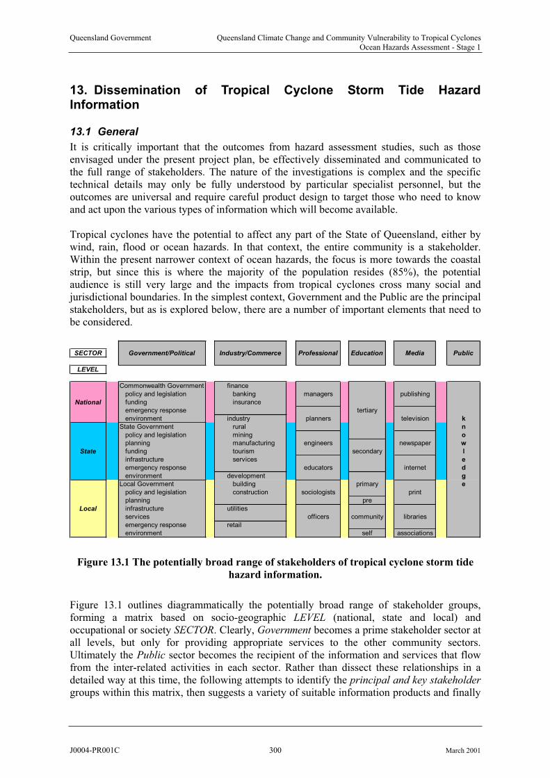
Queensland Government Queensland Climate Change and Community Vulnerability to Tropical CyclonesOcean Hazards Assessment - Stage 1
13. Dissemination of Tropical Cyclone Storm Tide Hazard Information
13.1 General
It is critically important that the outcomes from hazard assessment studies, such as thoseenvisaged under the present project plan, be effectively disseminated and communicated tothe full range of stakeholders. The nature of the investigations is complex and the specific technical details may only be fully understood by particular specialist personnel, but the outcomes are universal and require careful product design to target those who need to know and act upon the various types of information which will become available.
Tropical cyclones have the potential to affect any part of the State of Queensland, either by wind, rain, flood or ocean hazards. In that context, the entire community is a stakeholder.Within the present narrower context of ocean hazards, the focus is more towards the coastal strip, but since this is where the majority of the population resides (85%), the potential audience is still very large and the impacts from tropical cyclones cross many social andjurisdictional boundaries. In the simplest context, Government and the Public are the principal stakeholders, but as is explored below, there are a number of important elements that need tobe considered.
SECTOR Government/Political Industry/Commerce Professional Education Media Public
LEVEL
Commonwealth Government finance
policy and legislation banking managers publishing
National funding insurance
emergency response tertiary
environment industry planners television k
State Government rural n
policy and legislation mining o
planning manufacturing engineers newspaper w
State funding tourism secondary l
infrastructure services e
emergency response educators internet d
environment development g
Local Government building primary e
policy and legislation construction sociologists print
planning pre
Local infrastructure utilities
services officers community libraries
emergency response retail
environment self associations
Figure 13.1 The potentially broad range of stakeholders of tropical cyclone storm tide
hazard information.
Figure 13.1 outlines diagrammatically the potentially broad range of stakeholder groups, forming a matrix based on socio-geographic LEVEL (national, state and local) andoccupational or society SECTOR. Clearly, Government becomes a prime stakeholder sector at all levels, but only for providing appropriate services to the other community sectors. Ultimately the Public sector becomes the recipient of the information and services that flow from the inter-related activities in each sector. Rather than dissect these relationships in a detailed way at this time, the following attempts to identify the principal and key stakeholder
groups within this matrix, then suggests a variety of suitable information products and finally
J0004-PR001C 300 March 2001
Queensland Government Queensland Climate Change and Community Vulnerability to Tropical CyclonesOcean Hazards Assessment - Stage 1
proposes a match between each sector grouping and the information product type. It isexpected that subsequent detailed product design would need to involve information and communication professionals as well as social scientists, working with the base informationcreators e.g. professional engineers and/or physical scientists.
13.2 Principal Stakeholder Groups
These are identified below in the general sectoral groupings from Figure 13.1 and provided here as an information resource to provide initial guidance to others for future design and dissemination of various information products.
13.2.1 Government/Political
Identified stakeholders here include, in alphabetical order by Departments:
(a) Commonwealth Government
Department of Defence Australian Army
Emergency Management Australia (EMA)Royal Australian Navy (RAN)
Department of Environment and HeritageBureau of Meteorology
Regional OfficesQTCCC
TCWCsFWCsNMOCNCCBMRC
Great Barrier Reef Marine Park Authority (GBRMPA)Marine Group
Coastal and Marine PlanningCoasts and Clean SeasCoastcareAustralian Coastal Atlas
Australian Greenhouse Office (AGO)Department of Industry, Science and Resources
Australian Geological Survey Organisation (AGSO)Cities Project
Australian Institute of Marine Science (AIMS)Commonwealth Scientific and Industrial Research Organisation (CSIRO)
Atmospheric ResearchMarine research
Cooperative Research CentresDepartment of Transport and Regional Services
Australian Maritime Safety Authority (AMSA) Australian Transport Safety Bureau (ATSB)Local GovernmentAustralia's Territories
(b) State Government (Queensland only)
Department of Communication, Information, Local Government, Planning and SportCommunication and InformationBoard of Professional Engineers
J0004-PR001C 301 March 2001

Queensland Government Queensland Climate Change and Community Vulnerability to Tropical CyclonesOcean Hazards Assessment - Stage 1
Building CodesRegional and Urban Planning
Education Queensland (EQ)Queensland School Curriculum Council (QSCC)
Department of Emergency Services (DES)Disaster Policy and ResearchState Emergency Service (SES)State Counter Disaster Organisation (SCDO)
Environmental Protection Agency (EPA)Beach Protection Authority Coasts and WaterwaysEnvironmental and Technical Services
Department of Main Roads (DMR)Strategic Policy and developmentRoad System and Engineering
Department of Mines and Energy (DME)EnergexErgon EnergyPowerlink
Department of Natural Resources and Mines (NRM)Resource Sciences and Knowledge LandsQSIIC/QSID
Department of Primary Industries (DPI)QCCA
Department of Public Works (DPW)Queensland Transport (QT)
MaritimePlanning and Projects
Department of State Development (DSD)Regional DevelopmentStrategic Policy
Department of Tourism and Racing (DTR)Tourism Queensland
(c) Local Government (Queensland only)
There are 40 local government authorities with coastal boundaries in the State of Queensland.
13.2.2 Industry/Commerce
These include but may not be limited to (at all levels, Queensland specific):
Association of Consulting Engineers Australia (ACEA)Association of Consulting SurveyorsAssociation of Marine Park Tourist Operators (AMPTO)
Local Government Industry Training Advisory Body
Australian Chamber of Shipping (ACS)Australian Association of Ports and Marine Authorities (AAPMA)Australian Local Government Association (ALGA) Insurance Council of Australia (ICA)Local Government Association of Queensland Inc (LGAQ)
Queensland Chamber of Commerce and Industry (QCCI)Queensland Ports Association (QPA)
Bundaberg Port AuthorityCairns Port AuthorityGladstone Port AuthorityPort of Brisbane AuthorityPorts Corporation QueenslandTownsville Port Authority
J0004-PR001C 302 March 2001
Queensland Government Queensland Climate Change and Community Vulnerability to Tropical CyclonesOcean Hazards Assessment - Stage 1
Queensland Master Builders Association (QMBA)Queensland Tourism and Hospitality Industry Training Council IncReal Estate Institute of Queensland (REIQ) Standards Australia (SA)
13.2.3 Professional
These include but may not be limited to (at all levels, Queensland specific):
Australian Journalist's Association (AJA)Australian Institute of Management (AIM)Australian Institute of Petroleum (AIP) Australian Insurance Institute (AII) Eastern Dredging Association (EDA)Institute of Actuaries of Australia (IAA)Institute of Emergency Services (Qld) Institute of Municipal Management (Qld Div)Institute of Public Works Engineering Australia (Qld Div) Institution of Engineers, Australia (IEAust)
Queensland DivisionWater Panel
National Committee on Coastal and Ocean Engineering (NCCOE)Institution of Surveyors, Australia
Royal Australian Planning Institute (RAPI)
13.3.1
Royal Australian Institute of Architects (RAIA)
13.2.4 Education and Media
These include but may not be limited to (at all levels, Queensland specific):
UniversitiesJames Cook University
Centre for Disaster StudiesCyclone Structural Testing StationMarine Modelling UnitReef Research CRC
TAFEsSecondary SchoolsPrimary and Pre-SchoolsCommunity associations, interest groups and the like.National, State and Local LibrariesNewspaper ProprietorsTelevision Networks
13.3 The Key Stakeholders and/or Key Methods of Information Delivery
Notwithstanding the above broad stakeholdings and interest groups, specific key agencies and organisations provide the information delivery mechanisms. In the main, with the exceptionof the Bureau of Meteorology and Emergency Management Australia, these are State or Local Government organisations. Their roles and responsibilities are briefly outlined below withinthe context of either long term preparedness or short term responsiveness roles or sometimesdual roles.
Bureau of Meteorology
The Bureau of Meteorology (BoM 2000) is the National Meteorological Service for Australia, established by an Act of the Commonwealth Parliament in 1906. Its responsibilities include:
J0004-PR001C 303 March 2001
Queensland Government Queensland Climate Change and Community Vulnerability to Tropical CyclonesOcean Hazards Assessment - Stage 1
Provision of essential weather, climate and related environmental services to theAustralian community;
Meeting Australia's international obligations under the Convention of the World
Meteorological Organization and other multilateral treaty obligations to providemeteorological support for the safety of international shipping and aviation and the protection of the global atmosphere
scientific advisory and consultancy services in meteorology, hydrology and oceanography.
To review cyclone experiences and consider the measures necessary to overcomedeficiencies;
To coordinate the continuing development of tropical cyclone and storm tide warning andresponse arrangements;
Storm tide warnings are issued by the Bureau of Meteorology in conjunction with the State
Counter Disaster Organization (SCDO 2000) which interfaces with a number of key State Government organizations. The Department of Emergency Services provides the executiverole for the SCDO and the Beach Protection Authority provides specialist advice and data in respect of wave and storm surge readings from its real-time network of waverider buoys and storm surge gauges. The issuing of storm tide warnings is also staged depending on the threat and the expected onset of high winds at the affected locations, which might impede potential evacuation to higher ground.
Custodianship of the official records of Australian weather and climate;
Bureau services include:
warnings of dangerous weather such as severe thunderstorms and tropical cyclones,and weather conditions leading to floods or bush fires;
weather forecasts for the land areas and for the coasts and oceans around Australia;
seasonal outlooks of Australia's climate;
data and information services on the weather and climate of Australia and surrounding areas; and
In terms of local planning and information dissemination, the Queensland Regional Office(jointly with the Department of Emergency Services) organises and convenes the Queensland
Tropical Cyclone Coordination Committee (QTCCC) which draws membership from a wide range of government and industry organisations. The QTCCC meets quarterly, its terms ofreference being:
To advise and receive input from government authorities and other organisations on the measures necessary to reduce the impacts of tropical cyclones and related storm tides inQueensland;
To obtain advice and information, consider and make representations on any matterrelevant to the good management of cyclone and storm tide threats in Queensland;
To form special purpose working groups as necessary.
The QTCCC provides and annual report on its operations to the SCDO (see below) and the Director of Meteorology.
J0004-PR001C 304 March 2001

Queensland Government Queensland Climate Change and Community Vulnerability to Tropical CyclonesOcean Hazards Assessment - Stage 1
13.3.2 Emergency Management Australia (EMA)
EMA is the Federal agency responsible for reducing the impact of natural and human-causeddisasters on the Australian community and the lead agency for coordinating Federal disaster
response (EMA 2000). EMA reports to the Minister for Defence who has Government-wide
responsibility for emergency and disaster matters. Its key responsibilities include:
developing Commonwealth Government and national emergency managementpolicies, plans and programs;
through the Australian Emergency Management Institute, developing national emergency management education and training curriculum and programs. It also develops emergency management doctrine reflecting best practice in all facets of emergency management and fosters emergency management research;
working closely with Commonwealth Government agencies, state and territoryemergency management organisations, local government and the international community, particularly the island nations of the South Pacific;
fostering and providing disaster awareness and education materials and campaigns in conjunction with state and territory organisation;
supporting the development of Australia's civil defence capability;
providing financial support to states and territories for the development of emergencycapabilities through the Commonwealth Government's State Support Package.
13.3.3 Queensland Department of Communication, Information, Local Govt, Planning and Sport
Through Regional and Urban Planning Services (DCILGP 2000), the Departmentimplements and manages best practice planning and development assessment systems,principally through the Integrated Planning Act 1997 (IPA). The system is designed to bring all relevant State and local government approvals into one common process called the Integrated Development Assessment System (IDAS). This system focuses on achievingecologically sustainable development in Queensland, through integrated planning that balances social, economic and environmental considerations. The Department maintains thelegislative and regulatory framework for the conduct of planning and development. In partnership with key clients and stakeholders, it supports the preparation and implementationof regional planning strategies and provides an extensive range of essential planning information to meet client needs and help users of the planning system. On request, the Department also assists local governments and others to resolve land use and developmentissues.
13.3.4 Queensland Department of Emergency Services (DES)
The role of DES is to serve and support the Queensland community in preventing, planning for, responding to and recovering from emergencies and disasters (DES 2000).
Counter Disaster and Rescue Services is responsible for Queensland’s disaster managementarrangements, core staffing of the State Counter Disaster Organisation (SCDO) and the provision of emergency helicopter and chemical hazard advisory services. It is also jointconvenor of the Queensland Tropical Cyclone Coordination Committee (QTCCC), togetherwith the Bureau of Meteorology.
J0004-PR001C 305 March 2001

Queensland Government Queensland Climate Change and Community Vulnerability to Tropical CyclonesOcean Hazards Assessment - Stage 1
Disaster management services include:
Disaster policy development, planning and operational co-ordination;
Disaster management advice, training and information;
Disaster response and recovery;
Strategic whole-of-Government disaster management policy, and support to the Central Control Group (CCG), State Counter Disaster Organisation;
Liaison with Government Departments with functional and threat-specific disasterresponsibilities, the Australian Defence Force and the Local Government Association of Queensland on disaster management issues;
Disaster-related research projects.
State Emergency Service (SES) and Volunteer Marine Rescue (VMR) Operational
Preparedness:
Training support services and equipment support services to SES volunteers and StateEmergency Service Cadet Groups;
Provision of support to Australian Volunteer Coast Guard (AVCG) and VolunteerMarine Rescue Association of Queensland (VMRAQ) groups; Surf Life Saving
Queensland (SLSQ) and Royal Life Saving Society (RLSS) beach patrols.
State Counter Disaster Organisation (SCDO):
The SCDO is an umbrella organisation that encompasses all agencies, groups and officers that make up the Queensland Disaster Management System. The SCDO is only activated during times of disaster and provides assistance to Queensland communities when local resources areunavailable or have become exhausted. Local Government Counter Disaster Committees
coordinate the response to a disaster at the local level. If resources are not available locally toproperly respond to the disaster, the Local Government can request additional resources fromthe Disaster District.
13.3.5 Queensland Environmental Protection Agency (EPA)
The EPA administers the key Queensland legislation of the Environmental Protection Act
1994, the Nature Conservation Act 1992, the Marine Parks Act 1982, the Coastal Protection
and Management Act 1995 and the Queensland Heritage Act 1992 (EPA 2000a).
Divisional Roles:
Coasts and Waterways is responsible for coastal management and integrated planning for the coastal zone, including waterways and wetlands. This involves setting standards andpolicies, planning for protection and management of all aquatic, coastal, marine and wetland areas under Queensland jurisdiction. This function also supports the Beach Protection
Authority, the statutory objective of which is to regulate and provide advice in respect of certain activities affecting the coast, to protect the amenity of the coast and to minimisedamage to property from erosion or encroachment by tidal water. Planning and Assessment
co-ordinates the implementation of Integrated Planning Act (IPA) requirements covering impact assessment, state-level impact assessment and strategic assessments associated withspecial projects. Strategic Policy is responsible for major environmental policy projects which involve whole-of-government co-ordination and intergovernmental negotiations, and for managing environmental policy processes that cross jurisdictional boundaries. It managesthe development of Queensland’s Greenhouse Response Strategy and related programs,including the Queensland Greenhouse Inventory and promotion of the Greenhouse Challenge
J0004-PR001C 306 March 2001

Queensland Government Queensland Climate Change and Community Vulnerability to Tropical CyclonesOcean Hazards Assessment - Stage 1
Program. Legislation develops applied policy for the EPA and co-ordinates development ofenvironmental legislation, regulations and environmental protection policies. It also contains a Local Government Group to provide a key reference point for local governments in Queensland to liaise with the EPA on environmental issues. It is also responsible formanaging a protocol agreement with the Local Government Association of Queensland, andimplementing the EPA’s Delegations and Authorisations Policy. Economics evaluateseconomic implications of environmental policy proposals and other factors which impact on the environment. Environmental and Technical Services - Coastal Services undertakes a range of State-wide monitoring and modelling functions as well as providing expert advice on coastal processes in so far as they relate to EPA policies and strategies.
The State Coastal Plan:
The EPA is currently developing the State Coastal Plan (EPA 2000b), which is to form aframework for considering coastal management outcomes, principles and policies when undertaking planning, assessing development applications and undertaking managementdecisions. The State Coastal Plan has the effect of a State Planning Policy under the Integrated Planning Act 1997 and will be one of the matters that are coordinated and integrated into new LGA planning schemes during their preparation over the next few years. The State Coastal Plan will set a new standard for coastal management in Queensland and aims to promote consistency in the way coastal management is implemented by identifying in a single document the State’s coastal management outcomes, principles and policies. Together with regional coastal management plans it will have the force of law under the Coastal Act
and agencies and persons with responsibilities in the coastal zone that are governed by or linked to the Coastal Act, will need to have regard to the provisions of these plans. These include agencies and persons preparing plans, undertaking assessments and issuing approvals, and making management decisions.
Community Planning:
The Coastal Protection Advisory Council:
Under the Coastal Act, the Coastal Protection Advisory Council advises the Minister forEnvironment directly on coastal management matters. These matters include the developmentand implementation of coastal plans and their relationship to other plans, areas within Queensland requiring special coastal management, research and other studies relating to the coastal zone, developing public awareness and consultation programs, and assistance that local government and other agencies may need in undertaking coastal management.
13.3.6 Queensland Local Government Authorities
There are 125 Local Government Authorities (LGAs) in Queensland which, under The Local
Government Act (1993), are granted authority to enact Local Laws for the general well being and governance of the community. Within the present study context, LGAs undertake three important roles, namely:
LGA planners are responsible for preparing planning schemes under the Integrated Planning
Act 1997 taking into account matters of State and regional interest such as the State Coastal Plan and Emergency Management Plans in assessing particular development applications. Such plans may incorporate risk mitigation measures and many LGAs are currently receiving
J0004-PR001C 307 March 2001
Queensland Government Queensland Climate Change and Community Vulnerability to Tropical CyclonesOcean Hazards Assessment - Stage 1
funding assistance directly from EMA and DES in this regard to understand and reduce their long-term risk to many natural hazards.
Infrastructure Provision:
LGA engineers are responsible for the adequate design of community infrastructure (roads, bridges, water supply and sewerage, ports and marinas, beaches, building approvals,certification etc). They need to be aware of special design provisions likely to be required to ensure tropical cyclone hazards are adequately considered. This will include specific issues in regard to risk mitigation plans.
Counter Disaster:
Many coastal LGAs already maintain storm tide impact and evacuation maps which addresspresently interpretations of the tropical cyclone threat to their communities. Under theQueensland Disaster Management System, Local Government Counter Disaster Committees
coordinate the response to any disaster at the local level. If resources are not available locally to properly respond to the disaster, the Local Government can request additional resourcesfrom the Disaster District via the SCDO. The LGA emergency managers involved in (part-time) counter disaster measures are often drawn from engineering or planning divisions but may be completely separate staff members without access to the same information on tropical cyclone risks or without specific training in the interpretation of such information.
13.3.7 Industry Associations
A number of influential industry associations exist to service a wide range of needs for their member organisations. Tropical cyclone impacts and issues will figure in many aspects of their services, training and advice.
LGAs in Queensland are supported by the Local Government Association of Queensland,which provides a range of information and policy services and will be an important LGA conduit for tropical cyclone hazard information and education. Other major associations include the Association of Consulting Engineers Australia, Queensland Ports Association
(formerly Harbour Board Association) and the Queensland Master Builders Association.
In operational terms, organisations such as the Association of Marine Park Tourist Operators
may be valuable communicators of risk information to the tourism industry. Over the longer term, mitigation efforts may be strengthened by the support of the Insurance Council of
Australia, and Standards Australia provides mechanisms by which design practice can be influenced by the various professional bodies.
13.3.8 Professional Bodies
Various professional bodies provide a range of information, networking and continuing education services to individual personnel with important roles in either long-term disaster preparedness or counter disaster response.
For example, LGA engineers and planners look to their professional bodies such as the Institute of Public Works Engineering Australia (previously the Local Government Engineers Association Queensland), the Institution of Engineers, Australia (IEAust) and the Royal
J0004-PR001C 308 March 2001

Queensland Government Queensland Climate Change and Community Vulnerability to Tropical CyclonesOcean Hazards Assessment - Stage 1
Australian Planning Institute for state of practice guidance. The IEAust has Local Branch representation at Gold Coast, Sunshine Coast, Wide Bay, Gladstone, Rockhampton,Townsville and Cairns where regular meetings are held. Emergency managers, for example,are additionally served by an Institute of Emergency Services.
Many of these professional bodies conduct education and training, annual conferences and the like or produce publications which form a valuable reference source for day to day professional practice and measures of acceptable peer conduct such as duty of care.
13.4 Potential Information Products
A variety of information products could be envisaged to deliver the relevant information,advice and guidance to the full range of stakeholders. However, this needs to be specificallytargeted to each sector to maximise the information transfer value. Figure 13.2 presents anoverview of the likely match between each sector (as identified in Figure 13.1) earlier) and a range of possible information products. It is suggested that different sectors will expect and seek information in different formats and levels of detail. As illustrated, there are at least 8identifiable tiers of information that will require consideration for an effective informationstrategy.
13.4.1 Media Delivery Mechanisms
The Internet is expected to be an increasingly important media delivery mechanism becauseof its ease of access and ability to incorporate graphical and interactive tools. However, there will remain a significant requirement for traditional documentation and especially qualitycontrol and tracking procedures to ensure accurate information is always being provided todecision managers. Inclusion of essential aspects of knowledge into general school curricula should be pursued.
Final technical recommendations and procedures would ideally be enshrined into State legislation and Local Government Laws for ease of reference and enforcement.
13.4.2 Content
Within the above context, two basic information streams are also required:
Warning and response
Planning and mitigation
These information streams need to be mutually consistent and supportive to allow theinformation seeker to move freely between the two contexts. For example, local emergencymanagers should become familiar with the relative risks of inundation due to storm tide (predominantly a planning issue) when responding and reacting to actual warnings. Evacuation plans and the like should ensure that they are at least optimised to handle the morelikely scenarios whilst incorporating contingency for the ultimate event. Conversely, those having planning and design responsibility should appreciate that the ultimate event is possible and consider the likely community impacts in that situation. Economics will play a part ineach case and decision-making tools will be required to ensure consistency of approachesacross organisations and regions.
J0004-PR001C 309 March 2001
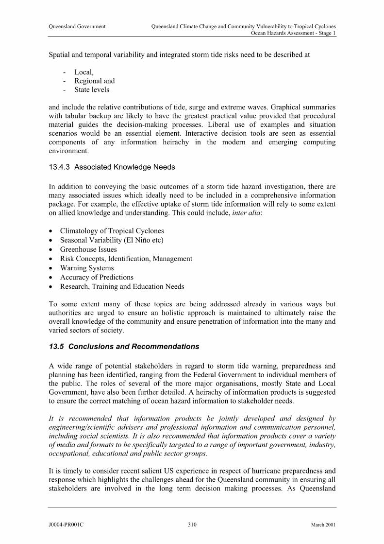
Queensland Government Queensland Climate Change and Community Vulnerability to Tropical CyclonesOcean Hazards Assessment - Stage 1
Spatial and temporal variability and integrated storm tide risks need to be described at
- Local, - Regional and- State levels
and include the relative contributions of tide, surge and extreme waves. Graphical summarieswith tabular backup are likely to have the greatest practical value provided that procedural material guides the decision-making processes. Liberal use of examples and situation scenarios would be an essential element. Interactive decision tools are seen as essential components of any information heirachy in the modern and emerging computingenvironment.
13.4.3 Associated Knowledge Needs
In addition to conveying the basic outcomes of a storm tide hazard investigation, there are many associated issues which ideally need to be included in a comprehensive informationpackage. For example, the effective uptake of storm tide information will rely to some extent on allied knowledge and understanding. This could include, inter alia:
Climatology of Tropical Cyclones
Seasonal Variability (El Niño etc)
Greenhouse Issues
Risk Concepts, Identification, Management
Warning Systems
Accuracy of Predictions
Research, Training and Education Needs
To some extent many of these topics are being addressed already in various ways but authorities are urged to ensure an holistic approach is maintained to ultimately raise theoverall knowledge of the community and ensure penetration of information into the many and varied sectors of society.
13.5 Conclusions and Recommendations
A wide range of potential stakeholders in regard to storm tide warning, preparedness and planning has been identified, ranging from the Federal Government to individual members of the public. The roles of several of the more major organisations, mostly State and Local Government, have also been further detailed. A heirachy of information products is suggested to ensure the correct matching of ocean hazard information to stakeholder needs.
It is recommended that information products be jointly developed and designed by
engineering/scientific advisers and professional information and communication personnel,
including social scientists. It is also recommended that information products cover a variety
of media and formats to be specifically targeted to a range of important government, industry,
occupational, educational and public sector groups.
It is timely to consider recent salient US experience in respect of hurricane preparedness andresponse which highlights the challenges ahead for the Queensland community in ensuring all stakeholders are involved in the long term decision making processes. As Queensland
J0004-PR001C 310 March 2001
Queensland Government Queensland Climate Change and Community Vulnerability to Tropical CyclonesOcean Hazards Assessment - Stage 1
continues its rapid development it is likely that the State will approach the types of problemsbeing experienced in the USA along the Gulf and Atlantic coasts which are subject to significant levels of hurricane attack.
The following is a precis of findings made at a recent multi-disciplinary forum organised bythe American Meteorological Society and sponsored by The Weather Channel (AMS 2000):
The nation's hurricane policy has evolved so that it depends primarily on preparedness,
prediction and evacuation and places only minimal reliance on land use strategies, structural engineering and building codes.
Strains in existing procedures are forcing new response strategies for managers away
from total reliance on comprehensive evacuations; shelter-in-place or refuge-of-last-
resort solutions are being considered which reduce response times but carry higher risk
and are yet to be fully studied and evaluated by the communities they serve.
Reliance on weather prediction and evacuation is increasingly strained by population
and economic development in coastal areas; evacuation clearance times are increasing
to the point where they exceed the lead-time of high-confidence forecasts; many people
remain in high-risk areas while the road and shelter infrastructure becomes overloaded
with people at much lower risk; local evacuation decisions are triggering mass
population movements with severe traffic congestion and shelter shortages on a
regional scale.
There is poor understanding and application of uncertainties in hurricane forecasts,
risk assessments, population responses, infrastructure capacities and media coverage;
future development of the preparedness, forecast, communications and response system
must address the full range of uncertainties.
13.6 References
AMS (2000) Policy issues in hurricane preparedness and response. Proc of The Weather Channel Forum, Developed by the Atmospheric Policy Program of the AmericanMeteorological Society, AMS, Sept.
BoM (2000) Extracted from http://www.bom.gov.au, Nov.
DCILGP (2000) Extracted from http://www.dcilgp.qld.gov.au/index_planning.html, Nov.
DES (2000) Extracted from http://emergency.qld.gov.au, Nov.
EMA (2000) Extracted from http://www.ema.gov.au/1aboutema/ataglance.html, Nov.
EPA (2000a) Extracted from http://www.env.qld.gov.au/environment/about/structure, Nov.
EPA (2000b) Extracted fromhttp://www.env.qld.gov.au/environment/coast/management/welcome.html, Nov.
SCDO (2000) Storm tide warning-response system. Jointly issued by the State Counter
Disaster Organisation and the Bureau of Meteorology (Qld).
J0004-PR001C 311 March 2001
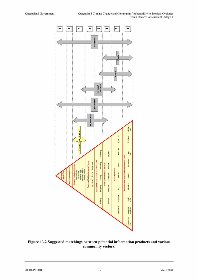
Queensland Government Queensland Climate Change and Community Vulnerability to Tropical CyclonesOcean Hazards Assessment - Stage 1
Pro
fessio
nal
Ind
ustr
y/
Co
mm
erc
e
Ed
ucati
on
Med
ia
Pu
bli
c
Pre
sen
t S
tud
y C
on
text
Go
vern
me
nt
1 2 3 4 5 6 7 8
veri
fications
decis
ion tools
recom
mendations
researc
h n
eeds
monogra
ph jo
urn
al c
onfe
rence
pla
nnin
gdesig
nin
gbuild
ing
cert
ifyin
gopera
ting
bookle
tsbro
chure
spham
ple
tsin
tern
et
stickers
new
spaper
magazin
efilm
tele
vis
ion
foru
ms
sem
inars
work
shops
info
rmation
gra
phic
al
media
education
gam
es
inte
ractive
maps
flow
chart
sdis
pla
ys
kits
pro
ducts
gra
bs
kits
tools
Deta
iled
Tech
nic
al R
ep
ort
s
meth
odolo
gie
s
Tech
nic
al P
ub
licati
on
s a
nd
Pap
ers
Execu
tive S
um
mari
es
Str
ate
gy
Do
cu
men
ts
Sta
nd
ard
s C
od
es G
uid
es
an
d P
roced
ure
s
Pu
blic In
form
ati
on
Su
mm
ari
es
Pu
blic E
du
cati
on
Med
ia R
eso
urc
es a
nd
Oth
er
Info
rmati
on
To
ols
Figure 13.2 Suggested matchings between potential information products and various
community sectors.
J0004-PR001C 312 March 2001

Queensland Government Queensland Climate Change and Community Vulnerability to Tropical CyclonesOcean Hazards Assessment - Stage 1
14. Summary Conclusions and Recommendations
This report presents the results of work undertaken in respect of the project scope for Part A:
Review of Project Technical Requirements, sub-scopes A-1 to A6, detailed below (referAppendix A for details of the project scope). Part B-1 of the project relates to the provision ofa numerical modelling system for storm surge prediction and is separately documented in the form of a User Guide and other supporting information.
Each Chapter of this report contains specific conclusions and recommendations that should bereferenced for further clarification and guidance. In respect of each Part A sub-scope, the following summary conclusions and 10 specific recommendations are made:
Scope: General
Chapter 2 introduces the concepts and definitions relevant to the assessment of ocean hazardsfrom tropical cyclones in Queensland within the context of both existing climate and thepotential for enhanced Greenhouse climate change.
Chapter 3 provides an overview of the known climatology of tropical cyclones in Queensland and considers issues of data quality and applicability for ocean hazard assessment. Thepotential influence of interseasonal (ENSO) and interdecadal (IPO) oscillations is considered.
It is recommended that a comprehensive climatology study be undertaken which will provide
a "seamless" statistical description of tropical cyclone variability across the State of
Queensland (similar to that described in Chapter 9) to be used for long term estimates of
storm tide and other impacts and also to provide guidance for real-time forecasting. Synoptic scale interactions with tropical cyclone vortices should also be considered, together with
decay after landfall, recurvature and regeneration issues.
1
2
Scope A-1: Assessment of Greenhouse climate change and sea level rise.
Chapter 4 provides a comprehensive assessment of the current state of knowledge of Greenhouse climate change and sea level rise. Special consideration is given to the possible impacts of changes in tropical cyclone characteristics in the Australian region relevant to thegeneration of storm surges, including the maximum potential intensities (MPIs) of tropicalcyclones.
It is recommended that the assessment of long-term storm tide risks to the Queensland coast
should include allowance for the current estimates of enhanced Greenhouse sea level rise and
a 10% to 20% potential increase in the MPI of tropical cyclones. Although no significant
increase in frequency of occurrence or geographical coverage is anticipated, it is considered
prudent to investigate the sensitivity of storm tide statistics to a 10% variation in these
aspects of the climatology under an enhanced Greenhouse scenario.
Scope A-2: Review the technical requirements for numerical modelling of cyclone
storm surge.
Chapter 5 provides an overview of the development and current science of analytical modelsof the tropical cyclone wind and pressure field environment relevant to the generation of
J0004-PR001C 313 March 2001
Queensland Government Queensland Climate Change and Community Vulnerability to Tropical CyclonesOcean Hazards Assessment - Stage 1
cyclone storm surge and extreme waves. It is concluded that parametric models of the tropical cyclone surface forcing are generally robust but there are aspects still requiring research anddevelopment which may significantly impact the prediction of storm tide in Queensland. Chapter 10, for example, shows a high sensitivity to wind field asymmetry assumptions.Synoptic-scale interactions with the tropical cyclone vortex will also be important in somesituations and Appendix D describes additional MMUSURGE capabilities in that regard.
It is recommended that further sensitivity testing of the impact of the latest tropical cyclone
boundary layer research (e.g. BMRC model) be undertaken by selective hindcasting and comparison with existing Australian wind data before committing to an extensive storm tide
modelling project.
3
4
5
Chapter 6 provides a comprehensive technical review of the state-of-the-art of numericalhydrodynamic modelling of tropical cyclone storm surge, which discusses the essential physics, necessary approximations, simplifications and numerical treatments. The development parallels the current status of the James Cook University Marine Modelling Unit storm surge model (MMUSURGE), the details of which are given in Appendix D.
Chapter 10 presents the results of an extensive investigation into the meteorology and oceanresponse of a number of significant historical tropical cyclone events in Queensland. Hindcasting of the storm tides has demonstrated the accuracy of the MMUSURGE model in a variety of coastal environments and over a range of tropical cyclone classes. A series of sensitivity tests has highlighted desirable parameter settings. It is concluded that the modelperforms accurately when wind and pressure data is also accurate and the domain bathymetryis reasonably well defined. Situations of extensive overland flooding, such as the Gulf of Carpentaria, are the most poorly represented in the model due to a lack of accurate data. More tidal analysis is also required to provide accurate real-time prediction of simultaneous surge and tide propagation for many areas of Queensland. These matters are not model limitationsbut simply reflect a lack of tidal data and inadequate bathymetry in many areas.
It is concluded that the numerical storm surge model MMUSURGE is capable of accurately
and efficiently modelling the generation and propagation of storm tide provided that wind
and pressure data is also accurate and that the coastal representation and other parameters
are consistent with the recommendations of Chapter 6. It is recommended that further model
calibration with improved data be undertaken to (a) ensure improved representation of
overland flooding - especially in the high-risk Gulf of Carpentaria region and (b) to
undertake further tidal calibration work to provide real-time surge and tide modelling
capability needed for inundation modelling.
Chapter 9 provides a comprehensive overview of techniques for developing storm tide statistics and the various advantages and disadvantages of a number of methods. It is concluded that three simulation methods have similar potential but differ in their needs for the description of the climatology and the extent of primitive equation modelling required.
It is recommended that the Monte Carlo Method (MCM) be adopted as the most suitable
technique for establishing storm tide statistics, assuming a parametric storm tide model is
available (refer recommendation 8). This method provides the greatest opportunity for
inclusion of a wide range of parameter sensitivities, including interseasonal, interdecadal and
climate change impacts. Alternatively, if a parametric model is not available, the Joint
Probability Method (JPM) is favoured.
J0004-PR001C 314 March 2001

Queensland Government Queensland Climate Change and Community Vulnerability to Tropical CyclonesOcean Hazards Assessment - Stage 1
Scope A-3: Review the technical requirements for numerical modelling of cyclone
wind waves.
Chapter 7 provides a comprehensive overview of the status of numerical modelling of tropical cyclone wind waves. It is concluded that the WAM-derivative model (WAMGBR) is anexample of a state-of-the-art spectral wave model suitable for this purpose. It is concluded that phase-resolving nearshore models are neither desirable nor necessary to obtain accurate nearshore wave estimates suitable for input into analytical coastal wave setup algorithms.Phase resolving (diffraction) modelling may still be desirable for specific infrastructureelements such as harbours or for estimating wave impact forces during inundation episodes.
It is recommended that a 3 ration spectral wave model (e.g. such as WAMGBR) be
adopted for numerical modelling of tropical cyclone generated wind waves in support of
coastal storm tide prediction and planning requirements. It is further recommended that wave
modelling be conducted in parallel with storm surge modelling, utilising the same model
domains and resolutions where possible and that nearshore extreme wave estimates be
included in any statistical estimates of coastal storm tide.
rd Gene
6
7
Chapter 8 provides an introduction to the physics of nearshore wave behaviour in respect of wave setup and runup characteristics. Analytical formula are presented which will allowtransfer of nearshore spectral wave model parameters to inshore environments and permitestimates of mean water level superelevation due to wave breaking. Advice on calculatingwave runup of irregular waves is also included to assist in estimating berm erosion and overtopping and the special needs of coral reefs, atolls and cays is discussed. It is concluded that wave setup can be a significant contributor to storm tide on the open coast and especiallyon low-lying offshore islands. For better understanding of potentially extreme inundation episodes, research is still required into the physics of nearshore wind stress and the development of non-linear interactions between surge and setup.
It is recommended that (a) analytical methods be applied to the estimation of wave setup
using nearshore spectral wave model output parameters and that this be applied at a fine
scale resolution (e.g. C grid minimum) and (b) that further research be initiated into the
nearshore physics of extreme inundation episodes so as to provide better guidance for the
likely significant community impacts.
Scope A-4: Database design.
Chapter 11 addresses a number of system design issues in regard to the need to provide both a storm tide warning capability and a long-term planning tool. The traditional MEOW database approach is investigated as a means of achieving a warning capability and a number of different approaches are examined, including present US practice. Depending on theparameter ranges chosen it is demonstrated that there are considerable computational and data storage needs. Possible database requirements for one such option are presented in Appendix H based on a set of numerical modelling domains for the Queensland coast. The modeldomains are detailed in Appendix F, consisting of so-called A and B storm surge grids only atthis time. Tidal boundary data for these grids will need to be developed if simultaneous surge and tide modelling is also required.
J0004-PR001C 315 March 2001

Queensland Government Queensland Climate Change and Community Vulnerability to Tropical CyclonesOcean Hazards Assessment - Stage 1
Chapter 11 also considers alternative means of satisfying the design outcomes of a MEOWforecast and warning system whilst also simultaneously satisfying the long-term planningrequirements for predicting storm tide levels. A hybrid approach is developed which would be based on a series of regional parametric storm tide (surge and nearshore wave) models. Thisprocedure differs from the traditional MEOWs approach only in the sense that the number of separate model simulations undertaken would be dependent on the developing accuracy of theparametric model when optimised for the characteristics of each region. The traditional MEOW approach is, by comparison, to normally generate a complete set of a priori ranges oftrack parameters and to store the results for future interpretation. The parametric modelphilosophy is to perform the interpretation (value adding) during the modelling phase and to condense the data into a simplified predictive format. A very simple parametric storm tide model has already been used extensively throughout Queensland for estimating statistical storm tide levels in this manner.
It is recommended that:
(a) the optimum long-term storm tide forecast and warning system would be based on real-
time application of numerical storm surge and spectral wave models integrated into Bureau
of Meteorology forecasting systems, 8
9
10
(b) a shorter-term implementation of a MEOW-style capability be based on development of
parametric models for tide, storm surge and wave setup using a traditional MEOW strategy
but limiting and focusing the range of model simulations required to match accuracy criteria,
and
(c) the same parametric models be applied in storm tide statistics analyses.
Scope A-5: Review the technical requirements for an operational MEOWs system
Chapter 12 reviews a number of existing and proposed MEOW-based operational forecast systems and develops a functional specification for an AIFS module. Appendix G provides a concise technical description of how a MEOW forecast would be constructed in order to suit Australian conditions.
It is recommended that, based on Chapter 12 and Appendix G, a detailed MEOW-based storm
tide forecast system design specification now be prepared which will preserve tidal phase and
surge relationships, include extreme waves and wave setup, incorporate probabilistic
parameter estimates and allow a selection of data source modules (i.e. traditional, parametric
or real-time).
Scope A-6: Dissemination of results
Chapter 13 explores the wide range of potential stakeholders with interest in knowledgeregarding storm tide hazards and identifies a range of potential information products which can be targeted towards different types of community needs.
It is recommended that:
(a) information products be jointly developed and designed by engineering/scientific advisers
and professional information and communication personnel, including social scientists; and
(b) that information products cover a variety of media and formats to be specifically targeted
to a range of important government, industry, occupational, educational and public sector
groups.
J0004-PR001C 316 March 2001

Queensland Government Queensland Climate Change and Community Vulnerability to Tropical CyclonesOcean Hazards Assessment - Stage 1
APPENDICES
A Extract from the Scope of Work
B Summary Parameters of all Tropical Cyclones in Queensland since 1906/07
C Tropical Cyclone Wind and Pressure Model
D Technical Description of the James Cook UniversityStorm Surge Model (MMUSURGE)
E Present US Practice for MEOW Storm Tide Warnings
F Details of Supplied MEOW Model A and B Domains
G Recommended MEOW Technique for Storm Tide Forecasting
H MEOW Database Requirements and Storage Costs
J0004-PR001C 317 March 2001

Queensland Government Queensland Climate Change and Community Vulnerability to Tropical CyclonesOcean Hazards Assessment - Stage 1
(This page intentionally left blank)
J0004-PR001C 318 March 2001

Queensland Government Queensland Climate Change and Community Vulnerability to Tropical CyclonesOcean Hazards Assessment - Stage 1
Appendix A Extract from the Scope of Work
Invitation for Offers for the Provision of Consultancy Services for
Queensland Climate Change and Community Vulnerability to Tropical Cyclones Ocean
Hazards Assessment - Stage 1
1. BACKGROUND
1.1 Project Overview
The Bureau of Meteorology, in conjunction with a number of Queensland governmentagencies and with financial support from the Queensland Greenhouse Taskforce, is undertaking a project to assess the magnitude of the ocean threat from tropical cyclones in Queensland. This project is intended to update and extend the present understanding of the threat of storm tide inundation in Queensland on a state wide scale including the effects of storm wave conditions in selected areas, and estimates of potential Greenhouse impacts.
The Bureau is seeking a suitably qualified Consultant to undertake Stage 1 of the project which includes:c) a review of technical requirements in order to further develop the project; and d) completion of numerical simulations of tropical cyclone storm surge.
Storm surges are temporary increases in coastal water levels associated with severe weather systems such as tropical cyclones. A storm tide is the combined effect of a storm surge and the normal astronomical tide which may result in a short term increase of water levels above the high water mark and inundation of low lying coastal land. In exposed coastal areas the effects of the storm tide may be exacerbated by an additional wave set-up component andincreased hazard caused by breaking waves.
Climate change predictions include a rise in sea level in the range of 15 to 95 cm, with a best estimate of the order of 50 cm, during the next century and an increase in tropical cyclone intensity of 10-20 %. Either of these factors could lead to higher levels of coastal inundation risk or erosion in tropical cyclone events. Recently, there has been increasing levels of growth in the population and assets in high risk coastal areas in Queensland. Loss of human life due to storm tide inundation remains low in Australia compared with some under developed countries. However, the potential for damage and economic loss is high and is increasing significantly. The risk to life is also substantial and places increasing pressure on warning systems and disaster avoidance plans in Queensland.
Since 1976 there has been a cyclical downturn in cyclone activity in Queensland, with no category 4 or 5 cyclones crossing the coast. It is unlikely that this situation will continue. Inaddition public awareness of the threat from tropical cyclone and storm tide activity is assessed to be inadequate.
The combination of increased population and assets, a community insufficiently prepared for category 4 or 5 cyclones in the current climate, and the contemporary climate change predictions, point to the need to better define the risk levels in Queensland from tropical cyclone winds, waves and storm surges. Improved understanding is required from a state-wide perspective down to local community levels.
J0004-PR001C A-1 March 2001
Queensland Government Queensland Climate Change and Community Vulnerability to Tropical CyclonesOcean Hazards Assessment - Stage 1
The risk probabilities of coastal inundation by the sea caused by tropical cyclones are derived from the consideration of tropical cyclone storm surge, astronomical tide, and wave conditions. The only comprehensive storm surge studies covering all the major coastal centres in Queensland were completed in the late 1970’s and did not include a consideration of stormwave conditions.
1.2 The Bureau of Meteorology
The Bureau of Meteorology is the national meteorological service for Australia. It was established by an Act of the Commonwealth Parliament in 1906 to provide essential meteorological services to all sectors of the community.
The intensity and characteristics of tropical cyclones may be schematised and represented by a limited number of parameters. A full range of cyclone scenarios will be modelled foroverlapping coastal basins for the entire Queensland coast. The water elevations at each pointand on each time step for each model run will be stored in a large database. This will enablethe retrieval of maximum water elevations at any point along the coast for like "families" of cyclones in order to determine the maximum envelopes of water (MEOWs) in a later stage ofthe project. The MEOWs will be used in an operational mode to assist in the preparation ofstorm tide warnings and in a planning mode to assess the effects of cyclone scenariosapplicable to an area.
A key service provided by the Bureau is the provision of warnings of dangerous weatherconditions including tropical cyclones. In accordance with present arrangements in Queensland, the Bureau of Meteorology is responsible for issuing warnings of storm tides to the public and the State Counter Disaster Organisation.
2. TERMS OF REFERENCE
2.1 Purpose of Overall Project
The overall project will be carried out in a number of stages. It seeks to prepare new stormsurge and wave simulation data and to update the statistics of coastal inundation risk based on the present climate. A comprehensive description of extreme wave height statistics for anumber of areas will also be developed. The project will investigate the effect of potential Greenhouse related changes in tropical cyclone characteristics and sea level rise and develop estimates of likely changes to coastal inundation risk and extreme wave statistics.
The Bureau of Meteorology’s Research Centre (BMRC) has developed a numerical modelmethodology applicable to assessing storm surge water elevations from a full range of cyclone scenarios over extended coastal basins. The model is a numerically coupled ocean atmosphere model in which the reduced atmospheric pressures and extreme wind driven currents are simulated with a cyclone model moving over the bathymetry applicable to the region toestimate the storm surge. The model does not include simulation of storm waves.
Overall the project, comprising a number of separate stages, will consist of the followingelements:
Review current knowledge and make technical recommendations for the overall project
Appraise and adapt the BMRC storm surge model software for the purposes of this project
J0004-PR001C A-2 March 2001

Queensland Government Queensland Climate Change and Community Vulnerability to Tropical CyclonesOcean Hazards Assessment - Stage 1
Install the software on the Bureau of Meteorology’s computer system in Brisbane with assistance from a Bureau of Meteorology scientist
Complete storm surge modelling for the Queensland coast with assistance from a Bureauof Meteorology scientist
Develop software to compute and display storm surge
Undertake modelling of storm wave parameters for selected areas on the Queensland coast.
maximum envelope of waters(MEOWs) for individual cyclone model runs and for families of cyclone model runs on aregional basis.
Develop estimates of coastal inundation risk due to storm tide and extreme waves associated with tropical cyclones.
Develop estimates of extreme wave statistics for key coastal locations.
Develop Greenhouse scenario estimates of coastal inundation risk and extreme waves.
2.2 Scope of Stage 1 of the Project
The present Consultancy is limited to Stage 1 of the project only.
The study area comprises the entire Queensland coastal region from the Northern Territoryborder in the Gulf of Carpentaria to the New South Wales border at Coolangatta. Limitedareas of the coast may be excluded from the scope of the project where it can be shown that the risk of tropical cyclone storm surge is sufficiently low.
2.3 Objectives
The objectives of Stage 1 of the project are to:a) review technical requirements and provide recommendations for the overall project
including future stages; and b) prepare storm surge simulation data necessary for the later stages of the overall project.
2.4 Tasks
The following tasks are required for Stage 1 of the project:
Part A: REVIEW OF PROJECT TECHNICAL REQUIREMENTS
A-1. Assessment of Greenhouse climate change and sea level rise
The Consultant shall provide a written review and assessment of the current state of knowledge of Greenhouse climate change and sea level rise relevant to the completionof the overall project. The discussion should include a review of possible changes in tropical cyclone characteristics in the Australian region relevant to the generation of storm surges, including the maximum potential intensities (MPIs) of tropical cyclones.
A-2. Review the technical requirements for numerical modelling of tropical cyclone stormsurge.
Storm surge simulation data are required for use in operational mode (MEOWs) and in planning mode (storm tide risk statistics). It should be noted that an existing body ofwork has been completed as part of a previous study as described by Sanderson et. al., given in Attachment 1. The Consultant is required to liaise with a nominated
J0004-PR001C A-3 March 2001

Queensland Government Queensland Climate Change and Community Vulnerability to Tropical CyclonesOcean Hazards Assessment - Stage 1
investigator involved in the earlier work as necessary and critically review the existing storm surge simulations undertaken using the BMRC model. The Consultant shall provide recommendations for additional work to prepare the necessary storm surgesimulation data required to meet the objectives of the project. The discussion should include, but would not be limited to:
a) methodologies for computing storm tide statistics, including requirements to take into account climate change, sea level rise, and decadal variability in cyclones
d) time steps used in numerical simulations and model output datasets, particularly for thesubsequent use in storm tide statistical analysis.
e) computation of wave set-up; and
d) database maintenance requirements;
b) parameterisation of tropical cyclones including the range and discretisation of parametervalues;
c) model bathymetry including coverage and spatial discretisation; and
A-3 Review the technical requirements for numerical modelling of tropical cyclone wind waves
Wave simulation data are required for calculation of a wave set-up component for inclusion in the estimation of storm tide statistics and for estimation of extreme wavestatistics related to tropical cyclones. The consultant is required to briefly review the“state of the art” in this field and provide recommendations on the production of wave simulation data required to meet the objectives of the project. The discussion should include, but would not be limited to: a) parameterisation of tropical cyclones, particularly the discretisation of parameter
values;b) model bathymetry including coverage and spatial discretisation;c) representative output wave parameters, particularly for wave direction; d) verification of numerical simulations;
f) the optimum model output locations to meet requirements from an economic and disaster prevention perspective.
A-4 Database Design
The production of storm surge and wave simulation data will result in the generation of large datasets. It is envisaged that the efficient storage and retrieval of these data will require a dedicated database system which will be established on the Bureau of Meteorology computer system. The Consultant is required to review the current BMRCstorm surge data base design and provide recommendations and a draft specification for a suitable database design to accommodate simulation data generated by this project andpotential future work. The discussion should include, but would not be limited to: a) magnitude of data storage requirements;b) data access rates, particularly retrieval times;c) metadata;
e) order of costs including ongoing licence and maintenance charges; and f) computer hardware dependence.
A-5 Review the technical requirements for an operational MEOWs system
J0004-PR001C A-4 March 2001
Queensland Government Queensland Climate Change and Community Vulnerability to Tropical CyclonesOcean Hazards Assessment - Stage 1
A later stage of the project requires the development of an operational system to calculate and display the maximum envelope of waters (MEOWs) for individual tropical cyclone model runs, and selectable families of cyclones over a region. It is envisaged this system will be map based with a graphical user interface that enables nonspecialist staff to conveniently access and interpret the storm surge simulation data.Prototype access and display systems have been developed based on “Mapinfo” and “Arcview” systems. The Consultant is required to provide recommendations and a draft specification for development of the operational MEOWs system compatible with the Bureau of Meteorology’s computer system, for use both within the Bureau and for external users. The discussion should include, but would not be limited to: a) spatial and temporal interpolation techniques; b) user input screens including default settings and override options; c) output formats;d) database interoperability;e) order of costs including ongoing licence and maintenance charges; and f) computer hardware dependence.
A-6 Dissemination of results
a) graphical representation of storm surge and wave simulation data summaries; and
An important future stage of the overall project will be the communication of the studyfindings to stakeholder groups. Stakeholders include emergency management planners, engineers, local government authorities and the general public. It is likely that different communication strategies will be required for different groups. It is envisaged that the types of communication formats would include published material such as technical papers, reports, brochures and web pages and may involve a series of stakeholder meetings. In consultation with various staff available to the project, the Consultant is required to provide recommendations on suitable strategies for the cost-effective communication of the overall study findings to stakeholder groups. The discussion should include, but would not be limited to:
b) presentation of storm tide risk and extreme wave statistics.
Part B: NUMERICAL MODELLING OF TROPICAL CYCLONE STORM SURGE
B-1 Establishment of the storm surge modelling system and database
The Consultant, in consultation and with assistance from the Bureau’s Project Officer,is required to establish the storm surge modelling system and an associated database at the Bureau’s Regional Office in Brisbane. The modelling system is to be based on the existing Bureau of Meteorology Research Centre (BMRC) model. This component of the work shall commence only after acceptance by the project manager of parts A-1 to A-4 inclusive and the establishment of a work plan agreed by the Consultant and the Project Manager.
Tasks include:a) compilation and appropriate refinements of the modelling software (NOTE:
substantial modifications to the software shall be made only by agreement with theProject Manager);
b) establish the bathymetry data files;
J0004-PR001C A-5 March 2001

Queensland Government Queensland Climate Change and Community Vulnerability to Tropical CyclonesOcean Hazards Assessment - Stage 1
c) develop appropriate pre-processing and post-processing utilities including a batch processing facility, where required;
d) establish the database; ande) appropriate testing.
Payment
Payment for this component of the work will be included in the fixed contract lump sum however where unforeseen work is required additional payment may be made accordingto an agreed hourly rate. The Consultant should factor in provision for some assistance from a Bureau scientist with knowledge of Bureau computer systems, and a scientist familiar with running the existing BMRC model during the set up stage.
B-2 Production of numerical simulation data
Undertake model runs for the production of the required storm surge simulation data. It is envisaged that some of this work will be undertaken by the Project Officer and other Bureau of Meteorology technical staff. The Consultant’s role will be in the form of facilitation and technical direction, as requested by the Project Manager. Payment for this component of the work will be calculated according to an agreed hourly rate.
This component of the work shall commence only after completion of part B-1.
2.5 Outputs
Completion of Stage 1 of the project will result in three key outputs, as follows:
1. Report on Technical Requirements
The outcomes of Stage 1 of the project are to be documented as a written technical report. This would be initially in the form of a brief discussion paper summarising the findings of tasks A-1 to A-4 for early consideration by the project steering committee.The completed study report would include the following:
review of the technical requirements of the overall project and recommendationsas required by tasks A-1 to A-6
documentation of the numerical model system development and production runs as required by tasks B-1 and B-2.
The report shall be initially supplied as a working draft (5 copies required) for review by the project steering committee. The project timeline should allow 15 working days for this review stage. A final draft (5 copies required) would then be prepared and submitted for approval. At the completion of the study, 15 bound copies of the finalreport shall be supplied along with an electronic copy, including figures (format to be compatible with WORDPERFECT and/or Microsoft WORD).
2. Establishment of the storm surge modelling system
The BMRC’s storm surge modelling system and agreed modifications will be established at the Bureau of Meteorology’s Queensland office in Brisbane (including the bathymetry data and associated utilities). The correct operation of the model will
J0004-PR001C A-6 March 2001
Queensland Government Queensland Climate Change and Community Vulnerability to Tropical CyclonesOcean Hazards Assessment - Stage 1
be verified against appropriate test cases.
3. Model data
The completion of Stage 1 of the project will result in a database of storm surge simulations covering the Queensland coastal area.
2.6 Existing Information and Project Resources
The existing information relating to Stage 1 of the project is outlined in the report by Sanderson et. al. The following items are available for perusal at the Bureau of Meteorology’s Brisbane office:
details of the Bureaus’s computer system intended for use in this project
copies of existing storm surge simulation data
source code of the existing BMRC storm surge model and bathymetry data
a prototype of an operational MEOWs system developed utilising “Mapinfo” software.
Any offer to carry out this study must include details of the timeframe within which progress may be assessed. It should include the timing for key milestones including the Stage 1 outputs. Suggested milestones are as follows:
Consultants should contact the Project Officer to arrange a suitable time to view these items.A prototype of a basic MEOWs system utilising ArcView Internet Map Server software hasbeen produced by a University group and may be further developed in connection with this project
2.7 Program of Major Events/Suggested Timetable
1. Report on Technical Requirementsa) discussion paper on the findings of tasks A-1 to A-4 b) submission of draft report
2. Establishment of the storm surge modelling system 3. Complete storm surge simulation data modellingThe target date for completion of item 1 is within two months of establishment of the Consultancy.
Variation (dated 31 March 2000)
After lengthy investigation by the Bureau we have determined that there exists someoperational problems with the existing Bureau storm surge model, as a consequence we are inviting all Tenderers to put forward an amended proposal for the consultancy services (as per above) that is we are inviting Tenderers to resubmit a variation to their proposal which willinclude a proven numerical storm surge model to be used in the Bureau's MEOW programand associated cost changes to the proposal.
It is envisaged that the total MEOW software suite including the Storm Surge model will be maintained by the Bureau and used for further public interest studies in the future. The variation to the proposal should include a full description of the attributes of the modelincluding its verification along with any terms and conditions associated with the continued use of the model for future "public interest" style studies by the Bureau of Meteorology.
J0004-PR001C A-7 March 2001
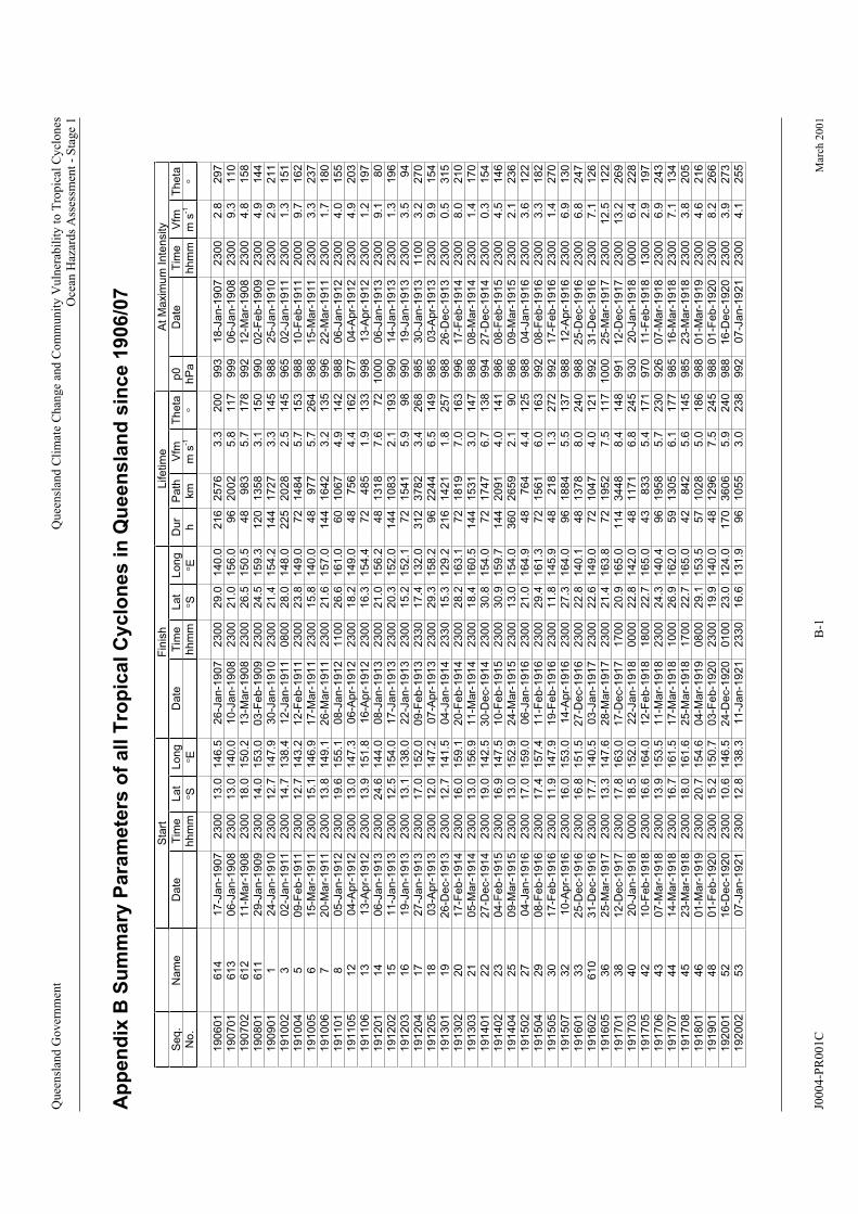
Quee
nsl
and G
over
nm
ent
Qu
een
slan
d C
lim
ate
Ch
ange
and
Co
mm
un
ity
Vuln
erab
ilit
y t
o T
rop
ical
Cy
clo
nes
Oce
an H
azar
ds
Ass
essm
ent
- S
tag
e 1
Ap
pe
nd
ix B
Su
mm
ary
Pa
ram
ete
rs o
f a
ll T
rop
ica
l C
yc
lon
es
in
Qu
ee
ns
lan
d s
inc
e 1
90
6/0
7
Sta
rtF
inis
hL
ife
tim
eA
t M
axim
um
In
ten
sity
Se
q.
Na
me
Da
teT
ime
La
tL
on
gD
ate
Tim
eL
at
Lo
ng
Du
rP
ath
Vfm
Th
eta
p0
Da
teT
ime
Vfm
Th
eta
No
.h
hm
mS
Eh
hm
mS
Eh
km
ms
-1h
Pa
hh
mm
ms
-1
19
06
01
61
41
7-J
an
-19
07
23
00
13
.01
46
.52
6-J
an
-19
07
23
00
29
.01
40
.02
16
25
76
3.3
20
09
93
18
-Ja
n-1
90
72
30
02
.82
97
19
07
01
61
30
6-J
an
-19
08
23
00
13
.01
40
.01
0-J
an
-19
08
23
00
21
.01
56
.09
62
00
25
.81
17
99
90
6-J
an
-19
08
23
00
9.3
11
0
19
07
02
61
21
1-M
ar-
19
08
23
00
18
.01
50
.21
3-M
ar-
19
08
23
00
26
.51
50
.54
89
83
5.7
17
89
92
12
-Ma
r-1
90
82
30
04
.81
58
19
08
01
61
12
9-J
an
-19
09
23
00
14
.01
53
.00
3-F
eb
-19
09
23
00
24
.51
59
.31
20
13
58
3.1
15
09
90
02
-Fe
b-1
90
92
30
04
.91
44
19
09
01
12
4-J
an
-19
10
23
00
12
.71
47
.93
0-J
an
-19
10
23
00
21
.41
54
.21
44
17
27
3.3
14
59
88
25
-Ja
n-1
91
02
30
02
.92
11
19
10
02
30
2-J
an
-19
11
23
00
14
.71
38
.41
2-J
an
-19
11
08
00
28
.01
48
.02
25
20
28
2.5
14
59
65
02
-Ja
n-1
91
12
30
01
.31
51
191004
509-F
eb
-1911
2300
12.7
143.2
12-F
eb
-1911
2300
23.8
149.0
72
1484
5.7
153
988
10-F
eb
-1911
2000
9.7
162
19
10
05
61
5-M
ar-
19
11
23
00
15
.11
46
.91
7-M
ar-
19
11
23
00
15
.81
40
.04
89
77
5.7
26
49
88
15
-Ma
r-1
91
12
30
03
.32
37
19
10
06
72
0-M
ar-
19
11
23
00
13
.81
49
.12
6-M
ar-
19
11
23
00
21
.61
57
.01
44
16
42
3.2
13
59
96
22
-Ma
r-1
91
12
30
01
.71
80
19
11
01
80
5-J
an
-19
12
23
00
19
.61
55
.10
8-J
an
-19
12
11
00
26
.61
61
.06
01
06
74
.91
42
98
80
6-J
an
-19
12
23
00
4.0
15
5
19
11
05
12
04
-Ap
r-1
91
22
30
01
3.0
14
7.3
06
-Ap
r-1
91
22
30
01
8.2
14
9.0
48
75
64
.41
62
97
70
4-A
pr-
19
12
23
00
4.9
20
3
19
11
06
13
13
-Ap
r-1
91
22
30
01
3.9
15
1.8
16
-Ap
r-1
91
22
30
01
6.3
15
4.4
72
48
51
.91
33
99
81
3-A
pr-
19
12
23
00
1.2
19
7
19
12
01
14
06
-Ja
n-1
91
32
30
02
4.6
14
4.0
08
-Ja
n-1
91
32
30
02
1.0
15
6.2
48
13
18
7.6
72
10
00
06
-Ja
n-1
91
32
30
09
.18
0
19
12
02
15
11
-Ja
n-1
91
32
30
01
2.5
15
4.0
17
-Ja
n-1
91
32
30
02
0.3
15
2.0
14
41
08
32
.11
93
99
01
4-J
an
-19
13
23
00
1.3
19
6
19
12
03
16
19
-Ja
n-1
91
32
30
01
3.1
13
8.0
22
-Ja
n-1
91
32
30
01
5.2
15
2.1
72
15
41
5.9
98
99
01
9-J
an
-19
13
23
00
3.5
94
19
12
04
17
27
-Ja
n-1
91
32
30
01
7.0
15
2.0
09
-Fe
b-1
91
32
33
01
7.4
13
2.0
31
23
78
23
.42
68
98
53
0-J
an
-19
13
11
00
3.2
27
0
19
12
05
18
03
-Ap
r-1
91
32
30
01
2.0
14
7.2
07
-Ap
r-1
91
32
30
02
9.3
15
8.2
96
22
44
6.5
14
99
85
03
-Ap
r-1
91
32
30
09
.91
54
19
13
01
19
26
-De
c-1
91
32
30
01
2.7
14
1.5
04
-Ja
n-1
91
42
33
01
5.3
12
9.2
21
61
42
11
.82
57
98
82
6-D
ec-1
91
32
30
00
.53
15
191302
20
17-F
eb
-1914
2300
16.0
159.1
20-F
eb
-1914
2300
28.2
163.1
72
1819
7.0
163
996
17-F
eb
-1914
2300
8.0
210
19
13
03
21
05
-Ma
r-1
91
42
30
01
3.0
15
6.9
11
-Ma
r-1
91
42
30
01
8.4
16
0.5
14
41
53
13
.01
47
98
80
8-M
ar-
19
14
23
00
1.4
17
0
19
14
01
22
27
-De
c-1
91
42
30
01
9.0
14
2.5
30
-De
c-1
91
42
30
03
0.8
15
4.0
72
17
47
6.7
13
89
94
27
-De
c-1
91
42
30
00
.31
54
19
14
02
23
04
-Fe
b-1
91
52
30
01
6.9
14
7.5
10
-Fe
b-1
91
52
30
03
0.9
15
9.7
14
42
09
14
.01
41
98
60
8-F
eb
-19
15
23
00
4.5
14
6
19
14
04
25
15
2.9
23
00
90
09
-Ma
r-1
91
52
30
01
3.0
24
-Ma
r-1
91
51
3.0
15
4.0
36
02
65
92
.19
86
09
-Ma
r-1
91
52
30
02
.12
36
19
15
02
27
15
9.0
23
00
04
-Ja
n-1
91
62
30
01
7.0
06
-Ja
n-1
91
62
1.0
16
4.9
48
76
44
.41
25
98
80
4-J
an
-19
16
23
00
3.6
12
2
19
15
04
29
23
00
08-F
eb
-1916
2300
17.4
157.4
11-F
eb
-1916
2300
29.4
161.3
72
1561
6.0
163
992
08-F
eb
-1916
3.3
182
30
23
00
11
.91
47
.91
9-F
eb
-19
16
23
00
11
.81
45
.94
82
18
1.3
27
29
92
17
-Fe
b-1
91
61
.42
70
32
10
-Ap
r-1
91
62
30
01
6.0
15
3.0
14
-Ap
r-1
91
62
30
02
7.3
16
4.0
96
18
84
5.5
13
79
88
12
-Ap
r-1
91
66
.9
19
16
01
33
25
-De
c-1
91
62
30
01
6.8
15
1.5
27
-De
c-1
91
62
30
02
2.8
14
0.1
48
13
78
8.0
24
09
88
25
-De
c-1
91
62
30
06
.82
47
19
16
02
61
03
1-D
ec-1
91
62
30
01
7.7
14
0.5
03
-Ja
n-1
91
72
30
02
2.6
14
9.0
72
10
47
4.0
12
19
92
31
-De
c-1
91
62
30
07
.11
26
19
16
05
36
25
-Ma
r-1
91
72
30
01
3.3
14
7.6
28
-Ma
r-1
91
72
30
02
1.4
16
3.8
72
19
52
7.5
11
71
00
02
5-M
ar-
19
17
23
00
12
.51
22
19
17
01
38
17
-De
c-1
91
71
2-D
ec-1
91
72
30
01
7.8
16
3.0
17
00
20
.91
65
.01
14
34
48
8.4
14
89
91
12
-De
c-1
91
72
30
01
3.2
26
9
19
17
03
40
20
-Ja
n-1
91
80
00
01
8.5
15
2.0
22
-Ja
n-1
91
80
00
02
2.8
14
2.0
48
11
71
6.8
24
59
30
20
-Ja
n-1
91
80
00
06
.42
28
191705
42
10-F
eb
-1918
2300
16.6
164.0
12-F
eb
-1918
1800
22.7
165.0
43
833
5.4
171
970
11-F
eb
-1918
1300
2.9
197
19
17
06
43
07
-Ma
r-1
91
82
30
01
3.9
15
3.5
11
-Ma
r-1
91
82
30
02
4.3
14
0.4
96
19
58
5.7
23
09
26
07
-Ma
r-1
91
82
30
06
.92
43
19
17
07
44
16
2.0
14-M
ar-
1918
2300
16.7
161.5
17-M
ar-
1918
1000
26.9
59
1305
6.1
177
985
16-M
ar-
1918
2300
7.1
134
19
17
08
45
23
-Ma
r-1
91
82
30
01
8.0
16
1.6
25
-Ma
r-1
91
81
70
02
2.7
16
5.0
42
84
25
.61
45
98
52
3-M
ar-
19
18
23
00
3.8
20
5
19
18
01
46
01
-Ma
r-1
91
92
30
02
0.7
15
4.6
04
-Ma
r-1
91
90
80
02
9.1
15
3.5
57
10
28
5.0
18
69
88
01
-Ma
r-1
91
92
30
04
.62
16
191901
48
01-F
eb
-1920
2300
15.2
150.7
03-F
eb
-1920
2300
19.9
140.0
48
1296
7.5
245
988
01-F
eb
-1920
2300
8.2
266
19
20
01
52
12
4.0
16
-De
c-1
92
02
30
01
0.6
14
6.5
24
-De
c-1
92
00
10
02
3.0
17
03
60
65
.92
40
98
81
6-D
ec-1
92
02
30
03
.92
73
19
20
02
53
07
-Ja
n-1
92
12
30
01
2.8
13
8.3
11
-Ja
n-1
92
12
33
01
6.6
13
1.9
96
10
55
3.0
23
89
92
07
-Ja
n-1
92
12
30
04
.12
55
191505
17-F
eb
-1916
23
00
19
15
07
23
00
13
0
J0004-P
R001C
B-1
Mar
ch 2
00
1
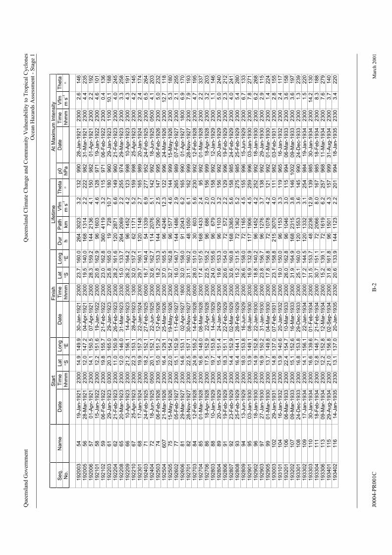
Quee
nsl
and G
over
nm
ent
Qu
een
slan
d C
lim
ate
Ch
ange
and
Co
mm
un
ity
Vuln
erab
ilit
y t
o T
rop
ical
Cy
clo
nes
Oce
an H
azar
ds
Ass
essm
ent
- S
tag
e 1
Sta
rtF
inis
hL
ife
tim
eA
t M
axim
um
In
ten
sity
Se
q.
Na
me
Da
teT
ime
La
tL
on
gD
ate
Tim
eL
at
Lo
ng
Du
rP
ath
Vfm
Th
eta
p0
Da
teT
ime
Vfm
Th
eta
No
.h
hm
mS
Eh
hm
mS
Eh
km
ms
-1h
Pa
hh
mm
ms
-1
19
20
03
54
14
.91
60
.02
.61
9-J
an
-19
21
23
00
14
9.9
30
-Ja
n-1
92
12
30
02
3.7
26
43
02
33
.21
32
99
02
8-J
an
-19
21
23
00
14
6
19
20
05
56
28
-Ma
r-1
92
12
30
01
2.0
14
7.2
04
-Ap
r-1
92
12
30
01
9.5
14
0.0
16
81
31
42
.22
22
98
23
1-M
ar-
19
21
23
00
4.4
23
5
19
20
06
57
15
9.2
01
-Ap
r-1
92
12
30
01
4.1
15
0.5
07
-Ap
r-1
92
12
30
02
8.3
14
42
13
64
.11
50
98
20
1-A
pr-
19
21
23
00
2.2
19
2
19
21
01
58
15
-Ja
n-1
92
22
30
01
2.2
15
1.6
19
-Ja
n-1
92
22
30
02
0.8
16
2.9
96
16
03
4.6
12
89
71
19
-Ja
n-1
92
22
30
04
.61
01
19
21
02
59
06
-Fe
b-1
92
22
30
01
9.8
15
5.7
21
-Fe
b-1
92
22
30
02
3.0
16
2.8
36
04
11
93
.21
15
97
10
6-F
eb
-19
22
23
00
0.4
13
6
19
22
03
61
29
-Ja
n-1
92
30
30
02
0.3
16
5.0
29
-Ja
n-1
92
32
20
02
5.8
16
5.0
19
72
81
0.7
18
09
60
29
-Ja
n-1
92
31
10
01
0.1
18
8
19
22
04
62
21
-Fe
b-1
92
32
30
01
1.0
15
0.9
26
-Fe
b-1
92
32
30
02
8.2
16
1.6
12
02
87
16
.61
49
96
02
1-F
eb
-19
23
23
00
4.0
24
5
19
22
08
65
20
-Ma
r-1
92
32
30
01
2.0
14
6.0
31
-Ma
r-1
92
32
33
01
5.0
13
3.7
26
42
06
92
.22
55
97
42
9-M
ar-
19
23
23
00
3.3
25
8
19
22
09
66
10
-Ap
r-1
92
32
30
02
1.2
15
6.1
14
-Ap
r-1
92
32
30
02
6.2
16
4.2
96
14
52
4.2
12
39
98
10
-Ap
r-1
92
32
30
04
.31
91
19
22
10
67
25
-Ap
r-1
92
32
30
02
2.3
15
3.1
28
-Ap
r-1
92
31
30
03
2.0
15
7.2
62
11
71
5.2
15
99
98
25
-Ap
r-1
92
32
30
04
.21
45
19
23
01
68
17
-Ja
n-1
92
42
30
01
9.9
15
7.3
22
-Ja
n-1
92
42
30
02
9.7
16
0.1
12
01
14
82
.71
65
98
92
0-J
an
-19
24
23
00
2.4
17
4
192403
71
24-F
eb
-1925
2300
18.2
152.1
27-F
eb
-1925
0500
16.7
140.4
54
1339
6.9
277
952
24-F
eb
-1925
2300
6.5
264
72
18
-Ju
n-1
92
50
50
02
0.1
15
2.1
22
-Ju
n-1
92
52
30
03
2.6
16
2.7
11
42
07
65
.11
42
99
21
8-J
un
-19
25
05
00
4.1
20
3
19
25
03
74
15
3.3
06-F
eb
-1926
2300
15.0
151.2
12-F
eb
-1926
2300
18.2
144
1290
2.5
147
995
06-F
eb
-1926
2300
5.0
232
19
25
04
60
72
1-M
ar-
19
26
23
00
16
.41
29
.12
5-M
ar-
19
26
23
00
37
.01
65
.59
64
24
61
2.3
12
29
96
24
-Ma
r-1
92
62
30
01
2.7
11
8
19
25
05
75
15
-Ma
y-1
92
62
30
02
2.0
15
4.2
19
-Ma
y-1
92
62
30
03
2.7
16
2.8
96
15
77
4.6
14
49
99
15
-Ma
y-1
92
62
30
05
.31
80
19
26
02
77
15
2.9
14
0.7
05-F
eb
-1927
2300
15.1
11-F
eb
-1927
2300
16.0
144
1486
2.9
265
989
07-F
eb
-1927
2300
2.1
255
19
26
06
81
29
-Ma
r-1
92
72
30
01
4.6
15
3.1
02
-Ap
r-1
92
71
80
03
2.0
15
8.0
91
20
43
6.2
16
59
90
01
-Ap
r-1
92
71
80
06
.91
70
19
27
01
82
28
-No
v-1
92
72
30
02
2.5
15
7.1
30
-No
v-1
92
72
30
03
1.1
16
0.2
48
10
50
6.1
16
29
99
28
-No
v-1
92
72
30
07
.91
93
192703
84
12-F
eb
-1928
23
00
23
00
24
.91
55
.21
4-F
eb
-19
28
05
00
28
.01
51
.03
06
03
5.6
23
09
92
12
-Fe
b-1
92
84
.71
95
19
27
04
85
17
.49
92
23
00
01
-Ma
r-1
92
82
30
01
6.6
14
8.0
08
-Ma
r-1
92
82
30
01
57
.51
68
14
33
2.4
95
01
-Ma
r-1
92
82
.23
37
19
27
06
86
18
-Ap
r-1
92
82
30
01
7.5
15
2.9
22
-Ap
r-1
92
82
30
02
2.5
15
5.2
96
68
62
.01
56
99
91
8-A
pr-
19
28
23
00
3.2
20
3
19
28
03
88
10
-Ja
n-1
92
92
30
01
9.7
15
3.8
14
-Ja
n-1
92
92
30
02
4.0
15
5.6
96
67
92
.01
58
99
21
2-J
an
-19
29
23
00
1.1
14
6
19
28
04
89
20
-Ja
n-1
92
92
30
01
5.4
15
1.4
24
-Ja
n-1
92
92
30
01
9.6
15
3.3
96
11
03
3.2
15
69
92
20
-Ja
n-1
92
92
30
05
.02
40
192806
91
19-F
eb
-1929
2300
18.3
151.1
22-F
eb
-1929
2300
20.6
154.0
72
572
2.2
129
996
19-F
eb
-1929
2300
2.3
212
192807
92
23-F
eb
-1929
2300
14.4
152.9
02-M
ar-
1929
2300
32.6
160.8
168
3365
5.6
158
985
24-F
eb
-1929
2300
4.0
241
192808
93
28-F
eb
-1929
25
-Fe
b-1
92
92
30
01
6.4
14
4.1
23
30
15
.21
31
.57
21
36
25
.22
75
98
52
5-F
eb
-19
29
23
00
5.4
28
0
19
28
09
94
13
-Ju
n-1
92
92
30
01
8.0
15
3.8
16
-Ju
n-1
92
92
30
02
6.6
15
8.0
72
11
65
4.5
15
59
96
15
-Ju
n-1
92
92
30
06
.71
33
19
29
01
95
03
-Ja
n-1
93
02
30
01
3.9
14
9.1
08
-Ja
n-1
93
02
03
01
6.9
13
2.9
11
71
90
64
.52
59
99
60
3-J
an
-19
30
23
00
7.8
27
1
19
29
02
96
14
0.2
18
-Ja
n-1
93
06
.21
8-J
an
-19
30
23
00
14
.91
52
.82
2-J
an
-19
30
23
00
18
.89
61
45
24
.22
52
99
22
30
02
68
19
29
03
97
15
6.7
29
-Ja
n-1
93
02
.92
7-J
an
-19
30
23
00
16
.91
50
.23
1-J
an
-19
30
23
00
23
.89
61
27
63
.71
38
99
22
30
01
15
19
29
05
99
01-M
ar-
1930
01
-Ma
r-1
93
02
30
01
3.7
14
9.8
04
-Ma
r-1
93
02
30
01
7.8
15
6.8
72
10
78
4.2
12
19
92
23
00
1.4
22
4
19
30
03
10
21
11
29
-Ja
n-1
93
12
33
01
4.8
13
7.0
07
-Fe
b-1
93
12
30
02
3.1
15
8.8
21
53
07
04
.09
82
03
-Fe
b-1
93
12
30
02
.81
55
19
31
01
10
41
6-J
an
-19
32
23
00
13
.91
40
.62
0-J
an
-19
32
23
00
19
.01
50
.09
61
15
33
.31
19
96
51
6-J
an
-19
32
23
00
2.4
11
7
19
32
01
10
60
6-M
ar-
19
33
23
00
22
.41
54
.71
0-M
ar-
19
33
23
00
26
.01
62
.89
61
04
63
.01
15
99
40
6-M
ar-
19
33
23
00
3.6
15
8
19
32
02
10
70
9-M
ar-
19
33
23
00
15
.11
52
.61
6-M
ar-
19
33
23
00
31
.91
64
.91
68
23
15
3.8
14
61
00
20
9-M
ar-
19
33
23
00
3.6
19
7
19
33
01
10
82
4-D
ec-1
93
32
30
01
6.8
15
3.8
29
-De
c-1
93
32
30
02
5.1
16
0.0
12
01
55
33
.61
45
99
02
4-D
ec-1
93
32
30
01
.32
39
19
33
02
10
91
7-J
an
-19
34
23
00
14
.11
56
.12
2-J
an
-19
34
23
00
17
.21
44
.51
20
13
32
3.1
25
49
84
19
-Ja
n-1
93
42
30
01
.52
20
19
33
03
11
03
0-J
an
-19
34
23
00
16
.61
39
.60
1-F
eb
-19
34
23
00
31
.51
53
.74
82
23
61
2.9
13
99
85
30
-Ja
n-1
93
42
30
01
4.2
13
0
19
33
04
11
11
8-F
eb
-19
34
23
00
12
.81
46
.72
1-F
eb
-19
34
23
00
30
.71
51
.17
22
06
68
.01
67
98
51
8-F
eb
-19
34
23
00
8.3
18
8
19
33
06
11
30
9-M
ar-
19
34
23
00
12
.21
52
.81
2-M
ar-
19
34
23
00
15
.21
39
.17
21
61
96
.22
57
96
81
1-M
ar-
19
34
23
00
7.6
27
9
19
34
01
11
52
9-A
ug
-19
34
23
00
21
.01
56
.80
2-S
ep
-19
34
23
00
31
.81
61
.89
61
50
14
.31
57
99
93
1-A
ug
-19
34
23
00
3.7
14
0
20
.6
19
24
04
19
34
02
11
61
4-J
an
-19
35
23
30
13
.11
37
.02
0-J
an
-19
35
23
30
13
3.9
14
41
12
32
.22
01
99
41
8-J
an
-19
35
23
30
3.4
22
0
J0004-P
R001C
B-2
Mar
ch 2
00
1
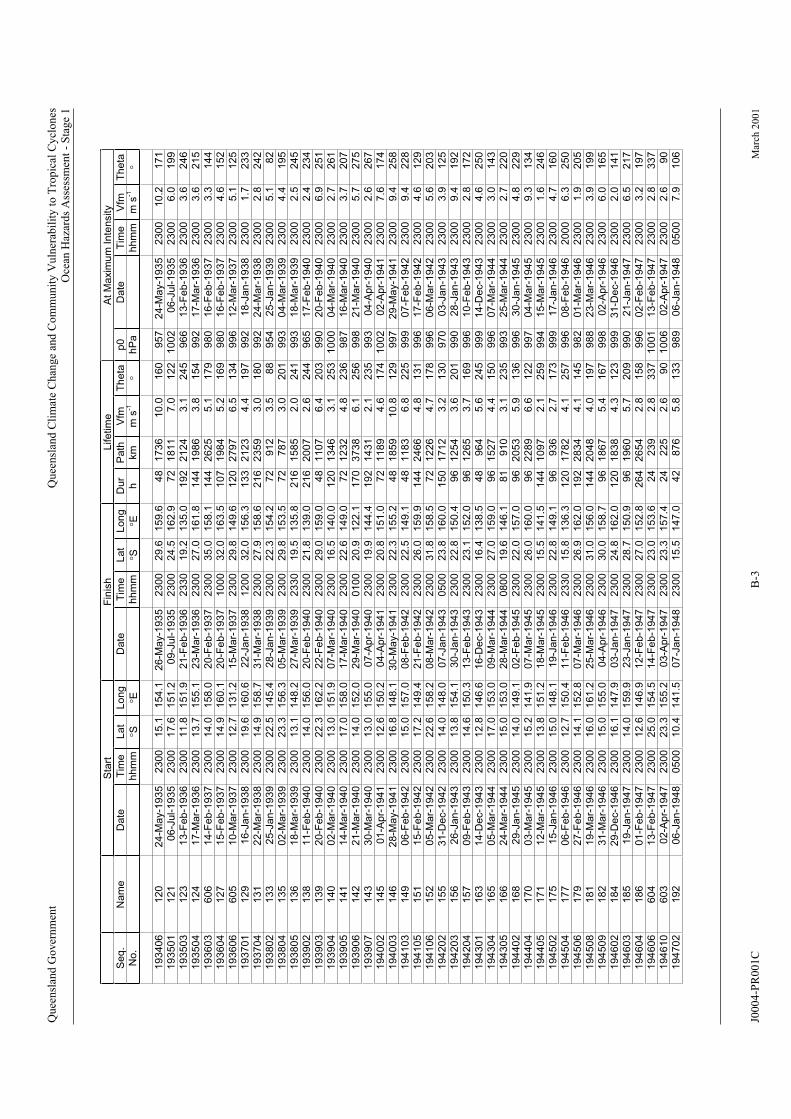
Quee
nsl
and G
over
nm
ent
Qu
een
slan
d C
lim
ate
Ch
ange
and
Co
mm
un
ity
Vuln
erab
ilit
y t
o T
rop
ical
Cy
clo
nes
Oce
an H
azar
ds
Ass
essm
ent
- S
tag
e 1
Sta
rtF
inis
hL
ife
tim
eA
t M
axim
um
In
ten
sity
Se
q.
Da
teT
ime
La
tL
on
gD
ate
Tim
eL
at
Lo
ng
Du
rP
ath
Vfm
Th
eta
p0
Da
teT
ime
Vfm
Th
eta
No
.h
hm
mS
Eh
hm
mS
Eh
km
ms
-1h
Pa
hh
mm
ms
-1
5.4
167
998
02-A
pr-
1946
2300
6.0
165
19
46
02
18
42
9-D
ec-1
94
62
30
01
6.1
14
7.9
03
-Ja
n-1
94
72
30
02
4.8
16
2.0
12
01
83
84
.31
23
99
93
1-D
ec-1
94
62
30
02
.01
41
19
46
03
18
52
30
01
4.0
15
9.9
23
-Ja
n-1
94
72
30
02
8.7
15
0.9
96
19
60
5.7
20
99
90
21
-Ja
n-1
94
72
30
06
.52
17
19
46
04
18
60
1-F
eb
-19
47
23
00
12
.61
46
.91
2-F
eb
-19
47
23
00
27
.01
52
.82
64
26
54
2.8
15
89
96
02
-Fe
b-1
94
72
30
03
.21
97
19
46
06
60
41
3-F
eb
-19
47
23
00
25
.01
54
.51
4-F
eb
-19
47
23
00
23
.01
53
.62
42
39
2.8
33
71
00
11
3-F
eb
-19
47
23
00
2.8
33
7
19
46
10
60
30
2-A
pr-
19
47
23
00
23
.31
55
.20
3-A
pr-
19
47
23
00
23
.31
57
.42
42
25
2.6
90
10
06
02
-Ap
r-1
94
72
30
02
.69
0
19
47
02
19
20
6-J
an
-19
48
05
00
10
.41
41
.50
7-J
an
-19
48
23
00
15
.51
47
.04
28
76
5.8
13
39
89
06
-Ja
n-1
94
80
50
07
.91
06
Na
me
19
34
06
12
01
54
.11
71
24
-Ma
y-1
93
52
30
01
5.1
26
-Ma
y-1
93
52
30
02
9.6
15
9.6
48
17
36
10
.01
60
95
72
4-M
ay-1
93
5
06
-Ju
l-1
93
5
23
00
10
.2
19
35
01
12
10
6-J
ul-1
93
52
30
01
7.6
15
1.2
09
-Ju
l-1
93
52
30
02
4.5
16
2.9
72
18
11
21
24
7.0
12
21
00
22
30
06
.0
3.6
19
9
193503
123
13-F
eb
-1936
2300
11.8
151.9
21-F
eb
-1936
23-M
ar-
1936
23
30
19
.21
35
.0
16
1.8
192
3.1
245
966
13-F
eb
-1936
17-M
ar-
1936
23
00
24
6
19
35
04
12
41
98
61
7-M
ar-
19
36
23
00
13
.71
55
.1
15
8.0
23
00
27
.01
44
3.8
15
49
92
23
00
3.6
21
5
193603
606
14-F
eb
-1937
2300
14.0
20-F
eb
-1937
2300
35.0
158.1
144
2625
5.1
179
980
16-F
eb
-1937
16-F
eb
-1937
23
00
3.3
14
4
19
36
04
12
71
5-F
eb
-19
37
23
00
14
.91
60
.12
0-F
eb
-19
37
10
00
32
.01
63
.51
07
19
84
5.2
16
99
80
23
00
4.6
15
2
19
36
06
19
37
01
60
51
0-M
ar-
19
37
23
00
12
.71
31
.21
5-M
ar-
19
37
23
00
29
.81
49
.61
20
27
97
6.5
13
49
96
12
-Ma
r-1
93
72
30
05
.1
1.7
12
5
12
91
6-J
an
-19
38
23
00
19
.61
60
.6
15
8.7
22
-Ja
n-1
93
81
20
03
2.0
15
6.3
15
8.6
13
32
12
34
.41
97
99
21
8-J
an
-19
38
23
00
23
00
23
3
19
37
04
13
1
13
3
22-M
ar-
1938
2300
23
00
14.9
31-M
ar-
1938
2300
27.9
22
.3
21
62
35
93
.01
80
88
992
24-M
ar-
1938
2.8
242
19
38
02
25
-Ja
n-1
93
92
2.5
14
5.4
15
6.3
28
-Ja
n-1
93
92
30
01
54
.27
29
12
78
7
3.5
95
42
5-J
an
-19
39
23
00
5.1
82
19
38
04
13
50
2-M
ar-
19
39
23
00
23
.30
5-M
ar-
19
39
23
00
29
.81
53
.57
23
.02
01
99
30
4-M
ar-
19
39
23
00
4.4
19
5
19
38
05
19
39
02
13
61
8-M
ar-
19
39
11-F
eb
-1940
23
00
13
.11
48
.22
7-M
ar-
19
39
23
30
19
.51
35
.82
16
15
85
2.0
24
19
93
18
-Ma
r-1
93
92
30
02
.52
45
138
2300
14.0
156.0
20-F
eb
-1940
2300
23
00
21
.81
39
.0
15
9.0
216
2007
2.6
244
965
17-F
eb
-1940
2300
2.4
6.9
23
4
193903
139
20-F
eb
-1940
02-M
ar-
1940
23
00
22
.3
13
.0
162.2
22-F
eb
-1940
29.0
48
1107
6.4
203
990
20-F
eb
-1940
2300
251
19
39
04
14
01
40
.02300
151.9
07-M
ar-
1940
2300
16.5
120
1346
3.1
253
1000
04-M
ar-
1940
2300
2.7
261
19
39
05
14
11
4-M
ar-
19
40
23
00
17
.0
14
.0
158.0
17-M
ar-
1940
29-M
ar-
1940
23
00
22
.61
49
.07
21
23
24
.8
6.1
236
987
16-M
ar-
1940
2300
3.7
207
19
39
06
14
2
14
3
21
-Ma
r-1
94
02
30
01
52
.00
10
02
0.9
12
2.1
17
03
73
82
56
99
82
1-M
ar-
19
40
04-A
pr-
1940
23
00
5.7
27
5
19
39
07
30
-Ma
r-1
94
02
30
01
3.0
15
5.0
07
-Ap
r-1
94
02
30
01
9.9
14
4.4
19
21
43
12
.12
35
99
32
30
02
.62
67
19
40
02
14
50
1-A
pr-
19
41
23
00
12
.61
50
.20
4-A
pr-
19
41
23
00
20
.81
51
.07
21
18
94
.61
74
10
02
02
-Ap
r-1
94
12
30
07
.61
74
19
40
03
14
62
8-M
ay-1
94
12
30
0
23
00
16
.81
48
.1
15
7.0
30
-Ma
y-1
94
12
30
0
23
00
22
.31
55
.2
14
9.1
48
18
59
11
83
10
.81
29
22
5
99
72
9-M
ay-1
94
12
30
09
.4
9.4
25
8
194103
149
06-F
eb
-1942
15.0
08-F
eb
-1942
22.5
48
6.8
999
07-F
eb
-1942
2300
228
19
41
05
15
1
15
2
14
9.4
15-F
eb
-1942
2300
17.2
21-F
eb
-1942
2300
26.0
159.9
15
8.5
144
2466
4.8
131
996
17-F
eb
-1942
2300
4.6
5.6
12
9
19
41
06
05
-Ma
r-1
94
22
30
0
23
00
22
.61
58
.20
8-M
ar-
19
42
23
00
31
.87
21
22
64
.71
78
99
6
97
0
06-M
ar-
1942
2300
23
00
20
3
12
51
94
20
2
19
42
03
15
53
1-D
ec-1
94
2
26
-Ja
n-1
94
3
14
.0
13
.8
14
8.0
07
-Ja
n-1
94
3
30
-Ja
n-1
94
3
05
00
23
.8
22
.8
16
0.0
15
01
71
23
.21
30
03
-Ja
n-1
94
33
.9
15
62
30
01
54
.12
30
01
50
.49
61
25
43
.62
01
99
02
8-J
an
-19
43
23
00
9.4
19
2
19
42
04
15
70
9-F
eb
-19
43
23
00
14
.61
50
.31
3-F
eb
-19
43
23
00
23
.11
52
.09
61
26
53
.71
69
99
61
0-F
eb
-19
43
23
00
2.8
17
2
19
43
01
16
31
4-D
ec-1
94
32
30
01
2.8
14
6.6
16
-De
c-1
94
32
30
01
6.4
13
8.5
48
96
4
15
27
5.6
24
5
15
0
99
91
4-D
ec-1
94
3
07-M
ar-
1944
23
00
4.6
3.0
25
0
19
43
04
16
50
5-M
ar-
19
44
23
00
17
.01
53
.00
9-M
ar-
19
44
23
00
27
.01
59
.09
64
.49
96
23
00
14
3
19
43
05
16
62
4-M
ar-
19
44
23
00
15
.01
53
.02
8-M
ar-
19
44
08
00
19
.61
46
.18
19
10
3.1
23
59
93
25
-Ma
r-1
94
42
30
02
.72
20
19
44
02
16
82
9-J
an
-19
45
23
00
23
00
14.0
149.1
02-F
eb
-1945
2300
22.0
26
.0
15
7.0
96
20
53
5.9
13
69
96
30
-Ja
n-1
94
5
04-M
ar-
1945
23
00
4.8
22
9
19
44
04
17
0
17
1
03
-Ma
r-1
94
51
5.2
14
1.9
07
-Ma
r-1
94
52
30
01
60
.09
62
28
9
10
97
6.6
12
29
97
23
00
9.3
13
4
19
44
05
23
00
12-M
ar-
1945
13.8
151.2
18-M
ar-
1945
2300
23
00
15
.51
41
.51
44
2.1
25
99
94
15
-Ma
r-1
94
52
30
01
.6
4.7
24
6
19
45
02
19
45
04
17
51
5-J
an
-19
46
23
00
23
00
15
.01
48
.11
9-J
an
-19
46
22
.81
49
.1
13
6.3
96
93
62
.71
73
99
91
7-J
an
-19
46
23
00
16
0
25
0177
06-F
eb
-1946
12.7
150.4
11-F
eb
-1946
2330
15.8
120
1782
4.1
257
14
5
996
08-F
eb
-1946
01-M
ar-
1946
20
00
6.3
19
45
06
17
92
7-F
eb
-19
46
23
00
14
.11
52
.80
7-M
ar-
19
46
23
00
26
.91
62
.01
92
28
34
4.1
98
22
30
01
.92
05
19
45
08
18
11
97
19
-Ma
r-1
94
62
30
01
6.0
16
1.2
25
-Ma
r-1
94
62
30
03
1.0
15
6.0
14
42
04
84
.09
88
23
-Ma
r-1
94
62
30
03
.91
99
19
45
09
18
23
1-M
ar-
19
46
23
00
15
.01
55
.00
4-A
pr-
19
46
23
00
30
.01
58
.79
61
86
7
19
-Ja
n-1
94
7
J0004-P
R001C
B-3
Mar
ch 2
00
1

Quee
nsl
and G
over
nm
ent
Qu
een
slan
d C
lim
ate
Ch
ange
and
Co
mm
un
ity
Vuln
erab
ilit
y t
o T
rop
ical
Cy
clo
nes
Oce
an H
azar
ds
Ass
essm
ent
- S
tag
e 1
Sta
rtF
inis
hL
ife
tim
eA
t M
axim
um
In
ten
sity
Se
q.
Da
teT
ime
La
tL
on
gD
ate
Tim
eL
at
Lo
ng
Du
rP
ath
Vfm
Th
eta
p0
Da
teT
ime
Vfm
Th
eta
No
.h
hm
mS
Eh
hm
mS
Eh
km
ms
-1h
Pa
hh
mm
ms
-1
19
47
03
19
31
0-J
an
-19
48
23
00
15
.01
40
.01
5-J
an
-19
48
23
00
24
.01
61
.01
20
26
69
6.2
11
49
95
11
-Ja
n-1
94
82
30
03
.91
36
19
47
05
19
51
9-F
eb
-19
48
23
30
12
.81
34
.32
4-F
eb
-19
48
23
30
23
.11
34
.01
20
16
27
3.8
18
19
96
22
-Fe
b-1
94
82
33
04
.31
87
19
47
07
19
71
9-M
ar-
19
48
23
00
10
.71
56
.12
5-M
ar-
19
48
23
00
28
.01
61
.01
44
24
57
4.7
16
49
90
24
-Ma
r-1
94
82
30
07
.41
11
19
47
09
19
92
9-A
pr-
19
48
23
00
22
.81
53
.10
1-M
ay-1
94
82
30
02
4.9
15
0.0
48
41
92
.42
33
10
02
30
-Ap
r-1
94
82
30
02
.42
54
19
48
03
20
10
8-J
an
-19
49
23
00
13
.61
42
.01
2-J
an
-19
49
23
00
23
.51
62
.09
62
38
76
.91
17
99
21
0-J
an
-19
49
23
00
8.5
11
1
19
48
05
20
30
7-F
eb
-19
49
23
00
14
.01
52
.01
6-F
eb
-19
49
23
00
30
.21
63
.82
16
44
68
5.7
14
59
94
09
-Fe
b-1
94
92
30
02
.13
03
194807
205
25-F
eb
-1949
2300
14.0
156.0
02-M
ar-
1949
2300
23.1
149.1
120
1957
4.5
215
972
02-M
ar-
1949
0500
2.6
285
19
49
01
20
71
2-J
an
-19
50
23
00
14
.01
46
.91
6-J
an
-19
50
23
00
22
.31
52
.59
61
32
13
.81
47
99
41
4-J
an
-19
50
06
00
1.7
16
7
19
49
02
20
81
3-J
an
-19
50
23
00
16
.01
39
.01
8-J
an
-19
50
11
00
28
.01
50
.01
08
17
66
4.5
13
99
88
16
-Ja
n-1
95
02
30
05
.11
41
19
49
04
21
02
2-F
eb
-19
50
23
00
15
.61
53
.32
7-F
eb
-19
50
11
00
24
.61
51
.51
08
13
83
3.6
19
09
98
24
-Fe
b-1
95
02
30
02
.72
44
19
49
06
21
20
4-M
ar-
19
50
23
00
13
.01
46
.41
1-M
ar-
19
50
23
00
22
.91
44
.11
68
31
58
5.2
19
29
92
10
-Ma
r-1
95
02
30
06
.22
56
19
50
02
60
20
8-J
an
-19
51
23
00
16
.21
40
.02
3-J
an
-19
51
23
00
21
.91
43
.03
60
37
69
2.9
15
39
95
09
-Ja
n-1
95
12
30
05
.11
51
19
50
03
21
41
8-J
an
-19
51
23
00
16
.41
39
.72
2-J
an
-19
51
23
00
19
.11
40
.39
63
67
1.1
16
89
95
20
-Ja
n-1
95
12
30
02
.01
80
19
50
04
21
52
4-J
an
-19
51
23
00
24
.71
51
.72
9-J
an
-19
51
23
00
26
.01
50
.91
20
11
73
2.7
20
99
99
25
-Ja
n-1
95
12
30
02
.23
1
19
50
10
21
90
9-M
ar-
19
51
23
00
12
.51
45
.51
8-M
ar-
19
51
23
00
26
.21
51
.62
16
32
87
4.2
15
79
96
16
-Ma
r-1
95
12
30
06
.52
39
19
50
11
22
02
3-M
ar-
19
51
23
00
7.4
15
8.8
31
-Ma
r-1
95
12
30
02
3.6
16
2.7
19
22
59
13
.71
66
99
43
1-M
ar-
19
51
23
00
7.9
13
3
19
51
02
22
21
8-J
an
-19
52
23
30
11
.41
39
.42
1-J
an
-19
52
23
00
18
.21
39
.27
11
07
54
.21
81
99
41
9-J
an
-19
52
23
00
2.8
18
5
19
51
06
22
51
5-A
pr-
19
52
23
00
9.1
15
5.5
21
-Ap
r-1
95
22
30
02
5.0
16
5.0
14
42
57
75
.01
50
94
01
8-A
pr-
19
52
08
00
1.8
15
3
19
52
01
22
62
6-O
ct-
19
52
20
00
15
.71
50
.02
8-O
ct-
19
52
23
00
22
.91
60
.95
11
49
88
.21
24
99
82
6-O
ct-
19
52
20
00
11
.41
70
19
52
02
22
71
5-D
ec-1
95
21
10
01
7.4
15
8.3
16
-De
c-1
95
22
30
02
3.6
15
9.0
36
12
05
9.3
17
39
98
16
-De
c-1
95
22
30
01
2.2
11
0
19
52
04
22
81
2-J
an
-19
53
23
00
15
.41
39
.61
4-J
an
-19
53
23
30
18
.81
37
.64
84
55
2.6
20
99
95
13
-Ja
n-1
95
32
00
09
.62
10
19
52
06
22
91
58
.72
30
01
90
19-F
eb
-1953
0500
17.4
22-F
eb
-1953
26.0
157.0
90
1141
3.5
1002
19-F
eb
-1953
0500
5.2
211
19
52
08
23
11
53
.02
00
021-M
ar-
1953
2300
23.2
22-M
ar-
1953
25.0
151.2
21
295
3.9
222
1004
21-M
ar-
1953
2300
4.5
250
19
52
09
23
22
00
01
4-A
pr-
19
53
20
00
10
.41
42
.61
5-A
pr-
19
53
23
30
10
.91
38
.22
74
98
52
63
10
03
14
-Ap
r-1
95
31
2.7
24
1
23
42
30
01
3.0
14
2.0
07
-Ja
n-1
95
42
30
03
0.3
15
9.4
12
03
18
07
.41
36
99
60
3-J
an
-19
54
9.1
11
9
235
04-F
eb
-1954
2300
14.0
149.0
08-F
eb
-1954
1100
22.6
148.7
84
1046
3.5
181
990
07-F
eb
-1954
1.1
195303
236
16-F
eb
-1954
0200
16.0
165.0
20-F
eb
-1954
2300
29.1
152.4
117
2190
5.2
221
980
19-F
eb
-1954
1100
2.4
222
19
54
01
23
81
9-D
ec-1
95
42
30
01
2.2
15
5.0
22
-De
c-1
95
41
10
01
7.0
16
2.0
60
92
44
.31
25
10
00
22
-De
c-1
95
41
10
05
.61
17
19
54
03
60
13
0-D
ec-1
95
42
30
01
2.7
16
0.1
11
-Ja
n-1
95
52
30
02
4.6
17
1.2
28
83
15
83
13
81
00
23
0-D
ec-1
95
42
30
00
.98
1
195407
600
18-M
ar-
1955
01
-Ma
r-1
95
52
30
01
7.9
16
9.0
23
00
23
.51
38
.64
08
57
60
3.9
25
89
68
06
-Ma
r-1
95
52
30
04
.92
61
19
54
08
24
42
1-M
ar-
19
55
23
00
11
.01
64
.00
5-A
pr-
19
55
23
00
30
.01
57
.63
60
55
25
4.3
19
79
85
26
-Ma
r-1
95
52
30
04
.52
26
19
55
02
59
90
6-D
ec-1
95
52
30
02
0.4
16
6.5
16
-De
c-1
95
50
50
03
8.0
16
6.0
22
24
28
45
.41
81
10
01
10
-De
c-1
95
50
50
04
.82
54
19
55
04
24
72
6-D
ec-1
95
50
50
01
7.0
16
0.0
27
-De
c-1
95
51
10
02
0.0
16
4.5
30
63
05
.81
25
99
32
7-D
ec-1
95
50
50
06
.98
1
19
55
05
24
81
5-J
an
-19
56
23
00
15
.01
40
.02
7-J
an
-19
56
23
00
29
.91
60
.22
88
47
77
4.6
12
89
68
25
-Ja
n-1
95
62
30
07
.21
39
19
55
10
63
00
6-F
eb
-19
56
05
00
15
.01
49
.51
2-F
eb
-19
56
11
00
46
.21
66
.51
50
46
18
8.6
15
49
94
10
-Fe
b-1
95
61
10
04
.51
80
19
55
11
62
91
4-F
eb
-19
56
05
00
14
.01
46
.51
8-F
eb
-19
56
23
00
32
.51
51
.21
14
26
83
6.5
16
69
90
18
-Fe
b-1
95
60
20
03
.51
94
19
55
13
AG
NE
S2
3-F
eb
-19
56
05
00
17
.01
75
.01
1-M
ar-
19
56
23
00
29
.51
41
.24
26
56
76
3.7
24
89
61
06
-Ma
r-1
95
60
50
05
.73
09
19
55
15
25
41
4-M
ar-
19
56
23
00
24
.61
65
.31
6-M
ar-
19
56
23
00
29
.21
57
.24
81
07
66
.22
37
99
81
6-M
ar-
19
56
23
00
4.7
17
1
19
55
17
59
50
2-A
pr-
19
56
11
00
14
.01
54
.00
8-A
pr-
19
56
17
00
42
.01
73
.51
50
44
14
8.2
14
89
98
04
-Ap
r-1
95
60
50
09
.11
15
19
56
03
25
81
1-N
ov-1
95
61
10
01
2.0
15
6.5
14
-No
v-1
95
60
50
01
5.0
16
3.0
66
82
83
.51
15
10
02
11
-No
v-1
95
62
30
04
.31
35
19
56
05
PR
IMA
RY
18
-De
c-1
95
60
50
01
5.0
13
4.5
21
-De
c-1
95
60
80
01
8.0
14
1.3
75
88
13
.31
14
98
22
1-D
ec-1
95
60
50
04
.41
17
19
56
06
25
91
9-D
ec-1
95
61
40
01
5.1
13
6.9
21
-De
c-1
95
62
30
02
0.0
14
6.1
57
11
69
5.7
11
99
82
21
-De
c-1
95
60
50
06
.71
17
19
56
07
SE
CO
ND
AR
Y2
1-D
ec-1
95
62
00
02
6.3
15
3.5
23
-De
c-1
95
60
50
02
2.3
15
6.0
33
26
03
21
.92
99
98
22
-De
c-1
95
60
50
07
.73
38
Na
me
19
53
01
02
-Ja
n-1
95
42
30
0
19
53
02
08
00
21
2
J0004-P
R001C
B-4
Mar
ch 2
00
1
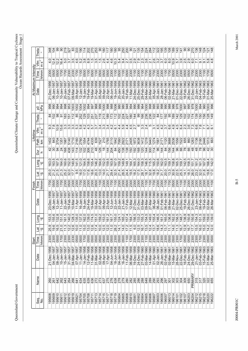
Quee
nsl
and G
over
nm
ent
Qu
een
slan
d C
lim
ate
Ch
ange
and
Co
mm
un
ity
Vuln
erab
ilit
y t
o T
rop
ical
Cy
clo
nes
Oce
an H
azar
ds
Ass
essm
ent
- S
tag
e 1
Sta
rtF
inis
hL
ife
tim
eA
t M
axim
um
In
ten
sity
Se
q.
Da
teT
ime
La
tL
on
gD
ate
Tim
eL
at
Lo
ng
Du
rP
ath
Vfm
Th
eta
p0
Da
teT
ime
Vfm
Th
eta
No
.h
hm
mS
Eh
hm
mS
Eh
km
ms
-1h
Pa
hh
mm
ms
-1
19
56
08
20
62
1-D
ec-1
95
62
30
02
5.9
15
3.5
23
-De
c-1
95
61
70
02
5.0
16
3.0
42
14
02
9.3
84
99
82
1-D
ec-1
95
62
30
04
.03
48
19
56
09
26
10
4-J
an
-19
57
23
00
19
.61
55
.60
6-J
an
-19
57
05
00
21
.21
63
.53
08
43
7.8
10
29
90
06
-Ja
n-1
95
70
50
01
2.4
10
4
19
56
10
64
20
8-J
an
-19
57
05
00
16
.51
32
.81
2-J
an
-19
57
03
00
21
.51
67
.59
43
70
41
0.9
98
99
41
0-J
an
-19
57
05
00
12
.29
9
19
56
11
26
21
0-J
an
-19
57
17
00
21
.01
51
.01
1-J
an
-19
57
17
00
21
.31
64
.02
41
35
11
5.6
91
99
41
0-J
an
-19
57
17
00
16
.49
0
19
56
12
64
31
5-J
an
-19
57
23
00
11
.31
61
.52
2-J
an
-19
57
23
00
25
.21
60
.61
68
19
87
3.3
18
39
98
20
-Ja
n-1
95
71
70
05
.02
19
19
56
15
26
43
1-J
an
-19
57
23
00
12
.21
40
.21
9-F
eb
-19
57
05
00
32
.01
52
.04
38
51
40
3.3
15
19
53
07
-Fe
b-1
95
72
30
03
.73
27
19
56
19
26
60
4-M
ar-
19
57
23
30
12
.61
28
.31
0-M
ar-
19
57
23
00
17
.71
40
.81
43
17
10
3.3
11
21
00
30
9-M
ar-
19
57
23
30
3.5
83
19
56
21
64
10
7-A
pr-
19
57
05
00
10
.01
35
.01
1-A
pr-
19
57
23
00
9.5
14
1.5
11
42
16
05
.38
51
00
20
9-A
pr-
19
57
17
00
4.6
33
3
63
41
1-J
an
-19
58
05
00
11
.01
37
.01
6-J
an
-19
58
17
00
16
.01
21
.01
32
27
60
5.8
25
21
00
41
2-J
an
-19
58
11
00
5.2
19
0
19
57
05
63
51
4-J
an
-19
58
17
00
15
.01
62
.01
8-J
an
-19
58
23
00
17
.01
64
.51
02
15
54
4.2
12
91
00
21
8-J
an
-19
58
05
00
3.8
11
4
195708
639
12-F
eb
-1958
0500
13.0
139.0
24-F
eb
-1958
2300
17.6
158.6
306
4744
4.3
103
994
19-F
eb
-1958
1100
8.9
202
19
57
11
63
61
1-M
ar-
19
58
05
00
12
.61
74
.51
9-M
ar-
19
58
23
00
18
.61
55
.42
10
43
35
5.7
25
19
97
19
-Ma
r-1
95
80
50
01
.52
70
19
57
13
27
21
51
.03
1-M
ar-
19
58
05
00
17
.40
2-A
pr-
19
58
05
00
20
.31
46
.24
86
39
3.7
23
79
68
01
-Ap
r-1
95
81
10
03
.52
53
19
57
14
27
30
2-A
pr-
19
58
05
00
10
.01
59
.20
7-A
pr-
19
58
11
00
13
.01
64
.61
26
15
27
3.4
11
99
99
05
-Ap
r-1
95
80
50
01
.59
0
19
57
15
63
70
9-A
pr-
19
58
05
00
12
.51
53
.00
9-A
pr-
19
58
23
00
14
.01
52
.01
82
10
3.3
21
31
00
00
9-A
pr-
19
58
05
00
2.6
18
0
19
57
17
27
51
7-A
pr-
19
58
05
00
23
00
12
.01
61
.22
3-A
pr-
19
58
23
00
21
.71
59
.51
44
17
65
3.4
18
99
98
22
-Ap
r-1
95
84
.41
17
19
57
18
27
62
9.4
98
82
30
00
4-J
un
-19
58
05
00
11
.01
61
.71
2-J
un
-19
58
17
00
16
3.8
20
43
11
04
.21
73
06
-Ju
n-1
95
84
.61
80
19
57
19
63
81
8-J
un
-19
58
23
00
28
.21
55
.02
2-J
un
-19
58
11
00
32
.51
67
.08
41
84
26
.11
12
10
06
19
-Ju
n-1
95
81
10
01
0.3
18
0
19
58
04
27
80
4-J
an
-19
59
05
00
14
.11
24
.12
2-J
an
-19
59
23
00
21
.41
59
.24
50
70
60
4.4
10
29
80
20
-Ja
n-1
95
90
50
05
.49
5
19
58
05
27
91
6-J
an
-19
59
05
00
14
.01
65
.22
1-J
an
-19
59
23
00
28
.51
49
.81
38
29
22
5.9
22
49
80
20
-Ja
n-1
95
91
10
09
.42
50
19
58
08
28
01
1-F
eb
-19
59
11
00
17
.21
57
.41
7-F
eb
-19
59
05
00
24
.41
49
.11
38
21
71
4.4
22
79
48
16
-Fe
b-1
95
90
50
02
.72
00
19
58
10
28
20
6-M
ar-
19
59
17
00
11
.51
64
.71
2-M
ar-
19
59
23
00
19
.51
64
.71
50
24
05
4.5
18
09
94
11
-Ma
r-1
95
92
30
00
.59
0
19
59
01
28
52
7-D
ec-1
95
91
9-D
ec-1
95
92
30
06
.01
56
.52
30
01
8.2
16
5.3
19
21
87
22
.71
44
99
02
4-D
ec-1
95
91
10
02
.91
21
19
59
02
28
62
4-D
ec-1
95
92
30
01
2.5
13
3.2
31
-De
c-1
95
92
30
01
7.5
16
4.0
16
83
63
86
99
98
62
5-D
ec-1
95
92
30
07
.91
35
19
59
04
28
82
7-F
eb
-19
60
23
00
16
.71
55
.30
3-M
ar-
19
60
23
00
28
.71
58
.31
20
14
12
3.3
16
69
64
29
-Fe
b-1
96
01
10
02
.31
54
19
59
05
64
904-M
ar-
1960
3.6
03
-Ma
r-1
96
01
10
01
3.5
15
4.5
09
-Ma
r-1
96
01
10
01
8.7
14
6.5
14
41
21
92
.42
36
10
00
17
00
22
4
19
59
06
28
9115.5
20-M
ar-
1960
2.1
14
-Ma
r-1
96
02
30
01
2.4
14
9.0
27
-Ma
r-1
96
01
10
03
2.8
30
05
44
35
23
69
98
05
00
28
4
19
59
07
29
005-A
pr-
1960
01
-Ap
r-1
96
02
30
01
3.7
15
5.4
06
-Ap
r-1
96
01
70
01
9.8
16
5.2
11
41
27
43
.11
22
99
51
70
02
.61
12
19
60
03
29
38
40
2-J
an
-19
61
23
00
18
.61
46
.50
6-J
an
-19
61
23
00
18
.21
50
.69
61
56
14
.59
93
05
-Ja
n-1
96
12
30
03
.23
22
19
60
06
29
62
6-J
an
-19
61
23
00
14
.31
61
.20
1-F
eb
-19
61
23
00
31
.71
62
.01
44
21
71
4.2
17
79
98
28
-Ja
n-1
96
12
30
03
.71
95
19
60
07
29
70
2-F
eb
-19
61
23
00
13
.71
65
.00
6-F
eb
-19
61
11
00
20
.01
63
.58
41
12
03
.71
92
99
00
6-F
eb
-19
61
11
00
6.0
13
9
19
60
13
30
10
2-M
ar-
19
61
05
00
11
.11
36
.80
8-M
ar-
19
61
17
00
13
.31
59
.71
56
36
88
6.6
95
98
80
2-M
ar-
19
61
17
00
8.0
10
8
19
60
14
30
21
5-M
ar-
19
61
05
00
14
.01
62
.02
1-M
ar-
19
61
05
00
30
.91
58
.81
44
25
36
4.9
18
99
86
21
-Ma
r-1
96
10
50
01
0.9
18
9
19
61
01
30
32
8-N
ov-1
96
12
30
01
1.3
15
6.5
02
-De
c-1
96
12
30
02
2.5
16
5.3
96
15
56
4.5
14
29
78
01
-De
c-1
96
12
30
05
.71
43
19
61
02
30
42
2-D
ec-1
96
11
70
01
6.7
14
8.7
25
-De
c-1
96
11
10
02
5.3
15
9.7
66
15
22
6.4
12
91
00
02
2-D
ec-1
96
12
30
03
.91
41
196107
309
16-F
eb
-1962
0500
12.9
136.9
19-F
eb
-1962
1100
14.1
142.5
78
655
2.3
102
997
18-F
eb
-1962
0500
2.5
90
19
62
03
65
02
4-D
ec-1
96
20
50
01
6.7
15
0.8
26
-De
c-1
96
22
30
01
8.3
15
8.3
66
86
03
.61
02
99
52
6-D
ec-1
96
20
50
02
.99
0
19
62
04
PR
IMA
RY
29
-De
c-1
96
22
30
01
7.7
15
0.8
31
-De
c-1
96
22
30
02
6.0
15
1.7
48
12
63
7.3
17
49
78
31
-De
c-1
96
21
70
06
.02
70
19
62
12
31
52
1-J
an
-19
63
23
00
15
.51
54
.32
3-J
an
-19
63
23
00
23
.21
61
.24
81
13
66
.61
39
10
00
22
-Ja
n-1
96
32
30
07
.11
36
19
62
15
31
70
3-F
eb
-19
63
17
00
16
.01
51
.50
6-F
eb
-19
63
23
00
32
.01
61
.37
82
18
07
.81
50
99
40
4-F
eb
-19
63
23
00
9.1
14
8
19
62
18
32
01
5-F
eb
-19
63
23
00
15
.01
59
.01
9-F
eb
-19
63
23
00
31
.81
67
.09
62
44
67
.11
56
96
01
8-F
eb
-19
63
11
00
9.1
12
4
19
62
20
32
20
1-M
ar-
19
63
05
00
14
.21
59
.00
2-M
ar-
19
63
23
00
19
.81
66
.44
21
01
36
.71
28
10
03
01
-Ma
r-1
96
31
70
05
.81
21
19
62
22
65
56
63
25
-Ma
r-1
96
30
50
01
2.0
13
9.0
26
-Ma
r-1
96
31
10
01
7.0
14
2.0
30
6.1
14
99
96
25
-Ma
r-1
96
30
50
04
.81
48
Na
me
19
57
04
J0004-P
R001C
B-5
Mar
ch 2
00
1

Quee
nsl
and G
over
nm
ent
Qu
een
slan
d C
lim
ate
Ch
ange
and
Co
mm
un
ity
Vuln
erab
ilit
y t
o T
rop
ical
Cy
clo
nes
Oce
an H
azar
ds
Ass
essm
ent
- S
tag
e 1
Sta
rtF
inis
hL
ife
tim
eA
t M
axim
um
In
ten
sity
Se
q.
Da
teT
ime
La
tL
on
gD
ate
Tim
eL
at
Lo
ng
Du
rP
ath
Vfm
Th
eta
p0
Da
teT
ime
Vfm
Th
eta
No
.h
hm
mS
Eh
hm
mS
Eh
km
ms
-1h
Pa
hh
mm
ms
-1
19
62
23
65
61
37
.82
6-M
ar-
19
63
17
00
10
.73
0-M
ar-
19
63
17
00
22
.41
44
.99
61
67
34
.81
49
99
82
7-M
ar-
19
63
05
00
7.3
12
4
19
62
24
32
33
0-M
ar-
19
63
23
00
22
.31
53
.00
2-A
pr-
19
63
05
00
24
.31
65
.05
41
29
46
.71
00
99
60
1-A
pr-
19
63
23
00
8.7
76
19
62
26
32
52
0-A
pr-
19
63
23
00
12
.01
53
.82
5-A
pr-
19
63
23
00
27
.21
59
.21
20
23
95
5.5
16
19
96
22
-Ap
r-1
96
32
30
08
.91
67
19
63
03
AU
DR
EY
06
-Ja
n-1
96
42
30
01
0.2
14
1.5
14
-Ja
n-1
96
40
50
03
0.4
15
3.9
17
43
47
25
.51
49
98
31
0-J
an
-19
64
23
00
3.6
22
3
19
63
04
BE
RT
HE
26
-Ja
n-1
96
42
30
01
4.0
15
1.3
01
-Fe
b-1
96
42
30
02
4.7
16
2.2
14
41
88
63
.61
36
99
22
8-J
an
-19
64
23
00
4.9
11
4
19
63
05
DO
RA
64
27
-Ja
n-1
96
42
30
09
.21
31
.00
7-F
eb
-19
64
23
00
18
.01
39
.72
64
21
85
2.3
13
69
74
02
-Fe
b-1
96
42
30
03
.21
42
196309
GE
RT
64
14-M
ar-
1964
0500
16.3
149.7
17-M
ar-
1964
2300
20.4
155.6
90
934
2.9
126
999
15-M
ar-
1964
0500
3.0
150
19
63
11
HE
NR
IET
TA
31
-Ma
r-1
96
42
30
01
6.2
16
4.1
04
-Ap
r-1
96
42
30
02
7.0
16
5.0
96
18
29
5.3
17
59
60
03
-Ap
r-1
96
42
30
05
.61
55
19
64
02
FL
OR
64
30
-No
v-1
96
42
30
01
0.7
13
4.5
08
-De
c-1
96
42
30
02
0.0
15
2.8
19
22
87
94
.21
17
99
20
5-D
ec-1
96
41
10
05
.71
29
19
64
06
UN
64
05
12
-Ja
n-1
96
50
50
01
1.7
13
8.4
20
-Ja
n-1
96
52
30
01
7.8
15
5.8
21
02
07
32
.71
09
99
61
3-J
an
-19
65
05
00
3.0
90
19
64
07
JU
DY
25
-Ja
n-1
96
52
30
01
1.6
13
3.0
05
-Fe
b-1
96
51
70
03
1.5
16
4.5
25
85
18
55
.61
24
98
63
1-J
an
-19
65
23
00
8.2
12
4
196510
CO
NN
IE23-F
eb
-1966
2300
13.8
149.0
01-M
ar-
1966
2300
24.1
164.7
144
2163
4.2
124
990
25-F
eb
-1966
1100
2.7
112
19
66
01
AN
GE
LA
13
-No
v-1
96
62
30
08
.61
61
.11
8-N
ov-1
96
62
30
01
5.0
16
0.7
12
01
35
73
.11
83
10
00
15
-No
v-1
96
62
30
03
.42
43
19
66
07
DIN
AH
22
-Ja
n-1
96
72
30
01
2.7
16
3.8
31
-Ja
n-1
96
72
30
03
5.2
16
1.5
21
63
37
64
.31
85
94
52
8-J
an
-19
67
23
00
5.3
16
4
19
66
08
BA
RB
AR
A1
7-F
eb
-19
67
05
00
13
.11
63
.52
1-F
eb
-19
67
23
00
28
.81
52
.61
14
21
49
5.2
21
39
87
21
-Fe
b-1
96
71
70
03
.32
52
196610
DU
LC
IE13-M
ar-
1967
0200
15.0
156.5
17-M
ar-
1967
0800
28.0
163.0
102
1880
5.1
154
996
14-M
ar-
1967
0800
3.2
130
19
66
11
EL
AIN
E1
3-M
ar-
19
67
05
00
14
.71
49
.31
9-M
ar-
19
67
17
00
32
.01
64
.01
56
32
04
5.7
14
19
96
15
-Ma
r-1
96
70
50
04
.51
17
196612
CY
NT
HIA
13-M
ar-
1967
2300
14.9
137.9
19-M
ar-
1967
1100
15.9
137.1
132
1305
2.7
217
995
14-M
ar-
1967
1700
1.8
304
196613
GLE
ND
A26-M
ar-
1967
0500
12.5
155.3
05-A
pr-
1967
1100
31.7
159.3
246
3098
3.5
169
982
30-M
ar-
1967
2300
2.1
180
19
67
01
AN
NIE
10
-No
v-1
96
70
50
05
.91
64
.31
6-N
ov-1
96
70
50
02
0.7
16
7.0
14
43
88
67
.51
69
98
01
2-N
ov-1
96
72
30
05
.52
01
19
67
02
UN
67
02
06
-De
c-1
96
70
50
01
5.5
15
1.6
10
-De
c-1
96
71
70
02
7.7
16
3.7
10
82
82
07
.31
37
99
60
8-D
ec-1
96
72
30
05
.51
38
19
67
03
UN
67
03
09
-De
c-1
96
71
70
02
4.9
15
4.5
12
-De
c-1
96
70
50
02
1.9
15
6.4
60
11
88
5.5
30
99
81
0-D
ec-1
96
70
50
02
.51
46
19
67
06
BR
EN
DA
13
-Ja
n-1
96
82
30
01
2.9
16
5.6
18
-Ja
n-1
96
82
30
02
1.5
16
7.0
12
01
88
44
.41
71
99
31
8-J
an
-19
68
05
00
7.1
10
6
19
67
11
DIX
IE2
5-J
an
-19
68
23
00
14
.31
38
.52
7-J
an
-19
68
23
00
17
.91
39
.34
84
83
2.8
16
79
86
27
-Ja
n-1
96
80
50
05
.31
63
196712
UN
6712
02-F
eb
-1968
2300
14.5
139.7
05-F
eb
-1968
0500
16.0
134.9
54
596
3.1
252
1002
04-F
eb
-1968
0500
5.0
270
196714
UN
6714
12-F
eb
-1968
2300
16.7
138.5
16-F
eb
-1968
1700
22.2
140.3
90
1095
3.4
162
996
15-F
eb
-1968
0500
5.8
165
196716
BO
NN
IE19-F
eb
-1968
2300
13.0
139.0
26-F
eb
-1968
2300
16.9
128.1
168
1326
2.2
249
1005
19-F
eb
-1968
2300
2.6
258
196718
UN
6718
25-F
eb
-1968
0500
13.4
147.5
28-F
eb
-1968
2300
13.8
156.0
90
941
2.9
92
1005
28-F
eb
-1968
0500
3.0
90
19
67
19
GIS
EL
LE
02
-Ap
r-1
96
82
30
08
.11
56
.30
7-A
pr-
19
68
05
00
21
.11
63
.21
02
19
20
5.2
15
29
80
07
-Ap
r-1
96
80
50
06
.61
49
19
68
01
AD
EL
E2
2-N
ov-1
96
82
30
09
.21
53
.12
8-N
ov-1
96
82
30
02
0.0
15
4.0
14
41
35
92
.61
75
99
82
6-N
ov-1
96
82
30
02
.61
80
19
68
07
BR
IDG
ET
23
-Ja
n-1
96
92
30
01
3.0
14
8.0
26
-Ja
n-1
96
92
30
01
8.0
14
7.0
72
56
92
.21
90
10
02
25
-Ja
n-1
96
91
10
02
.11
93
19
68
08
CO
LL
EE
N2
7-J
an
-19
69
05
00
7.5
16
1.3
04
-Fe
b-1
96
92
30
03
2.0
16
3.7
21
03
97
85
.31
74
98
43
0-J
an
-19
69
11
00
4.3
11
0
196811
IRE
NE
18-F
eb
-1969
2300
19.6
166.3
23-F
eb
-1969
2300
17.0
153.5
120
1462
3.4
282
989
20-F
eb
-1969
0500
2.9
280
196815
UN
6815
08-A
pr-
1969
1100
11.3
156.0
15-A
pr-
1969
2300
22.1
158.0
180
1740
2.7
169
996
12-A
pr-
1969
2300
2.6
191
19
68
16
UN
68
16
11
00
10
.61
64
.91
6-A
pr-
19
69
17
00
31
.51
60
.01
26
26
94
5.9
19
29
96
16
-Ap
r-1
96
91
10
04
.01
29
19
68
17
ES
TH
ER
25
-Ap
r-1
96
92
30
08
.71
52
.70
2-M
ay-1
96
91
10
01
7.5
16
5.5
15
62
57
74
.61
25
99
23
0-A
pr-
19
69
23
00
6.7
11
7
19
69
01
UN
69
01
14
-No
v-1
96
90
20
02
0.1
15
4.0
15
-No
v-1
96
92
00
03
2.4
15
2.5
42
14
74
9.8
18
61
00
41
5-N
ov-1
96
90
20
09
.61
63
19
69
02
AD
A0
2-J
an
-19
70
23
00
15
.81
65
.11
8-J
an
-19
70
11
00
21
.11
48
.53
72
41
09
3.1
25
19
62
17
-Ja
n-1
97
01
70
01
.82
12
196905
DA
WN
70
10-F
eb
-1970
0500
13.9
138.5
19-F
eb
-1970
0500
25.0
158.0
216
3886
5.0
121
990
11-F
eb
-1970
1700
10.9
103
196906
FLO
RE
NC
E10-F
eb
-1970
2300
14.1
154.5
12-F
eb
-1970
1700
15.6
160.0
42
654
4.3
105
990
12-F
eb
-1970
1100
9.9
92
196907
UN
6907
01-M
ar-
1970
0500
13.6
147.0
04-M
ar-
1970
2300
16.7
153.1
90
838
2.6
117
1000
04-M
ar-
1970
0500
3.6
106
196908
CIN
DY
15-M
ar-
1970
2300
13.7
139.9
20-M
ar-
1970
2300
16.6
140.2
120
1215
2.8
174
999
19-M
ar-
1970
1700
2.1
75
19
69
09
ISA
13
-Ap
r-1
97
02
30
09
.61
64
.01
8-A
pr-
19
70
23
00
9.5
15
4.5
12
01
32
53
.12
70
10
03
17
-Ap
r-1
97
02
30
00
.72
24
Na
me
11-A
pr-
1969
J0004-P
R001C
B-6
Mar
ch 2
00
1
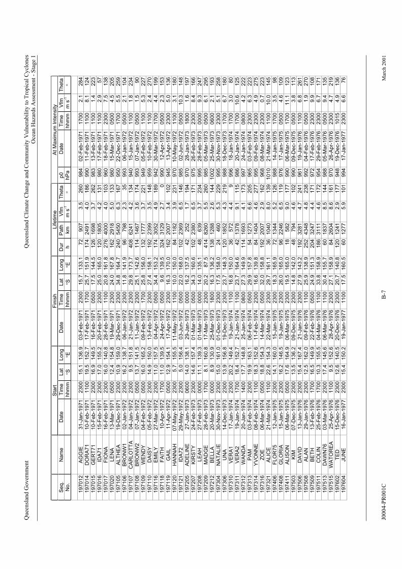
Quee
nsl
and G
over
nm
ent
Qu
een
slan
d C
lim
ate
Ch
ange
and
Co
mm
un
ity
Vuln
erab
ilit
y t
o T
rop
ical
Cy
clo
nes
Oce
an H
azar
ds
Ass
essm
ent
- S
tag
e 1
Sta
rtF
inis
hL
ife
tim
eA
t M
axim
um
In
ten
sity
Se
q.
Da
teT
ime
La
tL
on
gD
ate
Tim
eL
at
Lo
ng
Du
rP
ath
Vfm
Th
eta
p0
Da
teT
ime
Vfm
Th
eta
No
.h
hm
mS
Eh
hm
mS
Eh
km
ms
-1h
Pa
hh
mm
ms
-1
19
70
12
AG
GIE
31
-Ja
n-1
97
12
30
01
5.1
13
6.9
03
-Fe
b-1
97
12
30
01
5.7
13
3.1
72
90
73
.52
60
98
40
2-F
eb
-19
71
17
00
2.1
28
4
197014
DO
RA
71
10-F
eb
-1971
1100
19.5
152.7
17-F
eb
-1971
1700
25.7
151.9
174
2491
4.0
186
990
11-F
eb
-1971
1100
8.1
124
197015
GE
RT
71
10-F
eb
-1971
2300
16.9
149.5
16-F
eb
-1971
0500
17.5
144.5
126
1698
3.7
262
983
13-F
eb
-1971
1100
1.4
223
197016
IDA
71
15-F
eb
-1971
2300
17.0
155.2
20-F
eb
-1971
2300
25.0
165.0
120
1805
4.2
131
980
17-F
eb
-1971
1100
2.9
57
197017
FIO
NA
16-F
eb
-1971
2300
16.0
140.8
28-F
eb
-1971
1100
20.8
161.8
276
4000
4.0
103
960
18-F
eb
-1971
2300
7.5
138
197020
LE
NA
13-M
ar-
1971
0500
12.4
154.8
19-M
ar-
1971
2300
24.0
167.8
162
2918
5.0
133
980
15-M
ar-
1971
0500
4.5
205
19
71
05
AL
TH
EA
19
-De
c-1
97
12
30
01
0.9
15
9.0
29
-De
c-1
97
12
30
03
4.8
16
4.7
24
05
45
06
.31
67
95
02
2-D
ec-1
97
11
70
05
.52
59
19
71
06
BR
ON
W1
02
-Ja
n-1
97
22
30
01
6.2
13
8.7
06
-Ja
n-1
97
22
30
01
1.8
14
1.9
96
79
82
.33
59
93
06
-Ja
n-1
97
20
50
02
.11
04
19
71
07
CA
RL
OT
TA
04
-Ja
n-1
97
22
30
09
.51
51
.82
1-J
an
-19
72
23
00
29
.81
73
.74
08
62
41
4.2
13
49
40
15
-Ja
n-1
97
21
10
01
.82
34
19
71
08
BR
ON
W2
07
-Ja
n-1
97
20
50
01
3.7
14
1.5
11
-Ja
n-1
97
22
30
02
5.1
14
2.6
11
41
46
73
.61
74
99
30
7-J
an
-19
72
05
00
1.5
90
197109
WE
ND
Y04-F
eb
-1972
0500
16.0
165.2
09-F
eb
-1972
1700
25.8
156.0
132
1777
3.7
221
949
05-F
eb
-1972
1100
5.3
227
197110
DA
ISY
05-F
eb
-1972
2300
14.9
150.0
13-F
eb
-1972
2300
27.4
158.1
192
2399
3.5
148
959
10-F
eb
-1972
1100
2.4
270
197116
EM
ILY
27-M
ar-
1972
2300
11.0
157.5
04-A
pr-
1972
0500
34.4
153.2
174
3052
4.9
189
942
30-M
ar-
1972
1700
4.4
199
19
71
18
FA
ITH
10
-Ap
r-1
97
21
70
01
1.0
13
9.5
24
-Ap
r-1
97
20
50
09
.61
39
.53
24
31
29
2.7
09
90
12
-Ap
r-1
97
20
50
02
.31
53
19
71
19
GA
IL1
1-A
pr-
19
72
05
00
12
.91
54
.11
7-A
pr-
19
72
23
00
16
.31
70
.01
62
20
07
3.4
10
29
45
13
-Ap
r-1
97
22
30
05
.01
36
19
71
20
HA
NN
AH
07
-Ma
y-1
97
22
30
05
.71
55
.51
1-M
ay-1
97
21
10
01
0.0
15
0.0
84
11
82
3.9
23
19
70
10
-Ma
y-1
97
21
10
03
.11
80
19
71
21
IDA
72
29
-Ma
y-1
97
22
30
05
.01
56
.40
3-J
un
-19
72
05
00
22
.01
68
.01
02
23
69
6.5
14
69
85
02
-Ju
n-1
97
20
50
01
0.3
14
8
19
72
05
AD
EL
INE
27
-Ja
n-1
97
30
60
01
4.0
13
8.1
00
00
19
42
9-J
an
-19
73
16
.21
37
.54
22
52
1.7
97
02
8-J
an
-19
73
18
00
1.6
19
7
19
72
07
KIR
ST
Y2
4-F
eb
-19
73
23
00
14
.61
57
.40
50
001-M
ar-
1973
34.3
160.6
102
2380
6.5
171
975
26-F
eb
-1973
2300
8.4
166
19
72
08
LE
AH
27
-Fe
b-1
97
30
00
01
1.1
13
9.3
01
-Ma
r-1
97
30
00
01
4.0
13
5.1
48
00
00
639
3.7
234
995
28-F
eb
-1973
9.3
247
MA
DG
E1
70
08
.11
60
.81
7-M
ar-
19
73
23
00
20
.28
7.5
82
60
5.5
26
09
85
05
-Ma
r-1
97
36
.12
95
BE
LL
A2
0-M
ar-
19
73
00
00
8.9
13
0.9
25
-Ma
r-1
97
31
80
01
6.3
13
6.2
13
81
28
82
.61
44
10
02
25
-Ma
r-1
97
32
.1
19
73
04
NA
TA
LIE
30
-No
v-1
97
32
30
01
5.0
16
1.0
01
-De
c-1
97
32
30
01
7.5
15
8.0
24
46
05
.32
29
99
53
0-N
ov-1
97
32
30
05
.12
58
19
73
06
UN
A1
4-D
ec-1
97
32
30
01
3.9
15
6.8
19
-De
c-1
97
32
30
02
3.7
14
8.3
12
01
85
24
.32
19
98
81
8-D
ec-1
97
31
70
06
.71
80
19
73
10
VE
RA
11
7-J
an
-19
74
23
00
20
.21
49
.41
9-J
an
-19
74
11
00
16
.81
50
.03
65
72
4.4
99
96
18
-Ja
n-1
97
41
70
03
.08
0
19
73
11
VE
RA
21
9-J
an
-19
74
17
00
18
.41
52
.72
1-J
an
-19
74
42
11
00
23
.71
64
.61
37
89
.11
15
98
62
0-J
an
-19
74
17
00
10
.61
25
19
73
12
WA
ND
A2
0-J
an
-19
74
14
00
17
.71
48
.82
5-J
an
-19
74
08
00
27
.31
49
.91
14
16
93
4.1
17
39
97
24
-Ja
n-1
97
40
80
04
.22
22
197313
PA
M03-F
eb
-1974
2300
19.9
163.1
06-F
eb
-1974
0500
29.9
157.8
54
1273
6.6
205
965
03-F
eb
-1974
2300
6.3
223
197314
YV
ON
NE
08-F
eb
-1974
1100
18.3
152.6
11-F
eb
-1974
2300
16.6
139.8
84
1404
4.6
277
995
09-F
eb
-1974
2300
4.9
275
197316
ZO
E06-M
ar-
1974
0500
18.8
154.3
14-M
ar-
1974
0500
32.0
158.8
192
2007
2.9
162
968
08-M
ar-
1974
2300
0.7
223
197321
ALIC
E21-M
ar-
1974
1100
22.6
154.3
22-M
ar-
1974
2300
29.7
161.1
36
1040
8.0
139
1010
21-M
ar-
1974
1100
10.0
145
19
74
06
FL
OR
75
12
-Ja
n-1
97
52
30
01
4.1
16
0.0
15
-Ja
n-1
97
52
30
01
8.3
16
5.9
72
13
44
5.2
12
69
88
14
-Ja
n-1
97
51
70
03
.59
8
19
74
08
GL
OR
IA1
5-J
an
-19
75
23
00
16
.21
46
.51
9-J
an
-19
75
23
00
26
.01
65
.09
62
24
66
.51
19
97
61
7-J
an
-19
75
05
00
4.6
10
9
197411
ALIS
ON
06-M
ar-
1975
0500
17.6
164.9
06-M
ar-
1975
2300
19.5
165.0
18
582
9.0
177
990
06-M
ar-
1975
1700
11.1
123
19
75
03
KIM
07
-De
c-1
97
52
30
01
3.5
13
6.2
09
-De
c-1
97
52
30
01
4.8
14
2.0
48
79
44
.61
02
99
00
9-D
ec-1
97
50
50
03
.81
13
19
75
06
DA
VID
13
-Ja
n-1
97
62
30
01
5.4
16
7.4
21
-Ja
n-1
97
62
30
02
7.9
14
3.2
19
23
28
14
.72
41
96
11
9-J
an
-19
76
11
00
6.8
26
1
19
75
08
AL
AN
29
-Ja
n-1
97
62
30
01
2.5
16
2.0
09
-Fe
b-1
97
61
10
02
5.9
13
8.9
25
24
34
84
.82
38
99
20
4-F
eb
-19
76
05
00
1.9
27
0
197509
BE
TH
13-F
eb
-1976
1700
16.5
149.9
22-F
eb
-1976
0500
24.9
151.3
204
3247
4.4
171
972
17-F
eb
-1976
2300
9.9
108
197511
CO
LIN
25-F
eb
-1976
1700
10.3
155.5
04-M
ar-
1976
1100
33.8
158.9
186
3111
4.6
172
954
29-F
eb
-1976
2300
6.7
171
197513
DA
WN
76
03-M
ar-
1976
2300
17.4
145.6
06-M
ar-
1976
1100
30.4
155.7
60
1837
8.5
144
988
05-M
ar-
1976
0500
9.4
135
19
75
15
WA
TO
RE
A2
5-A
pr-
19
76
11
00
9.5
15
2.6
28
-Ap
r-1
97
62
30
02
7.1
15
8.9
84
26
04
8.6
16
19
70
26
-Ap
r-1
97
62
30
04
.72
19
19
76
02
TE
D1
5-D
ec-1
97
62
30
01
2.6
14
0.5
20
-De
c-1
97
62
30
02
0.7
14
0.8
12
01
24
12
.91
77
94
81
9-D
ec-1
97
61
01
54
.91
36
19
76
04
JU
NE
16
-Ja
n-1
97
72
30
01
5.4
15
0.2
19
-Ja
n-1
97
71
10
01
7.5
16
0.5
60
12
77
5.9
10
19
94
17
-Ja
n-1
97
72
30
06
.67
6
Na
me
197209
28-F
eb
-1973
414
0500
19
72
12
06
00
19
3
J0004-P
R001C
B-7
Mar
ch 2
00
1
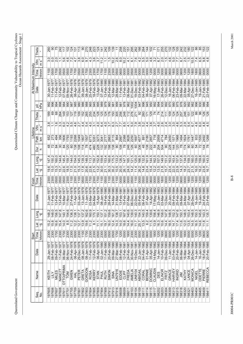
Quee
nsl
and G
over
nm
ent
Qu
een
slan
d C
lim
ate
Ch
ange
and
Co
mm
un
ity
Vuln
erab
ilit
y t
o T
rop
ical
Cy
clo
nes
Oce
an H
azar
ds
Ass
essm
ent
- S
tag
e 1
Sta
rtF
inis
hL
ife
tim
eA
t M
axim
um
In
ten
sity
Se
q.
Da
teT
ime
La
tL
on
gD
ate
Tim
eL
at
Lo
ng
Du
rP
ath
Vfm
Th
eta
p0
Da
teT
ime
Vfm
Th
eta
No
.h
hm
mS
Eh
hm
mS
Eh
km
ms
-1h
Pa
hh
mm
ms
-1
19
76
05
KE
ITH
29
-Ja
n-1
97
72
30
01
5.2
14
8.2
31
-Ja
n-1
97
72
30
01
9.6
14
7.4
48
65
23
.81
89
99
23
0-J
an
-19
77
11
00
3.0
26
0
197606
LIL
Y08-F
eb
-1977
2300
15.8
148.0
11-F
eb
-1977
2300
15.0
150.2
72
273
1.1
69
996
11-F
eb
-1977
0500
0.0
90
197607
MIL
ES
09-F
eb
-1977
1700
16.6
156.5
13-F
eb
-1977
0500
15.3
160.0
84
494
1.6
68
994
11-F
eb
-1977
1700
2.0
75
197608
NA
NC
77
11-F
eb
-1977
2300
15.4
147.8
13-F
eb
-1977
0500
15.7
144.6
30
356
3.3
264
998
12-F
eb
-1977
0500
1.1
242
OT
TO
(PR
IMA
06
-Ma
r-1
97
71
70
01
4.0
14
0.1
10
-Ma
r-1
97
70
50
02
2.6
14
5.4
84
18
06
6.0
14
99
84
07
-Ma
r-1
97
70
50
05
.61
17
19
77
01
TO
M0
6-N
ov-1
97
72
30
08
.51
54
.61
1-N
ov-1
97
72
30
01
8.5
15
9.7
12
01
79
34
.21
53
99
00
9-N
ov-1
97
70
50
04
.61
02
197705
GW
EN
24-F
eb
-1978
2300
11.2
136.3
27-F
eb
-1978
1100
17.0
144.0
60
1193
5.5
127
987
26-F
eb
-1978
1700
7.2
124
197709
HA
L06-A
pr-
1978
0500
12.2
138.1
11-A
pr-
1978
2300
21.0
154.0
138
2268
4.6
119
985
06-A
pr-
1978
1700
4.7
131
19
78
01
PE
TE
R2
9-D
ec-1
97
82
30
01
2.7
13
7.7
03
-Ja
n-1
97
91
10
01
5.3
14
5.3
10
81
04
92
.71
09
98
03
1-D
ec-1
97
80
50
03
.81
13
19
78
02
GR
ET
A0
8-J
an
-19
79
11
00
13
.91
37
.21
3-J
an
-19
79
05
00
17
.81
39
.31
14
18
07
4.4
15
29
86
09
-Ja
n-1
97
92
30
06
.09
0
19
78
03
GO
RD
ON
08
-Ja
n-1
97
91
70
01
9.6
16
2.6
11
-Ja
n-1
97
92
30
02
0.6
14
8.5
78
15
07
5.4
26
59
88
08
-Ja
n-1
97
91
70
09
.72
70
197804
RO
SA
11-F
eb
-1979
23
00
2300
11.2
160.9
03-M
ar-
1979
1700
22.6
113.7
474
6773
4.0
255
965
25-F
eb
-1979
4.3
248
197805
KE
RR
Y12-F
eb
-1979
2300
8.1
170.1
04-M
ar-
1979
2300
21.5
945
2300
15
0.7
48
05
35
13
.12
34
18
-Fe
b-1
97
93
.62
23
19
78
09
ST
AN
06
-Ap
r-1
97
90
50
01
1.1
15
0.1
15
-Ap
r-1
97
91
70
01
3.2
15
2.8
22
83
27
34
.01
28
99
51
3-A
pr-
19
79
17
00
3.7
12
4
19
79
04
PA
UL
02
-Ja
n-1
98
02
30
01
5.1
13
7.1
08
-Ja
n-1
98
01
10
03
0.0
15
9.6
13
23
04
16
.41
25
98
90
7-J
an
-19
80
17
00
11
.21
41
197909
RU
TH
11-F
eb
-1980
0500
19.7
151.2
19-F
eb
-1980
0500
21.1
153.4
192
2777
4.0
124
979
13-F
eb
-1980
1100
1.1
242
197912
SIM
ON
20-F
eb
-1980
0500
16.0
159.6
28-F
eb
-1980
1100
30.3
160.6
198
960
14-M
ar-
1980
54
71
83
.77
49
92
16
-Ma
y-1
98
20
00
03
.27
1
19
82
02
DE
S1
4-J
an
-19
83
12
00
16
.31
46
.92
3-J
an
-19
83
00
00
13
.51
57
.02
04
29
59
4.0
74
99
41
7-J
an
-19
83
12
00
6.7
17
1
198203
ELIN
OR
10-F
eb
-1983
1800
10.6
158.0
03-M
ar-
1983
1800
21.8
149.9
504
4714
2.6
214
935
26-F
eb
-1983
0000
2.0
255
19
83
04
FR
ITZ
09
-De
c-1
98
30
60
01
4.4
14
7.8
13
-De
c-1
98
30
00
01
5.7
15
1.2
90
78
42
.41
11
99
21
2-D
ec-1
98
30
60
01
.52
70
19
83
09
GR
AC
E1
1-J
an
-19
84
00
00
18
.51
48
.52
0-J
an
-19
84
12
00
23
.41
63
.02
28
24
50
3.0
10
99
70
16
-Ja
n-1
98
40
60
04
.61
32
198313
HA
RV
EY
03-F
eb
-1984
1800
14.7
152.3
09-F
eb
-1984
1800
22.0
163.4
144
1571
3.0
124
980
06-F
eb
-1984
1800
5.0
128
198315
ING
RID
20-F
eb
-1984
1200
17.4
147.6
25-F
eb
-1984
1200
23.9
157.6
120
1968
4.6
124
975
23-F
eb
-1984
0000
7.7
105
19
83
18
JIM
06
-Ma
r-1
98
40
00
01
1.6
15
0.7
09
-Ma
r-1
98
40
60
01
4.3
13
7.8
78
14
94
5.3
25
79
76
09
-Ma
r-1
98
40
60
06
.72
42
198320
KA
TH
Y16-M
ar-
1984
1800
12.0
148.5
24-M
ar-
1984
0000
18.2
134.0
174
1824
2.9
246
920
22-M
ar-
1984
1200
2.5
232
198321
LA
NC
E04-A
pr-
1984
0000
13.5
153.4
07-A
pr-
1984
1800
23.7
159.3
90
1761
5.4
151
992
05-A
pr-
1984
1200
1.5
180
19
84
03
MO
NIC
A2
6-D
ec-1
98
40
00
01
4.5
14
8.5
28
-De
c-1
98
41
20
02
1.5
16
0.0
60
14
47
6.7
12
29
82
27
-De
c-1
98
41
80
01
0.5
12
2
19
84
04
NIG
EL
14
-Ja
n-1
98
51
20
01
6.5
15
0.3
16
-Ja
n-1
98
51
80
01
6.0
15
9.0
54
93
34
.88
69
96
16
-Ja
n-1
98
51
80
07
.48
6
19
84
05
OD
ET
TE
16
-Ja
n-1
98
51
20
01
4.6
14
5.6
19
-Ja
n-1
98
51
20
01
6.2
15
9.8
72
15
55
6.0
96
93
01
9-J
an
-19
85
06
00
6.5
85
198409
PIE
RR
E18-F
eb
-1985
0600
11.8
143.3
24-F
eb
-1985
0600
23.8
160.0
144
2492
4.8
126
986
21-F
eb
-1985
0000
9.8
153
198411
RE
BE
CC
A20-F
eb
-1985
0600
11.1
135.7
23-F
eb
-1985
1200
16.7
143.5
78
1268
4.5
126
994
22-F
eb
-1985
0000
4.8
122
Na
me
19
76
11
2663
3.7
176
25-F
eb
-1980
2300
1.5
109
19
79
13
SIN
A0
9-M
ar-
19
80
05
00
12
.41
61
.22
30
03
5.2
17
5.5
13
83
11
56
.31
50
98
11
2-M
ar-
19
80
23
00
10
.21
39
197916
UN
7916
27-M
ar-
1980
1700
14.3
138.7
31-M
ar-
1980
1100
10.5
133.2
90
864
2.7
305
999
28-M
ar-
1980
0500
2.6
11
198008
ED
DIE
08-F
eb
-1981
1200
14.0
153.1
13-F
eb
-1981
0000
20.0
126.5
108
2997
7.7
256
981
11-F
eb
-1981
0600
8.0
258
198009
CLIF
F12-F
eb
-1981
0000
18.6
167.6
15-F
eb
-1981
0600
26.1
147.3
78
2388
8.5
248
978
13-F
eb
-1981
0000
10.2
220
198011
FR
ED
A24-F
eb
-1981
1800
14.4
140.6
07-M
ar-
1981
0000
24.0
165.1
246
3626
4.1
112
962
06-M
ar-
1981
4.1
00
00
15
1
19
81
03
AM
EL
IA3
0-N
ov-1
98
12
30
01
6.0
13
9.0
06
-De
c-1
98
10
50
01
4.2
12
1.5
01
-De
c-1
98
16
.11
26
22
50
5.0
27
61
00
20
50
02
95
19
81
04
UN
81
04
19
-De
c-1
98
12
30
01
1.7
14
0.3
22
-De
c-1
98
11
10
01
1.4
12
5.0
60
16
97
7.9
27
11
00
41
9-D
ec-1
98
12
30
07
.62
62
19
81
09
AB
IGA
IL9
22
2-J
an
-19
82
00
00
25
.71
54
.30
5-F
eb
-19
82
00
00
26
.21
66
.53
36
45
77
3.8
94
70
3-F
eb
-19
82
00
00
4.2
16
6
198111
CO
RA
L04-F
eb
-1982
0500
13.5
140.5
06-F
eb
-1982
0500
14.8
132.8
48
891
5.2
260
996
04-F
eb
-1982
2300
5.5
264
19
81
14
BE
RN
IE0
1-A
pr-
19
82
06
00
6.2
15
9.4
07
-Ap
r-1
98
20
00
02
3.4
16
1.9
13
82
18
04
.41
71
94
50
6-A
pr-
19
82
00
00
5.0
14
4
19
81
15
DO
MIN
IC0
5-A
pr-
19
82
00
00
11
.51
39
.61
4-A
pr-
19
82
06
00
15
.41
44
.52
22
28
57
3.6
12
99
50
07
-Ap
r-1
98
21
20
04
.61
02
19
81
17
CL
AU
DIA
14
-Ma
y-1
98
21
80
01
3.9
15
6.4
17
-Ma
y-1
98
20
00
01
2.2
16
2.5
J0004-P
R001C
B-8
Mar
ch 2
00
1

Quee
nsl
and G
over
nm
ent
Qu
een
slan
d C
lim
ate
Ch
ange
and
Co
mm
un
ity
Vuln
erab
ilit
y t
o T
rop
ical
Cy
clo
nes
Oce
an H
azar
ds
Ass
essm
ent
- S
tag
e 1
Sta
rtF
inis
hL
ife
tim
eA
t M
axim
um
In
ten
sity
Se
q.
Da
teT
ime
La
tL
on
gD
ate
Tim
eL
at
Lo
ng
Du
rP
ath
Vfm
Th
eta
p0
Da
teT
ime
Vfm
Th
eta
No
.h
hm
mS
Eh
hm
mS
Eh
km
ms
-1h
Pa
hh
mm
ms
-1
19
84
14
SA
ND
Y2
0-M
ar-
19
85
18
00
13
.41
38
.21
35
.11
20
024-M
ar-
1985
1800
14.5
96
766
2.2
249
953
22-M
ar-
1985
2.6
191
198415
TA
NY
A27-M
ar-
1985
0600
13.2
151.5
01-A
pr-
1985
1800
15.2
142.8
132
1082
2.3
256
982
30-M
ar-
1985
0600
2.6
281
19
85
05
VE
RN
ON
21
-Ja
n-1
98
60
00
01
6.5
13
9.5
24
-Ja
n-1
98
61
80
02
4.0
16
0.0
90
23
65
7.3
11
19
90
24
-Ja
n-1
98
60
00
01
3.2
11
7
19
85
06
WIN
IFR
ED
27
-Ja
n-1
98
60
60
01
2.9
14
4.8
05
-Fe
b-1
98
61
80
02
0.9
14
4.2
22
82
00
92
.41
84
95
70
1-F
eb
-19
86
07
00
4.5
26
0
198511
ALF
RE
D02-M
ar-
1986
1800
14.8
150.2
08-M
ar-
1986
0000
18.5
164.0
126
1628
3.6
105
992
07-M
ar-
1986
1800
10.6
112
198513
MA
NU
21-A
pr-
1986
0000
8.0
156.0
27-A
pr-
1986
0000
16.0
144.6
144
1584
3.1
234
970
24-A
pr-
1986
1200
3.4
242
19
85
15
NA
MU
16
-Ma
y-1
98
61
80
07
.01
63
.92
2-M
ay-1
98
60
00
01
8.4
16
5.4
12
62
06
84
.61
72
96
02
0-M
ay-1
98
61
20
06
.61
57
19
86
02
IRM
A1
9-J
an
-19
87
06
00
12
.61
39
.02
1-J
an
-19
87
00
00
15
.41
34
.14
26
56
4.3
23
99
94
19
-Ja
n-1
98
71
20
03
.12
60
198604
JA
SO
N05-F
eb
-1987
1800
12.0
142.8
14-F
eb
-1987
0000
21.1
139.4
198
2028
2.8
199
965
12-F
eb
-1987
1200
2.9
135
19
86
07
BL
AN
CH
21
-Ma
y-1
98
70
60
01
0.1
16
6.8
27
-Ma
y-1
98
70
00
01
9.9
15
7.0
13
81
93
13
.92
24
99
02
2-M
ay-1
98
71
80
02
.52
16
19
87
01
AG
I0
8-J
an
-19
88
00
00
15
.01
57
.01
4-J
an
-19
88
06
00
19
.51
62
.01
50
21
64
4.0
13
39
80
12
-Ja
n-1
98
81
80
06
.61
48
198704
CH
AR
LIE
21-F
eb
-1988
0000
12.8
159.1
01-M
ar-
1988
1800
20.9
147.5
234
2085
2.5
233
972
29-F
eb
-1988
1200
1.1
154
19
88
02
DE
LIL
AH
28
-De
c-1
98
81
80
01
6.7
14
8.4
01
-Ja
n-1
98
91
20
01
8.4
16
0.0
90
16
71
5.2
98
98
80
1-J
an
-19
89
06
00
10
.01
01
198806
HA
RR
Y13-F
eb
-1989
0600
19.7
160.3
17-F
eb
-1989
0600
20.9
160.4
96
927
2.7
175
925
14-F
eb
-1989
0000
2.0
284
19
88
09
AIV
U0
1-A
pr-
19
89
12
00
12
.11
52
.00
5-A
pr-
19
89
12
00
22
.01
42
.29
61
62
44
.72
23
93
50
3-A
pr-
19
89
06
00
4.7
19
2
19
88
11
ME
EN
A0
5-M
ay-1
98
90
00
01
3.4
16
0.0
10
-Ma
y-1
98
90
60
01
1.5
13
7.4
12
62
64
05
.82
74
99
00
6-M
ay-1
98
90
60
05
.73
15
19
88
12
ER
NIE
09
-Ma
y-1
98
91
80
01
2.0
15
5.6
12
-Ma
y-1
98
91
20
01
2.3
14
8.8
66
12
17
5.1
26
79
98
11
-Ma
y-1
98
90
00
08
.62
70
19
89
02
FE
LIC
ITY
13
-De
c-1
98
90
00
01
1.6
13
4.0
19
-De
c-1
98
91
20
02
0.2
16
0.2
15
63
36
66
.01
08
97
51
5-D
ec-1
98
90
60
05
.61
17
19
89
06
NA
NC
90
28
-Ja
n-1
99
00
60
01
8.3
15
6.0
04
-Fe
b-1
99
01
20
03
4.5
15
5.0
17
44
05
46
.51
83
97
50
1-F
eb
-19
90
06
00
8.4
26
6
198907
GR
EG
01-M
ar-
1990
1800
11.9
137.9
03-M
ar-
1990
0000
12.1
139.8
30
225
2.1
96
992
03-M
ar-
1990
0000
1.8
124
198910
HIL
DA
04-M
ar-
1990
0000
18.8
153.2
07-M
ar-
1990
1800
26.0
165.0
90
1831
5.7
123
970
06-M
ar-
1990
0000
1.8
54
198912
IVO
R16-M
ar-
1990
0000
15.8
160.8
26-M
ar-
1990
1200
21.9
146.8
252
4075
4.5
245
965
19-M
ar-
1990
0000
5.0
264
19
90
02
JO
Y1
9-D
ec-1
99
00
60
01
2.3
15
2.8
26
-De
c-1
99
00
60
01
9.2
14
7.5
16
81
32
72
.22
16
94
02
3-D
ec-1
99
00
00
01
.01
80
19
90
05
KE
LV
IN2
5-F
eb
-19
91
06
00
15
.51
49
.40
5-M
ar-
19
91
12
00
14
.01
49
.71
98
16
66
2.3
10
98
02
6-F
eb
-19
91
18
00
2.5
30
7
19
90
10
LIS
A0
8-M
ay-1
99
10
60
01
0.3
15
4.3
11
-Ma
y-1
99
10
00
01
6.8
15
9.1
66
10
26
4.3
14
49
75
10
-Ma
y-1
99
10
60
04
.91
14
19
91
02
MA
RK
07
-Ja
n-1
99
21
20
01
3.3
13
6.1
10
-Ja
n-1
99
21
80
01
3.3
14
3.5
78
87
03
.19
09
80
09
-Ja
n-1
99
21
80
04
.35
3
19
91
03
BE
TS
Y1
0-J
an
-19
92
12
00
19
.51
60
.01
4-J
an
-19
92
06
00
27
.61
60
.09
01
17
83
.61
80
95
01
0-J
an
-19
92
12
00
5.0
25
8
199104
DA
MA
N15-F
eb
-1992
0600
13.1
168.5
19-F
eb
-1992
1200
31.6
157.0
102
2634
7.2
209
965
17-F
eb
-1992
1800
8.8
215
19
91
06
ES
AU
26
-Fe
b-1
99
20
60
01
5.5
16
7.3
04
-Ma
r-1
99
20
00
01
9.8
16
5.3
16
21
98
03
.42
03
92
52
8-F
eb
-19
92
12
00
1.8
32
7
199108
FR
AN
09-M
ar-
1992
0600
18.6
168.3
17-M
ar-
1992
1200
25.5
159.0
198
2872
4.0
231
950
11-M
ar-
1992
1800
2.5
258
19
92
02
NIN
A0
00
01
3.0
14
0.0
02
-Ja
n-1
99
31
80
01
1.5
17
1.0
25
84
00
04
.38
79
60
31
-De
c-1
99
21
80
07
.75
7
199204
OLIV
ER
05-F
eb
-1993
0000
15.0
150.1
12-F
eb
-1993
1800
22.0
154.6
186
1549
2.3
148
945
07-F
eb
-1993
1200
2.1
223
199205
PO
LL
Y25-F
eb
-1993
0000
16.0
158.0
02-M
ar-
1993
0000
24.3
165.5
120
1355
3.1
139
955
01-M
ar-
1993
0000
5.7
154
199206
RO
GE
R12-M
ar-
1993
0000
10.0
157.0
21-M
ar-
1993
0000
21.3
160.9
216
2737
3.5
161
975
15-M
ar-
1993
0000
1.5
180
19
93
01
RE
WA
28
-De
c-1
99
30
60
09
.51
65
.52
1-J
an
-19
94
12
00
29
.01
58
.05
82
89
58
4.3
20
09
20
02
-Ja
n-1
99
41
20
04
.81
62
19
93
02
SA
DIE
29
-Ja
n-1
99
40
60
01
2.3
13
7.8
31
-Ja
n-1
99
41
20
02
0.1
14
2.5
54
11
23
5.8
14
99
85
30
-Ja
n-1
99
41
80
05
.31
63
19
93
03
TH
EO
DO
RE
23
-Fe
b-1
99
40
60
01
0.5
15
4.6
27
-Fe
b-1
99
40
30
02
2.7
16
8.1
93
21
48
6.4
13
39
10
25
-Fe
b-1
99
40
60
04
.31
35
19
94
01
VIO
LE
T0
3-M
ar-
19
95
06
00
16
.01
52
.50
8-M
ar-
19
95
00
00
29
.21
55
.11
14
26
48
6.5
16
99
60
05
-Ma
r-1
99
51
20
01
0.0
15
7
199402
WA
RR
EN
04-M
ar-
1995
0000
13.3
140.1
06-M
ar-
1995
0100
17.2
137.8
49
781
4.4
209
960
05-M
ar-
1995
1700
6.7
242
19
94
03
AG
NE
S1
7-A
pr-
19
95
00
00
11
.81
47
.32
1-A
pr-
19
95
00
00
12
.11
47
.69
64
56
1.3
13
59
45
18
-Ap
r-1
99
51
80
00
.09
0
19
95
01
BA
RR
Y0
3-J
an
-19
96
00
00
15
.01
36
.80
9-J
an
-19
96
00
00
23
.11
47
.51
44
16
41
3.2
12
89
50
05
-Ja
n-1
99
60
70
04
.31
36
19
95
02
CE
LE
ST
E2
6-J
an
-19
96
12
00
18
.21
46
.32
8-J
an
-19
96
01
00
19
.21
51
.33
76
20
4.7
10
19
60
27
-Ja
n-1
99
60
80
05
.89
0
199503
DE
NN
IS15-F
eb
-1996
0000
11.8
140.3
18-F
eb
-1996
0600
15.6
151.0
78
1311
4.7
110
990
16-F
eb
-1996
1200
4.8
108
Na
me
23
-De
c-1
99
2
J0004-P
R001C
B-9
Mar
ch 2
00
1

Quee
nsl
and G
over
nm
ent
Qu
een
slan
d C
lim
ate
Ch
ange
and
Co
mm
un
ity
Vuln
erab
ilit
y t
o T
rop
ical
Cy
clo
nes
Oce
an H
azar
ds
Ass
essm
ent
- S
tag
e 1
Sta
rtF
inis
hL
ife
tim
eA
t M
axim
um
In
ten
sity
Se
q.
Da
teT
ime
La
tL
on
gD
ate
Tim
eL
at
Lo
ng
Du
rP
ath
Vfm
Th
eta
p0
Da
teT
ime
Vfm
Th
eta
No
.h
hm
mS
Eh
hm
mS
Eh
km
ms
-1h
Pa
hh
mm
ms
-1
199504
ET
HE
L07-M
ar-
1996
1800
15.8
139.5
13-M
ar-
1996
0600
17.2
136.3
132
2285
4.8
245
980
09-M
ar-
1996
1800
6.1
80
19
96
01
FE
RG
US
22
-De
c-1
99
62
10
01
1.3
16
0.8
30
-De
c-1
99
61
20
03
8.0
17
7.0
18
34
73
57
.21
51
97
52
5-D
ec-1
99
60
00
08
.18
2
19
96
02
DR
EN
A0
2-J
an
-19
97
00
00
10
.01
72
.00
9-J
an
-19
97
06
00
29
.11
68
.31
74
38
43
6.1
19
09
35
06
-Ja
n-1
99
70
00
02
.01
80
199603
GIL
LIA
N09-F
eb
-1997
0600
12.5
150.5
12-F
eb
-1997
1800
19.3
146.8
84
896
3.0
207
995
11-F
eb
-1997
0600
3.3
201
199604
HA
RO
LD
16-F
eb
-1997
0600
13.6
157.8
22-F
eb
-1997
1200
33.4
166.8
150
2830
5.2
157
975
18-F
eb
-1997
1800
4.0
120
199605
ITA
23-F
eb
-1997
1200
15.1
148.3
24-F
eb
-1997
1800
20.0
146.6
30
640
5.9
198
994
24-F
eb
-1997
1200
5.3
219
199606
JU
ST
IN06-M
ar-
1997
1800
17.0
153.5
23-M
ar-
1997
2300
19.2
147.3
413
3679
2.5
249
955
17-M
ar-
1997
1200
3.9
337
19
97
01
NU
TE
18
-No
v-1
99
70
00
01
1.1
16
5.1
20
-No
v-1
99
71
20
01
8.5
15
8.3
60
11
51
5.3
22
19
75
19
-No
v-1
99
70
60
04
.32
33
19
97
02
SID
24
-De
c-1
99
70
60
01
3.5
13
0.8
28
-De
c-1
99
72
10
01
6.2
13
7.1
11
11
79
74
.51
13
98
52
8-D
ec-1
99
70
00
05
.81
48
19
97
03
KA
TR
INA
02
-Ja
n-1
99
80
00
01
5.0
15
2.0
29
-Ja
n-1
99
80
00
01
7.2
14
9.6
64
86
71
92
.92
26
94
01
5-J
an
-19
98
12
00
3.0
21
0
19
97
04
LE
S1
9-J
an
-19
98
00
00
13
.01
38
.02
9-J
an
-19
98
12
00
14
.51
27
.62
52
28
47
3.1
26
19
82
24
-Ja
n-1
99
81
20
04
.82
51
199705
MA
Y24-F
eb
-1998
1800
13.1
139.1
07-M
ar-
1998
0000
14.8
136.3
246
2271
2.6
238
990
26-F
eb
-1998
0600
5.9
150
199706
NA
TH
AN
20-M
ar-
1998
1800
11.1
143.3
31-M
ar-
1998
0000
13.8
145.0
246
3498
4.0
148
990
21-M
ar-
1998
0600
1.5
90
19
98
01
OL
IND
A2
0-J
an
-19
99
09
00
17
.21
58
.31
80
01
59
21
-Ja
n-1
99
91
9.8
15
9.3
33
31
02
.69
87
21
-Ja
n-1
99
91
80
03
.21
62
19
98
02
PE
TE
21
-Ja
n-1
99
90
00
01
5.0
14
9.0
18
00
23
-Ja
n-1
99
92
2.7
15
9.8
66
15
10
6.4
12
69
85
23
-Ja
n-1
99
90
60
07
.41
28
199803
RO
NA
09-F
eb
-1999
1100
15.1
146.8
12-F
eb
-1999
1100
15.8
145.0
72
1200
876
3.4
248
970
11-F
eb
-1999
5.0
275
FR
AN
K1200
21.5
150.1
18-F
eb
-1999
1200
20.2
159.8
1039
6.0
81
994
18-F
eb
-1999
3.4
90
ST
EV
E2
5-F
eb
-20
00
00
00
17
.21
53
.02
9-F
eb
-20
00
12
00
16
.51
39
.11
08
17
04
4.4
27
39
80
27
-Fe
b-2
00
07
.9
19
99
02
VA
UG
HA
N2
8-M
ar-
20
00
23
00
20
.01
68
.00
7-A
pr-
20
00
00
00
14
.61
46
.32
17
28
39
3.6
28
49
75
05
-Ap
r-2
00
01
80
04
.02
62
19
99
03
TE
SS
I3
1-M
ar-
20
00
00
00
14
.81
56
.20
3-A
pr-
20
00
12
00
17
.51
43
.58
41
50
75
.02
57
98
00
2-A
pr-
20
00
20
00
0.0
90
Na
me
199804
16-F
eb
-1999
48
0600
19
99
01
09
00
27
0
J0004-P
R001C
B-1
0M
arch
20
01

Queensland Government Queensland Climate Change and Community Vulnerability to Tropical CyclonesOcean Hazards Assessment - Stage 1
Appendix C Tropical Cyclone Wind and Pressure Model
The following provides an overview of the parametric tropical cyclone wind and pressure model adopted for this study, which is similar to Harper and Holland (1999). Further elaboration is provided here of specific formulations which have been developed over a number of years as a result of extensive wind, wave and current hindcasting, e.g. Harper et al.
(1989, 1993) and Harper (1999).
C.1 Definitions and Background
A tropical cyclone (hurricane or typhoon) is defined as a non-frontal cyclonically rotating (clockwise in the Southern Hemisphere) low pressure system (below 1000 hPa) of tropical origin, in which 10 min mean wind speeds at +10 m MSL (V km h34 kn, or 17.5 m s plex nature of tropical cyclones and their interactionwith surrounding synoptic scale mechanisms, most empirical wind and pressure models(Lovell 1990) represent the surface wind field by considering the storm as a steadyaxisymmetric vortex which is stationary in a fluid at rest.
where r = radial distance from storm centre
p = ambient surrounding pressure field
This exponential pressure profile was first proposed by Schloemer (1954). Holland (1980) noted deficiencies in the ability of Equation C.1 to represent many observed pressure profiles and that the Schloemer base-profiles resembled a family of rectangular hyperbolae, viz:
m) exceed gale force (63 -1,-1). In view of the com
The vortex solution is based on the Eulerian equations of motion in a rotating frame of reference (Smith 1968). The analysis begins with a consideration of force balance at the geostrophic, or gradient, wind level above the influence of the planetary boundary layer. The gradient wind speed can be expressed as a function of storm pressure, size, air density and latitude. The gradient wind speed is then reduced to the surface reference level of +10 mMSL (mean sea level) by consideration of gross boundary layer effects, wind inflow (also due to frictional effects) and asymmetric effects due to storm forward motion or surrounding synoptic pressure gradients.
C.2 Radial Pressure Field
A primary assumption of almost all empirical tropical cyclone models is that the radial pressure field at gradient wind speed level can be expressed as:
p(r) = p0 + (pn - p0) exp (-R/r) (C.1)
p(r) = pressure at r
p0 = pressure at the storm centre (central pressure)
n
and R = radius to maximum winds
rB ln [p/( pn - p0)] = A (C.2)
where A and B are storm-dependent scaling parameters.
This modification leads to the following radial pressure field, which forms the basis of the'Holland' model:
J0004-PR001C C-1 March 2001
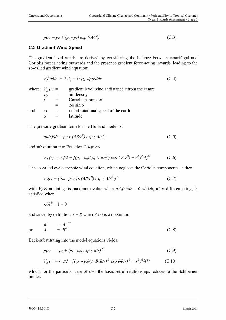
Queensland Government Queensland Climate Change and Community Vulnerability to Tropical CyclonesOcean Hazards Assessment - Stage 1
= 2 sin
V ) = [(p /r exp (-A/r
p(r) = p0 + (pn - p0) exp (-A/rB) (C.3)
C.3 Gradient Wind Speed
The gradient level winds are derived by considering the balance between centrifugal andCoriolis forces acting outwards and the presence gradient force acting inwards, leading to the so-called gradient wind equation:
Vg2(r)/r + f Vg = 1/ a dp(r)/dr (C.4)
where Vg (r) = gradient level wind at distance r from the centre
a = air densityf = Coriolis parameter
and = radial rotational speed of the earth
= latitude
The pressure gradient term for the Holland model is:
dp(r)/dr = p / r (AB/rB) exp (-A/r
B) (C.5)
and substituting into Equation C.4 gives
Vg (r) = -r f/2 + [(pn - p0)/ a (AB/rB) exp (-A/r
B) + r
2 f
2/4]
½ (C.6)
The so-called cyclostrophic wind equation, which neglects the Coriolis components, is then
c(r n - p0)/ a (ABB)
B)]
½ (C.7)
with Vc(r) attaining its maximum value when dVc(r)/dr = 0 which, after differentiating, is satisfied when
-A/rB + 1 = 0
and since, by definition, r = R when Vc(r) is a maximum
R = A1/B
or A = RB (C.8)
Back-substituting into the model equations yields:
p(r) = p0 + (pn - p0) exp (-R/r) B (C.9)
Vg (r) = -r f/2 +[( pn - p0)/ a B(R/r) B
exp (-R/r) B
+ r2 f
2/4]
½ (C.10)
which, for the particular case of B=1 the basic set of relationships reduces to the Schloemermodel.
J0004-PR001C C-2 March 2001
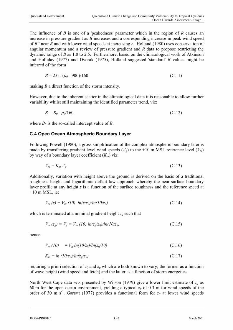
Queensland Government Queensland Climate Change and Community Vulnerability to Tropical CyclonesOcean Hazards Assessment - Stage 1
The influence of B is one of a 'peakedness' parameter which in the region of R causes anincrease in pressure gradient as B increases and a corresponding increase in peak wind speedof B R and with lower wind speeds at increasing r. Holland (1980) uses conservation of angular momentum and a review of pressure gradient and R data to propose restricting the dynamic range of B as 1.0 to 2.5. Furthermore, based on the climatological work of Atkinson and Holliday (1977) and Dvorak (1975), Holland suggested 'standard' B values might beinferred of the form
However, due to the inherent scatter in the climatological data it is reasonable to allow furthervariability whilst still maintaining the identified parameter trend, viz:
which is terminated at a nominal gradient height z at
½ near
B = 2.0 - (p0 - 900)/160 (C.11)
making B a direct function of the storm intensity.
B = B0 - p0/160 (C.12)
where B0 is the so-called intercept value of B.
C.4 Open Ocean Atmospheric Boundary Layer
Following Powell (1980), a gross simplification of the complex atmospheric boundary later is made by transferring gradient level wind speeds (Vg) to the +10 m MSL reference level (Vm)by way of a boundary layer coefficient (Km) viz:
Vm = Km Vg (C.13)
Additionally, variation with height above the ground is derived on the basis of a traditional roughness height and logarithmic deficit law approach whereby the near-surface boundary layer profile at any height z is a function of the surface roughness and the reference speed at +10 m MSL, ie:
Vm (z) = Vm (10) ln(z/z0)/ln(10/z0) (C.14)
g such th
Vm (zg) = Vg = Vm (10) ln(zg/z0)/ln(10/z0) (C.15)
hence
Vm (10) = Vg ln(10/z0)/ln(zg/10) (C.16)
Km = ln (10/z0)/ln(zg/z0) (C.17)
requiring a priori selection of z0 and zg which are both known to vary; the former as a function of wave height (wind speed and fetch) and the latter as a function of storm energetics.
North West Cape data sets presented by Wilson (1979) give a lower limit estimate of zg as 60 m for the open ocean environment, yielding a typical z0 of 0.3 m for wind speeds of the order of 30 m s-1. Garratt (1977) provides a functional form for z0 at lower wind speeds
J0004-PR001C C-3 March 2001
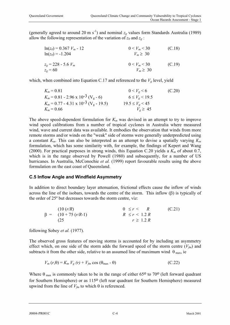
Queensland Government Queensland Climate Change and Community Vulnerability to Tropical CyclonesOcean Hazards Assessment - Stage 1
(generally agreed to around 20 m s-1) and nominal zg values form Standards Australia (1989) allow the following representation of the variation of z0 and zg :
ln(z V 0 < Vm < 30 (C.18)
z V 0 < Vm < 30 (C.19)
0) = 0.367 m - 12
ln(z0) = -1.204 Vm 30
g = 228 - 5.6 m
zg = 60 Vm 30
which, when combined into Equation C.17 and referenced to the Vg level, yield
Km = 0.81 0 < Vg < 6 (C.20)
Km = 0.81 - 2.96 x 10⁻³ (Vg - 6) 6 Vg < 19.5
Km = 0.77 - 4.31 x 10⁻³ (Vg - 19.5) 19.5 Vg < 45
Km = 0.66 Vg 45
The above speed-dependent formulation for Km was devised in an attempt to try to improve wind speed calibrations from a number of tropical cyclones in Australia where measuredwind, wave and current data was available. It embodies the observation that winds from moreremote storms and/or winds on the "weak" side of storms were generally underpredicted using a constant Km. This can also be interpreted as an attempt to devise a spatially varying Km
formulation, which has some similarity with, for example, the findings of Kepert and Wang(2000). For practical purposes in strong winds, this Equation C.20 yields a Km of about 0.7, which is in the range observed by Powell (1980) and subsequently, for a number of US hurricanes. In Australia, McConochie et al. (1999) report favourable results using the above formulation on the east coast of Queensland.
C.5 Inflow Angle and Windfield Asymmetry
In addition to direct boundary layer attenuation, frictional effects cause the inflow of winds
across the line of the isobars, towards the centre of the storm. This inflow ( ) is typically ofthe order of 25º but decreases towards the storm centre, viz:
(10 (r/R) 0 r < R (C.21)
= (10 + 75 (r/R-1) R r < 1.2 R
(25 r 1.2 R
following Sobey et al. (1977).
The observed gross features of moving storms is accounted for by including an asymmetryeffect which, on one side of the storm adds the forward speed of the storm centre (Vfm) and
subtracts it from the other side, relative to an assumed line of maximum wind max, ie
Vm (r, ) = Km Vg (r) + Vfm cos ( max - ) (C.22)
Where max is commonly taken to be in the range of either 65o to 70o (left forward quadrant
for Southern Hemisphere) or as 115o (left rear quadrant for Southern Hemisphere) measured
upwind from the line of Vfm to which is referenced.
J0004-PR001C C-4 March 2001
Queensland Government Queensland Climate Change and Community Vulnerability to Tropical CyclonesOcean Hazards Assessment - Stage 1
Figure C.1 presents the geometry of the wind field model in detail, including consideration of
north point references for fm and Vb (the bearing of Vm).
C.6 References
Atkinson G.D. and Holliday C.R. (1977) Tropical cyclone minimum sea level pressure/maximum sustained wind relationship for the Western North Pacific. Monthly
Weather Review, 105, 421-427.
Dvorak V.F. (1975) Tropical cyclone intensity analysis and forecasting from satellite imagery.Monthly Weather Review, 103, 420-430.
Garratt J.R. (1977) Review of drag coefficients over oceans and continents.Monthly Weather Review, 105, 915-929.
Harper B.A., Lovell, K.F., Chandler B.D. and Todd D.J. (1989) The derivation of environmental design criteria for Goodwyn 'A' Platform, Proc. 9th Aust Conf. Coastal and Ocean Engin., Institution of Engineers Australia, Adelaide, Dec.
Harper B.A., Mason L.B. and Bode L. (1993) Tropical cyclone Orson - a severe test for modelling, Proc. 11th Australian Conf. on Coastal and Ocean Engin., Institution of Engineers
Australia, Townsville, Aug, 59-64.
Harper B.A. (1999) Numerical modelling of extreme tropical cyclone winds. APSWE SpecialEdition, Journal of Wind Engineering and Industrial Aerodynamics, 83, 35 - 47.
Harper B.A. and Holland G.J. (1999) An updated parametric model of the tropical cyclone. Proc. 23rd Conf. Hurricanes and Tropical Meteorology, American Meteorological Society,Dallas, Texas, 10-15 Jan.
Holland G.J (1980) An analytic model of the wind and pressure profiles in hurricanes. Monthly Weather Review, 108, 1212-1218.
Kepert J.D. and Wang Y. (2000) The dynamics of boundary layer jets within the tropical cyclone core. Part II: Nonlinear enhancement. To appear Jnl Atmospheric Science.
Lovell K.F. (1990) Review of empirical tropical cyclone wind and pressure models. MEngSt Thesis, Dept Civil Engineering, University of Western Australia.
McConochie J.D., Mason L.B. and Hardy T.A. (1999) A Coral Sea wind model intended forwave modelling. Proc. 14th Australasian Conf. Coastal and Ocean Enginering, IEAust, Perth,April, 413-418.
NOAA (1979) Meteorological criteria for standard project hurricane and probable maximumhurricane windfields, Gulf and East Coasts of the United States", NOAA Tech Rep NWS23,US Dept of Commerce, Sept.
Powell, M.D. (1980) Evaluations of diagnostic marine boundary-layer models applied to hurricanes. Monthly Weather Review, 108, 757-766.
J0004-PR001C C-5 March 2001
Queensland Government Queensland Climate Change and Community Vulnerability to Tropical CyclonesOcean Hazards Assessment - Stage 1
Schloemer R.W. (1954) Analysis and synthesis of hurricane wind patterns over Lake Okeechobee, Florida. US Weather Bureau, March.
Smith R.K. (1968) The surface boundary layer of a hurricane. Tellus, 0, 473-484.
Sobey R.J., Harper B.A. and Stark K.P. (1977) Numerical simulation of tropical cyclone storm surge. Research Bulletin CS-14, Dept Civil and Systems Engineering, James Cook
University, March.
Standards Australia (1989) AS 1170.2 - 1989 SAA loading code part 2: wind loads. 96 pp.
Wilson K.J. (1979) Wind observations from an instrumented tower during tropical cyclone Karen, 1977. 12th Tech Conf on Hurricanes and Tropical Meteorology, American
Meteorological Society, New Orleans, April.
J0004-PR001C C-6 March 2001
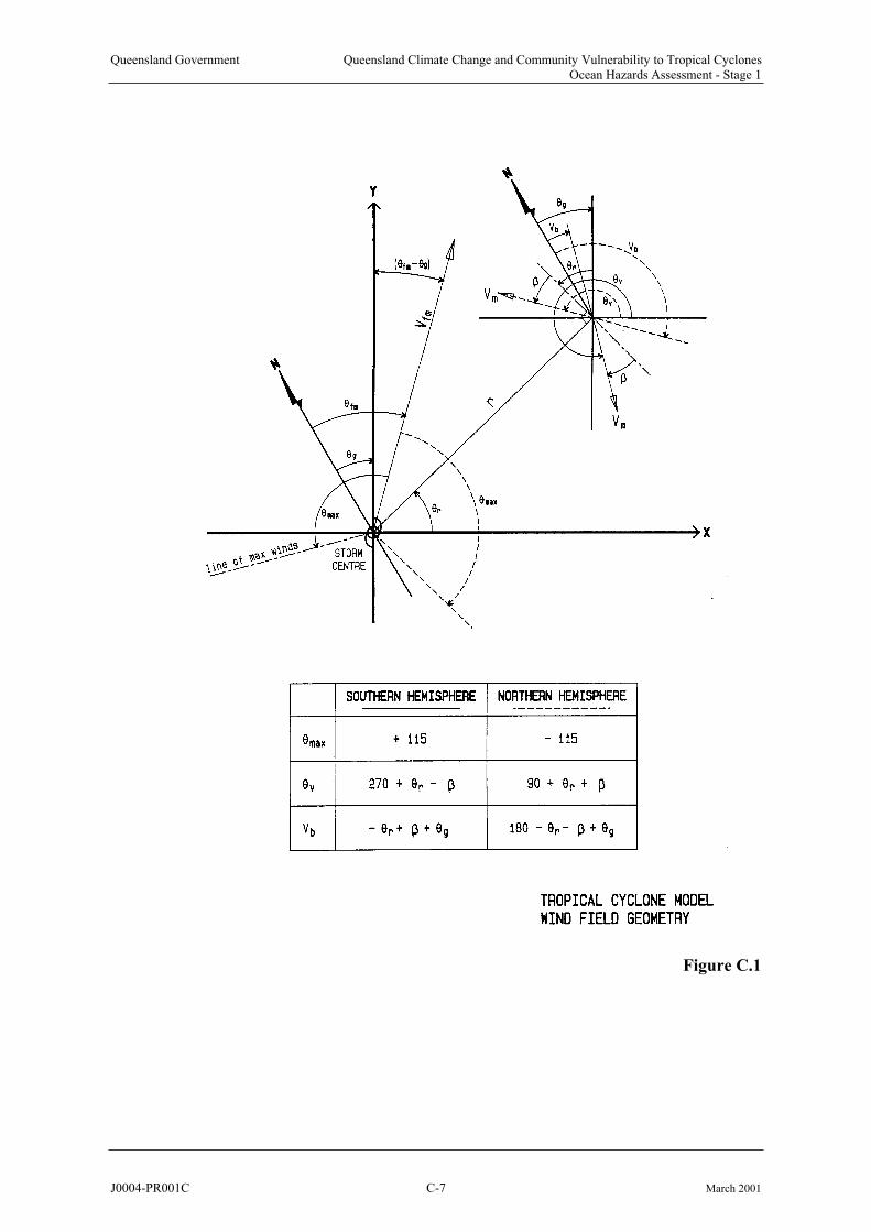
Queensland Government Queensland Climate Change and Community Vulnerability to Tropical CyclonesOcean Hazards Assessment - Stage 1
Figure C.1
J0004-PR001C C-7 March 2001

Queensland Government Queensland Climate Change and Community Vulnerability to Tropical CyclonesOcean Hazards Assessment - Stage 1
Appendix D Technical Description of the James Cook University Storm Surge Model (MMUSURGE)
D.1 Introduction
This appendix describes the basis of the 2D depth integrated hydrodynamic model(MMUSURGE) developed by the Marine Modelling Unit at the School of Engineering, JamesCook University. The model is based on the depth integrated equations of motion using the usual assumption that the fluid is incompressible and homogeneous. It is formulated in a spherical coordinate system and includes all the basic momentum terms such as Coriolis,advection, horizontal diffusion, surface and bottom stress and the inverse barometer effect. Wind stress is parameterised through a quadratic drag law using the drag coefficient of Wu (1982). Bottom friction is also parameterised using a quadratic friction law with the drag coefficient coming from the assumption of a logarithmic profile. One unique aspect of thismodel is its ability to include the effects of sub-grid scale reef and barriers on water flow.
The model has a built-in tropical cyclone wind field model and a built-in uniform wind field model. The tropical cyclone wind field is based on that of Holland, consistent with Appendix C, with modifications that make it suitable for the Coral Sea region. The model is capable ofproducing output that includes water levels and velocities. The output can be in the form oftime histories or full gridded output. The User Guide (Mason and McConochie 2001) provides specific detail of how to incorporate varying surface wind and pressure fields.
D.2 Equations of Motion
The equations of motion are the two-dimensional (2D) long wave equations, describing conservation of momentum and mass for a homogeneous fluid. In the present work, these equations are formulated in standard spherical polar coordinates, used in models over significant portions of the earth's surface.
By the use of the hydrostatic approximation, the equations become:
2
tancos
cos
( ),
cos
e s s bm h
U U U V U UV
t D a D a aD
U U D V DfV
D t D a D a
pgD A
aU
(D.1)
2
2
tancos
cos
( ),
s be sm h
V U V V V U
t D a D a aD
V U D V DfU
D t D a D a
pgD A
aV
(D.2)
1 cos0.
cos
U V
t a(D.3)
Here: is east longitude; is latitude; t is time; D = - h is total water depth; is the
surface elevation, relative to Mean Sea Level (MSL) datum; h is the bottom elevation; D is
J0004-PR001C D-1 March 2001

Queensland Government Queensland Climate Change and Community Vulnerability to Tropical CyclonesOcean Hazards Assessment - Stage 1
the minimum average or effective depth where sub-grid scale reef or barriers are included;
the components of transport (U and V) are, defined by (U, V) = D(u, v), where u = (u, v) is
depth averaged fluid velocity; f is the Coriolis parameter (equal to 2 sin , where = 7.292
10-5 s-1 is the earth’s angular velocity); a is the earth’s radius; e is the equilibrium tide
height; ps is atmospheric pressure; is the density of seawater; Am is the horizontal eddy
viscosity; and denotes the horizontal Laplacian operator.2
h
At the water surface, wind stress ( )s , when required, is modelled conventionally through the
quadratic drag law,
10 10 10 ,s aC W W (D.4)
where is the wind at a standard anemometer height of 10 m, 10
W a is the density of air and
C10 is the surface drag coefficient. The (dimensionless) drag coefficient is a function of the magnitude of the wind speed. The formula used in the present study is that of Wu (1982):
3
10 100.8 0.065 10 ,C W (D.5)
where the magnitude of W is given in m s10
-1. At the sea bed, the bottom shear stress ( b) is
expressed in terms of the total near bottom transport Q = (U 2 + V2)0.5 and total water depth
D, by the quadratic friction law:
, 2( ) ( ,
b
b b b
C QU V
D) (D.6)
where Cb is a drag coefficient. For fully developed turbulent flow, the near bottom currents are very closely approximated by a logarithmic profile. From this relationship, it can beshown that the drag coefficient can then be expressed as:
2
0( / )b
b
CIn z z
(D.7)
where = 0.4 is the well known von Karman constant, zb is the elevation of the lowest horizontal transports (Ub, Vb), and z0 is the bottom roughness length. The physical or
Nikuradse roughness is approximately equal to 30z0.
When no partial (sub-grid scale) barriers or reefs are defined, =1and =1, otherwise they are given by
312
1
1bw
bw
w (D.8)
and
0.56
12
1
1 1.56b
b ww
1 .w (D.9)
Here , the end effects, is defined as 2
11
1 1
1 11 11 ln 2ln
1 4
ww
w w w
1
1
w (D.10)
and the modified gap fractions are 2
1 31 , 1 , ,reef
bed
breeftt h
h bed
CDRw w w R w w w R R
R D C. (D.11) t
b
The reef gap fraction, w, and reef width fraction, b, are related to the proportion of the grid space taken up by reefs or barriers.
J0004-PR001C D-2 March 2001
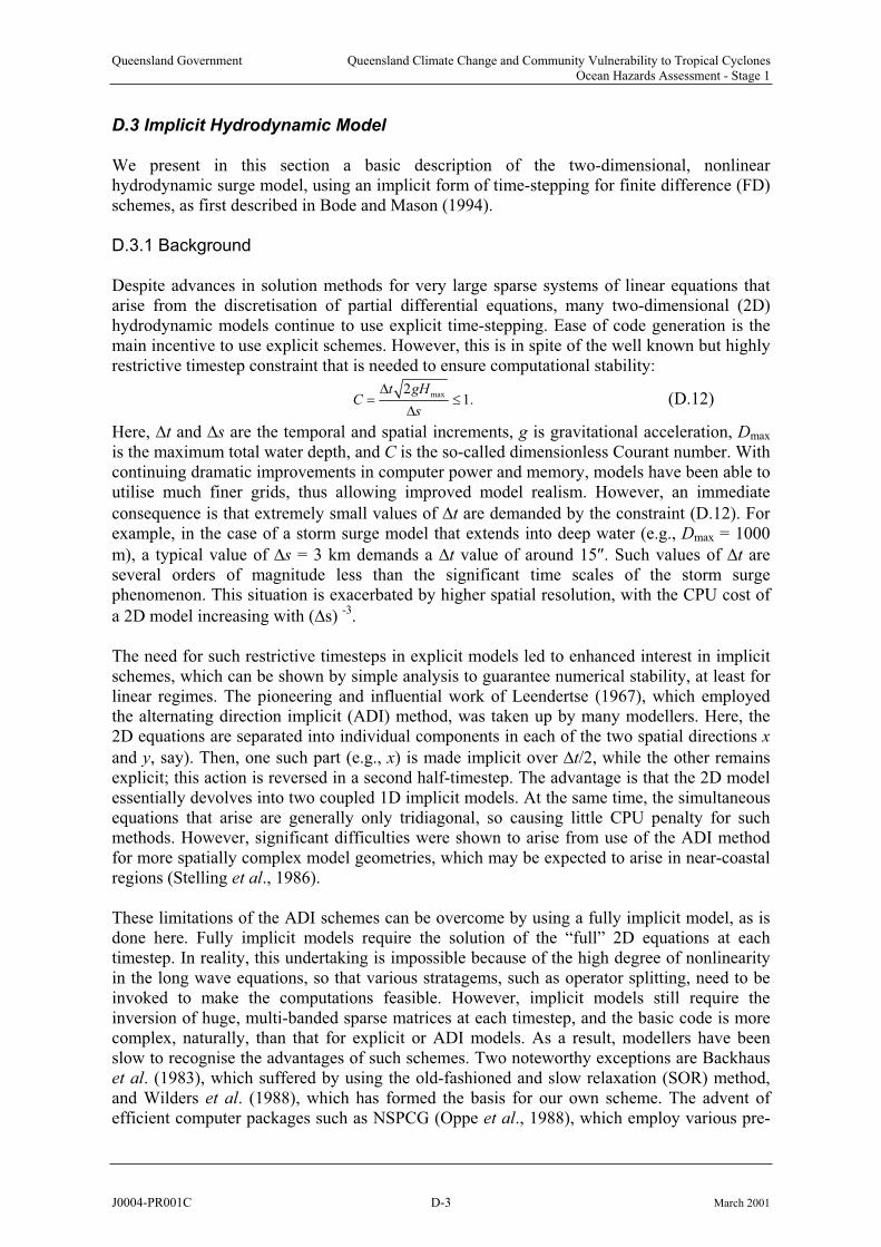
Queensland Government Queensland Climate Change and Community Vulnerability to Tropical CyclonesOcean Hazards Assessment - Stage 1
D.3 Implicit Hydrodynamic Model
We present in this section a basic description of the two-dimensional, nonlinear hydrodynamic surge model, using an implicit form of time-stepping for finite difference (FD) schemes, as first described in Bode and Mason (1994).
D.3.1 Background
Despite advances in solution methods for very large sparse systems of linear equations that arise from the discretisation of partial differential equations, many two-dimensional (2D) hydrodynamic models continue to use explicit time-stepping. Ease of code generation is the main incentive to use explicit schemes. However, this is in spite of the well known but highly restrictive timestep constraint that is needed to ensure computational stability:
max21.
t gHC
s(D.12)
Here, t and s are the temporal and spatial increments, g is gravitational acceleration, Dmax
is the maximum total water depth, and C is the so-called dimensionless Courant number. Withcontinuing dramatic improvements in computer power and memory, models have been able toutilise much finer grids, thus allowing improved model realism. However, an immediate
consequence is that extremely small values of t are demanded by the constraint (D.12). Forexample, in the case of a storm surge model that extends into deep water (e.g., Dmax = 1000
m), a typical value of s = 3 km demands a t value of around 15 . Such values of t are several orders of magnitude less than the significant time scales of the storm surge phenomenon. This situation is exacerbated by higher spatial resolution, with the CPU cost of
a 2D model increasing with ( s) -3.
The need for such restrictive timesteps in explicit models led to enhanced interest in implicitschemes, which can be shown by simple analysis to guarantee numerical stability, at least forlinear regimes. The pioneering and influential work of Leendertse (1967), which employedthe alternating direction implicit (ADI) method, was taken up by many modellers. Here, the 2D equations are separated into individual components in each of the two spatial directions x
and y, say). Then, one such part (e.g., x) is made implicit over t/2, while the other remainsexplicit; this action is reversed in a second half-timestep. The advantage is that the 2D modelessentially devolves into two coupled 1D implicit models. At the same time, the simultaneous equations that arise are generally only tridiagonal, so causing little CPU penalty for such methods. However, significant difficulties were shown to arise from use of the ADI methodfor more spatially complex model geometries, which may be expected to arise in near-coastalregions (Stelling et al., 1986).
These limitations of the ADI schemes can be overcome by using a fully implicit model, as is done here. Fully implicit models require the solution of the “full” 2D equations at eachtimestep. In reality, this undertaking is impossible because of the high degree of nonlinearity in the long wave equations, so that various stratagems, such as operator splitting, need to be invoked to make the computations feasible. However, implicit models still require the inversion of huge, multi-banded sparse matrices at each timestep, and the basic code is morecomplex, naturally, than that for explicit or ADI models. As a result, modellers have been slow to recognise the advantages of such schemes. Two noteworthy exceptions are Backhaus et al. (1983), which suffered by using the old-fashioned and slow relaxation (SOR) method,and Wilders et al. (1988), which has formed the basis for our own scheme. The advent of efficient computer packages such as NSPCG (Oppe et al., 1988), which employ various pre-
J0004-PR001C D-3 March 2001

Queensland Government Queensland Climate Change and Community Vulnerability to Tropical CyclonesOcean Hazards Assessment - Stage 1
conditioned conjugate gradient schemes for the solution of large banded systems of equations,has now made implicit models much more feasible than in the past.
D.3.2 Model description
We illustrate the numerical model scheme with the full equations of motion used in the stormsurge simulations, although for notational simplicity we employ the Cartesian form of these, rather than the spherical. The equations are:
2 ( ) 1,sx bx
U U UVfV gD
t x D y D x (D.13)
2 1,sy by
V UV VfU gD
t x D y D y (D.14)
0.U V
t x y(D.15)
Notation is as follows: t is time; U and V are the components of horizontal transport or depth-
integrated velocity; the water column extends from the sea surface at z= (x,y) to the sea floor
at z=-h(x,y), giving a total water depth of D = h + ; f is the Coriolis parameter, with f -
4.8 10-5 s-1 at the latitude of Townsville; s = ( sx, sy) is surface stress due to the wind; b =
( bx, by) is the seabed stress. We follow accepted 2D modelling practice and set 1 2
2 2
2, ,b
U VU V
D (D.16)
where is the density of seawater (assumed constant), and is a weakly depth-dependent
dimensionless drag coefficient -- typical values lie around 2.5 10-3 (Sobey et al., 1977). The basic geometric layout is depicted in the schematic below (Figure D.1).
Figure D.1 Schematic layout of model geometry in cartesian coordinates (x,y,z). The
water column of total depth D extends from the free surface, z = (x,y,t), to the sea floor, z = -h(x,y). The vertical datum is depicted here as Mean Sea Level (MSL), z = 0. Also shown are
the surface and bottom stresses, s and b, and the transport, U = (U,V).
Our method is based on that described in Wilders et al. (1988), but with some significant modifications. Changes from the original 2D scheme of Wilders et al. (1988) include the use
J0004-PR001C D-4 March 2001

Queensland Government Queensland Climate Change and Community Vulnerability to Tropical CyclonesOcean Hazards Assessment - Stage 1
of transport rather than velocity components as prognostic variables, and an implicit methodfor treating the Coriolis terms. The numerical FD scheme consists of a combination of explicit and implicit steps, which combine to produce trapezoidal or Crank-Nicolson time
differencing. In the horizontal, the prognostic variables U, V and are specified on a spatiallystaggered finite difference grid (the standard Arakawa `C' arrangement -- Mesinger andArakawa (1976) – as shown in Figure D.2.
Figure D.2 Space-time distribution of U, V and variables on the C-grid.
Use of a C-grid greatly simplifies coastal boundary conditions in coastal ocean modelling, although the Coriolis terms then require spatial averaging, which can cause complicationswith implicit models. A method that has been devised to overcome such problems on a
staggered grid is described in brief below. We assume here a square spatial grid ( x= y =
s), although this restriction can be easily relaxed, and define variables on the discrete space-time grid in standard fashion,
, , , , , ,n
p q p q nx y t p s q s n t (D.17)
and similarly for U and V at their corresponding positions. We use the flow chart of Figure D.3 to describe the implementation of the scheme, where we define an intermediate andtemporary half-timestep, by t* = tn+1/2. The steps then proceed sequentially, as indicated on this diagram.
Figure D.3 Sequence of operations over one timestep for the split implicit FD scheme.
J0004-PR001C D-5 March 2001
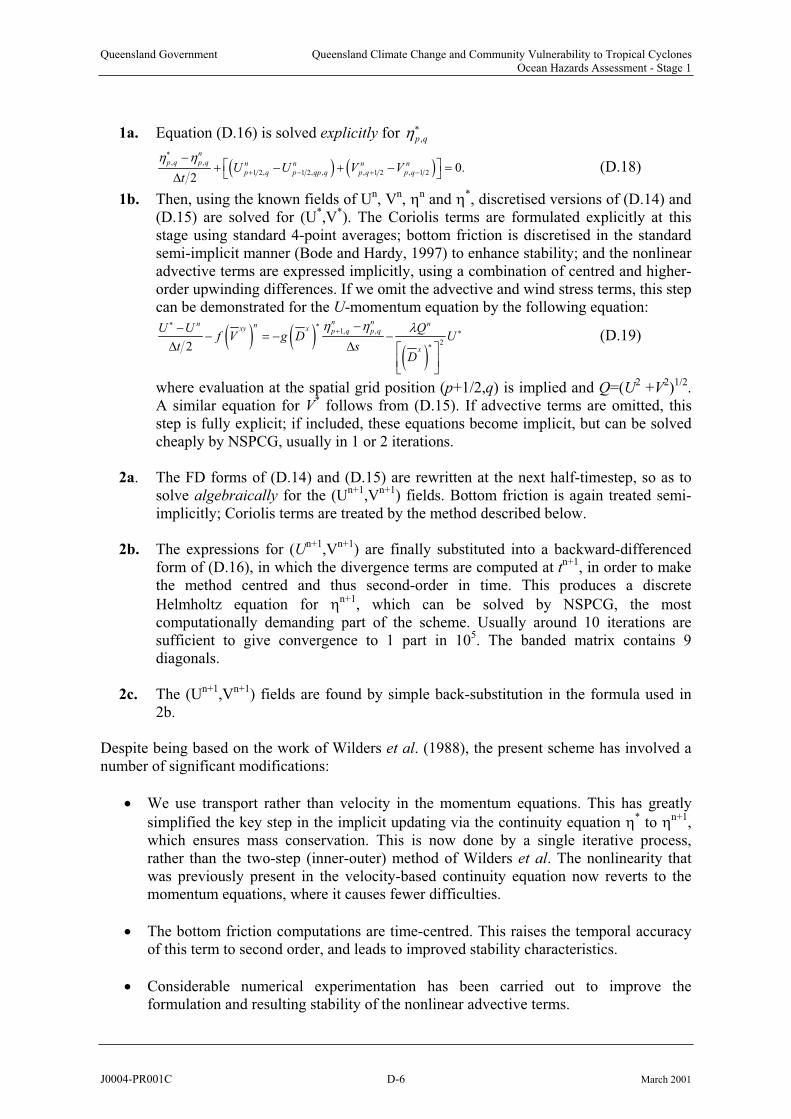
Queensland Government Queensland Climate Change and Community Vulnerability to Tropical CyclonesOcean Hazards Assessment - Stage 1
1a. Equation (D.16) is solved explicitly for ,p q
, ,
1 2, 1 2, , , 1 2 , 1 2 0.2
n
p q p q n n n n
p q p qp q p q p qU U V Vt
n1b. Then, using the known fields of U ,
(D.15) are solved for (U s are formulated explicitly at this stage using standard 4-point averages; bottom friction is discretised in the standard semi-implicit manner (Bode and Hardy, 1997) to enhance stability; and the nonlinearadvective terms are expressed implicitly, using a combination of centred and higher-order upwinding differences. If we omit the advective and wind stress terms, this stepcan be demonstrated for the U-momentum equation by the following equation:
(D.18)
n, V n and *, discretised versions of (D.14) and *,V*). The Coriolis term
1, ,
22
n nn nnxy x p q p q
x
U U Qf V g D U
t sD
(D.19)
where evaluation at the spatial grid position (p+1/2,q) is implied and Q=(U2 +V2)1/2.
A similar equation for V* follows from (D.15). If advective terms are omitted, thisstep is fully explicit; if included, these equations become implicit, but can be solved cheaply by NSPCG, usually in 1 or 2 iterations.
2a. The FD forms of (D.14) and (D.15) are rewritten at the next half-timestep, so as to solve algebraically for the (Un+1,Vn+1) fields. Bottom friction is again treated semi-implicitly; Coriolis terms are treated by the method described below.
2b. The expressions for (Un+1,Vn+1) are finally substituted into a backward-differencedform of (D.16), in which the divergence terms are computed at tn+1, in order to makethe method centred and thus second-order in time. This produces a discrete
Helmholtz equation for n+1, which can be solved by NSPCG, the mostcomputationally demanding part of the scheme. Usually around 10 iterations are sufficient to give convergence to 1 part in 105. The banded matrix contains 9 diagonals.
2c. The (Un+1,Vn+1) fields are found by simple back-substitution in the formula used in 2b.
Despite being based on the work of Wilders et al. (1988), the present scheme has involved a number of significant modifications:
We use transport rather than velocity in the momentum equations. This has greatly
simplified the key step in the implicit updating via the continuity equation * to n+1,which ensures mass conservation. This is now done by a single iterative process,rather than the two-step (inner-outer) method of Wilders et al. The nonlinearity that was previously present in the velocity-based continuity equation now reverts to themomentum equations, where it causes fewer difficulties.
The bottom friction computations are time-centred. This raises the temporal accuracyof this term to second order, and leads to improved stability characteristics.
Considerable numerical experimentation has been carried out to improve the formulation and resulting stability of the nonlinear advective terms.
J0004-PR001C D-6 March 2001
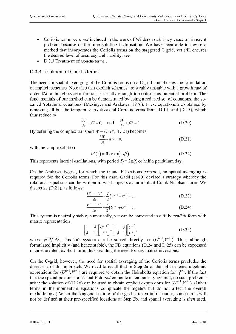
Queensland Government Queensland Climate Change and Community Vulnerability to Tropical CyclonesOcean Hazards Assessment - Stage 1
Coriolis terms were not included in the work of Wilders et al. They cause an inherentproblem because of the time splitting factorisation. We have been able to devise a method that incorporates the Coriolis terms on the staggered C grid, yet still ensures the desired level of accuracy and stability, see
D.3.3 Treatment of
D.3.3 Treatment of Coriolis terms
Coriolis terms .
The need for spatial averaging of the Coriolis terms on a C-grid complicates the formulationof implicit schemes. Note also that explicit schemes are weakly unstable with a growth rate of
order f t, although system friction is usually enough to control this potential problem. The fundamentals of our method can be demonstrated by using a reduced set of equations, the so-called ‘rotational equations’ (Mesinger and Arakawa, 1976). These equations are obtained by removing all but the temporal derivative and Coriolis terms from (D.14) and (D.15), which thus reduce to
0,U
fVt
and 0.V
fUt
(D.20)
By defining the complex transport W = U+iV, (D.21) becomes
0,W
ifWt
(D.21)
with the simple solution
0 exp .W t W ift (D.22)
This represents inertial oscillations, with period Tf = 2 /f, or half a pendulum day.
On the Arakawa B-grid, for which the U and V locations coincide, no spatial averaging isrequired for the Coriolis terms. For this case, Gadd (1980) devised a strategy whereby the rotational equations can be written in what appears as an implicit Crank-Nicolson form. Wediscretise (D.21), as follows:
11 0,
2
n nn nU U f
V Vt
(D.23)
11 0.
2
n nn nV V f
U Ut
(D.24)
This system is neutrally stable, numerically, yet can be converted to a fully explicit form with matrix representation
n
U1
1
1 1,
1 1
n n
n
U
V V(D.25)
where =2f t. This 2 2 system can be solved directly for (Un+1,Vn+1). Thus, although formulated implicitly (and hence stable), the FD equations (D.24 and D.25) can be expressed in an equivalent explicit form, thus avoiding the need for any matrix inversions.
On the C-grid, however, the need for spatial averaging of the Coriolis terms precludes the direct use of this approach. We need to recall that in Step 2a of the split scheme, algebraic
expressions for (Un+1,Vn+1) are required to obtain the Helmholtz equation for n+1. If the factthat the spatial positions of U and V do not coincide is temporarily ignored, no such problemsarise: the solution of (D.26) can be used to obtain explicit expressions for (Un+1,Vn+1). (Otherterms in the momentum equations complicate the algebra but do not affect the overall methodology.) When the staggered nature of the grid is taken into account, some terms will not be defined at their pre-specified locations at Step 2b, and spatial averaging is then used,
J0004-PR001C D-7 March 2001
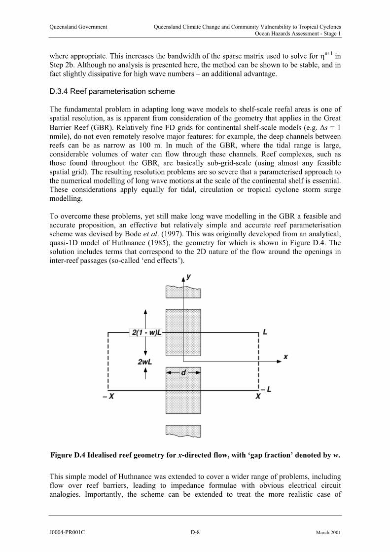
Queensland Government Queensland Climate Change and Community Vulnerability to Tropical CyclonesOcean Hazards Assessment - Stage 1
where appropriate. This increases the bandwidth of the sparse matrix used to solve for n+1 inStep 2b. Although no analysis is presented here, the method can be shown to be stable, and in fact slightly dissipative for high wave numbers – an additional advantage.
D.3.4 Reef parameterisation scheme
The fundamental problem in adapting long wave models to shelf-scale reefal areas is one of spatial resolution, as is apparent from consideration of the geometry that applies in the Great
Barrier Reef (GBR). Relatively fine FD grids for continental shelf-scale models (e.g. s = 1nmile), do not even remotely resolve major features: for example, the deep channels between reefs can be as narrow as 100 m. In much of the GBR, where the tidal range is large, considerable volumes of water can flow through these channels. Reef complexes, such asthose found throughout the GBR, are basically sub-grid-scale (using almost any feasible spatial grid). The resulting resolution problems are so severe that a parameterised approach to the numerical modelling of long wave motions at the scale of the continental shelf is essential. These considerations apply equally for tidal, circulation or tropical cyclone storm surge modelling.
To overcome these problems, yet still make long wave modelling in the GBR a feasible and accurate proposition, an effective but relatively simple and accurate reef parameterisationscheme was devised by Bode et al. (1997). This was originally developed from an analytical, quasi-1D model of Huthnance (1985), the geometry for which is shown in Figure D.4. Thesolution includes terms that correspond to the 2D nature of the flow around the openings in inter-reef passages (so-called ‘end effects’).
Figure D.4 Idealised reef geometry for x-directed flow, with ‘gap fraction’ denoted by w.
This simple model of Huthnance was extended to cover a wider range of problems, including flow over reef barriers, leading to impedance formulae with obvious electrical circuit analogies. Importantly, the scheme can be extended to treat the more realistic case of
J0004-PR001C D-8 March 2001
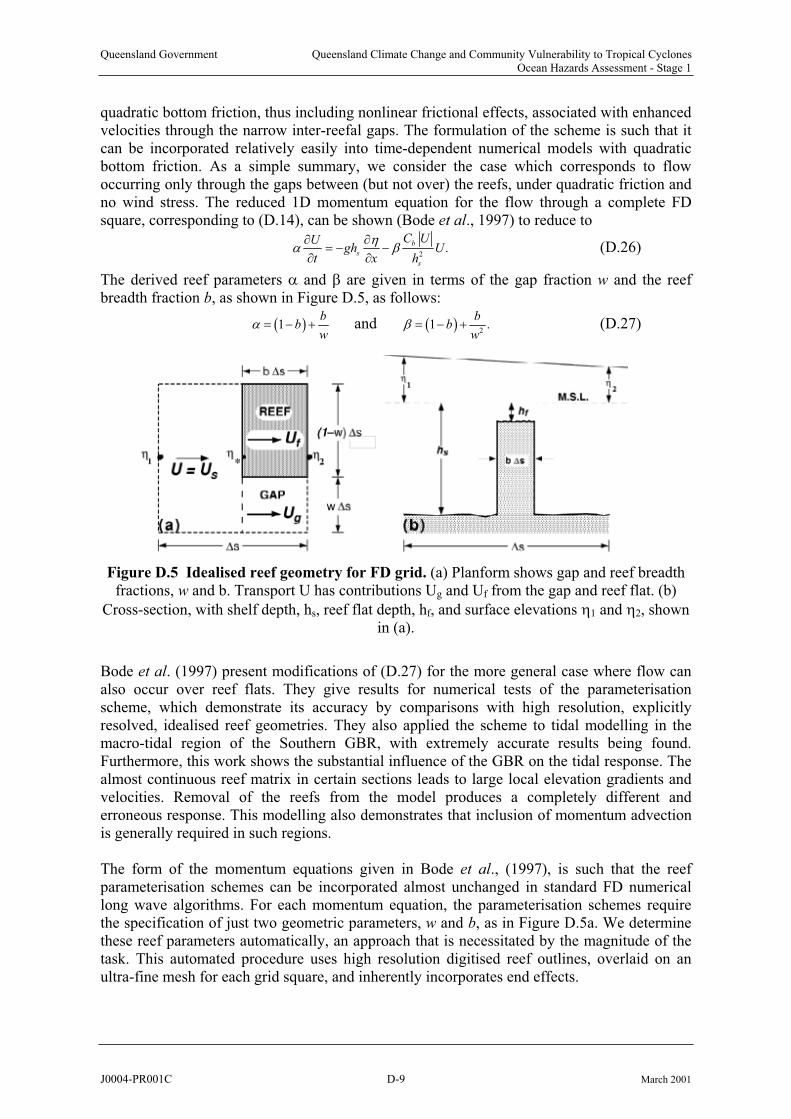
Queensland Government Queensland Climate Change and Community Vulnerability to Tropical CyclonesOcean Hazards Assessment - Stage 1
quadratic bottom friction, thus including nonlinear frictional effects, associated with enhanced velocities through the narrow inter-reefal gaps. The formulation of the scheme is such that it can be incorporated relatively easily into time-dependent numerical models with quadratic bottom friction. As a simple summary, we consider the case which corresponds to flow occurring only through the gaps between (but not over) the reefs, under quadratic friction and no wind stress. The reduced 1D momentum equation for the flow through a complete FDsquare, corresponding to (D.14), can be shown (Bode et al., 1997) to reduce to
2.
b
s
s
C UUgh
t x hU (D.26)
The derived reef parameters and are given in terms of the gap fraction w and the reefbreadth fraction b, as shown in Figure D.5, as follows:
1b
bw
and2
1b
bw
. (D.27)
Figure D.5 Idealised reef geometry for FD grid. (a) Planform shows gap and reef breadth fractions, w and b. Transport U has contributions Ug and Uf from the gap and reef flat. (b)
Cross-section, with shelf depth, hs, reef flat depth, hf, and surface elevations 1 and 2, shown in (a).
Bode et al. (1997) present modifications of (D.27) for the more general case where flow can also occur over reef flats. They give results for numerical tests of the parameterisationscheme, which demonstrate its accuracy by comparisons with high resolution, explicitlyresolved, idealised reef geometries. They also applied the scheme to tidal modelling in themacro-tidal region of the Southern GBR, with extremely accurate results being found. Furthermore, this work shows the substantial influence of the GBR on the tidal response. The almost continuous reef matrix in certain sections leads to large local elevation gradients and velocities. Removal of the reefs from the model produces a completely different and erroneous response. This modelling also demonstrates that inclusion of momentum advectionis generally required in such regions.
The form of the momentum equations given in Bode et al., (1997), is such that the reef parameterisation schemes can be incorporated almost unchanged in standard FD numericallong wave algorithms. For each momentum equation, the parameterisation schemes requirethe specification of just two geometric parameters, w and b, as in Figure D.5a. We determinethese reef parameters automatically, an approach that is necessitated by the magnitude of the task. This automated procedure uses high resolution digitised reef outlines, overlaid on an ultra-fine mesh for each grid square, and inherently incorporates end effects.
J0004-PR001C D-9 March 2001
Queensland Government Queensland Climate Change and Community Vulnerability to Tropical CyclonesOcean Hazards Assessment - Stage 1
Thus, the parameterised approach leads to equivalent analytical momentum equations, in
which the coefficients of certain terms are modified by geometric factors ( and ) which depend only on w and b, and also account for end effects. For the general case, in which water can flow over reefs as well as through gaps, the parameterisation scheme is shown to give good agreement with the high-resolution overflow reef solutions, over a wide range of forcing frequencies, including the time scales encompassed by the passage of a tropical cyclone. The analytical solutions confirm the general conclusions in H85, that reef chains are largely transparent to long waves, but that this is not the case if reef coverage is particularly dense. Almost all flow occurs in the inter-reef channels, although it is shown that flow over reefs can cause subtle modifications to the dynamical response. The fact that the modified momentumequations, including those for quadratic friction, can be adapted immediately to standardnumerical algorithms, simplifies considerably the task of model development in geometricallycomplex regions such as the GBR.
Thus, an important component of many coastal hydrodynamic models is the existence of modules to compute the extent of such incursions of sea water. These are often labelled wetting/drying or flooding algorithms. Such schemes will necessarily include a database ofon-shore topography, at least for regions deemed flood-prone. The model must then computethe progress of the water across such areas -- both the position of the wet/dry interface, andthe depth of water in all `wet' computational cells. This is not a simple problem. Indeed, the fact that various schemes are still being proposed in the recent modelling literature, is a strong indication that flooding and drying is not a closed issue.
The numerical parameterisation scheme is applied to the M2 tides of the Southern GBR region of Australia. This area, with its wide continental shelf and dense reef matrix, exhibitsanomalous tidal behaviour (Middleton et al., 1984) and significantly amplified semidiurnaltides. Overall, the model is able to capture the unusual tidal characteristics of the region, and produces results that are in excellent quantitative agreement with data over the entire modeldomain.
Although only tides were considered explicitly in Bode et al. (1997), because these offered the best opportunity for model verification, the parameterised approach applies equally to the many other significant classes of low frequency motions in the GBR, notably tropical cyclone storm surge.
D.4 Overland flooding and drying
The “standard” coastal boundary condition used in long wave models is that of no flow at the coastline, i.e., the component of transport normal to the coastline equals zero. Thus, this boundary condition essentially approximates the coast by a vertical cliff of unlimited height,
against which the free surface water level, , can rise and fall. Quite apart from the fact thatall models can only approximate the position of the coastline (e.g., that at M.S.L.), the topography there generally changes gradually, not abruptly. Further, many coastal regions are bordered by low-lying land: tidal flats such as those adjacent to parts of Cleveland Bay; large stretches of coastal plains close to sea level, such as those bordering the Gulf of Carpentaria;and inter-tidal lagoons and embayments. All may be subject to inundation at times of high astronomical tides or during a storm surge.
J0004-PR001C D-10 March 2001
Queensland Government Queensland Climate Change and Community Vulnerability to Tropical CyclonesOcean Hazards Assessment - Stage 1
D.4.1 Flooding algorithm for the JCU model
In our implicit model, the development of a flooding scheme is complicated by the significantly longer timesteps that are used, relative to those commonly employed for the explicit case. Any tendency for the formation of shocks and other problems, leading ultimately to model instability, will thus be amplified much more over this longer period oftime. Nevertheless, we have been able to model flooding and drying with some success.
In our present scheme, we limit the minimum water depth in all cells to a small value, so that the implicit scheme has a finite water column to work with. However, the total water level is used nonlinearly in other parts of the momentum balance, e.g., for the pressure term. Thismeans that there can be a tendency for the production of some very high gradients in water level, near wet/dry interface. This can then interact with the advective terms and cause modelinstability. It may also mean that the propagation speed of the wave front may be in error.
Overland flooding is undoubtedly an important issue for storm surge modelling, at least in some areas. However, there remain difficulties with reliable flooding schemes, as well as withthe computational overheads that they incur. The simplest approach to the problem is that inwhich a fixed coastline model is used, and the computed surge relative to M.S.L. is comparedagainst the levels of the adjacent land. In general, this will produce a "conservative" result, i.e., an over-estimation of the maximum surge level. Thus, we would recommend that operational surge modelling be conducted with the standard rigid coastline. However, in certain regions with very extensive areas of low-lying land, such as the Gulf of Carpentaria,the models may need to include flooding, at least for the purposes of sensitivity studies.
D.5 References
Backhaus, J.O. (1983) A semi-implicit scheme for the shallow water equations for application to shelf sea modelling. Continental Shelf Research, 2, 243–254.
Bode, L. and Hardy, T.A. (1997) Progress and recent developments in storm surge modelling. J. of Hydraulic Engineering, ASCE, 123(4), April, 315-331.
Bode, L. and Mason, L.B. (1994) Application of an implicit hydrodynamic model over a range of spatial scales. Computational Techniques and Applications: CTAC93, D. Stewart, H.Gardner and D. Singleton, Eds., World Scientific Press, 112–121.
Bode, L. and Mason, L.B. (1995) Tidal modelling in Torres Strait and the Gulf of Papua.Proceedings, Pacific Congress on Marine Science and Technology: PACON 94, Townsville, O. Bellwood, H. Choat and N. Saxena, Eds., 55–65.
Bode, L., Mason, L.B. and Middleton, J.H. (1997) Reef parameterisation schemes for long wave models. Progress in Oceanography, 40, 285–324.
Gadd, A.J. (1980) Two refinements of the split explicit integration scheme. Quarterly Journal
of the Royal Meteorological Society, 106, 215–220.
Huthnance, J.M. (1985) Flow across reefs or between islands, and effects on shelf-sea motion.Continental Shelf Research, 4, 709--731.
J0004-PR001C D-11 March 2001
Queensland Government Queensland Climate Change and Community Vulnerability to Tropical CyclonesOcean Hazards Assessment - Stage 1
Leendertse, J.J. (1967). Aspects of a computational model for long period water-wave propagation. RM-5294-PR, Rand Corp., Santa Monica, Calif.
Mason L.B. and McConochie J.D. (2001) MMUSURGE user's guide. School of Engineering, Marine Modelling Unit, James Cook University, Townsville.
Mesinger, F. and Arakawa, A. (1976) Numerical methods used in atmospheric models. GARP Publication Series, No. 17, Vol. 1, WMO/ICSU Joint Organising Committee, 64 pp.
Middleton, J.H., Buchwald, V.T. and Huthnance, J.H. (1984) The anomalous tides of Broad Sound. Continental Shelf Research, Vol. 3, 359-381.
Oppe, T.C., Joubert, W.D. and Kincaid, D.R. (1988) NSPCG user's guide. University of
Texas, Austin, 82 pp.
Sobey, R.J., Harper, B.A. and Stark, K.P. (1977) Numerical simulation of tropical cyclone storm surge. Department of Civil and Systems Engineering, James Cook University, ResearchBulletin CS14, 186 pp. + figs.
Stelling, G.S., Wiersma, A.K. and Willemse, J.B.T.M. (1986) Practical Aspects Of Accurate Tidal Computations. Journal of Hydraulic Engineering, ASCE, 112, 802–817.
Wilders, P., van Stijn, Th.L., Stelling G.S., and Fokkema, G.A. (1988) A fully implicitsplitting method for accurate tidal computations. International Journal for Numerical
Methods in Engineering, 26, 2707–2721.
Wu, J. (1982). Wind stress coefficients over sea surface from sea breeze to hurricane. Journal
of Geophysical Research, 87, 9704–9706.
J0004-PR001C D-12 March 2001

Queensland Government Queensland Climate Change and Community Vulnerability to Tropical CyclonesOcean Hazards Assessment - Stage 1
Appendix E Present US Practice for MEOW Storm Tide Warnings
E.1 Background
The example report (FEMA et al. 1999) provides some insight into the US MEOWphilosophy, although it is clearly designed to give an overview of the methodology for emergency managers and lacks any significant technical detail. In addition to the basic storm surge modelling aspect (which utilises the SLOSH model, e.g. Jelesnianski et al. 1992) the report also covers hazard and vulnerability analysis, community response to warning and evacuation instructions and transportation modelling. The region considered is the northwest Florida coastline south of Alabama and Georgia, consisting of eight counties. Two stormsurge model domains are utilised, one targeting the western side (Pensacola) and the other the eastern side (Panama City).
For each of the two separate domains, the simulation runs consisted of 5 intensities (Category 1 to 5); 3 forward speeds and 9 directions (@ 22.5º). Radius is fixed at 40 km (25 mile) and Bvariability is not acknowledged (nominal B=1?). The number of coast crossing positions (X) then varies depending on the direction, but averages 11 in total for each domain. Stormparameter fixes are specified 6 hourly with a total storm duration of 72 h. Table E.1 below summarises the resulting set of parameters, which yields close to 1500 runs for each domain.No wave setup is considered in the computation of the coastal water levels and the tide level
During the course of this study special efforts were made to determine the current status ofUS Weather Bureau MEOW storm tide warning practice and whether any changes to theirsystems were being considered. A note was received from Mr Brian Jarvinen, Chief of the Storm Surge Group at the National Hurricane Centre (NHC) in Miami, Florida. Brian confirmed that their MEOW approach commenced development in the mid-1970s and is still used by emergency managers to plan evacuations. Brian advised that there was no specific detailed technical report which described their current system fully, nor was there a documentdescribing future plans. However, he confirmed that MEOW studies continue to be conducted under the auspices of FEMA on a regional community basis and a copy of a recent report (FEMA et al. 1999) was made available. During the last two hurricane seasons, the NHC hasalso been undertaking real-time storm tide simulations based on the operational forecast track and intensity. The real-time information is not currently being used for evacuation decisionmaking.
E.2 Example Northwest Florida Study
Figure E.1 is taken from the report and indicates the set of discrete MEOW tracks adopted for the case of NNW moving storms in the Pensacola region. Also superimposed on the base figure is the outline of the SLOSH model grid used for these tracks and some indication ofscale. Straightline tracks are generally used, except where climatology indicates persistentcurvature (such as more westward-moving storms) and a "bent" track is used.
The model domains are based on a telescoping elliptical coordinate system which is designed to allow a varying gridsize from deeper offshore areas to the inland waterways. For the twogrids utilised, offshore resolution varies between approximately 2.7 km to 1.8 km offshore,reducing to 500 m landward of the coast. The actual domain sizes are relatively small, being of the order of 150 km offshore and 225 km alongshore.
J0004-PR001C E-1 March 2001

Queensland Government Queensland Climate Change and Community Vulnerability to Tropical CyclonesOcean Hazards Assessment - Stage 1
is set at a fixed "high tide" level (+0.23 m), together with a background tide anomaly (+ 0.38 m), i.e. a fixed level of MSL + 0.61 m. It is stated that allowance for overland storm decayand an increase in the value of R is included in the modelling process.
Parameter Start
B
km 0 1
V 2.2 11.2
- 100
The maximum water levels from each of these simulations are then initially placed indirectional MEOW classes as a function of speed and intensity (without regard to X), totaling15 MEOWs for each direction, or a total of 135 for each domain. Following inspection, these results were further compressed by ignoring speed and direction, yielding only 5 results depending on storm category alone. These are termed MOMs (MEOWs of MEOWs).
Table E.1 Summary of Northwest Florida MEOW parameter set (per domain).
Interval End Total
p cat 1 1 5 5
- Not considered -
R 40 40
fm m s-1 4.5 3
fm 270 22.5 90 9
X km varies + 100 11 (av)
No. of Runs 1485
E.3 Evaluation in an Australian Context
The US technique, as exemplified by FEMA et al. (1999), undertakes a large number of simulations at relatively closely spaced track positions, appearing to "target" the specificcounty in question. The track spacing is relative to that site with a "zero" track followed by ± 24 km (typically), then with further tracks at 8 km spacing on either side, finishing about ± 70 km. The rationale for this varying resolution is not clear, it appears to be permitting lower resolution about a region ± R/2 relative to the storm centreline. Since the actual centreline will vary, this does not appear superior to a fixed interval unless the alongshore coastal response is essentially constant. In the Queensland context, such an approach would probably need to belimited to the region bounded by the Sunshine Coast and Gold Coast or some parts of the Gulf of Carpentaria.
The use of a single R value may be justified by regional climatology but a minimum of two values in any circumstance would appear desirable. The choice of 40 km may be based on maintaining a conservative position, since larger R will generally produce a larger surge. The omission of peakedness (B) variation may also be based on the same philosophy, with a flatter wind profile tending to produce the larger surge. However, B does not appear to be included in the base windfield model (Houston et al. 1999) so this may the sole reason for its exclusion.
The choice of intensities appears reasonable, while the forward speeds are relatively high by Queensland standards (refer Chapter 3). The directional resolution appears generous in thecontext of a reasonably featureless coast. The use of the elliptical grid may provide someadvantage in increasing resolution along the coast and the inland waterways but appears to result in arbitrary domain shape offshore, which may not always suit the location of open boundaries. Indeed, the domain extents given are relatively small (of order 3 R) and would be difficult to justify based on our experience. We accept that the testing carried out has satisfied the model developers in this case.
J0004-PR001C E-2 March 2001

Queensland Government Queensland Climate Change and Community Vulnerability to Tropical CyclonesOcean Hazards Assessment - Stage 1
The US approach involves a number of major assumptions which would not be applicable in the Australian context. Foremost among these is the fixing of the tide level, which is justified in the case cited due to the very small tidal range. This permits using the maximum waterlevels from the model simulations without the need to consider phase relationships, i.e. the "storm surge" values are immediately considered as "storm tide" values. Also, wave setup isignored, although the study report acknowledges it can be significant and, anecdotally, waspossibly quite significant locally during Hurricane Opal in 1995. The extensive shallowoffshore regions of the Gulf of Mexico (10 m contour at 4 km) will tend to afford someprotection to wave setup due to frictional decay but this component should not be ignored generally in the Australian context.
The operational construction of the MEOW is also of interest, with the need to further deviseMOMs suggesting pressure from emergency managers to provide further simplifications.Certainly, the level of resolution under which the MEOWs are constructed (1500 runs for about 130 km of coast) seems at odds with the final distillation into firstly 15 results for 9 directions and then only 5 results as a function of intensity. This approach would certainlyensure that the maximum possible level would be determined but appears to have unnecessarily neglected other useful information.
E.4 Conclusions
The methodology described in FEMA et al. (1999) embodies a number of significant assumptions which would not be applicable to Australian conditions. Also, it seems designed to produce "never to be exceeded" levels rather than the upper limit within a range of uncertainties, which is understood to be the intent of the present scope (Appendix A). Indeed the MOMs appear to be more suited philosophically to a planning environment, but comewithout the benefit of in-built statistical guidance. The adopted MEOW parameter ranges are also of interest, giving a relatively dense coverage in many respects. Applying a similardensity to much of the Queensland coast (11.5 runs/km) could require many tens of thousands of simulations. Finally, the US approach would appear to lead towards over-warning, a perception clearly voiced at a recent discussion forum (AMS 2000) attended by a wide range of US interests. Over-warning brings considerable community cost and can also lead tocomplacency. With the present modelling capabilities available it would seem that a morereliable warning system could be devised, provided that emergency managers are able to react to a greater level of warning detail.
It is noted that the US study is nevertheless comprehensive in terms of its attention to community responses to warnings and evacuations and also the need for extensive transportation modelling. These are aspects which must equally be considered in the Australian context.
E.5 References
AMS (2000) Policy issues in hurricane preparedness and response. Proc of The Weather Channel Forum, Developed by the Atmospheric Policy Program of the AmericanMeteorological Society, Sept.
FEMA et al. (1999) Northwest Florida hurricane evacuation study. Prep by FEMA, NOAA,
State of Florida and US Army Corps of Engineers, July.
J0004-PR001C E-3 March 2001
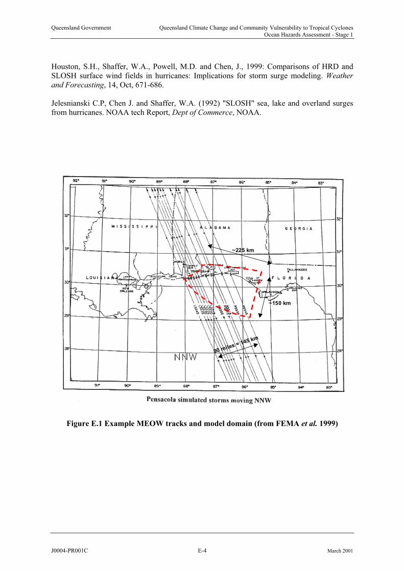
Queensland Government Queensland Climate Change and Community Vulnerability to Tropical CyclonesOcean Hazards Assessment - Stage 1
Houston, S.H., Shaffer, W.A., Powell, M.D. and Chen, J., 1999: Comparisons of HRD and SLOSH surface wind fields in hurricanes: Implications for storm surge modeling. Weather
and Forecasting, 14, Oct, 671-686.
Jelesnianski C.P, Chen J. and Shaffer, W.A. (1992) "SLOSH" sea, lake and overland surges from hurricanes. NOAA tech Report, Dept of Commerce, NOAA.
90 miles = 145 km
~150 km
~225 km
Figure E.1 Example MEOW tracks and model domain (from FEMA et al. 1999)
J0004-PR001C E-4 March 2001
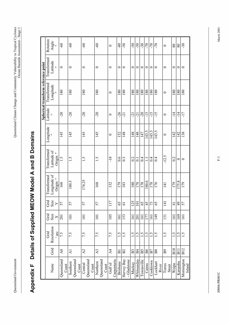
Quee
nsl
and G
over
nm
ent
Qu
een
slan
d C
lim
ate
Ch
ange
and
Co
mm
un
ity
Vuln
erab
ilit
y t
o T
rop
ical
Cy
clo
nes
Oce
an H
azar
ds
Ass
essm
ent
- S
tag
e 1
Ap
pe
nd
ix F
D
eta
ils
of
Su
pp
lie
d M
EO
W M
od
el
A a
nd
B D
om
ain
s
Sp
her
ical
tran
sform
ref
eren
ce p
oin
t
Nam
eG
rid
Gri
dR
esolu
tion
arc
Gri
dS
ize
X
Gri
dS
ize
Y
Tra
nsf
orm
edL
atit
ud
e o
fO
rig
inº
Longit
ude
ºL
atit
ud
eº
Tra
nsf
orm
edT
ran
sfo
rmed
Lat
itu
de
º
Ro
tati
on
Angle
º
Qu
een
slan
dC
oas
tA
07
.52
01
57
168
1.5
145
-20
180
0-6
0
Sou
ther
nQ
uee
nsl
and
Coas
t
A1
101
7.5
57
180
.51
.51
45
-20
180
0-6
0
Cen
tral
Qu
een
slan
dC
oas
t
A2
101
7.5
57
174
.25
1.5
145
-20
180
0-6
0
No
rth
ern
Qu
een
slan
dC
oas
t
A3
7.5
101
57
168
1.5
145
-20
180
0-6
0
Gu
lf o
f C
arp
enta
ria
A4
7.5
105
117
132
-18
00
00
0
Bri
sban
e1
.5B
11
61
65
179
0.6
152
-26
180
0-8
0
Her
vey
Bay
- G
lad
stone
B2
38
00
1.5
153
61
18
0.3
14
-21
18
0-5
Mac
kay
-21
B3
1.5
161
125
180
0.2
148
180
0-5
0
Wh
itsu
nd
ay1
88
0B
41
.52
01
01
17
0.1
14
-21
18
0-5
0
Tow
nsv
ille
B5
1.5
161
65
178
0.4
147
-20
180
0-3
0
Cai
rns
0B
61
.51
77
45
180
.61
.11
43
.5-1
51
80
-70
ook
tow
B7
1.5
161
178
0.4
143
.5-1
51
80
0-7
0
Lo
ckh
art
Riv
erB
80
1.5
149
65
176
0.4
143
.5-1
51
80
-70
To
rres
Str
ait
B9
1.5
131
141
141
-12
.50
00
00
Wei
pa
142
180
B1
01
.51
61
41
179
0.2
-14
08
0
Kar
um
ba
5B
11
1.
169
49
175
.80
142
-14
180
08
0
Mo
rnin
gto
nIs
land
B1
21
.51
61
57
179
01
38
-17
180
0-3
0
Tra
nsf
orm
edL
on
git
ud
e o
fO
rig
inº
Longit
ude
º
Cn
73
J0004-P
R001C
F-1
Mar
ch 2
00
1

Queensland Government Queensland Climate Change and Community Vulnerability to Tropical CyclonesOcean Hazards Assessment - Stage 1
Appendix G Recommended MEOW Technique for Storm Tide Forecasting
The following outlines the computational steps required to produce a MEOW forecast andaddresses the variety of methods which can be used in satisfying the data needs. The development here aims to preserve as much as possible the essential phase relationships inherent in the storm tide interaction, avoiding any simplifications which would otherwise dilute or destroy these elements. In the Australian context this is deemed to be an essential feature of an accurate MEOW forecast system.
G.1 Objective
The Maximum Envelope of Waters (MEOW) technique was originally outlined by Jarvinenand Lawrence (1985) as a robust storm tide forecast tool. The objective of the technique is to obtain the maximum forecast water level in a coastal domain due to the close approach and/or landfall of a tropical cyclone. Given that there is always uncertainty in any set of forecast storm parameters, the MEOW represents the prudent approach, or a "least regrets" philosophy, to try to ensure the safe evacuation of affected communities should that be required. On the other hand, forecasts should not be overly conservative to the extent that false alarms are excessive and the community is exposed to unnecessary evacuation risks and disruption, ultimately leading to complacency.
G.2 Background
The basic method has been in use by the US Weather Bureau for many years based on numerical simulations of storm surge using the SLOSH hydrodynamic model (Jelesnianski et
al. 1992). Guided by climatology, the SLOSH model is applied in a systematic manner to particular sections of coastline (e.g. FEMA et al. 1999), the various storm parameters are varied and the pre-computed storm surge results invoked during the forecasting process.Notwithstanding the basic philosophy, the actual technique can be implemented in a numberof different ways and the US approach involves significant simplifications in some areas which would not be applicable in Australia. For example, the tidal range is relatively low inthe Gulf of Mexico and accordingly the actual tide variation is merely approximated. Also, wave setup is excluded on the basis of the extensive shallow offshore regions. These latter approximations, together with further data reduction by the use of MOMS (MEOWS of MEOWS) may be the reason why there appears to be some present dissatisfaction with theUS warning system, leading to the perception that it is overly conservative (AMS 2000).
Besides its philosophical context, the "traditional" MEOW's principal advantage has been inovercoming the computational burden of utilising a sophisticated numerical simulation modelof storm surge in a real-time context. In the mid-1980s, for example, the computationaloverheads of real-time scenario testing of storm tide were prohibitive and a method which pre-computed these estimates was necessary. It also represented a considerable step forward relative to the manual nomogram technique based on the earlier SPLASH model (e.g. Nickerson 1971) not just in utility but also accuracy, since the nomogram methods relied onschematised rather than actual coastlines. The present study has also introduced the potential advantages of parametric methods as a way of reducing the data requirements of pre-computed MEOWs. Present computer capabilities are significantly greater now than when the method was introduced and fast approaching the capability to undertake multiple full scenariosimulations. However, the MEOW philosophy remains as the important forecast element,
J0004-PR001C G-1 March 2001

Queensland Government Queensland Climate Change and Community Vulnerability to Tropical CyclonesOcean Hazards Assessment - Stage 1
regardless of the data source being used. The following development therefore concentrateson the MEOW philosophy and comments where appropriate on differences in application depending on the various data sources which could be used.
G.3 Definitions
The following definitions set the scene for the development which follows. A generalisedcoastal site is considered where the resulting storm tide level over time will be a function ofthe relative phasing of each of the time-varying components of astronomical tide, imposedstorm surge and wave setup.
is the time varying storm tide level for any coastal site. Here is assumed constant for the duration of the storm tide event and is simply an offset to ensure the temporally local MWL is correctly matched. While there are some (generally) weak non-linearities in regard to overall water depth which influence both the tide and the storm surge these may be neglected initially. On the other hand, wave setup is a strong function of incident wave height, which is a function of water depth. To preserve this relationship, the following procedure ensures thatwave setup is calculated only after the tide and surge components are known.
The variation with time t of the normal astronomical tide (to AHD) at any coastal location is
described by [ ]t which may be modified by a local tidal anomaly due to background meteorological or other temporary influences not directly related to the incident storm tide.
The storm surge is described by [ ]t and the wave setup by [ ]t. The resulting storm tide level
[ ]t may then be considered (to first order accuracy) as the linear superposition of thesevarious time varying components, such that:
[ ]t = { + [ ]t + [ ]t } + [ ]t (G.1)
The maximum water level or MEOW is then of interest, together with the time of the maximum, e.g.
[ ]t=tmax = max ( [ ]t ) t=t1,t2 (G.2)
The MEOW can then be similarly applied across multiple sites, typically along a coastline or even as a 2-dimensional field of elevations if required.
G.4 Basic Methodology
The requirements needed to satisfy Eq (G.1) are now taken in order.
Tidal Anomaly
This is best obtained procedurally in real-time from the relevant State authority and based onactual monitoring of the tide at an appropriate open coast site during the immediate few days and/or hours. The difference between the predicted tide and the measured tide (the residual) over a finite period of record then provides the estimate of the tidal anomaly component. It may be negative or positive depending on the situation but will typically be less than 0.3 m. In the absence of real-time advice, pre-stored seasonal residuals derived from long term tidal analysis could be used as a base reference, assigned to the various Standard Ports (see below,
J0004-PR001C G-2 March 2001

Queensland Government Queensland Climate Change and Community Vulnerability to Tropical CyclonesOcean Hazards Assessment - Stage 1
State authorities should be consulted to determine the extent to which seasonal anomalies arealready included in the predicted tide and its published harmonic constituents).
Astronomical Tide [ ]t
This can be computed from a suitable set of harmonic constituents for each site and/or the most appropriate Standard Port in the circumstances. All available constituents should be used, subject to the advice of the relevant State authority, and harmonic reconstitution carried out in an appropriate manner (e.g. Foreman 1977). Resulting levels must be referred toAustralian Height Datum (AHD) and tidal plane information also recorded, especially HighestAstronomical Tide (HAT).
Tidal heights and planes at other sites should be based on published range and phase ratios relative to their Standard Port or interpolated appropriately as required to form a reference standard. Adjustment of heights and phases relative to the Standard Port should be done in accordance with advice from the relevant State authority.
Because the time of landfall and/or peak storm surge is not known apriori it remains to construct a vector of tide levels for each site spanning the period of interest (e.g. 24 h) whichmay then be combined with subsequent storm surge and wave setup time vectors. This can bedone efficiently in real-time.
Storm Surge [ ]t
We now acknowledge that storm surge is a complex function F of the nearshore10 incident
tropical cyclone parameters combined (implicitly here) with the localised bathymetry of the coastal site under consideration.
[ ] t = F [ p0, R, B, Vfm, fm, X, ... ] t (G.3)
where X represents the perpendicular distance of the storm centre from the site in question.For landfalling tracks X is taken as the perpendicular distance between the site and a straightline approximation of the track at the nominal "landfall" position. A positive X
indicates the site is located on the LHS of the storm. The "landfall" position is the intersection
of the straightline track and a line representing the coast, aligned at a bearing L relative tonorth (refer Figure G.1 for details). For near-parallel-coast tracks X is the closest approachdistance perpendicular to the straightline approximation to the track. The ellipses "..."indicates that the parameter dependence is likely subject to some variation, either due to developing knowledge of the best representation of these events, or due to local synoptic features and the like (e.g. associated ridging).
Initially, we consider the case of estimating [ ]t on the basis of simply the "best track"information, which will vary depending upon the particular data source being utilised, asfollows:
(a) Real-time numerical modellingIn this situation, a full scale hydrodynamic model (such as MMUSURGE) is invoked together with a representation of the site bathymetry, the tidal forcing and the surface wind and
10 Nearshore is taken here to imply within 6 to 12 h of landfall or closest approach.
J0004-PR001C G-3 March 2001
Queensland Government Queensland Climate Change and Community Vulnerability to Tropical CyclonesOcean Hazards Assessment - Stage 1
pressure field based on the forecast track parameters. Ideally the latter might be derived from a forecast product (e.g. TCLAPS) but more likely it will be a combination of a parametricwind and pressure field (e.g. Harper and Holland 1999) with merged forecast and/or
observation data. Using this approach, [ ]t will be obtained directly for all nominated sites,subject to sufficient forecast time being available to run the numerical model in real-time at the desired level of resolution. This direct method is more sensitive to equipment and/orsystems failure than (b) or (c) and requires much longer forecast lead times.
(b) Parametric storm surge modelling
This would be an analytic approximation to the site specific storm surge response derived from a series of pre-computed numerical storm surge model simulations (e.g. MMUSURGE
as above). The predicted [ ]t would be obtained by direct substitution of the forecast trackparameters into a site specific response function. The response functions would be derived using techniques similar to that below for the "traditional" MEOW database approach but not utilising the raw data directly. This method offers ease of direct application with very low computational needs but potentially sacrifices some degree of accuracy relative to (a).
(c) Traditional MEOW database
This would involve a real-time data recovery and (linear) interpolation of the forecast track parameters from, as per (b) above, a pre-computed set of discrete numerical model results for the region, i.e.
[ ]t = I [ p0p, R
r, B
b, X
x, Vfm
v, fm , ... ] t (G.4)
where I is an interpolation operator within the n-dimensional parameter space defined by the
range of discrete parameter values {p, r, b, x, v, , ...} obtained from a series of systematicnumerical model results. This method can become cumbersome in terms of on-line data and recovery requirements and is necessarily truncated by the available parameter space. It potentially represents comparable accuracy to (b) but with much greater system overheads.11
Combined Surge plus Tide Level [ ]t
The next step is to combine the [ ]t storm surge series with the corresponding tidal anomaly
and astronomical tide water levels [ ]t, the phasing of which will be dependent on thepredicted time of landfall tl, conceptually:
tl = ƒ [Vfm, fm] (G.5)
where ƒ incorporates the (pre-specified) geometric function describing the "coastline" for thepurpose of defining "landfall", or closest-approach, intersecting with the forecast vector storm
track dependent on the supplied track fixes (t, , )12.
11 The US approach here is to retain only maximum [ ]t and simplify by removing firstly the variation due to X
and then due to Vfm, fm to produce a MOM. This may result in significant loss of detail for Australian conditionswith highly variable coastal features and high tidal range.12 In the forecasting context the relative storm fixes and their variability in space at a given time is all that is
required to define this geometry. The forecast parameter variation in Vfm, fm is likewise calculated from the fix.
J0004-PR001C G-4 March 2001
Queensland Government Queensland Climate Change and Community Vulnerability to Tropical CyclonesOcean Hazards Assessment - Stage 1
The phase aligned surge plus tide water level sequence is then:
[ ] + [ ] ]t' = t'' + [ t' (G.6)
where t' indicates t phase-aligned at time tl.
Wave Setup [ ]t
Analogous to storm surge, wave setup is also a complex function f of the incident tropical
cyclone parameters combined with the localised bathymetry of the coastal site, but
additionally highly sensitive to stillwater level t'' i.e.
[ ]t'' = f [ p0, R, B, Vfm, fm, X, ... , ]t' (G.7)
Similarly, wave setup can be estimated by a range of data sources (a), (b) or (c) bysubstituting the hydrodynamic model with a spectral or other type of wave prediction model,for example, WAMGBR substituted for MMUSURGE.
Combined Storm Tide Level [ ]t
The total storm tide elevation time series is then:
[ ] ] ]
which is the original n-dimensional parameter space additionally with i=0,1,2,3,... for each of m parameter scenarios.
t' = [ t' + [ t' (G.8)
and the MEOW is accordingly given by Eq (G.2).
G.5 Incorporating Forecast Uncertainty
The above development is based on a single "best track" scenario which is now expanded within the MEOW philosophy to incorporate forecast parameter uncertainty. Within the multiple scenario forecast environment, the MEOW data source module must provide a range of, for example, storm surge levels for the site in question formed by the n × m-dimensionalparameter space e.g.
[ i]t = F [ p0i, Ri, Bi, Xi, Vfmi, fmi, ... ] t (G.9)
The multiple parameter cases are determined by expanding the specified forecast uncertainty
bounds of each parameter [ ] = { p0i, Ri, Bi, Xi, Vfmi, fmi, ...}, viz
i = 0 = expected or mean parameter value [ ]
1 = upper bound parameter value; say [ + i( )]
2 = lower bound parameter value; say [ - i( )] etc
where i( ) is the parameter error value having cumulative non-exceedance probability i( ).
J0004-PR001C G-5 March 2001

Queensland Government Queensland Climate Change and Community Vulnerability to Tropical CyclonesOcean Hazards Assessment - Stage 1
An example would be, say, for the uncertainty in forecast central pressure to be assumed to bedistributed normally about the mean and an estimate of the standard deviation alone used as the measure of parameter dispersion:
p0i i=0 940 expected pressure at landfall (hPa)
i=1 945 based on one standard deviation upper bound
[ 1(p01), 1(p01)] of [5.0 , 0.8413]
i=2 935 based on one standard deviation lower bound
[ 2(p02), 2(p02)] of [5.0 , 0.1587]
This can be extended to as many i ordinates as deemed necessary in describing the probability of non-exceedance function for that parameter. In practice, it is unlikely that more than 2 or 3 probability limits per parameter would be chosen but it may be desirable to include skewness(unequal upper and lower intervals etc) depending on the particular forecast trends. If the information can be related to climatology then a more detailed set of probability ordinatescould be used as the defaults.
The above is extended to include variability in regard to the time of landfall, thus providing a range of phase alignments with the storm surge, as well as wave setup. The MEOW at a single site then becomes:
[ i]t=tmax = max { ( [ i]t ) t=t1,t2} i=0,m (G.10)
Assuming independence of each parameter uncertainty, the marginal probability of each scenario is then retained and accumulated as , the multiplicative sum of each component probability, such that:
Prob [ i]t=tmax = { i( i) } i=0,m (G.11)
Graphing of { [ i]t=tmax versus Prob[ i]t=tmax } will then permit consideration of the probabilistic variability in the storm tide predictions, for example, the extent to which theMEOW is more or less likely than a range of other water levels on that day. This will enable a degree of judgement to be exercised in addition to the single MEOW level being forecast for a site.
G.6 References
AMS (2000) Policy issues in hurricane preparedness and response. Proc of The Weather Channel Forum, Developed by the Atmospheric Policy Program of the American
Meteorological Society, Sept.
FEMA et al. (1999) Northwest Florida hurricane evacuation study. Prep by FEMA, NOAA,
State of Florida and US Army Corps of Engineers, July.
Foreman M.G.G. (1977) Manual for tidal heights analysis and prediction. Report 77-10, Institute of Ocean Sciences, Patricia Bay.
J0004-PR001C G-6 March 2001
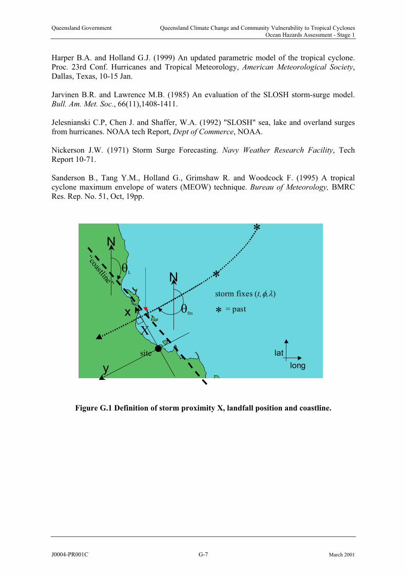
Queensland Government Queensland Climate Change and Community Vulnerability to Tropical CyclonesOcean Hazards Assessment - Stage 1
Harper B.A. and Holland G.J. (1999) An updated parametric model of the tropical cyclone. Proc. 23rd Conf. Hurricanes and Tropical Meteorology, American Meteorological Society,Dallas, Texas, 10-15 Jan.
Jarvinen B.R. and Lawrence M.B. (1985) An evaluation of the SLOSH storm-surge model.Bull. Am. Met. Soc., 66(11),1408-1411.
Jelesnianski C.P, Chen J. and Shaffer, W.A. (1992) "SLOSH" sea, lake and overland surges from hurricanes. NOAA tech Report, Dept of Commerce, NOAA.
Nickerson J.W. (1971) Storm Surge Forecasting. Navy Weather Research Facility, Tech Report 10-71.
Sanderson B., Tang Y.M., Holland G., Grimshaw R. and Woodcock F. (1995) A tropicalcyclone maximum envelope of waters (MEOW) technique. Bureau of Meteorology, BMRC Res. Rep. No. 51, Oct, 19pp.
Figure G.1 Definition of storm proximity X, landfall position and coastline.
+
++ = forecast
nominal
“landfall”L
N
fm
*
*
storm fixes (t, , )
* = past“coastline”
site
x
y
N
long
lat
X
J0004-PR001C G-7 March 2001

Queensland Government Queensland Climate Change and Community Vulnerability to Tropical CyclonesOcean Hazards Assessment - Stage 1
Appendix H MEOW Database Requirements and Storage Costs
This appendix addresses workscope Item A-4 and is based on the development of MEOWdata generation scenarios in Section 11.5.
H.1 Storage Requirements and Indicative Costs
The "desirable" Scenario 2 suggests order-of-magnitude data storage would be 550 GB for aB grid resolution 24 h duration MEOW for the whole Queensland coast, storing only data within 10 grid points of the shore. If all data points were to be stored this would increase to the order of 7000 GB.
DAT facility $10000
Whilst the data storage even for the recommended 550 GB case is non-trivial, the data relationships are relatively simple and information retrieval is unlikely to rely on the use of a complex database system (refer next section). Nevertheless, it may be more convenient to simply adopt Bureau of Meteorology standard (e.g. netCDF™ or Oracle™) interfaces and post-process the surge model data to suit. It is not presently possible to estimate whether thispost-processing activity itself might represent any significant CPU requirement.
Notwithstanding the above, not all of the 550 GB of data would be required at any one timeand only the data sets specifically relevant to the forecast problem need be retrieved from an archive storage medium (e.g. DAT tape or DVD). This could reduce the online data requirements to the order of 150 GB or possibly less, assuming a target domain and the two adjacent domains' data were to be retrieved. Hence, assuming off-line storage requirementsare of the order of 500 GB, present readily available DAT technology of 40 GB/tape would require only 12 tapes but with (say) 2 backup copies, totalling 36 tapes. Retrieval time of the500 GB would be approximately 1 days at 20 GB/h. Assuming the online requirement at any one time is only 150 GB, retrieval time would be less than 7 h to establish the immediatedomain requirements. Online storage would be by (say) 40 GB SCSI HDD, requiring 4 in total.
Assuming a dedicated workstation is desirable for operational purposes, the following hardware costs are indicative:
Base workstation $ 5000
HDD online $10000Total: $25000
Duplication of at least the DAT facility and HDD storage (e.g. RAID) would also berecommended for operational purposes, yielding an overall facility capital expenditure of theorder of $50000. The DAT archive would require ongoing maintenance throughout its life, probably requiring transfer to DVD at some future time to preserve data quality. As noted inSection 11.5, it is likely a dedicated Bureau officer would also be required to oversee the production.
An alternative to the above "in-house" production option would be to seek external supply under contract, which would ensure Bureau resources are not diminished during this phase.
J0004-PR001C H-1 March 2001

Queensland Government Queensland Climate Change and Community Vulnerability to Tropical CyclonesOcean Hazards Assessment - Stage 1
H.2 Suggested Data Base Structure
It is recommended that MEOW data sets be retained as a simple series of flat data files,identified by a systematic filenaming convention. Each model simulation will represent the result of a given set of MEOW parameters for a particular domain. Each set of results can then logically be retained in a directory with the domain name as the principal or key "data base" identifier.
Each MEOW file will need to retain a timeseries of "snapshots" of (time-stamped) waterlevels covering the output sub-set of the domain (i.e. within 10 grid points of shore) at the chosen space and time resolution. For B grids this will be 2.8 km and a chosen multiple of900 s, say 1800 s.
It is proposed that a unique filename be constructed based on the point estimates of the various parameters describing each simulation, viz
The parameters envisaged (as per Appendix G) are:
p0 central pressure (or pressure deficit) hPap
R radius to maximum winds kmr
B b wind field peakedness -
X distance from target km x
V forward speed m sfm v
track bearingfm' wind field asymmetry (if adopted) max
The resulting filename would then be, for example,:
p_r_b_x_v_ _ '.meow
where each of the above (p,r,b, etc) would be substituted by the specific point parameter used.
A typical path and filename under these rules might be:
Hervey_Bay/40_30_1_100_2_180_65.meow
Alternatively, each parameter point value could be allocated a simple index (1,2,3 etc) and thefilename again concatenated in the same sequence, e.g.
Hervey_Bay/2_2_1_4_1_9_1.meow
where the first index (2) refers to the 2nd point value of p for the Hervey Bay domain.
The latter naming method would facilitate name generation and retrieval whereas the formerwould suit visual identification.
To reconstruct the MEOW forecast, as described in Appendix G, a number of data files would need to be retrieved and the time series of stored data overlaid with tidal data to construct theactual MEOW forecast.
-1
J0004-PR001C H-2 March 2001