Observations of Turbulence Caused by a Combination of Tides and MeanBaroclinic Flow over a Fjord Sill

ANDRE STAALSTRØM

Section for Biogeochemistry and Physical Oceanography, Norwegian Institute for Water Research, and

Department of Geosciences, University of Oslo, Oslo, Norway

LARS ARNEBORG AND BENGT LILJEBLADH

Department of Earth Sciences, University of Gothenburg, Gothenburg, Sweden

GÖRAN BROSTRÖM

Department of Earth Sciences, University of Gothenburg, Gothenburg, Sweden, and Division for

Oceanography and Marine Meteorology, Norwegian Meteorological Institute, Oslo, Norway

(Manuscript received 13 September 2013, in final form 23 September 2014)

ABSTRACT

This study investigates the dissipation rates and flow conditions at theDrøbak Sill in theOslofjord. The areawas transected 13 times with a free-falling microstructure shear probe during 4 days in June 2011. At the sametime, an ADCP was deployed inside the sill. During most tidal cycles, internal hydraulic jumps with highdissipation rates were found on the downstream side of the sill. However, the internal response varied stronglybetween different tidal cycles with similar barotropic forcing. In the beginning of the observational period, ebbtides had no hydraulic jumps, and in the end one of the flood tides did not have a hydraulic jump. During thesame period, the mean baroclinic exchange flow changed from inflow to outflow in the bottom layer. Theauthors conclude that the conditions at the sill are on the edge of forming hydraulic jumps and that the meanbaroclinic exchange may push the flow above or below the limit of a hydraulic jump depending on the situ-ation. This conclusion is supported by two-layer hydraulic theory. The volume-integrated dissipation rateswithin 500m from the sill crest compare well with estimates of energy loss in the lower layer calculated from

the Bernoulli drop under the assumption of no energy loss in the upper layer. Finally, the mean dissipation

rate at the sill was compared with the radiation of internal tidal energy away from the sill, and it was found that

about 60%–90% of the total energy loss was dissipated locally.

1. Introduction

Flow–topography interactions caused by stratified flow

over, around, and through rough topography are impor-

tant for mixing in the deep abyssal ocean (e.g., Ledwell

et al. 2000), over the shelf (e.g., Nash andMoum2001), and

in fjords (e.g., Arneborg and Liljebladh 2009). Fjord en-

trances with sills are typical locations of strong flow–

topography interactions due to strong barotropic and

baroclinic currents caused by tides and exchange processes

between the fjord and the coastal water (e.g., Arneborg

2004). Barotropic tides can lose energy to turbulence

locally at the sill through bottom friction, formation of

downstream jets with separation from the sides, and

through formation of internal hydraulic jumps. They can

also lose energy to internal tides, internal lee waves, and

other internal waves that may propagate away and

transfer energy to turbulence and mixing elsewhere

(e.g., Klymak and Gregg 2004; Inall et al. 2005). Al-

though detailed studies have been performed in some

fjords, knowledge is still missing about when different

processes are important and how much mixing they

cause and where. The feature that can be most suc-

cessfully modeled is probably the internal tide genera-

tion, where simple two-layer (Stigebrandt 1976, 1999) or

Denotes Open Access content.

Corresponding author address: Andre Staalstrøm, Norwegian In-stitute for Water Research, Gaustadalleen 21, 0349 Oslo, Norway.E-mail: ans@niva.no

FEBRUARY 2015 S TAAL STRØM ET AL . 355

DOI: 10.1175/JPO-D-13-0200.1

� 2015 American Meteorological Society

continuous stratification (Stacey 1984) models tend to

give results of the correct order of magnitude for the

energy propagation into fjords (e.g., Stacey 1984; Klymak

and Gregg 2004; Arneborg and Liljebladh 2009).

Stigebrandt and Aure (1989) proposed that the baro-

tropic energy loss at the sill is dominated by internal

tide generation when the Froude number

Fr5 ys/c1 (1)

is less than one (so-called wave fjords) and that jets

dominate for Fr . 1 (jet fjords). Here, ys is the baro-

tropic tidal velocity amplitude over the sill, and c1 is the

phase speed of the first internal wave mode in the deep

water away from the sill. However, observations in-

dicate that both the local energy loss at the sill and in-

ternal tide generation are important for Fr ranging from

small values (Arneborg and Liljebladh 2009) to values

close to and above one (Klymak and Gregg 2004; Inall

et al. 2005). Stashchuk et al. (2007) reveal strong baro-

clinic wave response in the Scottish Loch Etive, where

Fr is much higher than 1 at the sill crest, and it is shown

that the origin of these waves is at a deeper part of the

sill, away from the sill crest, where Fr is less than one.

However, note that Fr 5 1 is not a good indication for

critical conditions at the sill, since the internal wave

velocity is not given by c1 in the presence of strong shear

and local depth changes over the sill that are caused by

nonlinearity of the flow.

A more relevant Froude number for two-layer flow is

the composite Froude number (e.g., Farmer andDenton

1985) defined as

G25Fr21 1Fr22 , (2)

where

Fr2i 5r2

r2 2 r1

y2ighi

, i5 1, 2. (3)

The ri are the densities, yi are the velocities, hi are the

thicknesses for the upper (i5 1) and lower (i5 2) layers,

and g is the gravitational acceleration. Under the as-

sumption of a rigid lid at the surface, the propagation

speed of one of the two long internal wave solutions

vanishes when G2 5 1, which is called critical flow. This

means that long internal waves can propagate in both

directions for G2 , 1 (subcritical flow), while they can

only travel in one direction for G2 . 1 (supercritical

flow). Then, if the fjord width is constant, the flow can

only change smoothly from subcritical to supercritical

conditions when the bottom slope is zero, for example,

at the sill crest, where it is then said to be hydraulically

controlled (e.g., Armi 1986). Hydraulic jumps occur

when the flow over the sill is strong enough to create

controlled flow at the sill, thus the supercritical flow on

one side of the sill must somehow adjust to the sub-

critical flow further away from the sill, which happens in

a dissipative jump (Fig. 1) (e.g., Baines 1995).

Tidal flow is not steady, but if the tidal particle orbit

ys/v, where v is the angular frequency of the tide, is long

compared with the length scale L, we may assume that

the steady hydraulic theory gives reasonable predictions

of some basic features of the flow. In Knight Inlet, the

observed jump tends to develop slower than predicted

by two-dimensional primitive equation model results,

where the flow causes an internal lee wave that quickly

breaks (Cummins 2000). The observed slow response was

first explained by the importance of flow separation and

small-scale entrainment for flow development (Farmer

and Armi 1999; Cummins 2000). Later it was argued

(Afanasyev and Peltier 2001; Klymak and Gregg 2001,

2003) that three-dimensional effects and a downstream

density pool rather than small-scale processes could ex-

plain the differences between observations and models.

If baroclinic mean currents are superposed on the

barotropic tides, this may be expected to influence the

occurrence of critical conditions at the sill. For two-layer

flow over a sill, which is subcritical upstream of the sill,

only the bottom layer will be accelerated over the sill

crest and dominate G there (e.g., Armi 1986). There-

fore, one may assume that a baroclinic mean current in

the bottom layer will tend to increaseG when it is in the

same direction as the tidal orbital velocity and decrease

G during the rest of the tidal phases.

In the present work, we analyze detailed microstruc-

ture transects through internal hydraulic jumps at the

Drøbak Sill of theOslofjord. TheDrøbak Sill with a depthof 20m is the main sill of the Oslofjord, separating the

150-m-deep inner basins from the deep outer parts of the

fjord (Fig. 2). Although the tides are relatively weak

FIG. 1. Sketch of a hydraulically controlled two-layer flow over

a sill. The flow is from left to right. The horizontal length scale of

the sill is L. The vertical drop in the interface is Dh.

356 JOURNAL OF PHYS ICAL OCEANOGRAPHY VOLUME 45

(’0.15-m semidiurnal tidal amplitude), the barotropic

current amplitude over the sill is about ys 5 0.4m s21.

With a mode-1 phase speed of about c1 5 0.9m s21

(Staalstrøm et al. 2012), the resulting Froude number

Fr’ 0.45 is well below one implyingwave–fjord conditions

as defined by Stigebrandt and Aure (1989). Nevertheless,

we observe hydraulic jumps in this study. In comparison,

the Froude numbers are Fr ’ 0.75 in Knight Inlet

(Stigebrandt 1999) and Fr’ 1.8 in Loch Etive (Inall et al.

2004). The length scale of the Drøbak Sill is about 500m,

which is much less than the tidal orbital amplitude (ys/v’2900m), and we expect quasi-steady hydraulic theory to

be valid over this sill.

The main focus of the present study is to investigate

the structure of internal hydraulic jumps and associated

dissipation rates of turbulent kinetic energy over the

Drøbak Sill, the partition of the barotropic energy loss atthe sill, and how mean baroclinic currents over the sill

FIG. 2. (a) Map of the Oslofjord. The black dot is the meteorological station Gulholmen. (b) Map of the area around the Drøbak Sill.White circles are the ADCP moorings. MSS stations are marked with black dots. Sea level is recorded at station Oscarsborg (OSC; whitecircle) operated by the Norwegian Hydrological Survey. The area 500m north and south of the Drøbak Sill is our focus area and is indicatedwith red lines, and the coordinate system used in the calculations is indicated with green arrows. Bathymetric data are from the GeologicalSurvey of Norway (Lepland et al. 2009). A grayscale indicates the depths down to 130m. A hillside shade effect is used to emphasize the

bathymetric structure. The subsurface Drøbak Jetty runs from Kaholmen south (KaS) to Småskjær (Sm) and further to the mainland on thewest sideof the sound and ismarkedwith a red dashed line. TheDrøbak Sill (20m) is located between Småskjær andDrøbak. There is a secondsill (47m) between Kaholmen north (KaN) and the southern tip of Hallangstangen, marked with a red dashed line.

FEBRUARY 2015 S TAAL STRØM ET AL . 357

influence the hydraulic jumps. The instrument setup andthe principle behind calculations of the dissipation rateare briefly described in section 2. In section 3, we presentthe data, starting with ADCP data and repeated mi-

crostructure transects over the sill from June 2011,

continuing with examples of ADCP data at the sill from

2009. We then present estimates of integrated dissipa-

tion rates in the sill region, estimates of energy loss in the

lower layer based on the Bernoulli function, and com-

parison with the velocity in the lower layer at the sill.

Finally, the results are discussed in section 4.

2. Methods

a. Dataset

In this paper, we present a combination of observa-

tions of currents at fixed positions and vertical profiles of

stratification and dissipation rates of turbulent kinetic

energy along transects. The data were mainly collected

during the period 20 to 23 June 2011 on board the Re-

search Vessel (R/V) Trygve Braarud. The wind condi-

tions were relatively calm during the data collection.

The maximum measured wind speed at station

Gullholmen (59826.110N, 10834.680E) was 8.4m s21. A

microstructure shear profiler (MSS90L, hereinafter

MSS) was dropped continuously from the stern of the

ship as it cruised at low speeds (’1 kt). The MSS90L is

a loosely tethered profiler with standard conductivity,

temperature, and pressure (CTD) sensors as well as two

airfoil shear probes (PNS06) sampling at 1024Hz, while

the profiler is descending vertically with a speed of 0.6–

0.7m s21. A more detailed discussion of an earlier ver-

sion of the instrument can be found in Prandke and Stips

(1998). A sensor protection guard allows profiling down

to the bottom (with sensors 0.1m above bottom). The

data from the upper 2–3m that were influenced by vessel

turbulence was removed. A total of 15 transects were

performed; 13 along-fjord transects over the Drøbak Silland 2 across-fjord transects just inside the sill. Alto-gether we collected 368 profiles, and the positions ofthese profiles are shown as black dots in Fig. 2. The times

of the transects are indicated in Fig. 3a as gray bars on

top of the sea level (SL) measured at Oscarsborg.

An upward-looking acoustic Doppler current profiler

(ADCP; Nortek Continental 190 kHz) was deployed at

100-m depth at station S2 (59840.670N, 10836.710E) be-fore the first MSS transect in 2011 and recovered after

the last transect. The current profiler provided reliable

data between 10.5- and 94.5-m depths with a resolution

of 3m in depth and 10min in time.

We also utilize two ADCP datasets from September

2009, when upward-looking ADCPs were deployed at

station S1 (RDI600) and at station S2 (Nortek Continental

190kHz). The ADCP at station S1 (59840.080N,

10836.940E) was deployed at the bottom just inside the

sill crest at 23-m depth. The vertical resolution was 1m

between 2.5- and 21.5-m depths. At station S2 the setup

was the same as in 2011.

b. Analyses

Dissipation rates of turbulent kinetic energy were

obtained from the microstructure shear data using

standard methods, as described in more detail by, for

example, Arneborg and Liljebladh (2009). The shear

probes measure how one transverse velocity component

changes along the path of the profiler. From the shear

variance, one can calculate the dissipation rate under the

assumption of isotropic turbulence. However, since the

sensors do not cover the complete wavenumber range of

the shear variance, the dissipation rates are obtained

by fitting the observed shear spectrum to the universal

Nasmyth spectrum for that component. This is done in 50%

overlapping 512-point segments, and the resulting esti-

mates of the dissipation rate are averaged into 1-m bins.

In the present case, the main problem with this

method is that the velocity of the sensor tip through the

water is estimated from the rate of change of the pres-

sure. The velocity through the water enters the calcu-

lation of dissipation rates to the power of 4, so small

errors in the velocity give considerable errors in the

dissipation rate. As discussed in Klymak and Gregg

(2004), this may cause a large problem in a hydraulic

jump where the vertical velocities can be large relative

to the sinking velocity of the profiler. As proposed by

Klymak and Gregg (2004), we also considered a con-

stant velocity rather than that calculated from the

pressure. However, except for one extreme case with

small fall velocity (0.3m s21) near the bottom, which was

removed, we found no large differences doing this

(,15% in integrated dissipation). Considering that the

fall velocity may also be influenced by other effects, for

example, strong shear and density changes, we did not

find it justifiable to use anything else than the standard

method in this case.

3. Results

In this section, we will first present results from the

moored instruments at station S2, followed by results

from the dissipation measurements. Based on these

data, we present current measurements at the sill from

2009 and both composite and layerwise Froude number

estimates. Finally, we integrate the dissipation rates and

compare the total dissipation rates with the energy loss

in the lower layer estimated fromBernoulli drops. In the

following all times are local times (UTC 1 2 h).

358 JOURNAL OF PHYS ICAL OCEANOGRAPHY VOLUME 45

a. Mooring data at S2 in 2011

During the field study, the sea level variations were

dominated by a semidiurnal tidal signal with a range of

about 0.3m superposed by a higher harmonic (Fig. 3a).

It has earlier been found that the shape of the tidal

curve in the Oslofjord is well described by the sum of

a semidiurnal and a quarter-diurnal tidal constituent

(Tryggestad 1974). This is often seen as two distinct

maxima during the flood current (cf. Fig. 3b) at station

S2 inside the Drøbak Sill. It is also notable that the floodcurrents are generally strong (up to about 0.5ms21 at

S2) and concentrated in the depth range of 15–30m in-

side the sill (which is around the sill depth of 20m), while

the ebb currents are weaker and much more uniformly

distributed in depth.

The subtidal velocities in the observed depth range

(below 10.5m) are positive into the fjord in the begin-

ning of the observation period and negative in the end of

the period. The barotropic velocities corresponding to

the observed detided sea level variations (Fig. 3a) are

less than 1 cm s21, which is much less than the observed

tidal velocities. The observed velocities must therefore

be a baroclinic flow with oppositely directed flow in the

FIG. 3. (a) SL measured by the Hydrographic Service of the Norwegian Mapping Authority

at the tide gauge station of Oscarsborg (Fig. 2) plotted with a bold black line and the estimated

flow in the lower layer over the sill y2 in bold red. The mean sea level and mean flow, con-

structed by taking the running mean over a tidal period, is plotted as thin lines, in black and red,

respectively. EachMSS transect ismarkedwith gray shading. (b)Observed current along the fjord

at station S2. The color scale indicates current speed inms21. Red colors indicate currents into the

fjord (flood) and blue out of the fjord (ebb). (c) Estimated composite and layerwise Froude

numbers at the sill based on current and sea level measurements at station S2. The gray shading

indicates the error range for G2. (d) Integrated dissipation based on direct measurements (gray

bars) and estimated from (6) (red line). The pink shading indicates the error range for Eemp.

FEBRUARY 2015 S TAAL STRØM ET AL . 359

two layers (above and below 10.5m). These kind of fluc-

tuating baroclinic currents are commonly seen in the fjords

around Skagerrak (e.g., Aure et al. 1996; Arneborg 2004).

b. MSS transects

MSS transects over the sill were taken during six

subsequent flood tides (transects 1, 2, 3, 6, 7, 9, 14, and

15) and during two ebb tides (transects 4, 5, 10, 11, 12,

and 13), as indicated with gray shading in Fig. 3a.

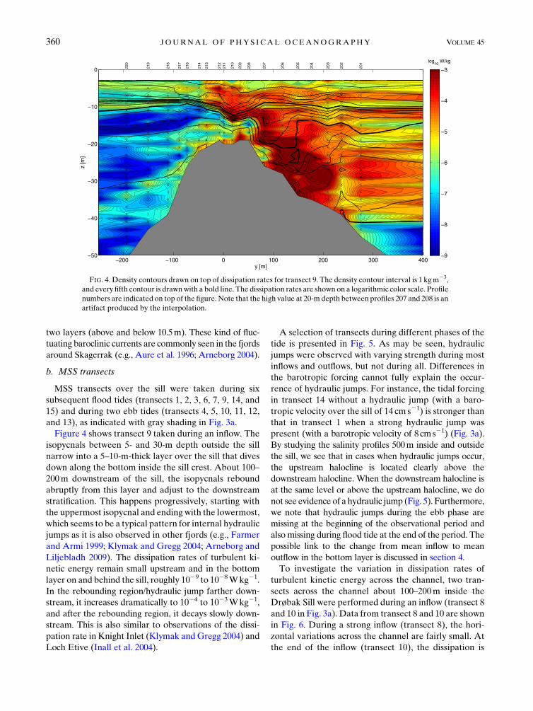
Figure 4 shows transect 9 taken during an inflow. The

isopycnals between 5- and 30-m depth outside the sill

narrow into a 5–10-m-thick layer over the sill that dives

down along the bottom inside the sill crest. About 100–

200m downstream of the sill, the isopycnals rebound

abruptly from this layer and adjust to the downstream

stratification. This happens progressively, starting with

the uppermost isopycnal and ending with the lowermost,

which seems to be a typical pattern for internal hydraulic

jumps as it is also observed in other fjords (e.g., Farmer

and Armi 1999; Klymak and Gregg 2004; Arneborg and

Liljebladh 2009). The dissipation rates of turbulent ki-

netic energy remain small upstream and in the bottom

layer on and behind the sill, roughly 1029 to 1028Wkg21.

In the rebounding region/hydraulic jump farther down-

stream, it increases dramatically to 1024 to 1023Wkg21,

and after the rebounding region, it decays slowly down-

stream. This is also similar to observations of the dissi-

pation rate in Knight Inlet (Klymak and Gregg 2004) and

Loch Etive (Inall et al. 2004).

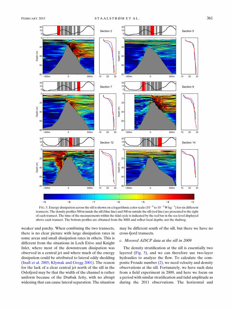
A selection of transects during different phases of the

tide is presented in Fig. 5. As may be seen, hydraulic

jumps were observed with varying strength during most

inflows and outflows, but not during all. Differences in

the barotropic forcing cannot fully explain the occur-

rence of hydraulic jumps. For instance, the tidal forcing

in transect 14 without a hydraulic jump (with a baro-

tropic velocity over the sill of 14 cm s21) is stronger than

that in transect 1 when a strong hydraulic jump was

present (with a barotropic velocity of 8 cms21) (Fig. 3a).

By studying the salinity profiles 500m inside and outside

the sill, we see that in cases when hydraulic jumps occur,

the upstream halocline is located clearly above the

downstream halocline. When the downstream halocline is

at the same level or above the upstream halocline, we do

not see evidence of a hydraulic jump (Fig. 5). Furthermore,

we note that hydraulic jumps during the ebb phase are

missing at the beginning of the observational period and

also missing during flood tide at the end of the period. The

possible link to the change from mean inflow to mean

outflow in the bottom layer is discussed in section 4.

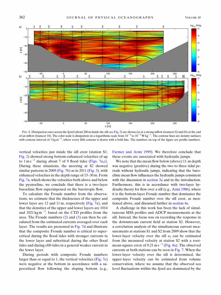
To investigate the variation in dissipation rates of

turbulent kinetic energy across the channel, two tran-

sects across the channel about 100–200m inside the

Drøbak Sill were performed during an inflow (transect 8and 10 in Fig. 3a). Data from transect 8 and 10 are shown

in Fig. 6. During a strong inflow (transect 8), the hori-

zontal variations across the channel are fairly small. At

the end of the inflow (transect 10), the dissipation is

FIG. 4. Density contours drawn on top of dissipation rates for transect 9. The density contour interval is 1 kgm23,

and every fifth contour is drawnwith a bold line. The dissipation rates are shown on a logarithmic color scale. Profile

numbers are indicated on top of the figure. Note that the high value at 20-m depth between profiles 207 and 208 is an

artifact produced by the interpolation.

360 JOURNAL OF PHYS ICAL OCEANOGRAPHY VOLUME 45

weaker and patchy. When combining the two transects,

there is no clear picture with large dissipation rates in

some areas and small dissipation rates in others. This is

different from the situations in Loch Etive and Knight

Inlet, where most of the downstream dissipation was

observed in a central jet and where much of the energy

dissipation could be attributed to lateral eddy shedding

(Inall et al. 2005; Klymak and Gregg 2001). The reason

for the lack of a clear central jet north of the sill in the

Oslofjord may be that the width of the channel is rather

uniform because of the Drøbak Jetty, with no abruptwidening that can cause lateral separation. The situation

may be different south of the sill, but there we have nocross-fjord transects.

c. Moored ADCP data at the sill in 2009

The density stratification at the sill is essentially two

layered (Fig. 5), and we can therefore use two-layer

hydraulics to analyze the flow. To calculate the com-

posite Froude number (2), we need velocity and density

observations at the sill. Fortunately, we have such data

from a field experiment in 2009, and here we focus on

a period with similar stratification and tidal amplitude as

during the 2011 observations. The horizontal and

FIG. 5. Energy dissipation across the sill is shown on a logarithmic color scale (1029 to 1023Wkg21) for six different

transects. The density profiles 500m inside the sill (blue line) and 500moutside the sill (red line) are presented to the right

of each transect. The time of the measurements within the tidal cycle is indicated by the red bar in the sea level displayed

above each transect. The bottom profiles are obtained from the MSS and reflect local depths, not the thalweg.

FEBRUARY 2015 S TAAL STRØM ET AL . 361

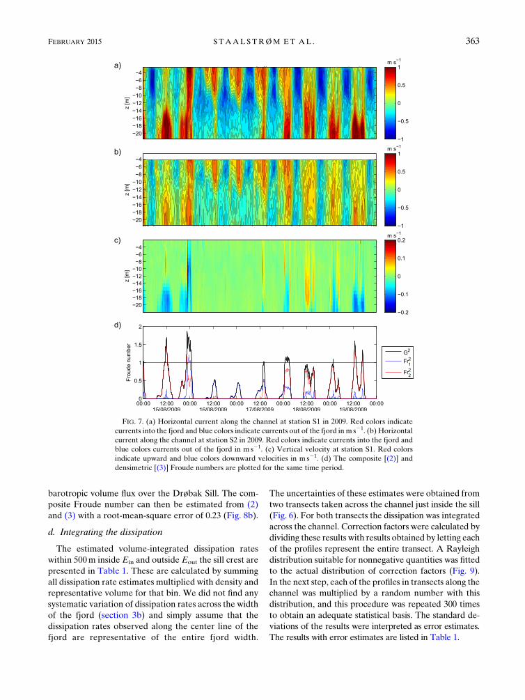
vertical velocities just inside the sill crest (station S1;

Fig. 2) showed strong bottom-enhanced velocities of up

to 1m s21 during about 7 of 9 flood tides (Figs. 7a,c).

During these situations, the mooring at S2 showed

similar patterns in 2009 (Fig. 7b) as in 2011 (Fig. 3), with

enhanced velocities in the depth range of 15–30m. From

Fig. 7a, which shows the velocities both above and below

the pycnocline, we conclude that there is a two-layer

baroclinic flow superimposed on the barotropic flow.

To calculate the Froude number from the observa-

tions, we estimate that the thicknesses of the upper and

lower layer are 12 and 11m, respectively (Fig. 7a), and

that the densities of the upper and lower layers are 1014

and 1021 kgm23, based on the CTD profiles from the

area. The Froude numbers (2) and (3) can then be cal-

culated from the estimated currents averaged over each

layer. The results are presented in Fig. 7d and illustrate

that the composite Froude number is critical to super-

critical during the flood tides with stronger currents in

the lower layer and subcritical during the other flood

tides and during ebb tides in a general weaker current in

the lower layer.

During periods with composite Froude numbers

larger than or equal to 1, the vertical velocities (Fig. 7c)

were negative at the bottom in accordance with a su-

percritical flow following the sloping bottom (e.g.,

Farmer and Armi 1999). We therefore conclude that

these events are associated with hydraulic jumps.

We note that themean flow below (above) 11-m depth

was negative (positive) during the two to three tidal pe-

riods without hydraulic jumps, indicating that the baro-

clinic mean flow influences the hydraulic jumps consistent

with the discussion in section 3a and in the introduction.

Furthermore, this is in accordance with two-layer hy-

draulic theory for flow over a sill (e.g., Armi 1986), where

it is the bottom-layer Froude number that dominates the

composite Froude number over the sill crest, as men-

tioned above, and discussed further in section 4a.

A challenge in this work has been the lack of simul-

taneous MSS profiles and ADCP measurements at the

sill. Instead, the focus was on recording the response in

the downstream current field at station S2. However,

a correlation analysis of the simultaneous current mea-

surements at stations S1 and S2 from 2009 show that the

lower-layer velocity over the sill y2 can be estimated

from the measured velocity at station S2 with a root-

mean-square error of 0.21m s21 (Fig. 8a). The observed

currents at both stations can be seen in Fig. 7. When the

lower-layer velocity over the sill is determined, the

upper-layer velocity can be estimated from volume

conservation, where we assume that the observed sea

level fluctuations within the fjord are dominated by the

FIG. 6. Dissipation rates across the fjord (about 200m inside the sill; see Fig. 2) are shown (a) at a strong inflow (transect 8) and (b) at the end

of an inflow (transect 10). The color scale is dissipation on a logarithmic scale from 1029 to 1023Wkg21. The contour lines are density surfaces

with contour interval of 1kgm23, where every fifth contour is drawn with a bold line. The numbers on top of the figure are profile numbers.

362 JOURNAL OF PHYS ICAL OCEANOGRAPHY VOLUME 45

barotropic volume flux over the Drøbak Sill. The com-posite Froude number can then be estimated from (2)

and (3) with a root-mean-square error of 0.23 (Fig. 8b).

d. Integrating the dissipation

The estimated volume-integrated dissipation rates

within 500m inside Ein and outside Eout the sill crest are

presented in Table 1. These are calculated by summing

all dissipation rate estimates multiplied with density and

representative volume for that bin. We did not find any

systematic variation of dissipation rates across the width

of the fjord (section 3b) and simply assume that the

dissipation rates observed along the center line of the

fjord are representative of the entire fjord width.

The uncertainties of these estimates were obtained from

two transects taken across the channel just inside the sill

(Fig. 6). For both transects the dissipation was integrated

across the channel. Correction factors were calculated by

dividing these results with results obtained by letting each

of the profiles represent the entire transect. A Rayleigh

distribution suitable for nonnegative quantities was fitted

to the actual distribution of correction factors (Fig. 9).

In the next step, each of the profiles in transects along the

channel was multiplied by a random number with this

distribution, and this procedure was repeated 300 times

to obtain an adequate statistical basis. The standard de-

viations of the results were interpreted as error estimates.

The results with error estimates are listed in Table 1.

FIG. 7. (a) Horizontal current along the channel at station S1 in 2009. Red colors indicate

currents into the fjord and blue colors indicate currents out of the fjord in m s21. (b) Horizontal

current along the channel at station S2 in 2009. Red colors indicate currents into the fjord and

blue colors currents out of the fjord in m s21. (c) Vertical velocity at station S1. Red colors

indicate upward and blue colors downward velocities in m s21. (d) The composite [(2)] and

densimetric [(3)] Froude numbers are plotted for the same time period.

FEBRUARY 2015 S TAAL STRØM ET AL . 363

Inside the sill, the highest value was 3500 6 1500 kW,

the lowest value was 2.7 6 0.8 kW, and the mean value

was 6606 290 kW. At the outside, the largest value was

1500 6 560 kW, the lowest value was 1.9 6 0.6 kW, and

the mean value was 160 6 64 kW. The high value of

Eout was obtained during the only observed hydraulic

jump outside the sill (transect 12). The Froude num-

bers, estimated as described in section 3c, are drawn as

a time series (Fig. 3c) above the results from Table 1

(Fig. 3d), and it is evident that in the cases where Ein

exceeds about 3000kW it is probable that we haveG2. 1.

However, inaccuracy in the estimate of G2 leaves

some uncertainty whether or not the value actually

exceeds 1. The cases with very high values of in-

tegrated dissipation rates are all obtained during the

presence of hydraulic jumps, which dominate the es-

timates of the mean dissipation rates. The mean value

calculated above may be misleading because of the

combination of an uneven distribution of measure-

ments and dissipation rates that varies greatly with

location and time. Thus, to obtain reliable mean values

over a tidal cycle, it is necessary to correct biases from

overrepresented tidal phases in the observations. A

mean tidal cycle is obtained by averaging within 1.77-h

tidal phase bins, giving seven bins over a complete tidal

cycle (Fig. 10).

FIG. 8. (a) Correlation between the measured current at station S2 1 km inside the sill and the measured current in

the lower layer over the sill, station S1, based on data measured in August 2009. The x axis shows the measured

current at 22.5-m depth at station S2. The y axis shows the measured current at S1 integrated over the depth range

from 10.5m to the sill depth. (b) Correlation between the composite Froude numbers calculated from estimated and

measured velocities over the sill.

TABLE 1. Overview of 368 MSS profiles in 15 transects. N is northbound, S is southbound, and A is across. Last column is theoretical

estimates using (5).

No. Date Start time (UTC 1 2) End time (UTC 1 2) Direction of vessel Ein (kW) Eout (kW) EB (kW)

1 20 Jun 1632 1750 N 1200 6 480 18 6 9.0 2600

2 21 Jun 0843 1004 N 3500 6 1500 8.9 6 5.5 2700

3 21 Jun 1026 1142 N 1700 6 920 1.9 6 0.6 3300

4 21 Jun 1208 1339 N 75 6 37 3.3 6 1.5 29

5 21 Jun 1400 1542 N 2.7 6 0.8 5.7 6 2.3 25

6 21 Jun 1600 1712 N 250 6 160 3.1 6 1.3 230

7 21 Jun 1808 1928 S 120 6 55 12 6 6.8 390

8 22 Jun 0925 0944 A

9 22 Jun 0957 1124 S 1700 6 580 64 6 25 1700

10 22 Jun 1132 1217 A

11 22 Jun 1217 1342 S 9.2 6 2.1 36 6 9.3 15

12 22 Jun 1411 1549 N 18 6 8.7 1500 6 560 930

13 22 Jun 1610 1716 S 5.9 6 1.6 410 6 200 260

14 22 Jun 1734 1919 S 13 6 3.9 16 6 4.7 2400

15 23 Jun 0842 1136 N 72 6 40 14 6 5.7 96

364 JOURNAL OF PHYS ICAL OCEANOGRAPHY VOLUME 45

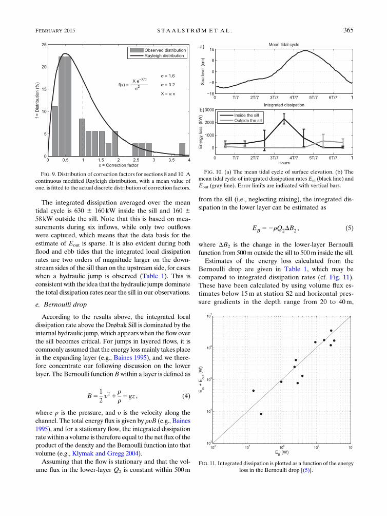
The integrated dissipation averaged over the mean

tidal cycle is 630 6 160 kW inside the sill and 160 658 kW outside the sill. Note that this is based on mea-

surements during six inflows, while only two outflows

were captured, which means that the data basis for the

estimate of Eout is sparse. It is also evident during both

flood and ebb tides that the integrated local dissipation

rates are two orders of magnitude larger on the down-

stream sides of the sill than on the upstream side, for cases

when a hydraulic jump is observed (Table 1). This is

consistentwith the idea that the hydraulic jumps dominate

the total dissipation rates near the sill in our observations.

e. Bernoulli drop

According to the results above, the integrated local

dissipation rate above theDrøbak Sill is dominated by theinternal hydraulic jump, which appears when the flow overthe sill becomes critical. For jumps in layered flows, it iscommonly assumed that the energy lossmainly takes placein the expanding layer (e.g., Baines 1995), and we there-

fore concentrate our following discussion on the lower

layer. The Bernoulli functionBwithin a layer is defined as

B51

2y2 1

p

r1 gz , (4)

where p is the pressure, and y is the velocity along the

channel. The total energy flux is given by ryB (e.g., Baines

1995), and for a stationary flow, the integrated dissipation

ratewithin a volume is therefore equal to the net fluxof the

product of the density and the Bernoulli function into that

volume (e.g., Klymak and Gregg 2004).

Assuming that the flow is stationary and that the vol-

ume flux in the lower-layer Q2 is constant within 500m

from the sill (i.e., neglecting mixing), the integrated dis-

sipation in the lower layer can be estimated as

EB 52rQ2DB2 , (5)

where DB2 is the change in the lower-layer Bernoulli

function from 500m outside the sill to 500m inside the sill.

Estimates of the energy loss calculated from the

Bernoulli drop are given in Table 1, which may be

compared to integrated dissipation rates (cf. Fig. 11).

These have been calculated by using volume flux es-

timates below 15m at station S2 and horizontal pres-

sure gradients in the depth range from 20 to 40m,

FIG. 9. Distribution of correction factors for sections 8 and 10. A

continuous modified Rayleigh distribution, with a mean value of

one, is fitted to the actual discrete distribution of correction factors.

FIG. 10. (a) The mean tidal cycle of surface elevation. (b) The

mean tidal cycle of integrated dissipation rates Ein (black line) and

Eout (gray line). Error limits are indicated with vertical bars.

FIG. 11. Integrated dissipation is plotted as a function of the energy

loss in the Bernoulli drop [(5)].

FEBRUARY 2015 S TAAL STRØM ET AL . 365

calculated from density profiles 500m inside and outside

the sill. In these calculations we assume that the energy

loss in the upper layer is negligible, the velocity head

difference is small compared to the pressure difference,

and the lower-layer volume flux at S2 is equal to the

bottom-layer flux over the sill. For further discussion of

the method see Klymak and Gregg (2004).

The values of the estimates from the measurements

and the Bernoulli drops are surprisingly similar (corre-

lation coefficient of 0.87), given the large number of

assumptions and uncertainties in the estimates, and this

provides a certain amount of credibility both to the es-

timates and the assumptions. This also means that the

local energy budget is relatively well closed, and there

are no large energy sources or sinks that are not

accounted for in the observations.

f. Relation between bottom sill velocity anddissipation rates

During situations where the lower layer is accelerated,

especially when enhanced by mean baroclinic flow, this

leads to hydraulic jumps that dominate the integrated

dissipation rate above the sill. Thus, it is not surprising

that we find a strong correlation between Ein and the

current measured below sill depth at station S2. The

correlation coefficient between Ein and the current

measured at 22.5m from station S2 in the third power is

0.99. Earlier it is shown that these measurements can be

related to the flow in the lower layer over the sill. This

empirical result can be expressed as

Eemp5Cy32 , (6)

where theproportionality factorC is 5.76 1.73 106kgm21.

Klymak et al. (2010) derived an expression for the in-

tegrated dissipation in the case of linear stratification,

where it is argued that it scales with the barotropic flow

over the sill in the third power. In the limit of two-layer

stratification, we find that the integrated dissipation is

proportional to the flow in the lower layer to the third

power. The result from (6) is plotted together with the

observed Ein in Fig. 3d, and the estimate from (6) is well

within the error range of the observed values.We note that

according to (6) the integrated dissipation reach well above

2000kWduring the unobserved strong inflow after transect

7, but is close to zero in the strong inflow after transect 14.

4. Discussion

a. Influence of mean baroclinic flow on the presenceand strength of hydraulic jumps

As shown in section 3b, internal hydraulic jumps are

present in some but not all flood and ebb tides, and this

cannot be explained by differences in barotropic forcing

alone. In the previous section, we found a strong cor-

relation between the total dissipation rates near the sill

and the energy loss in the lower layer estimated from the

drop in the lower-layer Bernoulli function. In these

calculations, the energy loss in the upper layer was as-

sumed to be zero, and the change in the Bernoulli

function was mainly caused by the interface being lower

downstream than upstream.

The observations at Knight Inlet (Klymak and Gregg

2004) showed that the difference in upstream and

downstream interface, also causing a Bernoulli drop in

their case, was created by the blocking of the lower layer

at the sill, resulting in accumulation upstream and di-

vergence downstream. Blocking, and the associated

asymmetric flow over the sill, is only possible if the flow

is critical (G25 1) at the sill. Thus, a hydraulic jump and

the associated energy loss and interface drop are only

possible if the flow is strong enough to obtain critical

flow at the sill.

The observed tidal-averaged baroclinic exchanges

(Fig. 3b; section 3a) probably explain why hydraulic

jumps and large energy losses are absent on one side of

the sill and enhanced on the other during some tidal cy-

cles. During the first four tidal cycles there is a mean in-

ward flow in the bottom that increases the value of G2

during flood and decreases it during ebb tides. Therefore,

the flow is controlled during a larger fraction of the flood

tide. The mean baroclinic two-layer flow must be caused

by a mean difference in interface height over the sill.

During flood tide the change in interface height caused

by the tidal flow adds to the mean interface height

difference, which increases the energy loss. During ebb

tide the value of G2 decreases because of the mean

inflow in the lower layer; the interface difference

caused by the tidal flow is opposite that of the mean

flow, and the flow therefore never reaches critical flow

at the sill. At the end of the observational period, the

mean bottom-layer flow is outward, decreasing the

value of G2 during flood and increasing it during ebb

tides. A reasonable explanation for the missing hy-

draulic jumps therefore is that the mean baroclinic

exchange pushes the flow below the limit of a con-

trolled situation during those occasions where hy-

draulic jumps are not present.

To support this conclusion, we investigate, using two-

layer theory, the magnitude of the barotropic current at

which the flow becomes critical at the sill for a given

baroclinic current. The equations to solve are

G25 1, (7)

where G is given by (2),

366 JOURNAL OF PHYS ICAL OCEANOGRAPHY VOLUME 45

y15q02 q

h1and (8)

y2 5q01 q

h2, (9)

where q0 and q are the barotropic and baroclinic volume

fluxes in deep water, and the Bernoulli equation

1

2(y222 y21)2 g*h15 constant , (10)

where we have used the rigid-lid approximation for the

surface boundary condition. Thequantity g* [5g(r22 r1)/

r1] is the reduced gravity. Note that the barotropic volume

fluxes in deep water are not barotropic over the sill.

The solution can be written in terms of the non-

dimensional variables Fr5 q0/(H2 d)/c1, Frbc5 q/(H2d)/c1, h10/(H 2 d), and d/H:

f (Fr, Frbc,h10/(H2 d), d/H)5 0, (11)

where Frbc is the baroclinic Froude number, h10 is the

deep-water upper-layer depth,H is the total water depth

away from the sill, and d is the sill height. The solution

curves are shown in Fig. 12 for selected values of h10/

(H2 d), and d/H5 0.8. These curves may be seen as the

outer limits for subcritical flow over the sill, since (7) is

fulfilled along these lines. The dashed lines show when the

upstream flow becomes critical. Examples relevant for the

Oslofjord are indicated with black circles connected with

lines, corresponding to a barotropic Froude number os-

cillating between 60.45. The relevant solution curves in

this case are those forh10/(H2d)5 0.5. For zero baroclinic

mean flow, the flow at the sill becomes critical for jFrj .0.36. For Frbc 5 0.3, corresponding approximately to the

situation at the beginning of the observational period in

2011with inwardmean flow in the bottom layer, the flow is

critical for Fr . 20.05 and subcritical for 20.62 , Fr ,20.05. This corresponds well with the observed absence of

a hydraulic jump during ebb tide in the Oslofjord during

this period. According to this theory, hydraulic jumps start

to appear during ebb tides, when the baroclinic Froude

number drops below 0.11. Our observations are not de-

tailed enough to confirm this prediction, but the theory

supports the hypothesis that the observed baroclinic mean

flows can push the conditions beyond the limit when hy-

draulic jumps do not occur during the tidal phases when

they are opposed by the bottom-layer baroclinic flow.

b. Energy partition

So far we have mainly discussed the dissipation rates

near the sill. We know that there is also an energy flux

away from the sill mediated by propagating internal

waves (Staalstrøm et al. 2012). Thus, the question we

pose is how the barotropic energy loss is partitioned

between local energy loss and radiated energy that may

cause mixing further into the fjord.

Staalstrøm et al. (2012) calculated the energy flux due to

internal waves (FIW) into the fjord at station S2 from

measurements of temperature, salinity, and currents during

August 2009 with several methods. The method we trust

most used a correlation term of baroclinic pressure and

baroclinic velocity described by Kunze et al. (2002), giving

FIW5 1906 90kW. If we combine this estimate with the

presently obtained results Ein 5 630 6 160 kW, we find

that about 60%–90% of the total energy loss inside the

Drøbak Sill dissipates within 500m from the sill.

Our estimate of the barotropic energy dissipation near

the sill is much higher than the 33% in the Canadian

Knight Inlet (Klymak and Gregg 2004) and about the

same as the 60%–80% in the Scottish Loch Etive (Inall

et al. 2004). The Froude numbers equal 0.75 in Knight

Inlet, 1.8 in Loch Etive, and only 0.45 in the Oslofjord.

With these numbers it is surprising that the fraction of

local dissipation in the Oslofjord is as high as in Loch

Etive, which have much stronger currents relative to the

stratification andmuch larger than the fraction at Knight

Inlet, which is known to have powerful hydraulic jumps.

One important factor for internal wave generation is the

vertical level of the pycnocline as compared to the height of

the sill. In LochEtive the upper layer extends all theway to

the sill and therefore the bottom layer is blocked and in-

ternal tides have to be generated irrespectively of the hy-

draulics on the sill, whereas in the Oslofjord the bottom

FIG. 12. Baroclinic Froude number Frbc 5 q/(H 2 d)/c1 vs baro-

tropic Froude number Fr5 q0/(H2 d)/c1 for solutions with critical

conditions at the sill (full lines), and upstream of the sill (dashed),

sill height d/H 5 0.8, and upper-layer depth h10/(H 2 d) 5 0.25

(blue), 0.5 (black), and 0.75 (red). Also shown are trajectories

corresponding tomean baroclinic Froude number of 0, 0.11, and 0.3

and barotropic Froude number cycling between 60.45 (black cir-

cles connected by lines).

FEBRUARY 2015 S TAAL STRØM ET AL . 367

layer is not blocked unless there is critical conditions on the

sill, meaning that first-mode internal waves may not always

be generated (see the discussion in section 4a). This does,

however, not explain why Knight Inlet is a more efficient

wave generator than the Oslofjord.

Another factor that may explain the large fraction of

local dissipation at the Oslofjord sill is that not only the

tides cause the dissipation but also the mean baroclinic

flow. Therefore, the fraction of barotropic tidal energy

that dissipates locally is probably overestimated in this

study. The interaction between the tidal flow and the

mean baroclinic flow is highly nonlinear, and in the

present study we see no way to separate these two en-

ergy sources. This must be left for future studies.

Although detailed studies of the hydraulic jumps in

three fjords (Knight Inlet, LochEtive, and theOslofjord)

have increased our understanding of the internal hy-

draulics and energetics near fjord sills, there are still

many questions to answer regarding the relation be-

tween local energy loss and internal tide radiation and

the influence of stratification, tidal flow strength, and sill

geometry. We are presently looking into these issues

with numerical and theoretical work.

Acknowledgments. This project was funded by

the Norwegian Research Council (Project 184944).

Lars Arneborg was supported by the Swedish Research

Council through Grant 621-2008-2689. The field work

would not have been possible without the assistance of the

crew on board the R/V Trygve Braarud. Thanks are also

due to Eyvind Aas and Lars Petter Røed for constructivediscussions and suggestions.

REFERENCES

Afanasyev, Y. D., and W. R. Peltier, 2001: Reply to comment on

the paper on breaking internal waves over the sill in Knight

Inlet. Proc. Roy. Soc. London, A457, 2831–2834, doi:10.1098/

rspa.2001.0801.

Armi, L., 1986: The hydraulics of two flowing layers with different den-

sities. J. Fluid Mech., 163, 27–58, doi:10.1017/S0022112086002197.Arneborg, L., 2004: Turnover times for the water above sill level in

Gullmar Fjord. Cont. Shelf Res., 24, 443–460, doi:10.1016/

j.csr.2003.12.005.

——, and B. Liljebladh, 2009: Overturning and dissipation caused

by baroclinic tidal flow near the sill of a fjord basin. J. Phys.

Oceanogr., 39, 2156–2174, doi:10.1175/2009JPO4037.1.

Aure, J., J. Molvær, and A. Stigebrandt, 1996: Observations of inshore

water exchange forcedby afluctuating offshore density field.Mar.

Pollut. Bull., 33, 112–119, doi:10.1016/S0025-326X(97)00005-2.

Baines, P. G., 1995: Topographic Effects in Stratified Flows. Cam-

bridge University Press, 482 pp.

Cummins, P. F., 2000: Stratifiedflowover topography:Time-dependent

comparisons between model solutions and observations. Dyn.

Atmos. Oceans, 33, 43–72, doi:10.1016/S0377-0265(00)00044-0.Farmer, D. M., and R. A. Denton, 1985: Hydraulic control of flow

over the sill in Observatory Inlet. J. Geophys. Res., 90, 9051–

9068, doi:10.1029/JC090iC05p09051.

——, and L. Armi, 1999: Stratified flow over topography: The role

of small-scale entrainment and mixing in flow establishment.

Proc. Roy. Soc. London, A455, 3221–3258, doi:10.1098/

rspa.1999.0448.

Inall, M., F. Cottier, C. Griffiths, and T. Rippeth, 2004: Sill dy-

namics and energy transformation in a jet fjord. Ocean Dyn.,

54, 307–314, doi:10.1007/s10236-003-0059-2.

——, T. Rippeth, C. Griffiths, and P. Wiles, 2005: Evolution and

distribution of TKE production and dissipation within strati-

fied flow over topography. Geophys. Res. Lett., 32, L08607,

doi:10.1029/2004GL022289.

Klymak, J.M., andM.C.Gregg, 2001: Three-dimensional nature of

flow near a sill. J. Geophys. Res., 106, 22 295–22 311,

doi:10.1029/2001JC000933.

——, and ——, 2003: The role of upstream waves and a down-

stream density pool in the growth of lee waves: Stratified flow

over the Knight Inlet sill. J. Phys. Oceanogr., 33, 1446–1461,

doi:10.1175/1520-0485(2003)033,1446:TROUWA.2.0.CO;2.

——, and——, 2004: Tidally generated turbulence over the Knight

Inlet sill. J. Phys. Oceanogr., 34, 1135–1151, doi:10.1175/

1520-0485(2004)034,1135:TGTOTK.2.0.CO;2.

——, S. Legg, and R. Pinkel, 2010: A simple parameterization of

turbulent tidal mixing near supercritical topography. J. Phys.

Oceanogr., 40, 2059–2074, doi:10.1175/2010JPO4396.1.

Kunze, E., L. K. Rosenfeld, G. S. Carter, and M. C. Gregg, 2002:

Internal waves in the Monterey Submarine Canyon. J. Phys.

Oceanogr., 32, 1890–1913, doi:10.1175/1520-0485(2002)032,1890:

IWIMSC.2.0.CO;2.

Ledwell, J. R., E. T. Montgomery, K. L. Polzin, L. C. S. Laurent,

R. W. Schmitt, and J. M. Toole, 2000: Evidence for enhanced

mixing over rough topography in the abyssal ocean. Nature,

403, 179–182, doi:10.1038/35003164.

Lepland,A., R. Bøe, A. Lepland, andO. Totland, 2009:Monitoring

the volume and lateral spread of disposed sediments by

acoustic methods, Oslo Harbor, Norway. J. Environ. Manage.,

90, 3589–3598, doi:10.1016/j.jenvman.2009.06.013.

Nash, J. D., and J. N. Moum, 2001: Internal hydraulic flows on the

continental shelf: High drag states over a small bank. J. Geo-

phys. Res., 106, 4593–4611, doi:10.1029/1999JC000183.

Prandke, H., and A. Stips, 1998: Test measurements with an opera-

tional microstructure-turbulence profiler: Detection limit of dis-

sipation rates.Aquat. Sci., 60, 191–209, doi:10.1007/s000270050036.

Staalstrøm, A., E. Aas, and B. Liljebladh, 2012: Propagation and

dissipation of internal tides in the Oslofjord. Ocean Sci., 8,

525–543, doi:10.5194/os-8-525-2012.

Stacey,M.W., 1984: The interaction of tides with the sill of a tidally

energetic inlet. J. Phys. Oceanogr., 14, 1105–1117, doi:10.1175/

1520-0485(1984)014,1105:TIOTWT.2.0.CO;2.

Stashchuk, N., M. Inall, and V. Vlasenko, 2007: Analysis of su-

percritical tidal flow in a Scottish fjord. J. Phys. Oceanogr., 37,

1793–1810, doi:10.1175/JPO3087.1.

Stigebrandt, A., 1976: Vertical diffusion driven by internal waves in

a sill fjord. J. Phys. Oceanogr., 6, 486–495, doi:10.1175/

1520-0485(1976)006,0486:VDDBIW.2.0.CO;2.

——, 1999: Resistance to barotropic tidal flow in straits by baro-

clinic wave drag. J. Phys. Oceanogr., 29, 191–197, doi:10.1175/

1520-0485(1999)029,0191:RTBTFI.2.0.CO;2.

——, and J.Aure, 1989: Verticalmixing in basinwaters of fjords. J. Phys.

Oceanogr., 19, 917–926, doi:10.1175/1520-0485(1989)019,0917:

VMIBWO.2.0.CO;2.

Tryggestad, S., 1974: A survey of current conditions at Brenntangen

and tides in the Oslofjord (in Norwegian). University of Oslo

Tech. Rep., 120 pp.

368 JOURNAL OF PHYS ICAL OCEANOGRAPHY VOLUME 45