Evaluation of Turbulence Model Corrections for SupersonicJets using the OVERFLOW Code

Nico Gross,∗ Gregory A. Blaisdell,† and Anastasios S. Lyrintzis‡

Purdue University, West Lafayette, IN 47907

The OVERFLOW code is used for computations of supersonic jets. Corrections for compressibility andtemperature effects are evaluated based on comparisons with experimental data. Test cases include isother-mal and heated, perfectly expanded and underexpanded axisymmetric jets with design Mach numbers aroundtwo. Also, a 3-D jet in an angled crossflow at a design Mach number of three is evaluated. The SST turbulencemodel is chosen for the flows examined in this study. The Sarkar, Zeman, and Wilcox compressibility correc-tions and Abdol-Hamid’s temperature correction are assessed when used with the SST model. Results for theaxisymmetric jets show that using a compressibility correction is important for a good prediction of the jetdevelopment. The effect of the temperature correction is not as significant. For the 3-D jet in crossflow, con-clusions are not as decisive. The velocity decay is underpredicted when using the compressibility correction.The temperature correction behaves as it did for the axisymmetric jet. The overall recommendation is thatthe corrections must be used with caution, especially when approaching high temperature and Mach numberregimes.

Nomenclature

a = speed of soundCC = compressibility correctionCµ = eddy viscosity coefficientD = nozzle exit diameterεd = dilatation dissipationεs = solenoidal dissipationk = kinetic energy of turbulence fluctuationsM = Mach numberMt = turbulence Mach numberPR = pressure ratioR = radial (crossflow) coordinateR1/2 = jet half radiusT = jet temperatureTC = temperature correctionTR = temperature ratioTinf = ambient temperatureTg = temperature gradientU = jet velocity in X-directionUjet = jet centerline velocity in X-direction at nozzle exit planeVel = jet velocity magnitudeX = axial (streamwise) coordinateγ = specific-heat ratioω = specific dissipation rate

∗Graduate Research Assistant, School of Aeronautics and Astronautics, Student Member AIAA.†Associate Professor, School of Aeronautics and Astronautics, Associate Fellow AIAA.‡Professor, School of Aeronautics and Astronautics, Associate Fellow AIAA.

1 of 21

American Institute of Aeronautics and Astronautics

I. Introduction

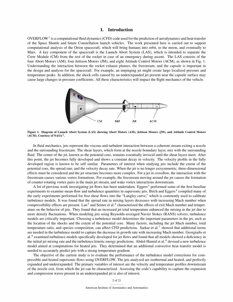
OVERFLOW1 is a computational fluid dynamics (CFD) code used for the prediction of aerodynamics and heat transferof the Space Shuttle and future Constellation launch vehicles. The work presented here is carried out to supportcomputational analysis of the Orion spacecraft, which will bring humans into orbit, to the moon, and eventually toMars. A key component of the spacecraft is the Launch Abort System (LAS), which is intended to separate theCrew Module (CM) from the rest of the rocket in case of an emergency during ascent. The LAS consists of thefour Abort Motors (AM), four Jettison Motors (JM), and eight Attitude Control Motors (ACM), as shown in Fig. 1.Understanding the interaction between the rocket exhaust plumes, the freestream, and the capsule is important inthe design and analysis for the spacecraft. For example, an impinging jet might create large localized pressure andtemperature peaks. In addition, the shock cells caused by an underexpanded jet present near the capsule surface maycause large changes in pressure coefficients. All these characteristics will impact the flight mechanics of the vehicle.

Figure 1. Diagram of Launch Abort System (LAS) showing Abort Motors (AM), Jettison Motors (JM), and Attitude Control Motors(ACM). Courtesy of NASA 2.

In fluid mechanics, jets represent the viscous and turbulent interaction between a coherent stream exiting a nozzleand the surrounding freestream. The shear layers, which form at the nozzle boundary layer, mix with the surroundingfluid. The center of the jet, known as the potential core, remains essentially inviscid until the shear layers meet. Afterthis point, the jet becomes fully developed and shows a constant decay in velocity. The velocity profile in the fullydeveloped region is known to be self similar. Parameters of interest when studying jets include the extent of thepotential core, the spread rate, and the velocity decay rate. When the jet is no longer axisymmetric, three-dimensionaleffects must be considered and the jet structure becomes more complex. For a jet in crossflow, the interaction with thefreestream causes various vortex formations. For example, the freestream moving around the jet causes the formationof counter-rotating vortex pairs in the main jet stream, and wake vortex interactions downstream.

A lot of previous work investigating jet flows has been undertaken. Eggers3 performed some of the first baselineexperiments to examine mean-flow and turbulence quantities in supersonic jets. Birch and Eggers4 compiled many ofthe early experiments performed for free shear flows into the “Langley curve,” which is commonly used to calibrateturbulence models. It was found that the spread rate in mixing layers decreases with increasing Mach number whencompressibility effects are present. Lau5 and Seiner et al.6 characterized the effects of exit Mach number and temper-ature on the behavior of jets. They found that an increased jet total temperature enhanced the mixing in the jet due tomore density fluctuations. When modeling jets using Reynolds-averaged Navier Stokes (RANS) solvers, turbulencemodels are critically important. Choosing a turbulence model determines the important parameters in the jet, such asthe location of the shocks and the extent of the potential core. Many factors, including the jet Mach number, totaltemperature ratio, and species composition, can affect CFD predictions. Sarkar et al.7 showed that additional termsare needed in the turbulence model to capture the decrease in growth rate with increasing Mach number. Georgiadis etal.8 examined turbulence models specifically developed for jet flows and found that all models showed a deficiency inthe initial jet mixing rate and the turbulence kinetic energy predictions. Abdol-Hamid et al.9 devised a new turbulencemodel aimed at computations for heated jets. They determined that an additional convective heat transfer model isneeded to accurately predict jets with a strong temperature gradient.

The objective of the current study is to evaluate the performance of the turbulence model corrections for com-pressible and heated supersonic flows using OVERFLOW. The jets analyzed are isothermal and heated, and perfectlyexpanded and underexpanded. The primary variables of interest are the velocity and temperature profiles downstreamof the nozzle exit, from which the jet can be characterized. Assessing the code’s capability to capture the expansionand compression waves present in an underexpanded jet is also of interest.

2 of 21

American Institute of Aeronautics and Astronautics

II. Test Cases

In order to assess OVERFLOW’s ability to model supersonic jets, several test cases are computed. Various ax-isymmetric jet experiments are selected. Then, a 3-D jet in angled crossflow is used to assess further parameters ofinterest which could not be studied using axisymmetric jets. Experimental data measured using particle image ve-locimetry (PIV) and pressure probes in the flow field is available for comparison to CFD results. The experiments arechosen based on the quality of the data and the parameters of interest. Key conditions for the test cases considered aresummarized in Table 1.

Table 1. Reference conditions for test cases considered

Test Case Classification Mnozzle P0/P0,∞ T0/T0,∞Eggers isothermal, perfectly expanded 2.2 11.0 1.0Wishart heated, perfectly expanded 2.0 7.6 2.3Wishart heated, underexpanded 2.0 9.5 2.3Glenn heated, underexpanded 3.0 28.5 2.3

A. Eggers Jet

The Eggers3 jet refers to a 1966 experiment characterizing supersonic turbulent jets. A Mach 2.22 isothermaljet with nozzle exit diameter of 1.01” (0.026 m) was exhausted into ambient air, with a pressure ratio of 11. Theexperiment supplies velocity profiles in the near- and far-field of the jet. This experiment provides a standard test casefor supersonic jet validation.

B. Wishart Jet

The Wishart10 experiment, performed at Florida State University, is a similar study to that of Eggers, but withconditions more closely resembling those of the LAS. The jet used a nozzle designed for Mach 2, a nozzle exitdiameter of 1.15” (0.029 m), and was operated at ideal and off-design conditions. All cases were run isothermal andheated. These conditions allow for examination of the shock-cell structure and temperature effects on the developmentof the jet. The cases of interest for this study are the heated jet (temperature ratio 2.3) for perfectly expanded (pressureratio 7.65) and underexpanded (pressure ratio 9.3) conditions. The complete set of computational analysis performedfor this experiment can be found in the author’s Master’s thesis11.

C. Glenn Jet

The Glenn jet experiment (Wernet et al.12), performed at the NASA Glenn Research Center, was used to acquiredata for a hot supersonic jet in subsonic crossflow. It was performed as part of the aerodynamics analysis and designprocess for the LAS. While actual LAS flight conditions were not attainable, the jet conditions used here were atthe highest possible pressures and temperatures attainable in the test facility, which were stagnation pressure andtemperature of 410 psi (2.8×106 Pa) and 1350 R (750 K), respectively. A survey of available literature showed thatno other experiments had been performed at similar conditions. The nozzle was placed in a wind tunnel with coldfreestream air at Mach 0.3. The jet air was heated using a natural gas combustor and exhausted through the conicalnozzle at an angle of 25 degrees relative to the freestream. The nozzle exit design Mach number was 3.0, but due tothe underexpansion, Mach numbers exceeding four are seen downstream. Experimental data were obtained with PIVat various locations downstream of the nozzle exit and normal to the freestream, producing two dimensional velocityvector fields.

III. Numerical Methods

A. Code Description

The OVERFLOW code1 is an overset grid solver developed by NASA. It solves the time-dependent, Reynolds-averaged Navier-Stokes equations for compressible flows. The overset capability makes it useful for computing flow

3 of 21

American Institute of Aeronautics and Astronautics

fields involving complex geometries. The code is formulated using a finite difference method and has various centraland upwind schemes for spatial discretization built in. A diagonalized, implicit approximate factorization (ADI)scheme is used for time advancement. Other capabilities, such as local time-stepping and grid sequencing, are alsoavailable to accelerate convergence.

B. Turbulence Models and Corrections

Choosing the correct turbulence model is critical for a good computational prediction of the flowfield. The OVER-FLOW code contains various algebraic, one-equation, and two-equation turbulence models. This study will examinefour of the most popular models: the Spalart-Allmaras (SA) model13, Baldwin-Barth (BB) model14, k-ω model15

(1988 version), and Shear Stress Transport (SST) model16. All turbulence models use the Boussinesq approximationto incorporate the contribution of the Reynolds stresses through an eddy viscosity into the Navier-Stokes equations.The SA and BB models are one-equation models which solve for the eddy viscosity, while the k-ω and SST solve twopartial differential equations for the turbulence kinetic energy, k, and the specific dissipation rate, ω. The SST modelis a hybrid between the k-ε and k-ω models, where a function is used to blend between the models based on distanceto the nearest wall.

Current turbulence models have been designed for low-speed, isothermal flows. Future research should strive todevelop a new model that is general for all types of flows. However, at this time, the practical approach is to modifyexisting models for more complicated flows. The intent of this study is to assess the various corrections for turbulencemodels that are applicable to the LAS jet flows, namely compressibility and high temperature corrections.

The compressibility correction is devised to deal with additional effects seen for higher Mach number flows,specifically, the effects of compressibility on the dissipation rate of the turbulence kinetic energy. For free shearflows, this is exhibited as the decrease in growth rate in the mixing layer with increasing Mach number4. Standardturbulence models do not account for this Mach number dependence, and thus a compressibility correction is used. Forcompressible flows, two extra terms, known as the dilatation dissipation, εd, and the pressure-dilatation occur in theturbulence kinetic energy equation. The pressure-dilatation term is usually neglected because its contributions havebeen shown to be small15. The dilatation dissipation term is included in addition to the solenoidal, or incompressible,dissipation, εs. In the formulation of the k-ω and SST models, the extra term also occurs in the specific dissipationrate equation. Thus, the effect is that the growth rate of turbulence is inhibited when the correction is active. Sarkar7

modeled the ratio of the dilatation dissipation to the solenoidal dissipation, εd/εs, as a function of the turbulence Machnumber, Mt, defined as

Mt =

√2k

a(1)

For Sarkar’s model,

εd

εs= F (Mt) = M2

t (2)

The model proposed by Zeman17 is formulated as follows

F (Mt) ={

1− exp

[−1

2(γ + 1)(Mt −Mt0)2/Λ2

]}H(Mt −Mt0) (3)

where Mt0 = 0.10√

2/(γ + 1) and H(x) is the Heaviside function. Finally, Wilcox’s15 model is given by

F (Mt) = (M2t −M2

t0)H(Mt −Mt0) (4)

The model constant Mt0 = 0.25. For a complete discussion of the compressibility corrections, see Wilcox15. Itmust also me noted that the implementation of the SST turbulence model in OVERFLOW follows that by Suzen andHoffman18, where the compressibility correction is multiplied by the SST blending function, thus effectively disablingthe correction in near wall regions.

Abdol-Hamid et al.9 noticed that standard turbulence models also fail to capture the increase in the shear layergrowth rate due to temperature effects observed by Lau and Seiner et al. They devised a new correction to deal withthese effects. The model was calibrated to the supersonic jet experiment of Seiner et al.6. The correction calculates amodified eddy viscosity coefficient, Cµ, based on the normalized total temperature gradient, Tg , in the flow,

4 of 21

American Institute of Aeronautics and Astronautics

Cµ = 0.09

[1 +

T 3g

0.041 + f(Mt)

](5)

F (Mt) is the same as in Eq. 4 above, except the model constant Mt0 = 0.1. From this formulation, a large totaltemperature gradient causes an increase in the eddy viscosity, which thus increases the diffusion in the jet. The cor-rection also considers the compressibility effects by including the F (Mt) term. For a large turbulence Mach number,the eddy viscosity coefficient would be decreased and would suppress the mixing. The compressibility effects in thetemperature correction’s F (Mt) term are calculated separately from those of an implicit compressibility correctionsuch as Sarkar’s. However, for Abdol-Hamid’s supersonic jet test case9, all analysis is completed while also usingSarkar’s compressibility correction, and this approach is followed for this work as well.

C. Grid Generation

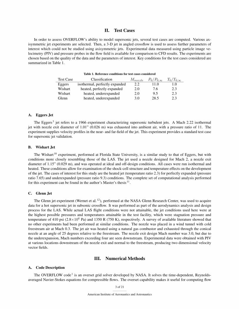
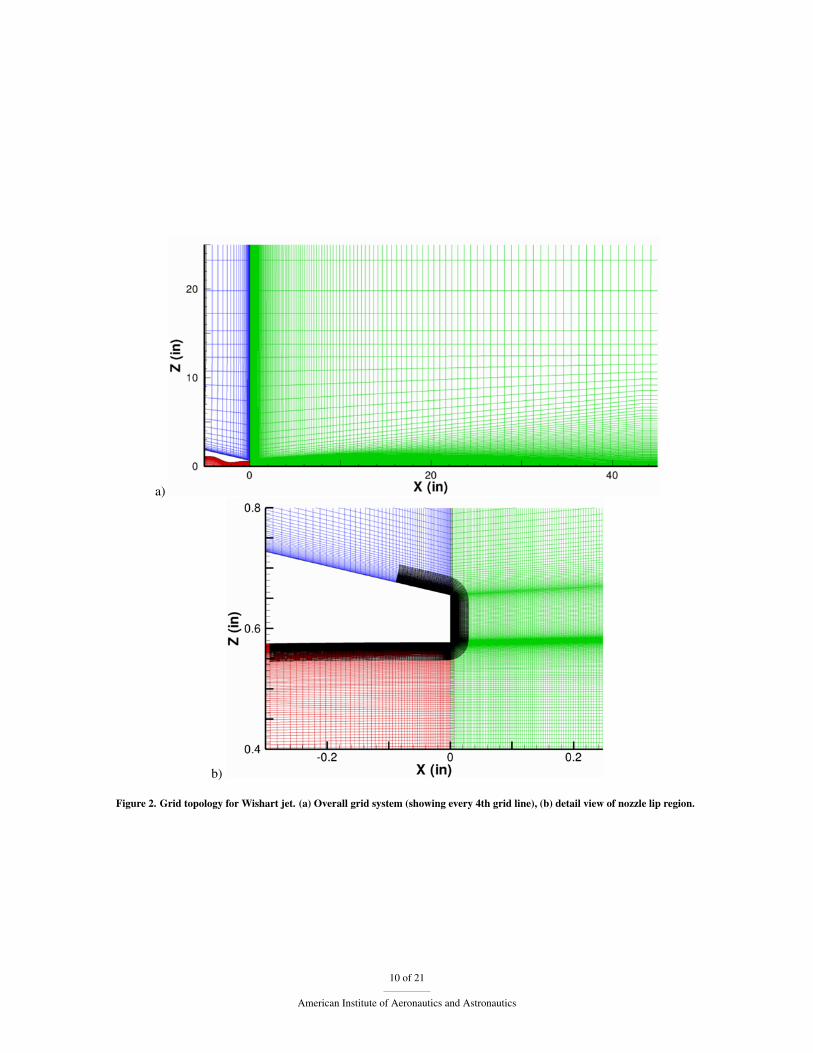
Grids for the Eggers and Wishart jets are very similar. The grid for the axisymmetric jets is shown in Fig. 2. Fourzones are used for the nozzle, top, aft, and the nozzle lip regions. The X-axis represents the jet’s axis of symmetry.The collar grid around the nozzle lip is used to better resolve the high flow gradients present in this region. The gridspacing along the inner nozzle boundary is designed to keep the wall y+ below one in order to adequately resolve theviscous sublayer near the wall. The grid is particularly fine in the aft region off the nozzle lip to resolve the shearlayer that determines the jet development. In order to sufficiently model the freestream and eliminate upper and aftboundary effects, the domain of the plume extends at least 30 diameters in the radial and 80 diameters in the axialdirections, measured from the nozzle exit plane. The final Eggers and Wishart grid systems contained 91.3×103 and105.8×103 grid points, respectively.

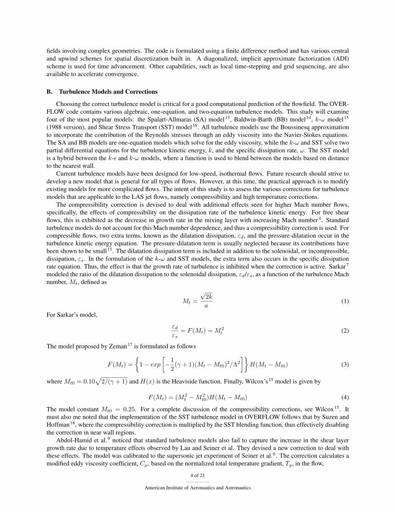
For the Glenn jet, grid scripts were obtained from researchers at NASA Ames Research Center. The model includesthe entire wind tunnel. Similar to the grids for the axisymmetric jets, particular attention is paid to ensure sufficientresolution along the nozzle lip and the mixing region. For the final grid, the plume region contained nine million gridpoints, leading to a total of 29×106 grid points. Figure 3 shows the grid for the Glenn jet along the centerline plane.

D. Boundary Conditions

For the axisymmetric jet, freestream boundary conditions are imposed at the top of the nozzle, with Mach 0.01 andstandard pressure and temperature. For the Glenn jet, the freestream boundary conditions are imposed at the tunnelentrance with Mach 0.3. All walls are specified as viscous and adiabatic. The nozzle conditions are set as a ratioof stagnation pressure and temperature from the nozzle plenum to the freestream. For the Glenn jet, the natural gascombustion products in the nozzle are modeled as a second species with specific heats ratio, γ, of 1.32. The top andaft domain boundaries are specified as pressure outflow boundaries with a given value of static pressure.

E. Solution Method

The numerical schemes used are chosen based on robustness and rate of convergence. For consistency, all test casesuse the same inputs for the numerical methods. The HLLC upwind scheme proved better than the central differenceand Roe’s upwind scheme for the discretization of the spatial derivatives. This is especially true for cases in whichshocks are present, as the HLLC is an improved algorithm for capturing shocks with low smearing. A van Albadalimiter is used for the upwind Euler terms, along with a MUSCLE scheme flux limiter for added smoothing. Thespatial differencing for all convective terms uses third order accuracy. Local timestep scaling with a constant CFLnumber is employed, where the timestep scaling is based on the local cell Reynolds number. All cases are run withthree levels of grid sequencing for improved convergence. 1,000 iterations are run on the coarse and medium gridlevels each before running 6,000 iterations on the fine grid. The solution is considered converged when all residualsdrop at least three orders of magnitude and momentum forces at various downstream locations are constant.

All calculations for the axisymmetric jet are run on a 128 processor cluster at NASA JSC consisting of 64 1.3GHz and 64 1.5 GHz processors and 124 GB RAM. Runs are split between 20 processors and use an average of 10CPU hours for the final grid. For the 3-D jet, cases are run on the NASA Advanced Supercomputing (NAS) clusterColumbia using 64 CPUs, with an average CPU time between 1500 and 1800 hours, depending on the case. A small(13%) increase in computation time is observed when using the temperature correction.

5 of 21

American Institute of Aeronautics and Astronautics

F. Grid Convergence

Free shear flows such as this jet flow are sensitive to the computational grid. A grid that is too coarse may show anoverly diffusive behavior. Grid refinement is thus performed to ensure that the solution is grid independent. Resultsare shown only for the underexpanded jet as this case showed the most sensitivity to the grid. The grid is refinedin the regions of interest: the end of the nozzle and plume where mixing with the freestream occurs. The numberof grid points in each direction is doubled successively. The centerline velocity profiles downstream are sensitiveto grid refinement and important to the analysis. Figure 4 shows the centerline Mach number for three levels ofgrid refinement, with 12.1×103, 48.5×103, and 196.0×103 grid points in the plume region. The most significantdistinction is seen in the resolution of the shock cells. While all grids predict the length of the shock cells equally, thepeak is smeared with the coarsest grid, where the peak Mach number is only 2.58, compared with 2.72 and 2.87 for themedium and fine grids, respectively. After the potential core, there is very little difference in the results. It is decidedthat the medium resolved all parameters of interest sufficiently, and thus is used in all subsequent computations. Asimilar study (not presented here) showed that the grid for the 3-D jet is also grid independent.

IV. Results

A. Eggers Jet

The goal of the Eggers jet runs is to evaluate the baseline turbulence model performance. Figure 5a shows the jetcenterline velocity, normalized by the jet exit velocity, as a function of downstream distance, normalized by jet exitdiameter, for various uncorrected turbulence models. The velocity remains constant through the jet potential core,and then decays in the fully developed region. The SST, k-ω, and SA models predict too much turbulent mixing,thus showing a potential core length that is shorter than that of the experiment. The BB model, on the other hand,significantly underpredicts the mixing and exhibits an excessively long potential core. The SST model gives the bestprediction, especially further downstream.

Figure 5b shows the jet half radius for the turbulence models. The half radius is defined as the radius at which thevelocity is 50% of the local centerline velocity, computed at all downstream (X) locations. This gives a representationof the jet’s spreading rate. It can be seen that because of the increased mixing by the SST, k-ω, and SA models, thespread rate is also overpredicted. The BB model does not show enough mixing and does not spread as quickly. TheSST model matches the experimental spread rate most closely. Based on this preliminary analysis, the SST turbulencemodel is chosen for all subsequent computations.

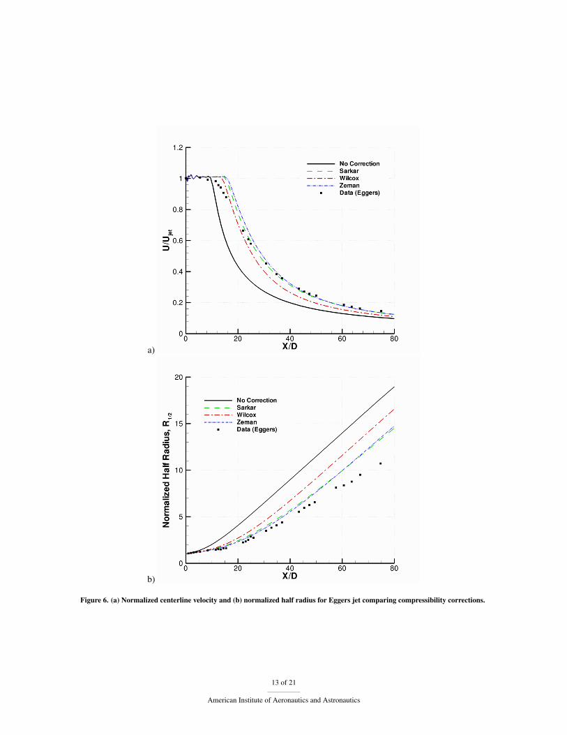
Figure 6 compares the compressibility corrections by Sarkar, Zeman, and Wilcox, which were implemented intothe SST model in the OVERFLOW source code. All three show a noteworthy improvement over not using anycorrection. Wilcox’s model diffuses slightly more quickly compared with the experimental data. There is no significantdifference between the Sarkar and Zeman models. In Fig. 6b, the spread rate for the three compressibility correctionsis presented. Analogous to the centerline velocity, the Sarkar and Zeman corrections show the best performance, andall corrections show a significant improvement over the uncorrected model. There is no major difference between thethree compressibility corrections examined, and hence Sarkar’s model will be used for all further analysis.

B. Heated Wishart Jet

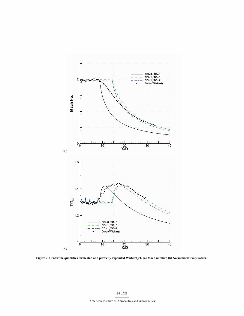
Figure 7a presents the centerline Mach number for the heated Wishart jet. The plot shown contains the baselineturbulence model (CC=0, TC=0), the model with Sarkar’s compressibility correction (CC=1, TC=0), and the modelwith Abdol-Hamid’s temperature correction and Sarkar’s compressibility correction (CC=1, TC=1). As observedwith the Eggers jet, the compressibility correction decreases turbulent mixing and shifts the curve to the right. Thetemperature correction increases mixing when used with the compressibility correction. It is important to note thatthe compressibility correction has the more pronounced effect on the solution. While the use of no corrections mostclosely matches the experimental potential core length, the downstream behavior is best predicted when using thecompressibility correction.

In Fig. 7b, the temperature profile, normalized by the ambient temperature, is plotted along the centerline. Theincrease in temperature is caused by the compression as the gas decelerates in the shear layer, and then decreases tothe ambient value through mixing with the freestream. All models show an identical magnitude in the temperaturerise, which matches well with the experimental data. Similarly to before, the start of the shear layer is better predicted

6 of 21

American Institute of Aeronautics and Astronautics

without correction, whereas the downstream behavior agrees more closely with the compressibility correction. In bothplots, it is indiscernible whether adding the temperature correction provides a better prediction.

Figure 8 shows radial Mach number profiles for four downstream locations. The difference in jet developmentprediction is clearly demonstrated here. There is no noteworthy distinction between the models for X/D of 3.5 and 7as the jet has not had ample time to mix with the ambient fluid. The compressibility correction again is seen to inhibitmixing, thus showing a longer potential core. For R/D larger than 0.8, all models show a similar prediction as thejet has dissipated into the ambient fluid. For the two later X/D locations, the experimental data lie between the CFDresults, and there is no clear model that exhibits a better behavior. However, at increasing radial distance, the modelwith the compressibility corrections seems to show better agreement with the experimental data.

C. Heated and Underexpanded Wishart Jet

The contour plots of Mach number in Fig. 9 illustrate the behavior of the underexpanded and heated jet. The jet exitpressure is higher than the back pressure and expansion fans are formed at the lip of the jet. Once the expansion wavesreach the jet boundary, they reflect as compression waves to match the constant pressure condition at the boundary.When the pressure ratio is large enough, the compression waves no longer meet at the axis but instead form a strongernormal shock known as the Mach disc. The convergence of the expansion fan generates a cylindrical shock, knownas the barrel shock, which terminates at the Mach disc. This leads to a pattern of shock cells, frequently seen in theexhaust of a jet or rocket engine. The wavelength of the expansion and compressions depends on the Mach numberand pressure ratio. For this case, the maximum Mach numbers are approaching three, much higher than the nozzledesign Mach number of two.

It is evident that the choice of turbulence model correction significantly impacts the development of the shockcells. Using exclusively the compressibility correction (b) shows seven distinguishable shock cells, compared withonly four for the uncorrected model (a). The use of the temperature correction does not change the number of shockcells present, but does slightly decrease the length when used with the compressibility correction (c).

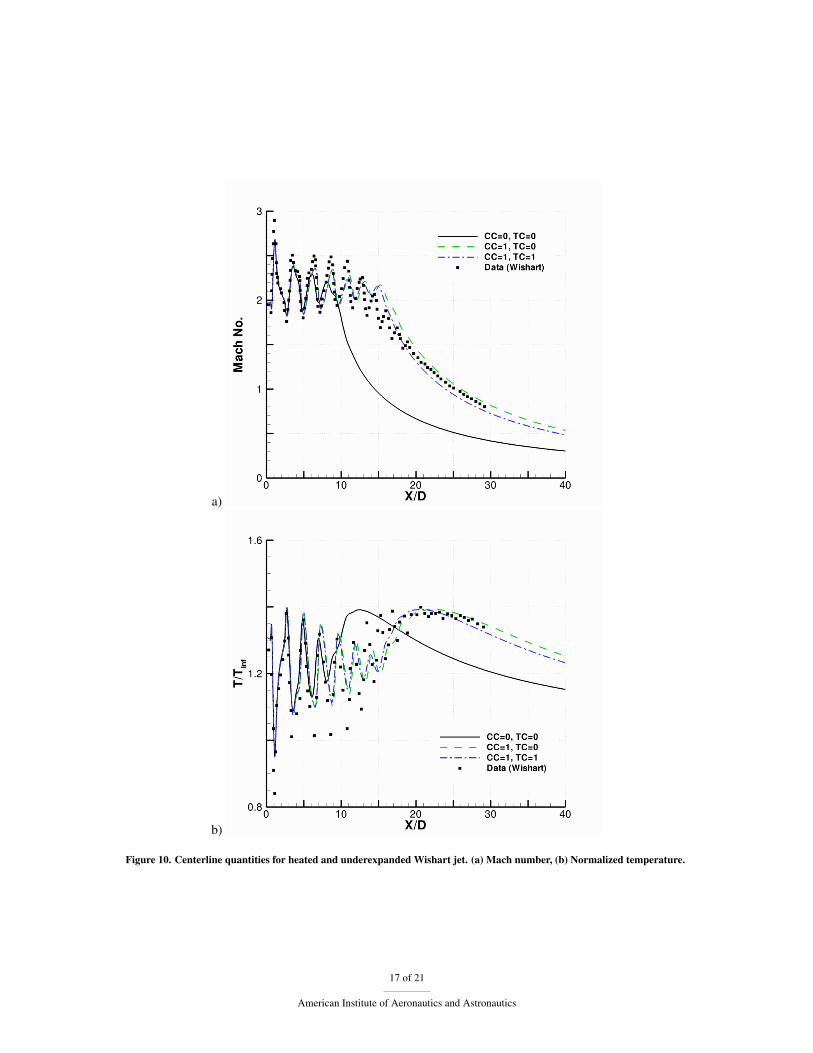
Figures 10a and b show the centerline Mach number and temperature profiles, respectively, for the heated andunderexpanded jet. It is noted that the sharp increases in Mach number (due to expansion fans) correspond to sharpdecreases in temperature, as expected, and the opposite is true for the compressions. The difference in the number ofshock cells present is also visible between the corrections. For X/D less than seven, all models match the experimentaldata very well. The models without the compressibility correction then decay too rapidly. The SST model with thecompressibility correction (and the temperature correction enabled or disabled), matches the data very well, exceptfor the slightly excessive potential core length. As before, the temperature and Mach number profiles correspond,and the compressibility-corrected models show excellent agreement with experimental data. Again, the magnitudeof the temperature peak is predicted equally well by all models. When using the temperature correction with thecompressibility correction, the temperature correction increases mixing.

The radial Mach number profiles for the heated and underexpanded jet are shown in Fig. 11. The Mach numberin the potential core is no longer uniform because the expansions and contractions change the flow direction. Thecompressibility-corrected models show an excellent prediction for all downstream locations. The uncorrected modelsclearly diffuse too quickly, both in the radial and axial directions. A possible explanation for why the compressibilitycorrection performs better for this case than for the perfectly expanded case is that compressibility effects becomemore significant in this case because higher Mach numbers are seen due to expansions and contractions.

D. Parametric Study

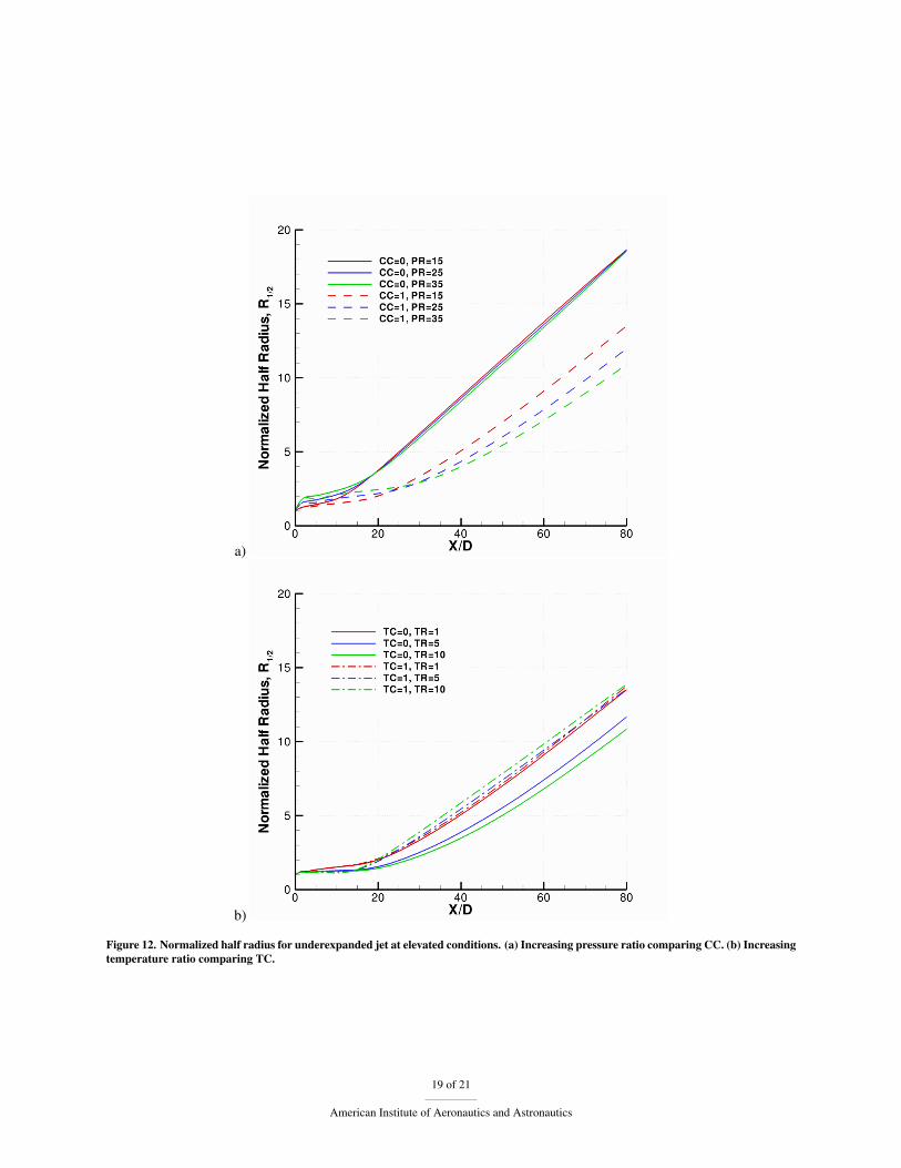
A parametric study is performed using a generic axisymmetric jet setup. The goal is to extrapolate the data tohigher pressure ratios (PR) and temperature ratios (TR), more closely resembling those experienced during actual LASflight conditions. The pressure ratio is increased from the perfectly expanded conditions (PR = 11) to underexpandedratios of 15, 25, and 35. The temperature ratio is successively increased from isothermal to ratios of 5 and 10. Thecompressibility and temperature corrections are examined. A survey of literature showed that there is very littleexperimental data available for verification at these conditions.

Fig. 12a shows the jet half radius for increasing pressure ratios with the compressibility correction disabled (solidline) and enabled (dashed line). Initially, the half radius is largest for the highest pressure ratio. This is occurs becausethe higher pressure ratio causes the flow to expand more closer to the nozzle lip, forming the first barrel shock. Thereis basically no distinction between the different pressure ratios without the compressibility correction after X/D of

7 of 21

American Institute of Aeronautics and Astronautics

20. This is inconsistent with the observation that growth rate should decrease at higher Mach numbers and highlightsthe deficiency of the base turbulence models. For the compressibility correction, as expected, the growth rate for thehigher pressure ratio is decreased. This tends to imply that that the compressibility correction is required to match theflow physics.

Fig. 12b illustrates the jet half radius for increasing temperature ratios when the temperature correction is disabled(solid line) and enabled (dashed line). In both cases, the compressibility correction remains enabled, as this is howthe temperature correction is intended to be used. The increasing temperature ratios lead to an increase in turbulencekinetic energy. From Eq. 1, this increase causes a rise in the turbulence Mach number. In turn, the turbulence dis-sipation is increased and the turbulent mixing is decreased, showing the the smaller spread rate seen in the figure.The use of the temperature correction essentially returns the spread rate to the initial rate, offsetting the effect of thecompressibility correction. Unfortunately, there is no experimental data at these elevated test conditions, so it cannotbe determined which correction accurately models the flow physics. This study does, however, warrant that cautionmust be exercised when using the corrections at conditions for which they have not been validated.

E. Glenn Jet

Finally, comparisons are made for the 3-D Glenn jet with crossflow. Figure 13 shows the velocity magnitudecontours at four downstream locations perpendicular to the freestream, normalized by the jet exit diameter, and com-pared with PIV data. Fig. 14 shows cuts through the middle of the velocity contours to give velocity profiles. For theuncorrected model, the velocity magnitude and vortex roll-up diffuse too quickly when compared with experiment.As seen for the axisymmetric analysis, the compressibility correction shows a large effect on the problem. The veloc-ity magnitude is too high at downstream locations because turbulent mixing in the shear layer is suppressed for toolong. The compressibility correction also shows increased vorticity and thus a shape that is skewed excessively by thevortex roll-up. From this test case, it appears that Sarkar’s model overcorrects by not showing enough mixing withthe freestream. A potential reason for this behavior, when compared with the favorable behavior for the axisymmetricjet, is that the current experiment is performed at much higher turbulent Mach numbers than the previous cases. Thetemperature correction slightly increases the mixing (as before), but does not have a significant effect on the solution.Again, the compressibility correction is dominant for this problem. This is expected because compressibility effectsare large for this flow due to high turbulence Mach numbers in the jet shear layer.

V. Conclusions and Future Work

A. Summary of Key Results

The following summarizes key conclusions and recommendations drawn from the previous analysis:

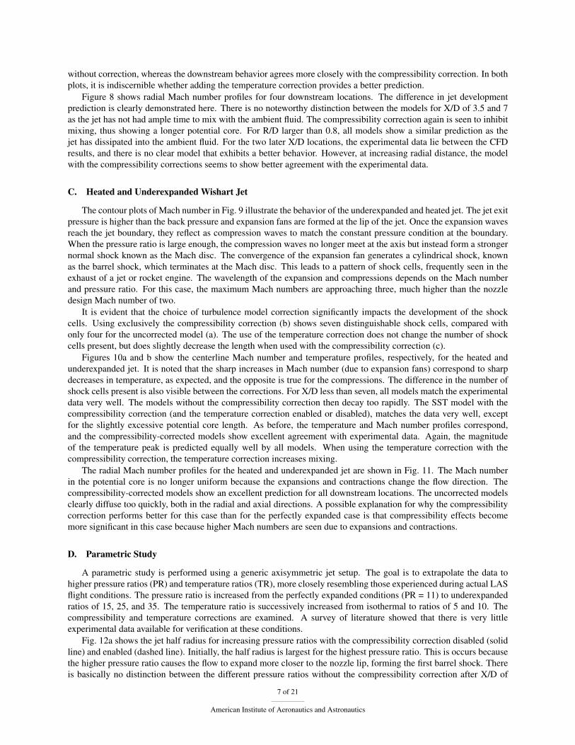
• The SST model is the best choice out of the turbulence models tested for this flow. The k-ω and SA models aretoo diffusive, while the BB model suppresses mixing excessively.

• The use of a compressibility correction is essential for a good prediction of the axisymmetric supersonic jets.While slightly inhibiting mixing in the initial region and thus overpredicting the potential core length, the be-havior in the fully developed region is drastically improved. This improvement is most evident in the accurateprediction of the shock cell structure for the cases with an underexpanded jet.

• The behavior of the temperature correction is not as significant compared to the compressibility correction.For flows in which compressibility effects are significant, the temperature correction should only be used inconjunction with the compressibility correction (as intended when it was formulated by Abdol-Hamid).

• Both the compressibility and temperature corrections must be further evaluated before being used for highertemperature ratios or Mach numbers. The parametric study shows that the effect of the compressibility andtemperature corrections becomes more pronounced at elevated pressure and temperature ratios. The correctionshave not been validated against experimental data at these conditions.

• The 3-D jet with crossflow presents a much more complex flowfield. The physics that must be modeled includevarious vortex interactions between the jet and crossflow. An example is the formation of counter-rotatingvortices which leads to further additional instabilities in the flowfield.

8 of 21

American Institute of Aeronautics and Astronautics

• The compressibility correction by Sarkar does not exhibit sufficient mixing at the higher Mach numbers seenfor the 3-D jet because it suppresses turbulence growth excessively.

• For the 3-D jet, the temperature correction behaves in a manner consistent with the previous axisymmetric jettest cases. Again, it does not have as pronounced an effect as the compressibility correction.

B. Future Work

Examining free shear flows at higher Mach numbers is of interest for future research. Experimental data and directnumerical simulation (DNS) have shown a leveling off in the decrease in shear layer growth rate with increasing Machnumber. This trend is not reflected in current compressibility corrections and may be important when considering flowswhere compressibility effects are even more pronounced. Future work on this project also includes using detachededdy simulation (DES) to model the unsteady pressure loads on the CM surface and to better understand the turbulencein jet flows.

Acknowledgments

This work was supported by NASA JSC under grant NNX09AN06G. The first author would like to thank BrandonOliver, Randy Lillard, Alan Schwing, and Darby Vicker in the Aerosciences and CFD Branch at JSC for all their helpin using OVERFLOW. Also, Robert Childs at NASA Ames was very helpful with questions related to the turbulencemodeling.

References1Nichols, R. H. and Buning, P. G., User’s Manual for OVERFLOW 2.1–Version 2.1t, August 2008.2NASA Constellation Multimedia, [online], http://www.nasa.gov/missionpages/constellation/multimedia/index.html [retreived July 17, 2009].3Eggers, J. E., “Velocity profiles and eddy viscosity distributions downstream of a Mach 2.22 nozzle exhausting into quiescent air,” Tech.

rep., NASA TN D-3601, 1966.4Birch, F. and Eggers, J. E., “A critical review of the experimental data on turbulent shear layers,” Tech. rep., NASA SP 321, 1972.5Lau, J. C., “Measurements in Subsonic and Supersonic Free Jets Using a Laser Velocimeter,” Journal of Fluid Mechanics, Vol. 93, 1979,

pp. 1–27.6Seiner, J. M., Ponton, M. K., Jansen, B. J., and Lagen, N. T., “The Effects of Temperature on Supersonic Jet Noise Emission,” DGLR/AIAA

14th Aeroacoustics Conference, Aachen, Germany, 1992, AIAA Paper 92-02-046.7Sarkar, S., Erlebacher, G., Hussaini, M. Y., and Kreiss, H. O., “The Analysis and Modeling of Dilatational Terms in Compressible Turbu-

lence,” Journal of Fluid Mechanics, Vol. 227, 1991, pp. 473–493.8Georgiadis, N. J., Yoder, D. A., and Engblom, W. A., “Evaluation of Modified Two-Equation Turbulence Models for Jet Flow Predictions,”

44th AIAA Aerospace Sciences Meeting, Reno, Nevada, 2006, AIAA Paper 2006-490.9Abdol-Hamid, K. S., Massey, S. J., and Elmiligui, A., “Temperature Corrected Turbulence Model for High Temperature Flow,” Journal of

Fluids Engineering, Vol. 126, 2004, pp. 844.10Wishart, D. P., The Structure of a Heated Supersonic Jet Operating at Design and Off-Design Conditions, Ph.D. thesis, Department of

Mechanical Engineering, Florida State University, Tallahassee, FL, May 1995.11Gross, N., Assessment of Turbulence Models and Corrections with Application to the Orion Launch Abort System, Master’s thesis, School

of Aeronautics and Astronautics, Purdue University, West Lafayette, Indiana 47907, May 2010.12Wernet, M., Wolter, J. D., Locke, R., Wroblewski, A., Childs, R., and Nelson, A., “PIV Measurements of the CEV Hot Abort Motors Plume

for CFD Validation,” 48th AIAA Aerospace Sciences Meeting, Orlando, FL, 2010, AIAA Paper 2010-1031.13Spalart, P. R. and Allmaras, S. R., “A One-Equation Turbulence Model for Aerodynamic Flows,” 30th AIAA Aerospace Sciences Meeting,

Reno, Nevada, 1992, AIAA Paper 92-0439.14Baldwin, B. S. and Barth, T. J., “A One-Equation Turbulence Transport Model for High Reynolds Number Wall-Bounded Flows,” Tech.

rep., NASA TM 102847, 1990.15Wilcox, D. C., Turbulence Modeling for CFD, DCW Industries, Inc., La Canada, CA 91011, 3rd ed., 2006.16Menter, F., “Two-Equation Eddy-Viscosity Turbulence Models for Engineering Applications,” AIAA Journal, Vol. 32, 1994, pp. 1598–1605.17Zeman, O., “Dilatational Dissipation: The Concept and Application in Modeling Compressible Mixing Layers,” Physics of Fluids, Vol. 2,

1990, pp. 178–188.18Suzen, Y. B. and Hoffmann, K. A., “Investigation of Supersonic Jet Exhaust Flow by One- and Two-Equation Turbulence Models,” 36th

AIAA Aerospace Sciences Meeting, Reno, Nevada, 1998, AIAA Paper 98-0322.

9 of 21

American Institute of Aeronautics and Astronautics

a)

b)

Figure 2. Grid topology for Wishart jet. (a) Overall grid system (showing every 4th grid line), (b) detail view of nozzle lip region.

10 of 21

American Institute of Aeronautics and Astronautics

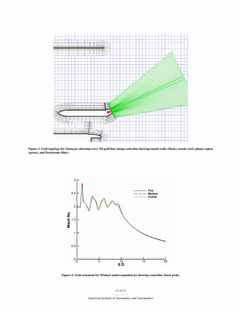
Figure 3. Grid topology for Glenn jet (showing every 5th grid line) along centerline showing tunnel walls (black), nozzle (red), plume region(green), and freestream (blue).

Figure 4. Grid renement for Wishart underexpanded jet showing centerline Mach prole.

11 of 21

American Institute of Aeronautics and Astronautics

a)

b)

Figure 5. (a) Normalized centerline velocity and (b) normalized half radius for Eggers jet comparing turbulence models.

12 of 21

American Institute of Aeronautics and Astronautics

a)

b)

Figure 6. (a) Normalized centerline velocity and (b) normalized half radius for Eggers jet comparing compressibility corrections.

13 of 21

American Institute of Aeronautics and Astronautics

a)

b)

Figure 7. Centerline quantities for heated and perfectly expanded Wishart jet. (a) Mach number, (b) Normalized temperature.

14 of 21

American Institute of Aeronautics and Astronautics

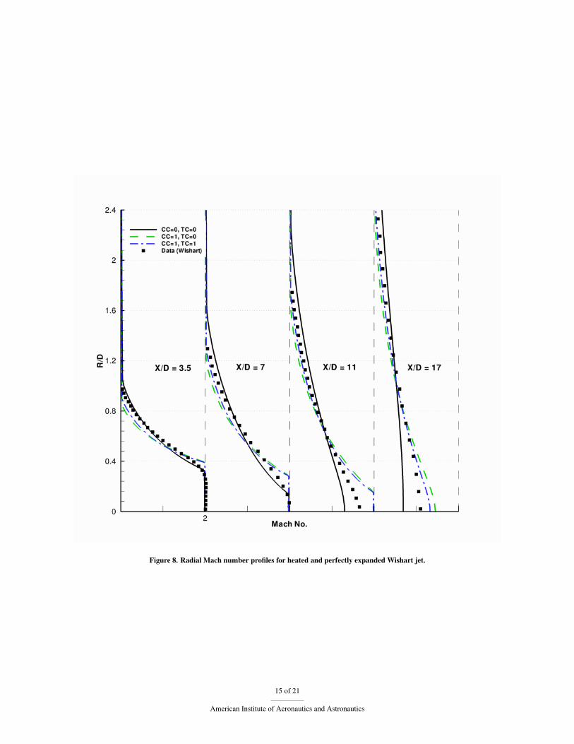
Figure 8. Radial Mach number profiles for heated and perfectly expanded Wishart jet.

15 of 21

American Institute of Aeronautics and Astronautics

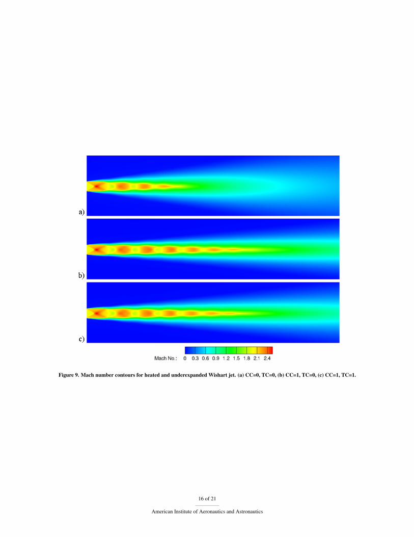
Figure 9. Mach number contours for heated and underexpanded Wishart jet. (a) CC=0, TC=0, (b) CC=1, TC=0, (c) CC=1, TC=1.

16 of 21

American Institute of Aeronautics and Astronautics

a)

b)

Figure 10. Centerline quantities for heated and underexpanded Wishart jet. (a) Mach number, (b) Normalized temperature.

17 of 21

American Institute of Aeronautics and Astronautics

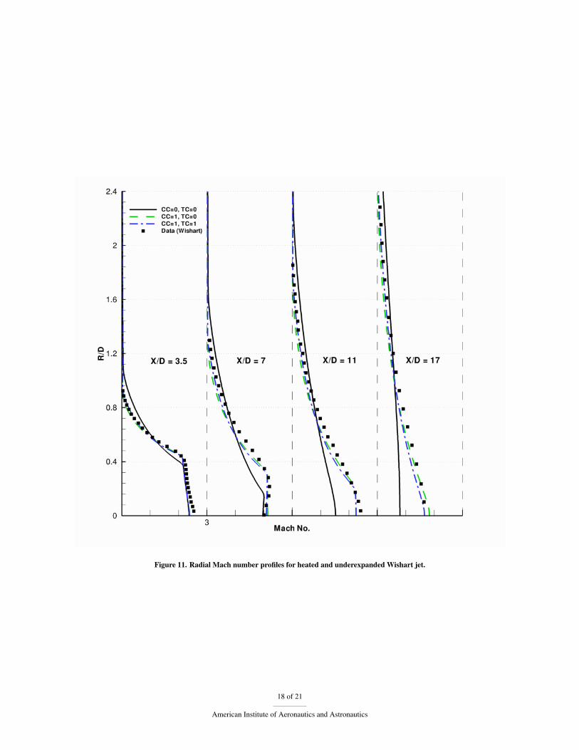
Figure 11. Radial Mach number profiles for heated and underexpanded Wishart jet.

18 of 21

American Institute of Aeronautics and Astronautics

a)

b)

Figure 12. Normalized half radius for underexpanded jet at elevated conditions. (a) Increasing pressure ratio comparing CC. (b) Increasingtemperature ratio comparing TC.

19 of 21

American Institute of Aeronautics and Astronautics

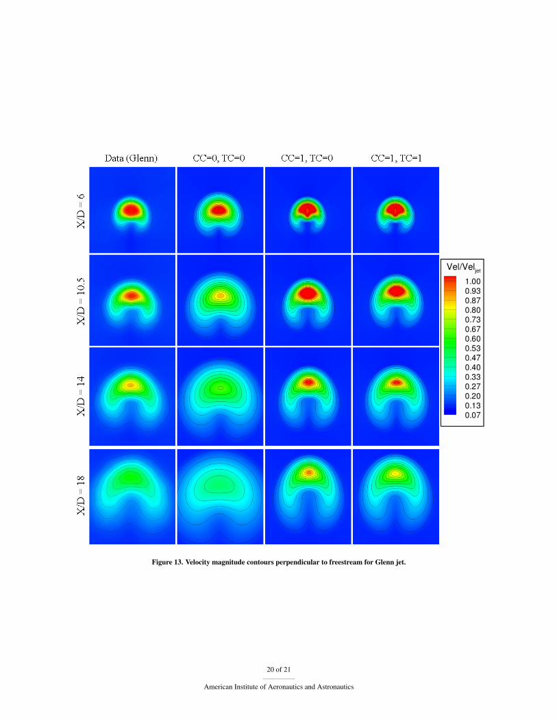
Figure 13. Velocity magnitude contours perpendicular to freestream for Glenn jet.

20 of 21

American Institute of Aeronautics and Astronautics

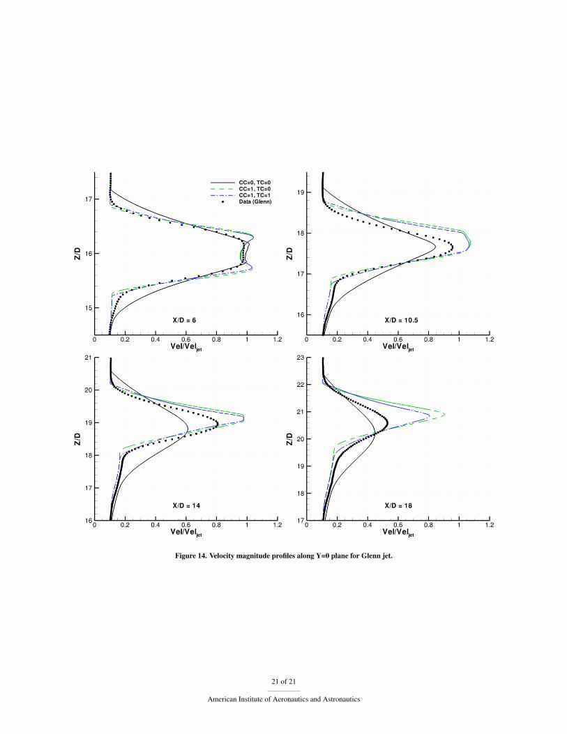
Figure 14. Velocity magnitude profiles along Y=0 plane for Glenn jet.

21 of 21

American Institute of Aeronautics and Astronautics