Methods in Oceanography 17 (2016) 319–334

Contents lists available at ScienceDirect

Methods in Oceanography

journal homepage: www.elsevier.com/locate/mio

Full length article

Observations and parameterizations of surfzonealbedoGregory Sinnett ∗, Falk FeddersenScripps Institution of Oceanography, University of California, San Diego, La Jolla CA 92093, United States

h i g h l i g h t s

• Surfzone albedo can reach 0.45 and varies rapidly with breaking-wave foam.• Image-based parameterization accurately predicts albedo at wave time scales.• Wave-model based parameterization predicts time-averaged cross-shore albedo.

a r t i c l e i n f o

Article history:Received 15 January 2016Received in revised form13 June 2016Accepted 17 July 2016Available online 21 August 2016

Keywords:SurfzoneAlbedoWhitewaterWave breakingParameterization

a b s t r a c t

Incident shortwave solar radiation entering the ocean depends onalbedo α and plays an important role in the temperature variabil-ity and pathogen mortality of the nearshore region. As foam hasan elevated albedo, open-ocean albedo parameterizations includewhitecapping effects through a wind-based foam fraction. How-ever, surfzone depth-limitedwave breaking does not require wind.Surfzone albedo observations are very rare, the variability of surf-zone albedo is not known, and parameterizations are not available.New, year-long upwelling and downwelling shortwave radiationobservations were made from the Scripps Institution of Oceanog-raphy pier spanning the surfzone and inner-shelf. Surfzone albedowas elevated due to foam with mean observed albedo of α = 0.15and one-minute average albedo as high as α = 0.45, far exceedingexpected albedo (0.06) from standard parameterizations. Using apier-mounted GoPro camera, an image-based albedo parameteri-zation is developed that estimates the fractional foam area to de-rive albedo. This parameterization has high skill (r2 = 0.90) ontime scales as short as a wave period (9 s). A second wave-modelbased parameterization for (hourly) averaged albedo is developedrelating the non-dimensional roller energy dissipation to themean

∗ Correspondence to: 9500 Gilman Drive, La Jolla, CA 92093-0209, United States.E-mail address: gsinnett@ucsd.edu (G. Sinnett).

http://dx.doi.org/10.1016/j.mio.2016.07.0012211-1220/© 2016 Elsevier B.V. All rights reserved.

320 G. Sinnett, F. Feddersen / Methods in Oceanography 17 (2016) 319–334

foam fraction and thus albedo. The parameterization has good skill(r2 = 0.68) and resolves cross-shore albedo variations. These newparameterizations can be used where imagery is available or wavemodels are applicable, and can be used to constrain local heat bud-gets and pathogen mortality.

© 2016 Elsevier B.V. All rights reserved.

1. Introduction

The nearshore region (≤ 7mwater depth) is critical both economically and ecologically. The regionis a center for tourism, recreation, and commercial use, and is also home to a wide variety of fish,birds, plants and invertebrates.Water temperature is an important ecological aspect, affecting growthrates, recruitment rates, egg-mass production, pathogen ecology andmany other factors (e.g., Phillips,2005; Fischer and Thatje, 2008; Broitman et al., 2005; Goodwin et al., 2012; Halliday, 2012). In thissensitive region, incident shortwave solar radiation entering the ocean (Qsw) plays an important rolein both the temperature variability (Sinnett and Feddersen, 2014) and pathogen mortality throughUV-B photobiological damage (e.g., Sinton et al., 1994, 2002).

Shortwave solar radiation entering the ocean is defined as

Qsw = Qd − Qu, (1)

where Qd is the total downwelling (downward) component of solar shortwave radiation, and Qu is theupwelling (upward) component of shortwave radiation reflected from the ocean surface. The albedoα (surface reflection coefficient) is defined as

α =Qu

Qd, (2)

making

Qsw = (1 − α)Qd. (3)

Under direct sun, open ocean albedo α depends on the solar zenith angle θs (the angle of sundeclination from vertical) and has a daily average of α ≈ 0.06 (Payne, 1972; Briegleb et al.,1986; Taylor et al., 1996). Under cloudy (diffusely lit) skies, open ocean albedo is near 0.06 and isindependent of θs (Payne, 1972). However, wind generates ocean whitecaps (foam) (e.g., Monahan,1971; Monahan and Muircheartaigh, 1980) associated with elevated albedo. Wind also enhances thesea-surface slope variability (e.g., Ross and Dion, 2007), which affects albedo at large solar zenithangles (e.g., Saunders, 1967). Laboratory measurements indicate that pure foam has albedo α = 0.55(Whitlock et al., 1982). For a fractional surface coverage of foam ζ , the combined effects of foam andopen water on albedo are often (e.g., Koepke, 1984; Frouin et al., 1996; Jin et al., 2011) represented as

α = ζαf + (1 − ζ )αθ , (4)

where αf is the foam albedo, and αθ is the parameterized solar zenith angle dependent open oceanalbedo (e.g., Taylor et al., 1996). The foam fraction ζ from open ocean whitecapping has beenparameterized using a surface wind speed |uw| dependence (e.g., Hansen et al., 1983; Jin et al., 2004,2011), but has a negligible effect on albedo (less than 0.002) for winds |uw| < 12 m s−1 (Payne, 1972;Moore et al., 2000; Frouin et al., 2001).

In the surfzone, foam is generated by depth-limited wave breaking regardless of wind, potentiallyelevating surfzoneα and reducingQsw. Nearshore temperature evolution (e.g., Sinnett and Feddersen,2014; Hally-Rosendahl et al., submitted for publication) depends strongly on Qsw in the surfzone andinner-shelf, the region just seaward of the surfzone. Elevated surfzone albedo may also help explainreduced surfzone pathogenmortality relative to the inner-shelf (e.g., Rippy et al., 2013a,b)making the

G. Sinnett, F. Feddersen / Methods in Oceanography 17 (2016) 319–334 321

Fig. 1. (a) Photo of the Scripps Institution of Oceanography (SIO) pier (La Jolla, California) and nearshore region at low tide.(b) Mean cross-shore bathymetric profile with mean tide level and approximate tidal extents. The radiometer is located atxR = −100 m (indicated with an orange marker), a location frequently within the surfzone.

surfzone albedo an important factor controlling the ecology of the region. Limited (21 min) surfzonealbedo observations at 440–650 nmwavelengths reported elevated albedo up to 0.4–0.6, compared to0.06 observed in the inner-shelf (Frouin et al., 1996), potentially influencing the surfzone heat budget(Sinnett and Feddersen, 2014). However, no other surfzone albedo observations have been published(to our knowledge) and depth-limited wave-breaking albedo parameterizations do not exist. Thus,the magnitude and variability of surfzone albedo are not known, nor are its impacts on nearshoretemperature and pathogen mortality. Making surfzone albedo observations is difficult, thus surfzonealbedo parameterizations are needed.

Results from a year-long experiment at the Scripps Institution of Oceanography (SIO) pier measur-ing nearshore albedo under awide variety of conditions are presented here, together with tests of twosurfzone albedo parameterizations. As surfzone foam is visible in both time-elapsed (e.g., Lippmannand Holman, 1990; Holland et al., 1997; Almar et al., 2010) and snapshot (e.g., Stockdon and Holman,2000; Chickadel et al., 2003) optical images, the first parameterization uses optical images to estimatefoam fraction and albedo. The second parameterization uses a wave and roller transformation modelto estimate foam fraction and albedo. The experimentmethods and observations are described in Sec-tion 2. Results and the two parameterizations are presented in Section 3, discussed in Section 4, andsummarized in Section 5.

2. Methods and observations

2.1. Experiment description

Shortwave solar radiation, wave statistics, winds, and water depth were measured betweenOctober 25th, 2014 and October 25th, 2015 at the SIO pier (Fig. 1(a)), La Jolla, California (lat 32.867,lon −117.257). Cross-shore (x) bathymetry profiles were made at 0.5 to 1 month intervals (see dotsin Fig. 3(a)) between x = 0 m (the cross-shore location of the shoreline extents at mean tide at thestart of the experiment) and the pier end at x = −270m. NOAA tide gauge station 9410230 at the SIOpier end (in ≈7 m water depth) measured the water level at 6 min intervals. A representative cross-sectional view (Fig. 1(b)) shows the mean bathymetric profile, the Mean Tide Level (MTL) referenceheight (h = 0), and tidal standard deviation (≈0.5 m).

Downwelling, Qd and upwelling, Qu shortwave solar radiation was measured by a CampbellScientific NR01 research grade four-way radiometer (Fig. 2(b)) having two shortwave radiationsensors (wavelengths from 305 nm to 2800 nm) with 2.9 s response time and cosine angle spatialresponse over a 180° field of view. The sensor noise level is <1.5% of the signal, instrument drift isexpected to be <1% per year, and instrument tilt errors are expected to be <2%. Both radiometersensors were calibrated within one year of their deployment according to ISO 9847.

322 G. Sinnett, F. Feddersen / Methods in Oceanography 17 (2016) 319–334

Fig. 2. (a) Photo of the Campbell Scientific NR01 radiometer deployed over the surfzone, mounted on the south side of theSIO pier. (b) A close-up of the NR01 radiometer, consisting of upwelling and downwelling shortwave radiation sensors. (c) Aschematic of the boom mount allowing radiometer deployment 6.5 m above MTL at a distance 6.35 m from the pier pilings.Hinges (arrows) allow the boom to pivot laterally and swing vertically for regular radiometer cleaning.

The NR01 radiometer was attached to the end of a custom designed boom arm (Fig. 2(b)) and fittedto the south side of the SIO pier at xR = −100 m. The cross-shore deployment location was chosen sothat the radiometerwould observe the surfzone roughly two-thirds of the time depending on the tidaldepth andwave height. The radiometer wasmounted 6.5m aboveMTL to avoid significant spray frombreaking waves, while assuring that more than 90% of the upwelling signal was confined to a 14 mradius watch circle beneath the instrument. The mounting boomwas hinged at the pier end andmid-boom arm (Fig. 2(c) arrows) allowing it to swing parallel and pivot up to the pier deck for cleaning atroughly 5 day intervals.

Generally, the radiometer sampled Qd and Qu continuously at 1 Hz, storing the 1 min mean andstandard deviation. On 9 days, a GoPro camera with a 72° vertical and 94° horizontal field of viewwasmounted on the pier deck approximately 2.5 m above the radiometer looking down at the water at≈45° from horizontal. The camera captured images of the surfzone conditions at two second intervalswith a 1/4000 s shutter speed, f/2.8 aperture value and ISO 100 speed rating. During this time theradiometer stored 1 Hz samples directly, allowing image and albedo comparison.

At pier-end, hourly significant wave height H(p)s and peak period Tp were estimated by the Coastal

Data Information Program wave gauge. During times when the wave gauge was offline (July 29 toAugust 20, 2015) a realtime spectral refraction wave model initialized from offshore buoys (O’Reillyand Guza, 1991, 1998) with very high skill was used.Winds were observed by the NOAA station at thepier end 18 m above MTL and reported as six-minute averaged values. The experiment site latitudeand local time were used to calculate solar zenith angle θs based on Reda and Andreas (2008).

2.2. Observations

At xR, the water depth hR varied due to tidal changes in sea surface elevation and on longer timescales due to bathymetry changes (Fig. 3(a)). Beach profile evolution followed a wintertime (definedhere as day 26 on November 20, 2014 to day 126 on February 28, 2015) erosion and summertime (day212 on May 25, 2015 to day 312 on September 2, 2015) accretion pattern, characteristic of southernCalifornia beaches (e.g., Ludka et al., 2015).

Pier-end significant wave height H(p)s varied between 0.22 m and 2.16 m and peak period Tp

between 3 s and 18 s (not shown) with increased wave activity occurring every few days, modulated

G. Sinnett, F. Feddersen / Methods in Oceanography 17 (2016) 319–334 323

Fig. 3. Hourly time-series over the year-long experimental period of (a) water depth hR at the radiometer cross-shore location(xR = −100m), (b) pier-end significant wave heightHs , (c) wind speed |uw|, (d) solar zenith angle θs , (e) observed downwellingQd (red) and upwelling Qu (blue) short-wave solar radiation, and (f) observed albedo αo = Qu/Qd . Times when Qd or Qu werecorrupted are removed in (e) and (f). (For interpretation of the references to color in this figure legend, the reader is referred tothe web version of this article.)

seasonally with typically stronger wintertime and weaker summertime wave events (Fig. 3b). Windswere typically calm, with average wind speed |uw| of 2.25 m s−1 having diurnal variability andoccasional peaks above 10 m s−1, particularly in winter (Fig. 3(c)). Solar zenith angle fluctuateddiurnally with daily minimum θs varying on an annual time-scale between 56.31° and 9.43° nearthe winter and summer solstice respectively (Fig. 3(d)).

Foam-free albedo depends on θs in direct light (clear sky) but not in diffuse light (cloudy skies)(Payne, 1972). Lighting conditions are characterized with the atmospheric transmittance Tr definedas the ratio of the observed downwelling radiation Qd to the theoretical maximum Qd,

Tr =Qd

S cos(θs)γ −2, (5)

where S is the solar constant and γ is the ratio of the actual to mean earth–sun separation distance.Direct light conditions are defined when Tr > 0.6, and diffuse light conditions are defined when Tr <0.3. The observations weremade in 58% clear sky, 16% cloudy sky and 26%mixed sky (0.3 < Tr < 0.6)conditions.

Both Qd and Qu observations were removed during rain or heavy fog events when the radiometerwas affected by moisture. In addition, Qd and Qu observations were removed when θs > 60° toavoid nighttime and times when the sun was behind a coastal bluff or very near the horizon. The

324 G. Sinnett, F. Feddersen / Methods in Oceanography 17 (2016) 319–334

radiometerwas too close to the cross-shore location of exposed sandwhen, at xR, the depthhR < 1.3m(approximately 38% of the time). These observations were also removed. The boom arm extended6.35 m to the south of the pier to avoid pier shadow under clear skies, when the vast majority oflight arrives from the southern sky. However, when the solar azimuth angle φ < 109° (<0.1% ofthe time), pier shadows were cast under the radiometer and these observations were removed. Intotal, ≈50% of daytime data was retained. For pure diffuse light conditions, the true Qu is slightlyunderestimated primarily due to pier deck shadow reducing the available downwelling light and alsodue to pier pilings directly blocking a fraction of the upwelling light from the north. This effect iscorrected following Payne (1972) so that the upwelling shortwave radiation is

Qu = Qmu[1 + 0.15(1 − Tr)], (6)

where Qmu is the measured upwelling shortwave radiation, Tr is the atmospheric transmittance, andpier geometry sets the coefficient (0.15). This correction has no effect on the results.

Downwelling shortwave radiation Qd had a predominantly diurnal pattern with seasonal long-term variability and short (<6 h) time-scale variability due to clouds (red in Fig. 3(e)). Clear-skydaily maximum Qd varied between 610 W m−2 in wintertime to 1064 W m−2 in the summer.Clouds typically reduced Qd, but also increased Qd for short periods (seconds to minutes) due tomagnification caused by the ‘‘edge-of-cloud’’ effect (e.g., Davies, 1978; Coakley and Davies, 1986).Reflected shortwave upwelling radiation Qu (blue in Fig. 3(e)) also varied on diurnal time scales, butcontained variability on shorter time scales as well. A time series of over 70,000 one-minute averagedobserved albedo observationsαo was generated from the retainedQd andQu with (2). Observed albedoαo varied from 0.04 to 0.45 on a range of timescales from minutes to many days (Fig. 3(f)).

3. Results

3.1. Albedo dependence on θs and waves

Here, the one-minute averaged observed albedo αo is directly compared to solar zenith angle (θs)dependent parameterizations that assume no foam (e.g., Taylor et al., 1996). Observed one-minuteaveraged albedo αo are significantly elevated from a solar zenith angle dependent parameterizationαθ (compare dots to red dashed in Fig. 4) for both clear and diffuse light conditions. For cos |θs| > 0.5,αo varied from near 0.04, typical of αθ , to 0.45, far exceeding αθ (Fig. 4). Over all conditions spanningboth the surfzone and inner-shelf, themean albedowas 0.11, nearly twice previous estimates of open-ocean daily averaged albedo (e.g., Payne, 1972). Although theminimum αo values are consistent withαθ under both light conditions, the binned mean αo is roughly one αo standard deviation higher thanαθ for all θs in both clear and diffuse light conditions (compare red diamonds and vertical bars to reddashed curve, Fig. 4).

Depth-limited wave breaking is often well determined by the ratio of local wave height to waterdepthHs/h (e.g., Thornton andGuza, 1983). To investigatewhether the elevatedαo is due to breaking-wave generated foam or rather due to surface wind speed (as in open ocean parameterizations), therelationship between ⟨αo⟩ (where ⟨⟩ denotes an hourly average) and H(p)

s /hR is examined, where H(p)s

is the pier-end (x = −270 m) significant wave height and hR is the water depth at the radiometer(xR = −100 m). Hourly-averaged ⟨αo⟩ varies between 0.04–0.33 and is strongly related to H(p)

s /hR(Fig. 5(a)) with r2 = 0.64. Wind speeds at this location were typically weak; mean winds were≈2 m s−1, and sustained winds over 4 m s−1 were observed less than 12% of the time. As expected,winds were not correlated with ⟨αo⟩ (Fig. 5(b)) since total ocean reflectance when winds are lessthan 8 m s−1 is negligible (Koepke, 1984) and whitecapping due to winds below 15 m s−1 has notbeen observed to enhance albedo (Payne, 1972; Frouin et al., 2001). The relationship between ⟨αo⟩

and H(p)s /hR demonstrates that for larger incident waves H(p)

s or smaller local water depth hR, ⟨αo⟩ iselevated in a consistent manner and confirms that the breaking-wave foam strongly contributes tothe observed albedo, motivating the following two parameterization approaches.

G. Sinnett, F. Feddersen / Methods in Oceanography 17 (2016) 319–334 325

Fig. 4. One-minute averaged observed albedo αo versus cos(θs) under (a) clear sky conditions (Tr > 0.6) and (b) diffuse lightconditions (Tr < 0.3). Binnedmeans (red diamonds) and± one standard deviation (red vertical lines) of αo aremostly elevatedover the θs-only based Taylor et al. (1996) parameterization αθs (red dashed). (For interpretation of the references to color inthis figure legend, the reader is referred to the web version of this article.)

Fig. 5. Hourly averaged observed albedo ⟨αo⟩ versus (a) hourly-observed H(p)s /hR where H(p)

s is the significant wave heightmeasured at the pier-end (x = −270 m) and hR is the water depth at the radiometer, and (b) hourly averaged wind speed.Correlation between albedo and wind speed at this site (r2 = 0.06) is not significant from zero at the 95% confidence interval,however albedo is correlated with H(p)

s /hR (r2 = 0.64).

3.2. Image-based parameterization

Following open-ocean whitecapping parameterizations (e.g., Hansen et al., 1983; Jin et al., 2004,2011), surfzone albedo is expected to depend on θs and the breaking-wave generated foam fractionζw. Time-averaged and snapshot images of the surfzone have successfully been used to identify areaswith elevated foam (e.g., Lippmann and Holman, 1990; Stockdon and Holman, 2000). Here, imagesfrom the pier-mounted GoPro camera are used to estimate ζw and compared to 1-Hz sampled αo toderive an image-based albedo parameterization.

For a broken wave with extensive foam (Fig. 6(a)), the 1-Hz sampled αo = 0.33, elevated aboveαθ = 0.06. In contrast, for foam-free conditions (Fig. 6(b)), αo = 0.05, consistent with expected αθ .The images were cropped and converted to 0–255 count grayscale G (Fig. 6(c) and (d)) representingthe ocean surface light intensity. The grayscale value G = 0.2989r + 0.5870g + 0.1140b, where r , band g are the red, blue and green components respectively, retain luminance while removing hue andsaturation. Elevated G can result from foam (white areas in Fig. 6(c)) or sun glint (specular reflection,

326 G. Sinnett, F. Feddersen / Methods in Oceanography 17 (2016) 319–334

0 50 100 150 200 250

Grayscale Value (G)

0 50 100 150 200 250

Grayscale Value (G)

0.03

0.02

0.01

0

Fig. 6. Images of water below the radiometer (a) during a breaking event when αo = 0.33 and (b) under calm non-breakingconditions when αo = 0.05. Cropped and grayscale converted images of (c) a breaking wave and (d) non-breaking. PDFs ofthe grayscale values for (e) breaking conditions and (f) non-breaking conditions are delineated (vertical black lines) to showgrayscale pixel values classed as ‘‘open water’’ (G < 170), ‘‘foam’’ (170 < G < 230) and ‘‘sun glint’’ (G > 230). The fraction ofpixels identified as ‘‘foam’’ (ζw) is 0.55 under breaking conditions (left), but only 0.03 for non-breaking conditions (right).

upper left Fig. 6(d)). Typically, sun glint is brighter than foam, which is brighter than foam-free areas,allowing for differentiation between regions using grayscale values.

For the breaking case, the probability density function (PDF) of grayscale pixel values p(G) containsthree peaks near 100, 190 and 255 (Fig. 6(e)), corresponding to areas of open water, foam and sunglint in Fig. 6(a). For the non-breaking case, p(G) only has two peaks near 100 and 255 (Fig. 6(d))corresponding to open water and sun glint. The peak near 190 associated with foam (Fig. 6(c)) is notpresent. To quantify image area containing open water, foam and sun glint, all grayscale PDFs are firstaveraged together forming a mean p(G) (not shown). Similar to Carini et al. (2015), PDF curvaturep′′(G) maxima define cutoff values between open water, whitewater and sun glint (lines on Fig. 6(e),(f)), here found to be G = 170 and G = 230. As foam is not a specular reflector (Monahan et al., 1986),sun glint must be from foam free regions and is thus classified as open water. The pixel fraction (as aproxy for surface area) of foam ζw is then calculated. For the breaking case (Fig. 6(e)), the pixel fractionattributed to foam was ζw = 0.55, and for the non-breaking case (Fig. 6(f)) ζw = 0.03. This approachis applied to all images, creating a time series of foam fraction ζw(t) at xR.

Similar to open ocean whitecapping albedo formulations (4), the image-derived albedo αI is

αI = ζwαf + (1 − ζw)αθ , (7)

where αθ is the θs dependent parameterization for foam-free water, ζw is derived from the images,and the foam albedo αf is considered a free parameter. The 1-Hz αo varied over 0.02–0.45, spanninga broad range of solar zenith angle (13.7° < θs < 56°), depth (1.3 < h < 2.6 m) and wave height(0.45 < Hs < 1.21 gm) conditions. Minimizing the rms error between αI and αo results in a bestfit αf = 0.465 and a surfzone albedo parameterization with high skill (r2 = 0.90 with binned-meanr2 = 0.97, Fig. 7).

G. Sinnett, F. Feddersen / Methods in Oceanography 17 (2016) 319–334 327

Fig. 7. Gridded logarithmic density (gray scale) of image-derived albedo αI versus observed albedo αo sampled at 1 Hz for ninedays (N = 137, 547). The observations were made when θs varied between 13.7° and 56°, depth h varied between 1.3 m and2.6 m, and pier-end Hs varied between 0.45 m and 1.21 m. The best fit αf = 0.465 has fit skill r2 = 0.90 with binned mean(red diamonds) fit skill r2 = 0.97. Binned-mean standard deviations are represented by red lines. Bins contained at least 100observations. (For interpretation of the references to color in this figure legend, the reader is referred to the web version of thisarticle.)

The high skill of the parameterized αI is highlighted with a ten-minute example including severalbreaking wave events from larger wave-groups at 1–2 min intervals (Fig. 8). Breaking waves causedobserved albedo αo (black line, Fig. 8) to increase sharply (in a few seconds), well above αθ (blackdotted). Individual αo peaks during a large wave-group event (around 200 s) were spaced nearTp = 9 s. The highest αo values, near 0.35, occurred after two or more successive breaking wavesalmost completely covered the radiometer’s field of view. Smaller αo peaks occurred when breakingevents partially filled the field of view or did not break as vigorously. After the initial step-like increaselasting a few seconds, the albedo decayed toward αθ with time scales ≈20 s as the bubbly foamoutgassed (e.g., Ma et al., 2011). The asymmetry of the observed albedo αo rapid increases and sloweroutgassing decay are well represented by αI (red curve, Fig. 8), and αI tracks αo at both wave groupand individual-wave timescales. At αo peaks (particularly>0.2), after a rapid increase, parameterizedαI tends to have a high bias (Fig. 8). This elevated αI bias for αo > 0.2 is also seen in the scatterplot(Fig. 7) and is discussed further in Section 4. Overall this image-based parameterization predicts thefoam-induced elevated αo unexplained by αθ (Fig. 4), and the good αI and αo time-series agreement(Fig. 8) is also seen at other times and over a wide variety of surfzone conditions.

3.3. Wave model based albedo parameterization

Although the image-based parameterization has very high skill, a camera is required,which often isnot available. However, given knowledge of one dimensional h(x), wave transformation models havehigh skill in predicting the cross-shore evolution ofwave height (e.g., Ruessink et al., 2001, 2003). Thismotivates a second albedo parameterization that utilizes a wave model to relate roller dissipation tofoam fraction and albedo through (4).

Assuming normally-incident narrow-banded waves on alongshore uniform beaches, one-dimensional wave and roller transformationmodels (e.g., Thornton and Guza, 1983; Battjes and Stive,1985; Ruessink et al., 2001) relate wave energy flux gradient to wave-energy dissipation,

ddx

(ECg) = −⟨ϵb⟩, (8)

328 G. Sinnett, F. Feddersen / Methods in Oceanography 17 (2016) 319–334

Fig. 8. Ten-minute time series of image-derived albedo αI (red), observed albedo αo (black) and parameterized open oceanalbedoαθ (dashed) beginning near noon on September 11, 2015.Water depth h(xR) = 1.5mwithmoderatewaves (Hs = 0.6mand Tp = 9 s at the pier-end) and light winds (|uw| = 3.7 m s−1) with θs = 31°. (For interpretation of the references to colorin this figure legend, the reader is referred to the web version of this article.)

where E is the wave energy density, Cg is the group velocity given by linear theory, and ⟨ϵb⟩ is thebulk breaking wave dissipation. The wave energy density is E = 1/16ρgH2

s where ρ is water density,g is gravity and Hs is the local significant wave height. The breaking wave dissipation ⟨ϵb⟩ is given byChurch and Thornton (1993) with standard breaking parameters (B = 0.9 and γ = 0.57). The rollerenergy equation is (e.g., Ruessink et al., 2001)

ddx

(2Erc) = −⟨ϵr⟩ + ⟨ϵb⟩, (9)

where Er is the roller energy density and c is the linear theory phase speed. Roller dissipation is definedas (Deigaard, 1993)

⟨ϵr⟩ =2gEr sinβ

c(10)

with slopeβ = 0.1 (e.g., Walstra et al., 1996). The coupled Eqs. (8) and (9) are solvedwith the specifiedh(x) and offshore (pier-end) boundary conditions of observed Hs and Tp, with Er = 0.

Example output from the wave and roller model characterizes the cross-shore evolution of Hs(Fig. 9(a)) due to the bathymetric profile (Fig. 9(e)). As waves shoal onshore, wave height increasesto Hs = 1.5 m at x = −170 m where breaking occurs, roller dissipation becomes non-zero (Fig. 9(b))and wave height decreases. The terraced, non-monotonic bathymetry create undulating regions ofelevated ⟨ϵr⟩ (e.g., near x = 140 m, x = 90 m, Fig. 9(b)) and weaker ⟨ϵr⟩ (e.g., near x = 125 m andx = 65 m).

To develop a wave-model based albedo parameterization αw, the average foam fraction ⟨ζw⟩ ishypothesized to depend linearly on non-dimensional () wave roller dissipation ⟨ϵr⟩ as

⟨ζw⟩ = m⟨ϵr⟩, (11)

where ⟨ϵr⟩ is non-dimensionalized by wave-dissipation scaling (e.g., Battjes, 1975; Feddersen andTrowbridge, 2005; Feddersen, 2012a,b) as

⟨ϵr⟩ =⟨ϵr⟩

ρ(gh)3/2, (12)

andm is a fit parameter foundbyminimizing rms error betweenαo andαw. The hourly averagedwave-model based albedo is found from (4) using ⟨ζw⟩ and αf = 0.465 as in Section 3.2. The radiometerobserved αo is a cosine angle weighted area-average with ≈ 14 m radius. To compare the observed

G. Sinnett, F. Feddersen / Methods in Oceanography 17 (2016) 319–334 329

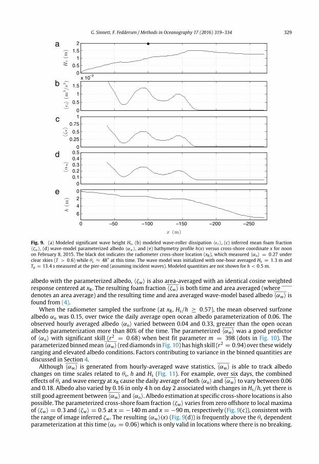
Fig. 9. (a) Modeled significant wave height Hs , (b) modeled wave-roller dissipation ⟨ϵr ⟩, (c) inferred mean foam fraction⟨ζw⟩, (d) wave-model parameterized albedo ⟨αw⟩, and (e) bathymetry profile h(x) versus cross-shore coordinate x for noonon February 8, 2015. The black dot indicates the radiometer cross-shore location (xR), which measured ⟨αo⟩ = 0.27 underclear skies (T > 0.6) while θs ≈ 48° at this time. The wave model was initialized with one-hour averaged Hs = 1.3 m andTp = 13.4 s measured at the pier-end (assuming incident waves). Modeled quantities are not shown for h < 0.5 m.

albedo with the parameterized albedo, ⟨ζw⟩ is also area-averaged with an identical cosine weightedresponse centered at xR. The resulting foam fraction ⟨ζw⟩ is both time and area averaged (wheredenotes an area average) and the resulting time and area averaged wave-model based albedo ⟨αw⟩ isfound from (4).

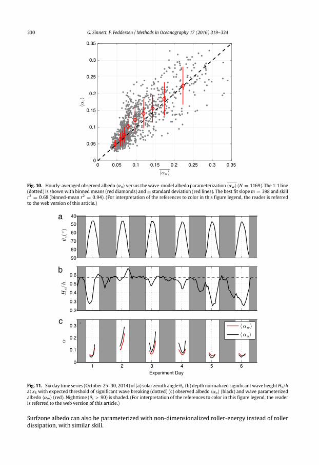
When the radiometer sampled the surfzone (at xR, Hs/h ≥ 0.57), the mean observed surfzonealbedo αo was 0.15, over twice the daily average open ocean albedo parameterization of 0.06. Theobserved hourly averaged albedo ⟨αo⟩ varied between 0.04 and 0.33, greater than the open oceanalbedo parameterization more than 80% of the time. The parameterized ⟨αw⟩ was a good predictorof ⟨αo⟩ with significant skill (r2 = 0.68) when best fit parameter m = 398 (dots in Fig. 10). Theparameterized binnedmean ⟨αw⟩ (red diamonds in Fig. 10) has high skill (r2 = 0.94) over thesewidelyranging and elevated albedo conditions. Factors contributing to variance in the binned quantities arediscussed in Section 4.

Although ⟨αw⟩ is generated from hourly-averaged wave statistics, ⟨αw⟩ is able to track albedochanges on time scales related to θs, h and Hs (Fig. 11). For example, over six days, the combinedeffects of θs and wave energy at xR cause the daily average of both ⟨αo⟩ and ⟨αw⟩ to vary between 0.06and 0.18. Albedo also varied by 0.16 in only 4 h on day 2 associated with changes in Hs/h, yet there isstill good agreement between ⟨αw⟩ and ⟨αo⟩. Albedo estimation at specific cross-shore locations is alsopossible. The parameterized cross-shore foam fraction ⟨ζw⟩ varies from zero offshore to local maximaof ⟨ζw⟩ = 0.3 and ⟨ζw⟩ = 0.5 at x = −140 m and x = −90 m, respectively (Fig. 9(c)), consistent withthe range of image inferred ζw. The resulting ⟨αw⟩(x) (Fig. 9(d)) is frequently above the θs dependentparameterization at this time (αθ = 0.06) which is only valid in locations where there is no breaking.

330 G. Sinnett, F. Feddersen / Methods in Oceanography 17 (2016) 319–334

Fig. 10. Hourly-averaged observed albedo ⟨αo⟩ versus thewave-model albedo parameterization ⟨αw⟩ (N = 1169). The 1:1 line(dotted) is shownwith binnedmeans (red diamonds) and± standard deviation (red lines). The best fit slopem = 398 and skillr2 = 0.68 (binned-mean r2 = 0.94). (For interpretation of the references to color in this figure legend, the reader is referredto the web version of this article.)

Fig. 11. Six day time series (October 25–30, 2014) of (a) solar zenith angle θs , (b) depth normalized significantwave heightHs/hat xR with expected threshold of significant wave breaking (dotted) (c) observed albedo ⟨αo⟩ (black) and wave parameterizedalbedo ⟨αw⟩ (red). Nighttime (θs > 90) is shaded. (For interpretation of the references to color in this figure legend, the readeris referred to the web version of this article.)

Surfzone albedo can also be parameterized with non-dimensionalized roller-energy instead of rollerdissipation, with similar skill.

G. Sinnett, F. Feddersen / Methods in Oceanography 17 (2016) 319–334 331

4. Discussion

Elevated surfzone albedo can impact heat budgets (Sinnett and Feddersen, 2014) and pathogenmortality (e.g., Sinton et al., 2002). Water-entering short-wave solar radiation Qsw is the largestsurfzone heat budget term (Sinnett and Feddersen, 2014). An average surfzone albedo increase fromα = 0.06 to (as observed) α = 0.15 would reduce Qsw so that cross-shore advection or waveheating are relatively more important. For example, Sinnett and Feddersen (2014) found a residualsurfzone heat export of 5.2 × 103 W m−1. Revising the heat budget using α = 0.15, reducesthe residual heat export by 30%. Dye tracer can linger in the surfzone for >12 h (Hally-Rosendahlet al., submitted for publication), indicating the time-scales pathogens can remain in bathing waters.Increasing albedo from 0.06 to 0.15 roughly doubles fecal coliform bacterial survival rates (Sintonet al., 2002), increasing potential human health risk if not appropriately accounted for.

The observed albedo αo is a space and time-average over the radiometer’s 14-m radius cosineresponse and 2.9 s time constant. With propagating breaking waves which continuously outgasbubbles, the radiometerwill never instantaneously sample pure foam over its entire field of view. Thismay explain why the best-fit foam albedo αf = 0.465 is less than the laboratory observed maximumvalue of 0.55 (Whitlock et al., 1982). Although the image-based αI predicts αo with high skill (Fig. 7),for αo > 0.2, αI is biased high particularly when a breaking wave front passes and dα/dt is large(Fig. 8). The 2.9 s radiometer response time, relative to the near-instantaneous camera response time,may explain this bias at times of step function-like changes in albedo.

The specific grayscale PDF cutoff limits for open water, foam, and sun glint, derived from p′′(G)extrema, are the result of the lighting and fixed camera settings at this location. To apply thisparameterization with another camera or at another location, one must first establish the relevantp′′(G) based cutoff limits. This method can also be applied to time-averaged images. Good agreementbetween αI and αo was found with a constant foam albedo αf applied to grayscale values within thefoam cutoff limits. The fit may be improved if αf is a function of G. Furthermore, images were notgeorectified. The images were cropped to limit the field of view to a relatively small area beneath theradiometer, and the 45° camera angle caused the imaged pixel area to have a similar spatial responseas the radiometer. For example, the pixels near the top of the image cover roughly 35%more area thanthe pixels near the bottom, and the radiometer cosine response reduces the signal by roughly 40% nearthe top of the image. As the camera and radiometerwere samplingwith similar spatial weights, imagerectification was not needed. However, image rectification may be required if this parameterizationtechnique is applied to images covering a wider area (e.g., ARGUS), or to images taken at shallowerangles.

When breaking occurs, ⟨αo⟩ is elevated above αθ (Figs. 3 and 4), and the wave-model basedparameterizationhas good skill (r2 = 0.68) in predictingαo (Fig. 10), although significant unexplainedvariance remains. Waves were assumed to be normally-incident (as expected for long-period wavesin h < 6 m), and standard wave and roller model coefficients were used. The bathymetry nearpiers is often scoured (Elgar et al., 2001), which may result in pier-based bathymetry measurementerrors. Depth h errors and wave model errors would induce roller energy dissipation ⟨ϵr⟩ errors, andeventually ⟨αw⟩ errors, potentially contributing to the unexplained variance in Fig. 10.

5. Summary

Breaking-wave induced foam elevates albedo α relative to foam-free ocean. Open-ocean albedoparameterizations account for foam through a wind speed dependent whitecapping foam fractionζw. However, surfzone depth-limited wave breaking does not depend on wind, and wind-based foamfraction parameterizations are inaccurate in the surfzone. Measuring albedo in the energetic surfzoneenvironment is difficult, and observations of surfzone albedo are very rare. The variability of surfzonealbedo is not known, and parameterizations have not been available. Ocean-entering shortwave solarradiation Qsw depends on albedo and affects both temperature variability and pathogen mortality.This motivates new observations of surfzone albedo and the development of two surfzone albedoparameterizations based on camera images and a wave model.

332 G. Sinnett, F. Feddersen / Methods in Oceanography 17 (2016) 319–334

A year-long experiment at the Scripps Institution of Oceanography pier observed upwelling Quand downwelling Qd shortwave radiation spanning the surfzone and inner-shelf over a range ofwave and depth conditions. A two-way radiometer was mounted 6.5 m above the mean oceansurface and 6.35 m away from the pier, limiting pier shadow effects. Additional wave, wind, tidaland bathymetric observations were collected. On nine days, a downward-looking GoPro camera fixedabove the radiometer location continuously captured water surface images. For solar zenith angleθs < 60°, one-minute averaged observed albedo (as large as αo = 0.45) far exceeded the open oceansolar zenith angle parameterized albedo of 0.06. The elevated observed albedowas related to breakingwave conditions under the radiometer and observed albedo was not related to the wind speed.

A surfzone albedo parameterization is developed using images to estimate foam fraction ζw,identified by the distribution of grayscale pixels values. This image-based parameterization has highskill (r2 = 0.90), with a best-fit parameter for foam albedo of αf = 0.465, slightly less than laboratorymaximum of 0.55 likely due to radiometer finite time and spatial response. This parameterizationcaptures albedo variability on the time-scales of individual waves (9 s) and wave groups (minutes).

Awave-model based parameterization relates non-dimensionalizedwave roller energy dissipationto the hourly-averaged foam fraction ⟨ζw⟩ and, thus, to albedo. The wave model is initiatedwith bathymetry and incident wave conditions. This parameterization predicts hourly averagedobservations from the radiometer, has good skill (r2 = 0.68), and can resolve cross-shorealbedo variations. Bathymetry or wave model errors may contribute to unexplained variance. Thesenew parameterizations are applicable where imagery (e.g., ARGUS) or nearshore wave models areavailable, and can be used to constrain local heat budgets and pathogen mortality estimation.

Acknowledgments

This work was supported in part by ONR (N00014-15-1-2117) and NSF (OCE-1558695).Gregory Sinnett was supported by a NSF GK12 fellowship (DGE-0841407) and the SIO graduatedepartment. Radiometer boom arm was developed and deployed by B. Woodward, B. Boyd, K. Smith,and R. Grenzeback. Deployment and recovery above difficult surfzone conditions was aided byC. McDonald, R. Walsh, S. Mumma, G. Boyd, L. Parry and the San Diego lifeguards. G. Castelao helpedmaintain the radiometer during deployment.Wave datawas provided by the Coastal Data InformationProgram (CDIP) with special assistance fromW. O’Reilly and C. Olfe. Wind and tidal data was gatheredfrom NOAA station 9410230. Two anonymous reviewers significantly improved this manuscript. Wewould like to sincerely thank these people and organizations.

References

Almar, R., Castelle, B., Ruessink, B., Sénéchal, N., Bonneton, P., Marieu, V., 2010. Two- and three-dimensional double-sandbar system behaviour under intense wave forcing and a meso–macro tidal range. Cont. Shelf Res. 30 (7), 781–792.http://dx.doi.org/10.1016/j.csr.2010.02.001.

Battjes, J., 1975. Modeling of turbulence in the surfzone. In: Proc. Symposium Modeling Techniques. ASCE, pp. 1050–1061.Battjes, J.A., Stive, M.J.F., 1985. Calibration and verification of a dissipation model for random breaking waves. J. Geophys. Res.

Oceans 90 (C5), 9159–9167. http://dx.doi.org/10.1029/JC090iC05p09159.Briegleb, B., Minnis, P., Ramanathan, V., Harrison, E., 1986. Comparison of regional clear-sky albedos inferred from satelliete

observations and model computations. J. Clim. Appl. Meteorol. 25, 214–226.Broitman, B., Blanchette, C., Gaines, S., 2005. Recruitment of intertidal invertebrates and oceanographic variability at Santa Cruz

Island, California. Limnol. Oceanogr. 50 (5), 1473–1479.Carini, R.J., Chickadel, C.C., Jessup, A.T., Thomson, J., 2015. Estimating wave energy dissipation in the surf zone using thermal

infrared imagery. J. Geophys. Res. Oceans 120 (6), 3937–3957. http://dx.doi.org/10.1002/2014JC010561.Chickadel, C.C., Holman, R.A., Freilich, M.H., 2003. An optical technique for the measurement of longshore currents. J. Geophys.

Res. 108 (C11), 3364. http://dx.doi.org/10.1029/2003JC001774.Church, J., Thornton, E., 1993. Effects of breaking wave-induced turbulence within a longshore-current model. Coastal Eng. 20

(1–2), 1–28.Coakley, J.A., Davies, R., 1986. The effect of cloud sides on reflected solar radiation as deduced from satellite observations.

J. Atmos. Sci. 43 (10), 1025–1035. 10.1175/1520-0469(1986)043<1025:TEOCSO>2.0.CO2.Davies, R., 1978. The effect of finite geometry on the three-dimensional transfer of solar irradiance in clouds. J. Atmos. Sci. 35

(9), 1712–1725. 10.1175/1520-0469(1978)035<1712:TEOFGO>2.0.CO2.Deigaard, R., 1993. A note on the three dimensional shear stress distribution in a surfzone. Coast. Eng. 20, 157–171.Elgar, S., Guza, R.T., O’Reilly, W.C., Raubenheimer, B., Herbers, T.H.C., 2001. Wave energy and direction observed near a pier.

J. Waterw. Port Coastal Ocean Eng. 127, 2–6.

G. Sinnett, F. Feddersen / Methods in Oceanography 17 (2016) 319–334 333

Feddersen, F., 2012a. Scaling surfzone dissipation. Geophys. Res. Lett. 39, L18613.Feddersen, F., 2012b. Observations of the surfzone turbulent dissipation rate. J. Phys. Oceanogr. 42, 386–399.

http://dx.doi.org/10.1175/JPO-D-11-082.1.Feddersen, F., Trowbridge, J.H., 2005. The effect of wave breaking on surf-zone turbulence and alongshore currents: amodelling

study. J. Phys. Oceanogr. 35, 2187–2204.Fischer, S., Thatje, S., 2008. Temperature-induced oviposition in the brachyuran crab Cancer setosus along a latitudinal cline:

Aquaria experiments and analysis of field-data. J. Exp. Mar. Biol. Ecol. 357 (2), 157–164. http://dx.doi.org/10.1016/j.jembe.2008.01.007.

Frouin, R., Iacobellis, S.F., Deschamps, P.-Y., 2001. Influence of oceanic whitecaps on the global radiation budget. Geophys. Res.Lett. 28 (8), 1523–1526. http://dx.doi.org/10.1029/2000GL012657.

Frouin, R., Schwindling, M., Deschamps, P.-Y., 1996. Spectral reflectance of sea foam in the visible and near-infrared: Insitu measurements and remote sensing implications. J. Geophys. Res. 101 (C6), 14,361–14,371. http://dx.doi.org/10.1029/96JC00629.

Goodwin, K.D., McNay, M., Cao, Y., Ebentier, D., Madison, M., Griffith, J.F., 2012. A multi-beach study of Staphylococcus aureus,MRSA, and enterococci in seawater and beach sand. Water Res. 46 (13), 4195–4207. http://dx.doi.org/10.1016/j.watres.2012.04.001.

Halliday, E.E.A., 2012. Sands and environmental conditions impact the abundance and persistence of the fecal indicator bacteriaenterococcus at recreational beaches (Ph.D. thesis), Massachusetts Institute of Technology.

Hally-Rosendahl, K., Feddersen, F., Guza, R.T., 2014. Cross-shore tracer exchange between the surfzone and the inner-shelf. J.Geophys. Res. submitted for publication.

Hansen, J., Russell, G., Rind, D., Stone, P., Lacis, A., Lebedeff, S., Ruedy, R., Travis, L., 1983. Efficient three-dimensional globalmodels for climate studies: Models i and ii. Mon. Weather Rev. 111, 609–662.

Holland, K., Holman, R., Lippmann, T., Stanley, J., Plant, N., 1997. Practical use of video imagery in nearshore oceanographic fieldstudies. IEEE J. Ocean. Eng. 22 (1), 81–92. http://dx.doi.org/10.1109/48.557542.

Jin, Z., Charlock, T., Smith, W., Rutledge, K., 2004. A parameterization of ocean surface albedo. Geophys. Res. Lett. 31 (22),http://dx.doi.org/10.1029/2004GL021180.

Jin, Z., Qiao, Y., Wang, Y., Fang, Y., Yi, W., 2011. A new parameterization of spectral and broadband ocean surface albedo. Opt.Express 19 (27).

Koepke, P., 1984. Effective reflectance of oceanic whitecaps. Appl. Opt. 23 (11).Lippmann, T., Holman, R., 1990. The spatial and temporal variability of sand-bar morphology. J. Geophys. Res. 95 (C7),

11,575–11,590. http://dx.doi.org/10.1029/JC095iC07p11575.Ludka, B.C., Guza, R.T., O’Reilly,W.C., Yates, M.L., 2015. Field evidence of beach profile evolution toward equilibrium. J. Geophys.

Res., Oceans 120.Ma, G., Shi, F., Kirby, J.T., 2011. A polydisperse two-fluid model for surf zone bubble simulation. J. Geophys. Res. 116, c05010.

http://dx.doi.org/10.1029/2010JC006667.Monahan, E.C., 1971. Oceanic whitecaps. J. Phys. Oceanogr. 1 (2), 139–144.

http://dx.doi.org/10.1175/1520-0485(1971)001<0139:OW>2.0.CO2.Monahan, E.C., Muircheartaigh, I., 1980. Optimal power-law description of oceanic whitecap coverage dependence on wind

speed. J. Phys. Oceanogr. 10 (12), 2094–2099. http://dx.doi.org/10.1175/1520-0485(1980)010<2094:OPLDOO>2.0.CO2.Monahan, E., Niocaill, G., Koepke, P., 1986. Oceanographic Sciences Library, Vol. 2. Springer, Netherlands, pp. 251–260.

http://dx.doi.org/10.1007/978-94-009-4668-2_23.Moore, K.D., Voss, K.J., Gordon, H.R., 2000. Spectral reflectance of whitecaps: their contribution to water-leaving radiance.

J. Geophys. Res. Oceans 105 (C3), 6493–6499. http://dx.doi.org/10.1029/1999JC900334.O’Reilly, W., Guza, R., 1991. Comparison of spectral refraction and refraction-diffraction wave models. J. Waterw. Port Coast.

Ocean Eng.-ASCE 117 (3), 199–215.O’Reilly, W., Guza, R., 1998. Assimilating coastal wave observations in regional swell predictions. Part I: Inverse methods.

J. Phys. Oceanogr. 28 (4), 679–691.Payne, R.E., 1972. Albedo of the sea surface. J. Atmos. Sci. 29, 959–970.Phillips, N., 2005. Growth of filter-feeding benthic invertebrates from a region with variable upwelling intensity. Mar. Ecol.

Prog. Ser. 295, 79–89. http://dx.doi.org/10.3354/meps295079.Reda, I., Andreas, A., 2008. Solar position algorithm for solar radiation applications (revised), Tech. Rep.. Golden, CO.Rippy,M.A., Franks, P.J.S., Feddersen, F., Guza, R.T.,Moore, D.F., 2013a. Factors controlling variability in nearshore fecal pollution:

Fecal indicator bacteria as passive particles. Mar. Pollut. Bull. 66, 151–157.http://dx.doi.org/10.1016/j.marpolbul.2012.09.030.

Rippy,M.A., Franks, P.J.S., Feddersen, F., Guza, R.T.,Moore, D.F., 2013b. Factors controlling variability in nearshore fecal pollution:The effects of mortality. Mar. Pollut. Bull. 66 (1–2), 191–198. http://dx.doi.org/10.1016/j.marpolbul.2012.09.003.

Ross, V., Dion, D., 2007. Sea surface slope statistics derived from sun glint radiance measurements and their apparentdependence on sensor elevation. J. Geophys. Res. 112, c09015. http://dx.doi.org/10.1029/2007JC004137.

Ruessink, B.G., Miles, J.R., Feddersen, F., Guza, R.T., Elgar, S., 2001. Modeling the alongshore current on barred beaches.J. Geophys. Res. 106, 22,451–22,463.

Ruessink, B., Walstra, D., Southgate, H., 2003. Calibration and verification of a parametric wavemodel on barred beaches. Coast.Eng. 48 (3), 139–149. http://dx.doi.org/10.1016/S0378-3839(03)00023-1.

Saunders, P.M., 1967. Shadowing on the ocean and the existence of the horizon. J. Geophys. Res. 72 (18), 4643–4649.Sinnett, G.H., Feddersen, F., 2014. The surf zone heat budget: The effect of wave heating. Geophys. Res. Lett. 41,

http://dx.doi.org/10.1002/2014GL061398.Sinton, L., Davies-Colley, R., Bell, R.G., 1994. Inactivation of enterococci and fecal coliforms from sewage and meatworks

effluents in seawater chambers. Appl. Environ. Microbiol. 60 (6), 2040–2048.Sinton, L., Hall, C., Lynch, P., Davies-Colley, R., 2002. Sunlight inactivation of fecal indicator bacteria and bacteriophages from

waste stabilization pond effluent in fresh and saline waters. Appl. Environ. Microbiol. 68 (3), 1122–1131.Stockdon, H.F., Holman, R.A., 2000. Estimation of wave phase speed and nearshore bathymetry from video imagery. J. Geophys.

Res. Oceans 105 (C9), 22,015–22,033. http://dx.doi.org/10.1029/1999JC000124.

334 G. Sinnett, F. Feddersen / Methods in Oceanography 17 (2016) 319–334

Taylor, J., Edwards, J., Glew, M., Hignett, P., Slingo, A., 1996. Studies withi a flexible new radiation code. ii: Comparisons withaircraft short-wave observations. Q. J. R. Meteorol. Soc. 122, 839–861.

Thornton, E.B., Guza, R.T., 1983. Transformation of wave height distribution. J. Geophys. Res. 88 (C10), 5925–5938.Walstra, D., Mocke, G.P., Smit, F., 1996. Roller contributions as inferred from inversemodelling techniques. In: Proceedings 25th

International Coastal Engineering Conference, pp. 1205–1218.Whitlock, C.H., Bartlett, D.S., Gurganus, E.A., 1982. Sea foam reflectance and influence on optimum wavelength for remote

sensing of ocean aerosols. Geophys. Res. Lett. 9 (6), 719–722. http://dx.doi.org/10.1029/GL009i006p00719.