AN INVESTIGATION OF MOMENTUM EXCHANGE PARAMETERIZATIONS

AND ATMOSPHERIC FORCING FOR THE COASTAL MIXING AND OPTICS PROGRAM

by

Michiko J. Martin

M.S., Troy State University (1996)B.S., United States Naval Academy (1991)

Submitted in partial fulfillment of therequirements for the degree of

MASTER OF SCIENCE

at theMASSACHUSETTS INSTITUTE OF TECHNOLOGY

and theWOODS HOLE OCEANOGRAPHIC INSTITUTION

MASSACHUSETTS INSTITUTEOF TECHNOLOGY

JUN 2 1 1999

LIBRARIES

L.ng.

September 1998

@ Michiko J. Martin, 1998. All rights reserved.The author hereby grants to MIT, WHOI, and the United States Navy permission to

reproduce and to distribute copies of this thesis document in whole or in part.

Signature of A uthor ................................................................................. ..Joint Program in Applied Ocean Physics and Engineering

Massachusetts Institute of Technology and Woods Hole Oceanographic Institution

Certified by ........

Certified by .................

SJames B. EdsonAssociate Scientist, Woods Hole Oceanographic Institution

Thesis Supervisor

..........................

Steven P. AndersonAssociate Scientist, Woods Hole Oceanographic Institution

Thesis Reader

A pproved by ........... .............................................................Michael S. Triantafyllou

Chairman, Joint Committee for Applied Ocean Physics and EngineeringMassachusetts Institute of Technology and Woods Hole Oceanographic Institution

Report Documentation Page Form ApprovedOMB No. 0704-0188

Public reporting burden for the collection of information is estimated to average 1 hour per response, including the time for reviewing instructions, searching existing data sources, gathering andmaintaining the data needed, and completing and reviewing the collection of information. Send comments regarding this burden estimate or any other aspect of this collection of information,including suggestions for reducing this burden, to Washington Headquarters Services, Directorate for Information Operations and Reports, 1215 Jefferson Davis Highway, Suite 1204, ArlingtonVA 22202-4302. Respondents should be aware that notwithstanding any other provision of law, no person shall be subject to a penalty for failing to comply with a collection of information if itdoes not display a currently valid OMB control number.

1. REPORT DATE SEP 1998 2. REPORT TYPE

3. DATES COVERED 00-00-1998 to 00-00-1998

4. TITLE AND SUBTITLE An Investigation of Momentum Exchange Parameterizations andAtmospheric Forcing for the Coastal Mixing and Optics Program

5a. CONTRACT NUMBER

5b. GRANT NUMBER

5c. PROGRAM ELEMENT NUMBER

6. AUTHOR(S) 5d. PROJECT NUMBER

5e. TASK NUMBER

5f. WORK UNIT NUMBER

7. PERFORMING ORGANIZATION NAME(S) AND ADDRESS(ES) Massachusetts Institute of Technology,77 Massachusetts Avenue,Cambridge,MA,02139-4307

8. PERFORMING ORGANIZATIONREPORT NUMBER

9. SPONSORING/MONITORING AGENCY NAME(S) AND ADDRESS(ES) 10. SPONSOR/MONITOR’S ACRONYM(S)

11. SPONSOR/MONITOR’S REPORT NUMBER(S)

12. DISTRIBUTION/AVAILABILITY STATEMENT Approved for public release; distribution unlimited

13. SUPPLEMENTARY NOTES

14. ABSTRACT This thesis presents an investigation of the influence of surface waves on momentum exchange. Aquantitative comparison of direct covariance friction velocity measurements to bulk aerodynamic andinertial dissipation estimates indicates that both indirect methods systematically underestimate themomentum flux into developing seas. To account for wave-induced processes and yield improved fluxestimates, modifications to the traditional flux parameterizations are explored. Modification to the bulkaerodynamic method involves incorporating sea state dependence into the roughness length calculation.For the inertial dissipation method, a new parameterization for the dimensionless dissipation rate isproposed. The modifications lead to improved momentum flux estimates for both methods.

15. SUBJECT TERMS

16. SECURITY CLASSIFICATION OF: 17. LIMITATION OF ABSTRACT Same as

Report (SAR)

18. NUMBEROF PAGES

83

19a. NAME OFRESPONSIBLE PERSON

a. REPORT unclassified

b. ABSTRACT unclassified

c. THIS PAGE unclassified

Standard Form 298 (Rev. 8-98) Prescribed by ANSI Std Z39-18

AN INVESTIGATION OF MOMENTUM EXCHANGE PARAMETERIZATIONS

AND ATMOSPHERIC FORCING FOR THE COASTAL MIXING AND OPTICS PROGRAM

by

Michiko J. Martin

Submitted in partial fulfillment of the requirements for the degree ofMaster of Science at the Massachusetts Institute of Technology and the

Woods Hole Oceanographic Institution.

September 1998

ABSTRACT

This thesis presents an investigation of the influence of surface waves on momentumexchange. A quantitative comparison of direct covariance friction velocity measurementsto bulk aerodynamic and inertial dissipation estimates indicates that both indirectmethods systematically underestimate the momentum flux into developing seas. Toaccount for wave-induced processes and yield improved flux estimates, modifications tothe traditional flux parameterizations are explored.

Modification to the bulk aerodynamic method involves incorporating sea statedependence into the roughness length calculation. For the inertial dissipation method, anew parameterization for the dimensionless dissipation rate is proposed. Themodifications lead to improved momentum flux estimates for both methods.

Thesis Supervisor: Dr. James B. EdsonTitle: Associate Scientist, Woods Hole Oceanographic Institution

ACKNOWLEDGMENTS

I would like to express my sincere thanks to my advisor Dr. Jim Edson. Hismotivation and enthusiasm are inspiring, and his dedication to science and research ismatched by his ability and patience to teach.

I would also like to thank Dr. Steve Anderson for his support throughout this projectand his help as a reader of this thesis.

I am also grateful to the staff and faculty of the Ocean Engineering Department atMIT and the Applied Ocean Physics and Engineering, Education, and PhysicalOceanography Departments at WHOI, particularly Jean Sucharewicz, Julia Westwater,and Drs. Mark Grosenbaugh, Al Plueddemann, Steve Lentz and Mark Baumgartner.

The love, warmth, and support of my family have sustained and stimulated me. Thisis dedicated to my parents for their continual support, encouragement, and confidence.

This project was funded by the Oceanographer of the Navy.

TABLE OF CONTENTS

1. INTRODUCTION

2. EXPERIMENT

2.1. DEPLOYMENT AND SITE SELECTION

2.2. CMO INSTRUMENTATION AND DATA PROCESSING

2.2.1. VECTOR AVERAGING WIND RECORDER

2.2.2. SONIC ANEMOMETER2.2.3. WAVE HEIGHT MEASUREMENTS

2.3. MARINE BOUNDARY LAYER EXPERIMENT

3. THEORY

3.1. BASIC EQUATIONS

3.2. EQUATIONS FOR TURBULENT MEAN FLOW

3.3. EQUATIONS FOR TURBULENT KINETIC ENERGY

4. METHODOLOGY

4.1. DIRECT TECHNIQUES TO DETERMINE THE MOMENTUM FLUX

4.1.1. DIRECT COVARIANCE (EDDY CORRELATION) METHOD

4.1.2. MOTION-CORRECTED COVARIANCE METHOD

4.2. INDIRECT TECHNIQUES TO DETERMINE THE MOMENTUM FLUX

4.2.1. MEAN PROFILE METHOD

4.2.2. BULK AERODYNAMIC METHOD

4.2.3. DIRECET AND INERTIAL DISSIPATION METHODS

5. ANALYSIS AND RESULTS

5.1. DATA SELECTION

5.2. TRADITIONAL APPROACH

5.3. MODIFIED INERTIAL DISSIPATION METHOD

5.4. MODIFIED BULK AERODYNAMIC METHOD

5.4.1. SCALING ROUGHNESS LENGTH WITH WAVE AMPLITUDE

5.4.2. MODIFIED CHARNOCK'S RELATION

6. CONCLUSIONS

1. INTRODUCTION

Successful investigations of air-sea interactions across the ocean surface depend on

accurate measurements of the exchange of momentum and energy between the air and

ocean. The exchange of heat energy between the atmosphere and the ocean is driven by

molecular, turbulent, and radiative processes and is given by the surface heat budget

QSEA = Q* - (1.1)

where QsF. is the net heat input into the ocean; Q* represents the net downward radiation

(irradiance); and, QH and QE are the upward fluxes of sensible and latent heat,

respectively. The radiative processes at the surface can be further expressed as

Q = SW -LW (1.2)

where the net irradiance Q* results from the absorption of solar (shortwave) radiation

SW less the loss to the atmosphere through net infrared (longwave) radiative transfer

LW (Bradley et al., 1991). The radiative forcing of the atmosphere produces

temperature and pressure gradients that result in the generation of winds of the order of

10 ms' and is responsible for large-scale atmospheric circulations.

The exchange of sensible QH and latent QE heat occur as a result of conduction,

turbulence, and convection. Conduction is important only within the molecular sublayer,

within approximately 1 millimeter of the ocean's surface, where fluid motions are

strongly suppressed by viscosity. Immediately above the molecular boundary layer but

below the mixed layer, which is characterized by deep convection and thermally-driven

circulations, is the near-surface layer for which microscale turbulence due to shear is the

dominant type of fluid motion. Sensible heat and water vapor are transferred via

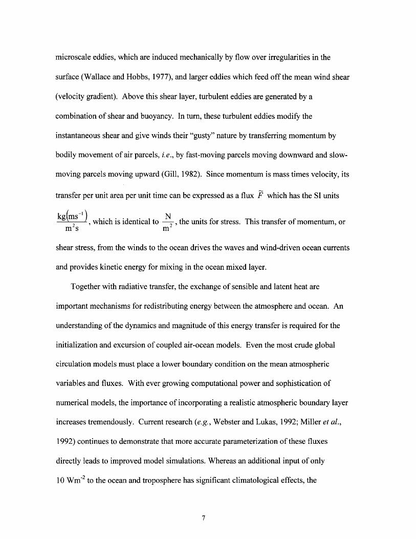
microscale eddies, which are induced mechanically by flow over irregularities in the

surface (Wallace and Hobbs, 1977), and larger eddies which feed off the mean wind shear

(velocity gradient). Above this shear layer, turbulent eddies are generated by a

combination of shear and buoyancy. In turn, these turbulent eddies modify the

instantaneous shear and give winds their "gusty" nature by transferring momentum by

bodily movement of air parcels, i.e., by fast-moving parcels moving downward and slow-

moving parcels moving upward (Gill, 1982). Since momentum is mass times velocity, its

transfer per unit area per unit time can be expressed as a flux F which has the SI units

kg(ms') N, which is identical to N , the units for stress. This transfer of momentum, or

mss m

shear stress, from the winds to the ocean drives the waves and wind-driven ocean currents

and provides kinetic energy for mixing in the ocean mixed layer.

Together with radiative transfer, the exchange of sensible and latent heat are

important mechanisms for redistributing energy between the atmosphere and ocean. An

understanding of the dynamics and magnitude of this energy transfer is required for the

initialization and excursion of coupled air-ocean models. Even the most crude global

circulation models must place a lower boundary condition on the mean atmospheric

variables and fluxes. With ever growing computational power and sophistication of

numerical models, the importance of incorporating a realistic atmospheric boundary layer

increases tremendously. Current research (e.g., Webster and Lukas, 1992; Miller et al.,

1992) continues to demonstrate that more accurate parameterization of these fluxes

directly leads to improved model simulations. Whereas an additional input of only

10 Wm-2 to the ocean and troposphere has significant climatological effects, the

uncertainty in current estimates of the surface heat budget exceeds this value, with

discrepancies as large as 80 Wm-2 in the warm pool region of the western Pacific Ocean

(Bradley et al., 1991). Decreasing this uncertainty and providing improved estimates of

the heat budget will result in increased performance in numerical models and improve our

ability to diagnose and predict climate and climate variability.

The research presented in this thesis is an investigation of the influence of wave-

induced processes on momentum exchange. The thesis explores modifications to

traditional flux parameterizations to account for sea state. This is accomplished by

investigating two separate approaches to incorporate sea state dependence into the

roughness length determination in the bulk aerodynamic method and a new approach to

incorporate wave-induced effects in the dimensionless dissipation rate in the inertial

dissipation method. Both investigations rely on comparison of the parameterized fluxes

with direct covariance fluxes.

Details of the experiment, instrumentation, and data processing are described in

Chapter 2. Chapters 3 and 4 provide the theoretical framework upon which this

investigation is based. A detailed derivation of the turbulent kinetic energy budget is

presented in Chapter 3, and a summary of the four standard techniques for estimating the

momentum flux, including an introduction to the well-accepted Monin-Obukhov

similarity theory, is provided in Chapter 4. Alternate parameterizations for both the bulk

aerodynamic and inertial dissipation methods are presented in Chapter 5, and their

performance is evaluated. The final chapter summarizes the findings of this thesis and

suggests areas of future research.

2. EXPERIMENT

2.1. DEPLOYMENT AND SITE SELECTION

The data used in this investigation were collected during the Coastal Mixing and

Optics (CMO) experiment, an Accelerated Research Initiative supported by the Office of

Naval Research (Williams, 1997; Galbraith et al., 1997). Four moorings were deployed

from August 1996 to June 1997 in the Middle Atlantic Bight, 90 km south of Martha's

Vineyard at approximately 40.5°N, 70.50E, as depicted in Figure 2.1. The four moorings

included a central mooring on the 70 m isobath, an inshore mooring located

approximately 10 km inshore along the 60 m isobath, an offshore mooring located 10 km

offshore along the 80 m isobath, and an alongshore mooring located 25 km east of the

central buoy along the 70 m isobath. The region has fine sediment and a smooth bottom

that slopes gently towards the shelf break 40 km to the south. The large-scale surface

heating and buoyancy advection at this site create a strong thermocline/pycnocline during

the late-spring and summer months. The extensive deployment was chosen so that the

observation period included the destruction of thermal stratification of the water column

in the fall and the subsequent redevelopment of stratification in the spring. In addition to

recording the seasonal evolution of stratification, the passage of numerous frontal systems

as well as the transits of Hurricanes Edouard and Hortense were observed. Due to the

variety of weather phenomena experienced at the site during the eleven-month

deployment, this data set represents a wide range of conditions and is unequaled in

previous investigations of mixing processes in coastal/shelf waters.

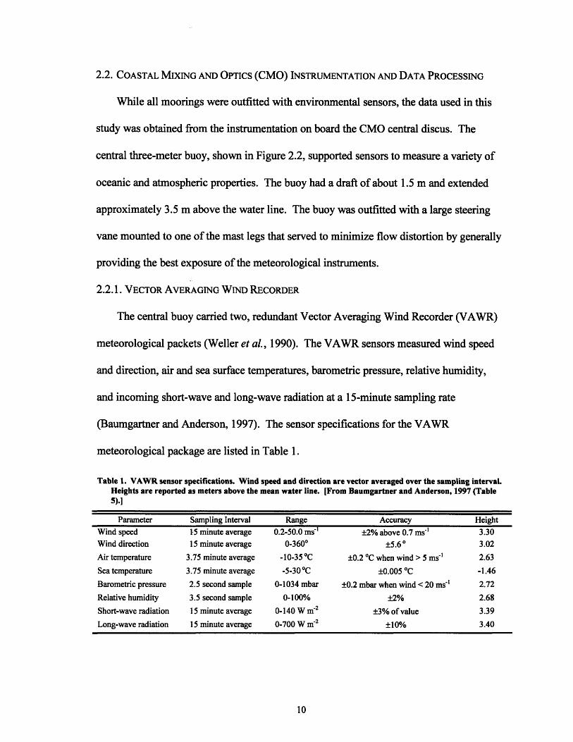
2.2. COASTAL MIXIN G AND OPTICS (CMO) INSTRUMENTATION AND DATA PROCESSING

While all moorings were outfitted with environmental sensors, the data used in this

study was obtained from the instrumentation on board the CMO central discus. The

central three-meter buoy, shown in Figure 2.2, supported sensors to measure a variety of

oceanic and atmospheric properties. The buoy had a draft of about 1.5 m and extended

approximately 3.5 m above the water line. The buoy was outfitted with a large steering

vane mounted to one of the mast legs that served to minimize flow distortion by generally

providing the best exposure of the meteorological instruments.

2.2.1. VECTOR AVERAGING WIND RECORDER

The central buoy carried two, redundant Vector Averaging Wind Recorder (VAWR)

meteorological packets (Weller et al., 1990). The VAWR sensors measured wind speed

and direction, air and sea surface temperatures, barometric pressure, relative humidity,

and incoming short-wave and long-wave radiation at a 15-minute sampling rate

(Baumgartner and Anderson, 1997). The sensor specifications for the VAWR

meteorological package are listed in Table 1.

Table 1. VAWR sensor specifications. Wind speed and direction are vector averaged over the sampling interval.Heights are reported as meters above the mean water line. [From Baumgartner and Anderson, 1997 (Table5).]

Parameter Sampling Interval Range Accuracy HeightWind speed 15 minute average 0.2-50.0 ms' ±2% above 0.7 ms- 3.30Wind direction 15 minute average 0-3600 ±5.6 o 3.02

Air temperature 3.75 minute average -10-35 OC ±0.2 OC when wind > 5 ms-' 2.63

Sea temperature 3.75 minute average -5-30 OC ±0.005 oC -1.46

Barometric pressure 2.5 second sample 0-1034 mbar ±0.2 mbar when wind < 20 ms' 2.72Relative humidity 3.5 second sample 0-100% ±2% 2.68

Short-wave radiation 15 minute average 0-140 W m-2 ±3% of value 3.39

Long-wave radiation 15 minute average 0-700 W m-2 ±10% 3.40

Figure 2.1. Coastal Mixing and Optics Site. [FromStenner, 1996.]

Figure 2.2. Coastal Mixing and Optics central 3 m

discus buoy. [From Baumgartner and Anderson,1997 (Figure 4).]

12

2.2.2. SoNIC ANEMOMETER

The central buoy also held a sonic anemometer which measured the longitudinal,

lateral and vertical wind velocities as well as the speed of sound. The sonic was mounted

between the VAWR wind sensors at a height 3.3 m above the sea surface and was

configured to burst sample twice per hour for a duration of 15 minutes.

Manufactured by Gill Instruments Ltd., the sonic consists of a sensing head and three

ultrasonic transducer pairs supported by three struts. The struts are placed asymmetrically

to provide ± 120' of open exposure. The sonic anemometer is specified to operate with

1.5% accuracy for wind speeds between 0-60 ms-1 (Yelland et al., 1994). Each pair of

transducers alternately transmits and receives pulses of high frequency sound waves. All

three axes complete these firings every 6 ms, which represents a sampling rate of 168 Hz.

Using overlap section averaging, every eight complete transit time evaluations are

averaged to produce the 21 Hz output. The transit time data were transformed into an

orthogonal coordinate system by which the speed of sound and wind velocity were

calculated by determining the times of flight, t, and t2, between any pair of transducers.

Specifying V as the air flow parallel to the line of the transducer pair, the flight times are

defined by

1 1ti = and t2 - (2.1)

c+V c-V

where 1 is the distance between the transducers (0.15 m) and c is the speed of sound in air.

The wind velocity and the speed of sound can be determined explicitly:

V = (I t21) (2.2)2 ti t2

c = - -+ - (2.3)2 ti t2

Once the speed of sound c is determined, the virtual temperature T, expressed in

Kelvin can be calculated by

C2 UN

T, 403 (2.4)403

where both c and uN are given in ms1 , and the term

2 2 2 (2.5)

corrects for the curvature in the path that the sound waves travel due to air flow

perpendicular to the line of the transducers (Fairall et al., 1997).

2.2.3. WAVE HEIGHT MEASUREMENTS

The surface wave data were measured by a SeaTex Waverider buoy (Barstow et al.,

1991). The Waverider buoy was configured to burst sample once per hour at a 1 Hz

sampling rate for a duration of approximately 17 minutes and measured motion, spectral

data, and scalar wavefield parameters, including significant wave height and primary

wave period T (Galbraith et al., 1997). The wave dispersion equation relates the radian

2nt 2ntfrequency, o - -, and wave number, k =- , to the water depth, D:

T '

0C2 = gk tanh(kD) (2.6)

where X is the wavelength and g is the acceleration due to gravity (Earle and Bishop,

1984). Since a wave travels a distance of one wavelength in one wave period, the phase

speed can be defined as

C tanh(kD) (2.7)T k

Thus, with knowledge of only the water depth and the wave period, the radian frequency,

wave number, and phase speed can be determined in an iterative fashion.

2.3. MARINE BOUNDARY LAYER EXPERIMENT

This investigation also relies on data analyzed as part of the ONR's Marine Boundary

Layers (MBL) Accelerated Research Initiative (Edson et al., 1997). This program was

designed to examine the 3-D structure of the marine boundary layers. The open ocean

component of the MBL program was conducted off Monterey, California, in April and

May of 1995 and involved the R/P FLIP, the NOAA/Oak Ridge LongEZ aircraft, and

three research vessels. The emphasis of this program was on improving the

understanding of flux profile relationships over the open ocean. During the field

experiment, investigators deployed a 18 m mast at the end of FLIP's port booms, setting

up a vertical array of 12 levels of cup/vane anemometers to provide mean profiles. Four

levels of sonic anemometer/thermometers and three levels of static pressure sensors were

also deployed from this mast in order to examine the flux and dissipation rate profiles and

provide the necessary scaling parameters to compute the dimensionless profile functions.

A single wave-wire was deployed directly beneath the mast to measure the instantaneous

wave height, which was nominally 3 m beneath the lowest cup anemometer.

3. THEORY

3.1. BASIC EQUATIONS

Using the results obtained by Shaw (1990), the Navier-Stokes equations in a rotating

Eulerian reference frame are

a a apu, +- PUuk P i6,k k Pg 3 - 2pnS kljUk (3.1)at xk k,

where

(Y u = au k 2, + u

S k ik ik = o ik + P (3.2)x &k i 3 x 1 8x

In this expression, T1 is the dynamic viscosity, Q is the angular velocity of the earth, 1

is a unit vector along the axis of rotation, aik defines the stress tensor, and is a second

molecular viscosity which applies to compressible flow. In general, the atmosphere

boundary layer may be treated as incompressible flow and the Boussinesq approximations

may be applied (Panofsky and Dutton, 1984). This reduces the continuity equation

dp 8+ pu =0 (3.3)at ax&

to

U = 0 (3.4)8xi

Applied to equation (3.1), these approximations yield

au au 1 p 2u,S+uk - + 2 krlj Uk 6 i3 ix8B+ (3.5)

w t x k P oxSi 1xk k

where v - i/p is the kinematic viscosity (Shaw, 1990).

The first law of thermodynamics applied to a fluid provides the general equation of

heat transfer

as 0s ,u, 0 OT ORkpT s+u =3 k -- + kO k (3.6)at - x x k x k cx k xk

Rk is the radiative flux; kc is the molecular conductivity; and s is entropy, for which

changes can be expressed in terms of the standard definitions of specific heat at constant

pressure c, and the equation of state

Tds = cdT- dp (3.7)

A common expression for the equation of state is

p = pRdT, (3.8)

where Rd is the gas constant for dry air and Tv is virtual temperature, a function of specific

humidity q.

Substituting from the equation of state, defining the potential temperature 0 as

0 - T(1000/p)R/cP where T is in Kelvin and the pressure is given in millibars, integrating

equation (3.7), and neglecting the term representing mechanical-to-thermal energy

conversion transforms equation (3.6) to

dO 0 8 0 kc 2T 1 O Rk=-+uk-- (3.9)

dt at Oxk Tpcp OxkO k PC T OXk

The equation for the conservation of specific humidity q may be similarly written as

dq _q Oq x 2q- + = - u = D (3.10)dt at x i ax jx pj

where Dq is the molecular diffusivity of water vapor.

3.2. EQUATIONS FOR TURBULENT MEAN FLOW

Equations (3.3), (3.5), (3.8), (3.9), and (3.10) form a closed set of seven equations

governing seven variables. However, the equations contain nonlinear terms which render

them impractical to describe turbulent flow. Instead, realizing turbulent flow as a

stochastic process and applying Reynolds decomposition, which expresses the variables

as a sum of a mean and fluctuating part [i.e., (x, y, z, t) = 4(x, y, z, t) + '(x, y, z, t) ],

transforms equation (3.5) to

u, au;f - u+ ,au - au au; I 1 0p'+"+ U +U? +U +u -

at at a ax ax ax p (3.11)x(3.11)

p' 1 .. (w, +u')+ - g_8i3 + V 2skrljuk - 2Sk rlj UkP 8ax,i x.x ,

Ensemble averaging (3.11) yields the balance for mean momentum in a turbulent

atmosphere:

au -au 1 aj a au auu'S+ u - + 2 2-S&k1j Uk - - - j (3.12)at ax &i &j xj &j

The last term on the left-hand side of (3.12) represents acceleration and the Coriolis

effect. The first term on the right-hand side is the pressure gradient force, and the second

term is the frictional force due to molecular viscosity. The last term represents the drag

resulting from momentum transfer by turbulence and is the kinematic form of the

divergence of the Reynolds stress tensor,

'r = -puu (3.13)

For boundary layer studies the most important terms of the Reynolds stress tensor

represent the vertical transport of horizontal momentum, defined as

= - vw'] (3.14)

Determining the means to best parameterize this flux is the main focus of this thesis and

will be discussed in detail in the following Chapter.

The same Reynolds decomposition and ensemble averaging procedure that were

applied to equation (3.5) can be applied to the potential temperature and water vapor

balances to yield

ao O auJ' 1 0 aRk- + u - (3.15)at Oxj 8x, cP T axk

and

L + u.=a - (3.16)at 'aix ax

3.3. EQUATIONS FOR TURBULENT KINETIC ENERGY

An expression for the time rate of change of the Reynolds stress tensor may be

formed by subtracting (3.12) from (3.11) and applying the hydrostatic and Boussinesq

approximations:

au: - u' ,u ua 1 ap' T: '2U du + u . u + uP ++ ' -+ gS+v + (3.17)at , x d x J ax dr T, aj x,.x 7

The relation for u' can be written

au au -- u ' u u' 1 ap' T aUp au au'at + u a + u, + U' u, + gSp3 + v + (3.18)at ax, qx, ax, ax, T, ax ax, ax,

Note that the Coriolis term is not included because scale analysis shows that turbulent

velocity fluctuations occur at time scales too short to be influenced by the Coriolis force

(Shaw, 1990). Multiplying (3.17) by u' and (3.18) by u, averaging both equations and

adding them yields the equation for the time rate of change of the Reynolds stress tensor

S- -auu , -- u ,, , 1 u'ap' u;ax'uu = -uj uu -u u x uuju + jt , ,o xi a0 u ' 2x &U (3.19)

T i ) + x i a x x xxi a

Using the notation in Shaw (1990), the mean kinetic energy of turbulence (TKE) per

unit volume is defined as

1E = 2 pu u: (3.20)

Alternately, meteorologists generally use the kinematic form to define the TKE

E IE -=- uiu, (3.21)

P 2

and the instantaneous net contribution to the TKE

1e' - 2 u,'u" (3.22)

The equation for rate of change of the turbulence kinetic energy follows directly from

(3.19) by setting p=i and making use of the continuity equation:

8£ - e u g u 'e' 1 au p' au" 9u't -u -u ' + u-T= ' 3 - v (3.23)

at xj , 8x, T , 3 I, 8xx Pxj

The first term of the right hand side of the equation represents the rate of change of

TKE due to advection. The second term represents the generation of mechanical

turbulence through shear, while the third term represents buoyancy production. The

fourth and fifth terms are transport terms which neither produce nor consume energy, but

act to redistribute TKE within the boundary layer; the first transport term represents the

divergence of turbulent kinetic energy flux, and the second is due to the divergence of

pressure-velocity covariance. The last term is always negative and represents the

dissipation 6 of turbulent kinetic energy at the smallest scales due to viscous forces.

The energy budget simplifies greatly under horizontally homogeneous conditions for

which mean quantities depend only on the vertical coordinate. Furthermore, since we

expect the smallest scales of motion to have an isotropic structure, the expression for

dissipation can also be simplified. Replacing ui and x, by (u,v,w) and (xy,z),

respectively, in equation (3.23), the TKE budget equation for stationary, horizontally

homogeneous conditions with zero subduction (iT = 0) becomes

Nw X+ g 1 aw'p' aw'e'- u v'w'- + -w'T' = 0 (3.24)

az az T, p az az

This is the form of the TKE budget that will be used in the following discussions.

4. METHODOLOGY

There are four standard methods for determining the momentum flux from

atmospheric information:

(i) direct covariance (eddy correlation);

(ii) mean profiles;

(iii) bulk aerodynamic; and,

(iv) direct / inertial dissipation.

4.1. DIRECT TECHNIQUES TO DETERMINE THE MOMENTUM FLUX

4.1.1. DIRECT COVARIANCE (EDDY CORRELATION) METHOD

The direct covariance method is the standard upon which all other methods of

estimating the momentum flux are based. Whereas the other three methods rely on

similarity theory, the covariance method is a direct computation of the Reynolds stress

and yields an unbiased estimate of the flux (Fairall et al., 1990). Revisiting equation

(3.14), the wind stress can be determined directly by measuring the turbulent components

of the streamwise and vertical wind velocity:

S= -pI'w' + '] (4.1)

In practice, the ensemble average is approximated by averaging simultaneous

measurements of the turbulent components of wind velocity and cross correlating them

over a finite time interval (Frederickson et al., 1997). The assumption that allows us to

relate time averaged fluxes to ensemble averaged fluxes is referred to as ergodicity

(Panofsky and Dutton, 1984). For stationary conditions, as the length of the averaging

interval increases, the accuracy of this approximation generally increases, although there

is a tradeoff between the choice of averaging period and nonstationarity of the data

(Mahrt et al., 1996).

The primary disadvantage of the direct covariance method is that comparative studies

(e.g., Fairall et al., 1990; Edson et al., 1991; Edson and Fairall, 1998) indicate that the

direct covariance method is highly susceptible to flow distortion. Additionally, unless the

measurements are made from a stable platform, such as a fixed mast or tower, the data

must be corrected for platform motion contamination. Clearly, this limits the

applicability of this method from ships and buoys.

4.1.2. MOTION-CORRECTED COVARIANCE METHOD

However, a great deal of effort has been made in recent years to compute direct

covariance fluxes from moving platforms to improve flux parameterizations over the

open ocean (e.g., Fujitani, 1981, 1985; Tsukamoto, 1990; Dugan et al., 1991; Anctil

et al., 1994; Fairall et al., 1997; Edson et al., 1998). If one wishes to apply the direct

covariance method on a moving platform, then the orientation and motion of the platform

must be accounted for before computing the correlations (Fairall et al., 1990). Surface-

following buoys experience a variety of motions including instantaneous tilt of the

sensors due to platform movement, angular velocities about the platform's local

coordinate system, and translational velocities with respect to a fixed frame of reference

(Fujitani, 1981; Hare et al., 1992). In vector notation, the motion corrected wind speed

Vr ue can be written as

true = T(obs b XR)+ Vmo t(4.2)

where T is the rotation matrix which transforms measurements taken in the buoy

reference frame to earth coordinates; Vobs and Ob are the measured wind speeds and

angular rates in the buoy frame of reference, respectively; i is the position vector of the

wind sensor with respect to the motion package; and, Vmo, represents the translational

velocities in the fixed frame (Anctil et al., 1994; Edson et al., 1998). The product

2b x TR represents the angular velocity in the fixed frame.

Removal of this motion from our wind sensors requires us to measure the three

dimensional translational motion of a reference point on the buoy, the three angular

rotations about that point, and the Euler angles required for the transformation matrix.

During the CMO experiment, three Systron Donner quartz sensors recorded the pitch,

roll, and yaw rates (d, 6, and 1, respectively), and a three-axis Columbia linear servo

accelerometer provided the linear accelerations of the buoy ( , j , and 2, respectively) .

All of the sensors were strapped down in the hull of the discus buoy. One of the main

advantages of a strap-down system is that it readily computes the angular rates in the

buoy frame of reference:

2b =XP+j+ (4.3)

where i , J, and k represent the unit vectors in a right-hand coordinate system pointing

from the buoy fin to front, starboard to port, and vertically up, respectively.

The three Euler angles which specify the rotation of the buoy are the pitch , roll ,

and yaw . Using the approach described by Edson et al. (1998), the Euler angles are

approximated using complimentary filtering, which combines the high-passed filtered

integrated angular rates with the low-passed linear accelerations as

D 1 j) s+ (44)t+lg rs+l

1 x rsOe I - + - (4.5)

'r+lg Ts+l

and

1 1sSsliow + TS (4.6)

t +1 ts +1

where s represents the differentiation operator such that I) = sio, r is a time constant,

Ys ow represents the compass output, and a small angle approximation is made in (4.4)

and (4.5).

Given the Eulerian angles, the rotation matrix T which transforms measurements

taken in the buoy reference frame to earth coordinates can be expressed:

cosY cosO- sin cos + cosYsin sin Q sin sin + cosY sinOcos DT= sin cosO cosY cos D + sin Y sin O sin D sin O cos D sin I - sin ) cosPY (4.7)

L - sin cos o sin Q cos E cos 0

Again, the sign convention corresponds to a right-handed coordinate system with Y

positive for the ship's bow yawed counter-clockwise from north, D positive for the port

side rolled up, and 0 positive for the bow pitched down (Edson et al., 1998).

The accelerations are then rotated into the vertical using the rotation matrix T before

adding the gravity vector, k = (0,0,-g), to the rotated accelerations. The resulting

accelerations are then high-pass filtered to remove any drift before integrating. This

process can be expressed as:

V(t)mot = t [Hp(T (t) + t (4.8)

where Hp represents a high-pass filter operator. The strapped-down system thereby

provides all the terms required by (4.2) to compute the true wind velocity. These

corrected velocities are then used to compute the wind stress.

4.2. INDIRECT TECHNIQUES TO DETERMINE THE MOMENTUM FLUX

Monin and Obukhov (1954) postulated that the turbulent fluxes of atmospheric

momentum and heat energy in a stationary, horizontally homogeneous surface layer is

determined by the height above the surface z, the buoyancy parameter g/--, the friction

velocity u., and the surface buoyancy flux w'O, 0 where 0, is the virtual potential

temperature and accounts for density changes due to humidity fluctuations and g is the

acceleration of gravity (Lumley and Panofsky, 1963; Wyngaard, 1973). The friction

velocity u. is defined in the manner of equation (4.1) from the surface stress:

u, = = [(-u,w,)2 + (_ ,w,)2 (4.9)

Largely on the basis of dimensional arguments, Monin-Obukhov (MO) similarity

theory predicts that the various terms in the TKE budget [equation (3.24)] are universal

functions of the MO stability parameter after normalization by the appropriate scaling

KZparameter, -K3

U,

EIC3 = = t p 0)- Ote 0(4.10)

where K is the dimensionless von Kirmn constant, generally assumed to be 0.4

(H6gstr6m, 1987; Edson et al., 1991; Fairall et al., 1996a); 4, is the dimensionless

dissipation function; , and ,, are the dimensionless transport terms; and, ,m is the

dimensionless shear defined as

4M () _Z + (4.11)

The stability parameter represents the ratio of the height above the surface z to the

Monin-Obukhov length L defined as L -, such that -. In unstablegrc wOv 0 L

conditions the Monin-Obukhov length represents the height where mechanical and

buoyant production of turbulence are approximately equal, i.e., at this height, = -1. At

heights below this level, shear production dominates; while above this level, buoyancy

dominates. In stable conditions the stratification consumes some of the kinetic energy

such that 4 represents the ratio of buoyant consumption to shear production.

4.2.1. MEAN PROFILE METHOD

Generally, the wind direction is assumed to be constant in the surface layer such that

the coordinate system is rotated so that V = 0. In this coordinate system the wind shear

becomes

a= u, () (4.12)az rz

Upon integrating the above equation, one obtains the logarithmic wind profile for neutral

conditions upon which the profile method is based:

(z)= u-(zo)+* In z- -WM (4.13)K zo L

where zo is the aerodynamic roughness length and reflects the roughness of the surface,

and y,M is the integrated form of , M. Using equation (4.13), it is relatively easy to

obtain u. and zo from a given wind profile: plotting u as a function of ln(z) - Y ()

results in a straight line with u as the slope and u* ln(zo) as the intercept.K K

Therefore, the implementation of the profile method requires the deployment of

multiple sensors at varying heights. This type of deployment in the marine surface layer

creates a number of problems. In addition to the cost associated with employing an array

of sensors, excellent relative calibration among sensors is required due to the small shear

found over the ocean. Additionally, calibration drift between the individual sensors due

to mechanical degradation may result in large uncertainties among measurements.

Another physical limitation of the profile method is the requirement for the lowest sensor

to be at least two or three wave heights above the interface since the presence of

undulating long waves causes deviations to the logarithmic profile (Geernaert, 1990).

This requirement further limits the placement of the sensors since they upper height is

already bounded by the height of the surface layer, the region within which the fluxes

vary by no more than 10% of their surface values, a requirement of MO similarity theory.

Finally, and probably most importantly, the physical set-up of the array renders the

sensors extremely sensitive to flow distortion and motion contamination. Therefore, this

method has rarely been implemented over the ocean.

4.2.2. BULK AERODYNAMIC METHOD

The bulk method is the simplest and most widely used of the four techniques. The

bulk method is an application of the profile method for which the structure of the

atmospheric boundary layer is estimated by using measurements at one level and

assuming a logarithmic wind profile. The standard bulk expression for the stress

components is

To = pu* 2 = PaCD(i(Z)-U( (Z)i z)- (Z) (4.14)

where CD is the bulk transfer coefficient for stress; u, (z) is the average of one of the

horizontal wind components relative to the fixed Earth measured at some reference height

z; and u, (zo) is the surface current (Fairall et al., 1996a). The velocity difference is,

therefore, the velocity relative to the ocean surface.

Equation (4.14) can then be used to define the drag coefficient as

K

CD (z) = log(z/z (4.15)

The neutral drag coefficient is related to the roughness length by

CD,(z) = [log(z (4.16)

such that

(CDN)' Co

(C+ = CD (4.17)1+

where the subscript N denotes the value in neutral conditions; and, IJM (g) is the MO

similarity profile function. The following expressions of Businger et al. (1971) and Dyer

(1974) are the most commonly used:

WM ()=(1-16) Y <0 (4.18a)

WM ( I)= (1 + 5) 2 0 (4.18b)

Using the approach described by Smith (1988), the velocity aerodynamic roughness

length zo can be expressed as

zo = zS + Zr (4.19)

where z, and zr represent the aerodynamic roughness of smooth and rough flows,

respectively. The roughness length for a smooth surface depends on the viscosity of air

v and the friction velocity (Businger, 1973):

Vz, 9u (4.20)

9u,

The determination of zr is based on the relationship proposed by Charnock (1955).

Using dimensional analysis, Charnock assumed that the aerodynamic roughness length of

the surface for well-developed seas is proportional to the wind stress which generates and

supports the surface waves and gravity which acts as the restoring force:

2

zr au (4.21)

where a c is the Charnock "constant" for which values between 0.010 and 0.035 can be

found in the literature (Garratt, 1992). Representing the ratio of inertial force to

gravitational force, the Charnock constant is analogous to a Froude number.

The method and algorithm for computing the bulk estimates are described in detail in

Fairall et al. (1996a). In summary, the bulk estimates are calculated by using the

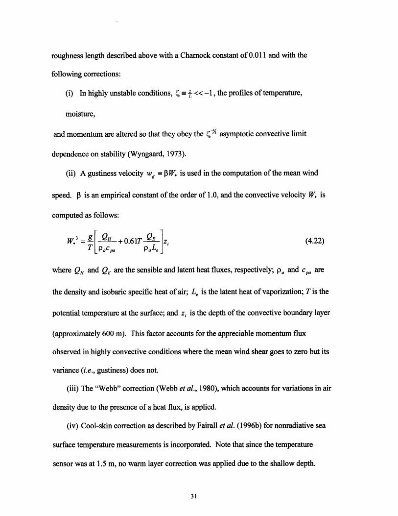
roughness length described above with a Charnock constant of 0.011 and with the

following corrections:

(i) In highly unstable conditions, << -1, the profiles of temperature,

moisture,

and momentum are altered so that they obey the 4 - asymptotic convective limit

dependence on stability (Wyngaard, 1973).

(ii) A gustiness velocity w, - P W is used in the computation of the mean wind

speed. P is an empirical constant of the order of 1.0, and the convective velocity W is

computed as follows:

W. T = [ Pc + 0.61T pE z, (4.22)T pacp PaLe

where QH and QE are the sensible and latent heat fluxes, respectively; pa and c, are

the density and isobaric specific heat of air; Le is the latent heat of vaporization; T is the

potential temperature at the surface; and z, is the depth of the convective boundary layer

(approximately 600 m). This factor accounts for the appreciable momentum flux

observed in highly convective conditions where the mean wind shear goes to zero but its

variance (i.e., gustiness) does not.

(iii) The "Webb" correction (Webb et al., 1980), which accounts for variations in air

density due to the presence of a heat flux, is applied.

(iv) Cool-skin correction as described by Fairall et al. (1996b) for nonradiative sea

surface temperature measurements is incorporated. Note that since the temperature

sensor was at 1.5 m, no warm layer correction was applied due to the shallow depth.

One potential source of error in the bulk aerodynamic method is in the

characterization of the roughness length by equations (4.19) through (4.21). Charnock's

expression for the roughness of the sea surface has been shown to be generally valid for

moderate to high wind speeds at unlimited fetch and duration (Geernaert et al., 1986).

However, upon examining equation (4.21), one sees that no characteristics of the wave

field are truly present. This implicitly assumes that the wind and wave fields are in local

equilibrium; consequently, Charnock's relation will only give consistent results for a

fully-developed sea (Donelan, 1990; Maat et al., 1991; Dobson et al., 1994). Sudden

changes in the wind, such as that due to frontal passages, result in the wind field being

temporarily out of equilibrium with the existing wave field (Smith, 1988). The

momentum transfer between the wind and wave fields as the waves grow or decay in

response to the forcing is not considered in Charnock's expression. Additionally, the

influence of varying fetch and possible interactions with the bottom in shallow water are

not included. The neglect of these processes probably explains the wide range of values

for the Charnock's "constant" found from different experiments. Finally, implementation

of the bulk aerodynamic method using buoy data often places the measurements where

the waves cause changes to the log profile. All of these effects result in changes to the

drag coefficient which are sea-state dependent.

4.2.3. DIRECT AND INERTIAL DISSIPATION METHODS

The direct dissipation and the inertial dissipation methods differ only in the manner

in which the dissipation rate for turbulent kinetic energy is computed. Direct

measurements of dissipation rates are determined by integrating over the spectrum of the

velocity derivatives (Fairall and Larsen, 1986):

E = 1i5v- a 1vC2 (4.23)

Since the fluctuations have a spatial resolution that approaches the Kolmogorov

microscale (typically 1 mm in atmospheric flows), hot-wire anemometers must be used to

obtain direct measurements (Edson and Fairall, 1998). While this method has been used

overland, its applicability over the ocean is limited due to contamination and even

destruction of the wires by sea spray (Edson and Fairall, 1998). Therefore, the direct

dissipation method is rarely employed over the ocean.

Instead, the inertial subrange method, which requires frequency responses only up to

the order of 10-100 Hz, is more commonly employed (Smith et al., 1996; Fairall et al.,

1997). In the inertial subrange of local isotropic turbulence, the one-dimensional velocity

variance spectrum (D, can be expressed as a function of wavenumber magnitude as

Du (k) = a.e y k (4.24)

where a, is the one-dimensional Kolmogorov constant, taken to be 0.52 (H6gstr6m,

1996), and k is the wavenumber.

2nf coInvoking Taylor's frozen turbulence hypothesis, k - = , the velocityU, Us

variance spectra can be related to the frequency spectra S, as

kS. (f) (k) =, (4.25)(T.. Xe,,. Xatt, + att2 ) = u )

wherefis frequency, S, is the spectrum of the streamwise velocity U, as a function of

the angular frequency o, and T,, and (att, + att2 ) are correction factors:

(i) T,, is a correction for inaccuracies in using Taylor's hypothesis to estimate the

magnitude of wavenumber spectra in the inertial subrange and has the form given by

Wyngaard and Clifford (1977):

T,, = 1 _) + 2- C ,) (4.26)9 U 2 3 Us2

where au2 , a, v, a 2 are variances (uu, vv and ww) computed from the same time series

that produced the spectral estimate (Hill, 1996).

(ii) The terms att, and att2 correct for excess damping of higher frequencies caused

by the eight-fold pulse-averaging of the sonic anemometer (Henjes et al., 1998) and has

the forms

sin 2 (

att = (4.27a)

7fo)

y_ sin2 ( f)] sin2[ l(fo-f)

att2 0 (4.27b)f0 - I n (f _ f - 7) 2 - 2

S fo , U,

where fo is the Nyquist frequency, 20.833 Hz.

Note that spatial averaging also reduces the spectral estimates at high frequencies, in

the manner described by Kaimal et al. (1968):

sin2 klQ = 2 (4.28)

kl

where 1 is the separation distance between the sonic heads. However, the effect of line-

averaging is negligible for k < 1. Since we have limited the frequency range such that

U-f < this correction is not needed.

2nl

When using the inertial dissipation method, it is generally assumed that the transport

terms cancel (Hicks and Dyer, 1972; Large and Pond, 1981; Dyer and Hicks, 1982; Large

and Businger, 1988) so that a balance exists between the viscous dissipation and

production (buoyant and shear) of TKE. Under this assumption, equation (4.10) reduces

to

3 = (W + M ()- (4.29)

A potential source of error in using the inertial dissipation technique arises from the

assumption that there is a balance between TKE production and dissipation. Recent

investigations (Vogel and Frenzen, 1992; Frenzen and Vogel, 1992; Thiermann and

Grassl, 1992; Yelland and Taylor, 1996; Edson et al., 1997; Edson and Fairall, 1998)

suggest that there is a local imbalance between the pressure and energy transport terms

such that the magnitude of the energy transport term +, ( ) is greater than the magnitude

of the pressure transport term +,, (c), and TKE production exceeds dissipation by 15-

20%. Over the ocean, it has been hypothesized by Edson et al. (1997) that this

dissipation deficit is due to the flux of energy going into ocean waves.

The flux of kinetic energy, F(z), into a layer of air over a horizontally homogeneous

surface is given by

F(z) = u'w'u(z) + v'w'v(z) + w'e' + -w'p' (4.30)p

where the first two terms on the right-hand side of the equation represent the flux of mean

flow kinetic energy and the last two terms represent the rate of diffusion of kinetic energy

(Edson et al., 1997). Over land, it is generally assumed that there is no energy flux

through the ground so that the flux entering the layer at height h can be related to the total

rate of dissipation within the layer by

h h

fdz = -F(h) + T w' T'dz (4.31)0 v0

where the last term represents the generation of kinetic energy due to buoyancy flux

(Edson et al., 1997). For neutral conditions, equation (4.31) states that the flux of kinetic

energy into the layer equals the dissipation within that layer; i.e., production balances

dissipation. However, over the ocean, where the exchange of momentum from the

atmosphere to the ocean results in wind-driven waves and currents, the surface energy

flux F(O) is not negligible and the additional forcing mechanism of the surface waves

must be included.

The effects of surface waves are included in the KE energy budget equation (3.24)

and energy flux equation (4.30) by decomposing the velocity into mean, turbulent, and

wave-induced components

u(t) = i + u'(t) + i(t) (4.32)

where the tilde represents the wave-induced component. The wave-induced component is

defined with the use of the phase-averaging operator as described by Finnegan et al.

(1984):

(u(t)), = + (t) = lim [ N u(t + no) (4.33)NL-oI NLL n=1

(t) = (u(t)), - U (4.34)

where to is the period of the organized oscillation and NL represents the number of

consecutive wavelengths averaged together to get one phase-averaged wave. This type of

averaging can be used to rewrite equation (3.24) to include the wave-induced

contributions. An approximation of the steady state solution of the TKE energy budget is

S- + pIz 8z T az 0z

(4.35)- c +w'e' +- U.] " + 4.5=0az az 2 axx &x

where r and - can be viewed as the wavelike fluctuations in the background Reynolds

stress due to the presence of waves

= (uu; -'u u (4.36)

such that the sum of the last two terms in brackets represents the interaction between the

wave field and the wavelike part of the turbulent stresses and constitutes a loss of kinetic

energy (Finnigan et al., 1984). In this form, the shear production P now includes terms

representing the wave-induced momentum flux,

U W VW (4.37)P = -u-w' + =-]- [v'w' +vw (4.37)az az

The production of kinetic energy is therefore the result of a forcing mechanism that is a

function of sea state.

Similarly, the transport of energy from wind to waves at the ocean surface is actually

the lower boundary condition of the pressure transport term, i.e.,

F(1) -wp o 0t Po (4.38)p p at

where X is the surface elevation and the time rate of change is known as the piston

velocity. This term must be included in equation (4.31) in over ocean studies such that

h h

Jcdz = F(O)- F(h) + w'T,' + t~ z (4.39)0 TV

where the fluxes now represents both turbulent and wave-induced fluctuations. Unlike

the solid boundary for which the flux through its surface is negligible, there is a transfer

of energy from the atmosphere to the ocean, and the total amount of dissipation within the

wave boundary layer is expected to be less than required to balance the energy flux into

the layer; a phenomenon supported by recent investigations (Yelland and Taylor, 1996;

Edson et al., 1997; Edson and Fairall, 1998). Thus, in the wave boundary layer, the

transport of energy and momentum to the ocean from the atmosphere is not adequately

described using Monin-Obukhov similarity theory, and additional scaling parameters are

required for similarity.

5. ANALYSIS AND RESULTS

The objective of this analysis is to improve estimates of the momentum flux using

modified forms of the bulk aerodynamic and inertial dissipation methods. The

modifications to the bulk aerodynamic method involve the derivation of a roughness

length parameterization which is sensitive to sea state. These modifications are drawn

from comparisons with direct covariance and inertial dissipation flux estimates. In the

case of the inertial dissipation momentum fluxes, additional parameterizations are applied

to account for the effects of surface waves and the non-zero energy flux from the

atmosphere to the ocean.

5.1. DATA SELECTION

The data sets obtained from both the VAWR sensor and sonic anemometer span the

entire eleven months from August 1996 to June 1997 and represent a total of 15,262 data

points (2 measurements per hour for approximately 318 days). Of these measurements a

total of 2,303 points, or 15%, were removed prior to processing for one or more of the

following reasons:

(i) Instrument failure (VAWR and/or sonic anemometer).

(ii) The velocity spectrum for inertial dissipation calculations did not meet the -

slope criteria [see equation (4.24)] and did not allow the calculation of dissipation

estimates. Possible reasons include rain and spray contamination and obstructions to the

path (e.g., due to a seagull sitting on the sensor).

(iii) Flow distortion, which arises when the relative wind direction is greater than

+ 600 from head on.

The wave height data set represents 241 days of the eleven-month deployment, but

only 1 measurement per hour was taken for a total of 5,778 points. In order to insure that

oceanographic conditions resulted from locally-generated seas and not from swell

propagating into the test site, 8% of the wave data were discarded prior to processing

because two distinct peaks were present.

For motion-corrected covariance calculations, the data set was further limited by the

amount of data collected by the motion-correction package. This package collected 30

minutes of 10 Hz data at noon and midnight for 317 days which produced a data set

totaling 634 direct covariance flux estimates.

5.2. TRADITIONAL APPROACH

Using the procedures outlined in Chapter 4, the friction velocity u., as defined by

equation (4.9), was calculated using the bulk aerodynamic, inertial dissipation, and direct

covariance methods. Figures 5.1 through 5.3 are comparisons of the u. calculations. The

inertial dissipation and bulk aerodynamic methods provide remarkably similar values for

u, < 0.6 m/s (Figure 5.1). At higher wind speeds, the inertial dissipation method predicts

progressively higher values of u,. than the bulk aerodynamic method, although the values

generally exhibit less than a 12% difference. Compared to friction velocity values

computed by the motion-corrected covariance method (Figures 5.2 and 5.3), both the bulk

aerodynamic and inertial dissipation methods provide u. estimates which are consistently

7-12% lower than expected for u. > 0.2 m/s. This would suggest that although the two

methods provide quite similar results, these values are underestimating the actual

momentum flux over the ocean.

Friction Velocity u. Comparison0.9

0.8 -

0.7

E

0 0.5

oo 0.4

m 0.3-

0.2

0.1 - -

0 I I

0 0.1 0.2 0.3 0.4 0.5 0.6 0.7 0.8 0.9Inertial Dissipation u, (m/s)

Figure 5.1 A comparison of the friction velocities, u., estimated using the bulkaerodynamic versus inertial dissipation methods and bin-averaged in increments of0.02 m/s. The error bars denote the standard error (standard deviation divided by thenumber of points).

Original Bulk Aerodynamic Friction Velocity u. Comparison

0.9

0.8

0.7E

=0.6

E 0.5C>0.4

a0.3

5 0.2

0.1

0.2 0.4 0.6Direct Covariance u. (m/s)

0.9

0.8

S0.7+

0.6 +0.2

E o.5 -1±c ++

o ++ID0.43D0.3 +

m5 0.2

0.1

00 0.2 0.4 0.6

Direct Covariance u. (m/s)

0.8

0.8

Figure 5.2 Friction velocity, u., comparisons of the bulk aerodynamic versus motion-

corrected covariance method. Values of u,. are bin-averaged in increments of

0.02 m/s.

Original Inertial Dissipation Friction Velocity u. Comparison

0.9

0.8

0.7E

S0.6C

0.5 .. .

0. 3 . .. ..- : •.•a 0.2C() ..

0.1 .

00 0.2 0.4 0.6

Direct Covariance u. (m/s)

0.9

0.8x

- 0.7E" 0.6 x

o0.5 X

0.3 x

( 0.2 /xx x

x x

0.1 X

00 0.2 0.4 0.6

Direct Covariance u. (m/s)

0.8

0.8

Figure 5.3 Friction velocity, u., comparisons of the inertial dissipation versus motion-

corrected covariance method. Values of u. are bin-averaged in increments of

0.02 m/s.

The neutral drag coefficient CDN described by equation (4.17), was calculated by the

bulk aerodynamic, inertial dissipation, and direct covariance methods for the following

four wave-age bins:

C,(i) 1 _ 2 4 ;

U,

C(ii) 24 < C 28;

C(iii) 28 < C <_ 32; and,

C(iv) 32 < C;

U,

where C, is the phase speed of the dominant seas, calculated using equation (2.7). The

first wave-age bin corresponds to young (developing) seas, the second and third wave-age

bins represent seas for which the waves receive no additional energy input from the wind

and are considered fully-developed, and the last wave-age bin corresponds to waves that

Care decaying. [An alternate expression for the wave age is l , where young waves

UION

Ccorrespond to 0.22 < < 0.29 and fully-developed waves are represented by

UI0N

C0.5 < U < 1.25 (Donelan, 1990).] Interestingly, less than 10% of the data represent

U10N

conditions in which the seas were growing. The absence of young waves from the data

set most likely indicates a limit in the techniques used to detect young waves. A review

of the meteorological record reveals that the CMO test site experienced numerous frontal

passages and storm systems (including two tropical storms) with wind conditions that

should be associated with new wave development. One limitation is the inability of the

waverider buoy to sense waves with wavelengths less than twice its diameter, about 2 m.

Thus, the wind stress can only be related to the shortest-wavelength waves (4 m) sensed

by the buoy. Another possibility is that new seas are masked by residual energy from

large swell peaks which exist near the sea-swell transition frequency, but this hypothesis

has not been explored. Dobson et al. (1994) reported the same lack of young seas in their

data set, and both these results indicate the need for improved methods to detect and

categorize seas. Nevertheless, while we are unable to distinguish the youngest waves,

categorization of the seas into the four wave-age bins defined above was possible and

provided invaluable insight into the relationship between the sea surface wind stress and

wave state.

The bulk aerodynamic neutral drag coefficients, CDN, are approximately 5-15%

lower than the values measured using the direct covariance method for young seas (Figure

5.4). For decaying seas, however, the bulk estimates tend to over predict the drag

coefficient by approximately the same error. As Figure 5.5 depicts, the required

Charnock's "constant" to provide the best agreement for the young seas is a, = 0.0150; a

value of aC = 0.0126 gives the best agreement for fully-developed seas; while a value of

ac = 0.0059 provides the best agreement for decaying seas. The Charnock's constant

which gives the best agreement when all wave-ages are considered is aC = 0.0116, which

is in good agreement with the value obtained by Fairall et al. (1996a) and used in the

Drag Coefficient vs Wind Speed Comparison

C /u,<=24

0

xz1.5a

0

1

0.5

2.5

2

z 1.5

0

0.5

2.5

2

xz1.5

1

0.5

2.5

2

0xzl

za0

0.5

24<C /u.<=28

5 10 15 20U IN in mrn/s

32<C /u.

15U IN in m/s

Inertial DissipationBulk AerodynamicDirect Covariance

Figure 5.4 A comparison of the neutral drag coefficient CDN estimated using the bulk

aerodynamic, inertial dissipation, and motion-corrected covariance methods

(averaged in increments of Uox = Im/s) for four different wave-age LP bins. The

error bars for the covariance measurements denote the standard error.

+TCQ) * +

++11''

2.5

5 10 15 20U IN in mrn/s

28<C /u.<=32

+

x

5 10 15 20U N in m/s

iON

+

+, x

)X X+x

Bulk Aerodynamic & Direct Covariance Drag Coefficients

Cp/U.<=24

5 10UIoN in m/s

32<C u.

5 10UlON in m/s

15 20

15 20

2.5

2

"o

x 1.5

1

0.5

24<C /u.<32p2.5-

2

x 1.5

1

0.5-0

2.5-

2

x 1.5

1

0.5-0 5 10

U ION in m/s

15 20

15 20

+ + Bulk Aerodynamico o Direct Covariance

Figure 5.5 A comparison of the neutral drag coefficient, CDN, estimated using the bulk

aerodynamic method and compared to measurements obtained by the directcovariance method for four different wave-age bins. For each wave-age, the solid

2

curves represent the best fit using Charnock's relation, zr = au, where a

represents the obtained Charnock's "constant" for each wave-age category. The datahave been bin averaged in increments of UION = 1 m/s, and the error bars for the

covariance measurements denote the standard error.

5 10U ION in rn/s

Combined Seas2.5

2

o

x 1.5z

0.5 L0

Tropical Ocean-Global Atmosphere Coupled-Ocean Atmosphere Response Experiment

(TOGA-COARE). The results obtained here imply that the drag coefficient is inversely

correlated with wave-age; i.e., the drag is higher for young (developing) seas and lower

for fully-developed seas. This result has been theorized by Janssen (1989) and supported

by experiments in the field (e.g., Smith, 1980; Large and Pond, 1981; Geernaert et al.,

1986, 1987, 1988; Davidson et al., 1991; Maat et al., 1991; Smith et al., 1992; Donelan

et al., 1993). Furthermore, this result supports the hypothesis that a roughness length

computation (and, hence, drag coefficient) which includes characteristics of the wave

field would provide improved bulk aerodynamic momentum flux estimates.

Like the bulk aerodynamic values, the neutral drag coefficients estimated by the

inertial dissipation method do not exhibit a sea state dependence. For any given wind

speed, CDN is approximately the same value regardless of the wave-age. The inertial

dissipation estimates, however, display a different trend than the bulk values when

compared to the direct covariance measurements: the inertial dissipation values

underestimate the actual drag for the youngest seas, but become progressively more

accurate as the seas become fully-developed. This implies that the inertial dissipation

method experiences the most error when estimating the momentum flux over the

youngest seas, but that its performance improves with wave-age. As with the bulk

aerodynamic method, these results suggest that incorporating sea-state dependence into

the parameterizations used in the inertial dissipation model would improve momentum

flux estimates.

5.3. PROPOSED INERTIAL DISSIPATION METHOD

The hypothesis that the dissipation profiles are influenced by wave-induced flow near

the ocean surface implies that MO-similarity must break down in the wave boundary

layer. This hypothesis can be investigated by comparing the vertical profiles of the

dissipation rate with their MO-similarity prediction

3

p ( = u ) () (5.1)

where r = z/L and we use the form of the dimensionless dissipation function given by

Edson and Fairall (1998)

0P (0- (1- ) < 0 (5.2a)(1- 7 )

I( )= 1+ 5 > 0 (5.2b)

Equation (5.1) is expected to over predict our dissipation estimates as long as there is a

net flux of energy into the ocean. Evidence for this is shown in Figure 5.6, which

illustrates that the measured dissipation profiles are less than their MO-similarity

prediction. These measurements are averaged over a 2-hour period of increasing winds

when the atmosphere was providing energy to growing (i.e., young) seas. They were

taken during the Office of Naval Research Marine Boundary Layers (MBL) experiment

aboard the R/P FLIP (Edson et al., 1997). The data collected from the FLIP mast allows

us to compute all the terms of the total kinetic energy flux at three levels and the

dissipation rate of KE at four levels.

The effect of the waves on the surface energy budget can be quantified by examining

the ratio of the predicted to measured dissipation rate, -, as a function of sea state. TheEP

C Measured

O MO Prediction

0 0.002 0.004 0.006 0.008

s (m2

0.01 0.012 0.014 0.016

S -3 )

Figure 5.6 Dissipation measurements as a function of height taken during the ONR'sMarine Boundary Layer (MBL) experiment aboard the R/P FLIP compared to theirMonin-Obukhov similarity prediction. The solid and dashed curves represent thelimits of the standard error of the measured and predicted values, respectively.

18-

16-

14

12

EN

10

8

6

4

210.018

I I I I I I I IL

energy input into the ocean is investigated by bin averaging the ratio - by the wave-ageP

Cparameter, ' . This allows examination of the dissipation profiles over developing,

U,

fully-developed, and decaying seas. The decay of the wave-induced effects as a function

of sea-state is accounted for by multiplying the height of each measurement by the

wavenumber of the dominant wave, k.

These bin-average estimates of 6 are plotted versus the non-dimensional height

CP

kz in Figure 5.7. The lowest values of C represents the youngest seas. The second and

third bins span those wave-ages that are normally associated with fully-developed seas.

The remaining ranges correspond to decaying conditions. These results indicate that

there is an appreciable difference between the dissipation estimates and their MO-

similarity predictions for all sea-states when kz < 1. The results indicate that the deficit is

greatest over the youngest seas and decreases with increasing wave age, a conclusion that

is also supported by the drag coefficient computations which indicated increasing

accuracy of the inertial dissipation method as the seas become fully-developed. This

supports the hypothesis that the dissipation deficit is a function of sea state and clearly

shows that the dissipation rates do not obey MO-similarity in the wave boundary layer.

The results also indicate that MO-similarity is again valid above the wave boundary layer

at heights corresponding to kz > 1.5.

2.2

2- Z4 < l/U. < Z/

28 < Cp/u, < 32

1.8 - 32 < C /u, < 37

o 37<C /u. < 50 ---

1.6 - 50< C/u. <180 --

1.4 -/

,'/ /

1.2 - \

/ /

._- ------- ---

0.6-

SL-- _____ __------ --- - - -

0.4/ 0.2/ ---

0.4 0.5 0.6 0.7 0.8 0.9

s K z / [u! ), (z/L)]

Figure 5.7 Ratio of predicted to measured dissipation rates versus non-dimensionalheight for six wave-age bins. Symbols: o--- - /u. <24; 0- - 24< C,/u. <28;E-- 285CP/u. <32; V- 32<C,/u. <37; *-- 375C/u. <50; and ---50so c, u. < 180. The error bars denote the standard error for each measurement.

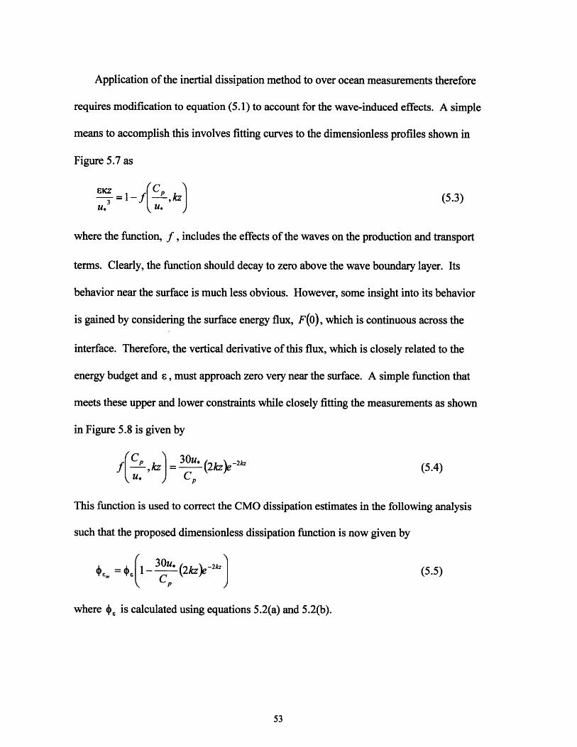
Application of the inertial dissipation method to over ocean measurements therefore

requires modification to equation (5.1) to account for the wave-induced effects. A simple

means to accomplish this involves fitting curves to the dimensionless profiles shown in

Figure 5.7 as

z = 1- f , kz) (5.3)

where the function, f, includes the effects of the waves on the production and transport

terms. Clearly, the function should decay to zero above the wave boundary layer. Its

behavior near the surface is much less obvious. However, some insight into its behavior

is gained by considering the surface energy flux, F(O), which is continuous across the

interface. Therefore, the vertical derivative of this flux, which is closely related to the

energy budget and s, must approach zero very near the surface. A simple function that

meets these upper and lower constraints while closely fitting the measurements as shown

in Figure 5.8 is given by

3C 30u (2kz)e- 2 (5.4)

u.' C

This function is used to correct the CMO dissipation estimates in the following analysis

such that the proposed dimensionless dissipation function is now given by

= I u- (2kz)et2k (5.5)

where 4, is calculated using equations 5.2(a) and 5.2(b).

SC u. < 24

24 < C/u. < 28

28 < C /u. < 32P

1 32 < C/u. < 37

$ 37<C/u. <50

50 < Cp/u. < 180

/I/I

/I

'I/

I I

/

/

- - - - +3 -- ---

/-

-------'-~

/

~

/O

o~~ .- A-

0.6 0.7

SK z / [u (zL)]

Figure 5.8 Ratio of predicted to measured dissipation rates versus non-dimensional

height for six wave-age bins. The curves represent the function f = 30u* (2kz -2k andCP

the error bars denote the standard error. The symbols are the same as in Figure 5.7.

2.2 F

1.8

1.6

1.4

1.2

1

0.8

0.6 H

0.4 -

0.2 + -- - - _

0.4 0.5 0.8 0.9I I I I I I I I

_ --- _ --- /-°

-i O-

/.I

/i ',--,

The modified inertial dissipation estimates are compared to the original dissipation

estimates and the direct covariance measurements of the friction velocity in Figure 5.9.

Whereas the previous inertial dissipation method systematically under predicted the

momentum flux, the new parameterization improves the estimates substantially. The

mean deviation of the inertial dissipation values calculated from the previous model was

0.049 m/s. The estimates calculated from the proposed inertial dissipation method

deviate by one-third the previous error; i.e., the mean deviation is only 0.032 m/s. Thus,

employing the new parameterization results in over a 33% reduction in the error

associated with calculating friction velocity estimates using the inertial dissipation

method.

Importantly, the new parameterization, , , was developed using an independent

data set measured over open-ocean conditions of unlimited fetch and depth. This

suggests the universality of the modified function and serves as satisfactory validation of

the parameterization. That is, the parameterization has not been "tuned" to fit the CMO

measurements, but rather was developed independently and found to result in impressive

improvement of the dissipation method when compared to the motion-corrected direct

covariance measurements.

5.4. MODIFIED BULK AERODYNAMIC METHODS

The approach proposed in this section is based upon the ideas, presented in section

4.2.2, that Charnock's expression for the surface roughness, z, accounts for the

roughness of the short gravity-capillary waves. However, modifications of the drag due

to gravity waves and swell are not included in standard bulk formula. To improve drag

coefficient estimates and, therefore, wind stress estimates in the bulk aerodynamic model,

Friction Velocity u. Comparison

0.1 0.2 0.3 0.4 0.5 0.6 0.7Direct Covariance u. (m/s)

Figure 5.9 Friction velocity, u., comparison for original and proposed inertial

dissipation methods and direct covariance method. Symbols: o Proposed inertialdissipation method; x Original inertial dissipation method. Data are bin averagedin increments of 0.02 m/s.

0.8

0.7

0.6

E 0.5

0.2

0.1

00.8

we need to relate the total drag (short plus long waves) to wave parameters in a

quantitative manner.

The goal of directly relating the sea surface drag coefficient to sea state has remained

elusive (Smith et al., 1992; Dobson et al., 1994). Donelan (1982) was one of the first to

present field data which showed a strong relationship between wave parameters and wind

stress. His research demonstrated the breakdown of Charnock's relation between the

aerodynamic roughness length and the friction velocity in all but fully-developed wave

conditions.

Since this pioneering work, other researchers have attempted to define a quantitative

relationship between the wind and wave fields. Smith (1991) demonstrated a "drag

coefficient anomaly," a departure of the drag coefficient from values expected through the

use of Charnock's expression, which was significantly correlated with wave age:

C103 ACDN = 1.85 - 2.24 cp (5.5)

(UlION cos)

where C, and UON are expressed in ms4' and 0 is the difference between the wind and

wave directions. Geernaert et al. (1986) proposed an empirical relation between wind

stress and wave age; however, lacking wave spectral data, they were forced to estimate

the wave field from wind data and may have predetermined their results on account of

this circular argument. Following the ideas of Kitaigorodskii (1973) and Janssen (1989),

Nordeng (1991) proposed a "wave age dependent Charnock constant":

g r= z. f C (5.6)

However, this approach cannot convincingly stand alone since u. appears in both z. and

the wave age, and self-correlation may produce spurious results (Hicks, 1978; Dobson

et al., 1994).

5.4.1. SCALING ROUGHNESS LENGTH WITH WAVE AMPLITUDE

An alternate approach, which is explored here, is derived from Donelan et al. (1993).

The aerodynamic roughness length is scaled by the rms amplitude a of the waves, where

a is defined in terms of the significant wave height, H, as 40 = H and where z

expresses the ability of the waves to serve as roughness elements (Donelan, 1990). The

benefit of regressing the ratio of z to inverse wave age is that the dimensionless ratios

are formed from four independent parameters, and the regression avoids the problem of

self-correlation by estimating the sea surface roughness from wave age parameters (a

and Cp ) that can be measured in situ (Smith et al., 1992).

Since the idea that the roughness length should be correlated with the height of the

waves depends on the concept of rough aerodynamic flow, attention is limited to cases for

which U10 > 7.5 m/s (Wu, 1980; Donelan, 1990). Thus, the following roughness length

determination applies only to fully rough flow. This formulation does not apply to cases

for which the surface layer appears to be aerodynamically smooth, U10 < 3 m/s, or to

transitional flow.

As depicted in Figure 5.10, inverse wave-age estimates from the modified inertial

dissipation method exhibit an increase of roughness scaled with rms wave height, as

expressed quantitatively by the regression line

- 2.7

= 9.6 x 10-4 UIN (5.7)o CP

which displays good agreement to the regression line

z = 5.5 x 10-4 1ON (5.8)G C,

fitted to data obtained in 12 m of water on Lake Ontario (Donelan et al., 1993) and agrees

well to the [(UON /C )3] power law obtained by Smith et al. (1992) from data obtained

during the Humidity Exchange over the Sea (HEXOS) experiment in 18 m of water over

the North Sea. In contrast, Dobson et al. (1994) found a weaker U[(UlO/Cp )7] power

law for data obtained during the Grand Banks ERS-1 SAR Wave Validation Experiment.

However, the scatter in their data set did not allow them to resolve the slope (power law)

well, and they indicate that a neutral or two way regression would give a steeper

[UON /C p 5 ] power law, which would be in better agreement with the power laws

obtained using the CMO, Lake Ontario, and North Sea data sets. The close agreement in

the power laws obtained in four independent experiments, which ranged in environmental

conditions from lake to open ocean, suggests the strength of the relationship between the

surface roughness length, the rms height of the dominant seas and the wave age, as

expressed in equation (5.7).

In Figure 5.11, the CMO rms wave height measurements are empirically related to

the wave age and wind speed by the regression line

2g2 o3UIoN-18-2 2 = 2.9 x 10-3 U(5.9)

(UcosO)4 C

Regression based on Modified Inertial Dissipation Estimates

-1

U /Cp

100

Figure 5.10 The ratio of measured roughness length z, to rms wave height a versusinverse wave age U 0o / C,, binned in increments of log(0.035). Symbols: . CMOdata; - regression on present data, equation (5.7); --- Dobson et al. (1994);- - Donelan et al. (1993), equation (5.8); - - - - Smith et al. (1992).

10"2

10

0N

104

10-s

10

//

// -

/4-'

/ /// /

/ /

1 I I

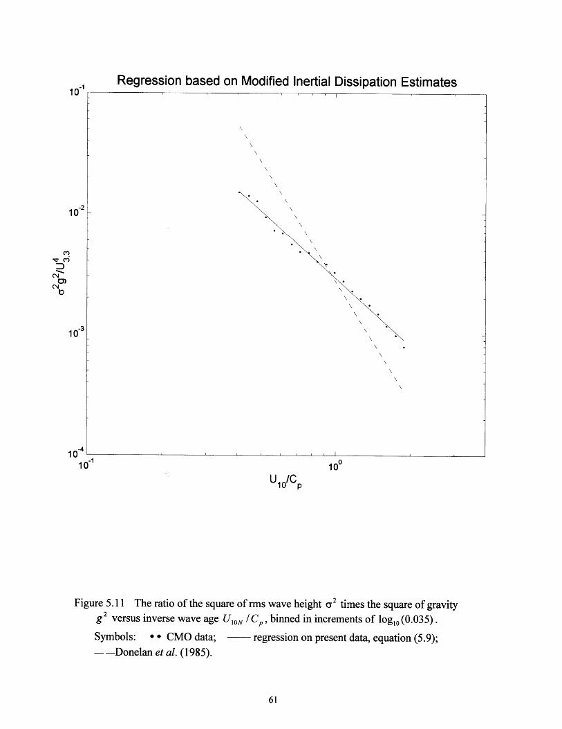
Figure 5.11

Regression based on Modified Inertial Dissipation Estimates

U p/Cp

100

The ratio of the square of rms wave height a 2 times the square of gravityg2 versus inverse wave age U10N /IC, binned in increments of log10 (0.035).

Symbols: * * CMO data; - regression on present data, equation (5.9);- -Donelan et al. (1985).

10 1

10-2

10

10-410

-1

where g is the acceleration of gravity and 0 is the angle between the winds and the

waves. Donelan et al. (1985) found a steeper [(UION/C )- 3 3] relationship using their

Lake Ontario field data. Examination of Figure 5.11 reveals that the regression used to

obtain equation (5.9) is a relatively tight fit. The marked difference between the power

laws derived from the Lake Ontario and CMO data sets is a reflection of the different

environmental regimes, the data from Donelan et al. (1985) representing shallow lake

conditions and our data representing ocean conditions over the continental shelf. These

differences can include, for example, a dependence on fetch that is felt at the lake site but

not at the CMO site.

Assuming that the wind and wave fields are aligned at the surface (cos0 ;z 1),

equation (5.9) may be simplified

2- 2 U" I - 0.92

r= 5.4 x / (5.10)L g C,

Substituting the expression for the rms wave height, equation (5.11), into equation

(5.7) provides an expression for the roughness length

S2u 1.8

Zr = 5.2 x 10-' l[ (5.11)

which has a steeper power law than the expression derived by Donelan et al. (1993)

-0.9

zr =3.7x 1 (5.12)

due to the different empirical relationship for the dependence of the wave height on wind

speed. Equation (5.11) implies that the roughness length depends quadratically on the

wind and wave-age. However, as mentioned, this relationship for the roughness length is

only applicable to the same type of ocean conditions present at the CMO site because the

parameterizations do not give the same rms wave height, a, for the same wind speed and

wave age. This severely limits the widespread application of this type of

parameterization. Thus, it is preferable to return to equation (5.7) which appears to be a

more robust relationship since the scaling gives similar results under similar conditions at

all sites.

Equation (5.7) is now used in the bulk aerodynamic method as an alternate means of

calculating the roughness length. It was hypothesized that including sea state dependence

into drag coefficient calculations would improve the wind stress estimates, particularly in

the case of young (developing) seas. Friction velocity estimates calculated by the

modified bulk method are depicted in Figure 5.12. Overall, the new parameterization

slightly improves the u. estimates when compared to their former values, although the

difference is not statistically significant. Of note, the modified bulk method results in

higher friction velocity estimates than the original method for all wind speeds

u. > 0.2 m/s, and the new parameterization produces estimates that over predict the actual

momentum flux for u. > 0.3 m/s. Although statistically the modified bulk aerodynamic

method yields the same error as the original method, the trend is significantly different.

Whereas the original method tended to over predict the momentum flux over decaying

seas and underestimate the flux over developing seas, the modified method tends to over

predict the flux for all wave ages, which suggest that there is an inherent bias in the

correction.

Friction Velocity u. Comparison

0.1 0.2 0.3 0.4 0.5 0.6Direct Covariance u. (m/s)

0.7 0.8 0.9

Figure 5.12 Friction velocity, u., comparisons of the bulk aerodynamic versus motion-corrected covariance method for the original bulk method (+) and the modifiedparameterization (o). Values of u. are bin-averaged in increments of 0.02 m/s.

0.9

0.8

0.7

-0.6

E

o 0.5ECc

m 0.3

0.2

0.1

0

One limitation of this model is the log-linear regression required by equation (5.7).

A closer inspection of Figure 5.11 reveals that the points indicate that either a curve or

two different linear regressions would more adequately estimate z' . Additionally, noticea

that the young seas, i(o P -1 only represent about 10% of the total data, yet tend to

increase the slope (power law) significantly. In fact, when only the young data is

considered, the power law increases to [(UION /C, 3.0 ], whereas if only the fully-

developed and decaying seas are considered, the slope decreases to [(UION/C )- 2.

Notice that these results are within the span of ranges found by other researchers (Smith

et al., 1992; Donelan et al., 1993;; Dobson et al., 1994) and could, in part, explain the

differences that are found.

In Figure 5.13, the new bulk aerodynamic estimates are compared to direct

covariance drag coefficient measurements. In contrast to the bulk estimates in Figure 5.4,

the modified roughness length calculation results in sea state dependent drag coefficients;

for a given wind speed, the predicted drag coefficient is inversely related to wave-age.

However, the tendency of the [(UION /C, )-2.7 ] power law to overestimate the friction

velocity results in higher than expected drag coefficients for all wave ages and wind

speeds.

5.4.2. MODIFIED CHARNOCK'S RELATION

The overall goal is to provide the best momentum flux estimates for the Coastal

Mixing and Optics experiment. While the results obtained using the approach of Donelan

et al. (1993) are promising, the new estimates are not significantly improved over the

Drag Coefficient vs Wind Speed Comparison

C /u.<=24

+-t+-t- ++

+++ T+T)

5 10 15 20U Oin m/s

28<C /u.<=32

+ + + ++

5 10 15 20Uo N in m/s

2.5

a

xz.5

1

0.5

2.5

2

x 1.5

1

0.5

2.5

2

x 1.5

0.5 0.5

24<C pu.<=28p

5 10 15 20Ulo in m/s

32<C pu.

+++

5 10 15 20UlONin mis

+ Bulk Aerodynamico Direct Covariance

Figure 5.13 A comparison of the neutral drag coefficient CDN estimated using the

modified bulk aerodynamic method and compared to motion-corrected covariance

measurements (averaged in increments of 1 m/s) for four different wave-age S bins.

The error bars for the covariance measurements denote the standard error.

J+++

2.5

0

1xUC.

previous values. Furthermore, the parameterization tends to overestimate the roughness

length for all wind speeds, a trend which indicates an inherent bias in the model. Thus,

still in pursuit of a means to reconcile the current deficiency of the bulk aerodynamic

method to estimate the wind stress in cases of young (developing) seas, but not to

overestimate the wind stress in cases of fully-developed or decaying seas, another method

of forcing a wave-age dependence into the roughness length via the Chamock's

"constant" is explored. On the basis of the direct covariance measurements, the

Charnock's "constants" that provided the best fits for young, fully-developed, and

decaying seas are a c = 0.0150, ac = 0.0126 and ac = 0.0059, respectively. Figure 5.14

shows the measured Charnock's parameter as a function of wave age, for which the

function

~ = -4.05 x 10-4(P ) + 2.34 x 10-2 (5.13)

provides the best linear regression. Revisiting equation (4.19), the approach of Smith

(1988) is modified

zo = z, + Zr (5.14)

where z s is determined as before [equation (4.20)], but z, is now expressed as

2

Zr =ac-g

where

S= -4.05 x 10-4 + 2.34 x 10-2 for < 43 (5.15)

C) a Measured ac_4 0-2a =-4.05x10 - (C p/U.) + 2.34x10 2

c p

01 1 I I I

5 10 15 20 25 30 35Wave Age C lu.

Figure 5.14

40 45 50 55

Estimated wave age dependent Charnock's "constant":

c = -4.05 x 10-4, P + 2 .34 x 10-2.(u*

0.02

0.018

0.016

0.014

0.012

0.01

0.008

0.006

0.004

0.002-

c;

CpFor seas with wave ages older than ' >2 43, the Charnock's parameter is assigned the

value of ac = 0.0059, the value of the upper limit.

The modified Charnock's parameterization results in improved friction velocity

estimates, as illustrated in Figure 5.15. Whereas the original bulk estimates had a mean

deviation of 0.046 m/s, the new parameterization reduces the error by 7% and results in a

mean deviation of 0.043 m/s. While this may seem small, the subsequent improvement in

the drag coefficient estimates (Figure 5.16) is quite noticeable. Previously, the bulk

aerodynamic method underestimated the drag associated with young seas, but now the

estimates are in good agreement with the direct covariance measurements. For the

remaining three wave-age bins, the modified Charnock's expression again provides

improved estimates of the drag over fully-developed and decaying seas. These results

suggest that there is a benefit to incorporating wave-age dependence into the bulk

aerodynamic model, even if the forcing is as simple as including a wave-age dependent

Charnock's parameter. Obviously, further research is required to validate the function

proposed here, especially since the wave-age span is limited: the youngest seas averaged

CP 20, and the oldest seas averaged C - 43, providing a somewhat limited rangeU* U,

upon which the proposed function is based. Thus, while the relationship proposed here

improves the bulk aerodynamic momentum flux estimates for the CMO experiment,

future studies are needed to validate or improve the parameterization. Most importantly,

the results indicate that bulk aerodynamic momentum flux estimates can be improved by

incorporating sea state dependence via a roughness length determination.

Friction Velocity u. Comparison0.9

0.8

0.7

' 0.6

E

.2 0.5Ecc

20.4

75m 0.3

0.2

0.1

00.9

Figure 5.15 Friction velocity, u., comparisons of the bulk aerodynamic versus motion-corrected covariance method for the original bulk method (+) and the modified-Charnock parameterization (o). Values of u. are bin-averaged in increments of0.02 m/s.

0.1 0.2 0.3 0.4 0.5 0.6 0.7 0.8Direct Covariance u. (m/s)

Drag Coefficient vs Wind Speed Comparison

C /u.<=24

2.5

2

x 1.5z

1

0.5

2.5

2

2.5

2

x 1.5

1

0.5

2.5

2

xzo0

0.515

U ION in m/s

24<C /u.<=28p

5 10 15 20U ION in mrn/s

32<C /u.

5 10 15 20U N in m/s

ION

+ Bulk Aerodynamico Direct Covariance

Figure 5.16 A comparison of the neutral drag coefficient CDN estimated using the

modified-Charnock bulk aerodynamic method and compared to motion-correctedcovariance measurements (averaged in increments of 1 m/s) for four different wave-

age L bins. The error bars for the covariance measurements denote the standard

error.

j) + +±

5 10 15 20U ION in mrn/s

28<Cp /u<=32p

oxlz

0

0.5

++ + ()

6. CONCLUSIONS

The work presented in this thesis is an investigation of the influence of surface waves

on momentum exchange. Accurate measurements of the exchange of momentum and

energy between the atmosphere and ocean are critical to numerical prediction systems.

The growing sophistication of current numerical models, such as the United States

Navy's Coupled Ocean Atmosphere Prediction System, requires an accurate

representation of the dynamics and magnitude of energy transfer through the air-sea

interface. This thesis explored the theoretical framework which forms the basis for the

direct covariance (eddy correlation), direct / inertial dissipation and bulk aerodynamic

methods for measuring and calculating momentum flux. Unlike the other methods which

rely on similarity theory, the direct covariance method provides a direct computation of

the wind stress. However, this method is highly susceptible to flow distortion and

platform motion and is, therefore, difficult to implement in over-ocean studies. It is

therefore preferable to develop indirect methods such as the bulk aerodynamic and

inertial dissipation methods which relate easily measured quantities such as wind speed

and temperature to the momentum flux. These methods allow us to estimate turbulent

quantities when direct measurements are unavailable and to estimate the lower boundary

flux conditions to input into numerical models.

The indirect methods for estimating momentum exchange rely on Monin-Obukhov

similarity theory, which was developed almost half a century ago and has been validated

over land by a number of field experiments. Its applicability over the ocean has only

recently been examined. By quantitatively comparing the bulk and inertial dissipation

estimates to direct measurements, it was determined that the indirect methods

systematically underestimate the momentum flux into developing seas. It was

hypothesized that incorporating sea state dependence into the parameterizations would

improve the wind stress estimations computed from both methods.

For the inertial dissipation method, a new parameterization for the dimensionless

dissipation rate that includes the effects of the surface waves and accounts for the non-

zero flux of energy from the atmosphere to the ocean is proposed:

= - (2kz-I2kz (6.1)

This parameterization was developed from an independent data set and has resulted in

over a 33% reduction of the error associated with the inertial dissipation friction velocity

estimates when compared to direct covariance measurements.

Two separate methods of incorporating sea state dependence into the bulk

aerodynamic method were explored. The first parameterization is based on the ideas of

Donelan et al. (1993) and involved the derivation of a sea surface roughness length

normalized by rms wave height that is a log-linear function of wave age:

z = 9.6 x 10- 4 o (6.2)a C

This parameterization agrees well with the relationships presented by Smith et al. (1992)

and Donelan et al. (1993).

The parameterization was used in the bulk aerodynamic method and slightly

improves the friction velocity estimates, although the difference is not statistically

significant. The results indicate, however, an inherent bias and systematic trend in

overestimating u.. One limitation is the lack of data with young wave ages so that the

power law cannot be resolved well in the lower limit. Another possibility is that the log-

linear relationship is too simplistic; the data suggest that a curve, or at least two lines,

would provide a more optimal fit.

The second approach to modifying the bulk aerodynamic method involved

incorporating a sea state dependent Charnock's parameter into the roughness length

calculation:

2

Zr = acU (6.3a)

where

a= -4.05 10 4 +2.34 x 10-2 (6.3b)

for C'< 43.u

When compared to the direct covariance measurements, this new parameterization

resulted in a 7% reduction in the error associated with bulk aerodynamic friction velocity

estimates and considerably improved drag coefficient estimates. The results are tentative

due to the limited wave-age span upon which the function is derived, and more research

is needed to validate or improve the shape of the function, especially in both the upper

and lower limits.

Finally, this research strongly supports the use of either the bulk aerodynamic or

inertial dissipation methods to estimate momentum exchange over the ocean. Since

widespread direct measurements are not practical, indirect methods such as the bulk and

inertial dissipation methods are invaluable. While future research will undoubtedly

improve the accuracy of both methods, especially as we gain increased understanding of

wind-wave coupling, the results obtained here indicate that the current bulk aerodynamic

and inertial dissipation algorithms which already have widespread acceptance are, in fact,

doing an adequate job of estimating the momentum flux. This investigation provides

strong quantitative evidence that incorporating sea state dependence into both methods

takes us one step closer and improves upon current momentum flux estimates.

76

REFERENCES

Anctil, F., M. A. Donelan, W. M. Drennan, and H. C. Graber, 1994: Eddy-correlationmeasurements of air-sea fluxes from a discus buoy. Journal ofAtmospheric andOceanic Technology, 11, 1144-1150.

Barstow, S. F., G. Ueland, H. E. Krogstad, and B. A. Fossum, 1991: The wavescansecond generation directional wave buoy. IEEE Journal of Oceanic Engineering, 16,254-266.

Baumgartner, M. F. and S. P. Anderson, 1997: Acquisition, Description and EvaluationofAtmospheric Model Products for the Coastal Mixing and Optics Experiment.Woods Hole Oceanographic Institute Technical Report, WHOI-97-02, 1-29.

Bradley, E. F., P. A. Coppin, and J. S. Godfrey, 1991: Measurements of sensible andlatent heat flux in the western equatorial Pacific Ocean. Journal of GeophysicalResearch, 96, 3375-3389.

Businger, J. A., 1973: Turbulent transfer in the atmospheric surface layer. Workshop onMicrometeorology, D. A. Haugen, Ed., American Meteorological Society, 67-100.

Businger, J. A., J. C. Wyngaard, Y. Izumi, and E. F. Bradley, 1971: Flux-profilerelationships in the atmospheric surface layer. Journal of the Atmospheric Sciences,28, 181-189.

Charnock, H., 1955: Wind stress on a water surface. Quarterly Journal of the RoyalMeteorological Society, 81, 639.

Davidson, K. L., C. E. Skupniewicz, D. Ross, R. G. Onstott, J. A. Johannessen, andO. Skagseth, 1991: Relationship between wind stress, backscatter, and the directionalwave spectrum (NORCSEX-88). Proceedings of OCEANS '91, Honolulu, HI, IEEE,998-1005.

Dobson, F. W., S. D. Smith, and R. J. Anderson, 1994: Measuring the relationshipbetween wind stress and sea state in the open ocean in the presence of swell.Atmosphere-Ocean, 32, 237-256.

Donelan, M. A., 1982: The dependence of the aerodynamic drag coefficient on waveparameters. Proceedings of the I"s International Conference on Meteorology and Air-Sea Interaction of the Coastal Zone, the Hague, American Meteorological Society,381-387.

Donelan, M. A., 1990: Air-sea interaction. In The Sea (eds. B. LeMdhaut6 andD. M. Hanes). Wiley-Interscience, New York, 239-292.

Donelan, M. A., J. Hamilton, and W. H. Hui, 1985: Directional spectra of wind-generated waves. Phil. Trans. Roy. Soc. London A, 315, 509-562.

Donelan, M. A., F. W. Dobson, S. D. Smith, and R. J. Anderson, 1993: On thedependence of sea surface roughness on wave development. Journal of PhysicalOceanography, 23, 2143-2149.

Dugan, J. P., S. L. Panichas, and R. L. DiMarco, 1991: Decontamination of windmeasurements from buoys subject to motions in a seaway. Journal ofAtmosphericand Oceanic Technology, 8, 85-95.

Dyer, A. J., 1974: A review of flux-profile relationships. Boundary Layer Meteorology,7, 363-372.

Dyer, A. J. and B. B. Hicks, 1982: Kolmogorov constants at the 1976 ITCE. BoundaryLayer Meteorology, 22, 137-150.

Earle, D. M. and J. M. Bishop, 1984: A Practical Guide to Ocean Wave Measurementand Analysis. ENDECO, Inc., Marion, MA, 78 pp.

Edson, J. B., C. W. Fairall, P. G. Mestayer, and S. E. Larsen, 1991: A study of theinertial-dissipation method for computing air-sea fluxes. Journal of GeophysicalResearch, 96, 10689-10711.

Edson, J. B., S. Wetzel, C. Friehe, S. Miller, and T. Hristov, 1997: Energy flux anddissipation profiles in the marine surface layer. Proceedings of the 1 2th Symposium onBoundary Layers and Turbulence, Vancouver, BC, Canada, American MeteorologicalSociety, 314-315.

Edson, J. B., A. A. Hinton, K. E. Prada, J. E. Hare, and C. W. Fairall, 1998: Directcovariance flux estimates from mobile platforms at sea. Journal ofAtmospheric andOceanic Technology, 15, 547-562.

Edson, J. B. and C. W. Fairall, 1998: Similarity relationships in the marine atmosphericsurface layer for terms in the TKE and scalar variance budgets. Journal of theAtmospheric Sciences, 55, 2311-2328.

Fairall, C. W. and S. E. Larsen, 1986: Inertial-dissipation methods and turbulent fluxes atthe air-ocean interface. Boundary Layer Meteorology, 34, 287-301.

Fairall, C. W., J. B. Edson, S. E. Larsen, and P. G. Mestayer, 1990: Inertial-dissipationair-sea flux measurements: a prototype system using realtime spectral computations.Journal ofAtmospheric and Oceanic Technology, 7, 425-453.

Fairall, C. W., E. F. Bradley, D. P. Rogers, J. B. Edson, and G. S. Young, 1996a: Bulkparameterization of air-sea fluxes for Tropical Ocean-Global Atmosphere Coupled-Ocean Atmosphere Response Experiment. Journal of Geophysical Research, 101,3747-3764.

Fairall, C. W., E. F. Bradley, J. S. Godfrey, G. A. Wick, J. B. Edson, and G. S. Young,1996b: Cool-skin and warm-layer effects on sea surface temperature. Journal ofGeophysical Research, 101, 1295-1308.

Fairall, C. W., A. B. White, J. B. Edson, and J. E. Hare, 1997: Integrated shipboardmeasurements of the marine boundary layer. Journal ofAtmospheric and OceanicTechnology, 14, 338-359.

Finnigan, J. J., F. Einuadi, and D. Fua, 1984: The interaction between an internal gravitywave and turbulence in the stably-stratified nocturnal boundary layer. Journal ofAtmospheric Sciences, 41, 2409-2436.

Frederickson, P. A., K. L. Davidson, and J. B. Edson, 1997: A study of wind stressdetermination methods from a ship and an offshore tower. Journal ofAtmosphericand Oceanic Technology, 14, 822-834.

Frenzen, P. and C. A. Vogel, 1992: The turbulent kinetic energy budget in theatmospheric surface layer: a review and an experimental reexamination in the field.Boundary Layer Meteorology, 60, 49-76.

Fujitani, T., 1981: Direct measurement of turbulent fluxes over the sea during AMTEX.Papers in Meteorology and Geophysics, 32, 119-134.

Fujitani, T., 1985: Method of turbulent flux measurement on a ship by using a stableplatform system. Papers in Meteorology and Geophysics, 36, 157-170.

Galbraith, N., W. Ostrom, B. Way, S. Lentz, S. Anderson, M. Baumgartner,A. Plueddemann, and J. Edson, 1997: Coastal Mixing and Optics Experiment:Mooring Deployment Cruise Report. Woods Hole Oceanographic Institute TechnicalReport, WHOI-97-13, 81 pp.

Garratt, J. R., 1992: The Atmospheric Boundary Layer. Cambridge University Press,New York, 316 pp.

Geernaert, G. L., 1990: Bulk parameterizations for the wind stress and heat fluxes. InSurface Waves and Fluxes, Volume I (eds. G. L. Geernaert and W. J. Plant). KluwerAcademic Publishers, Boston, 91-172.

Geernaert, G. L., K. B. Katsaros, and K. Richter, 1986: Variation of the drag coefficientand its dependence on sea state. Journal of Geophysical Research, 91, 7667-7679.

Geernaert, G. L., S. E. Larsen, and F. Hansen, 1987: Measurements of the wind stress,heat flux, and turbulence intensity during storm conditions over the North Sea.Journal of Geophysical Research, 92, 13127-13139.

Geernaert, G. L., K. L. Davidson, S. E. Larsen, and T. Mikkelsen, 1988: Wind stressmeasurements during the Tower Ocean Wave and Radar Dependence Experiment.Journal of Geophysical Research, 93, 13913-13923.

Gill, A. E., 1982: Atmosphere-Ocean Dynamics. Academic Press, San Diego, 662 pp.

Hare, J. E., J. B. Edson, E. J. Bock, and C. W. Fairall, 1992: Progress on directcovariance measurements of air-sea fluxes from ships and buoys. Tenth Symposiumon Turbulence and Diffusion, Portland, OR, American Meteorological Society, 281-284.

Henjes, K., P. K. Taylor, and M. J. Yelland, 1998: Effect of pulse averaging on sonicanemometer spectra. Journal ofAtmospheric and Oceanic Technology, in press.

Hicks, B. B., 1978: Some limitations of dimensional analysis and power laws.Boundary-Layer Meteorology, 14, 567-569.

Hicks, B. B. and A. J. Dyer, 1972: The spectral density technique for determination ofeddy fluxes. Quarterly Journal of the Royal Meteorological Society, 98, 838-844.

Hill, R. J., 1996: Corrections to Taylor's frozen turbulence approximation. AtmosphericResearch, 40, 153-175.

H6gstr6m, U., 1987: Non-dimensional wind and temperature profiles in the atmosphericsurface layer: a re-evaluation. Boundary Layer Meteorology, 42, 55-78.

H6gstr6m, U., 1996: Review of some basic characteristics of the atmospheric surfacelayer. Boundary Layer Meteorology, 78, 215-246.

Janssen, P. A. E. M., 1989: Wave-induced stress and the drag of air flow over sea waves.Journal of Physical Oceanography, 19, 745-754.

Kaimal, J. C., J. C. Wyngaard, and D. A. Haugen, 1968: Deriving power spectra from athree-component sonic anemometer. Journal ofApplied Meteorology, 7, 827-837.

Kitaigorodskii, S. A., 1973: The Physics ofAir-Sea Interaction, translated from Russian,Israel Program for Scientific Translations, Jerusalem, 237 pp.

Large, W. G. and J. A. Businger, 1988: A system for remote measurements of the windstress over the ocean. Journal ofAtmospheric and Oceanic Technology, 5, 274-285.

Large, W. G. and S. Pond, 1981: Open ocean momentum flux measurements of the windstress over the ocean. Journal of Physical Oceanography, 11, 324-336.

Lumley, J. L. and H. A. Panofsky, 1964: The Structure ofAtmospheric Turbulence.J. Wiley and Sons, New York, 229 pp.

Maat, N., C. Kraan, and W. A. Oost, 1991: The roughness of wind waves. BoundaryLayer Meteorology, 54, 89-103.

Mahrt, L., D. Vickers, J. Howell, J. Hojstrup, M. Courtney, J. M. Wilczak, J. B. Edson,

and J. Hare, 1996: Sea surface drag coefficients in Ris0 Air Sea Experiment(RASEX). Journal of Geophysical Research, 101, 14327-14335.

Miller, M. J., A. C. M. Beljaars, and T. N. Palmer, 1992: The sensitivity of the ECMWFmodel to the parameterization of evaporation from the tropical oceans. Journal ofClimate, 5, 418-434.

Monin, A. S. and A. M. Obukhov, 1954: Basic laws of turbulent mixing in the surfacelayer of the atmosphere. Trudy Geofizicheskogo Instituta Akademiya Nauk SSSR,24,163-187.

Nordeng, T. E., 1991: On the wave age dependent drag coefficient and roughness lengthat sea. Journal of Geophysical Research, 96, 7167-7174.

Panofsky, H. A. and J. A. Dutton, 1984: Atmospheric Turbulence. Wiley-Interscience,New York, 397 pp.

Shaw, W. J., 1990: Theory and scaling of lower atmospheric turbulence. In SurfaceWaves and Fluxes, Volume I (eds. G. L. Geernaert and W. J. Plant). Kluwer AcademicPublishers, Boston, 63-72.

Smith, S. D., 1980: Wind stress and heat flux over the ocean in gale force winds.Journal of Physical Oceanography, 10, 709-726.

Smith, S. D., 1988: Coefficients for sea surface wind stress, heat flux, and wind profilesas a function of wind speed and temperature. Journal of Geophysical Research, 93,15467-15472.

Smith, S.D., 1991: Some early results of the Humidity Exchange over the Sea mainexperiment. In Deep Convection and Deep Water Formation in the Oceans (eds.P. C. Chu and J. C. Gascard). Elsevier Science Publishers, Amsterdam, 377-382.

Smith, S.D., R. J. Anderson, W. A. Oost, C. Kraan, N. Maat, J. DeCosmo,K. B. Katsaros, K. L. Davidson, K. Bumke, L. Hasse, and H. M. Chadwick, 1992: Seasurface wind stress and drag coefficients: The HEXOS results. Boundary LayerMeteorology, 60, 109-142.

Smith, S. D., C. W. Fairall, G. L. Geernaert, and L. Hasse, 1996: Air-sea fluxes: 25 yearsof progress. Boundary Layer Meteorology, 78, 247-290.

Stenner, R., 1996: Coastal Mixing and Optics Experimental Site(http://wavelet.apl.washington.edu/CMO/CMO_bath.html).

Thiermann, V. and H. Grassl, 1992: The Measurement of turbulent surface layer fluxesby use of Bichromatic Scintillation. Boundary Layer Meteorology, 58, 367-389.

Tsukamoto, O., E. Ohtaki, H. Ishida, M. Horiguchi, and Y. Mitsuta, 1990: On-boarddirect measurements of turbulent fluxes over the open sea. Journal of theMeteorological Society ofJapan, 68, 203-211.

Vogel, C. A. and P. Frenzen, 1992: A new study of the TKE budget in the surface layer,Part II: The dimensionless function and divergent transport terms. Proceedings of the10th Symposium on Turbulence and Diffusion, Portland, OR, American MeteorologicalSociety, 161-164.

Wallace, J. M. and P. V. Hobbs, 1977: Atmospheric Science. Academic Press,San Diego, 467 pp.

Webb, E. K., G. I. Pearman, and R. Leuning, 1980: Correction of flux measurements fordensity effects due to heat and water vapor transport. Quarterly Journal of the RoyalMeteorological Society, 106, 85-100.

Webster, P. J. and R. Lukas, 1992: TOGA COARE: The Coupled Ocean AtmosphereResponse Experiment. Bulletin American Meteorological Society, 73, 1377-1416.

Weller, R. A., D. L. Rudnick, R. E. Payne, J. P. Dean, N. J. Pennington, and R. P. Trask,1990: Measuring near-surface meteorology over the ocean from an array of surfacemoorings in the subtropical convergence zone. Journal ofAtmospheric and OceanicTechnology, 7, 85-103.

Williams III, A. J., 1997: Introduction. Coastal Mixing and Optics Report III,Proceedings of the Coastal Mixing and Optics Meeting, Santa Fe, NM, 13 9 pp.

Wu, J., 1980: Wind-stress coefficients over sea surface near neutral conditions-arevisit. Journal of Physical Oceanography, 10, 727-740.

Wyngaard, J. C., 1973: On surface layer turbulence. Workshop on Micrometeorology,D. A. Haugen, Ed., American Meteorological Society, 101-149.

Wyngaard, J. C. and S. F. Clifford, 1977: Taylor's Hypothesis and high frequencyturbulence spectra. Journal of the Atmospheric Sciences, 34, 922-928.

Yelland, M. J., P. K. Taylor, I. E. Consterdine, and M. H. Smith, 1994: The use of theinertial dissipation technique for shipboard wind stress determination. Journal ofAtmospheric and Oceanic Technology, 11, 1093-1108.

Yelland, M. J. and P. K. Taylor, 1996: Wind stress measurements from the open ocean.Journal of Physical Oceanography, 26, 541-558.