Journal of Experimental Psychology; Human Perception and Performance 1995, Vol. 21, No. I, 183--202

Copyright 1995 by the American psYChoIOgi~~~~~/$3~

OBSERVATION

Why Change Gaits? Dynamics of the Walk-Run Transition

Frederick J. Diedrich and William H. Warren, Jr. Brown University

Why do humans switch from walking to running at a particular speed? It is proposed that gait transitions behave like nonequilibrium phase transitions between attractors. Experiment 1 examined walking and running on a treadmill while speed was varied. The transition occurred at the equal-energy separatrix between gaits, with predicted shifts in stride length and frequency, a qualitative reorganization in the relative phasing of segments within a leg, a sudden jump in relative phase, enhanced fluctuations in relative phase, and hysteresis. Experiment 2 dissociated speed, frequency, and stride length to show that the transition occurred at a constant speed near the energy separatrix. Results are consistent with a dynamic theory of locomotion in which preferred gaits are characterized by stable phase relationships and minimum energy expenditure, and gait transitions by a loss of stability and the reduction of energetic costs.

Motor behavior in humans and animals exhibits two no­table features: the presence of stable patterns of coordina­tion and the sudden reorganization that occurs when switch­ing between them. Much research has been directed at describing individual motor patterns such as walking and reaching, but the study of behavioral transitions may reveal principles of the formation of coordinative patterns. Loco­motion offers a model system for the study of both, for it is a fundamental, fluent, and complex behavior that is likely to share basic characteristics with other skilled actions. In this article, we examine the shift between walking and running in humans and offer a qualitative dynamic theory of gait transitions.

As speed increases, humans and other animals shift from a walking gait to a running gait at a characteristic speed. Why does this occur? A common view is that each gait is orchestrated by a central motor plan, such as a motor program or spinal pattern generator, and that gait transi­tions simply involve switching between plans (e.g., Shapiro, Zernicke, Gregor, & Diestel, 1981). This view does not offer predictions about the details of behavior at gait tran­sitions. By contrast, we propose that gait transitions are a consequence of the intrinsic dynamics of a complex system, with properties characteristic of bifurcations between attrac­tors. We show that the walk-run (W-R) transition exhibits features of a nonequilibrium phase transition and that it occurs at a speed that tends to reduce energetic costs. This

Frederick J. Diedrich and William H. Warren, Jr., Department of Cognitive and Linguistic Sciences, Brown University.

This research was supported by Grant AG05223 from the Na­tional Institutes of Health. We would like to thank Bruce Kay for his advice, as well as Ted Goslow, Dave Carrier, Michael Turvey, Ken Holt, and Gregor Schoner for their comments.

Correspondence concerning this article should be addressed to Frederick J. Diedrich, Department of Cognitive and Linguistic Sciences, Brown University, Providence, Rhode Island 02912. Electronic mail may be sent to diedrich@magnum.cog.brown.edu.

183

analysis is consistent with a general theory of pattern for­mation in complex physical and biological systems (Raken & Wunderlin, 1990; Kelso & Schoner, 1988), according to which coordinative patterns and transitions between them result from the nonspecific dynamics of the system rather than from a specific control process.

Theories of Gait Transitions

Recent models of bipedal gaits demonstrate that the basic features of walking and running could be produced by the passive dynamics of the limb system. In walking, the body behaves like an inverted pendulum (McGeer, 1990a; Mochon & McMahon, 1980), yielding highly conservative exchanges of kinetic and potential energy. In running, the body behaves like a bouncing ball, in which kinetic energy is converted to elastic energy stored in the tendons and muscles of the stance leg (Blickhan, 1989; McGeer, 1990b; McMahon & Cheng, 1990). A transition from the pendular walking mode to the elastic running mode could be brought about by an increase in propulsive force in the stance phase that propels the body into the air. This would yield charac­teristics of running such as a flight phase with no ground contact, the consequent storage of elastic energy in the leg upon landing, a reduced duty factor (stance time as a pro­portion of total stride time), and a ground reaction force profile that is single rather than double peaked.

Although individual gaits have been studied extensively, there is comparatively little research on gait transitions. In humans, the W-R transition typically occurs at a speed of about 2.1 mls (Beuter & Lalonde, 1989; Rreljac, 1993; our Experiment 1), although two studies have reported slightly lower means near 1.9 mls (Noble et aI., 1973; Thorstensson & Roberthson, 1987); the exact value may depend on sam­ple characteristics such as body size or athletic training. In quadrupeds, the trot-gallop transition occurs abruptly in one or two strides, although the walk-trot transition may

184 OBSERVATION

occur more gradually (see Vilensky, Libii, & Moore, 1991, for a review). The speed, frequency, and stride length at the trot-gallop transition scale allometrically with body size across a wide range of mammals (Heglund & Taylor, 1988; Heglund, Taylor, & McMahon, 1974), suggesting a physical basis for gait transitions. Alexander and Jayes (1983) equated transition speeds for different-size quadrupeds by normalizing speed v with respect to leg length L using the dimensionless Froude number F:

v 2

F=­Lg'

where g is acceleration due to gravity.

(1)

One possible explanation for gait transitions is that the shift to a new mode of progression occurs at the mechanical limit of the current mode (Alexander, 1984). Assuming that the stance leg is rigid during walking, the body's center of mass moves in an arc with a radius equal to leg length L, and the acceleration of the center of mass toward the foot is a = v21L. To keep the foot on the ground, this value cannot exceed the acceleration due to gravity, so the upper limit on walking speed is v < (gL)-O.5. Assuming a median leg length of 0.9 m, this model predicts a maximum walking speed of about 3.0 mis, much greater than the observed transition speed of 2.1 m/s.

A second explanation proposes that gait transitions occur in order to minimize total metabolic cost, known as an "energetic trigger." The transition is usually predicted from the speed at which the rate of energy expenditure for walk­ing (power, in calories per kilogram per second [callkgls]) surpasses that for running; this is equivalent to the speed at which running becomes more efficient than walking in terms of energy expenditure per unit distance (calories per kilogram per meter [callkglm]). Human data indicate this speed to be 2.2-2.3 mls (Falls & Humphrey, 1976; Marga­ria, 1976), close to the observed transition speed of 2.1 m/s. On the other hand, Hreljac (1993) reported that the preferred transition speed of 2.07 mls was statistically lower than the energetically optimal speed of 2.24 mls in the same indi­viduals; energy expenditure per meter at the transition speed was 16% higher in running than walking. This argues against a local energetic trigger, although as the runner accelerates the transition would soon act to reduce energetic costs.

A third hypothesis proposes that the shift is made to reduce mechanical stresses such as peak muscle force and bone strain, called a "mechanical trigger" (Farley & Taylor, 1991). They reported that loaded horses made the trot­gallop transition at a significantly lower speed than the energetically optimal one. The transition occurred when the peak ground reaction force reached a critical level of about 1.14 times body weight, and it subsequently dropped by 14% when they switched to a gallop. However, this transition point is not a qualitative point: Peak force is lower in the gallop than the trot over a wide range of speeds, and the critical peak force is reached and often surpassed at preferred galloping speeds. Furthermore, this mechanism does not account for the shift back from a gallop to a trot

and seems unlikely to provide a general explanation of transitions between other gaits.

Here, we pursue a fourth type of explanation: that gait transitions behave like nonequilibrium phase transitions be­tween attractors. We view locomotion as a species of com­plex dynamical system, with preferred gaits and gait tran­sitions being manifestations of its stable and critical states (Collins & Stewart, 1993; Schoner, Jiang, & Kelso, 1990; Taga, Yamaguchi, & Shimizu, 1991). Assuming that the cost of driving the system away from these attractor states is roughly reflected in total energy expenditure, we use ener­getic data to infer the underlying dynamic landscape and predict aspects of transition speed, frequency, and stride length, although the energetics are not assumed to be the proximal cause of a transition. We provide some back­ground to this approach.

Dynamics of Behavioral Transitions

Recent research on motor behavior has emphasized the role of self-organizing dynamics in the control and coordi­nation of movement (Haken & Wunderlin, 1990; Kugler & Turvey, 1987; Schoner & Kelso, 1988). Certain classes of complex physical systems exhibit stable patterns and qual­itative transitions in their behavior without a central con­troller and hold the promise of a general approach to action that does not simply assume organization at a neural or cognitive level. The aim of research on complex systems is first to understand the system's global dynamics qualita­tively, classifying behavior near attractors and bifurcation points, and subsequently to develop quantitative models of the determinants of these dynamics.

The behavior of such a system may be summarized in terms of an order parameter, which is a low-dimensional collective variable that provides a measure of the organiza­tional state of the system (Haken, 1983). The relative phas­ing between limbs or limb segments is a reasonable choice, for it typically captures the form of a motor pattern. Con­tinuous variation in a nonspecific control parameter, such as the frequency of movement, can induce bifurcations in the order parameter. Kelso and his colleagues (Haken, Kelso, & Bunz, 1985; Kelso, Scholz, & Schoner, 1986; Schoner, Haken, & Kelso, 1986) have shown that shifts in the phasing of bimanual coordination exhibit properties similar to those of nonequilibrium phase transitions ob­served in physical systems such as coupled oscillators. Schmidt, Carello, and Turvey (1990) demonstrated that the same properties hold for limb coordination between two people, wherein the coupling is visual rather than neural or physical.

Phase transitions occur as one attractor becomes unstable and the system bifurcates to a new attractor. An attractor is a locus of points in state space (representing the variables of the system's behavior) toward which a dynamical system returns following a perturbation. A bifurcation is a sudden jump from one attractor to another, during which the system does not occupy intermediate "inaccessible" states. Specific characteristics of behavior in the transition region can be

OBSERVATION 185

attributed to the shape of a hypothesized potential "land­scape," illustrated in Figure 1, which represents a potential function V(x) for a system with a control parameter x (speed of locomotion) and an order parameter y (relative phase). The hallmarks of a phase transition include the following: (a) a qualitative change in the order parameter, reflecting a reorganization of the system; (b) a sudden jump in the order parameter with a continuous change in the control parame­ter, without occupying intermediate states; (c) hysteresis, the tendency to remain in the current basin of attraction as the control parameter is increased (or decreased) through the transition region, yielding different transition values depending on the direction of approach; (d) critical fluctu­ations near the transition, indicated by an increase in the variability of the order parameter, that reflect the loss of stability that occurs when the basin broadens in the transi­tion region, creating a larger set of probable states for the system to occupy given a certain level of noise; and (e) critical slOWing down near the transition, which is an in­crease in the relaxation time required to recover from per­turbation, due to shallower gradients in the transition region. Such a pattern of data implies that a behavioral transition

can be characterized as a nonequilibrium phase transition with particular qualitative dynamics.

A Dynamic Theory of the W-R Transition

We pursue the hypothesis that gait, like other complex systems, is governed by common dynamics and that gait transitions should exhibit properties of a phase transition. By contrast, the view that gait transitions are attributable to switching between motor plans offers no detailed predic­tions about transitional behavior. Although there is little experimental evidence bearing directly on this issue, it is the case that the gaits of quadrupeds are characterized by qual­itatively different phase relationships between the legs (Hildebrand, 1976). Many gait transitions also exhibit a sudden jump in leg phasing or duty factor at a critical speed, including the W-R transition in humans, the trot-gallop transition in quadrupeds, and the walk-trot transition in the dog and horse; the walk-trot transition in some other spe­cies can be more gradual, with intermediate phasing of the limbs (Alexander & Jayes, 1983; Gatesy & Biewener, 1991;

run

walk

!'igure 1. Schematic of a potential function Vex) for the walk-run transition. As speed (y) Increases, the system (represented by the ball) moves from a walking attractor with a stable relative p~ase (x) and prefer:ed speed through an unstable region and jumps to a running attractor with a dIfferent stable relatIve phase and preferred speed. The reverse run-walk jump occurs at a lower speed (hysteresis).

186 OBSERVATION

Heglund et aI., 1974; Pennycuick, 1975; Vilensky et at, 1991). Finally, Beuter and Lalonde (1989) reported signif­icant hysteresis in speed for the human W-R transition, which they modeled as a two-parameter cusp catastrophe with speed and load as control parameters.

On the basis of these dynamics, we further seek to un­derstand why gait transitions occur at particular speeds. As a first approximation, we use available data on metabolic energy expenditure as a rough estimate of the potential function V(x), on the assumption that total energy consump­tion reflects the cost of driving the system away from its attractor states, along with other metabolic influences. For instance, in a forced oscillator, the force required to sustain oscillation is minimal when the system is driven at its resonant frequency, whereas it increases at other frequen­cies, thus defining a potential landscape. Information about this cost could guide the system back to the resonant fre­quency, which would behave as an attractor (Hatsopoulos & Warren, 1993; Kugler & Turvey, 1987). Driving a coupled system away from its preferred relative phase may similarly increase cost. Thus, for large motor activities such as gait, the cost of forcing the system away from such attractor states is presumably reflected in the total energy expendi­ture. If so, one should be able to predict aspects of speed, frequency, and stride length at the transition on the basis of the energetic data. In summary, we propose that the dynam­ics are manifested both in behavior and (approximately) in total energy expenditure but that the energetics are not the proximal cause of a gait transition.

Bipedal gait can be represented in a four-dimensional space, assuming two control parameters (stride frequency I and stride length s), an order parameter (relative phase 1», and a potential V(x). Attractors in each gait and the sepa­ratricies between them can be defined in this space. In quadrupeds, the obvious choice for an order parameter is the phasing of the legs, but in bipeds the legs are 1800 out of phase in both walking and running. However, the relative phase of segments within a single leg appears to undergo a qualitative change at the W-R transition (Nilsson, Thors­tensson, & Halbertsma, 1985), reflecting different modes of organization for the pendular walking gait and the more impulsive elastic running gait. Recently, it has been dem­onstrated that phase transitions can occur within a single limb with an increase in oscillation frequency, such as between the wrist and elbow joints (Kelso, Buchanan, & Wallace, 1991). The relative phase of the segments within a leg thus seems to be a good candidate for an order parameter in human gait. Other variables commonly used to distin­guish the gaits include the duty factor and the presence of a flight phase.

Figure 2 is a contour plot that summarizes existing ener­getic data on walking (Molen, Rozendal, & Boon, 1972a; Zarrugh, Todd, & Ralston, 1974) and running (Cavanagh & Williams, 1982; Hogberg, 1952; see Appendix A) in hu­mans. It plots energy expenditure per kilogram of body weight per meter of travel (cal/kglm) as a function of stride frequency (strides/s) and stride length (m). A stride is the period between successive touchdowns of the ipsilateral foot (i.e., two steps). Walking cost is a basin represented by

concentric circles on the left, and running cost is a valley represented by parallel lines on the right; the dotted curves are iso-speed contours (v = Is). It is important to note that energy expenditure depends not only on speed but also on the particular combination of stride length and frequency used at a given speed. Although relative phase is not rep­resented in Figure 2, the complete space may be visualized by placing a curve such as those in Figure 1 at each location in stride length-frequency space.

In walking, there is a global minimum of 0.79 cal/kglm at a speed of 1.3 mis, which accurately predicts the mean preferred speed of free walking (Bobbert, 1960; Corcoran & Brengelmann, 1970; Cotes & Meade, 1960; Margaria, 1976; Molen et aI., 1972a; Molen, Rozendal, & Boon, 1972b; Ralston, 1958; Zarrugh et at, 1974; see Hoyt & Taylor, 1981, for the same result in horses). It is also the speed that is the most mechanically conservative (Turvey, Holt, Obusek, Salo, & Kugler, 1993). We take this as evidence of a basin of attraction for walking in stride length-frequency space. At any given speed, the energetically optimal com­bination of stride length and frequency is given by the ratio s/f = 1.61 (diagonal line in Figure 2), which accurately predicts the preferred ratio (Molen et aI., 1972a, 1972b; Zarrugh et at, 1974). This indicates the preferred route to the W-R transition.

On the other hand, in running there is no optimal speed, for energy expenditure per unit distance remains approxi­mately constant at 1.0 cal/kg/m over changes in speed (Falls & Humphrey, 1976; Hagan, Strathman, Strathman, & Gett­man, 1980; Kram & Taylor, 1990; Margaria, Cerretelli, & Aghemo, 1963); this is also the case in other species (Full, 1989). However, at any given speed there is an energetically optimal s/f combination, which closely predicts the pre­ferred combination in a speed-controlled run (Cavanagh & Williams, 1982; Hogberg, 1952), where speed is indepen­dently specified. We take this as evidence for an elongated valley rather than a symmetrical basin of attraction for running in stride length-frequency space.

This representation of the data has direct implications for the W-R transition. Given that an optimal run requires 1.0 cal/kg/m regardless of speed, the equal-energy separatrix between the two attractor regions is the 1.0 cal/kg/m walk­ing contour (bold curve in Figure 2). The separatrix repre­sents those s/f combinations in walking for which running at the same speed is equally efficient (in terms of energy per unit distance). Thus, as walking speed increases, the actor should follow the optimal route to the separatrix and then jump along an iso-speed contour into the running trough (dashed line in Figure 2). This predicts a transition speed of about 2.1 mis, a rise in frequency, and a drop in stride length at the W-R transition. Conversely, as speed decreases, the actor should follow the running trough downward until a speed is reached at which walking becomes as efficient as running and then jump to the optimal walking path. This predicts a transition speed of about 2.1 mis, a drop in frequency, and an increase in stride length at the run-walk (R-W) transition. A hysteresis effect would involve over­shooting this transition speed in both directions. These predictions were tested in Experiment 1.

OBSERVATION 187

2.5

2.0

1.5

1.0

0.5 0.3 0.5 0.7 0.9 1.1 1.3 1.5

f (Hz)

Figure 2. Contour plot of energy expenditure per unit distance (cal/kglm) as a function of stride length (s) and stride frequency (f) for walking and running, summarizing previous data (see Appendix A). The bold line indicates the equal-energy separatrix between the two gaits, the dashed line indicates the minimum energy route through the transition, and the dotted lines indicate iso-speed contours.

The consequences of this analysis for the dynamics of the gait transition are illustrated by the hypothetical curves in Figure 1. Although energetic data on variation in relative phase are probably impossible to collect, the minimum energy at the preferred phase in each gait is known (see Figure 2). Whereas the running minimum is constant over variation in speed, a deeper well for walk­ing opens up at low speeds and would capture the behav­ior of the system. This leads to the following predictions about the W-R transition: (a) The phasing between seg­ments of a single leg should be qualitatively reorganized between a walk and a run. (b) This reorganization should appear as a sudden jump in relative phase at the transi­tion, with intermediate states being inaccessible. (c) The system should exhibit hysteresis, such that the W-R transition occurs at a higher speed than the R-W transi­tion. (d) Fluctuations in relative phase should increase in the transition region; they should also be at a minimum at stable attractors near the preferred speeds in each gait. (e) Critical slowing down would also be expected near

the transition region, but we did not apply perturbations in this research. The other predictions were tested in Experiment 1.

What are relevant control parameters for gait? Frequency has previously been considered to be the control parameter for oscillatory systems (e.g., Kelso & Schoner, 1988), but Figure 2 suggests a two-parameter system, because varia­tion in either frequency or stride length could take the system through the separatrix. However, as just noted, there is a natural coupling between frequency and stride length in free locomotion, such that both increase with speed, pre­serving an energetically optimal ratio. The obvious candi­date for a control parameter under normal conditions is thus speed of travel. Experiment 2 was designed to dissociate these three variables in order to determine whether the transition occurs at a critical frequency, a critical stride length, or at the energy separatrix, which is close to a constant speed in the region tested. This provided a second test of the energy separatrix and allowed us to evaluate the control parameters for gait.

188 OBSERVATION

Experiment 1: Dynamics of the W-R Transition

In Experiment 1 we examined the dynamics of the W-R transition in speed-controlled locomotion. In transition tri­als, the speeds at which participants made the W-R and R-W transitions were measured with a continuous increase or decrease in treadmill speed. This allowed us to look for a discontinuous change in relative phase between leg seg­ments, the predicted transition speed, the predicted shifts in frequency and stride length at the transition, and hysteresis. Subsequently, in steady-state trials, phase relationships were measured in the same participants as they walked and ran at constant speeds. This enabled us to look for a qual­itative difference in relative phase between gaits and en­hanced fluctuations in the transition region.

Method

Participants

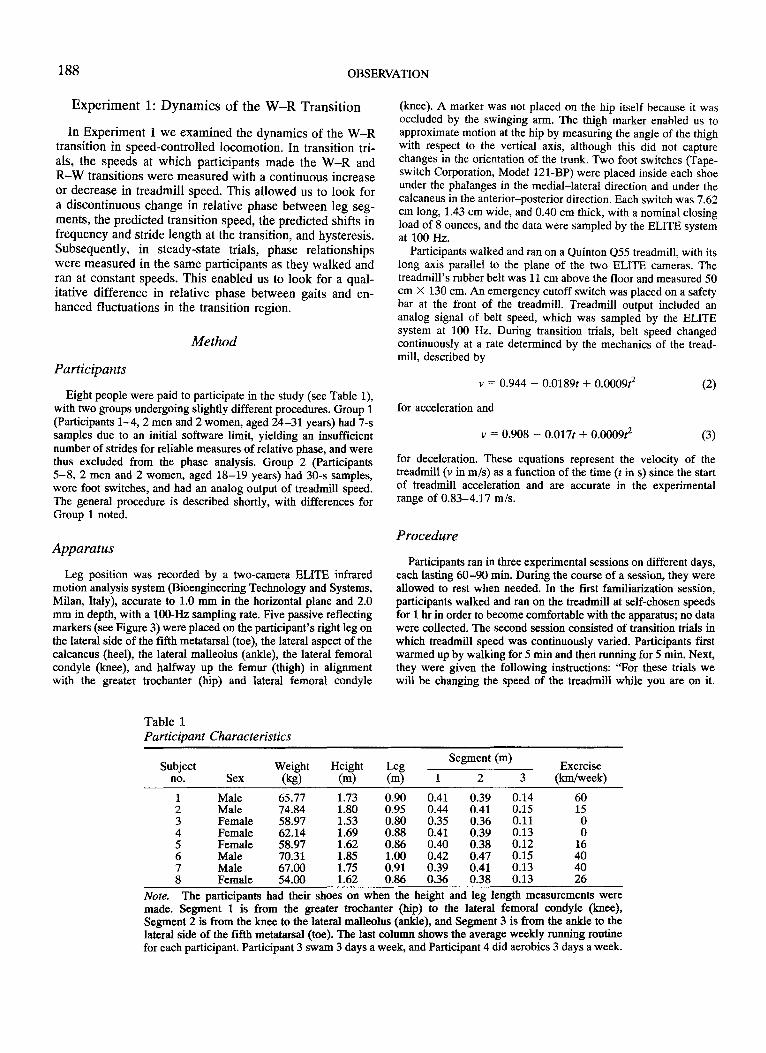
Eight people were paid to participate in the study (see Table 1), with two groups undergoing slightly different procedures. Group 1 (Participants 1-4,2 men and 2 women, aged 24-31 years) had 7-s samples due to an initial software limit, yielding an insufficient number of strides for reliable measures of relative phase, and were thus excluded from the phase analysis. Group 2 (Participants 5-8,2 men and 2 women, aged 18-19 years) had 30-s samples, wore foot switches, and had an analog output of treadmill speed. The general procedure is described shortly, with differences for Group 1 noted.

Apparatus

Leg position was recorded by a two-camera ELITE infrared motion analysis system (Bioengineering Technology and Systems, Milan, Italy), accurate to 1.0 mm in the horizontal plane and 2.0 mm in depth, with a 1OO-Hz sampling rate. Five passive reflecting markers (see Figure 3) were placed on the participant's right leg on the lateral side of the fifth metatarsal (toe), the lateral aspect of the calcaneus (heel), the lateral malleolus (ankle), the lateral femoral condyle (knee), and halfway up the femur (thigh) in alignment with the greater trochanter (hip) and lateral femoral condyle

Table 1 Participant Characteristics

Subject Weight Height no. Sex (kg) (m)

1 Male 65.77 1.73 2 Male 74.84 1.80 3 Female 58.97 1.53 4 Female 62.14 1.69 5 Female 58.97 1.62 6 Male 70.31 1.85 7 Male 67.00 1.75 8 Female 54.00 1.62

(knee). A marker was not placed on the hip itself because it was occluded by the swinging arm. The thigh marker enabled us to approximate motion at the hip by measuring the angle of the thigh with respect to the vertical axis, although this did not capture changes in the orientation of the trunk. Two foot switches (Tape­switch Corporation, Model 121-BP) were placed inside each shoe under the phalanges in the medial-lateral direction and under the calcaneus in the anterior-posterior direction. Each switch was 7.62 cm long, 1.43 cm wide, and 0.40 cm thick, with a nominal closing load of 8 ounces, and the data were sampled by the ELITE system at 100 Hz.

Participants walked and ran on a Quinton Q55 treadmill, with its long axis parallel to the plane of the two ELITE cameras. The treadmill's rubber belt was 11 cm above the floor and measured 50 cm X 130 cm. An emergency cutoff switch was placed on a safety bar at the front of the treadmill. Treadmill output included an analog signal of belt speed, which was sampled by the ELITE system at 100 Hz. During transition trials, belt speed changed continuously at a rate determined by the mechanics of the tread­mill, described by

v = 0.944 - 0.0189t + 0.Ooo9r (2)

for acceleration and

v = 0.908 - 0.017t + 0.OO09r (3)

for deceleration. These equations represent the velocity of the treadmill (v in m/s) as a function of the time (t in s) since the start of treadmill acceleration and are accurate in the experimental range of 0.83-4.17 m/s.

Procedure

Participants ran in three experimental sessions on different days, each lasting 60-90 min. During the course of a session, they were allowed to rest when needed. In the first familiarization session, participants walked and ran on the treadmill at self-chosen speeds for 1 hr in order to become comfortable with the apparatus; no data were collected. The second session consisted of transition trials in which treadmill speed was continuously varied. Participants first warmed up by walking for 5 min and then running for 5 min. Next, they were given the following instructions: "For these trials we will be changing the speed of the treadmill while you are on it.

Leg Segment (m)

Exercise (m) 1 2 3 (km/week)

0.90 0.41 0.39 0.14 60 0.95 0.44 0.41 0.15 15 0.80 0.35 0.36 0.11 0 0.88 0.41 0.39 0.13 0 0.86 0.40 0.38 0.12 16 l.OO 0.42 0.47 0.15 40 0.91 0.39 0.41 0.13 40 0.86 0.36 0.38 0.13 26

Note. The participants had their shoes on when the height and leg length measurements were made. Segment 1 is from the greater trochanter (hip) to the lateral femoral condyle (knee), Segment 2 is from the knee to the lateral malleolus (ankle), and Segment 3 is from the ankle to the lateral side of the fifth metatarsal (toe). The last column shows the average weekly running routine for each participant. Participant 3 swam 3 days a week, and Participant 4 did aerobics 3 days a week.

OBSERVATION 189

a 1

2

-- . 4 5

Figure 3. Marker placement and joint angles: 1 = thigh marker, 2 = knee marker, 3 = ankle marker, 4 = heel marker,S = toe marker; 0: = hip angle (to vertical), {3 = knee angle, 'Y = ankle angle.

Please walk or run as feels comfortable. That is, make the transi­tion when it seems natural to do so." Treadmill speed was alter­nately increased (W-R) and decreased (R-W), with half of the participants starting in a W-R trial and half in an R-W trial. There were 5 practice trials in each direction, followed by 15 test trials in each direction, and ELITE data collection windowed the transition speed. 1

The third session consisted of steady-state trials in which par­ticipants walked and ran at a set of constant speeds, which over­lapped for the two gaits. Participants repeated the warm-up se­quence and were then instructed to walk or run at a constant treadmill speed. Speed was equated across participants using the Froude number (F), a dimensionless parameter that normalizes speed with respect to leg length (see Equation 1). Participants were tested at Froude numbers of 0.1, 0.25, 0.4, 0.5, 0.6, and 0.7 for walking (0.9-2.5 m/s) and 0.25, 0.4, 0.5, 0.6, 0.7, 0.85, 1.0, 1.15, 1.3, and 1.45 for running (1.5-3.6 m/s)? Each participant received four blocks of trials in a counterbalanced order. Within a block, there was one trial at each of the speeds noted earlier, in an ascending or descending order for a given gait before proceeding to the other gait. A 30-s data sample was collected appro xi-

mately 10 s after the treadmill was adjusted to the proper speed. This conformed to the so-called "delay convention" for observing critical fluctuations (see Schmidt, Carello, & Turvey, 1990, for a discussion), according to which the time for recovery from per­turbation ('Trelaxation) must be markedly less than the plateau time for the control parameter ( 'T controJ, which in turn must be markedly less than the time to pass from one phase to another due to random fluctuations ( 'T passage). Recovery fr~m perturbation typically oc~s within one cycle (Kelso, Holt, Rubm, & Kugler, 1981; Orlovskii & Shik, 1965); plateau trials lasted approximately 40 s, and we never observed spontaneous phase transitions in our samples.

Data Analysis

Transition trials were analyzed to determine the speed, stride frequency, and stride length in the last complete stride cycle before the one containing the transition (pretransition) and the fIrst com­plete stride cycle after it (posttransition). Steady-state trials were analyzed to determine the mean frequency, stride length, and (for Group 2 only) relative phase for the entire trial and the within-trial standard deviations of these variables.

Basic gait parameters. The kinematic data were fIltered using a fourth-order Butterworth low pass fIlter with a ll.5-Hz cutoff, and joint angle time series were then computed. Knee and ankle angles were defmed as saggital projections of the angles between the thigh, shank, and foot segments, and the hip angle was defined as the sagittal projection of the angle between the thigh segment and the vertical axis (see Figure 3). The joint angle time series were then analyzed to determine the time of peak flexion and extension at each joint. A peak-picking program located a joint angle extremum and then searched forward and backward in time to fmd the fIrst point that was 10 below the extremum (the noise criterion). The peak was taken to occur at the time average of these two side points and usually coincided with the extremum.

For each stride, frequency was determined as the inverse of the period between an identifIable landmark in successive stance phases of the right leg, the midpoint between activation of the right heel and toe switches; the corresponding speed was taken from the treadmill output (averaged over fIve frames), and stride length was computed from these values (s = v/f). On transition trials, running was indicated by the presence of a flight phase with all foot switches open simultaneously, and the transition stride was iden­tifIed as the fust (W-R) or last (R-W) stride containing a flight phase. The pre- and posttransition speed, frequency, and stride length were then determined from the strides immediately prior to and following the transition stride. We refer to the pretransition values as "transition values." On steady-state trials, measurements of speed, frequency, and stride length were obtained from the first 17 complete stride cycles of each trial, so that equal numbers of cycles would contribute to within-trial standard deviations.3

Relative phase. In each steady-state trial, the relative phases of

1 Group 1 did not receive the familiarization session and per­formed only 10 test trials in each direction.

2 Group 1 was tested at slightly different speeds that were later converted to Froude numbers and binned to correspond with these values. A bin contained only one or two speeds for any individual.

3 Because Group 1 did not wear foot switches, stride frequency was determined from successive peak hip extensions, and the corresponding speed was determined from the horizontal speed of the toe marker during midstance on the treadmill (averaged over three frames). On transition trials, the transition stride was identi­fIed as the one in which the relative phase between peak ankle plantar flexion and peak knee extension during stance shifted

190 OBSERVATION

the hip, knee, and ankle angles at peak extension during toe-off were computed from the joint angle time series of the right leg. Specifically, peak ankle plantar flexion was compared with peak knee extension and peak hip extension. The time between succes­sive peak hip extensions (the reference cycle) was defined as 360°, and the relative phase of peak ankle plantar flexion (the target) was described as a proportion of this reference cycle in degrees. Anal­ogously, peak knee extension provided the reference cycle for peak ankle plantar flexion (see Figure 4). This point estimate of relative phase was appropriate because intersegmental timing is critical during force application culminating in toe-off, and because cor­responding landmarks in the time series could be reliably identi­fied. Such a point estimate is more reliable than a continuous relative phase estimate because it does not assume that the time series is sinusoidal or stationary. Preliminary analysis of peak flexion during stance revealed similar results.

The first 21 stride cycles in each steady-state trial were analyzed for mean relative phase and within-trial standard deviation. Be­cause phase is a circular (360°) variable, we calculated all means, standard deviations, and statistical tests of phase using the methods of circular statistics (Batschelet, 1981; Burgess-Limerick, Aber­nethy, & Neal, 1991; see also Appendix B). Out of the 256 steady-state trials collected, occlusion of markers or equipment malfunction resulted in 19 missing trials. A participant's score for a condition with a missing trial was the average of his or her other trials in that condition.

Results

Transition Trials

Sudden jump. Transitions were marked by a sudden jump in relative phase that occurred within one stride cycle, as illustrated by a typical trial in Figure 5. Inspection of the ankle-knee phase relationships for the first 10 W-R and R-W transitions of each participant showed that this was the case on every trial, with mean W-R jumps from 75.11° to 23.01°, t(7) = 12.28, p < .001, and mean R-W jumps from 25.70° to 73.68°, t(7) = 13.21, P < .001. There was close agreement between the appearance of a flight phase in the foot switch data and the shift in relative phase on these trials, validating relative phase as an index of the gait transition.

Transition speed, frequency, and stride length. Transi­tion variables for each participant appear in Table 2, and means are plotted in Figure 6. The mean pretransition speed over both W-R and R-W directions was 2.07 mls (SD = 0.21 mis, F = 0.49, SD = 0.08), lying right on the energy separatrix. At the W-R transition (open circles in Figure 6), participants jumped from their preferred walking path ( dashed line) to the running trough, whereas at the R-W transition (filled circles), they jumped back. Mean frequency rose by 0.06 Hz and stride length fell by 2 cm at

between values characteristic of walking and running (see Figure 7). Because of missed transitions that occurred outside the 7-s acquisition window, only the first 7 of 10 transition trials in each direction were analyzed for each participant. On steady-state trials, speed, frequency, and stride length were determined from the first four complete stride cycles, but we did not compute within-trial standard deviations because of this small number of strides.

A 250.0 t Flexion

200.0

Oi 1.\0.0 Q)

:£. Q) 100.0 c;, c: « "E 5l.0 '0 '"')

0.0

0.0 OJ 1.0 U 2.0 15 3.0 15 Time(s}

B :00.0

1~.0

100.0

lO.O

0.0 OJ 1.0 IJ !oO 2..1 1.0 1.5

Time (s)

Figure 4. Sample trials from Participant 8 showing joint angles as a function of time during (A) walking and (B) running. Relative phase is calculated by defining A to A' as the 360° reference cycle, and defining Event B as a proportion of this cycle.

the W-R transition; conversely, frequency fell by 0.08 Hz and stride length rose by 4 cm at the R-W transition, all in the expected direction. Although these shifts were small, the chance probability of all four of them being in the expected direction was only 1/16, (p = .062). Combining W-R and R-W values, the running frequency at the transition (1.24 Hz, SD = 0.06 Hz) was significantly higher than the walk­ing frequency (1.17 Hz, SD = 0.07 Hz), as predicted, paired t(7) = 2.57, p < .05. The running stride length at the transition (1.71 m, SD = 0.21 m) tended to be lower than that for walking (1.74 m, SD = 0.14 m), although this was not significant, t(7) = 0.80, ns. In general, these data are consistent with the dynamic theory.

Hysteresis. The mean W-R pretransition speed of 2.09 mls (F = 0.50, SD = 0.10) was slightly higher than the mean R-W pretransition speed of 2.05 mls (F = 0.48, SD = 0.07; see Table 2), suggesting the presence of hys-

OBSERVATION

100 ..... ~... ,

...... , Ie

80 Flight-Phase Present

Ci 60 Q)

:8. Q) CIJ ro 40 .!: a.. Q)

> ·ia 20 Q)

II:

0

-20 14 16 18 20 22 24 26

Time (s)

Figure 5. The relative phases of the leg segments during a sample walk-run transition trial. The vertical line indicates onset of flight phase (participant 7); deg = degrees.

191

teresis. A two-way analysis of variance (ANOV A) on tran- a significant interaction, F(7, 74) = 8_12, P < .01, that sition speed (Froude number), with degrees of freedom revealed individual differences in the amount and direction adjusted for unequal numbers of trials, confirmed this ef- of hysteresis. Analyses of simple effects indicated that Par-fect, F(l, 74) == 10.02, p < .01, as well as individual dif- ticipants 1, 2, and 5 showed significant hysteresis in the ferences in transition speed, F(7, 74) == 77.95, p < .01, and expected direction (p < .05), Participants 4 and 7 showed

Table 2 Transition Statistics for Individual Participants

Subject Velocity (Froude) Velocity (m/s) Stride frequency (Hz) Stride length (m)

no. Type Pre Post Pre Post Pre Post Pre Post

1 W-R 0.58 0.62 2.26 2.34 1.19 1.26 1.90 1.86 R-W 0.51 0.49 2.13 2.08 1.23 1.13 1.74 1.84

2 W-R 0.66 0.66 2.47 2.48 1.29 1.26 1.92 1.97 R-W 0.55 0.55 2.26 2.26 1.25 1.22 1.82 1.86

3 W-R 0.41 0.43 1.80 1.84 1.12 1.24 1.61 1.48 R-W 0.44 0.41 1.85 1.79 1.18 1.16 1.57 1.55

4 W-R 0.38 OAO 1.82 1.87 1.09 1.32 1.68 1.41 R-W 0.37 0.34 1.80 1.70 1.24 1.06 1.45 1.60

5 W-R 0.44 OA8 1.92 2.00 1.20 1.33 1.60 1.50 R-W 0.40 0.37 1.84 1.77 1.29 1.16 1.43 1.53

6 W-R 0.44 0.48 2.07 2.17 1.10 1.09 1.88 1.98 R-W 0.50 0.44 2.22 2.09 1.16 1.08 1.91 1.94

7 W-R 0.56 0.62 2.24 2.36 1.26 1.19 1.78 1.98 R-W 0.50 OA5 2.11 2.00 1.19 1.16 1.77 1.73

8 W-R 0.56 0.61 2.16 2.27 1.26 1.29 1.72 1.76 R-W 0.56 0.51 2.18 2.07 1.31 1.28 1.67 1.62

M W-R 0.50 0.54 2.09 2.17 1.19 1.25 1.76 1.74 R-W 0.48 0.44 2.05 1.97 1.23 1.15 1.67 1.71

SD W-R 0.10 0.10 0.23 0.24 0.08 0.08 0.13 0.24 R-W 0.07 0.07 0.19 0.19 0.05 0.07 0.17 0.16

Note. Pre = pretransition; Post = posttransition; W-R = walk-run transition; R-W = run-walk transition.

192 OBSERVATION

2.5

2.0

E '-' 1.5 -.0 .;(1<

(J)

1.0

05 03 05 07 09 11 13 15

f (Hz)

Figure 6. Mean stride length and frequency data superimposed on the energetic contour plot. Dashed lines indicate mean preferred stride length (s)/stride frequency if) combinations in Exper­iment 1, open circles indicate mean pre- and posttransition values for the walk-run transition in Experiment 1, filled circles indicate these values for the run-walk transition, and triangles indicate mean pretransition values in Experiment 2.

trends in the expected direction (ns), Participants 3 and 8 had trends in the opposite direction (ns), and Participant 6 had a significant effect in the opposite direction (p < .05).

Steady-State Trials

Relative phase. Mean relative phase data for Group 2 are reported in Figure 7 and Table 3. In general, during toe-off the ankle appeared to be out of phase with both the knee and hip in walking, but nearly in-phase in running. First, during walking the hip fully extended before the ankle reached peak plantar flexion, but these two events occurred almost simultaneously in running. Watson-Williams F tests for circular variables showed significant differences in phase between the gaits for each participant: Participant 5, F(1, 14) = 57.38,p < .01; Participant 6, F(1, 14) = 850.78, p < .01; Participant 7, F(l, 14) = 588.10, p < .01; and Participant 8, F(l, 14) = 132.90, p < .01. Second, peak extension of the knee also occurred before peak plantar flexion of the ankle when walking, but these events oc-

curred more in-phase during running: Participant 5, F(l, 14) = 87.36, p < .01; Participant 6, F(l, 14) = 729.93, p < .01; Participant 7, F(1, 14) = 1380.52, p < .01; and Participant 8, F(1, 14) = 359.46, p < .01. This demon­strates a qualitative reorganization in the phasing of limb segments between gaits.

It is also worth noting that the relative phase within each gait tended to drift slightly as a function of speed. Recent experiments on interlimb coordination between arms and legs have shown that when people were instructed to in­crease frequency, a similar slow drift in relative phase between limbs of different length and mass was observed (Kelso & Jeka, 1992), presumably due to differences in the natural frequencies of the limbs. The segments of the leg (thigh, calf, and foot) in this study were also of different length and mass, and thus the drift in relative phase could have been due to the different natural frequencies of these segments.

Enhanced fluctuations. In general, fluctuations in rela­tive phase tended to increase near the transition, as indicated

OBSERVATION 193

A 60

C; Q)

:!:!. Q) rn aI .c c.. Q) > ~ Q) a:

B

C; Q)

:!:!. Q)

gj .c c.. Q) > ~ Q) a:

40

20

0

-20 0.0

100

80

60

40

20

0

~

" \ \ \ \ \

Q \ , \ ,\

"

~.(: ,

0.0

-- walkS

t-.. --I!t- runS - walk 6 ..,... ., --.- run6 - walk 7 --It- run 7 --0-- walkS --0'- runS

'0.

\ .... ,0. \ ,

' .... , \

Ia. .... 00_-00 -_00

__ 0

, "', ',. "', ',.. .. ·~J:~·;~tc~~.=.=;a

&--EI'"

0.5 1.0 1.5 2.0

Froude Number

-- walk 5 --e- run 5 - walk 6 --,.- run 6 - walk 7 --It- run 7 --0-- walk S --0- runS

0.5 1.0 1.5 2.0

Froude Number

Figure 7. Mean relative phase for each participant during walk­ing and running as a function of speed showing (A) data for ankle and hip and (B) data for ankle and knee. Vertical lines indicate the transition region, ± 1 SD from the mean transition speed. These data are from the steady-state trials of Group 2.

by the within-trial standard deviations of phase. During walking, the standard deviation of ankle-hip phase was a U-shaped function of speed (see Figure 8A), with an in­crease in variability in the transition region and at low speeds, F(5, 15) = 7.09, p < .001. Single degree-of-free­dom polynomial contrasts indicated a significant quadratic component, F(l, 3) = 17.28, p < .05, and the least squares regression equation describing the walking curve was as follows: SD = 4.15 - (8.78 F) + (11.52 F2), r2 = .98, with a minimum at F = 0.38 (1.83 m/s). In running, the ankle­hip standard deviation also increased in the transition re­gion, F(9, 27) = 18.50, p < .001, but flattened out at higher speeds. There was a significant quadratic component, F(l, 3) = 19.89, p < .05, and the regression equation was as

follows: SD = 11.24 - (13.93 F) + (6.38 F2), r2 = .90. All 4 participants exhibited this pattem.4

For the ankle-knee relation (see Figure 8B), the standard deviation of relative phase also exhibited a V-shaped func­tion during walking, F(5, 15) = 13.39, p < .001, with a significant quadratic component, F(l, 3) = 18.38, p < .05. The equation for the curve was as follows: SD = 9.38 -(28.61 F) + (32.21 F2), r2 = .89, with a minimum at the comparatively high speed of F = 0.44 (1.97 m/s). In con­trast to the ankle-hip relationship, this minimum appeared in the transition region, and the standard deviation began to increase only at speeds above the transition region. This inconsistency was due primarily to 2 participants who had low standard deviations in the transition region. In the running gait, however, the ankle-knee standard deviation once again increased near the transition region, F(9, 27) = 11.39, p < .01, and flattened out at higher speeds, with no significant quadratic component, F(l, 3) = 6.64, ns.

Although the evidence for enhanced fluctuations in the R-W transition was strong, that for the W-R transition was weaker: The standard deviation of phase exhibited only small increases in the transition region. This could have been due to our method in the steady-state trials. Previous procedures have let participants make the transition, thus allowing for the alignment of pretransition plateaus in the computation of mean standard deviations. By estimating the mean transition speed in a separate session, we inevitably combined some plateaus from pre- and posUransition speeds, diminishing the rise in the standard deviation. De­spite one inconsistent result, overall we take these data as evidence for an increase in fluctuations of relative phase in the transition region.

Mean stride frequency and stride length. The mean s/f combinations in steady-state trials are ploUed as dashed lines in Figure 6 and indicate the preferred route to the transition. Our participants were close to the optimal line for walking and the trough for running predicted from the energetic data. In general, mean frequency and stride length increased with speed for both gaits (see Figure 9), as pre­viously reported. This was the case for walking, which showed a significant effect of speed on frequency­Group 1, F(4, 12) = 46.17, p < .001; Group 2, F(5, 15) = 323.06, p < .OOl-and on stride length-Group 1, F(4, 12) = 30.23, p < .001; Group 2, F(5, 15) = 150.72, p < .001. It was also the case for running, with a significant effect of speed on frequency-Group 1, F(4, 12) = 9.73, p < .01; Group 2, F(9, 27) = 8.32, p < .00l-and stride length-Group 1, F(4, 12) = 149.55, p < .001; Group 2, F(9, 27) = 92.78, p < .001. The effect of speed on fre­quency was much greater in walking than in running, wherein the preferred frequency changed little.

4 Note that comparisons of variability cannot be made between gaits because peaks of ankle plantar flexion were more rounded in running than walking, increasing the inherent variability in the peak-picking algorithm. This may account for the higher standard d~viations in running compared with walking that are apparent in FIgure 8. Thus, the speed at which the curves intersected has no particular significance.

194 OBSERVATION

Table 3 Relative Phases

Ankle-hip Ankle-knee Subject no. and statistic Walk (degrees) Run (degrees) Walk (degrees) Run (degrees) 5

M SD

44.99 -4.72 77.89 18.72 2.86 14.93 9.45 12.49

6 M SD

47.26 -11.77 82.08 8.28 4.02 3.47 6.62 3.56

7 M SD

44.34 -10.81 83.37 8.85

8 M SD Grand

3.68 4.41

44.23 2.94 0.72 8.29

5.34 1.83

81.42 20.91 1.68 7.23

M SD

45.20 -6.12 81.20 14.19 2.36 5.92 1.21 5.51

Note. Each participant's score is the average across all speeds tested in a given gait.

Maruyama and Nagasaki (1992) recently reported that during forced walking, in which both speed and frequency were specified, the standard deviation of the step period (the inverse of frequency) increased at low speeds, suggesting a loss of stability. To examine the stability of frequency and stride length near the transition, we plotted their standard deviations as a function of speed in Figure 10 (Group 2 only). During walking, variability in frequency increased at low speeds and again near the transition, F(S, IS) = 2.82, P < .OS4, although the quadratic component was not sig­nificant, F(I, 3) = 7.27, ns. A similar trend for the standard deviation of stride length was not significant, F(S, IS) = 2.57, ns. For running, there were no significant ef­fects of speed on the standard deviation of frequency, F(9, 27) = 1.784, ns or on the standard deviation of stride length, F(9, 27) = 0.96, ns. Thus, variability in relative phase appears to be a more sensitive measure of stability than variability in frequency or stride length.

This pattern of results bears out the dynamic theory. Assuming speed as a control parameter and relative phase as an order parameter, we predicted that continuous variation in speed would yield a gait transition near the energy separatrix, specific shifts in stride length and frequency, a qualitative reorganization of limb phasing, a sudde? jump in relative phase, hysteresis, and enhanced fluctuatIons. The data are consistent with these predictions. Clearly, there is a preferred phase as well as a preferred stride l~ngth and frequency in each gait, indicative of an attractor III phase­frequency-stride length space. Similarly, the U-shaped fluc­tuation curves suggest attractors with maximum stability at a particular speed (stride length and frequency combina­tion), although this is evaluated more fully in the General Discussion.

Experiment 2: Forced Gait Transitions

Although the W-R transition occurred at a speed corre­sponding to the energy separatrix, Experiment 1 was an

observational study and it remains possible that some other correlated factor elicited the shift. Participants crossed the separatrix at only one point, the preferred s/f ratio. Experi­ment 2 provided an experimental test by forcing participants across the separatrix at several nonpreferred points. We did this by using a forced gait, artificially increasing or decreas­ing stride frequency at a given treadmill speed by asking participants to keep pace with a metronome. Assuming that total energy expenditure approximately reflects the under­lying dynamics, the theory predicts that a transition should occur when the s/f combination is near the 1.0 cal/kglm separatrix. In the region around the optimal crossing point (see Figure 6), the separatrix is close to an iso-speed contour of about 2.1 m/s. Thus, we would expect the transition to occur at a constant speed around 2.1 m/s despite variation in the pacing frequency.

This manipulation also allowed us to evaluate the control parameter for gait. Candidate control parameters that take the system through a gait transition include frequency, stride length, and their combination, speed. Although these variables were confounded in the preferred gait of Experi­ment 1, the present experiment dissociates them with a forced gait. If frequency is the relevant control parameter, then as pacing frequency is increased, we might expect the transition to occur at a constant critical frequency, yielding decreases in both the transition speed and stride length. Conversely, if stride length is the primary control parame­ter the transition should occur at a constant critical stride ledgth, yielding increases in both the transition frequency and speed with increases in pacing frequency. Finally, in a two-parameter system with a transition at the separatrix, we would expect the transition to occur at a constant speed, yielding an increase in the transition frequency and a de­crease in the transition stride length with increases in pacing frequency. Given the preferred coupling between frequency and stride length, we could then treat speed as a control parameter.

OBSERVATION 195

A

Ci Q)

~ Q)

!Q .c a. '5 0 C/)

!ij Q)

::=

B

10

8

6

4

2 0.0

l\ -- walk

--.-- run , \ ,

I I I , ,

l- -i 1 ~

~ .... 'f--r .... ,"

~ ~

10~----r-,-------------------,

8

6

4

2+-~ __ ~L-__ --~ __ ---r--__ ~

0.0 0.5 1.0 1.5 2.0

Froude Number

Figure 8. Mean within-trial standard deviation of relative phase during walking and running as a function of speed showing data for (A) ankle and hip and (B) ankle and knee. Vertical lines indicate the transition region and error bars indicate standard error. These data are from the steady-state trials of Group 2. SD = standard deviation; deg = degrees.

Method

Participants

Six people (3 men and 3 women) were paid to participate; 5 of these individuals had participated in Experiment 1 (participants 1 and 5-8). The one new participant was a female professional dancer, aged 24 years, 1.52 m tall, and 47.6 kg.

Apparatus

Leg movements during treadmill running were recorded by the ELITE motion analysis system and footfalls were recorded by foot switches. Stride frequency was manipulated by instructing partic­ipants to keep pace with 17-ms beeps generated on a Macintosh microcomputer and amplified through a Panasonic Model RX-

5030 radio. Initial "synchronization" beeps were low-pitched 750-Hz tones, whereas "test" beeps were high-pitched 900-Hz tones. The occurrence of each beep was recorded by the ELITE system at a sampling rate of 100 Hz.

The beeps occurred at the step frequency, one for each left and right footfall. During each trial the beep rate changed with the speed of the treadmill in order to keep frequency dissociated from speed. The beep rate increased or decreased in a manner dete.r­mined by the following procedure: (a) The speed of the treadmill was calculated from the time since the start of acceleration or deceleration (Equations 2 and 3) and was then converted to a Froude number (see Equation 1). (b) The preferred frequency was estimated from the Froude number on the basis of linear regression equations from Group 1 in Experiment 1 for the limited range of speeds tested:

f = 0.719 + (1.018F) (4)

~ walkS --Ilt- runS - walk 6 --~- run 6 - walk 7 --)f- run 7 --0-- walk 8 --0- run 8

o. 7 +--....--'--,..L--~-T--~-r---~--I 0.0 0.5 1.0 1.5 2.0

B Froude Number

3.0..----....---.-----------,r----, , , , /~ , ...

, ,It ",' , , , ~ "" , , ,

~"" ,)t '" , , 4!f~~a , It , ~ ,

" , , , ,<1 .rz'

" ,'" ~ walkS , --Ilt- runS

2.5

I .c Cl c: 2.0 Q) -.I Q)

"C - walk 6

--~- run 6 - walk 7

·c Ci5

1.5 --)f- run 7 --0-- walk 8 --0- run 8

1.0 +---~...L....,...l.-~---r---~--..___---.---1 0.0 0.5 1.0 1.5 2.0

Froude Number

Figure 9. (A) The mean stride frequency as a function of speed for each participant. (B) The mean stride length as a function of speed for each participant. Vertical lines indicate the transition region. These data are from the steady-state trials of Group 2.

196 OBSERVATION

N ~ () c:: Q) :;, 0-~

u.. Q) "0 .~

U5 '0 0 C/)

c:: til Q)

~

E ..c:: 0, c:: Q)

...J Q) "0 .~

U5 '0 0 C/)

c:: til Q)

~

0.032

0.028

0.024

0.020

0.016

0.012

0.008 0.0

0.045

0.040

0.035

0.030

0.025

0.020

0.015 0.0

-- walk --.-- run

\ \\ \

~ --H-t-t-i \

~

~ ~

0.5 1.0 1.5 2.0

Froude Number

-- walk --.-- run

1\ .... r, -t-H/H \V 17'

...... V

0.5 1.0 1.5 2.0

Froude Number

Figure 10. (A) The mean within-trial standard deviation of stride frequency. (B) The mean within-trial standard deviation of stride length. Vertical lines indicate the transition region and error bars indicate standard error. These data are from the steady-state trials of Group 2. SD = standard deviation.

for walking (r = .97) and

f = 1.222 + (0.127F) (5)

for running (r = .60). (c) Finally, the pacing frequency was de­termined by manipulating the y-intercepts of Equations 4 and 5 to obtain a percentage of change relative to the preferred frequency. An increase in the y-intercept produced a higher than preferred pacing frequency (+%) and, consequently, a lower than preferred stride length for any given treadmill speed. Conversely, a decrease in the y-intercept produced a lower than preferred pacing fre­quency (-%) and a higher than preferred stride length. For W-R trials, each participant was tested at five pacing frequencies, with changes of -15%, -10%, 0%, +10%, and +20% from the esti­mated preferred frequency. For R-W trials, they were tested at -20%, -10%, 0%, +10%, and +15% pacing frequencies.

These values were chosen in order to vary frequency as much as possible within the limits of each gait.

Procedure

Participants performed this experiment over two sessions, each lasting approximately 90 min. They were allowed to rest when needed. At the beginning of each session, participants warmed up by walking for 5 min and then running for 5 min at self-chosen speeds. They were then given the following instructions: "For these trials, we will be changing the speed of the treadmill while you are on it. Your job is to stay in synchrony with the beeps; that is, your feet should make contact with the ground when the computer beeps. In addition, please walk or run as feels comfort­able. That is, make the transition at that speed that seems natural to do so." Trials began at a speed of 1.17 mls for the W-R direction and at 3.00 mls for the R-W direction. Each trial started with 10 low synchronization beeps at a constant rate and a constant treadmill speed, during which time the participant synchronized to the beeps. When the treadmill began to accelerate or decelerate, high test beeps were presented at a rate determined by the method described earlier. The beeps ended when the transition was made so the participant could shift to a preferred gait pattern, leaving the competing attractor undisturbed by the pacing frequency. The next trial began approximately 5 s after completion of the previous trial, in the opposite direction. A trial was 30 s in duration. In each session, participants were given 5 practice trials in the 0% W-R and 5 in the 0% R-W conditions. They then performed each condition five times, for a total of 10 trials in each condition over the two sessions. W-R trials alternated with R-W trials and were counterbalanced across participants. The order of pacing frequency conditions was randomly determined for each participant.

The pretransition speed, stride length, and stride frequency were calculated for each trial as in Experiment 1, and W-R and R-W trials were combined. Note that the data from the most extreme pacing frequencies in each direction were averaged together, com­bining W-R trials at -15% with R-W trials at -20% (yield­ing -17.5%), and combining W-R trials at +20% with R-W trials at +15% (yielding +17.5%).

Results

Mean pretransition values as a function of percentage of change in pacing frequency appear in Figure 11 and were analyzed with one-way repeated measures ANDV As. As the pacing frequency was increased, the transition stride fre­quency increased significantly, F(4, 20) = 51.99, p < .001 (accounting for 91 % of the total sum of squares), and the transition stride length decreased significantly, F(4, 20) = 14.28,p < .001 (75% of the total sum of the squares). However, the transition speed did not change significantly, F(4, 20) = 0.41, ns (8% of the total sum of the squares), but remained approximately constant at 2.20 m/s (F = 0.55) with a between-conditions standard deviation of 0.02 m/s. This was precisely the pattern of results expected if the transition was made at the separatrix, with speed as the control parameter.

As a converging measure, we calculated the change in these transition values as a proportion of the total range of variation observed in the steady-state trials of Experiment 1. In those trials, speed was varied from 0.95 to 3.58 m/s,

OBSERVATION 197

A 2.30

2.25 (i) '-.s

2.20 "0 Q) Q) a. (/)

2.15

2.10 -17.5 -10 0 +10 +17.5 Percent Change in Pacing Frequency

B 1.35

N 1.30 ~ ~ 1.25 c:: Q) :::I 1.20 C" Q) --u.. 1.15 Q) "0 .t:

1.10 -(/) 1.05

-17.5 -10 0 +10 +17.5 Percent Change in Pacing Frequency

C 2.1

I 2.0

..c:: 1.9 -C) c:: Q) -I

1.8 Q) "0 .t: -(/) 1.7

-1 7.5 -1 0 0 + 1 0 + 17.5 Percent Change in Pacing Frequency

Figure 11. (A) Mean transition speed, (B) frequency, and (C) stride length as a function of the percentage of change in pacing frequency from the estimated preferred frequency. Error bars in­dicate the standard error.

yielding a mean frequency range of 0.56 Hz, a mean stride length range of 1.45 m, and a mean speed range of 2.63 mls (see Figure 9). In Experiment 2, as pacing frequency was increased, the mean transition frequency increased by 0.18 Hz, a proportional change of 31 %, and the mean transition stride length decreased by 0.26 m, a proportional change of 18%, but the mean transition speed increased by 0.02 mis,

a proportional change of only 1%. These data again indicate that the transition speed was relatively constant when ex­pressed as a proportion of the normal range of variation, whereas the transition stride length and frequency varied considerably in the expected directions.

In summary, when participants were forced to used dif­ferent slj combinations, they made the transition at a con­stant speed of 2.20 mls rather than at a critical value of stride frequency or stride length. This was predicted by the theory that the transition occurs near the energy separatrix, for the separatrix is close to a constant speed of 2.1 mls in the transition region. The fact that the observed value was slightly higher than the predicted value and higher than the transition speed of 2.07 mls found in Experiment 1 might have been due to the forced gait requiring continual adjust­ments in stride frequency. We do not believe that a theory based on peak ground reaction force can account for this constant transition speed. Presumably, peak force would increase with stride length, triggering the transition at lower speeds with lower pacing frequencies.

The results are also consistent with the notion that the control parameter for the W-R transition is neither fre­quency nor stride length alone but their combination, which is conveniently expressed by speed in a preferred gait.

General Discussion

Why do humans and other animals change gaits? The results of this research support a dynamic theory of gait transitions, according to which each preferred gait behaves like an attractor characterized by stable phase relationships and minimum energy expenditure, and the gait shift behaves like a nonequilibrium p'hase transition between attractors that acts to reduce energy expenditure. This theory makes two somewhat independent claims: that gait transitions ex­hibit the qualitative behavior of phase transitions and that aspects of gait transitions correspond with the energetics. We discuss each in tum.

Energetics of the W-R Transition

Consider first the energetic claim. We propose that gait transitions are governed by a potential landscape that, along with other metabolic factors, is reflected in total energy expenditure. This loose correspondence allowed us to pre­dict successfully the transition speed and the pattern of stride length and frequency changes on the basis of previous energetic data (see Figure 6). Specifically, previous data indicated that the transition should occur at a speed of 2.1 mls to minimize energetic costs. The mean transition speed of 2.07 mls in Experiment 1 was right at this value, agreeing closely with Beuter and Lalonde's (1989) mean of 2.05 mls and Hreljac's (1993) mean of 2.07 m/s. When we forced participants away from the preferred slj combination in Experiment 2, the transition values remained close to the energy separatrix at a speed of 2.20 m/s. Furthermore, the energetics predicted a rise in frequency and a drop in stride length at the W-R transition and the reverse at the R-W

198 OBSERVATION

transition. Precisely this pattern was observed, with a sig­nificantly higher frequency in running than in walking, and a nonsignificant trend toward a shorter stride length in running than in walking. These results are consistent with the view that the system's critical behavior is closely related to the competition between attractors inferred from the energetics.

This distinction between dynamics and energetics might also account for the discrepancy between the preferred and energetically optimal transition speeds reported by Hreljac (1993) while allowing for the generally close relationship observed between preferred behavior and minimum ener­getic cost. It is possible that other factors can influence total energy expenditure without affecting, for example, the sensed cost of driving the legs in a particular gait. This could also account for Hreljac's puzzling finding that al­though energy expenditure at the transition speed was 16% higher for running than for walking, the rating of perceived exertion was 26% lower. Perceived exertion could be more closely related to the dynamics of a task than to the overall energetics. However, it would be desirable to model or measure the potential landscape independently.

Dynamics of the W-R Transition

Next consider the claim that gait transitions behave qual­itatively like nonequilibrium phase transitions. This would be informative even if one could not predict particular transition values. As expected, the W-R transition exhibited four hallmarks of a phase transition. First, there was a qualitative reorganization in the phasing of segments within a leg at the transition. At toe-off, extension occurred at the knee and the hip prior to the ankle in walking (out-of­phase)? whereas these joints extended almost synchronously in running (in-phase). Preliminary analysis of peak flexion during stance showed a similar phase difference between the gaits. These data are consistent with an inverted pendu­lum model of walking, in which the body passes over the stance leg, extending the knee and hip prior to final push-off at the ankle. The bouncing model of running, by contrast, implies an in-phase motion during stance, with simulta­neous flexion during weight acceptance followed by simul­taneous extension to capitalize on the elastic rebound of the leg and propel the body into the flight phase. This pattern, with a unique preferred phase for walking and for running, is suggestive of a point attractor in the phase variable for each gait.

Second, this qualitative shift in relative phase occurred in a sudden jump within a single stride cycle. A continuous change in a nonspecific control parameter (speed) thus yielded a discontinuous change in the order parameter (phase), with no intermediate states being occupied.

Third, the hysteresis effect was statistically significant, despite individual differences. Three participants showed significant hysteresis, 2 had a hysteresis trend, 2 had trends in the opposite direction, and 1 showed significant reverse hysteresis. Beuter and Lalonde (1989) previously demon­strated significant hysteresis, with a mean W-R transition

speed of 2.17 mls and a R-W speed of 1.93 m/s. They used a slightly different method with treadmill speed increasing stepwise with 15-s plateaus, rather than continuously, which could explain their stronger result. In summary, we believe that there is a small but real hysteresis effect in speed for the W-R transition.

Fourth, there was an increase in fluctuations of relative phase near the transition region for both walking and run­ning. The standard deviation of ankle-hip phase increased in the transition region for both gaits (see Figure 8A). The standard deviation of ankle- knee phase increased in the transition region for running but did so only for walking after the transition region (see Figure 8B). As mentioned earlier, this could have been due to our method of holding participants in the first mode past the normal transition point, so that the data could not be aligned at the transition for averaging. For the same reason, our data do not exhibit the sharp peak in variability at the transition seen in some previous studies of bimanual coordination that allowed sub­jects to make the transition (e.g., Kelso et aI., 1986). This sharp peak actually confounded two sources of variability, including both fluctuations due to the loss of stability (which one wants to measure) and larger fluctuations due to transitions to the second mode. If the transitional data point is removed, then their fluctuation curves look similar to ours. Overall, we take the results as evidence that variability in relative phase increased in the gait transition region. This indicates a loss of stability near the transition, as expected when two basins of attraction merge to define a broader set of probable states (see Figure 1).

The fluctuation data are also suggestive regarding attrac­tor states in the speed variable for each gait. For walking, the standard deviation curves were significantly U shaped as a function of speed, consistent with a stable attractor at the minimum. The minima-1.83 mls (ankle-hip) and 1.97 mls (ankle-knee }-were different from each other and higher than the preferred and optimal speed of 1.3 m/s. However, given our interest in the transition region, we did not sample enough lower speeds to reliably estimate these minima. We are currently testing a wider range of walking speeds to accurately determine the most stable speed. By contrast, the fluctuation curves for running were not U shaped: They dropped from high variability in the tran­sition region and flattened out at higher speeds. This is consistent with a valley of attraction for running in stride length-frequency space, with participants staying in the attractor trough at higher speeds. However, given our focus on the transition, we did not test speeds above 3.6 mis, and it is possible that variability would increase again at higher speeds.

Finally, the results of Experiment 2 are consistent with a two-parameter control space for gait (Figure 6). When we dissociated stride length, stride frequency, and speed, the transition was made at significantly different values of stride length and frequency, but near the separatrix at a constant value of speed. Thus, a control parameter of either stride length or frequency alone is insufficient. Because of the coupling of stride length and frequency in free locomo­tion, these variables are effectively expressed by a single

OBSERVATION 199

speed parameter, which can serve as a control parameter under natural conditions.

In summary, gait shifts appear to exhibit the hallmarks of a nonequilibrium phase transition. (We plan additional ex­periments examining critical slowing down in the transition region, a definitive characteristic of phase transitions.) This suggests that the locomotor system is governed by dynamics common to other complex physical systems, organized around attractors and bifurcations. By contrast, the view that gait transitions result from switching between central motor plans does not make such detailed predictions. We argue that the dynamic view thus provides a more adequate theory.

These results must be tempered by the fact that our research was conducted on a treadmill, as was that of Beuter and Lalonde (1989) and Hreljac (1993). In general, there is little evidence for significant differences in kinematics, electromyographic patterns, or energy expenditure between treadmill and overground locomotion in humans, with the exception of slightly lower variability on the treadmill (Arsenault, Winter, & Marteniuk, 1986; van Ingen Schenau, 1980). Studies of running have shown little or no difference in oxygen consumption, stride frequency, stride length, stance time, or swing time for the speeds tested in our experiments, although differences have emerged at higher speeds (Elliot & Blanksby, 1976; Nelson, Dillman, Lagasse, & Bickett, 1972; Pugh, 1970). Thus, treadmill and over­ground gaits are generally similar in the range tested, although overground experiments would certainly be desirable.

Modeling the Dynamics

Ultimately, we would like to develop a physical model of the dynamics that would describe the underlying potential function and even account for its relationship with the energetics. One possibility is Kugler and Turvey's (1987) hybrid mass-spring/pendulum model, which has been used to account for preferred frequencies of rhythmic movement. Applied to gait, this linear model treats the swing leg as a simple pendulum that is acted on by two components: a spring that represents the elastic properties of tendons and muscles at the hip joint and a forcing function that repre­sents active muscle contraction (Turvey, Schmidt, Rosen­blum, & Kugler, 1988). Each gait is assumed to have a characteristic hip stiffness, yielding a natural frequency that requires minimum driving force (minimum cost) to main­tain a given amplitude of oscillation, thus providing a de­scription of the potential landscape. The model has been used to fit preferred frequencies of walking and running, with stiffness as a free parameter (Holt, Hamill, & Andres, 1990, 1991; Holt, Slavin, & Hamill, 1990; Turvey et aI., 1988; see also Hatsopoulos & Warren, 1993).

Accepting the empirical stiffness values and assuming that stride length and frequency are the same in each gait at the transition, we used equations from previous articles (Turvey et aI., 1988; Holt, Hamill, & Andres, 1990) to derive an expression that predicts the transition frequency

(at which the driving force is equal in the two gaits):

w = [(w~alk + w~run)/2J1/2 (6)

For each participant in Experiment 1, we used Dempster's (1955) equations to estimate segment centers of mass, de­termined the simple pendulum equivalent of the leg and the natural frequency of each gait (see Holt, Hamill, & Andres, 1990; Holt, Slavin, & Hamill, 1990), and calculated the transition frequency from Equation 6. The mean predicted transition frequency of 1.23 Hz (SD = 0.044) closely matched the actual mean of 1.21 Hz (SD = 0.056), t(7) = 0.791, ns. However, this also implies that the tran­sition frequency is constant, contrary to the results of Ex­periment 2. Furthermore, because the natural frequency is constant over variations in amplitude, the model makes no predictions about the transition amplitude or speed and does not account for the coupled increase in preferred frequency and amplitude with speed (cf. Mochon & McMahon, 1980). Perhaps the most critical limitation is that the characteristic hip stiffness assumed for each gait must be extrinsically reset to make a gait transition. Because the dynamics of this resetting are unspecified, the model cannot account for the transition dynamics.

Turvey et aI. (1993; Kadar, Schmidt, & Turvey, 1993) recently suggested an adiabatic invariant as a physical basis for gait, with implications for the transition. In a compli­cated argument, they first defined Q as the ratio of the total change in kinetic energy of the body per second to the metabolic energy expended per second. A value of Q = 1 specifies the boundary between running and walking, for changes in kinetic energy in walking derive primarily from metabolic sources (Q::S 1), whereas changes in kinetic energy in running derive from elastic storage in addition to metabolic sources (Q> 1). They then proposed that the change in Q with a change in velocity is an adiabatic invariant, yielding a straight line of constant slope in v = Q space. This establishes a determinate relationship between the mechanics and energetics of running, as we desire, although it does not appear to hold for walking.

The analysis suggests that the dynamic underlying gait transitions is a complex ratio of external kinetic energy to internal metabolic energy (Q) and implies that the transition should occur when Q reaches a value of 1 in either direction. Estimates of the critical speed v* are 1.96 and 1.81 mls from Turvey et al. (1993) running data and 1.6 mls from their walking data, underestimating the preferred transition speed. The energetically optimal transition point from their graphs is 2.2 mis, consistent with previous findings. Al­though this analysis describes an important relation between the mechanics and energetics of locomotion, it does not appear to offer an improved characterization of the dynam­ics underlying gait transitions.

Another approach is represented by Haken et al. (1985; Schoner et aI., 1986), who derived a description of the potential function to model the behavior of two coupled oscillators and fit their data on bimanual coordination. This "order parameter equation" captures the shift in relative phase between two oscillating fingers with an increase in

200 OBSERVATION

frequency (from 180° to 0°), including a sudden jump, hysteresis, and critical fluctuations. A similar approach might be applicable to the phase shift between leg segments at the W-R transition, although the model would have to be modified to account for several differences. First, in finger oscillation there is no transition back with a decrease in frequency (from 0° to 180°), implying one stable state above the transition but two stable states below it. By contrast, gait transitions occur in both directions, implying one stable state on each side of the transition. Second, the attractor states are at 0° and 80° for the ankle-knee relation (0° and 40° for ankle-hip), possibly due to differences in the length and mass of the segments. In summary, although some modifications are needed, it is likely that a model along these lines would successfully describe a potential function that exhibits the characteristics of gait transitions, yet it would not be derived from a physical model of gait.

In conclusion, our results provide support for a dynamic theory of gait transitions. Preferred locomotor states are treated as attractors in phase-frequency-stride length space characterized by a stable phase and minimum energy ex­penditure. Gait transitions behave qualitatively like non­equilibrium phase transitions and occur near the energy separatrix. The consistency of the findings implies that it is possible to infer aspects of the dynamics of gait from energetic data. The results are consistent with a general theory of motor control that seeks to understand stable patterns of coordination and transitions between them as arising from the intrinsic dynamics of the system.

References

Alexander, R. M. (1984). Walking and running. American Scien­tist, 72, 348-354.

Alexander, R. M., & Jayes, A. S. (1983). A dynamic similarity hypothesis for the gaits of quadrupedal mammals. Journal of Zoology (London), 201, 135-152.

Arsenault, A. B., Winter, D. A., & Marteniuk, R. G. (1986). Tread­mill versus walkway locomotion in humans: An EMG study. Ergonomics, 29, 665-676.

Batschelet, E. (1981). Circular statistics in biology. San Diego, CA: Academic Press.

Beuter, A., & Lalonde, F. (1989). Analysis of a phase transition in human locomotion using singularity theory. Neuroscience Re­search Communications, 3, 127-132.

Blickhan, R. (1989). The spring-mass model for running and hopping. Journal of Biomechanics, 22, 1217-1227.

Bobbert, A. C. (1960). Energy expenditure in level and grade walking. Journal of Applied Physiology, 15, 1015-1021.

Burgess-Limerick, R., Abernethy, B., & Neal, R. J. (1991). A statistical problem in testing invariance of movement using the phase plane model. Journal of Motor Behavior, 23, 301-303.

Cavanagh, P. R., & Williams, K. R. (1982). The effect of stride length variation on oxygen uptake during distance running. Medicine and Science in Sport and Exercise, 14, 30-35.

Collins, J. J., & Stewart, I. (1993). Hexapodal gaits and coupled nonlinear oscillator models. Biological Cybernetics, 68, 287-298.

Corcoran, P. J., & Brengelmann, G. L. (1970). Oxygen uptake in normal and handicapped subjects, in relation to speed of walking

beside velocity-controlled cart. Archives of Physical Medi­cine, 51, 78-87.

Cotes, J. E., & Meade, F. (1960). The energy expenditure and mechanical energy demand in walking. Ergonomics, 3, 97-119.

Dempster, W. T. (1955). Space requirements of the seated opera­tor. (WADC Tech. Rep. No. 55-159). Wright Patterson AFB, Dayton, Ohio.

Elliot, B. c., & B1anksby, B. A. (1976). A cinematographic anal­ysis of overground and treadmill running by males and females. Medicine and Science in Sports, 8, 84-87.

Falls, H. B., & Humphrey, L. D. (1976). Energy cost of running and walking in young women. Medicine and Science in Sports, 8, 9-13.

Farley, C. T., & Taylor, C. R. (1991). A mechanical trigger for the trot-gallop transition in horses. Science, 253, 306-308.

Full, R. J. (1989). Mechanics and energetics of terrestriallocomo­tion: Bipeds to polipeds. In W. Weiser & E. Gnaiger (Eds.), Energy transformation in cells and organisms (pp. 175-182). New York: Thieme Verlag.

Gatesy, S. M., & Biewener, A. A. (1991). Bipedal locomotion: Effects of speed, size and limb posture in birds and humans. Journal of Zoology (London), 224, 127-143.

Hagan, R. D., Strathman, T., Strathman, L., & Gettman, L. R. (1980). Oxygen uptake and energy expenditure during horizon­tal treadmill running. Journal of Applied Physiology, 49, 571-575.

Haken, H. (1983). Synergetics, An Introduction (3rd ed.). Berlin: Springer.

Haken, H., Kelso, J. A. S., & Bunz, H. (1985). A theoretical model of phase transitions in human hand movements. Biological Cy­bernetics, 51, 347-356.

Haken, H., & Wunderlin, A. (1990). Synergetics and its paradigm of self-organization in biological systems. In H. T. A. Whiting, O. G. Meijer, & P. c. W. van Wieringen (Eds.), The natural­physical approach to movement control (pp. 1-36). Amsterdam: V.U. University Press.

Hatsopoulos, N. G., & Warren, W. H. (1993). Resonance tuning in arm swinging. Manuscript submitted for publication.

Heglund, N. c., & Taylor, C. R. (1988). Speed, stride frequency, and energy cost per stride: How do they change with body size and gait? Journal of Experimental Biology, 138, 301-318.

Heglund, N. c., Taylor, C. R., & McMahon, T. A. (1974). Scaling stride frequency and gait to animal size: Mice to horses. Science, 186, 1112-1113.

Hildebrand, M. (1976). Analysis of tetrapod gaits: General con­siderations and symmetrical gaits. In R. Herman, S. Grillner, & P. S. G. Stein (Eds.), Neural control of locomotion. (pp. 203-236). New York: Plenum.

Hogberg, P. (1952). How do stride lengths and stride frequency influence the energy output during running? Internationale ZeitschriJt for Angewandte Physiologie Einschlesslich Arbe­itsphysiologie, 14, 437-441.

Holt, K. G., Hamill, J., & Andres, R. O. (1990). The force-driven harmonic oscillator as a model for human locomotion. Human Movement Science, 9, 55-68.

Holt, K. G., Hamill, J., & Andes, R. O. (1991). Predicting the minimal energy costs of human walking. Medicine and Science in Sport and Exercise, 23, 491-498.

Holt, K. G., Slavin, M. M., & Hamill, J. (1990, August). Running at resonance: Is it a learned phenomenon? Paper presented at Human Locomotion VI, Meeting of the Canadian Society for Biomechanics, Quebec, Canada.

Hoyt, D. F., & Taylor, C. R. (1981). Gait and the energetics of locomotion in horses. Nature, 292, 239-240.

OBSERVATION 201

Hreljac, A (1993). Preferred and energetically optimal gait tran­sition speeds in human locomotion. Medicine and Science in Sports and Exercise. 25. 1158-1162.

Kadar, E. E., Schmidt, R. C., & Turvey, M. T. (1993). Constants underlying frequency changes in biological rhythmic move­ments. Biological Cybernetics. 68. 421-430.

Kelso, J. A. S., Buchanan, J. J., & Wallace, S. A (1991). Order parameters for the neural organization of single, multijoint limb movement patterns. Experimental Brain Research. 85. 432-444.

Kelso, J. A S., Holt, K. G., Rubin, P., & Kugler, P. N. (1981). Patterns of human interlimb coordination emerge from nonlinear limit cycle oscillatory processes: Theory and data. Journal of Motor Behavior. 13, 226-261.

Kelso, J. AS., & Jeka, J. J. (1992). Symmetry breaking dynamics of human multilimb coordination. Journal of Experimental Psy­chology: Human Perception and Performance. 18. 645-668.

Kelso, J. A S., Scholz, J. P., & Schoner, G. (1986). Nonequilib­rium phase transitions in coordinated biological motion: Critical fluctuations. Physics Letters A. 118, 279-284.

Kelso, J. AS., & Schoner, G. (1988). Self-organization of coor­dinative movement patterns. Human Movement Science, 7, 27-46.

Kram, R., & Taylor, R. C. (1990). Energetics of running: A new perspective. Nature, 346, 265-267.

Kugler, P. N., & Turvey, M. T. (1987). Information, natural law, and the self-assembly of rhythmic movement. Hillsdale, NJ: Erlbaum.

Margaria, R. (1976). Biomechanics and energetics of muscular exercise. Oxford, England: Clarendon Press.

Margaria, R., Cerretelli, P., & Aghemo, P. (1963). Energy cost of running. Journal of Applied Physics. 18, 367-370.

Maruyama, H., & Nagasaki, H. (1992). Temporal variability in the phase durations during treadmill walking. Human Movement Science. 11, 335-348.

McGeer, T. (1990a). Passive dynamic walking. International Jour­nal of Robotics Research. 9, 62-82.

McGeer, T. (1990b). Passive bipedal running. Proceedings of the Royal Society of London, B. 240, 107-134.

McMahon, T. A, & Cheng, G. C. (1990). The mechanics of run­ning: How does stiffness couple with speed? Journal of Biome­chanics. 23. 65-78.

Mochon, S., & McMahon, T. A (1980). Ballistic walking. Journal of Biomechanics, 13. 49-57.

Molen, N. H., Rozendal, R. H., & Boon, W. (1972a). Graphic representation of the relationship between oxygen-consumption and characteristics of normal gait of the human male. Proceed­ings Koninklijke Nederlandse Academie van Wetenschappen. C-75. 305-314.

Molen, N. H., Rozendal, R. H., & Boon, W. (1972b). Fundamental characteristics of human gait in relation to sex and locomotion. Proceedings Koninklijke Nederlandse Academie van Weten­schappen, C-75, 215-223.

Nelson, R. C., Dillman, C. J., Lagasse, P., & Bickett, P. (1972). Biomechanics of overground versus treadmill running. Medicine and Science in Sports, 4. 233-240.

Nilsson, J., Thorstensson, A, & Halbertsma, 1. (1985). Changes in leg movements and muscle activity with speed of locomotion and mode of progression in humans. Acta Physiologica Scandi­navica. 123. 457-475.

Noble, B., Metz, K., Pandolf, K. B., Bell, C. W., Cafarelli, E., & Sime, W. E. (1973). Perceived exertion during walking and running: II. Medicine and Science in Sports, 5, 116-120.

Orlovskii, G. N., & Shik, M. L. (1965). Standard elements of cyclic movement. Biophysics, 10. 847-854.

Pennycuick, C. J. (1975). On the running of the gnu (Con­nochaetes taurinus) and other animals. Journal of Experimental Biology, 63, 775-799.

Pugh, L. G. C. E. (1970). Oxygen intake in track and treadmill running with observations on the effect of air resistance. Journal of Physiology, 207, 823-835.

Ralston, H. J. (1958). Energy-speed relation and optimal speed during level walking. Internationale Zeitschrift for Angewandte Physiologie Einschliesslich Arbeitsphysiologie, 17, 277-283.

Ralston, H. J. (1976). Energetics of human walking. In R. M. Herman, S. Grillner, P. S. G. Stein, & D. G. Stuart (Eds.), Neu­ral control of locomotion (pp. 77-98). New York: Plenum.

Schmidt, R. C., Carello, c., & Turvey, M. T. (1990). Phase tran­sitions and critical fluctuations in the visual coordination of rhythmic movements between people. Journal of Experimental Psychology: Human Perception and Performance, 16, 227-247.

Schoner, G., Haken, H., & Kelso, J. A S. (1986). A stochastic theory of phase transitions in human hand movement. Biological Cybernetics. 53, 247-258.

Schoner, G., Jiang, W. Y., & Kelso, J. AS. (1990). A synergetic theory of quadrupedal gaits and gait transitions. Journal of Theoretical Biology, 142. 359-391.

Schaner, G., & Kelso, J. A S. (1988). Dynamic pattern generation in behavioral and neural systems. Science, 239, 1513-1520.

Shapiro, D. C., Zernicke, R. F., Gregor, R. J., & Diestel, J. D. (1981). Evidence for generalized motor programs using gait pattern analysis. Journal of Motor Behavior, 13, 33-47.

Taga, G., Yamaguchi, Y., & Shimizu, H. (1991). Self-organized control of bipedal locomotion by neural oscillators in unpredict­able environment. Biological Cybernetics, 65, 147-159.

Thorstensson, A, & Roberthson, H. (1987). Adaptations to chang­ing speed in human locomotion: Speed of transition between walking and running. Acta Physiologia Scandinavia, 131. 211-214.

Turvey, M. T., Holt, K. G., Obusek, J., Salo, A, & Kugler, P. N. (1993). Adiabatic transformability hypothesis of human locomo­tion. Manuscript submitted for publication.

Turvey, M. T., Schmidt, R. C., Rosenblum, L. D., & Kugler, P. N. (1988). On the time allometry of coordinated rhythmic move­ments. Journal of Theoretical Biology, 130. 285-325.

van Ingen Schenau, G. J. (1980). Some fundamental aspects of the biomechanics of overground vs. treadmill locomotion. Medicine and Science in Sport and Exercise, 12. 257-261.

Vaughan, C. L. (1984). Biomechanics of running gaits. Critical Reviews in Biomedical Engineering, 12, 1-48.

Vilensky, J. A, Libii, J. N., & Moore, AM. (1991). Trot-gallop gait transitions in quadrupeds. Physiology & Behavior. 50, 835-842.

Williams, K. R. (1985). Biomechanics of running. Exercise and Sport Sciences Reviews, 13, 389-441.

Zarrugh, M. Y., Todd, F. N., & Ralston, H. J. (1974). Optimization of energy expenditure during level walking. European Journal of Applied Physiology, 33, 293-306.

(Appendixes follow on next page)

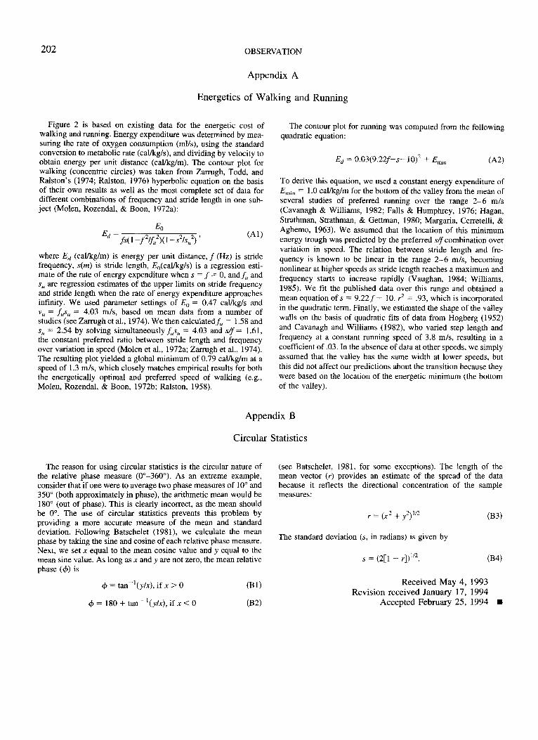
202 OBSERVATION

Appendix A

Energetics of Walking and Running

Figure 2 is based on existing data for the energetic cost of walking and running. Energy expenditure was determined by mea­suring the rate of oxygen consumption (mIls), using the standard conversion to metabolic rate (cal/kg/s), and dividing by velocity to obtain energy per unit distance (cal/kglm). The contour plot for walking (concentric circles) was taken from Zarrugh, Todd, and Ralston's (1974; Ralston, 1976) hyperbolic equation on the basis of their own results as well as the most complete set of data for different combinations of frequency and stride length in one sub­ject (Molen, Rozendal, & Boon, 1972a):

Eo E---..."..--,,-----::-_:_

d - fs(l-f 2/f/)(l- i/s/) , (AI)

where Ed (cal/kglm) is energy per unit distance, f (Hz) is stride frequency, sCm) is stride length, Eo(cal/kg/s) is a regression esti­mate of the rate of energy expenditure when s = f = 0, and fu and Su are regression estimates of the upper limits on stride frequency and stride length when the rate of energy expenditure approaches infinity. We used parameter settings of Eo = 0.47 cal/kg/s and Vu = fusu = 4.03 mis, based on mean data from a number of studies (see Zarrugh et al., 1974). We then calcu1atedfu = 1.58 and Su = 2.54 by solving simultaneously fusu = 4.03 and sIJ= 1.61, the constant preferred ratio between stride length and frequency over variation in speed (Molen et al., 1972a; Zarrugh et al., 1974). The resulting plot yielded a global minimum of 0.79 callkg/m at a speed of 1.3 mis, which closely matches empirical results for both the energetically optimal and preferred speed of walking (e.g., Molen, Rozendal, & Boon, 1972b; Ralston, 1958).

The contour plot for running was computed from the following quadratic equation:

Ed = O.03(9.22f-s-IO)2 + Emin (A2)

To derive this equation, we used a constant energy expenditure of Emin = 1.0 cal/kglm for the bottom of the valley from the mean of several studies of preferred running over the range 2-6 m/s (Cavanagh & Williams, 1982; Falls & Humphrey, 1976; Hagan, Strathman, Strathman, & Gettman, 1980; Margaria, Cerretelli, & Aghemo, 1963). We assumed that the location of this minimum energy trough was predicted by the preferred sIJ combination over variation in speed. The relation between stride length and fre­quency is known to be linear in the range 2-6 mis, becoming nonlinear at higher speeds as stride length reaches a maximum and frequency starts to increase rapidly (Vaughan, 1984; Williams, 1985). We fit the published data over this range and obtained a mean equation of s = 9.22f - 10, ? = .93, which is incorporated in the quadratic term. Finally, we estimated the shape of the valley walls on the basis of quadratic fits of data from Hogberg (1952) and Cavanagh and Williams (1982), who varied step length and frequency at a constant running speed of 3.8 mis, resulting in a coefficient of .03. In the absence of data at other speeds, we simply assumed that the valley has the same width at lower speeds, but this did not affect our predictions about the transition because they were based on the location of the energetic minimum (the bottom of the valley).

Appendix B

Circular Statistics

The reason for using circular statistics is the circular nature of the relative phase measure (0°-360°). As an extreme example, consider that if one were to average two phase measures of 10° and 3500 (both approximately in phase), the arithmetic mean would be 180° (out of phase). This is clearly incorrect, as the mean should be 0°. The use of circular statistics prevents this problem by providing a more accurate measure of the mean and standard deviation. Following Batschelet (1981), we calculate the mean phase by taking the sine and cosine of each relative phase measure. Next, we set x equal to the mean cosine value and y equal to the mean sine value. As long as x and y are not zero, the mean relative phase (<1» is

<I> = tan -I (y/x), if x> 0

<I> = 180 + tan - I(y/x), if x < 0

(BI)

(B2)

(see Batschelet, 1981, for some exceptions). The length of the mean vector (r) provides an estimate of the spread of the data because it reflects the directional concentration of the sample measures:

(B3)

The standard deviation (s, in radians) is given by

s = (2[1 - r])1I2. (B4)

Received May 4, 1993 Revision received January 17, 1994

Accepted February 25, 1994 •