1 2 3

Nonlinear DynamicsAn International Journal of NonlinearDynamics and Chaos in EngineeringSystems ISSN 0924-090X Nonlinear DynDOI 10.1007/s11071-018-4466-9

Geometrically optimal gaits: a data-drivenapproach

Brian Bittner, Ross L. Hatton & ShaiRevzen

1 2 3

Your article is protected by copyright and

all rights are held exclusively by Springer

Nature B.V.. This e-offprint is for personal

use only and shall not be self-archived

in electronic repositories. If you wish to

self-archive your article, please use the

accepted manuscript version for posting on

your own website. You may further deposit

the accepted manuscript version in any

repository, provided it is only made publicly

available 12 months after official publication

or later and provided acknowledgement is

given to the original source of publication

and a link is inserted to the published article

on Springer's website. The link must be

accompanied by the following text: "The final

publication is available at link.springer.com”.

Nonlinear Dyn

https://doi.org/10.1007/s11071-018-4466-9

ORIGINAL PAPER

Geometrically optimal gaits: a data-driven approach

Brian Bittner ·Ross L. Hatton·Shai Revzen

Received: 28 December 2017 / Accepted: 3 July 2018© Springer Nature B.V. 2018

Abstract The study of optimal motion of animals or

robots often involves seeking optimality over a space

of cyclic shape changes, orgaits, specified using alarge number of parameters. We show a data-driven

method for computing the gradient of a cost functional

with respect to a large number of gait parameters byemploying geometric properties of the dynamics to effi-

ciently construct a local model of the system, and then

using this model to rapidly compute the gradients. Our

RLH thanks the National Science Foundation for support underCivil, Mechanical and Manufacturing Innovation grant1653220. SR and BB were funded by Army Research Officegrant W911NF-14-1-0573 and the Rackham Merit Fellowship.

Electronic supplementary material The online version ofthis article (https://doi.org/10.1007/s11071-018-4466-9)contains supplementary material, which is available toauthorized users.

B. Bittner (B)Robotics Department, University of Michigan, Ann Arbor,USAe-mail: babitt@umich.edu

R. L. HattonCollaborative Robotics and Intelligent Systems (CoRIS)Institute and School of Mechanical, Industrial, andManufacturing Engineering, Oregon State University,Corvallis, USAe-mail: ross.hatton@oregonstate.edu

S. RevzenElectrical Engineering and Computer Science Department,Ecology and Evolutionary Biology Department, RoboticsInstitute, University of Michigan, Ann Arbor, USAe-mail: shrevzen@umich.edu

modeling step specifically applies to systems governed

by connection-like models from geometric mechanics,

which encompass a number of high-friction regimes.We demonstrate using our method for optimizing gaits

under noisy, experiment-like conditions by simulat-

ing planar multi-segment serpent-like swimmers in alow Reynolds number (viscous friction) environment.

Our optimization results recover known results for 3-

segment swimmers with a 66 dimensional gait param-eterization, and extend to optimizing the motion of a 9

segment swimmer with a 264 dimensional gait space,

using only 30 simulation trials of 30 gait cycles each.

The data-driven geometric gait optimization approachwe present is designed to operate on noisy, stochas-

tically perturbed dynamics—as noisy and variable as

experimental data—and efficiently optimize a largenumber of parameters. We believe this approach has

the potential to significantly advance our ability to opti-

mize robot gaits with hardware in the loop and to studythe optimality of animal gaits with respect to hypothe-

sized cost functions.

KeywordsGait optimization·Locomotion·Geo-metric mechanics·Oscillator·Data-driven floquet

analysis

1 Introduction

The ability to move effectively through the environ-

ment is both a defining property of animals and a

Author's personal copy

12 3

B. Bittner et al.

highly desirable capability for man-made systems suchas robots and vehicles. Locomotion (aquatic, terres-

trial, and aerial) is most commonly achieved by having

a moving body change shape in a way that producesreaction forces from the environment; these reaction

forces in turn propel the body. A key question in both

robotics and animal research is thus “does a given gaitcycle optimally exploit this propulsive relationship, and

if not, what changes to the gait would improve its per-

formance?”

This paper details a new approach to answeringthese questions, by presenting a practical extension of

geometric gait optimization theory that incorporates

techniques from the data-driven modeling of gaits asoscillators. By efficiently producing a local geometric

mechanics model of the observed motion, we can then

employ this model to rapidly evaluate the gradient of agoal function with respect to gait parameters. Because

this performance simulation is very fast, the number of

gait parameters being optimized can be so large that

estimating such a gradient by direct experimentation isnigh impossible; below we give an example with 264

parameters optimized in 30 trials of 30 cycles each.

The framework presented in this paper is madepossible by combining work in two fields that have

developed largely in parallel. In the field of geometric

mechanics, Hatton has developed a framework for char-acterizing gait efficiency in terms of the length and area

of the cycle in the shape space [8,11,13,23,24]. Apply-

ing these principles to systems that lack an analytical

model remains an open area of investigation, especiallywhen high-dimensionality makes the exhaustive explo-

ration of system dynamics from [5,12] infeasible, or

when considering an animal whose motions we cannotdirectly command.

In the field of oscillator theory, Revzen developed a

set of tools for extracting oscillator-like motion modelsfrom noisy and irregularly spaced data [26,28]. In addi-

tion to the method’s robustness to the intrinsic system

noise of biological and physical systems, it extends well

to high dimensional shape spaces. A limitation, how-ever, is the lack of insight that these models provide for

gait improvements.

Applying the data-driven oscillator and geometricapproaches together enhances their respective capabil-

ities: the data-driven oscillator tools can provide the

geometric models with the specific information neededfor evaluating a performance criterion and its gradient,

improving their predictive power relative to the quan-

tity of available data. Conversely, by viewing the sys-tem as a mechanical connection (as a opposed to a gen-

eral second-order dynamical system) the data-driven

oscillator models can ignore certain aspects of the sys-tem dynamics that are irrelevant to the optimality of the

gait, thus significantly reducing the algorithmic com-

plexity of model extraction.Here, we lay out a framework for combining the geo-

metric insights from Hatton’s work with the data-driven

oscillator model construction from Revzen’s work. Our

combined approach uses noise in the dynamics of a sys-tem that follows a nominal gait cycle to build a model

of the system dynamics in the neighborhood of this gait

cycle. Inserting this model into our geometric tools thenprovides estimates of both how optimal this gait is rel-

ative to nearby cycles and what perturbations can be

applied to the cycle to best improve its performance.This estimation technique has two primary use cases.

– The first is as a tool that allows for verification ofpostulated goal functions for observed animal loco-

motion.

– The second is in field robotics, where an effi-cient, noise resistant gait optimization algorithm

can potentially enable learning effective gaits with-

out requiring precise analytical models of the robotor its interactions with the environment.

2 Contributions

The approach presented in this paper offers a collection

of advantages in speed, scalability, and model reduc-

tion for the estimation of motion models and subse-quent optimization of gaits. These advantages derive

from the use of geometric mechanics models governed

by a connection (the “principal kinematic case” in thelanguage of [21]). The absence of a momentum term

in the equation of motion implies that the contribution

of different segments of motion do not strongly depend

on each other, allowing motion models to be integratedin parallel instead of sequentially in time. With multi-

processor computing becoming cheaper, this offers the

opportunity for dramatic speedups in the computationof motion plans. Additionally, connections expose the

fact that the systems they govern are, for practical pur-

poses, half the dimension of general mechanical sys-tems. As the very name “geometric mechanics” sug-

gests, in these systems, the geometry of motion in body

Author's personal copy

12 3

Geometrically optimal gaits: a data-driven approach

shape space governs the outcome of motions, admit-ting a description with only one dimension per degree

of freedom, instead of the two needed in conventional

Newtonian mechanics. Despite this great promise ofgeometric mechanics models, little work has been done

on producing them in a data-driven way. Developing a

tool for the data-driven creation of such models allowsus to explore their value for both scientific and engi-

neering applications.

Our most significant contribution is the demonstra-

tion of an algorithm for producing data-driven connec-tion models in the neighborhood of a (noisy) rhythmic

motion. Because it estimates linear models as a func-

tion of phase, our algorithm requires a number of cyclesproportional to the state-space dimension, rather than

being exponential in the state-space dimension. No pre-

vious method for data-driven connection estimation hasless than exponential data requirements.

Our second contribution is the demonstration of

a gradient ascent algorithm that can utilize the data-

driven connection models we identify to optimize agoal function. Our algorithm constructs a local model

and estimates the gradient with respect to this fast-to-

integrate connection model. It then steps within thevolume supported by the local model it used. The

power of our algorithm is that it replaces gradient

estimation against the full model or physical systemwith gradient estimation against a fast, easy to par-

allelize model evaluation. This allows policies with

orders of magnitude more parameters to be optimized.

In our example, a 264 parameter policy, optimized with30 trials of 30 movement cycles each, finding strong

solutions from a broad collection of seeded initial

gaits.Below we review the geometric and data-driven

approaches, and then synthesize them into a tool for

simultaneously estimating and optimizing locomotionmodels. Using simulated mechanical swimming plat-

forms, we illustrate the precision of these data-driven

geometric mechanics models and demonstrate that

optimal gaits can be learned with very few trials.Finally, we discuss the utility of the new methods for

both system identification and field robotics.

3 Geometry of locomotion

The first thread of prior work that this paper draws upon

is geometric modeling of locomotion. When analyzing

a mobile deformable system, it is convenient to sep-arate its configuration spaceQ(i.e., the space of its

generalized coordinatesq) into a position spaceGand

a shape spaceR, such that the positiong∈Glocatesthe system in the world, and the shaper∈Rgives the

relative arrangement of the particles that compose it.1

During locomotion, changes in the system’s shapeprovoke reaction forces from the environment that in

turn drive changes in the system’s position. For the pur-

poses of this paper, we adopt a (geometric) locomotion

model

◦g=A(r)r, (1)

whereA,thelocal connection, linearly maps the shape

velocityrto the body velocity◦g= g-1g(i.e., the

position velocity in the body frame’s current forward,

lateral, and rotational directions). The local connec-tion acts similarly to the Jacobian map of a kine-

matic mechanism—it takes the velocity of joints to the

position velocity (here, of the body frame instead ofend effector) that they generate under the constraints

imposed on the system.

We model the cost of changing shape as correspond-ing to the lengthsof the trajectory through the shape

space,

s=

ˆ

drTM(r)dr=

ˆT

0rTM(r)rdt, (2)

whereM is a Riemannian metric on the shape spacethat weights the costs of changing shape in different

directions.

This connection-and-metric model applies to sys-tems that move by pushing directly against their envi-

ronment with negligible accumulated momentum in

“gliding” modes, and whose energetic costs are dom-

inated by internal or external dissipative effects. Thismodel has been analytically derived for swimmers in

viscous fluids [1,13], and experimentally validated for

several robots in dry granular media [5,12,19].The meaning of the cost encoded by the metricM

depends on the system physics, but at a high level it can

be considered as the time it will take the system to exe-cute the motion given a unit power budget. For systems

1 In the parlance of geometric mechanics, this assignsQthestructure of a (trivial, principal)fiber bundle,withGthefiberspaceandRthebase space.

Author's personal copy

12 3

B. Bittner et al.

moving in dry-friction environments,scan be specif-ically taken the energy dissipated while executing the

motion [5]; for the viscous friction model we consider

in this paper,sis the time-integral of the square root ofpower dissipated [13].

3.1 Extremal and optimal gaits

Locomoting systems typically move by repeatedly

executinggaits—cyclic changes in shape that pro-duce characteristic net displacements in position. Such

cycles can be chained together to produce larger

motions through the world.Geometrically, a gaitθis a cyclic trajectory through

the shape space with periodT,

θ:[0,T] →R (3)

θ(0)=θ(T), (4)

and the system shape at any timetwhile executing the

gait isr=θ(t).

Under the locomotion model in (1), the net displace-ment over one cycle of a gait is equal to the path inte-

gral of the local connectionAover that trajectory. By

an extension of Stokes’ theorem, this displacement canbe approximated2as the integral of thecurvatureofA

over a surfaceθabounded by the gait,

gθ=

‰

θgA(r)dr≈

¨

θa

curvatureDA

dA+ Ai,Aj>i. (5)

The curvatureDA(formally, the total Lie bracketor covariant exterior derivative ofA[11]) measures

how much the coupling between shape and position

motions changes across the cycle, and thus how much

displacement the system can extract from a cyclicmotion. Its componentsdAand[Ai,Aj]are the exte-

rior derivative (curl) and local Lie bracket of the system

constraints and, respectively, capture the net forward-minus-backward motion and parallel-parking motion

available to the system. They are calculated as

2The quality of this approximation depends on the choice ofbody frame for the system, which can be optimally selected onceAis calculated in an arbitrary convenient frame. See [8,9,11]forfurther discussion of this point.

dA=j>i

∂Aj

∂ri−∂Ai

∂rjdri∧drj (6)

and

[Ai,Aj]=g-1 ∂(gAj)

∂gAi−

∂(gAi)

∂gAj dri∧drj

(7)

=

⎡

⎣AyiAθj−A

yjAθi

AxjAθi−A

xiAθj

0

⎤

⎦dri∧drj, (8)

where the wedge product dri∧drjis the basis areaspanned by theith andjth basis vectors.

For systems with two shape variables,dAand

[Ai,Aj]have only a single component (on the dr1∧dr2plane), and (5) reduces to a simple area integral whose

integrand is the magnitude ofDA. Extremal gaits for

these systems (maximizing net displacement per cycle)

lie along zero-contours ofDA, maximizing the sign-definite region they enclose.

As a general rule, these extremal gaits are more inter-

esting mathematically than as a motion for a robot oranimal to follow. With the exception of sports such

as basketball that explicitly count steps, displacement-

per-cycle is not a useful quantity to optimize, as it leadsto wasting time or energy eking out all the available dis-

placement in the cycle, instead of executing smaller but

more productive cycles more times. When considering

the optimality of a gait, it is thus typically more usefulto measure its efficiency by dividing the displacement

the gait induces over each cycle by the effort or time

required to execute it.In our model, we take the efficiencyγas the ratio

between net displacementgθit induces and the path-

length costscalculated in (2),γ:=gθs. The path-length cost,s, which in the viscous case determines the

energy dissipated over a cycle under optimal pacing,

can be computed independently of the pacing of the

gait. This enablesγto represent the proper notion ofefficiency for such systems [13]. Note that maximizing

this efficiency is equivalent to maximizing speed at a

given power (or minimizing power for a given desiredspeed), and so gaits with this property are always the

most desirable for effective locomotion, even when the

goal is “move fast” instead of “move efficiently.”As discussed in [13], optimally-efficient gaits are

contracted versions of extremal gaits: they give up low-

Author's personal copy

12 3

Geometrically optimal gaits: a data-driven approach

yb

α1

α2xb

(x, y, θ) 1.5

0

-1.5 1.50

-1.5

α1

α2Curvature

curl + Lie bracket

Constraints

Δxb/gait

0.23

0.23

Maximum-displacement gait

(encloses whole

gait(best ratio of enclosure to perimeter length)

0

0

-0.14

-0.14

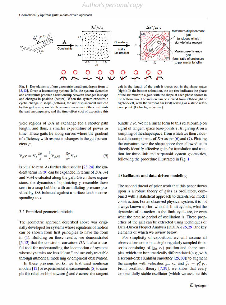
Fig. 1 Key elements of our geometric paradigm, drawn from to[8,13]. Given a locomoting system (left), the system dynamicsand constraints produce a relationship between changes in shapeand changes in position (center). When the system executes acyclic change in shape (bottom), the net displacement inducedby this gait corresponds to how much curvature of the constraintsthe gait encompasses, and the time-effort cost of executing this

gait is the length of the path it traces out in the shape space(right). In the bottom animation, the top row indicates the phaseof the swimmer in a gait, with the shape at each phase shown inthe bottom row. The motion can be viewed from left-to-right orright-to-left, with the vertical bar (red) serving as a static refer-ence point. (Color figure online)

yield regions ofDAin exchange for a shorter pathlength, and thus, a smaller expenditure of power or

time. These gaits lie along curves where the gradient

of efficiency with respect to changes in the gait param-

etersp,

∇pγ=∇pgθ

s=1

s∇pgθ−

gθ

s2∇ps (9)

is equal to zero. As further discussed in [23,24], the gra-

dient terms in (9) can be expanded in terms ofDA,Mand∇M evaluated along the gait. Given these expan-

sions, the dynamics of optimizingγresemble those

seen in a soap bubble, with an inflating pressure pro-

vided byDAbalanced against a surface tension corre-sponding tos.

3.2 Empirical geometric models

The geometric approach described above was origi-

nally developed for systems whose equations of motion

can be shown from first principles to have the formin (1). Building on these results, we demonstrated

[5,12] that the constraint curvatureDAisalsoause-

ful tool for understanding the locomotion of systemswhose dynamics are less “clean,” and are only tractable

through numerical modeling or empirical observation.

In these previous works, we first used nonlinearmodels [12] or experimental measurements [5]tosam-

ple the relationship between◦gandracross the tangent

bundleTR. We fit a linear form to this relationship ona grid of tangent space base-pointsTrR,givingAon a

sampling of the shape space, from which we then calcu-

lated the components ofDAas per (6) and (7). Plotting

the curvature over the shape space then allowed us todirectly identify effective gaits for translation and rota-

tion for three-link and serpenoid system geometries,

following the procedure illustrated in Fig.1.

4 Oscillators and data-driven modeling

The second thread of prior work that this paper draws

upon is a robust theory of gaits as oscillators, com-

bined with a statistical approach to data-driven modelconstruction. For an observed physical system, it is not

always known a priori what this limit cycle is, what the

dynamics of attraction to the limit cycle are, or evenwhat the precise period of oscillation is. These prop-

erties of the gait can be extracted using techniques of

Data-Driven Floquet Analysis (DDFA) [26,29], the key

elements of which we review below.For simplicity of exposition, we will assume all

observations come in a single regularly sampled time-

series consisting of(gn,rn)position and shape sam-ples, which can be numerically differentiated (e.g., with

a second-order Kalman smoother [25,30]) to augment

the samples with velocitiesgn,rn, and◦gn= g

-1ngn.

From oscillator theory [7,29], we know that every

exponentially stable oscillator (which we assume this

Author's personal copy

12 3

B. Bittner et al.

Fig. 2Data-Driven Floquet Analysis applied to a Hopf oscil-lator with system noise. Trajectories of the oscillator convergeto a (noisy) cycle (left plots, three colors, one per trajectory).This cycle appears as a circle in state-space (extreme left) andas sinusoidal time-series (second from left). By differentiation,we obtain vector field samples at the data points (middle). Weestimate the limit cycle as a function of phase (second from

right) computed using the phase estimator from [28] providing acanonical map from every trajectory point to a point with iden-tical phase on the limit cycle (thin black lines, right plots). Suchsurfaces of constant phase—isochrons—form radial lines in the(particularly simple) case of the Hopf oscillator. (Color figureonline)

to be) can be parameterized with a phase coordinate

ϕ:R→[0,T)⊂Rbased on the following rules:

1. Each point on the limit cycle has a unique phasevalue, spaced such that limit cycle trajectories

advance in phase at rateϕ=1.

2. Each point not on the limit cycle inherits its phase

value from a corresponding point on the limit cycle,selected such that trajectories starting at the two

points ultimately converge. The set of all points

sharing a value ofϕare called anisochronofthe oscillator, and the trajectories of the oscillator

advance across isochrons such thatϕ=1every-

where.

Our modeling process was as follows: we assigned eachsamplena phaseϕnvia aphase estimatorsuch as that

presented in [27], which takes the multivariate time-

series of measured data from an oscillator and gives aphase estimate for every data point. Figure2provides

a visual example.

Once we grouped the samples by phase, we modeledthe limit cycle (nominal-gait-as-executed) by comput-

ing a pair of Fourier seriesθ0andωwith respect to the

phase:θ0(ϕn)≈rnwas fitted to the sampled shapes,

andω(ϕn)≈ rnwas fitted to the shape velocities.Because each ofθ0andωis computed from its own

noisy dataset, the conditionθ0=ωneed not be satisfied

after this fitting procedure. We create a self-consistentmodelθof the limit cycle by producing the analytical

integral ofω, and using a matched filter to combine

this integral with theθ0estimate to obtain a single self-consistent cyclic trajectory. Past experience [26] has

shown that this estimation procedure provides a better

representation of the limit cycle than the directly fitted

shape modelθ0.

5 Data-driven modeling of the connection

The gait analysis methods described in Sect.3pro-

vide a powerful link between gaits’ optimality and theirgeometry. Their utility, however, depends on having

a model for how small shape changes induce body

motion changes. For systems that experience com-plex interactions with their environments, such models

are not readily available from first principles [even if

their net effect can be modeled as the linear relation-

ship in (1)], and exhaustive empirical evaluations [5]become infeasible as we move to system with many

shape variables and/or limited control affordances.

Conversely, the data-driven methods describedin Sect.4are able to extract a meaningful model of

a system from noisy measurements. This model, how-

ever, is limited to the specific gait being executed anddoes not provide context for comparing the gait against

other motions the system could execute, or for optimiz-

ing the motion.

Our key innovation in this paper is based on theobservation that the data-driven modeling approach can

allow us to quickly build up a first-order model of the

connection in a tube around a given gait cycle. In turn,the first-order model allows us to rapidly compute the

influence of any gait change within the model’s domain

of validity. Such computations allow us to numericallyapproximate, at this given gait cycle, the gradient of any

goal function computed from a gait with respect to any

Author's personal copy

12 3

Geometrically optimal gaits: a data-driven approach

parameterization of gaits—even when this parameter-ization is fairly high dimensional and requires a great

many “simulations” of gaits.

In this innovation, we exploit two propertiesof the geometric model: (1) the variational opti-

mizer/definition of optimality described in (9) only

needs to knowDAalong the given gait to identify thedirection in which that gait can be perturbed to best

improve performance. (2)DA, being a two-form and

thus a linear map, can be reconstructed at every point

along a gait cycle using regressions applied to the rela-tionship betweengandrcollected from experiments.

5.1 Analytic approximation of the connection near a

gait

In this section, we introduce an approximation of the

mechanical connection and the cost metric, both cen-

tered about a nominal gait. We then construct a proce-dure to estimate the local model elements from data. As

discussed in Sect.4, a gait cycleθ(·)can be extracted

from shape datarvia Data-Driven Floquet Analysis.Perturbations from this phase-averaged behavior are

written asδ(t):=r(t)−θ(t). These terms can be

used to construct a first-order approximation ofA(·)ina neighborhood of the point-set Imθusing its Taylor

series,

Aki(r)ri=Aki(θ+δ)r

i≈ Aki(θ )+∂Aki∂rj(θ )δj ri,

(10)

where, as per Einstein index notation,Akicorresponds

to the element in thek-th row andi-th column ofA.Including the derivative of the connection across the

shape space allows us to estimate the connection for

behaviors that are not on the current gait cycleθ(·),and that thus provide velocity samples in nearby, but

not identical, tangent spaces of the shape space.

It is important to stress that∂Ak

∂r is not simply theHessian matrix ofgkwith respect toraround points

on the gait, i.e., it is not the gradient of a gradient. The

Hessian could only be computed ifgwereafunctionofr, but it is not. In fact, locomotion via gaits would

be impossible if it were such a function since a cycli-

cal change inrcould not induce a net change ing.In particular, Hessians are symmetric operators, and

the difference term that appears when calculatingdAk

in (6) directly measures the system’s ability to locomotealong thek-th direction in terms of the asymmetry of∂Ak

∂r. Similarly, the[Ai,Aj]term from (7) measures

the covariant asymmetry of∂gA∂g when the connectionis expanded from local to global coordinates.

5.2 EstimatingA(θ )andDA(θ )from data

Our input data was time series of the system shapern,

shape velocityrn, and observed body velocity◦gn,at

sufficiently many time pointsn=1...N.Webegin

our system identification process by applying the gait

extraction algorithm described in Sect.4, producingFourier series models ofθ(·)and ofθ(·). We then select

Mevenly spaced values of phase,ϕ1...ϕM, to obtain

θm:=θ(ϕm)andθm:=θ(ϕm)—the shapes and shape

velocities of a system that is following the gait cycleprecisely. We use these as the points at which we esti-

mate the connection and its derivative.

For each cycle pointθm, we collect all shapesrnthatare sufficiently close, i.e.,nsuch thatrn−θm <δmax.

For notational simplicity, when both indexnand index

mappear in an equation below, we take the values ofnto be restricted to only those sufficiently close time-

series points. We now define the offset between the

shape sample and its current on-gait reference point as

δn:=rn−θm.Within eachθmneighborhood, we now estimate the

local connection and its derivatives by using a linear

regression to find the slopes of the relationship between◦g,r, andδ. Naively, this regression is the solution to

the Generalized Linear Model formed by placing the

Taylor-series expansion ofAfrom (10) into the loco-motion model from (1):

◦gkn∼ Aki r

in+

∂Aki∂rj

δjnrin, (11)

whereAkiare theMseparate estimates ofAki(θm)and

∂Aki∂rj

are theMseparate estimates of∂Aki∂rj(θm).

When applied to samples generated from an oscilla-tor as illustrated in Fig.2, this straightforward regres-

sion is biased by the shape velocity samples being

centered aroundr= θmrather thanr=0. We cor-rect for this bias by re-centering the regression around

A(θm)θm. We separate the perturbations of the shape

Author's personal copy

12 3

B. Bittner et al.

Observed shape motionand averaged gait

Velocity samples in neighborhoodof one point on gait

Geometric locomotion model from regressionbetween shape and position velocities

x

α1

α2

α2 α2α1 α1

x

Fig. 3Illustration of the connection estimation process. We takethe rhythmic data, group it by phase, and average using a Fourierseries to obtain a periodic gait (left; red cycle). We collect shapevelocity and body velocity data (middle; rooted arrows) withinthe neighborhood of point on the gait (black oval, left; zoomedin area, middle). Using these data, we fit a first-order approxi-

mation of the connection model (black planes; right). We repeatthis process for a collection of points on the gait cycle at fixedphase intervals, and fit the parameters of the estimated modelswith a Fourier Series to obtain a model of the connection thatsmoothly varies with phase. Further detail in Sect.5.2. (Colorfigure online)

velocity away from the gait cycle velocity from the

influence of the gait cycle velocity itself by defining

δn:= rn−θm, and re-writing the GLM of (11) as (forvelocity componentkand each value ofm):

◦gkn∼C

k+Bkjδjn+ Aki δ

in+

∂Aki∂rj

δjnδin (12)

whereCk:=Akiθiis the connection applied to the

(unmodified) gait cycle shape velocity, andBkj:=∂Aki∂rjθiis the interaction effect of shape offset and shape

velocity applied to the (unmodified) gait cycle shape

velocity. Here,Ckis a constant (withk,mfixed); andBkis a (“co-”)vector that acts on shape offsets from the

gait, rather than on conventional tangent vectors. The

Aki element is a true co-vector that acts on velocity

offsets away from the typical gait velocity, and∂Aki∂rj

is the interaction matrix of shape offsets and shape

velocity offsets, offset being taken relative to the nom-inal gait cycleθ(Fig.3).

We compute the regression by writing it in matrix

form and thereby posing the least-squares problem (foreachkandm; indiceskandmelided below for clarity):

⎡

⎢⎣

◦g1...◦gN

⎤

⎥⎦=

⎡

⎢⎣

1,δ1,δ1,δ1⊗δ1.........

...

1,δN,δN,δN⊗δN

⎤

⎥⎦·C,Bj,Ai,

∂Ai∂rj

T

(13)

where indicates “estimated” and⊗is the outer prod-

uct. For addimensional shape space, the row of

unknowns on the right consists of 1+d+d+d2

elements.

Once we have the model for everym, we construct

a Fourier series model of each of the matrices of theGLM, allowing them to be smoothly interpolated at

any phase value.

5.3 Estimating the metric

In the same manner as we estimateA, we can estimate

a Riemannian effort-metricM on the shape space byrecording the differential cost of motionsalong with

the system kinematics, and then fitting these costs to a

linearized expansion of (2) taken at the pointsθmusingthe matchingnindices,

s2n∼rnT M +

∂M

∂rjδjn rn. (14)

This regression suffers from the afore-mentioned bias

stemming from thervalues being centered around

θinstead of 0;, so we recenter it in a similar man-ner as in (13). Additionally, becauseM is a symmet-

ric tensor, onlyd2 elements need to be estimated,

reducing by about half the number of quantities toestimate. Details of this regression calculation are in

“Appendix A”.

Author's personal copy

12 3

Geometrically optimal gaits: a data-driven approach

5.4 Comparison of estimates to previous work

This process is analogous to the processes we described

for empirically estimatingAand its derivatives in [5,12], but offers some distinct advantages.

In our previous work, the shape velocity samples to

identifyAat a point all had to be in the tangent spaceof that point. Here, we have relaxed that requirement

by fitting to a linearized expansion of (1) instead of (1)

itself.

Furthermore, since our regression here uses intrin-sic noise in the system, it provides an estimate of the

average behavior under noise. The average behavior

of a system when noise is added depends also on thevariance of the noise. In the analysis here, we account

for the actual noise present in the system, rather than

treating it as mere measurement error of a deterministicsystem.

The presence of system noise and the form of the

linearized expansion allow for collection of data over a

singular repeated gait cycle, rather than collection overthe whole shape space (as was done for the prior model

estimation methods).

5.5 Assumptions for the modeling estimation

We make the following assumptions for modeling: (1)

the deterministic part of the systems time evolution is

governed by a connection; (2) the dynamics are sub-ject to sufficient IID (independent and identically dis-

tributed) system noise to allow them to be identified;

(3) noise is sufficiently small to allow a distinct rhyth-mic motion to be observed and modeled as a limit cycle

oscillator representing a gait. For gait optimization, we

further assume that the system is fully actuated and ableto follow (on average) any trajectories we command.

6 Performance of the data-driven models

To benchmark the accuracy of our data-driven geomet-

ric modeling process, we compared its prediction of

the body velocity for a test system against three systemmodels that had various levels of knowledge about the

“true” system dynamics used in the simulation. The test

system had a geometric locomotion model of the formin (1), and its shape trajectories were generated via a

noisy oscillator like that illustrated in Fig.2.

6.1 Reference models

As described in Sect.5, we used a data-driven process

to construct a phase varying first-order model ofAatpointsθmalong our observed gait cycle. Eachrndata

point from the (noisy) trial was associated with a corre-

sponding (phase-matched) pointθnon the gait cycle,3

which allowed us to compare several different models

for the body velocity:

1. Theground truth model

◦gG,n=A(rn)rn, (15)

in which each(rn,rn)pair is passed directly to thesimulator dynamics, giving

2. The fullydata-driven model, where the regression

estimates of the Taylor expansion ofAare usedto approximateAat points off of the gait cycle,

and◦gD,nis given by (12), used with the quantities

estimated from (13).

3. Ananalytic model

◦gA,n=A(θn)rn+

∂A

∂r(θn)δnrn (16)

that uses a Taylor-series expansion of the simula-tor model computed at the same point as the data-

driven model, without using any regression or sim-

ulation data. This model tests the correctness of the

regression in the data-driven model.4. Atemplate projection model

◦gT,n=A(θn)θn. (17)

that projects each(rn,rn)data point onto its corre-

sponding(θn,θn)values for the gait cycle that was

used to derive the data-driven model. This approx-

imation tests how much additional information isgained from the higher order term in the Taylor

expansion.

Note that the template approximation in (17) can be

considered as the leading term of the analytical approx-

imation (after separatingrnintoθnandδncomponents),

3These phase-matchedθnpoints can be individually computedfor eachrn, and so are not restricted to the previously-sampledθmvalues. Similarly, the estimates ofAand its derivative fromSect.5.1are computed as Fourier series, and can thus be inter-polated to anyθn.

Author's personal copy

12 3

B. Bittner et al.

A

B

C

Fig. 4Comparison of model accuracy for 3 link and 9 link swim-mers.aWe drove each platform to follow the extremal gait forthe three-link swimmer (black) generating 30 strokes (blue andred; plotted on first two principal components). Of these, weplotted Cycles 13–18 (red) in the time domain (b), showing theadditional motion predicted beyond the template model by theground truth model (black), the data-driven model (teal), andthe analytic model (red). Because both analytic and data-driven

models follow the ground truth closely, we also plotted a scatterplot of their errors as a function of phase (c), showing that thedata-driven model (teal) has zero average error, unlike the ana-lytic (red) model. As the number of DOF grows (right; 9 linkplots) the mean (solid) and variance (dashed) of the data-drivenmodel (teal) become smaller than those of the analytic model(red). (Color figure online)

and that the partial-derivative terms in (12) and (16)contain the information required to predict the effect

of modifying the gait limit cycle.

6.2 Simulation setup: swimming with system noise

For our baseline system model, we used a three-

link Purcell swimmer [22] modeled as described in

[10]. This system moves through a viscous fluidwith linear drag, which we take as having a 2:1lat-

eral/longitudinal ratio. To demonstrate the ease with

which we can extend our approach to systems withhigher-dimensional shape spaces, we also considered a

nine-link swimmer. Both are pictured in Fig.4part A.

To simulate the effects of noise in the shape dynam-

ics (e.g., weak or imprecise shape control), we gen-erated the shape trajectories from sample paths of a

(Stratonovich) stochastic differential equation, injected

into the shape space:

dϕ=1dt+η◦dWθ

dδ=−(α δ)dt+η◦dWδ,

r(t):=θREF(ϕ(t))+δ(t). (18)

whereθREF(·)was a reference motion we specified as a

Fourier series;αwas the coefficient of attraction bring-ing the system back to the reference gait cycle; andη

was a noise magnifier for the Weiner processesdW

driving both phase noise and shape noise.For all simulations in this paperα=0.05 andη=

0.025, chosen based on the superficial similarity the

noisy trajectory ensembles have to experimental datawe have worked with.

6.3 Model accuracy results

To illustrate the performance of our data-driven mod-els, we examined the differences between motion pre-

dicted by the models in Sect.6.1when the reference

gait was the extremal gait maximizing motion in thexdirection, known from [9,33]. We specifically chose

an extremal gait as our example because non-extremal

Author's personal copy

12 3

Geometrically optimal gaits: a data-driven approach

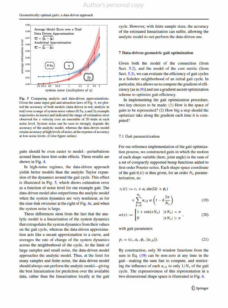
Fig. 5Comparing analytic and data-driven approximations.Given the same input gait and attraction laws of Fig.4, we plot-ted the accuracy of both models (data-driven in red; analytic inteal) over a range of system noise values (0.5η,ηand 2ηexampletrajectories in insets) and indicated the range of estimation errorobserved forxvelocity over an ensemble of 20 trials at eachnoise level. System noise can be seen to strongly degrade theaccuracy of the analytic model, whereas the data-driven modelretains accuracy at high levels of noise, at the expense of accuracyat low-noise levels. (Color figure online)

gaits should be even easier to model—perturbations

around them have first-order effects. These results are

shown in Fig.4.In high-noise regimes, the data-driven approach

yields better models than the analytic Taylor expan-

sion of the dynamics around the gait cycle. This effect

is illustrated in Fig.5, which shows estimation erroras a function of noise level for our example gait. The

data-driven model also outperforms the analytic model

when the system dynamics are very nonlinear, as forthe nine-link swimmer at the right of Fig.4c, and when

the system noise is large.

These differences stem from the fact that the ana-lytic model is a linearization of the system dynamics

that extrapolates the system dynamics from their values

on the gait cycle, whereas the data-driven approxima-

tion acts like a secant approximation to a curve, andaverages the rate of change of the system dynamics

across the neighborhood of the cycle. At the limit of

large samples and small noise, the data-driven modelapproaches the analytic model. Thus, at the limit for

many samples and finite noise, the data-driven model

should always out-perform the analytic model—givingthe best linearization for prediction over the available

data, rather than the linearization locally at the gait

cycle. However, with finite sample sizes, the accuracyof the estimated linearization can suffer, allowing the

analytic model to out-perform the data-driven one.

7 Data-driven geometric gait optimization

Given both the model of the connection (from

Sect.5.2), and the model of the cost metric (fromSect.5.3), we can evaluate the efficiency of gait cycles

in a Sobolev neighborhood of an initial gait cycle. In

particular, this allows us to compute the gradient of effi-ciency [as in (9)] and use a gradient ascent optimization

scheme to optimize gait efficiency.

In implementing the gait optimization procedure,two key choices to be made: (1) How is the space of

gaits to be represented? (2) How big a step should the

optimizer take along the gradient each time it is com-

puted?

7.1 Gait parametrization

For our reference implementation of the gait optimiza-

tion process, we constructed gaits in which the motion

of each shape variable (here, joint angle) is the sum ofa set of compactly supported bump functions added to

first-order Fourier series. Each shape-space coordinate

of the gaitθi(t)is thus given, for an orderNoparame-terization, as:

ri(t):=ci+aisin(t+φi)

+

No

k=0

ui,kw t−k2π

No(19)

w(x):=1+cos(xNo)|xNo|<π

0 |xNo|≥π, (20)

with gait parameters

pi=(ci,ai,φi,{ui,k}). (21)

By construction, only 30 window functions from thesum in Eq. (19) can be non-zero at any time in the

gait—making the sum fast to compute, and restrict-

ing the influence of eachui,kto only 1/Noof the gaitcycle. The expressiveness of this representation in a

two-dimensional shape space is illustrated in Fig.6.

Author's personal copy

12 3

B. Bittner et al.

elliptical approximation

phase-partitioned splines

full shape trajectory

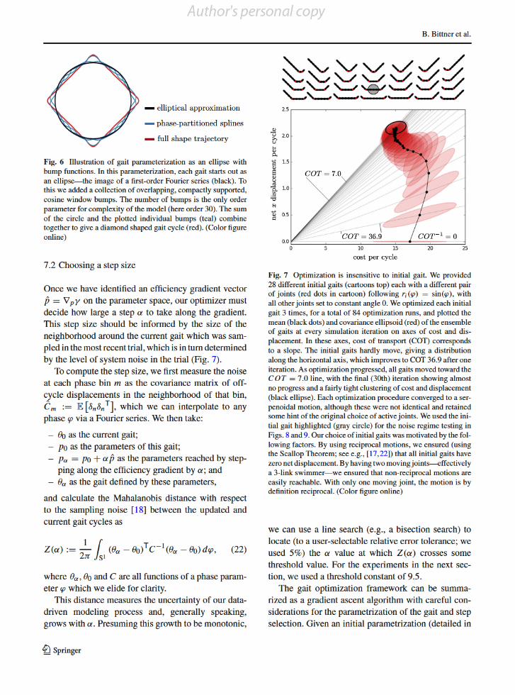
Fig. 6Illustration of gait parameterization as an ellipse withbump functions. In this parameterization, each gait starts out asan ellipse—the image of a first-order Fourier series (black). Tothis we added a collection of overlapping, compactly supported,cosine window bumps. The number of bumps is the only orderparameter for complexity of the model (here order 30). The sumof the circle and the plotted individual bumps (teal) combinetogether to give a diamond shaped gait cycle (red). (Color figureonline)

7.2 Choosing a step size

Once we have identified an efficiency gradient vector

p=∇pγon the parameter space, our optimizer must

decide how large a stepαto take along the gradient.This step size should be informed by the size of the

neighborhood around the current gait which was sam-

pled in the most recent trial, which is in turn determined

by the level of system noise in the trial (Fig.7).To compute the step size, we first measure the noise

at each phase binmas the covariance matrix of off-

cycle displacements in the neighborhood of that bin,

Cm :=EδnδnT, which we can interpolate to any

phaseϕvia a Fourier series. We then take:

–θ0as the current gait;–p0as the parameters of this gait;

–pα=p0+αpas the parameters reached by step-

ping along the efficiency gradient byα; and

–θαas the gait defined by these parameters,

and calculate the Mahalanobis distance with respect

to the sampling noise [18] between the updated and

current gait cycles as

Z(α):=1

2π

ˆ

S1(θα−θ0)

TC−1(θα−θ0)dϕ, (22)

whereθα,θ0andCare all functions of a phase param-

eterϕwhich we elide for clarity.

This distance measures the uncertainty of our data-driven modeling process and, generally speaking,

grows withα. Presuming this growth to be monotonic,

Fig. 7Optimization is insensitive to initial gait. We provided28 different initial gaits (cartoons top) each with a different pairof joints (red dots in cartoon) followingri(ϕ)=sin(ϕ), withall other joints set to constant angle 0. We optimized each initialgait 3 times, for a total of 84 optimization runs, and plotted themean (black dots) and covariance ellipsoid (red) of the ensembleof gaits at every simulation iteration on axes of cost and dis-placement. In these axes, cost of transport (COT) correspondsto a slope. The initial gaits hardly move, giving a distributionalong the horizontal axis, which improves to COT 36.9 after oneiteration. As optimization progressed, all gaits moved toward theCOT=7.0 line, with the final (30th) iteration showing almostno progress and a fairly tight clustering of cost and displacement(black ellipse). Each optimization procedure converged to a ser-penoidal motion, although these were not identical and retainedsome hint of the original choice of active joints. We used the ini-tial gait highlighted (gray circle) for the noise regime testing inFigs.8and9. Our choice of initial gaits was motivated by the fol-lowing factors. By using reciprocal motions, we ensured (usingthe Scallop Theorem; see e.g., [17,22]) that all initial gaits havezero net displacement. By having two moving joints—effectivelya 3-link swimmer—we ensured that non-reciprocal motions areeasily reachable. With only one moving joint, the motion is bydefinition reciprocal. (Color figure online)

we can use a line search (e.g., a bisection search) tolocate (to a user-selectable relative error tolerance; we

used 5%) theαvalue at whichZ(α)crosses some

threshold value. For the experiments in the next sec-tion, we used a threshold constant of 9.5.

The gait optimization framework can be summa-

rized as a gradient ascent algorithm with careful con-siderations for the parametrization of the gait and step

selection. Given an initial parametrization (detailed in

Author's personal copy

12 3

Geometrically optimal gaits: a data-driven approach

Sect.7.1), we collect experimental data (30 cycles inour results section) and compute the local motion-and-

metric models. We extract a gradient on the efficiency

of a motion with respect to the gait parameters by sam-pling many gaits in the neighborhood of the current

policy, using the estimated local model to predict the

performance of each sampled gait. We then determinethe magnitude of the step size as described in Sect.7.2.

This allows the next gait parametrization to represent

a behavior that is reliably informed by the data of the

prior trial. Once the next gait is selected, we collectexperimental data, repeating the above process. The ter-

mination criterion for the gradient ascent algorithm is

a pre-specified number of iterations. A more advancedtermination criterion will be explored in future work.

8 Swimming gait optimization results

As a demonstration of our gait optimization framework,

we applied our algorithm to a 9-link chain “swimmer”.All swimming behaviors shown were optimized with

respect to the efficiency metricγ= gθs, which we

report in units of body lengths per unit time at unit

power. For any given power budget, this efficiencyis inversely proportional to the mechanical cost of

transport.

8.1 Optimization is robust to choice of initial condition

One important test of an optimization algorithm is

its ability to achieve good outcomes irrespective of

initial conditions. To test this ability, we providedthe system with gaits in which two selected joints

follow identical sinusoidal inputs (no phase offset and

amplitude of 1), the other joints attempt to hold at zeroangle, and all joints are subjected to noise as discussed

in (18). The power costs of these gaits depended on

the lengths of the segments between the active joints,

and, as illustrated in Fig.9, as reciprocal motions, theyproduced no net displacement.

From each of these initial conditions, our optimizer

consistently converged (within 30 trials at 30 cycles pertrial) to gaits with a cost of transport of 7.0±0.7. As

illustrated in Fig.8, these resulting motions were very

close to ellipses embedded in the eight-dimensionalshape space, and produced serpenoid undulations trav-

eling along the length of the swimmer. Qualitatively,

Fig. 8Visualization of gaits throughout an optimization. Weprojected all gaits onto the first two principal components of thefinal gait (viewed as embedded inR8) and plotted the projec-tion of thexmotion connection on that subspace (arrows). Theinitial gait (top cartoon), allowing only two joints to move (reddots in cartoon swimmer), is a line in the shape space coordi-nates (black line). The following iterations expand this contouras an ellipse and eventually embellish the ellipse with bumps(red closed ovals) leading to the final gait (black oval) and theserpenoid shape (bottom cartoon). (Color figure online)

the motions are in agreement with the conclusionsabout optimal swimming behavior in [31], with the

exception of maximizing the amplitude of the undu-

lations at the mid-body of the swimmer. In this case,the amplitudes of the discovered gait are typically

maximized near the joints that are excited in the initial

gait. The reason for the discovery of this family of

gaits and their relation to the global optimum in [31]will be the subject of future work.

8.2 Robustness to noise level

A second test of optimizer performance, which is

of particular importance to hardware-in-the-loopoptimization, is its ability to tolerate a variety of

noise levels and produce comparably good results. To

demonstrate this ability, we took a single starting gait(in which the active joints are each set two links in

from the end, as illustrated in Fig.8) and optimized its

motion under different levels of system noise.

For all four noise regimes tested, the system con-verged to serpenoidal motions with geometrically sim-

ilar shapes (similar ratio of wavelength to amplitude),

but with different numbers of waves along the body. Asillustrated in Fig.8, the gaits found at different noise

levels have similar costs of transport (with mean values

ranging from 6.9to7.7), but the systems at higher noiselevels tended toward gaits that were high-cost/high-

displacement, at the expense of some efficiency.

Author's personal copy

12 3

B. Bittner et al.

Fig. 9Course of optimization under different levels of noise.We started with the same initial gait (gray circle highlight inFig.7and top cartoon in Fig.8), but multiplied the noise levelηof Eq. (18)by0.5,1.,1.5,2 (colors yellow, red, teal, andgreen, respectively). For each noise level, we plotted an examplesimulation to illustrate the noise level (ovals framed in color;top). We ran 48 optimizations at each noise level, allowing 60iterations of 30 swimming cycles each, and plotted the mean(circle marker) and covariance (translucent ellipses) of thesetrials at every iteration of the algorithm, highlighting the finalmean (black dot) and covariance (black ellipse). All gaits startedunable to move, and reached COT 7.3±0.4 with high-noiseoptimal gaits being slightly less efficient than low-noise gaits(COT of mean 7.7 vs. 6.9). The two lower noise level achievedindistinguishable cost. It is notable that at higher noises, opti-mization moved away from the origin, producing larger motionswith larger cost. (Color figure online)

Additionally, we note that at all noise levels, thesystems initially modified their gait to increase their

net displacement, then “pulled left” on the graph to

reduce the cost of producing this displacement. The

step sizes between trials are smaller on the low-noisesystems, as they experience smaller perturbations

during the trials, and thus have a lower bound on step

size as discussed in Sect.7.2.

9 Conclusions, limitations, and future work

We have presented two main contributions: (1) amethod for locally modeling a connection and a cost

metric in the neighborhood of a gait cycle, based

solely on the observation of noisy trajectories; (2)an algorithm for gait optimization that employs this

method for gradient climbing.

Our modeling relied strongly on system noise toproduce sufficient excitations to allow us to employ

regression and identify the structure of the dynamics

at every phase of the cycle. In this, there is both astrength and a weakness. The strength comes from

exploiting noise and being able to model systems with

levels of noise comparable to those we have observedin animal and robot data. The weakness comes from

relying on noise to be “system” noise—i.e., arising

from true changes in the system state rather than from

measurement errors. Measurement noise could masksome of the structure we expose by regression. It could

also suggest to the optimization to move in a direction

that is not achievable by the actual hardware.The great strength of our gait optimization algo-

rithm is that it decouples the dimension of the gait

parameter space from the dimension of the shape spaceand the number of trials needed. For a shape space

of dimensiond, orderdcycles are needed to identify

the model. Once the model is identified for a gait,

numerical evaluations of gait perturbations are veryquick, and allow the goal function to be differentiated

with respect to hundreds of variables with little effort.

Some natural extensions of our work includeexpanding to a broader class of data-driven models

outside those systems which admit connection-like

models [2,4,20]. This could enable comparisonbetween analysis of discovered gaits from the data-

driven optimizer with geometric analysis on articulated

swimming in more complex fluids [14–16]. One nat-

ural question which arises is that of systems that are“nearly” geometric—is there a useful and easy to

identify notion of “nearly” geometric that translates to

good predictive ability of geometric tools?Improvements to regression, phase estimation, and

state estimation could enhance our results even more;

in particular, other approaches to gradient ascentstep-size choice seem to hold some promise. Elab-

orating further the relationship between noise level

and which gaits are optimal may provide new insights

into biological mechanisms of robust locomotion.Expanding to broader notions of asymptotic phase

of normally hyperbolic attractors other than limit

cycles [6], our methods could perhaps be extended tooptimize control policies on more elaborate attractors.

Direct extensions of this work are to test our algo-

rithm on physical hardware-in-the-loop optimizationproblems in robotics. We have also applied our algo-

rithm toC. elegansswimming data kindly provided by

Author's personal copy

12 3

Geometrically optimal gaits: a data-driven approach

[32], allowing us to asses optimality of low Reynoldsnumber swimming gaits of these animals [3].

Compliance with ethical standards

Conflicts of interestConflict of Interest: The authors declarethat they have no conflict of interest.

Appendix A: Regression for estimating the cost

metric

The regression for computation of the metricM is

centered aboutθandθ, similarly to the constructionof the regression for the connectionA. The metric

approximation now takes the form:

s2n∼(θn+δnT)M +

∂M

∂rjδjn (θn+δn) (23)

leading to the regression:

⎡

⎢⎢⎢⎣

s21

.

.

.

s2N

⎤

⎥⎥⎥⎦=

⎡

⎢⎢⎢⎣

1,δ1,δ1⊗δ1,δ1,δ1⊗δ1, δ1⊗δ1⊗δ1......

.

.

....

.

.

.

1,δN,δN⊗δN,δN,δN⊗δN,δN⊗δN⊗δN

⎤

⎥⎥⎥⎦·RT,

(24)

R= M i,jθiθj,M i,jθi,M i,j,∂M i,j

∂rkθiθj,

∂M i,j

∂rkθj,

∂M i,j

∂rk

(25)

Here the modified exterior product⊗includes only theupper triangular elements, i.e.,x⊗y=[...,xiyj,...]

s.t.i≤ j. Following (14), at eachmwe solved for

1+d+ d2 +d+d

2+dd2 ≈12d3unknowns to

construct our model of the metric.

References

1. Avron, J.E., Raz, O.: A geometric theory of swimming:Purcell’s swimmer and its symmetrized cousin. New J.Phys.9(437), (2008).https://doi.org/10.1088/1367-2630/10/6/063016

2. Bazzi, S., Shammas, E., Asmar, D., Mason, M.T.: Motionanalysis of two-link nonholonomic swimmers. NonlinearDyn.89(4), 2739–2751 (2017).https://doi.org/10.1007/s11071-017-3622-y

3. Bittner, B., Revzen, S.: What do nematode swimming gaitsoptimize? In: The Society for Integrative and ComparativeBiology Annual Meeting (poster) (2018)

4. Bloch, A.M., Krishnaprasad, P., Marsden, J.E., Murray,R.M.: Nonholonomic mechanical systems with symmetry.

Arch. Ration. Mech. Anal.136(1), 21–99 (1996).https://doi.org/10.1007/bf02199365

5. Dai, J., Faraji, H., Gong, C., Hatton, RL., Goldman, DI.,Choset, H.: Geometric swimming on a granular surface.In: Proceedings of the Robotics: Science and SystemsConference, Ann Arbor, Michigan, https://doi.org/10.15607/rss.2016.xii.012(2016)

6. Eldering, J., Kvalheim, M., Revzen, S.: Global linearizationand fiber bundle structure of invariant manifolds. arXivpreprintarXiv:1711.03646(2017)

7. Guckenheimer, J., Holmes, P.: Nonlinear Oscillations,Dynamical Systems, and Bifurcations of Vector Fields.Springer, New York (1983). https://doi.org/10.1007/978-1-4612-1140-2

8. Hatton, R.L., Choset, H.: Geometric motion planning: thelocal connection, Stokes’ theorem, and the importance ofcoordinate choice. Int. J. Rob. Res.30(8), 988–1014 (2011).https://doi.org/10.1177/0278364910394392

9. Hatton, R.L., Choset, H.: Geometric swimming at low andhigh reynolds numbers. IEEE Trans. Rob.29(3), 615–624(2013a).https://doi.org/10.1109/tro.2013.2251211

10. Hatton, R.L., Choset, H.: Geometric swimming at low andhigh reynolds numbers. IEEE Trans. Rob.29(3), 615–624(2013b).https://doi.org/10.1109/tro.2013.2251211

11. Hatton, R.L., Choset, H.: Nonconservativity and noncom-mutativity in locomotion. Eur. Phys. J. Spec. Top. Dyn.Anim. Syst.224(17–18), 3141–3174 (2015).https://doi.org/10.1140/epjst/e2015-50085-y

12. Hatton, R.L., Choset, H., Ding, Y., Goldman, D.I.: Geomet-ric visualization of self-propulsion in a complex medium.Phys. Rev. Lett.110(078), 101 (2013).https://doi.org/10.1103/physrevlett.110.078101

13. Hatton, R.L., Dear, T., Choset, H.: Kinematic cartographyand the efficiency of viscous swimming. IEEE Trans. Rob.(2017).https://doi.org/10.1109/tro.2017.2653810

14. Kanso, E., Newton, P.: Locomotory advantages to flappingout of phase. Exp. Mech.50(9), 1367–1372 (2010).https://doi.org/10.1007/s11340-009-9287-9

15. Kanso, E., Marsden, J.E., Rowley, C.W., Melli-Huber,J.B.: Locomotion of articulated bodies in a perfect fluid. J.Nonlinear Sci.15(4), 255–289 (2005).https://doi.org/10.1007/s00332-004-0650-9

16. Kelly, SD., Pujari, P., Xiong, H.: Geometric mechanics,dynamics, and control of fishlike swimming in a planarideal fluid. In: Natural Locomotion in Fluids and onSurfaces, Springer, pp. 101–116,https://doi.org/10.1007/978-1-4614-3997-4_7(2012)

17. Lauga, E.: Life around the scallop theorem. Soft Matter7(7),3060–3065 (2011).https://doi.org/10.1039/c0sm00953a

18. Mahalanobis, P.: On the generalized distance in statistics.Proc. Natl. Inst. Sci. India2(1), 49–55 (1936)

19. McInroe, B., Astley, HC., Gong, C., Kawano, SM.,Schiebel, PE., Rieser, JM., Choset, H., Blob, RW., Gold-man, DI.: Tail use improves performance on soft substratesin models of early vertebrate land locomotors. Science353(6295):154–158, https://doi.org/10.1126/science.aaf0984,http://science.sciencemag.org/content/353/6295/154.full.pdf(2016)

20. Ostrowski, J.: Computing reduced equations for roboticsystemswithconstraintsand symmetries. IEEE Trans.

Author's personal copy

12 3

B. Bittner et al.

Robot. Autom.15(1), 111–123 (1999).https://doi.org/10.1109/70.744607

21. Ostrowski, J., Burdick, J.: The geometric mechanics ofundulatory robotic locomotion. Int. J. Rob. Res.17(7), 683–701 (1998).https://doi.org/10.1177/027836499801700701

22. Purcell, E.M.: Life at low Reynolds numbers. Am. J. Phys.45(1), 3–11 (1977).https://doi.org/10.1063/1.30370

23. Ramasamy, S., Hatton, RL. Soap-bubble optimization ofgaits. In: The Proceedings of the IEEE Conference onDecision and Control, Las Vegas, NV,https://doi.org/10.1109/cdc.2016.7798407(2016)

24. Ramasamy, S., Hatton, RL.: Geometric gait optimizationbeyond two dimensions. In: American Control Conference,https://doi.org/10.23919/acc.2017.7963025(2017)

25. Rauch, H.E., Tung, F., Striebel, C.T.: Maximum likeli-hood estimates of linear dynamic systems. AIAA J.3(8),1445–1450 (1965).https://doi.org/10.2514/3.3166

26. Revzen, S.: Neuromechanical control architectures ofarthropod locomotion. PhD thesis, University of California,Berkeley (2009)

27. Revzen, S., Guckenheimer, J.M.: Estimating the phaseof synchronized oscillators. Phys. Rev. E78(5), 051,907(2008).https://doi.org/10.1103/PhysRevE.78.051907

28. Revzen, S., Guckenheimer, J.M.: Finding the dimensionof slow dynamics in a rhythmic system. J. R. Soc. Lond.Interface9(70), 957–971 (2012).https://doi.org/10.1098/rsif.2011.0431

29. Revzen, S., Kvalheim, M.: Data driven models of leggedlocomotion. In: SPIE Defense+ Security, InternationalSociety for Optics and Photonics, pp. 94,671V–94,671V,https://doi.org/10.1117/12.2178007(2015)

30. Roweis, S., Ghahramani, Z.: A unifying review of lineargaussian models. Neural Comput.11(2), 305–345 (1999).https://doi.org/10.1162/089976699300016674

31. Shapere, A., Wilczek, F.: Efficiencies of self-propulsion atlow reynolds number. J. Fluid Mech.198, 587–599 (1989)

32. Sznitman, J., Purohit, P.K., Krajacic, P., Lamitina, T.,Arratia, P.E.: Material properties of caenorhabditis elegansswimming at low reynolds number. Biophys. J.98(4),617–626 (2010).https://doi.org/10.1016/j.bpj.2009.11.010

33. Tam, D., Hosoi, A.E.: Optimal stroke patterns for Purcell’sthree-link swimmer. Phys. Rev. Lett.98(6), 068,105 (2007).https://doi.org/10.1103/physrevlett.98.068105

Author's personal copy

12 3