19-001016

Object Mapper

Operating Manual

Version 1.8

www.malags.com 2

www.malags.com 3

Table of Contents __________________________________________________

Operating Manual 1

1 Introduction 4

2 Object Mapper Tutorial 7

3 Main Menu 14

3.1 File 14

3.2 View 15

3.3 Profile 21

3.4 Tools 22

Appendix 1 Filters 25

Appendix 2 GPS Measurements 30

Appendix 3 License 32

www.malags.com 4

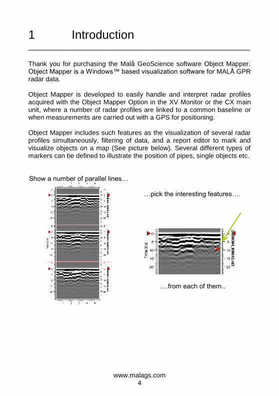
1 Introduction __________________________________________________ Thank you for purchasing the Malå GeoScience software Object Mapper. Object Mapper is a Windows™ based visualization software for MALÅ GPR radar data. Object Mapper is developed to easily handle and interpret radar profiles acquired with the Object Mapper Option in the XV Monitor or the CX main unit, where a number of radar profiles are linked to a common baseline or when measurements are carried out with a GPS for positioning. Object Mapper includes such features as the visualization of several radar profiles simultaneously, filtering of data, and a report editor to mark and visualize objects on a map (See picture below). Several different types of markers can be defined to illustrate the position of pipes, single objects etc. Show a number of parallel lines…

…pick the interesting features….

….from each of them..

www.malags.com 5

…. And instantly see the location of the mapped feature on the defined

investigation area

Object Mapper can also be used with previously acquired MALÅ GPR data profiles, as an Object Mapper project can easily be created within the Object Mapper software. The system requirements for Object Mapper are:

Windows XP or Windows 7 300MHz Pentium processor 512MB of RAM

www.malags.com 6

Malå GeoScience welcomes comments from you concerning your experience using the software, together with comments on the contents and usefulness of this manual. To help MALÅ GeoScience deal with your comments, always include the software version number. Malå GeoScience postal address is: Main Office: MALÅ GeoScience AB Skolgatan 11 S-930 70 Malå Sweden Phone: +46 953 345 50 Fax: +46 953 345 67 E-mail: sales@malags.com North & South America: China: MALÅ GeoScience USA, Inc. MALÅ GeoScience 2040 Savage Rd, P.O. Box 80430 Charleston, SC 29416 USA China Phone: +1 843 852 5021 Phone: Fax: +1 843 769 7392 E-mail: sales.usa@malags.com

Technical support issues can be sent to: support@malags.se Information about MALÅ GeoSciences products is also available on the Internet: http://www.malags.com

www.malags.com 7

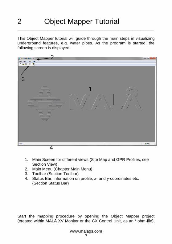
2 Object Mapper Tutorial __________________________________________________ This Object Mapper tutorial will guide through the main steps in visualizing underground features, e.g. water pipes. As the program is started, the following screen is displayed:

1. Main Screen for different views (Site Map and GPR Profiles, see Section View)

2. Main Menu (Chapter Main Menu) 3. Toolbar (Section Toolbar) 4. Status Bar, information on profile, x- and y-coordinates etc.

(Section Status Bar) Start the mapping procedure by opening the Object Mapper project (created within MALÅ XV Monitor or the CX Control Unit, as an *.obm-file),

1

2

3

4

www.malags.com 8

by pressing in the Toolbar or by using the command Open under the File menu. If using data files already acquired with Ground Vision or without the Object Mapper option in the Monitor or CX Main unit, use the command New (->

File or ) and follow the easy steps in the Project Manager (See also Section Project Manager below) to create a new Object Mapper Project.

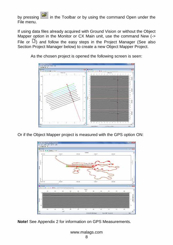
As the chosen project is opened the following screen is seen:

Or if the Object Mapper project is measured with the GPS option ON:

Note! See Appendix 2 for information on GPS Measurements.

www.malags.com 9

To the left the Site Map is displayed, with the baseline (as defined in the XV Monitor or in the Object Mapper program itself) in red (if the baseline option is used in the Monitor) and all the associated radar profiles in green, brown, blue or black. If the GPS option is used (in the Monitor) the profiles are displayed without any baseline. In the right hand screen the radargrams are shown. Selected radargram is at top. Visual part of the profile is green and hidden part of profile is brown in the Size Map. The radargrams shown below is marked with blue colour on the site map. Up to ten radargrams can be displayed simultaneously, see Section Options to find out how. The rolling wheel on the mouse can be used to scroll the radar data when the GPR Profiles window is active. To enhance the data quality, a number of different filters can be applied to the radar data. See Section Edit Filter List and Appendix 1. Furthermore, the contrast of the radargram can be adjusted with the

contrast scrollbar at the top right in the GPR Profiles

View, while the active filters also can be turned on and off by pressing . When measuring with the GPS option there are two ways of adjusting the display of the GPR profiles to make it as correct as possible. See example below, where the long profile (at right) is displayed together with two shorter ones. When right-clicking in the profile the options Directions of GPS profiles and Horizontal Alignment for GPS profiles is seen.

www.malags.com 10

Directions of GPS profiles gives you:

And Horizontal Alignment: Note! Even with GPS it is recommended to measure in parallel profiles, as this will enable to view several GPR profiles simultaneously and by that comparison of identified objects in different lines.

www.malags.com 11

When the radar data looks as desired, the interpretation of objects/features can be started. To do this, just click on some of the seven different marker

types in the GPR Profiles view . See Section Tools to explore how these are defined. After clicking on one marker type the mouse pointer changes to a cross which can be placed on an identified hyperbola in the different radargrams. See the example below, showing a blue marked object and the markers cross.

Note! The marker function is inactivated by pressing the marker type on toolbar again. Markers can also be placed by right clicking on the correct position on the radargram and then choose insert marker from the pop-up menu (see below). If a marker is activated (with left mouse click) a rectangle is seen around the marker, and it can be moved by drag-and drop and when right clicking on the marker a pop-up menu appears as seen below. Important note! The markers in the Toolbar must be inactivated; otherwise new markers will be set.

www.malags.com 12

Several markers can be marked / activated simultaneously, by keeping the “Ctrl”-button on the keyboard down. Also see information on Marker lists in Chapter 3.2.3. The Edit Marker function enables manual input of the location of the marker and change of object type. A comment can also be made, see below. The Edit Marker function is also reached by double-clicking on the marker.

To work and browse through all the files, click on the different radar profiles on the Site Map. The one clicked on will turn green and show up as the top radargram on the GPR Profiles View window. When all interesting features are identified, the project is saved and the resulting map, as shown below, can be printed immediately or exported in AutoCad dxf-format. See below. All the markers are also listed (as seen in Section Markers) and can be exported in ASCII-format with the correct position and depth. Note! The marker to be exported MUST be marked in the marker list, prior export. For more information see Section Markers 3.2.3.

www.malags.com 13

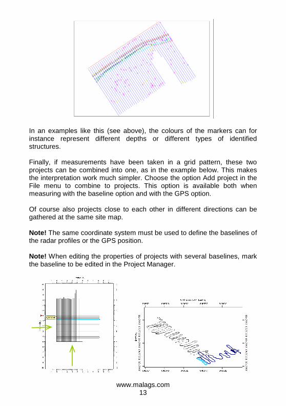
In an examples like this (see above), the colours of the markers can for instance represent different depths or different types of identified structures. Finally, if measurements have been taken in a grid pattern, these two projects can be combined into one, as in the example below. This makes the interpretation work much simpler. Choose the option Add project in the File menu to combine to projects. This option is available both when measuring with the baseline option and with the GPS option. Of course also projects close to each other in different directions can be gathered at the same site map. Note! The same coordinate system must be used to define the baselines of the radar profiles or the GPS position. Note! When editing the properties of projects with several baselines, mark the baseline to be edited in the Project Manager.

www.malags.com 14

3 Main Menu __________________________________________________ The Main Menu of Object Mapper is found on the top of the screen.

3.1 File In the File menu the Object Mapper projects can be created, opened and saved. It also contains the print functions. New: Creates a new project. See Section Project Manager below. Open: Opens an existing project. Close: Closes an opened project. Save: Saves an opened project using the same file name. Save As: Saves an opened project to a specified file name. Export: Exports the resulting map, with markers to DXF-format, markers to ASCII-format lists or to MALÅ GPS Mapper format. Note! The markers to be exported must be selected in the Markers list. Add project: Adds another project to the existing one. Print: Prints the current view. Preview: Displays the document on the screen, as it would appear printed. Print Setup: Selects a printer and printer connection. Exit: Exits the programme.

For the Export option to *.dxf, the different marker types on the map are exported to separate layers.

www.malags.com 15

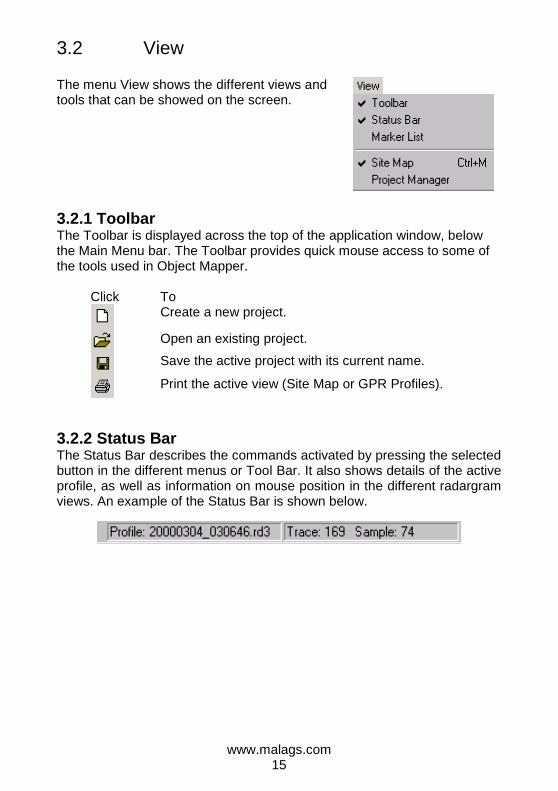
3.2 View The menu View shows the different views and tools that can be showed on the screen.

3.2.1 Toolbar The Toolbar is displayed across the top of the application window, below the Main Menu bar. The Toolbar provides quick mouse access to some of the tools used in Object Mapper. Click To

Create a new project.

Open an existing project.

Save the active project with its current name.

Print the active view (Site Map or GPR Profiles).

3.2.2 Status Bar The Status Bar describes the commands activated by pressing the selected button in the different menus or Tool Bar. It also shows details of the active profile, as well as information on mouse position in the different radargram views. An example of the Status Bar is shown below.

www.malags.com 16

3.2.3 Marker list In the marker list, all the identified and marked features are saved, according to their type and position.

By right-clicking on one of the markers, the marker can be edited or deleted. It is also possible to choose to hide or select the marker (singly, by type or all together).

With the option Export (in the Main menu) this list with selected markers can be exported to ASCII-format, where all marked objects are listed together with type, trace-, sample-, x-, y- and z-position. Note! The marker information also can be exported in DXF-format or to Malå GPS Mapper-format.

www.malags.com 17

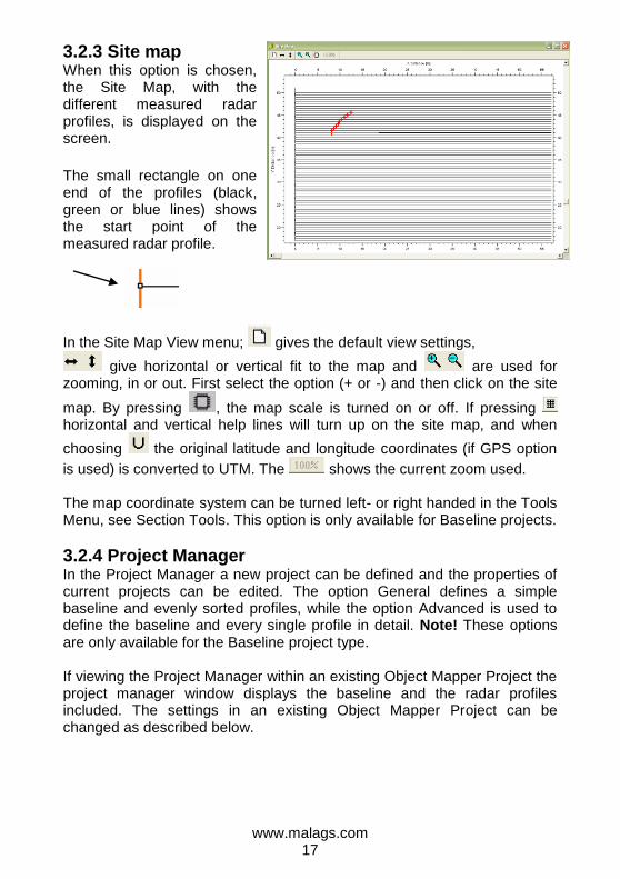
3.2.3 Site map When this option is chosen, the Site Map, with the different measured radar profiles, is displayed on the screen.

The small rectangle on one end of the profiles (black, green or blue lines) shows the start point of the measured radar profile.

In the Site Map View menu; gives the default view settings,

give horizontal or vertical fit to the map and are used for zooming, in or out. First select the option (+ or -) and then click on the site

map. By pressing , the map scale is turned on or off. If pressing horizontal and vertical help lines will turn up on the site map, and when

choosing the original latitude and longitude coordinates (if GPS option

is used) is converted to UTM. The shows the current zoom used. The map coordinate system can be turned left- or right handed in the Tools Menu, see Section Tools. This option is only available for Baseline projects.

3.2.4 Project Manager In the Project Manager a new project can be defined and the properties of current projects can be edited. The option General defines a simple baseline and evenly sorted profiles, while the option Advanced is used to define the baseline and every single profile in detail. Note! These options are only available for the Baseline project type. If viewing the Project Manager within an existing Object Mapper Project the project manager window displays the baseline and the radar profiles included. The settings in an existing Object Mapper Project can be changed as described below.

www.malags.com 18

If a new Object Mapper Project is desired (with profiles acquired with GruondVision or the Monitor but not in an OBM project), just open the Project Manager and press Add to first add a new baseline and then to add the different radar profiles belonging to that baseline. If the data is collected without baseline but with GPS, the project type is changed to GPS support and then only the option Add profiles is available.

For both project types, Baseline or GPS, the location and name of the new project is given in the top line. Note! The project should be saved at the same location as the added radar profiles are situated. The possibility to browse between different folders to find an existing project is also available. Several profiles can be added simultaneously by using “Ctrl” on the keyboard. The sequence of the radar profiles can be changed by “drag and drop” in the profiles list. If new files are added later on these are added in alphabetical order. Note! When editing the properties of projects with several baselines, mark the baseline to be edited in the Project Manager (->Advanced).

With the option the profiles can be arranged by:

www.malags.com 19

- Equal interval for all profiles - Profile direction, left or right of

the base line start (see picture below).

- Giving every second profile opposite direction.

If the option Profiles measured to the right of baseline start is chose the site map will be made as: Note! The start point of the Baseline is set to X=0 and Y=0.

If the option Profiles measured to the left of baseline start is chose the site map will be made as: Note! The start point of the Baseline is set to X=0 and Y=0.

1st 2nd

1st 2nd

www.malags.com 20

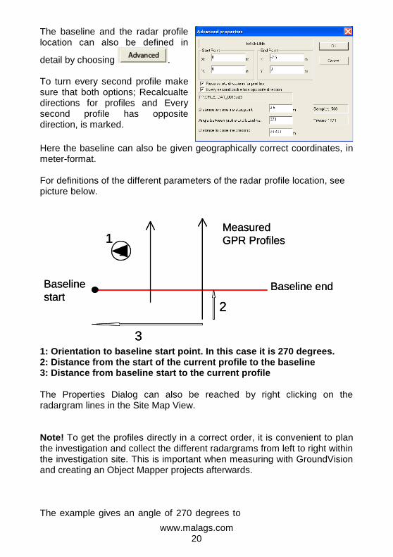
The baseline and the radar profile location can also be defined in

detail by choosing . To turn every second profile make sure that both options; Recalcualte directions for profiles and Every second profile has opposite direction, is marked.

Here the baseline can also be given geographically correct coordinates, in meter-format. For definitions of the different parameters of the radar profile location, see picture below.

1

3

1

24

Baseline end

Measured

GPR Profiles

Baseline

start

1

3

1

24

Baseline end

Measured

GPR Profiles

Baseline

start

1: Orientation to baseline start point. In this case it is 270 degrees. 2: Distance from the start of the current profile to the baseline 3: Distance from baseline start to the current profile The Properties Dialog can also be reached by right clicking on the radargram lines in the Site Map View. Note! To get the profiles directly in a correct order, it is convenient to plan the investigation and collect the different radargrams from left to right within the investigation site. This is important when measuring with GroundVision and creating an Object Mapper projects afterwards. The example gives an angle of 270 degrees to

www.malags.com 21

the baseline start point. If the profiles are measured from right to left the angle to the baseline start point should be set to 90 degrees.

Baseline start (X=0, Y=0)

3.3 Profile The Profile menu handles the colours and filters for the displayed radargrams.

3.3.1 Change Palette Change Palette opens the Palette Manager where the possibility to change the colour scheme from black/white to colour is available. The palette shows the current colours for the open radargrams. To change single colour values, just double click on them. The operator can also change a spectrum of colours, by using the command Interpolate, after having changed two colours. The command Load Palette will open previously designed and saved palettes.

1st

2nd

3rd

and so on

www.malags.com 22

3.3.2 Edit Filter List The option Set Filters under the Profile menu will open the Filter Manager. Here the operator can choose which filters and processing steps he/she wants to apply on the radar data, and also modify the settings of these.

Note! See also Appendix 1 for more information on filters.

Filters available Shows the available Object Mapper software filters. Filters applied This space will list the current filters applied to the

radar data. To edit the filters applied, mark the filter with the mouse and press Edit, or double-click.

Add Add is used to add marked filters from the Filters Available list.

Remove Press remove to take away marked filters from the Filters Applied list.

The created filter list can be saved with and used again later

by . The command Ctrl+F will disable all filters at once. And when pressing Ctrl+F again the filters are turned on.

3.4 Tools In the Tools menu the operator can change the settings of the GPR Profiles view. For instance, the operator can choose between meter and feet as measuring unit, how the coordinate system on the Site Map should be arranged, how many parallel profiles to display simultaneously and what velocity should be applied for the depth scale. Furthermore the different marker types can also be defined here. In the Dialog Options the following tabs can be found:

www.malags.com 23

General Tab

The user can chose to use the project name when the site map is printed or on own defined name. Below an example is given of the two map coordinate systems for the same project; left handed (at left below) and right handed (at right below).

Export of DXF: Option of how UTM coordinates will be set. Easting first will project all east-west values to X-axis and North-South to Y-axes. Northing first will set North-South values to X-axis and East-West values to Y axis. Both options will keep depth position at Z-axis.

www.malags.com 24

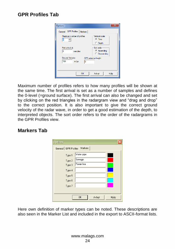
GPR Profiles Tab

Maximum number of profiles refers to how many profiles will be shown at the same time. The first arrival is set as a number of samples and defines the 0-level (=ground surface). The first arrival can also be changed and set by clicking on the red triangles in the radargram view and “drag and drop” to the correct position. It is also important to give the correct ground velocity of the radar wave, in order to get a good estimation of the depth, to interpreted objects. The sort order refers to the order of the radargrams in the GPR Profiles view.

Markers Tab

Here own definition of marker types can be noted. These descriptions are also seen in the Marker List and included in the export to ASCII-format lists.

www.malags.com 25

Appendix 1 Filters

____________________________________________________________ This appendix covers the available filters in the Object Mapper filter manager. The filters that have settings that need to be set have a dialog connected to them. This dialog can be called from the Filter Manager and is shown in each filter description. Common to all filter dialogs is the trace window that shows the filtered trace. The trace window is updated when there is a change in the filter settings.

Which filter to use is depending on the application and the quality of the radar image. A filter very useful for some applications can be useless in others. The knowledge and experience of the user often determines the time it takes to produce a useful image. A general recommendation is to start with DC filter and Gain. Below the available filters are listed and also if they are always, often, seldom or very seldom used in common GPR applications. Always used: DC-shift Often used: Delete Mean Trace, FIR, Time Gain Seldom used: Custom Gain, Moving Average, Moving Median, Threshold Very seldom used: Average, Median, AGC, Triangular FIR, HFIR

www.malags.com 26

Automatic gain control AGC This filter attempts to adjust the gain of each trace by equalizing the mean amplitudes observed in a sliding time window. A short window gives a more pronounced effect, the extreme of which would a one-sample window, which would cause all amplitudes to be equal. The other extreme would be a time window of the same length as the trace. This would have no effect on the trace. After equalization a constant multiplier is applied to the trace to make the resulting amplitudes reasonable.

Average The Average filter calculates a mean over a given number of samples and traces. The sample in the middle of the grid is replaced by the average value. This filter acts as a simple 2D-lowpass filter and gives a softer picture.

Custom Gain An amplifying filter where the gain factor is given manually for 32 different sections of the trace.

www.malags.com 27

DC-Filter There is often a constant offset in the amplitude of the registered trace, this is known as the DC level or the DC offset. This filter removes the DC component from the data. The DC component is individually calculated and removed for each trace. In the dialog the sample interval on which the DC component is calculated is specified. Values for the start and end samples can be entered in the edit boxes or by click-dragging in the trace view. The sample interval is shown as a red area in the trace view.

Delete mean trace This filter is used to remove horizontal and nearly horizontal features in the radargram by subtracting a calculated mean trace from all traces, sample by sample. Window width is number of traces.

FIR A quick band-pass filter, working with a combination of two boxcar (averaging) filters. The filter is run in two stages. First the lower frequencies are attenuated by subtracting the average in the longer boxcar from the raw data at the centre of the boxcar. Then the higher frequencies are attenuated by replacing each sample with the average calculated in the shorter boxcar. Both boxes calculate along the whole trace.

www.malags.com 28

HFIR The HFIR filter functions as the FIR filter, but the filter runs along the profile - not along the trace. The filter is a spatial band-pass filter and its effect is similar to that of the background removal filter

Median The Median filter functions as the Average filter, but instead of the mean value a median value is used. It removes spikes in the data efficiently while not blurring the image quite as much as the average filter does.

Moving average This filter takes the average as calculated by the average filter described above and subtracts it from the sample at the centre of the filter. Its effect is that of a simple 2D high-pass filter. Moving median As the Moving average filter, but with the median value instead of the average.

www.malags.com 29

Threshold All samples with a value below the threshold are set to zero.

Time-Gain Filter The Time-Gain filter applies a time-varying gain to compensate for amplitude loss due to spreading and attenuation. The trace is multiplied by a gain function combining linear and an exponential gain, with coefficients set by the user. In the Time-Gain dialog, there is one trace window and one gain window. The trace window shows a filtered trace and the gain window shows the gain function applied.

The red line in the trace window indicates the start of the filter (before this point the gain of the filter is unity). Triangular FIR The Triangular FIR filter functions as the FIR filter, but instead of using boxcar averages it uses averages in symmetrical triangular windows.

www.malags.com 30

Appendix 2 GPS measurements

____________________________________________________________ This appendix covers some important issues when using a GPS to position the GPR measurements. The Malå Geoscience Monitor or GroundVision software can be used together with GPS equipment which communicates via a 9-pin series connector or USB. The GPS must communicate with NMEA 0183 protocol with GGA sentence. For the Monitor there is also one type of USB GPS available, see the Operating Manual Monitor. The GPS equipment available today can be divided into three different types: GPS: Relatively inexpensive, the GPS is using only satellites for positioning, accuracy around ± 4 m. Suitable for large scaled layer mapping etc. DGPS: Differential GPS, uses satellites and a correction from a reference station/satellite, accuracy around ± 0.5-2 m. Similar systems are EGNOS (Europe), WAAS (USA) and MSAS (Japan). RTK GPS: Real Time Kinematic GPS, expensive, uses two GPS receivers (one stationary base and one rover) and correction signal from the base antenna, accuracy around ± 1-2 cm. Network RTK also available in many locations, where the correction is received via GSM. RTK GPS accuracy is recommended for utility mapping. For all the three different GPS systems the following is very important to remember: 1) Regardless the system used; GPS, DGPS or RTK, the positioning data gathered will be of bad quality if the measurements are made under bridges, in dense forest, close to high buildings etc. In the example below the lowermost line is measured 1 m from a building, resulting in incorrect positioning of that measurement line.

www.malags.com 31

2) When using a GPS in motion, the GPS system is updated more or less seldom. Inexpensive systems may update 1 time/second while RTK systems can update 10 or more times/second. 3) The GPS antenna should be placed on the middle of the GPS antenna to give the most correct position of the GPR traces. This will be a problem when measuring with the Malå Geoscience RT antennas, and should be corrected afterwards.

4) It should be observed that during the day the connection to satellites can change, giving better or worse positioning possibilities.

www.malags.com 32

Appendix 3 Software license

____________________________________________________________

After installation of software, a time limit license will be set for

evaluation period.

When this time has expire user must buy the software for future use.

Object Mapper has two types of licenses, node license and hardware

license.

Node license is a license locked to one specific computer.

Hardware license is license stored on a special USB device (called

USB dongle). This type of license can be used on any computer with

this software installed.

Contact Malå Geosciences how to acquire a new license / hardware

key.

www.malags.com 33

Get identification Open license dialog window from menu Tools License Manager

Dependent on what license type you require you need you have to copy

information from one of two groups, USB Dongle or Node license.

USB Dongle license Make sure you have inserted USB dongle before you open this window.

Use the button “Copy to clipboard” when you copy the information. You can then

paste it into your e-mail (use the menu ‘edit’ ’paste’ or key CTRL + V in your e-

mail program).

If you don’t have a USB dongle it will be sent to you by MALÅ Geoscience with

a license.

Node license When you order a node license, you need to send computer ID and license ID.

It is recommended to use the button “Copy to clipboard” when you copy the

information.

Hardware license information

Node license information

Current license

information

Source of current

license information

www.malags.com 34

Set license information

Hardware key

If you have a USB dongle you will receive an exe file. Run this file with the USB

dongle inserted and license will be written to dongle.

Start Object Mapper.

Node license You need to open license dialog window. Use the button Open license file to read

.lic file you have received.