Nuremberg Institute of Technology -...

Nuremberg Institute of Technology

Faculty of Electrical Engineering, Precision Engineering

and Information Technology

Study Programme

Media Engineering

Bachelor Thesis

submitted by

Patrick Werner

Integration of Light Field Data in

a Computer Generated 3D

Environment

Winter Semester 2016/2017

supervised by

Prof. Dr. Matthias Hopf

Prof. Dr. Stefan Röttger

Dipl. Ing. Matthias ZieglerFraunhofer IIS

Keywords: light field, virtual reality, 3D, computer graphics

Plagiarism Declaration in Accordance with Examination Rules

I herewith declare that I worked on this thesis independently. Furthermore, it was not

submitted to any other examining committee. All sources and aids used in this thesis,

including literal and analogous citations, have been identified.

Signature

Foreword

I would like to thank everybody that helped and supported me during the creation of this

thesis. Especially my supervisor at Fraunhofer IIS Dipl. Ing. Matthias Ziegler, who advised

me throughout this work. Additionally I would like to thank the group CIA which enabled

this thesis and gave me an opportunity to display my work at a convention. Finally I

thank my supervising professors Dr. Matthias Hopf and Dr. Stefan Röttger.

Contents

Acronyms 5

1. Introduction 6

1.1. State-of-the-art . . . . . . . . . . . . . . . . . . . . . . . . . . . . . . . . . 71.2. Motivation . . . . . . . . . . . . . . . . . . . . . . . . . . . . . . . . . . . . 71.3. Overview . . . . . . . . . . . . . . . . . . . . . . . . . . . . . . . . . . . . . 8

2. Basics 9

2.1. Light field . . . . . . . . . . . . . . . . . . . . . . . . . . . . . . . . . . . . 92.1.1. Capturing methods . . . . . . . . . . . . . . . . . . . . . . . . . . . . 102.1.2. Workflow . . . . . . . . . . . . . . . . . . . . . . . . . . . . . . . . . 122.1.3. Depth image based rendering . . . . . . . . . . . . . . . . . . . . . . 15

2.2. 3D computer graphics . . . . . . . . . . . . . . . . . . . . . . . . . . . . . . 172.2.1. Modelling . . . . . . . . . . . . . . . . . . . . . . . . . . . . . . . . 172.2.2. Rendering . . . . . . . . . . . . . . . . . . . . . . . . . . . . . . . . 192.2.3. Graphics pipeline . . . . . . . . . . . . . . . . . . . . . . . . . . . . . 21

2.3. Virtual reality . . . . . . . . . . . . . . . . . . . . . . . . . . . . . . . . . . 222.4. Digital video . . . . . . . . . . . . . . . . . . . . . . . . . . . . . . . . . . . 22

2.4.1. Codec . . . . . . . . . . . . . . . . . . . . . . . . . . . . . . . . . . 23

3. Theory 24

3.1. Transforming the CG coordinates . . . . . . . . . . . . . . . . . . . . . . . . 253.2. Intersection with the light field canvas . . . . . . . . . . . . . . . . . . . . . 263.3. Calculation of the perceived position . . . . . . . . . . . . . . . . . . . . . . 28

4. Implementation in the Unreal Engine 29

4.1. General information about the Unreal Engine . . . . . . . . . . . . . . . . . . 294.1.1. Actor . . . . . . . . . . . . . . . . . . . . . . . . . . . . . . . . . . . 304.1.2. Graphics Programming . . . . . . . . . . . . . . . . . . . . . . . . . . 304.1.3. Plugins . . . . . . . . . . . . . . . . . . . . . . . . . . . . . . . . . . 304.1.4. Media Framework . . . . . . . . . . . . . . . . . . . . . . . . . . . . 314.1.5. Blueprints . . . . . . . . . . . . . . . . . . . . . . . . . . . . . . . . 31

4.2. Architecture . . . . . . . . . . . . . . . . . . . . . . . . . . . . . . . . . . . 324.3. FViewrenderer plugin . . . . . . . . . . . . . . . . . . . . . . . . . . . . . . . 32

4.3.1. Compute shader implementation: FForwardWarpDeclaration . . . . . . 334.3.2. Quality improvements . . . . . . . . . . . . . . . . . . . . . . . . . . 34

4.4. ALightfieldActor . . . . . . . . . . . . . . . . . . . . . . . . . . . . . . . . . 364.4.1. C++ . . . . . . . . . . . . . . . . . . . . . . . . . . . . . . . . . . . 364.4.2. Blueprint . . . . . . . . . . . . . . . . . . . . . . . . . . . . . . . . . 374.4.3. LightfieldMaterial . . . . . . . . . . . . . . . . . . . . . . . . . . . . 37

4.5. Embedding of video data . . . . . . . . . . . . . . . . . . . . . . . . . . . . 374.5.1. High resolution . . . . . . . . . . . . . . . . . . . . . . . . . . . . . . 384.5.2. High frame rate . . . . . . . . . . . . . . . . . . . . . . . . . . . . . 39

4.5.3. Quality improvements . . . . . . . . . . . . . . . . . . . . . . . . . . 404.6. Preparation for CES . . . . . . . . . . . . . . . . . . . . . . . . . . . . . . . 40

5. Evaluation 43

5.1. Comparison with a 3D object . . . . . . . . . . . . . . . . . . . . . . . . . . 435.2. Impact of video compression . . . . . . . . . . . . . . . . . . . . . . . . . . . 465.3. Performance . . . . . . . . . . . . . . . . . . . . . . . . . . . . . . . . . . . 465.4. User feedback . . . . . . . . . . . . . . . . . . . . . . . . . . . . . . . . . . 47

6. Conclusion 48

6.1. Outlook . . . . . . . . . . . . . . . . . . . . . . . . . . . . . . . . . . . . . 48

Bibliography 49

Appendices

A. Blueprints 52

B. Code Listings of public members 58

C. List of Figures 60

D. List of Tables 62

E. List of Listings 63

Acronyms

xD x dimensional

UHD 3840 × 2160 resolution

API application programming interface

CES Consumer Electronics Show

CIA Computational Imaging and Algorithms

CG computer generated

CPU central processing unit

CRF constant rate factor

D6 six-sided die

D8 eight-sided die

DIBR depth image based rendering

FOV field of view

FHD 1920 × 1080 resolution

HMD head mounted display

IIS Institute for Integrated Circuits

GPU graphics processing unit

MSE mean squared error

PNG Portable Network Graphics

RGB red, green, blue

RHI rendering hardware interface

VR virtual reality

YCbCr luminance, blue-yellow chrominance, red-green chrominance

1. Introduction

1. Introduction

“Virtual Reality refers to immersive, interactive, multi-sensory, viewer-centered,

three-dimensional computer generated environments and the combination of

technologies required to build these environments”

— Carolina Cruz-Neira,SIGGRAPH ’93 Course Notes “Virtual Reality Overview” No. 23, pp. 1.1 - 1.18 (1993)

“Virtual Reality refers to the use of three-dimensional display and interaction

devices to explore real-time computer-generated environments.”

— Steve BrysonCall for Participation 1993 IEEE Symposium on Research Frontiers in Virtual Reality

Virtual reality (VR) has come a long way since the beginnings in 1962, when the Sensorama

first introduced multi-modal experiences with scent cards, wind and vibrations [12], albeit

still lacking interactivity. This was fixed by “The Sword of Damocles”, it featured the first

head mounted display (HMD) with positional and orientational tracking [30]. Nowadays

access to the virtual reality is even purchasable by consumers, with the HTC Vive, Oculus

Rift or Playstation VR.

With this breakthrough into the consumer world, new technologies regarding VR gain in

importance. There are several approaches to combine the reality with virtual reality, with

so called mixed or augmented reality applications. Augmented reality strives to improve

experiences for the user through additional virtual objects in the real world, projected

through a HMD [2]. Another approach would be improving computer generated worlds

with real objects. 3 dimensional (3D) reconstruction is possible through 3D scanning or

photogrammetry, however these technologies are mostly limited to static objects [18]. A

different way to reconstruct 3D data is through computer vision, here the results are purely

based on the captured data.

One computer vision approach is through light fields, which capture the light flow of a

scene in multiple directions. Light fields can be created by capturing a high amount of

viewpoints of the same scene, e.g. by a plenoptic approach like the consumer camera

Lytro Illum [16], the newer Lytro Immerge [17] or camera arrays as proposed by Stanford

University [31]. While Stanford University used dense camera arrays to capture light fields

the Fraunhofer Institute for Integrated Circuits (IIS) acquires light field data by capturing

with sparse arrays. Through using less cameras and therefore lowering the amount of

created data, processing times can be improved.

This type of footage allows for multiple new post processing effects, like the selection of a

new focal point with synthetic aperture or light field rendering. It allows the selection of

an arbitrary view point inside the light field bounds, for which a virtual camera view can

be computed.

Patrick Werner 6 of 63

1. Introduction

On the basis of this light field rendering, an approach that brings light field data into a

computer generated (CG) world seems plausible.

1.1. State-of-the-art

The current capturing methods to create 3D objects were briefly touched in the Introduction

1. Another possible solution would be modelling by hand, this however requires a master

of his craft to accurately represent the real object. The disadvantage in most of these is

the limitation to static objects, or the massively increased effort needed to capture video

data.

There are also different ways to represent real objects in 3D. Most capturing techniques

supply depth data, this data can be used to generate point clouds. However, these are

often hard to represent, because of the high amount of points necessary to completely fill

the object. Another way is to generate mesh data, either directly from the captured data,

or by surface reconstruction from point clouds. Though the accuracy is often limited and

movement is not easily translated into animations.

1.2. Motivation

With the rising popularity of VR and the logical connection to light field data, a real time

light field renderer has been developed at Fraunhofer IIS’ group Computational Imaging

and Algorithms (CIA). This renderer works through shaders on the graphics processing

unit (GPU), it encompasses a full depth image based rendering (DIBR) process.

The goal of this thesis is to combine the real time light field renderer with a CG environment,

enabling convincing light field data inside of a 3D world. From the given basics a new

projection model should be derived, that produces correct positions for the light field

rendering. Furthermore, this model, together with the shaders, should be implemented

into a CG environment. At first the light field itself should be integrated, but a special

focus lies on the addition of light field video data. This may lead to highly immersive

applications improved by live action footage. The result should be a demonstrator proving

the seamless connection of light fields and CG.

During the course of this thesis, group CIA decided that the resulting demonstrator should

be presented at the Consumer Electronics Show (CES) 2017 in Las Vegas. Considering

this, additional content was created, which should be highlighted with small interactive

elements.


1. Introduction

Light

field

Virtual

reality

3D computer

graphics

Basics

Thesis

Implementation

Theory

Demonstrator

Projection

model

Unreal

Engine

Fraunhofer

IIS shaders

Content

Prerequisites

Figure 1.1.: Overview of this thesis

1.3. Overview

In chapter 2 the necessary foundations for this thesis will be explained, starting with light

field technology, how a light field is captured and converted into usable disparity maps.

Following that, the basics of 3D computer graphics are described, firstly the modelling

process, secondly how rendering works and finally the graphics pipeline executed on the

GPU. Afterwards, virtual reality and digital video are briefly introduced.

The following chapter 3 describes the theory behind the connection of the light field to

the CG world. Here the individually taken steps, as well as their formulas are covered.

Continuing in chapter 4, the chosen 3D environment, the Unreal Engine is described.

Followed by an insight into the implementation. Starting with the FViewrenderer plugin,

a compute shader that produces viewrendered images given the appropriate input data.

Then the ALightfieldActor, the canvas that the resulting image gets drawn on, and the

methods to get light field video data into the engine are explained.

Next, the results are evaluated in chapter 5. In this chapter the effects of chapter 3 on

the rendering algorithms are described using a 3D object. Furthermore, the impact of

video compression on the rendering quality is illustrated. Then the necessary settings for

a smooth performance are described. Additionally, subjective feedback of colleagues is

assessed.

Finally the work is summarized in chapter 6 and an outlook explores future possibilities.


2. Basics

2. Basics

In this chapter the foundations needed for this bachelor thesis are described and illustrated.

Starting with the introduction to light field technology, different kinds of capturing methods

are demonstrated. Next the light field processing workflow used at Fraunhofer IIS, as well

as the light field rendering are described.

This is followed by an explanation of 3D computer graphics and vector spaces. Finally the

concepts of virtual reality and digital video are briefly touched.

2.1. Light field

Figure 2.1.: An eye gathering light rays

A theoretical light field contains all information about the flow of light in a 3D space,

as depicted in figure 2.1. The radiance, as well as the direction of every light ray inside

that space is known, this is represented in the 5D plenoptic function [1]. As this function

contains redundant information (outside of the bounds of convex objects) it can be reduced

to a 4D function [21]. This can be captured by a digital camera, given multiple viewpoints

of the same scene, as such a “light field can be interpreted as a 2D collection of 2D images,

each taken from a different observer position.” [21]

By photographically capturing an object with multiple varying viewpoints, the 4D light

field is created. With this light field data, multiple computer generated effects can be

realised. One of them is synthetic aperture, it allows refocusing after the picture is already

taken. This is also featured by the consumer light field camera Lytro Illum [16]. Another

possibility is view rendering, also called light field rendering [22], which allows rendering

of virtual camera positions across the light field.


2. Basics

2.1.1. Capturing methods

There are several approaches to capturing light field data, which are described in the

following sections. Dedicated plenoptic cameras, camera arrays or gantry systems are

possible. All working on the same principle of capturing a scene from multiple different

viewpoints.

Robotic linear axis

Figure 2.2.: Line gantry at Fraunhofer IIS

One of the first systems for capturing light fields used a moving camera, which periodically

took pictures from different viewpoints [22]. This is achievable through manual camera

dollies used in film making or motorized gantries. A gantry, normally used in manufacturing,

can be programmed to capture the light field as desired. With this capturing method a

high amount of samples can be created for the light field, with the disadvantage of only

allowing static objects.

At Fraunhofer IIS a 2D gantry with a high quality camera is used to capture planar light

fields, shown in figure 2.2. It has 4.0 meters horizontal and 0.5 meters vertical freedom of

movement.

Plenoptic cameras

Because a gantry is not very convenient, another way to capture light field data is through a

plenoptic camera. The Lytro Illum [16] provides access to light field capturing to consumers.

Figure 2.3.: The Lytro Illum plenoptic camera [16]


2. Basics

Plenoptic cameras work by capturing a dense light field through a micro-lens array inside

of the hand held device [25]. These spread the light rays coming through the main lens into

micro images captured by the camera sensor. As a result, this enables the aforementioned

synthetic aperture after the shooting of the scene itself, through plenoptic image processing

[25]. However, this method of capturing is limited by the narrow perspective, which does

not enable effects based on the geometry of the scene. Similar to the gantry, these consumer

cameras currently only work for still images, but Lytro currently has a plenoptic video

camera for rent [15]. Additionally Lytro offers a prototype of a 360° light field camera,

that can also capture moving scenes [17].

Camera arrays

Figure 2.4.: Black magic 3 × 3 camera array

To overcome some of the limitations of the robotic approach and plenoptic cameras, one of

the first, inexpensive to produce, dense camera arrays was suggested by Stanford University

in 2005 [31].

Multi camera arrays benefit from the modular setup possibilities. With the simplest setup

being planar, which allows high resolution, high dynamic range video, or even virtual dolly

shots [31].

By diverting from the densely packed array to a more spaced out one, the available range of

motion for geometry based effects is increased, while keeping the data rates manageable.

Other possible setups include a 360° rig [13], convex or concave placements. Even arbitrarily

placed cameras are researched [34].

Of course, the cameras need to have matching intrinsic parameters. For video purposes

these cameras also need to be synchronizable.

Fraunhofer IIS group CIA has different types of planar arrays available, with the most

recent one being a 3840 × 2160 resolution (UHD) supporting 3 × 3 array with Studio 4K

Blackmagic devices, shown in figure 2.4.


2. Basics

Image

AcquisitionImage

Rectification

Greenscreen

Keying

Disparity

Estimation

Disparity

Post-processing

Depth Image

Based Rendering

Figure 2.5.: The Fraunhofer IIS light field rendering workflow

2.1.2. Workflow

As a consequence of using sparse camera arrays direct light field rendering does not work.

By creating disparity maps from the sparse camera array images, a denser light field can

be reconstructed [19]. This is sufficient for several post production effects [32].

One such approach is presented by Foessel et al. in [9] as well as by Zilly et al. in [33] and

consists of 4 essential steps, cf. figure 2.5.

In the following this approach is described in detail on a data set created by the previously

mentioned line gantry. The subject is a Cleopatra figurine, which is placed in front of a

green screen. It was sampled simulating a 21 × 11 camera array, one image is shown in

figure 2.6.

Figure 2.6.: The Cleopatra object captured

Image rectification

In order to simplify the following step of disparity estimation the images have to be rectified.

Although the cameras in an array are mounted with high precision, small imperfections

cause corresponding pixels to be misaligned.

Rectification tries to adjust the images so that the corresponding pixels can be found in

the same row or column in every neighbouring image, cf. figure 2.7.


2. Basics

Figure 2.7.: Rectified images of the Cleopatra figurine. The rectangle shows the alignedpixels.

Green screen keying

Now the images may be keyed in order to remove the green screen. This removes unnecessary

areas beforehand, as these may negatively affect the following steps.

Disparity estimation

With the source material rectified, the next step can be approached. In order to create

appropriate disparity maps, several intermediate steps are needed. To ease complexity, the

following step is illustrated on a stereo pair of the Cleopatra data set. The same principles

can be extended for use in a multi image setup.

Disparity describes the distance in pixels between two corresponding pixels of neighbouring

images. E.g. the cat ear in figure 2.6 can be found x pixels shifted to the right in its

left adjacent image, as can be seen in figure 2.8. Ideally a disparity map contains this

information for every pixel of an image, which provides implicit geometric information

about the scene.

There are several different disparity estimation algorithms, with different strengths and

weaknesses [28][27]. Even real time disparity estimation is possible, e.g. with multi image

correspondences [6].


2. Basics

Figure 2.8.: Disparity estimation of the cat ear. The ear can be found in the adjacentimage shifted by the disparity.

Commonly 3D CG software supplies depth data in form of depth maps. These describe

the distance of each pixel to the camera based on the rendering range. Depth maps can be

calculated from disparity maps using the equation

ρ =B · f

δ · du

(2.1)

where ρ describes the depth, B the baseline, f the focal length, δ the disparity and du the

width of one pixel on the image sensor.

Because the viewpoints differ in perspective, not all disparities can be found through image

based algorithms. These occlusions can be significantly reduced in the multi camera case

by merging the disparity maps of all available views.

Disparity post-processing

As most algorithms have problems in areas with low fidelity or uniform surfaces wrong or

no disparities may be produced. Most of the erroneous disparities can be sorted out by cross

checking with neighbouring images for differing values, through so called consistency checks.

Then the missing disparities may be filled with surrounding values through filtering.

(a) Raw disparity map (b) Post processed disparity map

Figure 2.9.: Comparison of disparity post-processing outcome


2. Basics

In the end a fully filled disparity map without errors, shown in figure 2.9, is desired, as

subsequent effects quality correlates with the disparity maps quality.

Because disparity maps contain floating point data, the images are saved in a specific

way. Formats that can handle floating point data are often not fully supported, as a work

around the single channel data is split into 8 bit red, green, blue (RGB)1 data, with each

channel containing special information. Each value of red represents a disparity of 256,

green contains the range between 1 and 256 and finally blue saves the fractional digits.

This representation can be saved in many highly supported formats, e.g. Portable Network

Graphics (PNG). However, in the context of this thesis the disparity maps are converted

to a coloured representation, highlighting the full disparity range.

2.1.3. Depth image based rendering

One of the possible effects is the free viewpoint rendering. An arbitrary position inside the

light field can be chosen and a virtual camera view from that position will be rendered.

This is achieved through multiple steps that build on top of each other.

A virtual image is created by warping a set amount of surrounding images to that position

and then merging the results. The warping is split into the forward and backward warping,

which happens for every viewpoint individually. Then these warped images are combined

in the merge process [26][8][7].

Real

Camera

Real

Camera

Real

Camera

Real

Camera

Virtual

Camera

Figure 2.10.: Viewrendering in a 2 × 2 array

As an example a 2 × 2 subset of the Cleopatra data set is used. In order to exaggerate

the effect a higher baseline distance was chosen. The virtual camera is positioned in the

centre, cf. figure 2.10.

Forward warp

At first every pixel in the disparity map is shifted by its disparity value d, based on the

virtual camera position CA. CA is the position between the cameras, as shown in figure

2.10, relative to the real camera position that is currently warped.

1additive colour space based on the trichromatic colour vision theory


2. Basics

This results in a shifted pixel position ~pLF for each of the disparity values, based on their

original pixel position described by u and v, cf. figure 2.11. Supplementary, the forward

warped disparity maps may be filtered to decrease rendering artefacts.

~pLF =

u

v

1

+ dCA (2.2)

(a) Incoming disparity (b) Forward warped disparity

Figure 2.11.: Forward warping

Backward warp

Next, these forward warped disparity maps are used to map the RGB values back onto

those pixels, interpolating when needed, cf. figure 2.12.

(a) Incoming image (b) Backward warped image

Figure 2.12.: Backward warping

Merge

After these steps have been performed for all available views, they are combined based on

different factors, like disparity or distance, to form the new virtual camera view, shown in

figure 2.13.


2. Basics

Figure 2.13.: Merged colour image

In the end the pixels that could not be found in any view may be filled by an inpainting

algorithm [3], that fills the missing pixels with surrounding colours.

2.2. 3D computer graphics

Another important topic is 3D computer graphics in general. It consists of multiple

subcategories, whose most important ones will be described in the following sections.

2.2.1. Modelling

At first, the 3D objects have to be created, with the most common method being modelling

by hand. Other methods may include 3D scanning or procedural generation.

As an accurate reproduction of the real world, with objects consisting of trillions of atoms,

would be infeasable, objects are approximated by their hull. These hulls consist of multiple

3D points, also called vertices. Two vertices connecting to each other form edges, multiple

form faces.

E.g. a die with perfectly flat sides can be described with 8 vertices connected by 12 edges,

which form 6 polygonal or 12 triangular faces.

Each of these primitives can also have additional attributes, like colour, normals or texture

coordinates. Colour is used for the albedo of the rendered objects, additionally normals or

texture coordinates can be used for advanced effects like lighting or texturing.

Point clouds

Point clouds are a special kind of model, consisting only of vertices. These are most often

the result of 3D scanning or reconstruction techniques, that do not provide fully conclusive

information of the objects.


2. Basics

Vector spaces

Every vertex of a model an artist creates is relative to the models origin, this is called

the model space. Every model has its own origin and respectively its own model space.

In order to combine different models, e.g. placing a die on a table, they have to be in a

common vector space, most often referred to as world space.

There always has to be an active space, to which origin the standard transformations will

be applied. E.g. there are two dice, one six-sided die (D6) one eight-sided die (D8), in

order to combine these two, a world space has to be defined. The D8 is placed inside the

D6 space, translated 10 units along the x axis. Then the world space is rotated by 90°

around the y axis. This results in the D8’s rotation being relative to the D6 origin, not its

own, as can be seen in figure 2.14.

Figure 2.14.: Dice before (left) and after (right) the rotation around the y axis

All these transformations can be described by a 4 × 4 homogeneous transformation matrix~MM , consisting of the translation matrix, the scale matrix and the 3 rotation matrices,

which describe the rotation around the respective axis, cf. equation 2.3.

~T =

1 0 0 Tx

0 1 0 Ty

0 0 1 Tz

0 0 0 1

~S =

Sx 0 0 0

0 Sy 0 0

0 0 Sz 0

0 0 0 1

~Rx =

1 0 0 0

0 cos(θ) −sin(θ) 0

0 sin(θ) cos(θ) 0

0 0 0 1

~Ry =

cos(θ) 0 sin(θ) 0

0 1 0 0

−sin(θ) 0 cos(θ) 0

0 0 0 1

~Rz =

cos(θ) −sin(θ) 0 0

sin(θ) cos(θ) 0 0

0 0 1 0

0 0 0 1

(2.3)

These transformations are combined by multiplication, creating ~MM which describes a

model’s position and orientation in its entirety. As matrix multiplication is not commutative,

and column vectors are used, transformations are read from right to left.


2. Basics

E.g. the D8 described before can only be correctly represented, if the transformations are

in the right order, as can be seen in equation 2.4.

~MMright= ~Ry

~T =

0 0 1 0

0 1 0 0

−1 0 0 −10

0 0 0 1

~MMwrong= ~T ~Ry =

0 0 1 10

0 1 0 0

−1 0 0 0

0 0 0 1

(2.4)

In order to reverse a transformation the inverse matrix of that transformation can be

multiplied to its current transformation matrix.

2.2.2. Rendering

Now that the models are in their 3D scene, their usual purpose is to be projected to a

screen. For this, a virtual camera in the 3D scene is necessary, which is usually described

by its position ~cVCG, viewing direction ~g and up vector ~t. The following section is based on

Fundamentals of Computer Graphics [29].

Figure 2.15.: Camera with up(y), forward(-z) and right(x) vector

As an intermediate step the scene is transformed into view space to simplifiy a lot of the

following maths. In view space the camera position is the origin and the camera viewing

direction correlates with one of the axes. The result can be seen in figure 2.16.

The matrix is calculated using the intermediate variables ~w, ~u and ~v based on the camera.

~w = −~g

‖~g‖

~u =~t × ~w

‖~t × ~w‖

~v = ~w × ~u

(2.5)


2. Basics

Figure 2.16.: View transformation

~MV =

ux uy uz 0

vx vy vz 0

wx wy wz 0

0 0 0 1

1 0 0 −cVCGx

0 1 0 −cVCGy

0 0 1 −cVCGz

0 0 0 1

(2.6)

Now the scene must be projected to the virtual camera’s sensor. In order to project the scene,

the last transformation, to projection space must be applied. The needed transformation

matrix depends on the type of projection, either orthographic or perspective. The additional

frustum parameters near plane n and far plane f are needed, these describe the depth of

the 3D scene that should be projected. For both projections the width nx and height ny of

the projection screen are needed.

~MPOrth=

2nx

0 0 0

0 2ny

0 0

0 0 − 2f−n

f+n

f−n

0 0 0 1

(2.7)

Beyond these the perspective projection needs the vertical field of view (FOV) φ of the

virtual camera.

~MPP ersp=

ny

nxcot φ

20 0 0

0 cot φ

20 0

0 0 f+n

n−f

2fn

f−n

0 0 1 0

(2.8)

These transformations can be combined into a Model View Projection matrix ~MMV P ,

which can subsequently be used to fully transform and project a model.


2. Basics

2.2.3. Graphics pipeline

Modern GPUs have a programmable graphics pipeline, one example is depicted in figure

2.17. It consists of the steps to create a 2D pixel image from a 3D scene.

Prior to the GPU processing, the 3D software prepares the models and calculates their

accompanying ~MMV P . These are then send to the GPU for rendering.

Figure 2.17.: OpenGL ren-dering pipeline [14]

Basically, the standard pipeline has two main programmable

components, the vertex or geometry shader and the fragment

or pixel shader.

At first the vertex shader is called for every vertex in the

object, here the ~MMV P is applied to the vertex in order to

transform and project it. Also other geometry based effects

can be applied here, like vertex based lighting.

In the next step these vertices go through post-processing.

Vertices outside of the view frustum are removed by the

clipping.

Afterwards, the primitives are assembled out of the left over

vertices. Primitives not meeting specific criteria, like facing

the camera, can then be removed, this is also called culling.

Next, the triangle primitives are rasterized into fragments.

These contain interpolated data of the surrounding vertices.

Now, in the fragment shader effects can be applied to each

fragment individually such as per-fragment-lighting or tex-

turing.

At last, the fragments run through different tests which determine their visibility, e.g. for

overlapping fragments, the nearest to the camera wins. Additionally, the fragments may

be blended using alpha values. Finally, the coloured pixel is generated as output.

More modern graphics cards also support compute shaders. These can manipulate data

directly in a programmable environment similar to the fragment shader. Overhead is saved

by not executing the now unnecessary intermediate steps.

Rasterization rendering can also be interpreted as each pixel of the resulting image sending

out one ray. This ray transfers the colour of the first hit object, together with possible

lighting computations, back to the pixel. Similar to the way pinhole cameras work. The

back side is the image and the pinhole is comparable to the virtual CG camera. Instead of

light rays coming into the box, they are sent out from the box, cf. figure 2.18. However,

this does not compare to full ray tracing rendering methods, as these aim to realistically

replicate light rays bouncing off of surfaces.


2. Basics

Pinhole

camera

CG camera

Light rays

Image

Figure 2.18.: Comparison between pinhole camera and rasterization rendering

2.3. Virtual reality

Consumer VR started with Nintendo’s Virtual boy as a failure, because of a lack colour

fidelity as well as the uncomfortable position [4]. But with current HMDs, like the Oculus

Rift or HTC Vive for the PC market, as well as Gear VR or Google Cardboard for mobile,

these limitations have mostly been lifted.

A modern HMD features at least 1920 × 1080 resolution (FHD) across its two screens with

a refresh rate of about 90Hz, which is necessary for a simulation sickness free experience.

These HMDs have inbuilt accelerometers as well as gyroscopes for rotational tracking and

the PC or console variants external tracking devices for positional tracking. With specific

optical design a large FOV is achieved. As this leads to pincushion distorted images, the

rendered images have to be barrel distorted in order to appear correct to the viewer. With

these prerequisites and suitable controllers, this can be highly immersive.

As an addition to the standard 3D CG workflow, VR adds a few extra steps. The 3D

application can access new information based on the HMD, such as position or rotation,

and use these as a basis for the camera position and orientation. It also has to render

one image for each eye, to enable a stereoscopic impression for the viewer. In the end a

compositor, provided by the HMD application programming interface (API), applies the

barrel distortion, as well as other VR specific effects.

2.4. Digital video

A digital raster image consists of columns and rows of pixels, which can contain variable

information usually RGB, optionally alpha. These so called colour channels can have a

different amount of bits representing the value, e.g. an 8 bit single channel image allows

for 256 distinct colour values. This means a 500 x 500 single channel image has a size of

250,000 bytes (about 244 kB).

This is extended in digital video, where videos basically consist of a multitude of raster

images behind each other. A single image is now called a frame. As a result a four second


2. Basics

video with 25 frames per second accounts to 25,000,000 bytes, this brings up a problem of

digital video: file size.

Albeit traditional video has many attributes that can be exploited to reduce file size.

2.4.1. Codec

In general a codec is a process to encode and decode data streams. In this process it

enables encryption or compression, which can be lossy or lossless. For media streams both

of these come into use.

One of the simpler concepts of compression for video data is to only save the full image

data for every n-th frame and the frames in between are just described by differences to

the last frame. This significantly reduces the file size.

Another differentiation to be made is lossless versus visually lossless. The human eye does

not accurately collect visual information, because the photoreceptors in the eye gather more

data from the colour green. This is a result of its high amount of luminosity information.

Truly lossless codecs support a total reconstruction of the input single frame data. However,

visually lossless codecs leave out information that cannot be seen or distinguished by the

human eye.

This is also represented in the luminance, blue-yellow chrominance, red-green chrominance

(YCbCr)2 colour model. This model differentiates from the RGB models, as it does not

represent colour, but luminosity and chrominance.

One example of a visually lossless codec, and one of the current industry standards, is

H.264 a part of the MPEG-4 standard. Its main use is the compression of high definition

video data for streaming to the internet, CD, video telephony and broadcasting. With an

extension it also supports multi view coding, which can be used for light field data, cf. [20].

However, these extended features are currently not widely supported. Additionally, special

light field codecs are researched [5], and multi view support is directly implemented in the

H.264 successor H.265 [24].

2colour space used in digital television


3. Theory

3. Theory

In order to integrate light field data seamlessly into a 3D world the light field canvas has

to have the same behaviour as standard 3D objects. These objects are basically rendered

like the pinhole camera described in figure 2.18. Because the virtual camera in light field

rendering is changing its position, the captured objects move in the resulting renderings,

as can be seen in figure 3.1. The amount of movement scales with the disparity.

Resulting renderings

R V R R RV

Figure 3.1.: Resulting object movement when rendering virtual camera views (V) betweenreal cameras (R)

Resulting is a incorrectly perceived position for the light field data in the CG scene. A

solution to this problem is provided in this chapter. To correctly render the light field data

based on the viewer position, full 3D rendering would be required. However, the real time

shaders of group CIA currently only support 2D rendering. Therefore, the following is a

2D approximation, that will be applied to the 2D rendering.

The CG scene consists of a wall with an opening where the light field canvas is placed,

various CG objects may be placed in the scene, cf. figure 3.2.

In order to compensate for the movement, the standard forward warping formula 2.2 has to

be modified. For that reason the global offset dw is introduced. It is based on the position

of the CG camera relative to the light field canvas.

Furthermore, as the light field should be integrated in a VR environment with two

viewpoints the problem of stereoscopic convergence arises. When the two cameras are

parallel the image is perceived as in front of the canvas. This however goes against the

desired effect. A solution is provided through horizontal image translation represented

in the additional offset dconv, based on the eye distance dIP D. dconv is used to shift the

stereoscopic convergence point onto the object.


3. Theory

CG camera

Canvas

CG objects

0

Figure 3.2.: Top down view of the 3D scene

With these two additional parameters the modified formulas 3.1 are developed. These

represent the left L and right R views to be rendered, respectively.

~pLFL=

uL

vL

1

+ d~cAL+

12dconvx

12dconvy

0

+

dwx

dwy

0

~pLFR=

uR

vR

1

+ d~cAR−

12dconvx

12dconvy

0

+

dwx

dwy

0

(3.1)

3.1. Transforming the CG coordinates

At first, the CG viewer camera position ~cVCGis given, this camera also has the right vector

~rCG, which is perpendicular to its viewing and up direction, as shown as x axis in figure

2.15. Additionally, the interpupillary distance dIP DCGis available.

Because the following calculations depend on the origin point being in the middle of the

canvas, all these variables have to be converted to their counterpart in the model space of

the light field canvas, by multiplying with its inverse transformation matrix.

As these should also be decoupled from the size of the canvas, they have to be divided

by its extent ~eC =(

eC1eC2

eC31

)⊤

. Resulting in the normalized variables shown in

equation 3.2.


3. Theory

~cV =~cVCG

M−1C

~eC

=

cV1

cV2

cV3

1

~r =~rCGM−1

C

~eC

=

r1

r2

r3

1

dIP D =dIP DCG

M−1C2

eC2

(3.2)

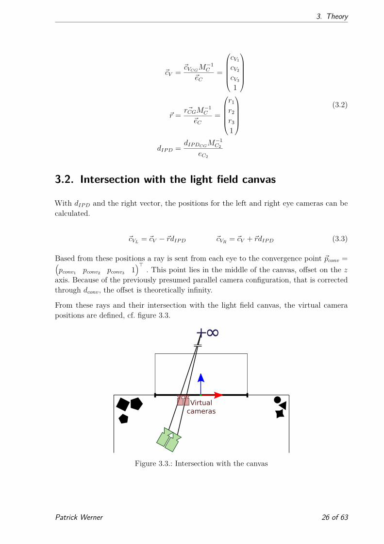
3.2. Intersection with the light field canvas

With dIP D and the right vector, the positions for the left and right eye cameras can be

calculated.

~cVL= ~cV − ~rdIP D ~cVR

= ~cV + ~rdIP D (3.3)

Based from these positions a ray is sent from each eye to the convergence point ~pconv =(

pconv1pconv2

pconv31

)⊤

. This point lies in the middle of the canvas, offset on the z

axis. Because of the previously presumed parallel camera configuration, that is corrected

through dconv, the offset is theoretically infinity.

From these rays and their intersection with the light field canvas, the virtual camera

positions are defined, cf. figure 3.3.

Virtual

cameras

∞

Figure 3.3.: Intersection with the canvas


3. Theory

The straight line going through ~pconv and ~cVLis described by the equation

~l = ~cVL+ tL(~pconv − ~cVL

) (3.4)

and to find the intersection, this must be inserted into the plane normal equation

(~l − ~p0) · ~n (3.5)

with ~p0 = ~0, ~n =(

0 0 1)⊤

and · meaning dot product.

Then, this is solved for

tL =−cVL3

~pconv − cVL3

(3.6)

which is then inserted in ~l. Thus, the intersection point

~cLFL= ~l = ~cVL

+−cVL3

~pconv − cVL3

(~pconv − ~cVL) (3.7)

is calculated. The same steps apply to ~cLFR.

As the rendering requires these coordinates to be in an array coordinate system, the [0, 1]

range is converted to a [0, AmountCameras] range in the x and y axis. This can be ignored

here, as it is a simple scaling.

~cAL=

cLFL1

cLFL2

cLFL3

~cAR=

cLFR1

cLFR2

cLFR3

(3.8)

Now the result of equation 3.1 must be converted to homogeneous 3D coordinates in order

to combine it with the other 3D positions.

~PLFL=

pLFL1

pLFL2

0

1

~PLFR=

pLFR1

pLFR2

0

1

(3.9)


3. Theory

3.3. Calculation of the perceived position

The desired result is the light field position being perceived at a specific position. The

perceived position is formed by the shift from the left to the right eye.

This is achieved by equating the lines starting from the left, and respectively right eye, to

the world point of the object.

~cVL+ k( ~PLFL

− ~cVL) = ~cVR

+ j( ~PLFR− ~cVR

) (3.10)

With the desired position P0 =(

X0 Y0 Z0

)⊤

This can then be solved for dw, as well as

dconv. These formulas 3.11 and 3.12 can then be used to render light field objects at the

desired position P0 when inserted into 3.1.

dw =

−Z0dcVL1

− dcVL1cVL3

+ X0cVL3+ Z0uL − Z0cVL1

− ulcVL3

Z0 − cVL3

−Z0dcVL2

− dcVL2cVL3

+ Y0cVL3+ Z0vL − Z0cVL2

− vlcVL3

Z0 − cVL3

(3.11)

dconv =

diρ1(Z0d − dcVL3− Z0)

Z0 − cVL3

diρ2(Z0d − dcVL3− Z0)

Z0 − cVL3

(3.12)


4. Implementation in the Unreal Engine


As the implementation of a full CG 3D environment would go beyond the scope of this

thesis, an existing environment was chosen. In order to enable the shader based DIBR to

be implemented, the 3D environment had to provide access to the programmable graphics

pipeline, as well as an implementation of a VR API. Additionally, a media functionality

with video support must be available, in order to support video light fields.

These prerequisites were met by the engine Unity as well as the Unreal Engine 4. Subse-

quently the Unreal Engine was chosen as the preferred development environment.

First, the engine itself and its basics are explained. Next, the architecture, as well as the

implementation itself and its multiple classes are demonstrated, followed by the integration

of video data. At last, the additional preparations for the CES are briefly presented.

4.1. General information about the Unreal Engine

The Unreal Engine is a full featured game development tool by Epic Games. It allows

game development in a 2D, 3D or VR environment. Furthermore, it deploys to mobile,

web, console or PC platforms. Most of the following information is taken from the Unreal

Engine website [10], as well as the documentation [11].

It was first publicly released in 1998 along with the game Unreal, supporting development

for high end PCs. The following versions introduced multi platform support while remaining

mainly focused on the high end spectrum. 2014 the current version 4 was released and

over time updated to 4.14.3 as of now.

For beginners it features multiple example projects and free to use assets, which can be

expanded with offers from a marketplace. The engine itself is free to use up to 3000$ of

revenue, afterwards 5% royalties of earnings are required.

Epic Games provides debugging symbols for C++ development and additionally the full

engine source code, that can be extended as desired. Also, support is provided through

forums, AnswerHub, a question answer portal, and an extensive documentation.

An Unreal Engine project has its own folder structure with all content, configurations,

plugins and sources needed. These projects are developed inside the Unreal Editor and

can then be packaged into stand-alone games.

Developers are aided by the UnrealBuildTool, which provides support for various macros

replacing boilerplate code. Additionally, all engine objects are subjected to a garbage

collection.

The development for this thesis started in version 4.13.



4.1.1. Actor

An Actor is the most basic element that can be placed or spawned in a level. It can be

extended with custom functionality and components. These can each feature different

functionality, e.g. light, physics, movement or audio.

During its life cycle it provides different functions accessible via Blueprints, a node based

visual scripting system, or C++ code. For the purposes of this thesis the most important

ones are:

• BeginPlay()

This is executed when the game begins to play, but after the actor is spawned.

• Tick()

This function is executed every frame for every actor.

• BeginDestroy()

This is called when the garbage collection is executed for this actor.

4.1.2. Graphics Programming

The Unreal Engine features the rendering hardware interface (RHI), an abstraction layer

between the graphics API of the system and the engine. Together with a cross compiler

for HLSL1 to other languages, it enables mostly low effort multi platform development.

The architecture of the RHI is mainly based on the DirectX syntax.

There are different feature levels which correspond to different DirectX 11 Shader Models

or OpenGL versions.

In order to keep logic and drawing isolated, the main game thread is separate from the

render thread. The render thread can be accessed by the game thread by enqueuing

rendering commands through macros.

4.1.3. Plugins

The Unreal Engine is highly extensible through plugins, either adding or modifying engine

functionality. These plugins are separate from the engine code and as such separately

compiled. They can consist of multiple modules, e.g. game specific or editor specific

functionality.

Plugins can be specific to a project or made accessible engine-wide, depending on the

install directory.

1DirectX shader language



4.1.4. Media Framework

In order to integrate light field video, media support is necessary. This is available in

Unreal Engines Media Framework, which has recently been completely reworked (4.13)

and as such misses extensive documentation. As the code is completely free to view and

commented, development is still possible. Advanced problems that require more insight

may be described on AnswerHub and are often answered by the developer in a few days.

The available codecs are based on the ones installed on the platform, with basic H.264

profiles being supported best.

Additionally a plugin by the Media Framework developer, providing the VLC2 decoder

functionalities to the engine, is available.

4.1.5. Blueprints

Because the Unreal Engine also wants to appeal to non programmers and should be

accessible even by the artistic game development staff, it features a visual scripting

engine called Blueprints. These enclose most of the engine functionalities in a node based

environment, allowing for complete gameplay scripting from the Unreal Editor. It can

define classes and objects for the engine, using object oriented patterns, cf. figure 4.1.

Figure 4.1.: Blueprint of the SetupSplitMaterialInstances function

2open-source media player by the VideoLAN project



4.2. Architecture

ALightfieldActor

Engine

FViewrenderer Shader

Project

Game

Figure 4.2.: Architecture of the implementation

The foundation of the Unreal Engine based shader structure was supplied by the project

UE4ShaderPluginDemo by Fredrik “Temaran” Lindh [23]. It provided the basic knowledge

needed to implement shaders in the Unreal Engine 4.11. In the scope of this thesis it was

ported to version 4.13.

In order to keep everything structured and portable, the engine code should not be modified,

keeping the code on a project basis.

The Fraunhofer IIS DIBR shader code is provided in separate shader files. These shaders

are wrapped by a plugin called FViewrenderer, that implements the complete light field

rendering inside of an independent plugin.

Connection to the game itself is provided by the class ALightfieldActor, the representa-

tion of the canvas object in the game. It collects all needed parameters and passes them

to the FViewrenderer plugin, which returns the finished image (cf. figure 4.2).

For video functionality a workaround, thoroughly discussed in 4.5, is provided in the

ULightfieldMediaTexture class.

In addition to the general classes, there is also a LightfieldEditor subdirectory where

Editor specific classes are defined, such as the ULightfieldMediaTextureFactory which

provides access to the ULightfieldMediaTexture in the Editor user interface.

All of the used Blueprint functions, as well as the publicly available members of the most

important classes can be found in the appendices A and B.

4.3. FViewrenderer plugin

The FViewrenderer plugin wraps the Fraunhofer IIS DIBR shaders. Its aim is to decouple

the rendering process from the game logic, by exposing a public API. Through this the

rendering can be started and the results accessed. As the DIBR shaders provide optional

filtering, an enum of filtering types is supplied.

In theory the constructor accepts all invariant parameters for a light field data set, while

the public ExecuteComputeShader() method accepts the varying parameters.



However, some of the typically constant parameters are supplied in the execution method for

the sake of dynamically changing and testing parametrization. Furthermore, the resulting

rendered RGBA3 images or disparity maps can be accessed through the corresponding

getter methods.

In the constructor all of the needed textures are created. As described in chapter 3, the

most important parameters of ExecuteComputeShader() are the eye positions ~cLFL, ~cLFR

and the desired position P0. Other parameters include the needed textures, as well as

various parameters for the calculation of the virtual camera position and the nearest

cameras. At first, the method checks if any textures have changed and recreates them if

needed. Next the virtual camera positions are calculated from the passed positions and the

array setup defined in the constructor. Now the specified amount of neighbouring cameras

to these positions are calculated through sorting the distances to them.

The next step is the calculation of dw and dconv as described in equations 3.12 and 3.11.

Up until now everything was executed on the game thread. For the sake of executing

rendering code, a transition to the render thread must be performed. The private function

ExecuteComputeShaderInternal() is now enqueued onto the render threads task list

with a macro.

In this method the individual shader implementations are invoked in the order explained

in 2.1.3.

As the FViewrenderer plugin uses compute shaders, the latest feature level SM5 has to

be supported by the hardware, which roughly corresponds to D3D11 Shader Model 5 or

OpenGL 4.3.

4.3.1. Compute shader implementation: FForwardWarpDeclaration

Because the implementations of the compute shaders are very similar, it will be explained

on the example of the forward warp shader.

The shaders provided by Fraunhofer IIS have different input and output surfaces, as

well as parameters according to the step represented. The class itself has to extend the

FGlobalShader class, which supplies a constructor parameter that can be used to bind

these surfaces to the shader. On the other hand the parameters are supplied through a

uniform buffer struct.

Checks for outdated surfaces are possible through the Serialize() function. To set these

input and output surfaces to their respective textures the method SetSurfaces() is

provided.

Similarly, methods that bind and unbind the parameter uniform buffer structs are imple-

mented.

3additional alpha channel which describes translucency



In order to be accepted by the engine as a shader, it also needs to supply functions pointing

to the specific shader files, as well as their main function’s name.

These steps are nearly analogous for the other compute shader types.

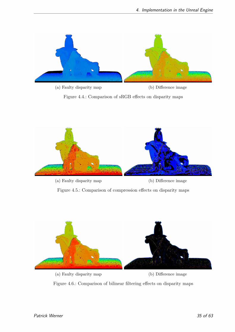
4.3.2. Quality improvements

At first the disparity maps loaded into the engine were deviating from the source material,

which lead to artefacts in the end results.

This was caused by multiple factors. As the source disparity maps are raw data, no sRGB4

conversion should be applied to them, due to heavy alteration of the disparity values.

Another quality deficiency was caused by the texture filtering method of the GPU, set

to bi-linear by default. Because this creates non-existent disparities by interpolation, it

should be fixed. The last flaw was caused by the lossy compression applied to the texture,

which created a streaking effect in the disparity maps.

These settings can be set for each texture individually in the Texture Editor. Here sRGB

can be disabled, the filtering can be set to Nearest and finally the compression can

be set to an uncompressed, and as such not affecting the texture quality, format like

VectorDisplacementMap.

Figure 4.3.: Correct disparity map

The effects of these settings were tested on the Cleopatra data set after the forward warping

step. As can be seen in figures 4.4, 4.5 and 4.6 the sRGB conversion has the biggest impact

on the quality, followed by the compression and at last the filtering. Interestingly the

compression artefacts can be clearly distinguished.

Furthermore, a mean squared error (MSE) comparison verified these results, cf. table

4.1.

Method sRGB compression filtering

MSE 12520 562 149

Table 4.1.: MSEs for texture settings

4colour space with increased luminance, used for accurate representation on computer monitors



(a) Faulty disparity map (b) Difference image

Figure 4.4.: Comparison of sRGB effects on disparity maps


Figure 4.5.: Comparison of compression effects on disparity maps


Figure 4.6.: Comparison of bilinear filtering effects on disparity maps



4.4. ALightfieldActor

The ALightfieldActor defines the physical representation of a light field inside the game

engine. Its foundations are laid in a C++ class and extended via a Blueprint. In general

it connects the canvas object and its intrinsic parameters to the FViewrenderer plugin

and displays its results on the canvas. All needed parameters are either specifiable in the

Unreal Editor for each ALightfieldActor or derivable from the environment.

The canvas model was created in Blender5 and features special canvas texture coordinates,

which map the texture fully on the front and back sides.

4.4.1. C++

ALightfieldActor is derived from AStaticMeshActor, a base class for actors that always

have a mesh attached. In this case it is the aforementioned canvas mesh.

Every class that should be available in game needs the UCLASS() macro before the class

declaration, which helps generate Unreal’s own representation of a class. Here the specifier

Blueprintable is passed, as this allows the class to be extended by a Blueprint.

Similarly all the methods or member variables have macros defining the visibility and

accessibility in the Unreal Editor environment. C++ specific members can be declared

without macros.

Most of the variables are initialized in the constructor. However, some of them depend on

the game running, these are initialized later in the BeginPlay() method.

As the viewrenderer depends on the resolution of the textures to be initialized, which

are not always available after BeginPlay() has executed, it is initialized with the

InitViewrenderer() function. This function may also be called from a Blueprint and

as such is marked as BlueprintCallable. Here the FViewrenderer plugin and a pixel

shader plugin [23], used to convert the compute shader output, are instanced and assigned

to pointers.

In the Tick() function the textures that should be passed to the viewrenderer are first filled

depending on the selected SourceType. Then the parameters are converted as described

in chapter 3 and finally passed to the FViewrenderer plugin.

At last, the pointers to the plugin instances need to be freed. The BeginDestroy() method

does this at the end of the actors life cycle.

5a open-source 3D computer graphics software



4.4.2. Blueprint

The Blueprint class extends most of the functionalities based in the C++ code. In the

Blueprint most of the initialization of the textures is done. Depending on the source type,

either the video or the still images are loaded.

Then the resulting render targets are created and assigned to the variables created in

C++.

In the end an instance of the light field material is created, which uses the render targets

assigned before.

4.4.3. LightfieldMaterial

Materials are applied to meshes and handle their appearance in the engine. They provide

a variety of input data, which can be used to create physically based shading. Additionally,

different shading models, like Default Lit, Unlit or Subsurface, can be determined. Similar

to other features in the engine, a custom editor interface is provided to create these

materials in a node based fashion.

The LightfieldMaterial is in charge of displaying the correct texture on the light field

actor. It uses the texture coordinates supplied by the canvas mesh to map the result of

the viewrendering to the mesh.

It also enables the stereo support for VR by displaying different textures for each eye.

This is possible through the ScreenPosition coordinates, these span the screen in x and

y direction in a range from 0.0 to 1.0. By applying one texture from 0.0 to 0.5 and one

from 0.5 to 1.0 horizontally, the eyes can be separated.

In addition it handles the alpha support for the light field depending on the alpha channels

supplied by the FViewrenderer plugin.

4.5. Embedding of video data

The next step is to provide the viewrenderer with video data instead of static images. At

first, the video data has to be created in a sensible way. Due to the synchrony problems

and high inefficiency of accessing multiple video files at once, a different approach needed

to be made. Because the Unreal Engine does not supply easy access to multi view data,

that may be supported through a multi view codec, as described in Section 2.4, solutions

using existing functionalities were necessary.

Two approaches meeting these requirements were implemented. On one hand all videos

are combined into one, possibly higher resolution, video with all the needed images and

disparity maps. On the other hand placing the views behind each other on the timeline.



Another novelty is that the media file has to be specifically opened. Because the FViewrenderer

plugin depends on the media’s resolution, this has to happen beforehand. A solution is

provided through a delegate that registers to the OnMediaOpened event, which is called as

soon as the media file has finished opening. Then the viewrenderer can be initialized.

The next data set, called reporter, is a 4 × 4 shot recorded with a camera array composed

of modified GoPro cameras. It then went through the light field processing chain, as well

as a keying process, resulting in a data set with transparencies. The following sections are

explained on the basis of this reporter data set.

For video conversion and coding the FFmpeg software was used. To ensure support by the

Windows 7 codecs, while maintaining portability, the H.264 codec was used with the high

profile and level 4.0.

With this codec Windows 7 only supports resolutions up to FHD, while the Windows

specific WMV6 format supports up to UHD. However, a bug in version 4.14, which makes

textures appear too bright, renders this format unusable for now.

4.5.1. High resolution

The first approach works through combining all needed images and disparity maps into

one video. Because the incoming images are now made up of multiple views as shown in

figure 4.7 they have to be split up again.

Figure 4.7.: Incoming video data (increased gamma)

This is solved via an Unreal Engine specific solution. By creating a splitting material, that

only renders tiles of the input texture onto a render target. This material has multiple

parameters through which it only renders parts of the input texture.

6Windows Media Video



The necessary initializations are provided in Blueprints, starting at the SetupForHighResVideo

function. Here the different material instances needed for every view are instanced, then

for each instance a render target is created.

In the SetupSplitmaterialInstances function the number of cameras, currently only

horizontal, is used to create and parametrize the SplitMaterial instances. In the end

these are added to an array which was previously declared in C++.

Next, for each material instance a render target is created with the special settings

described in section 4.3.2. Similar to the instances, these are also saved in an array.

In the C++ Tick() function these arrays are then used to draw to the render targets

with the DrawMaterialToRendertarget() function.

A problem arose where the last texture passed to the viewrenderer was black. Assuming

this is a result of the draw process not being fast enough before assigning the targets, GPU

synchronisation is required. This is done with the FlushRenderingCommands() function.

However the last texture was still black. Now a workaround is implemented, which draws

a material to a dummy texture after the last render target.

The targets are then used as the textures passed to the viewrenderer.

Limitations

This approach currently has some limitations. The first one is the overhead of the Unreal

Engine specific SplitMaterial method. Instead, the textures may be split using RHI

functions.

Another limitation is the supported resolution. FFmpeg uses 4:4:4 predictive behaviour

when coding resolutions higher than FHD. This is not supported by the standard Windows

7 H.264 decoder implementation. Because of this the resolution is limited to FHD, that

limits the amount of camera views that can be used, while keeping the quality acceptable.

A possible fix is provided by the previously mentioned VLC plugin, with this the resolution

can be raised to UHD, resulting in higher individual resolutions.

In general both methods have a common limitation, the data loss when the disparity

is encoded. Because the original data is made up of floating point values, the resulting

disparities cannot be fully correct. This is further explored in section 5.2.

4.5.2. High frame rate

Instead of arranging the images next to each other, the other approach is to put them

behind each other. Then the resulting video is read with a higher frame rate than the

original data, depending on the amount of views used.

The decoding of the media happens on its own thread, which supplies the textures according

to the media frame rate. Because of this the individual textures cannot easily be accessed



in the game thread Tick() method. A solution was to extend the existing UMediaTexture

with a specialized ULightfieldMediaTexture.

Instead of providing one public resource, it provides an array of the last few decoded

textures. These can then be accessed by the game thread to pass the textures to the

viewrenderer.

Because a UMediaTexture can be created in the Editor environment, and the function-

ality should be equivalent in the ULightfieldMediaTexture a factory class has to be

created. This factory class is only available in the editor and provides access to the

ULightfieldMediaTexture as an asset.

Limitations

The main limitation is the decoding speed. This (central processing unit (CPU) or GPU)

bottleneck limits the amount of concurrently usable views. Another one is the relatively

high amount of “workaround” code, which compromises maintainability. Occasionally the

high frame rate video is offset by one frame, leading to errors in the viewrendering.

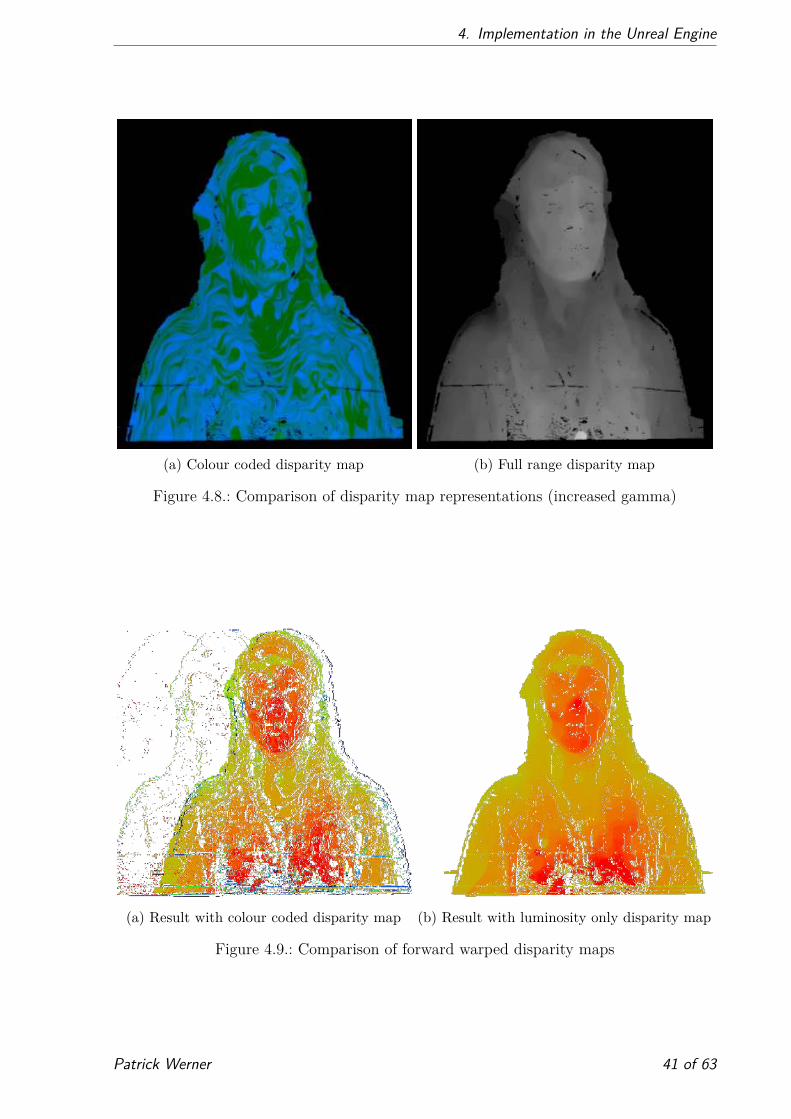
4.5.3. Quality improvements

At first, the standard colour coded variants of the disparity maps, described in section

2.1.2, were used. The resulting renderings had significant artefacts.

As the H.264 codec converts the RGB values to the YCbCr colour model, assuming the

video consists of standard, not data, content. When this is decoded, non existing colour

values can be found in other channels.

Instead of colour coding the disparity maps, they are spread to fully span the available 8

bit colour range in all three channels, as shown in figure 4.8. The used values are then

passed to the shader, where the disparities are converted back to their true values. The

results are significantly better, as can be seen in the forward warped disparity maps in

figure 4.9.

4.6. Preparation for CES

In order to have a more interactive CES demonstrator some smaller Blueprint classes were

created. Interactable objects such as buttons, switches or blocks, which activate objects

implementing the Activatable interface such as lights or moving blocks. Interaction is

provided mostly via the MotionControllerPawn from the VR example map. Additionally,

a torch was added to one of the VR controllers drastically increasing the immersion with

the Cleopatra scene.



(a) Colour coded disparity map (b) Full range disparity map

Figure 4.8.: Comparison of disparity map representations (increased gamma)

(a) Result with colour coded disparity map (b) Result with luminosity only disparity map

Figure 4.9.: Comparison of forward warped disparity maps



Also, an Egyptian tomb themed scene was created (cf. figure 4.11) in order to highlight

the captured scenes. In addition to the Cleopatra data set, a complete room filled with

Egyptian artefacts, called the burial chamber data set, was created, cf. figure 4.10. This

new data set highlighted the need for a positional correction even more, as the walls needed

to line up with the CG walls to create an immersive experience.

Figure 4.10.: Burial chamber data set

Figure 4.11.: Egyptian tomb setting with torch (increased gamma)


5. Evaluation

5. Evaluation

The aim of this chapter is to evaluate the success of the theory explained in chapter 3 in

integrating the light field objects inside the CG environment. At first a 3D cube is placed

at specific points in front or behind the light field canvas, then the behaviour of the light

field in comparison to the object is examined. Then the impact of compression on the

resulting disparity maps is evaluated, followed by the performance. At last subjective user

feedback is inspected.

5.1. Comparison with a 3D object

In order to test the light field rendering, a cube is placed in different points in front, behind

and inside the 3D canvas. The cube is applied with a material that is always visible to the

camera. Then the camera is moved in different directions and the relative movement of

the light field is compared to the cube. Everything works as intended when the light field

behaves in the same way as the cube. For this a 5 × 3 segment of the Cleopatra data set is

used.

The cube is placed on Cleopatra’s right eye in the same plane as the canvas. At first no

additional parameters are passed to the FViewrenderer plugin, here the object behaves

like it is in front of the cube, cf. figure 5.1.

The parameters can now be modified, so the cube matches the eye, cf. figure 5.2.


5. Evaluation

Figure 5.1.: Camera movement from top left to bottom right without modification (increasedgamma)


5. Evaluation

Figure 5.2.: Camera movement from top left to bottom right with modification (increasedgamma)


5. Evaluation

5.2. Impact of video compression

Because of the better stability the high frame rate variant was chosen for this section.

In order to evaluate the effects of video compression on the disparity maps accurately, a

single uncompressed file went through FFmpeg downscaling to 480 × 540 and the Unreal

Engine upscaling back to 900 × 900. The videos were encoded with the high 4.0 profile

using the Lavc encoder and yuv420p pixel format. The variable value is the constant rate

factor (CRF) which defines the quality level descending from 0 to 51. As a comparison

metric the MSE is used. The compression does not have as big of an impact with lower

CRF values, however values higher than 20 should have a significant visual impact, as can

be observed from the values listed in table 5.1.

CRF 1 10 20 30 40

Bitrate in kB/s 39717 15262 4847 1066 218MSE 0.56 1.53 2.80 12.58 43.02

Table 5.1.: Comparison of compression impact on disparity maps

5.3. Performance

The demonstrator was mostly developed on the same PC. It features a NVIDIA GeForce

1060 GPU with 6GB of memory, which is the most important aspect for the performance.

Its CPU is a Intel Core i7-6700 with 3.40 GHz. The VR aspect was covered by a HTC

Vive.

Performance was tested on the Cleopatra data set, the burial chamber data set and the

reporter data set. Furthermore, two dynamic light sources had a high impact on the

performance, but immensely improved the immersion. For the video the high resolution

variant has been chosen, with a frame rate of 25 frames per second and FHD resolution.

The goal was to achieve a stable frame rate of 90 frames per second, with the available

settings. Results are listed in table 5.2.

Dataset Cleopatra Cleopatra burial chamber reporter

Resolution 1920 × 1080 1100 × 618 750 × 422 480 × 540Amount of views used 1 5 12 4Filtering method none median none median

Table 5.2.: Settings for stable frame rate with two dynamic light sources

As can be observed, a compromise between resolution and amount of views used has to be

made. Higher resolutions produce crisper images, however with more views the resulting

rendering has less occlusions. As a consequence, the specific settings should depend on the

input data and its requirements.


5. Evaluation

5.4. User feedback

During the course of this thesis the demo was tested by a multitude of people. Without the

modifications described in chapter 3 users reported that the Cleopatra object felt out of

place and moved in strange ways. Especially the burial chamber produced peculiar effects,

due to the added walls that did not line up with the CG walls.

The modification vastly improved the integration, users reported Cleopatra definitely felt

like it was there in the CG world. This was amplified by the addition of the torch, which

enabled casting shadows of Cleopatra. Similarly, the burial chamber felt a lot more natural

and integrated into the scene.

However, the stereoscopic effect is static when moving towards or away from the canvas,

leading to a flatter impression as the viewer is closer and respectively deeper when the

viewer is further away. This may be a result of the missing third dimension in the light

field rendering.


6. Conclusion

6. Conclusion

In this thesis the creation of a demonstrator, which enables the integration of light field

data in the 3D environment of the Unreal Engine 4 was described.

First, the foundations needed were examined, consisting of light field, 3D and digital video

basics. Then, these were used to devise a projection model for the seamless integration of

light field data. With this model a position for the captured object in relation to the light

field canvas can be chosen.

This was followed by the explanation of the Unreal Engine and the implementation of

the demonstrator itself. Using the available tools of the engine and the Fraunhofer DIBR

shaders the demonstrator was realised. By applying the projection model the seamless

connection of the coordinate systems was ensured. Especially the integration of light field

video data was explored, by devising two distinct methods. Together with new content

this resulted in an immersive demonstrator, presented at the CES.

At last, the demonstrator was evaluated piece by piece. The projection model’s functionality

was shown at the hand of a 3D object, as well as with user feedback. Furthermore, the effects

of video compression on the video light field data and the demonstrators performance,

explore the demonstrators boundaries.

6.1. Outlook

The demonstrator devised in this thesis has a lot of room to grow. While many small

improvements can be made to the code base, the main factors lie in the algorithms. As

the formulas derived in chapter 3 are not definitive, their enhancement may produce an

even more immersive experience. Additionally, the light field rendering may be extended

to feature full 3D rendering.

The input quality and efficiency of video data may be increased with the new H.265 codec

and multi view coding, leading to more available data to the renderer. This may raise

rendering quality and freedom of movement. Because of the relative independence from the

shaders, the demonstrator may be used to depict different light field rendering techniques.

Different array layouts may also improve the usage scenarios, by enabling e.g full 360°

walk arounds of dynamic light field objects.

Interactive light fields, e.g. a real barkeeper reacting to prompts, may enrich gaming or

VR applications. A different approach might be an artificial relighting in the light field.

By using the torch to correctly relight objects inside the light field, immersion can be

improved immensely.

As can be seen future possibilities are plenty, especially with ever evolving light field and

VR technologies.


Bibliography

Bibliography

[1] Edward H Adelson and James R Bergen. The plenoptic function and the elements of

early vision. 1991.

[2] Ronald T Azuma. A survey of augmented reality. Presence: Teleoperators and virtual

environments, 6(4):355–385, 1997.

[3] Marcelo Bertalmio, Guillermo Sapiro, Vincent Caselles, and Coloma Ballester. Image

inpainting. In Proceedings of the 27th annual conference on Computer graphics and

interactive techniques, pages 417–424. ACM Press/Addison-Wesley Publishing Co.,

2000.

[4] Steven Boyer. A virtual failure: Evaluating the success of Nintendo’s Virtual Boy.

The Velvet Light Trap, (64):23–33, 2009.

[5] Jie Chen, Junhui Hou, and Lap-Pui Chau. Light field compression with disparity

guided sparse coding based on structural key views. arXiv preprint arXiv:1610.03684,

2016.

[6] Łukasz Dąbała, Matthias Ziegler, Piotr Didyk, Frederik Zilly, Joachim Keinert, Karol

Myszkowski, H-P Seidel, Przemysław Rokita, and Tobias Ritschel. Efficient multi-

image correspondences for on-line light field video processing. In Computer Graphics

Forum, volume 35, pages 401–410. Wiley Online Library, 2016.

[7] Christoph Fehn. A 3D-TV approach using depth-image-based rendering (DIBR). In

Proc. of VIIP, volume 3, 2003.

[8] Christoph Fehn. Depth-image-based rendering (DIBR), compression, and transmission

for a new approach on 3D-TV. In Electronic Imaging 2004, pages 93–104. International

Society for Optics and Photonics, 2004.

[9] Siegfried Foessel, Frederik Zilly, Michael Schöberl, Peter Schäfer, Matthias Ziegler, and

Joachim Keinert. Light-field acquisition and processing system for film productions.

In Annual Technical Conference & Exhibition, SMPTE 2013, pages 1–8. SMPTE,

2013.

[10] Epic Games. Unreal Engine. https://www.unrealengine.com/

what-is-unreal-engine-4/. [Online; accessed 20.01.2017].

[11] Epic Games. Unreal Engine Documentation. https://docs.unrealengine.com/.

[Online; accessed 20.01.2017].

[12] M Heilig. Sensorama simulator. United States Patent and Trade Office, Virginia,

USA, US-3,050,870, 1962.

[13] Google Inc. Google Jump. https://vr.google.com/jump/. [Online; accessed

20.01.2017].


https://www.unrealengine.com/what-is-unreal-engine-4/

https://www.unrealengine.com/what-is-unreal-engine-4/

https://docs.unrealengine.com/

https://vr.google.com/jump/

Bibliography

[14] Khronos Group Inc. OpenGL Rendering Pipeline. https://www.khronos.org/

opengl/wiki/Rendering_Pipeline_Overview. [Online; accessed 20.01.2017].

[15] Lytro Inc. Lytro Cinema. https://www.lytro.com/cinema/. [Online; accessed

20.01.2017].

[16] Lytro Inc. Lytro Illum. https://www.lytro.com/illum/. [Online; accessed

11.01.2017].

[17] Lytro Inc. Lytro Immerge. https://www.lytro.com/immerge/. [Online; accessed

20.01.2017].

[18] Shahram Izadi, David Kim, Otmar Hilliges, David Molyneaux, Richard Newcombe,

Pushmeet Kohli, Jamie Shotton, Steve Hodges, Dustin Freeman, Andrew Davison,

et al. Kinectfusion: real-time 3D reconstruction and interaction using a moving depth

camera. In Proceedings of the 24th annual ACM symposium on User interface software

and technology, pages 559–568. ACM, 2011.

[19] Peter Kauff, Nicole Atzpadin, Christoph Fehn, Marcus Müller, Oliver Schreer, Aljoscha

Smolic, and Ralf Tanger. Depth map creation and image-based rendering for advanced

3DTV services providing interoperability and scalability. Signal Processing: Image

Communication, 22(2):217–234, 2007.

[20] Péter Tamás Kovács, Zsolt Nagy, Attila Barsi, Vamsi Kiran Adhikarla, and Robert

Bregovic. Overview of the applicability of H.264/MVC for real-time light-field

applications. In 3DTV-Conference: The True Vision-Capture, Transmission and

Display of 3D Video (3DTV-CON), 2014, pages 1–4. IEEE, 2014.

[21] Marc Levoy. Light fields and computational imaging. Computer, 39(8):46–55, 2006.

[22] Marc Levoy and Pat Hanrahan. Light field rendering. In Proceedings of the 23rd

annual conference on Computer graphics and interactive techniques, pages 31–42.

ACM, 1996.

[23] Fredrik Lindh. UE4ShaderPluginDemo. https://github.com/Temaran/

UE4ShaderPluginDemo/. [Online; accessed 11.01.2017].

[24] Karsten Müller, Heiko Schwarz, Detlev Marpe, Christian Bartnik, Sebastian Bosse,

Heribert Brust, Tobias Hinz, Haricharan Lakshman, Philipp Merkle, Franz Hunn

Rhee, et al. 3D high-efficiency video coding for multi-view video and depth data.

IEEE Transactions on Image Processing, 22(9):3366–3378, 2013.

[25] Ren Ng, Marc Levoy, Mathieu Brédif, Gene Duval, Mark Horowitz, and Pat Hanrahan.

Light field photography with a hand-held plenoptic camera. Computer Science

Technical Report CSTR, 2(11):1–11, 2005.

[26] Christian Riechert, Frederik Zilly, Marcus Müller, and Peter Kauff. Advanced inter-

polation filters for depth image based rendering. In 3DTV-Conference: The True

Vision-Capture, Transmission and Display of 3D Video (3DTV-CON), 2012, pages

1–4. IEEE, 2012.


https://www.khronos.org/opengl/wiki/Rendering_Pipeline_Overview

https://www.khronos.org/opengl/wiki/Rendering_Pipeline_Overview

https://www.lytro.com/cinema/

https://www.lytro.com/illum/

https://www.lytro.com/immerge/

https://github.com/Temaran/UE4ShaderPluginDemo/

https://github.com/Temaran/UE4ShaderPluginDemo/

Bibliography

[27] Daniel Scharstein and Richard Szeliski. A taxonomy and evaluation of dense two-

frame stereo correspondence algorithms. International journal of computer vision,

47(1-3):7–42, 2002.

[28] Daniel Scharstein, Richard Szeliski, and Heiko Hirschmüller. Middlebury Stereo

Evaluation. http://vision.middlebury.edu/stereo/eval3/. [Online, accessed

20.01.2017].

[29] Peter Shirley, Michael Ashikhmin, and Steve Marschner. Fundamentals of Computer

Graphics. CRC Press, 2009.

[30] Ivan E Sutherland. A head-mounted three dimensional display. In Proceedings of the

December 9-11, 1968, fall joint computer conference, part I, pages 757–764. ACM,

1968.

[31] Bennett Wilburn, Neel Joshi, Vaibhav Vaish, Eino-Ville Talvala, Emilio Antunez,

Adam Barth, Andrew Adams, Mark Horowitz, and Marc Levoy. High performance

imaging using large camera arrays. In ACM Transactions on Graphics (TOG),

volume 24, pages 765–776. ACM, 2005.

[32] Frederik Zilly, Michael Schöberl, Peter Schäfer, Matthias Ziegler, Joachim Keinert, and

Siegfried Foessel. Lightfield media production system using sparse angular sampling.

In ACM SIGGRAPH 2013 Posters, page 102. ACM, 2013.

[33] Frederik Zilly, Matthias Ziegler, Joachim Keinert, Michael Schoberl, and Siegfried

Foessel. Computational imaging for stop-motion animated video productions. SMPTE

Motion Imaging Journal, 125(1):42–47, 2016.

[34] C Lawrence Zitnick, Sing Bing Kang, Matthew Uyttendaele, Simon Winder, and

Richard Szeliski. High-quality video view interpolation using a layered representation.

In ACM Transactions on Graphics (TOG), volume 23, pages 600–608. ACM, 2004.


http://vision.middlebury.edu/stereo/eval3/

A. Blueprints

A. Blueprints

Fig

ure

A.1

.:N

ode

layo

ut

ofth

eLightfieldMaterial


A. Blueprints

Fig

ure

A.2

.:C

ut

out

ofth

eALightfieldActor

blu

epri

nt

Beg

inP

lay

node

tree

Fig

ure

A.3

.:B

luep

rint

ofth

eSetupForHighResVideo

funct

ion


A. Blueprints

Fig

ure

A.4

.:B

luep

rint

ofth

eSetupLightfieldMaterial

funct

ion

Fig

ure

A.5

.:B

luep

rint

ofth

eSetResultRenderTarget

funct

ion


A. Blueprints

Fig

ure

A.6

.:T

he

SplitMaterial

setu

p


A. Blueprints

Fig

ure

A.7

.:B

luep

rint

ofth

eOpenMediaSource

funct

ion

Fig

ure

A.8

.:B

luep

rint

ofth

eSetupSplitRenderTargets

funct

ion


A. Blueprints

Fig

ure

A.9

.:L

oop

body

ofth

eSetupSplitMaterialInstances

funct

ion


B. Code Listings of public members


Listing B.1: Public methods of the ALightfieldActor class1 // Sets default values for this actor ’s properties

ALightfieldActor ();

3

// Called when the game starts or when spawned

5 virtual void BeginPlay () override ;

virtual void BeginDestroy () override ;

7

// Called every frame

9 virtual void Tick( float DeltaSeconds ) override ;

11 UFUNCTION ( BlueprintCallable , Category = " Lightfield ", meta = ( BlueprintProtected ))

void InitViewrenderer ();

Listing B.2: Public members of the ULightfieldMediaTexture classbool CheckIfLoadedAndInit ( const uint32 NumTex );

2

TArray < class FTextureResource *> Resources ;

4

virtual void UpdateTextureSinkBuffer ( const uint8 * Data , uint32 Pitch = 0) override ;

6 virtual void ShutdownTextureSink () override ;

Listing B.3: Public methods of the FViewrenderer pluginFViewrenderer ( const uint8 NX , const uint8 NY , const float N,

2 const int32 SizeX , const int32 SizeY ,

const bool bIsLinearColor , const bool bIsStereo , const bool bIsVideoData ,

4 const ERHIFeatureLevel :: Type ShaderFeatureLevel );

6 ~ FViewrenderer ();

8 void ExecuteComputeShader ( const TArray < FTexture2DRHIRef >& InputRgbaTextures ,

const TArray < FTexture2DRHIRef >& InputDispTextures ,

10 const uint8 Amount , const float Multiplier ,

const EFilterType FilterType , const bool bInpaint ,

12 const FVector & CameraPositionLeft ,

const FVector & CameraPositionRight ,

14 const FVector2D & DesiredPosition ,

const float DesiredZ_X , const float DesiredZ_Y ,

16 const float DesiredDisparity ,

const FVector & EyeDistance , const float ConvergenceDistance );

18

void ExecuteComputeShaderInternal (); // Only execute from render thread

20

FORCEINLINE FTexture2DRHIRef GetRgbaTexture ( const uint8 Eye) const

22 {

return ResultRgbaTextures [Eye ];

24 }

26 FORCEINLINE FTexture2DRHIRef GetDispTexture ( const uint8 Eye) const

{

28 return ResultDispTextures [Eye ];

}



Listing B.4: Public methods of the FForwardWarpDeclaration compute shader1 FForwardWarpDeclaration () {}

3 explicit FForwardWarpDeclaration ( const ShaderMetaType :: CompiledShaderInitializerType &

Initializer );

5

static bool ShouldCache ( EShaderPlatform Platform )

7 {

return IsFeatureLevelSupported (Platform , ERHIFeatureLevel :: SM5 );

9 }

11 static void ModifyCompilationEnvironment ( EShaderPlatform Platform ,

FShaderCompilerEnvironment & OutEnvironment );

13

virtual bool Serialize ( FArchive & Ar) override

15 {

bool bShaderHasOutdatedParams = FGlobalShader :: Serialize (Ar );

17

Ar << InputDispSurface << OutputDispSurfaceLeft << OutputDispSurfaceRight ;

19

return bShaderHasOutdatedParams ;

21 }

23 // This function is required to let us bind our runtime surface to the shader using an UAV

void SetSurfaces ( FRHICommandList & RHICmdList ,

25 FShaderResourceViewRHIRef InputDispSurfaceSRV ,

FUnorderedAccessViewRHIRef OutputDispSurfaceUAV );

27

void SetSurfacesStereo ( FRHICommandList & RHICmdList ,

29 FShaderResourceViewRHIRef InputDispSurfaceSRV ,

FUnorderedAccessViewRHIRef OutputDispSurfaceUAVLeft ,

31 FUnorderedAccessViewRHIRef OutputDispSurfaceUAVRight );

33 // This function is required to bind our constant / uniform buffers to the shader .

void SetUniformBuffers ( FRHICommandList & RHICmdList ,

35 const FForwardWarpVariableParameters & VariableParameters );

37 // This is used to clean up the buffer binds after each invocation to let them be changed

// and used elsewhere if needed .

39 void UnbindBuffers ( FRHICommandList & RHICmdList );

41 static const TCHAR * GetSourceFilename () {

return TEXT(" ForwardWarp ");

43 }

45 static const TCHAR * GetFunctionName () {

return TEXT(" ForwardWarpComputeShader ");

47 }


C. List of Figures

C. List of Figures

1.1. Overview of this thesis . . . . . . . . . . . . . . . . . . . . . . . . . . . . . 8

2.1. An eye gathering light rays . . . . . . . . . . . . . . . . . . . . . . . . . . . 92.2. Line gantry at Fraunhofer IIS . . . . . . . . . . . . . . . . . . . . . . . . . 102.3. The Lytro Illum plenoptic camera [16] . . . . . . . . . . . . . . . . . . . . 102.4. Black magic 3 × 3 camera array . . . . . . . . . . . . . . . . . . . . . . . . 112.5. The Fraunhofer IIS light field rendering workflow . . . . . . . . . . . . . . 122.6. The Cleopatra object captured . . . . . . . . . . . . . . . . . . . . . . . . . 122.7. Rectified images of the Cleopatra figurine. The rectangle shows the aligned

pixels. . . . . . . . . . . . . . . . . . . . . . . . . . . . . . . . . . . . . . . 132.8. Disparity estimation of the cat ear. The ear can be found in the adjacent

image shifted by the disparity. . . . . . . . . . . . . . . . . . . . . . . . . 142.9. Comparison of disparity post-processing outcome . . . . . . . . . . . . . . 142.10. Viewrendering in a 2 × 2 array . . . . . . . . . . . . . . . . . . . . . . . . . 152.11. Forward warping . . . . . . . . . . . . . . . . . . . . . . . . . . . . . . . . 162.12. Backward warping . . . . . . . . . . . . . . . . . . . . . . . . . . . . . . . 162.13. Merged colour image . . . . . . . . . . . . . . . . . . . . . . . . . . . . . . 172.14. Dice before (left) and after (right) the rotation around the y axis . . . . . . 182.15. Camera with up(y), forward(-z) and right(x) vector . . . . . . . . . . . . . 192.16. View transformation . . . . . . . . . . . . . . . . . . . . . . . . . . . . . . 202.17. OpenGL rendering pipeline [14] . . . . . . . . . . . . . . . . . . . . . . . . 212.18. Comparison between pinhole camera and rasterization rendering . . . . . . 22

3.1. Resulting object movement when rendering virtual camera views (V) be-tween real cameras (R) . . . . . . . . . . . . . . . . . . . . . . . . . . . . . 24

3.2. Top down view of the 3D scene . . . . . . . . . . . . . . . . . . . . . . . . 253.3. Intersection with the canvas . . . . . . . . . . . . . . . . . . . . . . . . . . 26

4.1. Blueprint of the SetupSplitMaterialInstances function . . . . . . . . . 314.2. Architecture of the implementation . . . . . . . . . . . . . . . . . . . . . . 324.3. Correct disparity map . . . . . . . . . . . . . . . . . . . . . . . . . . . . . 344.4. Comparison of sRGB effects on disparity maps . . . . . . . . . . . . . . . . 354.5. Comparison of compression effects on disparity maps . . . . . . . . . . . . 354.6. Comparison of bilinear filtering effects on disparity maps . . . . . . . . . . 354.7. Incoming video data (increased gamma) . . . . . . . . . . . . . . . . . . . 384.8. Comparison of disparity map representations (increased gamma) . . . . . . 414.9. Comparison of forward warped disparity maps . . . . . . . . . . . . . . . . 414.10. Burial chamber data set . . . . . . . . . . . . . . . . . . . . . . . . . . . . 424.11. Egyptian tomb setting with torch (increased gamma) . . . . . . . . . . . . 42

5.1. Camera movement from top left to bottom right without modification(increased gamma) . . . . . . . . . . . . . . . . . . . . . . . . . . . . . . . 44

5.2. Camera movement from top left to bottom right with modification (increasedgamma) . . . . . . . . . . . . . . . . . . . . . . . . . . . . . . . . . . . . . 45


C. List of Figures

A.1. Node layout of the LightfieldMaterial . . . . . . . . . . . . . . . . . . . 52A.2. Cut out of the ALightfieldActor blueprint BeginPlay node tree . . . . . 53A.3. Blueprint of the SetupForHighResVideo function . . . . . . . . . . . . . . 53A.4. Blueprint of the SetupLightfieldMaterial function . . . . . . . . . . . . 54A.5. Blueprint of the SetResultRenderTarget function . . . . . . . . . . . . . 54A.6. The SplitMaterial setup . . . . . . . . . . . . . . . . . . . . . . . . . . . 55A.7. Blueprint of the OpenMediaSource function . . . . . . . . . . . . . . . . . 56A.8. Blueprint of the SetupSplitRenderTargets function . . . . . . . . . . . . 56A.9. Loop body of the SetupSplitMaterialInstances function . . . . . . . . . 57


D. List of Tables

D. List of Tables

4.1. MSEs for texture settings . . . . . . . . . . . . . . . . . . . . . . . . . . . 34

5.1. Comparison of compression impact on disparity maps . . . . . . . . . . . . 465.2. Settings for stable frame rate with two dynamic light sources . . . . . . . . 46


E. List of Listings

E. List of Listings

B.1. Public methods of the ALightfieldActor class . . . . . . . . . . . . . . . 58B.2. Public members of the ULightfieldMediaTexture class . . . . . . . . . . 58B.3. Public methods of the FViewrenderer plugin . . . . . . . . . . . . . . . . 58B.4. Public methods of the FForwardWarpDeclaration compute shader . . . . 59


Nuremberg Institute of Technology -...

Documents

Transcript of Nuremberg Institute of Technology -...