Numerical Study of Stable Tearing Crack Growth Events ...
138
University of South Carolina University of South Carolina Scholar Commons Scholar Commons Theses and Dissertations 1-1-2013 Numerical Study of Stable Tearing Crack Growth Events Using the Numerical Study of Stable Tearing Crack Growth Events Using the Cohesive Zone Model Approach Cohesive Zone Model Approach Xin Chen University of South Carolina - Columbia Follow this and additional works at: https://scholarcommons.sc.edu/etd Part of the Mechanical Engineering Commons Recommended Citation Recommended Citation Chen, X.(2013). Numerical Study of Stable Tearing Crack Growth Events Using the Cohesive Zone Model Approach. (Doctoral dissertation). Retrieved from https://scholarcommons.sc.edu/etd/2532 This Open Access Dissertation is brought to you by Scholar Commons. It has been accepted for inclusion in Theses and Dissertations by an authorized administrator of Scholar Commons. For more information, please contact [email protected].
Transcript of Numerical Study of Stable Tearing Crack Growth Events ...

University of South Carolina University of South Carolina
Scholar Commons Scholar Commons
Theses and Dissertations
1-1-2013
Numerical Study of Stable Tearing Crack Growth Events Using the Numerical Study of Stable Tearing Crack Growth Events Using the
Cohesive Zone Model Approach Cohesive Zone Model Approach
Xin Chen University of South Carolina - Columbia
Follow this and additional works at: https://scholarcommons.sc.edu/etd
Part of the Mechanical Engineering Commons
Recommended Citation Recommended Citation Chen, X.(2013). Numerical Study of Stable Tearing Crack Growth Events Using the Cohesive Zone Model Approach. (Doctoral dissertation). Retrieved from https://scholarcommons.sc.edu/etd/2532
This Open Access Dissertation is brought to you by Scholar Commons. It has been accepted for inclusion in Theses and Dissertations by an authorized administrator of Scholar Commons. For more information, please contact [email protected].
NUMERICAL STUDY OF STABLE TEARING CRACK GROWTH EVENTS USING
THE COHESIVE ZONE MODEL APPROACH
by
Xin Chen
Bachelor of Science
Beijing University of Aeronautics and Astronautics, 2005
Master of Science
Beijing University of Aeronautics and Astronautics, 2007
__________________________________________________
Submitted in Partial Fulfillment of the Requirements
For the Degree of Doctor of Philosophy in
Mechanical Engineering
College of Engineering and Computing
University of South Carolina
2013
Accepted by:
Xiaomin Deng, Major Professor
Michael A. Sutton, Committee Member
Anthony P. Reynolds, Committee Member
Robert L. Mullen, Committee Member
Lacy Ford, Vice Provost and Dean of Graduate Studies

ii
© Copyright by Xin Chen, 2013
All Rights Reserved.

iii
ACKNOWLEDGEMENTS
The author appreciates her advisor, Prof. Xiaomin Deng, for his mentorship. Prof.
Deng’s encouragement, motivation and guidance continuously support the author’s study
and research throughout the PhD program.
The author appreciates her graduate advisory committee members, Profs. Michael
Sutton, Anthony Reynolds, Robert Mullen and Yuh Chao for their valuable advices and
precious time.
The author also acknowledges Prof. Pablo Zavattieri from Purdue University. His
comments contribute a lot to the author’s work.
The author thanks her colleagues, friends and the department staff for their
generous help and assistance.
Finally, the author wishes to express her deep gratitude and love to her parents
and the whole family. Wherever she goes, her heart is with them.

iv
ABSTRACT
Numerical analysis of stable tearing crack growth events plays an important role
in assessing the structural integrity and residual strength of critical engineering structures.
The cohesive zone model (CZM) has been widely applied to simulate fracture processes
in a variety of material systems. However, its application to the study of elastic-plastic
stable tearing crack growth events in ductile materials, especially under mixed-mode
loading conditions, has been limited.
The current study is aimed at investigating the applicability of the CZM based
approach in simulating mixed-mode stable tearing crack growth events in aluminum
alloys. In the simulations, which are carried out using the 3D finite element method, the
material is treated as elastic-plastic following the J2 flow theory of plasticity, and the
triangular cohesive law is employed to describe the traction-separation relation in the
cohesive zone ahead of the crack front. CZM parameter values of 2024-T3 aluminum
alloy are chosen by trial & error through matching simulation predictions with
experimental data of the load-crack extension curve for a Mode I stable tearing crack
growth. With the same set of CZM parameter values, simulations are performed for
mixed-mode I/II stable tearing crack growth events. Predictions of the load-crack
extension curve show a good agreement with experimental results. It is also found that
CZM simulation predictions of the CTOD variation with crack extension agree well with
measurements, which provide a connection between the CZM approach and a simulation
v
approach based on the crack tip opening displacement (CTOD) at a fixed distance behind
the current crack front.
In order to automate the process of selecting cohesive parameter values, an
inverse analysis procedure based on a modified Levenberg-Marquardt method has been
developed and applied to the simulations of Mode I and mixed-mode I/II crack growth
events in Arcan specimens made of 2024-T3 aluminum alloy. From three different initial
values, similar cohesive parameter value sets are reached. Using these sets of values, the
predictions are well validated by experimental measurements.
The CZM approach is also used to simulate mixed-mode I/III crack growth events
in ductile materials, 6061-T6 aluminum alloy and GM 6028 steel, under combined in-
plane and out-of-plane loading and large deformation conditions. A hybrid numerical/
experimental approach is employed in the simulations using 3D finite element method.
For each material, CZM parameter values are estimated by matching simulation
prediction with experimental measurement of crack extension-time curve for a 30°
mixed-mode I/III stable tearing crack growth test. With the same sets of CZM parameter
values, simulations are performed for 60° loading cases. Good agreements are reached
between simulation predictions of the crack extension-time curve and experimental
results.
vi
TABLE OF CONTENTS
ACKNOWLEDGEMENTS ............................................................................................... iii
ABSTRACT ....................................................................................................................... iv
LIST OF FIGURES ......................................................................................................... viii
CHAPTER 1 INTRODUCTION ........................................................................................ 1
1.1 BACKGROUND AND LITERATURE REVIEW .......................................................... 1
1.2 RESEARCH OBJECTIVES ...................................................................................... 7
1.3 OUTLINE OF THE DISSERTATION......................................................................... 8
CHAPTER 2 EXPERIMENTAL BACKGROUND ........................................................ 10
2.1 ARCAN TESTS FOR MIXED-MODE I/II STABLE TEARING CRACK GROWTHS ..... 10
2.2 TESTS FOR MIXED-MODE I/III STABLE TEARING CRACK GROWTHS ................ 12
CHAPTER 3 TRIANGULAR COHESIVE LAW AND COHESIVE PARAMETERS . 15
3.1 A GENERAL TRIANGULAR COHESIVE LAW ...................................................... 15
3.2 MIXED-MODE TRIANGULAR COHESIVE LAW .................................................... 17
CHAPTER 4 BASIC STUDIES ON FINITE ELEMENT MODELING
BASED ON THE MODE I CRACK GROWTH SIMULATIONS ..................... 19
4.1 CONVERGENCE WITH MESH REFINEMENT ALONG THE SPECIMEN THICKNESS . 22
4.2 COHESIVE ELEMENT LENGTH .......................................................................... 24
4.3 VISCOUS REGULARIZATION ............................................................................. 26
4.4 CONVERGENCE ISSUES IN SIMULATIONS OF STABLE TEARING CRACK GROWTH
WITH THE CZM APPROACH USING AN EXPLICIT ANALYSIS PROCEDURE ... 29

vii
CHAPTER 5 SIMULATIONS FOR MIXED-MODE I/II STABLE
TEARING CRACK GROWTH EVENTS ........................................................... 40
5.1 VALIDATION OF CZM ON MODE I CRACK GROWTH EVENTS ........................... 40
5.2 SIMULATIONS FOR MIXED-MODE I/II STABLE TEARING
CRACK GROWTH EVENTS .......................................................................... 52
5.3 SUMMARY ........................................................................................................ 59
CHAPTER 6 AN INVERSE ANALYSIS OF COHESIVE ZONE MODEL
PARAMETER VALUES FOR DUCTILE CRACK GROWTH
SIMULATIONS ................................................................................................... 61
6.1 FINITE ELEMENT MODEL AND COHESIVE PARAMETERS TO BE IDENTIFIED ..... 63
6.2 INVERSE ANALYSIS AND MODIFIED LEVENBERG-MARQUARDT METHOD ........ 66
6.3 INVERSE ANALYSIS FOR THE CURRENT PROBLEM ............................................ 68
6.4 RESULTS AND DISCUSSIONS ............................................................................. 72
6.5 SUMMARY ........................................................................................................ 85
CHAPTER 7 SIMULATIONS FOR MIXED-MODE I/III STABLE
TEARING CRACK GROWTH EVENTS ........................................................... 86
7.1 SUB-REGION MODEL ....................................................................................... 87
7.2 BOUNDARY CONDITIONS .................................................................................. 89
7.3 FINITE ELEMENT MODELING ............................................................................ 92
7.4. RESULTS AND DISCUSSIONS ............................................................................ 95
7.5 SUMMARY ...................................................................................................... 111
CHAPTER 8 CONCLUSIONS AND FUTURE WORK ............................................... 113
REFERENCES ............................................................................................................... 119

viii
LIST OF FIGURES
Fig. 2.1 In-plane dimensions of (a) the Arcan test fixture and (b) the test specimen……10
Fig. 2.2 Strain hardening curves for 15-5PH stainless steel and
2024-T3 aluminum alloy…………………………………………………………11
Fig. 2.3 Arcan test system under Mode I loading………………………………………..11
Fig. 2.4 The mixed-mode I/III specimen and the loading fixtures………………………14
Fig. 2.5 The experimental system for the quasi-static, mixed-mode I/III tests………….14
Fig. 3.1 The triangular cohesive traction-separation law………………………………...16
Fig. 4.1 (a) A 3D mesh of the Arcan fixture-specimen system for the Mode I case; (b) A
zoomed-in view of the mesh showing the cohesive interface elements…………20
Fig.4.2 Results of convergence check with successive doubling of element layers through
specimen thickness (with cohesive element length=0.2mm)……………………23
Fig. 4.3 Results of convergence check with successive bisection of cohesive element
length (with 8 layers of elements through specimen thickness)…………………25
Fig. 4.4 Load-crack extension curves with various viscosity values
for the cohesive elements..…………………………………………………….....27
Fig. 4.5 Comparison of results from ABAQUS (μ=10-6
) and CRACK3D for two cases..29
Fig. 4.6 (a) Convergence of the load-crack extension curve as the value of parameter T
increases (with δt =4.5×10⁻⁹
s); (b) Comparison of converged predictions of the
load-crack extension curve using the explicit procedure (with δt =4.5×10⁻⁹
s and
T=0.16 s) and the implicit procedure with experimental measurements ………..33
Fig. 4.7 (a) Convergence of the load-crack extension curve as the value of parameter f 2
decreases (with T=1s and δt =4.0×10⁻⁸
s); (b) Comparison of converged
predictions of the load-crack extension curve using the explicit procedure (with
T=1 s, δt =4.0×10⁻⁸
s and f 2
=50) and the implicit procedure with experimental
measurements ……………………………………………………………………35

ix
Fig.4.8 (a) Convergence of the load-crack extension curve as the value of parameter T
increases (with f 2
=50,000 and δt =1.25×10⁻⁶
s); (b) Comparison of converged
predictions using the explicit procedure (with T=32 s, δt =1.25×10⁻⁶
s and f 2
=50,000) and the implicit procedure with experimental measurements ………...36
Fig. 4.9 Comparison of converged simulation predictions of the load-crack extension
curve using the explicit procedure (with four sets of parameter values) and the
implicit procedure with experimental measurements …………………………...38
Fig. 5.1 Load-crack extension curves for various Tmax values when δ0 and δsep are fixed.43
Fig. 5.2 Load-crack extension curves for various δsep values when Tmax and δ0 are fixed.43
Fig. 5.3 Load-crack extension curves for various Tmax values when c is fixed…………44
Fig. 5.4 Comparison of Mode I load-crack extension curves from experimental
measurements and from simulation predictions using CZM and using CTOD….45
Fig. 5.5 A 2D graphical representation of the generalized CTOD
for mixed-mode I/II…………………………………………..…………………..47
Fig. 5.6 For Mode I case, comparison of CZM prediction of the variation of CTOD at 1
mm behind the crack tip with crack extension with experimental
measurements…………………………………………………………………….48
Fig. 5.7 Effect of Tmax , δsep and crack extension on the variation of crack front profile: (a),
(b) & (c), effect of Tmax; (d), (e) & (f), effect of δsep; (a) & (d), crack front profile
when crack extends to 0.15 mm on the front surface of the specimen; (b) & (e)
crack front profile when crack extends to 19.75 mm on the front surface of the
specimen; (c) & (f) crack front profile when crack extends to 25.05 mm on the
front surface of the specimen…………………………………………………….51
Fig. 5.8 Experimentally measured and numerically smoothed crack paths for the 15° and
45° mixed-mode I/II Arcan tests. The smoothed crack paths are predefined in
simulations so that crack direction prediction is not needed…………………….53
Fig. 5.9 A frontal view of the 3D mesh for the 45° loading case………………………..54
Fig. 5.10 Comparison of load-crack extension curves from experimental measurements
and from simulation predictions using CZM and using CTOD for the 15° loading
case……………………………………………………………………………….55
Fig. 5.11 Comparison of load-crack extension curves from experimental measurements
and from simulation predictions using CZM and using CTOD for the 45° loading
case……………………………………………………………………………….55

x
Fig. 5.12 For the 15° mixed-mode I/II case, comparison of CZM prediction of the
variation of CTOD at 1 mm behind the crack tip with crack extension with
experimental measurements ……………………………………………………..56
Fig. 5.13 For the 45° mixed-mode I/II case, comparison of CZM prediction of the
variation of CTOD at 1 mm behind the crack tip with crack extension with
experimental measurements ……………………………………………………..57
Fig. 5.14 Comparison of predicted and measured CTOD variation with crack extension
under mode I and mixed-mode I/II conditions. The average CTOD value is 0.078
mm for both experiment and prediction, which is the average of the CTOD values
for crack extensions greater than 10.0mm beyond which the CTOD variation
oscillates around the average value………………………………………………58
Fig. 6.1 Effect of K on simulation predictions of the load-crack extension curve, when the
other two CZM parameter values are fixed……………………………………...65
Fig. 6.2 Flow chart of modified Levenberg-Marquardt method…………………………69
Fig. 6.3 Comparison of the predicted load-crack extension curve (using the convergent
values of cohesive parameters with experimental data…………………………..73
Fig. 6.4 Variation of peak load with iterations…………………………………………..74
Fig. 6.5 Variation of the value of objective error function with iterations………………75
Fig. 6.6 Variation of the values of objective error function with iterations for three
inverse analysis cases…………………………………………………………….76
Fig. 6.7 Comparison of simulation predictions of the load-crack extension curve using
cohesive parameter values from inverse analyses and from a manual analysis by
trial and error , along with the experimental data ……………………………….77
Fig. 6.8 Comparison of the predictions of displacement-crack extension curve using the
four sets of cohesive parameter values obtained the inverse analyses…………..80
Fig. 6.9 Comparison of load-crack extension curves from experimental measurements
and from CZM simulation predictions using cohesive parameter values obtained
from inverse analyses and obtained by trial & error for the 15° loading case..…81
Fig. 6.10 Comparison of load-crack extension curves from experimental measurements
(Amstutz et al., 1995) and from CZM simulation predictions using cohesive
parameter values obtained from inverse analyses and obtained by trial & error for
the 45° loading case……………………………………………………………..81
Fig. 6.11 Comparison of CTOD variation with crack extension from experimental
measurements and from CZM simulation predictions using cohesive parameter
values obtained from inverse analyses and obtained by trial & error (Mode I)....83

xi
Fig. 6.12 Comparison of CTOD variation with crack extension from experimental
measurements and from CZM simulation predictions using cohesive parameter
values obtained from inverse analyses and obtained by trial & error (the 15°
loading case)…………………………………………………………………….84
Fig. 6.13 Comparison of CTOD variation with crack extension from experimental
measurements and from CZM simulation predictions using cohesive parameter
values obtained from inverse analyses and obtained by trial & error (the 45°
loading case)……………………………………………………………………..84
Fig.7.1 A surface image of an un-deformed mixed-mode I/III 6061-T6 aluminum alloy
specimen loaded at 60°, showing a sub-region, the coordinate system with origin
at the pre-crack tip, and lines for data comparison………………………………89
Fig.7.2 A schematic showing a sub-region in (a) an un-deformed configuration and (b) a
deformed configuration………………………………………………………….91
Fig. 7.3 (a) A 3D mesh for 6061-T6 aluminum alloy specimen under the 60° mixed-mode
I/III loading case; (b) A zoom-in view showing the cohesive zone along the crack
path……………………………………………………………………………….93
Fig. 7.4 For 30° mixed-mode I/III loading condition in 6061-T6 aluminum alloy, the
predicted crack extension history curve using CZM agrees with the experimental
measurement and with predictions from CTOD simulations ………………...…98
Fig. 7.5 For 30° mixed-mode I/III loading condition in GM 6028 steel, the predicted
crack extension history curve using CZM simulation agrees with the experimental
measurement and with predictions from CTOD simulations……………………99
Fig. 7.6 Bilinear fitting of the measured CTOD versus crack extension for the quasi-static,
mixed-mode I/III 6061-T6 aluminum alloy and GM6208 specimens at different
loading angle Ф ………………………………………………………………...100
Fig. 7.7 For 60° mixed-mode I/III loading condition in 6061-T6 aluminum alloy, the
predicted crack extension history curve using CZM simulation agrees with the
experimental measurement and with predictions from CTOD
simulations …………………………………………………………………..…102
Fig. 7.8 For 60° mixed-mode I/III loading condition in GM 6028 steel, the predicted
crack extension history curve using CZM simulation agrees with the experimental
measurement and with predictions from CTOD simulations ……...…………..102
Fig. 7.9 Comparison of predicted and measured CTOD variation with crack extension for
30° and 60° mixed-mode I/III loading conditions in 6061-T6 aluminum alloy
specimens. The average CTOD value for crack extensions greater than 2.0 mm
beyond which the CTOD variation oscillates around the average value for
experiment and prediction are the same………………………………………...104

xii
Fig. 7.10 Comparison of predicted and measured CTOD variation with crack extension
for 30° and 60° mixed-mode I/III loading conditions in GM 6028 steel specimens.
The average CTOD value for crack extensions greater than 4.0 mm beyond which
the CTOD variation oscillates around the average value for experiment and
prediction are similar…………………………………………………………...105
Fig. 7.11 Different sets of cohesive parameter values lead to similar predictions of crack
extension history curve (a, c, e) and CTOD variation with crack extension (b, d, f),
all of which agree reasonably with the experimental measurements for both 30°
and 60° mixed-mode I/III loading conditions in 6061-T6 aluminum alloy
specimens.……………………………………………………………………...109
Fig. 7.12 Different sets of cohesive parameter values lead to similar predictions of crack
extension history curve (a, c, e) and CTOD variation with crack extension (b, d, f),
all of which agree reasonably with the experimental measurements for both 30°
and 60° mixed-mode I/III loading conditions in GM 6028 steel specimens. ….110
1
CHAPTER 1
INTRODUCTION
1.1 Background and Literature Review
Fracture Mechanics began from engineering applications on linear elastic
materials, based on the early work of Inglis, Griffith and others. Stresses and
displacements near crack tip were described by a single constant, stress intensity factor,
which was related to energy release rate. With increment of applied loads, all engineering
materials show plasticity and Linear Elastic Fracture Mechanics (LEFM) ceases to be
valid when the significant plastic deformation precedes material failure. In 1960s, when
the fundamentals of LEFM were well established, researchers turned their attention to
crack tip plasticity. Dugdale (1960) and Barenblatt (1962) developed a model based on a
narrow strip of yielded material at crack tip, which is the precursor of the cohesive zone
model (CZM). Wells (1961) observed that crack faces moved apart with the plastic
deformation. This observation led to the development now known as the crack tip
opening displacement (CTOD). Rice (1968) developed another parameter to characterize
nonlinear material behavior ahead of a crack. He expressed the energy release rate as a
line path-independent integral, which is called as the J-integral, by idealizing plastic
deformation as nonlinear elastic. The same year, Hutchinson (1968) and Rice and

2
Rosengren (1968) related the J-integral to crack tip stress fields in nonlinear materials,
which is the known HRR solution.
In engineering applications of fracture mechanics, the analysis of stable tearing
crack growth events plays an important role in assessing the structural integrity and
residual strength of critical engineering structures. This is especially true for structures
made of thin aluminum sheets, which is extensively used in the outer skin of aircraft. Due
to the complexity of stable tearing crack growth events, numerical simulations are almost
always required to analyze or predict such events, and approaches based on CTOD and
CZM concepts, have been shown effective to analyze the fracture behaviors with high
plasticity.
As a displacement quantity, CTOD converges faster than stress or strain quantities
at the crack tip in displacement based finite element formulations and thus does not
require an as refined crack tip mesh as do stress or strain quantities. As mentioned above,
the use of CTOD or CTOA as a fracture parameter can be traced back to the 1960s. It
was first proposed by Wells (1961; 1963) to handle crack-growth problems involving
dynamic fracture and large-scale plasticity. Thereafter, studies using 2D finite element
analyses (e.g., Shih et al., 1979; Newman, 1984; Newman et al., 1988) simulated Mode I
stable tearing crack growth, establishing the important application of CTOD/CTOA-
based fracture criteria in predicting crack growth events. Gullerud et al. (1999) used
CTOD/CTOA in 3D finite element models to predict stable, Mode I crack growth in thin,
ductile aluminum alloys. In the 1990s and 2000s, Amstutz et al. (1995), Boone (1997),
Sutton el al. (2007) and Yan et al. (2011) conducted a series of stable tearing tests on
specimens made of aluminum alloys and steels under mixed-mode I/II and mixed-mode
3
I/III loading conditions, respectively. Based on the measured CTOD/CTOA values from
these tests, Deng and Newman(1999), Sutton et al.(2000), Lan et al. (2007) and Wei et al.
(2011) using 2D and 3D models performed finite element simulations to demonstrate the
viability of CTOD-based fracture criteria in predicting mixed-mode as well as Mode I
stable tearing crack growth events.
Another approach for simulating fracture events is based on the cohesive zone
model (CZM) concept. CZM represents the behavior of the fracture process zone and
describes the relationship between cohesive tractions and separations across the cohesive
crack surfaces. This concept was first proposed by Barrenblatt (1959; 1962) and Dugdale
(1960) for modeling Mode I fracture. In practice, CZM allows the introduction of
interface elements along the crack path between the surrounding materials and can be
readily implemented in finite element analysis codes. Due to its strong physics basis and
ease in numerical implementation, the CZM approach has been applied to simulate
fracture processes in a wide range of material systems.
Needleman is considered as an earlier introducer who used the CZM to study the
fracture process by the modern finite element analysis. He (1990) used a CZM interface
to study the decohesion of a viscoplastic block from a rigid substrate. Then, Xu and
Needleman (1994); Siegmund and Needleman (1997) analyzed dynamic crack growth
numerically for a plane strain block with an initial central crack subject to tensile loading
using the cohesive interfaces. Meanwhile, Tvergaard and Hutchinson (1992) computed
crack growth initiation and subsequent resistance for an elastic-plastic solid with an
idealized traction separation law specified on the crack plane to characterize the fracture
process for plane strain, mode I growth in small-scale yielding. Camacho and Ortiz (1996)

4
developed a Lagrangian finite element method with cohesive law to simulate fracture and
fragmentation in brittle materials. Rate-dependent plasticity, heat conduction and thermal
coupling are also accounted for in the calculations. In 2005, Cirack et al. extended
Camacho and Ortiz’s model to simulate petalling failure experiments in aluminum plates
using shell elements. Yang et al (1999) used an embedded-process-zone (EPZ) model to
study the coupling between fracture of the interface and plastic deformation of the
adherends in an adhesively-bonded joint based on a series of experiments performed in
thin, adhesively-bonded, symmetrical, double-cantilever beams made of an aluminum
alloy. Li and Siegmund (2002) applied a cohesive zone model to simulate the crack
growth in constrained center-cracked panel and multi-site damaged specimens made of
thin sheet metal. Two types of shell elements were utilized in the simulations. Shet and
Chandra (2002) examined how the external work flows as recoverable elastic strain
energy, inelastic strain energy, and cohesive energy. Results show the cohesive zone
energy encompasses all the inelastic energy but excludes any form of inelastic strain
energy in the bounding material. Li and Chandra (2003) reported that in addition to the
cohesive strength and cohesive energy, the form (shape) of the traction–separation law of
CZM plays a very critical role in determining the crack growth resistance (R-curve) of a
given material. Jin and Sun (2005) studied some basic issues regarding the cohesive zone
modeling of interface fracture between two dissimilar elastic bi-materials, suggesting the
cohesive energy density for interface cracks should be taken as a function of the loading
phase angle rather than a constant. Zavattieri (2006) extended the traditional cohesive
interface model to handle cracks in the context of 3D shell elements for the finite element
analysis of crack growth in thin specimens under mode I/III and bending conditions.

5
Viggo Tvergaard (2008; 2010) analyzed ductile crack growth under combined mode I, II
and III loading, or under loading in one of these modes alone for conditions of small-
scale yielding. The fracture process is represented in terms of a cohesive zone model. The
parametric studies indicated the effect of T-stress and the peak stress in the debonding
model on the fracture toughness. Recently, Yan et al. (2011) utilized an exponential CZM
to simulate the delamination processes along the Cu/Si interface in nanoscale.
It is noted that in the literature there is a lack of studies of the simulations of
stable tearing crack growth events using the cohesive zone model approach under elastic-
plastic and mixed-mode conditions, although mixed-mode delamination (e.g. Camanho et
al., 2001; Camanho et al., 2003) and mixed-mode crack growth in brittle materials such
as concrete (e.g. Barpi and Valente, 1998; Moes and Belytschko, 2002; Alfaiate et al.,
2002) have been reported. In addition, in the few of published investigations in ductile
crack growths using the CZM approach, simulations are usually performed on 2D or 3D
shell finite element models. For example, Li and Siegmund (2002) used CZM and shell
elements to simulate ductile fracture behavior under the influence of anti-symmetric
buckling (mixed mode I/III). Most recently, Xu and Yuan (2011) applied CZM with a
threshold to study mixed-mode I/II cracks using the 2D extended finite element method.
However, for thin sheet structures, the stress triaxiality plays an important role in
predicting mechanical behaviors during fracture process. This leads to the insufficiency
of the prediction using 2D or shell-element simulations, and thus full three dimensional
finite element models are needed to better understand such events.
The equivalence and connection between the CTOD (or CTOA) and CZM based
approaches is an open question, when both are applied to simulate stable tearing crack

6
growth events. Some studies have touched on this issue under Mode I conditions. The
investigation of Li and Siegmund (2002) predicted experimentally determined evolution
of crack-tip-opening angles (CTOA) using CZM, showing a good agreement with
experiments. Roychowdhury et al (2002) compared simulation predicted load-crack
extension responses for C(T) and M(T) panels, using both CZM and CTOA criterion,
showing crack growth simulations using the CTOA criterion for these same tests reliably
predict the peak loads but overestimate the amount of crack growth early in the loading.
Scheider (2006) predicted ductile crack extension in thin aluminum sheets with plane
stress assumption using CTOA and CZM approaches, and compared their advantages.
The crack tip opening angle was determined from the cohesive model calculations and
compared with experimental values, in order to crosscheck the two models. These studies
have focused on Mode I crack growth events and up to now there are no findings for
mixed-mode crack growth cases.
Another interesting aspect in the applications of CZM approach is that, since the
cohesive parameters are hard to be measured from experiments directly and there is not
yet well-established rule for estimation, their values are conventionally found by trial and
error through matching predictions with experimental measurements. Although this
method is commonly used in studies, it is inefficient, obviously. Therefore, to automate
this procedure, an inverse analysis is preferred to identify cohesive parameter values in
CZM simulations. Inverse problem began from mathematical applications in
determination the coefficients of differential equations using known function of the
solutions. Then it is employed to estimate unknown parameters or conditions in a
physical system by matching responses with some measured or specified conditions. Now,

7
the inverse procedure becomes one of the popular techniques in engineering researches,
and is employed in all areas.
In the literature, the inverse analysis has been reported for identifying CZM
parameter values, although the studies were limited. Bolzon et al (2002) used the Kalman
filter methodology to solve parameter identification problems in a Mode I cohesive crack
model, on the basis of experimental data generated by wedge-splitting rests on concrete
specimens. Gain et al (2011) proposed a hybrid technique to extract cohesive fracture
properties of quasi-brittle material (PMMA) using an inverse numerical analysis and
experimentation based on the optical technique DIC. However, it is not found inverse
technique is used to estimate CZM parameter values of ductile materials in stable tearing
crack growth tests. Therefore, the study and application in this area are still open and
attractive.
1.2 Research Objectives
The current dissertation is aimed at investigating the applicability of the CZM
based approach in simulating mixed-mode (mixed-mode I/II and mixed-mode I/III) stable
tearing crack growth in ductile materials and relative events. In the major investigation,
the triangular cohesive law will be employed in the CZM approach to simulate the stable
tearing crack growth events in specimens made of aluminum alloys and steels using 3D
finite element models. The simulation predictions will be compared with experimental
measurements (Amstutz et al., 1995; Sutton et al., 2007; Yan et al., 2009) and also with
the predictions from the CTOD based simulations (Lan et al., 2007; Wei et al., 2011).

8
The study will provide an understanding of connections between the CTOD and
CZM approaches with regard to stable tearing crack growth simulations. In particular, it
is noted that, in the CTOD approach, a critical CTOD value (which plays the role of the
fracture toughness) is determined from experimental measurements and used as an input
in the finite element simulation to control the crack growth process. The current study
will use the physics basis of the CZM approach and explore the possibility that the CZM
approach can play the role of the experimental measurements and predict the critical
CTOD value.
The study will also employ an inverse analysis with the modified Levenberg-
Marquardt method to estimate the cohesive parameter values in an automatic and
systematic manner. Findings will be discussed based on both numerical techniques and
physical concepts, leading to some implication which has not been explored.
1.3 Outline of the Dissertation
To fulfill the research objectives, the present dissertation consists of eight
chapters. Subsequent contents are arranged as follow:
Chapter 2 reviews the experimental background of the current numerical study,
including mixed-mode I/II stable tearing crack growth tests (Arcan tests) in 2024-T3
aluminum alloy (Amstutz et al., 1995) and mixed-mode I/III stable tearing crack growth
tests in 6061-T6 aluminum alloy and GM 6028 steel (Sutton et al., 2007; Yan et al.,
2009).
Chapter 3 briefly introduces the triangular cohesive law and cohesive parameters,
which will be used in the simulations through Chapter 4 to Chapter 7.

9
Chapter 4 will discuss some basic studies on the issues of finite element modeling
based on the Mode I stable tearing crack growth. The convergence study on mesh density,
the convergence study on the cohesive element viscosity and the study on setting analysis
parameters of explicit procedure provide the confident accuracy basis for the following
simulation predictions.
Chapter 5 firstly validates the cohesive zone model approach in simulating the
stable tearing crack growth under Mode I loading condition; and then uses the cohesive
parameter values obtained from the Mode I case to predict events for the mixed-mode I/II
crack growths. In addition, a possible connection between CZM approach and CTOD
based approach will be discussed.
Chapter 6 employs an inverse technique with the modified LM method to identify
the cohesive parameter values by prediction of load-crack extension curve matching with
the experimental measurement. Findings from the inverse analysis will be compared with
the ones obtained by trial & error.
Chapter 7 develops a sub-region model with the cohesive interface to simulate the
mixed-mode I/III stable tearing crack growth events under combined in-plane and out-of-
plane large deformation conditions in 6061-T6 aluminum alloy and GM 6028 steel. A
scheme of hybrid boundary conditions (Wei et al., 2011) will be applied to avoid the
complexities and uncertainties in the connections between specimen and fixture from the
experiments. Predictions will be compared with experimental measurements.
Chapter 8 concludes the current work.

10
CHAPTER 2
EXPERIMENTAL BACKGROUND
2.1 Arcan Tests for Mixed-mode I/II Stable Tearing Crack Growths
The Arcan fixture and specimen are designed to facilitate stable tearing crack
growth tests under mixed-mode loading conditions ranging from pure mode I to pure
mode II (Amstutz, 1995). The Arcan fixture, which is shown in Fig. 2.1a, is made of 15-
5PH stainless steel and has a thickness of 19.05 mm. The test specimen is made of 2024-
T3 aluminum alloy with a thickness of 2.29 mm, as shown in Fig. 2.1b. A single-edge
crack with a 6.35 mm length is introduced on one side at the mid-section of the specimen.
The fixture and specimen are connected with three hardened-steel pins at each end, which
provides a rigid connection compared to the specimen material.
(a) (b)
Fig. 2.1 In-plane dimensions of (a) the Arcan test fixture and (b) the test specimen. All
dimensions are in mm (Amstutz et al., 1995).

11
Fig. 2.2 Strain hardening curves for 15-5PH stainless steel and 2024-T3 aluminum alloy
(Amstutz et al., 1995).
Fig. 2.3 Arcan test system under Mode I loading.
The stainless steel fixture has a Young's modulus of 207 GPa, a Poisson's ratio of
0.3, and an initial yield stress of 1,724 MPa; the aluminum alloy has a Young's modulus
of 71.7 GPa, a Poisson's ratio of 0.3, and an initial yield stress of 345 MPa. Both the steel
and the aluminum alloy exhibit a strain-hardening behavior. Their hardening curves from
uniaxial tension tests are plotted in Fig. 2.2 (Amstutz et al., 1995).

12
The Arcan specimen is loaded by gradually pulling apart the grips of the fixture at
a pair of grip holes on the opposite sides of a radial line, as shown in Fig. 2.1a. Different
mixed-mode loading conditions are obtained by changing the pair of loading holes. When
the loading angle, Φ, is zero, the specimen is under Mode I condition, and when Φ equals
to 90°, the specimen is under Mode II condition. A picture of Arcan test system under
Mode I loading is shown in Fig. 2.3.
2.2 Tests for Mixed-mode I/III Stable Tearing Crack Growths
The mixed-mode I/III stable tearing crack growth tests were designed and
conducted to characterize the crack tip fields on highly ductile specimens using the 3D
digital image correlation (DIC) measurements (Sutton et al, 2007; Yan et al, 2009). Fig.
2.4 shows a picture of the loading fixture and specimen system, where the mode I (Φ =
0 °) and mode III (Φ = 90 °) loading holes are as indicated; the remaining pairs of loading
holes are for mixed-mode I/III (30 and 60°) loading. The loading fixture is fabricated
using 4140 steel. After heat treatment, the yield stress is larger than 1000 MPa. Thin-
sheet, single-edge cracked specimens employed in the mixed-mode I/III experiments are
fabricated from 2-mm-thick ductile 6061-T6 aluminum alloy and GM6208 steel. Their
uniaxial true stress-strain curves correspond to Ramberg–Osgood relationships.
Aluminum alloy 6061-T6 has a Young’s Modulus E = 70.3 GPa, a yield stress σy = 332
MPa and an ultimate stress σy = 350 MPa; GM 6208 steel has a Young’s Modulus E =
198 GPa, a yield stress σy = 339 MPa and an ultimate stress σy = 418 MPa.
The specimens are laser cut with a notch length of 28.6 mm. The in-plane
dimensions of the 2-mm-thick fracture specimens are shown in Fig. 2.4(a). All specimens

13
are oriented in the LT direction (i.e., crack is perpendicular to the sheet’s rolling
direction). All specimens are fatigue precracked under nominally Mode I conditions to
produce a sharp crack tip for subsequent mixed-mode I/III fracture experiments. The total
fatigue precrack length is controlled so that the initial crack length is 33 ±1 mm for all
specimens. Prior to performing each mixed-mode I/III experiments, all specimens are
lightly painted to obtain a random black and white speckle pattern having a spatial
variation in intensity that is appropriate for displacement measurement.
After preparation, the specimen is clamped within the mixed-mode I/III loading
fixture. The loading fixture is attached to a pair of pin-hole grips using loading holes
corresponding to a designated loading angle Φ. The fixture-specimen combination is in
turn placed in the two hydraulic loading grips of an MTS 810 test machine system (see
Fig. 2.5). The stable tearing experiment is then performed under displacement control at a
low loading rate (e.g. 0.04 mm/s) to avoid loading rate effects.
During each experiment, a section of the specimen’s randomly patterned surface
that includes the stable tearing crack growth regions is recorded continuously during the
loading process by two synchronized digital video cameras, which are part of a 3D DIC
system. The sampling rate of the cameras is set to be one image every 2 s to provide a
sufficient number of images of the surface deformation process for the modeling process.
For a typical stable tearing experiment, more than 100 images are recorded by the 3D
DIC system. Since the MTS 810 test machine system and the 3D DIC system are
synchronized, a one-to-one correspondence is established between the measured surface
displacement fields and specific far-field loads and displacements.

14
(a) (b)
Fig. 2.4 The mixed-mode I/III specimen and the loading fixtures: (a) in-plane geometry
and dimensions of a 2 mm thick mixed-mode I/III specimen (all dimensions in mm); (b)
Mixed-mode I/III loading fixtures, with a specimen attached, where Φ is the loading
angle used to control the loading mode mixity.
Fig. 2.5 The experimental system for the quasi-static, mixed-mode I/III tests.
1
X
Y
Z
mixed mode I/III specimen: specimen13.txt, specimen13_parameter.txt
ANSYS 5.7.1LINES
TYPE NUM
8×6.35
76.2
38.1
76.2
11.2 7.1
15.2
12.7
28.6
Mode I
90° P
60°
30°
0°
Mode III 0°
30°
60°
90°
Mode I
Mode III P
Ф
Ф
Specimen

15
CHAPTER 3
TRIANGULAR COHESIVE LAW AND COHESIVE PARAMETERS
3.1 A General Triangular Cohesive Law
In the literature, there are several cohesive laws proposed for different material
systems. A brief review can be found in the reference by Shet and Chandra (2002).
Among these cohesive laws, the exponential and triangular cohesive laws are commonly
utilized. In the current study, the triangular traction-separation cohesive law available in
ABAQUS is employed for the stable tearing crack growth simulations. Fig. 3.1 shows
this cohesive law with key points O, A, B, C and D. At point O, the material is not loaded
and there is no separation. Along the line OA, the material is loaded but no material
damage is done so unloading is completely reversible. The slope K (the initial cohesive
stiffness) is usually chosen to be large so that the separation is small. At point A (with
separation 0) the cohesive traction reaches the maximum allowable value (the cohesive
strength) denoted by Tmax. Beyond point A, material damage occurs and the cohesive
stiffness is reduced. For example, at a generic point B (with separation, ) between points
A and C, the unloading path goes linearly towards point O instead of going back to point
A and then to point O. The cohesive stiffness drops down from the initial value K to the
current value K and the allowable traction drops down from the initial cohesive strength
Tmax to the current value T. When the allowable traction falls down to zero at point C

16
(which corresponds to the current physical crack tip), the separation is equal to sep and
complete material separation occurs. Then either a new crack is nucleated (when a crack
does not already exist) or the tip of an existing crack advances. Any point (say D) beyond
point C is now out of the cohesive zone and belongs to the crack surfaces behind the
current physical crack tip.
Fig. 3.1 The triangular cohesive traction-separation law.
The cohesive energy, , which is the area of the triangle, is related to the other
two parameters through the area relation =Tmaxδsep/2. Thus, any two of the three
parameters (e.g, Tmax and δsep) can be chosen as the two input parameters for the
triangular cohesive law. Besides the two parameters Tmax and δsep, another parameter must
be defined to fully describe the shape of the triangular cohesive law. This parameter can
be either the initial cohesive stiffness K or the characteristic normal separation δ0
corresponding to the maximum traction. They have the relation with Tmax as
δ max / (3.1)
Tmax
δ0
δ0
K
Kδ
Kδ
δsep δ
Tδ B
B
E
E
A
A
C
C
F
F O
O
D
Tra
ctio
n
Separation

17
In order to formulate the constitutive equation, a variable defined as the
“maximum relative displacement”, δ max
is introduced for the loading condition, such that:
Mode I: δ max
= max {δ max
, δ}, with δ max ≥ 0 (3.2)
Mode II or III: δ max
= max {δ max
, | |}
The irreversible, triangular, softening constitutive behavior for single-mode loading
shown in Figure 3.1 can be defined as:
δ {
δ, δmax δ
(1- ) δ, δ δ δsep , δmax≥ δsep
(3.3)
d δsep(δ
max-δ )
δmax(δsep-δ )
, , 1
3.2 Mixed-mode Triangular Cohesive Law
In engineering applications, fracture often occurs under mixed-mode loading
conditions. The general triangular cohesive law is extended in ABAQUS into mixed-
mode cases (Camanho et al., 2001; Camanho et al., 2003). Damage is assumed to initiate
when a quadratic interaction function involving the nominal stress ratios (as defined in
the expression below) reaches a value of one. This criterion can be represented as:
[⟨ δI⟩
max I]
[ δII
max II]
[ δIII
max III]
1 (3.3)
where Tδi (i=I, II, III) are the cohesive tractions in the normal (Mode I), in-plane shear
(Mode II) and out-of-plane shear (Mode III) directions, respectively; Tmaxi (i=I, II, III) are
the cohesive strengths in the three directions, respectively; and •> is the Macauley
operator defined as:
⟨ ⟩ { , , ≥
(3.4)
18
This operator is used to maintain a positive stiffness when the cohesive elements are
compressed.
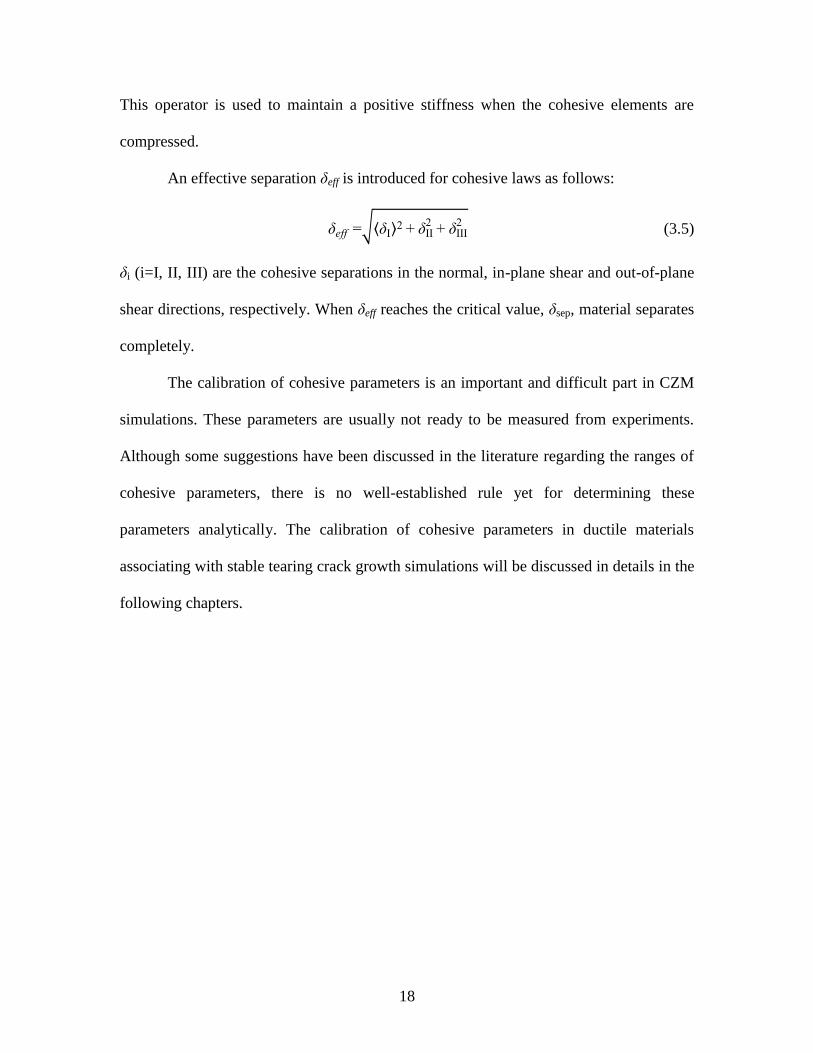
An effective separation δeff is introduced for cohesive laws as follows:
δ √⟨δI⟩ δII δIII
(3.5)
δi (i=I, II, III) are the cohesive separations in the normal, in-plane shear and out-of-plane
shear directions, respectively. When δeff reaches the critical value, δsep, material separates
completely.
The calibration of cohesive parameters is an important and difficult part in CZM
simulations. These parameters are usually not ready to be measured from experiments.
Although some suggestions have been discussed in the literature regarding the ranges of
cohesive parameters, there is no well-established rule yet for determining these
parameters analytically. The calibration of cohesive parameters in ductile materials
associating with stable tearing crack growth simulations will be discussed in details in the
following chapters.

19
CHAPTER 4
BASIC STUDIES ON FINITE ELEMENT MODELING
BASED ON THE MODE I CRACK GROWTH SIMULATIONS
Finite element analysis (FEA) is one of the effective modern techniques to solve
engineering problems. However, depending on complexity of each particular problem,
FEA may introduce numerical factors rather than physical model. Due to less physical
significance, these factors are easily ignored from careful selection and thus lead to
inaccurate predictions. Therefore, before the major simulations of stable tearing crack
growth events in the current study, it is necessary to perform some basic studies on finite
element modeling. These basic studies will be carried out based on the data from the
Arcan test in 2024-T3 aluminum alloy specimen under Mode I loading condition.
The finite element simulations are implemented using ABAQUS, associated with
a custom code in Python extracting results from FE analysis. Simulations are performed
in 3D mesh. As shown in Fig. 4.1 (a), the fixture and specimen are meshed with 8-node
hexahedral elements, C3D8R, while the cohesive zone is meshed with 8-node
quadrilateral cohesive interface elements, COH3D8. A layer of cohesive elements is
placed along the Mode I crack path, starting from the initial straight crack front (note that
the crack is at the left edge of the specimen) to the end of the ligament at the right edge of
the specimen. This layer is along the middle line of the specimen and is surrounded by

20
many small regular elements (seen as a dark band in the mesh). The initial crack length is
6.35 mm. Fig. 4.1(b) shows a zoomed-in view of the mesh with details of the cohesive
interface elements.
(a) (b)
Fig. 4.1 (a) A 3D mesh of the Arcan fixture-specimen system for the Mode I case; (b) a
zoomed-in view of the mesh showing the cohesive interface elements.
In the literature, an explicit scheme (e.g. using ABAQUS/Explicit) is often used
in CZM simulations, even for quasi-static events. But since stable tearing is quasi-static
but explicit analysis is ideally intended for fast dynamic events, the use of
ABAQUS/Explicit requires that artificial acceleration techniques be used. In order for the
results of explicit analysis to be reliable, it must be properly established that the finite
element solution is independent of the particular artificial acceleration values used in the
ABAQUS/Explicit analysis.
On the other hand, ABAQUS/Standard uses implicit time integration schemes and
is ideally suited for quasi-static events. In addition, ABAQUS/Standard takes shorter
computational time than ABAQUS/Explicit to complete for the stable tearing crack

21
growth events. As such, the majority of the simulations in this study are done using
ABAQUS/Standard, except Chapter 6 for the inverse analysis. However, to overcome
numerical convergence problems with material softening introduced in CZM,
ABAQUS/Standard utilizes a viscous regularization technique, which also involves an
artificial viscosity parameter and is needed to be carefully selected.
The load-crack extension curve describes the variation of the load carrying
capability of a cracked specimen or structure with the amount of crack extension during
stable tearing crack growth. Since it is an important curve in structural integrity
evaluations of critical engineering structures such as aircraft structures, this curve is
predicted in the current simulations and will be compared with the experiment.
To determine the location of the crack tip in a CZM based simulation, a consistent
definition of the crack tip is needed. In the literature, several locations, corresponding to
the opening separation δ being equals to 0, δ0 or δsep, have been selected as the crack tip.
To be consistent with the micromechanical process of energy absorption, Shet and
Chandra (2002) suggested that the point coinciding with the peak traction would be the
best choice for the crack tip. For the exponential CZM, Roychowdhury et al. (2002)
defined the crack tip at the location where the opening cohesive stress decreases to 5% of
the peak cohesive traction. Xu and Needleman (1994) reported that simulation
predictions were unaffected when 2δ0 and 5δ0 were selected as the crack tip locations.
On the other hand, to be comparable with the way the crack tip is identified in
experimental measurements, the crack tip in the CZM simulation should be defined as the
point where the separation just reaches the value δsep and the traction is equal to zero.
However, in the experimental measurements, the crack tip was not clearly defined either,

22
since it was determined visually by a person, based on the resolution of the experimental
image and personal best judgment, so experimentally the crack tip may not be exactly at
the location where the material was just separated. Therefore, the crack tip in the CZM
simulation, in the current study, is defined to be the point somewhere in the middle of
each cohesive process, where the separation reaches the value of 0.5δsep.
In the stable tearing experiments by Amstutz et al. (1995), to be simulated in the
current study, the amount of crack extension is the distance traveled by the crack tip from
the initial position to the current position, measured on the outside surface of the
specimen. In the simulations, the amount of crack extension is calculated in the same way
as in the experiments, and the load corresponding to a certain amount of crack extension
is computed by summing the reaction forces at the fixed nodal points in the finite element
mesh that correspond to the location of the fixed loading pin that was held stationary
during experiments.
To gain confidence in the accuracy of the simulation predictions, convergence of
the finite element solutions must be established. In the current chapter, convergence is
investigated with regard to (a) mesh refinement in the specimen thickness direction (an
already fine in-plane mesh in the specimen region, especially along the crack path, is
used), (b) cohesive element length, and (c) viscous regularization, (d) the effects of the
artificial acceleration parameters of the ABAQUS/Explicit solutions.
4.1 Convergence with Mesh Refinement along the Specimen Thickness
The specimen and fixture domains are first divided with a coarse mesh, which,
through the thickness, has one layer of elements in the specimen region and three layers

23
of elements in the fixture region. The cohesive elements have a uniform length of lc = 0.2
mm. To ensure that the finite element mesh is converged, refined meshes are obtained by
bisecting the elements along both the crack path and specimen thickness directions,
respectively. With a sufficiently fine in-plane mesh in the specimen region (especially
along the crack path), the dependence of the simulation prediction of the load-crack
extension curve on the number of element layers through the specimen thickness has
been investigated. Initially, there is only one element layer though the thickness. Then the
number of through-thickness element layers is doubled in each subsequent mesh.
Fig.4.2 Results of convergence check with successive doubling of element layers through
specimen thickness (with cohesive element length = 0.2 mm).
It is found that, with one element though the specimen thickness, either the
simulations are hard to converge or the simulation results are unstable. For some cases,
buckling appears due to the accumulation of computational errors. By bisecting the
elements along the specimen thickness, convergent results (the difference between

24
solutions from two consecutive meshes is less than 1%) are obtained when there are four
layers of elements through the specimen thickness. Fig. 4.2 shows a comparison of the
simulation predictions of the load-crack extension curves from meshes using one through
eight layers of elements through the specimen thickness. It is observed that the load-crack
extension curves corresponding to the meshes with four and eight layers of through-
thickness elements are almost the same. Based on this observation, simulation solutions
with four or more layers of through-thickness elements are considered converged. In the
following study, eight layers of through-thickness mesh is used to simulate Mode I and
mixed-mode I/II stable tearing crack growths.
4.2 Cohesive Element Length
Cohesive element length, h, is a factor that affects both the computational
convergence and the solution accuracy. It is related to the length of the cohesive zone, lcz,
which is defined as a measure of the length over which the cohesive constitutive relation
plays a role (Falk et al., 2001). Numerically a cohesive zone must contain enough number
of cohesive elements in order to capture accurately field variations within and around the
cohesive zone. For various CZM laws, the length of the cohesive zone is expressed by Eq.
(4.1) below, which is summarized in (Turon et al., 2007; Harper and Hallett, 2008):
cz c
(4.1)
where E is the Young’s Modulus of the material, Gc is the critical energy release rate, 0 is
the maximum interfacial strength (denoted as Tmax in the current study), and M is a
parameter that depends on each cohesive model. For linear softening laws (e.g. the
triangular law), M equals to 0.731. lcz is calculated in the range of 1.2 mm to 7.5 mm. To

25
capture the whole cohesive procedure, a sufficient number (e.g. 5 or more) of cohesive
elements are needed within one cohesive zone length. In the current study, cohesive
element length, h, is initially chosen to be 0.2 mm. By bisecting the element length in
subsequently refined meshes along the crack path, h finally equals 0.05 mm in the most
refined mesh.
Fig. 4.3 Results of convergence check with successive bisection of cohesive element
length (with 8 layers of elements through specimen thickness).
Fig. 4.3 shows a comparison of the simulation predictions of the load-crack
extension curves from meshes with h = 0.2 mm, 0.1 mm, and 0.05 mm. It is observed that
the load-crack extension curves corresponding to the meshes with h = 0.1 mm and 0.05
mm are almost the same (the solution difference is less than 1%). Based on this
observation, simulation solutions with h = 0.1 mm or less are considered converged. Thus,
the cohesive element length is fixed at 0.05 mm in the following simulations of Mode I
and mixed-mode I/II stable tearing crack growths.

26
4.3 Viscous Regularization
Since a softening behavior exists in cohesive constitutive laws, simulations using
the CZM approach often encounter numerical difficulties in an implicit solution
procedure (e.g. ABAQUS/Standard). To overcome this problem, various methods have
been proposed, such as the ‘line search’ with a negative step length procedure (Crisfield
et al., 1997) and the modified cylindrical arc-length method (Mi et al., 1998).
Among these methods, two are popular in recent studies in the literature because
of their easy implementation. One of them is to use an explicit procedure (e.g.
ABAQUS/Explicit) instead of an implicit procedure for quasi-static problems in the CZM
approach (e.g. Zavattieri, 2006; Diehl, 2008). The other one is to use viscous
regularization of the constitutive equations assisting with the implicit analysis. This
technique introduces an artificial viscosity factor, which represents the relaxation time of
a viscous system, and causes the tangent stiffness matrix of the softening material to be
positive definite with sufficiently small time increments. The current study employs this
technique available in the ABAQUS/Standard (implicit) solver to improve the
completeness of the solution. Since the viscosity factor is not a physical parameter of
CZM, it is necessary to check the effect of the viscous regularization on the stable tearing
crack growth simulation predictions. Intuitively, when the value of the viscosity
approaches zero, the effect of the artificial viscosity goes to zero. Numerically, this
means that, if the solution is to be considered converged and independent of the viscosity
value, the solution must be associated with a viscosity value that, when it is reduced
properly, the solution does not change significantly. In this study, the values of the
viscosity μ of the cohesive elements are chosen from a set of small values starting from

27
10-3
s and ending at 10-6
s. Each subsequent viscosity value is one-order of magnitude
smaller than the previous one, and the load crack extension response is predicted for each
choice of the viscosity value. The predicted load-crack extension curves are then
compared to seek a convergence trend and thus the choice of the appropriate viscosity
values.
Fig. 4.4 Load-crack extension curves with various viscosity values for the cohesive
elements.
It is shown in the Fig. 4.4 that, the predicted load-crack extension curve is
dependent on the selection of the viscosity value until the viscosity value becomes
sufficiently small. In particular, when the viscosity value changes from 10-4
to 10-5
s and
then to 10-6
s the simulation results tend to overlap with each other and become
independent of the choice of the viscosity value and hence can be considered converged.
It is worth noting that the choice of the viscosity value (in the range explored in the
current study) does not affect the cost of the CPU time. Thus, the viscosity value in the

28
current study is set to be 10-6
s, which is different from the suggested value in the
ABAQUS manual.
As an independent check of the solution convergence for the choice of the
viscosity value chosen, a custom FEM code, CRACK3D, was also employed to perform
the same simulations using the same CZM model. In CRACK3D, the triangular CZM is
implemented without using the viscous regularization technique, and hence there is no
need to specify the viscosity (thus the viscosity is considered to be zero in CRACK3D).
In ABAQUS, μ is set to equal the convergent value, 10-6
s, which is the value nearest to 0
in the range of values explored in this study. It is noted that, although CRACK3D does
not need an artificial viscosity value, it does take a much longer computing time
compared to ABAQUS to get a solution. For the comparison, to minimize the time need
for CRACK3D simulations, two relatively coarse meshes with two sets of CZM
parameter values are employed (the choice of the CZM parameter values for the
comparison simulations is not significant). The first mesh has two layers of through-
thickness elements and a cohesive element length of 0.15 mm, with CZM parameter
values of Tmax = 621 MPa, δ0 = 0.01 mm and δsep= 0.055 mm. The second mesh has four
layers of through-thickness elements and a cohesive element length of 0.2 mm, with
CZM parameter values of Tmax = 759 MPa, δ0 = 0.0078 mm, and δsep = 0.0448 mm. The
comparison shown in Fig. 4.5 reveals that, for each comparison group, the load-crack
extension curves predicted from simulations using ABAQUS/Standard and using
CRACK3D match very well , thus demonstrating that the ABAQUS/Standard simulation
results with μ =10-6
s are converged and reliable.

29
Fig. 4.5 Comparison of results from ABAQUS (μ =10-6
s) and CRACK3D for two cases
(Case 1: mesh1, 2-layer mesh with h = 0.2 mm, Tmax = 621 MPa, δ0 = 0.01 mm, δsep =
0.055 mm; Case 2: mesh2, 4-layer mesh with h = 0.15 mm, Tmax = 759 MPa, δ0 = 0.0078
mm, δsep = 0.0448 mm).
4.4 Convergence Issues in Simulations of Stable Tearing Crack Growth with the
CZM Approach Using an Explicit Analysis Procedure
An explicit solution procedure (e.g. in ABAQUS/Explicit) is often used in the
simulations using CZM approach. However, since explicit solution procedures, which
employ a large number of small increments, are usually intended for fast dynamic events
with short durations, simulations of slow quasi-static events, such as stable tearing crack
growth, will require a very long computational time. Thus practical simulations of quasi-
static events often necessitate the use of artificial acceleration techniques. For example, in
ABAQUS/Explicit, simulations of quasi-static events can be accelerated by either
speeding up the application of loading or scaling up the mass of the material. However,

30
without a careful selection of the analysis parameter values used in the techniques, an
artificially increased inertia force can lead to inaccurate results, although a complete
solution can be reached. Therefore, the choice of the analysis parameter values in the
explicit procedure is very important but is barely discussed in the literature. To this end,
the simulations of stable tearing crack growth in Mode I Arcan test using the CZM
approach are carried out in this section with the ABAQUS/Explicit solver, aiming at
finding a way of setting analysis parameter values for a reliable prediction. The
convergent mesh described in Section 4.1- 4.2 is used for the explicit analysis. The set of
CZM parameter values (Tmax = 759 MPa, δ0 = 0.0078 mm and δsep = 0.0448mm) obtained
from the simulations of Mode I Arcan test with the implicit procedure in
ABAQUS/Standard, leading to a good predictions of stable tearing crack growth events
for both Mode I and mixed-mode I/II loading conditions (see Chapter 5) will be
employed in this section for the explicit analysis. For reference, predictions from the
implicit procedure as well as the experimental measurements are compared.
An explicit analysis performs a large number of small time increments. In each
increment, δt, the calculation proceeds without iterations and without requiring the
tangent stiffness matrices to be formed. In ABAQUS/Explicit, the analysis employs the
central-difference operator, and the time increment must be smaller than the stability
limit of this operator to avoid unstable solution. Generally, there are two ways to estimate
the time increment, δt. One is based on the element-by-element stability estimate, which
can be written as (ABAQUS Manual 6.10):
√
(4.2)

31
where the minimum is taken over all elements in the mesh, Le is a characteristic length
associated with an element, ρ is the density of the material in the element, and and
are the effective Lame’s constants for the material in the element. The other way is based
on the global stability estimate. The time increment from the global estimate may be
somewhat larger. If δt remains constant, the number of increments, n, is
n =T/δt (4.3)
where T is the time period of the event being simulated.
Comparing with the implicit procedure, the time period in an explicit analysis has
more physical meanings. Generally, it corresponds to the real event time, T0, particularly
for a rate-dependent response. For quasi-static simulations, the generally very long real
event time leads to an extremely large CPU cost, since the computer time involved in the
explicit time integration with a given mesh is proportional to the time period of the event.
In Mode I Arcan test, the rate of the quasi-static displacement loading is 2.54×10⁻³
mm/s
(10-4
inch/s). If the total displacement loading in the simulation is 1 mm, then the real
event time, T0, of the quasi-static test is around 393s. If the time increment is on the order
of 10-9
s, then the required CPU cost for a real event time of T0 = 393 s will be enormous
and it will be impractical and prohibitive to perform the simulations with this cost.
To achieve an economical solution, two approaches can be used in ABAQUS/
Explicit either separately or in combination: (a) artificially accelerate the event by
reducing the time period of the analysis and (b) artificially accelerate the event by
increasing the mass density of the model (mass scaling). The experience from the current
study in using these two techniques for efficient and accurate simulations of stable
tearing crack growth events are presented below.

32
4.4.1 Reduce the Time Period
To reduce the number of increments required, n, and speed up the simulations, we
can reduce the time period of the analysis, T, compared to the total real event time of the
actual process, T0. However, if the simulation is accelerated too much, the increased
inertia forces will change the predicted response. To understand the convergence property
of the load-crack extension curve, simulations are carried out with a time period of 0.01 s
(which corresponds to about 5 times of the basic frequency of the system) and repeated
by doubling the time period subsequently, without changing the default values of other
analysis factors, such as the time increment δt. The total displacement loading in the
simulation is 1.0 mm.
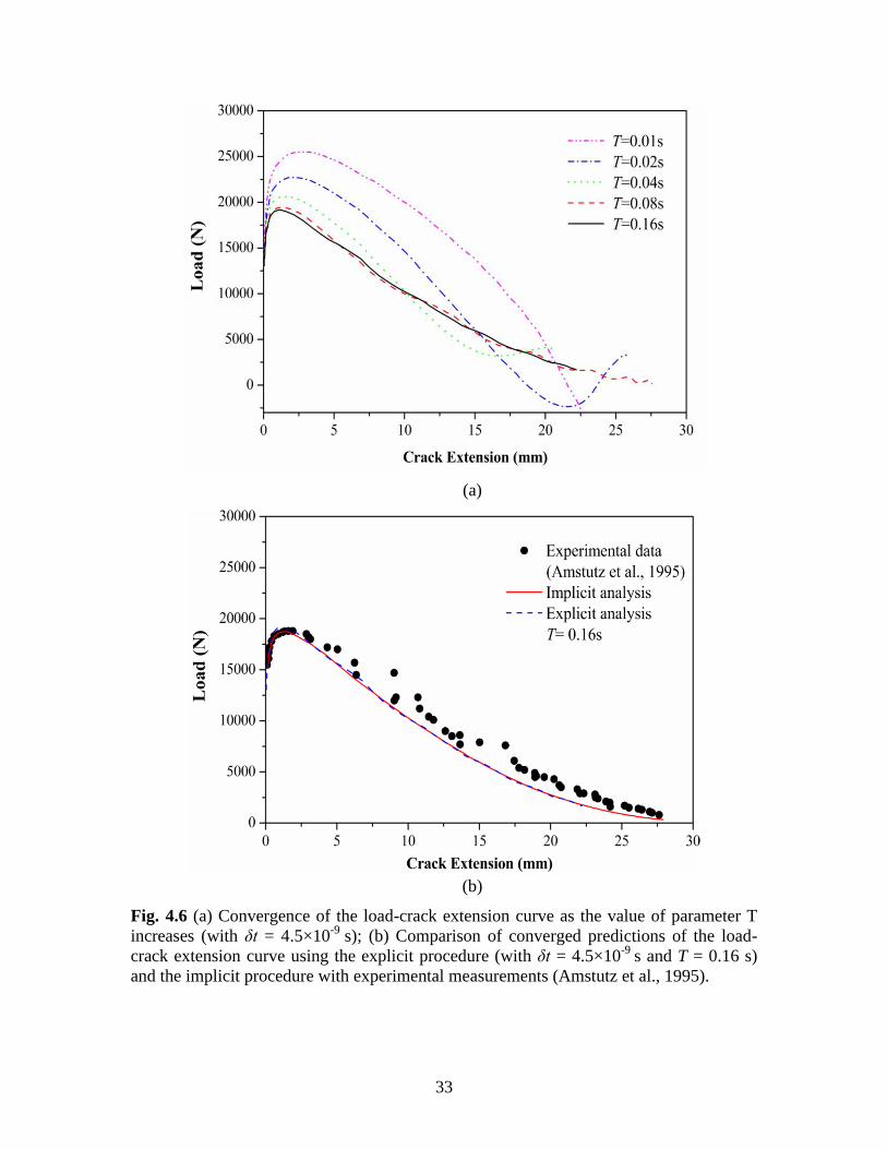
The results of the predicted load-crack extension curves calculated using different
period time are plotted in Fig. 4.6. It is shown in Fig. 4.6 (a) that, when the time period, T,
is too short relative to the actual total event time, T0, the accuracy of the predicted results
is bad (e.g. the predicted peak load is too large relative to the experimental value). As T
increases, the accuracy of the predicted results is better (e.g. the predicted peak load
decreases and becomes closer to the experimental value). Converged predictions of the
load-crack extension curve are observed when T increases from 0.08 s to 0.16s. Although
the time period of T = 0.16s is still far smaller than the actual event time, T0 (which is 393
s), the converged prediction of the load-crack extension using the explicit procedure
(with a computational speed up of nearly 2,500) is almost the same as that using the
implicit procedure and compares well with experimental measurements (see Fig. 4.6 (b)).
33
(a)
(b)
Fig. 4.6 (a) Convergence of the load-crack extension curve as the value of parameter T
increases (with δt = 4.5×10⁻⁹
s); (b) Comparison of converged predictions of the load-
crack extension curve using the explicit procedure (with δt = 4.5×10⁻⁹
s and T = 0.16 s)
and the implicit procedure with experimental measurements (Amstutz et al., 1995).

34
4.4.2 Mass Scaling
Another way to shorten the analysis time of the explicit simulation is using the
mass scaling technique to artificially increase the material density by a factor, say f 2.
Based on Eq. (4.2) and (4.3), this technique reduces the number of time increments, n, to
n/f, which is equivalent to decreasing the time period, T, to T/f. However, at the same
time of decreasing the analysis time, the accuracy of the predictions may be degraded by
the effect of the artificial inertia forces. Thus, convergence of simulation predictions must
be established so that the predictions are not strongly affected by the use of the artificial
technique. Since the actual event time of the Arcan test is very long, an extremely large
mass scaling factor is needed to make sure a reasonable analysis time can be achieved,
which is not easy to handle with. Therefore, two alternative series of simulations using a
combination of reducing the time period and increasing the mass of system are performed
to understand the convergence property of the predictions.
In the first series of simulations, the time period of analysis is fixed at 1.0 s (with
a total displacement of 0.5 mm), and the value of the mass scaling parameter f 2 is chosen
to be 50,000, then 5,000, then 500, and finally 50. Apparently, the larger the mass scale
factor is, the shorter time the analysis will take (computation time varies from several
days to several hours). As shown in Fig. 4.7(a), when f 2
is too large relative to 1 (e.g.
50,000), the predicted peak load is too large relative to the experimental value; and when
f 2
becomes smaller, the predicted peak load becomes smaller and closer to the
experimental value. Convergence of the predicted load-crack extension curve is observed
when f 2
is decreased from 500 to 50. The converged prediction of the load-crack
extension using the explicit procedure (with a computational speed up of nearly 1,750) is

35
almost the same as that using the implicit procedure and compares well with
experimental measurements (see Fig. 4.7 (b)).
(a)
(b)
Fig. 4.7 (a) Convergence of the load-crack extension curve as the value of parameter f 2
decreases (with T=1s and δt =4.0×10⁻⁸
s); (b) Comparison of converged predictions of the
load-crack extension curve using the explicit procedure (with T=1 s, δt =4.0×10⁻⁸
s and f 2
=50) and the implicit procedure with experimental measurements (Amstutz et al., 1995).

36
(a)
(b)
Fig.4.8 (a) Convergence of the load-crack extension curve as the value of parameter T
increases (with f 2
= 50,000 and δt =1.25×10⁻⁶
s); (b) Comparison of converged
predictions using the explicit procedure (with T = 32 s, δt =1.25×10⁻⁶
s and f 2
=50,000)
and the implicit procedure with experimental measurements (Amstutz et al., 1995).
37
In the second series of simulations, the mass scalar factor is fixed at 50,000, and
the time period, T, takes the value of 1 s, 2 s, 4 s, 8 s, 16 s, or 32 s (the total displacement
is 0.5 mm). As shown in Fig. 4.8. (a), when T is too small (e.g. 1 s) relative to the actual
even time, the predicted peak load is too large relative to the experimental value; and
when T is increased, the predicted peak load is decreased and gets closer to the
experimental value. Convergence of the predicted load-crack extension curve is observed
when T is increased from 16 s to 32 s. The converged prediction of the load-crack
extension using the explicit procedure (with a computational speed up of nearly 1,700) is
almost the same as that using the implicit procedure and compares well with
experimental measurements (see Fig. 4.8 (b)).
4.4.3 Summary
Based on the above results, three sets of artificial acceleration parameter values in
the explicit procedure are found to produce converged predictions of the load-crack
extension curve with good agreement with predictions using the implicit procedure and
with experimental measurements. These sets of values are listed in Table 4.1. In the table,
the displacement loading per time increment, d, can be calculated by
Dd t
T (4.4)
where D is the total displacement loading. As shown in Table 4.1, when d is on the order
of 10-8
mm, the predictions converge. In light of this observation, other mass scaling
values could be applied to obtain converged predictions as long as the displacement per
time increment is properly small (e.g. on the order of 10-8
mm in this study). In the
current simulation, if the total displacement is 1mm, and the time period is kept at 1s,
then the time increment should be on the order of 10-8
s to ensure convergence. To
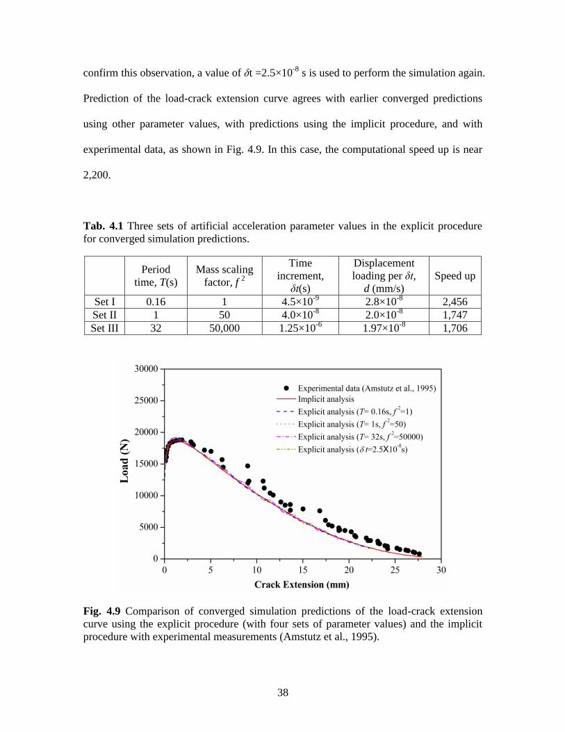
38
confirm this observation, a value of δt =2.5×10⁻⁸
s is used to perform the simulation again.
Prediction of the load-crack extension curve agrees with earlier converged predictions
using other parameter values, with predictions using the implicit procedure, and with
experimental data, as shown in Fig. 4.9. In this case, the computational speed up is near
2,200.
Tab. 4.1 Three sets of artificial acceleration parameter values in the explicit procedure
for converged simulation predictions.
Period
time, T(s)
Mass scaling
factor, f 2
Time
increment,
δt(s)
Displacement
loading per δt,
d (mm/s)
Speed up
Set I 0.16 1 4.5×10⁻⁹
2.8×10⁻⁸
2,456
Set II 1 50 4.0×10⁻⁸
2.0×10⁻⁸
1,747
Set III 32 50,000 1.25×10⁻⁶
1.97×10⁻⁸
1,706
Fig. 4.9 Comparison of converged simulation predictions of the load-crack extension
curve using the explicit procedure (with four sets of parameter values) and the implicit
procedure with experimental measurements (Amstutz et al., 1995).

39
To summarize, by properly adjusting the time period, the mass scaling factor and
the time increment, a significant reduction in CPU cost can be achieved in explicit
simulations of stable tearing crack growth events without losing accuracy. Consequently,
for the cases in which the implicit solver meets numerical difficulties in convergence, the
explicit solver can be utilized confidently to reach complete and accurate solutions. In
addition, for the particular problem discussed in the current study, the two acceleration
techniques are identical, which is not hard to tell from Eq. 4. and 4.3 . The
convergence study aims at reducing the computation time but not inducing significant
inertia effects. An enough time is needed to ensure stress wave spreads out the
information well through the system so that to maintain static equilibrium in each load
increment. However, one has to be careful if the physical problem is expected to become
unstable e.g. the crack becomes unstable and there is a true dynamic transient . Then the
method presented in section 4.4.1 reduce the time period is preferred to capture the true
dynamic behavior. Artificially increase the density would not yield realistic results if
dynamic behavior e.g. dynamic crack propagation becomes important. In contrast, mass
scaling is more used for reducing the solution time in simulations involving a rate-
dependent material or rate-dependent damping.

40
CHAPTER 5
SIMULATIONS FOR MIXED-MODE I/II
STABLE TEARING CRACK GROWTH EVENTS
5.1 Validation of CZM on Mode I Crack Growth Events
After the studies of basic issues discussed in Chapter 4, the converged mesh with
eight layers of through-thickness elements, a cohesive element length of 0.05 mm is fixed
and will be used to simulate both Mode I and mixed-mode I/II stable tearing crack
growths. In the current chapter, simulations will be carried out using ABAQUS/Standard,
with the choice of viscosity μ equals to 10-6
s. A 3D mesh of the Arcan fixture-specimen
system for the Mode I case is shown in Fig. 4.1.
To calibrate the cohesive parameters, some suggestions were found in the
literature. It is generally accepted that the cohesive energy equals the fracture energy
of the material, c. Thus,
δsep c / max (5.1)
The value of c for 2024-T3 aluminum alloy has been suggested in the literature.
In the analysis of energy balance for a double edge notched plate of 2024-T3 aluminum
alloy, Shet and Chandra (2002) let c equal to the critical plane strain value of the J-
integral, JIC=8 KJ/m2. On the other hand, Li and Siegmund (2002) set c to 17 KJ/m
2 for
an exponential CZM, which is calculated from the stress intensity factor based initial

41
fracture toughness value of KIC=35 MPam1/2
(Haynes and Gangloff, 1997) for 2024-T3
aluminum alloy thin sheet specimens.
The value of the cohesive strength Tmax for various cohesive laws has been
estimated mostly based on the initial yield stress σy of the material surrounding the
cohesive zone and sometimes based on the ultimate tensile strength σu. In the reference,
Li and Siegmund (2002) summarized that the ratio Tmax/σy ranges from 1.2 to 4 for
different conditions and they chose 2σy as the cohesive strength in their models.
Roychowdhury et. al. (2002) set Tmax equal to 2.7σy to analyze ductile tearing in thin
aluminum panels under large displacement. In reference (Cornec et al., 2003), Tmax is
determined based on σu to simulate fracture in C(T) specimens made of 2024-T351
aluminum alloy in tension tests.
The initial cohesive stiffness K or the characteristic normal separation δ0 should
be chosen so that K>>E/L (Turon et al., 2007) (where E is the Young’s modulus of the
specimen and L is the dimension of the specimen) to ensure that the overall structural
stiffness or compliance of the specimen is not affected by the presence of CZM interface
elements. In particular, the characteristic normal separation δ0 can be chosen based on (Li
and Siegmund, 2002; Shet and Chandra, 2002) using
c = eTmaxδ0 (5.2)
where e=exp(1), which is based on the relations among c, Tmax and δ0 for an exponential
cohesive law. The specific value of δ0 or K will be given in the next section.
In the current study, the cohesive parameter values for TL oriented specimens
made of aluminum alloy 2024-T3 will be selected based on the values used in the
literature, through matching the simulation prediction of the Mode I load-crack extension

42
curve with experimental data. The cohesive energy in the current study is taken to be 17
KJ/m2, the value used in (Li and Siegmund, 2002; Haynes and Gangloff, 1997). The
cohesive strength Tmax is chosen from the range of 1.0σy to 4.0σy, while δsep is computed
from Eq. (5.1) and δ0 is computed from Eq. (5.2) (provided the resulting K computed
from Eq. (3.1) satisfies K>>E/L).
5.1.1 Effect of Tmax and δsep
In order to understand how the simulation prediction of the load-crack extension
curve will be affected by the choice of Tmax or δsep, a range of simulations have been
carried out using various values of Tmax or δsep, while other CZM parameters are fixed.
For example, Fig. 5.1 shows the simulation predictions of the load-crack extension curve
for various values of Tmax, when δ0 = 0.0078 mm and δsep = 0.0448 mm. It can be
observed from the figure that, the peak value of the load, which is the maximum residual
strength the specimen against stable tearing, is higher when Tmax is larger. It is also found
that when Tmax is less than 1.5σy (recall σy = 345 MPa), an unstable crack growth behavior
happens. Similarly, it is shown in Fig. 5.2 that, when Tmax and δ0 are fixed, a larger value
of δsep will lead to a higher peak value of the load.
Computationally, it is noticed that, when Tmax or δsep is smaller, the computing
time is shorter; when the value is even smaller (e.g., Tmax is less than σy), the increasing
part of the load-crack extension curve will vanish. On the other hand, when Tmax or δsep is
very large (e.g., Tmax is larger than 4σy), the analysis is hard to complete due to numerical
difficulties even though the viscous regulation technique is used.
Since the cohesive energy is always considered as an important parameter of
CZM, simulations are carried out again with various values of Tmax when c is kept

43
constant (δsep and δ0 are computed from Eqs. (5.1) and (5.2)). However, Fig. 5.3 shows
that the predicted load-crack extension curve is higher when Tmax is larger. This result
indicates that predictions do depend on other cohesive parameters even if the cohesive
energy does not change.
Fig. 5.1 Load-crack extension curves for various Tmax values when δ0 and δsep are fixed.
Fig. 5.2 Load-crack extension curves for various δsep values when Tmax and δ0 are fixed.

44
Fig. 5.3 Load-crack extension curves for various Tmax values when c is fixed.
The above observations are useful in selecting proper CZM parameter values for
the current study. The final choice of the CZM parameter values will be determined by
matching simulation prediction of the Mode I load-crack extension curve with
experimental measurements, with consideration of the CZM parameter values used in the
literature.
5.1.2 Final Choice of CZM Parameter Values and Comparisons with Experimental Data
A series of simulations of the Mode I stable tearing crack growth have been
carried out using various CZM parameter values. Simulation predictions of the load-crack
extension curve are compared with experimental measurements. After a range of trials, a
proper set of CZM parameter values is found: Tmax = 2.2σy = 759 MPa, δ0 = 0.0078 mm
and δsep = 0.0448 mm. Simulation prediction of the load-crack extension curve, using this
set of CZM parameter values, is compared with experimental measurements in Fig. 5.4. It
is seen that the CZM simulation prediction of the load-crack extension agrees well with

45
the experimental data from the start of the curve to the peak load (which is the most
important quantity from the load-crack extension curve). Beyond the peak load, the
predicted load somewhat under-estimates the experimental value.
Fig. 5.4 Comparison of Mode I load-crack extension curves from experimental
measurements (Amstutz et al., 1995) and from simulation predictions using CZM (Tmax =
759 MPa, δ0 = 0.0078 mm, δsep = 0.0448 mm) and using CTOD (Lan et al., 2007).
The prediction of the load-crack extension curve has often been made using a
fracture criterion based on the crack tip opening displacement (CTOD) (Ma et al., 1999;
Sutton et al., 2000). In the CTOD criterion, crack growth occurs when CTOD at a certain
distance behind the crack front reaches a critical value. In comparison, in the CZM
approach, crack growth occurs when the cohesive element ahead of the crack front is
sufficiently damaged and can no longer support any traction. In the case of the Mode I
stable tearing crack growth in an Arcan specimen, good agreement between experimental
data and simulation predictions based on the CTOD criterion have been demonstrated
using both a 2D model (Deng and Newman, 1999) and a 3D model (Lan et al., 2007),

46
which employ a critical CTOD value determined from experimental measurements of
CTOD variations with crack extension (Amstutz et al., 1995). The simulation prediction
using the CTOD approach (Lan et al., 2007) is also shown in Fig. 5.4. The CZM and
CTOD approaches lead to almost the same predictions, showing good agreement with the
experimental data for the peak load.
At this time it is not clear why the predicted load beyond the peak load has a
larger difference with the experimental measurements. One reason for this larger
difference may be the use of simplifications in the finite element model of the specimen-
fixture system. For example, the bolted connection between fixture and specimen is
assumed to be a continuous, perfectly bonded connection; the loading pin holes are not
represented in the FEM; and the surface load that is transferred from the loading pins to
the pin hole walls through bearing contact is simplified as a line of displacement loading
at a line of finite element nodes through the specimen thickness. Errors due to these
simplifications will tend to be larger at later stages of crack growth when the specimen-
fixture system experiences larger overall deformation and rotation. Another reason for
this under-estimation in both the CZM and CTOD based simulations, which is common
in published simulations (not just by the current authors), may be that these simulations
assume constant CZM parameter values or a constant critical CTOD value , while in
reality these values may be stress-state dependent.
5.1.3 Variation of CTOD with Crack Extension
As an immediate validation of the CZM simulation prediction using the set of
CZM parameter values chosen based on matching the load-crack extension curve, the
simulation predicted variation of the CTOD at a certain fixed distance behind the moving
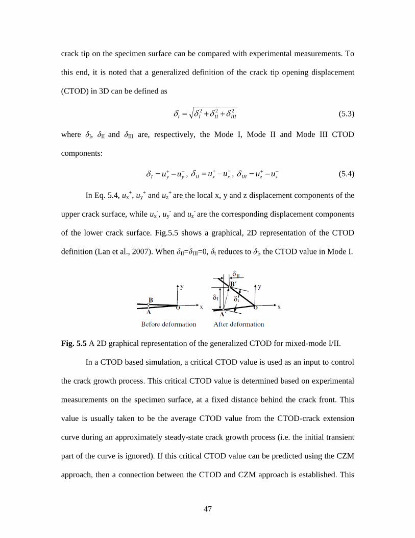
47
crack tip on the specimen surface can be compared with experimental measurements. To
this end, it is noted that a generalized definition of the crack tip opening displacement
(CTOD) in 3D can be defined as
222
IIIIIIt (5.3)
where δI, δII and δIII are, respectively, the Mode I, Mode II and Mode III CTOD
components:
yyI uu , xxII uu , zzIII uu (5.4)
In Eq. 5.4, ux+, uy
+ and uz
+ are the local x, y and z displacement components of the
upper crack surface, while ux-, uy
- and uz
- are the corresponding displacement components
of the lower crack surface. Fig.5.5 shows a graphical, 2D representation of the CTOD
definition (Lan et al., 2007). When δII=δIII=0, δt reduces to δI, the CTOD value in Mode I.
Fig. 5.5 A 2D graphical representation of the generalized CTOD for mixed-mode I/II.
In a CTOD based simulation, a critical CTOD value is used as an input to control
the crack growth process. This critical CTOD value is determined based on experimental
measurements on the specimen surface, at a fixed distance behind the crack front. This
value is usually taken to be the average CTOD value from the CTOD-crack extension
curve during an approximately steady-state crack growth process (i.e. the initial transient
part of the curve is ignored). If this critical CTOD value can be predicted using the CZM
approach, then a connection between the CTOD and CZM approach is established. This

48
point will be discussed in detail in Section 5.2 when the CZM approach is used to
simulate stable tearing crack growth events under mixed-mode I/II conditions, using the
same set of CZM parameters determined from the Mode I case.
Fig. 5.6 For Mode I case, comparison of CZM prediction of the variation of CTOD at 1
mm behind the crack tip with crack extension with experimental measurements (Amstutz
et al., 1995).
In the current study, since the distance of 1.0 mm behind the crack tip was used in
the experimental measurement of CTOD, this distance is also employed in the
simulations when CTOD is computed. In Fig. 5.6, with the CZM approach, the
simulation prediction of the CTOD variation with crack extension for the Mode I case is
compared with experimental measurements. It is seen that the predicted CTOD variation
lies within the range of the experimental data. Overall, it is reasonable to state that the
simulation prediction compares well with the experimental measurements, thus validating
the CZM simulation results using the set of CZM parameter values determined from
matching the Mode I load-crack extension curve.

49
5.1.4 Crack Tunneling
Crack tunneling has been commonly observed in stable tearing crack growth
experiments on specimens made of ductile materials, which can be attributed to
variations of the stress constraint (also called the stress triaxiality, defined as the ratio of
the hydrostatic stress with the von Mises effective stress) with distance to specimen
surface (e.g. Zuo et al., 2008). For a through-thickness crack, the crack front will meet
the “fracture criterion” first at the mid-thickness region and then at points towards the
specimen surface, leading to a “thumbnail” shaped crack front. To develop a 3D fracture
criterion for general stable tearing crack growth in ductile material, a proper
understanding of this fracture behavior is important. Based on experimental results and
analyses of CTOD/CTOA along the crack front, the crack tunneling phenomenon has
been discussed in (James and Newman, 2003; Zuo et al., 2008). The studies by Zuo et al.
(2008) and Lan et al. (2010) indicate that full 3D predictions of crack growth events
based on a CTOD criterion should consider the effects of stress-state parameters such as
the stress constraint since the fracture toughness in terms of a critical CTOD is in general
not a constant along the crack front.
In the current study, it is noted that crack tunneling is predicted by the CZM
simulations when the same set of CZM parameter values is used for all cohesive interface
elements (i.e. possible stress-state dependence of CZM parameter values is not
considered). In the simulations, cohesive elements ahead of the crack front reach the
maximum traction and maximum separation first in the mid-thickness region.
Consequently, crack growth occurs earlier in the mid-thickness region than near the
outside surfaces of the specimen, leading to crack tunneling.

50
Fig. 5.7 shows the variations of the tunneled crack front profiles at various stages
of crack extension, and how the tunneled shape is affected by Tmax or δsep. The predicted
shape of the tunneled crack front is smoothed using the spline function. It is observed that
crack tunneling is strongly affected by the value of Tmax (tunneling is severer when Tmax is
higher) and is almost not affected by the value of δsep except when the amount of crack
extension is small (see Fig. 5.7(d)). It is also observed that the severity of crack tunneling,
from an initially straight crack front to a tunneled crack after crack growth, increases
quickly at the earlier period of crack growth and then it stays steady as crack growth
continues, which is consistent with experimental observations (e.g. Dawicke and Sutton,
1994; Roychowdhury et al., 2002). Although there are no quantitative measurements of
crack front shapes on these Arcan specimens for direct comparison, the predicted shapes
of the crack front are very similar to those from qualitative observations on fracture
surfaces after the experiments.
Due to crack tunneling and the influence of crack tunneling on the near crack
front stress distributions, CZM simulations (with the same CZM parameter values) using
a 2D model and 3D models with various numbers of layers of through-thickness elements,
all with the same CZM parameter values, may lead to different simulation predictions.
Based on the results of this study, 3D models with a sufficient number of through-
thickness layers of elements are expected to give the most accurate predictions because
they allow the crack front to evolve and converge based on the given cohesive law.

51
(a) (d)
(b) (e)
(c) (f)
Fig. 5.7 Effect of Tmax , δsep and crack extension on the variation of crack front profile: (a),
(b) & (c), effect of Tmax; (d), (e) & (f), effect of δsep; (a) & (d), crack front profile when
crack extends to 0.15 mm on the front surface of the specimen; (b) & (e) crack front
profile when crack extends to 19.75 mm on the front surface of the specimen; (c) & (f)
crack front profile when crack extends to 25.05 mm on the front surface of the specimen.
52
5.2 Simulations for Mixed-mode I/II Stable Tearing Crack Growth Events
In engineering applications, fracture often occurs under mixed-mode loading
conditions. An extension of CZM law into mixed-mode cases was introduced in Section
3.2. In this section, the triangular cohesive law is further applied to investigate the
simulations of mixed-mode I/II stable tearing crack growth events in Arcan specimens
made of 2024-T3 aluminum alloy (Amstutz et al., 1995) involve curvilinear crack paths
(see Fig. 5.8). To avoid complications due to the need to predict the crack path, CZM
simulations in this study will utilize finite element models with a prescribed crack path
that is determined experimentally. The CZM mixed-mode simulations are thus focused
on the predictions of the load-crack extension curve and the variation of the CTOD with
crack extension and on the experimental validation of the simulation predictions. Two
mixed-mode cases will be considered: the 15° and 45° loading cases.
For the simulation of mixed mode I/II stable tearing crack growth, the two
cohesive parameters Tmax and δsep, are chosen as the input parameters in the simulations.
In the current study, the cohesive strength is assumed to be the same for both Mode I and
mixed-mode I/II cases. In general, the fracture toughness is often higher in Mode II (e.g.
due to crack surface contact and friction in stable tearing crack growth) than in Mode I,
and as such, CZM parameter values from Mode I alone are often not sufficient for mixed-
mode cases. However, for stable tearing crack growth events that are locally Mode I at
the crack front, Mode II contributions in the CZM are expected to be small, and for such
cases, it is believed that using the CZM parameter values from Mode I will not lead to
significant errors in simulation predictions for this type of mixed-mode I/II cases. To this
end, two mixed-mode stable tearing crack growth events that are locally Mode I are

53
simulated in this study. The same set of CZM parameter values for the triangular
cohesive law chosen based on the Mode I case will be employed for these mixed-mode
I/II simulations.
5.2.1 FE Model for Mixed-mode I/II Cases
Convergence practices regarding element size for through-thickness elements and
cohesive elements and for the viscosity value will be carried over from the Mode I case to
the mixed-mode cases. The same set of CZM parameter values for the triangular cohesive
law chosen based on the Mode I case will be employed for the mixed-mode I/II
simulations. Thus the only difference between the Mode I finite element model and the
mixed-mode I/II finite element models is that the crack path in Mode I is straight and
those in the mixed-mode cases are curvilinear. Using the experimentally measured crack
propagation paths in the mixed-mode Arcan tests (Amstutz et al., 1995), the x, y values
of the crack paths for the 15° and 45° loading cases are fitted to smooth lines (Fig. 5.8).
Fig. 5.8 Experimentally measured (symbols) and numerically smoothed (lines) crack
paths for the 15° and 45° mixed-mode I/II Arcan tests (Amstutz et al., 1995). The
smoothed crack paths are predefined in simulations so that crack direction prediction is
not needed.

54
Fig. 5.9 A frontal view of the 3D mesh for the 45° loading case.
Displacement loading is applied by fixing the set of nodes on one grip pin and moving
the set of nodes on the other grip pin at the opposite end of the radial loading line (see Fig.
2.1(a)). A frontal view of the 3D mesh for the 45° loading case is shown in Fig. 5.9.
5.2.2 Simulation Predictions and Validation by Experimental Data
CZM simulation predictions of the load-crack extension curve and the CTOD
variation with crack extension will be presented and compared with experimental data.
Figs. 5.10 and 5.11 show the load-crack extension curves for the 15° and 45° loading
cases, respectively. It is seen that the CZM simulation predictions for both mixed-mode
I/II cases are in good agreement with experimental data, especially for the most important
quantity, the peak load in the load-crack extension curve. For comparison, the predictions
by Lan et al. (2007) using a CTOD based simulation are also shown. For the 45° loading
case, the CZM and CTOD simulation predictions are almost the same and they almost
overlap with the experimental curve except near the tail end of the curve. For the 15°
loading case, the CZM simulation slightly under-predicts the peak load and the CTOD
simulation somewhat over-predicts the peak load; and the CTOD simulation prediction in

55
the part of the curve beyond the peak load is in better agreement with experimental
measurements than the CZM simulation prediction.
Fig. 5.10 Comparison of load-crack extension curves from experimental measurements
(Amstutz et al., 1995) and from simulation predictions using CZM (Tmax = 759 MPa and
δsep = 0.0448 mm) and using CTOD (Lan et al., 2007) for the 15° loading case.
Fig. 5.11 Comparison of load-crack extension curves from experimental measurements
(Amstutz et al., 1995) and from simulation predictions using CZM (Tmax = 759 MPa and
δsep = 0.0448 mm) and using CTOD (Lan et al., 2007) for the 45° loading case.

56
Another important quantity predicted by the CZM simulation is the CTOD
variation with crack extension at a fixed-distance behind the moving crack tip on the
specimen surface. To compare with experimental data, this fixed distance is chosen to be
1 mm which is the distance used in the experimental measurements. The CZM simulation
predictions are shown in Figs. 5.12 and 5.13 for the 15° and 45° loading cases,
respectively, along with the experimental data. It is clear from the figures that, for each
mixed-mode I/II loading case, the predicted CTOD values are located within the range of
the experimental measurements.
Fig. 5.12 For the 15° mixed-mode I/II case, comparison of CZM prediction of the
variation of CTOD at 1 mm behind the crack tip with crack extension with experimental
measurements (Amstutz et al., 1995).

57
Fig. 5.13 For the 45° mixed-mode I/II case, comparison of CZM prediction of the
variation of CTOD at 1 mm behind the crack tip with crack extension with experimental
measurements (Amstutz et al., 1995).
To summarize the CTOD prediction results and gain a better understanding of the
comparisons between the CZM simulation predictions and experimental measurements,
the simulation predictions and experimental measurements for the two mixed-mode I/II
loading cases as well the Mode I loading case are shown together in Fig. 5.14. It is seen
that the predicted and measured CTOD variations are in good agreement with each other
and that the CTOD value is higher initially and then stabilizes to a more or less constant
mean value after an initial stage of crack extension. This mean value can be calculated by
averaging the CTOD values for crack extensions greater than, say, 7.0 mm. It is worth
noting that in CTOD based simulations this average CTOD value from experimental
measurements is taken to be the critical CTOD value in a CTOD fracture criterion and
used as an input in the simulations. For example, in the CTOD simulations by Lan et al.

58
(2007), the critical CTOD value is taken to be the average value of CTOD measurements
for crack extensions greater than 10.0 mm. Fig. 5.14 shows that the average CTOD
values for crack extensions greater than 10.0 mm, from both the experimental
measurements and the CZM simulation predictions, are identical and equal to 0.078 mm.
Fig. 5.14 Comparison of predicted and measured CTOD variation with crack extension
under mode I and mixed-mode I/II conditions. The average CTOD value is 0.078 mm for
both experiment and prediction, which is the average of the CTOD values for crack
extensions greater than 10.0mm beyond which the CTOD variation oscillates around the
average value.
Comparisons shown above provide strong experimental validations for the mixed-
mode CZM simulation predictions of the load-crack extension curve and of the CTOD
variation with crack extension. It is important to note that the same CZM parameter
values determined from Mode I experimental data are used for the mixed-mode
simulations. The fact that CZM based simulations can predict the critical CTOD value
that is normally determined from experimental data and used as input in CTOD based
simulations speaks volumes about the existence of a strong connection between the CZM

59
and CTOD based approaches for stable tearing crack growth simulations. This connection
also explains why the predicted load-crack extension curves using the two approaches
have close agreement with each other.
5.3 Summary
A cohesive zone model (CZM) based approach has been successfully applied to
simulate both Mode I and mixed-mode I/II stable tearing crack growth events in Arcan
specimens made of 2024-T3 aluminum alloy. 3D finite element models are developed in
ABAQUS employing the triangular CZM law. This study demonstrates one approach to
determine the CZM parameter values. After careful convergence studies, a proper set of
CZM parameter values is determined based on values suggested in the literature and
through matching simulation predictions of the load-crack extension curve with
experimental measurements for the Mode I case. The effects of CZM parameters Tmax and
δsep on the load-crack extension curve are discussed. The results of this study suggests
that, for the aluminum alloy sheet studied, the cohesive strength is approximately 2.2
times that of the yield stress, and that the other cohesive parameters can be calculated
using their relations with the fracture energy. It is shown that these CZM parameter
values can be utilized to simulate applicable crack growth events for prediction purposes.
As experimental validations, these CZM parameter values have been used to simulate
two mixed-mode stable tearing crack growth events as well as the Mode I stable tearing
crack growth event. The CZM simulation predictions of the load-crack extension curve
for the two mixed-mode cases and of the CTOD variation with crack extension for the
mixed-mode as well as Mode I cases are all shown to agree well with measurements.

60
The results of the current study show that there is a strong connection between the
CZM based approach and the CTOD based approach for simulations of stable tearing
crack growth events. It is found that both approaches produce almost the same simulation
predictions of the load-crack extension curve. It is also found that the critical CTOD
value used in CTOD based simulations, which is conventionally determined from
experimental data, can be predicted using the CZM based approach. The fact that CZM
and CTOD based simulation predictions of the load-crack extension curve agree with
each other and with experimental data and that the critical CTOD value used in CTOD
based simulations can be predicted by CZM based simulations establish equivalence
between the CZM and CTOD based simulation approaches.

61
CHAPTER 6
AN INVERSE ANALYSIS OF COHESIVE ZONE MODEL PARAMETER VALUES
FOR DUCTILE CRACK GROWTH SIMULATIONS
In order to apply the CZM approach in numerical simulations, the values of CZM
parameters must be properly specified to define the cohesive traction and separation
relationship. However, these parameters are often not readily measurable experimentally.
There are yet no well-established universal rules for determining CZM parameter values.
In practice, the cohesive parameter values are usually assumed or found by trial & error
through matching simulation predictions with certain experimental measurements. To
make this matching procedure automatic, the use of a numerical inverse analysis method
is preferred.
Inverse analysis methods arise from the need to estimate unknown parameters or
conditions in a physical system by matching certain system responses with measured or
specified conditions. These methods are now widely employed in many fields of
engineering and sciences, such as for heat conduction problems (Lu et al., 2010), medical
and biological problems (Coskun et al., 2007), acoustic problems (Kim and Nelson,
2004), and in modeling explosive events (Xu et al., 2010), just to name a few. In general,
an inverse analysis method is composed of two parts: (a) a forward analysis and (b) an
optimization procedure. In the forward analysis, the unknown parameters are assigned
62
initial values or given updated values from the optimization procedure and then the
system response is predicted. In the optimization procedure, the predicted system
response is compared with the measured response to produce updated parameter values
for the forward analysis in order to minimize the difference between the predicted and
measured system responses. The forward analysis and optimization procedure are iterated
until the difference between the predicted and measured system responses is below a
certain error tolerance.
In the optimization procedure, various methods (e.g. Liu and Han, 2003) have
been proposed for different kinds of problems, including, for example, Golden Section
methods, Gauss-Newton methods, extended Kalman filters, genetic algorithms, neural
networks. Among these techniques, the Levenberg-Marquardt (LM) method is one of the
efficient inverse operators for solving engineering problems. This method was first
proposed by Levenberg (1944) and Marquardt (1963) for least-squares estimation of
nonlinear parameters. It is effective for dealing with ill-posed problems and small
residual problems. In engineering practice, the unknown parameters or conditions should
vary within reasonable physical boundaries, instead of a full range of mathematically
possible values as in pure mathematical models, otherwise the inverse procedure will not
be practical. To this end, the Levenberg-Marquardt method has been modified using
weighted penalty functions, so that the parameters will be optimized under specified
constraints (e.g. Schnur and Zabaras, 1992). With this modification, the LM method is
called the modified LM method.
There have been few studies in the literature that focus on the identification of
cohesive zone model parameter values using inverse analysis. The available studies have

63
been limited to the modeling of fracture in brittle or quasi-brittle materials. Bolzon et al.
(2002) used the Kalman filter method to solve parameter identification problems in a
Mode I cohesive crack model, on the basis of experimental data generated by wedge-
splitting tests on concrete specimens. Gain et al. (2011) proposed a hybrid technique to
extract cohesive fracture properties of a quasi-brittle material (PMMA) using inverse
analysis and surface deformation measurement data.
The current investigation will study the viability of the inverse analysis technique
in estimating cohesive zone model parameter values for ductile materials in stable tearing
crack growth tests by using Mode I crack growth measurement data, and will apply the
estimated CZM parameter values to simulate both Mode I and mixed-mode I/II stable
tearing crack growth tests. After exploring the applicability of a number of inverse
analysis methods, the current study finds that the modified LM method, along with
experimental measurements of the load vs. crack extension curve of test specimens, can
be used to determine CZM parameter values for stable tearing crack growth tests
(Amstutz et al., 1995) in Arcan specimens made of 2024-T3 aluminum alloy (see Section
2.1). The details of the current study are presented in subsequent sections.
6.1 Finite Element Model and Cohesive Parameters to Be Identified
In each forward analysis during the current inverse procedure, the finite element
model is the same with the convergent model used in the simulations of Mode I crack
growth events. In Chapter 5, implicit solution procedure associated with the viscous
regularization has been well used to deal with the numerical difficulty in the simulations
using CZM approach for both Mode I and mixed-mode I/II cases. However, it is also
64
noted that when one or more cohesive parameters, such as Tmax or δsep, are very large,
simulations using the implicit method with viscosity is still hard to complete. In the
inverse analysis of stable tearing crack growth events, cohesive parameter values are
updated larger or smaller than the final choice, especially in the first several iterations.
Analysis may stop, if Tmax or δsep is adjusted to be a very large value in one iteration. In
other word, before the inverse procedure satisfies its final criterion, the analysis cannot
proceed, because of the numerical problem with the implicit analysis rather than the
optimization technique itself. On the other hand, it is found that, with the carefully
chosen analysis parameters, the convergent predictions from the same model (with the
same material properties) using explicit procedure reach the similar good results from the
implicit analysis (see Section 4.4). Therefore, in this chapter, the explicit procedure will
be employed with the proper set of analysis parameters for acceleration.
In the simulations, the cohesive elements are governed by the triangular cohesive
law, to define which three parameters, Tmax, K (δ0) and δsep are needed to be properly
selected. In section 5.1, the cohesive parameter values are found manually through
matching the predicted load-crack extension curve with experimental data from a Mode I
Arcan test. After a range of trials, a proper set of CZM parameter values was found for
the stable tearing crack growth in specimens made of aluminum alloy 2024-T3 with a
thickness of 2.29 mm: Tmax = 759 MPa, K = 0.93×10⁵ MPa/mm (δ0 = 0.0078 mm) and
δsep=0.0448 mm. Simulation predictions of the load-crack extension curve, using this set
of CZM parameter values, are compared with experimental measurements in Fig. 5.4. It
is seen that the CZM simulation prediction of the load-crack extension agrees well with
the experimental data from the start of the curve to the peak load (which is the most

65
important quantity from the load-crack extension curve). Beyond the peak load, the
predicted load somewhat under-estimates the experimental value. Although the values
can be estimated successfully, a range of manual trials had to be performed, which is not
efficient. In performing the manual trials, considerations of some physical quantities were
made. For example, the cohesive energy is supposed to equal the fracture toughness of
the material and the cohesive strength is related to the yield stress of the material.
However, there are no well-established rules to quantify these considerations.
Fig. 6.1 Effect of K on simulation predictions of the load-crack extension curve, when the
other two CZM parameter values are fixed.
It is worth noting that the initial cohesive stiffness K should be chosen so that
K>>E/L (Harper and Hallett, 2008) (where E is the Young’s modulus of the specimen
and L is the dimension of the specimen) to ensure that the overall structural stiffness or
compliance of the specimen is not affected by the presence of CZM interface elements. It
is observed that, a reasonable variation of a sufficiently large K value has a small effect

66
on simulation predictions of the load-crack extension curve, as shown in Fig. 6.1, when
the other two CZM parameter values are fixed. In light of this observation, and to
simplify the inverse analysis, K is empirically fixed at 105 MPa/mm (which is about 130
times of E/L) and the values of the other two CZM parameters, expressed in terms of an
input parameter vector pT= [Tmax , δsep] (superscript T stands for vector transposition) will
be identified using the inverse procedure.
6.2 Inverse Analysis and Modified Levenberg-Marquardt Method
The inverse analysis is based on the modified LM method. With respect to the
parameters, p, the objective of LM method is minimizing the error function, Ψ, in the
least squares form:
Ψ 1
∑ [ ]
1
1
T (6.1)
r = f*- f (6.2)
where r is the residual vector (with m components); f * is the set of system responses
calculated from the FE model and f is the vector of experimental measurements (Schnur
and Zabaras, 1992).
To make the LM method practical, it is often necessary to determine the input
parameter values through inverse analysis within reasonable ranges, otherwise either the
resulting physical behavior is unrealistic or numerical difficulties in the forward analysis
(e.g. finite element analysis) will occur. To this end, it is noted that the modified LM
method (Schnur and Zabaras, 1992; Ravi and Jennings, 1990) enables the LM method
with constraints on the ranges of the input parameters. It incorporates weighted penalty
67
functions, ζj, which are the inverse barrier functions, proposed by Carroll Carroll (1961),
in the objective error function, Ψ*.
Ψ Ψ ∑
1 (6.3)
/ (6.4)
≥ j=1,q (6.5)
where cj (j 1, …, q) are the constraint functions (functions of vector p), q is the number
of constraints, and wj are the weights. These weights are non-negative and will decrease
toward zero during optimization. Fiacco and McCormick (1968) proved the convergence
of the penalty function method.
The input parameters are assigned initial values at the start of the inverse analysis
and their values are updated through a correction to the previous values during
subsequent iterations until a specified convergence criterion is reached. At the kth
iteration, the correction vector, ρ, is calculated according to (Schnur and Zabaras, 1992):
( T
k )ρ - T (6.6)
In the above expression the superscript k is the iteration number, is the LM
parameter (which will be discussed in a paragraph below), J is the Jacobian matrix of Ψ,
and g and H are the first and second derivatives of the weighted penalty functions,
respectively. J, g and H are, in component form, calculated by:
/ /
i=1, …, m, =1, …, n (6.7)
- ∑
1 / =1, …, n (6.8)
∑
1 /
, =1, …, n (6.9)

68
Since the functions of input parameters are expressed implicitly in finite element
formulations, it is not possible to express explicitly the Jacobian matrix, J, through the
derivatives of the objective error function with respect to the input parameters, p. To this
end, the original definition of the differential is used to compute the Jacobian matrix. At
every iteration, one parameter at a time is given a small increment (say one percent of the
initial value in this study), J is recalculated by solving a forward FEM problem. In
comparison, a secant method of approximation, which was well utilized in Xu’s (2010) in
a Kalman filter based inverse analysis, spends less time due to less local calculation, but
the step of the secant method at each iteration is larger, which may jump over some
optimal points. During the current study, it is found the finite differential method is more
suitable to the current inverse analysis.
The LM parameter, , simultaneously determines the direction and size of the
parameter correction vector ρ. After each forward FEA, a new objective function, Ψ*(k+1)
,
is calculated. If Ψ*(k+1)
is smaller than Ψ*(k), is reduced e.g. the current value is
multiplied by .1 , then the parameter corrections will increase; otherwise, is increased
(e.g. the current value is multiplied by 10) and the parameter corrections will decrease.
The detailed algorithm of the modified LM method is shown in the flow chart in Fig. 6.2.
6.3 Inverse Analysis for the Current Problem
In the simulation of stable tearing crack growth events using the CZM approach,
the input parameter vector p is, in transposed form, pT= [Tmax, δsep]. As discussed in above,
the other CZM parameter, δ0 or K, has a small effect on simulation predictions within a
reasonable range. Based on this observation and to reduce computation time, the value of
K is set to be 105 MPa/mm, which is large enough to avoid influencing the overall

69
structural stiffness of the specimen but is not too large to cause numerical problems. The
input parameter vector, along with K, defines the triangular cohesive law and will be
identified using the inverse procedure.
Fig. 6.2 Flow chart of modified Levenberg-Marquardt method.
Yes
Yes
Ψ*(k+1)
Ψ*(k)
End
Evaluate Ψ*(k+1)
wj(k+1)
=0.1 wj(k)
j=1,q
(k+1) .1
(k)
Calculate ρ (k)
p(k+1)
= p(k)
+ ρ(k)
(k) 1
(k) Forward FE analysis
Initial values of the
parameters, p(0),
(0)= 0.01
Forward FEM analysis
Calculate J(k)
, H(k)
and g(k)
Set the initial penalty function weights, wj
(0)=0.0001cj
(0)Ψ
(0), j=1,q. Evaluate the
objective function, Ψ*(0)
.
Evaluate the error function, Ψ(0)
No
No ∑ |ρ
|
1
∑ |
|
1

70
To define a relevant and effective error function in the inverse procedure, it is
noted the load-crack extension curve is a key result needed from stable tearing crack
growth simulations. This curve describes the variation of the load carrying capability of a
cracked specimen or structure with the amount of crack extension during stable tearing
crack growth. It is an important curve in structural integrity evaluations of critical
engineering structures such as aircraft structures. As such, information from this curve is
chosen to form the error function in Eq. (6.1). The experimental measurements for this
curve comes from a Mode I stable tearing crack growth test on an Arcan specimen made
of aluminum alloy 2024-T3. Specifically, a set of points on the load-crack extension
curve is chosen to compare with finite element simulation predictions. With reference to
Eq. (6.2), the residual vector r has m components corresponding to m points on the load-
crack extension curve at crack extension amounts of Δai (i 1, …, m). Hence f *
is the
vector of predicted applied loads corresponding to Δai (i 1, …, m) and similarly f is the
vector of measured applied loads corresponding to Δai (i 1, …, m). It is noted that the
applied load is the total reaction force associated with the external displacement loading
calculated from the finite element model for the Arcan specimen.
For least square problems, such as the error function defined in Eq. (6.1), the
number of measurements, m, is required to be larger than or equal to the number of input
parameters, say n. In the current study, fourteen points (m = 14) on the load-crack
extension curve are selected as the “known” conditions, corresponding to crack extension
amounts from 0 to 9 mm. The selected points contain the peak value of the load
capability, points on the increasing part of the curve before the peak load, and points on
the decreasing part of the curve after the peak load.

71
To give proper constraints on the values of cohesive parameters Tmax and δsep,
upper and lower limits for each parameter are specified in the constraint functions, cj ( j=1,
2, 3, 4):
TU
- Tmax ≥ ; Tmax - TL ≥ ; δ
U- δsep ≥ ; δsep - δ
L ≥ 6.10)
The value of the cohesive strength Tmax for various cohesive laws has been
estimated mostly based on the initial yield stress σy of the material surrounding the
cohesive layer. In reference, Li and Siegmund (2002) summarized that the ratio Tmax/σy
ranges from 1.2 to 4 for different conditions and they chose 2σy as the cohesive strength
in their models. Roychowdhury et al. (2002) set Tmax equal to 2.7σy to analyze ductile
tearing in thin aluminum panels under large displacement. In the current study, the
cohesive strength Tmax will be estimated in the range of TL =345 MPa (σy) to T
U=1035
MPa (3 σy).
The value of δsep is seldom discussed directly in the literature. But its variation
range could be roughly estimated by the triangular structure using the length of cohesive
zone, lcz, (see Eq (4.1)) and the CTOD criterion (see Section 5.1 for the definition of
CTOD). The critical CTOD for the aluminum alloy 2024-T3 Arcan specimen is 0.078mm,
which is taken to be the average from the experimental measurements. After calculation,
the upper and lower limits for δsep are set as δL = 0.03 mm and δ
U = 0.07mm.
Following reference (Schnur and Zabaras, 1992), the initial LM parameter, (0)
, is
chosen to be 0.01. As a convergence criterion for the inverse iterations, when
6
1 1
/ <10n n
k k
i i
i i
p
(noting that the error tolerance is placed on the corrections to the
input parameter vector, not on the objective error function), the input parameter values,
are taken to be the final converged parameter values.

72
An in-house code, using the Python programming language, has been developed
to interact with ABAQUS automatically to perform the inverse analysis and the forward
analysis in which finite element simulations are performed for a Mode I stable tearing
crack growth event in an Arcan specimen made of 2024-T3 aluminum alloy.
6.4 Results and Discussions
6.4.1 Load-Crack Extension Curve and Peak Load
At the start of the inverse analysis, the input parameter vector is assigned an
initial value of pT(0)
= [600 MPa, 0.04 mm], which is selected without any preference in
the feasible range. Following the algorithm shown in the flow chart (Fig. 6.2), iterations
are carried out automatically between the inverse analysis code and the forward analysis
code ABAQUS. At the end of each iteration the load-crack extension curve is predicted
and compared with experimental measurements, and the values of the input cohesive
parameters are adjusted until convergence is reached.
During the iteration process, a series of predicted load-crack extension are
obtained from the simulations. From the initiation, the curves from the earlier iterations
are further away from the experimental measurement. As iteration continues, the
predicted load-crack extension curve gets closer to the experimental data (that is, the
simulation responses tend toward to the known measurements), leading to a converged
prediction of the curve (and a set of converged cohesive parameter values) at the end of
the iterations.
The set of converged cohesive parameter values is given by pT= [Tmax , δsep] =
[721 MPa, 0.0518 mm]. Using this set of values, the predicted load-crack extension curve
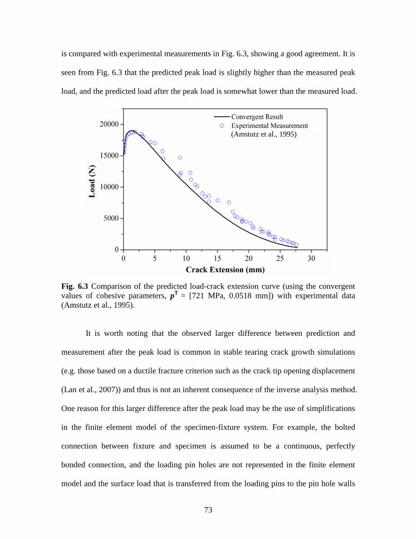
73
is compared with experimental measurements in Fig. 6.3, showing a good agreement. It is
seen from Fig. 6.3 that the predicted peak load is slightly higher than the measured peak
load, and the predicted load after the peak load is somewhat lower than the measured load.
Fig. 6.3 Comparison of the predicted load-crack extension curve (using the convergent
values of cohesive parameters, pT
= [721 MPa, 0.0518 mm]) with experimental data
(Amstutz et al., 1995).
It is worth noting that the observed larger difference between prediction and
measurement after the peak load is common in stable tearing crack growth simulations
(e.g. those based on a ductile fracture criterion such as the crack tip opening displacement
(Lan et al., 2007)) and thus is not an inherent consequence of the inverse analysis method.
One reason for this larger difference after the peak load may be the use of simplifications
in the finite element model of the specimen-fixture system. For example, the bolted
connection between fixture and specimen is assumed to be a continuous, perfectly
bonded connection, and the loading pin holes are not represented in the finite element
model and the surface load that is transferred from the loading pins to the pin hole walls
(Amstutz et al., 1995)

74
through bearing contact is simplified as a line of displacement loading at a line of finite
element nodes through the specimen thickness. Errors due to these simplifications will
tend to be larger at later stages of crack growth when the specimen-fixture system
experiences larger overall deformation and rotation. Another reason for this under-
estimation in both the CZM and CTOD based simulations, which is common in published
simulations (not just by the current authors), may be that these simulations assume
constant CZM parameter values or a constant critical CTOD value , while in reality these
values may be stress-state dependent. This issue is not pursued in this study because of
the relative insignificance of the later part of the load-crack extension curve.
Fig. 6.4 Variation of peak load with iterations.
To provide a quantitative understanding of the inverse iteration convergence trend,
Fig. 6.4 shows the variation of the predicted peak load of the load-crack extension curve
with the iteration number. It is seen that the predicted peak load goes towards the
(Amstutz et al., 1995)

75
measured value quickly in the first several iterations and then stays at a constant value,
then stops at a point with 1.5% difference of the measured value, thus demonstrating
iteration convergence. The convergence trend can also be observed by examining how
the value of the objective error function in Eq. (6.3) is reduced as iteration proceeds.
Fig. 6.5 Variation of the value of objective error function with iterations.
Figure 6.5 shows the variation of the objective error function with the iteration
number. It is clear from Fig. 6.5 that the value of the objective error function is quickly
reduced from a high value to a small constant value after 3 or 4 iterations (note that a
small error tolerance is placed on the corrections to the input parameter vector, not on the
objective error function itself).
6.4.2 Effect of Initial Values
In order to inspect the effect of the initial guess of the parameter vector in the
inverse analysis, two more sets of the initial values are employed and the inverse analyses
are carried out again. Referring with the manually obtained cohesive parameter values

76
(pT)m =[(Tmax)m, (δsep)m] = [759 MPa, 0.0448 mm](see Chapter 5), the new initial values
of the input vector are chosen without any preference in the feasible ranges (see Section
6.3) for two cases, namely [(Tmax)2 > (Tmax)m, (δsep)2 > (δsep)m] = [800 MPa, 0.058 mm]
and [(Tmax)3 > (Tmax)m, (δsep)3 < (δsep)m] = [900 MPa, 0.038 mm] (note that [(Tmax)1 <
(Tmax)m, (δsep)1 < (δsep)m] = [600 MPa, 0.04mm]).
Fig. 6.6 Variation of the values of objective error function with iterations for three
inverse analysis cases.
It is shown from Fig. 6.6 that, for all the three inverse analyses, the values of the
objective error function are quickly reduced from high values to a small constant. This
constant does not intend to zero due to the bigger difference between the predictions and
measurement at the later part of the load-crack extension curve. Particularly, it seems that
the inverse analysis case #3 needs more iterations at the earlier stage to seek the steepest
direction of the correction for the input vector and needs more iterations to converge,
since the two parameters are adjusted to the different directions.
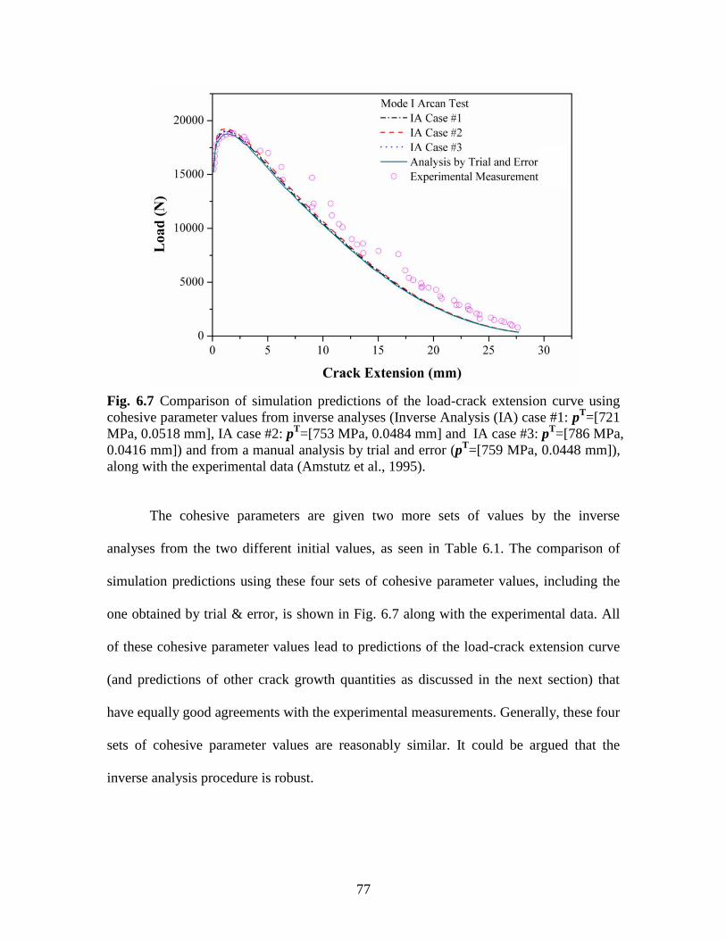
77
Fig. 6.7 Comparison of simulation predictions of the load-crack extension curve using
cohesive parameter values from inverse analyses (Inverse Analysis (IA) case #1: pT=[721
MPa, 0.0518 mm], IA case #2: pT=[753 MPa, 0.0484 mm] and IA case #3: p
T=[786 MPa,
0.0416 mm]) and from a manual analysis by trial and error (pT=[759 MPa, 0.0448 mm]),
along with the experimental data (Amstutz et al., 1995).
The cohesive parameters are given two more sets of values by the inverse
analyses from the two different initial values, as seen in Table 6.1. The comparison of
simulation predictions using these four sets of cohesive parameter values, including the
one obtained by trial & error, is shown in Fig. 6.7 along with the experimental data. All
of these cohesive parameter values lead to predictions of the load-crack extension curve
(and predictions of other crack growth quantities as discussed in the next section) that
have equally good agreements with the experimental measurements. Generally, these four
sets of cohesive parameter values are reasonably similar. It could be argued that the
inverse analysis procedure is robust.

78
Tab. 6.1 Comparison among the four distinct sets of cohesive parameter values obtained
from the inverse analyses and from analysis by trial and error.
Trial and Error IA#1 IA#2 IA#3
Initial Guess
pT= [Tmax , δsep]
[600MPa,
0.04mm]
[800MPa,
0.058mm]
[900MPa,
0.038mm]
Convergent Identification
pT= [Tmax , δsep]
[759MPa,
0.0448mm]
[721MPa,
0.0518mm]
[753MPa,
0.0484mm]
[786MPa,
0.0416mm]
Change of Tmax relative to
(Tmax)m 0 -5.00% -0.80% 3.60%
Change of δsep relative to (δsep)m 0 15.60% 8.00% -7.10%
Cohesive Energy, Π Tmaxδsep/2 17 MPa mm 18.67 MPa mm 18.22 MPa mm 16.35 MPa mm
Change of Π relative to Π m 0 9.80% 7.20% -3.80%
Predicted critical CTOD 0.078 mm 0.077 mm 0.079 mm 0.078 mm
6.4.3 (Non-)Uniqueness of Cohesive Parameters
However, one can still tell there are some differences among these sets of
obtained cohesive parameter values. Take an instance, the cohesive energy is considered
as an important parameter to define a cohesive law in practice. Some researchers claimed
that this parameter is a material property. The changes of cohesive energy relative to the
one used for finding the cohesive parameter values by trial & error are calculated and
shown in Table 6.1. The change varies from the range of -3.8% - 9.8%. This is consistent
with the observation in a previous study that the load-crack extension curve does depend
on the variation of Tmax when cohesive energy is kept constant. It is also noticed that for
all cases, the cohesive strength Tmax remains at around 2.2 σy. It is suggested that the
predicted load-crack extension curve is more sensitive to Tmax than to δsep.

79
In principle, the cohesive parameters are considered material properties associated
with stable tearing crack growth. They are expected to have unique values under the
given conditions. If the somewhat non-uniqueness of cohesive parameter values from the
current study is considered as an issue, then further investigation is needed. Implications
of the finding from this study are not clear at this time. The error function may have a flat
minimum, which leads to the small differences among the cohesive parameter values. Or
perhaps just the load-crack extension curve alone is not sufficient to determine a very
unique set of cohesive parameter values. In that case, what other crack growth quantities
must be considered to uniquely determine the cohesive parameter values?
In the literature, besides the load-crack extension curve that is most often chosen
for comparisons between predictions and measurements, the load-displacement curve
(displacement is the movement of the loading point on the fixture-specimen system) or
the displacement-crack extension curve is also used to analyze the structural integrity and
residual strength. However, the load-displacement curves or the displacement-crack
extension curves for the Arcan tests are not available from the experimental
measurements that are cited in the current study, because the slip in the fixture-machine
grip region that was held together by friction was sizable but could not be measured.
On the other side, the displacement-crack extension curves are predicted from the
current simulations using the four different sets of cohesive parameter values. As shown
in Fig. 6.8, this quantity is not sensitive to the variation of the cohesive parameter values,
although there are some differences among the curves. This observation demonstrates
that the displacement-crack extension curve will not ensure the uniqueness of the
cohesive parameter values either. Another question is, if the two cohesive parameters

80
cannot be identified from the inverse analysis simultaneously, is it possible to set up two
separate experiments that one is sensitive to Tmax and the other is sensitive to δsep? Further,
does it matter whether the cohesive parameter values are unique or not if they both
produce the same or similar predictions? These are open questions. The last question is
also related to another question: Does it matter whether one cohesive law or another is
used to simulate a given crack growth event if they both lead to the same or similar
predictions of relevant crack growth quantities?
Fig. 6.8 Comparison of the predictions of displacement-crack extension curve using the
four sets of cohesive parameter values obtained the inverse analyses.
6.4.4 Validations for Mixed-mode Cases and for CTOD Variations
Similar with Section 5.2, the cohesive parameters obtained from inverse analyses
using Mode I stable tearing crack growth tests will be validated by predicting mixed-
mode I/II loading cases. The details of finite element modeling in mixed I/ II cases can be
found in Section 5.2.

81
Fig. 6.9 Comparison of load-crack extension curves from experimental measurements
(Amstutz et al., 1995) and from CZM simulation predictions using cohesive parameter
values obtained from inverse analyses and obtained by trial & error for the 15° loading
case.
Fig. 6.10 Comparison of load-crack extension curves from experimental measurements
(Amstutz et al., 1995) and from CZM simulation predictions using cohesive parameter
values obtained from inverse analyses and obtained by trial & error for the 45° loading
case.
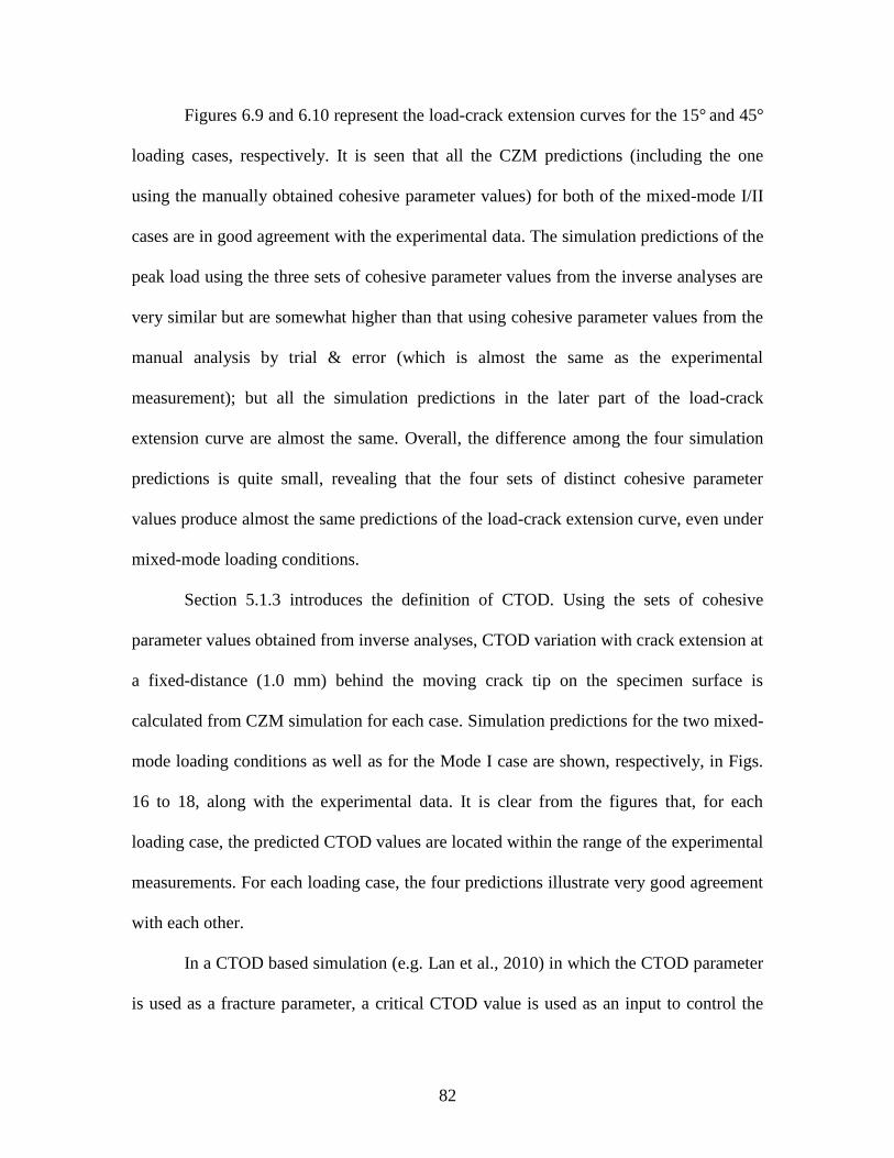
82
Figures 6.9 and 6.10 represent the load-crack extension curves for the 15° and 45°
loading cases, respectively. It is seen that all the CZM predictions (including the one
using the manually obtained cohesive parameter values) for both of the mixed-mode I/II
cases are in good agreement with the experimental data. The simulation predictions of the
peak load using the three sets of cohesive parameter values from the inverse analyses are
very similar but are somewhat higher than that using cohesive parameter values from the
manual analysis by trial & error (which is almost the same as the experimental
measurement); but all the simulation predictions in the later part of the load-crack
extension curve are almost the same. Overall, the difference among the four simulation
predictions is quite small, revealing that the four sets of distinct cohesive parameter
values produce almost the same predictions of the load-crack extension curve, even under
mixed-mode loading conditions.
Section 5.1.3 introduces the definition of CTOD. Using the sets of cohesive
parameter values obtained from inverse analyses, CTOD variation with crack extension at
a fixed-distance (1.0 mm) behind the moving crack tip on the specimen surface is
calculated from CZM simulation for each case. Simulation predictions for the two mixed-
mode loading conditions as well as for the Mode I case are shown, respectively, in Figs.
16 to 18, along with the experimental data. It is clear from the figures that, for each
loading case, the predicted CTOD values are located within the range of the experimental
measurements. For each loading case, the four predictions illustrate very good agreement
with each other.
In a CTOD based simulation (e.g. Lan et al., 2010) in which the CTOD parameter
is used as a fracture parameter, a critical CTOD value is used as an input to control the
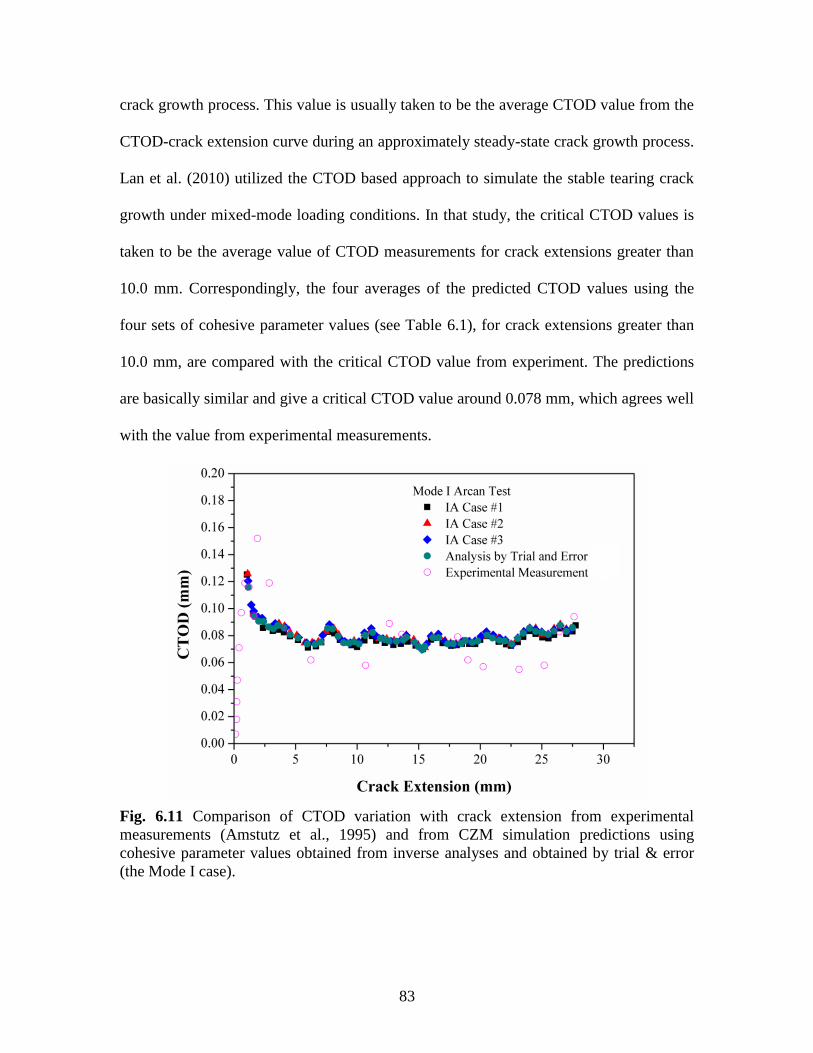
83
crack growth process. This value is usually taken to be the average CTOD value from the
CTOD-crack extension curve during an approximately steady-state crack growth process.
Lan et al. (2010) utilized the CTOD based approach to simulate the stable tearing crack
growth under mixed-mode loading conditions. In that study, the critical CTOD values is
taken to be the average value of CTOD measurements for crack extensions greater than
10.0 mm. Correspondingly, the four averages of the predicted CTOD values using the
four sets of cohesive parameter values (see Table 6.1), for crack extensions greater than
10.0 mm, are compared with the critical CTOD value from experiment. The predictions
are basically similar and give a critical CTOD value around 0.078 mm, which agrees well
with the value from experimental measurements.
Fig. 6.11 Comparison of CTOD variation with crack extension from experimental
measurements (Amstutz et al., 1995) and from CZM simulation predictions using
cohesive parameter values obtained from inverse analyses and obtained by trial & error
(the Mode I case).

84
Fig. 6.12 Comparison of CTOD variation with crack extension from experimental
measurements (Amstutz et al., 1995) and from CZM simulation predictions using
cohesive parameter values obtained from inverse analyses and obtained by trial & error
(the 15° loading case).
Fig. 6.13 Comparison of CTOD variation with crack extension from experimental
measurements (Amstutz et al., 1995) and from CZM simulation predictions using
cohesive parameter values obtained from inverse analyses and obtained by trial & error
(the 45° loading case).

85
6.5 Summary
The current Chapter has investigated the applicability of inverse analysis to the
identification of cohesive parameter values in cohesive zone model based simulations of
stable tearing crack growth in ductile materials. It is proposed that key points on the load-
crack extension curve can be used to create the error function in the inverse analysis. It is
found that a modified Levenberg-Marquardt method works well in identifying cohesive
parameter values with the feasible constraints. A Mode I stable tearing crack growth
experiment on a specimen made of 2024-T3 aluminum alloy is used for the inverse
analysis using the modified LM method. The inverse analysis proceeds in a very fast
convergence speed.
This study finds three sets of convergent solutions for cohesive parameter values,
by the inverse analyses, from three different sets of initial values. The differences among
the convergent solutions are small, which indicates the robust of the current inverse
procedure. With these sets of cohesive parameter values as well as the set obtained by
trial & error in Chapter 5, predictions of the load-crack extension curves for two mixed-
mode I/II cases and the variation of the critical CTOD with crack extension for both the
Mode I case and two mixed-mode I/II cases are validated with experimental data. In
addition, results from the current study attract further investigation to improve the
uniqueness of the cohesive parameter values associated with the simulation of stable
tearing crack growth.

86
CHAPTER 7
SIMULATIONS FOR MIXED-MODE I/III
STABLE TEARING CRACK GROWTH EVENTS
Thin sheets made of ductile materials e.g. aluminum alloys and steels are widely
used in load-bearing structures. In order to assess and predict lifetime of ductile thin-
sheet structure, it is necessary to understand the ductile fracture behaviors under certain
loading conditions. In practice, cracks in ductile thin-sheet structures are often subjected
to a combination of in-plane Mode I and Mode II and out-of-plane Mode III loading
conditions. While many investigations have been well carried out for Mode I fractures,
studies for mixed-mode cases, especially the ones involving a mode III component e.g.
mixed-mode I/III , are limited in the literature due to its complex nature.
Due to the complexity of crack-front stress and deformation fields under mixed-
mode I/III conditions, numerical simulations are almost always required to analyze or
predict ductile fracture events. Several approaches have been proposed for fracture
simulations, particularly for mixed mode I/III fracture of solids. In one approach, crack
growth is controlled by a proper crack growth criterion e.g. a short summary see in Liu
et al., 4 .
Chapter 4 to 6 developed a 3D FE model to simulate both Mode I and mixed-
mode I/II stable tearing crack growth events in Arcan specimens made of 4-T3
87
aluminum alloy based on the CZM approach. The load-crack extension curves and
critical CTOD variation with crack extensions were predicted and very well validated by
experimental measurements. The results also show a strong connection between the CZM
approach and the CTOD based approach for simulation of stable tearing crack growth
events. In this chapter, the study is aimed at investigating the applicability of the CZM
approach in simulating mixed-mode I/III stable tearing crack growth events in ductile
materials under large deformation. In the investigation, the triangular cohesive law will
be employed in the CZM approach to simulate the stable tearing crack growth events in
the specimens made of 6061-T6 aluminum alloy and GM6028 steel under combined in-
plane and out-of-plane loading conditions (Sutton et al., 2007; Yan et al., 2009) (see
Section 2.2). The fracture events in laboratory specimens contain uncertainties in the
specimen-fixture connection region and as such modeling of the entire specimen -
loading fixture system seems not advisable. To avoid these uncertainties, a hybrid
modeling approach developed in (Wei et al., 2011) will be employed in the current study.
A specimen region away from the specimen-fixture connections but engulfing the
complete crack growth process is modeled. Time dependent boundary conditions for the
modeling region are derived from full-field surface displacement measurements.
Simulation predictions of time history of crack extension and the CTOD variation with
crack extension will be compared with experimental measurements as well as with the
predictions from a CTOD simulation.
7.1 Sub-Region Model
In the experiment, the specimen and fixture were connected through compression
and friction. The potential slippage between the fixture and specimen and the severe

88
specimen stretching around the grips introduce complications and uncertainties in the
connection region, which are hard to model and quantify in the simulations. Thus,
although modeling the entire specimen-fixture system and applying the boundary
conditions on the real positions is direct and convenient, it is difficult to employ this
approach for our particular problem in finite element analysis. In order to avoid such
complications and uncertainties in the specimen-fixture connection region, Wei et al.
(2011) proposed a sub-region modeling approach for the study of the mixed-mode I/III
stable tearing crack growth using CTOD based simulation approach. In this approach, the
finite element model considers only a sub-region of the specimen, where is away from
the specimen-fixture connections but contains complete crack growth process. Images of
the randomly patterned specimen surface were recorded by the stereo-vision system
during the experiments. Although the sub-region is not limited to a particular shape, a
simple rectangular shape is taken for simplicity.
For an instance of the case of mixed-mode I/III specimen loaded at an angle of Ф
= 60°, the sub-region of the specimen is shown in Fig. 7.1. The in-plane geometry is the
area enclosed by the outline ABCDEF. This sub-region is “cut out” from the whole
specimen with planes perpendicular to the area ABCDEF along edge AB, BC, CD, DE
and EF. In Fig. 7.1, the modeled region is located below the specimen-fixture
connections. In the area above the modeled region, the right portion of the specimen is
connected to the fixed grip while the left portion is attached to the moving grip. Fig. 7.1
also shows the coordinate system employed in experiments and finite element analyses,
with the origin of the coordinate system being located at the tip of the pre-crack. The
initial crack orientation is aligned with the X axis direction. The displacement
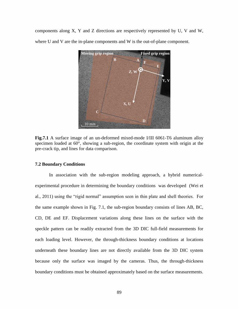
89
components along X, Y and Z directions are respectively represented by U, V and W,
where U and V are the in-plane components and W is the out-of-plane component.
Fig.7.1 A surface image of an un-deformed mixed-mode I/III 6061-T6 aluminum alloy
specimen loaded at 60°, showing a sub-region, the coordinate system with origin at the
pre-crack tip, and lines for data comparison.
7.2 Boundary Conditions
In association with the sub-region modeling approach, a hybrid numerical-
experimental procedure in determining the boundary conditions was developed (Wei et
al., 2011) using the “rigid normal” assumption seen in thin plate and shell theories. For
the same example shown in Fig. 7.1, the sub-region boundary consists of lines AB, BC,
CD, DE and EF. Displacement variations along these lines on the surface with the
speckle pattern can be readily extracted from the 3D DIC full-field measurements for
each loading level. However, the through-thickness boundary conditions at locations
underneath these boundary lines are not directly available from the 3D DIC system
because only the surface was imaged by the cameras. Thus, the through-thickness
boundary conditions must be obtained approximately based on the surface measurements.
A B
D
E
C
F
Moving grip region Fixed grip region
X, U
Z, W
Y, V
10 mm

90
Specifically, the normal of the specimen’s upper surface is assumed to be rigid and
remain perpendicular to the upper surface during the deformation process. This
assumption is reasonable since the thickness of the specimen is less than 1/10 of the in-
plane dimension of the specimen so that the sub-region can be regarded as a thin plate.
Using the “rigid normal” assumption, boundary displacements at any point
through the thickness of the sub-region boundary lines can be extrapolated from the
displacement measurements on the upper surface, as illustrated schematically in Fig.7.2.
The Z axis is along the thickness direction of the specimen. The boundary surface BCHG
is a cutting side perpendicular to the front surface BCDE in the un-deformed
configuration. Suppose P0 is a point on the boundary line BC and P is a point on the
boundary surface BCHG such that PP0 is the through-thickness line aligned with the
normal of the upper surface at P0 (which is parallel to the Z axis) in the un-deformed
configuration. When the specimen is deformed, the upper surface BCDE may become a
curved surface (see Fig. 7.2 (b)). Let vector N be the normal vector of the deformed
upper surface at point P0. Based on the rigid normal assumption, the line PP0 in the
deformed configuration is still aligned with the normal vector N, and the distance |PP0|
from P to P0 remains unchanged. Mathematically, if the displacements at P0 and the
orientation of N are known, then the displacements at point P at a distance of |PP0| away
from P0 can be readily determined.
Since the 3D DIC measurement system employed in the mixed-mode I/III stable
tearing experiments provides both the deformed and un-deformed position for each point
throughout the loading process, the orientation of the normal vector at each point on the
deformed surface is determined as follows. For the point P0 on the boundary line BC in

91
the un-deformed configuration (see Fig. 7.2 (a)), choose a supplementary line B1C1
parallel to and near BC (say, at a distance of 0.5 mm away, which is used in this study).
In the deformed configuration, the tangent vector T of the deformed curve BC at point P0
is calculated, and an in-plane vector S is created from P0 to an adjacent point on the
deformed line B1C1. Then the normal vector N of the deformed upper surface at point P0
can be determined by using the direction of the cross product of vectors S and T. In order
to reduce the noise of displacement measurements from the 3D DIC system, a local
smoothing algorithm is always employed when interpolate the displacement values for a
given location along each boundary line (e.g., BC) or complementary line (e.g., B1C1) in
the current study, such that all neighboring experimental data points within a certain
distance from the given location are fitted into a 3rd
order polynomial. Using this method,
the boundary conditions are determined at any point on the through-thickness surfaces
underneath the boundary lines on the upper surface according to the mesh in finite
element analysis.
(a) (b)
Fig.7.2 A schematic showing a sub-region in (a) an un-deformed configuration and (b) a
deformed configuration.
P0
C
B C1
S
B1
N
T
Z
P
G
D
E
H
B
C1
P0 P
B1
Z
E D
G H
C
Front surface
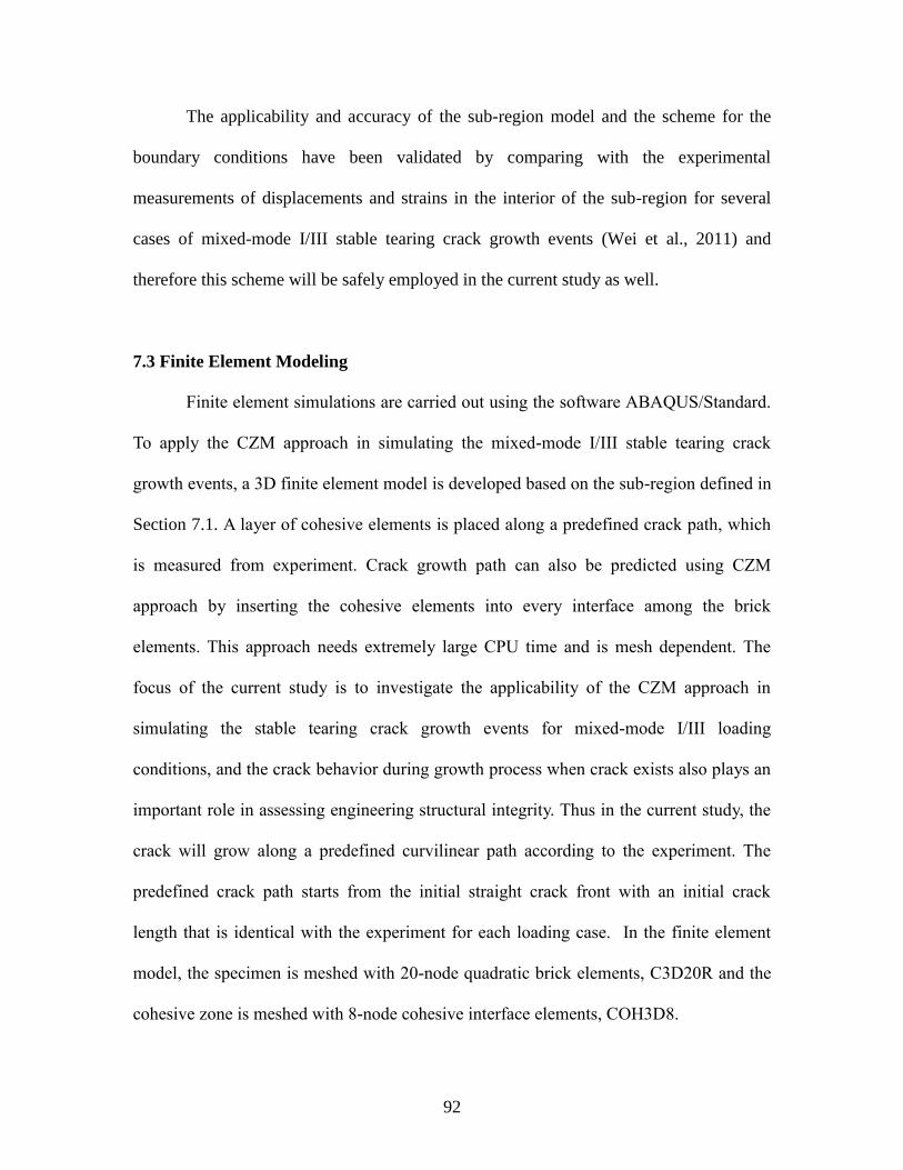
92
The applicability and accuracy of the sub-region model and the scheme for the
boundary conditions have been validated by comparing with the experimental
measurements of displacements and strains in the interior of the sub-region for several
cases of mixed-mode I/III stable tearing crack growth events (Wei et al., 2011) and
therefore this scheme will be safely employed in the current study as well.
7.3 Finite Element Modeling
Finite element simulations are carried out using the software ABAQUS/Standard.
To apply the CZM approach in simulating the mixed-mode I/III stable tearing crack
growth events, a 3D finite element model is developed based on the sub-region defined in
Section 7.1. A layer of cohesive elements is placed along a predefined crack path, which
is measured from experiment. Crack growth path can also be predicted using CZM
approach by inserting the cohesive elements into every interface among the brick
elements. This approach needs extremely large CPU time and is mesh dependent. The
focus of the current study is to investigate the applicability of the CZM approach in
simulating the stable tearing crack growth events for mixed-mode I/III loading
conditions, and the crack behavior during growth process when crack exists also plays an
important role in assessing engineering structural integrity. Thus in the current study, the
crack will grow along a predefined curvilinear path according to the experiment. The
predefined crack path starts from the initial straight crack front with an initial crack
length that is identical with the experiment for each loading case. In the finite element
model, the specimen is meshed with -node quadratic brick elements, C3D R and the
cohesive zone is meshed with 8-node cohesive interface elements, COH3D8.

93
(a) (b)
Fig. 7.3 (a) A 3D mesh for aluminum alloy 6061-T6 specimen under the 60° mixed-mode
I/III loading case; (b) A zoom-in view showing the cohesive zone along the crack path.
To gain confidence in the accuracy of simulation predictions, convergence study
of the finite element mesh density is carried out carefully before major simulations. Fig.
7.3 a shows an overall view of a final refined mesh of the sub-region of aluminum
specimen for 6 ° mixed-mode I/III loading. The brick element size is about .5 mm.
Similarly, a convergence study is performed on the cohesive element size h when the
mesh elsewhere is already converged. It is found that a cohesive element size of h . 5
mm is sufficient for convergence and 16 layers of cohesive elements are needed through
the thickness of the specimen. A zoomed in view of the cohesive zone mesh can be found
in Fig. 7.3 b . Displacement boundary conditions for the sub-region boundary were
generated using continuous 3D DIC measurements based on the scheme described in the
Section 7.2. Since the images are taken at very small time increment (i.e., very small load

94
increment during the experiment, there are enough discrete “snap shots” of the whole
deformation history of the specimen. Therefore, the sub-region model with boundary
conditions generated from those discrete images will well approximate the continuous
deformation process of the real specimen.
Several studies (e.g. Kamat et al., 1995; Liu et al., 2004) reported that with the
Mode III loading increasing, fracture criterion, e.g. fracture toughness or fracture strength,
of ductile materials reduces comparing with Mode I case. However, there has not been a
well-established rule regarding the effect of mode mixity on the selections of cohesive
parameters for mixed-mode ductile crack growth in the literature. In the current study, the
cohesive strengths Tmaxi are assumed to be the same as Tmax for all mode I, II and III
directions because of the isotropic property of metallic material. In addition, in the
reference by Zavattieri 6 , two factors 1 and 2 were introduced to describe the
effects of two shear components in defining a triangular cohesive law. In the simulations,
these two factors were assumed as 1.0, which means the cohesive parameters for normal
and two shear directions were assumed to be the same. Therefore, following this
simplification, we also assume the cohesive parameters are same for the three directions.
The initial cohesive stiffness K is assigned as a large value, which is larger than
100 E/L (E is the stiffness of the specimen and L is the overall dimension of the
specimen), so that the overall structural stiffness or compliance of the specimen is not
affected. The other two cohesive parameters, Tmax and δsep, are chosen as the input
parameters in the simulations. The details of selections of these two parameters will be
discussed in the next section.

95
7.4. Results and Discussions
7.4.1 Calibration of CZM Parameters
In Chapter 5 and 6, two ways of selecting cohesive parameter values for ductile
materials, such as 2024-T3 aluminum alloy, in simulating Mode I and mixed-mode I/II
loading stable tearing crack growth events were discussed, which are (1) by both trials &
error and (2) by inverse approaches. Similarly, for each material in the current Chapter,
6061-T6 aluminum alloy and GM6208 steel, the cohesive parameters Tmax and δsep will be
estimated by trial & error through matching predictions of crack extension time history
curve with the experimental measurements for 30° mixed-mode I/III loading condition.
Then the obtained cohesive parameters will be validated with the experiment by
predicting other fracture quantities. It is noted that, in the literature, the load-crack
extension curve and load-displacement curve (displacement is the movement of the
loading point on the fixture-specimen system) are often chosen for comparisons between
predictions and measurements to analyze the structural integrity and residual strength.
However, the load-crack extension curve or load-displacement curve for Mixed-mode
I/III tests is not available from the experimental measurements that are cited in the
current study, because the slip in the fixture-machine grip region that was held together
by friction was sizable but could not be measured. On the other side, since a sub-region
model that does not contain the loading boundary is used in the finite element analysis,
the external loading applied on the entire test is impossible to be calculated from the sub-
region model. Therefore, the crack extension-time curve is used as the measurements to
be compared with simulation predictions for determining and validating CZM parameters
for the two materials.

96
In practice, some reference values or feasible ranges of values are usually sought
in order to reach efficient and reasonable solutions of the input cohesive parameters in
simulations. The cohesive energy is generally accepted to be equal to the facture energy
of the material. Some researchers claim that this parameter is a material property. Thus
the cohesive energy is usually selected as a reference constant or an input parameter to
define cohesive law. For example, the cohesive energy in (Li and Siegmund, 2002) is
taken to be 17 KJ/m2 for simulating crack growth in thin sheet 2024-T3 aluminum alloy.
However, this reference is hard to be applied to our particular problem, because: (a)
Mode III fracture energies for the two materials in the current study have not been
reported in the literature; (b) Due to the complexity of mode mixity, mixed-mode fracture
energy cannot be calculated by simply combining the component values of individual
modes; (c) The results in Section 5.1.1 show that, when cohesive energy is kept constant,
the prediction does depend on the selection of Tmax and δsep. Therefore, in the current
study, Tmax and δsep will be selected without any reference on the fracture energies for the
materials.
In the literature, the value of the cohesive strength Tmax for various cohesive laws
has been estimated mostly based on the initial yield stress σy of the material surrounding
the cohesive zone. In the reference, Li and Siegmund (2002) summarized that the ratio
Tmax/σy ranges from 1.2 to 4 for different conditions and they chose 2σy as the cohesive
strength in their models. The results from Chapter 5 and 6 showed that when Tmax is
around 2.2 σy, predictions agree with the experimental measurements well. Therefore, in
the current study, the cohesive strength Tmax is chosen from the range of 1.0σy to 4.0σy.

97
Following the considerations above, a series of simulations of 30° mixed-mode
I/III stable tearing crack growth have been carried out using various cohesive parameter
values for 6061-T6 aluminum alloy and GM 6028 steel respectively. Simulation
predictions of crack extension-time curve are compared with experimental measurements.
After a range of trials, a proper set of CZM parameter values is found for each material.
Fig. 7.4 and Fig. 7.5, respectively, show the comparison of the predictions and
measurements for 6061-T6 aluminum alloy and GM 6028 steel under 30° loading. For
both cases, the predicted crack extension-time histories agree reasonably well with the
experimental measurements. Overall, the predicted crack growths are slightly faster than
the measured curves.
It is noticed that, however, the predicted crack growth are much faster than the
measured ones at the early stage, especially in the case of GM 6028 steel in which the
difference between prediction and measurements is more noticeable. One plausible
reason for this predicted faster crack initiation speed is that the simulation assumes
constant CZM parameter values during the crack growth, while in reality these values
may be stress-state dependent. To better understand this issue, the predictions from a
CTOD based simulations are compared with the current predictions and with
experimental measurements for each material respectively.
It has been observed in the experimental investigations that, during the crack
extension, the critical CTOD has always a higher initial value and then maintains at a
constant average (e.g. Fig. 7.6). This constant average is usually used in numerical
studies as the criterion to control the crack growth process from initiation to failure (e.g.
Newman, 1984; Gullerud et al, 1999; Deng and Newman, 1999). However, observing

98
from the experiments of mixed-mode I/III stable tearing crack growth, materials around
the initial crack front experienced extremely large deformation from the un-deformed
state to a critical state. A constant criterion may not be able to capture the whole crack
growth procedure. As seen in Fig. 7.4 and Fig. 7.5, the initial higher portion of CTOD
accounts for the discrepancy of the predicted (using a constant criterion) (Wei, 2008;
2011) and measured crack extension-time histories especially in the early stage of crack
extension. As such, further simulations were performed in (Wei, 2008; 2011) using a
bilinear CTOD criterion (see Fig. 7.6) instead of a constant average value. As shown in
Fig. 7.4 and Fig. 7.5, using these bilinear CTOD criteria, the accuracy of the predicted
crack extension time history are improved for both materials (especially for GM 6028
steel, the improvement is obvious).
Fig. 7.4 For 30° mixed-mode I/III loading condition in 6061-T6 aluminum alloy, the
predicted crack extension history curve using CZM simulation (Tmax =763.6 MPa, δsep =
0.02 mm) agrees with the experimental measurement (Sutton et al., 2007; Yan et al.,
2009) and with predictions from CTOD simulations (Wei, 2008; 2011).

99
Fig. 7.5 For 30° mixed-mode I/III loading condition in GM 6028 steel, the predicted
crack extension history curve using CZM simulation (Tmax =1288.2 MPa, δsep = 0.04mm)
agrees with the experimental measurement (Sutton et al., 2007; Yan et al., 2009) and with
predictions from CTOD simulations (Wei, 2008; 2011).
For 30° mixed-mode I/III loading in 6061-T6 aluminum alloy (Fig. 7.4), the CZM
prediction is similar with the bilinear CTOD simulation prediction and slightly closer to
the measurement than the constant CTOD simulation. All the three predictions agree well
with the measurement. On the other hand, for the case of 30° mixed-mode I/III loading in
GM6028 steel (Fig. 7.5), the CZM predicted crack extension time history is closer to the
measurement than the constant CTOD simulation but the agreement with measurements
is not as good as the prediction using a bilinear CTOD. Similar to the effects of a constant
CTOD versus a bilinear CTOD in CTOD based simulation, the prediction of an earlier
crack growth initiation was reasonably expected in the simulation when constant CZM
parameters were used as a criterion to control crack growth throughout the history of
crack extension. In addition, comparing with the aluminum alloy, the initial critical
CTOD value for the steel case is very high and the lower constant critical CTOD value

100
comes much later, as shown in Fig. 7.6. This is why the assumption of constant CZM
parameters has a stronger effect in steel simulations than in aluminum simulations.
(a)
(b)
Fig. 7.6 Bilinear fitting of the measured CTOD versus crack extension for the quasi-static,
mixed-mode I/III 6061-T6 aluminum alloy and GM6208 specimens at different loading
angle Ф: a 6061-T6 aluminum alloy, Ф 3 °; b 6061-T6 aluminum alloy, Ф 6 °; c
GM6208, Ф 3 °; d GM6 8, Ф 6 °. The bilinear curve was used in the simulation to
control the crack extension (Wei, 2008; 2011).

101
7.4.2 Validation with Experiment
7.4.2.1 Crack Extension-Time Curve for 60° Mixed-mode Loading
CZM simulations of stable tearing crack growth for 60° mixed-mode I/III loading
condition are performed again in aluminum and steel specimens respectively. The sub-
region FE modeling approach described above and the results of convergence study on
meshes are carried through to the 60° cases. Using the same sets of cohesive parameter
values from 30° simulations, the predicted crack extension-time curves are presented and
compared with experimental data and with two CTOD based (constant and bilinear
criterion) simulation predictions in Fig. 7.7 and Fig. 7.8 for the two materials respectively.
Correspondingly with the 30° cases, CZM predictions are similar with the two
CTOD based simulation predictions (Wei, 2008) in 6061-T6 aluminum alloy specimen,
showing very good agreement with the experimental measurement. In contrast, for GM
6028 steel, the CZM simulation prediction of crack extension is slightly faster than the
experimental data, while the bilinear CTOD prediction is slightly slower than the
experiment. At the early crack growth stage, the CZM prediction is closer to the
measurement than the constant CTOD simulation but the agreement with measurements
is not as good as the prediction using a bilinear CTOD. The difference of the simulations
in the two materials shows that the effect of stress state during the crack growth is server
in steel than that in aluminum alloy, which is same with the observations in 30° cases.
Although the CZM simulation predictions cannot perfectly match the
experimental measurements, the predictions have the same trend and, overall, agree
reasonably well with the experiment. For both materials, the CZM parameters obtained
from the 30° loading simulations are well validated by the 60° loading experiments.

102
Fig. 7.7 For 60° mixed-mode I/III loading condition in 6061-T6 aluminum alloy, the
predicted crack extension history curve using CZM simulation (Tmax =763.6 MPa, δsep =
0.02mm) agrees with the experimental measurement (Sutton et al., 2007; Yan et al., 2009)
and with predictions from CTOD simulations (Wei, 2008; 2011).
Fig. 7.8 For 60° mixed-mode I/III loading condition in GM 6028 steel, the predicted
crack extension history curve using CZM simulation (Tmax =1288.2 MPa, δsep = 0.04mm)
agrees with the experimental measurement (Sutton et al., 2007; Yan et al., 2009) and with
predictions from CTOD simulations (Wei, 2008; 2011).

103
7.4.2.2 CTOD Variation with Crack Extension
In Chapter 5 and 6 for the simulations of mixed-mode I/II stable tearing crack
growth events, it is found that the critical CTOD value used in CTOD based simulations
can be predicted using the CZM approach. The fact that CZM and CTOD based
simulation predictions agree with each other and with experimental data and that the
critical CTOD value can be predicted by CZM based simulations establish an equivalence
between the CZM and CTOD based approaches. In order to examine whether this
equivalence holds for general mixed mode stable tearing crack growth and to further
validate the CZM simulation and the obtained cohesive parameters for mixed-mode I/III
cases, the variation of CTOD with crack extension is calculated, for 6061-T6 aluminum
alloy and GM 6028 steel respectively, at a distance of 1.0mm behind crack tip from CZM
simulations for both 30° and 60° mixed mode loading conditions.
The CZM simulation predictions of CTOD variations are shown in Figs. 7.9 and
7.10 for 6061-T6 aluminum alloy and GM 6028 steel, respectively, along with the
experimental data. It is seen from the figures that, for each material, the predicted and
measured CTOD variations are in good agreement with each other and that the CTOD
value is higher initially and then stabilizes to constant mean value after an initial stage of
crack extension for both mixed-mode I/III loading conditions.
In a CTOD based simulation, the critical CTOD value used as an input to control
the crack growth process is usually taken to be the average CTOD value from the CTOD-
crack extension curve during an approximately steady-state crack growth process. In the
constant CTOD based simulation by Wei et al. 11 , the critical CTOD value is taken to
be the average value of CTOD measurement for crack extension greater than . mm for

104
the aluminum and 4. mm for the steel respectively. Using the same method, the averages
for the two materials are calculated from the simulations and compared with the
experimental averages in Figs. 7.9 and 7.1 . Fig. 7.9 shows that for 6 61-T6 aluminum
alloy specimen the predicted CTOD average agrees well with the measured one, which is
around .4 mm. But for GM 6 8 steel, as shown in Fig. 7.1 , the predicted CTOD
average, which is about .71 mm, is a little higher than the measurement that is .65 mm.
The effect of initial crack extension is considered as a plausible reason for this difference.
In addition, if more trials of the input cohesive parameters are performed, better
agreement may be reached.
Fig. 7.9 Comparison of predicted and measured CTOD variation with crack extension for
30° and 60° mixed-mode I/III loading conditions in 6061-T6 aluminum alloy specimens.
The average CTOD value for crack extensions greater than 2.0 mm beyond which the
CTOD variation oscillates around the average value for experiment (0.395 mm (Sutton et
al., 2007; Yan et al., 2009)) and prediction are the same.
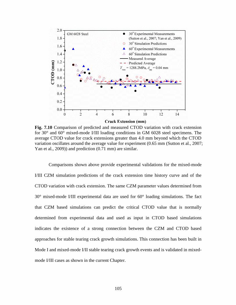
105
Fig. 7.10 Comparison of predicted and measured CTOD variation with crack extension
for 30° and 60° mixed-mode I/III loading conditions in GM 6028 steel specimens. The
average CTOD value for crack extensions greater than 4.0 mm beyond which the CTOD
variation oscillates around the average value for experiment (0.65 mm (Sutton et al., 2007;
Yan et al., 2009)) and prediction (0.71 mm) are similar.
Comparisons shown above provide experimental validations for the mixed-mode
I/III CZM simulation predictions of the crack extension time history curve and of the
CTOD variation with crack extension. The same CZM parameter values determined from
30° mixed-mode I/III experimental data are used for 60° loading simulations. The fact
that CZM based simulations can predict the critical CTOD value that is normally
determined from experimental data and used as input in CTOD based simulations
indicates the existence of a strong connection between the CZM and CTOD based
approaches for stable tearing crack growth simulations. This connection has been built in
Mode I and mixed-mode I/II stable tearing crack growth events and is validated in mixed-
mode I/III cases as shown in the current Chapter.

106
7.4.3 (Non-) Uniqueness of CZM Parameter Values
During the course of this study, an interesting issue was noticed that multiple sets
of CZM parameter values can be found, that lead to similar simulation predictions and
acceptable agreement with the experimental measurements. For example, using three
more different sets of cohesive parameters values, CZM simulation predictions in 6061-
T6 aluminum alloy under two mixed-mode I/III loadings are compared with the
experimental data of both the crack extension history curve (Fig. 7.11 a, c, e) and the
CTOD variation with crack extension (Fig. 7.11 b, d, f). The three predictions of crack
extension-time curve are very similar, showing very good agreement with the
experimental measurement. The predicted CTOD variations with crack extension are
more or less higher than the measured ones. Bigger difference is shown in Fig. 7.11 d,
because the predicted initial higher CTOD duration is longer than what is seen in the
experiment. The measured CTOD value stabilizes at a constant after the crack extends 2
mm, while the prediction delays this point to about 4 mm. But overall, all the three sets of
CZM parameters as well as the first one mentioned in the last section give very good
predictions. Particularly, when Tmax =763.6 MPa, δsep = 0.02mm (Fig. 7.4, 7.7, 7.9), Tmax
= 664MPa, δsep = 0.03mm (Fig. 7.11 a, b) and Tmax = 431.6 MPa, δsep = 0.07mm (Fig.
7.11 e, f), the predictions are almost the same. In these “proper” sets of cohesive
parameters, Tmax and δsep has a negative linear relationship. It is also inferred that more
sets of such cohesive parameters which may reach good predictions can be found but will
not be shown here. Among the results in the current study, the cohesive strength Tmax of
6061-T6 aluminum alloy varies from 1.3 σy to 2.3 σy.

107
The same issue happens in the CZM simulations of mixed-mode I/III crack
growths in GM 6028 steel specimen. Multiple sets of cohesive parameters have been
reached to lead to the similar predictions and to match the experimental measurements, as
shown in Fig. 7.12. Although the predictions for the steel are not as good as the ones for
the aluminum alloy due to the possible reason of stress state dependence, the trend of
predictions is the same as the experiment and the agreement between the predictions and
the measurements is acceptable. The cohesive strength Tmax of GM 6028 steel presented
in the current study is in the range of 2.5 σy to 4 σy. The ratio Tmax/ σy of the steel is higher
than that for the aluminum alloy.
In principle, the cohesive parameters are considered as material properties
associated with stable tearing crack growth. They are expected to have unique values
under the given conditions. The non-uniqueness of cohesive parameter values has been
observed in a previous study, in which multiple sets of cohesive parameters were
obtained from the inverse analysis in simulating mixed-mode I/II stable tearing crack
growth events (see Chapter 6). Comparing with the large ranges of cohesive parameter
values for the current materials, the variation range of the cohesive parameter values of
2024-T3 aluminum alloy for mixed-mode I/II cases is relative small. To understand the
implications of the non-uniqueness, several considerations were discussed in Chapter 6.
The results indicated that: (a) The calculated cohesive energy from the cases with good
predictions does not tend to a same value; (a large variation ranges of calculated cohesive
energy is found in the mixed-mode I/III cases, which is consistent with this previous
observation) (b) Multiple sets of cohesive parameters can lead to similar or same
predictions of the load-crack extension curve, the load-displacement (or displacement-
108
crack extension) curve and CTOD variation with crack extension, which are important
fracture quantities in assessing engineering structures. Neither these quantities nor the
crack extension-time curve used in the current chapter will ensure the uniqueness of the
cohesive parameters in simulating ductile crack growth events.
One possible reason for this non-uniqueness phenomenon is that the bulk
materials (aluminum and steel) are treated as elastic-plastic following the J2 flow theory
of plasticity. When material approaches to large plastic deformation, stress increases
slightly with large strain increment and the strict one-to-one stress-strain relationship
becomes vague. Consequently, the unique cohesive traction-separation relationship is
hard to be established. The stable tearing crack growth events, especially the mixed-mode
I/III cases, involve extremely large plastic deformation. Then, multiple cohesive
parameters give similar predictions becomes expected. This also explains why the
variation ranges of the cohesive parameters that lead to good predictions in mixed-mode
I/III simulations are larger than the ones in mixed-mode I/II cases. The plastic
deformation of specimen under mixed-mode I/III loading is much larger than that under
mixed-mode I/II loading.
Another consideration is the stress state around the crack tip, which is not
examined in the current study. Cohesive parameters may depend on the stress state
around the crack tip and thus may vary with crack extension. The relationship of cohesive
parameters and stress distribution may give stricter constraints on the selection of
cohesive parameters in simulations. For example, in this study, the selection range of Tmax
is from 1.0 σy to 4.0 σy of the bulk materials. This range may be too large, so that some of
the “proper” sets of cohesive parameters are not reasonable for the real physical problem.

109
(a) (b)
(c) (d)
(e) (f)
Fig. 7.11 Different sets of cohesive parameter values lead to similar predictions of crack
extension history curve (a, c, e) and CTOD variation with crack extension (b, d, f), all of
which agree reasonably with the experimental measurements for both 30° and 60° mixed-
mode I/III loading conditions in 6061-T6 aluminum alloy specimens. (a, b: Tmax =
664MPa, δsep = 0.03mm; c, d: Tmax = 498 MPa, δsep = 0.06mm; e, f: Tmax =431.6 MPa, δsep
= 0.07mm.)

110
(a) (b)
(c) (d)
(e) (f)
Fig. 7.12 Different sets of cohesive parameter values lead to similar predictions of crack
extension history curve (a, c, e) and CTOD variation with crack extension (b, d, f), all of
which agree reasonably with the experimental measurements for both 30° and 60° mixed-
mode I/III loading conditions in GM 6028 steel specimens. (a, b: Tmax = 1356 MPa, δsep =
0.03 mm; c, d: Tmax = 1186.5 MPa, δsep = 0.05mm; e, f: Tmax = 847.5 MPa, δsep = 0.1mm.)

111
More open questions are proposed, such as: If the two cohesive parameters cannot
be identified from the fracture quantities above simultaneously, is it possible to set up
two separate experiments that one is sensitive to Tmax and the other is sensitive to δsep?
Further, does it matter whether the cohesive parameter values are unique or not if they
both produce the same or similar predictions? Does it matter whether one cohesive law or
another is used to simulate a given crack growth event if they both lead to the same or
similar predictions of relevant crack growth quantities? All of these questions require
further investigations.
7.5 Summary
A cohesive zone model (CZM) approach has been applied to simulate mixed-
mode I/III stable tearing crack growth events in the specimens made of 6061-T6
aluminum alloy and GM 6028 steel. 3D finite element models based on a sub-region
modeling approach are developed in ABAQUS employing the triangular CZM law. For
each material, CZM parameter values are determined through matching simulation
predictions of the crack extension-time curve with experimental measurements for 30°
mixed-mode I/III loading. As experimental validations, the CZM simulation predictions
of the crack extension-time curve and of the CTOD variations with crack extension for
two mixed-mode cases (30° and 60° loading conditions) are shown to agree well with
experimental measurements.
Results from this Chapter show the applicability of CZM approach in simulating
mixed-mode I/III stable tearing crack growth events. But the assumption of constant
cohesive parameter values may not capture the whole crack growth process due to the

112
possible stress-state dependence. Initial larger values need to be taken account, especially
for the steel which has a higher stiffness. It is found that both CZM and CTOD
approaches produce very similar simulation predictions of the crack extension-time curve
and that the critical CTOD value used in CTOD based simulations, which is
conventionally determined from experimental data, can be predicted using the CZM
based approach. This fact reaffirmed an equivalence between the CZM and CTOD based
simulation approaches, which has been established from a previous study of mixed-mode
I/II stable tearing crack growth events in ductile materials. In addition, multiple sets of
CZM parameters are found, which provide very similar predictions in simulating mixed-
mode I/III stable tearing crack growths. The uniqueness of cohesive parameters
associated with the simulation of stable tearing crack growth requires further
investigations.

113
CHAPTER 8
CONCLUSIONS AND FUTURE WORK
A cohesive zone model (CZM) based approach has been successfully applied to
simulate Mode I, mixed-mode I/II and mixed-mode I/III stable tearing crack growth
events in ductile materials (e.g. aluminum alloy and steel). 3D finite element models are
developed in ABAQUS employing a triangular CZM law.
The simulations of Mode I and mixed-mode I/II stable tearing crack growths are
based on Arcan tests in 2024-T3 aluminum alloy. A proper set of CZM parameter values
is determined through matching simulation predictions of the load-crack extension curve
with experimental measurements for the Mode I case. The effects of CZM parameters
Tmax and δsep on the load-crack extension curve are discussed. As experimental
validations, the CZM simulation predictions of the load-crack extension curve for two
mixed-mode cases and of the CTOD variation with crack extension for the mixed-mode
as well as Mode I case are shown to agree well with experimental measurements.
The current results show that there is a strong connection between the CZM based
approach and the CTOD based approach for simulations of stable tearing crack growth
events. It is found that both approaches produce almost the same simulation predictions
of the load-crack extension curve. It is also found that the critical CTOD value used in
CTOD based simulations, which is conventionally determined from experimental data,

114
can be predicted using the CZM based approach. The fact that CZM and CTOD based
simulation predictions of the load-crack extension curve agree with each other and with
experimental data and that the critical CTOD value used in CTOD based simulations can
be predicted by CZM based simulations establish certain equivalence between the CZM
and CTOD based simulation approaches.
A helpful experience from the current study is that simulations of stable tearing
crack growth events using the CZM approach require careful convergence studies, not
just with respect to the standard finite element discretization, but also with respect to the
cohesive element length relative to the cohesive zone size and with respect to the values
of artificial parameters employed in implicit and explicit solution schemes.
In order to identify the values of the cohesive parameters in an automatic and
systematic manner, a modified Levenberg-Marquardt method based inverse analysis is
applied with the simulation of stable tearing crack growth in Arcan specimen made of
2024-T3 aluminum alloy. An in-house code in Python language is written to implement
the whole inverse algorithm associated with the ABAQUS main code as the forward
analysis. After a series of iterations, a set of cohesive parameter values is reached by
inputting the experimental measurement of load-crack extension curve from Mode I
stable crack growth test. This set of cohesive parameter values is well validated from the
comparison between the mixed-mode I/II load-crack extension curves and critical CTOD
variation with crack extension with the experimental measurements. The effect of initial
values of unknown parameters has been examined. Inverse analyses began from different
initial values converge to similar solutions of cohesive parameters after a few of
iterations, which shows the inverse procedure is robust and converges fast.

115
The CZM approach is also used to simulate mixed-mode I/III crack growth events
in ductile materials, 6061-T6 aluminum alloy and GM 6028 steel, under combined in-
plane and out-of-plane loading and large deformation conditions. A hybrid
numerical/experimental approach is employed in the simulations using 3D finite element
method. For each material, CZM parameter values are estimated by matching simulation
prediction with experimental measurement of the crack extension-time curve for a 30°
mixed-mode I/III stable tearing crack growth test. With the same sets of CZM parameter
values, simulations are performed for 60° loading cases. Good agreements are reached
between simulation predictions of the crack extension-time curve and experimental data.
Results show the applicability of CZM approach in simulating mixed-mode I/III stable
tearing crack growth events. But the assumption of constant cohesive parameter values
may not capture the whole crack growth process due to the possible reason of stress-state
dependence. The results reaffirmed an equivalence between the CZM and CTOD based
simulation approaches, which has been established from the study of mixed-mode I/II
ductile crack growth.
The results from the current dissertation have been summarized into four journal
papers (Chen et al., 2013 and etc.).
Based on this dissertation, several open questions are proposed:
a) One possible reason of the discrepancy between predictions and measurements is
the stress state dependence, which indicates cohesive parameter values may vary
during crack extension while they are assumed as constant in the current study.
Thus, what this dependence is and how to link the definition of cohesive
parameters to the stress state is open to investigate.

116
b) In both mixed-mode I/II and mixed-mode I/III stable tearing crack growth
simulations, multiple sets of cohesive parameters have been found to reach similar
predictions that agree well with experimental measurements. In principle, the
cohesive parameters are considers as the properties of a material and the
uniqueness of these parameters is expected. The implication of the current
findings is still not well understood. Thus, the uniqueness of cohesive parameters
associated with the simulation of stable tearing crack growth requires future study.
c) A related question is does the shape of a cohesive zone model affect the
predictions? In the literature, a variety of cohesive laws have been proposed for
different material systems (e.g. Table 8.1). Future work is needed to investigate
the effect of different cohesive zone models on simulation predictions.

117
Tab. 8.1 Various cohesive zone models and their parameters (Shet and Chandra, 2002).

118
Tab. 8.1 (Continued).

119
REFERENCES
Abaqus 6.1 Analysis User’s Manual.
Alfano, G., Crisfield, M.A., 2001. Finite element interface models for the delamination
analysis of laminated composites: mechanical and computational issues.
International Journal for numerical methods in engineering. 50, 1701-1736.
Alfaiate, J., Wells, G.N. Sluys, L.J., 2002. On the use of embedded discontinuity
elements with crack path continuity for mode-I and mixed-mode fracture.
Engineering Fracture Mechanics 69 (2002) 661–686.
Amstutz, B.E., Sutton, M.A., Dawicke, D.S., and Newman, J.C. Jr., 1995. An
Experimental Study of CTOD for Mode I/modeII Stable Crack Growth in Thin
2024-T3 Aluminum Specimens. Fracture Mechanics, ASTM, STP 1256, 256-271.
Barenblatt, G.I., 1959. The formation of equilibrium cracks during brittle fracture.
General ideas and hypothesis. Axially-symmetric cracks. Prikl. Matem. I mekham.
23, 434-444.
Barenblatt, G.I., 1962. Mathematical theory of equilibrium cracks. In: Advances in
Applied Mechanics, vol. 7. Academic Press, New York, pp. 55-125.
Barpi, F., Valente, S., 1998. Size-effects induced bifurcation phenomena during multiple
cohesive crack propagation. Int. J Solids Structure (35) 16, 1851-1861.
Bolzon, G., Fedele, R., Maier, G., 2002. Parameter identification of a cohesive crack
model by Kalman filter. Comput. Methods Appl. Mech. Engrg, 191: 2847-2871.
Boone, M.L., 1997. Ductile crack growth in an aluminum aircraft fuselage material,
Honors College Undergraduate Thesis, University of South Carolina, Columbia,
SC.
Camacho, G.T., Ortiz, M., 1996. Computational modeling of impact damage in brittle
materials. Int. J. Solids Structures. 33, 2899-2938.
Camanho, P.P., Dávila, C.G., Ambur, D.R., 2001. Numerical simulation of delamination
growth in composite materials. NASA/TP-2001-211041.

120
Camanho, P.P., Dávila, C.G., de Moura, M.F., 2003. Numerical simulation of mixed-
mode progressive delamination in composite materials. Journal of composite
materials. 37, 1415-1438.
Carroll,.C. W., 1961. The created response surface technique for optimizing nonlinear
restrained systems. Operations Res., 9: 169-184.
Chen, X., Deng, X., Sutton, M. A., 2013. Simulation of Stable Tearing Crack Growth
Events Using the Cohesive Zone Model Approach. Engineering Fracture
Mechanics, vol. 99, (2): 223-238.
Chen, X., Deng, X., Sutton, M. A., CZM Simulation of Stable Tearing Crack Growth
Events by Explicit Solver. Finite Elements in Analysis and Design (Accepted).
Chen, X., Deng, X., Sutton, M. A., Zavattieri, P. D. An Inverse Analysis of Cohesive
Zone Model Parameter Values for Ductile Crack Growth Simulations,
International Journal of Mechanical Sciences (Resubmitted after revision).
Chen, X., Deng, X., Sutton, M. A., Zavattieri, P. D., Simulation of Mixed-mode I/III
Stable Tearing Crack Growth Events Using the Cohesive Zone Model Approach
(To be submitted).
Cirak, F., Ortiz, M., Pandolfi, A., 2005. A cohesive approach to thin shell fracture and
fragmentation. Comput. Methods Appl. Mech. Eng. 194(21-24), 2604-2618.
Cornec, A., Scheider, I., Schwalbe, K.H., 2003. On the practical application of the
cohesive model. Eng Fracture Mechanics. 70,1963-1987.
Coskun, H., Li Y., Mackey, M. A., 2007. Ameboid cell motility: A model and inverse
problem, with an application to live cell imaging data. Journal of Theoretical
Biology 244: 169-179.
Crisfield, M.A., Hellweg, H.B., Gao, D., 1997. Failure analysis of composite structures
using interface elements. Proceedings of the NAFEMS Conference on
Application of Finite Elements to Composite Materials, Vol. 1-4, London, U.K.
Dawicke, D. S., Sutton, M. A., 1994. CTOA and crack tunneling measurements in thin
sheet 2024-T3 aluminum alloy. Exp Mech. 34(4): 357.
Deng, X., Newman, J.C. Jr., 1999. A study of some issues in stable tearing crack growth
simulations. Eng Fracture Mechanics; 64, 291-304.
Diehl, T., 2008. On using a penalty-based cohesive-zone finite element approach, Part I:
Elastic solution benchmarks. Intl J Adhesion Adhesives; 28, 237-255.
Dugdale, D.S., 1960. Yielding of steel sheets containing slits. J. Mech. Phys. Solids. 8,
100-108.

121
Espinosa, H.D., Zavattieri, P.D., Dwivedi, S., 1998. A finite deformation
continuum/discrete model for the description of fragmentation and damage in
brittle materials. J. Mech. Phys. Solids. 46, 1909-1942.
Falk, M.L., Needleman, A., Rice, J.R., 2001. A critical evaluation of cohesive zone
models of dynamic fracture. Journal de Physique IV. 11(Pr.5), 43-50.
Fiacco, A. V. and McCormick, G. P, 1968. Nonlinear programming: Sequential
unconstrained minimization techniques, J Wiley, New York.
Gain, A. L., Carroll, J., Paulino, G. H., Lambros, J., 2011. A hybrid
experimental/numerical technique to extract cohesive fracture properties for
mode-I fracture of quasi-brittle materials. Int. J Fract. 169: 113-131.
Gullerud, A.S, Dodds, R.H., Hampton, R.W., 1999. Dawicke DS. 3-D modeling of
ductile crack growth in thin sheet metals: computational aspects and validation.
Engng Fract Mech. 63, 347–374.
Gullerud, A. S., Gao, X., Dodds Jr., R. H., Haj-Ali, R., 2000. Simulation of ductile crack
growth using computational cells: numerical aspects. Engineering Fracture
Mechanics, 66: 65-92.
Harper, P.W., Hallett, S.R., 2008. Cohesive zone length in numerical simulations of
composite delamination. Eng Fracture Mechanics. 75, 4774-4792.
Hutchinson, J.W. 1968. Singular behavior at the end of a tensile crack in a hardening
material. Journal of the Mechanics and Physics of Solids, 16, 13-31.
James, M.A., Newman, J.C. Jr., 2003. The effect of crack tunneling on crack growth:
experiments and CTOA analyses. Eng Fracture Mechanics. 70, 457-468.
Jin, Z., Sun, C.T., 2005. Cohesive zone modeling of interface fracture in elastic bi-
materials. Eng Fracture Mechanics. 72, 1805-1807.
Kamat, S.V., Hirth, J.P., J. Eng. Mater. Technol. 117 (1995) 391–394.
Kim, Y., Nelson, P. A., 2004. Optimal regularization for acoustic source reconstruction
by inverse methods. Journal of Sound and Vibration 275: 463-487.
Knauss W.G., 1970. An observation of crack propagation in anti-plane shear. Int J Fract
Mech, 6(2):183–7.
Lan, W., Deng, X., Sutton, M.A., 2007. Three-dimensional finite element simulations of
mixed-mode stable tearing crack growth experiments. Eng Fracture Mechanics.
74, 2498-2517.
Lan, W., Deng, X., Sutton, M.A., 2010. Investigation of crack tunneling in ductile
materials. Eng fracture mechanics, 77(14): 2800-2812.

122
Levenberg, K., 1944. A method for the solution of certain non-linear problems in least
squares. Quarterly Journal of Applied Mathmatics: 164-168
Li, H., Chandra, N., 2003. Analysis of crack growth and crack-tip plasticity in ductile
materials using cohesive zone models. Int. J. Plasticity. 19, 849-882.
Li, W., Siegmund, T., 2002. An analysis of crack growth in thin-sheet metal via a
cohesive zone model. Eng Fracture Mechanics. 69(18), 2073-2093.
Lin, Z., Chen, C., 2006. Inverse calculation of friction coefficient for upsetting a
cylindrical mild steel by the experimental load. Journal of Materials Processing
Technology 178: 297-306.
Liu, G. R., Han, X., 2003. Computational inverse techniques in nondestructive evaluation.
CRC Press.
Liu, S., Chao, Y. J., Zhu, X., 2004. Tensile-shear transition in mixed mode I/III fracture.
International Journal of Solids and Structures, 41: 6147–6172.
Lu, T., Liu, B., Jiang, P., Zhang, Y., Li, H., 2010. A two- dimensional inverse heat
conduction problem in estimating the fluid temperature in pipeline. Applied
Thermal Engineering 30: 1574-1579.
Ma, F., Deng, X., Sutton, M.A., Newman, J.C. Jr., 1999. A CTOD-based mixed-mode
fracture criterion. Mixed-Mode Crack Behavior. ASTM STP 1359: 86-110.
Marat-Mendes, R. M., Freitas, M. M., 2010. Failure criteria for mixed mode delamination
in glass fibre epoxy composites. Composite Structures, 92: 2292-2298.
Marquardt, D. W., 1963. An algorithm for least-squares estimation of nonlinear
parameters. J. Soc. Indust. Appl. Math, 11: 431-441.
Mi, Y., Crisfield, M.A., Gao D., Hellweg, H.B., 1998. Progressive delamination using
interface elements. Journal of Composite Materials. 32(14), 1246-1272.
Moes, N., Belytschko, T., 2002. Extended finite element method for cohesive crack
growth. Engineering Fracture Mechanics, 69: 813 - 833
Needleman, A, 1990. An analysis of tensile decohesion along an interface. J. Mech. Phys.
Solids, 38: 289-324.
Needleman, A., 1997. Numerical modeling of crack growth under dynamic loading
conditions Comput Mech, 19: 463- 469.
Newman, J. C. Jr., 1984. An elastic-plastic finite element analysis of crack initiation,
stable crack growth, and instability. In: Fracture Mechanics. Philadelphia:
American Society for Testing and Materials. ASTM STP 833, 93-117.

123
Newman, J. C. Jr., Booth, B. C., Shivakumar, K. N., 1988. An elastic-plastic finite-
element analysis of the J-resistance curve using a CTOD criterion. In: Read DT,
Reed RP, editors. Fracture Mechanics. Eighteenth Symposium. Philadelphia:
American Society for Testing and Materials. ASTM STP 945, 665-685.
Ravi, V., Jennings, A. A., 1990. Penetration model parameter estimation from dynamic
permeability measurements. Soil Science Society of America Journal, 13-19.
Rice, J. R., 1968. A path independent integral and the approximate analysis of strain
concentration by notches and cracks. Transactions of ASME, Journal of Applied
Mechanics, 35, 379-386.
Rice, J. R, Rosengren, G. F., 1968. Plane strain deformation near a crack tip in a power-
law hardening material. Journal of the Mechanics and Physics of Solids, 16, 1-12.
Roychowdhury, S., Yamuna, D.A.R., Doddds, R.H. Jr, 2002. Ductile tearing in thin
aluminum panels: experiments and analyses using large-displacement, 3-D
surface cohesive elements. Engineering Fracture Mechanics, 69: 983-1002.
Scheider, I., Schodel, M., Brocks, W., Schonfeld, W., 2006. Crack propagation analyses
with CTOA and cohesive model: Comparison and experimental validation.
Engineering Fracture Mechanics, 73: 252-263.
Schnur, D. S., Zabaras, N., 1992. An inverse method for determining elastic material
properties and a material interface. International Journal for Numerical Methods
in Engineering, 33: 2039-2057.
Shet, C., Chandra, N., 2002. Analysis of Energy Balance When Using Cohesive Zone
Models to Simulate Fracture Processes. J Eng Materials Tech, 124: 1-11.
Shih, C.F., de Lorenzi, H. G., Andrews, W. R., 1979. Studies on crack initiation and
stable crack growth. ASTM STP, 668: 65-120.
Siegmund, T., Needleman, A., 1997. A numerical study on dynamic crack growth in
elastic-viscoplastic solids. Int. J. Solids Struct, 43: 769-787.
Sommer, E., 1969. Formation of fracture ‘lances’ in glass. Engineering Fracture
Mechanics, 1: 539–546.
Suresh, S., Shih, C.F., Morrone, A., O’Dowd, N. P., 1990. Mixed-mode fracture
toughness of ceramic materials. J Am Ceram Soc, 73(5):1257– 1267.
Sutton, M.A., Deng, X., Ma, F, Newman, J.C. Jr. and James, M., 2000. Development and
application of a crack tip opening displacement-based mixed mode fracture
criterion. Int. J of Solids and Structures, 37: 3591-3618.
Sutton, M. A., Yan, J., Deng, X. Cheng, CS., Zavattieri, P., 2007. Three-dimentional
digital image correlation to quantify deformation and crack-opening displacement

124
in ductile aluminum under mixed-mode I/III loading. Optical Engineering, 46 (5):
051003-1-17.
Turon, A., Davila, C.G., Camanho, P.P., Costa, J., 2007. An engineering solution for
mesh size effects in the simulation of delamination using cohesive zone models.
Eng Fracture Mechanics, 74: 1665-1682.
Tvergaard, V., Hutchinson, J.W., 1992. The relation between crack growth resistance and
fracture process parameters in elastic-plastic solids. J. Mech. Phys. Solids, 40:
1377-1397.
Tvergaard, V. 2008. Effect of T-stress on crack growth under mixed mode I–III loading.
International Journal of Solids and Structures, 45: 5181–5188.
Tvergaard, V., 2010. Effect of pure mode I, II or III loading or mode mixity on crack
growth in a homogeneous solid. International Journal of Solids and Structures, 47:
1611–1617.
Wei, Z., 2008. Study of fracture in ductile thin sheets under remote I/III loading. Doctoral
Thesis, University of South Carolina, Columbia, SC, USA.
Wei, Z., Deng, X., Sutton, M. A., Yan, J., Cheng, C.S., Zavattieri, P., 2011. Modeling of
mixed-mode crack growth in ductile thin sheets under combined in-plane and out-
of-plane loading. Engineering Fracture Mechanics, 78: 3082-3101.
Wells, A. A., 1961. Unstable crack propagation in metals: cleavage and fast fracture.
Proceedings of the Cranfield Crack Propagation Symposium, 1: 210-230.
Wells, A. A., 1963. Application of fracture mechanics at and beyond general yielding.
British Welding Journal, 11: 563-570.
Xu, X.P., Needleman, A., 1994. Numerical simulation of fast crack growth in brittle
solids. J. Mech. Phys. Solids, 42: 1397-1434.
Xu, S., Deng, X., Tiwari, V. Sutton, M. A., Fourney, W. L., Bretall, D., 2010. An inverse
approach for pressure load identification. International Journal of Impact
Engineering, 37: 865-877.
Xu, Y., Yuan, H., 2011. Applications of normal stress dominated cohesive zone models
for mixed-mode crack simulation based on extended finite element methods.
Engineering Fracture Mechanics, 78: 544–558.
Yan, J., Sutton, M.A., Deng, X., Wei, Z., Zavattieri, P., 2009. Mixed-mode crack growth
in ductile thin-sheet materials under combined in-plane and out-of-plane loading.
Int. J. Fract., 144: 297-321.

125
Yan, Y., Sumigawa, T., Shang, F., Kitamura, T., 2011. Cohesive zone criterion for
cracking along the Cu/Si interface in nanoscale components. Engineering Fracture
Mechanics, 78: 2935-3946.
Yang, B., Mall, S., Ravi-Chandar, K., 2001. A cohesive zone model for fatigue crack
growth in quasi-brittle materials. Int. J. Solids Struct, 38: 3927-3944.
Yang, Q. D., Thouless, M. D., Ward, S. M., 1999. Numerical simulations of adhesively-
bonded beams failing with extensive plastic deformation. J. Mech. Phys. Solids,
47: 1337-1353.
Zavattieri, P. D, 2006. Modeling of crack propagation in thin-walled structures using a
cohesive model for shell elements. J. of Applied Mechanics, 73: 948-958.
Zavattieri, P. D., Hector, L. H. Jr., Bower, A. F., 2007. Determination of the mode-I
effective fracture toughness of a sinusoidal interface between two elastic solids,
International Journal of Fracture, 145(3): 167-180.
Zavattieri, P. D., Hector, L. H. Jr., Bower, A. F., 2008. Cohesive zone simulations of
crack growth along a rough interface between two elastic plastic solids.
Engineering Fracture Mechanics, 75(15): 4309-4332.
Zuo, J., Deng, X., Sutton, M. A., Cheng, C., 2008. Three-dimensional crack growth in
ductile materials: effect of stress constraint on crack tunneling. J Pressure Vessel
Tech, 130: 03401-1-8.