Numerical study of multistage transcritical ORC axial...

Numerical study of multistage transcritical ORC axialturbines

L. Sciacovelli, P. Cinnella

Laboratoire DynFluid - Arts et Metiers ParisTech

151 Boulevard de l’Hopital, 75013 Paris

08 October 2013

L. Sciacovelli - P. Cinnella (Dynfluid Lab) ASME ORC 2013 08 October 2013 1 / 15

Table of Contents

1 Context

2 Thermodynamic modelling and numerical method

3 Simulation setup

4 Results

5 Conclusions and perspectives


Context

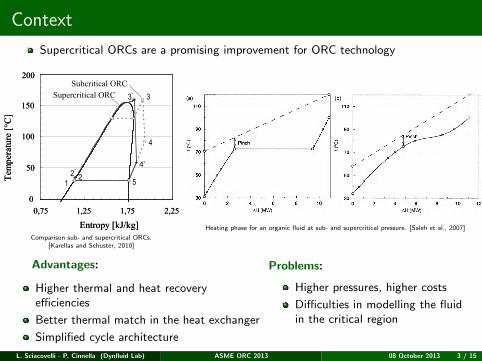
Supercritical ORCs are a promising improvement for ORC technology

Int. J. of Thermodynamics, Vol. 11 (No. 3) 102

Water

Organic Fluid

p1

p1=2 bar

p2=10 bar

p3=30 bar

p3

p2

Water

Organic Fluid

p1

p1=2 bar

p2=10 bar

p3=30 bar

p3

p2

C. P.

C. P.

0

100

200

300

400

Tem

perature [°C]

Entropy [kJ/kg]

0,0 2,0 4,0 6,0 8,0

Organic Fluid

Water p3=30 bar

p1

p2

p3 p2=10 bar

p1=2 bar

Figure 1. T-S Diagram for organic fluid and

water.

average temperature level. In reality such big

superheating as shown in the diagram would not

be realized due to the tremendous heat exchange

area needed due to the low heat-exchange

coefficient for the gaseous phase.

supercritical ORC

subcritical ORC

2

1

3‘

3

3‘‘

3

5

4

supercritical ORC

subcritical ORC

2

1

3‘

3

3‘‘

3

5

4

Entropy [kJ/kg]

0,75 1,25 1,75 2,25

0

50

100

150

200

Tem

perature [°C]

Subcritical ORC

Supercritical ORC ’

4’

2’

supercritical ORC

subcritical ORC

2

1

3‘

3

3‘‘

3

5

4

supercritical ORC

subcritical ORC

2

1

3‘

3

3‘‘

3

5

4

Entropy [kJ/kg]

0,75 1,25 1,75 2,25

0

50

100

150

200

Tem

perature [°C]

Subcritical ORC

Supercritical ORC ’

4’

2’

Figure 2. Sub- and supercritical ORC. Example

of R245fa.

The thermal efficiency of the cycle is

defined as follows:

oilThermal

mech

thQ

P

−

=&

η (1)

Pmech is the net mechanical power produced

with the ORC process (which will be assumed as

equal the net electrical power). This power

output is analogue to the enthalpy fall in the

turbine minus the enthalpy rise in the pump:

)()(~ 1243 hhhhPmech −−− (2)

The heat input to the ORC process is done

usually with the help of the thermal oil and is

analogue to:

)(~ 23 hhQ oilThermal −−

& (3)

h1, h2, h3 and h4 are the specific enthalpies

according to Figure 2.

In the case of supercritical process, the

enthalpy fall (h3’-h4’) is much higher than in the

subcritical one, whereas the feed pump’s

additional specific work to reach supercritical

pressure, which corresponds to the enthalpy rise

(h2’-h2), is very low.

Therefore, according to equation (1), the

efficiency of the process is higher in the case of

supercritical ORC parameters and this fact

provides new frontiers in the investigation of

ORC applications.

For the heat exchange system that transfers

the heat from the heat source to the organic fluid,

the efficiency is defined by the following

equation:

sourceHeat

fluidOrganic

HExQ

Q

−

=&

&

η (4)

Finally, the efficiency of the whole system

is defined as follows:

thHEx

sourceHeat

mech

SystemQ

Pηηη ⋅==

−&

(5)

The above presented efficiencies will be

used for the qualitative analysis of the ORC

applications which will be described in this

paper.

2. Cycle design

2.1 Organic Fluids

The first step when designing an ORC cycle

application is the choice of the appropriate

working fluid. The working fluids which can be

used are well known mainly from refrigeration

technologies. The selection of the fluid is done

according to the process parameters of the cycle.

According to the critical pressure and

temperature, as well as the boiling temperature in

various pressures, the appropriate fluid which

provides the highest thermal and system

efficiency has to be selected. However, the

thermodynamic parameters of the fluid are not

the only criteria to select them for efficient

Comparison sub- and supercritical ORCs.[Karellas and Schuster, 2010]

Heating phase for an organic fluid at sub- and supercritical pressure. [Saleh et al., 2007]

Advantages: Problems:

Higher thermal and heat recoveryefficiencies

Better thermal match in the heat exchanger

Simplified cycle architecture

Higher pressures, higher costs

Difficulties in modelling the fluidin the critical region


Thermodynamic Modelling

Candidate working fluids: R134a, R245fa, CO2

Dense gas behavior modeled through EoS based on Helmholtz free energy Φ

Reduced parameters δ = ρ/ρc and τ = Tc/T as indipendent variablesEoS composed by ideal and residual part

Φ(δ, τ) = Φ0(δ, τ) + Φr(δ, τ)

Φ0(δ, τ) = ln δ + a1 ln τ +

M1∑m=1

amτjm +

M2∑m=M1+1

am ln[1− exp(−umτ)]

Φr(δ, τ) =

M3∑m=M2+1

amδimτ jm +

M4∑m=M3+1

amδimτ jm exp(−δkm)+

M5∑m=M4+1

amδimτ jm exp[−αm(δ − εm)2 − βm(τ − γm)2]

The ideal part requires an ancillary equation for the ideal-gas heat capacity

Coefficients, exponents and number of terms calibrated on experimental data bymeans of an optimization algorithm [Setzmann and Wagner, 1989]


Thermodynamic Modelling

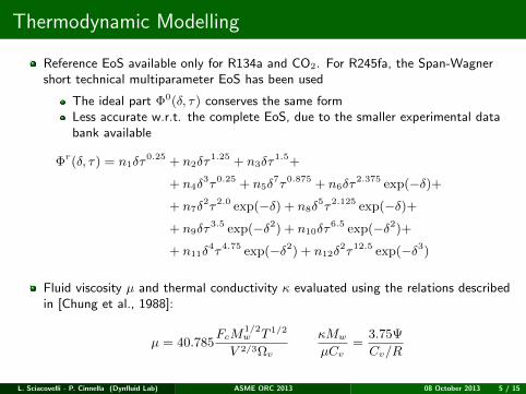
Reference EoS available only for R134a and CO2. For R245fa, the Span-Wagnershort technical multiparameter EoS has been used

The ideal part Φ0(δ, τ) conserves the same formLess accurate w.r.t. the complete EoS, due to the smaller experimental databank available

Φr(δ, τ) = n1δτ0.25 + n2δτ

1.25 + n3δτ1.5+

+ n4δ3τ0.25 + n5δ

7τ0.875 + n6δτ2.375 exp(−δ)+

+ n7δ2τ2.0 exp(−δ) + n8δ

5τ2.125 exp(−δ)+

+ n9δτ3.5 exp(−δ2) + n10δτ

6.5 exp(−δ2)+

+ n11δ4τ4.75 exp(−δ2) + n12δ

2τ12.5 exp(−δ3)

Fluid viscosity µ and thermal conductivity κ evaluated using the relations describedin [Chung et al., 1988]:

µ = 40.785FcM

1/2w T 1/2

V 2/3Ωv

κMw

µCv=

3.75Ψ

Cv/R


Numerical method

Equations of motion:

∫Ω(t)

ω dΩ+

∮∂Ω(t)

(fe−fv)·n dS = s, ω =

ρρvρE

fe =

ρvρvv + pIρvH

fv =

0τ

τ · v − q

with p = p(e(ω), ρ(ω)) or

Caloric EoS: e = e(T (ω), ρ(ω))

Thermal EoS: p = p(T (ω), ρ(ω))

Spatial discretization:

Structured finite-volume approach

Third-order accuracy, centered,conservative scheme with artificialviscosity

Extension to curvilinear grid usingweighting coefficients that take intoaccount mesh deformations

Time integration:

Four-stage Runge-Kutta method withimplicit residual smoothing

Turbulence modeling:

Algebraic Model: Baldwin-Lomax

One-equation Model: Spalart-Allmaras


Simulation setup

Appel à Projets R&D « Amélioration de la performance énergétique des procédés et

utilités industriels» Rapport d’avancement n.3- Partenaire n° 1—ARTS

Projet SURORC

8/27

Stage 1 Stage N

Inlet Outlet

Periodicity

Periodicity

Periodicity

Periodicity

Periodicity

Periodicity

Periodicity

Periodicity

Periodicity

Periodicity

Periodicity

Periodicity

Mixing planeMixing plane Mixing plane

Wall

Wall

Wall

Wall

Wall

Wall

Non conformal joins

Figure 1. Schématisation des domaines de calcul et des conditions aux limites

Les Fig.2-4 montrent l’évolution sur le diagramme T-s des conditions thermodynamiques au

cours de la détente pour le trois fluides considérés. Les triangles indiquent le début et la fin de

chaque étage. La position de la courbe de détente par rapport à la courbe de coexistence

liquide/vapeur révèle trois situations différentes: pour le R134a (Fig.2), dans le premier étage

on a des conditions super- et transcritiques, tandis que le reste de l'expansion est sous-critique.

L'expansion du R245fa (Fig.3) est sous-critique et se produit en correspondance de la partie

de la courbe de vapeur saturée à pente positive, là où le R245fa se comporte donc comme un

fluide sechant. L'état thermodynamique à l’entrée du premier étage est proche de la zone de

saturation. Complètement différent est la situation du CO2 (Fig.4), pour laquelle toute la

détente se passe dans des conditions largement supercritiques.

La géométrie étudiée pour le profil NACA A3K7 est montrée en Fig.4. Le

maillage utilisé est composé par 272x32 cellules ; comme le même profil est

utilisé aussi bien pour les aubes du rotor que du stator, la grille du rotor est

obtenue en inversant celle du stator. La distance stator-rotor est 0.2c, ou c est la

chorde axiale (égale à 3cm).

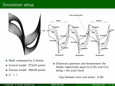
Mesh composed by C-blocks

Inviscid model: 273x33 points

Viscous model: 389x49 points

y+ = 1

Distances upstream and downstream theblades respectively equal to 0.15c and 0.2c,being c the axial chord

Gap between rotor and stator: 0.35c


Simulation setup

R134a R245fa CO2

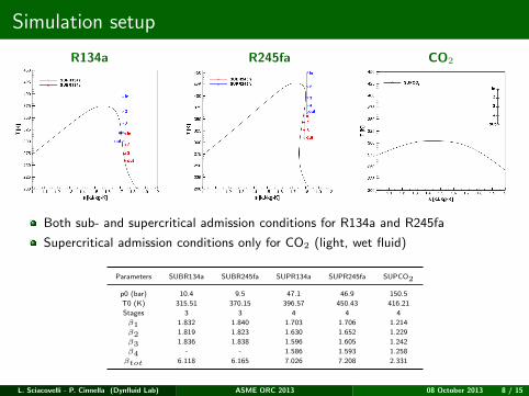
Both sub- and supercritical admission conditions for R134a and R245fa

Supercritical admission conditions only for CO2 (light, wet fluid)

Parameters SUBR134a SUBR245fa SUPR134a SUPR245fa SUPCO2

p0 (bar) 10.4 9.5 47.1 46.9 150.5

T0 (K) 315.51 370.15 396.57 450.43 416.21

Stages 3 3 4 4 4

β1 1.832 1.840 1.703 1.706 1.214

β2 1.819 1.823 1.630 1.652 1.229

β3 1.836 1.838 1.596 1.605 1.242

β4 - - 1.586 1.593 1.258

βtot 6.118 6.165 7.026 7.208 2.331


Results: inviscid model

Turbine stage efficiencies for the inviscid model.

Stage SUBR134a SUBR245fa SUPR134a SUPR245fa SUPCO2

1 95.07 92.55 94.63 91.12 98.72

2 94.03 89.59 95.80 91.99 98.27

3 92.94 88.36 95.87 92.45 99.86

4 - - 98.41 93.62 99.11

Different isentropic efficiencies mainly due to different fluid dynamic behaviour

Important parameter to evaluate the results: Fundamental derivative of GasDynamics [Thompson, 1971]:

Γ = 1 +ρ

a

(∂a

∂ρ

)s

⇒ ∂a

a= (Γ− 1)

∂ρ

ρ


Results: viscous model

Turbine stage efficiencies for the B-L model.


1 84.21 78.55 85.72 82.04 89.67

2 83.99 78.41 86.23 82.15 89.91

3 83.86 77.28 86.91 82.56 90.04

4 - - 87.64 82.99 90.11

Turbine stage efficiencies for the S-A model.


1 84.13 80.61 84.68 81.98 89.63

2 83.87 78.76 85.98 82.13 89.85

3 83.45 76.21 86.24 82.23 89.92

4 - - 87.53 82.35 90.04

Efficiencies about 10% lower w.r.t inviscid case

Baldwin-Lomax predicts an efficiency about 1% higher than Spalart-Allmaras


Turbulence model comparison - R134a 1st stage rotor

Wall pressure on suction side slightly lower for B-L model

Friction Coefficient higher for S-A model

Dimensionless wall pressure Friction coefficient

Overall S-A efficiency lower

Results presented in the following are computed with B-L


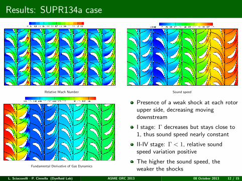
Results: SUPR134a case

Relative Mach Number Sound speed

Fundamental Derivative of Gas Dynamics

Presence of a weak shock at each rotorupper side, decreasing movingdownstream

I stage: Γ decreases but stays close to1, thus sound speed nearly constant

II-IV stage: Γ < 1, relative soundspeed variation positive

The higher the sound speed, theweaker the shocks


Results: SUBR245fa vs SUBR134a

Γ ≈ 1

Sound speednearly constant

Stronger shocks

Lowerefficiencies

R245fa

Relative Mach Number

R134a

Relative Mach Number

Better behaviorfor R134a

Fundamental Derivative of Gas Dynamics Fundamental Derivative of Gas Dynamics


Results: SUPCO2 case

Relative Mach NumberSound speed

Fundamental Derivative of Gas Dynamics

Supercritical expansion, Γ > 1 always

Light fluid: high sound speed

Absence of shocks: maximumefficiency in viscous and inviscid cases

Higher plant costs due to higher meanpressures of the cycle


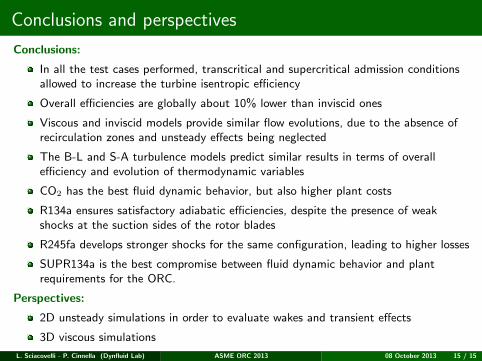
Conclusions and perspectives

Conclusions:

In all the test cases performed, transcritical and supercritical admission conditionsallowed to increase the turbine isentropic efficiency

Overall efficiencies are globally about 10% lower than inviscid ones

Viscous and inviscid models provide similar flow evolutions, due to the absence ofrecirculation zones and unsteady effects being neglected

The B-L and S-A turbulence models predict similar results in terms of overallefficiency and evolution of thermodynamic variables

CO2 has the best fluid dynamic behavior, but also higher plant costs

R134a ensures satisfactory adiabatic efficiencies, despite the presence of weakshocks at the suction sides of the rotor blades

R245fa develops stronger shocks for the same configuration, leading to higher losses

SUPR134a is the best compromise between fluid dynamic behavior and plantrequirements for the ORC.

Perspectives:

2D unsteady simulations in order to evaluate wakes and transient effects

3D viscous simulations


THANKS FOR THE ATTENTION


References

Chen, H., Goswami, D., and Stefanakos, E. (2010). A review of thermodynamiccycles and working fluids for the conversion of low-grade heat. Renewable andSustainable Energy Reviews, 14(9):3059–3067.

Chung, T. H., Ajlan, M., Lee, L. L., and Starling, K. E. (1988). Generalizedmultiparameter correlation for nonpolar and polar fluid transport properties.Industrial & engineering chemistry research, 27(4):671–679.

Karellas, S. and Schuster, A. (2010). Supercritical fluid parameters in OrganicRankine Cycle applications. International Journal of Thermodynamics,11(3):101–108.

Saleh, B., Koglbauer, G., Wendland, M., and Fischer, J. (2007). Working fluids forlow-temperature Organic Rankine Cycles. Energy, 32(7):1210–1221.

Setzmann, U. and Wagner, W. (1989). A new method for optimizing the structureof thermodynamic correlation equations. International Journal of Thermophysics,10(6):1103–1126.

Thompson, P. (1971). A Fundamental Derivative in Gas Dynamics. Physics ofFluids, 14:1843–1849.


Supercritical ORCs

3. Working fluid properties and selection criteria

The working fluid plays a key role in the cycle. A working fluidmust not only have the necessary thermo-physical properties thatmatch the application but also possess adequate chemical stabilityin the desired temperature range. The fluid selection affects systemefficiency, operating conditions, environmental impact andeconomic viability. Selection criteria are set out in this sectionto locate the potential working fluid candidates for different cyclesat various conditions.

3.1. Thermodynamic and physical properties

In this section, types of working fluids, fluid density, specificheat, latent heat, critical point, thermal conductivity, specificvolume at saturation (condensing) conditions, as well as saturationvolumes are analyzed and discussed. The desired properties arethen discussed for the screening of potential working fluids.

3.1.1. Types of working fluids

It has been mentioned in Section 2 that a working fluid can beclassified as a dry, isotropic, or wet fluid depending on the slope ofthe saturation vapor curve on a T–s diagram (dT/ds). Since the valueof dT/ds leads to infinity for isentropic fluids, the inverse of theslope, (i.e. ds/dT,) is used to express how ‘‘dry’’ or ‘‘wet’’ a fluid is. Ifwe define j = ds/dT, the type of working fluid can be classified bythe value of j, i.e. j > 0: a dry fluid (e.g. pentane), j 0: anisentropic fluid (e.g. R11), and j < 0: a wet fluid (e.g. water). Fig. 4shows the three types of fluids in a T–s diagram.

Liu et al. derived an expression to compute j, which is: [62]

j ¼ C p

TH ððn TrHÞ=ð1 TrHÞÞ þ 1

T2H

DHH (1)

where j(ds/dT) denotes the inverse of the slope of saturated vaporcurve on T–s diagram, n is suggested to be 0.375 or 0.38 [63], TrH

(=TH/TC) denotes the reduced evaporation temperature, and DHH isthe enthalpy of vaporization.

It needs to be mentioned that Eq. (1) is developed throughsimplifications. The reliability of the equation was verified at thefluids’ normal boiling points by Liu et al. [62]. However, ourcalculations based on the definition of the slope (ds/dT) show thatlarge deviations can occur when using Eq. (1) at off-normal boilingpoints. Therefore, it is recommended to use the entropy andtemperature data directly to calculate j if their values are available.

Isentropic or dry fluids were suggested for organic Rankinecycle to avoid liquid droplet impingent in the turbine blades duringthe expansion. However, if the fluid is ‘‘too dry,’’ the expanded

vapor will leave the turbine with substantial ‘‘superheat’’, which isa waste and adds to the cooling load in the condenser. The cycleefficiency can be increased using this superheat to preheat theliquid after it leaves the feed pump and before it enters the boiler.An organic Rankine cycle with an isentropic working fluid is shownin aforesaid Fig. 1(b).

There is still a great need to find proper working fluids forsupercritical Rankine cycles. Fig. 5 shows a dry fluid, propyne, and awet fluid pentane used in supercritical Rankine cycles. If theexpansion is carried out such that the expansion does not go intothe two-phase region (the dashed lines in Fig. 5(a) and (b)), dryfluids may leave the turbine with substantial amount of superheat,which adds to the burden for the condensation process or arecovery system is needed. Wet fluids, on the other hand, will needhigher turbine inlet temperature to avoid two-phase region butthere is less concern about desuperheating after the expansion. Ifthe process is allowed to pass through the two-phase region (thesolid lines in Fig. 5), the dry fluid can still leave the turbine atsuperheated state, while the wet fluid stays in the two-phaseregion at the turbine exit. Bakhtar et al. [64–68] found that for awet fluid, such as, water, the fluid first subcools and then nucleatesto become a two-phase mixture. The formation and behavior of theliquid in the turbine create problems that would lower theperformance of the turbine. For dry fluids, Goswami et al. [69] andDemuth [70,71] found that only extremely fine droplets (fog) wereformed in the two-phase region and no liquid was actually formedto damage the turbine before it started drying during theexpansion. Demuth [70] also found that the turbine performanceshould not degrade significantly as a result of the turbineexpansion process passing through and leaving the moistureregion if no condensation occurs. Meanwhile, potential gains in thenet fluid effectiveness on the order of 8% can be achieved resulting

[(Fig._4)TD$FIG]

Fig. 4. Three types of working fluids: dry, isentropic, and wet.

[(Fig._5)TD$FIG]

Fig. 5. T–s diagram shows a dry fluid and a wet fluid used in supercritical cycles. (a)

Pentane as the working fluid. (b) Propyne as the working fluid.

H. Chen et al. / Renewable and Sustainable Energy Reviews 14 (2010) 3059–30673062

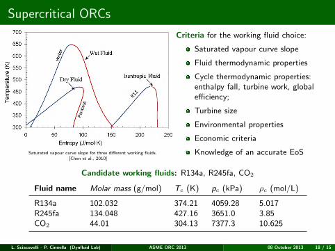
Saturated vapour curve slope for three different working fluids.[Chen et al., 2010]

Criteria for the working fluid choice:

Saturated vapour curve slope

Fluid thermodynamic properties

Cycle thermodynamic properties:enthalpy fall, turbine work, globalefficiency;

Turbine size

Environmental properties

Economic criteria

Knowledge of an accurate EoS

Candidate working fluids: R134a, R245fa, CO2

Fluid name Molar mass (g/mol) Tc (K) pc (kPa) ρc (mol/L)

R134a 102.032 374.21 4059.28 5.017R245fa 134.048 427.16 3651.0 3.85CO2 44.01 304.13 7377.3 10.625


Numerical study of multistage transcritical ORC axial...

Documents

Transcript of Numerical study of multistage transcritical ORC axial...