Numerical Simulation of the Fluid Dynamics of 3D Free Surface

Flows with an Upwind Convection Scheme

Laıs Correa, Valdemir Garcia Ferreira

Depto. de Matematica Aplicada e Estatıstica, ICMC, USP,

13566-590, Sao Carlos, SP

E-mail: lacorrea@icmc.usp.br, pvgf@icmc.usp.br

Abstract: A high resolution bounded upwind convection scheme, namely EPUS (Eight-degreePolynomial Upwind Scheme), is presented for computing 3D incompressible fluid flows involvingmoving free surfaces. The scheme is based on the CBC (Convection Boundedness Criterion)and TVD (Total Variation Diminishing) stability criteria. In NV (Normalized Variables), theEPUS scheme is applied in two problems that demonstrate its utility in solving complex PDE.

Key words: Upwind Schemes, Navier-Stokes Equations, Numerical Simulation, Free Surface

1. Development of a three points upwind scheme

The three points upwind strategy was utilized by the development of the EPUS scheme, thatis the convective terms are approximated according to the sign of a convection velocity for atransported variable φf . The computational stencil is composed by three nodes: the downstreamD, the upstream U and the remote-upstream R. Figure 1 illustrates the position of these nodes.

DUR

φf

Vf

D U R

φf

Vf

Figure 1: Computational nodes D, U and R and velocity Vf for the convected variable φf

A scheme that takes into account the upwind strategy can be write in the following form

φf = φf (D,U,R). (1)

In order to simplify this functional relationship, the NV of Leonard [7] was employed:

φ() =φ() − φR

φD − φR. (2)

With this definition, one can see that any convection scheme using three computational nodescan be rewritten in a more simplified form

φf = φf (φU ). (3)

Representative examples are the (diffusive) FOU (First Order Upwind) scheme

φf = φU (4)

and the (dispersive) QUICK scheme

φf =3

4φU +

3

8. (5)

557

ISSN 1984-8218

Leonard showed that for derivating a high order (nonlinear or piecewise linear) monotonicscheme, the following conditions must be satisfyed: it must pass through points O(0, 0) andP (1, 1) (both conditions for monotonicity); pass through point Q(0.5, 0.75) (for reaching secondorder of accuracy) and pass through point Q with inclination of 0.75 (for reaching third order ofaccuracy). Further more, Leonard recommends that for values of φU < 0 or φU > 1, one mustconsider the FOU scheme. For stability of the calculations using the EPUS scheme, two criteriawere employed: CBC of Gaskell and Lau [5] and TVD of Harten [6].

2. EPUS scheme

For the development of the EPUS scheme (see more details in [3]), we considered part of aneight-degree polynomial in the interval [0, 1], and out of it we use the FOU scheme

φf (φU ) =

{

a8φ8U+a7φ

7U+a6φ

6U+a5φ

5U+a4φ

4U+a3φ

3U+a2φ

2U+a1φU+a0, se φU ∈ [0, 1],

φU , se φU /∈ [0, 1].(6)

For determining the coefficients ai, i = 0, ..., 8, we imposed the four conditions of Leonardpresented previously plus the conditions that the polynomial is a C2 class function (followingthe ideas of Lin and Chieng [8]) and that the coefficient a3 is a free parameter, say λ. Thedifferentiabily conditions were imposed at the points (0, 0) and (1, 1), with the same values ofthe first and second derivatives of the FOU scheme. In summary, the EPUS scheme in NV andwith a free parameter λ is defined by

φf =

−4(λ− 24)φ8U + 16(λ − 23)φ7U + (528 − 25λ)φ6U+

+(19λ− 336)φ5U + (80− 7λ)φ4U + λφ3U + φU , if φU ∈ [0, 1],

φU , if φU /∈ [0, 1].

(7)

The corresponding flux limiter function, ψf , for the EPUS scheme is obtained by using thegeneral approximation (see, for example, [3])

φf = φU +1

2ψf (1− φU ), (8)

where rf is the ratio of consecutive gradients (a type of sensor), given by

rf =φU

1− φU. (9)

The EPUS flux limiter is derived from Eqs. (7), (8) and (9), and the result is

ψ(rf ) = max

{

0,0.5(|rf |+ rf )[(2λ− 32)r4f + (160 − 4λ)r3f + 2λr2f ]

(1 + |rf |)7

}

. (10)

One can show that the EPUS scheme is TVD for the free parameter λ into the interval[16,95] (see details in [3]). Another property possessed by the EPUS scheme is that the choiceof the parameter λ is dependent of the problem. In general, the values of λ = 16 and 95 haveprovided useful results for various numerical tests. For example, it has been observed that theEPUS scheme with λ = 16 has good performance in problems with smooth initial conditions,while with λ = 95 EPUS provided good resolution near to extreme points, high gradients anddiscontinuities.

558

ISSN 1984-8218

3. Numerical results

The performance of the EPUS scheme is assessed in this paper in three problems, namely:one convergence test for the 1D advection equation and two numerical simulations of the 3D freesurface flows modeled by the Navier-Stokes equations, Broken-dam and jet buckling problems.

3.1 1D Advection equation - A convergence test

Before of applying the EPUS scheme for solving 3D free surface flows, a convergence test ispresented. For this, the 1D advection equation given by

∂u

∂t+ a

∂u

∂x= 0, x ∈ [−π, π], (11)

is considered, where a > 0 (constant) is the advection velocity of the convected variable u =u(x, t). The initial condition u(x, 0) = sin(x) and periodic boundary condition are applied.

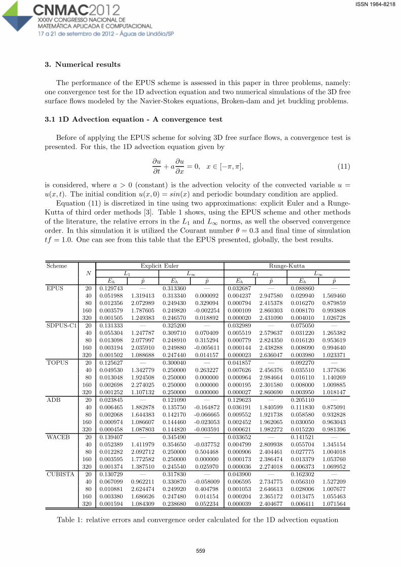
Equation (11) is discretized in tine using two approximations: explicit Euler and a Runge-Kutta of third order methods [3]. Table 1 shows, using the EPUS scheme and other methodsof the literature, the relative errors in the L1 and L∞ norms, as well the observed convergenceorder. In this simulation it is utilized the Courant number θ = 0.3 and final time of simulationtf = 1.0. One can see from this table that the EPUS presented, globally, the best results.

Scheme Explicit Euler Runge-Kutta

N L1 L∞ L1 L∞

Eh p Eh p Eh p Eh p

EPUS 20 0.129743 — 0.313360 — 0.032687 — 0.088860 —

40 0.051988 1.319413 0.313340 0.000092 0.004237 2.947580 0.029940 1.569460

80 0.012356 2.072989 0.249430 0.329094 0.000794 2.415378 0.016270 0.879859

160 0.003579 1.787605 0.249820 -0.002254 0.000109 2.860303 0.008170 0.993808

320 0.001505 1.249383 0.246570 0.018892 0.000020 2.431090 0.004010 1.026728

SDPUS-C1 20 0.131333 — 0.325200 — 0.032989 — 0.075050 —

40 0.055304 1.247787 0.309710 0.070409 0.005519 2.579637 0.031220 1.265382

80 0.013098 2.077997 0.248910 0.315294 0.000779 2.824350 0.016120 0.953619

160 0.003194 2.035910 0.249880 -0.005611 0.000144 2.438288 0.008090 0.994640

320 0.001502 1.088688 0.247440 0.014157 0.000023 2.636047 0.003980 1.023371

TOPUS 20 0.125627 — 0.300040 — 0.041857 — 0.092270 —

40 0.049530 1.342779 0.250000 0.263227 0.007626 2.456376 0.035510 1.377636

80 0.013048 1.924508 0.250000 0.000000 0.000964 2.984664 0.016110 1.140269

160 0.002698 2.274025 0.250000 0.000000 0.000195 2.301580 0.008000 1.009885

320 0.001252 1.107132 0.250000 0.000000 0.000027 2.860690 0.003950 1.018147

ADB 20 0.023845 — 0.121090 — 0.129623 — 0.205110 —

40 0.006465 1.882878 0.135750 -0.164872 0.036191 1.840599 0.111830 0.875091

80 0.002068 1.644383 0.142170 -0.066665 0.009552 1.921738 0.058580 0.932828

160 0.000974 1.086607 0.144460 -0.023053 0.002452 1.962065 0.030050 0.963043

320 0.000458 1.087803 0.144820 -0.003591 0.000621 1.982272 0.015220 0.981396

WACEB 20 0.139407 — 0.345490 — 0.033652 — 0.141521 —

40 0.052389 1.411979 0.354650 -0.037752 0.004799 2.809938 0.055704 1.345154

80 0.012282 2.092712 0.250000 0.504468 0.000906 2.404461 0.027775 1.004018

160 0.003595 1.772582 0.250000 0.000000 0.000173 2.386474 0.013379 1.053760

320 0.001374 1.387510 0.245540 0.025970 0.000036 2.274018 0.006373 1.069952

CUBISTA 20 0.130729 — 0.317830 — 0.043900 — 0.162302 —

40 0.067099 0.962211 0.330870 -0.058009 0.006595 2.734775 0.056310 1.527209

80 0.010881 2.624474 0.249920 0.404798 0.001053 2.646613 0.028006 1.007677

160 0.003380 1.686626 0.247480 0.014154 0.000204 2.365172 0.013475 1.055463

320 0.001594 1.084309 0.238680 0.052234 0.000039 2.404677 0.006411 1.071564

Table 1: relative errors and convergence order calculated for the 1D advection equation

559

ISSN 1984-8218

3.2 3D Navier-Stokes equations

The performance of the EPUS scheme is assessed in 3D fluid flows modeled by the Navier-Stokes equations

∂ui∂t

+∂(uiuj)

∂xj= − ∂p

∂xi+

1

Re

∂

∂xj

(

∂ui∂xj

)

+1

Fr2gi, i = 1, 2, 3 (12)

∂ui∂xi

= 0, (13)

in which ui is the component of velocity vector in xi direction, g = (gx, gy, gz)T is the acceleration

due to gravity, p represents the pressure, and the dimensionless parameters are Re = U0L0/ν(Reynolds number) and Fr = U0

√L0g (Froude number), with ν being the kinematic viscosity

(constant) and U0 and L0 the characteristic scales for velocity and length, respectively. For solv-ing numerically these equations, we have used the Freeflow code of Castelo et al. [1] equippedwith the EPUS upwind scheme. In particular, two well recognized phenomena, namely brokendam and jet buckling, are simulated. The results with the EPUS scheme are presented below.

3.2.1 Broken dam

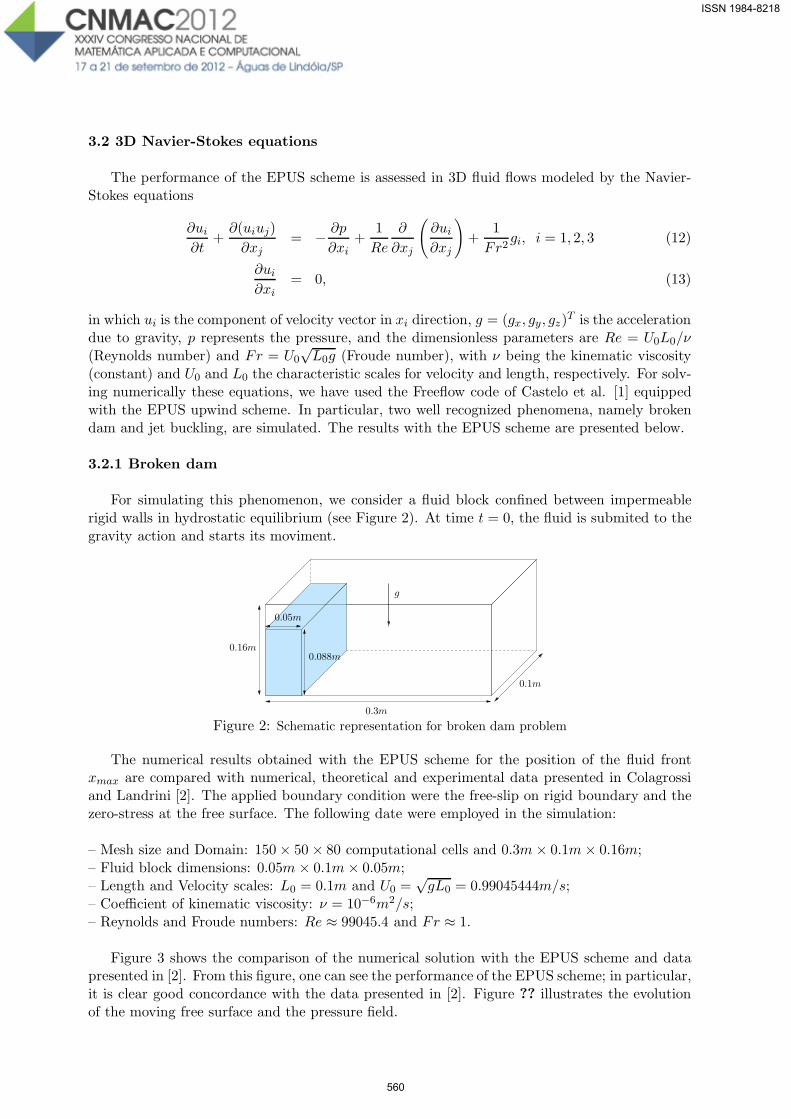
For simulating this phenomenon, we consider a fluid block confined between impermeablerigid walls in hydrostatic equilibrium (see Figure 2). At time t = 0, the fluid is submited to thegravity action and starts its moviment.

g

0.16m

0.1m

0.3m

0.05m

0.088m

Figure 2: Schematic representation for broken dam problem

The numerical results obtained with the EPUS scheme for the position of the fluid frontxmax are compared with numerical, theoretical and experimental data presented in Colagrossiand Landrini [2]. The applied boundary condition were the free-slip on rigid boundary and thezero-stress at the free surface. The following date were employed in the simulation:

– Mesh size and Domain: 150× 50 × 80 computational cells and 0.3m× 0.1m× 0.16m;– Fluid block dimensions: 0.05m × 0.1m× 0.05m;– Length and Velocity scales: L0 = 0.1m and U0 =

√gL0 = 0.99045444m/s;

– Coefficient of kinematic viscosity: ν = 10−6m2/s;– Reynolds and Froude numbers: Re ≈ 99045.4 and Fr ≈ 1.

Figure 3 shows the comparison of the numerical solution with the EPUS scheme and datapresented in [2]. From this figure, one can see the performance of the EPUS scheme; in particular,it is clear good concordance with the data presented in [2]. Figure ?? illustrates the evolutionof the moving free surface and the pressure field.

560

ISSN 1984-8218

0 0,5 1 1,5 2 2,50

1

2

3

4

5

6

Num. Sol. SPHNum. Sol. BEMNum. Sol. Level SetTheo. Sol. RitterExp. Martin e Moyce

EPUS

t√

g/a

xmax/a

Figure 3: Comparison of the solutions for the 3D broken dam problem

3.2.2 Jet buckling

This problem is characterized by the formation of the physical oscillations of the fluid duringits moviment. The oscillations occur when a highly viscous fluid (or low Reynolds number) andunder the gravity action, impinges perpendiculary on an impermeable rigid wall (see Figure 4).It is worth noting, that although this problem does not reflect the importance of the EPUS, it issimulated with the objective to show that the scheme is also useful for solving complex problemsat low Reynolds numbers.

Inflow

Rigid surface

hi

d

H

Figure 4: Schematic illustration for the jet buckling problem

In the last years, has been a great challenge to understand this phenomenon (see, for exam-ple, [3]). From the experiments and studies, was possible observe that the oscillations occourwhen two relations are complied. One these relations is that the ratio H/d (see in Figure 4)must be greater than critic value (H/d)c = 7.2. The other relation say that the adimensionalRe must be smaller than critic value Rec = 1.2 (for more details, see Cruickshank [4]). For thesimulation of this phenomenon, we consider the no-slip condition on the rigid boundary andzero-stress on the free surface. The following data were employed in the computation:

– Mesh size and Domain: 100× 100 × 123 computational cells and 1m× 1m× 1.23m;– Inflow diameter and height: d = 0.04m and hi = 0.2m;– Lenght and Velocity scales: L0 = 2d = 0.08m and U0 = 1m/s;– Coefficient of kinematic viscosity: ν = 0.278m2/s;– Reynolds and Froude numbers: Re ≈ 0.3 and Fr =≈ 1.1.

561

ISSN 1984-8218

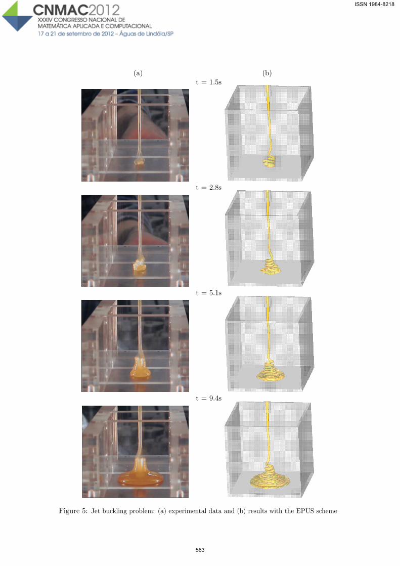
One can see observe, from these imput data, that the relations for the occurrence of oscillationsare satisfied; in fact, H/d = 25 > 7.2 and Re = 0.288 < 1.2. Some results are presented in theFigure 5, where it is compared the numerical solution obatained with the EPUS scheme and theexperimental results presented in [9]. One can clearly see that the EPUS scheme simulated thebuckling phenomenon and that it provides results very closer to the experimental data.

4. Conclusion

We presented the EPUS scheme, a polynomial upwind convection scheme for numericalsimulation of the fluid dynamics of 3D free surface flows. The scheme was developed based onthe NV formulation and on the TVD/CBC stability criteria. In this article, the performance ofthe EPUS scheme was assessed in a convergence order test for the 1D scalar advection equationand by solving the broken dam and jet buckling problems modeled by the 3D Navier-Stokesequations. The obtained results showing that the EPUS scheme is a useful high resolutionupwind scheme for complex flows.

5. Acknowledgments

We gratefully acknowledge the support provided by the FAPESP (Grant 2010/16865-2) andCNPq (Grant 306808/2011-0). This work was also carried out in the framework of the InstitutoNacional de Ciencia e Tecnologia em Medicina Assistida por Computacao Cientıfica (CNPq,Brazil).

References

[1] A. Castelo, M. F. Tome, S. McKee, J. A. Cuminato and C. N. L. Cesar, Freeflow: anintegrated simulation system for three-dimensional free surface flows, Journal of Computersand Visualization in Science, 2, (2000) 1-12.

[2] A. Colagrossi and M. Landrini, Numerical simulation of interfacial flows by smoothed par-ticle hydrodynamics, Journal Computation Physics, 191, (2003) 448-475.

[3] L. Correa. “Um novo esquema upwind de alta resolucao para equacoes de conservacao naoestacionarias dominadas por conveccao”, Dissertacao de mestrado, ICMC-USP, 2011.

[4] J. O. Cruickshank, Low Reynolds number instabilities in stagnating jet flows, Journal ofFluid Mechanics, 193, (1987) 111-127.

[5] P. H. Gaskell and A. K. C. Lau, Curvature-compensated convective transport: SMART,a new boundedness preserving transport algorithm, International Journal for NumericalMethods in Fluids, 8, (1988) 617-641.

[6] A. Harten, High resolution schemes for hyperbolic conservation laws, Journal of Computa-tional Physics, 49, (1983) 357-393.

[7] B. P. Leonard, Simple high-accuracy resolution program for convective modeling of discon-tinuities, International Journal for Numerical Methods in Fluids, 8, (1988) 1291-1318.

[8] H. Lin and C. C. Chieng, Characteristic-based flux limiters of an essentially third-orderflux-splitting method for hyperbolic conservation laws, International Journal for NumericalMethods in Fluids, 13, (1991) 287-307.

[9] J.M. Nobrega, O.S. Carneiro, F.T. Pinho, G.S. Paulo, M.F. Tome, A. Castelo and J.A.Cuminato, The phenomenon of jet buckling: Experimental results and numerical predic-tions, The Polymer Processing Society 23rd Annual Meeting.

562

ISSN 1984-8218

(a) (b)t = 1.5s

t = 2.8s

t = 5.1s

t = 9.4s

Figure 5: Jet buckling problem: (a) experimental data and (b) results with the EPUS scheme

563

ISSN 1984-8218