Numerical Simulations in Fluid Dynamics using GPU a Practical
MSc Energy Enginering
Numerical methods in
heat transfer and fluid dynamics
MASTER THESIS
Author: Sergio Zavaleta Camacho
Director: Carlos David Pérez Segarra
Announcement: September 2017
Escola Tècnica Superior d’Enginyeria Industrial de Barcelona
Numerical methods in heat transfer and fluid dynamics Page 1
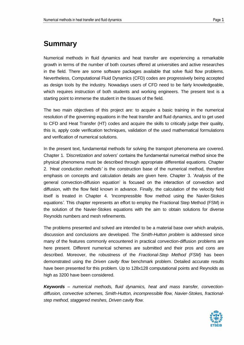
Summary
Numerical methods in fluid dynamics and heat transfer are experiencing a remarkable
growth in terms of the number of both courses offered at universities and active researches
in the field. There are some software packages available that solve fluid flow problems.
Nevertheless, Computational Fluid Dynamics (CFD) codes are progressively being accepted
as design tools by the industry. Nowadays users of CFD need to be fairly knowledgeable,
which requires instruction of both students and working engineers. The present text is a
starting point to immerse the student in the tissues of the field.
The two main objectives of this project are: to acquire a basic training in the numerical
resolution of the governing equations in the heat transfer and fluid dynamics, and to get used
to CFD and Heat Transfer (HT) codes and acquire the skills to critically judge their quality,
this is, apply code verification techniques, validation of the used mathematical formulations
and verification of numerical solutions.
In the present text, fundamental methods for solving the transport phenomena are covered.
Chapter 1. ‘Discretization and solvers’ contains the fundamental numerical method since the
physical phenomena must be described through appropriate differential equations. Chapter
2. ‘Heat conduction methods’ is the construction base of the numerical method, therefore
emphasis on concepts and calculation details are given here. Chapter 3. ‘Analysis of the
general convection-diffusion equation’ is focused on the interaction of convection and
diffusion, with the flow field known in advance. Finally, the calculation of the velocity field
itself is treated in Chapter 4. ‘Incompressible flow method using the Navier-Stokes
equations’. This chapter represents an effort to employ the Fractional Step Method (FSM) in
the solution of the Navier-Stokes equations with the aim to obtain solutions for diverse
Reynolds numbers and mesh refinements.
The problems presented and solved are intended to be a material base over which analysis,
discussion and conclusions are developed. The Smith-Hutton problem is addressed since
many of the features commonly encountered in practical convection-diffusion problems are
here present. Different numerical schemes are submitted and their pros and cons are
described. Moreover, the robustness of the Fractional-Step Method (FSM) has been
demonstrated using the Driven cavity flow benchmark problem. Detailed accurate results
have been presented for this problem. Up to 128x128 computational points and Reynolds as
high as 3200 have been considered.
Keywords – numerical methods, fluid dynamics, heat and mass transfer, convection-
diffusion, convective schemes, Smith-Hutton, incompressible flow, Navier-Stokes, fractional-
step method, staggered meshes, Driven cavity flow.
Page 2 Master Thesis
Index
SUMMARY ___________________________________________________ 1
INDEX _______________________________________________________ 2
GLOSSARY __________________________________________________ 5
PREFACE ____________________________________________________ 6
INTRODUCTION _______________________________________________ 7
Objectives ................................................................................................................ 8
Scope ...................................................................................................................... 8
1. DISCRETIZATION AND SOLVERS ___________________________ 10
1.1. Finite volume method ................................................................................... 10
1.1.1. Approximation to surface integrals ................................................................... 11
1.1.2. Approximation to volume integrals ................................................................... 12
1.1.3. Implementation of boundary conditions ............................................................ 12
1.1.4. The algebraic equation system ........................................................................ 13
1.2. Solution of Linear Equation Systems ........................................................... 13
1.2.1. Gauss-Seidel method ...................................................................................... 13
1.2.2. Tri-diagonal matrix algorithm ............................................................................ 14
1.2.3. Line-by-line method ......................................................................................... 15
1.2.4. The relaxation factor ........................................................................................ 16
2. HEAT CONDUCTION METHODS ____________________________ 18
2.1. Heat conduction discretized equation .......................................................... 18
2.2. The Four materials problem ......................................................................... 22
2.2.1. Problem definition ............................................................................................ 22
2.2.2. Code development ........................................................................................... 23
2.2.3. Algorithm .......................................................................................................... 28
2.2.4. Verification ....................................................................................................... 29
2.2.5. Validation ......................................................................................................... 30
2.2.6. Results ............................................................................................................. 33
3. ANALYSIS OF THE GENERAL CONVECTION-DIFFUSION
EQUATION ______________________________________________ 37
3.1. The convection-diffusion equation ............................................................... 37
3.1.1. Domain and temporal discretization ................................................................. 38
3.1.2. Mass conservation equation ............................................................................ 38
Numerical methods in heat transfer and fluid dynamics Page 3
3.1.3. Discretization of the convection-diffusion equation .......................................... 39
3.1.4. Evaluation of the convective terms .................................................................. 40
3.1.5. Normalized variables ....................................................................................... 42
3.1.6. Final form of the discrete convection-diffusion equation .................................. 43
3.1.7. Boundary conditions........................................................................................ 44
3.2. The Smith-Hutton problem ........................................................................... 45
3.2.1. Problem definition ........................................................................................... 45
3.2.2. Code development .......................................................................................... 46
3.2.3. Algorithm ......................................................................................................... 51
3.2.4. Verification ...................................................................................................... 52
3.2.5. Results ............................................................................................................ 55
3.2.6. Discussion ....................................................................................................... 57
4. INCOMPRESSIBLE FLOW METHOD USING THE NAVIER-STOKES
EQUATIONS _____________________________________________ 65
4.1. Introduction to the Fractional Step Method ................................................... 65
4.1.1. Application of the Helmholtz-Hodge decomposition theorem .......................... 66
4.1.2. Time integration method ................................................................................. 67
4.1.3. Determination of ......................................................................................... 69
4.1.4. The Poisson equation ..................................................................................... 69
4.2. The Driven cavity flow problem .................................................................... 72
4.2.1. Problem definition ........................................................................................... 72
4.2.2. Code development .......................................................................................... 73
4.2.3. Algorithm ......................................................................................................... 80
4.2.4. Verification ...................................................................................................... 82
4.2.5. Results ............................................................................................................ 95
4.2.6. Discussion ....................................................................................................... 99
CONCLUSIONS _____________________________________________ 101
FUTURE ACTIONS ___________________________________________ 103
BIBLIOGRAPHY _____________________________________________ 104
APPENDIX _________________________________________________ 106
A. Previous calculations .................................................................................. 106
B. Forced convection inside an isothermal tube ............................................. 112

Numerical methods in heat transfer and fluid dynamics Page 5
Glossary
1D one-dimensional
2D two-dimensional
3D three-dimensional
CDS central difference scheme
CFD computational fluid dynamics
CV control volume
CTTC Heat and Mass Transfer Technological Center
EDS exponential difference scheme
FD finite difference
FE finite elements
FSM fractional-step method
FV finite volume
GS Gauss-Seidel method
HT heat transfer
NS Navier-Stokes
QUICK quadratic interpolation for convective kinematics
SMART sharp and monotonic algorithm for realistic transport
SUDS second-order upwind difference scheme
TDMA tri-diagonal matrix algorithm
UDS upwind difference scheme

Pág. 6 Memoria
Preface
This project is worked out as a result of my attendance to the courses Heat and Mass
Transfer, Computational Engineering and Numerical Methods in Fluid Dynamics and Heat
Transfer given by Professor Carlos-David Pérez-Segarra in the Tarrasa School of Industrial,
Aerospace and Audiovisual Engineering (ESEIAAT), and the development of the exercises
proposed by the professor.
Numerical methods in fluid dynamics and heat transfer are experiencing a remarkable
growth in terms of the number of both courses offered at universities and active researches
in the field. There are some software packages available that solve fluid flow problems.
Nevertheless, Computational Fluid Dynamics (CFD) codes are progressively being accepted
as design tools by the industry. Nowadays users of CFD need to be fairly knowledgeable,
which requires instruction of both students and working engineers.
The present text is a starting point to immerse the student in the tissues of the field. It is
designed to deploy the topic in a certain sequence, and the reader is preferably to follow the
same sequence. It will not be profitable to jump to a later chapter, as all chapters build upon
the material covered in the previous ones.
Whilst I have invested a lot of care to avoid typing or spelling mistakes, no doubt some
remain to be found by readers. I will appreciate your notifying me of any mistakes you might
come across. For that purpose, the author’s electronic mail address is given:
I wish to record my sincere thanks to Professor C.D. Pérez-Segarra for inviting me to his
lessons and his incalculable value in my learning of numerical methods in fluid dynamics and
heat transfer, for his tutorship and support since the basic heat transfer course until the end
of my Master Thesis. Also, my gratitude towards the Heat and Mass Transfer Technological
Center (CTTC-UPC) staff for the study material provided and their quick attendance at all
times to my questions and doubts.
I am very grateful to my parents Victor and Coti for their affection, to my sister Gabriela for
the spelling and grammatical corrections, to my aunt Patricia, to Laurent, Marco, Mariuxi and
Garbiñe for their solidarity with me throughout my Master’s studies.
S. Z. Barcelona, Spain September 2017
Numerical methods in heat transfer and fluid dynamics Page 7
Introduction
Heat transfer (HT) phenomenon plays an important role in many industrial and environmental
problems. First and foremost, in the applications of energy production and transformation,
there is not a single application in this area that does not involve HT effects in some way or
another. It is widely involved in the generation of power from conventional fossil fuels,
nuclear sources or the use of geothermal energy sources. Heat transfer processes
determine the design of industrial equipment such as boilers, condensers and turbines. Quite
often the challenge is to maximize heat transfer rates such as in heat exchangers, or to
minimize it like in insulations. Likewise, HT arises in the design of solar energy conversion
systems for water and space heating, cooling of electronic equipment, or refrigeration and air
conditioning systems. HT issues also occur in air and water pollution problems and strongly
influence climate at local and global scale.
CFD involves the analysis of fluid flow and related phenomena using numerical solution
methods. Due to the rapid advances in CFD and the potential it provides to analyze, on a
fundamental basis, systems of considerable interest to the energy engineer. Nowadays
users of CFD need to be fairly knowledgeable, which requires instruction of both students
and working engineers. It can be anticipated that the importance of CFD as a “workhorse” for
the energy engineering community will rapidly increase soon.
In the present text, fundamental methods for solving the transport phenomena are covered.
Chapter 1. ‘Discretization and solvers’ contains the fundamental numerical method since the
physical phenomena must be described through appropriate differential equations. Chapter
2. ‘Heat conduction methods’ is the construction base of the numerical method, therefore
emphasis on concepts and calculation details are given here. Chapter 3. ‘Analysis of the
general convection-diffusion equation’ is focused on the interaction of convection and
diffusion, with the flow field known in advance. Finally, the calculation of the velocity field
itself is treated in Chapter 4. ‘Incompressible flow method using the Navier-Stokes
equations’. This chapter represents an effort to employ the Fractional Step Method (FSM) in
the solution of the Navier-Stokes equations (NSE) with the aim to obtain solutions for diverse
Reynolds numbers and mesh refinements.
The problems presented and solved are intended to be a material base over which analysis,
discussion and conclusions are developed. The Smith-Hutton problem is addressed since
many of the features commonly encountered in practical convection-diffusion problems are
here present. Different numerical schemes are submitted and their pros and cons are
described. Moreover, the robustness of the Fractional-Step Method (FSM) has been
demonstrated using the Driven cavity flow benchmark problem. Detailed accurate results
Page 8 Master Thesis
have been presented for this problem. Up to 128x128 computational points and Reynolds as
high as 3200 have been considered.
Objectives
The objectives of the project are:
Acquire a basic training in the numerical resolution of the governing equations in the
fluid dynamics and heat and mass transfer.
Acquire practical experience in the programming, validation and verification of CFD
and HT codes.
Get familiarized with the use of CFD & HT codes and acquire the ability to critically
judge their quality, this is, apply code verification techniques, validation of the used
mathematical formulations and verification of numerical solutions.
Consolidation of the mathematical formulations of phenomena of fluid dynamics and
heat and mass transfer.
Knowledge of numerical integration methodology of the NSE.
Scope
Discretization and solvers
General approach of the problems involved in the integration of the equations of fluid
dynamics and heat and mass transfer. The finite differences methods, the finite volume
method, and the standard iterative solvers are presented. The finite volume method is
favored in this text.
Conduction heat transfer
Development of the methodology explained in basic courses of heat and mass transfer,
based on finite volume techniques and structured, orthogonal and domain adaptable
discretization meshes. At this stage, the resolution of the systems of the discretization
equations is done with direct and iterative methods i.e. Gauss-Seidel method (GS), Tri-
Diagonal Matrix Algorithm (TDMA), line by line, and relaxation factors.
Moreover, a two-dimensional (2D) conduction HT benchmark problem in transient regime is
presented, solved, validated and verified.
Numerical methods in heat transfer and fluid dynamics Page 9
Convection-diffusion equation
The generic form of the transport equations with the convective terms is presented. The
different techniques of integration of the equation and the problems of precision (numerical
diffusion or false diffusion) and convergence (stability) that may occur according to the
scheme used are explained. Furthermore, a 2D convection-diffusion benchmark problem
(the Smith-Hutton problem) is presented, solved, validated and verified.
Incompressible flow
The problem of solving the Navier Stokes (NS) equations is posed, both from a physical and
numerical point of view. Different properties that should preserve the discrete equations and
how these properties are introduced in the numerical treatment are discussed. The
methodology explained is based on explicit type techniques and spectrum-consistent
discretization schemes. The global algorithm is the Fractional-step method. Additionally, a
2D fluid dynamics benchmark problem (the Driven cavity flow problem) is presented, solved,
validated and verified.
Code validation techniques
In problem solving, techniques are explained to assure the quality of the numerical solution,
meaning that the obtained results cannot be conditioned by the discretized mesh or the
numerical parameters used.
Solving empirical equations using a numerical approach
A forced convection inside an isothermal tube problem has been solved using empirical
equations. See Appendix B.
Page 10 Master Thesis
1. Discretization and solvers
1.1. Finite volume method
It is considered the generic conservation equation for a quantity and assume that the
velocity field and all fluid properties are known. The finite volume method uses the integral
form of the conservation equation as the starting point
(1)
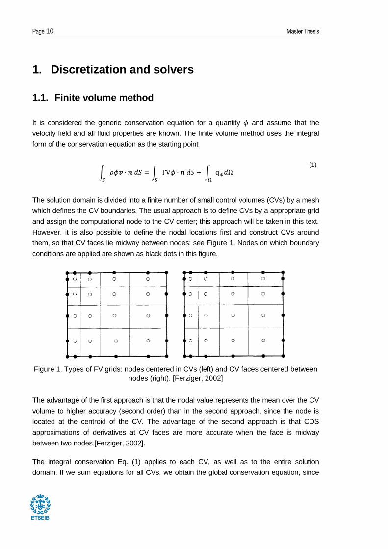
The solution domain is divided into a finite number of small control volumes (CVs) by a mesh
which defines the CV boundaries. The usual approach is to define CVs by a appropriate grid
and assign the computational node to the CV center; this approach will be taken in this text.
However, it is also possible to define the nodal locations first and construct CVs around
them, so that CV faces lie midway between nodes; see Figure 1. Nodes on which boundary
conditions are applied are shown as black dots in this figure.
Figure 1. Types of FV grids: nodes centered in CVs (left) and CV faces centered between
nodes (right). [Ferziger, 2002]
The advantage of the first approach is that the nodal value represents the mean over the CV
volume to higher accuracy (second order) than in the second approach, since the node is
located at the centroid of the CV. The advantage of the second approach is that CDS
approximations of derivatives at CV faces are more accurate when the face is midway
between two nodes [Ferziger, 2002].
The integral conservation Eq. (1) applies to each CV, as well as to the entire solution
domain. If we sum equations for all CVs, we obtain the global conservation equation, since
Numerical methods in heat transfer and fluid dynamics Page 11
surface integrals over inner CV faces cancel out each other. Accordingly, global conservation
is built into the method and this provides one of its principal advantages.
1.1.1. Approximation to surface integrals
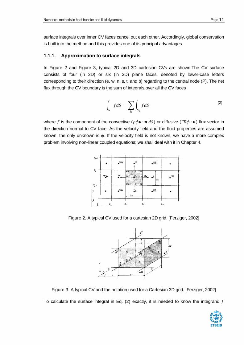
In Figure 2 and Figure 3, typical 2D and 3D cartesian CVs are shown.The CV surface
consists of four (in 2D) or six (in 3D) plane faces, denoted by lower-case letters
corresponding to their direction (e, w, n, s, t, and b) regarding to the central node (P). The net
flux through the CV boundary is the sum of integrals over all the CV faces
(2)
where is the component of the convective or diffusive flux vector in
the direction normal to CV face. As the velocity field and the fluid properties are assumed
known, the only unknown is . If the velocity field is not known, we have a more complex
problem involving non-linear coupled equations; we shall deal with it in Chapter 4.
Figure 2. A typical CV used for a cartesian 2D grid. [Ferziger, 2002]
Figure 3. A typical CV and the notation used for a Cartesian 3D grid. [Ferziger, 2002]
To calculate the surface integral in Eq. (2) exactly, it is needed to know the integrand
Page 12 Master Thesis
everywhere on the surface S. This information is not available, as only the nodal (CV center)
values of are calculated so an approximation must be introduced. This is best done using
two levels of approximation:
the integral is approximated in terms of the variable values at one or more locations
on the cell face
the cell-face values are approximated in terms of the nodal (CV center) values.
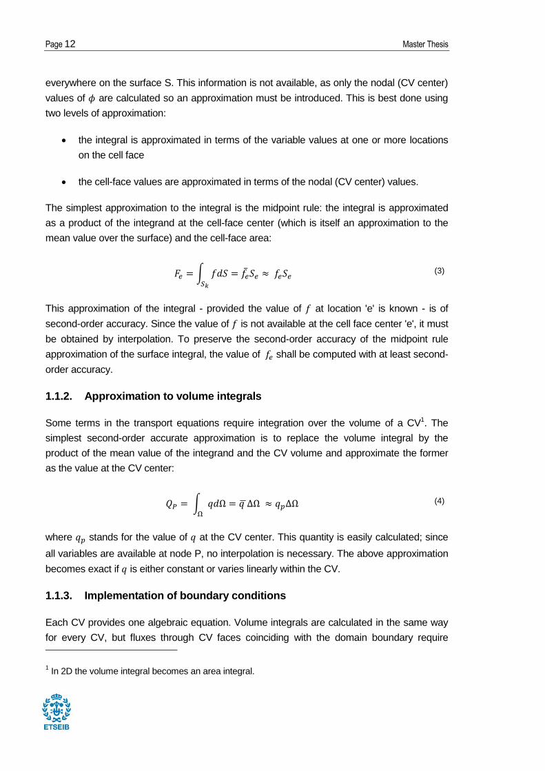
The simplest approximation to the integral is the midpoint rule: the integral is approximated
as a product of the integrand at the cell-face center (which is itself an approximation to the
mean value over the surface) and the cell-face area:
(3)
This approximation of the integral - provided the value of at location 'e' is known - is of
second-order accuracy. Since the value of is not available at the cell face center 'e', it must
be obtained by interpolation. To preserve the second-order accuracy of the midpoint rule
approximation of the surface integral, the value of shall be computed with at least second-
order accuracy.
1.1.2. Approximation to volume integrals
Some terms in the transport equations require integration over the volume of a CV1. The
simplest second-order accurate approximation is to replace the volume integral by the
product of the mean value of the integrand and the CV volume and approximate the former
as the value at the CV center:
(4)
where stands for the value of at the CV center. This quantity is easily calculated; since
all variables are available at node P, no interpolation is necessary. The above approximation
becomes exact if is either constant or varies linearly within the CV.
1.1.3. Implementation of boundary conditions
Each CV provides one algebraic equation. Volume integrals are calculated in the same way
for every CV, but fluxes through CV faces coinciding with the domain boundary require
1 In 2D the volume integral becomes an area integral.
Numerical methods in heat transfer and fluid dynamics Page 13
special treatment. These boundary fluxes must either be known, or be expressed as a
combination of interior values and boundary data. Since they do not give additional
equations, they should not introduce additional unknowns. Since there are no nodes outside
the boundary, these approximations must be based on one-sided differences or
extrapolations.
1.1.4. The algebraic equation system
By summing all the flux approximations and source terms, we produce an algebraic equation
which relates the variable value at the center of the CV to the values at several neighbor
CVs. The numbers of equations and unknowns are both equal to the number of CVs.
1.2. Solution of Linear Equation Systems
It should be noted that, while constructing the discretization equations, we mold them into a
linear form but do not assume a specific method would be used for their solution. Therefore,
any suitable solution method can be employed at this stage. It is useful to consider the
derivation of the equations and their solution as two distinct operations, and there is no need
that one influences the other.
1.2.1. Gauss-Seidel method
The simplest of all iterative methods is the Gauss-Seidel method (GS) in which the values of
the variable are calculated by visiting each grid point in a certain order. The property used
next to explain this method is the temperature; nevertheless, it can be replaced to its general
form with the property .
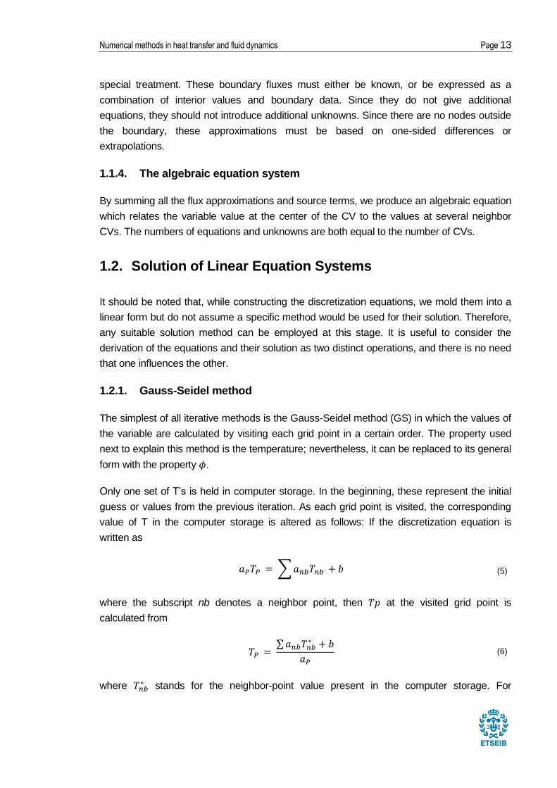
Only one set of T’s is held in computer storage. In the beginning, these represent the initial
guess or values from the previous iteration. As each grid point is visited, the corresponding
value of T in the computer storage is altered as follows: If the discretization equation is
written as
(5)
where the subscript nb denotes a neighbor point, then at the visited grid point is
calculated from
(6)
where stands for the neighbor-point value present in the computer storage. For
Page 14 Master Thesis
neighbors that have already been visited during the current iteration, is the recently
calculated value; for yet-to-be visited neighbors is the value from the previous iteration. In
any case, is the latest available value for the neighbor-point temperature. When all grid
points have been visited in this way, one iteration of the GS is complete.
1.2.2. Tri-diagonal matrix algorithm
The solution of the discretization equations for the one-dimensional situation can be obtained
by the standard Gaussian-elimination method. Because of the particularly simple form of the
equations, the elimination process turns into a convenient algorithm. This is TDMA (Tri-
Diagonal Matrix Algorithm). The designation TDMA refers to the fact that when the matrix of
the coefficients of these equations is written, all the non-zero coefficients align themselves
along three diagonals of the matrix.
Suppose that mesh points are numbered 1, 2, 3, …, N, with points 1 and N denoting the
boundary points. The discretization equations can be written as
(7)
For i = 1, 2, 3, …, N. Thus, the temperature is related to the neighboring temperature
and . To account for the special form of the boundary-point equations, let us set
and (8)
So that the temperatures and will not have any meaningful role to play. These
conditions imply that is known in terms of . The equation for is a relation between
, , and . But, since can be expressed in terms of , this relation reduces to a
relation between and . In other words, can be expressed in terms of . This process
of substitution can be continued until is formally expressed in terms of . But because
has no meaningful existence, we actually obtain the numerical value of at this stage.
This enables us to begin the “back-substituion” process in which is obtained from ,
from , …, from , and from . This is the essence of the TDMA.
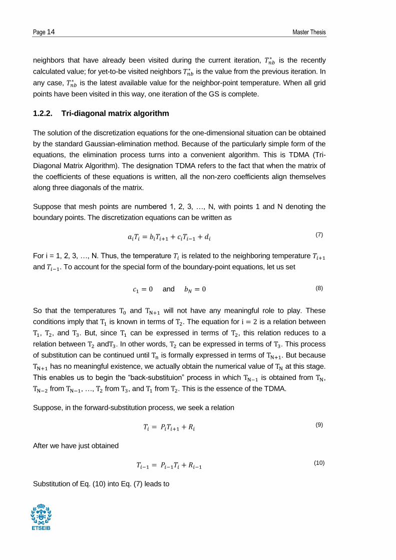
Suppose, in the forward-substitution process, we seek a relation
(9)
After we have just obtained
(10)
Substitution of Eq. (10) into Eq. (7) leads to
Numerical methods in heat transfer and fluid dynamics Page 15
(11)
Which can be rearranged to look like Eq (9). In other words, the coefficients and then
stand for
(12)
(13)
These are recurrence relations, since they give and in terms of and . To start
the recurrence process, we note that Eq. (7) for is almost of the form Eq. (9). Thus, the
values of and are given by
and
(14)
At the other end of the , sequence, we note that . This leads to , and
hence from Eq. (9) it is obtained
(15)
Now we start the back substituion via Eq. (9). The algorithm results
1. Calculate and from Eq. (14)
2. Use the recurrence relations (13) to obtain and for i = 2,3, …, N.
3. Set
4. Use Eq. (9) for , to obtain , , …, , , .
1.2.3. Line-by-line method
A suitable combination of the TDMA for one-dimensional situations and the GS can now be
formed. We shall choose a grid line (say, in the y direction), assume that the temperatures
(or the property of interest) along the neighboring lines (i.e., the x- and z-direction neighbors
of the points on the chosen line) are known from their most-recent values, and solve for the
temperatures (or the property of interest) along the chosen line by the TDMA. We shall follow
this procedure for all the lines in one direction and repeat the procedure, if desired, for the
Page 16 Master Thesis
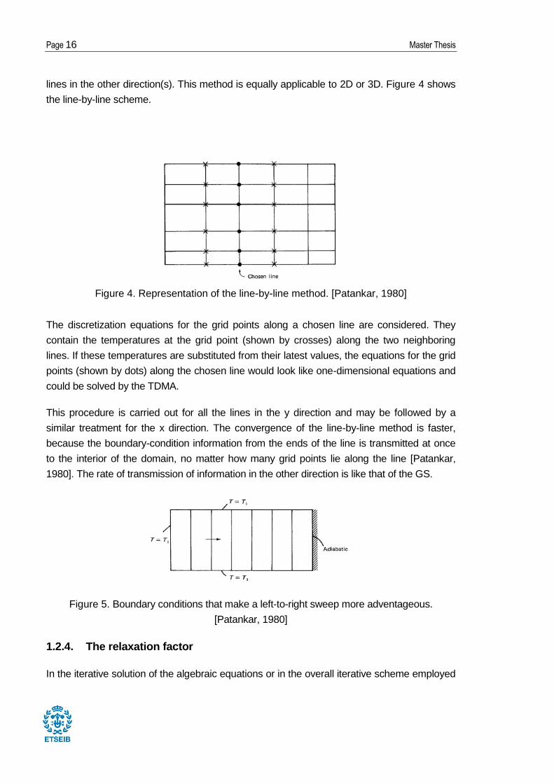
lines in the other direction(s). This method is equally applicable to 2D or 3D. Figure 4 shows
the line-by-line scheme.
Figure 4. Representation of the line-by-line method. [Patankar, 1980]
The discretization equations for the grid points along a chosen line are considered. They
contain the temperatures at the grid point (shown by crosses) along the two neighboring
lines. If these temperatures are substituted from their latest values, the equations for the grid
points (shown by dots) along the chosen line would look like one-dimensional equations and
could be solved by the TDMA.
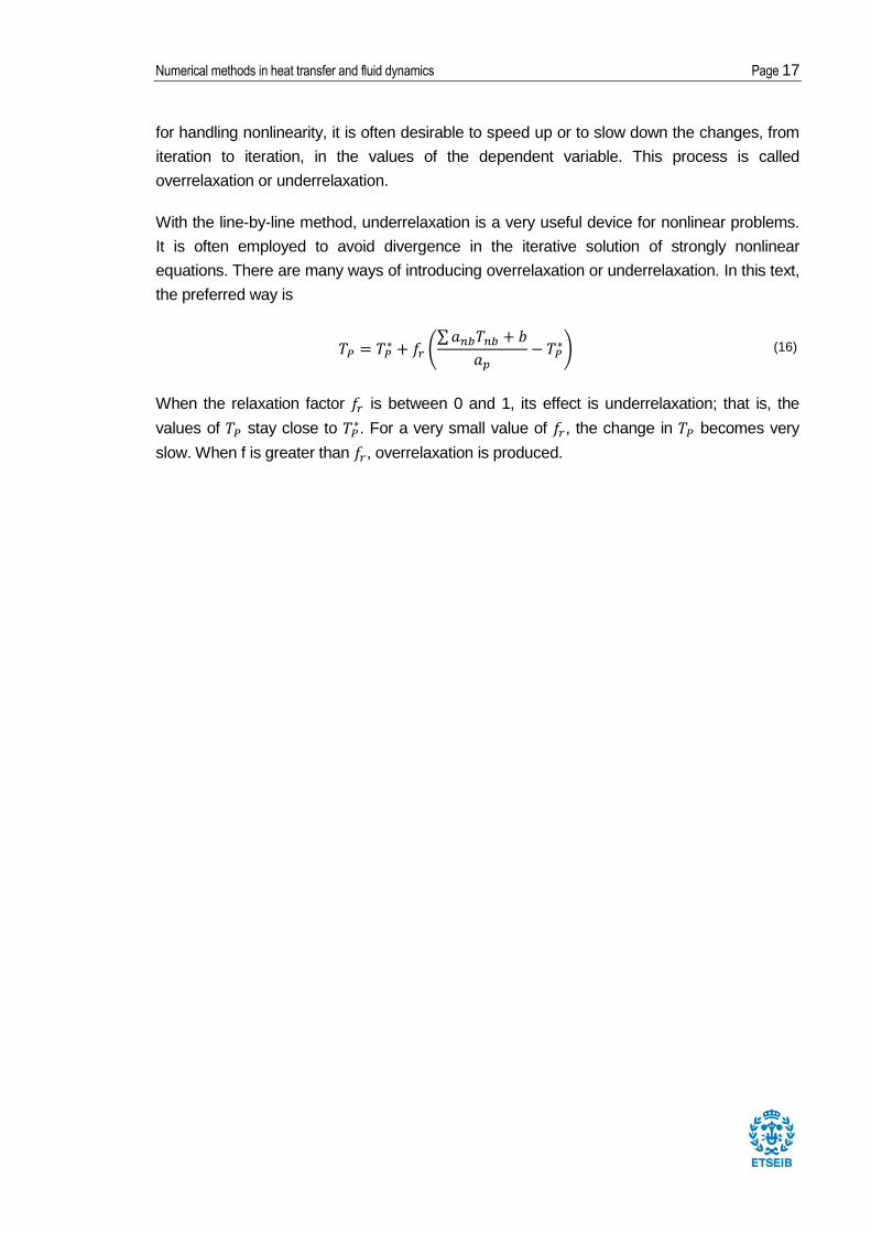
This procedure is carried out for all the lines in the y direction and may be followed by a
similar treatment for the x direction. The convergence of the line-by-line method is faster,
because the boundary-condition information from the ends of the line is transmitted at once
to the interior of the domain, no matter how many grid points lie along the line [Patankar,
1980]. The rate of transmission of information in the other direction is like that of the GS.
Figure 5. Boundary conditions that make a left-to-right sweep more adventageous.
[Patankar, 1980]
1.2.4. The relaxation factor
In the iterative solution of the algebraic equations or in the overall iterative scheme employed
Numerical methods in heat transfer and fluid dynamics Page 17
for handling nonlinearity, it is often desirable to speed up or to slow down the changes, from
iteration to iteration, in the values of the dependent variable. This process is called
overrelaxation or underrelaxation.
With the line-by-line method, underrelaxation is a very useful device for nonlinear problems.
It is often employed to avoid divergence in the iterative solution of strongly nonlinear
equations. There are many ways of introducing overrelaxation or underrelaxation. In this text,
the preferred way is
(16)
When the relaxation factor is between 0 and 1, its effect is underrelaxation; that is, the
values of stay close to . For a very small value of , the change in becomes very
slow. When f is greater than , overrelaxation is produced.
Page 18 Master Thesis
2. Heat conduction methods
In this chapter, we shall begin the task of constructing a numerical method for solving the
general differential equation (17), which governs the physical process of interest here.
(17)
This equation contains four basic terms. Here we shall omit the convection term (the second
term) and concentrate on the remaining three terms. The construction of the method will be
completed in Chapter 3, where the treatment of the convection term will be discussed.
Omission of the convection term reduces the situation to a conduction-type problem. Heat
conduction provides a convenient starting point for our formulation, because the physical
processes are easy to understand and the mathematical complication is minimal.
The objectives of this chapter, however, go far beyond presenting a numerical method for
heat conduction alone. First, other physical processes are governed by very similar
mathematical equations. Among these are potential flow, mass diffusion, flow through porous
media, and some fully developed duct flows. The numerical techniques described in this
chapter are directly applicable to all these processes. Electromagnetic field theory, diffusion
models of thermal radiation, and lubrication flows are further examples of phenomena
governed by conduction-type equations.
Second, this chapter accomplishes much of the preparatory work needed for later chapters.
The procedure for the solution of the algebraic equations is presented here in a once-and-
for-all manner. Later chapters modify the content of the algebraic equations, but the same
solution technique continues to be applicable.
2.1. Heat conduction discretized equation
A portion of a 2D grid is shown in Figure 6. For the grid point P (denoting principal), points E
and W (denoting east and west) are its x-direction neighbors, while N and S (denoting north
and south) are the y-direction neighbors. The CV around P is shown dashed by lines. Its
thickness in the z-direction is assumed to be unity. The HT surfaces are indicated with a
lowercase letter.
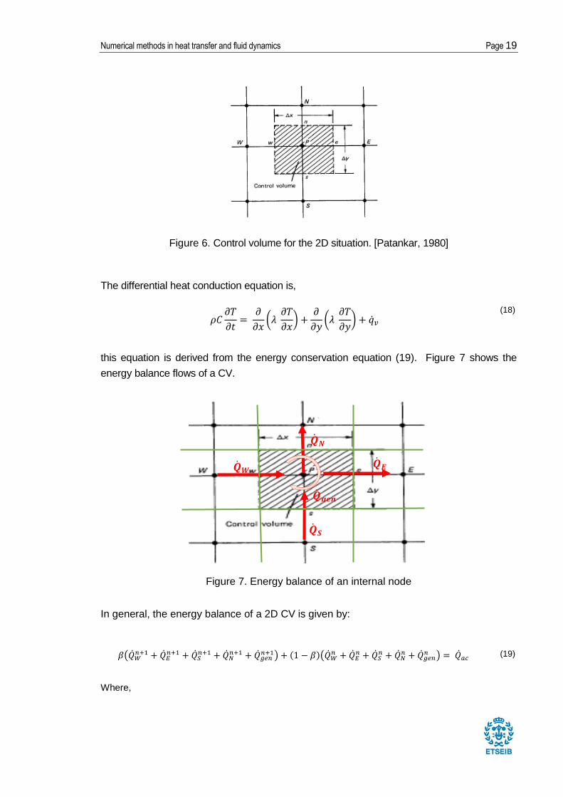
Numerical methods in heat transfer and fluid dynamics Page 19
Figure 6. Control volume for the 2D situation. [Patankar, 1980]
The differential heat conduction equation is,
(18)
this equation is derived from the energy conservation equation (19). Figure 7 shows the
energy balance flows of a CV.
Figure 7. Energy balance of an internal node
In general, the energy balance of a 2D CV is given by:
(19)
Where,
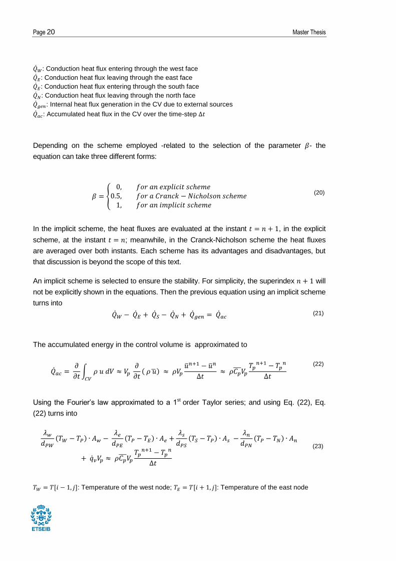
Page 20 Master Thesis
: Conduction heat flux entering through the west face
: Conduction heat flux leaving through the east face
: Conduction heat flux entering through the south face
: Conduction heat flux leaving through the north face
: Internal heat flux generation in the CV due to external sources
: Accumulated heat flux in the CV over the time-step
Depending on the scheme employed -related to the selection of the parameter - the
equation can take three different forms:
(20)
In the implicit scheme, the heat fluxes are evaluated at the instant , in the explicit
scheme, at the instant ; meanwhile, in the Cranck-Nicholson scheme the heat fluxes
are averaged over both instants. Each scheme has its advantages and disadvantages, but
that discussion is beyond the scope of this text.
An implicit scheme is selected to ensure the stability. For simplicity, the superindex will
not be explicitly shown in the equations. Then the previous equation using an implicit scheme
turns into
(21)
The accumulated energy in the control volume is approximated to
(22)
Using the Fourier’s law approximated to a 1st order Taylor series; and using Eq. (22), Eq.
(22) turns into
(23)
: Temperature of the west node; : Temperature of the east node
Numerical methods in heat transfer and fluid dynamics Page 21
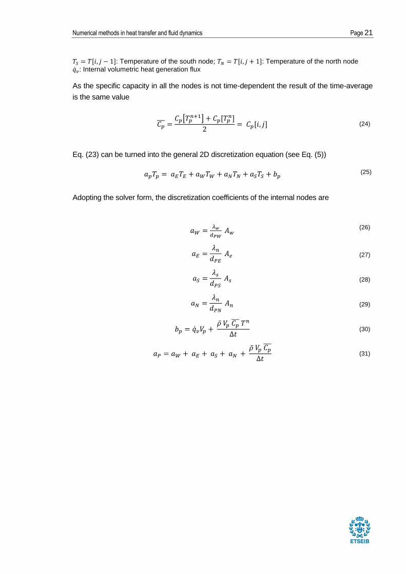
: Temperature of the south node; : Temperature of the north node
: Internal volumetric heat generation flux
As the specific capacity in all the nodes is not time-dependent the result of the time-average
is the same value
(24)
Eq. (23) can be turned into the general 2D discretization equation (see Eq. (5))
(25)
Adopting the solver form, the discretization coefficients of the internal nodes are
(26)
(27)
(28)
(29)
(30)
(31)
Page 22 Master Thesis
2.2. The Four materials problem
The Four materials problem is a benchmark heat conduction problem in transient regime
problem proposed by the CTTC (2016). The name ‘four materials’ is because the problem is
modeled as a rod composed by four different materials, each one with its own
thermophysical properties and size. The problem is defined, solved, verified and validated
next.
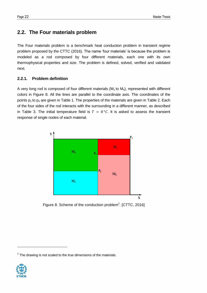
2.2.1. Problem definition
A very long rod is composed of four different materials (M1 to M4), represented with different
colors in Figure 8. All the lines are parallel to the coordinate axis. The coordinates of the
points p1 to p3 are given in Table 1. The properties of the materials are given in Table 2. Each
of the four sides of the rod interacts with the surrounding in a different manner, as described
in Table 3. The initial temperature field is It is asked to assess the transient
response of single nodes of each material.
Figure 8. Scheme of the conduction problem2. [CTTC, 2016]
2 The drawing is not scaled to the true dimensions of the materials.
Numerical methods in heat transfer and fluid dynamics Page 23
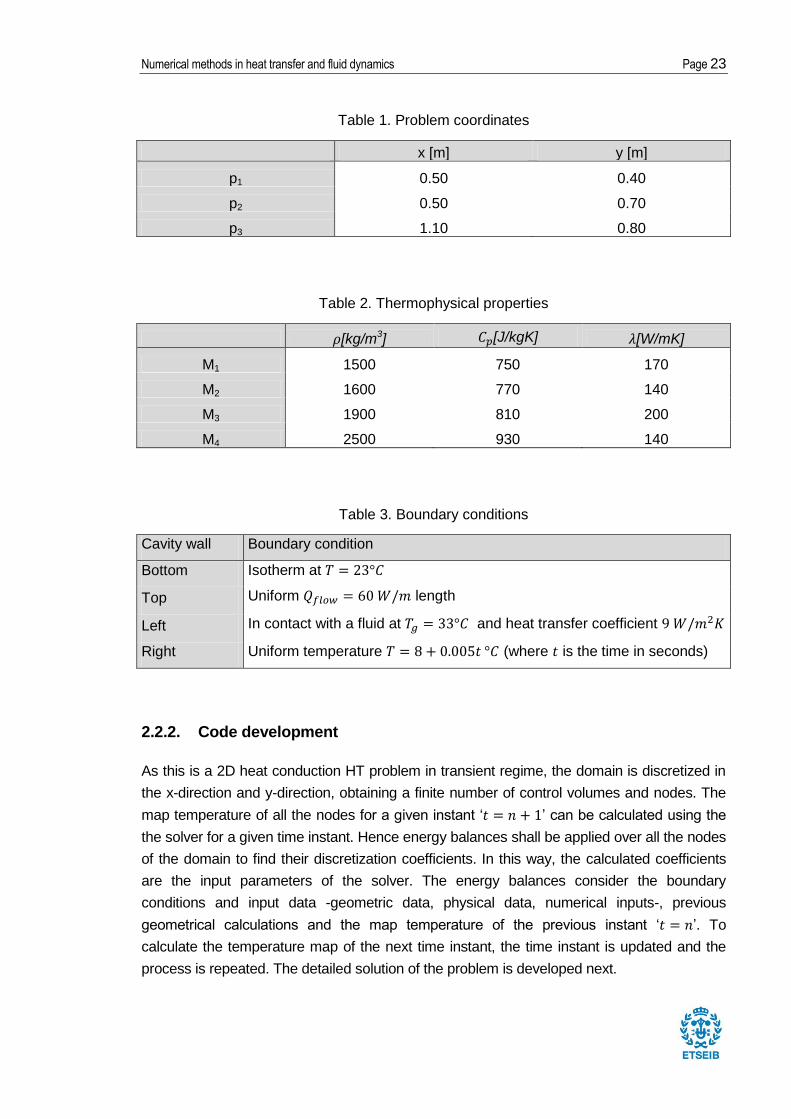
Table 1. Problem coordinates
x [m] y [m]
p1 0.50 0.40
p2 0.50 0.70
p3 1.10 0.80
Table 2. Thermophysical properties
[kg/m3] [J/kgK] [W/mK]
M1 1500 750 170
M2 1600 770 140
M3 1900 810 200
M4 2500 930 140
Table 3. Boundary conditions
Cavity wall Boundary condition
Bottom Isotherm at
Top Uniform length
Left In contact with a fluid at and heat transfer coefficient
Right Uniform temperature (where is the time in seconds)
2.2.2. Code development
As this is a 2D heat conduction HT problem in transient regime, the domain is discretized in
the x-direction and y-direction, obtaining a finite number of control volumes and nodes. The
map temperature of all the nodes for a given instant ‘ ’ can be calculated using the
the solver for a given time instant. Hence energy balances shall be applied over all the nodes
of the domain to find their discretization coefficients. In this way, the calculated coefficients
are the input parameters of the solver. The energy balances consider the boundary
conditions and input data -geometric data, physical data, numerical inputs-, previous
geometrical calculations and the map temperature of the previous instant ‘ ’. To
calculate the temperature map of the next time instant, the time instant is updated and the
process is repeated. The detailed solution of the problem is developed next.
Page 24 Master Thesis
Assumptions
Two-dimensional flow – x-axis and y-axis–, z-axis flow is neglected.
Constant thermophysical properties –density, thermal conductivity, specific
capacity– for each material.
HT phenomena: only conduction within the solid, conduction and convection in the
left-side and top-side.
Cell-centered discretization: average values over each cell –temperature, density,
specific capacity, thermal conductivity–.
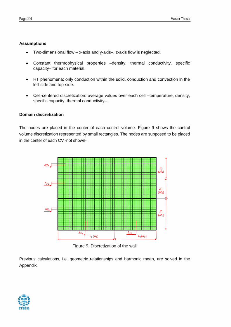
Domain discretization
The nodes are placed in the center of each control volume. Figure 9 shows the control
volume discretization represented by small rectangles. The nodes are supposed to be placed
in the center of each CV -not shown-.
Figure 9. Discretization of the wall
Previous calculations, i.e. geometric relationships and harmonic mean, are solved in the
Appendix.
Numerical methods in heat transfer and fluid dynamics Page 25
Discretization coefficients
The discretization coefficients of the internal nodes are the ones obtained from the procedure
of Section 2.1. This procedure is analogously followed to obtain the discretization coefficients
of the nodes located in the left side, top side, right side and bottom side.
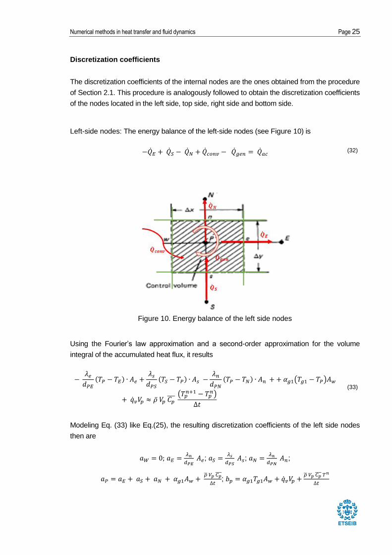
Left-side nodes: The energy balance of the left-side nodes (see Figure 10) is
(32)
Figure 10. Energy balance of the left side nodes
Using the Fourier’s law approximation and a second-order approximation for the volume
integral of the accumulated heat flux, it results
(33)
Modeling Eq. (33) like Eq.(25), the resulting discretization coefficients of the left side nodes
then are
;
;
;
;
Page 26 Master Thesis
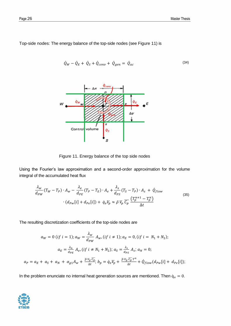
Top-side nodes: The energy balance of the top-side nodes (see Figure 11) is
(34)
Figure 11. Energy balance of the top side nodes
Using the Fourier’s law approximation and a second-order approximation for the volume
integral of the accumulated heat flux
(35)
The resulting discretization coefficients of the top-side nodes are
;
;
;
;
In the problem enunciate no internal heat generation sources are mentioned. Then .
Numerical methods in heat transfer and fluid dynamics Page 27
Right-side nodes: The temperature of the right-side nodes is uniform and is given by
.
;
Bottom-side nodes: These nodes shape an isotherm .
;
As physical properties are time-independent3, is the only time-dependent coefficient.
Solver
The GS for 2D or line-by-line method can be used. The equation required for the line by line
method, TDMA for solving horizontal lines with vertical sweeping direction, is
where
(36) (37)
After obtaining all the discretization coefficients, the temperature map is obtained using the
line-by-line method. In this case, the parameters and are calculated as follows
employing the TDMA as many times as rows has the domain, this is for
.
For i = 1
3 are constant throughout the time and may be calculated out of the time loop if
desired, although this may not be considered a good practice.
Page 28 Master Thesis
For i > 1
Afterwards, the temperature map is calculated “line-by-line” for ,
employing the calculated parameters P and R.
For i = N1 + N2:
For i = N1+ N2 - 1 to 1
2.2.3. Algorithm
The algorithm proposal for the resolution of the Four materials problem is presented below.
1. Input data:
Physical data:
Numerical data: , .4
Geometrical data:
Boundary conditions: .
2. Previous calculations: . These
variables are calculated using only the input data. See Annex A.
3. The initial map is given: .
4 The number of nodes N, M, the convergence criteria, δ and the time-step Δt must be carefully and
correctly selected, otherwise they may influence in the results, which are supposed to be
independent of these parameters.
Numerical methods in heat transfer and fluid dynamics Page 29
4. Update the time instant: . Propose a temperature map for instant:
.5 e.g. the temperature map of the instant :´
5. Calculation of the temperature map :
5.1 Calculate the discretization coefficients of all the nodes.
5.2 Calculate the temperature map using the line-by-line or GS solver, using
the last calculated temperatures whenever possible.
5.3 Apply the convergence criteria: Is ,
If no: . (Refresh the guessed temperature map to the last
calculated values); and go to 5.1.
If yes: If wanted, save the temperature map . Go to 6.
6. Is (Evaluation of the last instant).
If no: Go to 4
If yes: Go to 7.
7. Final calculations and print results.
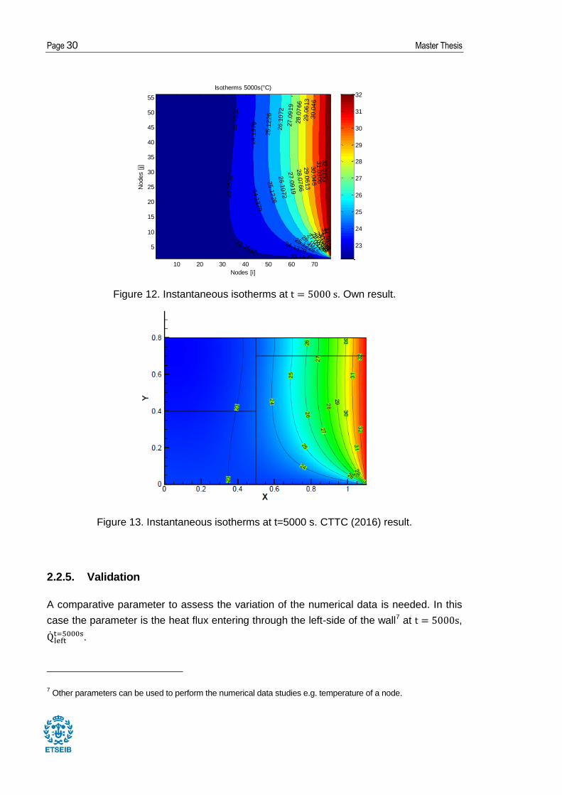
2.2.4. Verification
The numerical data used to solve the problem are: a node density6 of ,
convergence criterion and a time-step =1 s. The isotherms at t = 5000 s are
shown in Figure 12. This result matches with the CTTC result shown in Figure 13.
5 Note that strictly the denomination is only correct when . In general, the correct
denomination is , but for simplicity here is used.
6 The number of nodes is obtained multiplying the node density per a length. In the case of our domain:
Page 30 Master Thesis
Figure 12. Instantaneous isotherms at . Own result.
Figure 13. Instantaneous isotherms at t=5000 s. CTTC (2016) result.
2.2.5. Validation
A comparative parameter to assess the variation of the numerical data is needed. In this
case the parameter is the heat flux entering through the left-side of the wall7 at ,
.
7 Other parameters can be used to perform the numerical data studies e.g. temperature of a node.
23.1532
23.1532
23
.15
32
23
.15
32
24.1379
24
.13
79
24
.13
79
25.1226
25
.12
26
25
.12
26
26.1072
26
.10
72
26
.10
72
27.0919
27
.09
19
27
.09
19
28.07
66
28
.07
66
28
.07
66
29.0
613
29
.06
13
29
.06
13
30
.04
6
30
.04
6
30
.04
6
31
.03
06
31
.03
06
32
.01
53
32.0
153
Nodes [
j]
Nodes [i]
Isotherms 5000s(°C)
10 20 30 40 50 60 70
5
10
15
20
25
30
35
40
45
50
55
23
24
25
26
27
28
29
30
31
32
Numerical methods in heat transfer and fluid dynamics Page 31
(38)
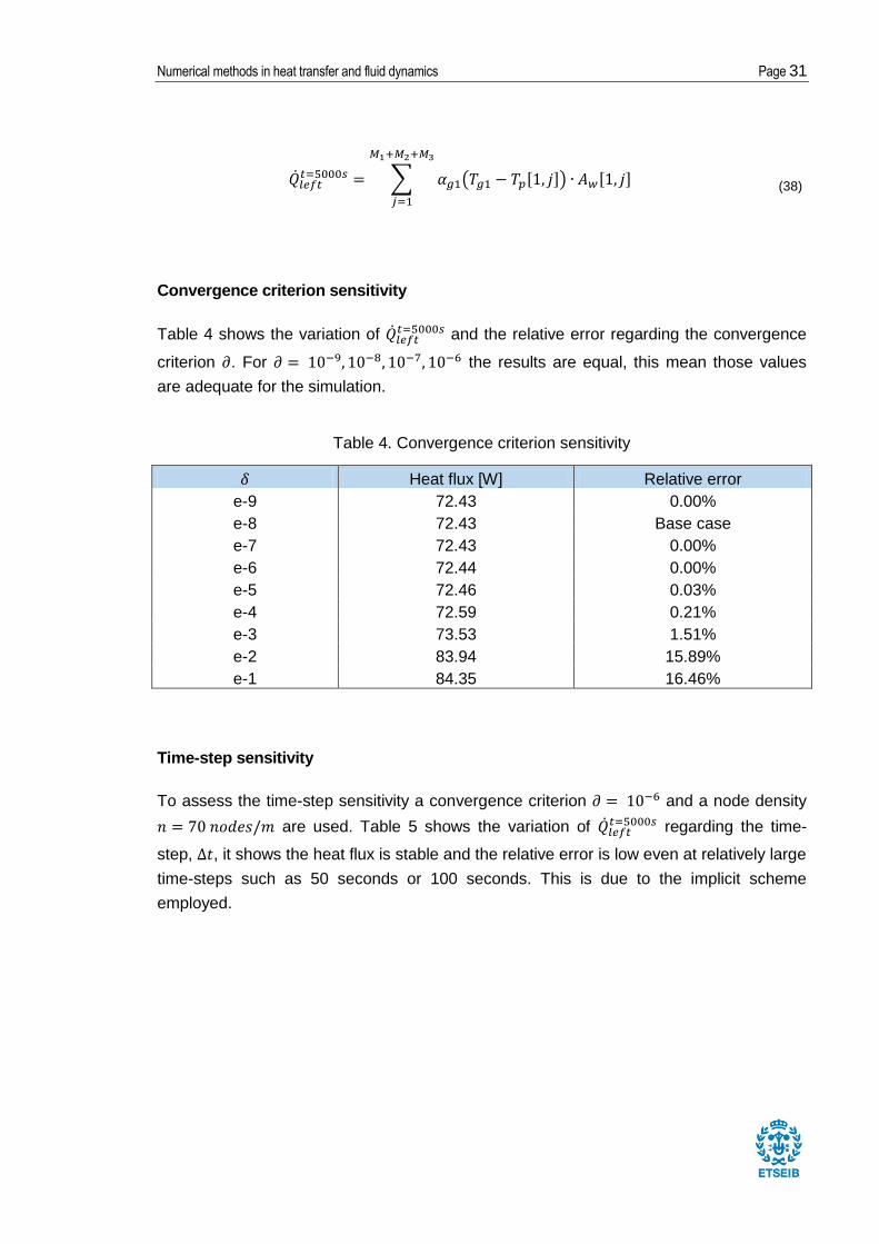
Convergence criterion sensitivity
Table 4 shows the variation of and the relative error regarding the convergence
criterion . For the results are equal, this mean those values
are adequate for the simulation.
Table 4. Convergence criterion sensitivity
Heat flux [W] Relative error
e-9 72.43 0.00%
e-8 72.43 Base case
e-7 72.43 0.00%
e-6 72.44 0.00%
e-5 72.46 0.03%
e-4 72.59 0.21%
e-3 73.53 1.51%
e-2 83.94 15.89%
e-1 84.35 16.46%
Time-step sensitivity
To assess the time-step sensitivity a convergence criterion and a node density
are used. Table 5 shows the variation of regarding the time-
step, , it shows the heat flux is stable and the relative error is low even at relatively large
time-steps such as 50 seconds or 100 seconds. This is due to the implicit scheme
employed.
Page 32 Master Thesis
Table 5. Time-step sensitivity
∆t Heat flux [W] Relative error
1 73.05 Base case
2 73.05 0.00%
5 73.06 0.01%
10 73.07 0.03%
20 73.09 0.06%
25 73.10 0.07%
50 73.15 0.14%
100 73.26 0.29%
200 73.47 0.58%
250 73.58 0.72%
500 74.12 1.47%
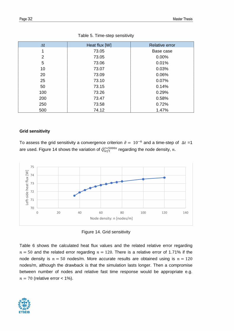
Grid sensitivity
To assess the grid sensitivity a convergence criterion and a time-step of =1
are used. Figure 14 shows the variation of regarding the node density, .
Figure 14. Grid sensitivity
Table 6 shows the calculated heat flux values and the related relative error regarding
and the related error regarding There is a relative error of 1.71% if the
node density is nodes/m. More accurate results are obtained using is
nodes/m, although the drawback is that the simulation lasts longer. Then a compromise
between number of nodes and relative fast time response would be appropriate e.g.
(relative error < 1%).
70
71
72
73
74
75
0 20 40 60 80 100 120 140
Left
-sid
e h
eat
flu
x [W
]
Node density: n [nodes/m]
Numerical methods in heat transfer and fluid dynamics Page 33
Table 6. Grid sensitivity
Node density
Heat flux [W]
Relative error
Relative error
120 73.70 1.74% Base case
100 73.51 1.49% 0.25%
80 73.24 1.11% 0.62%
75 73.15 0.98% 0.75%
70 73.05 0.85% 0.88%
65 72.92 0.67% 1.05%
60 72.79 0.49% 1.23%
55 72.62 0.26% 1.46%
50 72.44 Base case 1.71%
45 72.19 0.34% 2.05%
40 71.90 0.74% 2.44%
35 71.50 1.29% 2.98%
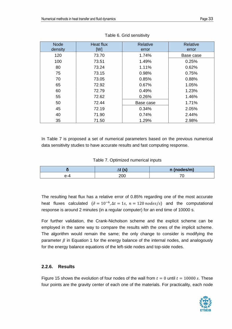
In Table 7 is proposed a set of numerical parameters based on the previous numerical
data sensitivity studies to have accurate results and fast computing response.
Table 7. Optimized numerical inputs
δ ∆t (s) n (nodes/m)
e-4 200 70
The resulting heat flux has a relative error of 0.85% regarding one of the most accurate
heat fluxes calculated ( ) and the computational
response is around 2 minutes (in a regular computer) for an end time of 10000 s.
For further validation, the Crank-Nicholson scheme and the explicit scheme can be
employed in the same way to compare the results with the ones of the implicit scheme.
The algorithm would remain the same; the only change to consider is modifying the
parameter in Equation 1 for the energy balance of the internal nodes, and analogously
for the energy balance equations of the left-side nodes and top-side nodes.
2.2.6. Results
Figure 15 shows the evolution of four nodes of the wall from until . These
four points are the gravity center of each one of the materials. For practicality, each node
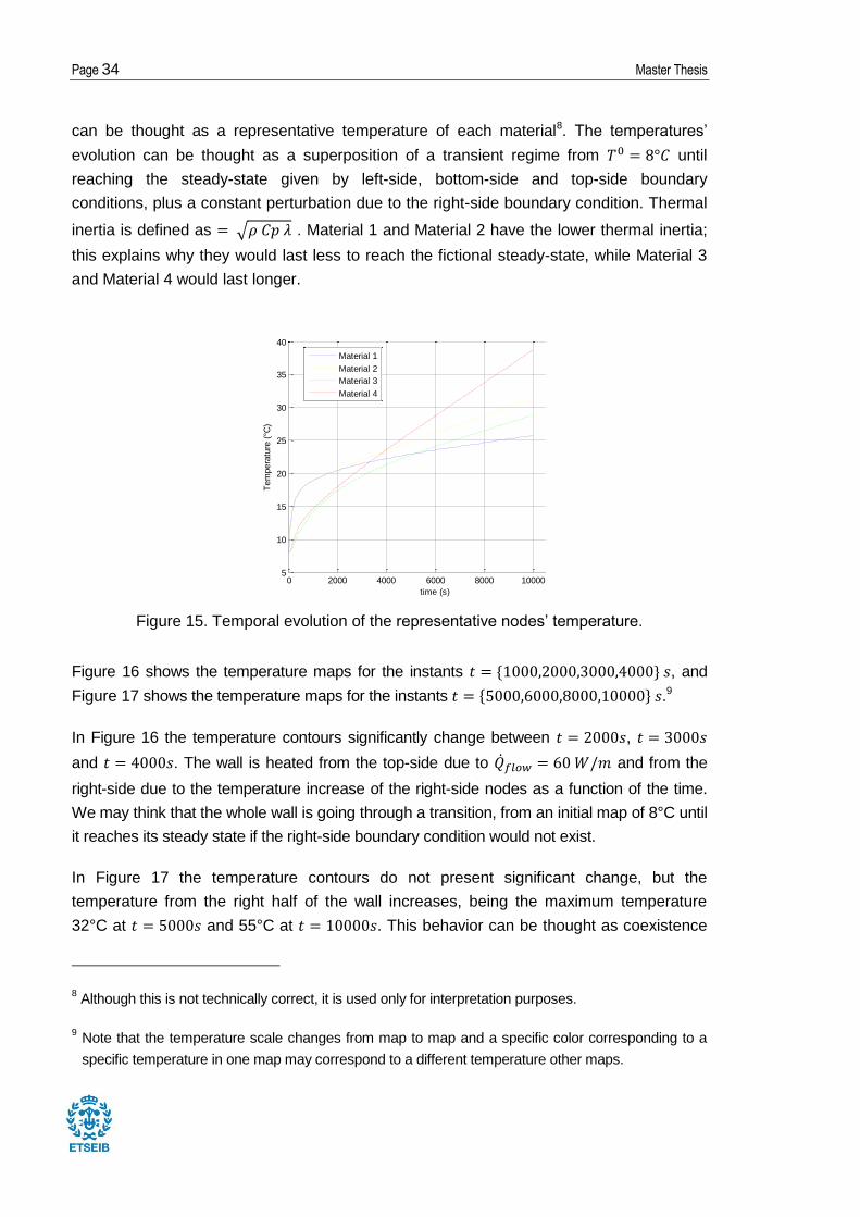
Page 34 Master Thesis
can be thought as a representative temperature of each material8. The temperatures’
evolution can be thought as a superposition of a transient regime from until
reaching the steady-state given by left-side, bottom-side and top-side boundary
conditions, plus a constant perturbation due to the right-side boundary condition. Thermal
inertia is defined as . Material 1 and Material 2 have the lower thermal inertia;
this explains why they would last less to reach the fictional steady-state, while Material 3
and Material 4 would last longer.
Figure 15. Temporal evolution of the representative nodes’ temperature.
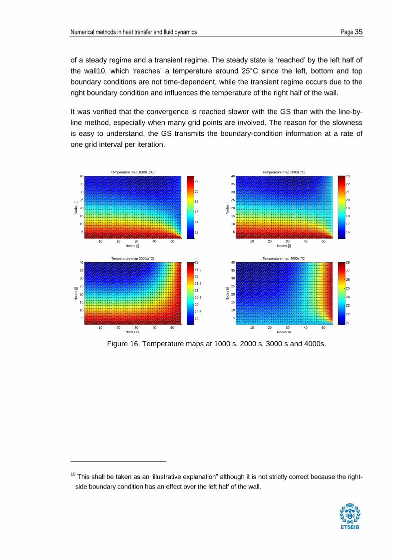
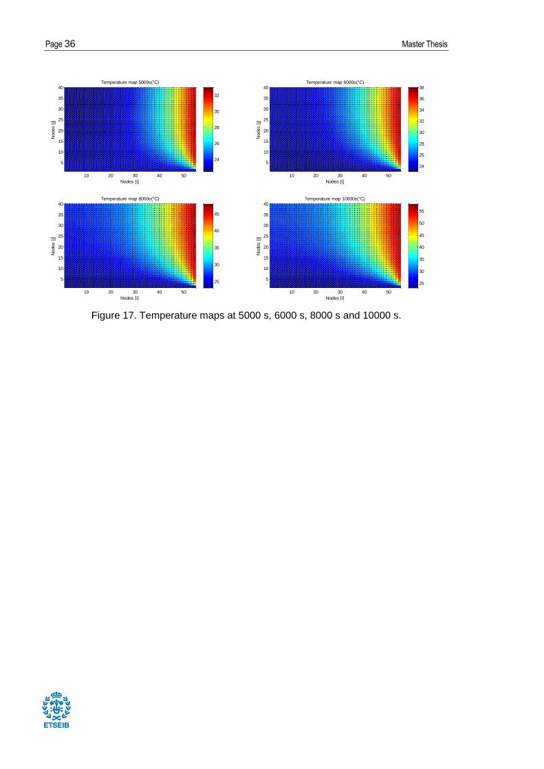
Figure 16 shows the temperature maps for the instants , and
Figure 17 shows the temperature maps for the instants .9
In Figure 16 the temperature contours significantly change between ,
and . The wall is heated from the top-side due to and from the
right-side due to the temperature increase of the right-side nodes as a function of the time.
We may think that the whole wall is going through a transition, from an initial map of 8°C until
it reaches its steady state if the right-side boundary condition would not exist.
In Figure 17 the temperature contours do not present significant change, but the
temperature from the right half of the wall increases, being the maximum temperature
32°C at and 55°C at . This behavior can be thought as coexistence
8 Although this is not technically correct, it is used only for interpretation purposes.
9 Note that the temperature scale changes from map to map and a specific color corresponding to a
specific temperature in one map may correspond to a different temperature other maps.
0 2000 4000 6000 8000 10000 120005
10
15
20
25
30
35
40
time (s)
Tem
pera
ture
(°C
)
Material 1
Material 2
Material 3
Material 4
Numerical methods in heat transfer and fluid dynamics Page 35
of a steady regime and a transient regime. The steady state is ‘reached’ by the left half of
the wall10, which ‘reaches’ a temperature around 25°C since the left, bottom and top
boundary conditions are not time-dependent, while the transient regime occurs due to the
right boundary condition and influences the temperature of the right half of the wall.
It was verified that the convergence is reached slower with the GS than with the line-by-
line method, especially when many grid points are involved. The reason for the slowness
is easy to understand, the GS transmits the boundary-condition information at a rate of
one grid interval per iteration.
Figure 16. Temperature maps at 1000 s, 2000 s, 3000 s and 4000s.
10 This shall be taken as an ‘illustrative explanation” although it is not strictly correct because the right-
side boundary condition has an effect over the left half of the wall.
10 20 30 40 50
5
10
15
20
25
30
35
40
Nodes [
j]
Nodes [i]
Temperature map 1000s (°C)
10 20 30 40 50
5
10
15
20
25
30
35
40
Nodes [
j]
Nodes [i]
Temperature map 2000s(°C)
10 20 30 40 50
5
10
15
20
25
30
35
40
Nodes [
j]
Nodes [i]
Temperature map 3000s(°C)
10 20 30 40 50
5
10
15
20
25
30
35
40
Nodes [
j]
Nodes [i]
Temperature map 4000s(°C)
12
14
16
18
20
22
16
17
18
19
20
21
22
23
19
19.5
20
20.5
21
21.5
22
22.5
23
21
22
23
24
25
26
27
28
Page 36 Master Thesis
Figure 17. Temperature maps at 5000 s, 6000 s, 8000 s and 10000 s.
10 20 30 40 50
5
10
15
20
25
30
35
40
Nodes [
j]
Nodes [i]
Temperature map 5000s(°C)
10 20 30 40 50
5
10
15
20
25
30
35
40
Nodes [
j]
Nodes [i]
Temperature map 6000s(°C)
10 20 30 40 50
5
10
15
20
25
30
35
40
Nodes [
j]
Nodes [i]
Temperature map 8000s(°C)
10 20 30 40 50
5
10
15
20
25
30
35
40
Nodes [
j]
Nodes [i]
Temperature map 10000s(°C)
25
30
35
40
45
50
55
24
26
28
30
32
24
26
28
30
32
34
36
38
25
30
35
40
45
Numerical methods in heat transfer and fluid dynamics Page 37
3. Analysis of the general convection-diffusion
equation
This chapter shows how the FVM is applied to a model of convective transport: the 2D
convection-diffusion equation. There are two main goals of this chapter; the first is to
expose the FVM, and the second goal is to introduce and compare the numerical
schemes meddling the convective term in transport equations.
The 2D convection-diffusion equation is a compact, though somewhat non-physical,
model of transport of heat, mass and other passive scalars. Applying the FVM to this
equation allows different schemes for approximating the convection term to be compared.
This chapter should be considered a brief introduction to the topic of convection modeling
schemes. The schemes considered are the upwind difference scheme (UDS), the central
difference scheme (CDS), the exponential difference scheme (EDS), the second-order
upwind scheme (SUDS) and the quadratic interpolation for convective kinematics
(QUICK).
3.1. The convection-diffusion equation
The general differential equation is
(39)
where is the diffusion coefficient and the source term. The quantities and are
specific to a particular meaning of . The four terms in the general differential equation
are the unsteady term, the convection term, the diffusion term, and the source term.
The mass conservation equation
can also be written as Eq. (39) where
, , .
Table 8 shows that momentum, energy and species conservation equations can also be
written using the convection-diffusion equation.

Page 38 Master Thesis
Table 8. Conservation equations written with the convection-diffusion form
.
3.1.1. Domain and temporal discretization
The FVM approach is employed to discretize the general convection-diffusion equation.
Structured meshes (centered nodes or centered faces) and unstructured meshes (usually
centered nodes) are employed to model the spatial domain [CTTC, 2017]. Time is
discretized (see
Figure 18) and the time-step has an essential influence over the stability of the solution.
Figure 18. Scheme of the time discretization
3.1.2. Mass conservation equation
The mass conservation equation on its discretized form shall be obtained as a previous
step for discretizing the convection-diffusion equation, in its differential form is
. . . t
t=0 t1 t2 t3 . . . tn tn+1
Numerical methods in heat transfer and fluid dynamics Page 39
(40)
Integrating over the volume and time
(41)
For an easier notation: and . Assuming second-order approximations,
implicit scheme , mass flow at the faces: in the positive
coordinate direction .
(42)
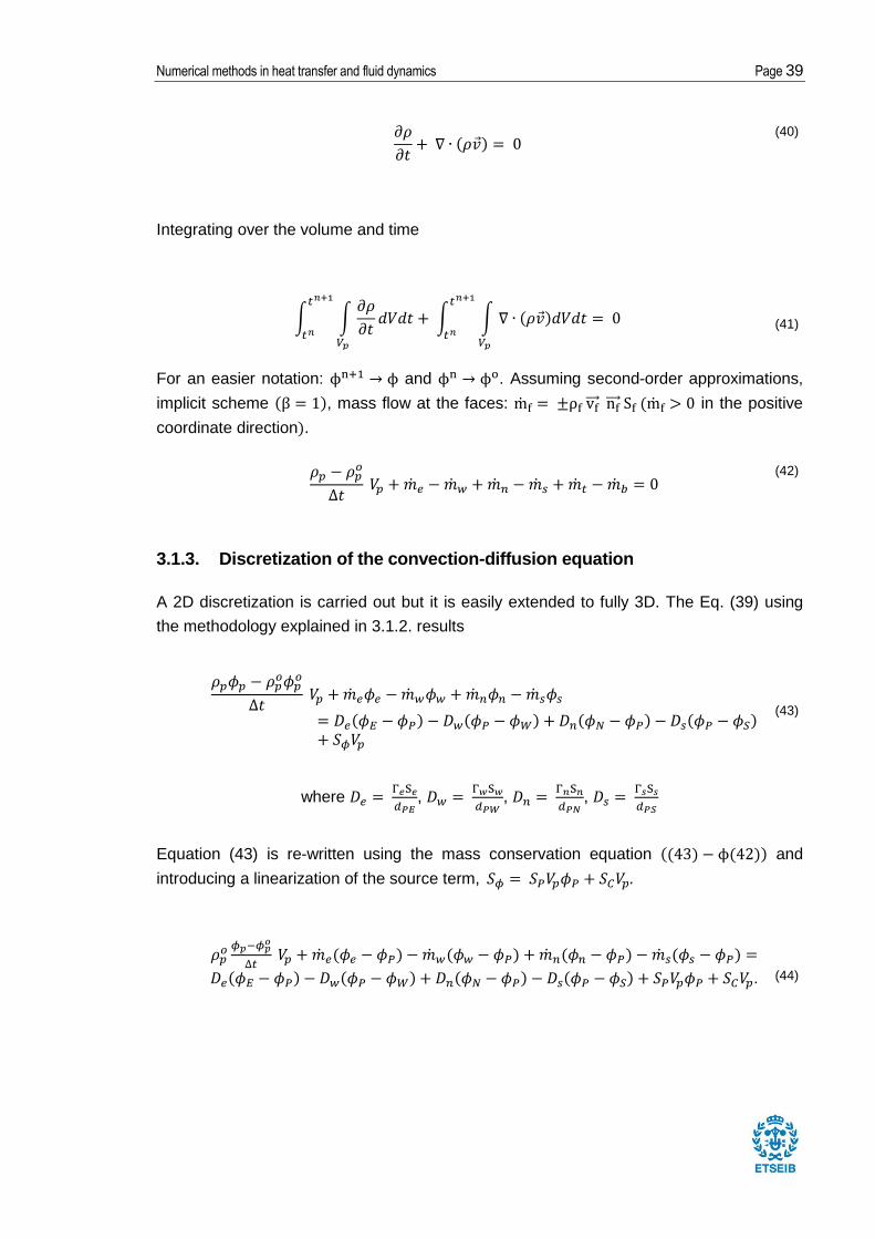
3.1.3. Discretization of the convection-diffusion equation
A 2D discretization is carried out but it is easily extended to fully 3D. The Eq. (39) using
the methodology explained in 3.1.2. results
(43)
where
,
,
,
Equation (43) is re-written using the mass conservation equation and
introducing a linearization of the source term, .
.
(44)
Page 40 Master Thesis
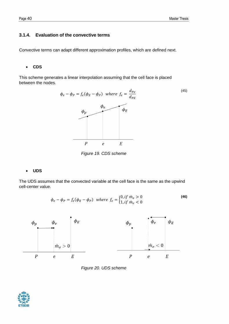
3.1.4. Evaluation of the convective terms
Convective terms can adapt different approximation profiles, which are defined next.
CDS
This scheme generates a linear interpolation assuming that the cell face is placed
between the nodes.
(45)
Figure 19. CDS scheme
UDS
The UDS assumes that the convected variable at the cell face is the same as the upwind
cell-center value.
(46)
Figure 20. UDS scheme
Numerical methods in heat transfer and fluid dynamics Page 41
EDS
The assumed profile between P and E is based on a simplified form of Eq. (39) (steady,
2D, ):
(47)
Assuming
(constant between P and E):
(48)
This equation can be easily integrated from to .
(49)
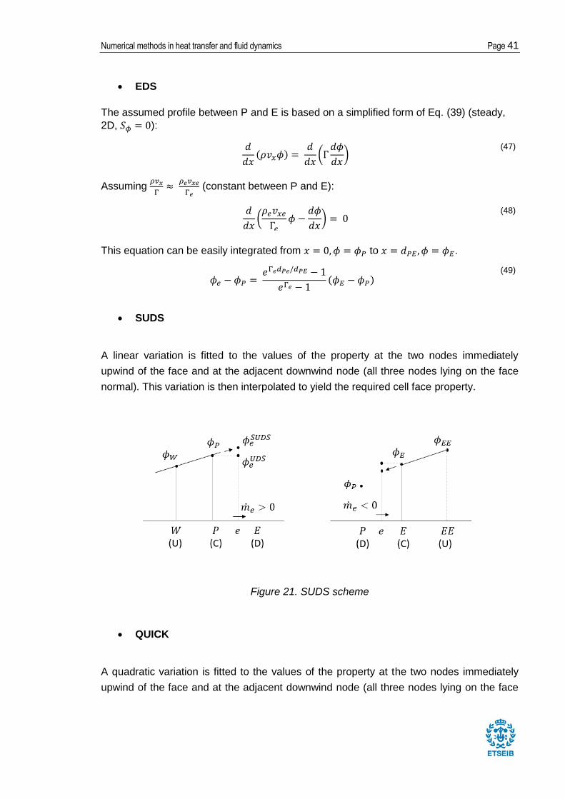
SUDS
A linear variation is fitted to the values of the property at the two nodes immediately
upwind of the face and at the adjacent downwind node (all three nodes lying on the face
normal). This variation is then interpolated to yield the required cell face property.
Figure 21. SUDS scheme
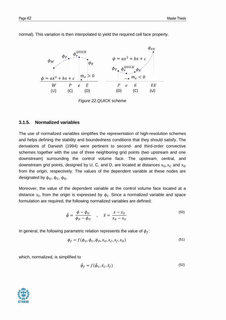
QUICK
A quadratic variation is fitted to the values of the property at the two nodes immediately
upwind of the face and at the adjacent downwind node (all three nodes lying on the face
Page 42 Master Thesis
normal). This variation is then interpolated to yield the required cell face property.
Figure 22.QUICK scheme
3.1.5. Normalized variables
The use of normalized variables simplifies the representation of high-resolution schemes
and helps defining the stability and boundedness conditions that they should satisfy. The
derivations of Darwish (1994) were pertinent to second- and third-order convective
schemes together with the use of three neighboring grid points (two upstream and one
downstream) surrounding the control volume face. The upstream, central, and
downstream grid points, designed by U, C, and D, are located at distances and
from the origin, respectively. The values of the dependent variable at these nodes are
designated by , , .
Moreover, the value of the dependent variable at the control volume face located at a
distance , from the origin is expressed by . Since a normalized variable and space
formulation are required, the following normalized variables are defined:
(50)
In general, the following parametric relation represents the value of :
(51)
which, normalized, is simplified to
(52)
Numerical methods in heat transfer and fluid dynamics Page 43
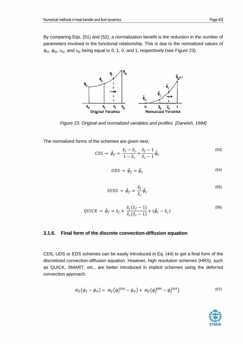
By comparing Eqs. (51) and (52), a normalization benefit is the reduction in the number of
parameters involved in the functional relationship. This is due to the normalized values of
, , , and being equal to 0, 1, 0, and 1, respectively (see Figure 23).
Figure 23. Original and normalized variables and profiles. [Darwish, 1994]
The normalized forms of the schemes are given next,
(53)
(54)
(55)
(56)
3.1.6. Final form of the discrete convection-diffusion equation
CDS, UDS or EDS schemes can be easily introduced in Eq. (44) to get a final form of the
discretized convection-diffusion equation. However, high resolution schemes (HRS), such
as QUICK, SMART, etc., are better introduced in implicit schemes using the deferred
convection approach.
(57)
Page 44 Master Thesis
Where Eq. (46) can be written as
(58)
Then Eq. (44) can finally be written as
(59)
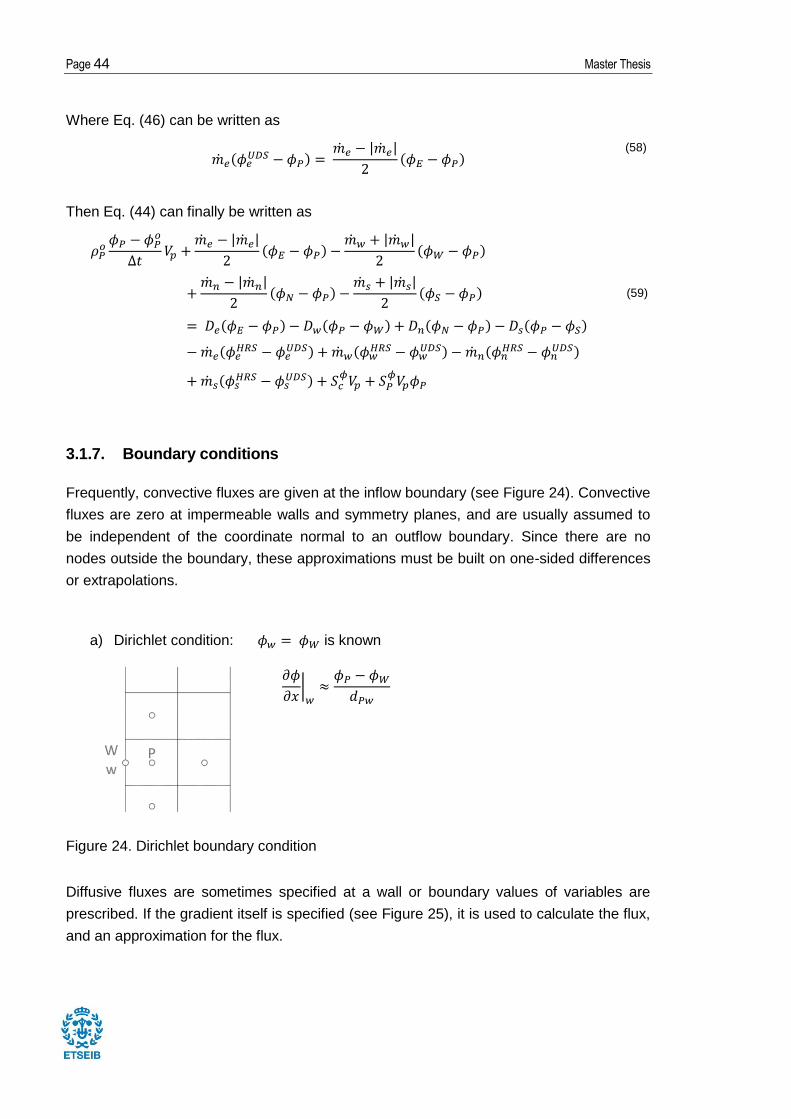
3.1.7. Boundary conditions
Frequently, convective fluxes are given at the inflow boundary (see Figure 24). Convective
fluxes are zero at impermeable walls and symmetry planes, and are usually assumed to
be independent of the coordinate normal to an outflow boundary. Since there are no
nodes outside the boundary, these approximations must be built on one-sided differences
or extrapolations.
a) Dirichlet condition: is known
Figure 24. Dirichlet boundary condition
Diffusive fluxes are sometimes specified at a wall or boundary values of variables are
prescribed. If the gradient itself is specified (see Figure 25), it is used to calculate the flux,
and an approximation for the flux.
Numerical methods in heat transfer and fluid dynamics Page 45
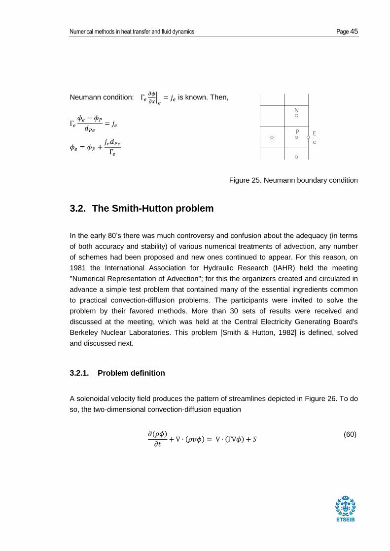
Neumann condition:
is known. Then,
Figure 25. Neumann boundary condition
3.2. The Smith-Hutton problem
In the early 80’s there was much controversy and confusion about the adequacy (in terms
of both accuracy and stability) of various numerical treatments of advection, any number
of schemes had been proposed and new ones continued to appear. For this reason, on
1981 the International Association for Hydraulic Research (IAHR) held the meeting
"Numerical Representation of Advection"; for this the organizers created and circulated in
advance a simple test problem that contained many of the essential ingredients common
to practical convection-diffusion problems. The participants were invited to solve the
problem by their favored methods. More than 30 sets of results were received and
discussed at the meeting, which was held at the Central Electricity Generating Board's
Berkeley Nuclear Laboratories. This problem [Smith & Hutton, 1982] is defined, solved
and discussed next.
3.2.1. Problem definition
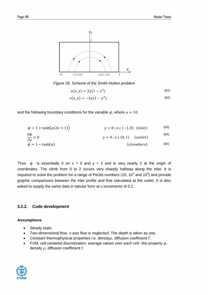
A solenoidal velocity field produces the pattern of streamlines depicted in Figure 26. To do
so, the two-dimensional convection-diffusion equation
(60)
Page 46 Master Thesis
Figure 26. Scheme of the Smith-Hutton problem
(61)
(62)
and the following boundary conditions for the variable , where .
(63)
(64)
(65)
Thus is essentially 0 on x = 0 and y = 1 and is very nearly 2 at the origin of
coordinates. The climb from 0 to 2 occurs very sharply halfway along the inlet. It is
required to solve the problem for a range of Peclet numbers (10, 103 and 106) and provide
graphic comparisons between the inlet profile and that calculated at the outlet. It is also
asked to supply the same data in tabular form at x increments of 0.1.
3.2.2. Code development
Assumptions
Steady state.
Two-dimensional flow, z-axis flow is neglected. The depth is taken as one.
Constant thermophysical properties i.e. density , diffusion coefficient .
FVM, cell-centered discretization: average values over each cell –the property ,
density , diffusion coefficient .
Numerical methods in heat transfer and fluid dynamics Page 47
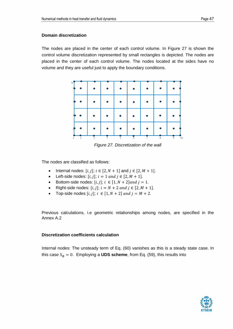
Domain discretization
The nodes are placed in the center of each control volume. In Figure 27 is shown the
control volume discretization represented by small rectangles is depicted. The nodes are
placed in the center of each control volume. The nodes located at the sides have no
volume and they are useful just to apply the boundary conditions.
Figure 27. Discretization of the wall
The nodes are classified as follows:
Internal nodes: ; and .
Left-side nodes: ;
Bottom-side nodes: ;
Right-side nodes: ;
Top-side nodes ;
Previous calculations, i.e geometric relationships among nodes, are specified in the
Annex A.2
Discretization coefficients calculation
Internal nodes: The unsteady term of Eq. (60) vanishes as this is a steady state case. In
this case . Employing a UDS scheme, from Eq. (59), this results into

Page 48 Master Thesis
(66)
Modeling Equation (66) like Eq. (25), the discretization coefficients result
(67)
(68)
(69)
(70)
(71)
(72)
As then
Moreover, using a CDS scheme:
Eq. (49) results into the final CDS equation
Numerical methods in heat transfer and fluid dynamics Page 49
(73)
Then the discretization coefficients result
(74)
(75)
(76)
(77)
(78)
(79)
For left-, right- and top-side nodes, . Then
(80)
(81)
In the case of bottom-side nodes,
. Then
(82)
(83)
And
Then
(84)
Page 50 Master Thesis
(85)
Then the discretization coefficients result
(86)
(87)
(88)
QUICK and SUDS schemes are better introduced with the previously explained ‘deferred
convection approach’11. Eq. (59) is modeled like Eq. (25). Then the discretization
coefficients result
(89)
(90)
(91)
(92)
(93)
(94)
can be computed using the normalized variables Eq. (50), Eq. (55) and
Eq.(56).
Solver
11
CDS or UDS schemes may be used in the CVs next to the sides since nodes WW, EE, SS and NN may not
exist.
Numerical methods in heat transfer and fluid dynamics Page 51
After obtaining all the discretization coefficients, the property map is obtained employing the
line-by-line methodology (see Solver in 2.2.2). This time is not the temperature, like in heat
conduction, but the property which is solved with the line-by-line method.
Then for
(95)
(96)
3.2.3. Algorithm
The algorithm proposal for the resolution of the Smith-Hutton problem is presented below.
1. Input data
Physical data: ; numerical data: , convective scheme
Geometrical data: ; boundary conditions.
2. Previous calculations12. (See Annex A2)
, ; .
3. Guess the property field
4. Calculate the discretization coefficients of all the nodes according
the convective scheme employed.
5. Calculate the property map using the line-by-line or GS solver.
6. Apply the convergence criteria: Is
a. If no, . (Refresh the guessed property map to the last
calculated map); and go to 4.
b. If yes, convergence reached. Go to 7.
7. Final calculations and print results.
12 These variables are calculated using only the input data.
Page 52 Master Thesis
3.2.4. Verification
Table 27 shows the simulation parameters used for the simulation of the Smith-Hutton
problem.
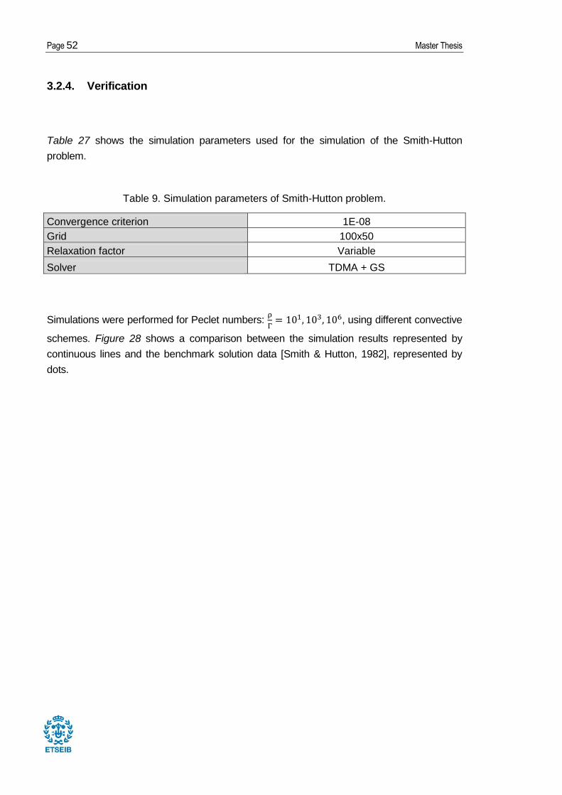
Table 9. Simulation parameters of Smith-Hutton problem.
Convergence criterion 1E-08
Grid 100x50
Relaxation factor Variable
Solver TDMA + GS
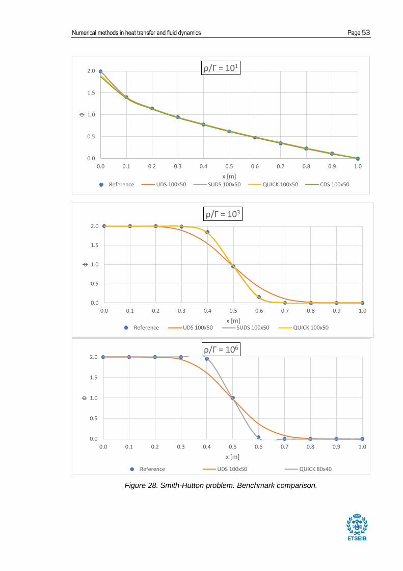
Simulations were performed for Peclet numbers:
, using different convective
schemes. Figure 28 shows a comparison between the simulation results represented by
continuous lines and the benchmark solution data [Smith & Hutton, 1982], represented by
dots.
Numerical methods in heat transfer and fluid dynamics Page 53
Figure 28. Smith-Hutton problem. Benchmark comparison.
0.0
0.5
1.0
1.5
2.0
0.0 0.1 0.2 0.3 0.4 0.5 0.6 0.7 0.8 0.9 1.0
ф
x [m]
ρ/Г = 101
Reference UDS 100x50 SUDS 100x50 QUICK 100x50 CDS 100x50
0.0
0.5
1.0
1.5
2.0
0.0 0.1 0.2 0.3 0.4 0.5 0.6 0.7 0.8 0.9 1.0
ф
x [m]
ρ/Г = 103
Reference UDS 100x50 SUDS 100x50 QUICK 100x50
0.0
0.5
1.0
1.5
2.0
0.0 0.1 0.2 0.3 0.4 0.5 0.6 0.7 0.8 0.9 1.0
ф
x [m]
ρ/Г = 106
Reference UDS 100x50 QUICK 80x40
Page 54 Master Thesis
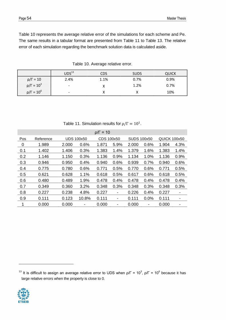
Table 10 represents the average relative error of the simulations for each scheme and Pe.
The same results in a tabular format are presented from Table 11 to Table 13. The relative
error of each simulation regarding the benchmark solution data is calculated aside.
Table 10. Average relative error.
UDS13 CDS SUDS QUICK
ρ/Г = 10 2.4% 1.1% 0.7% 0.9%
ρ/Г = 103 - X 1.2% 0.7%
ρ/Г = 106 - X X 10%
Table 11. Simulation results for .
ρ/Г = 10
Pos Reference UDS 100x50 CDS 100x50 SUDS 100x50 QUICK 100x50
0 1.989 2.000 0.6% 1.871 5.9% 2.000 0.6% 1.904 4.3%
0.1 1.402 1.406 0.3% 1.383 1.4% 1.379 1.6% 1.383 1.4%
0.2 1.146 1.150 0.3% 1.136 0.9% 1.134 1.0% 1.136 0.9%
0.3 0.946 0.950 0.4% 0.940 0.6% 0.939 0.7% 0.940 0.6%
0.4 0.775 0.780 0.6% 0.771 0.5% 0.770 0.6% 0.771 0.5%
0.5 0.621 0.628 1.1% 0.618 0.5% 0.617 0.6% 0.618 0.5%
0.6 0.480 0.489 1.9% 0.478 0.4% 0.478 0.4% 0.478 0.4%
0.7 0.349 0.360 3.2% 0.348 0.3% 0.348 0.3% 0.348 0.3%
0.8 0.227 0.238 4.8% 0.227 - 0.226 0.4% 0.227 -
0.9 0.111 0.123 10.8% 0.111 - 0.111 0.0% 0.111 -
1 0.000 0.000 - 0.000 - 0.000 - 0.000 -
13 It is difficult to assign an average relative error to UDS when ρ/Г = 10
3, ρ/Г = 10
6 because it has
large relative errors when the property is close to 0.
Numerical methods in heat transfer and fluid dynamics Page 55
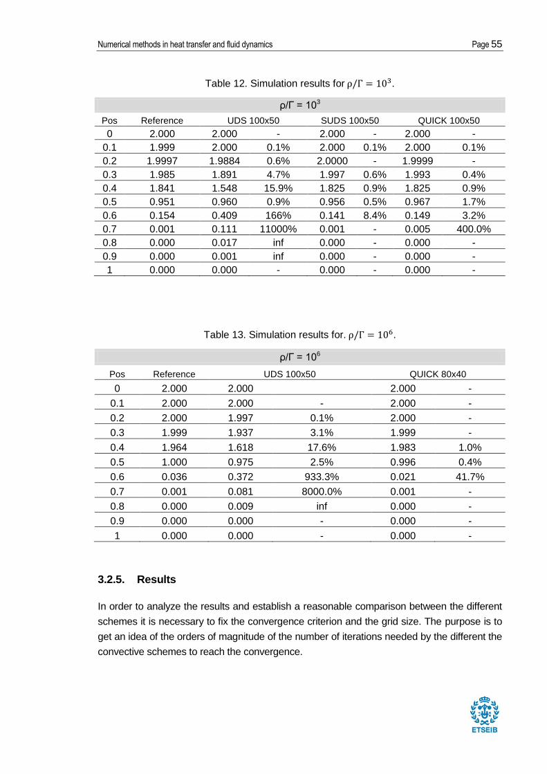
Table 12. Simulation results for .
ρ/Г = 103
Pos Reference UDS 100x50 SUDS 100x50 QUICK 100x50
0 2.000 2.000 - 2.000 - 2.000 -
0.1 1.999 2.000 0.1% 2.000 0.1% 2.000 0.1%
0.2 1.9997 1.9884 0.6% 2.0000 - 1.9999 -
0.3 1.985 1.891 4.7% 1.997 0.6% 1.993 0.4%
0.4 1.841 1.548 15.9% 1.825 0.9% 1.825 0.9%
0.5 0.951 0.960 0.9% 0.956 0.5% 0.967 1.7%
0.6 0.154 0.409 166% 0.141 8.4% 0.149 3.2%
0.7 0.001 0.111 11000% 0.001 - 0.005 400.0%
0.8 0.000 0.017 inf 0.000 - 0.000 -
0.9 0.000 0.001 inf 0.000 - 0.000 -
1 0.000 0.000 - 0.000 - 0.000 -
Table 13. Simulation results for. .
ρ/Г = 106
Pos Reference UDS 100x50 QUICK 80x40
0 2.000 2.000
2.000 -
0.1 2.000 2.000 - 2.000 -
0.2 2.000 1.997 0.1% 2.000 -
0.3 1.999 1.937 3.1% 1.999 -
0.4 1.964 1.618 17.6% 1.983 1.0%
0.5 1.000 0.975 2.5% 0.996 0.4%
0.6 0.036 0.372 933.3% 0.021 41.7%
0.7 0.001 0.081 8000.0% 0.001 -
0.8 0.000 0.009 inf 0.000 -
0.9 0.000 0.000 - 0.000 -
1 0.000 0.000 - 0.000 -
3.2.5. Results
In order to analyze the results and establish a reasonable comparison between the different
schemes it is necessary to fix the convergence criterion and the grid size. The purpose is to
get an idea of the orders of magnitude of the number of iterations needed by the different the
convective schemes to reach the convergence.
Page 56 Master Thesis
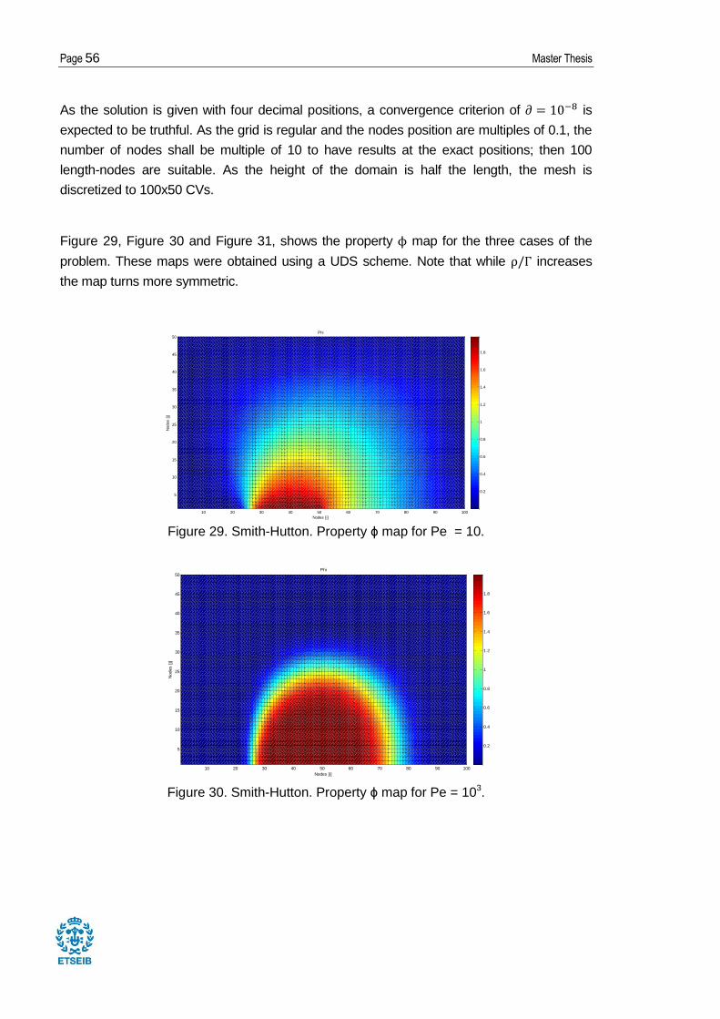
As the solution is given with four decimal positions, a convergence criterion of is
expected to be truthful. As the grid is regular and the nodes position are multiples of 0.1, the
number of nodes shall be multiple of 10 to have results at the exact positions; then 100
length-nodes are suitable. As the height of the domain is half the length, the mesh is
discretized to 100x50 CVs.
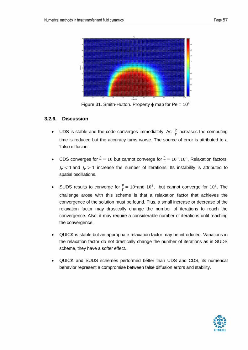
Figure 29, Figure 30 and Figure 31, shows the property map for the three cases of the
problem. These maps were obtained using a UDS scheme. Note that while increases
the map turns more symmetric.
Figure 29. Smith-Hutton. Property ϕ map for Pe = 10.
Figure 30. Smith-Hutton. Property ϕ map for Pe = 103.
10 20 30 40 50 60 70 80 90 100
5
10
15
20
25
30
35
40
45
50
Nodes [
j]
Nodes [i]
Phi
0.2
0.4
0.6
0.8
1
1.2
1.4
1.6
1.8
10 20 30 40 50 60 70 80 90 100
5
10
15
20
25
30
35
40
45
50
Nodes [
j]
Nodes [i]
Phi
0.2
0.4
0.6
0.8
1
1.2
1.4
1.6
1.8
Numerical methods in heat transfer and fluid dynamics Page 57
Figure 31. Smith-Hutton. Property ϕ map for Pe = 106.
3.2.6. Discussion
UDS is stable and the code converges immediately. As
increases the computing
time is reduced but the accuracy turns worse. The source of error is attributed to a
‘false diffusion’.
CDS converges for
but cannot converge for
. Relaxation factors,
and increase the number of iterations. Its instability is attributed to
spatial oscillations.
SUDS results to converge for
and , but cannot converge for . The
challenge arose with this scheme is that a relaxation factor that achieves the
convergence of the solution must be found. Plus, a small increase or decrease of the
relaxation factor may drastically change the number of iterations to reach the
convergence. Also, it may require a considerable number of iterations until reaching
the convergence.
QUICK is stable but an appropriate relaxation factor may be introduced. Variations in
the relaxation factor do not drastically change the number of iterations as in SUDS
scheme, they have a softer effect.
QUICK and SUDS schemes performed better than UDS and CDS, its numerical
behavior represent a compromise between false diffusion errors and stability.
10 20 30 40 50 60 70 80 90 100
5
10
15
20
25
30
35
40
45
50
Nodes [
j]
Nodes [i]
Phi
0.2
0.4
0.6
0.8
1
1.2
1.4
1.6
1.8
Page 58 Master Thesis
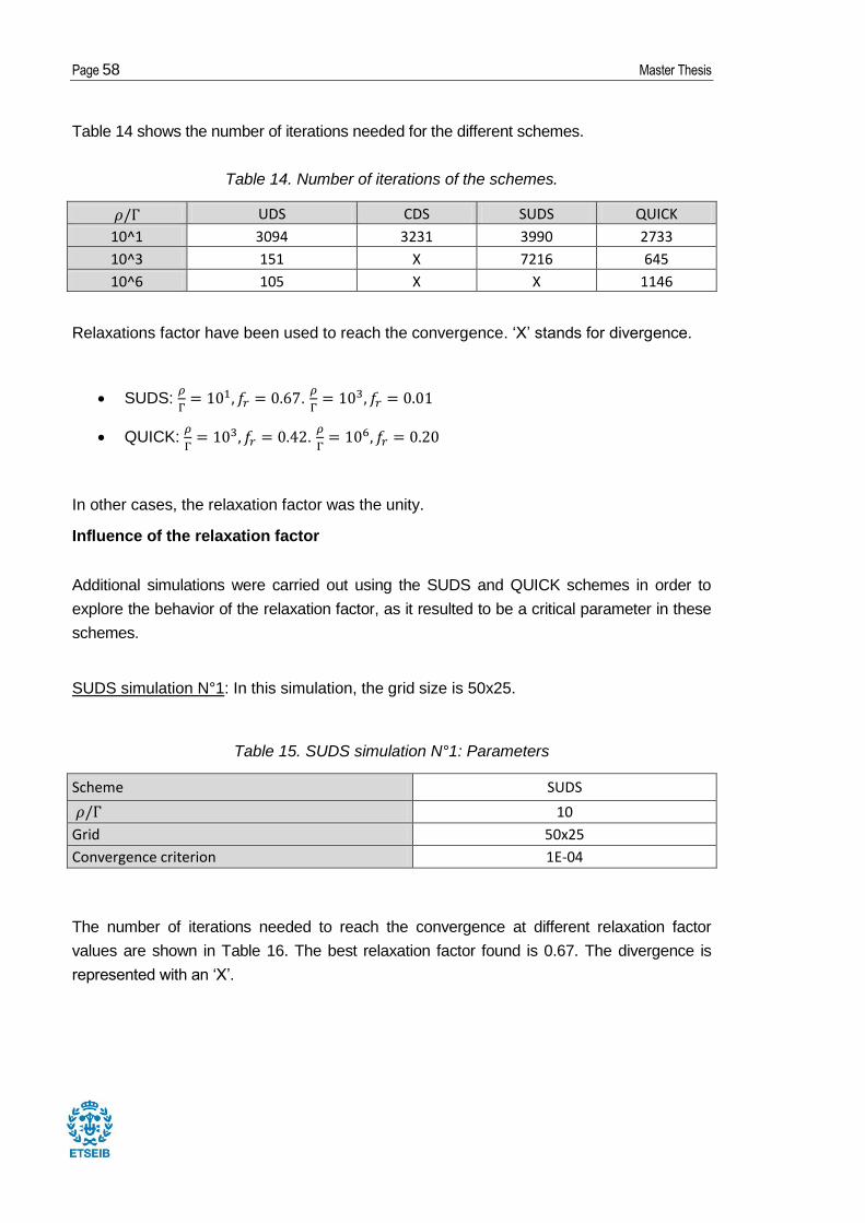
Table 14 shows the number of iterations needed for the different schemes.
Table 14. Number of iterations of the schemes.
UDS CDS SUDS QUICK
10^1 3094 3231 3990 2733
10^3 151 X 7216 645
10^6 105 X X 1146
Relaxations factor have been used to reach the convergence. ‘X’ stands for divergence.
SUDS:
.
QUICK:
.
In other cases, the relaxation factor was the unity.
Influence of the relaxation factor
Additional simulations were carried out using the SUDS and QUICK schemes in order to
explore the behavior of the relaxation factor, as it resulted to be a critical parameter in these
schemes.
SUDS simulation N°1: In this simulation, the grid size is 50x25.
Table 15. SUDS simulation N°1: Parameters
Scheme SUDS
10
Grid 50x25
Convergence criterion 1E-04
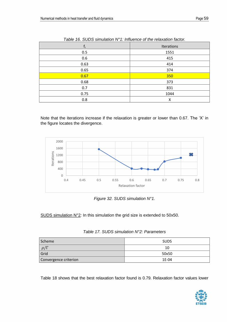
The number of iterations needed to reach the convergence at different relaxation factor
values are shown in Table 16. The best relaxation factor found is 0.67. The divergence is
represented with an ‘X’.
Numerical methods in heat transfer and fluid dynamics Page 59
Table 16. SUDS simulation N°1: Influence of the relaxation factor.
fr Iterations
0.5 1551
0.6 415
0.63 414
0.65 374
0.67 350
0.68 373
0.7 831
0.75 1044
0.8 X
Note that the iterations increase if the relaxation is greater or lower than 0.67. The ‘X’ in
the figure locates the divergence.
Figure 32. SUDS simulation N°1.
SUDS simulation N°2: In this simulation the grid size is extended to 50x50.
Table 17. SUDS simulation N°2: Parameters
Scheme SUDS
10
Grid 50x50
Convergence criterion 1E-04
Table 18 shows that the best relaxation factor found is 0.79. Relaxation factor values lower
0
400
800
1200
1600
2000
0.4 0.45 0.5 0.55 0.6 0.65 0.7 0.75 0.8
Iter
atio
ns
Relaxation factor
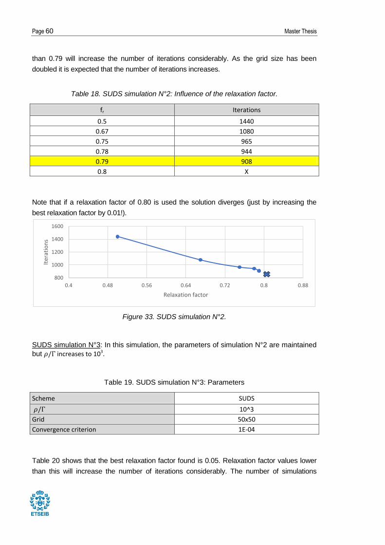
Page 60 Master Thesis
than 0.79 will increase the number of iterations considerably. As the grid size has been
doubled it is expected that the number of iterations increases.
Table 18. SUDS simulation N°2: Influence of the relaxation factor.
fr Iterations
0.5 1440
0.67 1080
0.75 965
0.78 944
0.79 908
0.8 X
Note that if a relaxation factor of 0.80 is used the solution diverges (just by increasing the
best relaxation factor by 0.01!).
Figure 33. SUDS simulation N°2.
SUDS simulation N°3: In this simulation, the parameters of simulation N°2 are maintained
but increases to 103.
Table 19. SUDS simulation N°3: Parameters
Scheme SUDS
10^3
Grid 50x50
Convergence criterion 1E-04
Table 20 shows that the best relaxation factor found is 0.05. Relaxation factor values lower
than this will increase the number of iterations considerably. The number of simulations
800
1000
1200
1400
1600
0.4 0.48 0.56 0.64 0.72 0.8 0.88
Iter
atio
ns
Relaxation factor
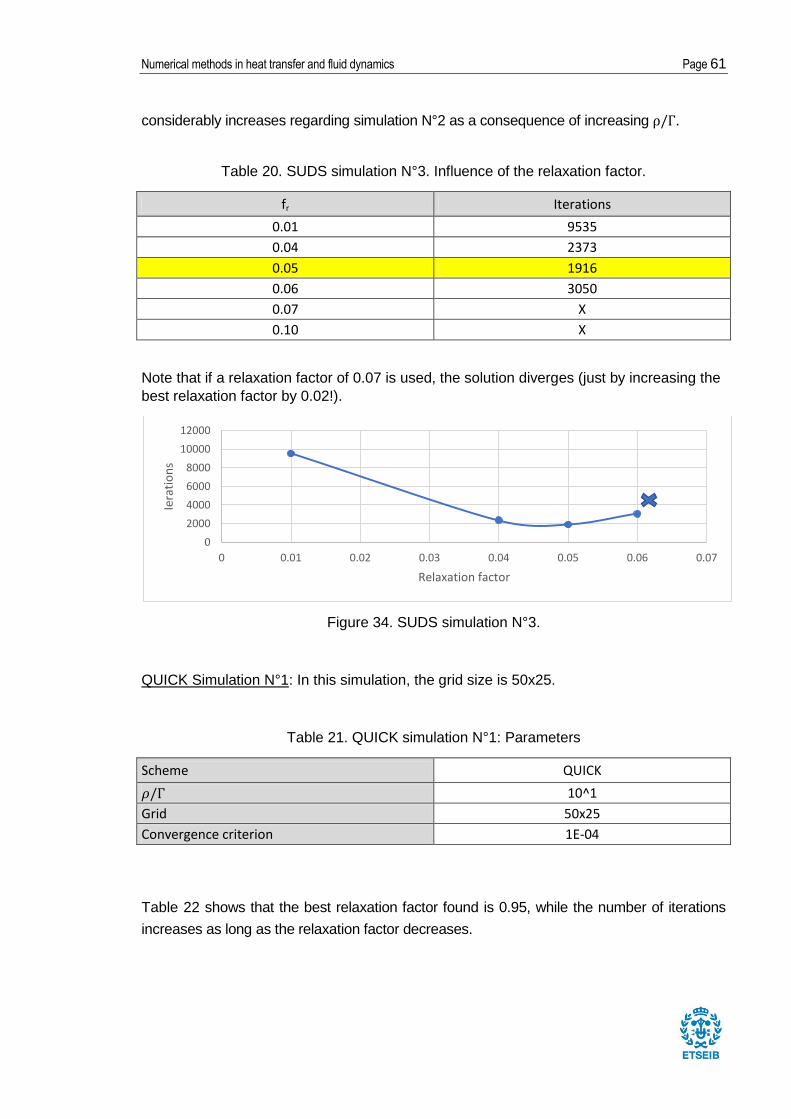
Numerical methods in heat transfer and fluid dynamics Page 61
considerably increases regarding simulation N°2 as a consequence of increasing .
Table 20. SUDS simulation N°3. Influence of the relaxation factor.
fr Iterations
0.01 9535
0.04 2373
0.05 1916
0.06 3050
0.07 X
0.10 X
Note that if a relaxation factor of 0.07 is used, the solution diverges (just by increasing the
best relaxation factor by 0.02!).
Figure 34. SUDS simulation N°3.
QUICK Simulation N°1: In this simulation, the grid size is 50x25.
Table 21. QUICK simulation N°1: Parameters
Scheme QUICK
10^1
Grid 50x25
Convergence criterion 1E-04
Table 22 shows that the best relaxation factor found is 0.95, while the number of iterations
increases as long as the relaxation factor decreases.
0
2000
4000
6000
8000
10000
12000
0 0.01 0.02 0.03 0.04 0.05 0.06 0.07
Iera
tio
ns
Relaxation factor
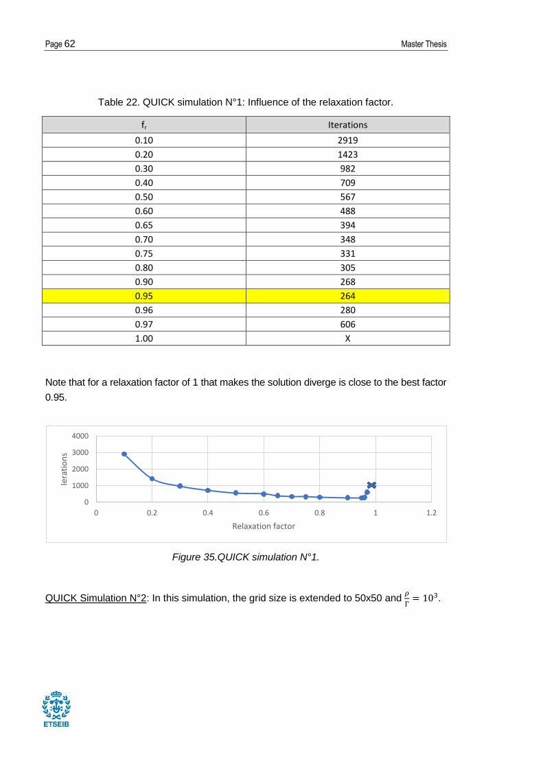
Page 62 Master Thesis
Table 22. QUICK simulation N°1: Influence of the relaxation factor.
fr Iterations
0.10 2919
0.20 1423
0.30 982
0.40 709
0.50 567
0.60 488
0.65 394
0.70 348
0.75 331
0.80 305
0.90 268
0.95 264
0.96 280
0.97 606
1.00 X
Note that for a relaxation factor of 1 that makes the solution diverge is close to the best factor
0.95.
Figure 35.QUICK simulation N°1.
QUICK Simulation N°2: In this simulation, the grid size is extended to 50x50 and
.
0
1000
2000
3000
4000
0 0.2 0.4 0.6 0.8 1 1.2
Iera
tio
ns
Relaxation factor
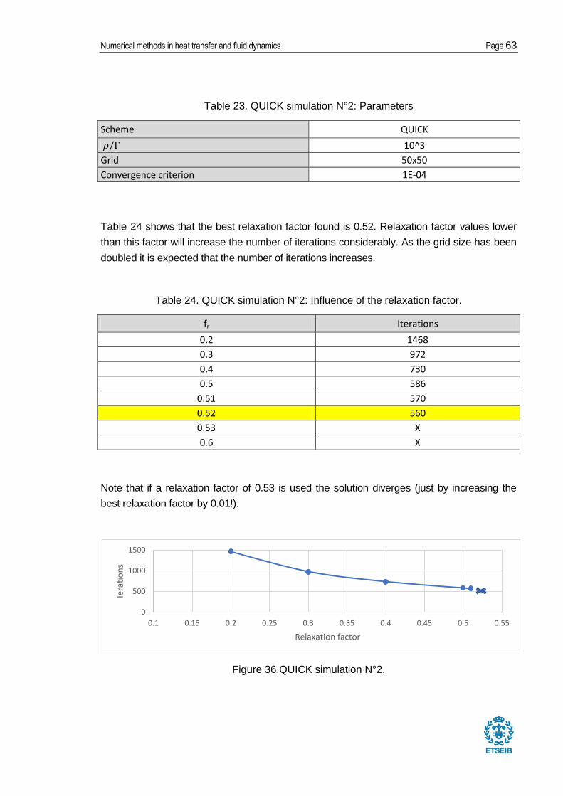
Numerical methods in heat transfer and fluid dynamics Page 63
Table 23. QUICK simulation N°2: Parameters
Scheme QUICK
10^3
Grid 50x50
Convergence criterion 1E-04
Table 24 shows that the best relaxation factor found is 0.52. Relaxation factor values lower
than this factor will increase the number of iterations considerably. As the grid size has been
doubled it is expected that the number of iterations increases.
Table 24. QUICK simulation N°2: Influence of the relaxation factor.
fr Iterations
0.2 1468
0.3 972
0.4 730
0.5 586
0.51 570
0.52 560
0.53 X
0.6 X
Note that if a relaxation factor of 0.53 is used the solution diverges (just by increasing the
best relaxation factor by 0.01!).
Figure 36.QUICK simulation N°2.
0
500
1000
1500
0.1 0.15 0.2 0.25 0.3 0.35 0.4 0.45 0.5 0.55
Iera
tio
ns
Relaxation factor
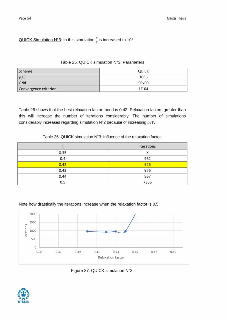
Page 64 Master Thesis
QUICK Simulation N°3: In this simulation
is increased to .
Table 25. QUICK simulation N°3: Parameters
Scheme QUICK
10^6
Grid 50x50
Convergence criterion 1E-04
Table 26 shows that the best relaxation factor found is 0.42. Relaxation factors greater than
this will increase the number of iterations considerably. The number of simulations
considerably increases regarding simulation N°2 because of increasing .
Table 26. QUICK simulation N°3: Influence of the relaxation factor.
fr Iterations
0.35 X
0.4 962
0.42 926
0.43 956
0.44 967
0.5 7356
Note how drastically the iterations increase when the relaxation factor is 0.5
Figure 37. QUICK simulation N°3.
0
500
1000
1500
2000
0.35 0.37 0.39 0.41 0.43 0.45 0.47 0.49
Iera
tio
ns
Relaxation factor
Numerical methods in heat transfer and fluid dynamics Page 65
4. Incompressible flow method using the Navier-
Stokes equations
This chapter shows how the classical fractional step projection method [Chorin, 1968;
Temam, 1969; Yanenko, 1971] is applied to incompressible flows of Newtonian fluids to
solve the velocity-pressure coupling in the NSE14. The fractional step method (FSM) provides
an approach that does not use pressure in a predictor step to estimate the projected velocity,
an approximate solution of the momentum equation. Consequently, it is required to couple a
pressure equation which determines the minimum perturbation that will make the predictor
velocity incompressible. It is also important to recall that the role of the pressure in an
incompressible flow is to enforce continuity; in some sense, it is more a mathematical
variable than a physical one. [Ferziger, 2002].
There are two main goals of this chapter; the first is to depict the FSM employing staggered
meshes for its solution, and the second is to assess the performance the numerical schemes
presented in Section 3.1.4 in the solution of a model problem, the driven cavity flow. [Ghia,
1982].
4.1. Introduction to the Fractional Step Method
The simulation of incompressible flows of Newtonian fluids is considered. Under these
assumptions, the dimensionless governing NS equations in primitive variables are:
(97)
(98)
where Re is the dimensionless Reynolds number defined as
(99)
14 High accurate numerical solutions have evidenced that these equations form an excellent
mathematical model for turbulent flow. However, more than one and a half century later the
understanding of them remains minimal. For instance, the existence and uniqueness of general
solutions remains an open question. [CTTC, 2017]
Page 66 Master Thesis
And and are the density and the dynamic viscosity of the working fluid; and are the
characteristic length and velocity, respectively.
4.1.1. Application of the Helmholtz-Hodge decomposition theorem
In this section, the Helmholtz-Hodge decomposition theorem is applied to the incompressible
NSE. The results here obtained will help us to better elucidate the role of the pressure field.
According to the Helmholtz-Hodge theorem, a given vector field ω, defined in a bounded
domain with smooth boundary , is uniquely decomposed in a pure gradient field and a
divergence-free vector parallel to .
(100)
where,
(101)
The theorem also applies for periodic inflow/outflow conditions.
Let be a projector operator. It projects any vector field onto a divergence-free space15
(102)
Now, taking the NS equations and applying the projector operator
(103)
Since the velocity field is incompressible the transient term remains unchanged (see Eq. I)
when projected
15 Note that any incompressible field remains unchanged by the action of the projector operator ,
(I)
moreover, the projector operator , has the following property
(II)
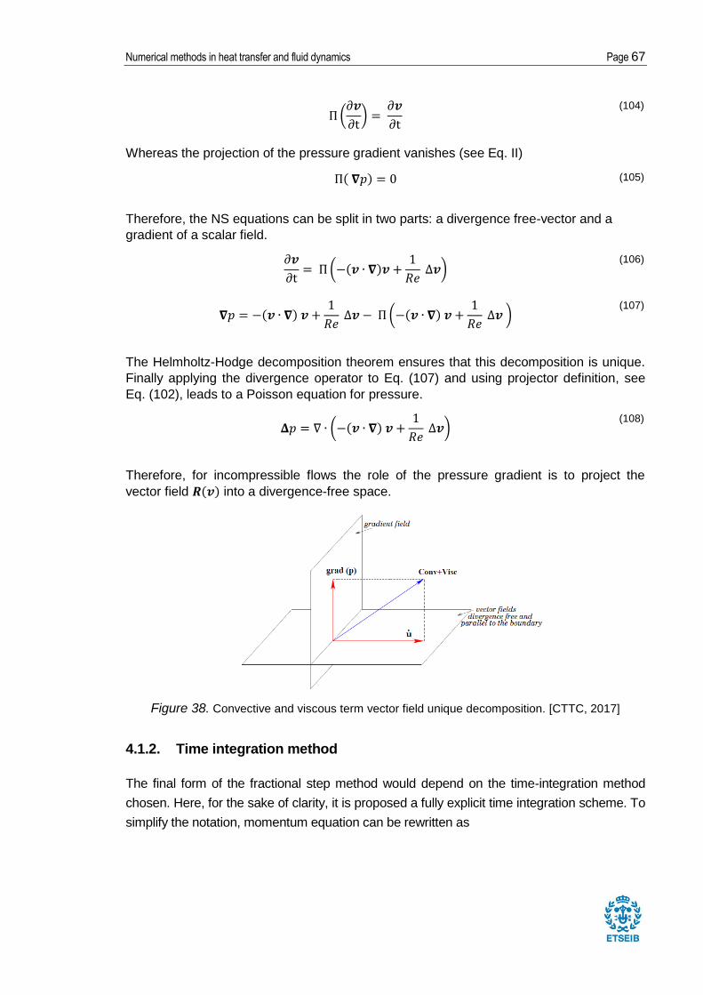
Numerical methods in heat transfer and fluid dynamics Page 67
(104)
Whereas the projection of the pressure gradient vanishes (see Eq. II)
(105)
Therefore, the NS equations can be split in two parts: a divergence free-vector and a
gradient of a scalar field.
(106)
(107)
The Helmholtz-Hodge decomposition theorem ensures that this decomposition is unique.
Finally applying the divergence operator to Eq. (107) and using projector definition, see
Eq. (102), leads to a Poisson equation for pressure.
(108)
Therefore, for incompressible flows the role of the pressure gradient is to project the
vector field into a divergence-free space.
Figure 38. Convective and viscous term vector field unique decomposition. [CTTC, 2017]
4.1.2. Time integration method
The final form of the fractional step method would depend on the time-integration method
chosen. Here, for the sake of clarity, it is proposed a fully explicit time integration scheme. To
simplify the notation, momentum equation can be rewritten as
Page 68 Master Thesis
(109)
where stands for the convective and diffusive terms
(110)
For the temporal discretization, a central difference scheme is used for the time derivative
term,
(111)
a fully explicit second-order Adams-Bashforth scheme for
(112)
and a first order backward Euler scheme for the pressure-gradient term. Incompressibility
constraint is treated implicitly. Thus, we obtain the semi-discretized NSE.
(113)
(114)
Then, the pressure gradient forces (projects) the predictor velocity field to be
incompressible . This projection is derived from the well-known Helmholtz-
Hodge vector decomposition theorem, whereby the predictor velocity , can be uniquely
decomposed into a divergence-free vector, , and the gradient of a scalar field, . This
decomposition is written as
(115)
where the predictor velocity is given by
(116)
and the pseudo-pressure is Taking the divergence of Eq. (115) yields a Poisson
equation for .
Numerical methods in heat transfer and fluid dynamics Page 69
(117)
Once the solution is obtained, results from the correction
(118)
Therefore, the algorithm for the integration of each time step is
1. Evaluate .
2. Evaluate from Eq. (116).
3. Evaluate and solve the discrete Poisson equation, Eq. (117).
4. Obtain the new velocity field with Eq.(118).
4.1.3. Determination of
Due to stability reasons, explicit temporal schemes introduce severe restrictions on the time
step, while implicit discretization would improve the overall stability. Here, we have only
considered explicit method in the view of formulation simplicity. Therefore, in our case, the
time-step, , must be bounded by the CFL condition [Courant, 1928] given by
(119)
(120)
where the bounding values are must be smaller than unity. In our case, we will
follow the recommendations given by Simons (2000) using values and
, respectively.16
4.1.4. The Poisson equation
Since the formulation is fully explicit, the only system to be solved is the pressure Poisson
Eq. (115). An efficient solution of the Poisson equation is critical since it may consume a
16 Note that, since the mesh would remain constant during all the simulation, only the CFL-condition for
the convective term, see Eq. (119), has to be recomputed each time-step.
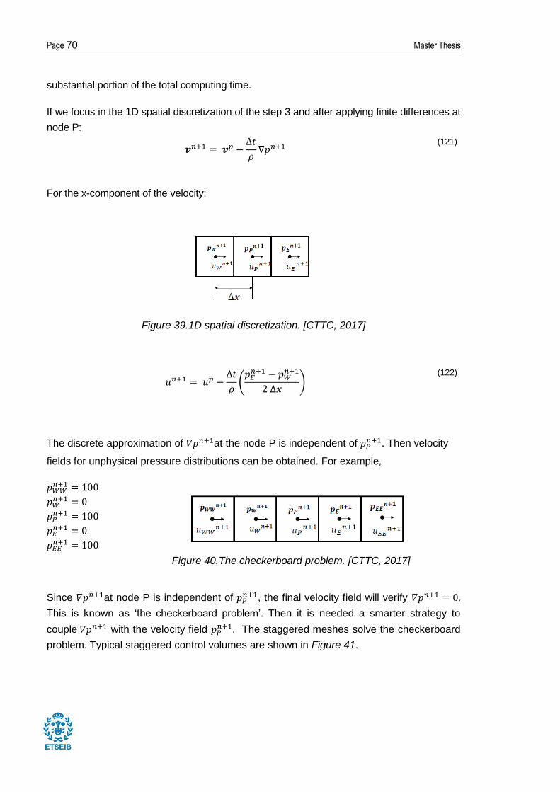
Page 70 Master Thesis
substantial portion of the total computing time.
If we focus in the 1D spatial discretization of the step 3 and after applying finite differences at
node P:
(121)
For the x-component of the velocity:
Figure 39.1D spatial discretization. [CTTC, 2017]
(122)
The discrete approximation of at the node P is independent of . Then velocity
fields for unphysical pressure distributions can be obtained. For example,
Since at node P is independent of , the final velocity field will verify
This is known as ‘the checkerboard problem’. Then it is needed a smarter strategy to
couple with the velocity field . The staggered meshes solve the checkerboard
problem. Typical staggered control volumes are shown in Figure 41.
Figure 40.The checkerboard problem. [CTTC, 2017]
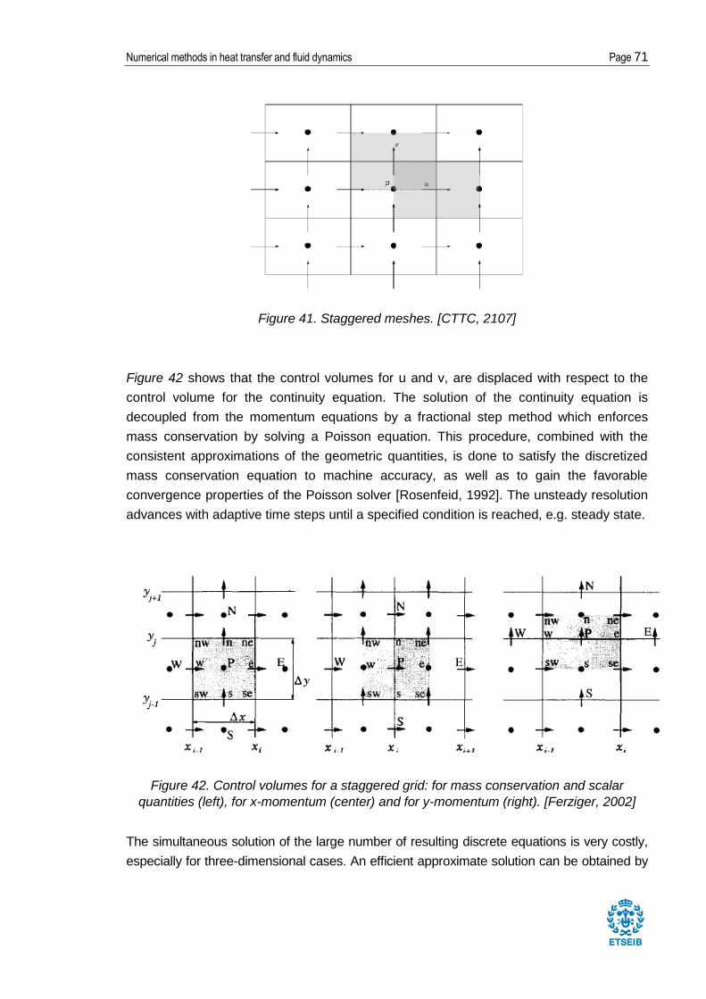
Numerical methods in heat transfer and fluid dynamics Page 71
Figure 41. Staggered meshes. [CTTC, 2107]
Figure 42 shows that the control volumes for u and v, are displaced with respect to the
control volume for the continuity equation. The solution of the continuity equation is
decoupled from the momentum equations by a fractional step method which enforces
mass conservation by solving a Poisson equation. This procedure, combined with the
consistent approximations of the geometric quantities, is done to satisfy the discretized
mass conservation equation to machine accuracy, as well as to gain the favorable
convergence properties of the Poisson solver [Rosenfeid, 1992]. The unsteady resolution
advances with adaptive time steps until a specified condition is reached, e.g. steady state.
Figure 42. Control volumes for a staggered grid: for mass conservation and scalar
quantities (left), for x-momentum (center) and for y-momentum (right). [Ferziger, 2002]
The simultaneous solution of the large number of resulting discrete equations is very costly,
especially for three-dimensional cases. An efficient approximate solution can be obtained by
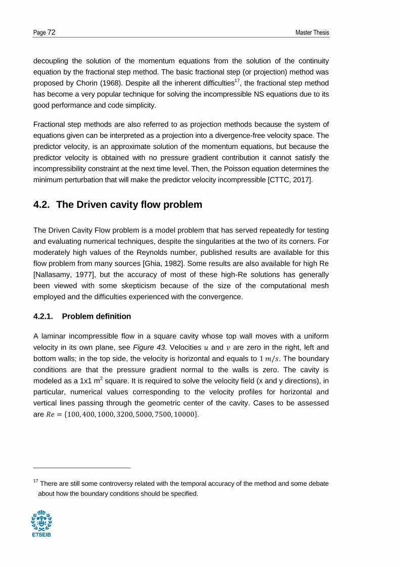
Page 72 Master Thesis
decoupling the solution of the momentum equations from the solution of the continuity
equation by the fractional step method. The basic fractional step (or projection) method was
proposed by Chorin (1968). Despite all the inherent difficulties17, the fractional step method
has become a very popular technique for solving the incompressible NS equations due to its
good performance and code simplicity.
Fractional step methods are also referred to as projection methods because the system of
equations given can be interpreted as a projection into a divergence-free velocity space. The
predictor velocity, is an approximate solution of the momentum equations, but because the
predictor velocity is obtained with no pressure gradient contribution it cannot satisfy the
incompressibility constraint at the next time level. Then, the Poisson equation determines the
minimum perturbation that will make the predictor velocity incompressible [CTTC, 2017].
4.2. The Driven cavity flow problem
The Driven Cavity Flow problem is a model problem that has served repeatedly for testing
and evaluating numerical techniques, despite the singularities at the two of its corners. For
moderately high values of the Reynolds number, published results are available for this
flow problem from many sources [Ghia, 1982]. Some results are also available for high Re
[Nallasamy, 1977], but the accuracy of most of these high-Re solutions has generally
been viewed with some skepticism because of the size of the computational mesh
employed and the difficulties experienced with the convergence.
4.2.1. Problem definition
A laminar incompressible flow in a square cavity whose top wall moves with a uniform
velocity in its own plane, see Figure 43. Velocities and are zero in the right, left and
bottom walls; in the top side, the velocity is horizontal and equals to . The boundary
conditions are that the pressure gradient normal to the walls is zero. The cavity is
modeled as a 1x1 m2 square. It is required to solve the velocity field (x and y directions), in
particular, numerical values corresponding to the velocity profiles for horizontal and
vertical lines passing through the geometric center of the cavity. Cases to be assessed
are .
17 There are still some controversy related with the temporal accuracy of the method and some debate
about how the boundary conditions should be specified.
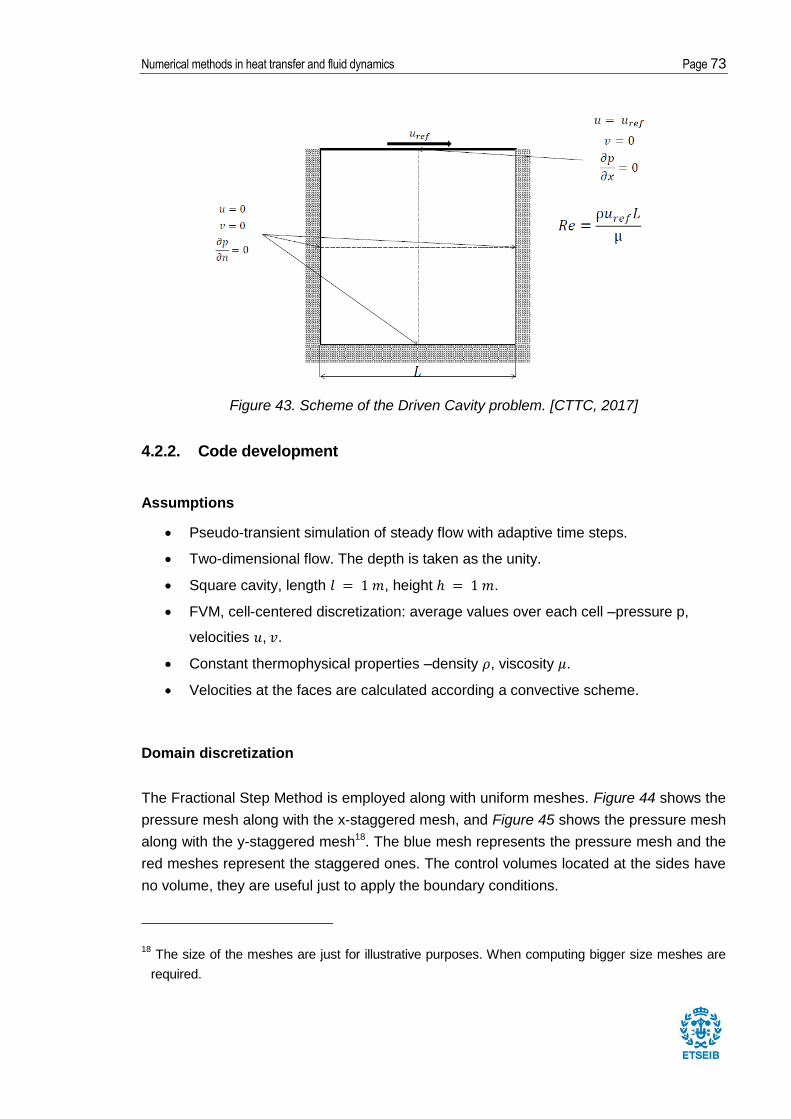
Numerical methods in heat transfer and fluid dynamics Page 73
Figure 43. Scheme of the Driven Cavity problem. [CTTC, 2017]
4.2.2. Code development
Assumptions
Pseudo-transient simulation of steady flow with adaptive time steps.
Two-dimensional flow. The depth is taken as the unity.
Square cavity, length , height .
FVM, cell-centered discretization: average values over each cell –pressure p,
velocities , .
Constant thermophysical properties –density , viscosity .
Velocities at the faces are calculated according a convective scheme.
Domain discretization
The Fractional Step Method is employed along with uniform meshes. Figure 44 shows the
pressure mesh along with the x-staggered mesh, and Figure 45 shows the pressure mesh
along with the y-staggered mesh18. The blue mesh represents the pressure mesh and the
red meshes represent the staggered ones. The control volumes located at the sides have
no volume, they are useful just to apply the boundary conditions.
18 The size of the meshes are just for illustrative purposes. When computing bigger size meshes are
required.

Page 74 Master Thesis
In this example, if we count all the control volumes, the dimensions of the pressure mesh
are 10x10, the dimensions of the x-staggered mesh are 9x10, and the dimensions of the
y-staggered mesh are 10x9, as the figures show. Alternatively, if only the non-zero control
volumes are considered, the pressure mesh in this example has dimensions 8x8, which is
the nomenclature used in this project to refer the mesh size.
Figure 44. Staggered-x mesh and pressure mesh.
Figure 45. Staggered-y mesh and pressure mesh.
Numerical methods in heat transfer and fluid dynamics Page 75
In the present text, N and M stand for the non-zero control volumes. In this way the
dimensions of the pressure mesh are (N+2) x (M+2) considering all the control volumes,
the dimensions of the x-staggered mesh is (N+1) x (M+2), and the dimensions of the y-
staggered mesh is (N+2) x (M+1).
Previous calculations
The construction of the meshes and their geometrical relations is analogous to the ones of
the ‘Smith-Hutton problem’. The node positions, relative distances, and surfaces are listed
below for the three meshes:
Pressure mesh
x-staggered mesh
y-staggered mesh
Equations discretization
At each time step the following equations give a unique and .
1.
2.
3.
4. New )
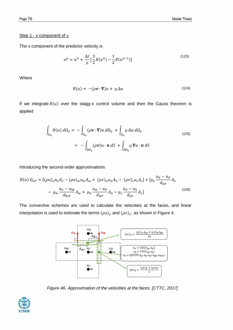
Page 76 Master Thesis
Step 1 - x component of
The x component of the predictor velocity is
(123)
Where
(124)
If we integrate over the stagg-x control volume and then the Gauss theorem is
applied
(125)
Introducing the second-order approximations
(126)
The convective schemes are used to calculate the velocities at the faces, and linear
interpolation is used to estimate the terms and , as shown in Figure 4.
Figure 46. Approximation of the velocities at the faces. [CTTC, 2017]

Numerical methods in heat transfer and fluid dynamics Page 77
Step 1 FSM - y component of
Following the same procedure, the y component of the predictor velocity is
(127)
Where
(128)
If we integrate over the stagg-y control volume and then the Gauss theorem is
applied:
(129)
Introducing the second-order approximations
(130)
Step 2 - Pressure mesh
(131)
If we integrate over the control volume and then the Gauss theorem is applied:
(132)
(133)
Page 78 Master Thesis
Introducing the second-order approximations
(134)
Adopting the FVM method form:
(135)
The discretization coefficients result
(136)
(137)
(138)
(139)
(140)
(141)
Any of the linear can be used here (GS or line-by-line).
Step 2 - Boundary conditions
Prescribed velocity
From
, if is known, we can set , thus,
.

Numerical methods in heat transfer and fluid dynamics Page 79
Figure 47. Boundary condition: prescribed velocity. [CTTC, 2017]
Step 3 - Staggered-x mesh
Figure 48. Geometric relation of the pressure mesh and the x-staggered mesh. [CTTC,
2017]
Note that for the velocity of the x-staggered mesh, and
are the correspondent pressures for and
respectively. Likewise,
corresponds to .
Step 3 - Staggered-y mesh
Figure 49. Geometric relation of the pressure mesh and the y-staggered mesh. [CTTC,
2017]
Page 80 Master Thesis
Note that for a velocity at the x-staggered mesh, and are
the correspondent pressures for and
respectively. Likewise,
corresponds to .
Step 4 - Choice of the time step.
The CFL (Courant-Friedrich-Levy) condition
(142)
(143)
(144)
4.2.3. Algorithm
The algorithm proposal for the resolution of the Driven cavity flow problem is presented
below.
[1] Input data
Physical data:
Numerical data: , , convective scheme.
Geometrical data:
Boundary conditions. at boundaries, except at the upper
boundary.
[2] Previous calculations
Creation of the regular mesh for the pressure.
Creation of the staggered-x mesh for x-velocity.
Creation of the staggered-y mesh for y-velocity.
Velocity fields creation:
Calculation of
[3] Calculation of the predictor velocities:
3.1
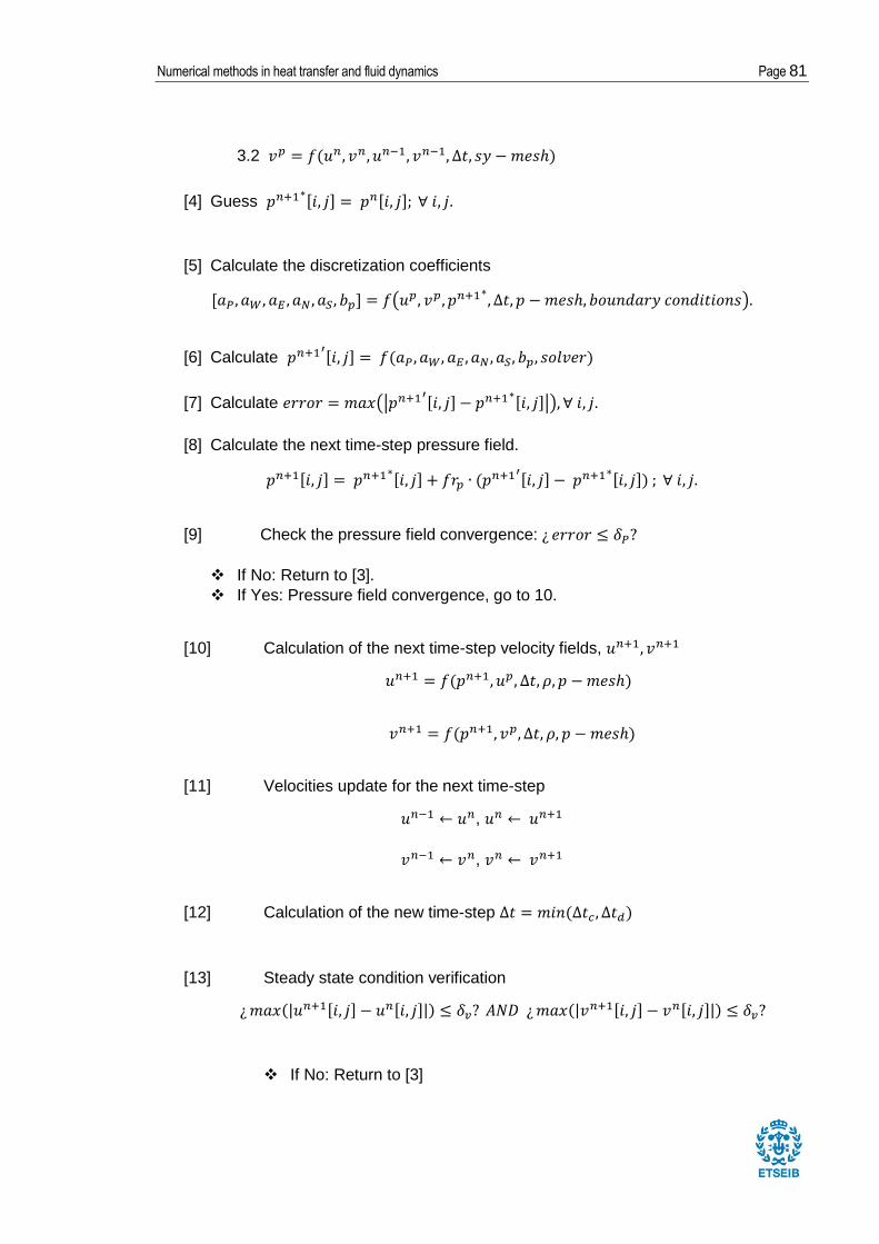
Numerical methods in heat transfer and fluid dynamics Page 81
3.2
[4] Guess
[5] Calculate the discretization coefficients
[6] Calculate
[7] Calculate
[8] Calculate the next time-step pressure field.
[9] Check the pressure field convergence:
If No: Return to [3].
If Yes: Pressure field convergence, go to 10.
[10] Calculation of the next time-step velocity fields,
[11] Velocities update for the next time-step
,
,
[12] Calculation of the new time-step
[13] Steady state condition verification
If No: Return to [3]
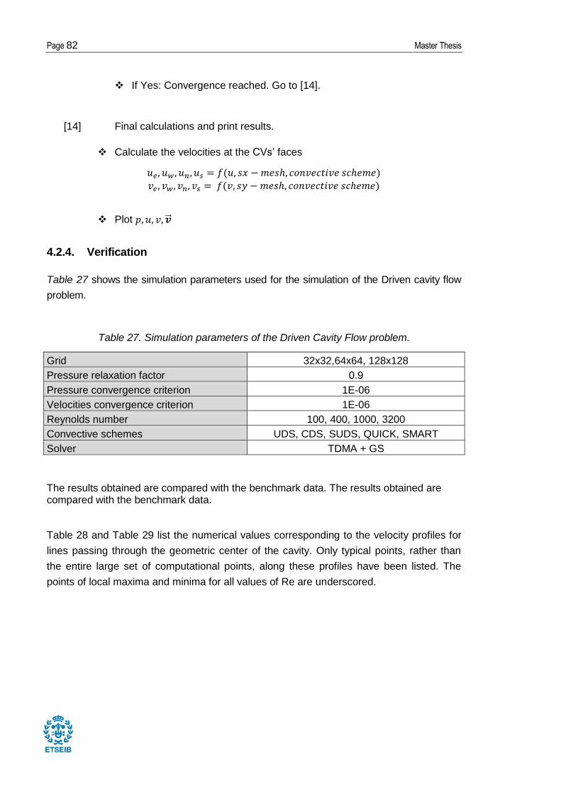
Page 82 Master Thesis
If Yes: Convergence reached. Go to [14].
[14] Final calculations and print results.
Calculate the velocities at the CVs’ faces
Plot
4.2.4. Verification
Table 27 shows the simulation parameters used for the simulation of the Driven cavity flow
problem.
Table 27. Simulation parameters of the Driven Cavity Flow problem.
Grid 32x32,64x64, 128x128
Pressure relaxation factor 0.9
Pressure convergence criterion 1E-06
Velocities convergence criterion 1E-06
Reynolds number 100, 400, 1000, 3200
Convective schemes UDS, CDS, SUDS, QUICK, SMART
Solver TDMA + GS
The results obtained are compared with the benchmark data. The results obtained are compared with the benchmark data.
Table 28 and Table 29 list the numerical values corresponding to the velocity profiles for
lines passing through the geometric center of the cavity. Only typical points, rather than
the entire large set of computational points, along these profiles have been listed. The
points of local maxima and minima for all values of Re are underscored.
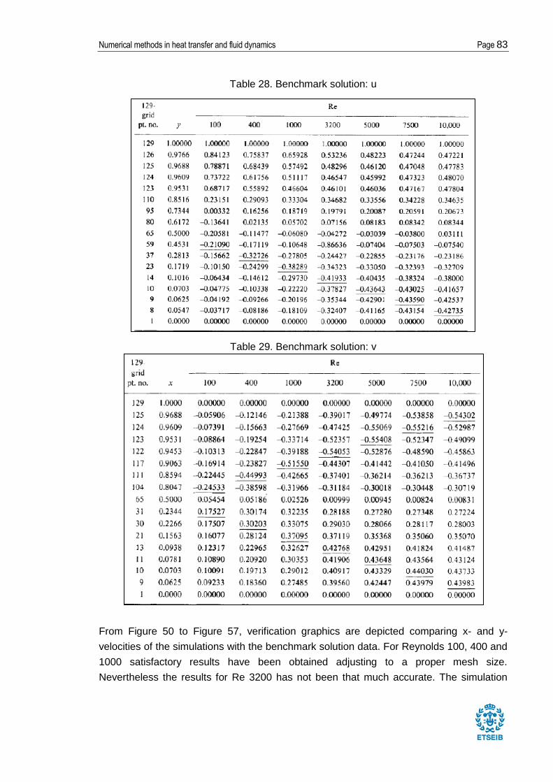
Numerical methods in heat transfer and fluid dynamics Page 83
Table 28. Benchmark solution: u
Table 29. Benchmark solution: v
From Figure 50 to Figure 57, verification graphics are depicted comparing x- and y-
velocities of the simulations with the benchmark solution data. For Reynolds 100, 400 and
1000 satisfactory results have been obtained adjusting to a proper mesh size.
Nevertheless the results for Re 3200 has not been that much accurate. The simulation
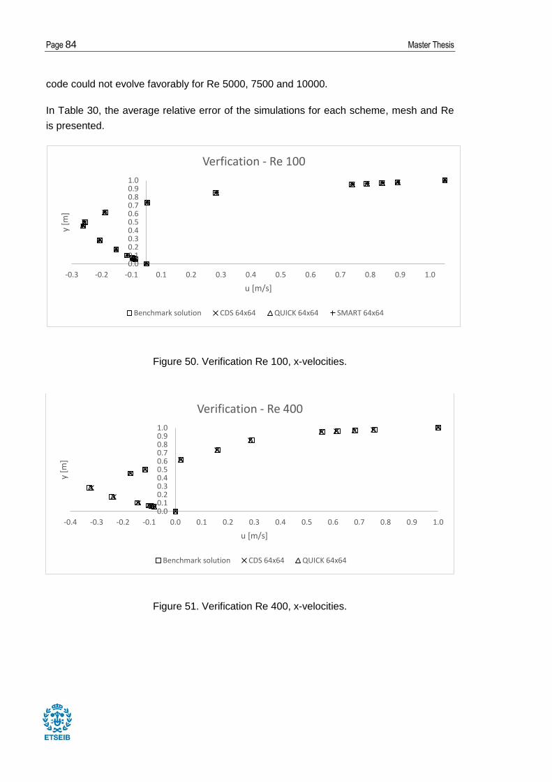
Page 84 Master Thesis
code could not evolve favorably for Re 5000, 7500 and 10000.
In Table 30, the average relative error of the simulations for each scheme, mesh and Re
is presented.
Figure 50. Verification Re 100, x-velocities.
Figure 51. Verification Re 400, x-velocities.
0.0 0.1 0.2 0.3 0.4 0.5 0.6 0.7 0.8 0.9 1.0
-0.3 -0.2 -0.1 0.1 0.2 0.3 0.4 0.5 0.6 0.7 0.8 0.9 1.0
y [m
]
u [m/s]
Verfication - Re 100
Benchmark solution CDS 64x64 QUICK 64x64 SMART 64x64
0.0 0.1 0.2 0.3 0.4 0.5 0.6 0.7 0.8 0.9 1.0
-0.4 -0.3 -0.2 -0.1 0.0 0.1 0.2 0.3 0.4 0.5 0.6 0.7 0.8 0.9 1.0
y [m
]
u [m/s]
Verification - Re 400
Benchmark solution CDS 64x64 QUICK 64x64
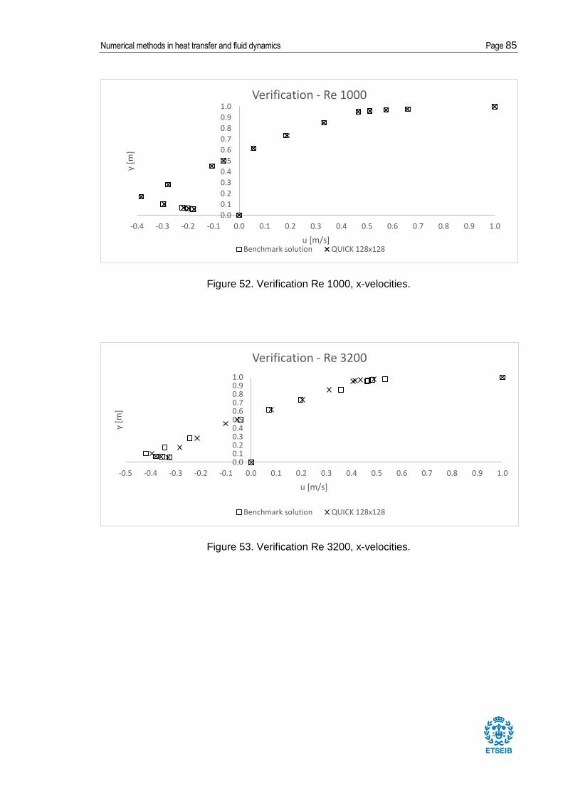
Numerical methods in heat transfer and fluid dynamics Page 85
Figure 52. Verification Re 1000, x-velocities.
Figure 53. Verification Re 3200, x-velocities.
0.0
0.1
0.2
0.3
0.4
0.5
0.6
0.7
0.8
0.9
1.0
-0.4 -0.3 -0.2 -0.1 0.0 0.1 0.2 0.3 0.4 0.5 0.6 0.7 0.8 0.9 1.0
y [m
]
u [m/s]
Verification - Re 1000
Benchmark solution QUICK 128x128
0.0 0.1 0.2 0.3 0.4 0.5 0.6 0.7 0.8 0.9 1.0
-0.5 -0.4 -0.3 -0.2 -0.1 0.0 0.1 0.2 0.3 0.4 0.5 0.6 0.7 0.8 0.9 1.0
y [m
]
u [m/s]
Verification - Re 3200
Benchmark solution QUICK 128x128
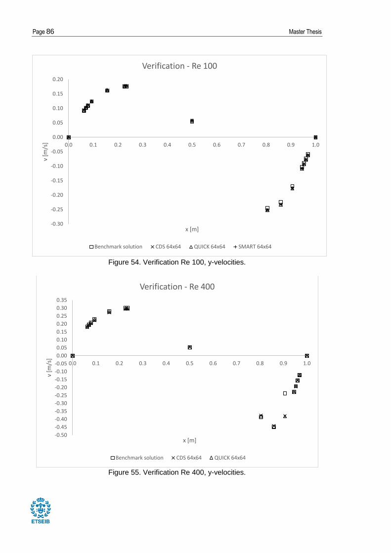
Page 86 Master Thesis
Figure 54. Verification Re 100, y-velocities.
Figure 55. Verification Re 400, y-velocities.
-0.30
-0.25
-0.20
-0.15
-0.10
-0.05
0.00
0.05
0.10
0.15
0.20
0.0 0.1 0.2 0.3 0.4 0.5 0.6 0.7 0.8 0.9 1.0
v [m
/s]
x [m]
Verification - Re 100
Benchmark solution CDS 64x64 QUICK 64x64 SMART 64x64
-0.50
-0.45
-0.40
-0.35
-0.30
-0.25
-0.20
-0.15
-0.10
-0.05
0.00
0.05
0.10
0.15
0.20
0.25
0.30
0.35
0.0 0.1 0.2 0.3 0.4 0.5 0.6 0.7 0.8 0.9 1.0
v [m
/s]
x [m]
Verification - Re 400
Benchmark solution CDS 64x64 QUICK 64x64
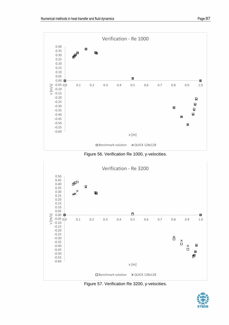
Numerical methods in heat transfer and fluid dynamics Page 87
Figure 56. Verification Re 1000, y-velocities.
Figure 57. Verification Re 3200, y-velocities.
-0.60 -0.55 -0.50 -0.45 -0.40 -0.35 -0.30 -0.25 -0.20 -0.15 -0.10 -0.05 0.00 0.05 0.10 0.15 0.20 0.25 0.30 0.35 0.40
0.0 0.1 0.2 0.3 0.4 0.5 0.6 0.7 0.8 0.9 1.0
v [m
/s]
x [m]
Verification - Re 1000
Benchmark solution QUICK 128x128
-0.60 -0.55 -0.50 -0.45 -0.40 -0.35 -0.30 -0.25 -0.20 -0.15 -0.10 -0.05 0.00 0.05 0.10 0.15 0.20 0.25 0.30 0.35 0.40 0.45 0.50
0.0 0.1 0.2 0.3 0.4 0.5 0.6 0.7 0.8 0.9 1.0
v [m
/s]
x [m]
Verification - Re 3200
Benchmark solution QUICK 128x128
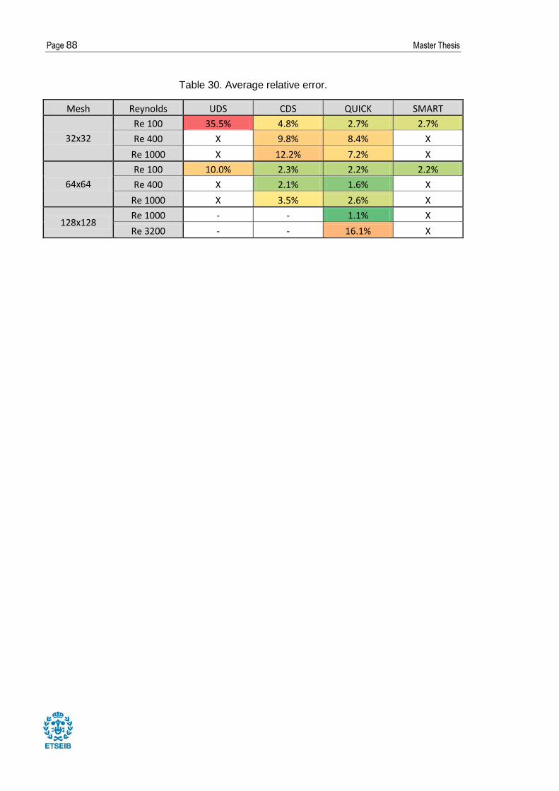
Page 88 Master Thesis
Table 30. Average relative error.
Mesh Reynolds UDS CDS QUICK SMART
32x32
Re 100 35.5% 4.8% 2.7% 2.7%
Re 400 X 9.8% 8.4% X
Re 1000 X 12.2% 7.2% X
64x64
Re 100 10.0% 2.3% 2.2% 2.2%
Re 400 X 2.1% 1.6% X
Re 1000 X 3.5% 2.6% X
128x128 Re 1000 - - 1.1% X
Re 3200 - - 16.1% X

Numerical methods in heat transfer and fluid dynamics Page 89
Table 31 to Table 36 show the results obtained for Re 100, 400, 1000 and 3200 are
registered using different convective schemes and mesh sizes.
Table 31. Results for Re 100 (1/2)
Re = 100 UDS 32x32 CDS 32x32 QUICK 32x32 SMART 32x32
y [m] u [m/s] u [m/s] Error u [m/s] Error u [m/s] Error u [m/s] Error
1.0000 1.00000 1.00000 - 1.00000 - 1.00000 - 1.00000 -
0.9766 0.84123
0.9688 0.78871 0.67026 15.0% 0.78977 0.1% 13.1% 0.78619 0.3%
0.9609 0.73722
0.9531 0.68717 0.67026 2.5% 0.68526 0.3% 0.68542 0.3% 0.68538 0.3%
0.8516 0.23151
0.7344 0.00332 -0.01109 434.0% 0.00152 54.2% 0.00317 4.5% 0.00301 9.3%
0.6172 -0.13641
0.5000 -0.20581 -0.19315 6.2% -0.20392 0.9% -0.20598 0.1% -0.20608 0.1%
0.4531 -0.21090 -0.19299 8.5% -0.20890 0.9% -0.21048 0.2% -0.21060 0.1%
0.2813 -0.15662 -0.14576 6.9% -0.15604 0.4% -0.15536 0.8% -0.15522 0.9%
0.1719 -0.10150 -0.09162 9.7% -0.10045 1.0% -0.10060 0.9% -0.10041 1.1%
0.1016 -0.06434
0.0703 -0.04775
0.0625 -0.04192 -0.04739 13.0% -0.04121 1.7% -0.04175 0.4% -0.04165 0.6%
0.0547 -0.03717
0.0000 0.00000 0.00000 - 0.00000 - 0.00000 - 0.00000 -
x [m] v [m/s] v [m/s] Error v [m/s] Error v [m/s] Error v [m/s] Error
1.0000 0.00000 0.00000 - 0.00000 - 0.00000 - 0.00000 -
0.9688 -0.05906 -0.02966 49.8% -0.06220 5.3% -0.06160 4.3% -0.06150 4.1%
0.9609 -0.07391
0.9531 -0.08864 -0.08935 0.8% -0.09470 6.8% -0.09328 5.2% -0.09311 5.0%
0.9453 -0.10313
0.9063 -0.16914 -0.14225 15.9% -0.17605 4.1% -0.17690 4.6% -0.17651 4.4%
0.8594 -0.22445 -0.20750 7.6% -0.23276 3.7% -0.23283 3.7% -0.23222 3.5%
0.8047 -0.24533
0.5000 0.05454 0.04798 12.0% 0.05732 5.1% 0.05771 5.8% 0.05758 5.6%
0.2344 0.17527 0.16569 5.5% 0.17521 0.0% 0.17619 0.5% 0.17612 0.5%
0.2266 0.17507
0.1563 0.16077 0.14708 8.5% 0.15986 0.6% 0.16171 0.6% 0.16164 0.5%
0.0938 0.12317 0.10410 15.5% 0.12226 0.7% 0.12430 0.9% 0.12426 0.9%
0.0781 0.10890 0.10410 4.4% 0.10920 0.3% 0.11005 1.1% 0.10999 1.0%
0.0703 0.10091
0.0625 0.09233 0.07031 23.8% 0.09161 0.8% 0.09366 1.4% 0.09360 1.4%
0.0000 0.00000 0.00000 - 0.00000 - 0.00000 - 0.00000 -
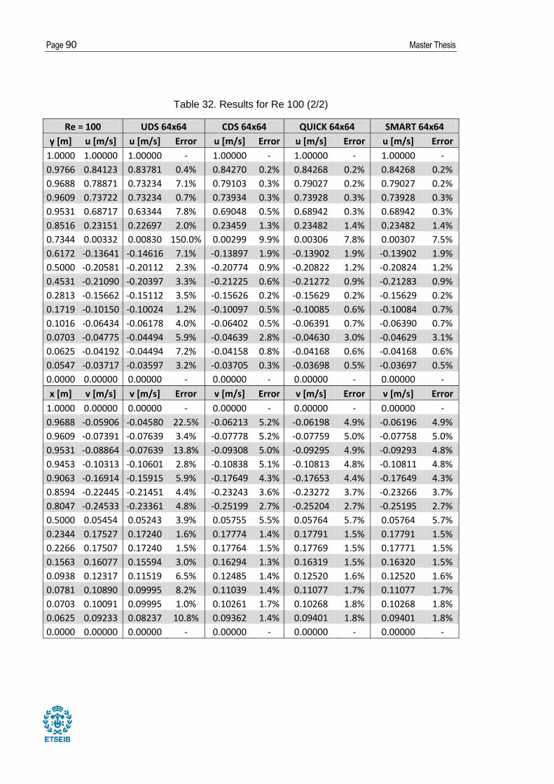
Page 90 Master Thesis
Table 32. Results for Re 100 (2/2)
Re = 100 UDS 64x64 CDS 64x64 QUICK 64x64 SMART 64x64
y [m] u [m/s] u [m/s] Error u [m/s] Error u [m/s] Error u [m/s] Error
1.0000 1.00000 1.00000 - 1.00000 - 1.00000 - 1.00000 -
0.9766 0.84123 0.83781 0.4% 0.84270 0.2% 0.84268 0.2% 0.84268 0.2%
0.9688 0.78871 0.73234 7.1% 0.79103 0.3% 0.79027 0.2% 0.79027 0.2%
0.9609 0.73722 0.73234 0.7% 0.73934 0.3% 0.73928 0.3% 0.73928 0.3%
0.9531 0.68717 0.63344 7.8% 0.69048 0.5% 0.68942 0.3% 0.68942 0.3%
0.8516 0.23151 0.22697 2.0% 0.23459 1.3% 0.23482 1.4% 0.23482 1.4%
0.7344 0.00332 0.00830 150.0% 0.00299 9.9% 0.00306 7.8% 0.00307 7.5%
0.6172 -0.13641 -0.14616 7.1% -0.13897 1.9% -0.13902 1.9% -0.13902 1.9%
0.5000 -0.20581 -0.20112 2.3% -0.20774 0.9% -0.20822 1.2% -0.20824 1.2%
0.4531 -0.21090 -0.20397 3.3% -0.21225 0.6% -0.21272 0.9% -0.21283 0.9%
0.2813 -0.15662 -0.15112 3.5% -0.15626 0.2% -0.15629 0.2% -0.15629 0.2%
0.1719 -0.10150 -0.10024 1.2% -0.10097 0.5% -0.10085 0.6% -0.10084 0.7%
0.1016 -0.06434 -0.06178 4.0% -0.06402 0.5% -0.06391 0.7% -0.06390 0.7%
0.0703 -0.04775 -0.04494 5.9% -0.04639 2.8% -0.04630 3.0% -0.04629 3.1%
0.0625 -0.04192 -0.04494 7.2% -0.04158 0.8% -0.04168 0.6% -0.04168 0.6%
0.0547 -0.03717 -0.03597 3.2% -0.03705 0.3% -0.03698 0.5% -0.03697 0.5%
0.0000 0.00000 0.00000 - 0.00000 - 0.00000 - 0.00000 -
x [m] v [m/s] v [m/s] Error v [m/s] Error v [m/s] Error v [m/s] Error
1.0000 0.00000 0.00000 - 0.00000 - 0.00000 - 0.00000 -
0.9688 -0.05906 -0.04580 22.5% -0.06213 5.2% -0.06198 4.9% -0.06196 4.9%
0.9609 -0.07391 -0.07639 3.4% -0.07778 5.2% -0.07759 5.0% -0.07758 5.0%
0.9531 -0.08864 -0.07639 13.8% -0.09308 5.0% -0.09295 4.9% -0.09293 4.8%
0.9453 -0.10313 -0.10601 2.8% -0.10838 5.1% -0.10813 4.8% -0.10811 4.8%
0.9063 -0.16914 -0.15915 5.9% -0.17649 4.3% -0.17653 4.4% -0.17649 4.3%
0.8594 -0.22445 -0.21451 4.4% -0.23243 3.6% -0.23272 3.7% -0.23266 3.7%
0.8047 -0.24533 -0.23361 4.8% -0.25199 2.7% -0.25204 2.7% -0.25195 2.7%
0.5000 0.05454 0.05243 3.9% 0.05755 5.5% 0.05764 5.7% 0.05764 5.7%
0.2344 0.17527 0.17240 1.6% 0.17774 1.4% 0.17791 1.5% 0.17791 1.5%
0.2266 0.17507 0.17240 1.5% 0.17764 1.5% 0.17769 1.5% 0.17771 1.5%
0.1563 0.16077 0.15594 3.0% 0.16294 1.3% 0.16319 1.5% 0.16320 1.5%
0.0938 0.12317 0.11519 6.5% 0.12485 1.4% 0.12520 1.6% 0.12520 1.6%
0.0781 0.10890 0.09995 8.2% 0.11039 1.4% 0.11077 1.7% 0.11077 1.7%
0.0703 0.10091 0.09995 1.0% 0.10261 1.7% 0.10268 1.8% 0.10268 1.8%
0.0625 0.09233 0.08237 10.8% 0.09362 1.4% 0.09401 1.8% 0.09401 1.8%
0.0000 0.00000 0.00000 - 0.00000 - 0.00000 - 0.00000 -
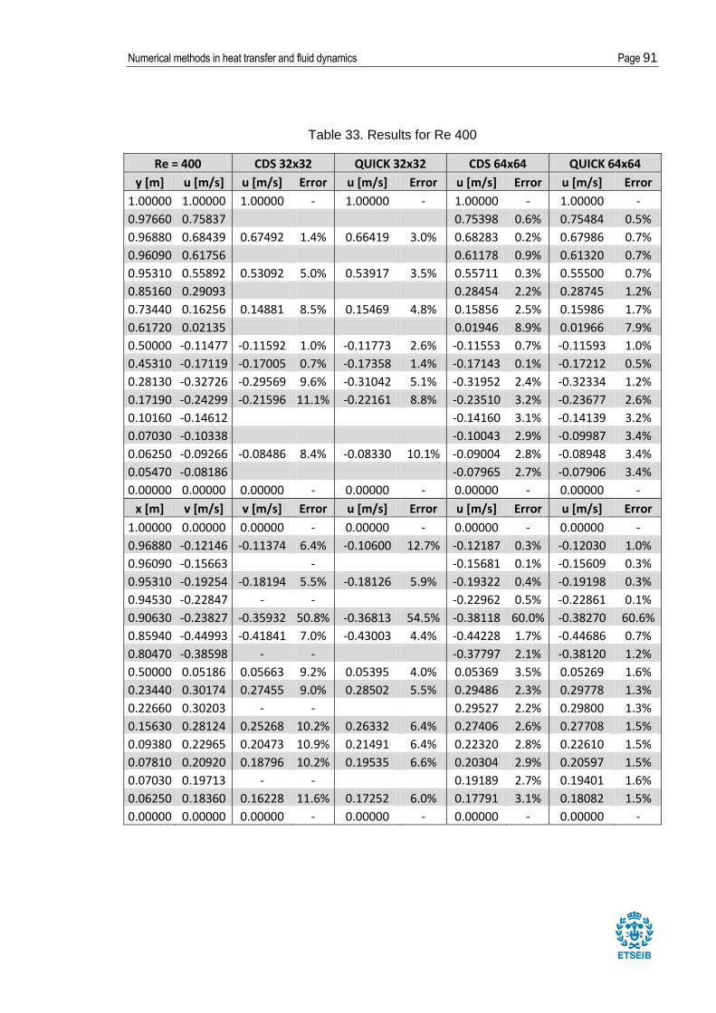
Numerical methods in heat transfer and fluid dynamics Page 91
Table 33. Results for Re 400
Re = 400 CDS 32x32 QUICK 32x32 CDS 64x64 QUICK 64x64
y [m] u [m/s] u [m/s] Error u [m/s] Error u [m/s] Error u [m/s] Error
1.00000 1.00000 1.00000 - 1.00000 - 1.00000 - 1.00000 -
0.97660 0.75837 0.75398 0.6% 0.75484 0.5%
0.96880 0.68439 0.67492 1.4% 0.66419 3.0% 0.68283 0.2% 0.67986 0.7%
0.96090 0.61756 0.61178 0.9% 0.61320 0.7%
0.95310 0.55892 0.53092 5.0% 0.53917 3.5% 0.55711 0.3% 0.55500 0.7%
0.85160 0.29093 0.28454 2.2% 0.28745 1.2%
0.73440 0.16256 0.14881 8.5% 0.15469 4.8% 0.15856 2.5% 0.15986 1.7%
0.61720 0.02135 0.01946 8.9% 0.01966 7.9%
0.50000 -0.11477 -0.11592 1.0% -0.11773 2.6% -0.11553 0.7% -0.11593 1.0%
0.45310 -0.17119 -0.17005 0.7% -0.17358 1.4% -0.17143 0.1% -0.17212 0.5%
0.28130 -0.32726 -0.29569 9.6% -0.31042 5.1% -0.31952 2.4% -0.32334 1.2%
0.17190 -0.24299 -0.21596 11.1% -0.22161 8.8% -0.23510 3.2% -0.23677 2.6%
0.10160 -0.14612
-0.14160 3.1% -0.14139 3.2%
0.07030 -0.10338 -0.10043 2.9% -0.09987 3.4%
0.06250 -0.09266 -0.08486 8.4% -0.08330 10.1% -0.09004 2.8% -0.08948 3.4%
0.05470 -0.08186 -0.07965 2.7% -0.07906 3.4%
0.00000 0.00000 0.00000 - 0.00000 - 0.00000 - 0.00000 -
x [m] v [m/s] v [m/s] Error u [m/s] Error u [m/s] Error u [m/s] Error
1.00000 0.00000 0.00000 - 0.00000 - 0.00000 - 0.00000 -
0.96880 -0.12146 -0.11374 6.4% -0.10600 12.7% -0.12187 0.3% -0.12030 1.0%
0.96090 -0.15663 -
-0.15681 0.1% -0.15609 0.3%
0.95310 -0.19254 -0.18194 5.5% -0.18126 5.9% -0.19322 0.4% -0.19198 0.3%
0.94530 -0.22847 - -
-0.22962 0.5% -0.22861 0.1%
0.90630 -0.23827 -0.35932 50.8% -0.36813 54.5% -0.38118 60.0% -0.38270 60.6%
0.85940 -0.44993 -0.41841 7.0% -0.43003 4.4% -0.44228 1.7% -0.44686 0.7%
0.80470 -0.38598 - - -0.37797 2.1% -0.38120 1.2%
0.50000 0.05186 0.05663 9.2% 0.05395 4.0% 0.05369 3.5% 0.05269 1.6%
0.23440 0.30174 0.27455 9.0% 0.28502 5.5% 0.29486 2.3% 0.29778 1.3%
0.22660 0.30203 - -
0.29527 2.2% 0.29800 1.3%
0.15630 0.28124 0.25268 10.2% 0.26332 6.4% 0.27406 2.6% 0.27708 1.5%
0.09380 0.22965 0.20473 10.9% 0.21491 6.4% 0.22320 2.8% 0.22610 1.5%
0.07810 0.20920 0.18796 10.2% 0.19535 6.6% 0.20304 2.9% 0.20597 1.5%
0.07030 0.19713 - -
0.19189 2.7% 0.19401 1.6%
0.06250 0.18360 0.16228 11.6% 0.17252 6.0% 0.17791 3.1% 0.18082 1.5%
0.00000 0.00000 0.00000 - 0.00000 - 0.00000 - 0.00000 -

Page 92 Master Thesis
Table 34. Results for Re 1000 (1/2)
Re = 1000 CDS 32x32 QUICK 32x32 CDS 64x64 QUICK 64x64
y [m] u [m/s] u [m/s] Error u [m/s] Error u [m/s] Error u [m/s] Error
1.00000 1.00000 1.00000 - 1.00000 - 1.00000 - 1.00000 -
0.97660 0.65928 0.64266 2.5% 0.64627 2.0%
0.96880 0.57492 0.55858 2.8% 0.55325 3.8% 0.56824 1.2% 0.56421 1.9%
0.96090 0.51117 0.49382 3.4% 0.50032 2.1%
0.95310 0.46604 0.40871 12.3% 0.43880 5.8% 0.45627 2.1% 0.45851 1.6%
0.85160 0.33304 0.31969 4.0% 0.32548 2.3%
0.73440 0.18179 0.16104 11.4% 0.17605 3.2% 0.18030 0.8% 0.18254 0.4%
0.61720 0.05702 0.05365 5.9% 0.05421 4.9%
0.50000 -0.06080 -0.05821 4.3% -0.06341 4.3% -0.06140 1.0% -0.06210 2.1%
0.45310 -0.10648 -0.09805 7.9% -0.10708 0.6% -0.10573 0.7% -0.10699 0.5%
0.28130 -0.27805 -0.25322 8.9% -0.27602 0.7% -0.27181 2.2% -0.27577 0.8%
0.17190 -0.38289 -0.31525 17.7% -0.34588 9.7% -0.36408 4.9% -0.37324 2.5%
0.10160 -0.29730
-0.27832 6.4% -0.28109 5.5%
0.07030 -0.22220 -0.20796 6.4% -0.20732 6.7%
0.06250 -0.20196 -0.16281 19.4% -0.16295 19.3% -0.18894 6.4% -0.18792 7.0%
0.05470 -0.18109 -0.16992 6.2% -0.16821 7.1%
0.00000 0.00000 0.00000 - 0.00000 - 0.00000 - 0.00000 -
x [m] v [m/s] v [m/s] Error v [m/s] Error v [m/s] Error v [m/s] Error
1.00000 0.00000 0.00000 - 0.00000 - 0.00000 - 0.00000 -
0.96880 -0.21388 -0.19348 9.5% -0.17214 19.5% -0.21199 0.9% -0.20777 2.9%
0.96090 -0.27669 - -
-0.27582 0.3% -0.27322 1.3%
0.95310 -0.33714 -0.32666 3.1% -0.32635 3.2% -0.33315 1.2% -0.33247 1.4%
0.94530 -0.39188 - -
-0.39049 0.4% -0.38905 0.7%
0.90630 -0.51550 -0.43324 16.0% -0.48020 6.8% -0.49473 4.0% -0.50835 1.4%
0.85940 -0.42665 -0.37420 12.3% -0.40270 5.6% -0.41148 3.6% -0.41863 1.9%
0.80470 -0.31966 - - -0.30813 3.6% -0.31222 2.3%
0.50000 0.02526 0.02720 7.7% 0.02453 2.9% 0.02656 5.1% 0.02540 0.6%
0.23440 0.32235 0.28322 12.1% 0.30420 5.6% 0.31230 3.1% 0.31632 1.9%
0.22660 0.33075 - -
0.32020 3.2% 0.32437 1.9%
0.15630 0.37095 0.30600 17.5% 0.33942 8.5% 0.35355 4.7% 0.36182 2.5%
0.09380 0.32627 0.26442 19.0% 0.29426 9.8% 0.30947 5.1% 0.31728 2.8%
0.07810 0.30353 0.24760 18.4% 0.27256 10.2% 0.28767 5.2% 0.29520 2.7%
0.07030 0.29012 - -
0.27559 5.0% 0.28191 2.8%
0.06250 0.27485 0.22031 19.8% 0.24970 9.2% 0.25987 5.5% 0.26742 2.7%
0.00000 0.00000 0.00000 - 0.00000 - 0.00000 - 0.00000 -
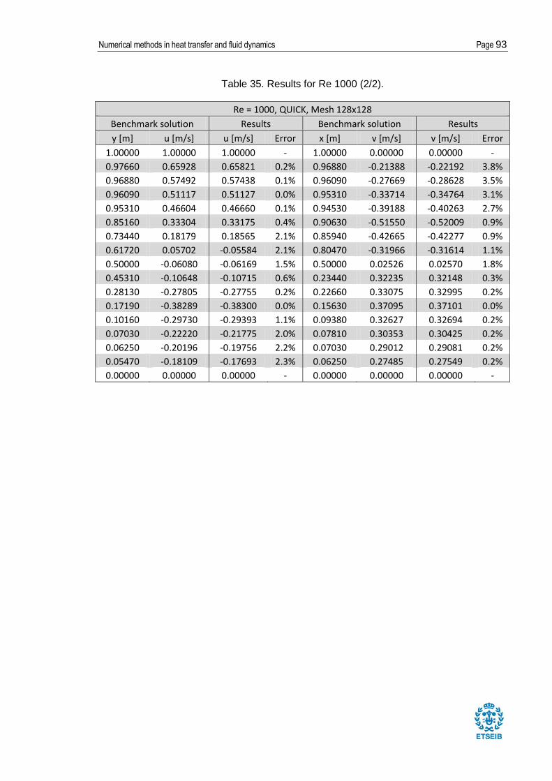
Numerical methods in heat transfer and fluid dynamics Page 93
Table 35. Results for Re 1000 (2/2).
Re = 1000, QUICK, Mesh 128x128
Benchmark solution Results Benchmark solution Results
y [m] u [m/s] u [m/s] Error x [m] v [m/s] v [m/s] Error
1.00000 1.00000 1.00000 - 1.00000 0.00000 0.00000 -
0.97660 0.65928 0.65821 0.2% 0.96880 -0.21388 -0.22192 3.8%
0.96880 0.57492 0.57438 0.1% 0.96090 -0.27669 -0.28628 3.5%
0.96090 0.51117 0.51127 0.0% 0.95310 -0.33714 -0.34764 3.1%
0.95310 0.46604 0.46660 0.1% 0.94530 -0.39188 -0.40263 2.7%
0.85160 0.33304 0.33175 0.4% 0.90630 -0.51550 -0.52009 0.9%
0.73440 0.18179 0.18565 2.1% 0.85940 -0.42665 -0.42277 0.9%
0.61720 0.05702 -0.05584 2.1% 0.80470 -0.31966 -0.31614 1.1%
0.50000 -0.06080 -0.06169 1.5% 0.50000 0.02526 0.02570 1.8%
0.45310 -0.10648 -0.10715 0.6% 0.23440 0.32235 0.32148 0.3%
0.28130 -0.27805 -0.27755 0.2% 0.22660 0.33075 0.32995 0.2%
0.17190 -0.38289 -0.38300 0.0% 0.15630 0.37095 0.37101 0.0%
0.10160 -0.29730 -0.29393 1.1% 0.09380 0.32627 0.32694 0.2%
0.07030 -0.22220 -0.21775 2.0% 0.07810 0.30353 0.30425 0.2%
0.06250 -0.20196 -0.19756 2.2% 0.07030 0.29012 0.29081 0.2%
0.05470 -0.18109 -0.17693 2.3% 0.06250 0.27485 0.27549 0.2%
0.00000 0.00000 0.00000 - 0.00000 0.00000 0.00000 -
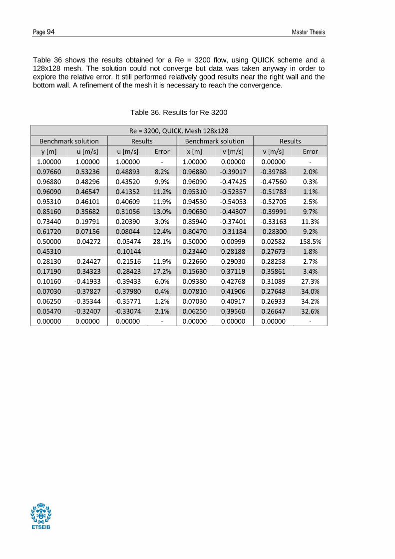
Page 94 Master Thesis
Table 36 shows the results obtained for a Re = 3200 flow, using QUICK scheme and a 128x128 mesh. The solution could not converge but data was taken anyway in order to explore the relative error. It still performed relatively good results near the right wall and the bottom wall. A refinement of the mesh it is necessary to reach the convergence.
Table 36. Results for Re 3200
Re = 3200, QUICK, Mesh 128x128
Benchmark solution Results Benchmark solution Results
y [m] u [m/s] u [m/s] Error x [m] v [m/s] v [m/s] Error
1.00000 1.00000 1.00000 - 1.00000 0.00000 0.00000 -
0.97660 0.53236 0.48893 8.2% 0.96880 -0.39017 -0.39788 2.0%
0.96880 0.48296 0.43520 9.9% 0.96090 -0.47425 -0.47560 0.3%
0.96090 0.46547 0.41352 11.2% 0.95310 -0.52357 -0.51783 1.1%
0.95310 0.46101 0.40609 11.9% 0.94530 -0.54053 -0.52705 2.5%
0.85160 0.35682 0.31056 13.0% 0.90630 -0.44307 -0.39991 9.7%
0.73440 0.19791 0.20390 3.0% 0.85940 -0.37401 -0.33163 11.3%
0.61720 0.07156 0.08044 12.4% 0.80470 -0.31184 -0.28300 9.2%
0.50000 -0.04272 -0.05474 28.1% 0.50000 0.00999 0.02582 158.5%
0.45310 -0.10144 0.23440 0.28188 0.27673 1.8%
0.28130 -0.24427 -0.21516 11.9% 0.22660 0.29030 0.28258 2.7%
0.17190 -0.34323 -0.28423 17.2% 0.15630 0.37119 0.35861 3.4%
0.10160 -0.41933 -0.39433 6.0% 0.09380 0.42768 0.31089 27.3%
0.07030 -0.37827 -0.37980 0.4% 0.07810 0.41906 0.27648 34.0%
0.06250 -0.35344 -0.35771 1.2% 0.07030 0.40917 0.26933 34.2%
0.05470 -0.32407 -0.33074 2.1% 0.06250 0.39560 0.26647 32.6%
0.00000 0.00000 0.00000 - 0.00000 0.00000 0.00000 -
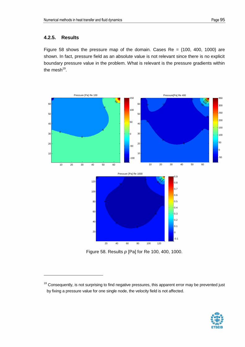
Numerical methods in heat transfer and fluid dynamics Page 95
4.2.5. Results
Figure 58 shows the pressure map of the domain. Cases Re = {100, 400, 1000} are
shown. In fact, pressure field as an absolute value is not relevant since there is no explicit
boundary pressure value in the problem. What is relevant is the pressure gradients within
the mesh19.
Figure 58. Results p [Pa] for Re 100, 400, 1000.
19 Consequently, is not surprising to find negative pressures, this apparent error may be prevented just
by fixing a pressure value for one single node, the velocity field is not affected.
0
0
0
0
50
Pressure [Pa] Re 100
10 20 30 40 50 60
10
20
30
40
50
60
-100
-50
0
50
100
150
0
0
0
0
0
0
0
0 50
100
150200
Pressure[Pa] Re 400
10 20 30 40 50 60
10
20
30
40
50
60
-50
0
50
100
150
200
250
300
350
0
0
0
0
0
0
0
0.1
0.20.3
Pressure [Pa] Re 1000
20 40 60 80 100 120
20
40
60
80
100
120
-0.1
0
0.1
0.2
0.3
0.4
0.5
0.6
0.7
0.8
0.9
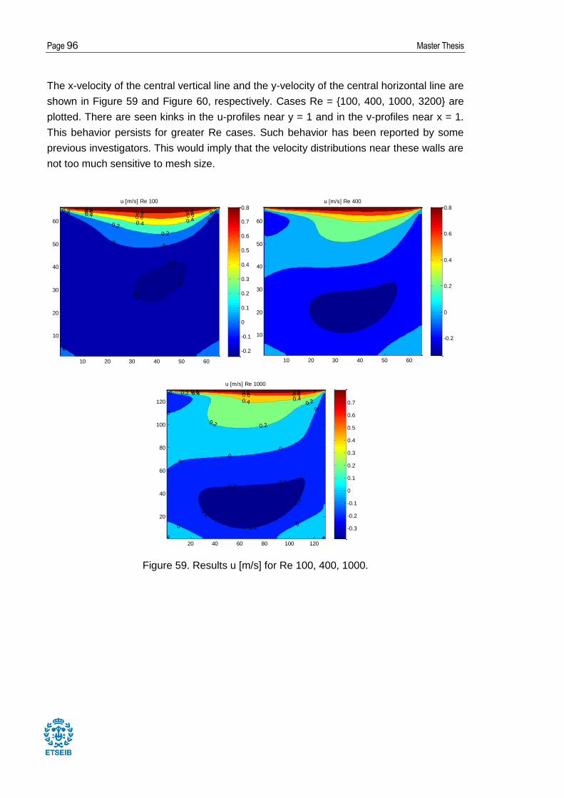
Page 96 Master Thesis
The x-velocity of the central vertical line and the y-velocity of the central horizontal line are
shown in Figure 59 and Figure 60, respectively. Cases Re = {100, 400, 1000, 3200} are
plotted. There are seen kinks in the u-profiles near y = 1 and in the v-profiles near x = 1.
This behavior persists for greater Re cases. Such behavior has been reported by some
previous investigators. This would imply that the velocity distributions near these walls are
not too much sensitive to mesh size.
Figure 59. Results u [m/s] for Re 100, 400, 1000.
0
0
00
0 0.2
0.2
0.2
0.2
0.40.4
0.4
-0.2
-0.2
-0.2
0.60.60.6 0.80.80.8
u [m/s] Re 100
10 20 30 40 50 60
10
20
30
40
50
60
-0.2
-0.1
0
0.1
0.2
0.3
0.4
0.5
0.6
0.7
0.8u [m/s] Re 400
10 20 30 40 50 60
10
20
30
40
50
60
-0.2
0
0.2
0.4
0.6
0.8
0 0
0
0
00
-0.2-0.2
-0.2
-0.2
-0.2
0.2
0.20.2
0.20.40.4
0.4 0.60.60.6
0
0 0.80.80.8
0
u [m/s] Re 1000
20 40 60 80 100 120
20
40
60
80
100
120
-0.3
-0.2
-0.1
0
0.1
0.2
0.3
0.4
0.5
0.6
0.7
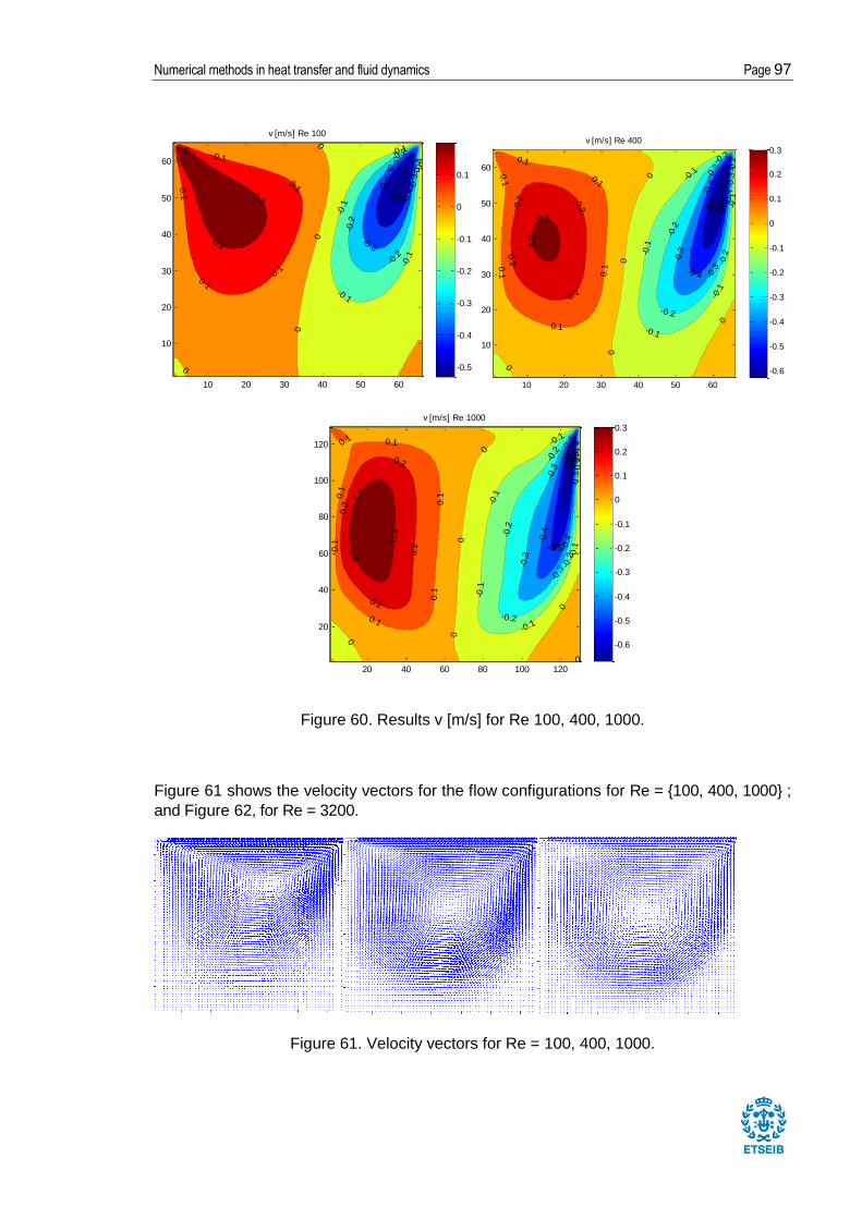
Numerical methods in heat transfer and fluid dynamics Page 97
Figure 60. Results v [m/s] for Re 100, 400, 1000.
Figure 61 shows the velocity vectors for the flow configurations for Re = {100, 400, 1000} ;
and Figure 62, for Re = 3200.
Figure 61. Velocity vectors for Re = 100, 400, 1000.
0
0
0
0.1
0.1
0.1
0.1
0.1
-0.1
-0.1
-0.1
-0.1
-0.1-0.2
-0.2
-0.2
-0.2
0.2
0.2
0.2
0.2
-0.3
-0.3
-0.3
-0.4
-0.4
-0.5
0
v [m/s] Re 100
10 20 30 40 50 60
10
20
30
40
50
60
-0.5
-0.4
-0.3
-0.2
-0.1
0
0.1 0
0
0
0
0.1
0.1
0.1
0.1
0.1
0.1 -0
.1
-0.1
-0.1
-0.1
-0.1
0.2 0
.2
0.2
0.2
-0.2
-0.2
-0.2
-0.2
-0.2
-0.3
-0.3
-0.3
-0.3
-0.4
-0.4
-0.4
-0.5
-0.5
0.3
0.3
0
-0.6
v [m/s] Re 400
10 20 30 40 50 60
10
20
30
40
50
60
-0.6
-0.5
-0.4
-0.3
-0.2
-0.1
0
0.1
0.2
0.3
00
0
0
0.1
0.10.1
0.1
0.1
0.1
-0.1
-0.1
-0.1
-0.1
-0.1
-0.1
0.2
0.2
0.2
0.2
-0.2
-0.2
-0.2
-0.2
-0.2
-0.3
-0.3
-0.3
-0.3
0.3
0.3
0.3
-0.4
-0.4
-0.4
-0.4
-0.5
-0.5
-0.5
0
-0.6
-0.6
0.1
0
v [m/s] Re 1000
20 40 60 80 100 120
20
40
60
80
100
120
-0.6
-0.5
-0.4
-0.3
-0.2
-0.1
0
0.1
0.2
0.3

Page 98 Master Thesis
Figure 62. Velocity vectors for Re = 3200.
0 20 40 60 80 100 120 1400
20
40
60
80
100
120
140
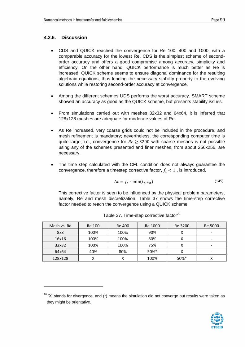
Numerical methods in heat transfer and fluid dynamics Page 99
4.2.6. Discussion
CDS and QUICK reached the convergence for Re 100. 400 and 1000, with a
comparable accuracy for the lowest Re. CDS is the simplest scheme of second-
order accuracy and offers a good compromise among accuracy, simplicity and
efficiency. On the other hand, QUICK performance is much better as Re is
increased. QUICK scheme seems to ensure diagonal dominance for the resulting
algebraic equations, thus lending the necessary stability property to the evolving
solutions while restoring second-order accuracy at convergence.
Among the different schemes UDS performs the worst accuracy. SMART scheme
showed an accuracy as good as the QUICK scheme, but presents stability issues.
From simulations carried out with meshes 32x32 and 64x64, it is inferred that
128x128 meshes are adequate for moderate values of Re.
As Re increased, very coarse grids could not be included in the procedure, and
mesh refinement is mandatory; nevertheless, the corresponding computer time is
quite large, i.e., convergence for with coarse meshes is not possible
using any of the schemes presented and finer meshes, from about 256x256, are
necessary.
The time step calculated with the CFL condition does not always guarantee the
convergence, therefore a timestep corrective factor, , is introduced.
(145)
This corrective factor is seen to be influenced by the physical problem parameters,
namely, Re and mesh discretization. Table 37 shows the time-step corrective
factor needed to reach the convergence using a QUICK scheme.
Table 37. Time-step corrective factor20
Mesh vs. Re Re 100 Re 400 Re 1000 Re 3200 Re 5000
8x8 100% 100% 90% X -
16x16 100% 100% 80% X -
32x32 100% 100% 75% X -
64x64 40% 80% 50%* X -
128x128 X X 100% 50%* X
20 ‘X’ stands for divergence, and (*) means the simulation did not converge but results were taken as
they might be orientative.
Page 100 Master Thesis
A pressure relaxation factor, , was used in all the cases to achieve the
pressure field convergence.
The relative error is significant near the walls, this may be solved refining the mesh
or using an irregular mesh with higher density of CVs near the walls (as seen in
Chapter 5).
It is interesting to study the influence of parameters and for a given Re. For
example, for a , the computing time is much lower for a set of and
than for a set of and .
Difficulties have been experienced with the convergence for high Re, mainly due to
the limits of the computer processor used. The size of the computational mesh
employed must be increased and the use of a workstation would be much helpful.

Numerical methods in heat transfer and fluid dynamics Page 101
Conclusions
Heat conduction methods
An understanding of the heat conduction solution methodology is essential. To be
able to see the similarities between transfer of momentum and transfer of heat and to
regard velocity as, in some ways, analogous to temperature, is a great conceptual
help. The use of heat conduction as a building block in the fluid-flow calculation
scheme reinforces this conceptual unity.
The TDMA is a very powerful and convenient equation solver whenever the
algebraic equations can be represented with the generic conservation equation. In
the ‘Four materials problem’ it was noticed that the TDMA requires time
proportional to N, the number of CVs, rather than to N2 or N3.
The convection-diffusion equation
Many of the features commonly encountered in practical convection-diffusion
problems were present in the Smith-Hutton problem. The streamline pattern is fairly
complicated, exhibiting a large degree of curvature (a general feature of recirculating
flows), and the transported variable displays a rapid change over a small distance
within the flow (possibly as a consequence of a source, the mixing of two streams of
different temperature, etc.).
According to the relaxation factor analysis applied to the Smith-Hutton problem, it
has been determined that there are no general rules for choosing the best value of
a relaxation factor. The optimum value depends upon many factors, such as the
nature of the problem, the number of grid points, the grid spacing, and the iterative
process used. Suitable values of were found from exploratory computations for
the given problem.
Finding an appropriate relaxation factor for high-order schemes is in some cases a
necessary requirement and shall be faced by first exploring the behavior of the
system in coarse meshes and progressively refining them. The optimal relaxation
factor will depend on the numerical, physical and geometrical factors of the problem.
The study of different schemes for the discretization of the convective term in the
Page 102 Master Thesis
convection-diffusion equation evidenced that:
o There does not appear to be a perfect scheme. On regular coarse meshes,
all the methods submitted showed evidence of false diffusion or spatial
oscillations or some combination of the above.
o UDS is characterized by false diffusion, which completely swamps the real
diffusion at high Peclet numbers. The scheme gives physically plausible
results, but on practical meshes it appears to be impossible to make accurate
predictions at high Pe.
o CDS tend to give false spatial oscillations when the mesh refinement is
insufficient to resolve variations of the dependent variable that occur in the
problem. If the mesh is refined an accurate solution will result. This behavior
could be considered an advantage, given that the oscillations are a warning
that the grid is insufficient to give an accurate solution.
o High-order schemes yield performances on coarse meshes that represent a
compromise between diffusive and spatial oscillation errors. It is noteworthy,
however, that these schemes do not always give good results at low Pe, a
matter of some concern if calculating a complex flow containing regimes of
differing Peclet numbers.
Incompressible flow method
The robustness of the FSM has been demonstrated using the model problem ‘Driven
cavity flow’. Detailed accurate results have been presented for this problem. Up to
128 x 128, i.e. 16384 computational points and Re as high as 3200 have been
considered.
Thanks to my simulation experience acquired throughout this project it is important to
emphasize that the solution convergence rate can be seriously affected if the
coupling among the many governing differential equations is not properly respected
either in the interior of the solution domain or at its boundaries. The rate of
convergence is also generally strongly dependent on such problem parameters as
the Reynolds number, the mesh size, and the total number of computational points.
Numerical methods in heat transfer and fluid dynamics Page 103
Future actions
Irregular meshes vs. regular meshes performance comparison. Look for
improvements for those nodes near to boundaries.
Extension of the convection-diffusion equation and NS equations for incompressible
flow to 3D meshes, this is, including the top and bottom fluxes and nodes.
Use of the blocking-off technique for complex geometries in heat conduction
problems.
Introduction of the energy conservation equation to the NS equations. Solution of the
temperature field considering the buoyancy and temperature gradient effects.
Currently I am working on the benchmark problem called “Differentially-heated
cavity”.
Turbulent flow modeling, using the Burgers’ equation in Fourier space.
Page 104 Master Thesis
Bibliography
1. Suhas V. Patankar. Numerical Heat Transfer and Fluid Flow. Hemisphere
Publishing Corporation, McGraw-Hill Book Company, 1980.
2. Ferziger, Joel H. Computational Methods for Fluid. Berlin; Heidelberg; New York;
Barcelona; Hong Kong; London; Milan; Paris; Tokyo: Springer, 2002. ISBN 3-
540-42074-6
3. CTTC, Centre Tecnològic de Transferència de Calor, A Two-dimensional
Transient Conduction Problem, Universitat Politècnica de Catalunya, 2016.
4. CTTC, Centre Tecnològic de Transferència de Calor, Convection-diffusion
equations, Universitat Politècnica de Catalunya, 2017.
5. Darwish, M. S., Moukalled, F. H. Normalized variable and space formulation
methodology for high-resolution schemes. Numerical Heat Transfer, Part B:
Fundamentals, 26:1,79 — 96; 1994
6. R. M. Smith & A. G. Hutton. The numerical treatment of advection: a performance
comparison of current methods, Numerical Heat Transfer, 5:4, 439-461, 1982.
7. CTTC, Centre Tecnològic de Transferència de Calor, Introduction to the
Fractional-Step Method, Universitat Politècnica de Catalunya, 2017.
8. Ghia et al., High-Re Solutions for Incompressible Flow Using Navier-Stokes
Equations and a Multigrid Method, Journal of Computational Physics 48, 387-
411, 1982.
9. A. J. Chorin. Numerical Solution of the Navier-Stokes Equations. Journal of
Computational Physics, 22:745–762, 1968.
10. R. Temam. Sur l’approximation de la solution des ´equations de Navier-Stokes
par la methode des pas fractionnaires (II). Archive for Rational Mechanics and
Analysis, 33:377–385, 1969.
11. N. N. Yanenko. The Method of Fractional Steps. Springer-Verlag, 1971.
12. M. Rosenfeid, D. Kwak, and M. Vinokur. Development of a Fractional-Step
Method for the Unsteady Incompressible Navier-Stokes Equations in Generalized
Numerical methods in heat transfer and fluid dynamics Page 105
Coordinate Systems. NASA TM-103912, 1992.
13. M. Soria, F. X. Trias, C. D. Perez-Segarra, and A. Oliva. Direct numerical
simulation of a three-dimensional natural-convection flow in a differentially heated
cavity of aspect ratio 4. Numerical Heat Transfer, part A, 45:649–673, April 2004.
14. R. Courant, K. Friedrichs, and H. Lewy. ¨Uber die partiellen
Differenzengleichungen der mathematischen Physik. Mathematische Annalen,
100:32–74, 1928.
15. E. Simons. An efficient multi-domain approach to large eddy simulation of
incompressible turbulent flows in complex geometries. PhD thesis, Von Karman
Institute for Fluid Dynamics, October 2000.
16. M. Nallasamy; K. K. Prasad, J. Fluid Mech. 79(2) (1977), 391.
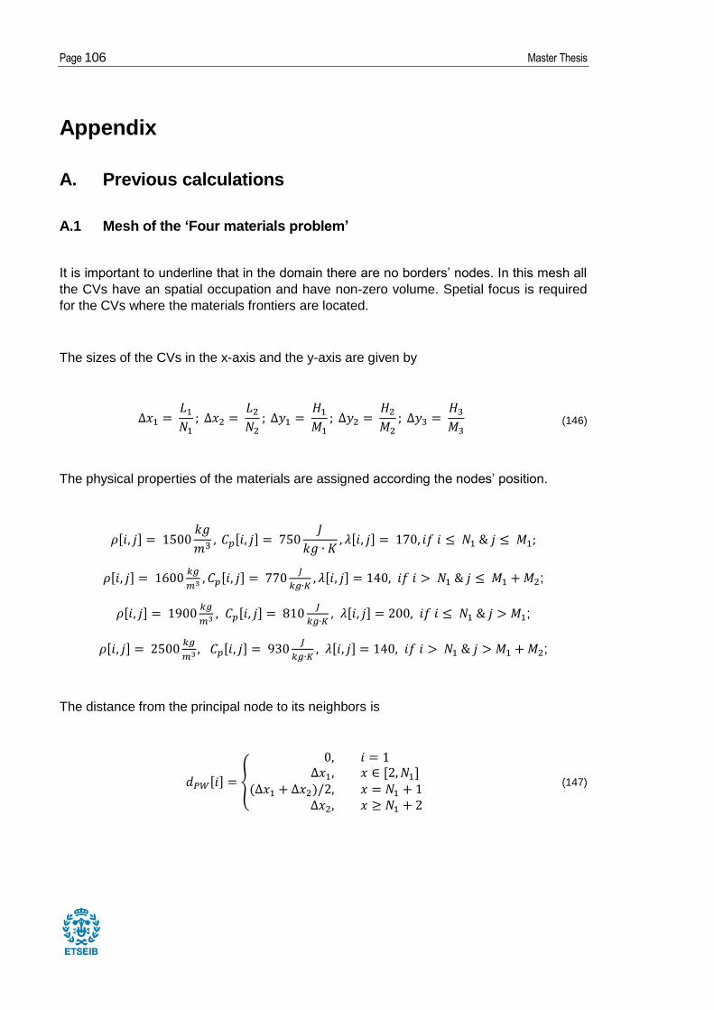
Page 106 Master Thesis
Appendix
A. Previous calculations
A.1 Mesh of the ‘Four materials problem’
It is important to underline that in the domain there are no borders’ nodes. In this mesh all
the CVs have an spatial occupation and have non-zero volume. Spetial focus is required
for the CVs where the materials frontiers are located.
The sizes of the CVs in the x-axis and the y-axis are given by
(146)
The physical properties of the materials are assigned according the nodes’ position.
;
;
;
The distance from the principal node to its neighbors is
(147)
Numerical methods in heat transfer and fluid dynamics Page 107
(148)
(149)
(150)
The distance from the principal node to the HT surfaces is
(151)
(152)
The distance from the CVs’ faces to the neighbors is
(153)
(154)
Page 108 Master Thesis
(155)
(156)
The HT surfaces and the volume of the CVs depend on their position
(157)
(158)
(159)
The nodes are classified in internal nodes and boundary nodes
Internal nodes , and .
Left side nodes ,
Top-side nodes .
The thermal conductivity of the principal and neighbors’ nodes is
Internal nodes
Left side nodes
Top-side nodes
The harmonic mean conductivity21 in the CV faces is:
21 Mandatory for internal, left-side and top-side nodes. Meanwhile, in the left-side nodes it is
not necessary to define , and in the case of the top-side nodes is for and is for
; the purpose is just to establish a limit between the walls when modeling the
mesh.
Numerical methods in heat transfer and fluid dynamics Page 109
(160)
(161)
(162)
(163)
Note that if the face under analysis is limited by CVs of equal thermal conductivity, the
harmonic mean will result in the same thermal conductivity. This is in the case the thermal
conductivity does not vary within a given material. Nevertheless, the thermal conductivity
could vary within a material if the nodes’ temperatures vary as well. In that case, it is a good
practice to calculate the thermal conductivity harmonic mean of all the faces of all the nodes.
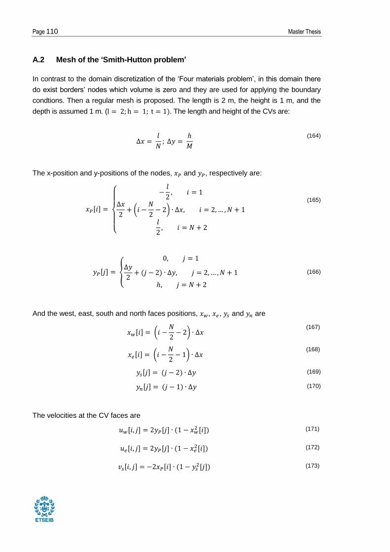
Page 110 Master Thesis
A.2 Mesh of the ‘Smith-Hutton problem’
In contrast to the domain discretization of the ‘Four materials problem’, in this domain there
do exist borders’ nodes which volume is zero and they are used for applying the boundary
condtions. Then a regular mesh is proposed. The length is 2 m, the height is 1 m, and the
depth is assumed 1 m. ( . The length and height of the CVs are:
(164)
The x-position and y-positions of the nodes, and , respectively are:
(165)
(166)
And the west, east, south and north faces positions, , , and are
(167)
(168)
(169)
(170)
The velocities at the CV faces are
(171)
(172)
(173)

Numerical methods in heat transfer and fluid dynamics Page 111
(174)
The mass flow at face ‘f’ is given by
(175)
The CVs’ surfaces and volume are constant throughout the domain and do not depend on
their position.
(176)
(177)
(178)
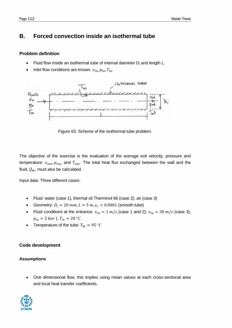
Page 112 Master Thesis
B. Forced convection inside an isothermal tube
Problem definition
Fluid flow inside an isothermal tube of internal diameter Di and length L.
Inlet flow conditions are known: .
Figure 63. Scheme of the isothermal tube problem.
The objective of the exercise is the evaluation of the average exit velocity, pressure and
temperature: and . The total heat flux exchanged between the wall and the
fluid, must also be calculated.
Input data. Three different cases:
Fluid: water (case 1), thermal oil Therminol 66 (case 2), air (case 3)
Geometry: (smooth tube)
Fluid conditions at the entrance. (case 1 and 2), (case 3),
), .
Temperature of the tube:
Code development
Assumptions
One dimensional flow, this implies using mean values at each cross-sectional area
and local heat transfer coefficients.

Numerical methods in heat transfer and fluid dynamics Page 113
Steady-state
Constant temperature of the wall.
Empirical inputs needed (local heat transfer coefficient, friction factor and
thermophysical properties) for the different fluids are evaluated from the expressions
given in the Formulae (sections C2, C7 and D0).
Heat transfer phenomena: only convection.
Domain discretization
Figure 64. Discretization of the isothermal tube.
N is the number of control volumes (CV) and N+1 is the number of nodes. The solution
approach is to calculate the fluid temperature, pressure and velocity, from node to node and
use the conservative equations for each CV. This is, formulate the conservative equations for
CV 1 and calculate the fluid properties of node 2, formulate the conservative equations for
CV 2 and calculate fluid properties of node 3, and so on until arriving to CV N and calculate
the fluid properties of node N+1.
The length of each control volume in the axial axis, , is given by:
Note that the cross-sectional surface, , is constant and it is given by:
Page 114 Master Thesis
Mass conservation equation
The unsteady term can be neglected since steady state is assumed. The transport term
represents the net mass flow that exits the control surfaces.
The mass flow is constant in all the control volumes.
The density of the fluid can be evaluated using algebraic correlations given in the Formulae
Section D. This equation is known as the state equation. The inlet density, , must be
evaluated to obtain the mass flow . The fluid density depends on the temperature and
pressure of the fluid, this is the case for the air, but it is approximated as a function only of
the temperature in the case of water and Therminol 66.
From Equation 4 and considering the control surface constant across the tube, the mass
conservation equation turns into:
Numerical methods in heat transfer and fluid dynamics Page 115
Momentum conservation equation
The unsteady term can be neglected since steady state is assumed. The transport term
represents the net linear momentum that exits the control surfaces. The third term represents
the forces acting over the control surfaces and it is positive in the coordinate positive
direction, this implies the fluid forces crossing the inlet and outlet of the control volume and
the viscous forces fluid-tube ( ). The viscous tensions are neglected. The fourth term
is equal to 0, since the gravity in the axial coordinate does not exist.
It is assumed that is constant across the control surface, then it can be placed out of the
integral. is given by:
is the skin friction coefficient and depends on the cross-sectional shape, the hydraulic
diameter (in this exercise , the Reynolds number (Re) and the relative roughness ( ).
In this exercise the cross-sectional shape is a circular tube and the relative roughness is
(smooth tube). Considering this the friction factor results:
Page 116 Master Thesis
is the average density in the control volume ‘i’ and it is evaluated at the mean temperature
(and the mean pressure in the case of air) of the control volume.
Where
is the average velocity in the control volume ‘i’ and it is the arithmetic mean of and
.
Then the Equation 10 can be expressed as:
Energy conservation equation
The unsteady term can be neglected since steady state is assumed. The transport term
represents the net energy that exits the control surfaces, here, the potential energy variation
is neglected, and the kinetic energy variation can be neglected for liquids if wanted. The third
term represents the net heat flux that enters through the control surfaces. The fourth term
Numerical methods in heat transfer and fluid dynamics Page 117
represents the work developed and in this exercise is equal to 0.
The third term in this exercise is given by heat exchanged between the tube and the fluid
through the cylindrical surface. Considering the heat transfer coefficient constant across a
CV, and taking the mean temperature of the fluid in the CV, we obtain
If the fluid is air, is treated as a semi-perfect gas, then the enthalpy differential is
If the fluid is a liquid (in the case of water and Therminol 66), the enthalpy differential is:
The component
can be neglected as it is some orders of magnitude smaller than
. Then it is obtained
In forced convection inside ducts, to obtain the heat transfer coefficient, , the
thermophysical properties of the fluid (dynamic viscosity, thermal conductivity and specific
heat) must be obtained first, and these are evaluated at the mean fluid bulk temperature, .
, , , .
refers to the fluid viscosity if it were at the temperature of the tube.
Next, the non-dimensional numbers are obtained: Re, Pr, Gz and Nu.
Page 118 Master Thesis
For laminar flow ( < 2000):
For turbulent flow ( > 2000):
Finally, the heat transfer coefficient of the CV ‘i', , is given by
Finally, this heat transfer coefficient is used in the energy conservation equation.
Numerical methods in heat transfer and fluid dynamics Page 119
Algorithm
1. Input data:
Physical data: .
Numerical data: .
2. Previous calculations: .
3. Initial map: For node i = 1. where . The fluid properties at
the inlet are already known.
4. Evaluation of node ‘i+1’.
Guess the fluid properties at node ‘i+1’: , where
Evaluate the thermophysical properties of the fluid: at the mean
bulk temperature and pressure, and .
Calculate the non-dimensional numbers (Re, Pr, Gz, Nu), the heat transfer
coefficient ( ), and the friction factor .
Calculate the fluid properties from the conservative equations
From the linear momentum conservation equation, calculate .
From the energy conservation equation, calculate .
From the state equation, calculate .
From the mass conservation equation, calculate .
5. Convergence criteria:
Is , where
If no: . (Refresh the guessed fluid properties to the last calculated
values); and go to 4.2.
If yes: Go to 6.
6. Is i = N+1? (Evaluation of the last node).
If NO: Update the node: i i+1. Go to 4.1
If YES: Go to 7.
7. Final calculations: and
.
8. Print results: vs. x, where and x is the axial coordinate.
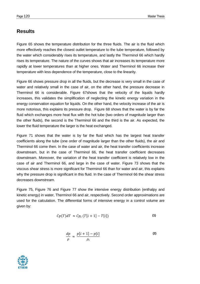
Page 120 Master Thesis
Results
Figure 65 shows the temperature distribution for the three fluids. The air is the fluid which
more effectively reaches the closest outlet temperature to the tube temperature, followed by
the water which considerably rises its temperature, and lastly the Therminol 66 which hardly
rises its temperature. The nature of the curves shows that air increases its temperature more
rapidly at lower temperatures than at higher ones. Water and Therminol 66 increase their
temperature with less dependence of the temperature, close to the linearity.
Figure 66 shows pressure drop in all the fluids, but the decrease is very small in the case of
water and relatively small in the case of air, on the other hand, the pressure decrease in
Therminol 66 is considerable. Figure 67shows that the velocity of the liquids hardly
increases, this validates the simplification of neglecting the kinetic energy variation in the
energy conservation equation for liquids. On the other hand, the velocity increase of the air is
more notorious, this explains its pressure drop. Figure 68 shows that the water is by far the
fluid which exchanges more heat flux with the hot tube (two orders of magnitude larger than
the other fluids), the second is the Therminol 66 and the third is the air. As expected, the
lower the fluid temperature the larger is the heat exchanged.
Figure 71 shows that the water is by far the fluid which has the largest heat transfer
coefficients along the tube (one order of magnitude larger than the other fluids), the air and
Therminol 66 come then. In the case of water and air, the heat transfer coefficients increase
downstream, but in the case of Therminol 66, the heat transfer coefficient decreases
downstream. Moreover, the variation of the heat transfer coefficient is relatively low in the
case of air and Therminol 66, and large in the case of water. Figure 73 shows that the
viscous shear stress is more significant for Therminol 66 than for water and air, this explains
why the pressure drop is significant in this fluid. In the case of Therminol 66 the shear stress
decreases downstream.
Figure 75, Figure 76 and Figure 77 show the intensive energy distribution (enthalpy and
kinetic energy) in water, Therminol 66 and air, respectively. Second order approximations are
used for the calculation. The differential forms of intensive energy in a control volume are
given by:
(1)
(2)
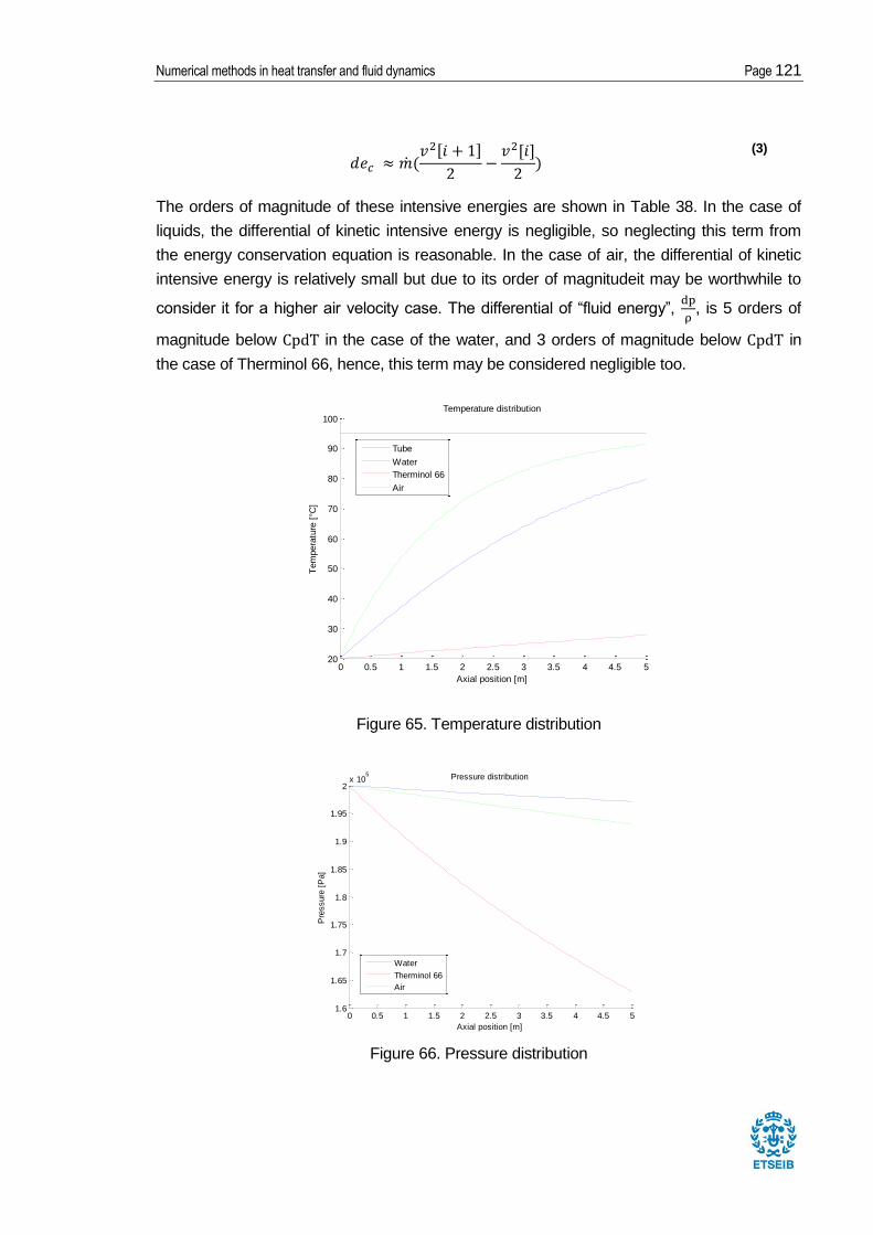
Numerical methods in heat transfer and fluid dynamics Page 121
(3)
The orders of magnitude of these intensive energies are shown in Table 38. In the case of
liquids, the differential of kinetic intensive energy is negligible, so neglecting this term from
the energy conservation equation is reasonable. In the case of air, the differential of kinetic
intensive energy is relatively small but due to its order of magnitudeit may be worthwhile to
consider it for a higher air velocity case. The differential of “fluid energy”,
, is 5 orders of
magnitude below in the case of the water, and 3 orders of magnitude below in
the case of Therminol 66, hence, this term may be considered negligible too.
Figure 65. Temperature distribution
Figure 66. Pressure distribution
0 0.5 1 1.5 2 2.5 3 3.5 4 4.5 520
30
40
50
60
70
80
90
100
Axial position [m]
Tem
pera
ture
[°C
]
Temperature distribution
Tube
Water
Therminol 66
Air
0 0.5 1 1.5 2 2.5 3 3.5 4 4.5 51.6
1.65
1.7
1.75
1.8
1.85
1.9
1.95
2x 10
5
Axial position [m]
Pre
ssure
[P
a]
Pressure distribution
Water
Therminol 66
Air
Page 122 Master Thesis
Figure 67. Velocity distribution
Figure 68. Velocity distribution
Figure 69. Heat flux distribution
0 0.5 1 1.5 2 2.5 3 3.5 4 4.5 50
5
10
15
20
25
30
35
40
Axial position [m]
Velc
oity [
m/s
]
Velocity distribution
Water
Therminol 66
Air
0 0.5 1 1.5 2 2.5 3 3.5 4 4.5 5
0.98
0.99
1
1.01
1.02
1.03
1.04
Axial position [m]
Velc
oity [
m/s
]
Velocity distribution
Water
Therminol 66
Air
0 0.5 1 1.5 2 2.5 3 3.5 4 4.5 50
200
400
600
800
1000
1200
Axial position [m]
Heat
flux [
W]
Heat flux distribution
Water
Therminol 66
Air
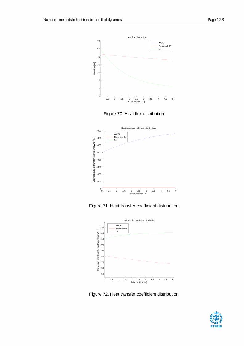
Numerical methods in heat transfer and fluid dynamics Page 123
Figure 70. Heat flux distribution
Figure 71. Heat transfer coefficient distribution
Figure 72. Heat transfer coefficient distribution
0.5 1 1.5 2 2.5 3 3.5 4 4.5 5-10
0
10
20
30
40
50
60
Axial position [m]
Heat
flux [
W]
Heat flux distribution
Water
Therminol 66
Air
0 0.5 1 1.5 2 2.5 3 3.5 4 4.5 50
1000
2000
3000
4000
5000
6000
7000
8000
Axial position [m]
Convection h
eat
transfe
r coeff
icie
nt
[W/m
2 K
]
Heat transfer coefficient distribution
Water
Therminol 66
Air
0 0.5 1 1.5 2 2.5 3 3.5 4 4.5 5
150
160
170
180
190
200
210
220
230
Axial position [m]
Convection h
eat
transfe
r coeff
icie
nt
[W/m
2 K
]
Heat transfer coefficient distribution
Water
Therminol 66
Air
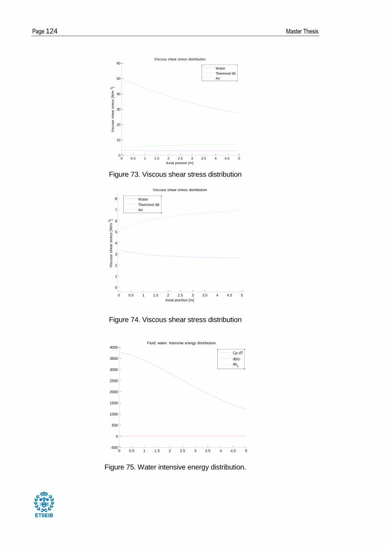
Page 124 Master Thesis
Figure 73. Viscous shear stress distribution
Figure 74. Viscous shear stress distribution
Figure 75. Water intensive energy distribution.
0 0.5 1 1.5 2 2.5 3 3.5 4 4.5 50
10
20
30
40
50
60
Axial position [m]
Vis
cous s
hear
str
ess [
N/m
2]
Viscous shear stress distribution
Water
Therminol 66
Air
0 0.5 1 1.5 2 2.5 3 3.5 4 4.5 5
0
1
2
3
4
5
6
7
8
Axial position [m]
Vis
cous s
hear
str
ess [
N/m
2]
Viscous shear stress distribution
Water
Therminol 66
Air
0 0.5 1 1.5 2 2.5 3 3.5 4 4.5 5-500
0
500
1000
1500
2000
2500
3000
3500
4000Fluid: water. Intensive energy distribution.
Cp dT
dp/
dec
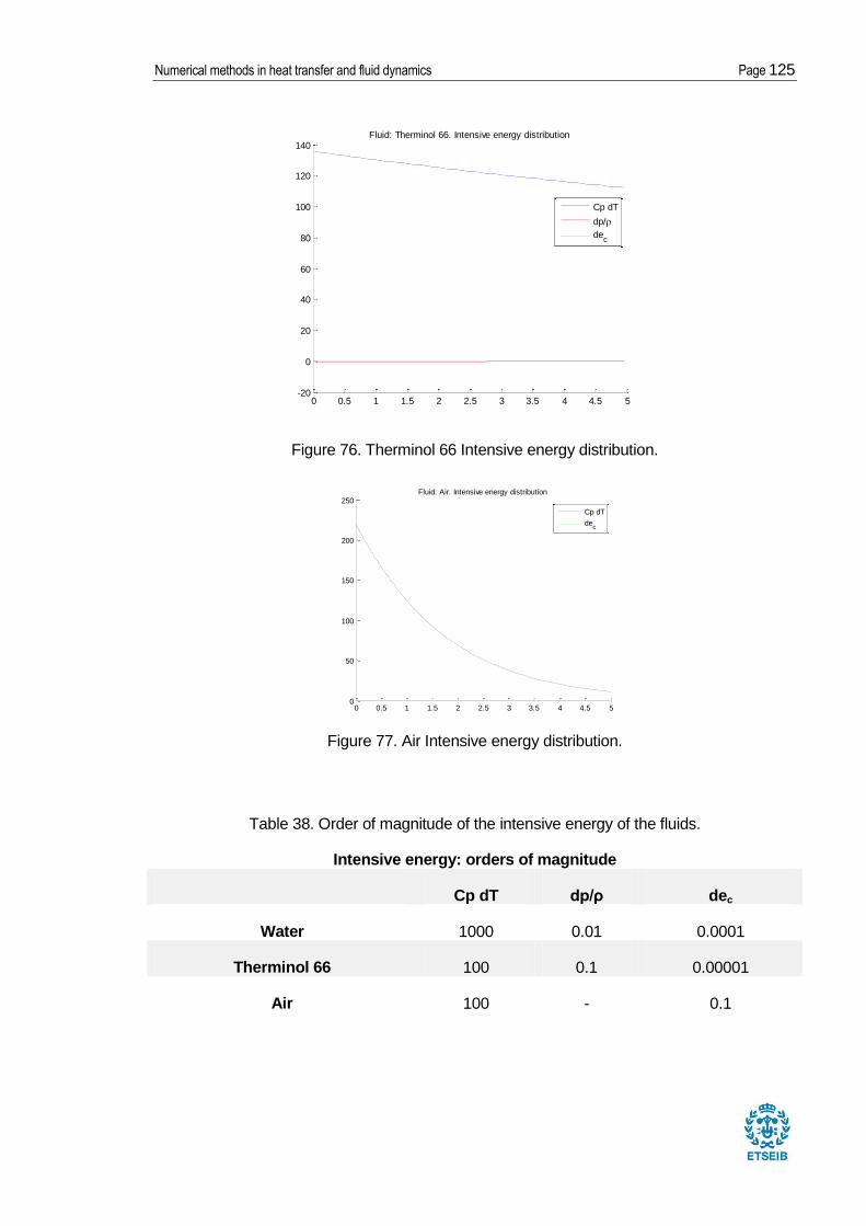
Numerical methods in heat transfer and fluid dynamics Page 125
Figure 76. Therminol 66 Intensive energy distribution.
Figure 77. Air Intensive energy distribution.
Table 38. Order of magnitude of the intensive energy of the fluids.
Intensive energy: orders of magnitude
Cp dT dp/ρ dec
Water 1000 0.01 0.0001
Therminol 66 100 0.1 0.00001
Air 100 - 0.1
0 0.5 1 1.5 2 2.5 3 3.5 4 4.5 5-20
0
20
40
60
80
100
120
140Fluid: Therminol 66. Intensive energy distribution
Cp dT
dp/
dec
0 0.5 1 1.5 2 2.5 3 3.5 4 4.5 50
50
100
150
200
250Fluid: Air. Intensive energy distribution
Cp dT
dec

Page 126 Master Thesis
Validation
Table 39 shows the fluid properties obtained at the outlet of the tube. Table 40 shows the
relative error of the results regarding the results obtained using an analytical solution. In all
the cases, the relative error is small enough. The numerical data used to solve the problem
are: and .
Table 39. Fluid properties at the outlet of the tube.
Fluid properties at the outlet
Fluid T [°C] p [Pa] v [m/s]
Water 79.52 197141 1.026
Therminol 66 27.75 163038 1.005
Air 91.31 193021 38.647
Table 40. Relative error regarding the analytical solution results.
Relative error
Fluid T [°C] p [Pa] v [m/s]
Water 0.99% 0.00% 0.05%
Therminol 66 0.04% 0.20% 0.00%
Air 0.13% 0.25% 0.22%
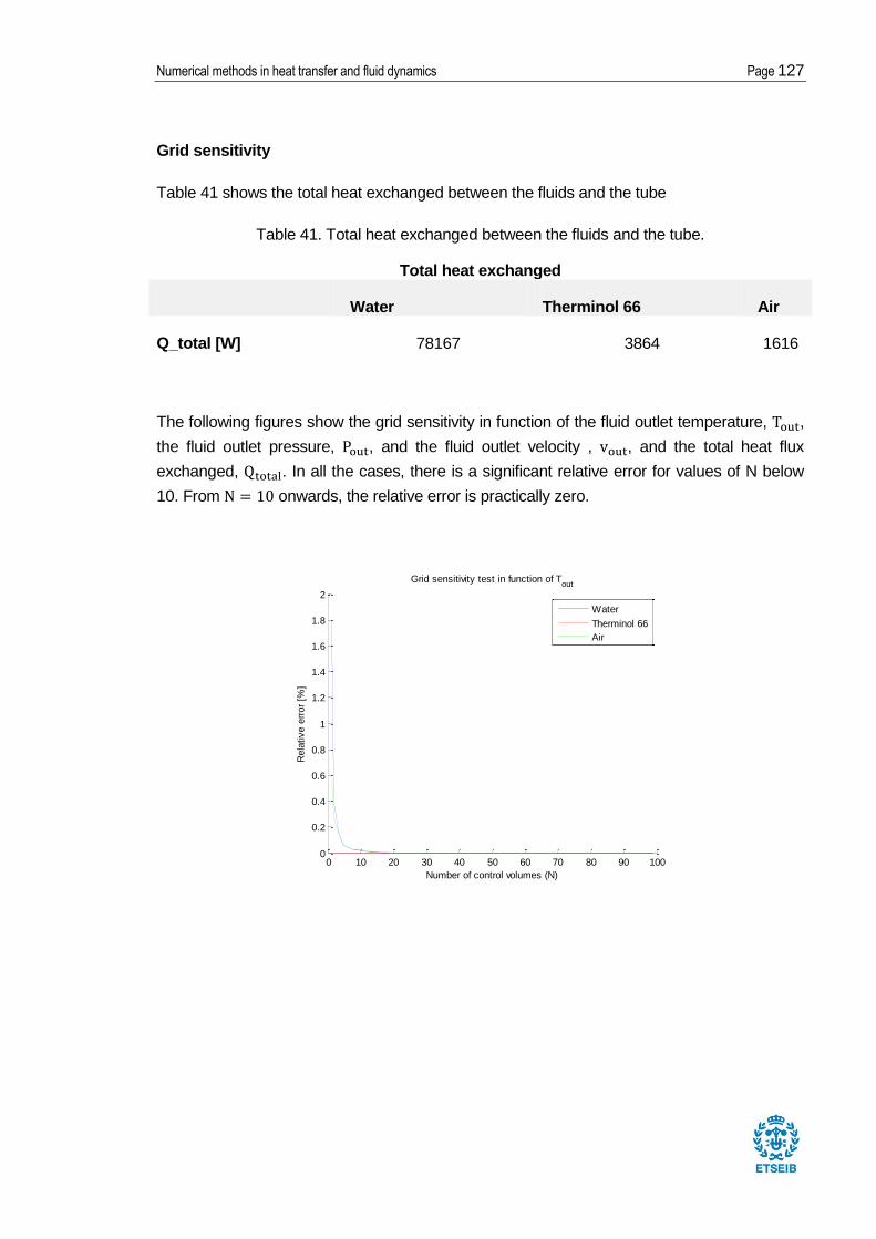
Numerical methods in heat transfer and fluid dynamics Page 127
Grid sensitivity
Table 41 shows the total heat exchanged between the fluids and the tube
Table 41. Total heat exchanged between the fluids and the tube.
Total heat exchanged
Water Therminol 66 Air
Q_total [W] 78167 3864 1616
The following figures show the grid sensitivity in function of the fluid outlet temperature, ,
the fluid outlet pressure, , and the fluid outlet velocity , , and the total heat flux
exchanged, . In all the cases, there is a significant relative error for values of N below
10. From onwards, the relative error is practically zero.
0 10 20 30 40 50 60 70 80 90 1000
0.2
0.4
0.6
0.8
1
1.2
1.4
1.6
1.8
2
Number of control volumes (N)
Rela
tive e
rror
[%]
Grid sensitivity test in function of Tout
Water
Therminol 66
Air
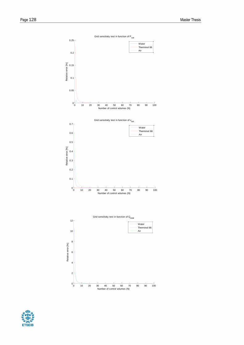
Page 128 Master Thesis
0 10 20 30 40 50 60 70 80 90 1000
0.05
0.1
0.15
0.2
0.25
Number of control volumes (N)
Rela
tive e
rror
[%]
Grid sensitivity test in function of Pout
Water
Therminol 66
Air
0 10 20 30 40 50 60 70 80 90 1000
0.1
0.2
0.3
0.4
0.5
0.6
0.7
Number of control volumes (N)
Rela
tive e
rror
[%]
Grid sensitivity test in function of vout
Water
Therminol 66
Air
0 10 20 30 40 50 60 70 80 90 1000
2
4
6
8
10
12
Number of control volumes (N)
Rela
tive e
rror
[%]
Grid sensitivity test in function of Qtotal
Water
Therminol 66
Air
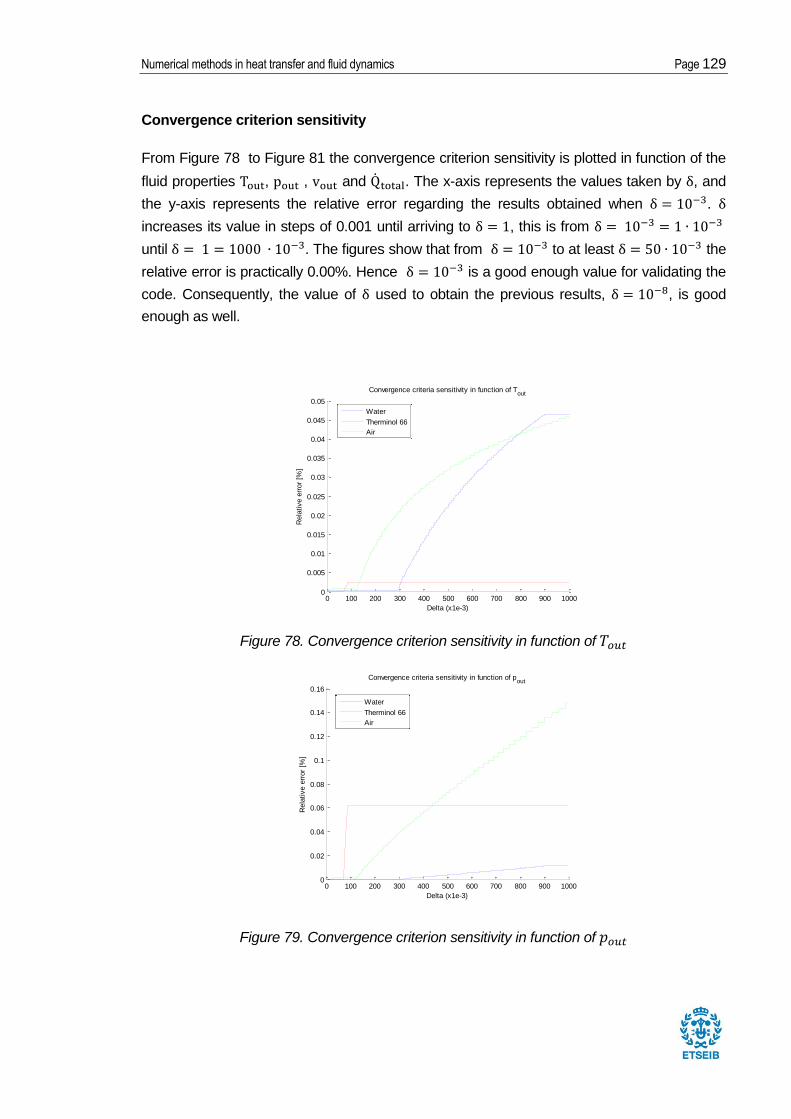
Numerical methods in heat transfer and fluid dynamics Page 129
Convergence criterion sensitivity
From Figure 78 to Figure 81 the convergence criterion sensitivity is plotted in function of the
fluid properties , , and . The x-axis represents the values taken by , and
the y-axis represents the relative error regarding the results obtained when .
increases its value in steps of 0.001 until arriving to , this is from
until . The figures show that from to at least the
relative error is practically 0.00%. Hence is a good enough value for validating the
code. Consequently, the value of used to obtain the previous results, , is good
enough as well.
Figure 78. Convergence criterion sensitivity in function of
Figure 79. Convergence criterion sensitivity in function of
0 100 200 300 400 500 600 700 800 900 10000
0.005
0.01
0.015
0.02
0.025
0.03
0.035
0.04
0.045
0.05
Delta (x1e-3)
Rela
tive e
rror
[%]
Convergence criteria sensitivity in function of Tout
Water
Therminol 66
Air
0 100 200 300 400 500 600 700 800 900 10000
0.02
0.04
0.06
0.08
0.1
0.12
0.14
0.16
Delta (x1e-3)
Rela
tive e
rror
[%]
Convergence criteria sensitivity in function of pout
Water
Therminol 66
Air

Page 130 Master Thesis
Figure 80. Convergence criterion sensitivity in function of
Figure 81. Convergence criterion sensitivity in function of
Discussion
If the objective were reaching the temperature of the tube:
A double-length tube is needed in the case of air for reaching the
temperature of the tube in 99.8%
A double-length tube is needed in the case of water for reaching the
0 100 200 300 400 500 600 700 800 900 10000
0.02
0.04
0.06
0.08
0.1
0.12
Delta (x1e-3)
Rela
tive e
rror
[%]
Convergence criteria sensitivity in function of vout
Water
Therminol 66
Air
0 100 200 300 400 500 600 700 800 900 10000
0.05
0.1
0.15
0.2
0.25
0.3
0.35
Delta (x1e-3)
Rela
tive e
rror
[%]
Convergence criteria sensitivity in function of Qtotal
Water
Therminol 66
Air
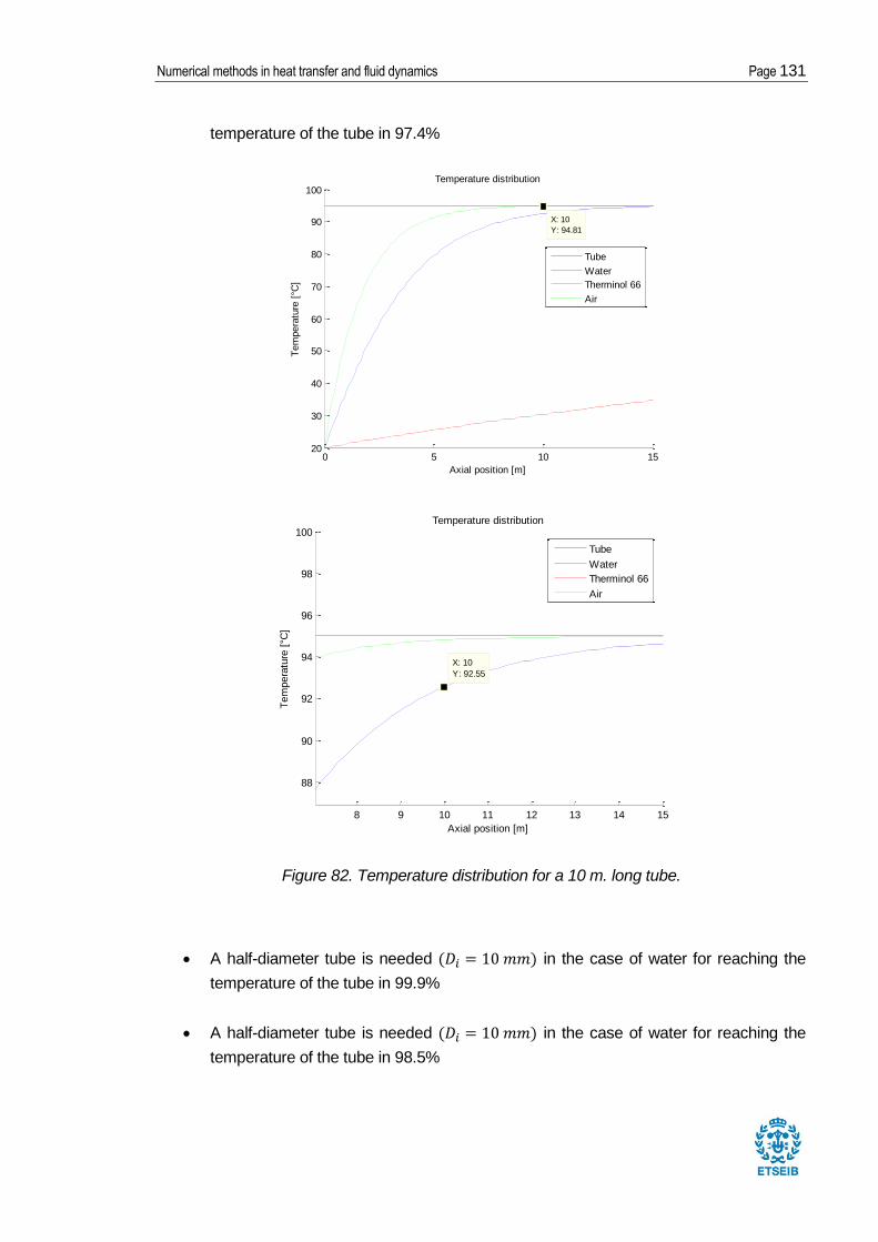
Numerical methods in heat transfer and fluid dynamics Page 131
temperature of the tube in 97.4%
Figure 82. Temperature distribution for a 10 m. long tube.
A half-diameter tube is needed in the case of water for reaching the
temperature of the tube in 99.9%
A half-diameter tube is needed in the case of water for reaching the
temperature of the tube in 98.5%
0 5 10 1520
30
40
50
60
70
80
90
100
X: 10
Y: 94.81
Axial position [m]
Tem
pera
ture
[°C
]
Temperature distribution
Tube
Water
Therminol 66
Air
8 9 10 11 12 13 14 15
88
90
92
94
96
98
100
X: 10
Y: 92.55
Axial position [m]
Tem
pera
ture
[°C
]
Temperature distribution
Tube
Water
Therminol 66
Air
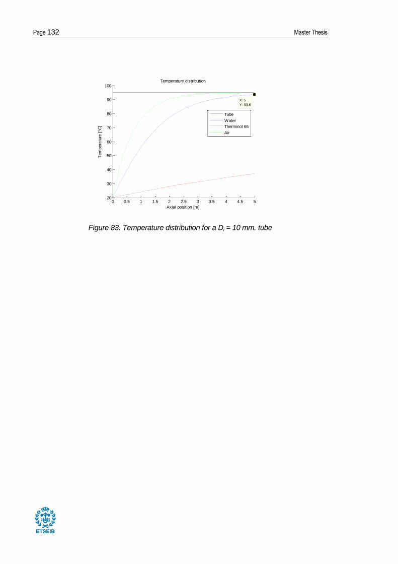
Page 132 Master Thesis
Figure 83. Temperature distribution for a Di = 10 mm. tube
0 0.5 1 1.5 2 2.5 3 3.5 4 4.5 520
30
40
50
60
70
80
90
100
X: 5
Y: 93.6
Axial position [m]
Tem
pera
ture
[°C
]
Temperature distribution
Tube
Water
Therminol 66
Air