FLM

Technische Universität München

Lehrstuhl für Fluidmechanik

o. Prof. Dr.-Ing. habil. Dr. h.c. Rudolf Schilling

JASS 2009-Joint Advanced Student School, St. Petersburg, 29.3.-7.4.2009 Numerical Simulation in Turbomachinery

Numerical Simulation of the Active Flow Control in Turbomachinery

Wunderer R. Technische Universität München, Lehrstuhl für Fluidmechanik, D-85747 Garching, Germany

Contents 1. INTRODUCTION 2. NUMERICAL DETAILS 3. RESULTS 4. SUMMARY

ABSTRACT ii

ABSTRACT

Hydro Turbines are being operated on very high levels of efficiency, characterised by peak efficiencies beyond 95%. Thus, the margin for further increasing the efficiencies in the best point of operation and in the vicinity of it is very small. However, considering operating points away from the optimum, in extreme part or over load operation, the efficiency drop may be very high. This phenomenon is combined with a strong increase of the pressure pulsations, decreasing the life endurance limit of turbines.

To reduce the time-dependent pressure loading of Francis turbine runners several possibilities of active flow control have been studied. The most promising solution to reduce the time-dependent pressure loading of turbine runners is the excitation of the flow by pitching the guide vanes with variable frequencies and amplitudes. To investigate this fluid flow problem in detail an LES code has been developed and applied to solve it.

The paper shows simulation results for a 2D tandem cascade as well as for a Francis Turbine runner of specific speed nq = 85 min-1. The simulations were carried out with different parameter combinations regarding the frequency and the amplitude of the pitching guide vanes. The results show that the losses can be reduced considerably, concerning the tandem cascade and the hydraulic efficiency can be increased, concerning the radial runner. Furthermore the amplitude of the pressure pulsations can be diminished as well as their characteristic frequencies can be shifted towards lower or higher values. Thus, a resonance effect in the turbine may be avoided by modifying the pitching frequency.

CONTENTS iii

CONTENTS

ABSTRACT ............................................................................................................................ii CONTENTS ...........................................................................................................................iii NOMENCLATURE ............................................................................................................... iv 1. INTRODUCTION ............................................................................................................... 1 2. NUMERICAL DETAILS.................................................................................................... 1

2.1. CFD code...................................................................................................................... 1 2.2. DES models .................................................................................................................. 2 2.3. Boundary layer shielding.............................................................................................. 2 2.4. Hybrid differencing ...................................................................................................... 3

3. RESULTS............................................................................................................................ 5

3.1. Translational tandem cascade....................................................................................... 5 3.1.4. Fixed guide vanes .................................................................................................. 6 3.1.5. Pitching guide vanes.............................................................................................. 6

3.2. Radial blade row......................................................................................................... 10 3.2.1. Steady flow onto the runner................................................................................. 11 3.2.2. Time varying flow onto the runner...................................................................... 12

4. SUMMARY....................................................................................................................... 17 REFERENCES ...................................................................................................................... 17

NOMENCLATURE iv

NOMENCLATURE

Letters CDES [-] DES model constant N [-] number of blades rms root mean square F [N] force M [Nm] torque Q [m3/s] flow rate c [m/s] velocity vector d [m] distance to the nearest wall f [1/s] frequency k [m2/s2], turbulent kinetic energy, [-] reduced frequency l [m] blade length nq [1/min] specific speed pt [N/m2] total pressure r [m] radius t [s] time x [m] coordinate

Δ [m] local grid spacing β* [-] k-ω model constant κ [-] von Karman constant ν [m2/s] kinematic viscosity νt [m2/s] turbulent kinematic viscosity ρ [kg/m3] density ω [1/s], specific dissipation rate, [rad/s] angular velocity

Subscripts and Superscripts

c, b crown, band n normal direction f regarding the force i component of a vector p regarding the pressure r radial component of a vector m meridional component of a vector, regarding the torque n regarding the normal force opt regarding the optimum point of operation u circumferential component of a vector x, y, z cartesian directions 0 value at the inlet 1,2 blade inlet, outlet

1. INTRODUCTION 1

1. INTRODUCTION

Francis turbines are characterized by peak efficiencies beyond 95%. This is only valid in the best point of operation. However in part and over load the efficiency drops significantly. Furthermore pressure pulsations can be observed in this operation points. In large Francis turbines the pulsations can cause very large resulting forces on the runner blades. These forces can impair the life endurance of the runner blades and therefore damage them in the long run. Damage may also occur, if the fluctuations stimulate the turbine with its eigenfrequency. To avoid damages and expensive repairs, the turbines are switched off in the case of extremely water levels.

For both effects, the drop of efficiency and the pressure pulsations, the reason is a highly transitional flow in the rotor. At the leading edges of the rotor blades a massive separation can occur, which is the main cause for the transitional flow character.

Active flow control can reduce this separation and therefore increase the efficiency and modify the pressure pulsations, regarding amplitude reduction and frequency shifting. By pitching the guide vanes periodically, a time varying flow onto the runner blades is created which affects the separation in the desired way.

For the investigation of these phenomenons numerical simulations were done. Therefore a hybrid turbulence modelling, namely Detached Eddy Simulation (DES) was applied. Some modifications regarding the underlying DES-model and the handling of the discretization of the advection terms were done. Thus it was managed to apply DES for the flow in turbo-machines.

2. NUMERICAL DETAILS

2.1. CFD code An efficient 3D transient Navier-Stokes code, based on a Finite Volume formulation, was developed. The linearized system of momentum- and continuity equations is solved by a modified version of the PISO pressure correction scheme, which original formulation was described by ISSA [1]. With this code several simulations were done, to investigate the physical details of the transient flow and the effects of the active flow control in a turbine under part load conditions.

The need to simulate pitching airfoils required to handle mesh deformation. Therefore the space conservation law, s. FERZIGER AND PERIC [2], which modifies the fluxes in the Navier-Stokes equations in the case of mesh deformation, was implemented. For an efficient and accurate mesh deformation, an algorithm has been developed. It is based on an algebraic formulation and works without solving any extra partial differential equations. The algorithm was optimized for the problem of pitching airfoils and the validation regarding mesh quality showed, that it was superior to Finite Volume and Finite Element approaches for this kind of problem. The algorithm is described in [3].

2. NUMERICAL DETAILS 2

2.2. DES models Preliminary simulations showed that the physical effects, that should be studied, could not be resolved with a Reynolds Averaged Navier-Stokes (RANS) simulation, s. [4]. The desired accuracy can be achieved with a Large Eddy Simulation (LES). However classical LES needs to resolve the wall near domain very accurately. The resolution is dependent on the Reynolds number of the flow (Re). PIOMELLI AND BALARAS [5] showed, that the number of cells, required to resolve just the inner part of the boundary layer is ~Re1.8. The time step has to be adapted accordingly. In technical flows of the kind studied here, Reynolds numbers of ~106 are examined. The required computing power is far-off today´s available resources. Therefore it is necessary to model the boundary layer.

Most promising for that task is the DES, which uses a hybrid turbulence model acting as a RANS model in the boundary domain and an LES subgrid scale (SGS) model outside it, s. [6, 7]. The switching between the two modes is done by the model itself. Some DES models where validated e.g. in [4]. For the following calculations the SST-DES model was chosen. The equations for that model are shown e.g. in MENTER AND KUNTZ [8].

2.3. Boundary layer shielding The major drawback of the original DES formulation is the grid dependency of the mechanism for switching between the LES and the RANS mode of the model. To achieve good results the grid has to be adapted exactly to the given flow. To avoid that problem several shielding mechanisms for the boundary layer have been developed, s. e.g. MENTER AND KUNTZ [8] or SPALART ET AL. [9]. Independently of the grid quality these mechanisms should prevent the model from switching to the LES mode in domains where the RANS mode should be active, especially in the wall near domains. In WUNDERER AND SCHILLING [10] an adaptation of the shielding for the SST-DES model was done, which allows using DES in turbomachinery. More details on this can be found in [10]. The formulation of the DES-limiter FDES for the model is:

( ) ⎟

⎠

⎞⎜⎝

⎛ −−−=

0111

1

,k

CmaxFF

*DESd

DES ωβΔ (1)

( )

3

22

8⎟⎟

⎠

⎞

⎜⎜

⎝

⎛ +=

dcctanhF

j,ij,i

td

κνν

(2)

The advantage of this new formulation is its applicability for internal turbulent flows, as in turbo-machines. It ensures, that the RANS mode of the model is activated just inside the boundary layer, whereas the LES mode is activated outside it. The common method of shielding the SST-model activates the RANS mode in a much too large flow domain. A comparison of both methods can be seen in Fig. 1 and 2.

2. NUMERICAL DETAILS 3

Figure 1: Model mode for the flow in a blade row, with the new shielding, regarding equ. 1

Figure 2: Model mode for the flow in a blade row, with the shielding, proposed by MENTER AND KUNTZ [8]

2.4. Hybrid differencing For LES or LES-like simulations as DES or SAS, s. MENTER AND EGOROV [11], the discretization scheme should be of central-differencing type (CDS). This is due to the fact that central-differencing schemes are less dissipative than upwind schemes (UDS) and thus full advantage of the grid provided can be taken. However CDS is less stable than UDS. Among other things this can be caused by nonuniform grids or too high cell Reynolds numbers.

To combine the advantages of both schemes, TRAVIN ET AL. [12] developed a hybrid differencing scheme that blends the fluxes calculated both by a CDS and a UDS. The blending function switches between a UDS near the walls and in the domains where the turbulence intensity as well as the transient character of the flow is low and a CDS elsewhere. The blending function by TRAVIN ET AL. [12] was applied for the simulations of the flow in the tandem cascade, but was not appropriate for the simulations of the flow in the radial turbine runner. Therefore an alternative formulation of the blending function was used, which is described in WUNDERER AND SCHILLING [13]. The flow in the runner is visualized by the vectors of the relative velocity on a plane section, in Fig. 3. The blending works in a way, that regions with a high transient flow character are preferred for the CDS. Additionally the influence of the grid is taken into account, what means, that mesh regions of poor quality are discretized by UDS. In the following equations τmin and τmax are representative convection times of a cell. This can e.g. be the minimum and maximum time of the flow needed to pass a cell. The blending is described bellow. In Fig. 4 and 5 it can be seen that the blending works as desired. The flow within the runner is dominated by CDS, whereas outside the runner there is added some amount of UDS.

2. NUMERICAL DETAILS 4

The new blending function is defined as follows:

( ) ( ) BBC

maxHAtanh σσσσ +−⋅⋅= 11 (3)

( )( )( )

US,maxCB

,Btanhmaxgc

kL

,.gL

CmaxCA

maxH

turb

turb

maxDESH

ΔΩ

ω

Δ

μ

⋅⋅=

=

=

⎟⎟⎠

⎞⎜⎜⎝

⎛−⋅=

−

3

104

2

10

050

( ) ( )( )

⎟⎟⎠

⎞⎜⎜⎝

⎛+⎟

⎟⎠

⎞⎜⎜⎝

⎛⎟⎟⎠

⎞⎜⎜⎝

⎛+

⋅⋅=

−

⎟⎟⎠

⎞⎜⎜⎝

⎛−⎟⎟

⎠

⎞⎜⎜⎝

⎛

=

⋅−⋅−−=

−

−

111022

1

10

1

10

10

5151

,minsin

CC

,CC,minmax

max

minF

CU

CUmin

max

G

.

FGG.

GGB

ττπσ

ΔΔ

σ

σσσσσσ

1229131 321 ====== UCHHHmax C,C,C,C,C,σ

Figure 3: Vectors of the relative velocity, plotted on a plane section through a radial turbine

3. RESULTS 5

Figure 4: Blending factor, calculated

by equations 3

Figure 5: Blending factor by TRAVIN ET AL. [12]

3. RESULTS

3.1. Translational tandem cascade For studying the basic effects an abstract model of a radial turbine was chosen. It consists of two blade rows, the first corresponding to the guide vanes and the second corresponding to the runner. It is equivalent to a radial turbine with a very large diameter. As the two bladings are fixed, the flow corresponds to the relative flow in a radial turbine. The front blades are turned about -10° and the back blades about 37°. The model is shown in Fig. 6. The mesh consists of ~1·106 cells. A mesh study showed that this resolution was adequate for the simulations, s. [4]. The flow analysis has been done on three sections: Section 0 was placed upstream the first blade row, section 1 between the two rows and section 2 downstream the second row.

outlet

periodic

wall

inlet

Figure 6: Geometry of the tandem cascade

3. RESULTS 6

3.1.4. Fixed guide vanes The unsteady character of the flow is shown in Fig. 11, where the streamlines are plotted on a plane section. A sequence of the separation process for the case with fixed front blades can be seen there.

The frequency analysis of the blade normal force shows two characteristic peaks, s. Fig. 7. The first one at k = 3.125, which is the frequency of the separation, the second one at k = 6.25, which is the second harmonic. The reduced frequency k calculates as:

0u

lfk π= (4)

FFT (kVL = 0)

1.E-08

1.E-07

1.E-06

1.E-05

1.E-04

1.E-03

1.E-02

1.E-01

1.E+00

0.1 1 10 100k[-]

|F (c

n)|

Figure 7: Frequency spectrum of the normal force coefficient cn; case with fixed guide

vanes

The separation is not comparable with the separation at a single airfoil, as it is described e.g. in [14-16]. This is due to the fact, that there is the effect of additional blades on the flow. First the blades bound the size of the separation to a maximum value. Secondly the separation affects the flow in a positive way, as it transports fluid downwards by its rotation. This amplifies the direction change of the flow and leads to a nearly blade congruent flow at the trailing edge in this case, s. Fig. 11.

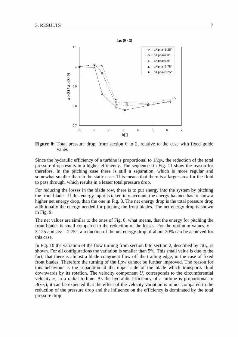
3.1.5. Pitching guide vanes To study the dynamic behaviour, the front blades where pitched with various frequencies and amplitudes. In Fig. 8 the effect on the total pressure drop from section 0 to section 2 is shown. A positive effect on the pressure drop can be seen for various frequencies and amplitudes. The total pressure drop is reduced mostly at k = 3.125. This corresponds to the frequency of the vortex-separation at the leading edges of the blades. The total pressure drop is reduced about 22%.

3. RESULTS 7

Δpt (0 - 2)

0.7

0.8

0.9

1

1.1

0 1 2 3 4 5 6 7k[-]

Δp t

(k) /

Δp t

(k=0

)

dAlpha=1.25°

dAlpha=2.0°

dAlpha=3.0°

dAlpha=3.75°

dAlpha=3.25°

Figure 8: Total pressure drop, from section 0 to 2, relative to the case with fixed guide

vanes

Since the hydraulic efficiency of a turbine is proportional to 1/Δpt, the reduction of the total pressure drop results in a higher efficiency. The sequences in Fig. 11 show the reason for therefore. In the pitching case there is still a separation, which is more regular and somewhat smaller than in the static case. This means that there is a larger area for the fluid to pass through, which results in a lesser total pressure drop.

For reducing the losses in the blade row, there is to put energy into the system by pitching the front blades. If this energy input is taken into account, the energy balance has to show a higher net energy drop, than the one in Fig. 8. The net energy drop is the total pressure drop additionally the energy needed for pitching the front blades. The net energy drop is shown in Fig. 9.

The net values are similar to the ones of Fig. 8, what means, that the energy for pitching the front blades is small compared to the reduction of the losses. For the optimum values, k = 3.125 and Δα = 2.75°, a reduction of the net energy drop of about 20% can be achieved for this case.

In Fig. 10 the variation of the flow turning from section 0 to section 2, described by ΔUy, is shown. For all configurations the variation is smaller than 5%. This small value is due to the fact, that there is almost a blade congruent flow off the trailing edge, in the case of fixed front blades. Therefore the turning of the flow cannot be further improved. The reason for this behaviour is the separation at the upper side of the blade which transports fluid downwards by its rotation. The velocity component Uy corresponds to the circumferential velocity cu in a radial turbine. As the hydraulic efficiency of a turbine is proportional to Δ(rcu), it can be expected that the effect of the velocity variation is minor compared to the reduction of the pressure drop and the influence on the efficiency is dominated by the total pressure drop.

3. RESULTS 8

Δpt_net (0 - 2)

0.7

0.8

0.9

1

1.1

0 1 2 3 4 5 6 7k[-]

(Δp t

(k) +

pPi

tchi

ng) /

Δp t

(k=0

)

dAlpha=1.25°

dAlpha=2.0°dAlpha=3.0°

dAlpha=3.75°dAlpha=3.25°

Figure 9: Net drop of total pressure, from section 0 to 2, relative to the case with fixed

guide vanes

0.9

0.95

1

1.05

1.1

0 1 2 3 4 5 6 7k[-]

ΔU

y(k)

/ Δ

Uy(

k=0)

dAlpha=1.25°

dAlpha=2.0°

dAlpha=3.0°

dAlpha=3.75°

dAlpha=3.25°

Figure 10: Flow turning ΔUy, from section 0 to 2, relative to the case with fixed guide

vanes

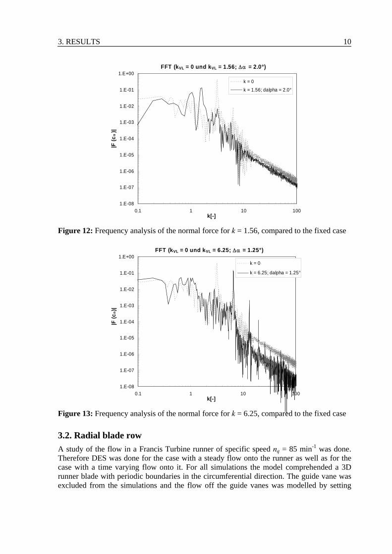
There can also be observed an effect on the frequency of the separation and therefore on the frequency of the blade normal forces in the second row. Fig. 12 and 13 show that the dominant frequency of the blade normal forces can be shifted to the pitching-frequency of the guide vanes. This effect could be utilized in cases where the frequency of the pressure fluctuations is about the eigenfrequency of a turbine, what could cause seriously damage.

3. RESULTS 9

Another positive effect is the reduction of the amplitudes of the fluctuations by pitching guide vanes, which is up to 25% regarding the maximum amplitudes as well as the mean amplitudes.

k = 0

k ≠ 0

Figure 11: Streamlines at a back blade; sequences. left: fixed case, instantaneous flow; right: pitching case, periodic averaged flow

3. RESULTS 10

FFT (kVL = 0 und kVL = 1.56; Δα = 2.0°)

1.E-08

1.E-07

1.E-06

1.E-05

1.E-04

1.E-03

1.E-02

1.E-01

1.E+00

0.1 1 10 100k[-]

|F (c

n )|

k = 0

k = 1.56; dalpha = 2.0°

Figure 12: Frequency analysis of the normal force for k = 1.56, compared to the fixed case

FFT (kVL = 0 und kVL = 6.25; Δα = 1.25°)

1.E-08

1.E-07

1.E-06

1.E-05

1.E-04

1.E-03

1.E-02

1.E-01

1.E+00

0.1 1 10 100k[-]

|F (c

n)|

k = 0

k = 6.25; dalpha = 1.25°

Figure 13: Frequency analysis of the normal force for k = 6.25, compared to the fixed case

3.2. Radial blade row A study of the flow in a Francis Turbine runner of specific speed nq = 85 min-1 was done. Therefore DES was done for the case with a steady flow onto the runner as well as for the case with a time varying flow onto it. For all simulations the model comprehended a 3D runner blade with periodic boundaries in the circumferential direction. The guide vane was excluded from the simulations and the flow off the guide vanes was modelled by setting

3. RESULTS 11

appropriate values for the inlet velocity. This simplification was justified as preliminary simulations of the guide vane – runner stage showed that there is a negligible gradient of the flow in the axial direction after the guide vanes. The flow rate was kept constant with Q/Qopt = 0.55. The effect of the guide vanes was modelled by the circumferential component of the inlet velocity cu0, which oscillated in the case of time varying flow. The oscillation was done in a way, that the mean cu was constant for all simulations and that the flow angle α(t) oscillated in a harmonic way.

3.2.1. Steady flow onto the runner The operating point Q/Qopt = 0.55 is in extreme part load. The angle of the absolute flow at the inlet is about 10.4°. This causes a very bad flow onto the runner blade, with a very high incidence angle near the crown, which gets smaller towards the band. Therefore a large separation at the leading edge occurs near the crown which extends to the band. At the band the flow with the smaller incidence angle turns the separation structure towards the trailing edge. The characteristic shape of the separation can be seen in Fig. 14, where the streamlines of the flow are plotted.

The large separation reduces the hydraulic efficiency of the runner which is 89.7%, compared to 94.3% in the optimum point of operation.

leading edge

trailing edge

crow

n

band

suctionsuction sideside

leading edge

trailing edge

crow

n

band

suctionsuction sideside

Figure 14: Separation on the suction side of the blade, visualized by the streamlines of the

flow

3. RESULTS 12

The flow in the studied operating point is very unstable and therefore highly transient. For the analysis the torque and the force were built as integral values, by integrating the local values over the entire blade surface. The values are of dimensionless form and are calculated as follows:

π

ωτ2

⋅= t (5)

Nr

Fc

b

f ⋅⋅⋅

=4

12

2ωρ

(6)

Nr

Mc

b

m ⋅⋅⋅

=5

12

2ωρ (7)

A frequency analysis of the torque coefficient is plotted in the Fig. 15. The figure shows a dominant peak at k = 5.4, the eigenfrequency of the separation.

FFT (k = 0)

1.E-14

1.E-12

1.E-10

1.E-08

1.E-06

1.E-04

1.E-02

0.1 1 10 100k [-]

|F(C

m)|

Figure 15: Frequency spectrum of the torque coefficient cm

3.2.2. Time varying flow onto the runner By exciting the flow via pitching the inlet angle of the flow, an improvement of the flow characteristics can be achieved. The hydraulic efficiency of the runner can be improved about a maximum of 0.5 percentage points at the parameter combination k = 0.92 and Δα = 0.25°. An improvement can be observed just in a small band of frequencies and amplitudes. Most combinations result in lower values of the efficiency. There is an amplitude Δα ~ 1.0° where the efficiency is nearly unaffected, independent of the frequency. It is a border for the angles, where a positive effect on the efficiency can be achieved, s. Fig. 16. At higher frequencies the efficiency tends towards the value of the

3. RESULTS 13

steady case. This is due to the fact, that the oscillation of the flow is damped towards the leading edge. The damping is affected by the frequency and the amplitude of the oscillation in a quadratic way and the oscillation is damped most at high frequencies and amplitudes.

0.8

0.82

0.84

0.86

0.88

0.9

0.92

0 2 4 6 8 10

k [-]

ηh

Δα=0.0°Δα=0.25°Δα=0.5°Δα=1.0°Δα=2.0°Δα=3.0°Δα=5.0°

Figure 16: Hydraulic efficiency depending on the excitation frequency

Similar to the flow in the tandem cascade, there is an influence on the frequency of the pressure fluctuations. This is shown in Figs. 17 to 20, where the spectra of the force and the torque coefficients for cases with excited flow are compared with the spectrum of the steady case. Due to the exciting of the flow, the peaks of the spectra are shifted exactly towards the exciting frequency. This can be observed for all studied parameters. Therefore in a Francis Turbine resonance effects can be avoided, by pitching the guide vanes and shifting the frequencies.

3. RESULTS 14

FFT (k = 0.46; Δα = 0.25°)

1.E-14

1.E-12

1.E-10

1.E-08

1.E-06

1.E-04

1.E-02

0.1 1 10 100k [-]

|F(C

f)|

k = 0

k = 0.46; dAlpha = 0.25°

Figure 17: Frequency spectrum of the cf for an excitation with k = 0.46 and Δα = 0.25°

FFT (k = 0.46; Δα = 0.25°)

1.E-14

1.E-12

1.E-10

1.E-08

1.E-06

1.E-04

1.E-02

0.1 1 10 100k [-]

|F(C

m)|

k = 0

k = 0.46; dAlpha = 0.25°

Figure 18: Frequency spectrum of cm for an excitation with k = 0.46 and Δα = 0.25°

3. RESULTS 15

FFT (k = 0.92; Δa = 0.25°)

1.E-14

1.E-12

1.E-10

1.E-08

1.E-06

1.E-04

1.E-02

0.1 1 10 100k [-]

|F(C

f)|

k = 0

k = 0.92; dAlpha = 0.25°

Figure 19: Frequency spectrum of cf for an excitation with k = 0.92 and Δα = 0.25°

FFT (k = 0.92; Δα = 0.25°)

1.E-14

1.E-12

1.E-10

1.E-08

1.E-06

1.E-04

1.E-02

0.1 1 10 100k [-]

|F(C

m)|

k = 0

k = 0.92; dAlpha = 0.25°

Figure 20: Frequency spectrum of cm for an excitation with k = 0.92 and Δα = 0.25°

Another positive effect is shown in Figs. 21 and 22, where the rms amplitudes of the time variing torques and axial forces are plotted. The values are set relative to the amplitudes in the nonpitching case. The plots for the maximum amplitudes are not shown here, but they are very similar to the rms plots. The minimum amplitudes in all figures is at k = 5.4, which is the eigenfrequency of the separation. The rms fluctuations of the torque can maximally be lowered about 20.4% at Δα = 3.0° and the maximum fluctuations about 15.1% at the same value. The rms fluctuations of the axial force can be reduced about 32.9° at Δα = 1.0° and

3. RESULTS 16

the maximum fluctuations about 28.1% at Δα = 3.0°. At higher frequencies the amplitudes tend towards the values of the steady case. This is due to the damping of the oscillation which was described above.

ΔM - rms

0.0

0.5

1.0

1.5

2.0

2.5

0 2.5 5 7.5 10

k [-]

A(k

) / A

(k=0

)Δα = 0.0°Δα = 0.25°Δα = 0.5°Δα = 1.0°Δα = 1.5°Δα = 3.0°Δα = 5.0°

Figure 21: rms amplitudes of the torque

ΔFax - rms

0.0

0.5

1.0

1.5

2.0

2.5

0 2.5 5 7.5 10

k [-]

A(k

) / A

(k=0

)

Δα = 0.0°Δα = 0.25°Δα = 0.5°Δα = 1.0°Δα = 1.5°Δα = 3.0°Δα = 5.0°

Figure 22: rms amplitudes of the axial force

4. SUMMARY 17

4. SUMMARY

The simulations of the translational tandem cascade showed that guide vanes, pitching with appropriate frequencies and amplitudes, could reduce the total pressure drop in radial turbines. In extreme part and overload conditions this can increase the efficiency of the turbine. The simulations of the radial runner confirmed this although the effect is smaller than in the tandem cascade. In Francis Turbines with lower specific speed the effect can be expected to be more distinctive.

Furthermore a positive effect regarding the pressure fluctuations can be noticed. The fluctuations of the blade forces can be reduced, which would result in a remarkable increase of the lifespan of turbines.

It is also possible to shift the frequency of the pressure fluctuations towards the frequency of the pitching guide vanes. This can be useful in operation points where the pressure fluctuations could stimulate the turbine at its eigenfrequency.

REFERENCES

[1] ISSA, R.I., 1986, „Solution of implicitly discretized fluid flow equations by operator-splitting”, Journal of Computational Physics, Vol. 62, p. 40-65

[2] FERZIGER, J.H., AND PERIC, M., 2002, Computational Methods for Fluid Dynamic, Springer, Berlin Heidelberg

[3] WUNDERER, R., 2007, „Algebraischer Algorithmus für die Netzdeformierung”, report, Institute of Fluid Mechanics, Technische Universität München [4] WUNDERER, R., 2007, „Aktive Strömungsbeeinflussung”, Abschlußberichtbericht zum Projekt KW21 [5] PIOMELLI, U., AND BALARAS, E., 2002, „Wall-Layer Models for Large-Eddy Simulations”, Annual Review of Fluid Mechanics Vol. 34, p. 349-374

[6] SPALART, P. R., JOU, W. H., STRELETS, M., AND ALLMARAS, S. R., 1997, „Comments on the feasibility of LES for wings, and on a hybrid RANS/LES approach”, 1st AFOSR Int. Conf. on DNS/LES, Aug. 4-8, 1997, Ruston, LA. In: Advances on DNS/LES, C. Liu and Z. Liu Eds., Greyden Press, Columbus, OH, USA

[7] STRELETS, M., 2001, „Detached Eddy Simulation of Massively Separated Flows”, AIAA Paper 2001-0879

[8] MENTER, F. R., AND KUNTZ, M., 2004, „Development and application of a zonal DES turbulence model for CFX-5”, ANSYS CFX Validation Report

[9] SPALART, P. R., DECK, S., SHUR, M. L., SQUIRES, K. D., STRELETS, M. KH., AND TRAVIN, A., 2006, „A new version of detached-eddy simulation, resistant to ambiguous grid densities”, Theor. Comput. Fluid Dyn. (2006) 20: 181-195

[10] WUNDERER, R. ; SCHILLING, R., 2008, „Numerical Simulation Of Active Flow Control In Hydro Turbines”, ISROMAC-12 : 12th International symposium on transport phenomena and dynamics of rotating machinery

REFERENCES 18

[11] MENTER, F. R., AND EGOROV, Y., 2005, „A scale-adaptive simulation model using two-equation models”, AIAA Paper 2005-1095

[12] TRAVIN, A., SHUR, M., STRELETS, M., AND SPALART, P.R., 2000, „Physical and numerical upgrades in the detached-eddy simulation of complex turbulent flows”, Proceedings of the Euromech Colloquium on LES of Complex transitional and turbulent flows, Munich, Oct. 2000

[13] WUNDERER, R. ; SCHILLING, R., 2008, „The Study Of Active Flow Control In Francis Turbines”, IAHR 2008, 24th Symposium on Hydraulic Machinery and Systems

[14] WERDECKER, F., 2000, „Strömungswechselwirkung an einem Tandemgitter mit schwingender Vorleitschaufel”, Dissertation Technische Universität München

[15] PIZIALI, R. A., 1994, „2-D and 3-D Oscillating Wing Aerodynamics for a Range of Angles of Attack Including Stall”, NASA Technical Memorandum 4632

[16] LEDER, A., 1992, Abgelöste Strömungen Physikalische Grundlagen, Vieweg, Braunschweig/Wiesbaden