UNIVERSITA’ DEGLI STUDI DI PADOVA

DEPARTMENT OF INDUSTRIAL ENGINEERING

MASTER DEGREE COURSE IN ELECTRICAL ENGINEERING

MASTER THESIS

“Numerical Models for Induction Hardening of Gears”

SUPERVISOR: Prof. Fabrizio Dughiero

CO-EXAMINER: Eng. Mattia Spezzapria

Prof. Philippe Bocher (ETS, Montréal)

GRADUATE: Damiano Mingardi

SESSION 2012/2013

I

II

III

Ringraziamenti

Nel mio cammino verso la conclusione del lungo periodo da studente universitario ci sono state

alcune persone che per me sono state di fondamentale importanza non solo per quanto riguarda

aiuto fisico o morale, ma anche solo per la loro splendida presenza.

Voglio pertanto ringraziare dinanzi tutto i miei genitori, che hanno sempre creduto nelle mie

capacità e che hanno sempre saputo darmi buoni consigli in questo impegnativo periodo della mia

vita.

Un grazie particolare va anche a tutta la famiglia Perin, composta da persone con dei valori davvero

inestimabili, che mi è sempre stata vicino.

Un grazie va anche a tutti i miei amici e in particolare Alberto e Alberto, da sempre compagni

d’avventure.

Voglio ricordare anche il maestro Pierluigi che mi ha visto impegnato nelle sfide tra le più grandi

della mia vita, ed è anche grazie ai suoi insegnamenti che sono arrivato fino a questo traguardo.

Grazie anche a coloro che mi hanno permesso di svolgere questa Tesi: in primis il professor

Fabrizio Dughiero, ma anche Mattia per i suoi innumerevoli consigli e il professor Philippe Bocher,

che mi ha allegramente accolto e guidato nel periodo trascorso a Montréal.

IV

V

NUMERICAL MODELS FOR INDUCTION HARDENING OF GEARS

Damiano Mingardi

SUMMARY

Nowadays, induction heat treatment processes are increasingly used in aeronautics and

automotive to improve the service performance of several mechanical components such as

gears. With induction, heating can be localized to the specific areas where metallurgical changes are

desired. For example, in contrast to carburising and nitriding, induction hardening does not require

heating of the whole gear and the heating effect on adjacent areas is minimum. Furthermore by its

selective heating, the process can produce residual compressive stresses favorable to the fatigue

behavior without generating excessive distortion.

The heating and the quenching rate affect the final microstructure of the workpiece, and the case

depth generated are machine dependent parameters (frequency, power, preheating and heating

times, design of the coil etc). At the current state of the art there are several numerical models able

to predict the temperature distribution during the heating process. They allow the designers to avoid

a trial and error approach, that is costly and time consuming, to establish the parameters for the

induction heating process. Due to the complexity of the phenomena involved in the induction

hardening process, in numerical models it is necessary to introduce simplifications such as in the

description of the material’s properties. These simplifications may lead to errors and substantial

differences between the models and the real process of induction hardening. Nevertheless there are

no studies in literature that analyze the accuracy of these methods by comparing them with

experimental measurements.

Therefore, this thesis involves a study of sensitivity of the hardness profile of a gear heated by

induction using finite element method (FEM) software, and it proposes a comparison with

experimental measurements of superficial temperature, that is a necessary step towards the

development of prediction models.

This study aims at evaluating the effect of machine parameters (frequency, coil dimensions and the

presence of a flux concentrator over and below the gear) in order to obtain a homogeneous hardened

profile both in the tip and in the tooth of the gear, and to prevent the entire tooth from being

austenitised. In particular it is supposed that the flux concentrator has a key role in reducing the

edge effect, otherwise difficult to control. In addition a robust method for the measurement of

surface temperature fields during fast induction heating treatment is chosen for the comparison to

the isotherm obtained by numerical models. It is based on the coupling of temperature indicating

VI

lacquers and a high speed camera system, that allows to extract the temporal evolution of the 816°C

and 927°C isotherms. Models with different approximation of the material’s properties are

proposed, in order to understand their effect on the isotherm’s evolution. In addition a comparison

between the edge effect estimated by the simulations and the actual one has been proposed by

observing the hardened layer.

Keywords: Validation, induction hardening, numerical models, simulation, sensitivity study,

experimental, gear, isotherm

VII

NUMERICAL MODELS FOR INDUCTION HARDENING OF GEARS

Damiano Mingardi

Sommario

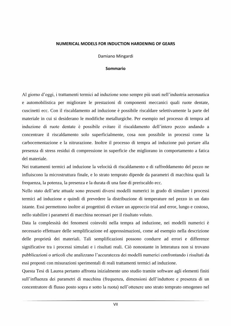
Al giorno d’oggi, i trattamenti termici ad induzione sono sempre più usati nell’industria aeronautica

e automobilistica per migliorare le prestazioni di componenti meccanici quali ruote dentate,

cuscinetti ecc. Con il riscaldamento ad induzione è possibile riscaldare selettivamente la parte del

materiale in cui si desiderano le modifiche metallurgiche. Per esempio nel processo di tempra ad

induzione di ruote dentate è possibile evitare il riscaldamento dell’intero pezzo andando a

concentrare il riscaldamento solo superficialmente, cosa non possibile in processi come la

carbocementazione e la nitrurazione. Inoltre il processo di tempra ad induzione può portare alla

presenza di stress residui di compressione in superficie che migliorano in comportamento a fatica

del materiale.

Nei trattamenti termici ad induzione la velocità di riscaldamento e di raffreddamento del pezzo ne

influiscono la microstruttura finale, e lo strato temprato dipende da parametri di macchina quali la

frequenza, la potenza, la presenza e la durata di una fase di preriscaldo ecc.

Nello stato dell’arte attuale sono presenti diversi modelli numerici in grado di simulare i processi

termici ad induzione e quindi di prevedere la distribuzione di temperature nel pezzo in un dato

istante. Essi permettono inoltre ai progettisti di evitare un approccio trial and error, lungo e costoso,

nello stabilire i parametri di macchina necessari per il risultato voluto.

Data la complessità dei fenomeni coinvolti nella tempra ad induzione, nei modelli numerici è

necessario effettuare delle semplificazione ed approssimazioni, come ad esempio nella descrizione

delle proprietà dei materiali. Tali semplificazioni possono condurre ad errori e differenze

significative tra i processi simulati e i risultati reali. Ciò nonostante in letteratura non si trovano

pubblicazioni o articoli che analizzano l’accuratezza dei modelli numerici confrontando i risultati da

essi proposti con misurazioni sperimentali di reali trattamenti termici ad induzione.

Questa Tesi di Laurea pertanto affronta inizialmente uno studio tramite software agli elementi finiti

sull’influenza dei parametri di macchina (frequenza, dimensioni dell’induttore e presenza di un

concentratore di flusso posto sopra e sotto la ruota) nell’ottenere uno strato temprato omogeneo nel

VIII

dente e nella cava di una ruota dentata temprata ad induzione, evitando l’austenitizzazione di tutto il

dente. In particolare si suppone che l’uso del concentratore di flusso abbia un ruolo chiave nella

riduzione dell’ effetto di bordo.

Successivamente è stato proposto un confronto tra i risultati di misure sperimentali di temperatura

su un processo di tempra e i risultati delle simulazioni numeriche dello stesso processo. Per le

misure sperimentali si è scelto di utilizzare speciali vernici termiche che tendono a trasformarsi

visibilmente al raggiungimento di una determinata temperatura. Filmando il processo di tempra con

una telecamera ad alta velocità di acquisizione è stato possibile risalire all’evoluzione temporale

delle isoterme a 816°C e 927°C. Sono stati proposti modelli con diverse approssimazioni delle

proprietà dei materiali, allo scopo di capirne l’influenza sull’evoluzione delle isoterme. Inoltre è

stato proposto anche un confronto tra l’effetto di bordo stimato dalle simulazioni e quello reale

osservando la profondità dello strato temprato.

Parole chiave: Validazione, tempra ad induzione, modelli numerici, simulazioni, misurazioni

sperimentali, isoterme, ruote dentate

IX

1. INDUCTION HARDENING .................................................................................................................................... 1

1.1 INTRODUCTION ...................................................................................................................................................... 1

1.2 THE ELECTROMAGNETIC PROBLEM ............................................................................................................................. 1

1.2.1 Theoretical background ................................................................................................................................ 1

1.2.2 Basics electromagnetic phenomena in induction heating ............................................................................ 4 1.2.2.1 Skin effect ..............................................................................................................................................................4 1.2.2.2 Electromagnetic proximity effect ..........................................................................................................................6 1.2.2.3 Electromagnetic ring effect ...................................................................................................................................6

1.3 THE THERMAL PROBLEM .......................................................................................................................................... 7

1.3.1 Conduction .................................................................................................................................................... 8

1.3.2 Convection .................................................................................................................................................... 8

1.3.3 Irradiance ...................................................................................................................................................... 9

1.4 MATERIAL’S PROPERTIES .......................................................................................................................................... 9

1.4.1 Electrical properties ...................................................................................................................................... 9 1.4.1.1 Electrical conductivity ..........................................................................................................................................10 1.4.1.2 Relative magnetic permeability ...........................................................................................................................10

1.4.2 Thermal properties ...................................................................................................................................... 11 1.4.2.1 Thermal conductivity ...........................................................................................................................................11 1.4.2.2 Specific heat.........................................................................................................................................................11

1.5 METALLURGICAL ANALYSIS OF MARTENSITIC HARDENING ............................................................................................. 11

1.5.1 Austenitization and hardening .................................................................................................................... 11

1.5.2 Quenching ................................................................................................................................................... 15

1.5.3 Retained austenite ...................................................................................................................................... 19

1.5.4 Tempering ................................................................................................................................................... 21

1.5.5 The hardened profile ................................................................................................................................... 22

1.5.6 Residual stresses ......................................................................................................................................... 23

1.6 POWER SUPPLIES FOR INDUCTION HEAT TREATMENT.................................................................................................... 25

1.6.1 Power supplies ............................................................................................................................................ 26 1.6.1.1 AC to DC rectifier .................................................................................................................................................28 1.6.1.2 DC to AC inverter .................................................................................................................................................29

1.6.2 Load matching ............................................................................................................................................ 33

1.6.3 Process control ............................................................................................................................................ 34

2. THE GEARS AND AISI 4340’S PROPERTIES ..........................................................................................................37

2.1 INTRODUCTION .................................................................................................................................................... 37

2.2 TEST CASE 1 ........................................................................................................................................................ 38

2.3 TEST CASE 2 ........................................................................................................................................................ 38

2.4 AISI 4340 .......................................................................................................................................................... 39

2.4.1 Relative magnetic permeability .................................................................................................................. 40

2.4.2 Specific heat ................................................................................................................................................ 41

2.4.3 Electrical conductivity ................................................................................................................................. 42

2.4.4 Thermal conductivity................................................................................................................................... 42

3. NUMERICAL MODELING OF THE PROCESS .........................................................................................................45

3.1 INTRODUCTION .................................................................................................................................................... 45

X

3.2 BUILDING OF THE GEOMETRY .................................................................................................................................. 47

3.3 BUILDING OF THE MESH ......................................................................................................................................... 48

3.4 DESCRIPTION OF MATERIALS AND THEIR PROPERTIES .................................................................................................... 50

3.5 DESCRIPTION OF THE PROBLEM AND OF THE BOUNDARY CONDITIONS .............................................................................. 52

3.6 COMPUTATION AND POST PROCESSING OF THE RESULTS ............................................................................................... 54

4. OPTIMIZATION OF INDUCTION HARDENING PARAMETERS ...............................................................................56

4.1 INTRODUCTION .................................................................................................................................................... 56

4.2 INFLUENCE OF FLUX CONCENTRATOR ........................................................................................................................ 56

4.3 INFLUENCE OF INDUCTOR’S DIMENSIONS ................................................................................................................... 60

4.4 INFLUENCE OF THE FREQUENCY AND THE DURATION ON MF PREHEATING PHASE ............................................................... 62

4.5 CONCLUSIONS ...................................................................................................................................................... 67

5. VALIDATION OF NUMERICAL MODELING ..........................................................................................................69

5.1 INTRODUCTION .................................................................................................................................................... 69

5.2 ANALYSIS OF EXPERIMENTAL PROCEDURE .................................................................................................................. 69

5.3 NUMERICAL SIMULATION ....................................................................................................................................... 71

5.4 COMPARISON BETWEEN EXPERIMENTAL AND NUMERICAL RESULT: ISOTHERM’S EVOLUTION ................................................ 74

5.5 COMPARISON BETWEEN EXPERIMENTAL AND NUMERICAL RESULTS: THE EDGE EFFECT ........................................................ 86

5.6 CONCLUSIONS: .................................................................................................................................................... 89

6. CONCLUSION .....................................................................................................................................................91

BIBLIOGRAPHY ..........................................................................................................................................................94

XI

XII

1

1. Induction hardening

1.1 Introduction

Nowadays, induction heat treatment processes such as induction hardening are increasingly used in

automotive and aeronautics to improve the service performances such as fatigue life, resistance at

usury and plastic deformation of various mechanical components.

Induction hardening is a reliable and time-saving process, as it takes few seconds to take place, due

to higher specific power of the process. Moreover heating can be localized to the specific areas

where metallurgical changes are desired (e.g., flank, root and gear tip can be selectively hardened)

and the heating effect on adjacent areas is minimum.

Last but not least, an induction system improves working conditions for employees and reduces

pollution by eliminating smoke, waste heat, noxious emissions and loud noise. Heating is safe and

efficient with no open flame to endanger the operator or obscure the process.

1.2 The electromagnetic problem

1.2.1 Theoretical background

In electrical engineering practice, the simulation of devices, measuring arrangements and various

electrical equipments is based on Maxwell’s equations coupled with the constitutive relations.

The Maxwell equations are the set of four fundamental equations governing electromagnetism,

which can be used in the frame of any numerical field analysis tool, e.g. in the finite element

method.

The field quantities are depending on space r and on time t, therefore in the following, a shorter

notation will be used. For example we have that magnetic field intensity .

These equations, written in differential vector form, are:

1.

2.

2

3.

4.

Where the first equation is the gauss’s law for magnetism, that states that the divergence of the

vector magnetic flux density is equal to zero. In other words, is a solenoidal vector field.

Free magnetic charges do not exist physically and magnetic flux lines close upon themselves.

The second equation is the electric Gauss's law. It describes the relationship between an electric

field and the electric charges that cause it. The source of electric field is the electric charge and

electric flux lines start and close upon the charge. is electric flux density, and

is the free electric charge density.

The third equation is called Faraday's law and demonstrates that each variation of magnetic flux

density produces an electric field intensity .

The fourth and last equation is Ampère-Maxwell’s law, that states that magnetic field intensity

can be generated by an electrical current ( is the conduction current density)

and by the so called displacement current in dielectric media, which is generated by a time-varying

electric field.

In order to Maxwell's equations to be definite it is necessary to specify the constitutive relations of

materials that are, for a linear, isotropic medium:

Where is the relative permittivity of the material, is the magnetic permeability, and is the

electric conductivity of the material. The constant is the permeability of

vacuum and is the permittivity of free space

The Maxwell equations can be rearranged in the case of induction heating, in which frequencies

remain below 10 MHz [4].

Indeed, in this case it is possible to neglect the terms

on the Ampere-Maxwell equation

that becomes

3

1)

Moreover, after some vector algebra and by replacing the latter constitutive equation in the third

Maxwell law, we obtain

2)

The Faraday’s law can also be expressed remembering that is solenoidal and hence we can write

, where is the magnetic vector potential. We have

3)

That integrated gives

4)

Where is the electric scalar potential. By multiplying 4) for , we have

5)

Where is the source current density in the induction coil. 5) states that the total current

density is given by eddy currents and the current imposed in the inductor.

By replacing the second constitutive equation and 3) in 2), neglecting the hysteresis and magnetic

saturation we have

And hence

That, remembering the equation 5), becomes

6)

Where is the angular frequency. Equation 6) is the potential vector formulation.

For the great majority of induction heating processes such as hardening a heat effect due to

hysteresis losses does not exceed 7% compared to the heat effect due to eddy current losses [4]. So

in these case neglecting hysteresis is quite valid.

One of the major difficulties in electromagnetic field and heat transfer computation is the

nonlinearity of material properties, as clarified subsequently. So, using simple analytical methods

that cannot take into account the variation of these properties could lead to unpredictable and

erroneous results. Moreover, the geometries of the coil and the workpiece are often very complex.

For these reasons, modern induction heat treatment specialists turns to highly effective numerical

4

methods such as finite element method, that are widely and successfully used in the computation of

electromagnetic and heat transfer problems in heat treatment.

1.2.2 Basics electromagnetic phenomena in induction heating

Induction heating is the process of heating an electrically conducting object by electromagnetic

induction, where eddy currents (also called Foucault currents) are generated within the material by

electromagnetic forces, according to the third Maxwell’s equation, and resistance leads to Joule

heating of the metal.

Fig. 1.1 Simple scheme of induction heating process: a) coil, b) load, c) magnetic field lines

By several electromagnetic effects such as skin effect, proximity effect and ring effect current

distribution in the coil and in the load is not uniform.

1.2.2.1 Skin effect

Skin effect is the tendency of an alternating electric current to become distributed within

a conductor such that the current density is largest near the surface of the conductor, and decreases

with greater depths in the conductor, following the formula:

5

Where is the current density at the surface and δ is called skin depth. Skin depth is defined as the

depth below the surface of the conductor at which the current density has fallen to 1/e of . In

normal cases it is well approximated as:

Where ρ is the resistivity of the conductor, ω is the angular frequency of current and is the

relative magnetic permeability of the conductor. Approximately 86 % of the power will be

concentrated in the first penetration depth.

It is necessary to mention that penetration depth is not constant during the induction heating

process. Indeed the value of relative magnetic permeability has a nonconstant distribution within the

workpiece and moreover it changes with the temperature of the material and the magnetic field.

The skin effect causes the effective resistance of the conductor to increase at higher frequencies,

where the skin depth is smaller, thus reducing the effective cross-section of the conductor. The skin

effect is due to opposing eddy currents induced by the changing magnetic field resulting from the

alternating current.

Power distribution, related to current density, follows the law:

Where w is the power density in the sample and is the power density at the surface.

Fig. 1.2 Current and power density distribution in a square sample heated by induction.

6

1.2.2.2 Electromagnetic proximity effect

A changing magnetic field will influence the distribution of an electric current flowing within

an electrical conductor, by electromagnetic induction. When an alternating current flows through an

isolated conductor, it creates an associated alternating magnetic field around it. The alternating

magnetic field induces eddy currents in adjacent conductors, altering the overall distribution of

current flowing through them. The result is that the current is concentrated in the areas of the

conductor furthest away from nearby conductors carrying current in the same direction. Current

distribution is concentrated on the neighbor side of conductors if they are carrying current in the

opposite direction.

Fig. 1.3 proximity effect

1.2.2.3 Electromagnetic ring effect

Up to now we discussed current density distribution in straight conductors. If a conductor is bent to

shape it into a ring, then its current will be redistributed as shown in figure 1.4.

7

Fig. 1.4 ring effect.

Magnetic flux lines will be concentrated inside the ring and therefore the density of the magnetic

field will be higher inside the ring. As a result, the majority of the current will flow within the thin

inside surface layer of the ring.

The presence of ring effect can have a positive effect in induction heating of cylinder for example.

Indeed, where the workpiece is located inside the induction coil, the combination of ring effect and

skin and proximity effects will leads to a concentration of the coil current on the inside diameter of

the coil. As a result, there will be close coil-workpiece coupling, which leads to good coil

efficiency.

1.3 The thermal problem

In the design of a induction heating system it is very important to know precisely heating time and

power necessary to obtain a determined temperature’s profile needed for the process.

Moreover, due to the consideration explained in previous chapter, a typical specific power

distribution of an induction heating process is not constant. For these reasons we need to know the

thermal transient in the workpiece.

8

All the three heating transfer methods are important for induction heating processes: so it is useful

to describe equations that settle thermal balance.

1.3.1 Conduction

The heat generated by the induced currents in the workpiece flows by conduction from hot regions

to cold heart of the piece. The basic law which describes the transfer of heat by conduction is

Fourier's law.

Where is the heat flux by conduction , k is thermal conductivity

and T is

temperature [K]. According to Fourier’s law, the greater is the temperature’s difference between the

surface and the core, the greater is .

1.3.2 Convection

During the induction heat treatment, part of the heat generated is lost toward the surrounding

environment by convection. Convection is carried out by fluid and Newton's law states that the rate

of convective heat transfer is directly proportional to the difference between the surface temperature

of the workpiece and the fluid surrounding it.

)

Where is the density of heat lost by convection is the coefficient of heat loss by

convection

, Ts is the surface temperature [K] of the workpiece and is the temperature of

the fluid of the environment [K].

The coefficient of heat loss by convection depends on the thermal properties of the material and

part of the surrounding fluid , the inductor, the viscosity of the fluid and the speed of rotation of the

workpiece during heating. In fact, convection is considered forced regime and not free because the

parts are rotated or displaced during heating. In practice we will use the so called differential curves

of speed quenching in order to describe the quenching phase.

9

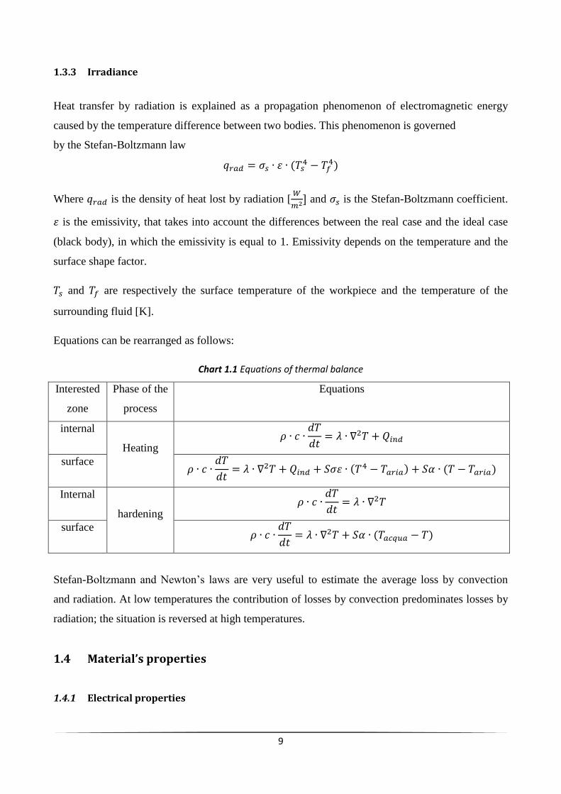
1.3.3 Irradiance

Heat transfer by radiation is explained as a propagation phenomenon of electromagnetic energy

caused by the temperature difference between two bodies. This phenomenon is governed

by the Stefan-Boltzmann law

Where is the density of heat lost by radiation [

and is the Stefan-Boltzmann coefficient.

is the emissivity, that takes into account the differences between the real case and the ideal case

(black body), in which the emissivity is equal to 1. Emissivity depends on the temperature and the

surface shape factor.

and are respectively the surface temperature of the workpiece and the temperature of the

surrounding fluid [K].

Equations can be rearranged as follows:

Chart 1.1 Equations of thermal balance

Interested

zone

Phase of the

process

Equations

internal

Heating

surface

Internal

hardening

surface

Stefan-Boltzmann and Newton’s laws are very useful to estimate the average loss by convection

and radiation. At low temperatures the contribution of losses by convection predominates losses by

radiation; the situation is reversed at high temperatures.

1.4 Material’s properties

1.4.1 Electrical properties

10

The electromagnetic properties more involved in induction hardening processes are relative

magnetic permeability and electrical conductivity.

1.4.1.1 Electrical conductivity

The electrical conductivity (σ) expressed in Siemens per meter

measures the capacity of a

material to conduct an electrical current. Generally, metallic materials are considered good

electrical conductors compared to insulating materials.

This electrical property corresponds to the inverse of the electrical resistivity and it depends on the

temperature. Conductivity trend as function on temperature can be approximated as linear,

according to the relation:

In which is the resistivity of the material at 0 ° C, while is a coefficient to increase the

resistivity with temperature.

However, this approximation may differ from the actual behavior. For example, in carbon steel one

can observe that conductivity varies in a nonlinear way, decreasing approximately five times in the

range 0-800 ° C, while at 1200-1300 ° C it is approximately seven times less than the one measured

at room temperature.

1.4.1.2 Relative magnetic permeability

The relative magnetic permeability indicates the capacity of the material to conduct a magnetic

flow compared to vacuum and it is a complex function of the magnetic field and temperature.

While in non magnetic materials is equal to 1, in magnetic material it starts from the value of the

permeability at 20 ° C ( , varies a little increasing temperature, and collapses to unit value

reaching the Curie temperature of the material, becoming diamagnetic.

11

1.4.2 Thermal properties

Thermal properties involved in induction hardening processes are thermal conductivity and specific

heat.

1.4.2.1 Thermal conductivity

Thermal conductivity defines the rate at which a heat flow is transmitted by conduction in the

materials in function of time.

In the case of induction hardening of gears we have to remember that steel has rather high thermal

conductivity, so heat generated in a thin region in the surface is rapidly transferred to the cold heart

of the piece and hence, it becomes difficult to control heat generated in the surface. This especially

applies to the root of the gear.

Thermal conductivity is function of temperature and heating rate.

1.4.2.2 Specific heat

The specific heat corresponds to the amount of heat required to increase of 1°C the mass unit, kg.

This property is also a complex function of temperature and heating rate.

Specific heat of steel increases linearly with temperature until the temperature of the beginning of

austenitization (Ac1). After that it reaches rapidly the peak of

at a temperature between

Ac1 and Ac3, and then it decreases drastically before reaching Ac3. This behavior is due to the

latent heat of phase transformation.

1.5 Metallurgical analysis of martensitic hardening

1.5.1 Austenitization and hardening

The austenitizing process is an extremely delicate phase in the process of induction hardening.

12

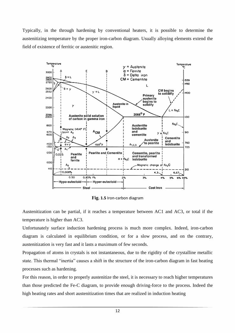
Typically, in the through hardening by conventional heaters, it is possible to determine the

austenitizing temperature by the proper iron-carbon diagram. Usually alloying elements extend the

field of existence of ferritic or austenitic region.

Fig. 1.5 Iron-carbon diagram

Austenitization can be partial, if it reaches a temperature between AC1 and AC3, or total if the

temperature is higher than AC3.

Unfortunately surface induction hardening process is much more complex. Indeed, iron-carbon

diagram is calculated in equilibrium condition, or for a slow process, and on the contrary,

austenitization is very fast and it lasts a maximum of few seconds.

Propagation of atoms in crystals is not instantaneous, due to the rigidity of the crystalline metallic

state. This thermal “inertia” causes a shift in the structure of the iron-carbon diagram in fast heating

processes such as hardening.

For this reason, in order to properly austenitize the steel, it is necessary to reach higher temperatures

than those predicted the Fe-C diagram, to provide enough driving-force to the process. Indeed the

high heating rates and short austenitization times that are realized in induction heating

13

treatments affect the microstructure of the austenite immediately prior to quenching.

Choosing the proper treatment temperature is possible by using CHT diagrams, or "Continuous-

Heating-Transformation".

Fig. 1.6 CHT diagram for C60 steel

In determination of austenitizing temperature the prior metallurgical structure is also very

important. Indeed the more cementite carbides are dispersed, the lower is the temperature

necessary to obtain homogeneous austenite.

Fig. 1.7 Influence of prior microstructure on starting austenitization temperature

14

When discussing induction hardening, it is imperative to mention the importance of having

“favourable” material conditions prior to gear treatment. Hardness repeatability and the stability of

the hardness pattern are grossly affected by the consistency of the microstructure prior to heat

treatment and the steel’s chemical composition.

A good initial microstructure, comprising a homogeneous fine-grained quenched and tempered

structure leads to fast and consistent response to induction heat treating, with the

smallest shape/size distortion and a minimum amount of grain growth. This type of prior

microstructure results in higher hardness and deeper hardened case depth compared to a

ferritic/pearlitic initial microstructure.

Having a good microstructure improves also mechanical characteristics of the core, especially

fatigue resistance.

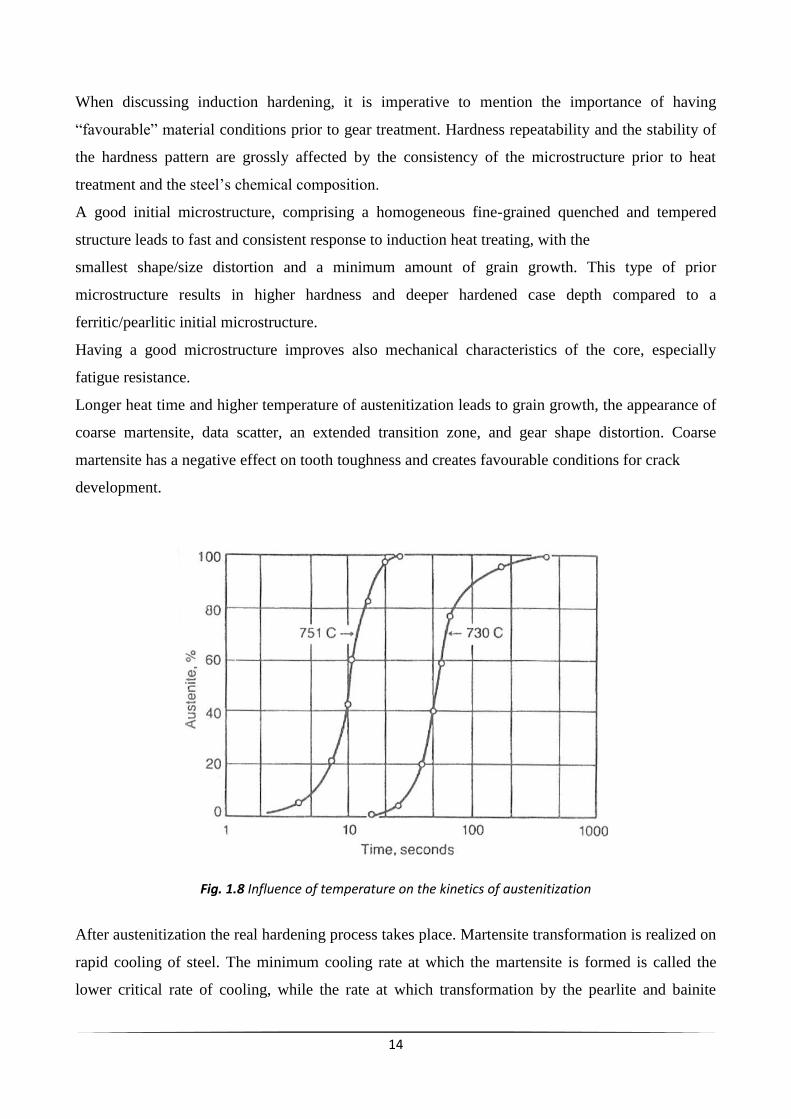
Longer heat time and higher temperature of austenitization leads to grain growth, the appearance of

coarse martensite, data scatter, an extended transition zone, and gear shape distortion. Coarse

martensite has a negative effect on tooth toughness and creates favourable conditions for crack

development.

Fig. 1.8 Influence of temperature on the kinetics of austenitization

After austenitization the real hardening process takes place. Martensite transformation is realized on

rapid cooling of steel. The minimum cooling rate at which the martensite is formed is called the

lower critical rate of cooling, while the rate at which transformation by the pearlite and bainite

15

mechanism are suppressed completely is referred to as the upper critical rate of cooling or

quenching. The upper critical rate of cooling can be determined through CCT diagrams

(Continuous-Cooling-Transformation).

Fig. 1.9 CCT diagrams

1.5.2 Quenching

The main purpose of the quench, however applied, is to remove the heat from the part as rapidly as

possible while minimizing any stresses that may occur in the process.

We consider for the moment that quenching is done by soaking the workpiece in a liquid bath

without agitation, immediately after induction heating.

Cooling rate is not constant but varies as a function of the surface temperature of the workpiece.

16

Fig. 1.10 The three stages of cooling

The three stages of the quenching process are:

1. Calefaction: in this stage a steam barrier is formed around the material, causing a minimal

heat transfer and therefore a slower cooling. Indeed the coolant fluid is not in direct contact

with the material. This behavior is called the Leidenfrost effect. It appears when the

workpiece temperature is much higher than the liquid one.

2. Boiling: decreasing workpiece’s temperature, the film of steam gradually decreases in

thickness until the fluid touches it’s hot surface. In this stage heat transfer is maximum.

3. Convection: The temperature of the surface of the workpiece falls below the liquid’s

saturation temperature, ending the boiling’s stage. Heat transfer is smaller.

Nevertheless, this subdivision represent just a qualitative information about quenching

phenomena, because of the multitude of factors involved. For example, especially for induction

hardening, quenching speed is not the same throughout the material, and a big amount of heat

flows towards the cold heart of the piece.

Quenching phase determines the final properties of the treated material and it is critical for

residual stresses distribution during the process. So it is necessary to take into account some

criteria in choosing the coolant fluid:

The length of the film-boiling phase must be sufficiently short so that the steel can be

hardened and not so long so that the cooling process would extend into the ferrite-

pearlite transformation region of the steel.

The cooling rate value must be sufficiently high through the nose of the ferrite-pearlite

transformation region, which is typically approximately 500-600 °C for many steels, to

minimize the potential formation of these transformation product.

17

The nucleate boiling to convective cooling transformation temperature should be as low

as possible to achieve maximum hardening potential.

In the convective region, cooling should be sufficiently low in order to avoid distortion

and /or cracking. Quench cracking is caused by the formation of stresses within the part

due to the normal contraction of the metal as it is cooled. In addition, microstructural

stresses also occur as the steel expands with the formation of martensite.

The quenching media in general use are :

Water: it is probably the most widely quenchant fluid used as it is simple and effective.

Cold water is one of the most severe of the quenchants, and rapid agitation allows it to

approach the maximum capabilities of the liquid quenchants. It cools at the rate of 982°C per

second. It tends, however, to form bubbles on the surface of the metal being quenched and

causes soft spots. Furthermore, cooling rate in martensitic transformation region is very

high, causing the formation of cracks and distortions, so a brine solution is often used to

prevent this trouble.

Fig. 1.11 Effect of temperature on quenching properties of water

Brine: Brine cooling rates are the most rapid of all the quenchants. While steam breakdown

is extremely rapid, higher cooling rates may increase the possibility of distortion, and

quench cracking of the part may occur. Brine quenching can eliminate soft spots where the

part geometry permits rapid quenching. This rapid quenching action is caused by minute salt

crystals that are deposited on the surface of the work. Localized high temperatures cause the

crystals to fragment violently, creating turbulence that destroys the vapor phase. A 10%

solution of NaCl is usually an effective quench. The relationship of brine concentration to

hardness is shown in figure 1.12. Number above curve indicates distance from quenched end

in units of 1/16 inch. Small variations in quench temperature will not greatly affect the

18

cooling rate of the system. A temperature of 20˚C assures maximum effectiveness of

cooling.

Fig. 1.12 Relation of hardness to brine concentration in 90˚C brine solutions.

Oils: Oils are characterized by quenching speed and operating temperature among other

factors. Oils range from normal speed for quenching high-hardenability steels to high speed

for steels with low hardenability. A major factor in selection of oils is the flash point, or

temperature at which the oil vapors will ignite if an ignition source is present. Ignition

occurs if the part is not quenched rapidly or if the oil does not remove heat fast enough.

Rapid agitation of the oil and adequate quenchant cooling are necessary to reduce the

possibility of fire.

Fig. 1.13 Cooling rate curves for quenching oils

Polymers: Polymer quenchants are materials that are added to water to simulate the

quenching characteristics of oil. This is obtained by varying the concentration of the

polymer in the water. Benefits of this system include the elimination of smoke as well as

possible hazard of ignition and fire. The polymer helps to develop a film at the interface of

the heated material and the quenchant and acts as an insulator to slow down the cooling rate

19

to approach that of oil. This film eventually collapses, and the quenchant comes in contact

with the part being processed. This results in nucleate boiling and a high heat-extraction

rate. The balance of the cooling is due to convection and conduction in the liquid. The

polymer film on the surface of the heated area dissolves into the fluid when the surface

temperature of the part falls below the separation temperature of the polymer quenchant. A

range of quench characteristics can be achieved through variations in the concentration of

the polymer, quenchant temperature and its agitation.

Nevertheless, drop quenching is not the unique method used after induction heating. Indeed spray

quenching is the most common form of application; the quenchant is applied to the part at the

completion of the heating cycle by a ring or head with perforations, through which quenchant is

passed directly onto the part. With this technique there are several advantages, such as the

possibility to regulate the flow and the almost total elimination of the vapor phase, that allows to

increase the drastic nature of the cooling and the consequent increase of hardness and favorable

compressive residual stress values on the profile.

Fig. 1.14 spray quenching

1.5.3 Retained austenite

In practice, it is very difficult to have completely martensitic structure by hardening treatment.

Some amount of austenite is generally present in the hardened steel. This austenite existing along

with martensite is referred to as retained austenite. The presence of retained austenite greatly

reduces mechanical properties and such steels do not develop maximum hardness even after cooling

at rates higher than the critical cooling rate.

20

Fig. 1.15 Retained austenite (white) trapped between martensite needles (black) (x 1000).

There are many factors that could cause austenite to be retained:

During transformation from austenite, in order for martensite to form, the temperature must past

through Ms (martensite start) and Mf (martensite finish), according to CCT diagram.

The first factor is the steel’s carbon contents: as the concentration of carbon increases, both

temperatures of Ms and Mf will be lowered. It may happen that the room temperature is between

them and the resulting microstructure consists of martensite + metastable austenite, that should be

transformed into lower bainite, but since the diffusion of carbon at 20 ° C is extremely low, this

austenite remains in the structure.

Fig. 1.16 Increasing carbon reduces the Ms and Mf temperature

21

Another cause is that almost all alloying substitutional elements lower Ms temp, except for some,

such as aluminium and cobalt, causing the same phenomena.

Usually the higher is austenitization temperature, the greater is the amount of residual austenite.

This is due to the austenite behavior to become more stable when increasing the amount of alloying

elements and hence the amount of carbides solubilized during austenitizing process.

In order to avoid the presence of retained austenite a second cooling process at temperatures below

0 ° C is carried out. Retained austenite is converted into martensite by this treatment and this

conversion results in increased hardness, wear resistance and dimensional stability of steel.

This treatment is employed for high carbon and high alloy steels used for making tools, bearings,

measuring gauges and components requiring high impact and fatigue strength coupled with

dimensional stability-case hardened steels.

The process consist of cooling steel to sub-zero temperature which should be lower than Mf

temperature of the steel. Mf temperature for most steels lie between -30°C and -70°C. During the

process, a considerable amount of internal stresses are developed in the steel, and hence tempering

is done immediately after the treatment. This treatment also helps to temper martensite which is

formed by decomposition of retained austenite during subzero treatment.

Mechanical refrigeration units, dry ice, and some liquefied gases such as liquid nitrogen can be used

for cooling steels to sub-zero temperature.

1.5.4 Tempering

After the hardening treatment is applied, steel is often harder than needed and is too brittle for most

practical uses. Also, severe internal stresses are set up during the rapid cooling from the hardening

temperature.

The tempering process takes place after steel is hardened, but it is not less important in metal heat

treatment. Tempering temperatures are usually below the lower transformation temperature and

their main purposes are to increase the toughness of steel, to yield strength and ductility, to relieve

internal stresses, to improve homogenization, and to eliminate brittleness. After holding the

workpiece at the right temperature for the required length of time, an air cooling process usually

follows.

22

In other words, because of tempering it is possible to improve the mechanical properties of the

workpiece, to reduce the stresses caused by the previous heat treatment stage and the chance of

distortion and possibility of cracking without losing too much of the achieved hardness.

During tempering carbon begins to spread and tetragonal martensite transforms to cubic ferrite. But

being the temperature too low to ensure a significant diffusion of carbon, it remains in the ferrite,

generating nuclei of carbides . This structure has a hardness similar to martensite’s one,

but greater toughness and it is called tempered martensite.

It is important that the time from quench to temper is held to a minimum. Otherwise the internal

stresses may have enough time to allow shape distortion or cracking to take place, nullifying

tempering benefits.

Retained austenite can be a serious problem. Martensite softens and becomes more ductile during

tempering. After tempering, the retained austenite cools below the Ms and Mf temperatures and

transforms to martensite, since the surrounding tempered martensite can deform. But now the steel

contains more of the hard, brittle martensite. A second tempering step may be needed to eliminate

the martensite formed from the retained austenite.

1.5.5 The hardened profile

The final distribution of the temperature is directly related to the hardness profile. Indeed, usually

the hypothesis that all regions heated above the Ac3 temperature become hardened after quenching

in water is done, neglecting that not every part of the gear may have different value of Ac3, due to

the different heating rate.

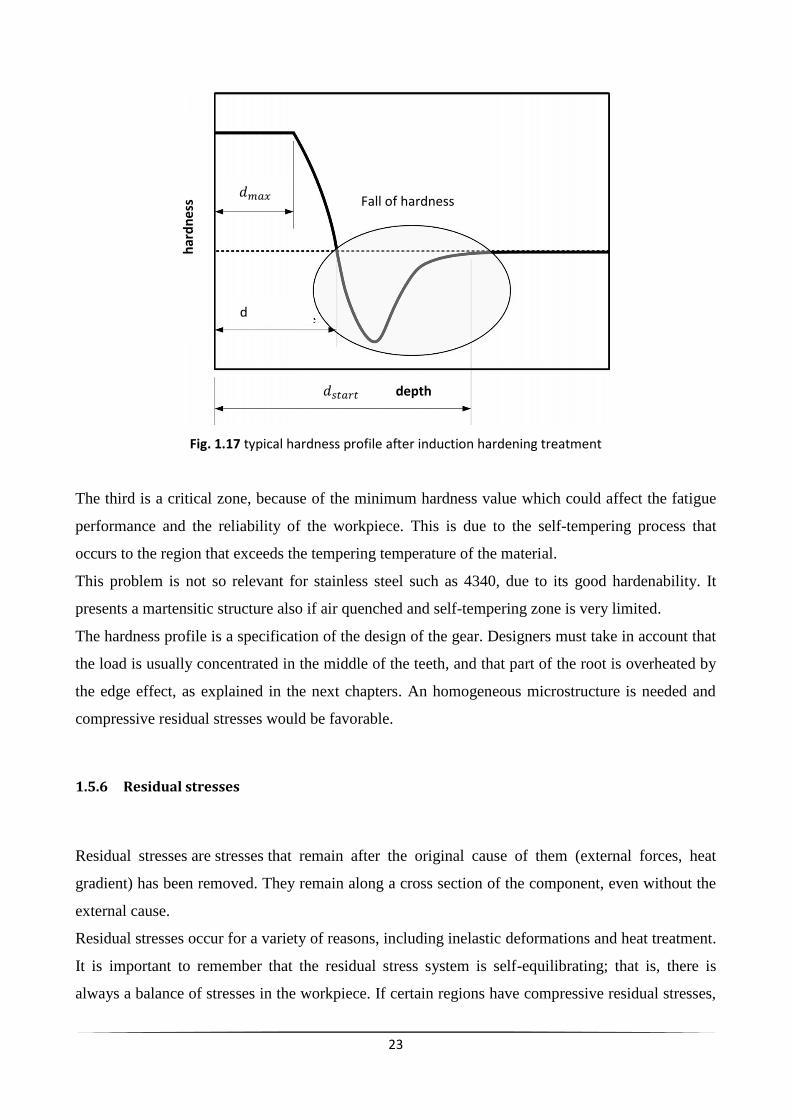
Nevertheless the typical hardness profile is formed by four distinct parts, as shown in figure 1.17.

The first is characterized by a maximum hardness, and the hardened depth is about 0.5 mm. In the

second zone hardness falls rapidly to a minimum, for then rising to the value of initial hardness in

the third part. The fourth and last part is not affected by the transformation during the metallurgical

treatment.

According to figure 1.17, we can distinguish these zones by three depths: maximum hardness depth

( ), the depth measured from the intersection between the curve and the initial hardness ( )

and finally, the depth of the area affected by the induction heat treatment (d).

23

Fig. 1.17 typical hardness profile after induction hardening treatment

The third is a critical zone, because of the minimum hardness value which could affect the fatigue

performance and the reliability of the workpiece. This is due to the self-tempering process that

occurs to the region that exceeds the tempering temperature of the material.

This problem is not so relevant for stainless steel such as 4340, due to its good hardenability. It

presents a martensitic structure also if air quenched and self-tempering zone is very limited.

The hardness profile is a specification of the design of the gear. Designers must take in account that

the load is usually concentrated in the middle of the teeth, and that part of the root is overheated by

the edge effect, as explained in the next chapters. An homogeneous microstructure is needed and

compressive residual stresses would be favorable.

1.5.6 Residual stresses

Residual stresses are stresses that remain after the original cause of them (external forces, heat

gradient) has been removed. They remain along a cross section of the component, even without the

external cause.

Residual stresses occur for a variety of reasons, including inelastic deformations and heat treatment.

It is important to remember that the residual stress system is self-equilibrating; that is, there is

always a balance of stresses in the workpiece. If certain regions have compressive residual stresses,

Fall of hardness

d

depth

har

dn

ess

24

then somewhere else there must be offsetting tensile stresses. If the stresses weren’t balanced,

“movement” would then result.

In general, two types of stress are encountered: thermal and phase transformation stresses.

Thermal stresses: Thermal stresses are caused by temperature gradients between the

surface and the core of the gear, due to the heating and cooling process. Considering the

cooling process, the surface cools faster than the heart, leading to a faster contraction. This

causes the surface to be tensioned, while the core becomes compressed. However, if

deformation is elastic-linear, the situation is temporary because when all the components

reach the same temperature deformation disappears.

Transformation stresses: Transformation stresses primarily occur due to volumetric

changes accompanying the formation of phases such as austenite, bainite, and martensite.

Considering the quenching phase of an induction hardening process, being the heat removed

from the surface, the martensitic transformation starts from the surface itself, while in depth

transformation needs more time to occur. Having austenite and martensite different specific

volumes, this causes the formation of stresses. These stresses will disappear once the

workpiece reaches a homogeneous temperature, if they don’t excess the threshold of elastic

deformations.

The total stress is a combination of the two components.

It often happens that stresses exceed the yield strength threshold, leading to inhomogeneous plastic

deformation within the piece. So residual stresses remain after the thermal equalization of the

workpiece.

It is important to remember that the phase variation leads also to a variation of the mechanical

properties, increasing the yield strength in the martensite.

It is possible to control the magnitude of residual stress by a careful study on the type and the

quenching speed. Compressive residual stresses on the surface layers, especially in the root of the

gear are desired. Indeed, they act as a prestress on the most strongly loaded surface layer, which

increases the load capacity of the machine part and prevents crack formation or propagation on the

surface. The machine parts treated in this way are suited for the most exacting thermomechanical

loads since their susceptibility to material fatigue is lower. Consequently, much longer operation

life of the parts can be expected.

Tensile residual stresses, on the other hand, can be dangerous. Having a maximum tensile stress

located just beneath the hardened case facilitates the subsurface crack initiation.

25

Fig. 1.18 Residual stresses for elasto-plastic material.

1.6 Power supplies for induction heat treatment

The complexity of induction hardening process is due to the large number of variables that

influence it. For example, to achieve a specific case hardening pattern of a gear, it is necessary

to have a device that provides the correct power/frequency/time combination. Depending on the

desired result, it is possible to use a large range of frequencies, as shown in figure 1.19.

Fig. 1.19 Range of frequency utilized in induction heating

26

Frequency is a very important parameter in the design of induction heating power supplies because

the power components must be rated for operation at the specified frequency. In particular, the

power circuit must guarantee that these components are operated with a proper margin to yield high

reliability at this frequency.

The coil geometry and the electrical properties of the material to be heated determine the coil

voltage, current and power factor. Defining these parameters is necessary to ensure that the output

of the power supply is capable of matching the requirements of the coil.

In general, an induction heating machine is composed of the power supply, the load matching and a

process control system, as shown in a basic diagram in figure 1.20.

Fig. 1.20 Induction heat treatment power supply, basic block diagram

1.6.1 Power supplies

Induction heating power supplies convert the available line frequency power to the desired single

phase power at the frequency required by the induction heating process.

Power supplies for induction hardening vary in power from a few kilowatts to hundreds of

kilowatts, and in frequencies from 1 kHz to 400 kHz, including dual frequency units, dependent of

the size of the component to be heated and the production method employed. Higher and lower

frequencies are available but typically these will be used for specialist applications.

In the early days of induction heating, the motor-generator, a rotary-driven system composed of a

motor coupled to a generator, was used extensively for the production of MF power up to 10 kHz,

until the advent of solid state technology in the early 1970s.

Initially, solid state power supplies was limited to the use of thyristors for generating the MF range

of frequencies using discrete electronic control systems. With this system, line voltage is converted

27

to direct current and then it is applied by means of a capacitive voltage divider to an SCR inverter

circuit.

State of the art units now employ IGBT or MOSFET technologies for generating current as of

MHz’s order of magnitude.

Fig. 1.21 switches utilized

A whole range of techniques are employed in the generation of MF and HF power using

semiconductors.

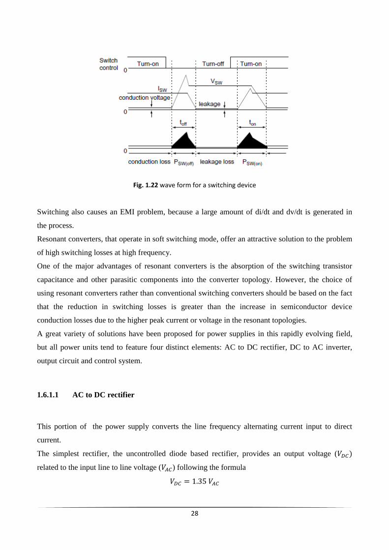
Semiconductor switching devices may operate in Hard Switch Mode in various types of PWM

(pulse width modulation) DC-DC converters and DC-AC inverter topology employed in a power

system. In this mode, a specific current is turned on or off at a specific level of voltage whenever

switching occurs. This process results in switching loss. The higher the frequency the more the

switching loss, which obstructs efforts to raise the frequency. Switching loss can be calculated with

the following formula:

Where is switching loss [W], is the switching voltage [V], is switching current [A],

switching frequency [Hz], is the switch turn-on time [s] and is the switch turn off time.

28

Fig. 1.22 wave form for a switching device

Switching also causes an EMI problem, because a large amount of di/dt and dv/dt is generated in

the process.

Resonant converters, that operate in soft switching mode, offer an attractive solution to the problem

of high switching losses at high frequency.

One of the major advantages of resonant converters is the absorption of the switching transistor

capacitance and other parasitic components into the converter topology. However, the choice of

using resonant converters rather than conventional switching converters should be based on the fact

that the reduction in switching losses is greater than the increase in semiconductor device

conduction losses due to the higher peak current or voltage in the resonant topologies.

A great variety of solutions have been proposed for power supplies in this rapidly evolving field,

but all power units tend to feature four distinct elements: AC to DC rectifier, DC to AC inverter,

output circuit and control system.

1.6.1.1 AC to DC rectifier

This portion of the power supply converts the line frequency alternating current input to direct

current.

The simplest rectifier, the uncontrolled diode based rectifier, provides an output voltage (

related to the input line to line voltage ( ) following the formula

29

Since no control of the output is carried out by this rectifier, it must be used with an inverter section

capable of regulating the power supply output.

The phase controlled rectifier has thyristor instead diode, that can be switched on in a manner that

provides control of the DC output relative to the input line voltage. However, the control response

time is slow and the input line power factor is not acceptable when the DC output voltage of the

converter is less than a minimum, so schemes with additional power components are required.

Another solution is to have an uncontrolled rectifier followed by a switch mode regulator (buck) as

shown in figure 1.23. This rectifier can therefore regulate the output power of the inverter by

controlling the supply of direct current.

Fig. 1.23 Uncontrolled rectifier with switch mode regulator

In most heat treatment situations where the power supply rating is less than 600 kW, and where

utility requirements do not require reduced harmonic content, a six pulse rectifier is acceptable. On

the other hand a 12 pulse rectifier or a H bridge rectifier can be used.

1.6.1.2 DC to AC inverter

The inverter portion converts the DC supply to a single phase AC output at the relevant frequency.

This features the SCR, IGBT or MOSFET and in most cases is configured as an H-bridge or an H-

half bridge.

Fig. 1.24 basic full-bridge inverter

30

The H-bridge has four legs each with a switch and the output circuit is connected across the centre

of the devices. When the relevant two switches are closed current flows through the load in one

direction. These switches then open and the opposing two switches close, allowing current to flow

in the opposite direction. By precisely timing the opening and closing of the switches, it is possible

to sustain oscillations in the load circuit.

The 2 major types of inverter most commonly used in induction heating power supplies are the

voltage-fed and the current-fed. Figure 1.25 shows the principal design features of the inverter

involved in induction heating.

Fig. 1.25 Induction heat treatment inverters

As shown in figure 1.25, the two principal types of inverter can be divided by the DC source (fixed

or variable), the mode of inverter control and the load circuit connection (series or parallel).

Voltage fed inverter with simple series load

Voltage fed inverters are distinguished by the use of a filter capacitor at the input of the

inverter and a series-connected output circuit as shown in the simplified power circuit

schematic of figure 1.26.

31

Fig. 1.26 Voltage-fed series-connected output

The series-loaded resonant converter topology has an important advantage over the parallel-

loaded resonant converter in high voltage applications since it does not require an output

inductor.

This inverter can be switched below resonance in the case of thyristor. Indeed diode

conduction must follow thyristor conduction for sufficient time to allow the tyristor to turn

off. Transistors do not require turn off time and therefore can be operated at resonance,

switching while current is zero, thus minimizing switching losses and maximizing power

transferred from the DC source to the load. To regulate power in this case the DC supply

voltage must be controlled. Transistors can also be switched above resonance and in this

case the conducting switches are turned off prior to the current reaching zero. This forces the

current to flow in the diodes that are across the non-conducting switches. The non-

conducting switches can then be turned on as soon as the load current change direction, thus

minimizing transistor and diode switching losses while allowing the inverter to operate off

resonance to regulate power.

In nearly all heat treatment applications, an output transformer is required to step up the

current available from the inverter to the higher level required by the induction heating coil.

Voltage fed inverter with series connection to a parallel load

This type of inverter has an internal series-connected inductor and capacitor that couple

power to a parallel resonant output as shown in figure 1.27.

32

Fig. 1.27 Voltage fed inverter with series connection to parallel load

An important characteristic of this kind of inverter is that the internal series circuit isolates

the bridge from the load, protecting the inverter from load faults caused for example by

shorting or arcing, or badly tuned loads. This feature make this inverter a very robust

induction power supply available for heat treatment.

The voltage fed inverter with series connection to a parallel load has an unregulated DC

input supply. Regulation of output power is done by varying the firing frequency relative to

the parallel load resonant frequency.

Current fed inverters

The current fed inverter uses a variable-voltage DC source followed by a large inductor at

the input of the inverter bridge and a parallel resonant load circuit at the output. Figure 1.28

shows a simplified power circuit of this inverter.

Fig. 1.28 Current fed full bridge inverter

Current fed inverter can be operated from the resonant frequency of the parallel resonant

load.

At the resonant frequency the switching or commutation is done when the voltage of the

load, inverter bus, and the switch is zero, minimizing the switching losses and therefore

33

allows for higher frequency operation. The output power musty be regulated by controlling

the input current to the inverter. This is accomplished by using a variable voltage DC

supply.

However power electronics is a rapidly evolving field, and several other inexpensive

inverter configurations have been proposed for heat treating.

In general voltage fed inverter is preferred in applications with high ohmic inductor like melting or

forging, due to its features. On the other hand current fed inverters are normally used for

applications with low ohmic inductor like hardening and tube welding.

1.6.2 Load matching

A very important task during the design of an induction heating machine is to successfully deliver

to the workpiece the maximum available power for a given power supply at the minimum cost.

In practice, it is usually best to tune the appropriate induction heating circuit to obtain a unity power

factor and then to match the coil and workpiece impedance to that of the power supply.

This involved variable ratio transformers, capacitors and sometimes inductors that are connected

between the output of the power supply and the induction coil and the adjustment of these

components is referred to as load matching. Indeed, the simple addition of an isolation transformer

is often not enough to satisfy the requirements of every component.

Moreover, since a relatively large current is required to successfully heat a workpiece, it is

necessary to build power sources with extremely high output current capability or to use a simple

resonant circuit to minimize the actual current or voltage requirement of the frequency converter

and in the same time relaxing also the requirement of interconnecting cables, contactors and

transformers operating in the area of the improved power factor.

It is not easy to get an optimal design of a complete induction heat treatment. Indeed the induction

coil quite often is designed to achieve the desired induction heat treatment pattern without regard to

the power supply that will be used. In this case, a flexible interface is required to match the output

characteristics of the power supply to the input characteristics of the induction coil and workpiece

combination.

Furthermore, material’s properties such as electrical conductivity and magnetic permeability vary

during the heating cycle. In addition, combinations of production mix and variation of materials

34

properties result in changing coil resistance and reactance, which affects the tuning and

performance of the power supply by changing the phase angle between the coil voltage and coil

current of a given circuit.

For example, flexibility is required if the heat treatment machine is general-purpose, such as a scan

hardening machine. In this case, the ability to match a wide range of coils at more than one

frequency is essential, and dual frequency capacitor banks is recommended.

1.6.3 Process control

The control section monitors all the parameters in the load circuit, providing an operator with

information about what is actually happening during the process and whether the heat treatment of

the workpiece has been successful.

With the advent of microcontroller technology, the majority of advanced systems now feature

digital control, allowing systems to measure many variables at once with corresponding real-time

graphing of the function within the preset set point as well as any required analysis.

For induction hardening, a list of possible variables that could ensure that the process has been

successfully repeated and what the correlation is between the variables and the heat treatment

process is shown in figure 1.29.

Fig. 1.29 variables in induction hardening

It highlights the fact that energy or coil monitors are not enough in a process as hardening, because

the quenching phase is as critical to the proper hardening of the part as the heating phase.

To make an example, variation in electrical resistivity and magnetic permeability during the heating

cycle leads to changes in penetration depth in the workpiece. This changes can be observed by

monitoring the coil voltage, current and phase angle at the induction coil. However in induction

hardening the actual change in inductance from cold to hot may be relatively small. Indeed, due to

35

the high power densities and magnetic field, relative magnetic permeability has relatively small

values, and since penetration depth varies as the inverse square root of , there will be not great

difference in inductance and impedance.

36

37

2. The gears and AISI 4340’s properties

2.1 Introduction

The material properties involved in an induction heating process were briefly described in chapter

1. They depend on the temperature and also on the microstructure and on some machine’s

parameters as the magnetic field and heating rate.

Usually, these properties are measured in thermodynamic equilibrium conditions but induction

hardening process is anything but in equilibrium. Indeed, as CHT diagrams show, heating rate may

affect phase transformation temperatures, in the heating phase and also in the cooling phase. This

affects also physical properties, by modifying the critical points. Usually, for high heating rate, they

are shifted, generally towards higher temperatures, as shown in chart 2.1. As a result, it is very

important to properly describe the materials properties in order to obtain a well-posed numerical

model.

The hardened spur gears that we considered are made of a quenched and tempered AISI 4340

martensitic steel.

Chart 2.1 Transformation’s temperature for AISI 4340 for different heating rate

Heating rate Ac1 [°C] Ac3 [°C] Acm [°C]

2739 °C/s 726 983 1058

814 °C/s 787 982 1048

427 °C/s 778 949 1038

99 °C/s 768 856 910

38

2.2 Test case 1

Fig. 2.1 Geometry of the gear of test case 1

The data that characterized the gear are summarized in chart 2.2.

Chart 2.2 Data of the gear

Pitch diameter [mm] 140

No. teeth 56

Module [mm] 2.5

Tooth thickness [mm] 3.656

Face width [mm] 9

2.3 Test case 2

Fig. 2.2 Geometry of the gear of test case 2

39

Chart 2.3 data of the gear

Number of teeth 48

Diametral pitch 12.00

Pressure angle 25.00°

Outside diameter 105.84 mm

Base diameter 92.08 mm

Root diameter 95.38 – 95.50 mm

Pitch diameter 101.6 mm

Form diameter 97.88 mm

Arc tooth thickness 3.20-3.25 mm

Tooth length 6.35 m

2.4 AISI 4340

AISI 4340 is a heat treatable, low alloy steel containing nickel, chromium and molybdenum. It is

very suitable for the process of induction hardening considered the carbon content and the alloying

elements which improve the hardenability and the mechanical properties of the heart. Indeed it is

known for its toughness and capability of developing high strength in the heat treated condition

while retaining good fatigue strength.

Typical applications are for structural use, such as aircraft landing gear, power transmission gears

and shafts and other structural parts.

Chemistry data of AISI 4340 are summarized below.

Chart 2.4 Chemistry data of AISI 4340

Element weight %

Carbon 0.38-0.43

Manganese 0.60-0.80

Phosphorus 0.035 (max)

Sulphur 0.04 (max)

Silicon 0.15-0.30

Chromium 0.70-0.90

Nickel 1.75-1.90

Molybdenum 0.20-0.30

40

2.4.1 Relative magnetic permeability

Magnetic permeability influences the skin depth, given by the following formula

and hence the power distribution due to the eddy currents.

The evolution of as a function of temperature is a simplistic representation of a much more

complex behavior. Indeed, neglecting the effect of the microstructure, the relative magnetic

permeability also depends on the magnetic field strength.

During high frequency induction heating, in itself very short, the different parts of the gear are

affected by different values of magnetic field. In the more complex cases of a preheating at medium

frequency or a double frequency, the variation in frequency influences also the distribution of the

magnetic field.

The measurement of remains a difficult task and requires advanced measurement techniques and

colossal resources for heating rates.

Figure 2.3 shows the behavior of as a function of temperature for different values of magnetic

field.

Fig. 2.3 (T) of steel for different magnetic field intensities

It is possible to see that all the curves have a common characteristic. Below Curie temperature, at

about 770°C, the permeability is decreasing while the magnetic field intensity is increasing. Above

the curie temperature, is always unity.

Temperature (°C)

Re

lati

ve m

agn

etic

per

me

abili

ty

41

In particular in literature it is shown that considering a higher initial value of the edge effect will

be enhanced and superficial temperatures of the workpiece increase, in a HF heating [9].

So, in the numerical model it is very important to consider the correct profile as a function of

temperature or, better, even as a function of magnetic field.

Furthermore, it is demonstrated by sensitivity study of material properties that relative magnetic

permeability is the parameter whose variations affect more the profile’s temperature, especially in

HF heating. This is due to its influence on skin effect and edge effect.

2.4.2 Specific heat

To quantify the effects of the heating rate on specific heat profile as a function of temperature for

AISI 4340, three curves Cp1, Cp2 and Cp3 are considered in figure 2.4.

Fig. 2.4 different specific heat curves for AISI 4340, as a function of temperature

These curves are obtained by shifting temperatures Ac1 and Ac3 and assuming constant the latent

heat peak, taking into account the variations of critical points of steel due to high heating rate.

This behavior generally allows the workpiece to reach lower maximum temperature, due to the

higher energy required for heating a material which has higher specific heat (area of the shifted

curve is greater that the non shifted curves).

Temperature °C

Spe

cifi

c h

eat

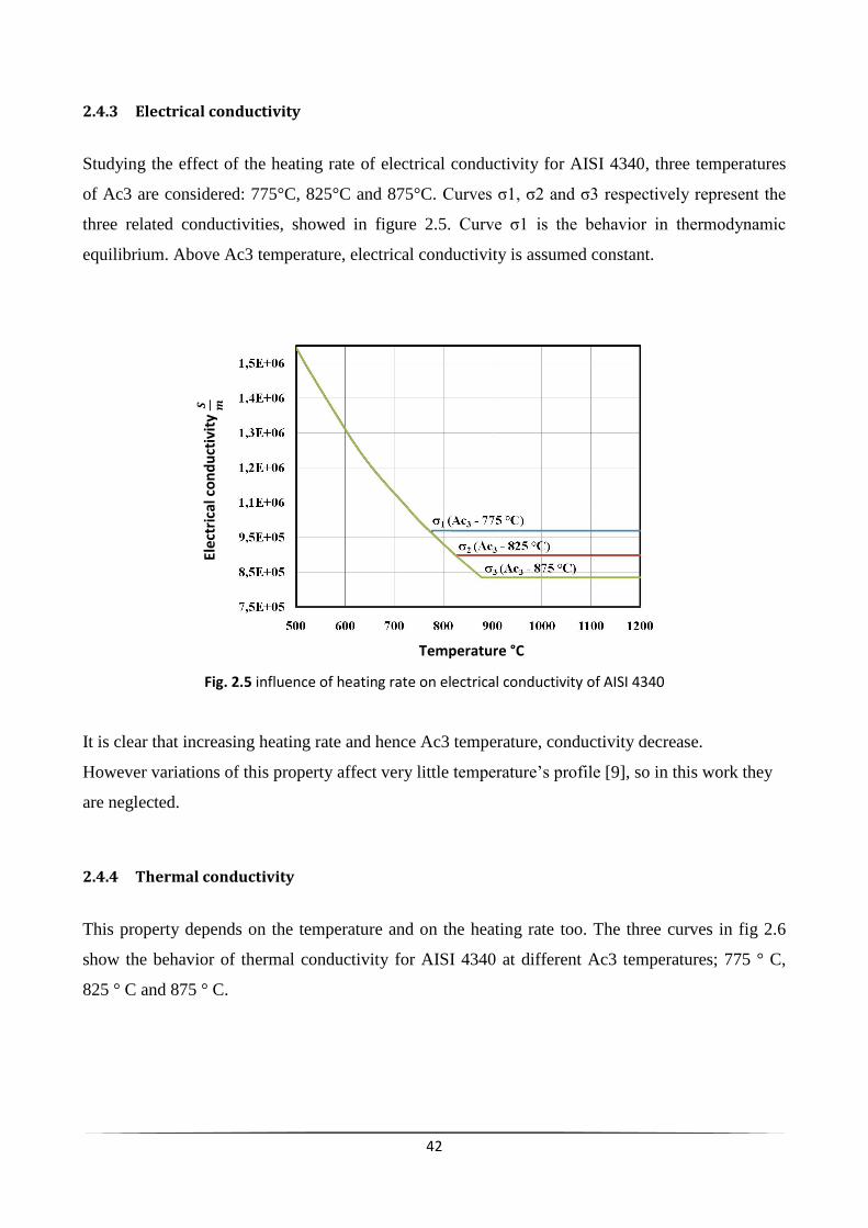
42

2.4.3 Electrical conductivity

Studying the effect of the heating rate of electrical conductivity for AISI 4340, three temperatures

of Ac3 are considered: 775°C, 825°C and 875°C. Curves σ1, σ2 and σ3 respectively represent the

three related conductivities, showed in figure 2.5. Curve σ1 is the behavior in thermodynamic

equilibrium. Above Ac3 temperature, electrical conductivity is assumed constant.

Fig. 2.5 influence of heating rate on electrical conductivity of AISI 4340

It is clear that increasing heating rate and hence Ac3 temperature, conductivity decrease.

However variations of this property affect very little temperature’s profile [9], so in this work they

are neglected.

2.4.4 Thermal conductivity

This property depends on the temperature and on the heating rate too. The three curves in fig 2.6

show the behavior of thermal conductivity for AISI 4340 at different Ac3 temperatures; 775 ° C,

825 ° C and 875 ° C.

Temperature °C

Ele

ctri

cal c

on

du

ctiv

ity

43

Fig. 2.6 Thermal conductivity for different Ac3 temperatures

The curves show that thermal conductivity reaches a minimum at the austenitization temperature.

However, even in this case, variations of this property don’t affect much the surface’s temperatures

[9], so we will neglect them on numerical model.

Temperature °C

Ther

mal

co

nd

uct

ivit

y

44

45

3. Numerical modeling of the process

3.1 Introduction

The design of induction hardening devices and the choice of the hardening parameters such as

frequency, inductor’s current and power, are often carried out by experience and experimentation.

Nevertheless, as mentioned before, this approach results very expensive and difficult if complex

geometries of the workpiece are involved and even studying the effect of the variation of hardening

parameters results very hard. Thus, simulations dramatically reduce development time of the

process and reduce rejection of samples.

The numerical simulations of induction heating process offer new possibilities in these fields.

Together with validation tests, these models provide an essential solution to control the method of

heat treatment by induction.

The finite element method (FEM) is a numerical technique for obtaining an approximate solution to

different technical problems, including those encountered in induction heat treatment.

In general in finite element discretization we have that the area of study is subdivided into

nonoverlapping finite elements. The sides of finite elements intersect at nodes.

The FEM provides an element wise approximation to the governing equations (reported below),

solving the global set of resulting simultaneous algebraic equations with respect to the unknown, for

example magnetic vector potential at each node in the region of evaluation.

46

To obtain reasonable accuracy of the numerical solution, the finite element mesh has to be relatively

fine in the regions where the rate of change of the unknown (i.e. magnetic vector potential and

temperature) is high.

The current density, flux density, conductivity, magnetic permeability and other material properties

are postulated to be constant within each element.

In order to reduce the complexity of the computation, the designer should take advantage of the

symmetry involved in the system geometry.

After solving the system of algebraic equations and obtaining the distribution of the magnetic vector

potential in the region of modeling, it is possible to find all the required output parameters of the

electromagnetic field such as:

- induced current density in conductors

- total current density in the conductor

- magnetic flux density components by the relation and hence flux density

- magnetic field density from the relation

- electric field intensity

- Electromagnetic force density in current-carrying conductors and in the workpiece by

the formula

Finally from a vector potential solution it is possible to compute the other important quantities of

the process such as energy stored, flux leakage, total power loss and coil impedance.

Different finite element programs are used for the computation of coupled electromagnetic and

thermal problems, such as ANSYS, COMSOL and FLUX. These tools also allow to take into

account important temperature-dependent material parameters. FLUX 3D is used in this study to

carry out different analysis.

In this chapter the steps needed to build simulations and related problems have been described,:

Building of the geometry

Building of the mesh

Description of the materials and their properties

Description of the problem and of the boundary conditions

Post-processing and analysis of the results

47

3.2 Building of the geometry

FLUX 3D allows designers to import geometries drawn with CAD-CAE software. Simple

geometries could be drawn directly on FLUX. The geometry of test case 1 has been imported from

CAD-CAE software. This gear is showed in the picture of this chapter. The geometry of test case 2

has been designed directly on FLUX.

In order to reduce the computing time, it is necessary to reduce as much as possible the geometry,

by exploiting the symmetries of the workpiece.

In the case of a gear, the original circular geometry is reduced in a quarter of tooth exploiting the

tooth periodicity and its symmetry along the middle radial plane.

Fig. 3.1 Geometry and infinite box, test case 1

The coil has been designed only taking into account the active part and considering only the

electrical properties. This hypothesis is not so far from reality because the coil is water cooled, and

its temperature doesn’t change a lot during the process. Moreover, at high frequency, current will be

distributed mainly on the interior surface of the coil, due to the skin effect and the proximity effect.

48

At the boundary of the simulation domain, infinite boundary conditions have been posed in order to

let the magnetic field vanish at infinite distance by means of an “infinite Box”.

The effect of a ring made in magnetic but non-conductive material above the gear, called flux

concentrator, has also been studied in the analysis of the model. All the parts of the model (the gear,

the coil, the flux concentrator and the infinite box) were split into different volumes, in order to

allow the designer to better develop the mesh and the model in general.

3.3 Building of the mesh

As mentioned before, when defining the mesh it is very important that superficial elements are very

dense. It is also very important to accurately describe the surface of the inductor because its current

will be distributed in a thin layer, due to skin effect, ring effect and proximity effect.

The conditions are more critical at higher frequency, where is lower. In this work the maximum

frequency considered was 250 kHz, so we have

Where we consider for copper that

And for AISI 4340 we have

Hence it is necessary to have at least 2 surface elements of about 0.05 mm to obtain truthfully

results and for the convergence of the solution.

49

Moreover, as shown in figure 3.2, a superficial volume has been built in the coil and in the gear that

have mapped mesh, rather that automatic such as in the other parts of the model.

Fig. 3.2 mapped mesh on the coil and on the inductor, test case 1

In the inner areas of the gear, where magnetic field is weaker than in the surface, a more relaxed

mesh has been designed, reducing the number of elements and hence the computation time.

Likewise, in the interior part of the coil a relaxed mesh has been built.

Differentiation of the dimensions of mesh elements was possible by creating what is called “mesh

lines”. Indeed, we imposed the length of the elements at the beginning and at the end of lines,

relaxing the mesh when low magnetic field is involved.

Fig. 3.3 example of mesh lines.

50

3.4 Description of materials and their properties

As already clarified, we have to introduce some approximations for the description of the model,

due to the uncertainty of data in literature and to the limits of the simulation programs.

1. Gear: The properties of AISI 4340 have been described in the previous chapter. In

particular it is not easy to solve complex computational models with relative permeability

function of both temperature and magnetic field. An alternative could be using a magnetic

permeability function only of temperature, taking in account the magnetic field agent

choosing the value of (see figure 3.4).

Fig. 3.4 relative magnetic permeability as a function of temperature, test case 1

Volumetric heat capacity trend for test case 1 is shown in figure 3.5.

Fig. 3.5 Volumetric heat capacity, test case 1

0

2

4

6

8

10

12

0 500 1000 1500 2000

Re

lati

ve M

agn

eti

c P

erm

eab

ility

Temperature [°C]

Relative Magnetic Permeability

0

2000000

4000000

6000000

8000000

10000000

12000000

14000000

0 200 400 600 800 1000 1200 1400 1600

Vo

lum

etr

ic H

eat

Cap

acty

[J/

m^3

*°C

]

Temperature [°C]

Volumetric Heat Capacity

51

The superficial average heating rate was taken into consideration by shifting the specific

heat peak. For the computation of heating rate in the different recipes we considered only

the HF heating.

Chart 3.1 Heating rate

HF heating (s) Ac1 (°C) Ac3 (°C) Average superficial

Heating rate (°C/s)

Test case 1 0.2 778 949 2700

Test case 2 2 726 983 500

Electrical and thermal conductivity are shown in figure 3.6 and 3.7 respectively.

Fig. 3.6 electrical conductivity as a function on temperature, test case 1 and 2

Fig. 3.7 thermal conductivity as a function of temperature, test case 1 and 2

0.00E+00

1.00E+06

2.00E+06

3.00E+06

4.00E+06

5.00E+06

0 200 400 600 800 1000 1200 1400 1600

Co

nd

uct

ivit

y [S

/m]

Temperature [°C]

Conductivity

0

5

10

15

20

25

30

35

40

45

0 200 400 600 800 1000 1200 1400 1600

The

rmal

Co

nd

uct

ivit

y [J

*m^

-1*s

^1*

°C^

-1]

Temperature [°C]

Thermal Conductivity

52

We neglect the influence of high heating rate on the latter two properties.

2. Coil: The coil is made of copper. We consider the resistivity .

3. Flux concentrator: Soft magnetic composites materials iron-and-ferrite-based compositions

called flux concentrators are provided by different industries in order to obtain selective

heating of certain areas of the workpiece, improving the electrical efficiency of the induction

coil and acting as an electromagnetic shield to prevent the undesirable heating of adjacent

regions. As a result these materials must have a high relative permeability and low-power-

losses.

One of the flux concentrator used in induction heating is “FLUXTROL 50”, because of its

good performance over a wide range of frequencies (10-1000 kHz).

Chart 3.2 Properties of FLUXTROL 50

Density 6.1 g/cm3 Initial Permeability 36

Maximum Permeability 55 Saturation Flux Density 1.5 T

Operating Frequency Range 10-1000 kHz Major Frequency Range 50-500 kHz Temperature Resistance 250 °C Long Term

300 °C Short Term Thermal Conductivity 0.06 W/cm K

Resistivity 0.5

In numerical models simplifications are necessary in order for the model to be solved in a

reasonable time. In particular, considering the value of magnetic field involved in the

induction hardening process, we assume for the flux concentrator a value of relative

magnetic permeability of 40, constant with temperature. Moreover, the actual resistivity of

FLUXTROL 50 is very high and so we can assume that it is non conductive. These

assumption allows the model to be simplified without making too many mistakes.

3.5 Description of the problem and of the boundary conditions

Solving the coupled magnetic and thermal problem to simulate the induction hardening process, the

“Steady-state AC Magnetic Transient Thermal” has been chosen.

53

To complete the model, it has been necessary to define “volume regions”, and assign them to “real”

volumes, in order to assign the behavior of the different part of the model. The volume regions

created could be described as follows.

Chart 3.3 Volume regions

VOLUME REGION MAGNETIC

DEFINITION

THERMAL

DEFINITION

MATERIAL

AIR Air or Vacuum region Inactive region /

COIL Solid conductor region Inactive region Copper

GEAR Solid conductor region Heat computed by Joule

effect

AISI 4340

FLUX

CONCENTRATOR

Magnetic non

conducting region

Inactive region Fluxtrol 50

Moreover, a voltage control has been chosen to regulate the power in the workpiece. This was done

by imposing an electric potential at the end of the inductor. Taking into account the symmetries of

the problem the electric potential has been assigned to the faces of a fraction of the entire circular

section of the inductor. This was done by creating two “face regions”, described in chart 3.4.

Another face region was created to play back the effect of losses by radiation and convection. For

convection an α coefficient of 10 has been considered while for radiation losses a value of

has been chosen. These conditions have been assigned in the external part of the gear that are the

hottest.

Fig. 3.8 external faces subject to radiation and convection losses, test case 1

54

chart 3.4 Face regions

REGION MAGNETIC DEFINITION THERMAL DEFINITION

V0 Boundary condition: Imposed

electrical potential

Inactive region

V1 Boundary condition: Imposed

electrical potential

Inactive region

EXCHANGE Inactive Region Surface of thermal exchange and

heat source

3.6 Computation and post processing of the results

Once the mesh and the physics of the problem have been designed, the model is ready for the

computation.

For the computation it is important to remember for the computation that:

Very short time steps are required during high power variations, such as at the beginning or

at the end of a heating phase, to allow the convergence of the method.

Longer time step are required during the preheating phase in MF, as there are lower values

of temperature and power density gradient in the workpiece.

Short time steps are required for the convergence of the method in the heating phase in HF,

due to the higher temperature and power density gradient.

Simulations have been solved with a Professional Workstation, and computing time varied from

three to six hours, as a function of the number of time steps implemented.

It has been possible to achieve a great number of output parameters in all the time steps, as already

clarified.

55

56

4. Optimization of induction hardening parameters

4.1 Introduction

In this work simulations are used to study the effect of machine’s parameters such as frequency and

dimension of the inductor on the distribution of temperature, and also to evaluate the effect of a flux

concentrator above the gear. This in order to obtain a homogeneous hardened profile of at least 0.6

mm, both in the tip and in the tooth of the gear. Furthermore is also important to prevent the entire

tooth from being austenitised, avoiding unwanted phenomena which would lead to a deterioration

of the mechanical properties.

Numerical models are very useful for this kind of study. Indeed, they allow researchers to save a

great amount of energy, materials, time and equipment needed for the measurements. Moreover it is

possible to compute the parameters, such as power, needed by designers in order to design properly

an induction hardening machine.

Once the model of test case 1 has been built following the principle explained in the previous

chapter, the induction hardening process was split into 3 periods. The first, preheating at MF; the

second, an interruption of power of 0.2 s needed by experimental devices for changing the

frequency and required also by diffusion to homogenize the temperature; finally, the third, the real

hardening that consists in 0.2 s HF at 350 kW.

4.2 Influence of flux concentrator

To understand the effect of the flux concentrator, 3 models have been created: Recipe A and B with

two different thicknesses of flux concentrator (2 and 1 mm respectively) and recipe C without it. All

the simulation consists in a 3 s of preheating phase at 5000 Hz, and 0.2 s of heating phase at 200

kHz. The dimension of the inductor is 8 mm height and 8 mm thick.

The following figures show the inducted power density, the magnetic field arrows and the

temperature’s profile at the end of the HF heating phase for all the recipes.

57

Fig. 4.1 900°C isotherm at the end of HF heating, recipe A

Fig. 4.2 magnetic field arrows at the end of HF heating, recipe A

Fig. 4.3 power density at the end of HF heating, recipe A

58

Fig. 4.4 900°C isotherm at the end of HF heating, recipe B

Fig. 4.5 magnetic field arrows at the end of HF heating, recipe B

Fig. 4.6 power density at the end of HF heating, recipe B

59

Fig. 4.7 900°C isotherm at the end of HF heating, recipe C

Fig. 4.8 magnetic field arrows at the end of HF heating, recipe C

Fig. 4.9 power density at the end of HF heating, recipe C

60

It is possible to see how magnetic field lines tend to close in the workpiece, causing the edge effect.

This phenomenon is more marked in the model without flux concentrator, both in the tip and in the

root. As a result, the maximum power density value is about twice in the case without flux

concentrator in the external part of the root. In order to evaluate the uniformity of the heating

between the middle and the surface of the gear, the parameter of uniform heating is introduced as

Where SM is the heating depth in the surface of the gear, and MD in the middle. The more P.U.H.

is close to unity, the more the heating is homogeneous.

Chart 4.1 Depth of the 900°C isotherm

Root tip

Recipe Thickness of the flux concentrator (mm)

MD (mm) SM (mm) P.U.H MD (mm) SM (mm) P.U.H.

A 2 0.58 0.66 0.88 1.69 1.63 1.04

B 1 0.59 0.71 0.83 1.68 1.53 1.10

C / 0.66 1.33 0.50 1.06 1.61 0.66

Consequently, the flux concentrator allows the workpiece to obtain a more homogeneous power

density throughout the length of the root, and hence a better distribution of temperature between the

external part and the internal part of the gear. This will certainly evolve in a more homogeneous

hardened layer. We can conclude that the higher thickness the flux concentrator has, the smaller is

the edge effect, at the same power applied. However increasing the thickness of the flux

concentrator beyond 1 mm doesn’t reduce much more the edge effect.

4.3 Influence of inductor’s dimensions

Three simulations with different height of the coil are proposed. A 1 mm thickness flux

concentrator has been left. A 3 s, 5 kHz preheating and a 0.2 s, 200 kHz shot have been proposed

for all the recipes. For the simulations to be comparable, the same current was flowing in the

inductor.

Recipe height of the coil (mm)

D 6

E 8

F 10

61

Fig. 4.10 900°C isotherm at the end of HF heating, recipe D

Fig. 4.11 900°C isotherm at the end of HF heating, recipe E

Fig. 4.12 900°C isotherm at the end of HF heating, recipe F

62

Figures show that the dimension of the coil affects the final distribution of temperature. In particular

if the height of the coil is rather small compared with the height of the gear, the external part of the

tip remains colder than the core of the tip. This behavior is certainly caused by the fact that the eddy

current in the gear are mainly distributed in the section in front of the coil. On the other hand, if the

coil’s height is greater than the height of the gear, the external part of the tip are more heated. It is

important to remember that in the edge of the gear the power density are higher because of the edge

effect. Therefore the choice of the dimension of the coil is a compromise in order to obtain a

heating as homogeneous as possible along the contour of the tooth. Usually a coil slightly lower

than the gear is chosen.

4.4 Influence of the frequency and the duration on MF preheating phase

In order to understand how preheating phase affects the final distribution of temperature, different

models have been proposed. The same 200 kHz, 0.2 s heating phase is considered for better

comparison.

Recipe Preheating time (s) Preheating frequency (kHz)

1 1 10000

2 1 5000

3 1 1000

4 3 10000

5 3 5000

6 3 1000

7 5 10000

8 5 5000

9 5 1000

The power of the different preheating phase was calibrated by varying the tension of the inductor so

as to achieve the same superficial temperature at the end of the MF heating, always kept below

600°C in order to avoid modifications of the microstructure.

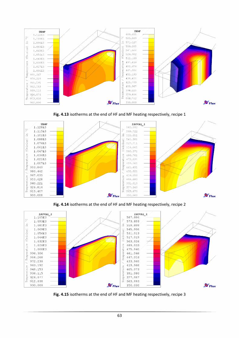
63

Fig. 4.13 isotherms at the end of HF and MF heating respectively, recipe 1

Fig. 4.14 isotherms at the end of HF and MF heating respectively, recipe 2

Fig. 4.15 isotherms at the end of HF and MF heating respectively, recipe 3

64

Fig. 4.16 isotherms at the end of HF and MF heating respectively, recipe 4

Fig. 4.17 isotherms at the end of HF and MF heating respectively, recipe 5

Fig. 4.18 isotherms at the end of HF and MF heating respectively, recipe 6

65

Fig. 4.19 isotherms at the end of HF and MF heating respectively, recipe 7

Fig. 4.20 isotherms at the end of HF and MF heating respectively, recipe 8

Fig. 4.21 isotherms at the end of HF and MF heating respectively, recipe 9

66

The chart presented below shows for the nine recipes the depth of the 900°C isotherm in the root

and in the tip at the end of HF phase.

Chart 4.2 Depth of the 900°C isotherm

Recipe 900°C depth in the tip 900°C depth in the root

SM (mm) MD (mm) SM (mm) MD (mm)

1 0.63 1.15 0.66 0.52

2 1.35 1.57 0.65 0.52

3 1.10 1.35 0.56 0.44

4 1.18 1.48 0.77 0.65

5 1.54 1.69 0.71 0.58

6 1.4 1.59 0.62 0.51

7 1.38 1.57 0.81 0.69

8 1.50 1.65 0.72 0.59

9 1.45 1.62 0.65 0.54

From a first graphical interpretation we can see that at 10000 Hz the longer preheating is, the higher

is the temperature in the root at the end of the MF phase. This is certainly due to the fact that the

penetration depth at 10000 Hz in the AISI 4340 steel is rather small (0.8 mm), and the induced

power is deposited superficially. Therefore heat flows from the tooth towards the root and having

longer preheating phase allows the root to be more heated.

Indeed, the more difficult task in induction hardening is to heat the root, from where the heat will

flow towards the core of the gear by conduction, despite the fact that inducted power is

concentrated in the root. So a preheating that allows the root to reach a higher temperature leads to a

more homogeneous hardened profile.

A different behavior is noticed for 1000 Hz preheating. Indeed figures show that the more

preheating lasts, the more the heat flows from the root to the other parts of the gear. This is due to

the higher penetration depth, that allows to heat directly the root, and longer preheating makes the

heat flow in other parts of the gear.

In the 5000 Hz preheating the behavior is between the other two cases.

There are not so many differences between the distribution of temperature of the 9 recipes after HF

heating. Nevertheless, we can conclude that a long 1000 Hz preheating would be better in order to

obtain an hardened depth in the tooth close to the one in the root, compatibly with the characteristic

of the power generator.

67

4.5 conclusions

It is possible to summarize the obtained results as follows:

The presence of the flux concentrator over the gear is very important to reduce the edge

effect, otherwise difficult to control.

In both cases of 5 and 10 kHz MF phase, longer preheating (5 s) allows the root to be better

heated than shorter preheating.

Preheating phase with lower frequency (1 kHz rather that 10 kHz) leads to better profile

temperature’s at the end of HF phase, because the root is better preheated. In this case,

longer preheating phase allows the heat to flow also toward the parts adjacent to the root.

Variations on the dimension of the coil affect the final temperature’s distribution. In order to

the power to be equally distributed, the height of the coil should not be greater than the

height of the gear.

68

69

5. Validation of numerical modeling

5.1 Introduction

Due to the complexity of the phenomena involved in the process of induction hardening, it is

necessary to introduce several simplifications and approximations in the numerical model, such as

in the description of relative magnetic permeability as a function of temperature and magnetic field

strength. These simplifications may lead to errors in the distributions of temperature and hence also

in the final microstructure of the material of the workpiece.

In this chapter we are going to compare the experimental results of an induction hardening process

of a gear with those obtained from simulations, in order to validate the numerical models, and

investigate the possibility to use them for the prediction of hardness profile.

5.2 Analysis of experimental procedure

A robust method is used for the measurement of surface temperature fields during fast induction

heating.

It is based on the original coupling of temperature indicating lacquers and a high-speed camera

system. Image analysis tools have been implemented to automatically extract the temporal

evolution of isotherms.

This method allows the full history of surface isotherms to be accurately documented for a 2 s high

frequency heating.

Prior to each test, the upper side of the spur gear was coated with a specific temperature indicating

lacquer. Such lacquers contain chemicals in suspension that transform or evaporate at given

temperatures, with an accuracy of ± 1% of the indicated temperature. A high-speed camera is set 25

cm above the gear by means of a tripod. The magnification is adjusted so that two teeth are

observed within the camera's field of view. The gear is lightened up enough for the lacquer coating

to appear uniform.

70

The camera records 512*352 pixels images at a frame rate of 2000 images per second. A typical

image is shown in figure 5.1.

.

Fig. 5.1 Typical Image of the acquisition.

The induction heating treatments were performed using a single turn coil on a dual simultaneous

MF and HF frequencies generator designed by EFD Induction. The coil has a 110-mm inner

diameter and a 8-mm thickness.

Fig. 5.2 Experimental setting.

71

A final air cooling without rotating the gear is expected.

A full characterization of the temperature evolution versus time has been conducted at the surface

of 2 teeth of the gear heated by 2 s HF heating at 45 kW and then cooled in air.

Two isotherms, 816⁰C, and 927⁰C, were acquired every 0.3 ms with a spatial resolution of 0.045

mm per pixel.

5.3 Numerical simulation

A steady-state AC Magnetic 3D with Thermal Transient model of the gear has been built in FLUX

3D, following the method proposed in chapter three.

Fig. 5.3 Model of the gear in FLUX 3D

It has been chosen to build a mapped mesh 0.5 mm depth on the tooth profile and in the external

part of the inductor, due to the value of skin depth at 190000 Hz

Fig. 5.4 mesh used in the model

72

Four different simulations have been considered, in order to understand the influence of the

material’s properties on the temperature distribution:

Recipe 1: A value of has been considered. The variation of the relative magnetic

permeability is shown in figure 5.5.

Fig. 5.5 Relative magnetic permeability trend in recipe 1

The trend of specific heat as a function of temperature is the one you can find in literature,

and it does not take into account the variation of the temperature Ac1 and Ac3 as a function

of the heating rate.

Fig. 5.6 Volumetric heat capacity trend in recipe 1

Recipe 2: The second simulation has been done by keeping the same volumetric heat

capacity trend of the first simulation, and considering the , according with figure

5.7.

0

2

4

6

8

10

12

0 500 1000 1500 2000

Re

lati

ve M

agn

eti

c P

erm

eab

ility

Temperature [°C]

Relative Magnetic Permeability

0

2000000

4000000

6000000

8000000

10000000

12000000

14000000

0 200 400 600 800 1000 1200 1400 1600

Vo

lum

etr

ic H

eat

Cap

acty

[J/

m^3

*°C

]

Temperature [°C]

Volumetric Heat Capacity

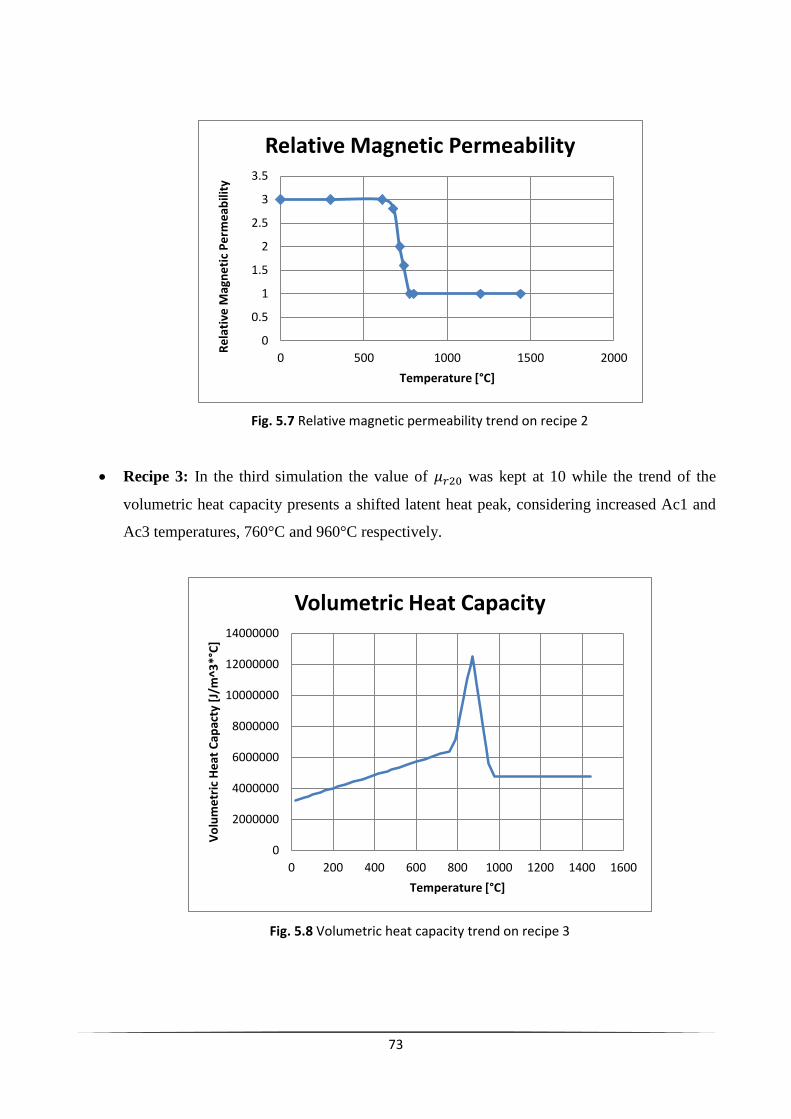
73

Fig. 5.7 Relative magnetic permeability trend on recipe 2

Recipe 3: In the third simulation the value of was kept at 10 while the trend of the

volumetric heat capacity presents a shifted latent heat peak, considering increased Ac1 and

Ac3 temperatures, 760°C and 960°C respectively.

Fig. 5.8 Volumetric heat capacity trend on recipe 3

0

0.5

1

1.5

2

2.5

3

3.5

0 500 1000 1500 2000

Re

lati

ve M

agn

eti

c P

erm

eab

ility

Temperature [°C]

Relative Magnetic Permeability

0

2000000

4000000

6000000

8000000

10000000

12000000

14000000

0 200 400 600 800 1000 1200 1400 1600

Vo

lum

etr

ic H

eat

Cap

acty

[J/

m^3

*°C

]

Temperature [°C]

Volumetric Heat Capacity

74

Recipe 4: In this recipe the value of was kept equal to 3 and the latent heat peak was

shifted as in recipe 3.

5.4 Comparison between experimental and numerical result: Isotherm’s

evolution

The first step in the validation of numerical models was the analysis of the isotherm’s evolution.

The simplest recipe of induction hardening has been considered (2 s HF), i.e. without preheating or

double frequency hardening in order to avoid the influence of other parameters. Indeed no lower

temperature lacquers have been used in the experimental procedure.

In the development of the numerical models, the power has been calibrated by considering the 816 °

C’s isotherm depth in the root of the gear equal to the experimental one at the end of the 2 s HF.

Here images of the gear are shown at different time steps of the heating phase, for each of the four

recipes.

75

T=2 s

Fig. 5.9 sights of experimental isotherms Fig. 5.10 simulated isotherms,

Fig. 5.11 simulated isotherms, Fig. 5.12 simulated isotherms, , shifted latent heat peak

Fig. 5.13 simulated isotherms, , shifted latent heat peak

76

T=1.92 s

Fig. 5.14 sights of experimental isotherms Fig. 5.15 simulated isotherms,

Fig. 5.16 simulated isotherms, Fig. 5.17 simulated isotherms, , shifted latent heat peak

Fig. 5.18 simulated isotherms, , shifted latent heat peak

77

T=1.86 s

Fig. 5.19 sights of experimental isotherms Fig. 5.20 simulated isotherms,

Fig. 5.21 simulated isotherms, Fig. 5.22 simulated isotherms, , shifted latent heat peak

Fig. 5.23 simulated isotherms, , shifted latent heat peak

78

T=1.80 s

Fig. 5.24 sights of experimental isotherms Fig. 5.25 simulated isotherms,

Fig. 5.26 simulated isotherms, Fig. 5.27 simulated isotherms, , shifted latent heat peak

Fig. 5.28 simulated isotherms, , shifted latent heat peak

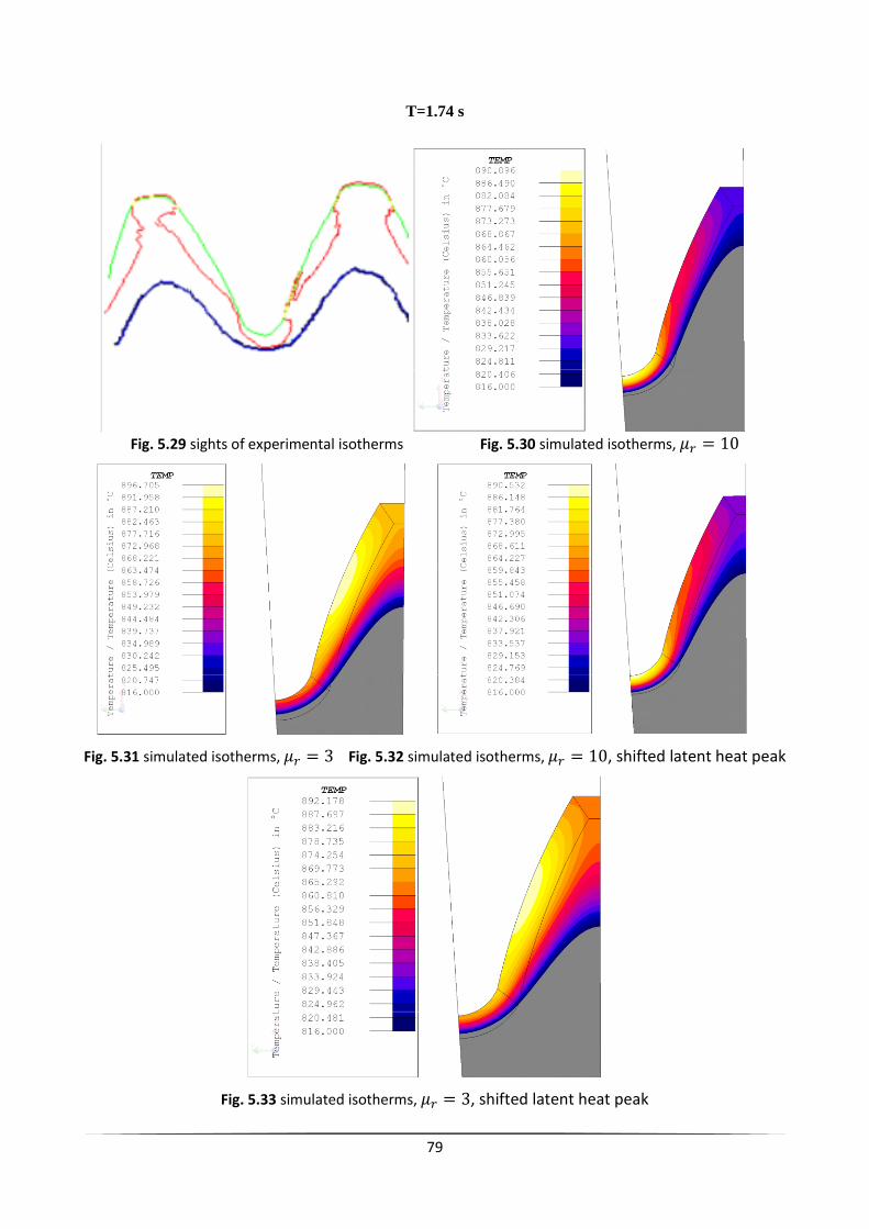
79

T=1.74 s

Fig. 5.29 sights of experimental isotherms Fig. 5.30 simulated isotherms,

Fig. 5.31 simulated isotherms, Fig. 5.32 simulated isotherms, , shifted latent heat peak

Fig. 5.33 simulated isotherms, , shifted latent heat peak

80

T=1.70 s

Fig. 5.34 sights of experimental isotherms Fig. 5.35 simulated isotherms,

Fig. 5.36 simulated isotherms, Fig. 5.37 simulated isotherms, , shifted latent heat peak

Fig. 5.38 simulated isotherms, , shifted latent heat peak

81

T=1.60 s

Fig. 5.39 sights of experimental isotherms Fig. 5.40 simulated isotherms,

Fig. 5.41 simulated isotherms, Fig. 5.42 simulated isotherms, , shifted latent heat peak

Fig. 5.43 simulated isotherms, , shifted latent heat peak

82

T=1.50 s

Fig. 5.44 sights of experimental isotherms Fig. 5.45 simulated isotherms,

Fig. 5.46 simulated isotherms, Fig. 5.47 simulated isotherms, , shifted latent heat peak

Fig. 5.48 simulated isotherms, , shifted latent heat peak

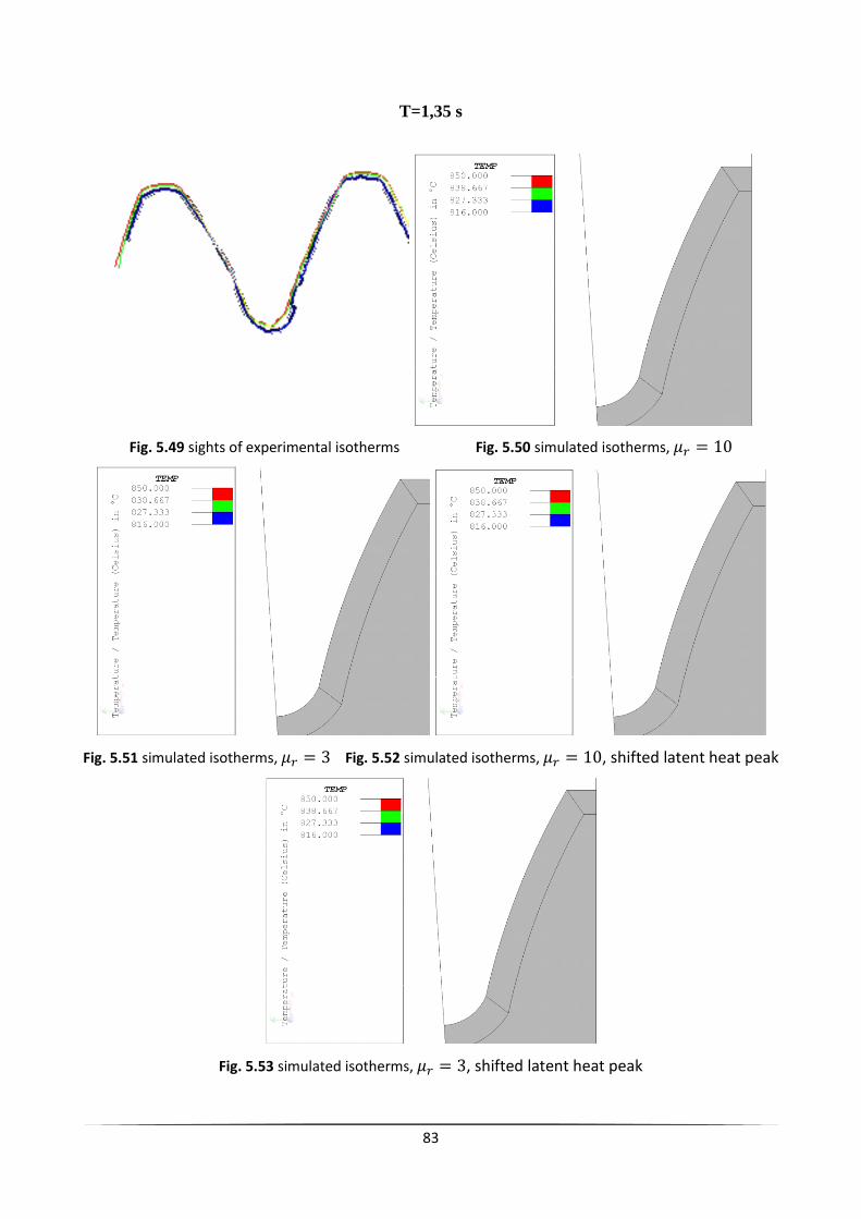
83

T=1,35 s

Fig. 5.49 sights of experimental isotherms Fig. 5.50 simulated isotherms,

Fig. 5.51 simulated isotherms, Fig. 5.52 simulated isotherms, , shifted latent heat peak

Fig. 5.53 simulated isotherms, , shifted latent heat peak

84

After the first graphical evaluation it is important to consider the actual depth of the two isotherms

considered. For this reason the isotherm’s depth has been reported in the following graphs for the

different time steps, for all the three recipes.

Fig. 5.54 depth of the 816°C and 927°C isotherms on the root of the gear.

Fig. 5.55 depth of the 816°C and 927°C isotherms on the tip of the gear

Observations

A qualitative analysis of the evolution of the experimental isotherms highlights the fact that the

temperature rises first at the root (fig. 5.39). Then, there is another starting point of the same

isotherm in the flank of the tooth (fig. 5.34) and subsequently it continues growing until reaching

the isotherm on the other flank of the tooth.

Consequently, despite the fact that HF heating is known to heat the nearest parts of the tooth to the

coil, i.e., the tooth tip, the present method allowed to originally identify three heating steps of

85

temperature evolution during HF heating: temperature increases first at the tooth root, then along

the edge of the active profile, and finally in the rest of the tooth surface.

The comparison between experimental and simulated results shows that

- In the recipes 1 ( , 3 ( and shifted latent heat peak) and 4 ( and

shifted latent heat peak) the 927°C isotherm doesn’t appear at all (fig. 5.54 and fig.

5.55), except a little in the root for recipe 1. This represent the greatest difference

between the results of numerical models and the experimental ones. It is supposed to be

due to the possible too high value of latent heat peak. Unfortunately there are no data in

literature about volumetric heat capacity in non-equilibrium conditions.

- There is a delay in the appearance of the simulated isotherms as clearly shown in figure

5.54 and 5.55, for all the recipes considered except the fourth in the tip. This delay could

be due to the fact that in the simulation the power is not constant during heating, since

voltage control was carried out (fig. 5.56).

Fig. 5.56 power dissipated on the gear and in the coil

Power increases of about 5% of the initial value at about 1.3 s.

This in addition to the possible too high value of latent heat peak.

- Looking at figure 5.55 we can see that considering as in recipe 2 and 4 we obtain

a little overestimation in the depth of 816° isotherm in the tip of the root. Moreover,

having a glance for example at figure 5.46 and 5.48 we can see that isotherms do not

start from the root as in the real case. Nonetheless the 927°C isotherm is not so deep in

the tip as it should, and in the root it doesn’t appear at all (fig. 5.54 and 5.55).

86

- For recipe 1 and 3, i.e. both with , there is good agreement between the

experimental 816°C isotherm and the simulated ones in the tip at the end of the heating

(fig. 5.55). However in recipe 3 which has a shifted latent heat peak the evolution of the

816°C isotherm better approaches the real one, since it appears before than in recipe 1

and as we can see from fig. 5.42, isotherms grow also from the flank of the tooth.

5.5 Comparison between experimental and numerical results: The edge effect

It is important to remember that the method proposed in the previous chapter just compares the

evolution of the isotherms seen from above the gear, according to the position of the high speed

camera. Therefore it is not possible to make considerations on the truthfulness of the simulations

about the depth of the isotherms within the tooth.

It is well known that the extern of the gear is overheated than the inside because of the edge effect.

This is due to the magnetic field lines, that tend to close within the gear.

In order to know if simulations well predict the edge effect it is possible to consider the hardened

depth on the profile section in the root and in the tip respectively.

Fig. 5.57 hardened profile section on the root

Fig. 5.58 hardened profile section on the tip

1.4 mm

1.4 mm

87

Chart 5.1 numerical value of hardened depth on the tip and on the root of the gear

Top Middle

Hardened depth on tip

(mm)

5.08 4.78 94%

Hardened depth on root

(mm)

1.15 0.75 65%

These data highlights the fact that despite the edge effect, the centre of the gear is hardened, even if

in minor depth.

We can observe that the hardened depth is deeper than the 816°C isotherm at the end of the heating

phase, as shown in chart 5.1. This could be due to the fact that the Ac3 temperature is lower than

816°C, and even because the 816°C isotherm increases a few its depth on the tip by conduction

once the heating phase is ended i.e. T=2 s.

Chart 5.2 Depth of 816°C isotherm from experimental data

Root Tip

Depth of the 816°C isotherm at

T=2 s (mm)

0.63 3.46

Depth of the 816°C isotherm at

T=2.66 s

0.63 3.65

In order to obtain an hypothetical value of hardened depth from the simulated results, the

temperature in the root has been calculated at the same depth of the actual hardened layer. Then, the

depth reached by that temperature in the tip has been calculated. It is important to remember that

this procedure is just a rough approximation since it doesn’t take into consideration the different

heating rate in the different parts of the gear. The results of all the four recipes are reported in chart

5.3.

Chart 5.3 Results for the evaluation of the edge effect

Recipe 1 Recipe 2 Recipe 3 Recipe 4

Temperature at 1.15 mm depth on the root top (°C)

(T.D.R)

686 690 689 698

Depth reached by T.D.R on the root middle (mm) 0.61 0.71 0.68 0.74

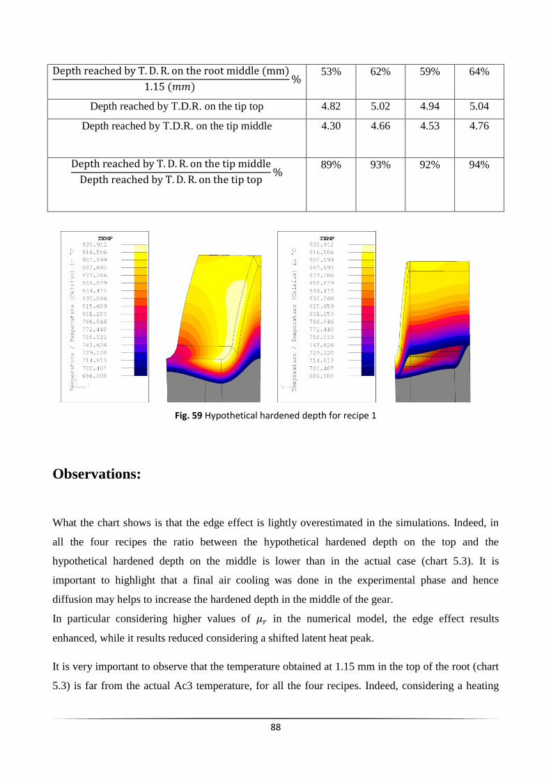
88

53% 62% 59% 64%

Depth reached by T.D.R. on the tip top 4.82 5.02 4.94 5.04

Depth reached by T.D.R. on the tip middle 4.30

4.66 4.53 4.76

89% 93% 92% 94%

Fig. 59 Hypothetical hardened depth for recipe 1

Observations:

What the chart shows is that the edge effect is lightly overestimated in the simulations. Indeed, in

all the four recipes the ratio between the hypothetical hardened depth on the top and the

hypothetical hardened depth on the middle is lower than in the actual case (chart 5.3). It is

important to highlight that a final air cooling was done in the experimental phase and hence

diffusion may helps to increase the hardened depth in the middle of the gear.

In particular considering higher values of in the numerical model, the edge effect results

enhanced, while it results reduced considering a shifted latent heat peak.

It is very important to observe that the temperature obtained at 1.15 mm in the top of the root (chart

5.3) is far from the actual Ac3 temperature, for all the four recipes. Indeed, considering a heating

89

rate of about 500°C/s for the hardened layer, Ac3 temperature should be higher. Recalling the

comparison made in the first part of this study, there is a delay in the appearance of the simulated

isotherms (figure 56 and 57). Thus, the real Ac3 temperature isotherm probably appears on delay

too, showing us a lower temperature. Moreover, after the end of the HF heating, the heat surely

flows toward the centre of the gear by conduction. Therefore this study doesn’t compare the real

hardened depth but allows us to estimate the edge effect in a numerical model.

5.6 Conclusions:

Once we have been studying the differences between numerical models and experimental results,

we can conclude that even if the present work provides a promising tool to validate simulation

models, it is difficult to properly estimate the evolution of the temperature profiles during the

induction hardening of a real gear. As a matter of fact, if one calibrate the model in order to have an

accurate temperature at a given depth for a given time, the temperature profiles tend to not be

accurate at other locations, nor at other times. On the other hand simulation well predicts the

intensity of the edge effect. Several approximations of material behaviors were tested, showing how

the simulations are sensitive to the simplifications introduced in the material descriptions.

It is necessary to do integral measurements of the machine’s parameters in order to perform a better

comparison. As a matter of fact it is not easy to estimate the actual efficiency of the hardening

machine and hence to know how much kW are really lost in the gear and in the coil. Therefore in

the simulations the power was an unknown, and hence the decision to calibrate it by reaching the

same depth of the 816°C isotherms. In this way, considering an efficiency of 0.8 of the hardening

machine, the power lost in the coil and in the gear during the simulated process just reach about

85% of the actual one. This difference may has an effect on the underestimation of the 927°C

isotherm of the simulations. As a result it is necessary for the simulations to have a precise

reference, such as the current flowing in the coil during the process.

90

91

6. Conclusion

The importance of being able to adequately simulate induction hardening processes is generally

accepted by the process development community. As a matter of fact FEM software allows the

designers to avoid a trial and error approach that is costly and time consuming, in defining the

induction hardening parameters.

The study of sensitivity presented in this work, applied to the fast induction treatment of a 4340

steel spur gear, shows the results that is possible to obtain with numerical models.

The description of relative magnetic permeability as a function of temperature and magnetic field

strength, the thermal properties of materials when exposed to high heating rates, the shift of

metallurgical transformation temperature, remain complex issues that are quite difficult to

reproduce in numerical models.

On way to validate the prediction of the electromagnetic coupled with thermal phenomena by the

simulations, the present work proposed various approximations of material behaviors, showing how

the simulations are sensitive to the simplifications introduced in the material descriptions. In

addition, the comparison with the experimental results showed how difficult it is to properly

reproduce the experimental profiles of temperatures. As a matter of fact, if one calibrates his model

in order to have an accurate temperature at a given depth for a given time, the temperature profiles

tend to not be accurate at other locations, nor at other times.

This work also shows that it would be important to have a precise reference, such as the current

flowing in the coil during the process, in order to be able to perform a better comparison.

Therefore this study should be a motivation to further improve numerical models and in particular it

would be interesting:

- To perform integral measurements of the machine’s parameters such as the current in the

coil, in order to have a precise reference for the simulations.

- To perform measurements in order to understand the real behavior of relative magnetic

permeability since there is no data in literature for AISI 4340.

92

- To develop numerical models that better describe the real behavior of the material’s

properties (relative magnetic permeability as a function of temperature and magnetic

field).

- To compare different recipes of hardening, for example with preheating phase. It should

be necessary to have lower temperature’s lacquers.

93

94

Bibliography

[1] Lupi S., "Appunti di elettrotermia", A.A. 2005-2006;

[2] Larregain B., Vanderesse N., Bridier F., Bocher P., Arkinson P., “Method for accurate

surface temperature measurements during fast induction heating”, Proceedings of the 26th

ASM Heat Treating Society Conference 2011;

[3] Lupi S., Dughiero F., Forzan M., “Modelling Single- and Double-Frequency Induction

Hardening of Gear-Wheels”. The 5th International Symposium on Electromagnetic

Processing of Materials, 2006, Sendai, Japan, ISIJ;

[4] Totten G. E., Maurice A. H. Howes, “Steel Heat Treatment Handbook”, New York, Marcel

Dekker, 11A, 11B, 1997;

[5] Ang S., Oliva A., “power switching converters”, second edition, Taylor & francis Group,

2005;

[6] Rudnev V., Metallurgical fine points of induction hardening, 2005;

[7] Rudnev V., Loveless D., Cook R., Black M., “Handbook of Induction Heating”, CRC

Taylor & Francis (2003);

[8] Candeo A. et al, “Multiphysics Modeling of Induction Hardening of Ring Gears for the

Aerospace Industry” IEEE Transactions on Magnetics, Vol. 47, No. 5 (2011), pp. 918-921;

[9] Barka N., “Etude de sensibilité du profil de dureté des engrenages traités thermiquement

par induction en foncion paramétres machine”, PhD Thesis, ETS Montréal, 2011;

[10] Billiard V., “Modélisation de la phase de refroidissement d’un procédé de trempe par

induction”, Master thesis, ETS Montréal, 2010;

[11] Spezzapria M., “Simulazione numerica del processo di tempra ad induzione di ruote dentate

per l’industria aeronautica”, Master thesis, Università Degli Studi Di Padova, 2011;

[12] Schlesselmann D., Jestremski M., Rodman D., Nacke B., “numerical simulation methods

for complex induction hardening process”, Institute of electrotechnology and Institute of

Material science, Leibniz University of Hanover;

[13] Rudnev, V., Loveless, D., Cook, R., Black, M., “Handbook of Induction Heating”, CRC

Taylor & Francis (2003);

95

[14] Martin Fisk, “Simulation of Induction Heating in Manifacturing”, Lulea University of

Technology, Department of Applied Physics and Mechanical Engineering;

[15] Miklòs Kuczmann, “Potential Formulations in Magnetics Applying the Finite Element

Method”, Laboratory of Electromagnetic Fields “Szèchenyi Istvàn”, University Gyor,

Hungary, 2009;

[16] K.D. Clarke, C.J. Van Tyne, “Effect of Prior Microstructure and Heating Rate on Austenite

Formation Kinetics in Three Steels for Induction Hardened Components”, Progress Report,

Department of Metallurgical and Materials Engineering, Colorado School of Mines, Golden,

USA, 2005;