numerical modelling for safety examination of existing concrete ...

NUMERICAL MODELLING FOR SAFETY

EXAMINATION OF EXISTING CONCRETE

BRIDGES

Mário Jorge de Seixas Pimentel

A dissertation presented to the Faculty of Engineering of the University of Porto

for the degree of Doctor in Civil Engineering.

Supervisors: Joaquim Figueiras (Full Professor); Eugen Brüwhiler (Full Professor).

ABSTRACT

In the structural safety examination of an existing bridge, the adoption of a stepwise approach is

generally recommended. As the economical impact of conservative calculations can be large and

lead to unnecessary interventions, increasing level of refinement is introduced in the structural

analysis as the assessment level progresses. This thesis aims at presenting a harmonized suit of

models with different levels of complexity that can be used in this context.

Nonlinear finite element analysis (NLFEA) is adopted as the reference method for the accurate

assessment of the load-carrying capacity of concrete structures. Since many structures can be thought

as an assembly of membrane elements, a new model for cracked, orthogonally reinforced concrete

panels subjected to a homogeneous state of stress is presented. Instead of using empirical spatially

averaged stress-strain relations, the RC panel behaviour is obtained from the contributions of each of

the physical phenomena taking place at the cracks and bond slip effects are dealt with using a

stepped rigid-plastic constitutive law. The model was found to provide good estimates of the

deformation capacity, failure loads and failure modes of a set of 54 RC panels tested under in-plane

axial and shear stresses.

A new NLFEA model based on the previously developed RC membrane element is then developed,

implemented, and validated trough comparison with the results of experimental tests on large scale

structural elements. Although the emphasis is placed on the analysis of shear critical elements, the

model is also capable of predicting the rotational capacity of plastic hinges, being thereby generally

applicable to the safety evaluation of existing bridges. Besides the ultimate loads, also crack spacing

and crack widths can be estimated with good accuracy. The implementation revealed robust and

efficient in terms of the required computational resources.

It is shown that the proposed RC membrane model can be reduced to a limit analysis formulation

through the application of some simplifying assumptions. At the cost of the loss of some generality,

the latter is more suitable for use in engineering practice and still presents good accuracy in the

calculation of the shear capacity of both continuity and discontinuity regions via the finite element

method. For the particular case of continuity regions, a sectional analysis procedure for shear

strength assessment is derived which results in a set of equations similar to those of the well known

variable angle truss model. By incorporating the longitudinal strains in the definition of the effective

concrete strength, the proposed method allows for a wider range of values for the inclination of the

struts and is suitable for an intermediate shear strength assessment of existing concrete bridges.

Finally, a case study is presented consisting of a post-tensioned box girder bridge exhibiting cracking

related pathologies. The inspection and monitoring campaigns that were developed for establishing

the bridge condition are described, as well as the numerical simulations aimed at explaining the

causes for the observed cracking patterns. The application of developed models in the safety

evaluation of the bridge is exemplified. In the case of the NLFEA, appropriate semi-probabilistic

safety formats are discussed and further developed.

RESUMO

Na análise de estruturas existentes, nomeadamente no caso das pontes, a utilização de métodos de

análise estrutural mais realistas pode ser decisiva na verificação de segurança. A abordagem que tem

vindo a ser reconhecida na regulamentação mais recente preconiza a utilização de modelos de

complexidade crescente em função das necessidades evidenciadas pelo caso em estudo. Neste âmbito,

é de todo desejável que os modelos a usar nos diversos níveis de análise estejam interligados entre si

de forma a tornar clara a sua aplicação. Esta dissertação apresenta um contributo neste domínio.

A análise não linear de estruturas é adoptada como ferramenta de referência para a avaliação do

comportamento e da capacidade resistente de elementos em betão estrutural. Neste contexto, grande

parte dos elementos estruturais podem ser idealizados como uma associação de painéis elementares

cujo comportamento é governado pelos esforços actuantes no seu próprio plano. Desta forma, na

primeira parte da dissertação é desenvolvido um novo modelo para a análise do comportamento de

painéis ortogonalmente armados sujeitos a um estado de tensão uniforme. Em vez de recorrer a leis

tensão-deformação empíricas estabelecidas com base na homogeneização das deformações medidas

em ensaios experimentais, no modelo proposto o comportamento do painel é obtido directamente a

partir da contribuição de cada um dos fenómenos que têm lugar ao nível das fendas. A aderência

entre as armaduras e o betão é modelada através de uma relação rígido-plástica, permitindo

reproduzir de forma consistente o fenómeno de retenção de tensões de tracção no betão tanto antes

como após a cedência das armaduras e, consequentemente, a obtenção de estimativas realistas da sua

capacidade de deformação. O modelo foi validado com uma base de dados contendo 54 ensaios

experimentais.

Um novo modelo constitutivo de análise não linear de estruturas foi desenvolvido para acomodar o

elemento de painel atrás mencionado. Este modelo foi implementado num código de elementos

finitos e validado através da comparação com os resultados de ensaios experimentais em elementos

estruturais de grandes dimensões. Embora tenha sido dado especial relevo à capacidade do modelo

em reproduzir roturas por corte, o modelo é também capaz de modelar a capacidade de rotação de

rótulas plásticas, não tendo portanto restrições importantes no que concerne à sua aplicabilidade.

Para além das cargas e dos modos de rotura, também o espaçamento e a abertura de fendas podem

ser reproduzidos com boa precisão. A implementação revelou ser robusta e económica em termos

dos recursos computacionais requeridos.

Partindo da formulação geral do elemento de painel anteriormente mencionada, e após vários níveis

de simplificação, chegou-se a um modelo de análise limite passível de ser utilizado na prática

corrente de engenharia estrutural para a verificação de segurança em relação ao corte. Este modelo

simplificado foi também implementado num programa de elementos finitos e permite estabelecer os

campos de tensões em condições de rotura. No caso particular das regiões de continuidade, o modelo

de análise limite foi degenerado numa formulação analítica de análise seccional. Embora seja

formalmente análogo ao método das bielas de inclinação variável preconizado na regulamentação

actual, o modelo proposto permite considerar a influência do estado de deformação das almas na

resistência ao esmagamento das bielas, e portanto na resistência ao corte.

Finalmente é apresentado um caso de estudo onde se ilustra a metodologia adoptada para efectuar a

avaliação de segurança de uma ponte rodoviária existente. Trata-se de uma ponte em betão armado e

pré-esforçado, com uma secção transversal em caixão bicelular e com um comprimento total de

250m. A ponte, com cerca de 30 anos, apresenta uma série de patologias relacionadas com a

fissuração do tabuleiro. Descreve-se sucintamente a inspecção detalhada que foi efectuada, os

principais resultados do ensaio de carga realizado e ainda os resultados das análises numéricas

efectuadas com vista a aferir as causas para a fissuração observada. A verificação de segurança é

efectuada recorrendo aos modelos desenvolvidos. Para o caso específico da análise não linear de

estruturas, novos formatos de segurança de base semi-probabilística são discutidos e desenvolvidos.

RÉSUMÉ

Lors de l'examen de la sécurité structurale du pont existant, l'adoption d'une approche par étapes est

généralement recommandée. Une fois que l'impact économique des calculs conservateurs peut être

important et conduire à des interventions inutiles, modèles d‘analyse structurale plus réalistes et

détaillées devraient être utilisés à des étapes ultérieurs. Dans ce contexte, il est souhaitable que ces

modèles à utiliser dans chaque étape soient reliés entre eux afin de préciser son application. Cette

thèse vise à présenter une ensemble harmonisé de modèles avec différents niveaux de complexité et

qui peuvent être utilisés dans ce contexte.

L´analyse non linéaire par éléments finis est adoptée comme la méthode de référence pour

l'évaluation précise de la capacité portante des structures en béton. Une fois que nombreuses

structures peut être idéalisées comme un assemblage d'éléments de membrane, un nouveau modèle

est présenté pour l‘analyse de panneaux en béton orthogonalement armées et soumis à un état de

contrainte uniforme. Au lieu d'utiliser les lois empiriques de contrainte-déformation établis après

l'homogénéisation des déformations mesurées aux essais expérimentaux, le comportement du

panneau est obtenu directement à partir de la contribution de chacun des phénomènes qui ont lieu au

niveau des fissures. L'adhérence entre l'armature et le béton est modélisé par une relation de rigide-

plastique, permettant la modélisation consistent du phénomène de rétention de contraintes de traction

dans le béton et d‘obtenir des estimations réalistes de la capacité de déformation de l‘armature. Le

modèle a été validé avec 54 essais expérimentaux.

Un nouveau modèle constitutif pour l'analyse non linéaire des structures destinées à accueillir

l'élément de panneau mentionné ci-dessus est développé. Ce modèle est implémenté dans un code

éléments finis et est validé par comparaison avec les résultats des essais sur éléments structurales de

grande dimension. Bien que mettant l'accent sur les ruptures par effort tranchant, il est également

capable de modéliser la capacité de rotation des rotules plastiques, et n'a donc pas d'importantes

restrictions quant à leur applicabilité. Aussi l'espacement et l'ouverture des fissures sont reproduites

avec une bonne précision. L‘implémentation s'est avérée robuste et économique en termes de

ressources de calcul nécessaires.

A partir de la formulation générale de l'élément de membrane mentionné ci-dessus, et après plusieurs

niveaux de simplification, un modèle d'analyse limite est développé pour être utilisé dans la pratique

du génie civil pour la vérification de sécurité contre effort tranchant. Ce modèle simplifié a été

également implémenté dans un code éléments finis et permet l‘obtention de champs de contraintes et

des charges de rupture. Dans le cas particulier des régions de continuité, le modèle d'analyse limite a

été dégénéré dans une formulation analytique d‘analyse en section. Bien qu'il soit formellement

analogue à la méthode des bielles d'inclinaison variable recommandé dans les règlements actuelles,

le modèle proposé permet d'étudier l'influence de la déformation des âmes dans la résistance au

cisaillement.

Pour terminer, on présent une étude de cas qui illustre la méthodologie adoptée pour faire

l'évaluation de la sécurité d'un pont routier existant. Il s'agit d'un pont de béton armé et précontraint

avec une longueur totale de 250m et qui présente fissuration dans le tablier. Il est décrit brièvement

l'inspection qui a été menée, les principaux résultats du test de charge ainsi que les résultats de

l'analyse numérique afin de déterminer les causes de la fissuration observée. La vérification de

sécurité est effectuée en utilisant les modèles développés. Pour le cas spécifique de l'analyse non

linéaire de structures, un nouvel format de sécurité basé sur une approche semi-probabiliste est

discuté et développé.

ACKNOWLEDGMENTS

This research work was carried out at the Laboratory of Concrete Technology and Structural

Behaviour (LABEST) of the Faculty of Engineering of the University of Porto under the

supervision of Prof. Joaquim Figueiras. I wish to express my gratitude for his support, guidance

and enthusiastic following of the work.

I would also like to thank Prof. Brühwiler, the co-supervisor of this thesis, for having welcomed me

during a 6 month stay at the Laboratory of Maintenance and Safety of Structures (MCS), in the

École Polytechnique Fédérale de Lausanne. As a result of our fruitful discussions I gained a new

and valuable insight on maintenance of the existing infrastructure.

To Prof. Mariscotti I want to express my deep gratitude for his unrelenting cooperation during the

gamma-ray inspection of the N. S. da Guia Bridge and for sharing his knowledge and experience

concerning radiographic methods for non-destructive inspection of concrete structures.

The support given by the Portuguese Foundation for Science and Technology (FCT) through the

PhD grant SFRH/BD/24540/2005 is also gratefully acknowledged.

For so many good moments spent relaxing and so many shared experiences, I would like to show

my deepest appreciation to my friends and coworkers Andrin Herwig, António Topa Gomes,

Carlos Sousa, Filipe Magalhães, Luis Borges, Luis Noites, Miguel Azenha, Miguel Castro, Miguel

Ferraz, Nuno Raposo, Pedro Costa and Xavier Romão. The friendly environment at our workplace

was very important for the success of this work.

I would also like express my profound gratitude for the unconditional love and support from my

parents and sister.

Finally, I am deeply thankful to my beloved wife Marta and newborn son Nuno for their

understanding, caring and nurturing.

Table of Contents

1 INTRODUCTION ...................................................................................................................................... 1

1.1 MOTIVATION ....................................................................................................................................... 1

1.2 OBJECTIVES ......................................................................................................................................... 3

1.3 OVERVIEW ........................................................................................................................................... 4

2 MATERIAL BEHAVIOUR ....................................................................................................................... 7

2.1 TENSILE FRACTURE .............................................................................................................................. 7

2.1.1 Tensile strength ......................................................................................................................... 7

2.1.2 Deformational behaviour .......................................................................................................... 8

2.2 BOND STRESS TRANSFER AND TENSION STIFFENING ........................................................................... 11

2.2.1 The bond-slip relation and the differential equation of bond .................................................. 12

2.2.2 Tension stiffening ..................................................................................................................... 14

2.3 SHEAR TRANSFER THROUGH ROUGH CRACKS ..................................................................................... 16

2.4 COMPRESSIVE FRACTURE ................................................................................................................... 19

2.4.1 Unixial compression ................................................................................................................ 19

2.4.2 Effect of multiaxial stresses ..................................................................................................... 22

2.4.3 Cracked concrete ..................................................................................................................... 24

3 THE RC CRACKED MEMBRANE ELEMENT .................................................................................. 29

3.1 GENERAL ........................................................................................................................................... 29

3.2 EQUILIBRIUM EQUATIONS .................................................................................................................. 30

3.2.1 Concrete contribution to shear strength .................................................................................. 33

3.2.2 Relationship between average and local crack stresses .......................................................... 33

3.3 COMPATIBILITY EQUATIONS .............................................................................................................. 37

3.4 PARTICULAR CASES ........................................................................................................................... 38

3.5 REVIEW ON PREVIOUS WORK ............................................................................................................. 39

3.6 CONSTITUTIVE RELATIONSHIPS .......................................................................................................... 48

3.6.1 Compressive behaviour ........................................................................................................... 48

3.6.2 Tensile crack bridging stresses ................................................................................................ 52

3.6.3 Shear transfer through rough cracks ....................................................................................... 52

3.6.4 Reinforcement steel and tension stiffening .............................................................................. 55

3.7 CALCULATION EXAMPLE .................................................................................................................... 62

3.7.1 F-CMM .................................................................................................................................... 65

Table of contents

3.7.2 R-CMM ..................................................................................................................................... 68

3.8 VALIDATION ....................................................................................................................................... 69

3.8.1 The influence of the reinforcement content .............................................................................. 72

3.8.2 The influence of prestressing .................................................................................................... 75

3.8.3 The influence of the concrete strength ..................................................................................... 77

3.8.4 Summary ................................................................................................................................... 81

3.9 CONCLUDING REMARKS ..................................................................................................................... 83

4 IMPLEMENTATION IN A FINITE ELEMENT CODE ..................................................................... 85

4.1 GENERAL ............................................................................................................................................ 85

4.2 COMPUTATIONAL MODELLING OF THE NONLINEAR BEHAVIOUR OF STRUCTURAL CONCRETE ............. 85

4.2.1 Kinematic description of the displacement field....................................................................... 85

4.2.2 Constitutive models and constitutive laws ................................................................................ 87

4.2.3 Discretization strategy ............................................................................................................. 89

4.2.4 Discussion ................................................................................................................................ 90

4.2.5 Solution procedures for nonlinear systems .............................................................................. 91

4.3 TOTAL STRAIN BASED MODEL ............................................................................................................. 98

4.3.1 Uncracked concrete................................................................................................................ 101

4.3.2 Cracked concrete ................................................................................................................... 108

4.3.3 Reinforcement steel ................................................................................................................ 123

4.4 EXTENSION TO SHELL ELEMENTS ...................................................................................................... 133

4.5 CONCLUDING REMARKS ................................................................................................................... 135

5 ANALYSIS OF SHEAR CRITICAL ELEMENTS ............................................................................. 137

5.1 GENERAL .......................................................................................................................................... 137

5.2 SHEAR IN CONTINUITY REGIONS ....................................................................................................... 138

5.2.1 Description and objectives ..................................................................................................... 138

5.2.2 Results .................................................................................................................................... 140

5.3 SHEAR IN DISCONTINUITY REGIONS WITH PLASTIC REINFORCEMENT STRAINS .................................. 145


5.3.2 Results .................................................................................................................................... 148

5.4 HIGH STRENGTH CONCRETE GIRDERS CRITICAL IN SHEAR................................................................. 155


5.4.2 Results .................................................................................................................................... 158

5.5 ANALYSIS OF THE DEFORMATION CAPACITY OF PLASTIC HINGES WITH HIGH SHEAR STRESSES ......... 164


5.5.2 Results .................................................................................................................................... 167


Table of contents

6 SIMPLIFIED MODELS FOR ENGINEERING PRACTICE ............................................................ 173

6.1 GENERAL ......................................................................................................................................... 173

6.2 LIMIT ANALYSIS METHODS FOR STRUCTURAL CONCRETE ELEMENTS SUBJECTED TO IN-PLANE FORCES

174

6.2.1 Overview and general considerations ................................................................................... 174

6.2.2 Yield conditions of reinforced concrete membranes .............................................................. 176

6.2.3 Yield conditions accounting for compression softening ........................................................ 178

6.2.4 Continuous stress fields ......................................................................................................... 183

6.2.5 Discontinuous stress fields .................................................................................................... 186

6.2.6 Section-by-section analysis for continuity regions ................................................................ 195

6.3 CODE-LIKE FORMULATION ............................................................................................................... 197

6.3.1 Proposed expressions ............................................................................................................ 198

6.3.2 Sample calculations ............................................................................................................... 201


7 CASE STUDY: N. S. DA GUIA BRIDGE ............................................................................................ 209

7.1 DESCRIPTION OF THE BRIDGE AND PROBLEM STATEMENT ................................................................ 209

7.2 AVAILABLE DATA ............................................................................................................................ 211

7.3 INSPECTION ...................................................................................................................................... 213

7.3.1 Mapping of the cracking patterns .......................................................................................... 213

7.3.2 Corrosion evidence ................................................................................................................ 217

7.3.3 Verification of the reinforcement layout ................................................................................ 217

7.3.4 Trial test using gamma rays .................................................................................................. 218

7.4 MATERIAL CHARACTERIZATION ...................................................................................................... 225

7.4.1 Concrete ................................................................................................................................ 225

7.4.2 Reinforcing steel .................................................................................................................... 229

7.4.3 Prestressing steel ................................................................................................................... 229

7.5 MONITORING CAMPAIGN .................................................................................................................. 229

7.5.1 Load test ................................................................................................................................ 232

7.5.2 Response to temperature variations ...................................................................................... 236

7.6 INVESTIGATION OF THE CAUSES FOR THE OBSERVED CRACKING PATTERNS ..................................... 237

7.6.1 Stress analysis in serviceability conditions ........................................................................... 237

7.6.2 Effect of local stress conditions ............................................................................................. 252

7.7 DISCUSSION ..................................................................................................................................... 261

8 SAFETY EVALUATION OF THE N. S. DA GUIA BRIDGE ........................................................... 263

8.1 GENERAL ......................................................................................................................................... 263

8.2 SAFETY FORMAT FOR NONLINEAR ANALYSIS OF EXISTING BRIDGES ................................................. 265

8.2.1 Basic reliability concepts ....................................................................................................... 265

Table of contents

8.2.2 Global resistance safety factor ............................................................................................... 268

8.2.3 Target reliability index ........................................................................................................... 273

8.2.4 Application to NLFEA of existing bridges .............................................................................. 275

8.3 STRUCTURAL SAFETY EVALUATION OF THE N. S. DA GUIA BRIDGE ................................................. 276

8.3.1 Definition of the target reliability index ................................................................................. 276

8.3.2 Updated examination values .................................................................................................. 278

8.3.3 Linear elastic analysis – member level approach .................................................................. 279

8.3.4 Nonlinear analysis ................................................................................................................. 280

8.3.5 Continuous stress field analysis ............................................................................................. 290


9 SUMMARY AND CONCLUSIONS ..................................................................................................... 295

9.1 RECOMMENDATIONS FOR FUTURE RESEARCH ................................................................................... 301

REFERENCES ................................................................................................................................................. 305

APPENDIX – DETAILED VALIDATION RESULTS ................................................................................ 319

A1.1 – ISOTROPICALLY REINFORCED CONCRETE PANELS ........................................................................... 319

A1.1.1 – Series A .................................................................................................................................. 319

A1.1.2 – Series VA ................................................................................................................................ 320

A1.1.3 – Series PV ................................................................................................................................ 321

A1.2 – ORTHOTROPICALLY REINFORCED CONCRETE PANELS ..................................................................... 322

A1.2.1 – Series B .................................................................................................................................. 322

A1.2.2 – Series PP ................................................................................................................................ 325

A1.2.3 – Series SE ................................................................................................................................ 327

A1.2.4 – Series VB ................................................................................................................................ 328

A1.2.5 – Series M.................................................................................................................................. 330

A1.2.6 – Series PV ................................................................................................................................ 332

1

1 Introduction

1.1 Motivation

The built infrastructure, of which bridges are an important component, is a hugely valuable

economic and political asset. Its maintenance, repair and renewal constitute a heavy burden

for society. For the existing highway bridge stock in all 27 countries of the European

Union, the total expenditure was estimated at €400 billion [66] in 2004, which was roughly

4% of the Gross Domestic Product. Due to the large sums involved, the financing of

maintenance, repair and renewal needs to be put on a rational basis. There is consensus

regarding the need for specific procedures for the assessment of existing bridges and the

importance of adequate bridge management strategies. This is crucial for minimizing and

rationalizing the increasingly growing maintenance costs and associated traffic

disturbances, for contributing to environmental sustainability and for ensuring the adequate

safety levels to the infrastructure users.

In the final report of the BRIME research program [36], devoted to the development of a

framework for the management of bridges on the European road network, it is proposed

that a general Bridge Management System (BMS) should be constituted by 5 main

components: (1) an inventory database; (2) a suite of procedures for assessing bridges

condition; (3) methods for performing the structural safety assessment; (4) a decision

making procedure for determining whether a sub-standard or deteriorated bridge should be

repaired, strengthened or replaced; and (5) some prioritization criteria for deciding the best

allocation of the limited financial resources. Structural engineering plays a major role in all

these components and especially in components 2 and 3. In fact, the key for extending the

service life of an existing bridge is a detailed examination of its condition and an accurate

structural safety evaluation, thereby requiring a completely different approach than the

traditionally adopted in the design of a new bridge.

In design and construction of new structures a great effort must be placed on the

conceptual design, on the choice of the appropriate structural form and its aesthetics, on the

analysis of the local conditions, on the selection of the construction methods and materials

and on the feasibility of the proposed solution. Many solutions have to be tested until the

Chapter 1

2

final design is achieved. The analytical work is only part of the process and usually simple

methods are preferred, enabling quick estimates of the internal forces and conservative

estimates of the actual resistance. Design codes are available for guiding the structural

engineer throughout the required safety checks, indicating the load models to be adopted,

the material properties, the design formulas and the appropriate safety format. The latter is

usually based on a semi-probabilistic approach grounded on a uniform target safety level,

independent of the structural element being designed. In most cases, the additional cost due

to a conservative design is not very significant [155] and this procedure is shown to be

adequate.

On the other hand, in the assessment of an existing bridge advantage must be taken from

the fact that the bridge can be inspected, tested and monitored during load testing or under

traffic and environmental actions. The structural engineer should resort to more detailed

structural analysis methods since the economical impact of conservative calculations can

be large and lead to unnecessary interventions, and because the structural condition can be

established based on appropriate testing and inspection techniques. If necessary, the load

models can be updated taken into account local traffic conditions and risk based

approaches can be used to define the target safety level taking into account the identified

hazard scenarios and the corresponding consequences with respect to damage and

economic importance of the bridge. This process requires comprehensive knowledge of

structural engineering beyond the scope of design codes and supplies sufficient motivation

and economical benefits for the application of advanced numerical methods and the latest

accepted scientific findings.

Whilst in recent decades considerable effort has been put into the development of new

standards for the design of new structures, comparatively less has been done on the

development of guidance documents addressing the assessment of existing structures. In

the case of bridges, several research programmes funded by the European Commission

have been undertaken for filling this gap [36; 66; 202; 258; 259]. In general a stepwise

approach is recommended [36; 66; 259] to identify which bridges are at an unacceptably

high level of risk so that appropriate remedial measures can be taken. In the case of the

structural analysis, increasing level of refinement is introduced as the assessment level

progresses. Although this line of thinking is already reflected in recent codes [87], there is

still work to be developed regarding the establishment of suitable analysis methods that

can be used in such a context. The simpler methods should preferably be based on the

more detailed ones through transparent simplifying assumptions in order to keep clarity

Introduction

3

and consistency between the results obtained in the successive levels of analysis. This

thesis aims at presenting a contribution in this field.

1.2 Objectives

Nonlinear finite element analysis (NLFEA) is increasingly recognized as an effective tool

for the accurate assessment of the load-carrying capacity of concrete structures [86]. By

enabling the consideration of both equilibrium and compatibility conditions, and if

appropriate constitutive laws are adopted, realistic force-deformation relationships and

ultimate loads can be calculated. Within the NLFEA context, many structural concrete

elements, such as bridge I-girders and box-girders, shear walls, transfer beams,

containment structures and offshore oil platforms, to cite a few, can be idealized as an

assembly of membrane elements subjected mainly to in-plane shear and axial forces.

Therefore, the accurate representation of the structural concrete behaviour at the membrane

element level is here taken as the starting point for the detailed analysis of structural

concrete elements with arbitrary geometry via the finite element method.

In this context, the first objective of this thesis is the development of a strict reinforced

concrete (RC) cracked membrane element formulation, in the sense that the mechanical

phenomena taking place at the cracks, and which are known to govern the behaviour of

cracked concrete elements, are taken into account in a transparent manner. The main

features of the structural concrete behaviour, such as tensile cracking, compression

softening, shear stress transfer between rough cracks and bond interaction with the

reinforcement shall be explicitly considered in the formulation. The model shall describe

the complex stress and strain fields developing in the membrane element, and retrieve

useful information for the structural engineer, such as concrete and reinforcement failures

as well as the crack spacing and crack widths.

The second objective of the thesis is the implementation of the above mentioned RC

cracked membrane element formulation in a finite element code, thereby constituting an

advanced analysis tool allowing detailed safety examinations of concrete structures. The

implementation shall be robust in order to minimize the convergence difficulties that often

discourage the use of nonlinear analysis methods. Short-term static loading is assumed,

excluding dynamic or cyclic loads as well as long-term and material degradation effects.

Chapter 1

4

The third objective is the development of simplified formulations suited for use in

engineering practice. In fact, practitioner structural engineers are seldom familiar with

nonlinear analysis concepts and do not have the vocation to deal with the great amount of

information provided by nonlinear finite element analysis tools. These simplified

formulations shall be traced back to the previously outlined detailed models through clear

simplifying assumptions, so as to make them part of an integrated and stepwise structural

assessment procedure. Since flexural strength can be considered to be satisfactorily

predicted in current design methods, the focus of these simplified formulations shall be

driven to shear dominated problems.

The last and fourth objective is the safety examination of a real bridge and the application

of the developed structural analysis tools in a case study. The available safety formats

suitable for nonlinear analysis shall be applied and further developed.

1.3 Overview

In Chapter 2 the fundamental concepts related with concrete behaviour under short term

loading conditions and its interactions with the reinforcement are introduced. These

concepts and terminology are used throughout the thesis, namely in Chapters 3, 4 and 6.

In Chapter 3 the development and validation of a new formulation describing the

behaviour of RC cracked membrane elements is presented. Rather than using empirical and

spatially averaged stress-strain relations, in the proposed formulation RC behaviour is

described taking into account the individual contribution of the mechanical phenomena

taking place at the cracks. Bond slip effects are dealt with using a stepped rigid-plastic

constitutive law according to the Tension Chord Model [151] which allows for a consistent

treatment of the tension stiffening effects and a proper evaluation of steel deformation

capacity in the post-yielding stage. After having introduced the general equilibrium and

compatibility equations governing the problem, and having analysed in detail the complex

stress field developing at the cracks and in between the cracks, the relationship between the

different existing approaches are clarified and the previous work on this field is critically

reviewed. The adopted constitutive relationships are presented and the results obtained

with the developed model are evaluated using a database of 54 experimental tests on RC

panels under in-plane shear and axial forces. The influences of the reinforcement content,

prestressing force and concrete strength on the behaviour of RC panels are examined in

detail.

Introduction

5

In Chapter 4, the RC cracked membrane element formulation is further developed to be

used in the structural analysis via the finite element method. The concepts behind NLFEA

of concrete structures are introduced and a short overview of the existing approaches is

presented. In addition to the work described in Chapter 3, the implementation in a finite

element code requires the formulation of concrete nonlinear behaviour in biaxial

compression, the establishment of suitable loading/unloading conditions, the generalization

of the shear stress transfer model to cases where two orthogonal cracks arise in the same

integration point, the treatment of strain localization issues and the formulation of the

tangent stiffness matrix to be used in the incremental-iterative solution procedure. The

structure of the code is presented, as well as the implemented algorithms. Some single

element validation examples are presented to clarify the model behaviour under complex

loading histories. In order to enlarge the range of applicability of the proposed model, the

formulation is extended to shell elements.

In Chapter 5 the analysis of large scale structural concrete elements is performed for

validation purposes and for illustrating the model capabilities. The analysed examples were

selected for evaluating the accuracy of the model in the: (1) calculation of shear failure

loads and corresponding failure mechanisms; (2) determination of the load-deformation

curves and of the deformation capacity of large scale beams; (3) simulation of the observed

cracking patterns and calculation of the corresponding crack widths. Each of the selected

test series represents a specific feature of the structural behaviour that should be properly

modelled in order to allow improved structural analyses of existing concrete bridges.

In Chapter 6 the derivation of simplified formulations for engineering practice is presented.

Starting from a particular case of the equilibrium equations of the RC cracked membrane

element, neglecting the tensile strength and the bond stress transfer effects, and considering

simple rigid-plastic relations for concrete and steel, the classical closed form limit analysis

expressions for shear strength calculation of RC panels are derived. Following the work

developed by Kaufmann [117], these expressions are then worked out to include the effect

of the tensile strains in the effective concrete compressive strength, thus allowing to

include strain compatibility conditions in shear strength calculations. Besides improving

the accuracy of the classical limit analysis expressions, this formulation can be easily

implemented in a finite element code in such a way that is more suitable to be used in

engineering practice than the detailed models developed in Chapters 3 and 4. However, the

relevant outcomes are simply the continuous stress field expressing the equilibrium at

failure conditions and the corresponding ultimate load. A simple sectional analysis method

Chapter 1

6

for beam continuity regions is derived from the same set of expressions but considering a

constant shear stress distribution along the cross-section height, thus avoiding the resource

to finite element analyses in cases where a sectional analysis approach is deemed sufficient.

In Chapter 7, a case study is presented consisting of a 30-years old and 250 m long post-

tensioned box-girder bridge exhibiting cracking patterns with both longitudinal and

transversal symmetry. The inspection and monitoring campaigns that were developed for

establishing the structural condition of the bridge are described, as well as the numerical

analyses aimed at explaining the origin of the observed cracking patterns.

In Chapter 8 the safety evaluation of the bridge with resource to the models developed in

the present thesis is presented. The chapter begins by giving an overview on the applicable

safety formats whenever nonlinear analysis concepts are adopted, and by showing how to

define a global resistance factor based on semi-probabilistic concepts that can capture the

resistance sensitiveness to the random variation of the input variables. A stepwise approach

is adopted in the structural safety evaluation illustrating the applicability of the developed

models in each assessment stage.

Finally, Chapter 9 summarises and discusses the results obtained in this thesis and

concludes with a set of recommendations for future research.

7

2 Material behaviour

2.1 Tensile fracture

2.1.1 Tensile strength

Concrete tensile strength fct is relatively low when compared to the compressive

strength cf , is subject to high scatter and is significantly affected by additional factors like

restraining shrinkage stresses. Therefore, it is common practice to neglect it in strength

calculations of properly reinforced concrete members. However, shear resistance of some

structural elements, like girders or slabs without stirrups, relies on the existence of concrete

tensile stresses [27; 63; 166]. The consideration of concrete tensile stresses allows

explaining the strong size effects that have been reported in shear failures of beams without

shear reinforcement [18; 62]. Concrete tensile behaviour also plays a key role in important

aspects related with serviceability considerations, like the quantification of the

deformations, assessment of crack spacing and crack widths. Moreover, the evaluation of

the reinforcing steel deformation capacity – which is essential for an accurate calculation

of the force-deformation curves, failure modes and, in case of statically indeterminate

structures, of the failure loads – can only be evaluated if due consideration is given to the

concrete tensile behaviour and to the bond shear stress transfer mechanics.

The tensile strength can be determined from direct tension tests or by means of indirect

tests such as the split cylinder test, double punch test or bending test. While easier to

perform these indirect tests require assumptions about the state of stress within the

specimen in order to calculate the tensile strength from the measured failure load. For most

purposes, the tensile strength of normal strength concrete can be estimated from [46],

3/23.0 cct fkf [MPa] (2.1)

where the parameter k varies between 0.65 and 1 and allows for the effect of non-uniform

self equilibrating stresses leading to a reduction of the ―apparent‖ tensile strength. This

parameter introduces a structural effect on fct since it depends on the specimen thickness,

Chapter 2

8

reinforcement content, etc. Alternatively, a lower bound estimate, already accounting for

the self equilibrated residual stresses, can be obtained from [20; 240]:

cct ff 33.0 [MPa] (2.2)

2.1.2 Deformational behaviour

The stress-strain response depicted in Figure 2.1 (a) can be typically obtained in a

displacement controlled direct tension test. Until stress levels near the tensile strength the

response is approximately linear elastic. Near the peak load the response becomes softer

due to micro-crack growth at the interface between the aggregates and the cement paste.

As the tensile strength is reached, deformations begin to appear heavily localized in a

narrow band, the so called fracture process zone (FPZ) [17], and the micro-cracks start

coalescing into a macroscopic crack. Tensile stresses can still be transmitted due to crack

bridging effects [102] and a strain-softening behaviour can be observed. At this stage the

deformations are highly localized, the specimen unloads outside of the FPZ and the

measured softening branch can be more or less steep, depending on the base length that is

used for averaging the deformations. At the macro-level, this behaviour cannot be

explained by regular continuum mechanic models neither by linear elastic fracture

mechanics (LEFM), requiring the application of nonlinear fracture mechanics (NLFM)

concepts. It must be remarked that the softening behaviour does not exist in a

heterogeneous material like concrete if its micro or meso-structure is considered with

sufficient resolution, being only a mere homogenization product at the macro-level [9].

The NLFM models can be classified according to the assumed localization criteria for the

deformations in the softening regime [75] (see Figure 2.1 (b)-(d)).

(a) (b) (c) (d)

Figure 2.1 – Tension softening and localization criteria for the deformations in the softening regime: (a)

behaviour of a tensioned concrete specimen; (b) FPZ lumped into a line – fictitious crack model [99]; (c)

deformations localized in a band of finite length – crack band model; (d) continuous strain field - non local

continuum models.

Material behaviour

9

Hillerborg [99] introduced the fictitious crack model for describing the observed behaviour

of concrete in tension. In this model the FPZ is lumped to a line, the fictitious or cohesive

crack, which is still capable of transmitting stresses (Figure 2.2). According to the

fictitious crack model the total elongation of a specimen subjected to pure tension is

given by Eq. (2.3), where Lt is the total specimen length, c is the concrete strain outside

the FPZ and w is the elongation in the FPZ.

wLtc (2.3)

The average specimen strain m can be calculated from:

tcm Lw (2.4)

As shown in Eq. (2.4) the fictitious crack model can successfully explain the size

dependency of the -m curve after the tensile strength is reached, i.e., when w>0. After the

beginning of strain localization the -m curve is no longer a material property. The

uniaxial tensile constitutive relationship is then expressed by two curves: (1) a stress-strain

curve-c for the concrete outside the FPZ; (2) a stress-elongation curve -w for the FPZ.

The consideration of the -w relation as a material property leads to the definition of a

material parameter defined by the area of the -w diagram. This parameter, that Hillerborg

named as fracture energy, GF [N∙m-1

], corresponds to the energy required for the formation

of a macroscopic crack with unit area,

cw

F dwG0

(2.5)

where wc is the fictitious crack opening at which the tensile stress drops to zero.

The fracture energy depends primarily on water/cement ratio, maximum aggregate size

Dmax and age of concrete [84]. As a rough approximation GF can be estimated from [84]:

7.0

010

c

FF

fGG for 80cf MPa

030.4 FF GG for 80cf MPa

(2.6)

where GF0 = 25, 30 or 58 N∙m-1

for Dmax = 8, 16 or 32 mm respectively.

Chapter 2

10

(a) (b)

Figure 2.2 – Fictitious crack model: (a) crack bridging stresses in the fictitious crack; (b) components of

the total deformation.

Bazant and Oh [17] introduced the crack band model. In this model strains are assumed to

localize in a finite length FPZ, following a uniform distribution. The crack band model

introduces the crack band width ht as a new parameter, representing the width over which

the FPZ deformations are averaged. This averaging process corresponds to the simplest

homogenization procedure of the real strain distribution enabling treating a heterogeneous

material like concrete as a continuum. The constitutive relationships for the crack band

model are illustrated in Figure 2.3. For the concrete inside the FPZ the constitutive

relationship is a function of fct, GF and ht. A parallelism with the fictitious crack model can

be established by defining the crack strain as cr = w / ht, being the fracture energy now

defined by:

ucru

crtttF dhLdhG,

00

(2.7)

Figure 2.3 – Crack band model. Notation.

Material behaviour

11

The crack band model supplies the theoretical background allowing the application of

NLFM concepts within a continuum mechanics framework, thus enabling the use of

standard continuum finite element models in cases where strain localization in a few

narrow zones governs the structural behaviour. This will be discussed in more detail in

Chapter 4. More powerful and generic continuum descriptions (see Figure 2.1(d)), which

include a so called internal length defining the (non-zero) width of the localization zone,

were developed after the crack band model. Such enhanced continuum theories include the

Cosserat continuum (see e.g. [31]), the non-local continuum with integral averaging of

strain (see e.g. [14; 16]) and the high order gradient continuum (see e.g. [33]). A detailed

description of such theories is out of scope of the present work.

2.2 Bond stress transfer and tension stiffening

Bond between reinforcement and concrete is a fundamental issue in the study of structural

concrete behaviour. After cracking, relative displacements between concrete and

reinforcement occur leading to the development of bond stresses at the steel-concrete

interface.

In the case of plain reinforcing bars, bond action is mainly governed by adhesion. After

breakage of the adhesive forces, which occurs for very low relative displacements, force

transfer is provided by dry friction. In the case of ribbed bars, bond action is primarily

governed by bearing of the ribs against the surrounding concrete and forces are transmitted

to concrete by inclined compressive forces radiating from the bars. These bearing forces

can be decomposed in the parallel and radial directions to the bar axis. The sum of parallel

components equals the bond force, whereas the radial components are balanced by

circumferential tensile stresses in the concrete or by lateral confining stresses. The latter

can be provided by circumferential reinforcement. If significant forces have to be

transmitted over a short length from steel to the embedding concrete, splitting failures

along the reinforcement will occur unless sufficient concrete cover or proper confinement

is provided. This effect is called tension splitting. For a detailed discussion about the bond

phenomenon refer to references [3; 84; 85; 214].

The complex mechanism of bond stress transfer can be studied at different levels with

regard to the size of the control volume [137]. In the most common approach, the problem

is simplified by considering a nominal bond shear stress uniformly distributed over the

Chapter 2

12

nominal perimeter of the reinforcing bar. In this case, the control volume can be assumed

to be the finite domain between two consecutive cracks.

2.2.1 The bond-slip relation and the differential equation of bond

Average bond shear stress-slip relationships, b , are normally obtained from pull-out

tests, see Figure 2.4 (b) and (a), respectively. The average bond shear stress, b , along the

embedment length, lb, can be determined from the pull-out force as b = F / Ø lb, where Ø

is the nominal rebar diameter. In a pull-out test, bond shear stresses increase with the slip

until the maximum bond shear stress maxb is reached. This typically occurs at a slip

= 0.5…1 mm. If the slip is further increased, bond shear stresses decrease, as shown in

the curve depicted in Figure 2.4 (b). In general this curve represents a structural behaviour

since it depends on the concrete cover, on the existence of confinement stresses, type of

reinforcing bar, etc.

(a) (b) (c)

Figure 2.4 – (a) Pull-out test; (b) Average bond shear stress-slip curve; (c) Equilibrium of a differential

element.

Consider a concrete element loaded in uniform tension, Figure 2.4 (c). For any section of

the element, equilibrium requires that:

cs

sA

N

1 (2.8)

where cs AA is the reinforcement ratio, As is the cross sectional area of reinforcement ,

Ac is the gross cross-section of concrete, and c and s are the concrete and steel stresses,

respectively. Formulating the equilibrium of the differential element of length dx, see

Figure 2.4 (c), one obtains the relations,

Material behaviour

13

bs

dx

d 4

dx

d

dx

d sc

1 (2.9)

for the stresses transferred between concrete and reinforcement by bond. Noting that

= us - uc, the kinematic condition is obtained:

csdx

d

(2.10)

The second order differential equation for the slip is obtained by differentiating (2.10)

with respect to x, inserting (2.9) and substituting the stress-strain relationships for steel and

concrete. For linear elastic behaviour, s = Ess and c = Ecc, the equation simplifies to:

11

42

2 n

Edx

d

s

b (2.11)

where is the geometrical reinforcement ratio and n is the modular ratio Es/Ec.

Adopting a bond shear stress-slip relationship b , the differential equation (2.11) can

be solved in an iterative numerical manner [3; 214], and the distributions of the stresses,

strains and slip along the reinforcing bars can be obtained. Such distributions are

qualitatively depicted in Figure 2.5 for the stabilized cracking stage. The dotted lines refer

to the pre-yielding stage whereas the solid lines refer to the post-yielding stage. In the pre-

yielding stage the steel stresses at the cracks sr are below the steel yielding stress fsy. After

reinforcement yielding strong strain localizations are observed in the vicinity of the cracks.

(a) (b)

Figure 2.5 – (a) Tension chord element. (b) Qualitative distribution of bond shear stresses, steel and

concrete stresses and strains, and bond slip.

Chapter 2

14

The crack width wr can be calculated by integrating Eq. (2.10) between two consecutive

cracks

rs

csr dxw0

(2.12)

with sr being the crack spacing.

2.2.2 Tension stiffening

In a cracked concrete cross-section, all tensile forces are resisted by the reinforcing bars.

As discussed above, between adjacent cracks these forces are partially transmitted from the

steel to the surrounding concrete by bond stresses. At the structural level, the effect of the

concrete contribution between the cracks on the behaviour of a structural concrete tension

chord is reflected by a stiffer load-displacement response than that of a naked steel bar of

equal resistance, see Figure 2.6. This effect is called tension stiffening.

Tension stiffening is automatically accounted for if the slip between the reinforcing bars

and the surrounding concrete is explicitly considered and proper bond shear stress-slip

relationships are adopted, as outlined previously. In general, this procedure requires the

solution of the second order bond-slip differential equation via an iterative numerical

method. However, simpler formulations can be obtained if the bond stress-slip law is

chosen such that the integration of the differential equation is simplified. A formulation of

this type is going to be adopted in this work and will be further detailed in Chapter 3.

Figure 2.6 –Tension stiffening.

Condition (2.15)

Material behaviour

15

When the control volume over which the constitutive laws are established is enlarged to

include several cracks, the so called tension stiffening curves are frequently used to

directly relate the average concrete tensile stress cm with the average tensile strains sm,

see Figure 2.6. In this case, both the stress and strain fields are spatially averaged within

the control volume and the stress and strain distributions between the cracks are not

explicitly considered. These spatially averaged relationships are valid if the reinforcement

ratio is higher than the minimum, ensuring that yielding does not occur immediately after

cracking. In these circumstances, a distributed stabilized cracking pattern is formed and the

explicit consideration of the strain localization issues mentioned in Section 2.1 can be

disregarded in the structural analysis.

The average tensile response of cracked reinforced concrete can be obtained directly from

tests on tensioned structural concrete members [21] or from equilibrium considerations

based on idealized concrete tensile stress distributions between the cracks [40; 84]. Other

authors establish the tension stiffening curve from tests on RC panels subjected to in plane

shear and axial stresses [25; 240]. However, the tension stiffening diagrams obtained in

this way cannot be determined simply from equilibrium equations and are based on a series

of assumptions, as will be shown in Chapter 3. Therefore, the obtained diagrams reflect the

theory used in assessing the experimental results and may mask other mechanical effects.

When using a tension stiffening diagram for calculating the response of a tensioned

structural concrete member, a suitably spatially averaged relationship for the reinforcement

steel must be adopted. If Eq. (2.8) is written in terms of averaged quantities it is possible to

conclude that:

cmsmsr

sA

N

1 (2.13)

When the load is increased such that reinforcement yielding occurs at the crack location,

i.e. sr = fsy, one obtains

cmsysy ff

1

(2.14)

where

syf is the average yield stress, i.e. the average stress in the reinforcing bars

corresponding to the occurrence of the first yield at the cracks, see Figure 2.6. This average

Chapter 2

16

yield stress depends on the adopted tension stiffening diagram. In references [21; 137]

suitable averaged stress-strain relationships for the embedded bars are proposed.

Some authors use the bare bar stress-strain relationship. In these circumstances the adopted

tension stiffening diagram must fulfil the condition:

smsycm f

1 (2.15)

In this case, tensile stresses carried by concrete in the post yielding stage are disregarded

and the deformation capacity of the structural members is not properly evaluated, as can be

seen in Figure 2.6.

The crack widths can still be calculated using this averaged approach by estimating the

crack spacing sr and expressing the integral relationship (2.12) in terms of the average

strains and average concrete stresses:

c

cmsmrr

Esw

(2.16)

2.3 Shear transfer through rough cracks

The last stage of the tensile fracture process corresponds to the formation of a macroscopic

crack that cannot transmit normal stresses. Shear transfer across these cracks cannot be

simply formulated as a relation between shear stress and shear displacement, but is a more

complex mechanism, in which shear stress, shear displacement, normal stress and crack

width are involved. Several models have been proposed for reproducing the shear transfer

mechanisms through the rough crack lips. Some of these models arise from a physical

description of the material behaviour at the mesoscale level (via the mechanics of the crack

surface contacts), while others result from more or less empirical fits to a set of

experimental results. For a review of the existing proposals refer to references [13; 37; 41;

133; 251]. The experimental tests consist essentially in the application of shear forces

along previously cracked surfaces – the push off test – varying the crack width, the

confinement degree and the loading path (Figure 2.7).

Material behaviour

17

Figure 2.7 – Shear transfer through rough cracks: (a) push off test setup; (b) notation.

-10

-8

-6

-4

-2

0

2

4

6

8

10

0 0.5 1 1.5 2

r,t [mm]

[MP

a]

Series15

d

il a

gg

w r =1.0 mm

0.3

0.6

0.1

-10

-8

-6

-4

-2

0

2

4

6

8

10

0 0.5 1 1.5 2

r,t [mm]

[MP

a]

Full

d

il a

gg

w r =1.0 mm

0.30.6

0.1

(a) (b)

-10

-8

-6

-4

-2

0

2

4

6

8

10

0 0.5 1 1.5 2

r,t [mm]

[MP

a]

Series15

dil

agg

w r =1.0 mm

0.3 0.60.1

-10

-8

-6

-4

-2

0

2

4

6

8

10

0 0.5 1 1.5 2

r,t [mm]

[MP

a]

Series15

dil

agg

w r =1.0 mm

0.30.6

0.1

(c) (d)

Figure 2.8 – Simulation of a push off test under controlled wr : (a) Aggregate interlock relation by

Walraven [251] combined with the crack shear capacity expression proposed by Vecchio and Collins

[240]; (b) Contact density model by Li et al. [133]; (c) Rough crack model by Bazant and Gambarova

[12]; (d) Rough crack model by Gambarova and Karakoç, according to [23; 257].

In normal strength concrete (NSC) cracks propagate essentially along the interface

between the hardened cement paste and the aggregate particles, originating a highly

irregular macroscopic fracture surface. When a crack is subjected to a shear displacement

aggregates are pushed against its negative in the hardened cement paste and both normal

and frictional forces can be transmitted in numerous contact surfaces. Aggregate particles

are generally stiffer than the cement paste, which crushes locally at the contact surfaces,

Chapter 2

18

producing a highly inelastic macroscopic behaviour. The crack roughness is also

responsible for a dilating behaviour that is manifested as follows (see Figure 2.7 for

notation): keeping the normal confinement stress dil constant, a shear stress agg will

produce a shear displacement r,t and an increase in the crack opening r,n (or wr); keeping

r,n constant, a shear stress agg will produce a shear displacement r,t and an increase of

the confinement stress dil. With increasing crack opening, the contact zones between the

opposite crack faces will diminish and the transmitted shear force decreases with

increasing r,n. For large values of r,t large degradation of the crack surface may occur and

the transmitted shear force tends to stabilize, or even decrease, after a certain r,t threshold

value. In Figure 2.8 the simulation of a push off test under controlled wr according to

several theoretical models is presented. A concrete strength of 30cf MPa and a

maximum aggregate size Dmax=16mm were adopted. From the theoretical models available

in the literature, only the ones for which a closed form solution is possible, at least for the

monotonic load path, were chosen.

For similar fracture surface typologies, the crack shear strength increases with the concrete

strength. However, in high strength concrete, cracks propagate through the aggregate

particles and the crack surfaces tend to be smoother. Although there is experimental

evidence that shear transfer capacity may be reduced, still significant shear forces can be

transmitted through high strength concrete cracks. Walraven [251] reported less shear

dilatancy for high strength concrete specimens, which indicates higher preponderance of

the frictional stresses as load carrying mechanisms, when compared to normal strength

concrete.

Cracks crossed by bonded reinforcement exhibit a distinct behaviour, which cannot be

solely attributed to dowel action effects. Compared to the results of similar tests in

specimens with interrupted bond in the neighbourhood of the crack or in specimens with

external restraints, Walraven [251] observed a stiffer response, more crack shear dilatancy

and that the crack opening direction was almost independent of the reinforcement content.

These differences were attributed to the reduction of the crack width near the

reinforcements due to bond stress action, leading to the formation of compressive struts

which are responsible for an additional load carrying mechanism (Figure 2.9 (a)). This

effect was important for reinforcement contents larger than 0.56%. Walraven proposed a

physical model for this effect involving the consideration of a system of stiff hinged struts

connecting the crack lips. The polygon of forces expressing the equilibrium in the crack

plane is represented in Figure 2.9 (b).

Material behaviour

19

(a) (b)

Figure 2.9 – Shear transfer through steel reinforced cracks: (a) expected additional cracking and load

carrying mechanism in the case of bonded deformed bars; (b) equilibrium of forces (Fext is the applied

shear force, Fdowel is the force due to dowel action, Fs is the sum of the reinforcement forces, Fagg is the

force due to aggregate interlock, Fdil is the corresponding dilatancy force and Fstruts is the additional force

required to close the polygon).

2.4 Compressive fracture

2.4.1 Unixial compression

Uniaxial compressive strength

The response of concrete in uniaxial compression is usually obtained from cylinders with a

height to diameter ratio of 2. The standard cylinder is 300mm high by 150mm in diameter

and the resulting compressive strength is here denoted by cf . Smaller cubes are commonly

used for production control. The cube strength is higher than the obtained from standard

cylinders since the end zones of the specimens are laterally constrained by the frame

loading plates and the state of stress in the failure zone cannot be considered purely

uniaxial.

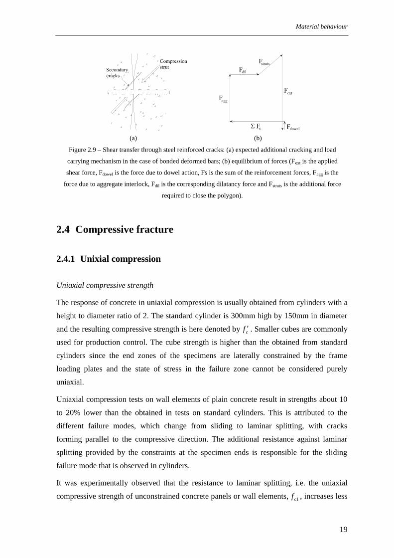
Uniaxial compression tests on wall elements of plain concrete result in strengths about 10

to 20% lower than the obtained in tests on standard cylinders. This is attributed to the

different failure modes, which change from sliding to laminar splitting, with cracks

forming parallel to the compressive direction. The additional resistance against laminar

splitting provided by the constraints at the specimen ends is responsible for the sliding

failure mode that is observed in cylinders.

It was experimentally observed that the resistance to laminar splitting, i.e. the uniaxial

compressive strength of unconstrained concrete panels or wall elements, 1cf , increases less

Chapter 2

20

than proportionally with cf [261]. The relationship between the two compressive strengths

can be expressed by

cfc ff 1 (2.17)

where f is a reduction coefficient expressing the dependency of the panel compressive

strength on cf . There are three recognized proposals for this coefficient, one by Muttoni et

al. [167], which assumes 3

2

1 cc ff ,

120 3

1

c

ff

( cf in MPa) (2.18)

another by Zhang and Hsu [261; 262], which assumes cc ff 1 ,

9.08.5

c

ff

( cf in MPa) (2.19)

and the third is the proposal in the Eurocode 2 [46],

250

1 c

f

f ( cf in MPa) (2.20)

These expressions are plotted in Figure 2.10 for comparative purposes.

0

1

0 100f ' c [MPa]

z f

Muttoni et al

Eurocode 2

Zhang and Hsu

Figure 2.10 – Ratio between the panel and cylinder compressive strengths.

Material behaviour

21

Deformational behaviour

The stress-strain curve of a concrete specimen under uniaxial compressive stresses is

nonlinear and its shape is dictated by microcracking propagation at the interface between

the aggregates and the cement paste [124; 233]. Near the peak load, lateral strains increase

more rapidly and the volumetric strain becomes positive, i.e., the specimen dilates. In the

post peak range the load carrying capacity decreases with increasing deformation - strain

softening in compression. At this stage, similarly to uniaxial tension, the deformations

localize in the fracture process zone. A size effect is observed as longer specimens exhibit

a steeper softening branch than that of short specimens [108; 232].

The strain softening behaviour of concrete in compression is far more complicated than

that in tension. Vonk [249] has shown, via micromechanical simulations, that the fracture

process is not only determined by a local component but also by a continuum component,

i.e., for small specimens, the energy dissipated in the post-peak regime – the compressive

fracture energy, GC – was found to increase with the specimen size. Markeset and

Hillerborg [144] proposed a theoretical model – the Compression Damage Zone (CDZ)

model - which can reasonably describe this behaviour. In the CDZ model, the softening

branch of the stress-strain curve of uniaxially compressed cylinders is described by three

curves, as depicted in Figure 2.11. The first curve reflects the unloading of concrete

material and is valid for the whole specimen; the second curve shows the relationship

between the stress and the average strain in the so called damage zone and is related to the

formation of longitudinal cracks; the third curve is related to the localized deformations

that take place in the inclined shear band, in the case of the specimen illustrated in Figure

2.11, or in other ways, in the case of other specimen shapes leading to different failure

modes. According to the CDZ model, the total elongation of a specimen subjected to

pure compression is given by Eq. (2.21), where L is the total specimen length, Ld is the

length of the damage zone, c is the concrete strain of the unloading concrete, d is the

concrete strain inside the damage zone and w is the elongation in the FPZ.

wLL ddc (2.21)

The average specimen strain m can be calculated from:

1, L

L

L

w

L

L dd

dcm (2.22)

Chapter 2

22

(a)

(b)

Figure 2.11 – Strain softening behaviour in compression (taken from reference [144]): (a) Illustration of

the CDZ model; (b) Composition of the stress-strain curve.

It must be emphasized that the damage zone is not solely dependent on material properties,

as it is commonly accepted to occur with the localization process in uniaxial tension. A

structural behaviour is introduced because the localization band size depends on the

element thickness, in the case of a panel, or on the diameter, in the case of a cylinder.

Compressive failure is also a three-dimensional process, highly sensitive to the boundary

restraint influences. It is easily understood that the degree of confinement provided by the

structural shape strongly influences the development of this localized deformations region.

2.4.2 Effect of multiaxial stresses

In the stress space, the locus of all the stress combinations for which a proportionally

loaded concrete specimen reaches its load carrying capacity is usually called the failure

surface. This surface is commonly expressed as a function of the stress invariants. It is a

convenient simplification to assume that a failure surface based on proportional loading

tests can still be used for more general load cases. In these circumstances, provided the

individual components of the stress tensor do not deviate too much from the monotonic

path, the scatter of the available experimental tests is larger than any systematic variation

of the failure surface attributable to different loading paths [124; 136].

Material behaviour

23

The failure surface for axisymmetric stress states is depicted in Figure 2.12 (a). The

hydrostatic component of the applied stress tensor inhibits the formation of oriented

fracture processes in a compressed concrete specimen. Therefore, both strength and

ductility increase with confinement degree. When lateral confinement increases beyond a

certain level, indicated by the transition point TP in Figure 2.12 (a), failure becomes

ductile and softening cannot be observed. Test results indicate that for moderate lateral

compressive stresses of about 121 2 cf , the triaxial compressive strength, 3cf , can

be determined by the linear relationship [167]:

113 4 cc ff (2.23)

More accurate proposals for general 3D failure surfaces can be found in [58; 89; 103; 116;

124; 177; 181; 190].

(a) (b)

Figure 2.12 – Failure surface and failure modes under multiaxial stress conditions: (a) compressive and

tensile meridians defining the failure surface for axisymmetric stress conditions [190]; (b) failure surface

for biaxial stress conditions according to Kupfer and Gerstle [128].

The failure surface under biaxial stress states is depicted in Figure 2.12 (b). After tensile

failure in biaxial tension-compression has occurred, compressive stresses parallel to the

cracks can still be resisted. If the compressive stress is increased, the specimen will

eventually fail in compression at a load approximately equal to the uniaxial compressive

strength. For small tensile stresses, failure in the compression/tension region occurs for a

compressive stress somewhat lower than fc1. According to the failure surface proposed by

Kupfer and Gerstle [128], in the biaxial compression region, the biaxial compressive

strength fc2 can be 16% and 29% higher than the uniaxial panel strength fc1, for the stress

Chapter 2

24

trajectories 21 / = 1/1 and 21 / = 0.52/1, respectively. If confinement at the specimen

ends is eliminated as far as possible, the failure modes vary between laminar splitting and

tensile failure. In these circumstances the sliding failure mode is never observed.

2.4.3 Cracked concrete

The compression response of cracked concrete reinforced with deformed bars differs from

that in the uncracked state. This effect was first reported in 1961 by Robinson [195] from

tests in concrete beams failing by web crushing and was later elaborated on by several

research groups, namely in Paris, Copenhagen, Zurich and Stuttgart. From this first set of

research works it was found that the primary characteristic of cracked concrete

compressive behaviour is the reduction of the peak stress in comparison to that of the

standard cylinder. This effect is called compression softening1. Neglecting it was found to

lead to serious overestimations of the shear capacity of structural concrete elements,

although it was not clear which were the parameters governing the softening effect. This

was mainly due to the technical difficulties in the experimental arrangements involved in

the study of the compressive response of cracked reinforced concrete. The effective

concrete strength was expressed by cefc ff , , with being an effectiveness factor taken

as a constant or as a function of cf . These formulations are still used today within plastic

analysis of structural concrete elements and are implemented in many design codes. For a

complete bibliographic review on this topic refer to reference [20].

Some of the above mentioned technical difficulties with the experimental arrangements

were overcome by Vecchio and Collins in 1981 [234] after the construction of the ―shear

rig‖ at the University of Toronto. From tests on RC panels subjected to uniform in-plane

shear and axial stresses they found the average principal tensile (lateral) strain as the

primary variable influencing compression softening. Reductions up to only 20% of the

reference value cf were reported. Since then numerous experimental studies have been

undertaken to establish the relationship between the softening coefficient and the lateral

tensile strains [242]. It is generally agreed that the effective compressive strength of

cracked reinforced concrete can be conveniently expressed as:

cfeceefc fff 1, (2.24)

1 In this context the term ‗softening‘ is used for expressing the reduction of the compressive strength of

cracked concrete in comparison to that of the standard cylinder and not the post peak behaviour.

Material behaviour

25

where e is the softening coefficient expressing the influence of the lateral tensile strains

and f is defined according to Eqs. (2.18), (2.19) or (2.20).

Gross differences can still be found between the several proposals for the softening effect,

see Figure 2.13. Besides the inherent scatter due to the heterogeneous nature of concrete,

this discrepancy can be partially explained by differences in the experimental arrangements,

- including specimens size, reinforcement type and layout, load path and measuring

techniques – different concrete strengths of the tested specimens and lateral strain ranges

analysed in each experimental campaign.

0

1

0 20 1 [x10

3]

z e

Vecchio 2001

Kaufmann 1998

Belarbi and Hsu 1995

Miyahara et al 1988

Vechhio and Collins 1986

Figure 2.13 – Compression softening coefficient according to several authors [22; 117; 160; 240; 246].

The compression softening coefficient e should be determined based on biaxial tension-

compression tests on RC panels with the external loading aligned with the reinforcement

directions. In these tests concrete stresses can be calculated exclusively from equilibrium

considerations. The specimens can be subjected to sequential or proportional loading in

tension–compression. For tests with reinforcement bars inclined 45º with respect to the

applied stresses and for equal reinforcement ratios in both diagonal directions, concrete

stresses can still be determined exclusively from the equilibrium equations. However, due

to bond stress transfer mechanisms, concrete compressive stresses between the cracks are

smaller than at the cracks, see Chapter 3, and care must be taken in interpreting the

experimental results. In shear tests of orthotropically reinforced panels, concrete and

reinforcement stresses can only be determined based on a series of assumptions. Therefore,

the expressions calibrated using these tests reflect the theory used in assessing the stresses

and may be masking other mechanical effects. For example, calibration of the expressions

for the compression response of cracked concrete adopted in the Modified Compression

Field Theory (MFCT) [240; 242] was based on this type of tests (shear tests on

orthotropically reinforced panels). Within the formulation of the more recent Disturbed

Chapter 2

26

Stress Field Model (DSFM) [237], the same authors recognized that a significantly reduced

amount of compressive softening was required for obtaining equivalent results and another

expression was proposed for the softening coefficient, see Figure 2.13. Care must be taken

when using compression softening relationships beyond the scope of the theory used in

assessing the experimental results.

The systematic experimental study carried out by Hsu and co-workers [22; 262] at the

University of Houston allowed a deeper understating on the compression softening

phenomena. The tensile strain was confirmed as the main variable behind compressive

softening, but a close inspection of the experimental results reveals that improved

correlations can be obtained if the influences of the concrete strength, load path and of the

reinforcement direction with respect to the cracks are taken into account, see Figure 2.14.

0

1

0 40 1 [x10

3]

f c,ef / f ' c

Seq.; 90º; No release;40MPa

Seq.; 90º; 100% release;40MPa

Prop.; 90º; No release;40MPa

Seq.; 45º; 5-10% release;40MPa




Figure 2.14 – Experimental data from RC panels tested in biaxial tension compression by Hsu and co-

workers at the University of Houston [20; 178; 261]. Key for the legend: Seq. - sequential loading; Prop. –

proportional loading; 90º - compressive loading normal to the lateral reinforcement; 45º - isotropic

reinforcement at 45º with the loading directions; 5-10% or 100% release – lateral tensile loading released

during the compressive loading in order to maintain a predefined lateral strain value; no release – no

release in the tensile lateral loading; 40/65/100 MPa – cf value.

There are two physical phenomena underlying the strong correlation between the lateral

tensile strains and the softening effect. Consider an RC panel subjected to in plane biaxial

tension-compression stresses. Due to concrete heterogeneity, cracks present a crooked

shape which is responsible for an eccentricity of the resultant force in each concrete strut.

Eccentricities cause serious non-uniform stresses in the struts, leading to premature

concrete failures in the zones where the stresses are higher and subsequent stress

redistributions to the stronger zones in the middle of the struts. With increasing average

tensile strain new cracks form and the stress distribution becomes even less uniform.

Material behaviour

27

However, the crack spacing stabilizes before steel yielding and, according to the described

above, no justification is given to the continuous reduction of the compressive strength at

large lateral strains ( sy 1 ). This may be explained by the bond behaviour of deformed

bars. As the slip between concrete and reinforcement increases, the ribs of the reinforcing

bars tend to separate the surrounding concrete along the reinforcement. This effect is

known as tension splitting and has been reported in RC panels subjected to in-plane tensile

stresses [244; 261]. In-plane dilatation has been measured in the direction perpendicular to

the tensile stresses, contradicting the expected contraction due to Poisson effect. This

dilatation also occurs in the direction normal to the panel plane, and laminar splitting of

concrete will occur at markedly lower compressive stresses than in uniaxial compression.

While specimens with only one reinforcement layer will fail, spalling of concrete cover

will occur for specimens reinforced with two or more reinforcement layers, and a further

load increase is often possible (although the previous peak load can no longer be reached).

Following this line of thinking, it is expected that, at large tensile strains, larger values of

the Ø/c ratio - where Ø is the rebar diameter and c is the concrete cover - will lead to larger

strength reductions. This is confirmed by the experimental results of Belarbi and Hsu [22].

Also, if the transverse reinforcement is not normal to the compression field, additional

concrete degradation can be attributed to the localized crushing in the vicinity of the

reinforcing bars. Strictly speaking, compression softening is not a material property since it

depends on the type and the layout of the reinforcement.

29

3 The RC cracked membrane element

3.1 General

For the past 30 years a strong investment has been made on the research of suitable

constitutive laws for RC membranes. Nonetheless, shear dominated behaviours still remain

a difficult problem to solve. Due to the multiplicity of the involved mechanical effects, the

desired accuracy and complexity of the theoretical models had to be balanced in order to

achieve a satisfactory engineering solution to the problem. One of the most striking aspects

of structural concrete behaviour is that, after cracking, the slip between concrete and

reinforcement leads to a highly irregular stress field. This aspect is commonly dealt with

by treating reinforced concrete as a new material with its own stress-strain characteristics,

which are valid only in spatially averaged terms. These laws are established based on

experimental evidence resulting from extensive tests on RC panels subjected to in-plane

shear and axial stresses. Although neither the strain nor the stress fields are uniform

throughout each of these panels - local variations occur between the cracks as it will be

discussed in this chapter -, up to the peak load it is licit to assume an averaged (or

homogenised) state of strain. In fact, once the crack pattern is stabilized one can assume

that these irregularities are repeated and that the stress and strain fields can be averaged.

This is confirmed by the redundant measurements that are made in properly conducted

experiments. The RC panel is thus considered as the basic unit, or the control volume, over

which the constitutive laws are valid and no spatial discretization is required for

calculating its force-deformation response.

Although this type of formulations has greatly contributed to improved accuracy in the

analyses of the shear response of RC elements, they fail to give a quantitative description

of both local and average stress/strain fields. Due to this fact it is not possible to quantify

the steel strains in the vicinity of the cracks in the post yielding regime. Consequently, it is

not possible to formulate a rational criterion for evaluating the deformation capacity of the

reinforcement, which can be crucial for accurate safety evaluations of structural concrete

elements reinforced with less ductile steel or corroded reinforcement. It is also commonly

assumed that the direction of the principal average concrete stress coincides with that of

the principal average strain. Even though this assumption greatly simplifies the resulting

Chapter 3

30

theories, a lag between the two directions is observed in the experiments [237]. Moreover,

this assumption is clearly violated in the case of a sliding shear failure in which part of a

specimen is pushed up and away relative to the other. Additionally, the relationship

between the adopted constitutive laws and the well established mechanical models for

some specific phenomena taking place at the cracks and which are known to govern the

behaviour of RC elements, such as the crack shear stress transfer mechanics (including

crack shear dilatancy effects), is often not transparent.

The goal of the work presented in this chapter is the development of a more strict

formulation for a spatially-averaged cracked membrane element, which: (1) eliminates the

need to resort to empirical averaged stress-strain relations for the reinforced concrete

material; (2) enables a rational quantitative description of the stress/strain fields both at the

cracks and in between the cracks, allowing a deeper understanding of the complex

mechanics involved in shear behaviour of cracked membrane elements; (3) provides proper

consideration of bond shear stress transfer mechanisms in the post-yielding stage of the

reinforcement steel and, consequently realistic estimates of its deformation capacity; (4) is

sufficiently simple in order to allow its implementation in a robust formulation for finite

element analysis of real scale structures.

Following this brief introduction, in Sections 3.2 and 3.3 the equilibrium and compatibility

equations of the cracked membrane element are derived for the general case of fixed and

interlocked cracks. Special attention is paid to the relationship between the stresses at the

cracks and its spatially averaged counterparts. The formulation of rotating crack and limit

analysis models is discussed in Section 3.4 as a particular case of the general formulation

presented in 3.2 and 3.3. The existing models for the analysis of cracked RC membrane

elements are reviewed in Section 3.5 in light of what has been previously exposed. The

adopted constitutive relationships are introduced in Section 3.6 and a calculation example

is detailed in Section 3.7 illustrating the response of the developed model. An extensive

validation campaign using a wide database of RC panels tested under in-plane stress

conditions is presented in Section 3.8. This chapter concludes with a brief review and some

suggestions for further work.

3.2 Equilibrium equations

Consider an orthogonally reinforced RC panel with a set of parallel and uniformly spaced

cracks as depicted in Figure 3.1. The panel is subjected to the external in plane

The RC cracked membrane element

31

stresses T

xyyxxy σ . For simplicity, the global coordinate system is aligned with

the reinforcement directions. The sign convention is such that the stresses represented in

the figure are positive. The local crack coordinates n and t are aligned with the crack

direction. The angle r defines the direction of the normal to the cracks.

Figure 3.1 – Cracked membrane element.

Figure 3.2 – Equilibrium expressed in terms of stresses at the crack.

In the general case of fixed and interlocked cracks, equilibrium of stresses at the cracks

requires that (see Figure 3.2),

xsrxrrntcrrtcrrncrx ,,

2

,

2

, cossin2sincos

ysryrrntcrrtcrrncry ,,

2

,

2

, cossin2cossin

rrntcrrrtcrrrncrxy 22

,,, sincoscossincossin

(3.1)

Chapter 3

32

These relations can also be expressed in matrix form as:

xyσ T xysrntcr ,, σρσ

T

ysryxsrxxysr

T

ntcrtcrncrntcr 0,,,,,,, σρσ

T

22

22

22

2

2

sccscs

cscs

cssc

T , r

r

c

s

cos

sin

(3.2)

The local crack stresses have a clear physical meaning in light of the concrete mechanics

and of what has been exposed in the previous chapter. The normal concrete stress

component along the t coordinate, tcr , , is related to the diagonal compressive field. The

normal concrete stress component along the n coordinate, ncr , , is obtained by summing

the crack bridging stresses and the crack dilatancy stresses arising from the crack shear

transfer mechanisms,

dilbrincr , (3.3)

The crack shear stress, ntcr , , is given by the sum of the shear stresses arising from the

aggregate interlock and dowel action effects,

dowaggntcr , (3.4)

The equilibrium can be visualized in the Mohr circle of stresses of Figure 3.3. In the right

circle, the points X= xyx , and Y=

xyy , represent the applied stresses in the xy

coordinate system. The concrete stresses at the cracks are represented by the left circle,

with Xcr = xycrxcr ,, , , Ycr =

xycrycr ,, , and Ncr = ntcrncr ,, , , Tcr = ntcrtcr ,, ,

representing the concrete crack stress tensor in the global and local coordinate systems,

respectively. Due to dilatancy stresses ncr , can be negative, as represented in the figure.

The equilibrium between the applied stresses and the internal stresses is obtained by

adding the reinforcement stress contribution at the cracks, xsrx , and ysry , . As the

reinforcements are aligned with the xy coordinate system and as they carry only axial

stresses, the equality xycrxy , is valid and the points Xcr/X and Ycr/Y have the same

ordinate.


33

Figure 3.3 – Mohr circle of stresses expressing the equilibrium in terms of local crack stresses.

3.2.1 Concrete contribution to shear strength

The equilibrium equations (3.1) can be rearranged and the shear stress can be written as:

ryysryrncrntcrxy tantan ,,, (3.5)

Considering the particular case of having y = 0, the equation above states that the applied

shear stress is equilibrated by two components, srxycrxyxy ,, , the first being attributed

only to concrete and the second to the reinforcing steel:

rncrntcrcrxy tan,,,

rysrysrxy tan,,

(3.6)

It is noted that in the concrete component the stress cr,n is usually compressive due to the

crack dilatancy stresses arising from shear stress transfer mechanisms, thus having a

negative contribution to the shear strength.

3.2.2 Relationship between average and local crack stresses

For unbonded reinforcement, steel and concrete stresses are constant within the membrane

element. In the presence of bonded reinforcement, the bond stress transfer between

reinforcement and concrete is activated as soon as crack is formed, as discussed in Section

2.2, leading to the existence of an irregular concrete stress field, as depicted schematically

in Figure 3.4. The variation of the concrete stresses in the n-t coordinate system can be

observed in the upper left side of the figure. At the cracks, the normal concrete stress c,n

Chapter 3

34

can assume negative values due to crack dilatancy effects. Equilibrium requires that the

compressive stress parallel to the t- direction, c,t, has its maximum magnitude at the

cracks. The same occurs with the shear stress c,nt. In the reinforcement x- and y- directions

(right side and bottom of the figure) the steel stresses s,x and s,y, the concrete stresses c,x

and c,y, and the tensile stresses transferred from steel to concrete c,x and c,y can be

analysed. Steel tensile stresses are maximum at the cracks, gradually decreasing due to

bond action towards the surrounding concrete. In order to maintain equilibrium concrete

stresses vary accordingly. In general, the compressive stresses magnitude is higher at the

cracks and lower between the cracks, the opposite occurring with the tensile stresses. It

must be remarked that the concrete stresses in the reinforcement directions, c,x and c,y, are

generally compressive (see Figure 3.3). The spatially averaged (or homogenised) stress

field can be obtained averaging the concrete and steel stress distributions. The average

tensile stresses transferred from steel to concrete in the reinforcement directions, i.e., the

tension stiffening stresses, are represented by xcm, and ycm, . These stresses can be

obtained from:

xsmxsrxxcm ,,,

ysmysryycm ,,,

(3.7)

where yxsr /, are the steel stresses at the cracks for the x/y-reinforcements and yxsm /, are

the corresponding average stresses.

The panel equilibrium can also be expressed in terms of average stresses, which can still be

expressed by the equations (3.1) if the stresses at the cracks cr,n, cr,t, cr,nt, sr,x and sr,y

are replaced by the corresponding average stresses cm,n, cm,t, cm,nt, sm,x and sm,y.


35

Figure 3.4 – Stress field in the cracked membrane element. Notation.

In the Mohr circle of stresses of Figure 3.5, the relationship between concrete average

stresses and concrete stresses at the cracks is shown. The tension stiffening stresses are

responsible for the deviation of the two circles, which can be expressed analytically as,

ntcm,σ ntcr ,σ T-1

T

ycmxcm 0,, (3.8)

or equivalently as,

rycmrxcmncrncm 2

,

2

,,, sincos

rycmrxcmtcrtcm 2

,

2

,,, cossin

rrycmxcmntcrntcm cossin,,,,

(3.9)

Chapter 3

36

Figure 3.5 – Mohr circle of stresses showing the relationship between concrete average stresses and

concrete stresses at the cracks.

In general, the principal stress directions of the two concrete stress tensors, cr and cm , do

not coincide and the components of the average concrete stress tensor have a different

meaning from their counterparts at the cracks (see Figure 3.6). Apart from the crack

bridging stresses and whenever there is no crack shear slip, ncm, is the projection of the

tension stiffening stresses in the n- direction, as shown in Eq. (3.9)1. However, if shear slip

at the cracks is activated, crack dilatancy stresses introduce an extra stress component

along the n- axis. Whenever the tension stiffening stresses are different, a shear component

is also introduced. Consequently the crack shear stress ntcr , and the average shear

stresses ntcm, are not equal, which is reflected by the different ordinate of the points Ncr and

Ncm.

Figure 3.6 – Equilibrium in terms of local and average stresses.


37

3.3 Compatibility equations

In this work, an approach involving average, or smeared, strains is adopted. The bond

shear stress-slip relationship is formulated in such a way that the slip between

reinforcement and concrete does not need to be explicitly modelled. This concept agrees

with the goal of formulating a material model suitable for implementation in a finite

element code dedicated to the analysis of real scale structures.

The total average engineering strains, T

nttnnt ε can be divided into average

strains due to deformation of the concrete between the cracks, )(c

ntε , and average strains due

to crack displacements, )(r

ntε :

)()( r

nt

c

ntnt εεε (3.10)

In the local crack coordinate system, the smeared average strain components due to crack

opening, nr , (or simply wr), and crack slip, tr , , are given by (Figure 3.7):

rm

nrr

ns

,)(

0)( r

t rm

trr

nts

,)(

(3.11)

with srm being the average crack spacing.

Figure 3.7 – Crack kinematics. Notation.

In order to avoid internal iterative loops at the constitutive level for performing the

tensorial split given by Eq. (3.10), two simplifying assumptions are adopted regarding the

concrete strains: (1) after cracking, the axial contraction of the struts due to transversal

tensile stresses is neglected; (2) concrete shear deformation in between the cracks can be

neglected when compared with the deformation corresponding to smearing the slip

occurring between the crack lips, i.e., 0)( c

nt .

Chapter 3

38

The average total engineering strains in the local crack coordinate system can be obtained

from the total engineering strains in the global coordinate system using the strain

transformation relationship [74],

ntε = T xyε

xy

y

x

nt

t

n

sccscs

cscs

cssc

22

22

22

22

, r

r

c

s

cos

sin

(3.12)

3.4 Particular cases

The equilibrium equations (3.1) can be simplified if some additional assumptions are

adopted. A commonly adopted simplification is to consider that the principal average strain

axes and the principal concrete stress axes coincide. If the equilibrium equations are

established in terms of stresses at the cracks, this means that the local crack stresses are co-

linear with the correspondent average principal strains. An immediate consequence of the

previous assumption is that no crack shear stress is admitted and that the cracks are able to

rotate. In this case the angle r ceases to be fixed and defines the direction of the current

tensile principal average strain, being given by

2

22tan

x

y

r (3.13)

where 2 is the compressive principal average strain.

The equilibrium equations simplify to

xsrxrcrrcrx ,

2

2,

2

1, sincos

ysryrcrrcry ,

2

2,

2

1, cossin

rrcrrrcrxy cossincossin 2,1,

(3.14)

where the indexes (.)n and (.)t are replaced by (.)1 and (.)2 since the local axes coincide with

the principal directions. The crack stress cr,1 is due to the crack bridging stresses and is

only significant for poorly reinforced concrete elements. In this case, the concrete

contribution to the shear strength identified in Eq. (3.6)1 disappears and only the steel

contribution remains. After reinforcement yielding, the applied shear stress can still be


39

increased due to crack rotation. This rotation can continue until steel rupture, in which case

sr,y = fsu,y in Eq. (3.6)2, or until concrete crushing. Considering that cr,1 is exhausted, the

latter failure mode is described by

rr

cr

rrcrxy

cottancossin

2,

2,

(3.15)

This equation, which is quite similar to the plasticity based code equations dealing with

web crushing failure in beams, states that if stress free and rotating cracks are considered,

the shear stress sustained by the panel depends only on the crack direction and on the

current value of the diagonal compressive concrete stress.

The equilibrium equations can be even more simplified if the concrete tensile strength is

neglected, which means that bond stress transfer effects are also disregarded. This is

consistent with limit analysis assumptions. In this case, the index (.)r is dropped since no

distinction can be made between the average stresses and stresses at the cracks:

xsxcx ,

2

2, sin

ysycy ,

2

2, cos

cossin2,cxy

(3.16)

3.5 Review on previous work

For a better understanding of the differences amongst the existing constitutive models for

RC cracked membranes it is useful to recall that, in general, in a RC panel subjected to in

plane shear and axial stresses, for an arbitrary set of applied stresses and reinforcement

contents, none of the following angles coincide:

r - direction of the normal to the cracks;

cr - principal direction of the concrete stress tensor at the cracks;

cm - principal direction of the average concrete stress tensor;

e - principal direction of the average strain tensor;

The direction of the local crack coordinate system r is determined by the concrete stress

conditions prior to cracking. For the first array of cracks it is sufficiently accurate to

Chapter 3

40

assume that r defines the principal direction of the applied stress tensor at impending

cracking. Due to the existence of fixed interlocked cracks, the slip between the crack lips is

responsible for the deviation of e from r . As explained in Section 3.2 (Figure 3.4 and

Figure 3.5), due to the bond stress transfer between the reinforcing bars and the

surrounding concrete, the angle defining principal direction of the concrete stress tensor at

the cracks, cr , does not coincide with that defining the principal direction of the average

concrete stress tensor, cm , if ycmxcm ,, , i.e., if the tension stiffening stresses in the

reinforcement directions are different. On the other hand, crack shear and dilatancy stresses

arising from aggregate interlock mechanisms allow the principal direction of the concrete

compressive stress field to intersect the existing cracks, making r cr . If sufficient

reinforcement is present to avoid excessive crack openings, leading to steel ruptures or

crack shear sliding failures, new cracks may occur at higher load levels, their orientation

being determined by the principal direction of the concrete stress tensor between the

existing cracks. These new cracks may govern the structural behaviour and previous cracks

may close.

As discussed above, cracked concrete behaviour is highly complex and a set of simplifying

assumptions is required for achieving a satisfactory engineering solution to the problem. In

the following, the existing theoretical models are briefly described.

Compression field theory

Mitchell and Collins [159] and Collins [60] were the first to propose a method for

calculating the response of a cracked RC panel over the full loading range. This procedure

was called the Compression Field Theory (CFT). In the CFT fictitious rotating and stress

free cracks are considered which opening is restricted to be perpendicular to their normal

direction. The bond stress transfer mechanisms are neglected and therefore the variations

in the concrete stress field are disregarded. This is equivalent to considering an array of

cracks with vanishing spacing. According to the CFT, a uniform uniaxial compressive

stress field exists in the concrete and no distinction is made between the stresses at the

cracks and the average stresses. As the cracks are free to rotate, these assumptions lead to

e crcmr and to the simplified form of the equilibrium equations given by (3.16).

The required constitutive laws are only the stress-strain relationships for the reinforcing

steel and for the cracked concrete in compression. The concrete constitutive laws are

established in the local (rotating) crack coordinate system which defines the local axes of

material orthotropy. Due to the rotating crack assumption, no crack shear stress-slip


41

relationship is required. Based on the results from a series of beam tests, it was suggested

that the diagonally cracked concrete fails at lower compressive stress when compared to

the peak stresses obtained from cylinder tests. The compressive strength of the diagonally

cracked concrete was made a function of the diameter of the Mohr circle of strains: the

larger the strain circle, the smaller the compressive strength. Using the nonlinear

compressive field approach arbitrary stress-strain relationships for the steel and for the

diagonally compressed concrete can be dealt with.

As remarked by Kauffman [120], besides allowing carrying out complete load deformation

analysis, the original compressive field approaches are directly linked to limit analysis

methods since the equilibrium equations (3.16) do not rely on the concrete tensile strength.

Also, as evidenced by Crisfield and Wills [71], similarly to the no-tension rotating crack

assumptions, the simple no-tension and no-crushing square concrete yield criterion that is

often used for limit load calculations also leads to the coincidence of the principal stress

and strain directions if the deformation theory of plasticity is used. However, the response

predictions using the CFT typically overestimate the deformations since tension stiffening

effects are disregarded and stress free rotating cracks are considered. Nonetheless, by first

considering the equilibrium and compatibility conditions together with nonlinear

constitutive laws treating cracked concrete as a new material, the CFT represented a major

contribution to our understanding of the shear failure mechanisms.

Modified compression field theory

The Modified Compression Field Theory (MCFT) was proposed by Vecchio and Collins

[240] to improve the original CFT by taking into account the tension stiffening effects. The

constitutive laws of the MCFT were based on experiments involving RC panels subjected

to uniform membrane stresses [234; 240; 242].

In the MFCT the principal direction of the average concrete stresses is considered to

coincide with the principal direction of the average strains, i.e., e cm . This was

assumed as a reasonable simplification to the model, although a deviation between the two

principal directions could be seen in the experimental results. Cracks are assumed to rotate

freely and its direction is normal to the maximum principal average strains (or stresses),

r e cm . In the MCFT a distinction is made between the average and local stresses at

the cracks. The local values of the reinforcement stresses at the cracks are acknowledged to

govern the ultimate capacity of biaxially stressed elements. At the cracks, concrete is

assumed not to carry any significant normal stress. To transmit forces through the cracks,

Chapter 3

42

the reinforcement stresses increase locally and local crack shear stresses are required if

yielding of the reinforcement in one of the directions occurs [61]. This means that the

average concrete stress tensor is assumed to deviate from the concrete stress tensor at the

cracks and, therefore, e crcmr . In this case, the equilibrium equations expressed

by (3.14) in terms of average stresses are:

xsmxrcmrcmx ,

2

2,

2

1, sincos

ysmyrcmrcmy ,

2

2,

2

1, cossin

rrcmrrcmxy cossincossin 2,1,

(3.17)

In the previous equilibrium equations, the axes 1-2 now refer to the rotating directions of

maximum and minimum principal average stress (or strain), respectively, and r is the

angle of the normal to the rotating crack.

The required concrete constitutive laws consist of a uniaxial average stress-average strain

relationship for the diagonally compressed cracked concrete (σcm,2 v.s. ε2), including a

softening term accounting for the compressive strength decrease with increasing principal

average tensile strain, a tension stiffening formulation relating the tensile average strains

with the average tensile concrete stresses (σcm,1 v.s. ε1) and a criterion for the maximum

interface shear stress capacity at the cracks, MAX

cr . For the reinforcement, the constitutive

laws of a bare bar are adopted to relate the average steel stresses with the average strains.

As referred in Section 2.2, this last feature requires an additional equilibrium check in

terms of local crack stresses which basically reduces the tension stiffening stress until

equilibrium can be achieved between the average and the local stress fields (note that, in

the limit, if the tension stiffening stress is null the two stress fields coincide). The

equilibrium check at the crack is one of the less understood features of the MCFT [61].

Due to its importance and to explain some of the theory assumptions, this aspect will be

further detailed in the following paragraphs.

According to the MCFT, the equilibrium in terms of local and average stresses can be

obtained from Figure 3.6 if the average shear stress ntcm, is neglected because the 1-2

coordinate axes are principal axes of average concrete stress. At the cracks, the crack

dilatancy stresses ncr , (here 1,cr ) are disregarded and only the crack shear stresses

ntcr , (here 12,cr ) are considered. As the local and average stress fields must be in

equilibrium, the two following relations can be derived:


43

1,

2

,,

2

,, sincos cmrysmysryrxsmxsrx

12,,,,, cossin crrrysmysryxsmxsrx

(3.18)

As there are three unknown stress components (sr,x, sr,y and cr,12) and only two

equilibrium equations, an additional condition is required in order to obtain the stresses at

the cracks. The basic assumption behind the local equilibrium check performed in the

MCFT is that the steel load resisting mechanism is stiffer than the crack shear mechanism,

leading to a minimization of the crack shear stress. This has the effect of exhausting all the

steel capacity in the weak direction before any shear on the crack is required. The two

following conditions have then to be complied,

1,

2

,,

2

,, sincos cmrysmysyyrxsmxsyx ff

MAX

crrrysmysyyxsmxsyx ff cossin,,,,

(3.19)

where fsy,x and fsy,y are the reinforcement yielding stresses in the x and y directions,

respectively, and MAX

cr is the maximum allowed crack shear stress, which is assumed to

decrease with increasing average crack width. In reference [24] a suitable algorithm for

performing this crack check is presented. The MCFT also predicts a concrete contribution

to the shear strength. Considering y = 0, the equilibrium equations (3.17) can be

rearranged to give:

rsyyrcmxy tantan1, (3.20)

which also expresses the equilibrium of the applied shear stress as a sum of concrete and

steel components. Considering that there is still enough strength reserve in the longitudinal

steel, after yielding of the y-reinforcement, the inequalities (3.19) lead to the condition:

MAX

crrcm tan1, (3.21)

Equations (3.20) and (3.21) are the basis of the shear design methods based on the MCFT

adopted in the North America [26; 63].

The MFCT was formulated more than 20 years ago and the originally proposed

constitutive laws have suffered some minor changes since its formulation [25; 242; 243].

The theory is widely spread among the scientific and technical community and it is

Chapter 3

44

implemented in advanced analysis tools [24; 213; 235; 236; 241; 247]. Simplified versions

were formulated for the shear design of beams elements and subsequently implemented

into various design code procedures [1; 72].

Disturbed stress field model

The Disturbed Stress Field Model (DSFM) proposed by Vecchio [237] was formulated to

eliminate some of the MCFT inaccuracies which were attributed to the forced alignment

between the average strains and average concrete stresses. The DSFM is conceptually

similar to the MCFT but extends the MCFT by incorporating the crack shear slip in the

compatibility conditions.

In the DSFM a distinction is made between the average total strains, ε , the average net

concrete strains, )(cmε , and the average strains arising from smearing the crack shear slip by

the spacing between the cracks, )(sε :

)()( scmεεε (3.22)

The splitting of the total average strain tensor expressed by Eq. (3.22) is different in

concept from that expressed by Eq. (3.10). In Eq. (3.22), besides the concrete deformations,

the vector )(cmε also includes the smeared crack opening displacements rmnr s/, (see Figure

3.7), while in )(sε only the smeared shear slip rmtr s/, is included. In the crack local

coordinate system, the strain vectors are given by:

T

nttnnt ε

T

tcmncm

cm

nt 0,,

)( ε

T

rmtr

s

nt s,

)( 00 ε

(3.23)

Cracks are assumed to rotate and to be perpendicular to the direction of the maximum

average concrete stress, which in turn is assumed to coincide with the direction of

maximum average net concrete strains. The n-t coordinate system is then a rotating

principal system of average concrete stresses and average net concrete strains. These

strains are employed in the constitutive relations to determine the average concrete stresses,

while the total average strains are used to determine the average reinforcement stresses.

Similar to the MFCT, in the DSFM the equilibrium is expressed both in terms of average

stresses using Eqs. (3.17) and in terms of local crack stresses using Eqs. (3.18), leading to


45

e crcmr . Additionally to the MCFT constitutive laws, in the DSFM a

relationship between the crack shear slip tr , and the crack shear stress ntcr , is required. As

the bare bar constitutive law is adopted for the reinforcements, the average tensile stresses

must be limited according to (3.19)1. Unlike the MCFT, however, the tensile stress is no

longer subject to the limitation of shear stresses at a crack (3.19)2, since the DSFM

explicitly incorporates deformations due to shear slip rather than ascribing a limiting stress

corresponding to shear slip failure.

The average reinforcement stresses xsm, and ysm, are directly computed from the average

total strains. The local reinforcement stresses at the cracks xsr, and ysr, are obtained from

equilibrium using Eq. (3.18)1. As two stress components are to be determined from only

one equation, an additional assumption is made regarding the direction of the local

incremental reinforcement strain vector at the cracks, )(rε . It is assumed that )(r

ε is co-

linear with the principal stress direction (the n-direction). Once xsr, and ysr, are

computed, the local crack shear stress can be determined from Eq. (3.18)2 and the slip

obtained from the constitutive relationship. An internal loop is necessary to divide the total

strains as expressed by Eq. (3.22), i.e., giving the total average strain vector, the

calculation of the average stresses requires an iterative procedure. A suitable algorithm is

given in [238].

The DSFM was implemented into a finite element formulation and has been successfully

applied to the analysis of structural elements subjected to shear failures [245; 246; 248].

Softened truss models

The so-called ―softened truss models‖ were developed at the University of Houston by Hsu

and co-workers. These are fully smeared models as equilibrium, compatibility and

constitutive laws are established exclusively in terms of average quantities. The

constitutive laws relating average stresses with the average strains were derived on the

basis of a series of experimental tests on RC panels subjected to in plane stress conditions

[21; 22; 104; 106; 179; 180; 262; 264]. Contrary to the compression field approaches

developed at the University of Toronto by Collins and Vecchio, in these models an average

stress-strain relationship is used for the reinforcement steel eliminating the need of

performing an additional check in terms of local stresses at the cracks.

In the Rotating Angle Softened Truss Model (RA-STM) [178; 179] the cracks are assumed

to rotate and are perpendicular to the principal directions of maximum average concrete

stress and strain, implying e cmr . The equilibrium equations are given by (3.17)

and the required constitutive laws consist of a softened stress-strain relationship for the

Chapter 3

46

diagonally compressed concrete, a tension stiffening formulation and an average stress-

strain relationship for the reinforcement steel.

The Fixed Angle Softened Truss Model (FA-STM) [178; 180] was proposed to extend the

validity of the RA-STM to cases with very different amounts of reinforcement in

orthogonal directions by allowing the existence of shear in the crack planes. In the FA-

STM the cracks are fixed and the assumption of co-linearity between principal average

concrete stresses and principal average strains is dropped, leading to e cmr . The

equilibrium equations are given by (3.1) (but expressed in terms of average stresses) and

an additional average concrete shear stress-average shear strain relationship ( ntcm, - nt ) is

required. Due to the form of the adopted constitutive equation for the average concrete

shear stresses, the solution procedure is complex, requiring a two stage procedure [105].

The Softened Membrane Model (SMM) [106; 263] was proposed to overcome the complex

solution procedure required by the FA-STM and to introduce the Poisson effect into the

constitutive equations, which is claimed to improve the post-peak response of the model.

The so-called Hsu-Zhu ratios [263; 264] characterize the Poisson effect after cracking. The

SMM considers a fixed crack direction, but assumes that the principal direction of average

concrete stresses coincides with that of average principal strains, leading to rcm .

The assumption of co-linearity between average concrete stresses and total strains allows

the derivation of a secant shear modulus depending only on the constitutive laws adopted

for the average concrete compressive and tensile stresses and strains [265]. Except for the

Hsu-Zhu ratios, the constitutive laws are essentially the same as for the RA-STM, although

some refinements have been proposed [253] for the softened compressive concrete stress-

strain relationship, as well as an extension of the steel constitutive laws to prestressed

reinforcement.

The models from the University of Houston, namely the latest SMM, represent an

alternative approach to the problem, are rooted in experimental evidence and are

theoretically consistent with the fully smeared approach by establishing the constitutive

laws purely in terms of average quantities.

Cracked membrane model

The Cracked Membrane Model (CMM) [117; 120] combines the basic concepts of the

original CFT with the Tension Chord Model (TCM) [151]. The equilibrium equations are

formulated in terms of stresses at the cracks and both the crack spacing and concrete

stresses between the cracks are determined from first principles. The CMM considers

rotating and stress free cracks which are assumed to be perpendicular to the principal


47

tensile direction of average strains. Due to bond stress transfer mechanisms, the principal

directions of local and average concrete stresses may not coincide and therefore

e cmcrr . Contrary to the MCFT, the non-colinearity between the average and

local stresses is explained by different tension stiffening components arising in the two

reinforcement directions. The equilibrium equations are given by (3.14), where the stress

component cr,1 is neglected. As for the concrete constitutive laws, only a softened uniaxial

compressive stress-strain relationship is required. The reinforcement constitutive laws are

formulated according to the TCM, relating the local steel stresses at the cracks with the

average strains both in pre- and post-yielding regimes.

The CMM is a simple model that proved to be as accurate as other compression field

approaches. Since the equilibrium equations are directly formulated in terms of local crack

stresses and by considering rotating stress free cracks perpendicular to the direction of the

principal average strain, the CMM allows a direct link to limit analysis methods. The

CMM differs from the previously mentioned compression field approaches due to the way

the tension stiffening effects are accounted for. By combining the TCM relationships with

the CFT concepts, the tension stiffening effects in the pre- and post yielding domains are

accounted for in a rational manner. A quantitative description of the concrete and

reinforcements stress fields is given, enabling its calculation both at the cracks and in

average terms. As a major simplification stress-free rotating cracks are considered.

Models based on local crack stresses

In reference [120] a framework was proposed for calculating the response of a RC

membrane under in plane stress conditions considering fixed interlocked cracks and the

specific contribution of the individual mechanical effects at the crack level. However, this

approach was not pursued and a set of simplifying assumptions were made leading to the

formulation of the CMM. Since then various formulations have been presented that can be

considered to follow the originally proposed framework, complying with the general

requirement e cmcrr .

Belleti et al [23] presented a fixed crack model that considers the specific contributions of

the individual mechanic effects at the cracks. Tension stiffening effects are evaluated by

means of an appropriate increment of the steel bars average strains. Sato and Fuji [207]

proposed a formulation for the analysis of cracked RC membranes where compatibility

conditions are extended to include bond slip. In this way, local and average stress and

strain fields are accurately evaluated. Equilibrium is established at the cracks and the

Chapter 3

48

individual mechanic effects can be accounted for in a rational manner. Soltani et al [224]

further elaborated this type of formulation by including more sophisticated material

constitutive laws. With the aid of this model a complete description of the size dependency

in RC mechanics was presented [223]. Cerioni et al [52] extended the concept by

formulating a comprehensive model allowing the formation of non-orthogonal cracks.

These models allow a deeper understating of the complex mechanics involved in the shear

behaviour of RC cracked membranes at the cost of more computational effort and

complexity of the formulations. The explicit consideration of the slip between the

reinforcements and concrete, although allowing a more rigorous treatment of the crack

formation and bond stress transfer, introduces the need for performing inner loops to solve

the bond stress-slip problem.

3.6 Constitutive relationships

A general model for complete load-deformation analysis of RC membrane elements

subjected to in-plane shear and axial stresses needs to consider the general equilibrium

conditions expressed by (3.1), the compatibility conditions (Section 3.3) and suitable

constitutive laws for: (1) concrete nonlinear behaviour under compressive stresses; (2)

crack bridging stress; (3) shear stress transfer between rough cracks; (4) bond-stress

transfer between the reinforcing bars and surrounding concrete.

A formulation considering fixed interlocked cracks, which can be regarded as an extension

of the CMM to the case of fixed and interlocked cracks, is proposed. Equilibrium is

expressed in terms of crack stresses and compatibility is expressed in terms of average

strains, according to Sections 3.2 and 3.3. Therefore, the adopted constitutive laws shall

relate these stress and strain tensors. The proposed formulation will be hereby designated

as F-CMM, where ―F-― stands for fixed and interlocked cracks. The CMM will be

considered as a particular case, and referred to as R-CMM, where the ―R-― stands for

rotating cracks.

In the following, compression is assumed negative. The superscript . indicates a positive

definite compression related variable.

3.6.1 Compressive behaviour

As discussed in Section 2.4.3 the compressive strength of plain concrete is reduced (or

softened, as usually termed) in the presence of tensile strains in the orthogonal direction.


49

The softened compressive strength is here considered as the product of two coefficients,

f and e , by the cylinder compressive strength:

cfeefc ff ,

1

8108.1

1

nm

eC

13

1

0

c

c

ff

f ( cf in MPa)

(3.24)

where 0cf =20MPa, n is the average tensile strain in the direction normal to the cracks,

and Cm is a constant.

The coefficient f was defined according to Muttoni et al. [167] and expresses the

dependency of the uniaxial compressive strength of unconstrained concrete panels or wall

elements on cf . The expression for the softening coefficient e is based on the proposal of

Kaufmann [117; 120]. The original expression was calibrated for the CMM, which is a

rotating crack model, and is equivalent to considering Cm=1.0. However, as discussed by

Vecchio [237], rotating crack models require more compression softening than models

which explicitly account for the crack shear slip kinematics. The parameter Cm allows

adjusting the expression for e in order to eliminate the slippage influence on the

compression softening coefficient. As in the F-CMM both crack shear slip and crack

dilatancy effects are taken into account by independent models, the compression softening

relationship must be calibrated with experimental data obtained from tension-compression

tests on RC panels. These tests allow for an independent calibration of the compressive

softening law without any assumption regarding the tensile behaviour in the perpendicular

direction or regarding the slip between the crack lips. In Figure 3.8(a) it can be seen that an

improved fit to the experimental results can be obtained with the adoption of Cm=0.9.

As it was shown by Belarbi and Hsu [22], in cases of proportional loading the strain at

peak stress is also reduced. In the present model, the same softening coefficient used for

the compressive strength was also adopted for the uniaxial peak strain 0 :

0,0 feef (3.25)

Chapter 3

50

The uniaxial peak strain can be related to the compressive strength by the following

relationship [84]:

700010.00017.00

cf MPaincf (3.26)

In the case of the R-CMM, 0,0 ef was adopted because overly too stiff force-

deformation responses are obtained if ef,0 is calculated according to Eq. (3.25). This is

more noticeable in reinforced panels failing in shear after yielding of the weaker

reinforcement and is due to the fact that the principal compressive average strain includes

the contributions of both concrete deformations and smeared crack shear displacements.

However, whenever shear slip does not occur (as for instance in isotropically reinforced

panels), or it is not significant (over-reinforced panels in general), overly too soft load-

deformation responses are to be expected from the R-CMM. Note that in the F-CMM shear

slip is calculated using dedicated constitutive laws and, therefore, this does not pose a

problem.

The stress-strain curve is defined on the basis of normalized values of the compressive

stress and compressive strain:

efc

tcr

fS

,

,

ef

tE,0

(3.27)

The stress-strain relationships in the ascending and post-peak branches are given by:

1,

212

1

1

1,21

2

2

E

EE

EEk

EEk

S

(3.28)

For the ascending branch, 1E , the Sargin‘s law was adopted [84], while the descending

branch was defined ensuring that S is continuously differentiable. The parameter k in the

expression for the ascending branch controls the shape of the curve. With k=2, a parabolic

relationship is obtained. In general,


51

efefc

ci

f

Ek

,0, (3.29)

with ciE being the tangential modulus of elasticity at 0c , which can be estimated from

[84]:

31

1021500

c

aggci

fE MPaincf (3.30)

The parameter agg depends on the type of aggregate, being equal to 0.9 for limestone, 1.0

for quartzitic aggregates and 1.2 for basalt or dense limestone.

It was shown experimentally [261; 262] that even high strength concrete exhibits a ductile

behaviour when crushing in the presence of large lateral strains. In the proposed post-peak

relationship this effect is taken into account by the parameter , which was made

dependent on the softening coefficients f and e :

2

0

,0

2

,2

4

ef

c

efc

f

f (3.31)

The compressive stress-strain curves for varying softening coefficient values are depicted

in Figure 3.8.

0

1

0 40 n [x10

3]

f c,ef

z f f ' c

100MPa

65MPa

40MPa

F-CMM (Cm=0.9)

R-CMM (Cm=1.0)

0.0

1.0

0 1 2 3- t / ' 0

cr,t / f ' c

z f z e = 1.0

0.75

0.50

0.25

(a) (b)

Figure 3.8 – Softened compressive stress-strain relationship for cracked concrete: (a) ratio ze = fc,ef / zf f’c

versus lateral strains (experimental data from references [20; 178; 261]) ; (b) compressive stress-strain

curve for varying softening degrees in the F-CMM.

Chapter 3

52

3.6.2 Tensile crack bridging stresses

Up to tensile strength, concrete is assumed to behave elastically. When the tensile strength

is reached, the fracture process develops until a macroscopic crack is formed. Tensile

stresses arising from crack bridging effects can still be transmitted during the fracture

process and, although negligible for well reinforced structures, can play an important role

when modelling poorly reinforced or plain concrete elements. In the present model, the

relationship proposed in references [64; 101] is adopted for the post peak-branch:

c

rw

w

c

r

ct

ncr

w

we

w

w

fc

r

027384.027193.6

3

,

ct

Fc

f

Gw 14.5 , ntr hw

(3.32)

where GF is the fracture energy. The parameter ht is the crack bandwidth, which in the case

of finite element analysis depends on the finite element size [17]. In the calculations

presented in this chapter, it was assumed to be equal to an estimate of the average crack

spacing.

3.6.3 Shear transfer through rough cracks

As discussed in Section 2.3, the existing theoretical models for shear transfer through

rough cracks are based on experimental tests in pre-cracked notched specimens – the push-

off tests. In these tests a straight crack is formed along a predefined notch and the crack

roughness is only due to the protruding aggregates. This can be defined as local crack

roughness. However, due to concrete heterogeneity, in RC panels tested under in-plane

stress conditions, as well as in real structures, cracks present a crooked shape. This global

roughness is responsible for another interlocking mechanism in addition to aggregate

interlock [167; 180]. Additionally, as reported by Walraven [251], cracks reinforced with

deformed bars exhibit an extra shear stress transfer mechanism, which is mobilized due to

the crack width reduction in the neighbourhood of the reinforcing bars. In conclusion, for

given crack opening and shear displacements, larger shear and dilatancy stresses are to be

expected across structural concrete cracks when compared to the ones obtained from push-

off tests.


53

In the present model, a closed form solution based on the Contact Density Model [133] is

adopted. The shear stress and the accompanying normal compressive component (the crack

dilatancy stress) are given by:

2

1

2

2

1cot

2

1

LIMdil

LIMagg

rmncLIM sgf ,83.331

, 120031.0

5.0,

nrm

rmns

sg

(3.33)

where rtr w, . If a regular array of cracks is formed then, from Eq. (3.11), it is

possible to conclude that nnt . In the previous expression, LIM is the maximum

attainable shear stress and srm is an estimate of the crack spacing:

1

00

sincos

rmy

r

rmx

rrm

sss

(3.34)

with srmx0 and srmy0 being the maximum uniaxial crack spacing in the reinforcement

directions, which must be determined according to the expressions of Section 3.6.4. The

parameter is comprised between 0.5 and 1, corresponding to the minimum and maximum

crack spacing, respectively (see Section 3.6.4). In the original approximate closed form

solution of the Contact Density Model a constant value LIM = 3.83 cf 1/3

was adopted.

However, this value was found to overestimate the crack shear capacity for large crack

openings. In the present formulation, a function g(n, srm) is defined which basically

reduces the crack shear capacity when the normal strain, and therefore the crack opening,

becomes large.

This function was developed modifying the expression proposed by Vecchio and Collins

[240] for the crack shear capacity in order to take into account the crack width reduction in

the neighbourhood of the rebars and the cracks meandering shape. For simplicity, the

influence of the maximum aggregate size was neglected. It must be recalled that the

parameter 200 in the denominator of g(n, srm) is closely related to how the uniaxial crack

spacing is determined. This value was found to lead to good results for maximum uniaxial

crack spacing determined according to Eq. (3.43) and with fct calculated with Eq. (2.2). The

Eqs. (3.33) are plotted in Figure 3.9 (a) and (b).

Chapter 3

54

A unique relation between shear and dilatancy compressive stresses at the crack can be

derived from Eqs. (3.33). Its graphical representation is depicted in Figure 3.9 (c). It can be

seen that, as the shear stress approximates the crack shear capacity, large confinement

stresses are required to sustain the shear demand. In Figure 3.9 (c) the model response is

depicted for a monotonic loading path with constant crack opening.

-1

0

1

0 1 2

ag

g/

LIM

d

il / L

IM

f ' c ≤ 40 MPa

agg

dil

0

1

0 1 2 3

s rm . n

g(

n,

s rm

)

[mm]

(a) (b)

0

1

-10

Series1

dil / MAX

ag

g /

MA

X

f ' c ≤ 40 MPa

-10

-8

-6

-4

-2

0

2

4

6

8

10

0 1 2

[MP

a]

w=2

d

il a

gg

s rm ∙ n = 2.0 mm

0.30.6

1.0

s rm ∙ nt [mm]

0.30.6

1.0

2.0

(c) (d)

Figure 3.9 – Crack shear transfer model: a) Normalized shear and dilatancy stresses vs. normalized shear

strain; b) Function g(n, srm); c) Unique relation between shear and compressive stresses for f’c ≤ 40MPa;

d) Simulation of four push-off tests with constant crack opening for f’c = 30MPa

The Contact Density Model was originally formulated considering the crack surface

geometry of normal strength concrete. As discussed in Section 2.3 in the case of high

strength concrete (HSC) the crack surface geometry is smoother. This is attributable to the

fact that the bond strength between the mortar and coarse aggregates is so high that these

tend to break apart, rather than separate from mortar as in normal strength concrete. Due to

this fact, in HSC less shear dilatancy is observed. In order to take this effect into account in

a simplified manner f’c is limited to 40MPa in the dil equation (3.33)2. However, also the

crack shear stress law (3.33)1 and crack shear capacity (3.33)3 must be updated for HSC.

Therefore, further research must be made in order to develop a suitable closed form


55

expression similar to Eqs. (3.33) that can be applicable for HSC, thus improving the

generality of the model.

The dowel action effect is here assumed to be indirectly taken into account via the

g(n, srm) function defined above. This function was calibrated with the results from RC

panel tests and, therefore, indirectly considers dowel action effects. In the future, this

subject could be object of further refinement of the proposed model.

3.6.4 Reinforcement steel and tension stiffening

As discussed in Section 2.2, the effect of bond on the behaviour of structural concrete

members is reflected by the stiffer post-cracking response exhibited by the tension chord

when compared to the obtained with a naked steel bar of equal resistance. This effect is

called tension stiffening and its inclusion in the structural analysis is essential both in the

pre- and post-yield regimes. In the present material model, tension stiffening is taken into

account by calculating the reinforcement stresses at the cracks from the average strains.

This is performed following the lines of the Tension Chord Model (TCM) [3; 117; 151;

216]. In the TCM, a simple stepped rigid-perfectly plastic bond stress-slip relationship is

used, allowing the derivation of closed form solutions for the distribution of stresses and

strains along the tension chord. Its extension to cracked panels [117; 120] eliminates the

need for constitutive equations relating average strains and average stresses. The TCM

assumptions have been extensively validated with experimental results and numerical

simulations with more detailed bond stress-slip laws [3; 121; 122; 151; 216] and its

applicability has been verified both in pre- and post-yield regimes.

3.6.4.1 Tension Chord Model – 1D stress conditions

For the bond stress-slip relationship of Figure 3.10 (a) and in the case of ordinary ribbed

rebars, it was suggested by Sigrist [216] to assume 3

2

0 6.0 cb f (prior to reinforcement

yielding) and 3

2

1 3.0 cb f (after reinforcement yielding). In the following, a bilinear

stress-strain relationship is considered for the reinforcement, as depicted in Figure 3.10 (b).

Chapter 3

56

(a) (b)

Regime (1) (2) (3)

(c)

Figure 3.10 – Tension chord model: (a) Bond shear stress-slip relationship; (b) Stress-strain relation for the

rebars; (c) Chord element for increasing load levels corresponding to regimes 1, 2 and 3.

Consider a tension chord element subjected to constant axial tensile forces inducing a

symmetric bond stress distribution along the element. In Figure 3.10 (c) the stress and

strain distributions along the chord element are presented for three different working

conditions, corresponding to increasing applied load levels: (1) fully developed crack

pattern with the reinforcement in the elastic range, i.e., sysr f ; (2) partial reinforcement

yielding along the chord element, i.e., srsys f min, ; (3) reinforcement yielding along

the entire chord element, i.e., min,ssyf . After reinforcement yielding, the reinforcement

strain distribution becomes even more irregular exhibiting strong strain localizations in the

vicinity of the cracks. This aspect can be successfully reproduced by the TCM and it is an

important feature for an accurate calculation of the deformation capacity of RC members.

With the adopted bond stress-slip relationship, the equilibrium along the chord element

(see Section 2.2.1) for the working regime 1 requires that the maximum crack spacing is

given by:

0

02

1

b

ct

rm

fs

(3.35)


57

where cs AA is the reinforcement ratio, cA is the gross cross sectional concrete area

and 42sA is the rebar area. In general, in a fully developed crack pattern, the

average crack spacing is smaller than 0rms , and is given by

0rmrm ss 15.0 (3.36)

The factor takes into account that sections with the concrete stresses equal to ctf can

either crack )5.0( or remain uncracked )1( , giving a lower and an upper limit to the

tension stiffening effect, respectively. However, it must be remarked that the crack spacing

is often dictated by the position of transverse reinforcing bars and not solely determined by

the bond conditions.

In Figure 3.11 (a) the relationship between the crack spacing and the steel ratio according

to TCM is depicted. In Figure 3.11 (b) a comparison between the crack spacing predicted

by the TCM (with b0 = 2fct) and by the Eurocode 2 [46] provisions for the maximum crack

spacing is presented. A tension chord with Ø16mm high bond bars and 30mm of concrete

cover were considered.

0

50

0 4 [%]

s rm = 1

= 0.5

Ø

0

600

0 4 [%]

s rm

[m

m]

= 1

= 0.5

EC2

(a) (b)

Figure 3.11 – (a) Crack spacing according to the TCM (b0 = 2fct); (b) Comparison with the EC2 [46]

expression for the maximum crack spacing (high bond bars, pure tension and 30mm of concrete cover).

Using the adopted constitutive laws and the equilibrium conditions along the tension chord,

the relationships between stresses and strains, as well as their correspondent distribution

between the cracks, namely its values at the cracks and in average terms, can be obtained

in a closed form and without explicitly calculating the slip between reinforcements and

concrete (see Figure 3.10 for notation):

Chapter 3

58

Regime 1 -

s

rmb

sysmsysrE

sf 0

rmb

smssr

sE 0

rmb

srsm

s0 (3.37)

Regime 2 -

rm

s

b

sh

b

sysm

s

rmb

sy

rmb

sysrsy

s

EEE

ssff

01012

sh

s

b

bo

rmbbo

sh

s

sh

s

b

bormbsmssy

rmb

sysr

E

E

s

E

E

E

EsEf

s

f

1

2

1

1

10

2

1

4 1

0

1

2

1

00

b

b

rmb

sysr

b

bsysr

rmbsysm

s

ff

sf

(3.38)

Regime 3 -

sh

rmb

susm

rm

s

b

sh

b

sysusr

rmb

syE

ss

EEf

sf 10112

rmb

sysmshsysr

sEf 1

rmb

srsm

s1

(3.39)


59

In reference [3] similar expressions were derived for other ss relationships. The

average concrete stresses cm can easily be calculated from equilibrium using Eq. (3.40)

and the reinforcement strains at the cracks can be obtained from the steel constitutive law.

smsrcm

1 (3.40)

The evolution of the steel stresses at the crack of a tension chord under monotonically

increasing applied load is schematically depicted in Figure 3.12. Immediately after

cracking the steel stress at the crack jumps from n∙fct (where n is the modular ratio Es/Ec) to

0sr . Points C and E correspond to the end of the crack formation phase for = 1 or < 1,

respectively. The implementation of the TCM in the present model is such that, in the

crack formation phase, the dashed line ADC or ADE is followed, instead of the ABC or

ABE trajectories. This is due to the numerical stability of the algorithm in the

two-dimensional case.

Figure 3.12 – Steel stresses for a monotonically increasing load according to the TCM.

In Figure 3.13 the behaviour of a tension chord according to the TCM is illustrated for four

different reinforcement ratios, assuming = 1, fsy = 500MPa, fsu = 625MPa, Es = 200GPa,

su = 0.05, Ø =16mm, cf = 30MPa, fct = 0.3 32

cf , 0b = 0.6 32

cf , 1b = 0.3 32

cf .

nf ctsr

10

1

2

1 ct

s

f

E

sE

Chapter 3

60

sm

sy00

f su

sr

,

sm

= 1

= 0.6%

1%

2%

4%

sr

sm

sm

su00

f su

sr

,

sm

= 1

= 0.6%

1%

sr

sm

4%2%

(a) (b)

sm

su0

= 0.6%1% 2% 4%

= 1

0

0.75

fct

cm

onset of yielding

sr

su0

= 4%

1%

2%

0.6%

= 1

0

1

sr

sm

onset of yielding

(c) (d)

Figure 3.13 – Response of a tension chord according to the TCM: (a) and (b) steel stresses at the cracks

and average steel stresses versus average strains; (c) average concrete stresses versus average strains; (d)

strain localization versus steel strain at the cracks.

3.6.4.2 Tension Chord Model – generalization to 2D plane stress conditions

According to Figure 3.4, the crack spacings in the reinforcement directions are related to

each other by

rrmyrrmxrm sss sincos (3.41)

where rms is the diagonal crack spacing. The stress distribution between the cracks is also

illustrated in Figure 3.4. At the centre between two consecutive cracks the tensile stresses

transferred to concrete by bond reach their maximum values ctxxc f , and

ctyyc f , , where

rrmx

rm

rmx

rmx

ct

xc

xs

s

s

s

f

cos00

,

rrmy

rm

rmy

rmy

ct

yc

ys

s

s

s

f

sin00

,

(3.42)


61

The maximum crack spacings 0rmxs and 0rmys for uniaxial tension in the x- and y- directions,

respectively, follow from Eq. (3.35):

xb

xxct

rmx

fs

0

02

1

yb

yyct

rmy

fs

0

02

1 (3.43)

The parameters x and y are no longer limited by the interval [0.5;1.0] as in the uniaxial

tension case. Rather, the diagonal crack spacing rms follows from the observation that the

maximum concrete tensile stress at the centre between the cracks cannot be greater than

fct:

2

2

,,,,

22xy

ycxcycxc

ctf

(3.44)

which can be worked out to:

22

22

ct

xyyxyx

fba

(3.45)

where the parameters a and b can be expressed in terms of the local concrete stresses at the

cracks as:

ct

tcrncr

fa

2

,,

ct

rntcrrtcrncr

fb

2

2sin22cos ,,, (3.46)

Equation (3.45) can be solved for the maximum diagonal crack spacing 0rms . This equation

was derived based on the equilibrium conditions of the cracked membrane element and on

TCM bond stress-slip relationship, and includes the solution derived by Marti and

Kauffman [117; 120] for the CMM as a particular case. If stress-free rotating cracks

perpendicular to the principal tensile direction of average strains are considered, then

0,, ntcrncr and rrxytcr cottan, . Substituting the previous relations in Eqs.

(3.46) and (3.45) yields the crack spacing relation proposed for the CMM. Figure 3.14

provides polar representations of the solution, assuming x = 2%, Øx = 16mm,

ctf 2.9MPa, ctb f20 and both stress free )0( , ntcr and interlocked cracks )0( , ntcr .

For the cases where interlocked cracks are considered, shear and normal stresses at the

cracks were determined according to the Contact Density Model (see Section 3.6.3). The

Chapter 3

62

solid line corresponds to the crack spacing obtained from the expression proposed by

Vecchio and Collins [240]:

rmy

r

rmx

r

rm

ss

s sincos

1

(3.47)

x = 3 y

cr,nt /f ct = 0

Øx = 2 Øy

s rm0

r

s rmx0

s rmy0

00

xy /f ct = 3

2

1

x = 3 y

cr,nt /f ct = 0.5

s rm0

r

s rmx0

s rmy0

00

Øx = 2 Øy

xy /f ct = 3

2

1

Figure 3.14 – Polar representations of the maximum diagonal crack spacing srm0.

Once srm is found, srmx and srmy are obtained from Eq. (3.41). The steel stresses in the x-

and y- reinforcement are calculated from Eq. (3.37) to (3.39) replacing sm and srm by x

and srmx, or by y and srmy, respectively.

The crack width can be obtained from the general uniaxial equation (2.16). Although

having almost negligible effect, the lateral expansion of the diagonally compressed

concrete is accounted for in a simplified manner by adding the term ∙t to the average

concrete tensile strain (note that t is a negative value):

c

cm

tnrmmE

sw

0 (3.48)

where is the Poisson ratio.

3.7 Calculation example

Both the R-CMM and the F-CMM were implemented in a stand-alone subroutine for the

analysis of RC panels under in-plane shear and axial stresses. The panel responses were

calculated with a stress-driven incremental iterative scheme using the Newton-Raphson


63

method together with an arc-length procedure [69] to constrain the norm of the incremental

strain. This allows obtaining the local peaks as well as the softening branch of the response.

The ―updated normal plane‖ constraint [191] was adopted. Details are given in Section

4.2.5. The main steps for the calculation of the stresses corresponding to a given trial total

strain vector are given by the flowchart in Figure 3.15. Prior to cracking, linear elastic

behaviour is considered using the plane stress elasticity matrix. The formulation of the

tangent stiffness matrix, of the unloading/reloading behaviour, and of the uncracked

nonlinear behaviour of concrete is discussed in Chapter 4. While in the case of the R-CMM

the crack angle r is determined from the principal tensile direction of the current total

average strains, in the F-CMM this angle is set in the step where cracking occurs and kept

in memory. In the R-CMM both the crack shear stress cr,nt and the dilatancy stress dil are

null. A converged solution is found when the ratio between the norm of unbalanced

stresses in iteration i and the norm of the calculated stresses in the first iteration is smaller

than tol = 10-4

.

Three different failure modes can be distinguished with the F-CMM: (1) fracture of the

reinforcement bars; (2) concrete crushing; and (3) shear sliding along a wide open crack.

The first failure mode occurs mainly when the reinforcement ratios are small and low

ductility steel is used. Depending on the reinforcement content, the second failure mode

may occur after reinforcement yielding – either in one or in both directions – or before

reinforcement yielding. In the latter, the panel is said to be over-reinforced. The third

failure mode can be obtained when the reinforcement ratios in the two directions are

markedly different. In general, the shear sliding failure mode occurs after yielding of the

weaker reinforcement and with the stronger reinforcement still operating in the elastic

range. The R-CMM can only distinguish between the first two failure modes. Due to the

fact that fictitious rotating and stress free1 cracks are considered, the sliding shear failure

mode cannot be directly reproduced and is indirectly taken into account in the crushing

failure mode.

The orthotropically reinforced panel PP1 tested by Marti and Meyboom [152] is here

analysed in detail, thus exemplifying a typical load deformation response. The panel, with

dimensions 1626x1626x286 mm3, was submitted to pure shear loading x:y:xy = 0:0:1. In

the experiment, a slow sliding failure occurred along a crack that had formed in the early

load stages. A strip was pushed up and away relative to the rest of the specimen. The y-

reinforcement yielded, whereas the x-direction reinforcement remained elastic. Some

1 The cracks are stress free apart from the crack bridging stresses.

Chapter 3

64

localized cover spalling was observed. The adopted material properties are: cf = 27 MPa;

fsy,x = 479 MPa; fsu,x = 667 MPa; su,x = 0.090; Øx = 19.5 mm; x = 1.94%; fsy,y = 480 MPa;

fsu,y = 640 MPa; su,y = 0.091; Øy = 11.3mm; y = 0.647%. The tensile strength of concrete

was estimated according to Eq. (2.2).

Input data:

Concrete: fc, Eci,

Steel: x, x, fsy,x, fsu,x, su,x,

y, y, fsy,y, fsu,y, su,y

START

Linear elastic behaviour

c,1 > fct ?

Estimate the average strain vector

in the x - y coordinate system xy

Cracked concrete?No

Yes

Set cr and compute the total strain in

the n - t coordinate system nt

Yes

Compute softened concrete

compressive strength and peak strain:

fc,ef, 0,ef

END

Compute concrete stress components

at the cracks: cr,t, cr,n, cr,nt, with

cr,n = bri + dil and cr,nt = agg

Compute srm, srmx and srmy

Compute steel stresses at the cracks:

sr,x, sr,y

sr,x > su,x or sr,y > su,y ?Yes

STOP

Compute total stress vector xy using

the equilibrium equations

Check convergence:

?0,

,targtol

xy

ixy

σ

σσ

Yes

END

No

Figure 3.15– Flowchart of the main steps for the calculation of the stresses, given the total strain vector.


65

3.7.1 F-CMM

The calculated load-deformation relationships are presented in Figure 3.16 and, where

available, experimental data is presented for comparison. The solid lines refer to the

analysis considering bonded reinforcement ( = 1), while the dashed lines refer to the

analysis considering = 0, which is equivalent to disregarding tension stiffening effects.

0

6

0 0.02xy

xy [

MP

a]

Experimental

=0

y - reinforcement

yields

=1

concrete

crushes

cracking

peak load

0

6

0 0.012x , y

xy [

MP

a]

Experimental

=0

=1

peak load

y

x

0

6

45 70cm , e[º]

xy [

MP

a]

Experimental,

1;e

1;cm

e

1;cr

0

6

0 3w r [mm]

xy [

MP

a]

Experimental, w r,max

=1

peak loadExperimental

peak load

y - reinforcement

yields

slipping rate

increases

0

600

0 0.016y

s,

y [M

Pa]

=1; sm,y

=1; sr,y

=0

peak load

0

1

0 0.05sr,y

y

sr,y peak load: y ≈ 0.3∙sr,y

=1

-2

2

0 0.02n

c,

n [M

Pa]

fct

cm,n

cm,n

cr,n

y - reinforcement

yields

=0

0

3

0 0.012nt

c,n

t [M

Pa]

=0

=1; cm,nt

=1; cr,nt

y - reinforcement

yields

peak load

-0.0040 t

c,

t [M

Pa]

-16

0

0

=1; cm,t

=1; cr,t

=0

Figure 3.16– F-CMM: analysis of panel PP1 tested by Marti and Meyboom [152].

A markedly stiffer response can be observed in the shear stress-strain curve including the

tension-stiffening effect. The stress-deformation curves compare favourably with the

experimental results and the good fit exhibited by the xy-x and xy-y curves confirms the

adequacy of the tension stiffening model. In the numerical analysis, the peak stress was

achieved before concrete crushing and after extensive crack slipping. Therefore, the

calculated failure mode can be deemed a shear sliding failure followed by concrete

Chapter 3

66

crushing, which agrees with the experimental observations. In the analysis with = 0, the

ultimate load is somewhat increased due to the fact that vanishing spacing cracks are

considered. In this theoretical scenario the crack shear strength predicted by Eqs. (3.33) is

higher because the crack widths are null. In this case, failure occurs due to diagonal

concrete crushing.

The angle e, – which defines the direction of the principal tensile average strains –does

not remain constant at 45º due to the crack slip. The crack shear slip increases sharply

during the crack formation phase, after which follows a steady increase phase until the

weaker reinforcement yields. At this point e starts to increase faster. A good

correspondence with the experimental measurements can also be observed here, which

confirms that the model can reproduce the crack kinematics. The evolution of the angle

defining the principal average concrete tensile stress direction, cm, is also presented in

Figure 3.16. It can be observed that the model can describe the lag between cm and e, as

reported by Vecchio [237]. Also relevant is the evolution of the angle cr, which defines

the direction normal to the principal compressive concrete stresses at the cracks. After

yielding of the weaker reinforcement, cr and e have similar values. However, near failure,

a drift between the two angles is observed due to the increasing crack shear slip rate. This

is a clear indication of a shear sliding failure.

A comparison between the predicted and measured maximum crack openings is also

presented with a good match being obtained. Near failure, with the increasing shear slip,

the accompanying opening movement due to crack dilatancy leads the crack width to

increase more rapidly.

Regarding the reinforcement, the average steel stresses and the steel stresses at the cracks

can be discerned. Due to crack kinematics, the stresses in the y-reinforcement kept

increasing after the peak load was reached and only started to decrease after concrete

crushing. The analysis of the local steel strains at the cracks reveals that, for the y-

reinforcement, the local strain sr,y is more than three times the corresponding average

strain y.

In the analysis with = 1, the average stresses transmitted by bond action, cm,x and

cm,y, can be added to the concrete stresses at the cracks in order to obtain the average

concrete stress field, as discussed in Section 3.2.2. Observing the stress components in the

n- direction, it can be discerned the compressive stresses arising from crack shear transfer


67

mechanisms, cr,n, the projection along the n- direction of the tension stiffening

stresses,cm,n, and the resulting ―apparent‖ tension stiffening diagram cm,n - n. The

onset of y- reinforcement yielding is reflected by changes in the slope of these diagrams.

Also the concrete shear stress component in the local n-t coordinate system is shown. The

difference between the shear stress at the cracks and the average shear stress can be

observed. Regarding the compressive concrete stresses in the t- direction, it can be

confirmed that the compressive stresses at the cracks are higher than the average ones. The

above description confirms that the proposed model allows a rational description of the

complex stress field in a cracked membrane element.

Figure 3.17 shows the shear strength development of the panel. Up to first cracking all

shear is resisted by tension in the uncracked concrete. Immediately after cracking, the

F-CMM predicts that a fraction of the applied shear is carried by stress in the reinforcing

steel while another is carried by shear stress on the cracks, according to Eqs. (3.5) and (3.6).

Up to y-reinforcement yielding, the concrete component remains approximately constant,

after which starts increasing. In this phase, the slope of the xy,cr curve is somewhat lower

than one due to the hardening behaviour of the reinforcing steel which is responsible for

the slight increase of the xy,sr component after yielding of the weaker reinforcement. Near

failure, the concrete component stabilizes again. The concrete and steel components of the

shear strength are represented in Figure 3.17 both in terms of stresses at the cracks and in

terms of spatially averaged stresses. Bond stress transfer mechanisms are responsible for

the existence of concrete tensile stresses in between the cracks. Consequently, the concrete

contribution is higher if expressed in terms of average stresses.

0

6

0 6xy [MPa]

xy [

MP

a]

xy,cr

xy,sr

xy,sm

xy,cm

First crack

y- reinforcement yielding

Failure

Figure 3.17– Contributions to the shear strength according to the F-CMM.

Chapter 3

68

3.7.2 R-CMM

In the case of the R-CMM, the calculated load deformation relationships are presented in

Figure 3.18. Once again, the solid lines refer to the analysis considering bonded

reinforcement ( = 1), while the dashed lines refer to the analysis considering = 0. The

failure load is somewhat over-predicted and failure is predicted to occur by concrete

crushing with the x-reinforcement operating in the elastic range.

Immediately after cracking, crack reorientation occurs such that the fictitious crack angle

crer does not coincide with principal tensile direction of the applied stresses. Up

to y-reinforcement yielding, the crack angle remains approximately constant. After

yielding of the weaker reinforcement, the fictitious cracks start rotating again. Although

the angles e and cr are assumed to coincide, the lag between e and cm can be calculated

and is represented in the top right plot of Figure 3.18. Regarding the concrete stress

projection along the principal 1 – (or n –) direction (plot in the bottom left), it can be seen

that the tension stiffening diagram is now governed by the stresses transmitted by bond

action, given the fact that the crack bridging stresses are exhausted soon after cracking and

that no crack dilatancy stresses are considered. The compressive stress-strain curve along

the principal 2 – (or t) direction clearly shows that the softening coefficient is not applied

to the peak strain, as discussed in Section 3.6.1. The plot in the lower right corner shows

the shear stress decomposition in concrete and steel components, according to Eq. (3.6). In

terms of stresses at the cracks, the concrete component is only due to the crack bridging

stresses and is exhausted almost immediately after cracking. In terms of spatially averaged

stresses, the R-CMM can predict a kind of concrete contribution to the shear strength due

to the fact that tensile concrete stresses are assumed in between the cracks. The average

concrete contribution does not decrease after steel yielding as could be expected. In fact,

the decrease of the bond shear stress in post yield conditions is partially compensated by

rotation of the cracks, thereby increasing the crack spacing along the x-reinforcement and,

according to Eq. (3.42)1, increasing the tensile stresses transferred in the x-direction


69

0

6

0 0.02xy

xy [

MP

a]

Experimental

=0

y - reinforcement

yields

=1

concrete

crushes

cracking

0

6

0 0.012x , y

xy [

MP

a]

Experimental

=0

=1

y

x

0

6

45 70cm , e[º]

xy [

MP

a]

Experimental,

1;e= cr

1;cm

e

0

6

0 3w r [mm]

xy [

MP

a]

Experimental, w r,max

=1

Experimental

peak load

y - reinforcement

yields

0

600

0 0.016y

s,

y [M

Pa]

=1; sm,y

=1; sr,y

=0

0

1

0 0.05sr,y

y

sr,y peak load: y ≈ 0.3∙sr,y

=1

-2

2

0 0.021

c,

n [M

Pa]

fct

cm,n

cm,n

cr,n

y - reinforcement yields

-0.0040 2

c,

t [M

Pa]

-16

0

0

=1; cm,t

=1; cr,t =0

0

6

0 6xy [MPa]

xy [

MP

a]

1;e= cr

1;cm

e

First crack

y- reinforcement yielding

Failure

xy,sm

xy,cm

xy,cr

xy,sr

Figure 3.18– R-CMM: analysis of panel PP1 tested by Marti and Meyboom [152].

3.8 Validation

In this section, some validation examples are presented and the overall behaviour of both

the F-CMM and R-CMM is discussed. A detailed comparison of the calculated force-

deformation curves with the corresponding experimental measurements is presented in the

Appendix. For all the calculations, concrete tensile strength was estimated according to Eq.

(2.2) and agg = 1 was considered in Eq. (3.30) for estimating the concrete Young modulus.

A distinction is made between isotropically and orthotropically reinforced panels. In

isotropically reinforced panels under pure shear loading, or biaxial tension/compression

proportional to the shear stress, shear slip is not activated at the crack interface. Due to

Chapter 3

70

symmetry conditions, the angles cmcrer are identical and remain constant at

45º. In the case of pure shear, the equilibrium at the cracks requires that:

tcrysryxsrxxy ,,, 5.0 (3.49)

The equation above shows that these panels can be used to check the reinforcement model

according to the TCM and to check the compression model of cracked concrete. If the

same constitutive law for compressed concrete was used, the results obtained with fixed

and rotating crack models would be identical. Basic panel data is given in Table 3.1.

Table 3.1 – Isotropic panels properties

Panel Ref. Size x:y:xy cf x = y fsy fsu su Ø

[mm] [MPa] [%] [MPa] [MPa] [‰] [mm]

A2

[178]

1397

x 1397

x

178

0:0:1 42.2 1.13a

445 579 b 50

c 16.0

A3 0:0:1 41.3 1.70a 463 610

b 50

c 19.5

A4 0:0:1 41.6 2.83a 446 625

b 50

c 25.2

VA0

[261]

1397 x

1397

x 178

0:0:1 98.8 0.57a 445 579

b 50

c 11.3

VA1 0:0:1 95.1 1.14a 445 579

b 50

c 11.3

VA2 0:0:1 98.2 2.28a 409 534

b 50

c 16.0

VA3 0:0:1 94.6 3.42a 455 608

b 50

c 19.5

VA4 e

0:0:1 103.1 4.99a 470 606

b 50

c 25.2

PV16

[234]

890

x 890

x

70

0:0:1 21.7 0.74 255 281d 100

c 4.1

PV23 -.39:-.39:1 20.5 1.79

518 570d 100

c 6.35

PV25 -.69:-.69:1 19.2 1.79 466 513d 100

c 6.35

PV27 0:0:1 20.5 1.79 442 486d 100

c 6.35

PV28 .32:.32:1 19.0 1.79 483 531d 100

c 6.35

a average over entire panel; values given in the test report apply only to the central portion of the panels and

are 5% higher; b ultimate stress measured at a strain of 50‰;

c assumed value; su not given in the test report;

d fsu not given in the test report.; taken as 1.10∙fsy;

e panel dimensions: 1397x1397x203 mm

In the case of RC panels with different amounts of reinforcement in the longitudinal and

transversal directions, shear slip at the crack interface is activated and the shear transfer

model plays an important role in the calculated response. Basic data for the analysed

orthotropically reinforced panels is given in Table 3.2.


71

Table 3.2 – Orthotropic panels properties

Panel

l

Ref. Size cf x fsy,x fsu,x su,x Øx y fsy.y fsu,y su,y Øy

[mm] [MPa] [%] [MPa] [MPa] [‰] [mm] [%] [MPa] [MPa] [‰] [mm]

B1

[178]

1397

x

1397

x

178

45.2 1.13a 463 609 b 50

c 16.0 0.57a 445 579b 50

c 11.3

B2 44.1 1.70a

446 625 b

50c 19.5 1.13a 463 609 b 50

c 16.0

B3 44.9 1.70a 446 625 b 50

c 19.5 0.57a 445 579b 50

c 11.3

B4 44.8 2.83a 470 629 b 50

c 25.2 0.57a 445 579b 50

c 11.3

B5 42.8 2.83a 470 629

b 50

c 25.2 1.13a 463 609 b 50

c 16.0

B6 43.0 2.83a 470 629

b 50

c 25.2 1.70a 446 625b

50c 19.5

M2

[59]

48.3 1.70 446 629 b 50c 19.5 0.42 420 630 80 6.3

M3 48.1 1.70 446 629 b 50c 19.5 0.19 420 630 80 6.3

M4 44.8 2.66 470 629 b 50c 25.2 0.37 420 630 80 6.3

M5 43.4 2.66 470 629 b 50c 25.2 0.17 420 630 80 6.3

HB3 [260]

66.8 1.71a 446 583

b 50

c 19.5 0.57a 450 579b 50

c 11.3

HB4 62.9 2.84a 470 629 b 50

c 25.2 0.57a 450 579b 50

c 11.3

VB1

[261]

98.2 2.28a 409 534

b 50

c 16.0 1.14a 445 579b

50c 11.3

VB2 97.6 3.42a 455 608 b 50

c 19.5 1.14a 445 579b 50

c 11.3

VB3 102.3 5.70a 470 608

b 50

c 25.2 1.14a 445 579b 50

c 11.3

VB4 96.9 1.71a 455 608

b 50

c 19.5 0.57a 445 579b 50

c 11.3

TA2

[253]

41.3 0.84 e 1670 1860 50

c 13.4

f 0.77 415 550b 50

c 12.7

TA4 42.5 0.59 e

1670 1860 50c 13.4

f 0.77 415 550b 50

c 12.7

TA5 41.1 0.42 e 1670 1860 50c 11.2

f 0.77 415 550b 50

c 12.7

PP1

[152] 1626

x

1626

x

287

27.0 1.94 479 667 90 19.5 0.65 480 640 91 11.3

PP2 28.1 1.30 g 486 630 100 19.5 0.65 480 640 91 11.3

PP3 27.7 0.65 g 480 640 91 19.5 0.65 480 640 91 11.3

SE1 [123]

42.5 2.93 492 625 b

50c 19.5 0.98 479 605

b 50

c 11.3

SE6 40.0 2.93 492 625 b 50c 19.5 0.33 479 605

b 50

c 11.3

PV10

[234]

890

x

890

x

70

14.5 1.79 276 304 d 100

c 6.35 1.00 276 304

d 100

c 4.70

PV12 16.0 1.79 469 516 d

100 c

6.35 0.45 269 296 d

100 c

6.35

PV19 19.0 1.79 458 504 d 100 c

6.35 0.71 299 329 d

100 c

6.35

PV20 19.6 1.79 460 506 d

100 c

6.35 0.89 297 327 d

100 c

6.35

PV21 19.5 1.79 458 504 d 100 c

6.35 1.30 302 332 d

100 c 6.35

PV22 19.6 1.79 458 504 d

100 c

6.35 1.52 420 462 d

100 c

6.35

a average over entire panel; values given in the test report apply only to the central portion of the panels and

are 5% higher; b ultimate stress measured at a strain of 50‰;

c assumed value; su not given in the test report;

d fsu not given in the test report and taken as 1.10∙fsy;

e The panels of the series TA are prestressed in the x-

direction - 0.6‘‘ seven wire strands were provided in TA2 and T4 and 0.5‘‘ strands were provided in TA5 (no

additional x-reinforcement was provided) with an initial prestress of 990 MPa; f Equivalent diameter;

g additional unbonded prestress with an initial stress around 750MPa was provided in the x-direction: p,x =

0.293 and 0.586 for the panels PP2 and PP3, respectively, fpyx = 910MPa, fpux = 1135 MPa and pux = 100‰;

Chapter 3

72

3.8.1 The influence of the reinforcement content

The failure envelope given by the F-CMM is presented in Figure 3.19(a). The calculations

were made varying the longitudinal and transversal reinforcement ratios and considering

cf 45 MPa, ysyxsy ff ,, 450 MPa, ysuxsu ff ,, 580 MPa, ysuxsu ,, 50‰ and

Øx = Øy = 16mm. The dashed lines define the boundaries over which failure occurs with

sr,x = fsy or sr,y = fsy. In Figure 3.19(b)-(c), the four sections of the failure envelope

identified in Figure 3.19(a) are presented for both the F-CMM and R-CMM and are

compared to experimental failure loads of panels with similar properties. In general, good

agreement can be found. In the case of over-reinforced panels, and due to the adoption of

Cm = 0.9 in the compression softening coefficient, the F-CMM provides higher failure

loads than those calculated with the R-CMM

0

0.35

0 0.35

R-CMM

F-CMM

Exp.

xy,u

f c

y f sy

f c

x = y

A4

R-CMM

= 1

F-CMM

A3

A2

, = 1

, = 1

(a) (b)

0

0.35

0 0.35

R-CMM

F-CMM

Exp. xy,u

f c

y f sy

f c

x = 0.57%

B4

R-CMM

= 1

F-CMM

B3B1

, = 1

, = 1

0

0.35

0 0.35

R-CMM, l=1

F-CMM, l=1

xy,u

f c

y f sy

f c

x = 1.7%

A3

M3

B3

B2

R-CMM

= 1

M2

F-CMM

0

0.35

0 0.35

R-CMM, l=1

F-CMM, l=1

xy,u

f c

y f sy

f c

x = 2.8%

B6

M4

M5

SE1

B4

B5

R-CMM

= 1

SE6

F-CMM

(c)

Figure 3.19 – Influence of the reinforcement content on the ultimate shear stress: (a) Failure envelope

given by the F-CMM ( = 1); (b) section by x = y; (c) sections by x = 0.57%, 1.7% and 2.8%.

In Figure 3.20, the results of a series of panels is presented that allows the evaluation of the

influence of increasing transversal reinforcement ratios in the shear stress-strain curves.

Most of the panels belong to the series A, B and M, have cf values around 45MPa, and

were tested in the ―Universal Panel Tester‖ at the University of Houston. These panels


73

were 178mm thick and reinforced with deformed bars which spacing varied between 100

and 200mm. The orthotropically reinforced panels with x ≈ 2.8% are partially

over-reinforced in the x-direction while the panels with x ≈ 1.7% are under-reinforced

(except for the panel M3 which also fails with the x-reinforcement still operating in the

elastic range1). The experimental shear stress-strain curves are compared to the calculated

responses with both the rotating and fixed crack models.

0

13

0 0.04xy

xy [

MP

a]

A2

A3

A4

x = y

F-CMM

f ' c ≈ 45 MPa

= 2.8%

1.7%

1.1%

0

13

0 0.04xy

xy [

MP

a]

A2

A3

A4 x = y

R-CMM

f ' c ≈ 45 MPa

= 2.8%

1.7%

1.1%

(a) x = y

0

10

0 0.036xy

xy [

MP

a]

A3

B2

B3

M2

M3

f ' c ≈ 45 MPa

x ≈ 1.7%

0.19%

0.42%

0.57%

1.1%

y =1.7%

F-CMM

0

10

0 0.036xy

xy [

MP

a]

A3

B2

B3

M2

M3

f ' c ≈ 45 MPa

x ≈ 1.7%

0.19%

0.42%

0.57%

1.1%

y =1.7%

R-CMM

(b) x = 1.7%

0

13

0 0.024xy

xy [

MP

a]

A4

B6

B5

SE1

B4

M4

Series14M5

0.37%

0.57%

1.1%

1.7%

y =2.8% f ' c ≈ 45 MPa

x ≈ 2.8%

0.17%

F-CMM

0.98%

0

13

0 0.024xy

xy [

MP

a]

A4

B6

B5

SE1

B4

M4

M5

0.37%

0.57%

1.1%

1.7%

y =2.8% f ' c ≈ 45 MPa

x ≈ 2.8%

0.17%

R-CMM

0.98%

(c) x = 2.8%

Figure 3.20 – Shear stress-strain curves for some of the panels referred in Figure 3.19. Experimental data is

given by the curves with symbols.

1 This can be confirmed by the stress-strain curves presented in the Appendix.

Chapter 3

74

Regarding the isotropically reinforced panels (Figure 3.20(a)), the stiffness in the pre-

yielding stage is well reproduced. However, the yielding stress of panels A2 and A3 is

slightly over-predicted. The authors of the tests attributed this fact to flexure of the bars in

the vicinity of the crack plane [178; 261]. Based on these tests they proposed a reduction in

the steel ―apparent‖ yield stress. This reduction is related to the rebars inclination relatively

to the cracks and a maximum value of 10% was proposed for 45º cracks. However, this

reduction factor was omitted in the most recent constitutive relations proposed by the same

research group [263]. It is clear from Eq. (3.49) that either the steel yielded before the

reported uniaxial yielding stress or some experimental procedure influenced the results.

Panel A4 was reinforced to be close to the ―balance point‖ and failure occurred due to

concrete crushing when steel began to yield.

Concerning the orthotropically reinforced panels, the agreement between the experimental

and calculated shear stress-strain curves is generally good. A slight overestimation of the

yielding stress in some of the panels of the B series is also visible. As these panels belong

to the same experimental campaign of the A series, the same remarks apply. The slight

underestimation by the F-CMM of the failure loads for panels with very low amounts of y-

reinforcement exhibited in the envelope section x ≈ 1.7% of Figure 3.19(c) is due to the

consideration of 16mm rebars in the weaker direction, while the real panels were

reinforced with smaller rebars. As expected, in the cases where failure occurs by shear

sliding, the ultimate shear strength was found to be highly dependent on the crack spacing.

The shear stress-strain curves of Figure 3.20 were calculated with the rebar properties

presented in Table 3.2 and good agreement can be found.

A measure of the panel orthotropy degree is given by

xxsyx

yysyy

f

f

,

, (3.50)

The orthotropy degree of the panels analysed in Figure 3.20 ranges between 0.06 and 1,

covering a wide range of transversal reinforcement ratios. For very low values of it is

expected that either large shear slips are observed at the cracks or, if the longitudinal

reinforcement is strong enough to avoid a shear slip failure, new cracks arise with an

orientation closer to the longitudinal (stronger) bars. These cracks may govern the

behaviour, making the applicability of the fixed crack model in these circumstances

questionable. In Figure 3.21 the evolution of the normal strains in the fixed crack n-t

coordinate system is presented for the panels of the B series. If the governing cracks are


75

indeed oriented 45º to the reinforcements, as predicted by the F-CMM, then t would

always be compressive. However, if the governing cracks are rotated with respect to the

first array of cracks, the strain trajectories expressed in the local fixed crack coordinate

system may diverge significantly from the predictions given by the F-CMM and t may

decrease or even become tensile. From the analysis of Figure 3.21 is clear that significant

crack rotation has occurred in panels B1 and B4. Nonetheless, the F-CMM still does a

good job in predicting the load-deformation responses in both cases (see Appendix).

-0.002

0.001

0 0.05 n

t

F-CMM

R-CMM

Exp. B1

= 0.48=1

=1

-0.002

0.001

0 0.05 n

t Series2

B2

= 0.69

-0.002

0.001

0 0.05 n

t Series3

B3

= 0.33

-0.002

0.001

0 0.05 n

tSeries4

R-CMM

=1

F-CMM

=1

experimental

B4

= 0.19

-0.002

0.001

0 0.05 n

t Series5

B5

= 0.39

-0.002

0.001

0 0.05 n

t Series6

B6

= 0.57

Figure 3.21 – Average normal strains in the fixed crack coordinate system.

3.8.2 The influence of prestressing

The panels from series PP [152] were tested in the ―Shell Element Tester‖ at the University

of Toronto. These panels were 287mm thick and contained the same amount of transversal

reinforcement, y = 0.647%. Panels PP2 and PP3 were prestressed in the x-direction along

their middle planes with 16mm diameter, unbonded, high strength steel bars placed inside

a PVC sheathing. The initial concrete compressive stress due to the prestress was equal to

2.07 and 4.40MPa for panels PP2 and PP3, respectively. The amount of ordinary and

prestressing reinforcement in the x-direction was proportioned such that the total force that

could be developed in yielding conditions was approximately the same for all panels.

The results are presented in Figure 3.22. Excellent agreement with the F-CMM

calculations can be found for all panels, both for failure loads and for load-deformation

Chapter 3

76

responses (see Appendix). The failure modes were also exactly predicted: shear sliding

failure in the case of PP1 (see discussion in Section 3.7.1) with the x-reinforcement in the

elastic range, and concrete crushing with yielded reinforcements for PP2 and PP3. It can be

concluded that without prestress, failure was anticipated due to excessive crack shear slip.

The R-CMM tends to overestimate the ultimate loads and the response stiffness after the

y-reinforcement yielding of the non-prestressed panel, as discussed in 3.7.2. Therefore, the

ultimate load increase due to the prestressing could not be precisely reproduced by the

R-CMM because of its inability to distinguish between shear sliding and concrete crushing.

0

6

0 0.024xy

xy [

MP

a]

R-CMM

R-CMM

F-CMM

F-CMM

Exp. PP1

, = 1

, = 1

, = 0

, = 0

x,0 = 0.00 MPa

0

6

0 0.024xy

xy [

MP

a]

R-CMM

R-CMM

F-CMM

F-CMM

Exp.PP2

, = 1

, = 1

, = 0

, = 0

x,0 = - 2.07 MPa

0

6

0 0.024xy

xy [

MP

a]

R-CMM

R-CMM

F-CMM

F-CMM

Exp.PP3

, = 1

, = 1

, = 0

, = 0

x,0 = - 4.40 MPa

Figure 3.22 – Comparison with experiments of Series PP by Marti and Meyboom [152].

The panels of the TA series [253] were 178mm thick and were tested in the ―Universal

Panel Tester‖ at the University of Houston. The panels were post-tensioned using 7-wire

strands placed inside flexible corrugated plastic ducts 32mm in diameter. After post-

tensioning, the ducts were grouted with high-strength self compacting concrete grout

ensuring that the bond condition of the post-tensioned strands was similar to that of pre-

tensioned strands. The panels analysed here have the same amount of y-reinforcement

(y = 0.77%). In the x-direction, only prestressing steel was provided with an initial

prestress of approximately 990MPa. The prestressed reinforcement ratios were 0.84, 0.59

and 0.42% for panels TA2, TA4 and TA5, respectively, which corresponds to initial

concrete compressive stresses of 8.32, 5.70 and 4.16MPa.

It is well known that the presence of ducts in the web of a girder influences its strength.

The same is expected to occur in panels such as the ones analysed here. This effect is

discussed in detail by Muttoni et al [165]. According to these authors, for grouted plastic

ducts the strength reduction can be given by

8.01D (3.51)


77

with being the ratio between the sum of the duct diameters and the thickness of the panel.

In the case of panels TA2 and TA4, two layers of 32mm ducts were used, while only one

layer was used in TA5. Therefore, D = 0.71 for panels TA2 and TA4, and 0.86 for TA5.

The compressive strength was determined using cfeDefc ff , .

According to the CEB recommendations, the bond strength of the strands is approximately

60% of that of ordinary ribbed reinforcement [40; 46]. This reduction was applied to the

bilinear bond shear stress-slip relation of the prestressed reinforcement.

The obtained shear stress-strain curves are presented in Figure 3.23. The behaviour of

panels is accurately reproduced, although in the case of Panel TA5 concrete crushing

occurred sooner than predicted by both models.

0

7

0 0.03xy

xy [

MP

a]

R-CMM

R-CMM

F-CMM

F-CMM

Exp.TA2

, = 1

, = 1

, = 0

, = 0

x,0 = - 8.32 MPa

0

7

0 0.03xy

xy [

MP

a]

R-CMM

R-CMM

F-CMM

F-CMM

Exp.TA4

, = 1

, = 1

, = 0

, = 0

x,0 = - 5.70 MPa

0

7

0 0.03xy

xy [

MP

a]R-CMM

R-CMM

F-CMM

F-CMM

Exp.TA5

, = 1

, = 1

, = 0

, = 0

x,0 = - 4.16 MPa

Figure 3.23 – Comparison with experiments of series TA by Wang [253]

3.8.3 The influence of the concrete strength

In Figure 3.24 the shear stress-strain curves for panels B3, B4, HB3 and HB4 are presented.

The panels HB3 and HB4 are identical to the panels B3 and B4, respectively, except for

the fact that medium high-strength concrete was used ( cf 65MPa) instead of normal

strength concrete (NSC) ( cf 45MPa). The failure modes and the shear stress-strain

responses were similar and could be satisfactorily reproduced by the F-CMM. The

R-CMM overestimates the failure load in both situations. Panels B3 and HB3 failed with

concrete crushing after yielding of both reinforcements. Although the F-CMM predicts a

large amount of crack shear slip, the peak load is reached with concrete crushing. Panels

B4 and HB4 failed with the longitudinal reinforcement in the elastic range. In this case, the

F-CMM predicts a shear-sliding failure.

Chapter 3

78

0

6

0 0.05xy

xy [

MP

a]

R-CMM

R-CMM

F-CMM

F-CMM

Exp. B3

=1

=1

=0

=0

0

6

0 0.05xy

xy [

MP

a]

HB3

(a) x = 1.7%, y = 0.57%

0

8

0 0.024xy

xy [

MP

a]

R-CMM

R-CMM

F-CMM

F-CMM

Exp.B4

=1

=1

=0

=0

0

8

0 0.024xy

xy [

MP

a]

HB4

(b) x = 2.8%, y = 0.57%

Figure 3.24 – Shear stress-strain curves of panels made with normal and medium-high strength concrete:

series B by Pang [178] and series HB by Zhang [261] . Experimental data of the HB panels taken from

[117].

In Figure 3.25(a) two sections of the failure surfaces of panels cast with normal strength

and high strength concrete (HSC) are compared with experimental evidence. The HSC

panels ( cf 98MPa) of the VA and VB series have the same dimensions and were tested

in the same machine as the panels from the A and B series. The envelope section

corresponding to panels with a mechanical reinforcement ratio of x fsy / f ’c = 0.055 allows

a comparison between the normalized failure shear stresses of HSC and NSC concrete

panels with low amount of transversal reinforcement. Regarding the NSC panels, panels

B1 and B3 are under-reinforced whereas panel B4 failed with elastic longitudinal

reinforcement. The HSC panel VB2 is very close to the boundary dividing the under-

reinforced and partially-under-reinforced region of the envelope, as can be inferred from

the stress-strain curves presented in the Appendix. In the case of HSC panels, the transition

between the two regions occurs for lower values of the mechanical reinforcement ratio.

This effect is reasonably reproduced by both models. Moreover, the normalized shear

stress at failure is lower for over-reinforced HSC than for NSC panels, as can be seen in

the envelope section corresponding to x = y. This confirms once again that the

compressive strength of cracked concrete increases less than proportionally with cf .


79

0

0.35

0 0.35

F-CMM

F-CMM

xy,u

f c

y f sy

f c

R-CMM

F-CMM

VB1VB2 VB3

, f ' c = 98 MPa

, f ' c = 45 MPa

B4B3

B1

VA1

≈ 0.055 x f sy

f ' c

= 1

0

0.35

0 0.35

F-CMM

F-CMM

xy,u

f c

y f sy

f c

x = y

A4

R-CMM

= 1

F-CMM

A3

A2

VA2

VA3

VA4

VA1

VA0

, f ' c = 98 MPa

, f ' c = 45 MPa

0

22

0 0.05xy

xy [

MP

a]

F-CMM

F-CMM

Exp.

VA0

VA1

VA2

VA3

VA4 , = 1

, = 0

(a) (b)

Figure 3.25 – Effect of the concrete strength: (a) Sections of the failure surface for normal and high

strength concrete; (b) Shear stress-strain curves for isotropically reinforced panels cast with high strength

concrete.

The shear stress-strain curves of the VA series panels are presented in Figure 3.25(b). In

panels with low to moderate reinforcement content, the compressed concrete stress-strain

relation plays a minor role on the global shear stress-strain curves. Hence, the results of

panels VA0, VA1 and VA2 serve to check the suitability of the reinforcement formulation

according to the TCM and the resulting tension stiffening effect. The post yielding

response predictions are excellent for panels VA0 and VA1. Panel VA0 did not reach

failure in the experiment, since the test had to be stopped due to the limited stroke of the

actuators. Reinforcement yielded almost immediately after cracking. The numerical model

predicts that failure would occur due to exhaustion of the steel deformation capacity. Panel

VA4 is over-reinforced and failed by concrete crushing before yielding of the

reinforcements. This panel serves mainly to check the softened compressed stress-strain

curve of concrete. Concrete compressive softening is also important for accurate

predictions of the ductility of the panels. In fact, even under-reinforced panels eventually

fail by concrete crushing due to the large tensile strains that occur after reinforcement

yielding. The results of panel VA1 and VA2 seem to confirm the adequacy of the softening

coefficients ef , now for the case of large tensile strains.

In Figure 3.26(a) one section of the failure surfaces of NSC and low-strength concrete

(LSC) panels ( cf 20MPa) is presented, corresponding to a high mechanical

reinforcement ratio in the longitudinal direction. The section corresponding to LSC panels

has been calculated with the same material properties as mentioned above, except for the

rebar diameters, which were taken as Øx = Øy = 6mm.

Chapter 3

80

0

0.45

0 0.45

F-CMM

F-CMM

xy,u

f c

y f sy

f c

R-CMM

F-CMM

, f ' c = 20 MPa

, f ' c = 45 MPa

PV19

≈ 0.40 x f sy

f ' c

= 1

PV27PV22

PV21

PV20

0

8

0 0.02xy

xy [

MP

a]

PV22

PV20

PV19

PV12

PV21

, = 1F-CMM

PV12

PV19

PV20

PV21

PV22

(a) (b)

Figure 3.26 – Effect of the concrete strength: (a) Sections of the failure surface for normal and low strength

concrete; (b) Shear stress-strain curves for the panels of the PV series.

The experimental data corresponds to the panels of the PV series, which were tested in the

―Membrane element tester‖ at the University of Toronto. The panels were only 70mm

thick and were reinforced with a welded wire mesh made of small diameter plain bars. The

bar spacing was approximately 50mm. For the partially over-reinforced panels, the

calculated and the observed ultimate shear stresses are in reasonable agreement. However,

in the case of the over-reinforced panels PV22 and PV27, the F-CMM over-predicts the

ultimate shear stress. As noticed by other authors [137], this can be attributed to the fact

that the test panels had a small concrete cover that might have easily spalled off when

subjected to high compression.

As shown in reference [222], the bond behaviour of this type of reinforcement is different

from the one exhibited by deformed bars. In welded wire meshes with closely spaced wires,

the crack spacing and the amount of steel stresses transferred to surrounding concrete do

not depend on the type of surfacing of the rebars but mainly on the anchorage provided by

transversal wires. In this case the tensile response of RC elements is stiffer and less ductile

than the obtained using larger wire spacings or deformed bars. As the wire spacing

increases, bond stress starts gaining importance as the main mechanism of stress transfer.

The TCM considers the bond stress as the only mechanism of steel stress transfer to

concrete. Thus the agreement of the calculated and the experimental stress-strain curves

presented in Figure 3.26(b) is not as good for the PV series as the obtained with panels

reinforced with normal size and widely spaced deformed bars. This effect is also

recognized by other researchers and often the tension stiffening diagram is modified in

order to fit the results from the PV series [25; 137; 171].


81

3.8.4 Summary

A summary of the results of the validation campaign is presented in Figure 3.27 and in

Table 3.3. A total of 54 panels were analysed. The average values of the calcuu ,exp, ratio

are close to unity, which shows that both models can be used to calculate the shear strength

of RC panels with good accuracy. The coefficients of variation are equal to 8% and 10.7%

for the F-CMM and R-CMM, respectively, which is a good result having in mind the

complexity of the problem and the diversity of the tested panels.

0

1.25

0 1.25 xy,u / f c2/3

xy,u / f c2/3

A_B series

VA_VB series

HB series

M series

PP series

SE series

PV series

PC series

PHS_PA series

calc

exp

F-CMM

=1

+10%

-10%

0

1.25

0 1.25 xy,u / f c2/3

xy,u / f c2/3

A_B series

VA_VB series

HB series

M series

PP series

SE series

PV series

PC series

PHS_PA series

calc

exp

R-CMM

=1

+10%

-10%

Figure 3.27 – Comparison of the calculated with the experimental shear strengths of RC panels tested under

in plane shear and axial forces

0

0.5

1

1.5

0 110 f ' c

xy,u / xy,u

exp

F-CMM

=1

+10%

-10%calc

[MPa]

0

0.5

1

1.5

0 1 x f sy

xy,u / xy,u

exp

F-CMM

=1

+10%

-10%calc

f ' c

0

0.5

1

1.5

0 1

xy,u / xy,u

exp

F-CMM

=1

+10%

-10%calc

0

0.5

1

1.5

0 110 f ' c

xy,u / xy,u

exp

R-CMM

=1

+10%

-10%calc

[MPa]

0

0.5

1

1.5

0 1 x f sy

xy,u / xy,u

exp

R-CMM

=1

+10%

-10%calc

f ' c

0

0.5

1

1.5

0 1

xy,u / xy,u

exp

R-CMM

=1

+10%

-10%calc

Figure 3.28 – calc

uxyuxy ,

exp

, / ratio as function of the concrete uniaxial compressive strength, longitudinal

mechanical reinforcement ratio and orthotropy indicator.

Chapter 3

82

Table 3.3 – Summary of validation results.

Panel Ref. cf x * exp,u

calc

uxyuxy ,

exp

, /

[MPa

] [MPa1/3] [ - ] [MPa]

F-CMM

=1

F-CMM

=0

R-CMM

=1

R-CMM

=0

Limit An.

Eq. (6.6)

A2

[178]

41.3 0.44 1.00 5.38 0.89 0.96 0.91 0.97 1.03

A3 41.6 0.63 1.00 7.67 0.92 0.97 0.94 0.99 1.01

A4 42.5 1.09 1.00 11.33 0.92 0.94 1.05 1.07 1.08

B1 45.2 0.41 0.48 3.97 0.94 0.99 0.90 1.00 1.09

B2 44.1 0.61 0.69 6.13 0.88 0.94 0.88 0.93 0.97

B3 44.9 0.60 0.33 4.36 0.95 0.94 0.86 0.94 1.00

B4 44.8 1.06 0.19 5.07 0.99 0.91 0.88 0.94 0.98

B5 42.8 1.09 0.39 7.16 0.90 0.92 0.88 0.91 0.92

B6

43.0 1.08 0.57 9.15 0.93 0.96 0.95 0.98 0.98

HB3 [260]

66.8 0.46 0.34 4.89 0.99 1.09 0.91 1.01 1.11

HB4 62.9 0.84 0.19 5.71 1.01 1.09 0.87 0.94 1.01

VA0

[261]

98.8 0.12 1.00 3.35 1.00 1.08 1.00 1.08 1.32

VA1 95.1 0.24 1.00 6.29 0.96 1.07 0.98 1.10 1.24

VA2 98.2 0.44 1.00 9.73 0.91 0.98 0.93 1.00 1.05

VA3 94.6 0.75 1.00 15.13 0.92 0.95 0.95 0.97 0.97

VA4 103.1 1.07 1.00 21.42 0.98 0.99 1.16 1.18 1.13

VB1 98.2 0.44 0.54 7.50 0.92 1.00 0.93 1.01 1.09

VB2 97.6 0.73 0.33 9.14 0.95 0.99 0.93 0.99 1.03

VB3 102.3 1.22 0.19 9.71 0.92 0.95 0.92 0.98 0.99

VB4 96.9 0.37 0.33 4.86 0.93 1.01 0.89 1.02 1.09

PP1

[152]

27.0 1.03 0.33 4.95 0.99 0.98 0.92 0.96 0.97

PP2*** 28.1 0.97 0.35 5.50 0.99 1.04 1.00 1.06 1.07

PP3*** 27.7 0.92 0.37 5.50 1.02 1.08 1.02 1.07 1.07

SE1

[123]

42.5 1.18 0.32 6.77 0.90 0.93 0.88 0.91 0.92

SE5 25.9 1.65 1.00 8.09 0.88 0.89 0.99 1.00 1.15

SE6 40.0 1.23 0.11 3.75 0.93 0.85 0.88 0.94 1.02

M2

[59]

48.3 0.57 0.25 4.28 1.05 1.04 0.96 1.08 1.14

M3 48.1 0.57 0.11 3.07 1.03 0.93 1.01 1.14 1.21

M4 44.8 0.99 0.13 4.20 1.01 0.91 0.92 1.03 1.07

M5 43.4 1.01 0.06 3.15 1.02 0.86 1.08 1.23 1.36

PV4

[234]

26.6 0.29 1.00 2.89 1.02 1.11 1.02 1.11 1.13

PV10 14.5 0.83 0.56 3.97 1.06 1.10 1.04 1.07 1.08

PV12 16.0 1.32 0.14 3.13 1.02 1.03 1.12 1.19 1.25

PV16 21.7 0.24 1.00 2.14 1.00 1.11 1.00 1.11 1.13

PV19 19.0 1.15 0.26 3.96 0.97 1.00 0.99 1.04 1.06

PV20 19.6 1.13 0.32 4.26 0.95 0.97 0.95 0.99 1.01

PV21 19.5 1.13 0.48 5.03 0.92 0.95 0.93 0.96 0.97

PV22 19.6 1.12 0.78 6.07 0.88 0.90 0.94 0.96 0.97

PV23** 20.5 1.70 1.00 8.87 1.10 1.12 1.23 1.25 1.37

PV25** 19.2 2.04 1.00 9.12 1.10 1.12 1.23 1.26 1.48

PV27 20.5 1.05 1.00 6.35 0.89 0.90 0.99 1.00 0.98

PV28** 19.0 0.93 1.00 6.35 0.96 0.97 1.04 1.05 1.03

PC1A

[239]

27.9 0.90 0.50 5.61 0.97 1.00 0.94 0.96 0.96

PC4** 24.9 0.72 0.65 4.84 0.88 0.96 0.87 0.93 0.97

PC7** 28.7 0.56 0.39 3.65 1.00 1.06 0.99 1.05 1.11

PA2

[5]

43.0 0.70 0.50 6.22 1.01 1.06 0.98 1.02 1.02

PHS2 66.1 1.20 0.11 6.66 1.12 1.14 1.23 1.31 1.31

PHS3 58.4 1.30 0.22 8.19 1.06 1.10 1.05 1.09 1.07

PHS4** 68.5 1.07 0.14 6.91 1.04 1.08 1.10 1.16 1.20

PHS5** 52.1 1.32 0.05 4.81 1.10 1.11 1.29 1.37 1.73

PHS7** 53.6 1.56 0.31 10.26 1.07 1.11 1.05 1.08 1.07

PHS8 55.9 1.34 0.33 10.84 1.15 1.18 1.13 1.17 1.14

PHS9** 56.0 1.50 0.20 9.37 1.28 1.32 1.24 1.30 1.21

PHS10** 51.4 1.26 0.25 8.58 1.12 1.15 1.11 1.14 1.16

Average (54 panels) 0.99 1.01 1.00 1.06 1.10

Coefficient of variation [%] 8.0 9.1 10.7 10.8 14.7

* Mechanical x-reinforcement ratio defined as 3/2

, / cxsyxx ff ; **Panels tested in biaxial tension or

compression proportional to shear stress. In these cases 3/2

exp,,//,// /)( cuyxyxsyyxyx ff ; ***

Prestressed panels in the x-direction. In these cases 3/2

,,, /)( cxpyxpxsyxx fff .


83

An evaluation of the bias between the theoretical and the experimental shear strength is

presented in Figure 3.28. It can be seen that the results are uncorrelated with the

compressive strength, with the longitudinal reinforcement ratio and with the orthotropy

indicator, which ensures that both models are generally applicable.

3.9 Concluding remarks

A fixed crack model is proposed for the analysis of RC cracked membrane elements

subjected to in-plane shear and axial stresses. The present model complements the Cracked

Membrane Model of Kaufmann and Marti by extending its concept to the case of fixed and

interlocked cracks capable of transferring shear and normal stresses. This enabled a more

consistent reproduction of shear sliding failures in orthotropically reinforced panels as well

as a slight improvement in the overall accuracy. Equilibrium is formulated in terms of

stresses at the cracks and compatibility is formulated in terms of average strains. The

consideration of the local mechanical effects that take place at the cracks - such as

aggregate interlock, crack bridging and softened compressed concrete behaviour - together

with the bond stress transfer mechanics described according to the Tension Chord Model,

allows a rational derivation of both local and average stress/strain fields and a deeper

understanding of the complex mechanics governing the behaviour of cracked RC

membranes. Nevertheless, the model was kept sufficiently simple for implementation in a

robust finite element formulation for structural analysis.

A validation campaign was carried out using a database with the experimental results of 54

RC panels tested under in-plane shear and axial stress conditions. Good agreement was

found between the predicted and the observed shear strengths, failure modes and

deformational behaviour. The average ratio of the experimental-to-predicted shear strength

of the 54 panels is 0.99, with a coefficient of variation of 8%. The database covered a wide

range of reinforcement ratios and concrete strengths ensuring that the model is generally

applicable.

The implementation of both the F-CMM and R-CMM in a finite element program is

described in the next chapter.

85

4 Implementation in a finite element code

4.1 General

In this chapter, a constitutive model based on the previously presented RC cracked

membrane element is developed for the analysis of structural concrete elements via the

finite element method (FEM). The model is implemented in the general purpose finite

element code DIANA (www.tnodiana.com). In this context, the F-CMM and R-CMM are

further developed so as to deal with arbitrary load paths, leading to the formulation of the

uncracked concrete nonlinear behaviour, suitable loading/unloading conditions, and

equilibrium and compatibility conditions in cases of two orthogonal cracks arising in the

same integration point. The tangent stiffness matrix of the constitutive model is also

formulated to be used in the incremental-iterative solution procedure. Strain localization

issues are dealt with using a description of the displacement field based on the ―weak

discontinuities‖ concept (see section 4.2.1), thus improving the objectivity of the results

with respect to the size of the finite elements whenever strain localization phenomena

occur.

This chapter begins with a brief presentation of the underlying concepts behind NLFEA of

concrete structures and with a short overview of the different existing approaches, both

introduced in Section 4.2. The developed model is presented in Section 4.3, where the

implemented algorithms are explained and some simple examples are used for illustrating

the response. In Section 4.4 the formulation is extended to shell elements. The chapter ends

with some concluding remarks.

4.2 Computational modelling of the nonlinear behaviour of

structural concrete

4.2.1 Kinematic description of the displacement field

The behaviour of quasi-brittle materials like concrete is characterized by the localization of

strain and damage in relatively narrow zones. This process usually leads to the

development of macroscopic cracks. Compressive stress states can also lead to damage

http://www.tnodiana.com/

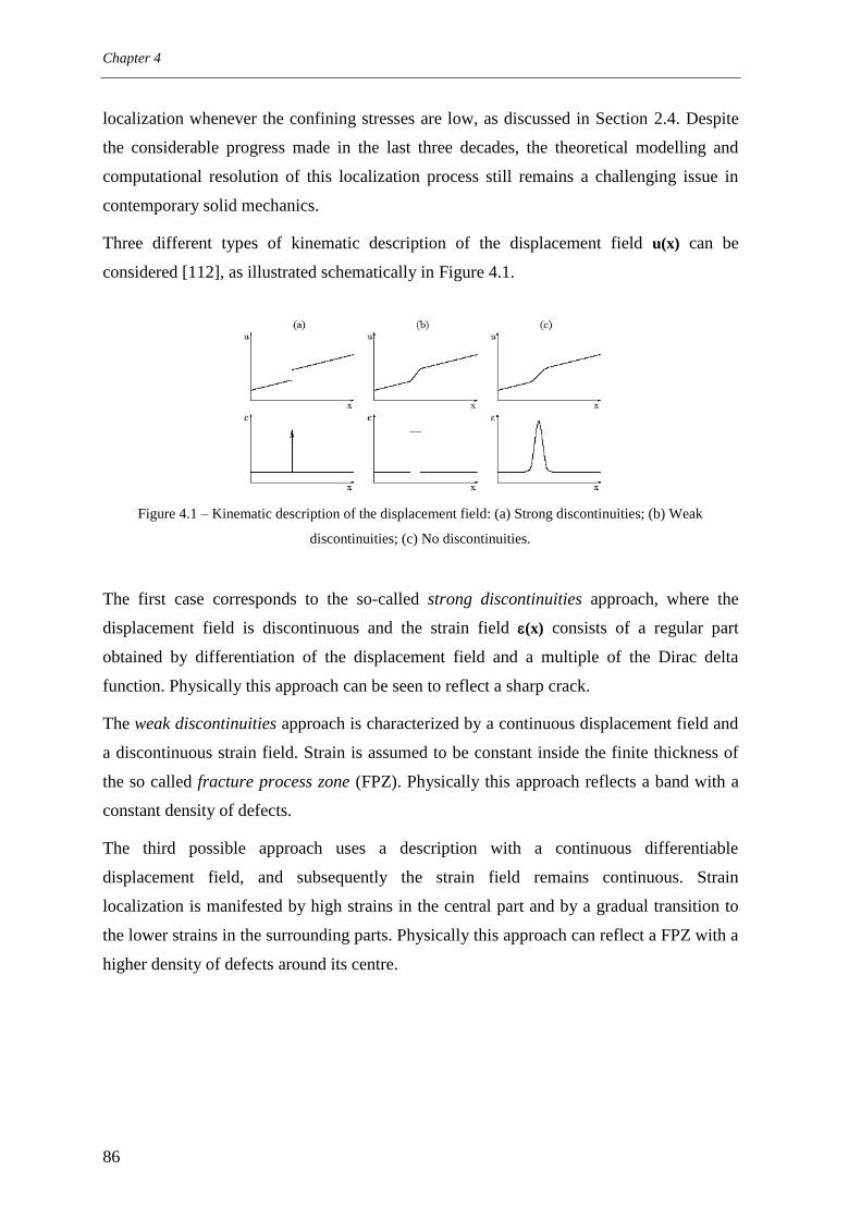
Chapter 4

86

localization whenever the confining stresses are low, as discussed in Section 2.4. Despite

the considerable progress made in the last three decades, the theoretical modelling and

computational resolution of this localization process still remains a challenging issue in

contemporary solid mechanics.

Three different types of kinematic description of the displacement field u(x) can be

considered [112], as illustrated schematically in Figure 4.1.

Figure 4.1 – Kinematic description of the displacement field: (a) Strong discontinuities; (b) Weak

discontinuities; (c) No discontinuities.

The first case corresponds to the so-called strong discontinuities approach, where the

displacement field is discontinuous and the strain field (x) consists of a regular part

obtained by differentiation of the displacement field and a multiple of the Dirac delta

function. Physically this approach can be seen to reflect a sharp crack.

The weak discontinuities approach is characterized by a continuous displacement field and

a discontinuous strain field. Strain is assumed to be constant inside the finite thickness of

the so called fracture process zone (FPZ). Physically this approach reflects a band with a

constant density of defects.

The third possible approach uses a description with a continuous differentiable

displacement field, and subsequently the strain field remains continuous. Strain

localization is manifested by high strains in the central part and by a gradual transition to

the lower strains in the surrounding parts. Physically this approach can reflect a FPZ with a

higher density of defects around its centre.

Implementation in a finite element code

87

4.2.2 Constitutive models and constitutive laws

4.2.2.1 Types of constitutive models

A constitutive model can be thought as the mathematical description of the material

behaviour which yields the relation between the stress and strain tensors in a material point

x of the body as a function of time t. The most general formulation is to consider the stress

at point x to be a functional of the deformation history of all points of the body [29]. This

concept can be simplified if the stress is only influenced by the strain field in a

neighbourhood of the material point. Formulations of this type constitute the so-called non-

local constitutive models. Most macroscopic constitutive models used in concrete

structures come into the class of local homogenous constitutive models, for which the

stress tensor depends only on the local strain tensor, and for which the material properties

do not depend upon the material point. Although an exhaustive classification of this

particular type of constitutive models is out of scope of the present thesis, for which the

reader is referred to [58; 254], a distinction is made between rate and total formulations. In

a constitutive model of the rate type the stress tensor at time t 1 is generically expressed by:

dtt

0, σxσ (4.1)

where the stress rate σ is generally given as a function of the strain rate ε and some

internal (state) variables κ , which keep track of the loading history:

κεxσ ,, ft (4.2)

Material models which comply with this description are, for instance, the ones based on the

flow theory of plasticity. In this particular case the stress rate is given by

peee εεDεDσ , where De is the fourth order elasticity tensor. The inelastic strain

rate κεεε ,pp can be considered a function of the total strain rate ε and of the vector

of state variables κ .

In the constitutive models following a total formulation, the stress vector is directly

computed from the total strain vector and can be most generally described by:

1 In this work, the variable time attains the role of a parameter which merely orders the loading process.

Although time-dependent effects are not going to be considered, a division of the loading process in a finite

number of increments is required. This will be referred to as a temporal discretization.

Chapter 4

88

κεxσ ,, ft (4.3)

Among others, secant pseudo-elastic models and models based on the theory of continuum

damage belong to this type of formulations. In these cases the stress tensor is given by

εDσ sec , where Dsec is a fourth-order secant stiffness tensor. In the particular case of

continuum scalar damage models this tensor can be expressed as Dsec = (1 – d) De, being d

the scalar damage variable(s) which keeps track of the previous loading history.

It must be realized that concrete is neither a plastic nor continuum damage like material. In

computational modelling of concrete structures, plastic flow or continuum damage theories,

to cite these two, are used to circumvent the lack of a realistic model for concrete and its

interaction with the reinforcement. The choice between several constitutive models is often

dictated by the availability of well established and sound numerical algorithms which

allow obtaining converged solutions beyond the failure load and which guarantee the

satisfaction of the basic thermodynamic requirements ensuring that meaningful structural

responses can be obtained in complex loading scenarios. However, in simpler cases, such

as the ones corresponding to plane stress conditions, sufficient experimental evidence on

the behaviour of RC elements is available sustaining the direct implementation of

phenomenological models such as the one developed in Chapter 3. As the number of

possible stress trajectories is smaller than in the general three-dimensional case, the model

can be validated for almost all the possible stress states, thereby eliminating the need for a

sound theoretical background. The phenomenological approach is followed in the work

presented in this chapter and the constitutive model is developed following a total

formulation as expressed by Eq. (4.3).

4.2.2.2 Constitutive laws, control volume and kinematic description of the

displacement field

A constitutive law (or relationship) is defined as the analytical expression relating two

individual components of the stress and strain tensors. The constitutive laws are the core of

a constitutive model and must be defined not only in close relation with the kinematic

description of the displacement field but also with the control volume over which they are

established. Regarding the latter, the work developed in the previous chapter represents an

illustrative example. Spatially averaged relationships were developed for reproducing the

behaviour of an array of cracks as a whole, thus efficiently reproducing the response of RC

panels.


89

In some cases this spatially averaged approach may not be applicable and the behaviour of

each individual crack must be tracked, for which fracture mechanics concepts must be

applied. This being the case, the relation between the kinematic description of the

displacement field and the constitutive laws for concrete in tension is very clear and is

taken here as an illustrative example. Within the strong discontinuities approach, and in the

simplest case, the crack faces may be assumed as stress free and the remaining material as

elastic. This drives necessarily to a singularity in the stress field at the crack tip and the

crack propagation criteria is based on energy considerations and stress intensity factors,

according to the linear elastic fracture mechanics (LEFM) laws. This approach is rarely

applicable with sufficient accuracy to concrete, and it is only valid when the FPZ

dimensions are negligible compared with the structural size. In general, the size of the FPZ

must be accounted for and nonlinear fracture mechanics (NLFM) laws must be applied. In

the case of the strong discontinuities approach, the fictitious crack model of Hilleborg and

co-workers [99] is the suited NLFM model (see Section 2.1.2). In the case of displacement

fields with localization bands bounded by weak discontinuities, the constitutive laws must

be formulated within the crack-band model [17]. Instead of lumping all the inelastic effects

in a line, in the crack-band model they are assumed to be uniformly distributed along the

FPZ. In the case of continuous displacement and strain fields, the appropriate constitutive

laws must be formulated within the concepts of the non-local continuum mechanics [10; 14;

110; 182].

4.2.3 Discretization strategy

The finite element method is the most widely used numerical approach in the domain of

solid mechanics. In this context, the discretization strategy to be adopted is closely related

to the description of the displacement field. In the case of the strong discontinuities

approach the simplest way is to allow crack propagation through the boundaries of the

finite elements [2]. Also re-meshing techniques can be used [107]. If the crack pattern is

known in advance another approach is to use special interface elements with zero thickness

[77; 198]. More powerful approaches use a more elegant and efficient procedure using

finite elements enriched with terms that can reproduce jumps in the displacement field. For

an overview of the broad type of enriched formulations see [111; 112] and for comparative

analysis of their performance refer to [174].

Regular finite elements can be used with the other two kinematic descriptions of the

displacement field and corresponding constitutive laws. Within the weak discontinuities

Chapter 4

90

concept the localized strain is assumed to be smeared along a length, the crack-band width,

which must be somehow related to the size of the finite element in order to ensure the

correct energy dissipation. In the case of the non-local approach the strain distribution

within the FPZ can be obtained, requiring a high degree of mesh refinement and the use of

appropriate non-local constitutive models.

The discretization strategy must also be related to the type of constitutive law. If spatially

averaged constitutive laws are adopted for RC (such as the ones developed in Chapter 3)

the finite element size can be taken larger than the crack spacing. However, if constitutive

laws based exclusively upon fracture mechanics concepts are considered, a higher degree

of mesh refinement is required for tracking the propagation of each individual crack. Using

the crack band model and with proper mesh refinement, tension stiffening effects can be to

some extent approximated without explicitly taking into account bond slip effects, as

discussed by Cervenka [56].

4.2.4 Discussion

The strong discontinuity approach initiated by Simo et al. [220] and widely used over the

last years offers the possibility of merging continuous constitutive models for the bulk

response and a cohesive model for the discontinuous part of the kinematics in the same

formulation. This is certainly appealing from the physics of fracture point of view. Recent

developments [173] enabled successful applications of this type of approach to RC

problems exhibiting multiple cracks and concrete-reinforcement interaction [175].

However, as recognized by Oliver and Dias [172] these methods require a degree of

sophistication that seems to place a limitation on their incorporation in commercial

simulation codes and to their use in real scale civil engineering structures analyses. New

developments [172] are being attempted to overcome these difficulties.

Non-local models were formulated for dealing with situations where failure is governed by

the propagation of one or a few cracks. In these circumstances, the mesh induced

directional bias1 [199] and stress locking

2 [115; 197] exhibited by the classical local

constitutive models, which use a description of the displacement field based on weak

discontinuities, leads in some cases to poor estimates of the crack trajectories and of the

1 Mesh induced directional bias can be defined as the tendency for the localization regions to follow the

direction defined by the finite element sides. 2 Stress locking is referred to the spurious stress transfer between the two sides of a crack resulting from the

inability of the finite element interpolation to reproduce the discontinuous nature of the actual displacement

field.


91

post-peak branches of force-displacement curves. However, besides some known

shortcomings adhering to the nonlocal description of the continuum (see for instance [114;

221]), the use of very fine meshes and non-trivial parameters – in the sense that they

cannot be experimentally determined – are required in the formulation of the non-local

constitutive models, which still inhibits its practical application.

The models based on the concept of weak discontinuities are the most widespread in the

analysis of civil engineering structures, still presenting the best compromise between

accuracy, simplicity and economy of computer resources, and allowing the use of standard

finite element formulations. Not only localized cracking problems can be analysed with

sufficient accuracy for engineering purposes, see discussion by Cervenka [54], but also

distributed cracking patterns in the presence of bonded reinforcement can be treated within

the same framework. The use of spatially averaged constitutive laws allows the definition

of very effective relationships for the reinforced concrete material, thus constituting the

most efficient way for the analysis of large scale structural concrete elements. Therefore,

this was the approach followed in this work.

4.2.5 Solution procedures for nonlinear systems

4.2.5.1 Incremental – iterative solution of the equilibrium equations

From a mathematical point of view the determination of the continuum displacement field

u of a body in static equilibrium with external solicitations , constrained by a set of

boundary conditions and fulfilling the material constitutive laws, consists in the solution of

a boundary value problem (BVP) of the form:

φuL (4.4)

with L being a second order differential operator. As previously mentioned, the finite

element method is the most commonly used method to solve this BVP. This being the case,

static equilibrium can be most conveniently expressed in the integral (weak) form using the

principle of virtual displacements:

dSdVdV TTTtubuσε

(4.5)

Chapter 4

92

In the equation above, u is a kinematically admissible virtual displacement vector, is

the corresponding linearized1 virtual strain vector, is the internal stress vector, b are the

external forces applied to the body , and t are the tractions defined on the boundary ∂.

The left hand side of equation (4.5) represents the virtual work performed by the internal

forces which must be equal to the virtual work of the external forces given in the right

hand side.

In FEM the continuum is discretized in finite elements and the continuum displacement

and strain fields are recovered from the vector of nodal displacements, a, using the

interpolation matrix N, and the deformation matrix B, respectively:

aNu aBε (4.6)

Considering that the equality (4.5) must be fulfilled for every virtual displacement field,

and taking into account (4.6) it can be shown [176] that in the context of FEM static

equilibrium can be alternatively expressed by:

0fp (4.7)

with the internal forces given by:

dVTσBp (4.8)

and the external forces by:

qNtNbNf

TTT dSdV (4.9)

with q being the vector of point forces.

For problems governed by a nonlinear differential operator L, the internal force vector p is

a nonlinear function of the nodal displacements a and the solution to equation (4.7) can be

found using an incremental-iterative procedure. The incremental nature of the solution

procedure is reflected by the stepwise loading application, which can be thought as a

discretization in the time domain. At a given stage t+t, the system of equilibrium

equations to be solved reads:

0aψfap tttttt 0 (4.10)

1 Small deformations are assumed throughout this section


93

where ψaψ is the vector of the unbalanced forces (or residuals), which must vanish

within a prescribed accuracy, is a scalar load factor and f0 the reference external force

vector. The equilibrium solution from the previous load stage t

taa 0ff t 0ψ t (4.11)

is altered when the next load step 0ftt is applied,

0fff ttttt (4.12)

The Newton-Raphson method, which will be used throughout this thesis, can be derived

performing the linearization of (4.10) in a neighbourhood of the current state:

0aa

ψψψ

11 i

att

i

tt

i

tt

i

tt (4.13)

The equation above is solved iteratively, see Figure 4.2. The superscript i is the iteration

counter and

i

tt

i

tt

i

tt

K

a

p

a

ψ (4.14)

where K is the assembled (or structural) tangential stiffness matrix. The iterative update to

the nodal displacement vector is readily obtained from (4.13):

i

tt

i

tt

i

tt

ψKa11 (4.15)

After a series of iterations the incremental nodal displacement vector is given by:

1

1

1i

k

k

tt

i

tt aa (4.16)

In the context of FEM, the structural tangential stiffness matrix is obtained from

dVi

tt

Ti

tt BDBK

(4.17)

where the matrix

Chapter 4

94

i

tt

i

tt

ε

σD (4.18)

is the constitutive tangent stiffness matrix, which is evaluated at each integration point

using the appropriate constitutive model.

Figure 4.2 – Newton – Raphson iteration. Notation.

4.2.5.2 Line-search technique

The Newton-Raphson method is shown not to be globally convergent. The method is based

on reasonable predictions of the iterative correction to the nodal displacement vector such

that the iteration process converges to an equilibrium solution. However, the iterative

predictions may sometimes be too far from the equilibrium path and convergence cannot

be found. This can happen in processes with strong nonlinearities, such as cracking or

constitutive laws involving softening (see Section 4.2.5.5), which is usually the case in

concrete structures. In these circumstances, line search algorithms can significantly

enhance the robustness of the Newton-Raphson method.

In the line search technique, the search direction at a given iteration is defined by the

iterative update of the nodal displacement vector 1

i

tta . The updated displacement vector

is now written as

1,,1

i

tt

jii

tt

ji

tt aaa (4.19)


95

where the superscript j is the counter of line searches, and is the line search factor which

scales the iterative update to the displacement field in order to bring it closer to the

equilibrium path. The scalar is determined such that the projection of the residuals in the

search direction is smaller than a predefined tolerance by solving the scalar inequality

i

tt

Ti

tt

i

tt

jii

tt

Ti

tt

aψaaaψa11,1 (4.20)

through a local iterative method. The tolerance that was used in the examples presented in

this thesis is defined by setting the scalar = 0.8, which is the default value implemented

in DIANA and was found to be sufficient to stabilize the global iteration process. For

details and more references regarding this technique refer to [70; 76; 135; 256].

4.2.5.3 Constrained Newton-Raphson

With the standard load control method described above, in which the incremental load

factor tt is kept constant during the equilibrium iterations, the softening branch of the

structural response cannot be obtained. Moreover, this method also fails at local peaks of

the force-deformation curve. This deficiency can be overcome by using the arc-length

method [69]. This method adds a new constraint equation to the system of nonlinear

equations given by (4.10), which considers tt as an additional variable,

0, ttttf a (4.21)

thus introducing the possibility of overcoming local limit points by iterating in the load-

displacement space. In this work, the update normal plane constraint [191] was adopted,

0aa

1i

tt

Ti

tt (4.22)

which sets an orthogonality condition between the incremental and the iterative update

nodal displacement vectors. In order to determine the incremental load factor from the

equation above, the iterative update to the nodal displacement vector is split in two parts:

111

0

111

0

11

11

i

tt

IIi

tt

i

tt

I

i

tt

i

tt

i

ttt

i

tt

i

ttt

i

tt

i

tt

i

tt

i

tt

i

tt

aa

fKpfK

ffpK

ψKa

(4.23)

Chapter 4

96

The first part, 1

i

tt

Ia , is obtained from the difference between the external forces at the end

of the last converged load step and the internal forces after iteration i. The second part,

11

i

tt

IIi

tt a , is related to the external load increment being applied in the current load

step. After substitution of Eq. (4.23)4 into the constraint equation (4.22), the incremental

load factor is determined:

1

11

i

tt

IITi

tt

i

tt

ITi

tti

tt

aa

aa

(4.24)

In cases of strong localization of deformations leading to very brittle responses, it can be

more efficient to use a reduced set of active degrees of freedom in the nodal displacement

vector. In these circumstances, the vectors a and a used in the constraint equation (4.22)

are obtained from a modified displacement vector defined as

0.......0 paa (4.25)

with pa being a subset of a . In the extreme situation where only one degree of freedom is

chosen to be active, this method is also called indirect displacement control. The active

degrees of freedom must be selected with engineering judgement. In this work, this

procedure is only adopted when the regular arc-length control method fails. For a more

complete description and more references concerning the arc-length method refer to [29;

76; 135; 256].

4.2.5.4 Convergence criterion

The Newton-Raphson iterative process described above is stopped when the solution is

sufficiently close to the equilibrium path, in which case a convergence criterion established

using an appropriate metrics is fulfilled. In this thesis, the metrics based on the so called

energy norm [256]

tolE

E

tttt

T

tt

i

tt

i

tt

Ti

tt

tt

i

tt

010

11

0ppa

ppa

(4.26)

was adopted, see Figure 4.2. This norm is more versatile than the usual Euclidean norm of

the out-of-balance force vector, especially in the cases where the structural response


97

exhibits a yielding plateau. The convergence criterion was defined by setting the tolerance

tol = 10-4

.

4.2.5.5 Some comments on the uniqueness of the solution

According to the definition first presented by Hadamard [93], a BVP is said to be well-

posed if: (1) a solution exists; (2) the solution is unique; and (3) the solution depends

continuously on the data. Mathematically, the ellipticity of the differential operator L is a

necessary condition for the desired property of well-posedness of a BVP in the form of Eq.

(4.4). In the context of finite element analyses, the existence of a unique solution for the

problem at hand and the fact that the solution does not involve discontinuities practically

ensures a smooth convergence of the numerical iterative methods and the independence of

the solution with respect to the adopted finite element mesh, i.e., mesh objectivity of the

results.

Considering the adopted incremental solution procedure, equilibrium at the infinitesimal

scale can be re-written in rate form as:

εDσ (4.27)

where D is the tangent constitutive stiffness matrix as defined in Eq. (4.18). It can be

shown [35; 116; 254] that loss of ellipticity of the local BVP occurs when there is a

normal unit vector n such that:

0det DnnT (4.28)

which also defines the necessary condition for the onset of localization of deformations

along the surface defined by n [113; 116; 254]. In constitutive models involving softening

or perfectly plastic behaviour, condition (4.28) is satisfied at the onset of the softening or

yielding regimes, respectively. In these circumstances, deformations tend to localize in

narrow regions of the structure, in spite of the fact that the external actions continue to

follow a monotonic loading programme. This effect is more severe in constitutive models

exhibiting softening. According to what was stated above, if there is a vector n that

satisfies Eq. (4.28), the solution ceases to be unique. In these circumstances, it is not

guaranteed that the solution found through the above described nonlinear solution

Chapter 4

98

procedures is the one corresponding to the global minimum of the system elastic potential

energy. As mentioned in Section 4.2.4 the solutions may also be strongly dependent on the

adopted finite element mesh, which is an inherent shortcoming of the traditional local

constitutive models based on the concept of weak discontinuites. Objectivity of the results

with respect to the size of the finite elements can be achieved by introducing the

localization band length into the constitutive laws, as in the crack band model. However,

mesh induced directional bias cannot be as easily removed. Non-local constitutive models

are shown to restore the well-posedness of the local BVP. Another way of circumventing

the problem is to perform a bifurcation analysis using the localization tensor DnnT , and

adding a deformation mode affine with the lowest (negative) eigenvalue. This procedure is

described in detail in reference [29] and constitutes the basis of the modern strong

discontinuity approaches. For a detailed discussion on this topic refer to references [29;

254].

4.3 Total strain based model

The total strain smeared crack model developed within this work is implemented in the

user supplied subroutine USRMAT in the finite element code DIANA. A set of state

variables continuously monitor the damage evolution in concrete and enable establishing

suitable loading/unloading/reloading conditions. The flowchart of the subroutine is

presented in Figure 4.3. The objective is to determine the updated vector of the internal

stresses, to update the state variables vector k and to determine the tangent constitutive

matrix D in each iteration of the incremental-iterative procedure. The remaining operations

described in Section 4.2.5 are performed by DIANA.


99

IDCRK = 0 ?IDCRK = 0 ?Call

CONC2D

Yes

Call

PRINC

Call

CRKCRI

IDCRK = 0

?

Set and transfer

internal variables

Yes

Call

TRANSF

No

Call

CONC1D (-t)

Call

CRKSHE

Call

CONC1D (-n)

Assemble the

concrete stress

vector in the crack

coordinate system

Call

TRANSF

Assemble the concrete

iteration stiffness matrix

in the crack coordinate

system

Call

GBLMAT

No

Call

REINF

Assemble the

composite stress

vector in the element

coordinate system

Assemble the composite

iteration stiffness matrix

in the element

coordinate system

RETURN

Read and check

input data

START

Call

UPDATE

Get data from the

state variables

vector

(*)

(**)

Figure 4.3 – Flow chart of the subroutine.

The relevant input data consists of the user defined model parameters, the total strain

vector in the last converged load step, the current incremental strain, the vector of the state

variables, and the current stress vector. After reading and checking the input data, the state

variables values are assigned to a set of internal variables, which are used and modified

throughout the subroutine. The indicator IDCRK monitors the cracking condition: IDCRK

= 1 or = 0 whether cracking has or not occurred in the past history, respectively. If concrete

is uncracked, the CONC2D subroutine is invoked for calculation of the concrete stresses

and concrete iteration stiffness matrix. The concrete principal stresses and the principal

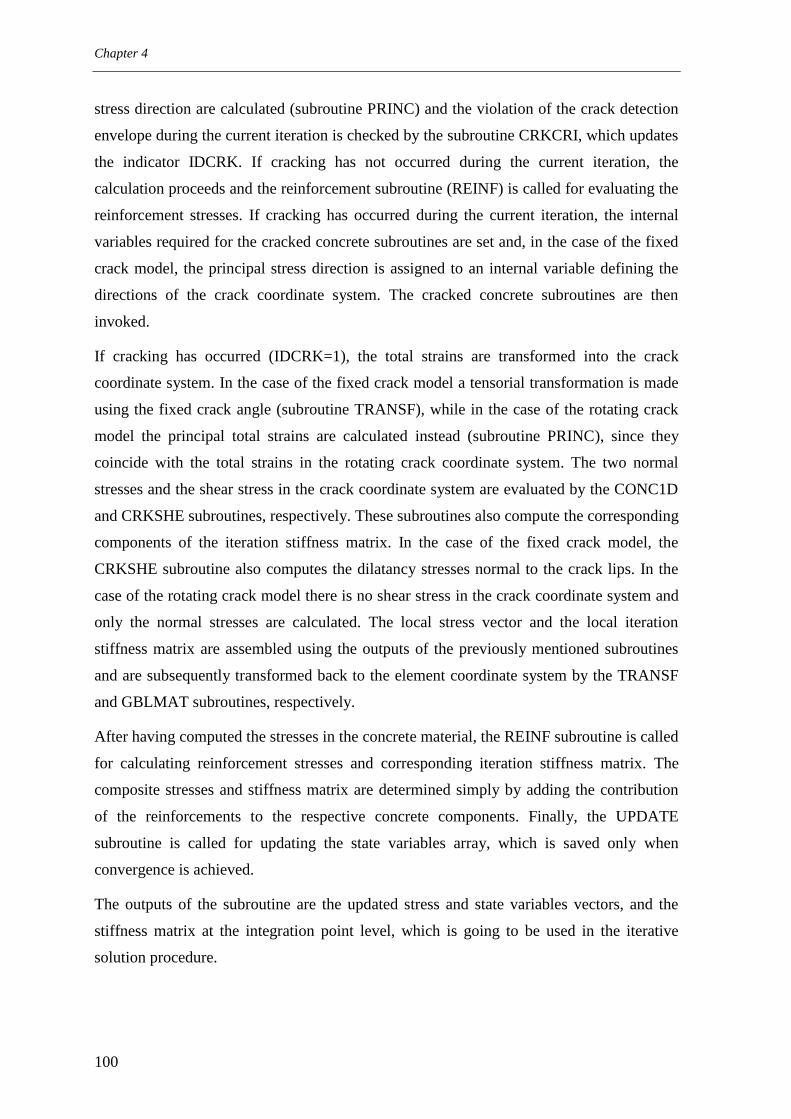
Chapter 4

100

stress direction are calculated (subroutine PRINC) and the violation of the crack detection

envelope during the current iteration is checked by the subroutine CRKCRI, which updates

the indicator IDCRK. If cracking has not occurred during the current iteration, the

calculation proceeds and the reinforcement subroutine (REINF) is called for evaluating the

reinforcement stresses. If cracking has occurred during the current iteration, the internal

variables required for the cracked concrete subroutines are set and, in the case of the fixed

crack model, the principal stress direction is assigned to an internal variable defining the

directions of the crack coordinate system. The cracked concrete subroutines are then

invoked.

If cracking has occurred (IDCRK=1), the total strains are transformed into the crack

coordinate system. In the case of the fixed crack model a tensorial transformation is made

using the fixed crack angle (subroutine TRANSF), while in the case of the rotating crack

model the principal total strains are calculated instead (subroutine PRINC), since they

coincide with the total strains in the rotating crack coordinate system. The two normal

stresses and the shear stress in the crack coordinate system are evaluated by the CONC1D

and CRKSHE subroutines, respectively. These subroutines also compute the corresponding

components of the iteration stiffness matrix. In the case of the fixed crack model, the

CRKSHE subroutine also computes the dilatancy stresses normal to the crack lips. In the

case of the rotating crack model there is no shear stress in the crack coordinate system and

only the normal stresses are calculated. The local stress vector and the local iteration

stiffness matrix are assembled using the outputs of the previously mentioned subroutines

and are subsequently transformed back to the element coordinate system by the TRANSF

and GBLMAT subroutines, respectively.

After having computed the stresses in the concrete material, the REINF subroutine is called

for calculating reinforcement stresses and corresponding iteration stiffness matrix. The

composite stresses and stiffness matrix are determined simply by adding the contribution

of the reinforcements to the respective concrete components. Finally, the UPDATE

subroutine is called for updating the state variables array, which is saved only when

convergence is achieved.

The outputs of the subroutine are the updated stress and state variables vectors, and the

stiffness matrix at the integration point level, which is going to be used in the iterative

solution procedure.


101

4.3.1 Uncracked concrete

In this section, the theory and the algorithm behind the CONC2D subroutine are described.

For uncracked concrete, an efficient isotropic damage like formulation is adopted,

requiring only one state variable for tracing the damage evolution and establishing the

loading/unloading/reloading conditions.

4.3.1.1 Equivalent stress

The equivalent stress S is here defined as a scalar measure of the applied stress level under

biaxial plane stress conditions. For S = 0 concrete is totally unloaded while for S = 1 the

biaxial failure envelope has been reached. As proposed by Maekawa [136], the equivalent

stress can be defined as a function of the two invariants of the stress tensor,

22

d

c

m

c f

b

f

aS

61.0a

27.1b

(4.29)

with m and d being, respectively, its mean and deviatoric invariant components:

212

2 m

212

2 d , 21

(4.30)

The two parameters a and b in Eq. (4.29) were determined from experimental data for the

uniaxial compression and equal biaxial compression stress trajectories. In these cases the

principal stresses at failure are given by cf :0: 21 and cc ff 16.1:16.1: 21 ,

respectively. In Figure 4.4 the resulting failure envelope (S=1) is presented in the 1 - 2

plane and it is compared to the Kupfer and Gerstle [128] failure criteria, which was

adopted by the CEB in the Model Code 1990 [40]. The crack detection envelope

represented in the figure is used for detecting if cracking has occurred. When this envelope

is violated, the cracked concrete subroutines are invoked.

Chapter 4

102

Kupfer and Gerstle

Present criteria: S=1

Crack detectionsurface

1 / f c '

2 / f c ' -0.52:-1

-1:-1

-1:-0.52

0.0

0.5

1.0

1.5

0.0 0.5 1.0 1.5

Figure 4.4 – Proposed failure criterion in the σ1- σ2 stress plane.

4.3.1.2 Equivalent total strain

The equivalent total strain E is a scalar measure of the current biaxial total strain level.

Similar to the equivalent stress, for E=0 concrete is unloaded while for E=1 the failure

envelope is reached. The equivalent total strain is also defined as a function of the two

invariants of the total strain tensor [136],

2

0

2

0

dm

dcE

62.0c

10.1d

(4.31)

with m and d being, respectively, its mean and deviatoric invariant components:

212

2 m

212

2 d , 21

(4.32)

The two parameters c and d in Eq. (4.31) were derived such as to fit the peak strains

obtained in the uniaxial compression and equal biaxial compression tests.

4.3.1.3 Stress-strain relationships and loading/unloading determination

In a monotonic loading process it is assumed that the equivalent stress S can be univocally

obtained from the equivalent total strain E through the following nonlinear relationship:


103

1,

212

1

1

1,21

2

2

E

EE

EEk

EEk

S

(4.33)

For the ascending branch, 1E , the Sargin‘s law was adopted [84], while for the

descending (post-peak) branch a modified version of the function proposed by Krätzig and

Pölling [125] was defined, ensuring a smooth transition between the two branches. The

parameter k determines the shape of the curve in the ascending branch. With k=2, a

parabolic relationship is obtained. In general,

0

c

ci

f

Ek (4.34)

with ciE being the initial tangential modulus of elasticity in a uniaxial compressive test. The

parameter controls the shape of the curve in the descending branch. The post-peak

response must be regularized according to the dimension of the strain localization band, hC,

which is related to the finite element size. It is proposed to use

2

0

0

22

1

cCC

c

fhG

f (4.35)

where GC is the compressive fracture energy. Unless stated otherwise, GC is estimated

using the Compressive Damage Zone (CDZ) model proposed by Markeset and Hillerborg

[144] considering k = 3, r = 1.25 mm, wc = 0.6 mm and L = 2.5∙e, being e the element

thickness:

cFC feGG 0003.01500 (4.36)

In Figure 4.5, the resulting uniaxial stress-strain curves for an element with

length/width/thickness of 0.25x0.25x0.10m3 are presented for 5 different uniaxial concrete

strengths. The fracture energy GF, the Young modulus Eci and the peak uniaxial

strain 0 were calculated according to the equations given in Chapters 2 and 3.

Chapter 4

104

0

1

0 3

S

E

f ' c = 20

40

60 (Mpa)

80

100

0

100

0 0.006

- 2

- 2

Figure 4.5 – Graphical representation of the proposed stress-strain curve in the uniaxial compression case

for 5 different concrete strengths: (a) Equivalent stress vs. equivalent strain; (b) Resulting uniaxial stress-

strain curves.

In the present model, a loading step always leads to damage evolution while in an

unloading/reloading step damage remains constant. The variable that is used to monitor

damage evolution is the maximum equivalent total strain, Emax, which by definition is a

non-decreasing variable. A given Emax value bounds a region in the total strain space where

no damage evolution occurs – the reversible process domain. This region expands as the

maximum total strain increases and can never contract.

The implemented algorithm is given in Box 4.1. A value of r < 1 corresponds to an

unloading or to a reloading step, while r = 1 corresponds to a loading step.

Box 4.1 – Algorithm for loading/unloading determination and calculation of the current equivalent stress.

1 – Calculate the current equivalent total strain ttE from the current total strain

tensor tt ε

tttt fE ε Eq. (4.31)

2 – Calculate the current maximum equivalent total ttE

max strain and the strain ratio r.

ttttt EEE ,max maxmax % State variable

tt

tt

E

Er

max

3 – Calculate the equivalent stress corresponding to ttE

max .

tttt EfS maxmax Eq. (4.33)

4 – Calculate the current equivalent stress ttS

tttt SrS max


105

4.3.1.4 Constitutive and iteration stiffness matrices

So far, only a scalar relationship between the equivalent stress and equivalent total strain

was defined. To complete the formulation, a directional relationship between the total

strain and stress tensors is required. In the present model, before cracking, concrete is

treated as an isotropic material. At higher loading levels this is a simplifying assumption,

as shown in reference [136]. Nonetheless, it greatly simplifies the model while the error

that is introduced is small and has little significance on the overall response of a RC

member under biaxial stress conditions. The secant constitutive matrix relating concrete

stresses with the total strains is derived in the form of a nonlinear elasticity matrix

xy

y

x

c

cxy

cy

cxE

2

100

01

01

1 2

sec,

220

sec,

11

d

c

m

c

cc

f

b

f

a

SfE

(4.37)

where Ec,sec is the secant Young modulus and is the Poisson ratio for which a constant

value = 0.2 may be taken. The expression for Ec,sec is directly obtained from the

definitions of equivalent stress and equivalent strain given by Eqs. (4.29) and (4.31),

respectively.

The secant stiffness matrix of Eq. (4.37) is used to calculate stresses for the given strain

state. The tangent stiffness matrix Dc is used for construction of an element stiffness matrix

for the iterative solution at the structural level. This matrix can readily be obtained in the

global coordinate system replacing Ec,sec in Eq. (4.37)1 by the tangential modulus Ec,tan,

which is the slope of the equivalent stress-strain curve at a given total strain:

MIN

c

MIN

cc

c

E

EEk

EkEkf

E

tan,

tan,2

2

0tan,21

)2(2

1,

1,

E

E (4.38)

The tangent modulus as defined in Eq. (4.38) is always positive. Whenever the slope of the

curve is less than the minimumMIN

cE tan, the value of the tangent modulus is set to

Chapter 4

106

MIN

cc EE tan,tan, . This occurs in the softening range and near the compressive peak. Strictly

speaking, in these situations the stiffness matrix ceases to be tangent.

The resulting algorithm is simple and is given in Box 4.2. Both the stresses and tangent

stiffness matrix are determined explicitly from total strains.

Box 4.2 – Algorithm for computation of the stresses and tangent stiffness matrix

1 – Calculate the current equivalent total strain ttE and the current equivalent stress ttS using the algorithm in Box 4.1.

2 – Calculate the current value of the secant modulus tt

cE

sec,

tttttt

c SfE ,sec, ε Eq. (4.37)2

3 – Calculate the concrete stresses from the total strains using Eq. (4.37)1

4 – Calculate the current value of the tangent modulus tt

cE

tan,

IF r = 1 % Loading step

tttttt

c SEfE ,tan, Eq. (4.38)

ELSE % Unloading/reloading step

MIN

c

tt

c

tt

c EEE tan,sec,tan,

END

5 – Assemble the stiffness matrix Dc directly in the global coordinate system using tt

cE

tan,

in Eq. (4.37)1

4.3.1.5 Examples

Biaxial compression - comparison with the experimental results of Kupfer and Gerstle

In Figure 4.6 the results from the analytical model are compared to a classical set of

experimental data [128] with three compressive biaxial stress trajectories (see also Figure

4.4). The agreement is quite good in view of the simplifications considered in the model,

such as the isotropy assumption and the constant value for the Poisson coefficient.


107

0.0

0.5

1.0

1.5

-1.0 0.0 1.0 2.0

- 2 / f c '

- 1 / 0' - 2 / 0'

-0.52/-1

-1:-1

1: 2 = 0:-1

Figure 4.6 – Comparison of analytical model (k=2.375, =0.2) with experimental data from reference

[128].

Loading/unloading/reloading tests

In Figure 4.7 the model response for the case of non-proportional loading under biaxial

compression stress states is presented. In a first stage, a uniaxial compression loading was

applied till the equivalent stress reached S = 0.7, after which followed an unloading stage.

Then a biaxial compression loading path was applied following the stress trajectory

1:2 = -0.52:-1 till the equivalent stress reached S = 0.85. After unloading, a biaxial

compression loading path was finally applied following the stress trajectory 1:2 = -1:-1.

The stress trajectories are represented in Figure 4.7 (a) and the corresponding strain

trajectories in Figure 4.7 (b). Due to the adoption of a constant Poisson ratio, the strain

trajectories are straight lines. A given value of the maximum equivalent strain bounds the

domain of reversible stress states, as discussed in Section 4.3.1.3. In Figure 4.7 (c) the

equivalent stress-equivalent strain relationship is depicted. The

loading/unloading/reloading behaviour of the model can be clearly perceived. The points

corresponding to the boundary of the reversible process at the end of each loading stage are

represented by symbols. The normalized principal stress-principal strain curves are shown

in Figure 4.7 (d). The points corresponding to the boundary of the reversible process are

represented by the same symbols as in Figure 4.7 (c). It can be seen that the

unloading/reloading portions of the stress-strain curves are straight lines, corresponding to

stress and strain trajectories inside the boundaries delimiting the reversible process.

Chapter 4

108

1 / f c '

2 / f c ' -0.52:-1

1: 2=-1:-10:-1

0.0

0.5

1.0

1.5

0.0 0.5 1.0 1.5

0.7

0.85

S=1.0

1 / 0 '

2 / 0 '

0.0

0.5

1.0

1.5

0.0 0.5 1.0 1.5

0.411

0.568

E=1.0

(a) (b)

0.0

0.5

1.0

0.0 0.5 1.0 1.5

S

E

E = 0.411

S = 0.7

E = 0.568

S = 0.85

0.0

0.5

1.0

1.5

- 2 / f c '

- 1 / 0' ; - 2 / 0'

2: 2

2: 1

0.0 0.5 1.0 1.5

(c) (d)

Figure 4.7 – Model behaviour under non-proportional biaxial compression loading paths: (a) Load paths in

the principal stress space and (b) corresponding principal strain trajectories; (c) equivalent stress-

equivalent strain relationship; (d) minimum compressive stress ratio versus the two principal strain ratios.

4.3.2 Cracked concrete

After cracking, concrete is treated as an orthotropic material and a local coordinate system

is introduced (n-t coordinates) where the constitutive laws are established. The total strains

in the global coordinate system are transformed into the local coordinate system through

the usual strain transformation relationship:

ntε = T hvε

hv

v

h

nt

t

n

sccscs

cscs

cssc

22

22

22

22

,

cos

sin

c

s (4.39)


109

where the subscripts (∙)h and (∙)v refer to the horizontal and vertical axis of the global

coordinate system, respectively, and is the angle between the h-axis and the normal to the

cracks.

Once cracking occurs, two uniaxial stress fields are assumed along the two orthogonal n-t

directions and the Poisson effect in the cracked concrete is neglected. In the case of

rotating crack models, the local coordinate system rotates and the n-direction is aligned

with the direction of the maximum principal total strain, i.e., =. In the case of fixed

crack models, the crack direction is determined by the principal tensile direction of the

concrete stress tensor at impending cracking. The crack angle remains fixed and is kept

in memory as a state variable.

4.3.2.1 Compression model parallel to crack direction

The compressive stress parallel to the crack direction is determined from the total strain

along the respective local axis using the base curve (4.33) already adopted in the uncracked

stage. However, as the compressive strength of cracked concrete is reduced with increasing

tensile strains in the orthogonal direction , the compressive strength cf must be replaced

by the effective compressive strength cefefc ff , . In the case of the fixed crack model,

the peak uniaxial strain is also reduced to 0,0 efef . Both the equivalent stress and the

equivalent strain of cracked concrete are calculated according to Eqs. (3.27). It is remarked

that instead of using the current tensile strain , the maximum tensile strain in the past

history max, is used for computing the softening coefficient e .

max,8108.1

1

m

eC

(4.40)

This is required in order to ensure thermodynamic consistency, i.e., that energy cannot be

generated during an arbitratry loading/unloading/reloading cycle.

In the case of cracked concrete, the parameter cr replaces in Eq. (4.33)2 and controls

the shape of the compression curve in the post-peak branch, being calculated by:

2

0

,0

2

,

ef

c

efc

crf

f (4.41)

Chapter 4

110

4.3.2.2 Tension model normal to crack direction

Depending on the material model formulation, the tension model can either relate the crack

bridging stresses with the smeared crack opening, being in this case a tension softening

model, or the average concrete tensile stresses in the reinforced concrete domain with the

average strains, i.e., a tension stiffening model. In the present formulation, the material

model relates the stresses at the cracks with the average strains and, therefore, only a

tension softening formulation is included. The selected crack bridging stress law is the one

described in Section 3.6.2.

In the case of plain concrete, tensile fracture is a localized phenomenon and some kind of

regularization of the strain field must be employed. As previously discussed, the crack

band model is considered here and, therefore, the crack opening w and the total tensile

strain are related by

thw (4.42)

with ht being the crack band width, which is a function of the finite element size and type,

integration rule and crack orientation. A correct definition of the crack band width is very

important in the case of unreinforced or poorly reinforced structures in order to ensure the

correct amount of energy dissipation during the fracture process. The propagation of a

vertical crack parallel to the element sides and an inclined crack is schematically depicted

in Figure 4.8.

In the case of linear quadrilateral elements, and if the crack propagates parallel to the sides

of the finite elements, the crack band width equals the size of the element side. However, if

the crack propagates diagonally, the crack band width can be larger than the projection of

the element side along the normal to the cracks due to the fact that cracks also occur in the

neighbouring elements. This introduces an orientation effect in the calculation of the crack

band width. In the present implementation this effect is taken into account following the

proposal of Cervenka et al [57] by increasing the crack band width according to Eq.(4.43),

in which h is the projection of the finite element dimensions along the normal to the cracks

and ht is the corrected crack band width. According to Eq. (4.43), it can be easily seen

that hht 5.10 .


111

21

hht , 4;0 (4.43)

If quadratic finite elements are used instead, cracks may localize on some of the integration

points. In the case of a 2x2 reduced integration scheme, the propagation of both vertical

and diagonal cracks is schematically depicted in Figure 4.8 (c) and (d), respectively. In this

case, h is the projection of the gauss point tributary length along the normal to the cracks.

(a) (b)

(c) (d)

Figure 4.8 – Calculation of the crack band width: (a) propagation of a vertical crack in linear quadrilateral

elements; (b) propagation of an inclined crack in linear quadrilateral elements; (c) propagation of a vertical

crack in quadratic quadrilateral elements; (d) propagation of an inclined crack in quadratic quadrilateral

elements.

Chapter 4

112

4.3.2.3 Coupled tension-compression model

The combination of the compression and tension models results in a path-dependent model,

which is required in case of non-proportional or reversed loading paths. Note that, even in

the case of proportional monotonic loading, stress redistributions within the structure may

lead some regions to unload. The unloading/reloading is performed secant to the origin.

For reproducing this type of behaviour two state variables are required for each direction of

the local coordinate system: the maximum and minimum total strain experienced in the

past history. In the present implementation, instead of the minimum compressive strain, the

state variable governing the compressive behaviour is the maximum equivalent total strain

in the past history. Immediately after cracking, the state variable tEmax from the uncracked

subroutines is transferred to the cracked subroutines:

tt

t

t

n EEE maxmax,max, (4.44)

which is equivalent to assuming an isotropic damage evolution prior to cracking.

The loading/unloading determination is made independently for the n- and t-directions

according to the algorithm described in Box 4.3. Similarly to the uncracked concrete

subroutines, a value of r < 1 corresponds to an unloading or to a reloading step while r = 1

corresponds to a loading step. Once concrete is cracked, the biaxial confinement effects

cannot be recovered.


113

Box 4.3 – Algorithm for loading/unloading determination and current normal stress calculation (cracked state)

1 – Transform the total strains from the global to the local coordinate system.

tt

nt

ε = T tt

hv

ε Eq.(4.39)

Note that is either a state variable, in the case of fixed crack models, or is

calculated from the current total strain tensor, in the case of rotating crack models. In this

last case the notation tt should have been used.

2 – Calculate the current normal stress tt

n

in the n-direction:

i. Evaluate the softening coefficient ef :

tt

t

t

t

tt

t

,max max,max, % State variable

IF 0max, tt

t

tt

t

max, with f and e given by Eqs.(3.24).

ELSE

1ef

END

ii. For compressive stress states, 0 tt

n

ef

tt

ntt

nE,0

, with 0,0 efef in the case of the fixed crack model

tt

n

t

n

tt

n EEE ,max max,max, % State variable

tt

n

tt

n

E

Er

max,

tttt EfS maxmax Eq. (4.33)

tttt SrS max

tt

cef

tt

n Sf

iii. For tensile stress states, 0 tt

n

tt

n

t

n

tt

n

,max max,max, % State variable

tt

n

tt

nr

max,

tt

n

tt f max,max Eqs. (4.42) and (3.32)

tttt

n r max

iv. For 0 tt

n 0, tt

nc

3 – Calculate the normal stress tt

t

in the t-direction repeating the previous steps i-iv

and changing the subscripts (∙)n and (∙)t where appropriate.

Chapter 4

114

4.3.2.4 Shear transfer model in the crack coordinate system

In the case of rotating crack models, the local axes of orthotropy constitute a principal

system of the concrete stress tensor and no shear transfer model is required. However, in

the case of fixed crack models, an additional shear transfer model must be supplied for

calculation of the shear stress in the local coordinate system. In most fixed crack models,

the shear stress transfer is crudely modelled considering a secant formulation, in which the

cracked concrete shear stiffness Gc,nt is obtained from the elastic stiffness Gc as

10,, cntc GG (4.45)

where is the so called shear retention factor, which is usually taken either as a constant or

as a function of the normal tensile strain. The shear stress is then calculated

by ntntcntc G ,, . In this type of formulations the crack dilatancy stresses are not

considered. In the present model, a more detailed and realistic formulation is implemented

according to what has been exposed in Section 3.6.3.

One active crack in the local coordinate system

The crack shear and crack dilatancy stresses are calculated from the normalized shear

strain = nt/n,max, where nt is the current shear strain and n,max is the maximum normal

strain, the latter being a state variable. For loading/unloading states in the positive side of

the normalized shear strain, 0 , the shear and dilatancy stresses are given by Eqs.(3.33).

In the negative side of the normalized shear strain, 0 , a minus sign must be placed in

the agg expression. The state variable n,max is used instead of the current normal strain n

in the determination of the normalized shear strain, . This is required for ensuring the

algorithm stability in the unloading/reloading regimes and a smooth transition from

loading to unloading states.

For simplicity of the resulting algorithm, especially when two cracks arise in the same

integration point, loading and unloading are performed following the same expression.

Considering the fact that the present model relates stresses and strains, and not stress and

strain rates (see discussion in 4.2.2), in the case of complex loading histories the

thermodynamic requirement that energy cannot be generated during an arbitrary

loading/unloading/reloading cycle requires the formulation of the crack shear stress

capacity as a non increasing variable. Therefore, the g function must be defined as,


115

120031.0

5.0,

max,

max,

nrm

rmns

sg

(4.46)

where the state variable n,max is used instead of the current normal strain n.

In cases where strain localization phenomena govern the structural behaviour, either

because reinforcement is not present or is not capable of ensuring multiple crack formation,

mesh objectivity of the results must be guaranteed. It can be easily shown that the

normalized shear strain is mesh independent. In fact, is calculated as the ratio between

two strain components which are obtained by smearing crack opening and slip

displacements over the same length. In order to ensure mesh objectivity of the crack shear

stress capacity, and whenever a single crack governs the behaviour, the g function is

modified to:

120031.0

5.0,

max,

max,

nt

tnh

hg

(4.47)

This expression is obtained from Eq. (4.46) replacing the average crack spacing srm by the

crack band width ht in the calculation of the crack width.

Equilibrium and compatibility for two orthogonal cracks

A robust material model must deal with situations were at least two cracks arise in the

same integration point. In the present formulation, post-cracking stresses are evaluated in

the local orthotropy axes, which are, by definition, orthogonal. Therefore, only two

orthogonal cracks are allowed. In the case of the fixed crack model, the orthotropy

directions may not coincide with the principal concrete stress directions, and the violation

of the concrete tensile strength may not be strictly verified. This may occur in the case of

non-proportional or cyclic loading paths, where non-orthogonal cracks are observed in real

structures. However, even under proportional loading, internal stress redistributions may

lead to the formation of non-orthogonal cracks. This occurs, for example, in webs of

girders where flexural cracks are sometimes crossed by diagonal shear cracks, which have

formed later during the loading process. If these diagonal cracks govern the failure mode,

less accuracy is to be expected from the fixed crack model.

In an RC element containing two cracks, the total shear strain nt must be distributed by

each crack (see Figure 4.9) so that the corresponding shear and dilatancy stresses can be

Chapter 4

116

calculated. Equilibrium requires that the shear stress transmitted along both cracks is the

same. Therefore, the problem is governed by the two following conditions:

21 aggaggagg

2,1, ntntnt

(4.48)

with 1 = nt,1 / n,max and 2 = nt,2 / t ,max.

(a) Compatibility

(b) Equilibrium (c) Graphical representation of problem to be solved

Figure 4.9 – Equilibrium and compatibility for two-way orthogonal cracks.

It can be shown that the determination of the shear strains fulfilling the equilibrium and

compatibility conditions (4.48) can be reduced to the problem of finding the roots of a

fourth degree polynomial. Since only one real root exists in the interval, nt,1[0, nt], the

bisection method, which can be shown to be unconditionally convergent, was implemented

for finding the solution. The algorithm starts by checking how many active cracks exist.

An active crack is defined as having tensile normal strains, otherwise is considered to be

closed or inactive. The algorithm is presented in Box 4.4.

After having determined the active cracks and obtained the shear strains for each crack in

the local coordinate system, the crack shear and dilatancy stresses are calculated using the

algorithm indicated in Box 4.5.


117

Box 4.4 – Algorithm for determining the active cracks

1 – Check which cracks are active

IF idcrk = 1 %Only one crack in the coordinate system. idrck is

a state indicator with the number of times the crack detection envelope was violated in the past history

nt,1 = nt ;nt,2 = 0

IF n < tol % Closed crack

idshea = 0

ELSE % Active crack normal to nn

idshea = 1 ; rmncLIM sgf ,83.3 max,

3/1

1,

END IF

ELSE IF idcrk = 2 %Two cracks in the coordinate system

IF max(n, t) < tol % Closed cracks

idshea = 0 ; nt,1 = nt ;nt,2 = 0

ELSE IF n ≥ tol AND t < tol % Active crack normal to nn

idshea = 1 ; nt,1 = nt ;nt,2 = 0

rmncLIM sgf ,83.3 max,

3/1

1,

ELSE IF n < tolAND t ≥ tol % Active crack normal to tt

idshea = 2 ; nt,1 = 0 ; nt,2 = nt

rmtcLIM sgf ,83.3 max,

3/1

2,

ELSE % Two active cracks

idshea = 3

rmncLIM sgf ,83.3 max,

3/1

1, ; rmtcLIM sgf ,83.3 max,

3/1

2,

Call the subroutine with the bisection method for determining nt,1

and nt,2 fulfilling the conditions (4.48).

END IF

END IF

Chapter 4

118

Box 4.5 – Algorithm for determining the crack shear and dilatancy stresses

1 – Closed cracks: idshea = 0 % Secant formulation of an orthotropic material

En = n / n ; Et = t / t ; Gnt = 0.25(En + Et)

agg = Gnt∙nt ; dil,1 = 0 ; dil,2 = 0

2 – One active crack normal to the nn axis: idshea = 1

i. = nt /n,max

ii. Calculate the crack shear stress agg and dilatancy stress dil from Eq. (3.33)

iii. dil,1 = dil ; dil,2 = 0

3 – One active crack normal to the tt axis: idshea = 2

i. = nt /t,max

ii. Calculate the crack shear stress agg and dilatancy stress dil from Eq. (3.33)

iii. dil,1 = 0 ; dil,2 = dil

4 – Two orthogonal active cracks: idshea = 3 % Note that agg,1 = agg,2.

4.1. For the first crack

i. Perform steps 2-i to 2-ii using nt,1 instead of nt;

ii. dil,1 = dil

4.2. For the second crack:

i. Perform steps 3-i to 3-ii using nt,2 instead of nt;

ii. agg,2 = agg ; dil,2 = dil

4.3.2.5 Assembly of the concrete stress vector

The concrete stress vector is finally assembled as follows:

aggntc

dilttc

dilnnc

,

2,,

1,,

(4.49)

It must be noted that in the case of the rotating crack model the stresses dil,1, dil,2 and agg

are all null.


119

4.3.2.6 Iteration concrete stiffness matrix

After cracking, a diagonal concrete stiffness matrix is adopted for the iteration procedure.

In the local crack coordinate system the matrix has the form:

33

22

11

,

00

00

00

D

D

D

ntcD (4.50)

In the case of the rotating crack model, the cross term D21, which is related to the influence

of the normal tensile strains on the compressive behaviour, is disregarded. In the case of

the fixed crack model, also the additional cross terms D13 and D31, related to the influence

of the shear strains on the crack dilatancy stresses (normal to the cracks) and the influence

of the normal tensile strains on the crack shear stress, respectively, are neglected. The

adoption of a diagonal stiffness matrix neglecting the effect of the cross terms weakens the

convergence characteristics of the algorithm if a fully Newton-Raphson procedure is

adopted for the incremental-iterative solution procedure. Nonetheless, this effect was found

not to be severe and good convergence rates can still be achieved.

Normal stiffness terms D11 and D22

The stiffness coefficients for the normal directions are determined independently and

following the same algorithm. If the uniaxial state of stress is compressive, and similarly to

the procedure adopted for the uncracked concrete subroutines, the stiffness coefficient is

given by the derivative of the equivalent stress-equivalent strain curve:

MIN

comp

MIN

comp

ef

efc

D

DEk

EkEkf

D2

2

,0

,

1121

)2(2

1,

1,

E

E (4.51)

Again, the tangent modulus defined in (4.51) is always positive. Whenever the slope of the

curve is less than the minimum valueMIN

compD , the value of the tangent modulus is set to

MIN

compDD 11 . This occurs near the peak stress and in the post peak range.

If the uniaxial state of stress is tensile, a secant value is adopted, which must always be

greater than the limit value MIN

tensD . The resulting algorithm is presented in Box 4.6 and is

performed in the sequence of the algorithm given in Box 4.3.

Chapter 4

120

Box 4.6 – Algorithm for calculation of the normal stiffness terms in the crack coordinate system

1 – Calculate the current stiffness term D11 corresponding to the n-direction:

i. For compressive stress states, 0 tt

n , calculate the current value of the tangent

modulus:

IF r = 1 % Loading step

D11 given by Eq. (4.51)

ELSE % Unloading/reloading step

D11 =

MIN

comptt

n

tt

efo

efcD

E

Sf,max

max,

max

,

,

END

ii. For tensile stress states, 0 tt

n , calculate the current value of the secant

modulus:

D11 =

MIN

tenstt

n

tt

D,maxmax,

max

iii. For 0 tt

n , D11 = Eci

2 – Calculate the current stiffness term D22 corresponding to the t-direction repeating the

previous steps i-iii and changing the subscripts (∙)n and (∙)t where appropriate.

Shear stiffness coefficient D33

As shown, for example, in reference [71], in the case of the rotating crack model, the

tangent shear stiffness coefficient is given by:

MIN

shear

ccDD

21

2,1,

332

1

(4.52)

where the subscripts (∙)1 and (∙)2 are equivalent to (∙)n and (∙)t since the nt coordinate

system is a principal system of both concrete stresses and average strains. The shear

stiffness is made always greater than a small limit value MIN

shearD in order to avoid numerical

instabilities.

In the case of the fixed crack model, the tangent stiffness term is obtained differentiating

the crack shear stress expressions with respect to the shear strain. For the positive side of

the shear strain, nt > 0, it is given by:

22max,

,

,33

1

2

i

i

i

iLIM

iD

(4.53)


121

where the subscript (∙)i can take the values 1 or 2, identifying the two cracks that can be

present. For the negative side of the shear strain, nt < 0, the expression is similar and a

minus sign must be introduced in Eq. (4.53).

In the case of only one active crack, then D33 = D33,1 or D33 = D33,2, depending on which

crack is active. If there are two active cracks then the shear stiffness is obtained from:

2,331,33

3311

11

DD

D

(4.54)

The shear stiffness calculation is performed jointly with the algorithm presented in Box 4.5.

4.3.2.7 Examples

Loading/unloading/reloading test

In this single element test, a linear quadrilateral element was subjected to uniaxial loading

conditions according to Figure 4.10 (a). The adopted concrete strength was cf = 30MPa,

the tensile strength fct = 2.6 MPa, and the crack band width ht = hC = 0.20m. All the

remaining material properties were determined from cf according to the exposed in the

previous sections. The obtained stress-strain curve is depicted in Figure 4.10 (b). The

numbers indicate the loading sequence, thus illustrating the loading/unloading/reloading

behaviour of the model.

-30

-15

0

-0.003 -0.0015 0

xx

xx

[MPa]

1 = 4 = 6 = 9

23 = 7

5 = 10

8

11

(a) (b)

Figure 4.10 – Uniaxial loading/unloading/reloading test. The loading sequence is identified by the numbers

indicated in the figure.

Chapter 4

122

Crack shear transfer model

Two single element tests are shown to illustrate the behaviour of the crack shear transfer

model. The adopted concrete strength was cf = 30MPa. In a first test, the element was pre-

cracked by prescribing an initial vertical displacement, according to Figure 4.11 (a). The

shear forces were then applied maintaining the initial crack opening. In a second test, two

orthogonal cracks were introduced previously to the application of the shear deformations,

according to Figure 4.11 (b). Like the first test, the initial crack openings were maintained

constant during the shear deformation.

(a)

(b)

Figure 4.11 – Crack shear stress transfer model: (a) single crack test; (b) test with two orthogonal cracks.

The results of the tests are presented in Figure 4.12. Each plot corresponds to an initial

crack opening value. Both shear and dilatancy stresses are shown for the positive and

negative side of the shear deformation. Since the crack openings were maintained constant

during shear loading, the loading/unloading/reloading curves coincide.


123

-5

0

5

-0.005 -0.0025 0 0.0025 0.005

xy

xy ; yy

[MPa]

Series1

Series3

Series4

Series2

h t ∙ yy = 0.5 mm

xy

y

y

-5

0

5

-0.005 -0.0025 0 0.0025 0.005

nt

nt

[MPa]

Series1

Series3

Series4

Series2

h t ∙ yy = 1.5 mm

xy

y

y

-5

0

5

-0.005 -0.0025 0 0.0025 0.005

xy

xy ; yy

[MPa]

Series1

Series2

xy

y

y

h t ∙ yy = 0.5 mm

h t ∙ xx = 0.5 mm

-5

0

5

-0.005 -0.0025 0 0.0025 0.005

xy

xy ; yy

[MPa]

Series1

Series2

xy

y

y

h t ∙ yy = 1.5 mm

h t ∙ xx = 0.5 mm

Figure 4.12 – Crack shear stress transfer model: results of the single element validation tests.

4.3.3 Reinforcement steel

4.3.3.1 Behaviour for non-proportional loading paths

In the present model reinforcement stresses at the cracks are calculated from the average

strains, as described in Section 3.6.4. For implementation in a finite element code, the

formulation of suitable loading/unloading/reloading conditions is required. These can be

derived considering a rigid-plastic behaviour for the bond shear stress-slip law as depicted

in Figure 4.13 (a). In the unloading stage, it is hereby assumed that bond shear stress drops

to zero. In reality, the bond shear stress may reverse sign and, although a rapid degradation

of bond is usually seen, negative bond shear stresses are expected in the unloading stage.

This may be important for an accurate modelling of the cracks widths in service conditions

and should be subject of future generalization of the present model.

If reversed bond action is neglected, and when the unloaded length is equal to the crack

spacing, the stresses in the reinforcement are equal to s,min, see Figure 4.13 (b). From that

point on, the naked bar stress-strain relation is adopted. A linear relationship is assumed

until the unloaded length is equal to the crack spacing. It can be shown that the

Chapter 4

124

unloading/reloading stiffness in this region is twice the steel young modulus Es if the steel

stresses along the tension chord are all above or below the yielding stress fsy. In these cases

the following equalities hold (see Figure 4.13 (c)):

smsrssrsr 2min, (4.55)

s

sm

sr E2

(4.56)

In Figure 4.13 (c) the resulting loading/unloading/reloading behaviour is illustrated. The

determination of the notable points of the unloading/reloading sr(sm) curve, i.e. the points

where the unloading/reloading slope changes from 2∙Es to Es, is made using the

equilibrium conditions of the differential element as discussed in Section 2.2.1, as well as

the constitutive laws for the reinforcement steel and bond shear stress.

(a) (b)

(c)

Figure 4.13 – Formulation of the reinforcement model under non-proportional loading: (a) Bond stress-slip

law; (b) Stress and strain distributions between the cracks (pre-yielding stage); (c) Resulting stress-strain

laws for the steel and corresponding average stresses in the concrete.


125

In the cases where partial yielding has occurred along the tension chord, i.e.

s,min < fsy < sr, the equalities (4.55) and (4.56) are only good approximations of the real

solution. These were still considered for simplicity of the resulting algorithm.

The naked bar stress-strain law is adopted when the stresses go into the compressive side.

The plastic strains are used as offsets of the steel response, as depicted in Figure 4.14. The

algorithm for the one-dimensional reinforcing bar is shown in Box 4.7.

Box 4.7 – Algorithm for calculation of the stresses in one reinforcement direction

1 – Calculate the elastic strain: sm,el = sm – p – – p+ % p – and p+ are state variables

2 – IF sm,el ≤ 0 % Reinforcement is on the compressive side

Calculate the effective compressive strain: sm,ef = sm – p+

IF sm,ef < sm,min % Loading in compression. sm,min is a state variable

Calculate sr according to the naked bar stress-strain relationship

ELSE % Unloading/reloading in compression

sr = Es∙sm,el % Elastic unloading/reloading behaviour

END IF

3 – IF sm,el > 0 % Reinforcement is on the tensile side

Calculate the effective tensile strain: sm,ef = sm – p –

IF sm,ef >sm,max % Loading in tension. sm,max is a state variable

Calculate sr from sm according to Eqs. (3.37) – (3.39)

ELSE % Unloading/reloading in tension

Calculate sr,max and sm,max using sm,max in Eq. (3.37) – (3.39)

sm,ref = sm,max – (sr,max – sm,max) / Es % Strain at which the unloading/reloading

slope changes from 2∙Es to Es

IF sm,ef >sm,ref % The unloaded length is smaller than the average crack spacing

sr = sr,max – 2 ( sr,max – sm,max ) + 2∙Es∙( sm,ef – sm,ref )

ELSE

sr = Es∙sm,el % The unloaded length equals the average crack spacing. Elastic behaviour

END IF

END IF

Chapter 4

126

Figure 4.14 – Reinforcement stresses under non-proportional loading.

4.3.3.2 Calculation of the crack spacing

For two-dimensional stress conditions, the crack spacing along each orthogonal

reinforcement direction is calculated according to Section 3.6.4.2. The resulting algorithm

is presented in Box 4.8. It is remarked that when the cracks are oriented at very acute

angles to the reinforcement, the calculation of the crack spacing according to Eq. (3.45)

may lead to unrealistic solutions. In fact, when cracks are almost parallel to the

reinforcement, the bond stresses are not totally mobilized and are overestimated if

calculated according to the rigid plastic bond shear stress-slip law of Figure 3.10 (a). In

these circumstances, a simple interpolation is performed between the solution

corresponding to the case where the cracks are inclined at r,lim = 25º with respect to the

reinforcements, for which a total mobilization of the bond shear stress is assumed to occur,

and the limiting case corresponding to uniaxial stress conditions.


127

Box 4.8 – Algorithm for calculation of crack spacing along each reinforcement direction

1 – Calculate the uniaxial crack spacings srmx0 and srmy0 for the x- and y- directions,

respectively, according to Eqs. (3.43). If the reinforcement content is null in one of the

directions, assume a large uniaxial crack spacing in that direction.

2 – Calculate the angler [-/ 2 ; / 2] between the n- direction and the x-

reinforcement.

3 – If r,lim ≤ |r| ≤ /2 - r,lim:

i. Calculate the diagonal crack spacing srm solving Eq. (3.45);

ii. Calculate the crack spacing in the reinforcement directions srmx and srmy from Eq.

(3.41).

4 – If |r| < r,lim:

i. Calculate the diagonal crack spacing srm solving Eq. (3.45) for r = |r,lim|;

ii. Calculate x and y from Eq. (3.42) using r = |r,lim|;

iii. Calculate x and y from

11lim,

x

r

r

x

y

r

r

y

lim,

iv. Calculate the crack spacing in the reinforcement directions:

srmx = x∙ srmx0 srmy = y∙ srmy0

5 – If | / 2 - r| < r,lim:

i. Calculate the diagonal crack spacing srm solving Eq. (3.45) using r = | /2 -

r,lim|;

ii. Calculate x and y from equation (3.42) Eq. r = | /2 - r,lim|;

iii. Calculate x and y from

x

r

r

x

lim,

2/ 1

2/1

lim,

y

r

r

y

iv. Calculate the crack spacing in the reinforcement directions:

srmx = x∙ srmx0 srmy = y∙ srmy0

6 – Transform the total strains from the global h-v coordinate system to the

reinforcement x-y coordinate system.

4.3.3.3 Assembly of the composite stress vector and iteration stiffness matrix

In the reinforcement coordinate system, the composite stress vector can be assembled

according to Eqs. (3.2) and the iteration stiffness matrix of the reinforcement is expressed

by the diagonal matrix:

Chapter 4

128

000

00

00

, yy

xx

xys D

D

D (4.57)

The Dx and Dy terms are computed by differentiation of the sr expression with regard to

sm. This is performed jointly with the algorithm presented in Box 4.7. After transformation

back to the global coordinate system, the composite stiffness matrix is obtained by adding

the steel and concrete stiffness matrices.

4.3.3.4 Examples

Tensile tests

In this numerical test, a single finite element was subjected to uniaxial tension with varying

reinforcement angles with respect to the external force. The results are depicted in Figure

4.15 for = 0 and 45º. The adopted steel properties are fsy,x = fsy,y = 500MPa, fsu,x = fsu,y =

625MPa, su,x = su,y = 50‰ and Es = 200GPa. The concrete tensile strength is fct = 2.6 MPa.

The curves corresponding to = 0 are equivalent to disregarding the tension stiffening

effects, while the curves with = 1 correspond to the maximum crack spacing. The

loading/unloading behaviour of the reinforcement model is shown in Figure 4.15 (c).

(a)

0

6.25

0 0.005 h

h

[MPa]

= 0

= 1

= 0º

= 45º

x = y = 1%

0

6.25

0 0.006 h

h

[MPa]

= 0

= 1

= 0º

x = y = 1%

(b) (c)

Figure 4.15 – Reinforcement model: (a) notation; (b) results for = 0º and = 45º; (c)

loading/unloading/reloading test.


129

Mesh objectivity

Whenever the reinforcement steel content is less than the minimum, the strain averaging

concept implied in the formulation of the RC cracked membrane element described in

Chapter 3 is no longer valid. In this case, the formation of a stabilized array of regularly

spaced cracks does not occur, and the structural behaviour is governed by the propagation

of one, or a few cracks. As discussed in Section 4.2, this has implications in the

formulation of the constitutive laws used within finite element models. Similarly to the

unreinforced concrete case, deformations tend to localize in a single finite element and

some kind of localization limiter must be introduced in the constitutive laws to ensure

objectivity of the results with regard to the finite elements size. According to the TCM, the

averaging of the reinforcement strains is performed along a length equal to the average

crack spacing srm (see Figure 3.10). For consistency with the description of the strain field

based on the concept of ―weak discontinuities‖, and whenever the strains are localized in

the crack band ht, the regularization of the average reinforcement strains is performed

according to Eq. (4.58) in order to enforce mesh objectivity of the results.

xyxy εεrm

t

s

h (4.58)

In order to illustrate this aspect, a tensile test was simulated using three different meshes,

as depicted in Figure 4.16. The material properties are the same as in the previous

numerical test. The concrete tensile strength of the hatched finite elements is 5% lower

than that of the neighbouring elements to ensure that the first crack would occur in that

predefined location. If the reinforcement is less than the minimum, the post-cracking

stresses are lower than the cracking stress and the deformations localize in one finite

element. This is shown in the deformed shapes of Figure 4.16 (b), where it can be seen that

only the central element is stretched while the others are practically not deformed. In order

to obtain the same elongation, different post cracking strains develop in each of the

stretched elements. These deformed shapes correspond to a tensile test with a

reinforcement content of = 0.314%.

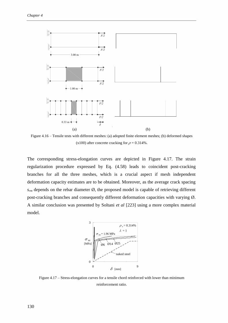
Chapter 4

130

(a) (b)

Figure 4.16 – Tensile tests with different meshes: (a) adopted finite element meshes; (b) deformed shapes

(x100) after concrete cracking for = 0.314%.

The corresponding stress-elongation curves are depicted in Figure 4.17. The strain

regularization procedure expressed by Eq. (4.58) leads to coincident post-cracking

branches for all the three meshes, which is a crucial aspect if mesh independent

deformation capacity estimates are to be obtained. Moreover, as the average crack spacing

srm depends on the rebar diameter Ø, the proposed model is capable of retrieving different

post-cracking branches and consequently different deformation capacities with varying Ø.

A similar conclusion was presented by Soltani et al [223] using a more complex material

model.

0

3

0 9 [mm]

xx

[MPa]

x = 0.314%

xu = 1.96 MPa

Ø6 Ø14 Ø25

naked steel

= 1

Figure 4.17 – Stress-elongation curves for a tensile chord reinforced with lower than minimum

reinforcement ratio.


131

If the reinforcement content is larger than the minimum, the strains in the post-cracking

stage no longer localize in one single finite element. A tensile test was again simulated

using the three meshes of Figure 4.16 (a), but this time using a reinforcement ratio of

= 1%. The tensile strength was randomly distributed along the mesh (with a mean value

of fct = 2.6MPa) in order to avoid simultaneous formation of cracks in all the finite

elements, thus reflecting the real crack pattern development more closely.

0

6

0 12 [mm]

xx

[MPa]

x = 1.0%

1 element mesh

naked steel

= 1

0

6

0 12 [mm]

xx

[MPa]

x = 1.0%

3 element mesh

naked steel

= 1

0

6

0 12 [mm]

xx

[MPa]

x = 1.0%

9 element mesh

naked steel

= 1

Figure 4.18 – Stress-elongation curves for a tensile chord reinforced with higher than minimum

reinforcement ratio.

The results of the simulations are presented in Figure 4.18. A brittle tensile concrete

behaviour was adopted in order to emphasize the effect of the reinforcement model. During

the crack formation stage, the curves differ amongst the three meshes. The saw-toothed

aspect of the stress-elongation curves is due to the sequential formation of cracks. The

number of teeth equals the number of finite elements in the mesh. As expected, in the

stabilized cracking stage all the three curves coincide. In this case, the rebar diameter

exerts no influence of the post-cracking curves.

Push off tests with passive confinement

In this numerical test, the combined behaviour of both the crack shear stress transfer and

reinforcement models is evaluated. A uniaxially reinforced quadrilateral element was

firstly pre-cracked in uniaxial tension and stretched until reaching xx = 0.371x10-3

. This

corresponds to the end of the first phase of loading, as indicated in Figure 4.19. In a second

phase, shear forces were applied. In this case, confinement is only exerted by the

reinforcement steel. Due to shear dilatancy, the reinforcement stresses increase with the

applied shear forces. The adopted material properties are the same as above, that

is cf =30MPa, fct = 2.6 MPa, fsy,x = fsy,y = 500MPa, fsu,x = fsu,y = 625MPa, su,x = su,y = 50‰

and Es = 200GPa.

Chapter 4

132

Figure 4.19 – Push-off tests with passive confinement (variable crack opening).

Several analyses were performed and the results are presented in Figure 4.20. The

influence of the rebar diameter, reinforcement content and crack spacing on the crack shear

behaviour is illustrated. In all the presented analyses, shear failure occurred after

reinforcement yielding.

0

10

0 0.006 xy

xy

[MPa]

x = 1.0%

= 1

Ø12 Ø25 Ø6

0

10

0 0.006 xy

xy

[MPa]

x = 0.5% = 1

Ø12

1%

2%

0

10

0 0.006 xy

xy

[MPa]

x = 1.0%

= 1

Ø12

= 0.5

0

0.006

0 0.006 xy

xx

Ø12

Ø25

Ø6

x = 1.0%

= 1

0

0.006

0 0.006 xy

xx

x = 0.5%

1%

2% = 1

Ø12

0

0.006

0 0.006 xy

xx

Ø12

x = 1.0%

= 0.5

= 1

Figure 4.20 – Push off tests with passive confinement: (a) effect of the rebar diameter; (b) effect of the

reinforcement content; (c) effect of the crack spacing.

Another test was additionally performed consisting in the application of reversed cyclic

shear loading in phase 2 with increasing cycling amplitude. The results are depicted in

Figure 4.21, where the numbers indicate the loading sequence. It can be seen that the

proposed formulation renders physically consistent results.


133

-6

0

6

-0.003 0 0.003 xy

xy

[MPa]

x = 1.0%

= 1

2

Ø25

1

3

4

5

6

-6

0

6

0 0.003 xx

xy

[MPa]

2

1

3

4

5

6

Figure 4.21 – Cyclic push off tests with passive confinement.

4.4 Extension to shell elements

The extension of the proposed algorithm from plane stress to shell elements substantially

enlarges the range of applicability of the proposed model to more general structural forms.

In the present formulation, the shell element is assumed as a series of juxtaposed layers

subjected to in-plane forces. This means that out-of-plane shear nonlinear effects are not

accounted for and only out-of-plane bending is considered besides the in-plane shear and

axial stresses. If out-of-plane shear is suspected to govern the behaviour, the Critical Shear

Crack Theory [81; 164; 166; 196] can be used together with the proposed models to

determine the shear resistance and corresponding deformation capacity, as outlined in the

report [82]. This theory can make use of the bending deformations for determining the

shear and punching strengths of slabs and beams. However, the analysis of out-of-plane

shear effects is out of scope of the present work.

Polak and Vecchio [188] undertaken a test program to investigate the behaviour of shell

elements subjected to biaxial bending and in-plane load conditions. The four test

specimens were panels 1524x1524x316 mm in dimension reinforced with two layers of

deformed bars in each of the two orthogonal directions. The specimens were subjected to

various combinations of biaxial bending and in-plane loads using the ―Shell-Element

Tester‖ at the University of Toronto. Details regarding the test parameters are given in

Table 4.1.

Specimen SM1 was loaded in pure uniaxial bending along the stronger reinforcement

direction. The loading of SM2 involved uniaxial bending coupled with in-plane tensile

forces in-line with the stronger reinforcement. Specimen SM3 was tested in pure biaxial

bending. Of particular interest are the results of test SM4 because of the skew direction of

Chapter 4

134

the reinforcement with respect to the applied bending and in-plane tensile forces.

Significant reorientation of the stress fields was reported when the weaker reinforcement

yielded.

Table 4.1 – Test parameters

Name cf Reinforcement

pattern

xc y

c

Loading pattern Loading

ratio [MPa] [%] [%]

SM1 47

1.25a

0.42b

-

SM2 62

1.25 a 0.42

b

M/P = 0.25 m

SM3 56

1.25 a 0.42

b

M1/M2 = 3.2

SM4 64

1.32 a 0.44

b

M/P = 0.25 m

a fsx = 425MPa, Øx = 19.5 mm

b fsy = 430MPa, Øy = 11.3 mm

c per layer

Since a uniform state of stress and strain was applied to the specimens, these were

modelled using one single finite element with four nodes. Five layers were used and the

Simpson integration rule is used along the layer thickness. Five integration points were

used in the inner layer while only three were used in the others. Predicted and observed

moment-curvature responses are compared in Figure 4.22. Good correlation is observed,

thus providing further validation to the proposed model. In the tensioned layers of

specimen SM4 two orthogonal cracks developed and shear stresses were induced due to

the skew direction of the reinforcement. In this case, stiffness degradation is more gradual.

Even in this demanding situation the proposed algorithm revealed good convergence

characteristics.


135

0

500

0 0.04

Mom

ent

[kN

.m/m

]

Curvature (rad/m)

F-CMM

Exp.

SM1

, = 1

, = 1

, = 0

, = 0

x,0 = - 2.07 MPa

0

500

0 0.04

Mom

ent

[kN

.m/m

]

Curvature (rad/m)

F-CMM

Exp.

SM2

0

500

0 0.04

Mom

ent

[kN

.m/m

]

Curvature (rad/m)

F-CMM

Exp.

SM3

x- direction

y- direction

0

500

0 0.06

Mom

ent

[kN

.m/m

]

Curvature (rad/m)

F-CMM

Exp.

SM4

Figure 4.22 – Moment vs. curvature relationships for the panels of the SM series


The basic concepts behind the computational models for nonlinear analysis of structural

concrete elements were presented and a total strain constitutive model for accommodating

the RC cracked membrane element constitutive laws devised in Chapter 3 was developed.

The implemented algorithm was described in detail and some simple validation examples

were presented to illustrate the model response. The implementation was extended to shell

elements and good agreement was obtained when comparing the calculated results with

experimental data collected on RC shell elements subjected to bending and membrane

loads. Good convergence characteristics were exhibited in the analysed examples. The

validation of the proposed model at the structural level is presented in the following

chapter.

137

5 Analysis of shear critical elements

5.1 General

Following the previously performed validation at element level, which included the

extensive set of RC panels analysed in Chapter 3, in this chapter the validation at the

structural level of the proposed constitutive model is presented. This validation is made

using a set of experimental tests on large scale structural elements, which were criteriously

selected to provide a stringent test to the capabilities of the model. In general, the

validation presented here was targeted at evaluating the accuracy of the model in the: (1)

calculation of shear failure loads and corresponding failure mechanisms; (2) determination

of the load-deformation curves and of the deformation capacity of large scale beams; (3)

simulation of the observed cracking patterns and calculation of the corresponding crack

widths. Each of the selected test series represents a specific feature of the structural

behaviour that should be properly modelled in order to allow improved structural analyses

of existing concrete bridges. Where appropriate, comparisons with codes of practice are

presented for reference.

All the required concrete related parameters are calculated automatically from cf according

to what has been exposed previously. Therefore, cf is the only concrete related parameter

that needs to be specified. The only remark goes to the parameter fc0. In Chapter 3, fc0 was

taken equal to 20MPa. However, in the following examples better estimates of the

effective concrete compressive strength fc,ef were obtained with fc0 = 30MPa. This fact can

be attributed to some degree of out of plane confinement that is present in the critical

regions of the webs, thereby delaying the splitting failure mode.

The structural elements were modelled with 8 node plain stress finite elements using the

default 2x2 Gaussian integration rule. The reinforcement contribution is directly taken into

account in the constitutive laws. Therefore, there is no need for using dedicated finite

elements for modelling the reinforcements. However, embedded truss elements are

required for modelling the post-tensioning cables or prestressing strands, for which the

available elements in the DIANA element library are used.

Chapter 5

138

5.2 Shear in continuity regions

5.2.1 Description and objectives

The goal of the VN test series presented in this section was to investigate the behaviour of

webs of structural concrete girders with no plastic deformation in the chords, having low

shear reinforcement ratios (w=0.335%) and correspondingly flat inclinations of the

concrete compressive struts at failure. The state of stress is similar to that observed outside

the support regions of a continuous girder (Figure 5.1). These specimens can be assumed to

reproduce the behaviour of typical continuity, or B-, regions. For that purpose a dedicated

testing facility was developed by Kaufmann and Marti at ETH Zürich, allowing the

investigation of elements of beams rather than entire girders. For further details refer to test

report [119].

Figure 5.1 – Internal forces in the beams of the VN series.

The VN series is constituted by four identical 5.84m long and 0.78m high I-shaped beam

segments. These were monotonically loaded in shear until failure with zero moment at

midspan, as shown in Figure 5.1. The longitudinal reinforcement was designed to remain

elastic during the test. The specimens VN1 and VN3 were pre-cracked in tension before

the application of the shear forces and are not analysed here. The specimen VN4 differs

from VN2 because it was subjected to a constant compressive axial force of N = 1 MN

(which is equivalent to an initial uniform compressive stress of 3.2MPa). The geometry

and reinforcement content of the beams are presented in Figure 5.2 together with the

adopted finite element mesh. The shaded elements in Figure 5.2 (c) were included to

reproduce the real external force eccentricities with respect to the beam. The material

Analysis of shear critical elements

139

properties are given in Table 5.1. The zones corresponding to different material properties

are identified in Figure 5.2 (c).

(a)

(b) (c)

Figure 5.2 – VN series: (a) Geometry; (b) Reinforcement content; (c) Finite element mesh. The black dots

indicate the nodes whose displacements were used for calculating the average web deformations.

Table 5.1 – Material properties of the beams VN2 and VN4

Zone t

[m]

f ’c

[MPa]

x [%]

Øx

[mm]

fsy,x

[MPa]

fsu,x

[MPa]

su,x

[‰]

y [%]

Øy [mm]

fsy,y

[MPa]

fsu,y

[MPa]

su,y

[‰]

F1 0.80

52.6

(VN2)

61.9

(VN4)

1 8.849 26 539 644 118 0.126 8 510 604 53

W1 0.15 0.5 0.558 8 510 604 53 0.335 8 510 604 53

W2 0.258 0.5 0.682 8 510 604 53 0.628 8 510 604 53

W3 0.475 0.5 0.370 8 510 604 53 0.352 8 510 604 53

W4 0.692 0.5 0.254 8 510 604 53 0.242 8 510 604 53

Due to the small amount of stirrups, large web crack spacings could be expected if these

were only governed by the web reinforcement content. In the webs, the crack spacing is

often governed not only by the web reinforcement but also by the crack spacing in the

tension chord. Therefore, in the analyses presented in this chapter different values were

adopted for the parameter in the flanges and in the webs. Unless otherwise stated, the

maximum crack spacing ( = 1) was considered in the flanges and the minimum crack

spacing ( = 0.5) was adopted in the webs. Although some fine tuning could be performed,

Chapter 5

140

reasonable estimates of the crack spacing and crack widths were generally obtained. In the

case of beamVN4, the axial force was applied in the first loading step. Afterwards the

shear force F was incremented until failure, see Figure 5.2 (c).

5.2.2 Results

5.2.2.1 Failure loads and failure mechanims

Collapse was governed by failure of the web in the central portion of the girders in all the

tests. In girder VN2, collapse was triggered by stirrup rupture with some spalling of the

web concrete cover. Specimen VN4 exhibited a web crushing failure. These failure modes

were accurately predicted by the F-CMM. The R-CMM predicts web crushing failures for

both VN2 and VN4. The failure loads and failure modes are summarized in Table 5.2. It

can be seen that the limitation on the inclination of the web struts governs the ultimate

loads predicted by the EC2 [46] variable angle truss model. The F-CMM provides the best

estimates of the failure loads.

Table 5.2 – Comparison between experimental and calculated failure loads and failure modes

Experimental F-CMM R-CMM EC2

N

[kN]

Vu

[kN]

Mode (1)

Vu

[kN]

Mode (1)

Rat. (2)

Vu

[kN]

Mode (1)

Rat. (2)

Vu

[kN]

Mode (3)

Rat. (2)

VN2 0 548 SF 537 SF 1.02 565 WC 0.97 404 S 1.36

VN4 1000 564 WC 566 WC 1.00 604 WC 0.93 404 S 1.40

(1)Failure mode: SF – Stirrup failure; WC – web crushing failure; WS – web sliding failure

(2)Failure load ratio: Vu,exp / Vu,calculated

(3)Failure mode according to the EC2 variable angle truss model: S – failure governed by the stirrups (in this

case, the limitation on the inclination of the struts to cot = 2.5 governs); C – failure governed by crushing

of the web.

In the case of cracked concrete, the state variable Emax = -t / 0,ef is an indicator of whether

concrete crushing has or not occurred. If Emax >1 the post-peak branch of the stress strain

curve has been achieved. In this stage of the curve, signs of concrete cover spalling or

concrete delamination are to be expected in real specimens. The contour levels with the

values of Emax at failure are presented in Figure 5.3. It can be seen that the F-CMM predicts

only minor signs of web cover spalling near the flanges for beam VN2. Similarly to the test,

collapse was triggered by rupture of the vertical reinforcement. This can be confirmed in

Figure 5.4, where the contour levels with the vertical reinforcement stresses at the cracks

are presented. The red colour corresponds to regions where the tensile strength of the


141

stirrups (fsu = 604 MPa) was exceeded. In the case of the R-CMM, the stresses in the

vertical reinforcement are well below this value.

(a) VN2

(b) VN4

Figure 5.3 – Deformed shape (x10) with the Emax contour levels at failure.

Figure 5.4 – Beam VN2: deformed shape (x10) at peak load with the contour levels representing stirrup

stresses at the cracks (in Pa).

5.2.2.2 Force-deformation curves

In Figure 5.5 the calculated and the measured average deformations in a 1.60m (from

x = -0.80 m to x = +0.80m) long web segment at the centre of the beams are compared. In

the test, the average deformations where obtained from the relative displacements between

targets positioned in the webs or in the flanges of the beams, which explains the two curves

for the experimental results presented in each plot. The values corresponding to the

numerical results were determined from the displacements of the nodes indicated in Figure

Chapter 5

142

5.2. Parameter y is the average vertical strain within the measuring domain, 2 is the

average principal compressive strain and e is the angle of the principal average

compressive strain with the beam longitudinal axis. The agreement between the calculated

and the measured force-deformation curves is good, especially for the F-CMM. The R-

CMM tends to overestimate the stiffness after stirrup yielding. In the case of beam VN2,

stirrup failure is predicted by the F-CMM, but for an average vertical strain that is smaller

than that observed in the test. This can be attributed to the fact that the model cannot

reproduce bond slip occurring across several cracks. A close inspection to the picture of

beam VN2 at failure presented in Figure 5.6 (a) reveals that stirrup debonding is likely to

have occurred in the test. Therefore, conservative estimates of the stirrups deformation

capacity are to be expected in similar cases. The angle e is accurately predicted, which is

an indication that both the crack kinematics and inclination of the struts are well

reproduced. At failure, e values down to 15º were obtained.

0

700

0 30 y (x10

3)

F [

kN

]

Exp.

Exp.

F-CMM

R-CMM

LS1

LS2

LS3LS4 LS5

Peak load

VN2

0

700

-3 0 2 (x10

3)

F [

kN

] Exp.

F-CMM

R-CMM

Exp.

VN2

0

700

-45 0 e (x10

3)

F [

kN

] Exp.

F-CMM

R-CMM

Exp.

VN2

0

700

0 30 y (x10

3)

F [

kN

]

Exp.

Exp.

F-CMM

R-CMM

Peak load

LS1

LS2

LS3LS4

LS5

VN4

0

700

-3 0 2 (x10

3)

F [

kN

] Exp.

F-CMM

R-CMM

Exp.

VN4

0

700

-45 0 e (º)

F [

kN

] Exp.

F-CMM

R-CMM

Exp.

VN4

Figure 5.5 – Force vs. average deformation related parameters. Manual measurements were made at the

load steps LSi.

5.2.2.3 Cracking patterns

The experimental and calculated cracking patterns at failure are presented in Figure 5.6 and

Figure 5.7. The calculated cracking patterns are represented by lines with the direction of

the crack. Its thickness is proportional to the crack opening using a three level scale.


143

(a) Experiment [119]

(b) F-CMM

(c) R-CMM

Figure 5.6 – Beam VN2: cracking patterns at failure.


(b) F-CMM

(c) R-CMM

Figure 5.7 – Beam VN4: cracking patterns at failure.

The crack angles and the crack widths are presented in Figure 5.8. The load steps LSi are

identified in Figure 5.5. The crack angles are better predicted by the F-CMM. By allowing

continuous crack rotation, the crack angles calculated with the R-CMM tend to deviate

from the measured ones as loading progresses. The crack width predictions in the webs are

reasonably fitted to the measurements, although some underestimation of the maximum

crack width is observed in the first load stages. However, in these stages the cracking

pattern is not yet stabilized and increased scatter must be expected.

Chapter 5

144

0

45

-2 0 2

x [m]

Cra

ck a

ng

le (

deg

)

F-CMM R-CMM (LS1)

R-CMM (LS3) R-CMM (LS4)

Exp.

0

45

-2 0 2

x (m)

Cra

ck a

ng

le (

deg

)

F-CMM R-CMM (LS2) R-CMM (LS5)

Exp.

0

2.5

-2 0 2

x (m)

wr (m

m)

F-CMM

R-CMM

LS 4 Exp.

0

2.5

-2 0 2

x (m)

wr (m

m)

F-CMM

R-CMM

LS 5 Exp.

0

1.6

-2 0 2

x (m)

wr (m

m)

F-CMMR-CMMExp.

LS 3

0

1.6

-2 0 2

x (m)

wr (m

m)

F-CMMR-CMM

LS 4

Exp.

0

0.8

-2 0 2

x (m)

wr (m

m)

F-CMMR-CMMExp.

LS 2

0

0.8

-2 0 2

x (m)

wr (m

m)

F-CMMR-CMM

LS 3

Exp.

0

0.5

-2 0 2

x (m)

wr (m

m)

F-CMMR-CMMExp.

LS 1

0

0.5

-2 0 2

x (m)

wr (m

m)

F-CMMR-CMM

LS 2

Exp.

(a) VN2 (b) VN4

Figure 5.8 – Crack angles and crack widths compared to experimental evidence: (a) VN2; (b) VN4.


145

5.3 Shear in discontinuity regions with plastic reinforcement

strains


The four beams of the series MVN have the same geometry and the same shear

reinforcement content as the ones from the series VN. However, in contrast to series VN,

an additional vertical jack was installed at midspan. The loading procedure simulated the

behaviour of an (inverted) intermediate support of a continuous girder, see Figure 5.9. In

this case, bending moments may have a significant influence on the behaviour of the girder

and usually chords are plastically deformed. Note that this bending-shear interaction is not

directly taken into account in the lower bound limit analysis methods specified in codes of

practice. Contrary to the series VN, in these specimens failure is expected to occur in a

typical discontinuity, or D-, region.

Figure 5.9 – Internal forces in the beams of the MVN series.

In the first phase of the test, horizontal forces were controlled such that moments at the

element ends were null. In the second phase, after reaching the yield moment at midspan,

rotations at the element ends were prevented. This second phase of the test simulated a

redistribution of moments from the support region (midspan) to the span (element ends) of

a continuous girder. The forces applied at the element ends were controlled so that normal

forces remained constant throughout the test and shear forces on either side of the

concentrated load were of equal magnitude.

All the girders contained the same amount of web reinforcement: w=0.335%, equal to the

one adopted in the series VN. Regarding the longitudinal reinforcement, specimens MVN1

Chapter 5

146

to 3 were designed to reach the yield moment at midspan under the same net web shear (i.e.

total shear minus the contribution of the inclined post-tensioning cable as shown below).

MVN4 was designed not to yield at midspan during the entire test. Specimens MVN2 and

MVN4 were subjected to axial compression of 1.30 MN before being loaded in shear and

the axial force was held constant during the test. Specimens MVN3 and MVN4 were post-

tensioned with a bonded VSL 6-7 cable (Pu = 1.85 MN) with an initial target force of

1.30 MN. Therefore, the initial horizontal compressive stresses in the beams were null for

MVN1, 4.2MPa for MVN2 and MVN3, and 8.4MPa for MVN4. The cable layout and the

reinforcement content of the beams are presented in Figure 5.10.

(a) Cable layout (MVN3 and MVN4)

(b) MVN1 (c) MVN2

(d) MVN3 (e) MVN4

Figure 5.10 – MVN series: (a) Cable layout of beams MVN3 and MVN4; (b) reinforcement content.


147

(a) Phase 1

(b) Phase 2

Figure 5.11 – MVN series: finite element mesh. The black dots indicate the nodes whose displacements

were used for calculating the average web deformations.

Table 5.3 – Material properties of the beams MVN1 to MVN4

Zone t

[m]

f ’c

[MPa]

x [%]

Øx(2)

[mm]

fsy,x(2)

[MPa]

fsu,x(2)

[MPa]

su,x(2)

[‰]

y [%]

Øy [mm]

fsy,y

[MPa]

fsu,y

[MPa]

su,y

[‰]

MVN1

F1

0.80 62.8 1

2.356 16 524 652 128 0.126

8 461 580 87 F2 3.142 16 528 660 127 0.378

F3 1.571 16 524 653 130 0.126

MVN2

F1

0.8 58.8 1

1.309 16 518 642 128 0.126

8 461 580 87 F2 2.094 16 526 656 127 0.378

F3 1.571 16 524 653 130 0.126

MVN3

F1

0.8 62.2 1

0.785 10 508 625 131 0.126

8 461 580 87 F2 2.094 16 526 656 127 0.378

F3 1.571 16 524 653 130 0.126

MVN4

F1

0.8 64.3 1

2.356 16 524 652 128 0.126

8 461 580 87 F2 1.571 16 524 653 130 0.378

F3 1.571 16 524 653 130 0.126

MVN1 to MVN4

W1 0.15

(1)

0.5 0.558

8 461 580 87

0.335

8 461 580 87

W2 0.258 0.5 0.682 0.628

W3 0.475 0.5 0.370 0.352

W4 0.692 0.5 0.254 0.242

(1) For each beam, the uniaxial cylinder strength of the web concrete is the same adopted for the flanges.

(2) In the case of rebars with different diameters and steel properties, a weighted average value was adopted.

The adopted finite element mesh is depicted in Figure 5.11. The compatibility of the

vertical displacements between the loading platen and the upper flange elements was

enforced while the corresponding relative horizontal displacements were allowed. The

Chapter 5

148

prestressing tendon was modelled using embedded reinforcement elements [256]. A

bilinear stress-strain law was adopted with fpy = 1713 MPa, fpu = 1866 MPa, pu = 60‰ and

Ep = 190 GPa. The adopted material properties are presented in Table 5.3. The zones

corresponding to distinct reinforcement contents and element thicknesses are identified in

Figure 5.11. In the first step the self-weight, the axial force and the post-tensioning force

were applied. Only after the force F was incrementally increased. When the bottom

longitudinal reinforcement started yielding, the boundary conditions were modified

according to Figure 5.11 for the second phase of the test.

5.3.2 Results

5.3.2.1 Failure loads and failure mechanisms

The failure loads and the failure modes are summarized in Table 5.4. The calculated

ultimate loads are in good agreement with the observed ones. The effect of the applied

normal and prestressing forces significantly influenced the failure mode and failure loads

experienced by the tested specimens. The limitation on the inclination of the web struts

governs the ultimate loads predicted by the EC2 [46] variable angle truss model. Three

different failure modes were observed in the tests. The contour levels of the state variable

Emax at peak load are presented in Figure 5.12 for the MVN1 and MVN4 specimens.



N

[kN]

P0

[kN]

Fu

[kN]

Mode (1)

Fu

[kN]

Mode (1)

Rat.

(2)

Fu

[kN]

Mode (1)

Rat.

(2)

Fu

[kN]

Mode (3)

Rat.

(2)

MVN1 0 0 1063 SF 1040 SF 1.02 1157 WC 0.92 730 S 1.46

MVN2 1300 0 1208 WS 1206 WS/WC 1.00 1202 WC 1.00 730 S 1.65

MVN3 0 1300 1760 WS 1627 WC 1.08 1594 WC 1.10 1020 S 1.73

MVN4 1300 1250 1950 WC 1787 WC 1.09 1731 WC 1.13 1020 S 1.91

(1)Failure mode: SF – Stirrup failure; WC – web crushing failure; WS – web sliding failure.

(2)Failure load ratio: Fu,exp / Fu,calculated.

(3)Failure mode according to the EC2 variable angle truss model: S – failure governed by the stirrups (in this

case, the limitation on the inclination of the struts to cot = 2.5 governs); C – failure governed by crushing

of the web.

The collapse of beam MVN1 was initiated by the rupture of a stirrup after some spalling of

the web concrete cover. Once again, this failure mode was accurately predicted by the

F-CMM, while the R-CMM predicted a web crushing failure.


149

The specimens MVN2 and MVN3 failed in a similar manner: half of the girder shifted

over the remaining part of the element along an inclined failure surface made up of

existing web shear cracks, with crushing of concrete in the flange. Spalling of the concrete

cover in the web was observed, notably in specimen MVN3, which indicates crushing of

the concrete in the web. This failure mode is here classified as a web sliding failure. By

definition, this failure mode cannot be reproduced by the R-CMM and this model predicts

web crushing failures for both specimens. As it was shown in the previous chapter, the

F-CMM can reproduce such type of failure in RC panels. However, the web compressive

stresses are rather high and crushing ends up to govern the computed failure mode.

Nonetheless, in the case of MVN2 collapse occurred after concrete crushing in the top

flange, near the loading platen. This can be confirmed by the incremental deformed shape

in the post peak branch of the load-deformation curves, see Figure 5.13, which is an

indication of the occurrence of a sliding shear failure. Although the localization of the

crack shear strains nt along an inclined band can be seen in Figure 5.13, this localization is

not sharp enough to properly reproduce the sliding movement along the failure crack.

(a) MVN1

(b) MVN4

Figure 5.12 – Deformed shape (x10) after peak load with the contour levels of the state variable Emax.

Figure 5.13 – Failure mode of beam MVN2 as calculated with the F-CMM: incremental deformed shape

(x1000) after the peak load with the contour levels of the crack shear strains nt.

The specimen MVN4 exhibited a web crushing failure. Failure was more ductile and the

web concrete crushed progressively on both sides of the girder. This failure mode was

correctly predicted by both the F-CMM and R-CMM. However, in both numerical analyses

strain localization is observed in the web near the upper flange, see Figure 5.12 (b). This

localization of the compressive strains is much more pronounced than the observed in the

Chapter 5

150

experiment, where the crushing failure progressed in several regions of the web. This is an

intrinsic limitation of the adopted kinematic description of the displacement field based on

the weak-discontinuities concept.


The calculated and measured average deformations are compared in Figure 5.14. Defor-

mations were averaged over two symmetrically located and 0.80 m long web segments

(from x = ±1.20 m to x = ±2.00 m). The numerical results were calculated from the relative

displacements of the nodes indicated in Figure 5.11.

0

2000

0 20 y (x10

3)

F [

kN

]

Exp.

Exp.

F-CMM

R-CMM

Peak load

MVN1

0

2000

-3 0 2 (x10

3)

F [

kN

] Exp.

F-CMM

R-CMM

Exp.

MVN1

0

2000

0 45 e (x10

3)

F [

kN

] Exp.

F-CMM

R-CMM

Exp.

MVN1

0

2000

0 20 y (x10

3)

F [

kN

]

Exp.

Exp.

F-CMM

R-CMM

Peak load

MVN2

0

2000

-3 0 2 (x10

3)

F [

kN

] Exp.

F-CMM

R-CMM

Exp.

MVN2

0

2000

0 45 e (x10

3)

F [

kN

] Exp.

F-CMM

R-CMM

Exp.

MVN2

0

2000

0 20 y (x10

3)

F [

kN

]

Exp.

Exp.

F-CMM

R-CMM

Peak load

MVN3

0

2000

-3 0 2 (x10

3)

F [

kN

] Exp.

F-CMM

R-CMM

Exp.

MVN3

0

2000

0 45 e (x10

3)

F [

kN

] Exp.

F-CMM

R-CMM

Exp.

MVN3

0

2000

0 20 y (x10

3)

F [

kN

] Exp.

Exp.

F-CMM

R-CMM

MVN4

Peak load

0

2000

-3 0 2 (x10

3)

F [

kN

] Exp.

F-CMM

R-CMM

Exp.

MVN4

0

2000

0 45 e (º)

F [

kN

] Exp.

F-CMM

R-CMM

Exp.

MVN4

Figure 5.14 – Force vs. average deformation related parameters.


151

In general, the agreement between the measurements and the calculations is good. It must

be remarked that these are average web strains which are directly related with the shear

behaviour. Usually, a good fit between numerical and experimental results is easier to

obtain if flexure related parameters (midspan displacements, for instance) are compared.

The exception lies in the fit between the predicted and measured average vertical strains y

for specimen MVN1, which is rather poor. An overly stiff F-y curve is computed with the

F-CMM. This might be due to the fact that, in the test, the shear cracks in the vicinity of

the vertical jack propagate through previously formed vertical flexural cracks. As

discussed previously, this cannot be modelled by the F-CMM because only orthogonal

cracks are allowed. In the other three tests this phenomenon was not observed and the

agreement is significantly better. Still regarding specimen MVN1, the overestimation of

the stiffness of the F-y curve exhibited by the R-CMM is somewhat more difficult to

explain. A similar behaviour was observed in the analysis of the panel PP1 (see Chapter 3)

and of the beams VN2 and VN4. Although not so evident as in this case, it was then

noticed that the R-CMM over-predicted both the stiffness and the ultimate shear stress of

elements exhibiting significant crack shear slip in the experimental tests.

The analysis of the curves in Figure 5.14 also shows that the principal compressive strains

are systematically overestimated with R-CMM. This is more noticeable in the cases where

less crack shear slip is expected due to the external axial forces. In these cases, the use of a

softened peak uniaxial strain in the cracked concrete stress-strain relationship could

improve the results. However, this would worsen the performance in the other cases, since

in the rotating crack model the crack shear slip is not independently modelled.


The experimental and calculated cracking patterns at failure are presented in Figure 5.15 to

Figure 5.18. In general, the calculated crack patterns provide a good picture of the real

ones. The shear failure plane of specimens MVN2 and MVN3 is not clearly evidenced in

the numerical simulations due to the fact that crushing of the web concrete governed the

computed failure mode, as described above.

The crack angles are compared in Figure 5.19. The F-CMM provides good estimates of the

crack inclination and the effect of normal stresses is well reproduced. Similarly to what has

been observed in the VN series, the crack angles predicted by the R-CMM tend to deviate

from the measured ones as the loading progresses.

Chapter 5

152


(b) F-CMM

(c) R-CMM

Figure 5.15 – Beam MVN1: cracking patterns at failure.


(b) F-CMM

(c) R-CMM



(b) F-CMM

(c) R-CMM



153


(b) F-CMM

(c) R-CMM


0

90

-2 0 2

x [m]

Cra

ck a

ng

le (

deg

)

F-CMM

R-CMM (LS1)

R-CMM (LS2)

Exp.

MVN1

0

90

-2 0 2

x [m]

Cra

ck a

ng

le (

deg

)

F-CMM

R-CMM (LS1)

R-CMM (LS2)

R-CMM (LS3)

Exp.

MVN2

0

90

-2 0 2

x [m]

Cra

ck a

ng

le (

deg

) F-CMM

R-CMM (LS1)

R-CMM (LS2)

R-CMM (LS3)

Exp.

MVN3

0

90

-2 0 2

x [m]

Cra

ck a

ng

le (

deg

)

F-CMM

R-CMM (LS1)

R-CMM (LS2)

R-CMM (LS3)Exp.

MVN4

Figure 5.19 – Web crack angles for specimens MVN1 to MVN4.

5.3.2.4 Shear force carried by the various elements of the girders

It is interesting to evaluate the contribution of each element of the girder – web, flanges,

and prestressing tendons – for the shear load carrying capacity. The numerical analyses

allow performing such investigation. The results obtained with the F-CMM are plotted in

Figure 5.20. The important role of the upper flange can be noted in the beams of the MVN

series in the regions closer to mid-span, while in the beam VN4 this contribution is not so

significant, as should be expected in a continuity region.

Chapter 5

154

0

1

-0.5 0x / L

Vi / V

Series2

Series1

Vweb

Vupper flange

Vlower flange

0

1

0 0.5x / L

Vi / V

Series2

Series3

Series1

Vweb

Vupper flange

Vlower flange

Vprestress

0

1

-0.5 0 0.5

x / L

Vi / V Vweb

Vupper flange

Vlower flange

Figure 5.20 – Shear forces carried by the various elements of the girders.


155

5.4 High strength concrete girders critical in shear


This testing program was performed for the NCHRP at the University of Illinois under the

supervision of Hawkins and Kuchma [94]. The study aimed at extending the applicability

of the shear provisions of the AASHTO LFRD Bridge Design Specifications [1] to

reinforced and prestressed concrete structures with concrete strengths above 70 MPa. A

total of twenty experiments on ten 1.85 m deep and 15.85 m long bulb-tee girders were

performed. The girders were simply supported with a span of 15.24 m and were subjected

to a uniformly distributed load over the central 13.41 m of their length. A 0.25 m deep slab

was cast over each girder. The overall geometry of the tested girders is presented in Figure

5.21.

(a)

(b) (c)

(d) (e)

Figure 5.21 – Geometry of the tested girders: (a) Elevation; (b) Cross-section; (c) Cross-section as

modelled; (d) West half of beam G1 with draped strands; (e) Finite element mesh.

Chapter 5

156

Each half of each girder (designated as East and West) was designed to be different so as

to obtain two test results from each girder. This was accomplished by reconstructing and

strengthening the half of the girder that failed first and then reloading the girder until the

other half failed. Here, only the girders G1, G2 and G5 are analysed. These girders have

vertical web reinforcement ratios in the failure zone of w = 0.56, 0.94 and 0.18%,

respectively. In girders G1 and G2, six prestressing strands were draped in the West end,

thus increasing the shear strength due to the vertical component of the prestressing force.

In girder G5, the difference between the East and West ends was the adoption of welded

wire reinforcement in the East end, while maintaining the diameters and the spacing

between the rebars.

(a)

(b)

Figure 5.22 – Cross-section: (a) Reinforcement content in the critical region; (b) Location of prestressing

strands.


157

The reinforcement arrangement within the cross-section and the location of the

prestressing strands are presented in Figure 5.22. The spacing between the strands layers

equals 50.8 mm. The measured effective initial prestress, p0, and the corresponding

transfer lengths, lt, of the prestressing force are also indicated in the figure. In all the

analyses, the initial prestress was assumed to vary linearly from zero up to p0 along the

transfer length. A bilinear stress-strain law was adopted for the prestressing steel with

fpy = 1675 MPa, fpu = 1860 MPa, pu = 50‰ and Ep = 195 GPa. The remaining material

properties are indicated in Table 5.5. It is remarked that reasonable estimates of the web

crack spacing for G5 were only obtained with = 0.3. The length of the web regions with

different amounts of stirrups is indicated in Table 5.6.

Table 5.5 – Material properties of the analysed beams belonging to the G series

Zone t

[m]

f ’c

[MPa] x [%]

Øx

[mm]

fsy,x

[MPa]

fsu,x

[MPa]

su,x(1)

[‰]

y [%]

Øy [mm]

fsy,y

[MPa]

fsu,y

[MPa]

su,y(1)

[‰]

G1E and G1W

F1 1.067 31.0 1 1.040 19 547 820 150 0.0 - - - -

W1

0.152 83.4 0.5 0.166 9.5 527 775 150

0.555

12.7 483 752 150 W2 0.278

W3

W4 5.160 15.9 547 820 150

G2E and G2W

F1 1.067 59.3 1 1.040 19 547 820 150 0.0 - - - -

W1

0.152 86.8 0.5 0.166 9.5 527 775 150

0.939 15.9 547 820 150

W2 0.608

W3 0.303 12.7 483 752 150

W4 5.160 15.9 547 820 150

G5E

F1 1.067 42.0 1 1.040 19 547 820 150 0.0 - - - -

W1

0.152 122.7 0.3 0.166 9.5(2)

637 732 100 0.183 9.5

(2) 637 732 100 W2

W3

W4 5.160 15.9 547 820 150

G5W

F1 1.067 42.0 1 1.040 19 547 820 150 0.0 - - - -

W1

0.152 122.7 0.3 0.166 9.5 527 775 150 0.183 9.5 527 775 150 W2

W3

W4 5.160 15.9 547 820 150

(1) Not indicated in the test report. Typical value for steel currently used in the US was adopted;

(2) Welded wire reinforcement.

Chapter 5

158

Table 5.6 – Length of the web regions with different amounts of stirrups

Girder

Length [m]

W1 W2 W3

G1 3.658 3.963 -

G2 3.658 2.438 1.524

G5 7.620 - -

The analyses were divided in two phases. In the first phase, only the finite elements

corresponding to the beam were activated. In this stage, the self weight and the pre-

stressing forces were applied matching the effective prestress and the transfer lengths lt

indicated in Figure 5.22 (b). In the second phase, the finite elements corresponding to the

slab were activated and the vertical load was incremented until failure.

5.4.2 Results


Collapse occurred in a similar manner for specimens G1E, G1W, G2E and G2W.

Concrete crushing occurred in the web immediately above the bottom bulb. This failure

mode was accurately predicted both by the F-CMM and the R-CMM. Representative

pictures of this failure mode are depicted in Figure 5.23 (a) and (b). The corresponding

contour levels with the state variable Emax in the post-peak stage are presented in Figure

5.23 (c). Although a band of crushed finite elements can be seen, concrete crushing started

immediately above the support and then progressed until the formation of the band

depicted in Figure 5.23 (c). This failure mode is largely influenced by support dimensions

and reinforcement detailing in the end region of the beams.

(a) (b) (c)

Figure 5.23 – Typical web crushing failure observed in the girders G1E,G1W, G2E and G2W: (a) East half

of girder G2 at failure [95]; (b) Detail of the end region [95]; (c) F-CMM analysis of the half girder G2E -

deformed shape (x10) with the Emax contour levels in the post-peak stage.


159

In the case of specimens G5E and G5W, a wide open shear crack dominated the behaviour.

In the East half, which was reinforced with welded wire mesh, a diagonal tension failure

occurred due to stirrup rupture, as depicted in Figure 5.24 (a). Both the F-CMM and the R-

CMM correctly predicted this failure mode, as can be observed from the contour levels

with the calculated stirrup stresses at the cracks presented in Figure 5.24 (b). The red

colour corresponds to regions where the tensile strength of the stirrups (fsu = 732 MPa) was

exceeded. The West half collapsed with local web concrete crushing above the support and

with significant sliding along the dominant web shear crack.

(a) (b)

Figure 5.24 – Diagonal tension failure of girder G5E: (a) East half of girder G5 at failure [95]; (b) F-CMM

analysis - deformed shape (x10) with the vertical reinforcement stress contour levels at peak load (values in

Pa and between fsy and fsu).

The failure loads and failure modes are summarized in Table 5.7. The F-CMM supplies

once again the best predictions of the failure loads. The failure load of the specimen G5E is

underpredicted with both models. However, it must be remarked that no information

regarding the ultimate tensile strain of the reinforcement was given in the test report and

that the failure mode is sensitive to this parameter. Although exhibiting good agreement

with the failure loads of girders G1 and G2, the precision of the Eurocode 2 [46] variable

angle truss model decays significantly when very low shear reinforcement ratios are used.

Nonetheless, the use of sectional models in this case is debatable as failure was governed

by local conditions at the ends of the specimens.

Chapter 5

160



qu

[kN/m] Mode

(1) qu [kN/m]

Mode(1)

Rat.(2)

qu

[kN/m] Mode

(1) Rat.

(2)

qu [kN/m]

Mode(3)

Rat.(2)

G1E 380 WC 371 WC 1.02 333 WC 1.14 371 S 1.02

G1W 439 WC 423 WC 1.04 374 WC 1.17 414 S 1.06

G2E 493 WC 489 WC 1.01 461 WC 1.07 515 B 0.96

G2W 565 WC 515 WC 1.10 468 WC 1.21 515 B 1.10

G5E 346 SF 300 SF 1.15 282 SF/WC 1.23 185 S 1.87

G5W 291 WC/WS 291 WC/WS 1.00 279 WC 1.04 153 S 1.90

(1) Failure mode: SF – Stirrup failure; WC – web crushing failure; WS – web sliding failure;

(2) Failure load

ratio: Fu,exp / Fu,calculated; (3)

Failure mode according to the EC2 variable angle truss model: S – failure governed

by the stirrups; C –failure governed by crushing of the web; B – bending failure.


The force vs. midspan displacement curves for all the analysed beams are depicted in

Figure 5.25 and in general good agreement can be found between the calculated and the

measured curves.

0

600

0 150 1/2 [mm]

q [

kN

/m]

Exp.

F-CMM

R-CMM

LS1

LS2

LS3

LS4

LS5

Peak loadG1E

0

600

0 150 1/2 [mm]

q [

kN

/m]

Exp.

F-CMM

R-CMM

LS1

LS2

LS3

LS4

LS5

Peak loadG2E

0

600

0 150 1/2 [mm]

q [

kN

/m]

Exp.

F-CMM

R-CMM

LS1

LS2

LS3

LS4

LS5

Peak loadG5E

0

600

0 150 1/2 [mm]

q [

kN

/m]

Exp.

F-CMM

R-CMM

LS1

LS2

LS3

LS4

LS5

Peak loadG1W

0

600

0 150 1/2 [mm]

q [

kN

/m]

Exp.

F-CMM

R-CMM

LS1

LS2

LS3

LS4

LS5

Peak loadG2W

0

600

0 150 1/2 [mm]

q [

kN

/m]

Exp.

F-CMM

R-CMM

LS1

LS2

LS3

LS4

LS5

Peak loadG5W

Figure 5.25 – Distributed force vs. midspan displacement.

It can be shown that - with the adopted value for the yielding stress of the prestressing steel

- the yielding moment at midspan is reached when q = 432, 515 and 340 kN/m for beams

G1, G2 and G5, respectively. In the G2W experiment the theoretical yielding force is


161

exceeded by 10%, which seems to indicate that the real yielding strength of the

prestressing strands is somewhat higher than the considered in the analyses.

The average force vs. average web shear strain curves are depicted in Figure 5.26. The

average web shear strains were determined from the measurements of two LVDTs with an

inclination of ±45º and with a base length of 1.219 m. The centre of the measuring area

was located at 1.778 m from the support of the girders G1 and G2 and at 1.219 m for girder

G5. The values corresponding to the numerical analyses were determined from the

displacements of the nodes located closest to the real location of the LVDTs. Similarly to

the RC panels analysed in Chapter 3, the curves present three distinct branches. Prior to

cracking, the behaviour is essentially linear. After cracking and until stirrup yielding, the

slope of the curves is flatter and depends on the amount of shear reinforcement. After

stirrup yielding, the slope becomes even more flat. Although the cracking load is

somewhat underestimated for beams G1 and G2, the F-CMM provides a good

approximation to the measured curves. The R-CMM tends to underestimate not only the

failure loads but also the shear stiffness of the cracked webs.

0

600

0 12 xy [x10

3]

q [

kN

/m]

Exp.

F-CMM

R-CMM

LS1

LS2

LS3

LS4

LS5

Peak loadG1W

0

600

0 12 xy [x10

3]

q [

kN

/m]

Exp.

F-CMM

R-CMM

LS1

LS2

LS3

LS4

LS5

Peak loadG2W

0

600

0 12 xy [x10

3]

q [

kN

/m]

Exp.

F-CMM

R-CMM

LS1

LS2

LS3

LS4

LS5

Peak loadG5W

Figure 5.26 – Distributed force vs. average shear strain.


The calculated and observed cracking patterns are depicted in Figure 5.27 to Figure 5.29.

The crack angles are compared in Figure 5.30 and good agreement can be found. The

developed models can also predict the crack spacing. The calculated and the measured

average spacing of the shear cracks in zone W1 (see Table 5.6 and Figure 5.21 (d)) are

compared in Table 5.8. In the case of girder G5, = 0.3 was adopted in the webs in order

to obtain a reasonable estimate of the crack spacing. Note that this parameter determines

the deformation capacity of the stirrups.

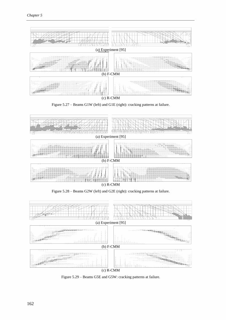
Chapter 5

162

(a) Experiment [95]

(b) F-CMM

(c) R-CMM

Figure 5.27 – Beams G1W (left) and G1E (right): cracking patterns at failure.

(a) Experiment [95]

(b) F-CMM

(c) R-CMM

Figure 5.28 – Beams G2W (left) and G2E (right): cracking patterns at failure.

(a) Experiment [95]

(b) F-CMM

(c) R-CMM

Figure 5.29 – Beams G5E and G5W: cracking patterns at failure.


163

0

30

60

90

0 8Distance from the support [m]

Cra

ck a

ng

le [

deg

]

F-CMM

R-CMM

Exp.

G1W

0

30

60

90

08Distance from the support [m]

Cra

ck a

ng

le [

deg

]

F-CMMR-CMMExp.

G1E

0

30

60

90


Cra

ck a

ng

le [

deg

]

F-CMM

R-CMM

Exp.

G2W

0

30

60

90


Cra

ck a

ng

le [

deg

]

F-CMM

R-CMM

Exp.

G2E

0

30

60

90


Cra

ck a

ng

le [

deg

]

F-CMM

R-CMM

Exp.

G5W

0

30

60

90


Cra

ck a

ng

le [

deg

]

F-CMM

R-CMM

Exp.

G5E

Figure 5.30 – Web crack angles for specimens G1, G2 and G5.

Table 5.8 – Measured and calculated average spacing of the web shear cracks

Girder

Average web shear crack spacing [mm]

Measured F-CMM R-CMM

G1E 148 140 140

G1W 94 140 140

G2E 130 111 109

G2W 106 112 110

G5E 144 150 150

G5W 154 150 150

Chapter 5

164

5.5 Analysis of the deformation capacity of plastic hinges with

high shear stresses


The experiments in this test series aimed at investigating the influence of some major

parameters on the deformation capacity of conventionally reinforced and prestressed

concrete girders [218]. In particular, the tests were planned to study the development of

plastic hinges in regions subjected to high bending moments and shear forces using large

scale specimens. Although a total of six girders were tested (T1 to T6), here only three

girders will be analysed (T1, T2 and T4).

The girders are simply supported and have an overhang on one side (Figure 5.31). Each

girder was subjected to a single load at the free end of the overhang and a uniformly

distributed load in the span between the supports. In a first phase, the specimens were

subjected to proportionally increasing loads with Q = 1.6∙P. After onset of yielding of the

longitudinal reinforcement in the negative moment region (over support B) the vertical

displacement at the free end of the overhang was blocked and the distributed force Q was

increased until failure. In the second phase the girders become statically indeterminate.

(a)

(b)

Figure 5.31 – Geometry and reinforcement content of the analysed girders.


165

The specimens T1, T2 and T4 have the same amount of longitudinal reinforcement in the

critical regions, see Figure 5.31. Therefore, the theoretical bending mechanism with two

plastic hinges leads to the same collapse load in all the three girders. The dimensioning of

the shear reinforcement was made assuming a discontinuous stress field with different

inclinations of the diagonal compressive struts. As can be seen in Figure 5.31 (b), this leads

to significantly different amounts of stirrups in girders T2/T4 when compared to girder T1.

The longitudinal reinforcement of beams T1 and T2 was curtailed according to the tension

chord forces given by the corresponding discontinuous stress field. The longitudinal

reinforcement in specimen T4 was not curtailed. For details regarding the reinforcement

layout refer to the test report [218]. The concrete strength equals cf 46.5, 48.4 and

45.8MPa for beams T1, T2 and T4, respectively. The steel properties are summarized in

Table 5.9 and the adopted finite element mesh is depicted in Figure 5.32.

Table 5.9 – Steel properties

Rebar Ø10

Ø12 Ø14 Ø20 Ø22 Ø26

fsy

[MPa] 506 498 482 502 563 511

fsu

[MPa] 634 624 616 635 744 633

su

[‰] 129 144 132 128 105 139

(a) Phase 1

(b) Phase 2

Figure 5.32 – Finite element mesh of girder T2.

The calculation of the rotation capacity of plastic hinges is highly dependent on the correct

definition of the concrete ductility in the compressed flanges. In this case, concrete in the

bottom flange of the overhang is confined by closely spaced stirrups and hoops, as

Chapter 5

166

depicted in Figure 5.31. This confinement introduces a three-dimensional stress state

responsible for both strength and ductility increase of the compressed concrete which

cannot be directly modelled using a plane stress formulation. In the present work, a rational

procedure was adopted for incorporating this three-dimensional behaviour into the

constitutive laws, following the lines of the Compression Chord Model1 (CCM) proposed

by Sigrist [218]. The confined compressive strength is given by expression (2.23), where

the confining stresses are assumed to be mobilized by yielding of the transversal

reinforcement. Taking into account the fact that the confinement is provided at discrete

locations spaced of sc, see Figure 5.33 (a), the average confined concrete strength is given

by

c

c

c

c

sccb

s

a

sff 11413 (5.1)

where the mechanical reinforcement ratio s is given by (see Figure 5.33 (a) for notation):

zys ;min

ccc

sysz

z

ccc

sysy

yfsb

fA

fsa

fA

;

(5.2)

0

60

0 0.02 / L d

c

[MPa]

Confined

Unconfined

L d ≈ 0.30 m

(a) (b)

Figure 5.33 – Compression chord model: (a) notation; (b) comparison between the confined an unconfined

stress-strain diagrams for the bottom flange of beam T1.

The strain at peak stress is calculated from:

1 Translated from the German Druckgurtmodell.


167

45 3

03

c

c

cf

f (5.3)

As discussed in 2.4.2, with increasing confinement the post-peak branch of the concrete

stress-strain curve experiences a gradual transition from softening to ductile behaviour. In

the post-peak regime, it is assumed in the CCM that the deformations localize along a

length Ld = 2∙ac (with ac ≤ bc). The displacement 50 corresponding to a post peak stress

equal to 0.5∙fc3 is here conservatively estimated from:

c

c

zyc

d a

s

L 211.03

50

(5.4)

Although this procedure can be automated, in the present formulation the user must define

a modified compressive fracture energy GC that fits the post-peak strains given by (5.4).

The adopted stress-strain curves for confined and unconfined concrete are compared in

Figure 5.33 (b) for the case of the bottom flange of girder T1. Objectivity of the results

with respect to the finite element size is guaranteed by performing the regularization of the

post-peak branch along the lines of the crack band model. It is remarked that the effect of

cover spalling due to buckling of the longitudinal reinforcement is not included in the

formulation.

5.5.2 Results


Girder T1 failed by crushing of the bottom flange after the formation of two plastic hinges

in the regions of maximum bending moments. This can be considered a bending failure

motivated by the exhaustion of the rotation capacity of the plastic hinge over the support

region. Girders T2 and T4 experienced a web crushing failure in a typical discontinuity

region. However, girder T2 exhibited a yielding plateau in the force-displacement curve,

whereas girder T4 experienced a brittle failure. The failure loads and failure modes are

summarized in Table 5.10. According to the Eurocode 2 variable angle truss model, girder

T1 is not shear critical while girders T2 and T4 are shear critical and do not achieve the

failure load corresponding to the bending mechanism.

Chapter 5

168



Qu

[kN] Mode

(1) Qu

[kN] Mode

(1) Rat.

(2)

Qu

[kN] Mode

(1) Rat.

(2)

Qu

[kN] Mode

(3) Rat.

(2)

T1 1892 FC 1939 FC 0.98 1945 FC 0.97 1893 B 1.00

T2 1805 WC 1774 WC 1.02 1763 WC 1.02 1825 C/S 0.99

T4 1716 WC 1752 WC 0.98 1762 WC 0.97 1759 C/S 0.98

(1) Failure mode: FC – bottom flange compressive failure; WC – web crushing failure

(2) Failure load ratio: Qu,exp / Qu,calculated

(3) Failure mode according to the EC2 variable angle truss model: S – failure governed by the stirrups; C –

failure governed by crushing of the web; B – Bending failure with two plastic hinges.

The pictures of the failure region and the contour levels of the state variable Emax at peak

load are presented in Figure 5.34 through Figure 5.36. It can be seen that both models

correctly reproduce the observed failure modes. However, and as previously noticed,

crushing of the web concrete tends to appear localized in the finite elements close to the

compressed flange. In these cases, failure was initiated by crushing of the web concrete in

the vicinities of the support, which seems to be consistent with the experimental failure

mode.

(a)

(b)

Figure 5.34 – Girder T1 at failure: (a) detail of the failure region; (b) Emax contour levels in the post-peak stage

for the F-CMM (top) and R-CMM (bottom).


169

(a)

(b)



(a)

(b)




The force deformation curves are depicted in Figure 5.37. Regarding specimen T1, which

failed with the formation of the two plastic hinges, a good estimate of the deformation

capacity could be obtained, thus validating the procedure described above for taking into

account the confinement provided to the bottom flange concrete in the region of the

continuous support. The ultimate deformation of girder T2 is clearly underestimated. In the

Chapter 5

170

numerical analysis, failure occurs shortly after longitudinal steel yielding in the span and

no yielding plateau could be obtained. Nonetheless, the brittle behaviour of girder T4 is

accurately reproduced. It is recalled that these beams contained the same amount of

stirrups and that T2 had curtailed reinforcement. Considering the fact the concrete strength

of girder T2 was only marginally higher than that of girder T4, it can be concluded that the

delayed crushing of the web concrete in girder T2 with respect to that of girder T4 can be

explained by the inherent scatter of the cracked concrete compressive strength.

0

2000

0 200 1 [mm]

Q [

kN

]

Exp.

F-CMM

R-CMM

LS1

LS2

LS3

LS4

LS5

Peak loadT1

0

2000

0 200 1 [mm]

Q [

kN

]

Exp.

F-CMM

R-CMM

LS1

LS2

LS3

LS4

LS5

Peak loadT2

0

2000

0 200 1 [mm]

Q [

kN

]

Exp.

F-CMM

R-CMM

LS1

LS2

LS3

LS4

LS5

Peak loadT4

Figure 5.37 – Force-deformation curves for beams T1, T2 and T4.

The longitudinal strains obtained by measuring the relative displacements of targets

located in the top and bottom fibres of beam T1, as well as the corresponding curvature

distribution along the beam longitudinal axis, are presented in Figure 5.38. A good match

with the numerical values is observed, namely in what concerns the length of the plastic

hinges, which is an important feature in order to get accurate estimates of its rotation

capacity. The results correspond to a loading step where the displacement at the span

equals 1 = 95mm (approximately half-way through the yielding plateau observed in

Figure 5.37).

-5

0

5

10

15

20

25

-3 0 3 6 9

x [m]

xx

[x10

3]

F-CMM

Exp. (Bottom)

Exp. (Top)

T1

-10

0

10

20

-3 0 3 6 9

x [m]

Cu

rvat

ure

[x

10

3]

F-CMM

Exp.

T1

Figure 5.38 – Average longitudinal strains (left) and curvatures (right) for beam T1 corresponding to a

vertical displacement in the span of 1 = 95mm.


171


The observed and calculated cracking patterns at failure are depicted in Figure 5.39 trough

Figure 5.41. Once again the calculated cracking patterns provide a good picture of the real

cracking pattern.


(b) F-CMM

(c) R-CMM

Figure 5.39 – Beam T1: cracking patterns at failure.


(b) F-CMM

(c) R-CMM



(b) F-CMM

(c) R-CMM


Chapter 5

172


A validation campaign was undertaken using a set of experimental tests on large scale

shear critical structural elements. Both continuity and discontinuity regions were analysed.

The models proved capable of reproducing shear failures in demanding situations, such as

the ones involving plastic strains in the longitudinal reinforcement. The effect of normal

forces on the shear behaviour was dully modelled. Although both the rotating and fixed

crack models performed well, the F-CMM provided better estimates of the failure modes,

failure loads and cracking patterns. The implementation of both models proved robust and

the force-deformation responses could be computed in the post-peak range, thus allowing a

clear identification of the failure mechanisms. When compared to the Eurocode 2

provisions based on the variable angle truss model, the numerical analysis allowed a

significant improvement in the estimates of shear failure load of beams containing low

amounts of shear reinforcement. Although the focus was driven to the modelling of the

shear failures in shear reinforced concrete girders, an example was presented of a concrete

girder failing in bending. In this case, both models allowed good estimates of the

deformation capacity and an accurate sizing of the plastic hinge regions.

In spite of the overall good results, some limitations were found. (1) Although not severe,

the deformation capacity of the stirrups is somewhat underestimated whenever failure is

governed by stirrup rupture. This can be attributed to the fact that the model cannot

reproduce bond slip occurring across several cracks; (2) Despite the fact that the F-CMM

can reproduce the associated crack kinematics, the shear sliding failure mode that occurred

in girders MVN2 and MVN3 could not be clearly evidenced due to anticipated crushing of

web concrete. It seems that the adopted softening law, which is based on the results

obtained on RC panels, gives somewhat conservative estimates of the effective

compressive strength in discontinuity regions. Nonetheless, the failure loads and the force-

deformations curves were still in good agreement with the observed ones and the failure

region is correctly identified; (3) Finally, due to the kinematic description of the

displacement field based on the concept of weak discontinuities, web crushing failure is

systematically localized along a row of finite elements instead of spreading throughout the

whole web. Although this effect has almost no implications in the calculation of the peak

load, it may influence the computation of the load carrying mechanisms in the post-peak

regime. The well-posedness recovery using a regularization of the compressive strain field

based on a non-local approach might be a possible remedy for this situation.

173

6 Simplified models for engineering practice

6.1 General

In the previous chapters a numerical model was developed for NLFEA of structural

concrete elements allowing detailed examinations of the structural behaviour. Besides

enabling the determination of the complete force-deformation curves, also cracking

patterns and crack widths can be estimated with good accuracy. However, in the course of

a structural examination of an existing bridge such a detailed structural analysis may not

always be required. Even if this is not the case, in early stages of the structural assessment

simpler methods should be employed to provide a first estimate of the determinant failure

modes and corresponding failure loads. The advantage of a stepwise procedure in the

safety evaluation of existing structures is widely recognized [36; 66; 259] and has been

adopted in the recent fib model code [87]. However, it is also important that the successive

methods are somehow related. The simpler methods should preferably be based on the

more detailed ones through transparent simplifying assumptions in order to keep clarity

and consistency between the results obtained in the successive levels of analysis. In the

present chapter the focus is driven on the shear strength assessment of structural elements

containing at least the minimal amount of shear reinforcement and plasticity theory

concepts are adopted in the formulation of simplified models. It is shown how plasticity

based structural analysis methods relate to the models developed in the previous chapters

and how those can be used in intermediate stages of assessment.

Based on the equilibrium equations of the cracked membrane element and on the work of

Kaufmann [117; 118], considering the simplifying assumptions mentioned in Section 3.4

and the constitutive equation (3.24) for the effective concrete compressive strength fc,ef, in

Section 6.2 a simplified analytical model is derived for shear strength assessment of RC

panels which can be considered as an extension of the classical limit analysis equations.

This formulation is then used at the structural level for obtaining continuous stress fields at

failure conditions through a simplified nonlinear analysis model. It is also shown how the

same set of equations can be used for the strength assessment of general structural concrete

Chapter 6

174

elements using discontinuous stress fields, thus establishing a link between the developed

NLFEA models and the analytical engineering methods of limit analysis for structural

concrete elements. Finally, in Section 6.3 a sectional analysis method is developed for

continuity (or B-) regions which results in a set of expressions similar to those of the well

known variable angle truss model. The proposed model can be used in an intermediate

assessment stage and has the advantage of being formally similar to the shear design

provisions used in the recent European codes of practice.

6.2 Limit analysis methods for structural concrete elements

subjected to in-plane forces

6.2.1 Overview and general considerations

Limit analysis methods result from the application of the theory of plasticity to structural

concrete, allowing a unified treatment of the design methods of beams, walls, slabs and

shells [150; 163; 169]. Concrete and steel are treated as rigid-plastic materials and

therefore only ultimate loads can be calculated. These methods have been built on a sound

physical basis through the establishment of the lower-bound (or static) and upper-bound

(or kinematic) theorems of limit analysis.

The lower-bound theorem states that any load corresponding to a statically admissible state

of stress everywhere at, or bellow, yield is not higher than the ultimate load. Therefore, in

the lower-bound methods an internal force flow in equilibrium with the external loads is

assumed. This admissible stress field can be idealized as a discontinuous stress field [146;

147; 149; 167; 169; 217], or simply as a system of struts and ties [149; 208; 209] in which

the stresses are replaced by its static equivalent resultants – a strut and tie model can be

regarded as a discrete representation of the associated discontinuous stress field. While

these methods are applicable to general geometric and loading configurations, simple

section-by-section analysis procedures can be derived for linear members – beams and

columns – in which all static and geometric quantities vary only gradually along the

structural axis. The shear design method based on the variable angle truss model proposed

in the Eurocode 2 [46] is an example of such an analysis procedure.

The lower bound methods are powerful analysis and design tools that permit visualising

the force flow throughout the structure, allowing for consistent dimensioning and detailing.

Simplified models for engineering practice

175

However, a certain degree of expertise is necessary for the application of these methods in

cases of structures with complex geometry since the choice of an appropriate stress field

may not be straightforward. In these cases, rather than determining the reinforcement from

a discontinuous stress field solution, admissible stress fields can be obtained from linear

elastic finite element analysis. The yield conditions for membrane elements [168; 169]

allow dimensioning the reinforcement in such cases [134]. Although this may have the

advantage of restoring uniqueness to the problem, the resulting reinforcement layouts can

be inadequate for practical use. Moreover, in the evaluation of an existing structure this

procedure can be too conservative since the adoption of a linear elastic stress field is

incoherent with the assumed plastic behaviour and may deviate considerably from the

actual stress field at failure conditions. Consistent admissible continuous stress fields can

still be established with the aid of the finite element method by using appropriate

elastic-plastic constitutive relationships [79]. Good agreement with experimental findings

has been reported [80] and this method is suitable for refined checks of a previous design

or of an existing structure.

The upper-bound methods are also suited for checking a previous design or an existing

structure. These methods involve the consideration of an admissible failure mechanism and

the determination of the corresponding work W done by the external forces, as well as the

internal energy dissipation D at lines of kinematic discontinuity [100; 149; 169; 217]. The

failure load corresponding to a given mechanism is determined from condition W = D. The

upper-bound theorem states that any load resulting from the consideration of a

kinematically admissible state of deformation is not lower than the ultimate load.

Therefore, the most critical mechanism is the one providing the lowest failure load and can

be found either through a minimization procedure or by trial and error considering a

discrete number of admissible failure mechanisms.

As concrete is a strain softening and brittle material, its idealization as a perfectly plastic

material can be debatable. However, this limited material ductility can be taken into

account by choosing an appropriate reduced value for the effective concrete compressive

strength fc,ef. The analysis and design with limit analysis methods also requires a certain

amount of structural ductility enabling the mobilization of the assumed admissible stress

field or failure mechanism. In general, in order to guarantee the required structural ductility,

besides a suitable value for the concrete compressive strength, these methods should be

applied in conjunction with a well distributed minimum reinforcement in the regions where

no main reinforcement is required. As the compatibility conditions are not explicitly

Chapter 6

176

verified, design codes usually limit the inclination of the compressive stress field so that

the plastic stress field is not so far off from the elastic solution. This limitation is also

imposed to avoid failures governed by steel rupture, excessive softening of concrete or

sliding through a dominant crack. Rooted on the models developed in Chapter 3 and

following the work of Kaufmann [117], a different approach is proposed in this chapter,

whereby the limits to the inclination of the compression field are removed and replaced by

rationally derived expressions based on a simplified strain compatibility analysis.

6.2.2 Yield conditions of reinforced concrete membranes

The yield conditions for RC membranes under in-plane stress conditions can be derived to

determine its load carrying capacity according to the lower-bound theorem of limit analysis.

Reinforced concrete is treated as a composite material containing concrete and reinforcing

bars, both considered as rigid-plastic materials. Concrete is assumed to obey the modified

Coulomb criterion with zero tensile cut-off [169], that is, the tensile strength is neglected.

In plane stress conditions, this criterion corresponds to two conical surfaces described by

the equations yxxy 2 and yefcxefcxy ff ,,

2 . In the principal stress space

21, the criterion comes down to the square yield locus defined by the vertices (0,0),

(0,- fc,ef),(- fc,ef,- fc,ef), (-fc,ef, 0).

In the present work, and according to what has been exposed in Chapters 2 and 3, the

effective compressive strength efcf , is considered proportional to3/2

cf . This being the case,

the mechanical reinforcement ratios in the x- and y- directions are defined as:

32

,

c

xxsyx

xf

f

32

,

c

yysyy

yf

f

(6.1)

Although formal derivations can be made starting from the basic assumptions of plasticity

theory, the yield condition for RC membranes can be easily derived from the simplified

form of the general equilibrium equations given by (3.16). Using the notation above and

defining

3/13/2

, / cfecefc fff (6.2)

the yield conditions and the corresponding angle can be expressed in the following form:


177

yx

c

xy

fY

3/21 :

y

x

tan

yy

c

xy

fY

3/22 :

y

y

tan

xx

c

xy

fY

3/23 :

x

x

tan

2

:3/24

c

xy

fY 1tan

(6.3)

In the precedent expressions, the yield conditions Y1 to Y4 correspond to the four failure

modes that can be distinguished in limit analysis, respectively: (1) x- and y-reinforcement

yielding; (2) concrete crushing with elastic x-reinforcement; (3) concrete crushing with

elastic y-reinforcement; and (4) concrete crushing with both reinforcements in the elastic

range.

0

2.5

0 2.5 x

y

1

2

41

2

34

sr,y = f sy,y

sr,x = f sy,xtan = 0.4

tan = 2.5

0

1.3

0 2.5 y

Series1

Series3

Series4

Series6

Series2

Series5

Series7

xy,u

f c2/3

x >1.6

x = 0.45

tan = 2.5

x = 1.0

(a) (b)

Figure 6.1 – Limit analysis. Comparison with experimental results: (a) failure modes; (b) shear strength.

Muttoni [163; 167] proposed to use =1.6 to calculate the effective concrete strength

under moderate transverse strains, and therefore3/2

, 6.1 cefc ff . If fc0 = 20MPa is taken in

Eq. (6.2), this is equivalent to considering e ≈ 0.6. With this constant value for fc,ef, the

predicted boundaries of the 4 failure regimes are depicted in Figure 6.1(a) together with the

experimental failure modes of the same set of 54 RC panels introduced in Chapter 3. The

thin dashed lines correspond to the limitation that is imposed in the Eurocode 2 [46], per

Chapter 6

178

example, regarding the maximum inclination of the diagonal compressive field. Two

sections of the failure surface are presented in Figure 6.1(b). Although the shear strength of

the panels can be fairly predicted, the agreement between calculated and experimental

failure modes is rather poor. In limit analysis, shear failures due to sliding across wide

open cracks, or stirrup rupture due to exhaustion of the steel deformation capacity must

also be included in the web crushing failure mode. Since an overestimation of the shear

strength of panels lightly reinforced in the y- direction and failing in regime 2 is obtained

with e ≈ 0.6, some kind of limitation to angle is essential if a constant value for is

adopted.

6.2.3 Yield conditions accounting for compression softening

6.2.3.1 Formulation

A further improvement on limit analysis methods was made by Kaufmann [117] by

incorporating the softened compressive strength relationship (3.24) into the yield

conditions for membrane elements, thereby eliminating the need for ad hoc upper limits to

tan

From the Mohr circle of strains it is possible to show that:

2

21 tan)( xx (6.4)

The inclusion of the softened compressive strength into the yield conditions of regimes 2, 3

and 4 can be achieved making two additional assumptions: (1) when concrete crushes the

principal compressive average strain is 002.02 ; (2) a conservative estimate of the

softening coefficient can be made considering that the non-yielding reinforcements are

about to yield, which results in an average strain approximately given by

syxsyyx Ef /8.0 /,/ ≈ 0.002. In these circumstances the strain softening coefficient of

Eq. (3.24) simplifies to

2tan326.0248.1

1

e (6.5)

where the parameter Cm, see Eq. (3.24), was taken as 1.0 for consistency with the remarks

made in 3.6.1 regarding the effects of the explicit modelling of crack shear slip in the

softening coefficient. Noting that tan is given by Eqs. (6.3) in each of the four failure


179

regimes, and after some algebraic manipulation, the yield conditions can be expressed in

the following form:

yx

c

xy

fY

3/21 :

y

x

tan

tan:3/22 y

c

xy

fY

y

cf

3/1

007.30.2417.2tan

3/1

03/24 318.0: c

c

xyf

fY

1tan

(6.6)

0

2.5

0 2.5 x

y

1

2

41

2

3 4

sr,y = f sy,y

sr,x = f sy,x

0

1.3

0 2.5 y

Series1

Series3

Series4

Series5

Series7

xy,u

f c2/3

x >1

x = 0.45

(a) (b)

0

1.25

0 1.25 xy,u / f c2/3

xy,u / f c2/3

1

2

4

calc

exp

Limit

analysis

+10%

-10%

(c)

Figure 6.2 – Limit analysis accounting for compression softening. Comparison with experimental results:

(a) failure modes; (b) and (c) shear strength.

Chapter 6

180

The expression for yield condition Y3 can be obtained from Y2 by exchanging indexes and

by using ‘ = 90 – instead of The predicted boundaries of the 4 failure regimes are

depicted in Figure 6.2 (a) together with the experimental failure modes of the same 54 RC

panels that were already used in Chapter 3. In Figure 6.2 (b) the theoretical failure surface

is compared to the experimental shear strengths of panels with x ≈ 0.45 and x > 1. Good

agreement can be found, demonstrating the suitability of this formulation for the design,

capacity evaluation and identification of the mode of failure of RC membrane elements. A

summary of the results of the validation campaign is presented in Table 3.3 and in Figure

6.2 (c). The average value of the calcuu ,exp, ratio is 1.10 and the coefficient of variation

equals 14.7%. A value of fc0 = 20MPa was adopted in the calculations.

6.2.3.2 Comparison to the R-CMM and F-CMM

It is interesting to confirm that the precision level increases with the complexity of the

model. As should be expected, the data summarized in Table 3.3 reveals that the dispersion

of the exp,, ucalcu ratio obtained with the limit analysis formulation accounting for

compression softening is somewhat larger than the obtained with the F-CMM or R-CMM.

However, by not considering the hardening behaviour of reinforcement steel and by

adopting conservative estimates of the compression softening coefficient, the limit analysis

formulation is generally on the safe side when compared to the previously mentioned

models, even in the cases of failure due to transverse steel rupture or due to sliding along

the shear cracks (the latter can only be predicted by the F-CMM). This can be confirmed in

the failure envelope sections depicted in Figure 6.3. It can thus be concluded that the limit

analysis formulation accounting for compression softening is a suitable method for a

stepwise procedure for the shear safety assessment of existing structures culminating, if

necessary, with a nonlinear analysis using the models developed in Chapters 3 and 4.


181

0

0.35

0 0.35

R-CMM

F-CMM

Limit analysis

xy,u

f c

y f sy

f c

x = y

R-CMM

= 1

F-CMM

, = 1

, = 1

( x = y )

0

0.35

0 0.35

R-CMM

F-CMM

Series2

xy,u

f c

y f sy

f c

x = 0.57%

R-CMM

= 1

F-CMM

, = 1

, = 1

( x = 0.20)

0

0.35

0 0.35

R-CMM, l=1

F-CMM

Limit Analysis

xy,u

f c

y f sy

f c

x = 1.7% = 1

( x = 0.60)

0

0.35

0 0.35

R-CMM, l=1

F-CMM

Limit Analysis

xy,u

f c

y f sy

f c

x = 2.8%

( x = 1.00)

Figure 6.3 – Sections of the F-CMM, R-CMM and limit analysis with compression softening failure

envelopes. Calculations were made using: cf 45 MPa, syf 450 MPa, suf 580 MPa, su 50‰

and Ø = 16mm.

6.2.3.3 Effect of the strains in the stronger reinforcement

The yield conditions (6.6) were derived assuming x = 0.002, which is equivalent to

assuming that the stronger reinforcement is about to yield. In some cases this assumption

can be inadequate: in prestressed concrete structures longitudinal strains below the yielding

strain can usually be found in shear critical regions; on the other hand, in statically

indeterminate structures, notably in the hogging moment region of continuous beams,

plastic reinforcement strains can be found in shear critical zones. In these circumstances, a

refined shear strength assessment can be made using the equations (6.7) where the

condition x = 0.002 was removed:

Chapter 6

182

tan:3/22 y

c

xy

fY

x

x

y

cx

f

6012.0

002.021.44

1156.06046.0

tan

3/1

0

x

c

c

xy f

fY

7.325497.2:

3/1

0

3/24

1tan

(6.7)

0

1.3

0 1.3 y

xy,u

f '2/3

c

ς ( 1), x = 0.002

ς = 0.55

ς = 0.60

ς ( 1), x = 0.001

ς ( 1), x = 0

f c 0 = 20MPa

0

3.5

0 1.3 y

tan ς e ( 1), x = 0

ς e ( 1), x = 0.002

ς e = 0.55

ς e ( 1), x = 0.001

ς e = 0.60

f c 0 = 20MPa

(a) (b)

0

1

1 3.5tan

ς e ( 1), x = 0

ς e ( 1), x = 0.002

ς e = 0.55

ς e ( 1), x = 0.001

ς e = 0.60

ς e

tan = 2.5

0

1

1 3.5tan

ς e ( 1), x = 0

ς e ( 1), x = 0.002

ς e = 0.55

ς e ( 1), x = 0.001

ς e = 0.60

f c 0 = 20MPa

ς e

tan = 2.5

(c)

Figure 6.4 –Limit analysis: (a) sections to the failure envelope; (b) evolution of tan with the mechanical

reinforcement ratio y; (c) relation between the strain softening coefficient e and tan. The amount of

stronger reinforcement is such that failure occurs in the regimes 2 and 4.


183

The failure envelope sections and the corresponding values of tan are depicted in Figure

6.4 and compared to the results obtained with traditional limit analysis considering

constant fc,ef. In the latter, the limitation tan ≤ 2.5 was considered. According to Eq. (6.1),

and for very low amounts of vertical reinforcement, tan can assume values up to 3.5.

Beyond this limit it is likely that the minimum vertical steel requirements govern, and limit

analysis methods cease to be applicable, as discussed in Section 6.2.1. The relation

between the softening coefficient e and tan is also presented in the figure and a

comparison can be made with the constant values e =0.55…0.60 adopted when the

influence of 1 is not explicitly taken into account.

6.2.4 Continuous stress fields

The equilibrium equations (3.16) used in the development of the yield conditions can be

implemented in a finite element code following the same formalism adopted in the

implementation of the R-CMM. This offers the possibility of migration from the

membrane level - in which a uniform state of equilibrium is assumed - to the structural

level of analysis. The previously derived expressions can be then applied in the automatic

generation of stress fields expressing the stress flow at failure conditions of structural

concrete elements. The stress fields obtained through the procedure described in this

section are designated as continuous in opposition to the traditional discontinuous stress

fields, see Section 6.2.5.

6.2.4.1 Constitutive laws

Simple constitutive laws are adopted here, observing more closely limit analysis

assumptions and current engineering practice than in the case of the detailed models

developed in Chapters 3 and 4. An elastic-perfectly plastic stress-strain law is adopted both

for concrete and the reinforcements. Likewise the yield conditions accounting for

compression softening, the compressive strength of cracked concrete is reduced according

to Eq. (3.24). The biaxial compression effects are disregarded and the square yield locus

mentioned in Section 6.2.2 is adopted. The simplified constitutive laws are summarized in

Figure 6.5.

Since bond effects and concrete tensile strength are neglected, the deformations are in

general overestimated. If accurate load-deformation curves are of interest, the F-CMM or

the R-CMM models should be used. However, if only an estimate of the ultimate load is of

interest, this simplified formulation can be most useful, namely due its close relation to

Chapter 6

184

limit analysis methods. Moreover, the required input variables reduce to the concrete

strength and steel yielding stress, which is quite adequate for a simplified model.

(a) (b) (c)

0

1

0 100

zf

f 'c [MPa]

0

1

0 20

ze

1 [x103]

(d)

Figure 6.5 –Continuous stress field analysis: (a) Yield criterion; (b) and (c) Elastic-plastic constitutive

laws; (d) Softened compressive strength

6.2.4.2 Examples

Shear in continuity regions – Beams VN2 and VN4 tested by Kaufmann and Marti [119]

These beams have already been analysed in the previous chapter and represent a typical

situation where shear failure occurs in a continuity region, that is, away from stress

disturbances caused by the introduction of point loads. They are here re-analysed using the

simplified model described above.

In the case of beam VN2, the calculated shear strength is Vu,cal = 505 kN, leading to the

ratio Vu,exp/Vu,cal = 1.09. The struts are computed to be 19.4º inclined with respect to the

horizontal axis, which is equivalent to consider tan = 2.84, and concrete crushes for

fc,ef = 16.4MPa. The stress field at failure is depicted in Figure 6.6. In the contour levels

with the compressive stresses at failure, an inclined parallel stress band with compressive

stresses bellow -16MPa is clearly identified, as expected in a B-region subjected to

130 3

1

c

ff

18108.1

1

e

cfeefc ff ,


185

constant shear force. Stirrups are yielding through the entire length of the web. The

computed stress field gives a clear indication of the force flow in the structural element.

In the case of beam VN4, the calculated shear strength is Vu,cal = 537 kN, leading to the

ratio Vu,exp/Vu,cal = 1.05. The struts are computed to be 18.5º inclined with respect to the

horizontal axis, which is equivalent to consider tan = 2.98, and concrete crushes for fc,ef =

18.2MPa. The stress field is very similar to that obtained for beam VN2, and is not

presented here.

(a) Stress field at failure

(b) Compressive stress contours at failure

(c) Stirrups stresses at failure

Figure 6.6 – Continuous stress field analysis of beam VN2.

As expected in a lower bound solution, the computed failure loads in both specimens are

on the safe side. Nevertheless, only a minor decrease in accuracy is obtained compared to

the results presented in Chapter 5.

Shear in discontinuity regions - Beams G2E and G5W tested by Kuchma et al. [94; 127]

As examples of shear failures occurring in a typical discontinuity region, the beams G2E

and G5W (see Chapter 5) were selected for analysis. The stirrup ratios equal w = 0.94 and

0.18% respectively.

In the continuous stress field analysis, both beams failed with local crushing of the

concrete in the web immediately above the support. The ultimate loads were qu = 435 and

235kN/m for G2E and G5W, respectively, which leads to qu,exp/qu,cal ratios of 1.23 and 1.13.

The computed stress fields are depicted in Figure 6.7. Compressive stresses close to the

effective compressive strength are only obtained in a localized region above the support,

Chapter 6

186

providing clear evidence that failure is governed by local conditions at the ends of the

specimens. Although stirrup yielding is computed for both beams, in the case of G2E, the

yielding zone is very limited.

(a) Experiment

(b) Stress field at failure

(c) Principal compressive strains (2 < -0.002 means concrete crushing)

(d) Stirrup stresses (red areas indicate yielding zones)

Figure 6.7 – Continuous stress field analysis of beams G5W (left) and G2E (right).

The computed stress fields provide useful information about the stress flow and the

identification of the critical zone. As expected, lower bound estimates of the failure load

were again calculated. The continuous stress field analysis results deviate more from those

obtained in the previous chapter in the case of the beam with the lowest amount of stirrups.

In this case, tensile stresses in between the cracks and the post yielding behaviour of

reinforcing steel have a more important contribution for the load carrying capacity.

6.2.5 Discontinuous stress fields

6.2.5.1 Basic concepts

Within the framework of the theory of plasticity, discontinuous stress fields offer the

possibility of migrating from the membrane element level to the structural level of analysis

without using finite element techniques to solve the boundary value problem. A given

discontinuous stress field solution represents one statically admissible stress field, which in

light of the lower-bound theorem of limit analysis represents a solution on the safe side as

long as an appropriate value for the effective concrete compressive strength is chosen.


187

As schematically depicted in Figure 6.8, lines of stress discontinuity are assumed in virtue

of the underlying rigid-plastic material behaviour. It can be shown [169] that the

satisfaction of the equilibrium equations implies the continuity of the shear stress ntI = nt

II

and of the normal stress nI = n

II, where the local n-t axes are defined normal and

tangential to the discontinuity line, respectively. However, no claims for the sake of

equilibrium are made regarding the axial stress parallel (or tangential) to the discontinuity

linet. Therefore, only axial stresses acting parallel to the discontinuity line may exhibit a

jump across the stress discontinuity.

(a) (b)

Figure 6.8 – Stress discontinuity lines: (a) notation; (b) discontinuous stress field for direct strut action.

Although more general stress fields can be derived, in practice it is convenient to use struts

(Figure 6.8(b)), fans and parallel stress bands as basic stress field components, see Figure

6.9. The state of stress in each of these basic elements has been thoroughly established in

several works, mostly developed at the Swiss Federal Institute of Technology, Zurich, as

per example in references [117; 145; 162; 216; 228].

(a) (b) (c)

Figure 6.9 – Basic discontinuous stress field elements: (a) centred fan with intersection point away from

the chords; (b) parallel stress band; (c) centred fan with intersection point in the bottom chord (note that in

this case the forces in the upper chord have sign opposite to the represented).

Chapter 6

188

Taking once again the simplified form of the equilibrium equations of the cracked

membrane element (3.16), and assuming a membrane element with uniform thickness bw, it

is possible to conclude that

2

2 tan1w

v

cb

q (6.8)

with wv fqq being the resultant vertical force, ywbq the external vertical load and

syyww bf the stirrup force (all these forces per unit length). In the simplest case of the

parallel stress band, the principal compressive stresses in concrete c2 are constant if both

the external load and the stirrup force distributions are uniform. The fans presented in

Figure 6.9 are called centred because the stress trajectories meet in one point. In this case

the concrete stresses vary hyperbolically along the stress trajectories and can still be

calculated with Eq. (6.8), but noting that qv and cease to be constant along the fan [228]:

v

v

swsvdc

acydafqq

,

acydc

acxbcc

v

tan (6.9)

In the expression above, the coordinates x and y define a point in the rectangular coordinate

system represented in Figure 6.9, where all the remaining variables are identified. The

force distribution in the chords can be derived from the translational equilibrium equations

of the infinitesimal strut section represented in Figure 6.10:

tan,inf

iiw qfdx

dF

tan,

sup

sws fqxd

dF

, bcxx

(6.10)

(a) (b)

Figure 6.10 – Equilibrium of forces acting in the top (a) and bottom (b) chords.


189

According to the previous expressions, the chord forces vary linearly along parallel stress

bands since has a constant value and uniform distributions of stirrup and external forces

are usually assumed. In the centred fans the variation is parabolic and can be obtained by

integration of Eqs. (6.10) with proper consideration of Eq. (6.9):

v

iiwldc

acxxcbcqfFxF

2

2 2

,inf,inf

ad

acxxabcqfFxF

v

sswl2

2 2

,sup,sup

(6.11)

The expressions above were derived assuming that the chords are straight and parallel to

the x-axis, see Figure 6.9. More general expressions can be derived for curved chords [228],

which are suited for cases where the stress field is deviated by a curved prestressing tendon.

Figure 6.11 – Non-centred fan with nodal region (a) and detail of the node (b).

Infinitely high compressive stresses result at the centre of the fan depicted in Figure 6.9(c).

In reality supports or loading plates have a finite dimension and more detailed admissible

stress fields can be considered adopting non-centred fans with nodal region, as illustrated

in Figure 6.11. Since a reasonable approximation of the stresses in the vicinity of the chord

opposite to the node can be obtained with the centred fan, the non-centred fan can be used

mainly for checking the state of stress in the vicinity of concentrated loads. The equation

describing the boundary of the nodal region can be determined assuming that concrete is

yielding in biaxial compression – that is, the concrete stresses along lines AB, AC and BC

equal fc,ef – and solving the differential equation of equilibrium for the vertical forces. For

constant fc,ef and bw it can be shown [217] that the boundary line is hyperbolic and that

Chapter 6

190

wefc

sws

bf

afqc

,

,

v

nd

ccbah

2

2 (6.12)

which allows checking the minimum node dimensions. The expressions above are valid for

flanged or hollow-box beams in which the flange regions adjacent to the web are assumed

to carry the compressive chord forces. For details refer to [118; 217].

6.2.5.2 The effective compressive strength

As thoroughly discussed in Chapter 3, the effective concrete compressive strength fc,ef can

be conveniently expressed by Eq. (3.24). When a constant value for the softening

coefficient e is adopted, the best fit to the shear strength of RC panels is obtained with

fc0 = 20MPa and e =0.6, as shown in Section 6.2.2. However, for structural concrete

elements other than uniformly stressed RC panels, the results from the numerical analyses

of Chapter 5 show that better agreement between the calculated and observed shear

strength is obtained using fc0 = 30MPa. This fact was attributed to the partial restraint to

laminar splitting provided by the intact concrete surrounding the failure zone, with

particular emphasis on the flanges. This seems to be confirmed in the most recent draft of

the CEB-FIP Model Code 2010 [87] wherein fc,ef is defined similarly to (3.24) with fc0 =

30MPa and e =0.551. The latter is somewhat more conservative, and therefore more

appropriate to be specified in a code, than the best fit value of e =0.6 referred above. Not

surprisingly, it is interesting to confirm that this definition of fc.ef renders practically the

same values in the range 100;0cf (MPa) as the one proposed in the Eurocode 2 [46]

using e =0.6 and f given by (2.20).

As discussed in Section 6.2.3, more accurate shear strength assessments can be made if a

strain compatibility analysis is made such that the dependence of e on the principal

tensile average strains 1 is explicitly taken into account. This is exemplified in the

following examples.

6.2.5.3 Examples

Beams VN2 and VN4 tested by Kaufmann and Marti [119]

The adopted stress field is depicted in Figure 6.12. The similarity with the stress field

obtained using the continuous stress field approach is evident. The critical value of tan is

1 This value of e is proposed for the case of compressive stress fields with the reinforcement running

obliquely to the direction of compression, as is typically the case in the web of a beam.


191

determined in regime 2 using the corresponding Eq. (6.7), for which x and y must be

defined. Since failure occurs in the parallel stress band – note that tan is maximum in this

region – , it is here proposed to use the most unfavourable value of the average

longitudinal strain x occurring in this region, having in mind that the conditioning value

must be located in the web. This corresponds to the locations indicated in the figure, which

yield the same value forx due to the antisymmetric loading conditions. A trial an error

procedure is required since tan depends on x, and the critical location for the

determination of x depends on tan. However, great precision is not necessary in the

determination of x and a couple iterations are usually enough to achieve a reasonable

estimate. For beam VN4 the applied compression force is assumed to be carried

exclusively by the chords.

Figure 6.12 – Discontinuous stress-field for the beams VN2 and VN4.

Defining the lever arm dv = 0.64m as the distance between the centres of the flanges, the

force in the tensile chord can be determined from the bending moment diagram as

FT = M / dv. Knowing the amount of longitudinal steel in the flange As = 106cm2 and

assuming a linear variation of x throughout the cross-section height, the critical average

strain is estimated as:

ss

T

v

v

xEA

F

d

z8.0 (6.13)

where zv is defined in Figure 6.12.

Beam VN2 failed for V = 548kN, which corresponds to extreme bending moments of

M = 548∙5.840/2 = 1600kN.m. Using the appropriate expressions (6.11) the tensile chord

force at the critical location is found to be FT = 1193 kN and the average strain can be

estimated as x = 0.8∙0.55/0.64∙FT / As∙Es = 0.39e-03. Considering f’c = 52.6 MPa, y =

0.122 (see the material properties in Table 5.1) and the estimated value of x, the value

tan = 2.89 is determined from Eq. (6.7). Substituting tan and x in Eq. (3.24), it is

Chapter 6

192

possible to conclude that fc,ef = 16.0MPa. As should be expected, this value is quite close to

that obtained in the continuous stress field analysis. As failure occurs in the parallel stress

band, the corresponding ultimate shear force can be calculated from Eq. (6.8) as Vu,cal =

473 kN, leading to the ratio Vu,exp/Vu,cal = 1.16.

Beam VN4 failed for V = 564kN, corresponding to M = 1647kN.m. Performing

calculations identical to the ones described in the previous paragraph, but noting the

applied compressive force N = 1000kN, it can be found that x = 0.23e-03, tan = 3.04,

fc,ef = 17.6MPa and Vu,cal = 498 kN. This leads to a ratio Vu,exp/Vu,cal = 1.13.

Compared to the failure loads calculated using a constant value for fc,ef, an improvement is

achieved due to the fact that the angle is no longer limited by the condition tan ≤ 2.5.

The failure loads that are obtained with constant fc,ef are identical to the ones calculated

using the Eurocode 2 provisions and are given in Table 5.1. This shows the benefits that

can be gained from performing a more detailed analysis using the proposed procedure.

Moreover, the effects of the compressive axial force could be taken into account. As

should be expected, even better correlation with the experimental failure loads could be

obtained with NLFEA models.

Beam CM2 tested by Cerruti and Marti [53]

Let us consider the beam CM2 tested by Cerruti and Marti [53], see Figure 6.13. Besides

the self weight W, this large scale beam was subjected to a uniform load Q in the span and

to a point load P in the overhang. The test was aimed at verifying the adequacy of the

staggering concept in a specimen with curtailed longitudinal reinforcement. The beam

failed at Q = 1711kN and P = 904.7kN owing to crushing of the web concrete after

extensive yielding of the stirrups in the interior span adjacent to support B. Prior to failure,

yielding of the longitudinal bars in the top and bottom flanges was also observed.

Figure 6.13 –Beam CM2 tested by Cerruti and Marti [53]. Dimensions in mm.


193

One possible discontinuous stress field is presented in Figure 6.14. The lever arm dv was

defined as the distance between the centres of the flanges. The stirrups are uniformly

distributed along the distances indicated in the figure, leading to the provided stirrup forces

fw,r. The stirrup content in the interior span adjacent to support B equals w = 0.895% with

fsy = 457MPa. Considering the compressive strength cf = 44.7MPa, the mechanical

reinforcement ratio y = 0.325 can be calculated.

Figure 6.14 – Stress field analysis of beam CM2.The dashed lines indicate yielding forces provided by the

existing reinforcement.

Admitting in a first iteration that x = 0.002 in the top chord, the value x = 0.675/0.75 =

0.0018 can be calculated in the web immediately bellow the chord. It is recalled that

Chapter 6

194

x = 0.002 already accounts for the tension stiffening effects, being approximately 80% of

the reinforcement yielding strain. Substituting this value in the expression for tan

corresponding to the failure regime 2 given in (6.7), and considering fco = 30MPa, one

obtains tan = 1.81. This angle defines the critical inclination for the fan BON over support

B. The stirrup content is constant in a length of about 1375mm, of which only dv∙tan =

1360mm were mobilized by the fan BNMF. In the adjacent 1388mm segment the spacing

is changed such that w = 0.546 and y = 0.198. Still considering that x = 0.0018 in this

region, the maximum value of tan = 2.17 is determined. Having defined the successive

critical values of tan corresponding to the different segments with uniform stirrup

spacing, the stress field can be constructed. In this case, the critical value of tan is only

attained in the fans BNMF and BON, which means that these are the critical regions for the

web crushing failures. The resulting stirrup and chord forces in equilibrium with the

external ultimate load, as determined by Eq. (6.11), are also depicted in Figure 6.14. The

dashed lines indicate the corresponding forces provided by the existing reinforcement. The

resistance of a longitudinal bar was assumed to increase linearly along its development

length and account was made for the additional length required for the bars placed in the

flanges outside the web. For details regarding the reinforcement layout refer to [53].

The adequacy of the adopted value for x can now be assessed. Observing the forces in the

upper chord in the region of the support B, it is possible to confirm that the longitudinal

bars are about to yield. In fact these bars were curtailed to fit the demand in the tensioned

chords. Although some fine tuning could be made, the adopted value of x can be

considered a reasonable one. Therefore, adopting 2 = -0.002, x = 0.0018 and tan = 1.81

in expression (6.4), the principal average tensile strain in the critical region of the web can

be estimated as 1 = 0.014 for the fan BNMF, which agrees very well with the measured

strains reported in [53]. The principal compressive stresses in the web can be calculated

from Eq. (6.8) and are shown in Figure 6.14 jointly with the corresponding effective

compressive strength fc,ef. As discussed previously, the concrete stresses are not constant

within the fans. The presented values refer to the locations near the tension chord with

maximum absolute value of c2 (note that fc,ef increases as x decreases towards the

compression chord). It can be concluded that web crushing occurred in the fan BNMF,

since c2 > fc,ef. The analysis of the required vs. provided stirrup forces per unit length

(fw vs. fw,r) indicates that stirrups are yielding at the critical locations. From the analysis of

the forces in the chords it can also be concluded that the longitudinal steel is yielding both

in the span and in the hogging moment region. This is in total agreement with the


195

experimental observations, thus validating the adopted stress field and the procedure for

determining fc,ef and tan. In this case, the calculated value of fc,ef in the critical fan BNMF

is obtained with e = 0.44, which is lower than the constant value of e = 0.55 mentioned in

Section 6.2.5.2. This is clearly evidenced in Figure 6.4(c), where it can be seen that

e ≤ 0.55 when x is close to 0.002 and tan ≥ 1.35. Some minor violations of the chord

yielding forces are observed which can be explained by the gross estimation of the lever

arm and by the fact that perfectly plastic behaviour is assumed for the reinforcing steel,

thus neglecting the hardening branch.

In the previous analysis the concrete stresses in the discontinuity region corresponding to

fan BON were not analysed. To do so, a non-centred fan with nodal zone such as the one

depicted in Figure 6.11 must be used. Such type of analysis is thoroughly discussed by

Kaufmann in [117]. It is concluded that in most typical cases it is sufficient to evaluate the

stresses at the boundary of the nodal zone and at the top end of the fan, where the effective

compressive strength is lower, particularly if there are plastic strains in the chord. In the

present case it is possible to show that the nodal zone must be located inside the bottom

flange in order to make use of the enlarged concrete section. At each support the specimen

was placed on a 5 x 200 x 450 mm steel plate [53]. This being the case, from expressions

(6.12) and using e =1.0 in the definition of fc,ef in the nodal region (according to Eq. (3.24)

this is equivalent to assuming that x < -0.0017), it is easily concluded that c = 111mm,

hn = 101mm and the required thickness of the nodal zone is bw = 267mm, which is larger

than the web thickness. This means that the non-centred fan has variable thickness and an

additional verification of the stresses in the fan must be made at the interface between the

bottom flange and the web. The detailed examination of c2 and fc,ef throughout the fan

involves the estimation of x. Since plastic strains are expected in this region, the average

values of x in the web can be calculated from sr at the tensile chord using the TCM

relations (3.37) to (3.39) and assuming a linear variation towards the compressive chord.

Such a detailed calculation is not presented here.

6.2.6 Section-by-section analysis for continuity regions

A sectional analysis procedure can be derived for the so called continuity regions

considering a uniform shear stress distribution along the cross-section height, that is

xy = V / bw∙dv. This being the case, and noting that (sin ∙cos)-1

= cot + tan, the last

equation of (3.16) can be elaborated to:

Chapter 6

196

tancot2 vw

cdb

V (6.14)

which allows determining the minimum concrete stresses in the web. Taking Eq. (6.14),

considering y = 0 and the stirrup force per unit length fw = bw∙y∙sy in Eq. (3.16)2, one

obtains

tanvwdfV (6.15)

which allows checking the shear reinforcement. This shows how the results obtained in

Section 6.2.3 can be applicable in shear assessment and design.

(a)

(b)

Figure 6.15 –Development of the sectional analysis procedure: (a) discontinuous stress field and adopted

notation; (b) free body diagram.

This simple section-by-section analysis procedure can also be developed based on the

discontinuous stress field analysis concept. Figure 6.15(a) shows a simply supported beam


197

and the adopted discontinuous stress field. In order to determine the chord forces FA and FB,

and the required stirrup force per unit length fw, the free-body diagram of Figure 6.15(b)

can be used from which the results given in Eqs. (6.16) and (6.17) are found.

tanvwA dfV (6.16)

2tan

2

NV

d

MF A

v

AA

2tan

2

NV

d

MF B

v

BB (6.17)

Starting from Eq. (6.8) it is easily found that the web concrete stresses c2 are given by

tancot2 vw

Bc

db

V (6.18)

The expressions above show how the chord forces can be determined and that the shear

force at a given section is balanced by the stirrups within the distance dv∙tan from that

section. Generally speaking, this means that for beams uniformly loaded on the top chord

the stirrup reinforcement required within the length dv∙tan may be determined using the

lowest value of V that occurs within this length. However, the same cannot be done in the

determination of diagonal compression in the web, see Eq. (6.18). This is known as the

―staggering effect‖ [148] and puts in evidence that, in a strict sense, sectional analysis

procedures are inadequate for shear analysis and design.

6.3 Code-like formulation

In many cases, a code-like formulation based on the section-by-section procedure outlined

in Section 6.2.6 may suffice for performing the shear safety evaluation of an existing

concrete bridge. The formulation suggested herein is proposed as part of a stepwise

approach to the shear safety evaluation of members containing at least the minimum

amount of shear reinforcement. In the first level of analysis, shear design equations based

on the variable angle truss model with constant fc,ef can be used with the inherent limits on

the angle . In a second level, fc,ef is defined according to Section 6.2.3 and the limits on

the angle are replaced by Eq. (6.7). In a third level of analysis, the use of

continuous/discontinuous stress fields is suggested. Finally, and if required, NLFEA using

the models developed in Chapters 3 and 4 is proposed as the most accurate method.

Chapter 6

198

6.3.1 Proposed expressions

The maximum shear force is governed by crushing of the web concrete and can be

elaborated directly from (6.18) substituting c2 by fc,ef = cdfe f , with fcd being the

design value of the uniaxial compressive strength in cylinders:

cottanmax,

cdfevw

R

fdbV (6.19)

The angle = 90 – is adopted instead of since in this context it is more common to

use the inclination of the compression field, , instead of the angle defining the normal

to the cracks. Eq. (6.16) allows checking the amount of stirrups and can be elaborated to

cot, vywd

sw

sR dfs

AV (6.20)

with Asw/s being the stirrup area per unit length, s the stirrup spacing and fywd the design

value of the steel yielding stress. Not surprisingly, these expressions are formally identical

to the ones of the variable angle truss model.

6.3.1.1 Definition of the control sections

Notwithstanding the remarks made in Section 6.2.6 regarding the adequacy of sectional

analysis methods for shear design and assessment, the development of a practical

methodology requires the definition of control sections wherein the shear strength provided

by Eqs. (6.19) and (6.20) is compared to the shear demand. According to the lower bound

limit analysis methods, the compression stress field in the web rotates to a lower

inclination after yielding of the shear reinforcement in order to activate more stirrups, thus

extending the failure zone. This rotation leads to an increase of the compressive concrete

stresses in the web and, provided that flexural failures are prevented, can only continue

until concrete crushing occurs. If fc,ef is defined according to Section 6.2.3, an

unambiguous definition of the location wherein the strain x is evaluated is crucial. The

occurrence of a shear failure after stirrup yielding involves yielding of this reinforcement

over a length of beam of dv∙cot . Hence, the sectional analysis can be taken as

representing a length of beam dv∙cot long with the control section being in the middle of

this length, see Figure 6.16 (a). As exemplified in Section 6.2.5.3, x is conservatively

evaluated in the most unfavourable region of the web, that is, near the tensile chord.

Considering that the flanges supply some kind of out-of-plane confinement to the web, in


199

flanged sections with thin webs x can be calculated at a distance zx from the tensile

reinforcement, see Figure 6.16(a). In general, this point can be considered to be located at

bw from the edge of the flange. For simplicity, a linear variation of the strain can be

adopted considering x = 0 at the centre of the compression chord, as depicted in Figure

6.16 (a).

(a)

(b)

(c)

Figure 6.16 – Control section: (a) Definition and location of the point were x is evaluated (b) Beam on

direct supports; (c) Beam supported by cross-girders.

The cross-sections with maximum shear are usually located near the supports. These are

typical discontinuity regions where the applicability of sectional analysis methods may be

questionable. Nevertheless, due to the fanning effect the adopted procedure is conservative

since it does not take into account the variation of occurring in the fans, as schematically

illustrated in Figure 6.16 (b). The same occurs in beams subjected to point loads. In most

practical cases beams are supported through cross-girders, see Figure 6.16 (c). In this case,

the reactions feed in over the member depth, the fanning action is not so pronounced, and

the states of stress and strain within the control section are closer to the sectional analysis

assumptions. However, it must be remarked that whenever the end regions of a bridge

girder are not cast integral with the supports, local crushing may occur in the support

region, as evidenced in Chapter 5. As this failure mode is governed mainly by the support

Chapter 6

200

dimensions and reinforcement detailing, a detailed verification using stress field models or

NLFEA is advised.

6.3.1.2 Level I analysis

In the first level of analysis, the effective compressive concrete strength to be adopted in

Eq. (6.19) is determined using a constant softening coefficient given by

3/1

55.0

c

co

fef

f (6.21)

with fc0 = 30MPa if cf 30MPa, and cc ff 0 otherwise. The angle in Eqs. (6.19) and

(6.20) is limited by

1 ≤ cot ≤ y

ycof

3/1

55.0 (6.22)

where the upper limit comes from Eq. (6.3)2 and corresponds to the situation VR,s = VR,max.

The mechanical shear reinforcement ratio y is defined as

3/2

cw

ywsw

yfbs

fA

(6.23)

As discussed in Section 6.2.2, the adoption of a constant value for e overestimates the

shear strength in the case of lightly shear reinforced beams and an additional upper limit to

cot must be obeyed:

5.2cot (6.24)

6.3.1.3 Level II analysis

In the second level of analysis, a refined assessment can be made using

3/1

0

18108.1

1

c

c

fef

f

2

1 cot)002.0( xx (6.25)

The limits for cot are directly obtained from Eq. (6.7)2,


201

x

x

y

cx

f

6012.0

002.021.44

1156.06046.0

cot1

3/1

0

(6.26)

and the average longitudinal strain can be estimated as

ppss

v

v

x

xAEAE

NVdM

d

z

5.0cot5.018.0

, 0x

ctcppss

v

v

x

xAEAEAE

NVdM

d

z

5.0cot5.018.0

, 0x

(6.27)

where Act is the area of the corresponding tensile chord and the bending moment M, the

shear force V and the axial force N are assumed to include the effects of prestressing. The

demand cot5.0 VdM v is limited by the force at the location of maximum bending

moment due to moment alone. In the absence of a more detailed analysis, the reinforcing

and prestressing steel areas As and Ap, respectively, to be used in Eqs. (6.27) refer to bars or

tendons which are fully anchored in the dv∙cot long beam segment which the control

section is representing.

6.3.2 Sample calculations

The practical application of the Level II analysis requires an iterative procedure because

the location of the critical section depends on x, which on its turn depends on the location

of the critical section where it is being determined. A simple algorithm that can be easily

performed on a spreadsheet or pocket calculator is proposed in Box 6.1. In the following

some calculation examples are presented.

Box 6.1 – Algorithm for shear strength calculation according to the Level II sectional analysis.

1 – Estimate ’ from Eq. (6.26) using a trial value for x, for instance x = 1.0e-3;

2 – Define de control section according to Figure 6.16 and determine the corresponding sectional

forces V and M;

3 – Update x using Eqs. (6.27);

4 – New estimate for cot ’ using Eq. (6.26);

5 – Check if the solution is acceptable: |x,i -x,i-1 | < tol ?

6 – If the solution is acceptable compute VR with Eqs. (6.19) or (6.20), else return to point 2.

Chapter 6

202

Beams tested by Higgins et al [98]

In 2004 a major research study was completed at the Oregon State University by Higgins

et al. [98] that investigated the shear capacity of 44 full sized reinforced bridge girders.

Here only a subset of the investigated girders will be analysed, in which the only

significant variable was the amount of shear reinforcement.

Figure 6.17 –Beams tested by Higgins et al. [98].

The diagrams with the internal forces are depicted in Figure 6.17. The critical section is

located 0.5∙dv∙cot’ away from the applied forces as indicated in the figure. Since the shear

force diagram is approximately constant, – the self-weight is almost negligible when

compared to the applied forces –, another possibility would be to consider the control

section located 0.5∙dv∙cot’ away from the supports. However, in the latter the

corresponding tensile chord forces are lower, which according to Eqs. (6.26) and (6.27)

leads to non conservative estimates of the ultimate shear force. This is confirmed by the

experimental observations. In fact, the shear cracks that led to collapse were located closer

to the considered control section. The strain x was determined at the level of the

longitudinal reinforcement, that is, considering zx = 0 in Eqs. (6.27).

The analysis results are summarized in Table 6.1. Two of the beams exhibited flexural

failures, which are correctly predicted by the sectional analysis method. It is noted that

whenever cot is higher than the ratio between the shear span and the lever arm, L/dv,

combined strut and fan action must be occurring and, provided that the longitudinal steel is

properly anchored, a portion of the applied force is being directly transmitted to the

support. If advantage is to be taken of this mixed load carrying mechanism, the sectional


203

method ceases to be applicable and proper attention must be paid to the detailing of the

anchorage region and to the concrete stresses in the vicinity of the support trough NLFEA

or stress fields. However, if the strut action is neglected, applying the sectional method is

still conservative. In this case, it is reasonable to limit cot ≤ L/dv ≈ 3.38. This is

illustrated in Figure 6.18. The calculation results plotted in this figure were obtained using

cf = 26.7MPa. This value was calculated by averaging the compressive strength values of

the five beams failing in shear. It can be seen that the Level II approach successfully

reproduces the shear strength evolution with increasing shear reinforcement. For very low

amounts of shear reinforcement, the condition cot =3.38 governs the shear strength.

However, even if this condition was not used realistic estimates could still be attained. The

minimum amount of shear reinforcement indicated in the figure was determined according

to ywcw ff /08.0min, [46; 87].

0

3

0 2

Level I Level II Exp.

V

b w d v

A sw f yw

b w s

[MPa]

[MPa]

f ' c = 26.7MPa

Flexural failure

cotq ' = 3.38

(4.25)cotq ' = 2.5

r w, min

Figure 6.18 – Effect of adding shear reinforcement.

Beam T1 tested by Leonhardt and Walther [131]

This test was aimed at evaluating the shear strength of a specimen failing in shear by

crushing of the web concrete prior to yielding of the stirrups. The geometry and

reinforcement of the beam are depicted in Figure 6.19. The failure mode is correctly

predicted both by Level I and II sectional approaches. However, the shear strength is

largely underestimated by the simpler method, as can be confirmed in Table 6.1. The

control section was defined similarly to the previous example and the strain x was

determined using zx = 175mm, that is, bw above the edge of the bottom flange.

w,min

cot ’ = 2.5

cot ’ = 3.38

Chapter 6

204

Figure 6.19 – Geometry and reinforcement of the beam T1 tested by Leonhardt and Walther [131].

Beam G8E tested by Kuchma et al. [94; 127]

This beam belongs to the same series already presented in Section 5.4. However, this

specimen was strengthened with transversely post-tensioned concrete diaphragms in order

to prevent failure of the end regions and thereby drive the failure zone from a typical

discontinuity region to a continuity region. In this specimen, the longitudinal prestressing

strands were anchored trough special devices aimed at eliminating strand slip at the

element ends. The specimen geometry and reinforcement content are depicted in Figure

6.20 together with a picture of the failure zone located in the vicinity of the right support.

The beam failed by web concrete crushing after stirrup yielding.

(a)

(b) (c)

Figure 6.20 – Beam G8E tested by Kuchma et al. [94; 127]: (a) Elevation and distribution of the #4

(2x129mm2) stirrups; (b) cross section with the 42+2 prestressing strands; (c) picture of the failure zone.


205

The sectional method implies activation of the stirrups within the length dv∙cot . These

stirrups are represented by thicker lines in Figure 6.21. It can be seen that the stirrup

spacing is not constant within this length which means that the shear reinforcement ratio to

be adopted in the calculations depends on cot and must be adapted accordingly during

the iterative process described in Box 6.1. The location of the control section and the point

where x is evaluated are indicated in Figure 6.21. The prestressing force was determined

based on the test data and corresponds to a prestressing steel stress of 1093MPa. The

bending moment due to the prestressing force Mp was determined considering that the

centroid of the composite section is located at 1178mm from the extreme bottom fiber.

Figure 6.21 – Analysis of the beam G8E: location of the control section and determination of x.

The analysis results are summarized in Table 6.1. The failure mode is correctly predicted

by the Level II approach. The shear strength calculated by the simpler method is limited by

cot =2.5. In this case only a marginally better prediction of the shear strength is obtained

with the Level II approach.

Chapter 6

206

Table 6.1 – Summary of the analyses

Level II Level I

Beam Ref. f ’c

[MPa]

dv [cm]

s [cm]

Asw/s

[cm2/m]

y

[MPa1/3]

x [‰]

cot’ VR,calc

[kN]

Ratio (1) cot’

VR,calc

[kN] Ratio

(1)

40

[98]

23.6

99.3

61.0 4.23 0.051 1.112 3.38(2) 497 1.08 2.50 368 1.46

11 27.4 45.7 5.64 0.061 1.438 3.28 642 1.04 2.50 490 1.36

3 34.0 45.7 5.64 0.053 1.483 3.38(2) 662 1.12 2.50 490 1.51

7 24.3 30.5 8.48 0.099 1.784 2.71 797 1.05 2.50 735 1.14

5 24.5 25.4 10.16 0.118 1.995 2.53 891 1.01 2.50 882 1.02

1 32.4 15.2 16.93 0.164 2.000(3) 2.31 903(4) 1.02 2.50 903(4) 1.02

25 30.4 15.2 16.93 0.171 2.000(3) 2.28 903(4) 1.05 2.50 903(4) 1.05

T1 [131] 25.3 75 8.0 28.30 1.427 0.825 1.00 686 1.14 1.00 522 1.50

G8E [94] 86.2 159 Var. 10.67(5) 0.171(5) 0.141 2.63 2125 1.21 2.50 2093 1.26

(1) Ratio = VR,exp /VR,calc

(2) Some degree of direct strut action predicted. The angle ’ is limited by shear span: dv∙cot’ ≤ 3.353m

(3) Longitudinal steel is yielding or about to yield at the control section. This value was adopted for simplicity.

(4) Flexural failure. VR is limited by the flexural capacity.

(5) Only valid for Level II approach. For level I, Asw/s = 11.03cm

2/m and y = 0.177.


The F-CMM is a compressive stress field approach that allows detailed calculations of the

force deformation curves, crack widths, crack spacing, steel deformation capacity and that

exhibits a good accuracy in describing the shear failure modes of both concrete panels and

shear critical beams. The R-CMM can be obtained from the F-CMM by imposing an

additional constraint related with the coincidence of the principal axes of concrete stress at

the cracks and average strain. The equilibrium equations and the constitutive laws are

simplified at the cost of some decrease in accuracy. The limit analysis formulation

presented in this chapter can be obtained from the R-CMM by neglecting the concrete

tensile strength and the bond stress transfer effects. It is simpler to use and, in the case of

RC panels, comes down to a set of closed form expressions for the yield conditions.

However, in the case of a structural analysis, the relevant outcomes are simply the stress

fields expressing the equilibrium at failure conditions and the corresponding ultimate load.

A simple sectional analysis method can be derived directly from the yield conditions

considering a constant shear stress distribution along the cross-section height. The resulting

expressions are formally similar to those of the variable angle truss model adopted in the

recent European codes. By allowing the exploitation of a wider range of values for the

inclination of the struts and the incorporation of the effect of the longitudinal


207

reinforcement/prestressing steel strains in the definition of fc,ef, the proposed method is

suitable for an intermediate shear strength assessment of an existing concrete bridge.

0

1.5

0 1.5

Kaufmann and MartiVN2/VN4

Levi and Marro

Reineck

Higgins et al

Cerruti and Marti CM2

Hawkings and Kuchma G8E

Leonhardt and Walther T1

t xy,u

f ' c2/3

w y

Level I

Level II, e x = 0

= 0.001

= 0.002

Figure 6.22 – Summary of all the validation examples. Only beams failing in shear are included.

Figure 6.22 summarizes the results obtained in a preliminary validation campaign, which

should now be extended. Besides the beams presented in this chapter, also the specimens

tested by Reineck [192] (2 reinforced + 2 prestressed girders) and Levi and Marro [132] (7

reinforced + 3 prestressed girders) are included, which allowed the examination of a wide

range of mechanical shear reinforcement ratios y. It is clear that the level II approach is

more accurate, but still conservative. In fact, this aspect was carefully evaluated during the

derivation of the method. The comparison presented in Section 6.2.3.2 between the shear

strength envelope according to the F-CMM, R-CMM and limit analysis accounting for

compression softening shows that the latter is generally on the safe side. Moreover, also

some conservative assumptions were made in the definition of the control section, see

Section 6.3.1.1, namely by neglecting the fanning action in the vicinity of the supports and

by calculating the reference average longitudinal strain near the tension chord. Finally, as

shown in Chapter 5 and also discussed in [80], the shear stresses are not carried exclusively

in the web. In some cases the contribution of the flanges is not negligible, though it is

disregarded in the sectional analysis method.

xy,u

y

x

209

7 Case study: N. S. da Guia Bridge

7.1 Description of the bridge and problem statement

The N. S. da Guia Bridge (see Figure 7.1) is a prestressed concrete bi-cellular box-girder

bridge with a total length of 250m, divided in 5 spans of 38-3x58-38m. The cross-section

height varies parabolically from 1.45m at the spans to 2.9m at the intermediate supports

with a resulting slenderness ranging between L/40 and L/20. The deck is 11.84m wide

holding one carriageway with two traffic lanes and being supported by laminated neoprene

bearing pads which rest on lightly reinforced concrete piers. At the abutments the bearings

have a Teflon layer.

This was one of the first bridges designed and built in Portugal according to the balanced

cantilever construction method. Although the original design dates back to 1973, the

construction only began in 1978 and the bridge was opened to traffic in 1980. This bridge

is located on the EN 201 national road, which was once part of the main route connecting

the Spanish region of Galicia with the North-western part of Portugal. In 1998 a new

motorway connecting these two regions was built and nowadays the bridge is crossed

mainly by local traffic.

Still during the construction and with the bridge almost complete, a design error was

detected which led to an underestimation of the upper deck slab transverse flexural

reinforcement. Only after a load test was the bridge opened to traffic without axle load

restrictions. A consistent and stabilized cracking pattern developed in the bottom face of

the upper slab. This cracking pattern has been observed ever since and, notwithstanding the

low reinforcement content, it remains stabilized even after 30 years in service. In 1999, a

slab portion was strengthened with different CFRP systems as part of a research program

conducted by the Laboratory for the Concrete Technology and Structural Behaviour

(LABEST) of the Faculty of Engineering of the University of Porto [88]. More recently

(February 2005), during a routine inspection aimed at evaluating the efficiency of the

CFRP systems, several cracks were detected in the webs [68]. These cracks were not

reported in previous inspections and, apparently, neither were they related with the slab

damage.

Chapter 7

210

(a)

(b)

(c)

Figure 7.1 – N. S. da Guia Bridge: (a) view of the bridge; (b) side elevation and notation; (c) typical cross-

sections.

In this chapter the working program developed to perform the condition examination of the

bridge and to evaluate the urgency of eventual strengthening actions is described. This

program included a detailed inspection campaign, some material characterization studies,

and monitoring the bridge response during a load test and under daily temperature

variations. It is also found important to determine whether the observed cracking patterns

can be expected with the prestress steel in good conditions, or are an indication of ongoing

corrosion leading to a decrease of the effective prestressing force. For this purpose the

bridge is analysed with both 2D and 3D finite element models taking into account the

construction sequence and the time-dependent evolution of the sectional forces due to the

effects of creep, shrinkage and prestressing steel relaxation. In all the numerical analyses

presented in this chapter the viscoelastic constitutive models for concrete available in the

Case study: N. S. da Guia Bridge

211

software DIANA are adopted. The ultimate limit state safety evaluation of the bridge is

presented in Chapter 8. The particular issue of the deck slab cracking will not be discussed

here since it has been studied elsewhere [67].

7.2 Available data

The work presented in this chapter began in the second half of 2006. At the time, the

available documentation consisted of:

The original 1973 design, including design drawings (see Figure 7.2) and

calculation reports;

Construction site log book where the supervision team documented the events that

occurred in each day of the construction period;

Reports with the results of 159 compressive tests on 20x20x20cm cubes tested at

the age of prestress application (3, 4, 5 and 7 days);

The bill of quantities and corresponding budget estimate presented by the

contractor;

Non-destructive testing results of the top slab concrete which were obtained before

the experimental strengthening with CFRP.

Regarding the prestress, only the long-term prestressing force required in each cross-

section was specified in the original design. Definition and detail of the tendon layout were

left for the contractor to draw accordingly with the adopted post-tensioning system.

According to the bridge owner, the corresponding construction drawings and calculation

reports were lost. Only three drawings were available corresponding to the midspan

segments of the 2nd

, 3rd

and 4th

spans. Therefore, the reconstitution of the real tendon

layout and the determination of the corresponding effective prestressing force were subject

to considerable error due to the following facts:

Apart from the bottom slab continuity tendons, the anchorages are not visible and

accessible to confirm the assumptions that inevitably had to be made;

A close observation of the formwork marks on the concrete surface inside the box-

girder and the information contained in the construction log book reveals that the

construction sequence defined in the original design was not strictly followed.

Therefore, the prestressing forces calculated in the original design may not

constitute a reliable basis;

Chapter 7

212

The use of precast concrete segments was defined in the original design. In these

circumstances the time dependent alteration of the sectional forces due to concrete

creep is lower than in the adopted cast in-situ segmental cantilever construction

method. It was unclear if a re-calculation of the bridge had been made in order to

account for the different construction sequence and procedure.

Much of the work presented here, namely the inspection campaign and the load test, was

performed considering the above mentioned uncertainty regarding the installed prestress.

However, in 2009 the post-tension construction drawings were made available and the

information they contained was taken into account in the subsequent work presented both

in this Chapter and in Chapter 8. All the conclusions and exploratory numerical analyses

that have been made before 2009 are documented in references [184-187; 203-205]

Figure 7.2 – Ordinary reinforcements according to the original design.


213

7.3 Inspection

7.3.1 Mapping of the cracking patterns

A detailed visual inspection campaign was carried out, see Figure 7.3, enabling a complete

mapping of the cracking patterns and other anomalies of the bridge deck. Both internal and

external inspections were performed. An exhaustive description of the inspection results

can be found in the inspection report [204]. In the following, a brief description of the main

observations is presented. The spans, piers and abutments are numbered according to

Figure 7.1 b).

Figure 7.3 – View of the special vehicle used in the external inspection of the deck.

Consistent cracking patterns were observed in the webs and in the bottom slab, exhibiting

both longitudinal and transversal symmetry, as depicted in Figure 7.4 to Figure 7.6. No

systematic cracking patterns were identified in the 1st and 5

th spans. In the webs, cracks are

generally inclined and crack widths up to 0.3mm were measured. These cracks are usually

more noticeable near the tendon anchorages. Apart from only one crack (Figure 7.5, 3rd

span, section 55), the web cracks do not cross the joints of segmental construction. The

cracking pattern is similar amongst the three webs, although slightly more pronounced in

the central web. For clarity, only the central web is presented for representing each

individual span. In the bottom slab the cracks generally have a transversal orientation and

are mostly observed in the 2nd

and 4th

spans. In these two spans the cracking pattern is

symmetric. A polygonal cracking pattern was observed around the anchorages of the

continuity tendons (Figure 7.4). The cracks at sections nº21 and nº23 are continuous to the

webs, as well as the symmetric ones at sections nº70 and nº72. These cracks occur in the

vicinity of the anchorages of the bottom continuity tendons. In the 3rd

span, no cracks were

observed in the bottom slab inside the box-girder.

Chapter 7

214

P1 P2

14 16 17 18 19 20 21 22 23 24 25 26 27 28 29 30 31 32 33 34 35 37

0.2 mm0.3 mm0.2 mm0.3 mm0.5 mm0.4 mm

(a) Mapping of cracking pattern.

(b) Crack detail at section nº21 (c) Crack detail at section nº24

(c) Detail of the crack development at section nº23.

Figure 7.4 – Cracking pattern in the 2nd

span.


215

35 37 38 39 40 41 42 43 44 45 46 47 48 49 50 51 52 53 54 55 56 58

P2 P3

0.2 mm0.2 mm0.2 mm0.2 mm

(a) Crack pattern in the central web, 3

rd span.

(b) Crack detail at section nº 52. (c) Crack detail at section nº55.

Figure 7.5 – Cracking pattern in 3rd

span.

56 58

Pilar P4

58 59 60 61 62 63 64 65 66 67 68 69 70 71 72 73 74 75 76 77 79

0.4 mm0.3 mm

0.2 mm

P3 P4

Figure 7.6 – Cracking pattern in 4th

span.

As the surface of the top face of the bottom slab is highly irregular and covered by dust,

the identification of the cracks was difficult. This may explain the fact that in the external

inspection more cracks were observed. In fact, in the bottom face an array of cracks was

identified developing around the anchorages of the bottom slab continuity tendons (see

Figure 7.7).

Chapter 7

216

14 16 17 18 19 20 21 22 23 24 25 26 27 28 29 30 31 32 33 34 35 37

P1 P2 (a) Bottom view of the bottom slab.

(b) Detail of the cracks between sections nº 23 and nº24.

Figure 7.7 – Cracking pattern observed in the bottom slab of the 2nd

span.

35 37 38 39 40 41 42 43 44 45 46 47 48 49 50 51 52 53 54 55 56 58

P3P2 (a) Bottom view of the bottom slab.

(b) Detail of the cracks at section nº 45.

Figure 7.8 – Cracking pattern observed in the bottom slab of the 3rd

span.


217

In the 3rd

span, although not so developed, a similar cracking pattern was observed. In this

span, no continuous cracks between the webs and the bottom slab were detected. However,

longitudinal cracks were systematically observed on the bottom face (Figure 7.8), forming

an array of regularly spaced cracks that extended through several joints of segmental

construction. The longitudinal cracking development represented in Figure 7.8 is merely

indicative. In posterior inspections inside the box-girder these cracks could not be detected

on the top face of the bottom slab.

7.3.2 Corrosion evidence

Besides minor signs of corrosion in confined areas, mainly related with drainage problems

of the deck, and some stirrups not properly protected by an adequate concrete cover, the

main concern is related to the state of the embedded prestressing tendons. The holes

allowing the attachment of traveller form equipment to the deck were not filled with

concrete and, in some of them, it is possible to observe corroded metallic ducts containing

the bottom continuity tendons, as depicted in Figure 7.9. It is also known that, at the time

of the construction, grouting of the ducts was a problematic issue and it is likely that it was

not properly executed. As these ducts were locally exposed during almost 30 years, the

state of the prestressing tendons is, at the present time, unknown.

Figure 7.9 – Prestressing ducts exposed at the bottom slab.

7.3.3 Verification of the reinforcement layout

In a limited number of predefined locations, a covermeter was used to check if the

reinforcement layout coincided with the prescribed in the original design. The agreement

was found to be good. Only the most superficial reinforcements, and not the post-

tensioning ducts, could be detected with this method (Figure 7.10).

Chapter 7

218

(a) (b)

Figure 7.10 – Reinforcement detection using the Hilti PS200 Ferroscan: (a) grid positioning in the web;

(b) corresponding scan results. The vertical bars correspond to 12mm stirrups (12.5cm spacing) and the

horizontal ones to the 10mm longitudinal web reinforcement (25cm spacing).

7.3.4 Trial test using gamma rays

7.3.4.1 General

Owing to the corrosion signs observed in some exposed ducts, the condition of the post-

tensioned tendons is uncertain and a special inspection is sought essential for clarifying

this issue. Moreover, at the time this inspection work was being performed, no information

regarding the prestress installed in the bridge was available due to the fact that the

construction drawings with the real tendon layout were assumed to be lost. If performed

with resource to destructive methods a complete examination of the tendons would be

unfeasible. Therefore, the use of NDT methods was pursued.

NDT is playing an increasingly important role in the condition examination of existing

concrete bridges. Reviews of the existing methods can be found in references [39; 65; 153;

258]. When focusing on a specific case, it can be noted that in most instances NDT

methods provide only partial answers. In these cases, the contribution of a second

technique must necessarily uphold the diagnosis and the use of complimentary NDT

techniques is advised [138]. The development of data fusion techniques for combining the

information retrieved by different NDT methods constitutes a promising research topic in

this field. In the particular case of post-tensioning tendons, a set of complementary

technologies have been developed which retrieve different levels of information:

Impulse Radar (or Ground Penetrating Radar - GPR) – This method is based on

the emission of high frequency electromagnetic pulses. A receiving antenna

records the GPR impulse signals that contain echoes from the reflections


219

generated when the emitted waves meet boundaries between materials with

different dielectric constants. In the case of post-tensioned construction, this

technology is mainly used for detecting the position of tendon ducts, reinforcing

bars and concrete delamination at depths up to 50cm. The GPR pulses operate

over too in the low frequency domain to obtain rebar diameters. It is also

physically unfeasible to test inside the metallic ducts. Its main advantage lies in

the high speed and relatively inexpensive NDT of structures.

Impact-echo (IE) technique – This method is based on the propagation

characteristics of transient stress waves generated by elastic impact. A small

instrumented impulse hammer is used to hit the surface of a structure at a given

location and the reflected energy is recorded with an accelerometer mounted

adjacent to the impact location. The reflected signals are then analysed in the

frequency domain. The presence of voids in an element under the testing point

will result in changes in the frequency spectrum. This method is targeted at the

detection of voids, such as of grouting voids in post-tension ducts. Its advantages

lie on the simplicity of the experimental setup and on being relatively inexpensive.

Knowledge of the position of the tendons is required previous to its application

and no further information besides the existence of voids can be obtained.

Remanent magnetism (RM) method or Magnetic leakage flux measurement [156;

252] – This technique uses the ferromagnetic properties of the prestressing steel.

The strands are magnetized by suitable magnets and, at fracture areas of

magnetized prestressing steels, magnetic stray fields are generated which can be

detected at the concrete surface by means of suitable sensors. Due to the different

magnetic behaviour, the signal component of the non-stressed reinforcement can

be filtered out during signal analysis. The characteristic magnetic flux leakage

field can be detected even if the fractured wire is screened by other wires or by the

metal sheathing and even if the fracture width is negligible. However, only wire

fractures can be detected with this method and the position of the tendons has to

be determined a priori.

Radiographic methods – In these methods, X- or gamma radiation is used to

produce images of the interior of the irradiated elements. These radiations have a

very short wave length and are capable of traversing solid media, being detected

and recorded with appropriate films or phosphor image plates. Therefore, access

to both faces of the element is required. Steel attenuates the radiation much more

Chapter 7

220

than concrete does, while air attenuates much less effectively than concrete. These

differences yield a photographic image of the internal structure of the analysed

specimen. In X-radiography, an electric powered linear accelerator is used to

generate the X-rays. On the other hand, gamma-rays are emitted naturally from

the nucleus of radioactive atoms. The most common radioisotope sources are

Cobalt (60

Co) and Iridium (192

Ir), the latter being the one with the least intensity1

and thus the most portable because it requires the least amount of shielding

material to meet the radiological protection standards. The radiographic methods

are acknowledged to be powerful diagnostic tools allowing the detection of

grouting voids and, in certain circumstances, tendon corrosion and wire fractures

[73; 141; 142]. Gammagraphy has enjoyed somewhat greater success than X-ray

radiography in field applications. Recent developments [90; 142; 143; 230] related

to tomographic analysis led to promising results regarding the extraction of

quantitative information from the gammagraphies.

In this particular case, not only the evaluation of the tendons condition was required but

also the characterization of the strand type, duct size and number of strands per tendon was

of interest. It can be concluded that a combination of at least two techniques is advised: the

GPR to locate the tendons and to define the tendons coordinates; and a gammagraphic

study on selected zones in order to evaluate the tendons condition, to perform the tendons

characterization and to solve eventual ambiguities regarding the tendon layout raised

during the GPR inspection. In the context of the present work it was possible to perform a

preliminary gammagraphic study on some selected spots of the deck. This study was aimed

at evaluating the logistics required for such an operation, so that a complete inspection

could be planned. The work was a collaborative project of LABEST and of the Argentina

based company THASA (Tomografia de Hormigon Armado, S.A.). In this preliminary

campaign the field work duration was restricted to one day.

7.3.4.2 Experimental setup

In order to reduce the required safety measures, the in-situ application of gamma-rays in

most practical cases is only viable in case low intensity and low activity2 192

Ir sources are

1 The intensity of a radioisotope is related to the energy being emitted and is a characteristic of the atomic

structure of the material. Iridium and Cobalt emit radiation in two and three discreet wavelengths,

respectively: 60

Co emits 1.33 and 1.17 MeV, and 192

Ir emits 0.31, 0.47, and 0.60 MeV gamma rays. From a

radiation safety point of view, this difference in intensity is important because the 60

Co has more material

penetrating power and, therefore, requires more shielding. 2 The strength of a source is called its activity, which is defined as the rate at which the isotope decays. The

activity is usually measured in Curies (1Ci = 3.7 X 1010

disintegrations/sec ).


221

used. However, there is a balance between source activity, intensity, exposure times,

maximum thickness of the analysed elements and contrast of the obtained images. In the

present case the maximum thickness of the cross-section elements is 25 cm, which made

the use of a portable 192

Ir source with only 20Ci feasible.

The source is kept inside a special container where it is encapsulated by a Uranium shield.

To perform an irradiation, the source is placed at the tip of the guide tube by remote

control (Figure 7.11). Conventional films were still used because no local provider for a

computed radiography (CR) system could be found. The required exposure times led to the

fact that only 7 gammagraphies could be taken in one working day, including the necessary

time for their chemical development in laboratory. Using the same source and employing a

portable CR system up to 20-25 gammagraphies could have been obtained. The films were

placed inside flexible cassettes which contained thin lead foils designed to improve image

contrast by filtering the scattered radiation. Care was taken at all times to meet radiological

protection and safety requirements in accordance to the International Atomic Energy

Agency (IAEA) regulations. A collimator was used in order to reduce the safety perimeter,

see Figure 7.11 (a). Acceptable radiation dose rates were achieved at a distance of

approximately 10 meters. Outside the box-girder, dose rates well below the acceptable

levels for general public were measured. It is to be noted that gamma radiation from

radioactive sources induces no radioactivity on the irradiated elements nor does it produce

any unwanted effects on them.

(a) (b)

Figure 7.11 – Gamma-ray testing: (a) Schematic representation of a typical experimental arrangement (b)

View of the source container, guide tube and image plate during the test.

In Figure 7.12 and Figure 7.13 the sectors where the measurements were taken are

identified. Each measurement covers an area of 45 x 35 cm, which is defined by the

dimensions of the film. Sectors 1-4 and 7 are located in the bottom slab and sectors 5 and 6

in the central web.

Chapter 7

222

P2 P3

S2 S1

35 37 38 39 40 41 42 43 44 45 46 47 48 49 50 51 52 53 54 55 56 58

(a)

56 58 59 60 61 62 63 64 65 66 67 68 69 70 71 72 73 74 75 76 77 79

P3 P4

S3

S4 S7

(b)

75

4335

S2 S1

197

73

43

S4

43

S3S7

9957

22

(c) (d)

Figure 7.12 – Sectors where measurements were taken: (a) sectors 1 and 2 in the bottom slab of the 3rd

span;

(b) sectors 3, 4 and 7 in the bottom slab of the 4th

span; (c) and (d) corresponding positioning in the box-

girder with the expected cables location..

56 58 59 60 61 62 63 64 65 66 67 68 69 70 71 72 73 74 75 76 77 79

P3 P4

S5S6

(a)

73 74 75 76 77

S5S6

53

25

66

36

(b)

Figure 7.13 – Location of the sectors where measurements were taken: (a) sectors 5 and 6 in the central web;

(b) corresponding positioning in the box-girder.

For the web measurements, thin wires inserted through existent holes were used as

reference for the correct positioning of source and plate on each side of the web, as


223

depicted schematically in Figure 7.14 (a). In the case of the bottom slab measurements, an

especially designed tool, see Figure 7.14 (b), was used in conjunction with the existing

Ø90mm holes. This tool made it possible to position the source beneath the floor in a very

inexpensive way when compared to the alternative of costly scaffoldings or other heavy

equipment.

Plate

Reference wireSource

Plate

Source

(a) (b)

Figure 7.14 – Experimental setup: (a) Bridge cross section showing the two source-plate arrangements

used in this work; (b) Sketch of the tool designed to position the source beneath the bottom slab using pre-

existing holes.

The application of mathematical algorithms for the quantitative analysis of the data

extracted from the gammagraphies requires special hardware for a precise characterization

of the relative positions of the source, object being analysed and recording means. This

type of hardware has been developed and patented by THASA [143]. Due to budget

constraints and to the preliminary character of this work, this hardware was not brought

from Argentina. Therefore, the relative positions were hand measured, which increases the

error involved in the determination of the coordinates of the observed elements.

7.3.4.3 Results

All the obtained gammagraphies show one or more ducts with cables inside plus various

ordinary reinforcing bars. The quality of the images makes it possible to see details such as

the duct edges, individual strands and even individual wires. The image quality of the

photographs shown here is necessarily reduced with respect to the original gammagraphies.

These photographs were obtained with a pocket digital camera and with the

gammagraphies placed on back lit translucent plates. Image parameters have been adjusted

to improve some features of these photographs at the expense of others, to improve image

contrast.

In all the 7 gammagraphies no grouting defects were observed nor signs of wire breaks or

section loss due to corrosion. According to the THASA report [140] where the quantitative

2

0

Chapter 7

224

analysis of the obtained gammagraphies is performed, the ducts are 55 mm in diameter and

the strands were confirmed to be 0.5‘‘. Regarding the number of strands per duct, not all

the strands could be identified due to their relative positioning in the duct. In Figure 7.15

the gammagraphy corresponding to sector S3 is depicted. Three tendons can be identified

together with upper and bottom reinforcement grids. In Figure 7.16 the gammagraphies of

the web sectors are depicted and one cantilever tendon is identified in each gammagraphy.

The bright rectangle near the centre of the gammagraphies corresponds to the image of an

external element used for ID purposes.

Figure 7.15 – Gammagraphy of sector S3 located in the bottom slab.

(a) Sector S5 (b) Sector S6

Figure 7.16 – Gammagraphies of the web sectors.


225

7.4 Material characterization

7.4.1 Concrete

Chloride content and depth of carbonation

During cement hydration, a highly alkaline pore solution is formed in concrete. In this

alkaline environment, ordinary reinforcing steel forms a very thin oxide film – the passive

film – that protects the steel from corrosion. This passive film remains stable as long as the

pore water composition remains constant and is destroyed when sufficient chloride ions

have penetrated to the reinforcement or when the pH of the pore solution drops to values

below 9 due to carbonation. In these circumstances the reinforcing steel is depassivated

and thus vulnerable to corrosion attack. In the present case, the chloride content was

evaluated using the rapid chloride test. Very low chloride concentration was detected –

always less than 0.06% of the cement content – which is well below the critical chloride

content of 0.3-0.5% [4; 193]. The depth of carbonation was measured by spraying exposed

surfaces with the phenolphthalein indicator. The indicator turned pink immediately below

the surface, which means that the pH of the alkaline environment is always higher than 9.2.

From these tests it could be concluded that the concrete is in good condition and supplies

and adequate protective environment to the (not exposed) embedded cables and

reinforcements.

Concrete strength

In the evaluation of the concrete compressive strength of an existing structure, the

conventional compressive strength and the in-situ compressive strength must be

distinguished. The conventional compressive strength is determined on the basis of

normalized tests using standardized cylinder concrete specimens, which were cast with

fresh concrete and cured under specified conditions. Its average value is usually denoted by

fcm. The average in-situ compressive strength, here denoted by fcm,is, is the compressive

strength of the concrete in the structure and can either be determined directly, i.e., on the

basis of compressive tests on cores drilled from the structure, or indirectly by measuring a

certain quantity that can be empirically correlated to the compressive strength. The most

commonly used indirect methods are the rebound hammer test (or sclerometer test), the

ultrasonic pulse velocity test and the pull-off test. While the latter is classified as a semi-

destructive test, the former two are purely NDT techniques. Despite being less expensive

Chapter 7

226

and eliminating the introduction of damage in the structure, the indirect methods are

mostly used to check the uniformity of the concrete quality due to the uncertainty in the

correlation process. The combination of both direct and preferably several indirect methods

is advised when a precise estimate of the in-situ compressive strength is required. In the

norm dealing with the assessment of in-situ compressive strength in structures [49] the use

of both direct [44] and/or indirect methods [45; 47; 48] is regulated.

Several studies [6; 28; 38; 92; 183] point towards the fact that the strength of drilled cores

is lower than that of the standard cylinder. In fact, the quality of the concrete in the

structure may differ from that of the standard cylinder because the compaction and/or

curing of the in-situ material may not be well represented by the standard test specimens.

Amongst other parameters, the fcm,is/fcm ratio depends on the type of structural element from

which the cores were drilled [92] and even on their location within the element [7]. The

value fcm,is/fcm = 0.85 was adopted in the European norms [49]. In general, cores drilled

from slabs present the lowest fcm,is/fcm ratios and average values below 0.85 are reported in

the literature [28; 38].

In the present case, drilling of concrete cores was kept to a minimum so as not to damage

the bridge. Therefore, only two cores were drilled from the deck bottom slab. The samples

were cylinders with Ø100mm and 230mm height. The cores were rectified and tested in

uniaxial compression. The mean compressive strength was 41MPa (the compressive

strength in each of the tests was 40.20 and 41.80MPa). The uniformity of the concrete

quality in the webs was evaluated both using the sclerometer test and the ultrasonic pulse

velocity method and no significant variation in the concrete strength was detected

throughout the deck. Similar conclusions have been taken from a previous NDT campaign

on the top slab.

In the construction documents, the specified concrete class was B350. According to the

code in force at the time of construction, this meant that, at 28 days, the characteristic

strength (95% percentile) in 0.20x0.20x0.20 cubes should be 350 kgf/cm2. Assuming a

normal distribution with a coefficient of variation of 13% [96; 255] it can be concluded

that the specified average compressive strength in 20 cm cubes is 44 MPa. Using the

expression proposed by L‘Hermite [129], which relates the compressive strength of 20cm

cubes fcube,20 with that of standard cylinders fcyl,

20,

20,

log2.0502.0 cube

cube

cylf

f

f (fcube,20 in MPa) (7.1)


227

the specified average compressive strength in cylinders at 28 days, fcm,28 = 36 MPa, is

calculated. It can be concluded that the specified concrete class is similar to the C30/37

class of the Eurocode 2 [46].

Amongst the available documentation from the construction period were the results of 159

compressive tests on 0.20x0.20x0.20m3 concrete cubes. These tests were performed at 3, 4,

5 and 7 days of age in order to evaluate the concrete strength at the time of application of

the prestressing forces. The results are summarized in Table 7.1. The calculated

coefficients of variation are in agreement with the values that can be found in the literature

[96; 255].

Table 7.1 – Standard cylinder compressive strength statistics determined from tests performed during the

construction

t (days)

Mean values (MPa)

COV (%) Number of specimens

95% confidence interval for the mean

3 19.4 11.7 48 [18.8 ; 20.1]

4 21.7 14.7 54 [20.8 ; 22.5]

5 23.6 11.3 45 [22.8 ; 24.4]

7 27.2 6.3 12 [26.2 ; 28.2]

At the time of construction slow-hardening (low fineness) cements were commonly used in

Portugal. In this particular case, this can be confirmed from the analysis of the cement

dosage that was used. Assuming that the development of the concrete strength in time is

given by the equation,

t

s

cccccmcm ettftf281

28, ; (t in days) (7.2)

where s = 0.38 [40] for slow hardening cements, and that fcm,28 is the specified value

determined above, the thin dashed curve of Figure 7.17 is obtained. However, if a

nonlinear regression is performed varying the parameters fcm,28 and s of Eq. (7.2), the best

fit to the measured strengths at 3, 4, 5 and 7 days is given by the solid curve. The best fit

curve was obtained with s = 0.323 and fcm,28 = 37.2 MPa. Even though the data points used

for curve fitting are too close to each other, the fitted parameters are reasonably close to

those initially assumed. It can be seen that both curves exhibit good agreement with the 30

years conventional compressive strength fcm (30years) which can be estimated from the in-

situ compressive strength determined from the two cores. Taking into account the

considerations above and that the cores extracted from the bottom slab represent a lower

Chapter 7

228

bound concerning the concrete quality, the average in-situ compressive strength fcm,is(30

years) = 41 MPa, corresponding to fcm(30 years) = 48MPa, can be considered as an

estimate on the safe side. Therefore, these were the values adopted in the structural

analysis and subsequent safety checks.

0

20

40

60

1 10 100 1000 10000

t (days)

f cm

(t)

; f c

m,i

s(t

) (M

Pa)

Measured

Best fit

7 5

43 days

28

f cm,is (30 years) = 41

f cm (30 years) = 48

Predicted

f cm,28 = 37

f cm (t)

f cm (t)

Average of two

tests on cores

Estimated

f cm = f cm,is /0.85

Specified

f cm,28 = 36

Figure 7.17 – Development of the concrete strength with time.

Concrete Young modulus

In order to reproduce the structural response during the load test, an estimate of the

concrete Young modulus is required. Empirical relationships such as the one of Eq. (3.30)

are usually used to derive the Young modulus from the conventional compressive strength

at 28 days and from the aggregate type (in this case quartzitic aggregates were used). The

evolution of the Young modulus with time is given by

a

cccmcm tEtE 28, (t in days) (7.3)

with a = 0.3 or 0.5 according to [46] or [40; 84], respectively.

Similarly to the compressive strength, it is most likely that the in-situ Young modulus Ecm,is

differs from the conventional value Ecm. However, it is not clear if the empirical

relationship (3.30) still yields reasonable estimates of the in-situ Young modulus when the

fcm,is(28) is used instead of fcm,28. For lack of a better alternative, this was the adopted

approach yielding Ecm,is(28) = 32 GPa. At the age of 30 years, and assuming s = 0.323

according to the curve fitting performed above, a stiffness increase of 10 to 17% is

calculated using expression (7.3) with a = 0.3 or 0.5, respectively. According to this

reasoning the value Ecm,is(30 years) ≈ 37 GPa is adopted.


229

7.4.2 Reinforcing steel

The specified type of steel was the SNT 40, which according to the code in force at the

time corresponds to a nominal yield strength of fyk = 400MPa (5% percentile). The

reinforcing bars used in the deck are 10 and 12mm diameter. Two rebar segments were

taken from the pier P4 and from the abutment E2. Six 20cm length samples (4Ø10 + 2Ø12)

were prepared and tested in the laboratory. The obtained stress-strain diagrams are typical

of cold worked high-strength steel not exhibiting a defined yield plateau. The mean values

of the steel properties obtained in the tests are given in Table 7.2.

Table 7.2 – Reinforcing steel properties. Mean values from 6 samples

f0.2%

(MPa)

ft (MPa)

u (%)

Es (GPa)

478 571 3.2 200

The bias factor s = fym/fyk is defined as the ratio between the average yield strength and the

nominal yield strength for the steel of a given class. Values of s around 1.20 are referred

in literature reviews for the steel produced at the time [96; 255] , which agrees well with

the value of s = 478/400 = 1.19 determined from the tested samples.

7.4.3 Prestressing steel

No information regarding the prestressing steel type could be found in the available

documentation. However, it is most likely that the adopted steel was of the class

corresponding to fpuk = 1770 MPa. From the construction drawings made available in 2009

it can be confirmed that VSL Type-E anchorages were adopted. The gammagraphic study

revealed that seven wire 0.5‖ strands were used. However, it was not possible to discern if

these strands had 100mm2 or 93mm

2 nominal area. Conservatively, the latter was used

throughout the calculations.

7.5 Monitoring campaign

The bridge was monitored during a controlled load test and during 4 days under normal

traffic and environment excitations. The monitoring campaign aimed at evaluating the

linearity of the bridge response as well as the crack movements under controlled traffic

loads and daily thermal variations. The full description of the monitoring system design,

including all the instrumentation, data acquisition systems, testing procedures, data post-

processing and an exhaustive list of the obtained results can be found in the test report

[203]. Here only the most significant results will be discussed. The measured

Chapter 7

230

displacements and rotations are presented in Figure 7.18, the location of the thermal

sensors in indicated in Figure 7.19 and the monitored cracks are schematically shown in

Figure 7.20.

DV3DV2DV1 DV4 DV5

I1 I2 I3 I4 IA2IA1

16,4 29,0 30,4 30,5 17,221,6 29,0 27,6 27,5 20,8

P1 P2 P3 P4A1 A2

Figure 7.18 – Measured displacements and rotations.

UpstreamDownstream

Section 33

Tint

Tconc

Text

P1 P2 P3 P4A1 A2

Figure 7.19 – Location of the thermal sensors

P1 P2 P3 P4A1 A2

21 22 23 24

AF1 AF5

AF2AF6

55 56 58 59

AF8AF3

AF7

70 71 72

AF4

Figure 7.20 – Measured crack opening variations.

The midspan vertical displacements were measured with a hydrostatic levelling system,

constituted by 3 hydraulic circuits with fixed reservoirs placed at the abutment A1 and


231

piers P2 and P4. The deck rotations at the intermediate supports were measured with

clinometers while the rotations at the abutments were measured with lvdt‘s, so the deck

longitudinal movements could also be obtained. The crack width variations were measured

using either lvdt‘s or clip-gages crossing the selected cracks. Three thermometers were

used to measure the air temperature inside and outside the box-girder and immediately

below the bituminous layer. Whenever relevant, the experimental results were compared

with the corresponding numerical values calculated with a linear elastic finite element

bridge model. The bridge was modelled with 3 node Timoshenko beam elements. Each

element is numerically integrated with a 2-point Gaussian quadrature along the bar axis,

while in the area of the cross-section the Simpson rule is adopted (see Figure 7.21). The

longitudinal reinforcements and the post-tensioning cables were modelled using embedded

bar elements. An equivalent spring was used to model the longitudinal stiffness of the

bearing/pier system. As expected, the spring stiffness is mostly dictated by the longitudinal

bearing pad stiffness, which is much lower than that of the pier. The concrete Young

modulus was calculated as described in Section 7.4.1. The vehicle loading was modelled as

distributed load acting on the bridge axis. The weight of each vehicle was distributed along

7.0m. The model uses two-dimensional finite elements and therefore the torsional effects

cannot be reproduced.

(a) (b)

(c)

(d)

Figure 7.21 – Finite element model: (a) Real cross-section and (b) corresponding layered discretization;

(c) global view of the model represented by the centroid axis; (d) detail of the model in the region of pier

P2 with the representation of the post-tensioning tendons and longitudinal reinforcements.

Chapter 7

232

7.5.1 Load test

The bridge was loaded by four 26ton trucks, with similar geometry and axle weights, see

Figure 7.22. The test was divided in two stages. In the first stage the readings were taken

with the four vehicles stopped at 9 consecutive positions on the deck (load cases LC1 to

LC9). In order to evaluate the repeatability of the measurements, these 9 positions were

repeated with 5 different transversal vehicle arrangements, as depicted in Figure 7.23.

3,85 1,35

2,42 8.28 t 8.98 t 8.98 t

[ m ]

Figure 7.22 – Vehicle geometry and average axle weight. Average total weight of 26.24 tonnes/vehicle.

UpstreamDownstream UpstreamDownstream (a) (b)

UpstreamDownstream UpstreamDownstream (c) (d)

Figure 7.23 – Transversal vehicle arrangements: (a) side-by-side (with 2 and 4 vehicles); (b) downstream (2

vehicles) ; (c) upstream (2 vehicles) ; (d) centred (2 vehicles).

During the test, the maximum positive bending moments reached 60% of the bending

moment envelope due to the characteristic value of the traffic load prescribed by the

current Portuguese code [200]. According to the same code, the frequent value of the

traffic load is assumed be 40% of the characteristic value. In the second stage of the load

test, measurements were taken with the vehicles moving at different speeds, so that both

static and dynamic experimental influence lines could be obtained. The presented

experimental results were post-processed. The effect of the increasing temperature during

the period of testing was removed and a low-pass filter was applied for eliminating some

of the noise present in the original signals [203]. In cases of high noise/signal ratio some

artificial low amplitude oscillation is seen in the filtered results.


233

-15

-10

-5

0

5

10

15

20

25

0 50 100 150 200 250

x [m]

Dis

pla

cem

ent

[mm

]

LC1

LC8

LC1 LC8

-15

-10

-5

0

5

10

15

20

25

0 50 100 150 200 250

x [m]

Dis

pla

cem

ent

[mm

]

LC3

LC7

LC3 LC7

-15

-10

-5

0

5

10

15

20

25

0 50 100 150 200 250

x [m]

Dis

pla

cem

ent

[mm

]

LC2

LC6

LC2 LC6

-15

-10

-5

0

5

10

15

20

25

0 50 100 150 200 250

x [m]

Dis

pla

cem

ent

[mm

]

LC5

LC5

Figure 7.24 – Calculated (lines) versus measured (dots) vertical displacements for different load cases.

The dashed lines represent the ±10% interval around the calculated values.

-0.08

-0.06

-0.04

-0.02

0

0.02

0.04

0.06

0.08

0 50 100 150 200 250

x [m]

Ro

tati

on

[º]

LC1

LC8

LC1 LC8

-0.08

-0.06

-0.04

-0.02

0

0.02

0.04

0.06

0.08

0 50 100 150 200 250

x [m]

Dis

pla

cem

ent

[mm

]

LC3

LC7

LC3 LC7

-0.08

-0.06

-0.04

-0.02

0

0.02

0.04

0.06

0.08

0 50 100 150 200 250

x [m]

Dis

pla

cem

ent

[mm

]

LC2

LC6

LC2 LC6

-0.08

-0.06

-0.04

-0.02

0

0.02

0.04

0.06

0.08

0 50 100 150 200 250

x [m]

Dis

pla

cem

ent

[mm

]

LC5

LC5

Figure 7.25 – Calculated (lines) versus measured rotations (dots) for different load cases. The dashed lines

represent the ±10% interval around the calculated values.

Chapter 7

234

The vertical deck displacements and rotations are presented in Figure 7.24 and Figure 7.25,

respectively, for the static load cases in which four trucks were used. The static influence

lines obtained with two vehicles crossing the bridge side by side are depicted in Figure

7.26. With the systematic exception of fifth span, the measured displacements are

generally lower than calculated. This tendency cannot be observed for the rotations, with

the values measured in some of the sensors being consistently higher than calculated. In

general the differences between the calculated and measured values are within the ±10%

interval delimited by the thin dashed lines. The displacement and rotation influence lines

presented in Figure 7.26 seem to confirm the observations made above. The displacement

measured in the 5th

span and the rotations measured by the sensors I1, I2, I4 and IA2 are

consistently higher than the corresponding calculated values.

During the load test all the monitored cracks exhibited opening and closing movements

around the unloaded state. A strong correlation between the bending moment and crack

movements influence lines was detected in the measurements provided by sensors located

in the bottom slab (AF2, AF4 and AF6). In the cases where the cracks were continuous to

the webs, the correlation was still reasonable with the crack movements measured in the

webs, e.g. sensors AF3 and AF5. This is illustrated in Figure 7.27 (a)-(c) for the sensors

AF2 to AF6. The movements of the crack monitored by the sensor AF8 are related with the

shear force, as can be inferred from Figure 7.27 (d). A maximum crack opening variation

of 0.13mm was measured by AF6 during LC2, with four trucks positioned on the deck. In

the figures, an opening movement corresponds to a negative value.

Despite the measured crack activity, the bridge response was linear elastic. No discernable

deviation from linearity was observed in the tests with simultaneous loading by 1, 2 and 4

trucks.


235

-6

-4

-2

0

2

4

6

8

10

12

0 50 100 150 200 250

x [m]

Dis

pla

cem

ent

[mm

]

Calculated DV1

Experimental DV1

DV1

x -0.04

-0.03

-0.02

-0.01

0

0.01

0.02

0.03

0.04

0 50 100 150 200 250

x [m]

Ro

tati

on

[º]

Calculated IA1

Experimental IA1

IA1

x

-6

-4

-2

0

2

4

6

8

10

12

0 50 100 150 200 250

x [m]

Dis

pla

cem

ent

[mm

]

Calculated DV2

Experimental DV2

DV2

x -0.04

-0.03

-0.02

-0.01

0

0.01

0.02

0.03

0.04

0 50 100 150 200 250

x [m]R

ota

tio

n [

º]

Calculated I1

Experimental I1

I1

x

-6

-4

-2

0

2

4

6

8

10

12

0 50 100 150 200 250

x [m]

Dis

pla

cem

ent

[mm

]

Calculated DV3

Experimental DV3

DV3

x -0.04

-0.03

-0.02

-0.01

0

0.01

0.02

0.03

0.04

0 50 100 150 200 250

x [m]

Ro

tati

on

[º]

Calculated I3

Experimental I3

Calculated I2

Experimental I2

I3

x

I2

-6

-4

-2

0

2

4

6

8

10

12

0 50 100 150 200 250

x [m]

Dis

pla

cem

ent

[mm

]

Calculated DV4

Experimental DV4

DV4

x -0.04

-0.03

-0.02

-0.01

0

0.01

0.02

0.03

0.04

0 50 100 150 200 250

x [m]

Ro

tati

on

[º]

Calculated I4

Experimental I4

I4

x

-6

-4

-2

0

2

4

6

8

10

12

0 50 100 150 200 250

x [m]

Dis

pla

cem

ent

[mm

]

Calculated DV5

Experimental DV5

DV5

x -0.04

-0.03

-0.02

-0.01

0

0.01

0.02

0.03

0.04

0 50 100 150 200 250

x [m]

Ro

tati

on

[º]

Calculated IA2

Experimental IA2

IA2x

(a) (b)

Figure 7.26 – Calculated versus measured influence lines: (a) vertical displacements; (b) rotations. The

influence lines refer to a pair of 26ton trucks crossing the bridge side by side.

Chapter 7

236

-0.1

-0.05

0

0.05

0 50 100 150 200 250

x [m]

Cra

ck o

pen

ing

var

. [m

m]

-2000

0

2000

4000

Ben

din

g M

om

ent

[kN

.m]

AF2

M(AF2)

-0.1

-0.05

0

0.05

0 50 100 150 200 250

x [m]

Cra

ck o

pen

ing

var

. [m

m]

-2000

0

2000

4000

Ben

din

g M

om

ent

[kN

.m]

AF4

AF3

M(AF3/AF4)

(a) (b)

-0.1

-0.05

0

0.05

0 50 100 150 200 250

x [m]

Cra

ck o

pen

ing

var

. [m

m]

-2000

0

2000

4000

Ben

din

g M

om

ent

[kN

.m]

AF6

AF5

M(AF5/AF6)

-0.1

-0.05

0

0.05

0 50 100 150 200 250

x [m]

Cra

ck o

pen

ing

var

. [m

m]

-4000

-2000

0

2000

Sh

ear

Forc

e [k

N]

AF8

V(AF8)

(c) (d)

Figure 7.27 – Comparison of the crack movement influence lines (2 trucks side by side) with the: (a)-(c)

corresponding bending moment influence lines; (d) shear force influence line.

7.5.2 Response to temperature variations

In the four days subsequent to the load test, sensors AF1 to AF4 were continuously read

every 15 minutes, together with the temperatures indicated in Figure 7.19. The results are

presented in Figure 7.28. All the cracks were active, exhibiting both closing and opening

movements around the unloaded state. It can be seen that the total crack movement

(opening and closing) is larger than the obtained with two 26 ton trucks side by side.

0

10

20

30

24 12h 25 12h 26 12h 27 12h 28 12h

Time [day hour]

Tem

per

ature

[ºC

]

Tconc Tint Text

-0.06

0

0.06

24 12h 25 12h 26 12h 27 12h 28 12h

Time [day hour]

Cra

ck o

pen

ing v

ar. [m

m]

AF1

AF2

AF3

AF4

Figure 7.28 – Evolution of the measured temperatures and crack movements during four days.


237

7.6 Investigation of the causes for the observed cracking

patterns

7.6.1 Stress analysis in serviceability conditions

Due to the time-dependent effects of creep and differential shrinkage, in continuous

bridges built by the balanced cantilever method bending moments continue to build up

after casting of the closing segment. As the time-dependent behaviour of concrete is

associated to great uncertainty, the long term bending moment distribution can only be

estimated. These uncertainties are partially reflected in the significant differences that can

be found between several creep and shrinkage models. Although attempts have been made

to bring the models in line with fundamental theoretical principles [11; 19], most practical

models are still empirical formulations. In most practical cases, information about the

actual water/cement ratio and about the real drying, moisture and thermal conditions is

generally unavailable which makes the application of more sophisticated formulations

difficult.

The literature regarding time-dependent effects in this type of bridges focuses mainly on

the development of the long-term deflections [126; 194; 229]. Less examples of long term

strain monitoring are reported, see for instance the works of Santos [206] and Félix [78]. In

general, the calculated deflection or strain evolution can only mach the measured values

after some kind of scaling of the creep compliance functions, either by adopting

multiplicative factors [83; 194; 206] or by modifying the standard input parameters [15]. In

the present case no long term monitoring data is available and no fitting of the creep and

shrinkage constitutive laws can be made. Therefore, considering the available data, the

long term stress distribution that is going to be calculated must be considered as one

possible estimate.

In this section, a stress analysis is carried out using the beam element model of the bridge

already described in section 7.5. Each segment of the bridge deck is divided in two

Timoshenko beam elements with three nodes each. Embedded truss elements are adopted

for the reinforcements and post-tension tendons. The layout of the latter was as determined

from the post-tension construction drawings, see Figure 7.21. As the model is two-

dimensional, only the in-plane coordinates of the tendons are defined. The length of

continuity tendons located in the bottom slab is reduced in an attempt to reproduce the

transmission of the prestressing force to the webs, as schematically depicted in Figure 7.29.

Chapter 7

238

This effect is only properly analysed with the three-dimensional model described in section

7.6.2.1.

Figure 7.29 – Transmission to the web of the prestressing force due to a tendon anchored in the bottom slab.

7.6.1.1 Construction sequence

The construction sequence of the bridge was determined based on the information

contained in the construction site log book and differs from that specified in the original

1973 design. With the exception of the pier table and the end portions of the 1st and 5

th

spans, the deck was divided in 3 meter length cast in-situ segments. Therefore, each

cantilever comprised 8 segments with the closing segment being the 9th

. The construction

stages can be divided in the following 7 distinct phases, which are not necessarily in

chronological order:

Phase 1. Simultaneous balanced cantilever construction of the segments over Piers 1

and 2. In this phase the rotation of the cantilevers is restricted by means of

stabilizing vertical prestressed cables. Not considering the period

corresponding to the construction of the pier tables, this phase has the

approximate duration of 87 days.

Phase 2. Closing of the 2nd

span and release of the stabilizing cables of piers 1 and 2.

Phase 3. Construction of the remaining portion of the first span. Following the

original design, an additional 3.0m length segment is still cast by the

cantilevering method.

Phase 4. Simultaneous balanced cantilever construction of the segments over Piers 3

and 4. In this phase the rotation of the cantilevers is restricted by means of

stabilizing vertical prestressed cables. This phase has the approximate

duration of 60 days.

Phase 5. Closing of the 4th

span and release of the stabilizing cables of piers 3 and 4.


239

Phase 6. Construction of the remaining portion of the first span, with an additional

3.0m length segment still cast by the cantilevering method.

Phase 7. Casting of the closing segment in the central span.

The construction sequence was modelled as indicated in Figure 7.30. In the balanced

cantilever stage, each segment cycle was subdivided in 3 distinct stages: (1) placement of

the traveller form – in this stage the loads equivalent to traveller form weight are applied

on the precedent segment; (2) casting – the loads equivalent to the weight of the new

segment are added to those of the traveller form; (3) post-tensioning of the tendons – the

post-tension forces are applied, the elements corresponding to the new segment are

initialized and the previously applied loads equivalent to its self-weight are removed. With

the exception of the first segments of the cantilevers over piers 1 and 2, prestressing was

mostly applied 3 days after casting. Therefore, every new element at a given phase is

initialized with 3 days of age. Previous to grouting, tendon elements are considered

unbonded and do not share the displacement field of the embedding concrete elements.

Grouting of the tendons in segment i is made to coincidet with the first operation of the

cycle corresponding to segment i+1. Following the indication of the original design, a total

weight of 170kN was considered for the traveller form, which is roughly equivalent to 1/3

of the heaviest segment. The resulting phased numerical analysis comprised a total of 60

distinct stages.

The construction site log book contained the casting dates of every segment, allowing a

detailed reproduction of the construction stages. However, no information is given on the

stressing sequence of the cables. This is more significant in the case of the continuity

cables, since the hiperstatic effect of the prestressing depends on the structural

configuration at the time of stressing. The calculations were made considering that the

continuity cables were stressed immediately after closure of the corresponding span.

Chapter 7

240

Figure 7.30 – Construction sequence as modelled.

7.6.1.2 Modelling of the prestressing force

The prestressing force in the tendon varies along the tendon axis and with time. In post-

tensioned systems the initial prestressing force applied at the anchor is reduced by prestress

losses resulting from friction, anchor slip, steel relaxation and shortening of the concrete

due to elastic, creep and shrinkage deformations.

Immediate losses due to friction and anchor slip are calculated automatically by DIANA

[231] considering the adopted tendon layout. After post-tensioning, the prestressing force

at a distance x of the anchorage is given by (see Figure 7.31):

xkePxP 0 (7.4)


241

where

0P is the applied prestressing force at the active anchorage during tensioning;

is the Coulomb friction coefficient;

is the total cumulative angular variation over the length x [rad];

k is the wobble friction coefficient [1/m].

Figure 7.31 – Prestressing force after immediate losses.

The values of μ and k vary considerably depending on several factors. For strands in metal

sheathing, and in the absence of more accurate values, the CEB-FIP Model Code 1990 [40]

recommends the use of 0.20 for and 0.005 ÷ 0.01 per meter for k. The value of the

wobble friction coefficient can be higher in segmentally constructed structures due to the

additional wobble effect at the location of the segment interfaces. Since the out-of-plane

curvature of the tendons is not considered in this two-dimensional model, increased

friction and wobble factors were considered in order to compensate for that, see Table 7.4.

The losses due to anchor slip are determined considering that the anchor slip s is equal to

the shortening of the tendon over the length ls, as expressed by the equation

dxlPxPAE

ssl

s

pp

0

)()(2

(7.5)

In the context of finite element analysis, the unknown length ls can be determined by the

numerical procedure described in reference [231], after which the effective prestressing

force after immediate losses can be calculated over the length ls as

)()(2)(0 xPlPxP s (7.6)

Chapter 7

242

Beyond the length of ls anchor slip has no influence and P0(x) = P(x), the latter given by Eq.

(8.6).

The losses due to prestressing steel relaxation are quantified according to the model

included in EN 1992-1-1 [46]. This model was implemented in a user-supplied subroutine

for DIANA by Sousa and Neves [225]. Three classes of relaxation are defined:

Class1: wire or strand – ordinary relaxation

Class2: wire or strand – low relaxation

Class3: hot rolled and processed bars

The calculation of the losses due to relaxation is based on the value of the relaxation loss at

1000 hours after tensioning, at a mean temperature of 20ºC, represented by 1000 . The value

of 1000 is expressed as a percentage ratio of the initial stress, and is obtained for a initial

stress equal to 0.7 pf , where pf is the actual tensile strength of the prestressing steel

samples (for design calculations the characteristic tensile strength pkf is used). The

recommended values of 1000 are given in Table 7.3. In the present analyses, ordinary

relaxation steel was assumed (Class 1).

Table 7.3 – Parameters for calculation of relaxation losses.

Class 1000 (%) A B

1 8.0 5.39 6.7

2 2.5 0.66 9.1

3 4.0 1.98 8.0

If the elongation of the prestressing steel is kept constant over time, the relaxation loss is

determined from the expression

5

175.0

1000 101000

teA B

pi

pr (7.7)

pr is the absolute value of the relaxation loss at time t;

pi is the absolute value of the prestress at the beginning of time interval;

pkpi f ;

A , B are parameters defined in Table 7.3;

t is the time after tensioning, in hours.


243

If the prestressing tendon is subjected to instantaneous stress variations, the relaxation

losses are calculated for different time intervals using the Equivalent Time Method,

according to the Annex D of EN1992-1-1, to which the reader is referred. With this

method it is possible to quantify the relaxation loss ipr, that occurs in a given time

interval iii ttt 1 . However, in a real situation, the deformation imposed to the

prestressing tendon is neither kept constant over time nor varies only instantaneously. In

fact, concrete delayed deformations caused by creep and shrinkage lead to a gradual

variation of strain over time. This way, at a given time interval it , a strain variation i

takes place. This situation is not explicitly dealt with in the EN 1992-1-1. In this subroutine,

the proposal of Hernandez and Gamble [97] quoted by Póvoas [189] was followed. The

stress

1, ip at the end of a given time interval it is given by

ipripipip E ,,1,

(7.8)

where

ipr, is the relaxation loss of the time interval considered quantified according to

Equivalent Time Method;

ip, is the tensile stress in the tendon at the beginning of the current time interval

(just after it )

7.6.1.3 Concrete time-dependent behaviour

The time-dependent concrete strains are usually expressed by the sum of two strain

components

scscsc ttttttt ,,,, 00 εεε (7.9)

where

0,ttcε is the stress-dependent strain vector at time t of a concrete member

loaded at time t0;

scs tt,ε is the stress-independent strain vector at time t, which is here

considered equal to the shrinkage strain. This strain is assumed to start to occur when

drying begins, after the end of curing, at time ts.

If concrete is considered as an aging linear viscoelastic material, the stress-dependent

strain vector of a concrete member loaded with a variable stress tc may be written as

Chapter 7

244

dtJttJttt ct

tcc

σCσε

0

,,, 000 (7.10)

where ,tJ is the creep function or creep compliance, representing the strain response at

time t due to a sustained constant unit stress applied at time , and C is a dimensionless

matrix depending only on the Poisson ratio [32]. The creep function is usually written as:

t

EtJ c

Ec

0

11, (7.11)

where

0 is the notional creep coefficient for concrete loaded at the age

E is a coefficient which depends on the age of concrete,

tc is the coefficient to describe the development of creep with time after

loading.

In the present analyses, the creep and shrinkage models proposed in the CEB-FIB Model

Code 1990 were adopted. These models were reviewed in the 1999 fib bulletin [84],

reflecting the progresses made in the research of high-strength concrete, and the revised

versions were adopted in the EN-1992-1-1. For normal strength concrete, both the original

and revised versions yield the same results and the original CEB-FIB Model Code 1990

formulation was still considered in this work since it was readily available in DIANA. The

adopted parameters are summarized in Table 7.4.


245

Table 7.4 – Material properties for the time-dependent phased analysis.

Parameter Symbol Value

Concrete

Average compressive strength fcm 38 MPa

Average Young modulus Ecm 34 GPa

Cement type - S

Notional size h0 235 mm

Relative humidity RH 80%

Average temperature T 20ºC

Age at first loading t0 3 days

Age when drying begins ts 3 days

Prestressing steel

Tensile strength fpuk 1770 MPa

Tensioning stress p’0 1260 MPa

Young modulus Ep 195 GPa

Relaxation loss at 1000 hours after tensioning 1000 8%

Data for calculation of immediate prestressing losses

Coulomb friction coefficient 0.3

Wobble coefficient k 0.01

Anchor slip s 6 mm

The development of creep and shrinkage is significantly affected by the dimensions of the

structural member through drying. The average size of a cross-section with arbitrary shape

is characterized by the notional size h0:

u

Ah c2

0 (7.12)

where Ac is the cross-sectional area and u is the perimeter exposed to drying. In the beam

element model the notional size was taken constant not only within the cross-section but

also throughout the deck. Therefore, uniform creep and shrinkage rates are considered.

Chapter 7

246

However, the different thickness of individual parts of the box-girder, as well as the

different exposure conditions, result in non-uniform creep and shrinkage rates. The

additional curvature development due to non-uniform creep and shrinkage within the

cross-section has been shown to be significant in cases of bridges with high thickness

contrasts between the elements of the cross-section [15; 126; 139], where typically the

bottom slab is several times thicker than the remaining elements. In the present case, the

thickness of the bottom slab varies from 160mm at midspan to 240mm close to the

supports. The thicknesses of the webs and top slab are constant and equal to 250mm and

200mm, respectively. Due to the small thickness difference, the adoption of uniform creep

and shrinkage rates within the cross-section is still acceptable. The application of Eq. (7.12)

to the 1.45m high cross-section at midspan and to the 2.9m high cross-section in the

vicinity of the supports leads to h0 = 225mm and h0 = 252mm, respectively. Again, due to

the small variation, a constant value of 235mm is adopted throughout the deck.

For general structural computations the integral of Eq. (7.10) must be evaluated using

numerical methods. Time is discretized in finite time increments and the integrals are

replaced by finite sums. Still, such a formulation has the inconvenient feature that the

strain increment at any new time step is calculated as a function of the entire previous

stress (or strain) history. This makes the formulation impractical for large computations

because the entire stress (or strain) history must be stored for each computation point. In

the context of finite element analysis rate-type formulations are preferred instead, which

have the advantage of expressing the relationship between the stress and strain increments

over a time step with a small number of state variables [32]. The creep function is written

as a truncated Dirichlet series, which can be interpreted as a chain of simple units

corresponding to the Kelvin rheological model. DIANA automatically generates the chain

components to fit the selected creep compliance based on a non-linear least squares

regression. Details can be found in [231].

7.6.1.4 Loading

Besides the prestressing, the permanent loads consist of self weight and the weight of the

finishings. The latter are shown in Figure 7.32 (a). Regarding the traffic loading, the load

models of the current Portuguese code RSAEP [200] were adopted. For the N. S. Guia

Bridge the conditioning load model consists of a uniformly distributed load qk = 4kN/m2

and a ―knife‖ load Qk = 50kN/m, both distributed along the width of the traffic lane, see

Figure 7.32 (b). Considering a 8 m wide traffic lane, the loads shown in Table 7.5 are

obtained. This traffic load model was developed in the early 60-ties for the former


247

Portuguese code RSEP [201] and it is still in force today. Nonetheless, it can be considered

obsolete due to the large infrastructure development and consequent increase of the traffic

intensities and maximum gross weight of the heavy vehicles that occurred in the last 50

years. Still, it can be more representative of the actual traffic crossing the N. S. da Guia

Bridge than the new load models of the Eurocode 1 [43], which were developed based on

traffic data recorded on very busy French motorways connecting the main industrialized

regions of central Europe.

(a) (b)

Figure 7.32 – Loads: (a) Remaining permanent loads; (b) Traffic and pedestrian loads.

Table 7.5 – Loads considered in the analysis

Permanent loads Nominal value

Self weight c = 25kN/m3

Prestress See 7.6.1.2

Remaining permanent loads 38 kN/m

Live loads Characteristic value 0 1 2

Traffic 32 kN/m + 400 kN 0.6 0.4 0.2

Pedestrian 11.5 kN/m 0.6 0.4 0.2

Differential temperature component 10ºC 0.5 0.5

Thermal effects play an important role in bridge analysis and design. The temperature

distribution within a given cross-section can be divided in uniform, differential and

nonlinear temperature components. The uniform component is associated to the seasonal

temperature variations and is normally used to evaluate the longitudinal deck movements.

If the deck is not continuous with the piers, and if the bearings are properly designed,

negligible stresses arise due to this effect. Due to the poor thermal conductivity of concrete,

Chapter 7

248

the daily temperature variations lead to a complex temperature distribution within the

cross-section. This distribution can be sought as the sum of the differential and nonlinear

components. In hyperstatic structures, the former gives rise to bending moments and

corresponding longitudinal stresses, while the later is responsible for a self-equilibrated

stress distribution irrespective of the static scheme. The differential temperature

component was defined based on the recommendations given by Mirambell et al and by

Silveira [158; 219]. According to these references, and considering a box-girder cross-

section size similar to that of the N. S. Guia Bridge and the specific location of the bridge

in the northern part of the Iberian peninsula, the characteristic value of differential

temperature component is Tk = 10ºC. This value coincides to that recommended in the

national annex of the NP EN 1991-5 [50].

The self-equilibrated stress distribution arising due to the nonlinear component is

determined according to the nonlinear temperature distribution proposed in the NP EN

1991-5 and is illustrated in Figure 7.33 for the cross-section at the intermediate supports.

Similar stress distributions were calculated for the other cross-sections. The calculated

values are in reasonable agreement with the values reported by Silveira [219] for concrete

box-girder bridges with similar cross-section dimensions and considering the climatic

conditions in Northern Portugal. Moreover, the stress distribution throughout the

cross-section height is similar to those obtained by Mirambell and Aguado [157] in

concrete box-girder bridges.

Figure 7.33 – Self-equilibrated stress distribution arising due to the nonlinear temperature component.

7.6.1.5 Results

The time evolution of the vertical displacements at the center of the closing segments of

each of the five spans is presented in Figure 7.34. The presented values correspond to the

displacement variation with respect to the theoretical level at the time of casting. The

operations leading to the highest displacement variations are marked by dashed lines and

correspond to the following events:


249

t = 135: stressing of the continuity tendons of the 2nd

span and release of the

stabilizing cables in piers P1 and P2;

t = 164: stressing of the cantilever tendons corresponding to the 9th

segment of the

first span;

t = 181: stressing of the continuity tendons in the first span;

t = 206: stressing of the continuity tendons in the 4th

span, release of the stabilizing

cables in piers P3 and P4, and stressing of the cantilever tendons corresponding to

the 9th

segment of the fifth span;

t = 221: stressing of the continuity tendons in the 5th

span;

t = 233: stressing of the continuity tendons in the 3rd

span;

t = 450: remaining permanent loads.

0.00

0.04

0.08

0.12

100 200 300 400 500

t (days)

Dis

pla

cem

ent

var

iati

on

(m

)

t =

13

5

t =

16

4

t =

18

1

t =

23

3t

= 2

21

t =

20

6

t =

45

02

nd span

3rd

span

4th

span

1st span

5th

span

Figure 7.34 – Displacements at the center of the closing segment of each span.

The calculated axial force is depicted in Figure 7.35(a) and is compared to the prestressing

force referred both in the original design and in the prestress design documents. Due to

creep, shrinkage and prestressing steel relaxation, the long term axial force is lower than

that estimated neglecting the time dependent effects. The long term axial force, here

determined for t = 30 years, is generally below that considered in the tendons design,

which means that the long term losses might have been slightly underestimated at the

design stage.

Chapter 7

250

-60

-40

-20

0

0 50 100 150 200 250

x [m]

Ax

ial

Forc

e [M

N]

Series5 Series6 Series7

f ct = 2MPa

No time dependent

effects

t = 30 years

Prestress design

documents

Original design

(a)

-20

-15

-10

-5

0

5

0 50 100 150 200 250

x [m]

sx

x,i

nf

(MP

a)

t = 30 years t = 234 days No time dependent effects

(b)

-5

0

5

0 50 100 150 200 250

x [m]

sx

x,i

nf

(MP

a)

Traffic load model Load test envelope Diff. Temper. Perm. loads

(c)

-15

-10

-5

0

5

0 50 100 150 200 250

x [m]

sx

x,i

nf

(MP

a)

Characteristic Frequent Quasi-perm.

f ct = 2MPa

nº23

nº 23

nº 21

nº 21

(d)

Figure 7.35 – (a) Long term axial force; Stresses in the bottom fibre: (b) due to self-weight and prestress; (c)

due to the remaining permanent loads and characteristic values of differential temperature and live loads; (d)

for serviceability load combinations

x

x,i

nf

(MP

a)

x

x,i

nf

(MP

a)

x

x,i

nf

(MP

a)


251

The concrete stresses in the extreme bottom fibre of the cross-section are presented in

Figure 7.35(b) to (d). The long term effects are responsible for a significant stress variation,

as can be seen in Figure 7.35 (b). Immediately after casting the final segment and stressing

the corresponding continuity tendons at day 233, the concrete stresses already exhibit some

differences with respect to those calculated neglecting the time dependency of the

constitutive laws. Nonetheless, the major stress variations occur after the bridge is

complete.

The concrete stresses due to the characteristic values of the traffic loads, differential

temperature and nominal values of the remaining permanent loads are presented in Figure

7.35 (c). Also the stress envelope due to the four 26 ton trucks used during the load test is

shown for reference. It can be seen that the stress variation due to the long term effects is

higher than that due to the characteristic traffic action.

The stresses corresponding to the serviceability load combinations are presented in Figure

7.35 (d). Considering the tensile strength given by Eq. (2.2) it can be concluded that

cracking should be expected in the characteristic load combination. However, the region

where the computed stresses are near, or above, fct does not match the region where

transversal cracks were seen in the bottom slab. Sections nº21 and 23 correspond to two of

the sections where cracks propagated from the bottom slab towards the webs, see Figure

7.4. Although tensile stresses above fct are computed in section nº23, in section nº21 the

stresses only reach 0.23 MPa in the characteristic load combination.

In the CEB-FIP Model Code 1990 it is mentioned that the coefficients of variations (COV)

for creep compliance and shrinkage strains are 20% and 35%, respectively. It is also stated

that the normal distribution can be adopted in probabilistic calculations. Given their

importance to the final stress distribution, a sensitivity analysis is performed to assess the

influence of creep and shrinkage variability on the calculated long term concrete stresses.

Two separate analyses were performed where the standard creep or shrinkage functions

were scaled in order to fit the corresponding 95% percentile. While the scaled creep

compliance was introduced via a user supplied sub-routine for DIANA [226], the scaled

shrinkage function was defined by adjusting the relative humidity parameter in the

embedded shrinkage model. Beyond the uncertainties related to creep and shrinkage, also

the effectively installed prestressing force cannot be precisely determined. Therefore, a

third analysis was performed considering a 10% decrease of the initial post-tensioning

force in all the tendons. The stress variations in the bottom fibre with respect to that of the

analysis with standard parameters are shown in Figure 7.36. Stress variations due to

Chapter 7

252

increased creep and shrinkage and decreased prestressing force tend to achieve its

maximum values at the same regions of the deck. From the magnitude of the obtained

stresses it can be concluded that, even considering the 95% percentiles of creep and

shrinkage and a decrease of 10% of the initial pestressing force, the tensile stresses in the

characteristic load combination reach only 0.83 MPa at section nº21, which is well below

the tensile strength.

-1

0

1

2

0 50 100 150 200 250

x [m]

Ds

xx

,inf

(MP

a)

Creep 95% Shrinkage 95% -10% prestress

Creep 95%

Shrinkage 95%

-10% prestress

nº23

nº 23

nº 21

nº 21

Figure 7.36 – Stress variation in the bottom fibre for t = 30 years with respect to the analysis with standard

average parameters: Creep 95% - analysis with 95% percentile values of creep; Shrinkage 95% - analysis

with 95% percentile values of shrinkage; -10% prestress – analysis considering a 10% decrease of the initial

prestressing force.

7.6.2 Effect of local stress conditions

Since the origin of the observed cracks could not be clearly explained by the results

obtained with the 2D beam model, a three-dimensional model of the bridge was developed

in order to evaluate the influence of nonlinear stress distributions arising in discontinuity

regions. As will be shown later on, these discontinuities occur mostly in the vicinity of the

anchorages of both cantilever and slab continuity tendons.

7.6.2.1 Model description

The bridge deck was discretized into 8 node curved shell elements, see Figure 7.37.

Integration is performed with 2x2 Gaussian quadrature in the in-plane directions and with

the Simpson rule along the element thickness. The ordinary reinforcements were modelled

with embedded shell elements with null shear stiffness. In order to avoid stiffness and mass

duplication in the connection between the slabs and the webs, special linking elements

were used as indicated in Figure 7.37 (b). These elements have negligible axial stiffness in

xx

,in

f (M

Pa)


253

the X direction and large shear stiffness in the ZX plane, ensuring that no relative

displacements exist between the slabs and the webs. As shown in Figure 7.38, only half the

bridge was modelled by taking into account the symmetry plan perpendicular to the

longitudinal bridge axis. Special attention was paid to the reproduction of the tendon layout.

The tendons can be divided into four distinct families and were modelled by embedded

truss elements sharing the displacement field of the embedding shell elements. The three-

dimensional tendon coordinates were carefully determined from the post-tension design

drawings.

(a) (b)

(c)

Figure 7.37 – 3D model: (a) thickness modelling; (b) axis of the curved shell elements; (c) partial view

showing the finite element mesh.

The construction sequence, load cases, prestressing force modeling strategy, and

constitutive models accounting for the time dependent behavior are the same already used

in the previous two-dimensional analysis. The only difference is that the the notional size

h0 is here determined based on the actual thickness of the elements, instead of considering

an average value throughout the deck. Therefore, differential shrinkage and differential

creep effects are taken into account.

One additional analysis was performed considering the possibility of crack formation. In

this case, besides the time dependent behaviour, the multi-directional fixed crack model

[231] following the formulation described in references [34; 197; 199] was adopted. This

smeared crack model belongs to the suite of constitutive models implemented in DIANA

Chapter 7

254

and considers the decomposition of the strain tensor into elastic, creep, shrinkage and

fracture strains, see [30]. The tensile strength fct = 2.1 MPa and the fracture energy GF = 75

N/m were estimated by Eqs. (2.2) and (2.6), respectively. Tension stiffening effect was

neglected. After cracking, the shear stiffness is reduced using a constant shear retention

factor = 0.2. As discussed in Section 4.3.2.4, this is the simplest way to model shear

stress transfer through rough cracks.

Figure 7.38 – Isometric view of the 3D model. From top to bottom: top slab continuity tendons; cantilever

tendons; finite element mesh of the deck; web continuity tendons; bottom slab continuity tendons.

The model comprises 24000 nodes and 8160 shell elements. A total of 36 phases were

defined to model the construction sequence, requiring the definition of more than 200 time

steps. The live loads are applied for t=30 years and, in the case of the analyses where

cracking was allowed, the standard Newton-Raphson iterative procedure is adopted to

solve the nonlinear problem.

7.6.2.2 Results

Linear viscoelastic analysis

The computed longitudinal stresses due to the permanent loads (self-weight + finishings +

prestress) are depicted in Figure 7.39 for different instants. Due to the localized action of

the post-tension tendons, the regions immediately behind the anchorages exhibit

considerably smaller compressive stresses than in the surrounding regions. This occurs


255

both in the webs and in the bottom slab where the cantilever and continuity tendons are

anchored, respectively. The time evolution of the stress distribution is also noticeable.

(a) t = 450 days

(b) t = 30 years

Figure 7.39 – Time evolution of the longitudinal stresses in the web and in the bottom slab for the action of

the self weight, prestress and remaining permanent loads.

In the case of the webs, the cantilever tendons are stressed before casting the adjacent

segment. Nonetheless, due to the different creep rates between the highly compressed

concrete facing the anchorage and the less stressed concrete in the adjacent segment, the

Chapter 7

256

long term stress state immediately behind the anchorages tends towards the tensile side. In

the case of the bottom slab, the tendons are stressed with the span already closed. This

means that, immediately behind the anchorages and already at the time of stressing, a

tensile stress state is added to the existing compressive stress state.

The longitudinal stress distributions along sections nº21 and nº23 are shown in Figure 7.40

and Figure 7.41, respectively. The stresses computed with the 2D beam model are shown

for reference and to display the effect of the local stress conditions. In the web, both

sections were defined passing immediately behind the anchorage of the cantilever tendons.

In the bottom slab, the sections are located immediately behind the anchorages of the

continuity tendons, as indicated in Figure 7.39.

3D shell model 2D beam model

0.0

1.8

-6 -4 -2 0 2

Hei

gh

t [m

]

xx [MPa]

nº 21

t=450 days

t=30 years

+ 2 T

Charact.

0.0

1.8

-6 -4 -2 0 2

Hei

gh

t [m

]

xx [MPa]

nº 21

t=450 days

t=30 years

+ 2 T

Charact.

(a) Stresses in the web, immediately behind the anchorage of the cantilever tendons.

-4.0

0.0

4.0

-6 -4 -2 0 2

Wid

th [

m]

xx [MPa]

-4.0

0.0

4.0

-6 -4 -2 0 2

Wid

th [

m]

xx [MPa]

(b) Stresses in the bottom slab, immediately behind the anchorage of the continuity tendons.

Figure 7.40 – Evolution of the longitudinal stresses at section nº21.


257

3D shell model 2D beam model

0.0

1.6

-8 -4 0 4

Hei

gh

t [m

]

xx [MPa]

nº 23

t=450 days

t=30 years

+ 2 T

Charact.

0.0

1.6

-8 -4 0 4

Hei

gh

t [m

]

xx [MPa]

nº 23

t=450 days

t=30 years

+ 2 T

Charact.

(a) Stresses in the web, immediately behind the anchorage of the cantilever tendons.

-4.0

0.0

4.0

-8 -4 0 4

Wid

th [

m]

xx [MPa]

-4.0

0.0

4.0

-8 -4 0 4

Wid

th [

m]

xx [MPa]

(b) Stresses in the bottom slab, immediately behind the anchorage of the continuity tendons.

Figure 7.41 – Evolution of the longitudinal stresses at section nº23 according to both the 3D (right) and 2D

models (left).

Analysing primarily the stresses due to the permanent actions for instants t = 450 days and

t = 30 years, which are given by the solid lines in the figures above, the effect of the

anchorages is noticeable both in the bottom slab and in the web. In fact, the stress

distribution due to the permanent loads is far from being linear as assumed in the beam

model. Considering this nonlinear stress distribution, it can be seen that the decompression

limit state is almost attained in the webs and in the bottom slab at section nº23 due to the

sole action of the permanent loads.

The stresses due to the permanent loads plus the quasi-permanent value of the thermal

action are represented by the dashed grey lines. In this case, tensile stresses are computed

in the webs and, in the case of section nº23, also in the bottom slab. It is noted that in the

case of the 3D model the thermal stresses include the nonlinear self-equilibrated

component while in the case of the 2D beam model only the differential component is

Chapter 7

258

considered. The stresses under the characteristic load combination are given by the black

dashed lines. In this case, tensile stresses reaching fct ≈ 2 MPa are computed in both

sections. In section nº23, the stresses in the bottom slab reach 4 MPa. Considering that the

tensile strength in the interface between two segments is certainly lower than that of the

surrounding concrete, these results show that cracking should be expected in serviceability

conditions in both sections.

Since the bridge was observed under load levels well below the characteristic load

combination, it is important to evaluate the magnitude of the residual crack openings that

can be expected. Laurencet [130] has shown that the residual crack opening is mainly a

function of the maximum previously applied tensile stress, of the magnitude of permanent

compressive stress and of the reinforcement steel ratio. Based on the guidelines resulting

from Laurencet‘s work, given the permanent compressive stresses between -0.5 and

0.0 MPa, the small amount of ordinary reinforcement (longitudinal reinforcement ratio in

the bottom slab, ≈ 0.5%), and the stress amplitude due to live loads around 4 MPa,

average values of the residual crack opening exceeding 0.3 mm may be expected. In the

bottom slab of section nº21 the live load stress amplitude is only 2 MPa and the average

residual crack width is reduced to about 0.15 ÷ 0.2mm. In the case of the webs, the

longitudinal reinforcement ratio is 0.25%, see Figure 7.2. In this case, and considering a

live load stress amplitude of 2MPa, the average residual crack opening may be expected to

be around 0.25 mm. These values agree reasonably well with the observed crack widths in

both sections nº21 and nº23 and seem to indicate that the observed crack patterns may

occur even with the prestress steel in good conditions and are mainly due to a deficient

layout of the prestress tendons and to the low ordinary reinforcement content.

Visco-elastic analysis with cracking

Considering now the results of the analysis where cracking was allowed and observing the

cracking pattern calculated for the characteristic load combination, some similarities with

the observed cracks can be identified, see Figure 7.42. In this analysis only one loading

configuration was considered and the knife load was applied between sections nº23 and 24.

Transversal cracks in the bottom slab are mainly computed at the location where the

bottom slab continuity tendons are anchored. This fact confirms that these tendons are in

fact too short and should have been anchored further away from mid-span. In some regions

of the deck these cracks propagate to the webs producing a cracking pattern similar to that

observed in situ. Moreover, some of the cracks in the webs do not connect with cracks in


259

the bottom slab, – see the crack between sections nº21 and 23 –, which also agrees with the

in-situ observations.

(a) Central web: cracks with cr > 0.3e-3

(b) Side webs: cracks with cr > 0.3e-3

(c) Bottom slab: cracks with cr > 0.3e-3

Figure 7.42 – Calculated crack patterns in the second span for the characteristic load combination.

Longitudinal cracks are computed in the bottom surface of the lower slab. These cracks are

caused by the downward thrust due to the lower slab continuity tendons. In fact, in bridge

decks with variable depth, the longitudinal compression in the lower slab creates a radial

thrust due to the curvature of the slab which leads to transverse bending of this slab [8], see

Figure 7.43. Assuming the lower slab as a cylindrical shell, the radial upward thrust q can

be approximated by

R

tq slab (7.13)

where slab is the mean stress in the lower slab, t is the slab thickness and R is the radius of

the mean axis of the slab. The presence of prestress tendons in curved slabs generates

similar forces qPbut in the opposite (downward) direction:

Rb

PqP

(7.14)

Chapter 7

260

where P is the prestress force due to the tendons located in the slab and b is the slab width.

If the slab was disconnected from the webs these effects would cancel each other: slab

would be equal to P/b∙t and no resulting radial thrust would be obtained. Not being the case,

the action of the tendons can be preponderant in regions were compressive stresses in the

slab stresses are lower, that is, near midspan. This effect is reproduced in the analysis. The

longitudinal cracks propagate when the load factor equals 0.5, that is, when the live load is

slightly higher than the frequent value and when the transversal cracks around the bottom

slab continuity tendons propagate towards the webs.

Figure 7.43 – Vertical thrust in a curved slab: (a) longitudinal section; (b) transversal section.

The load-displacement diagram depicted in Figure 7.44 shows a noticeable decrease in the

stiffness of the deck after the frequent load combination is attained. For LF=0.5, the

propagation of the transversal cracks from the bottom slab towards the webs is responsible

for the observed stiffness decrease. In the load test the bridge was tested in the

unloading/reloading branch of load-displacement curve, which usually exhibits higher

stiffness than that of the virgin loading branch. This may explain why the load test results

can be reasonably reproduced by a model considering the stiffness of the uncracked state.

0

0.5

1

1.5

0 0.02 0.04 0.06 0.08

Liv

e lo

ad f

acto

r, L

F

Vertical displacement variation [m]

Quasi-permanent

LF=0.2

Frequent

LF=0.4

Characteristic

LF=1.0

Figure 7.44 – Variation of the vertical displacement at the middle of the 2nd

span with the stepwise

application of the live load.


261

7.7 Discussion

A 30 year-old post-tensioned concrete box-girder bridge exhibiting consistent cracking

patterns throughout the deck was examined in detail. Cracks were observed in the webs,

mainly at the joints of segmental construction, and in the bottom slab. Besides a detailed

visual inspection and some material characterization studies, a preliminary non-destructive

inspection using gamma-rays was undertaken in order to evaluate the feasibility of an

exhaustive inspection campaign using this technology. This was motivated by the

uncertainty regarding the condition of post-tension tendons. The obtained gammagraphies

revealed no grouting defects or corrosion signs in the wires. This study should now be

completed in order to collect more data in different locations of the deck.

The bridge was also monitored during a controlled load test and along 4 days under normal



loads and daily thermal variations. Crack opening variations of 0.13mm were measured

with four loaded trucks on the deck producing a live-load bending moment approximately

65% of that produced by the load model of the Portuguese code used in the original design

and still in force today. Due to the daily thermal variations in a 4 days measuring period,

the crack width variations reached 0.1mm. In spite of the measured crack activity, the

bridge exhibited linear elastic behaviour during the load test. Although the measured

response in some sensors was systematically more flexible than that calculated, the

response to vehicle loading compared reasonably well with that calculated considering the

uncracked stiffness of the deck. Since no baseline condition is available, no definite

conclusions could be drawn from this set of results. In fact, stiffness changes due to

localized cracks are expected to be small and difficult to evaluate without a direct and

careful comparison with previous measurements - it must be noted that only the cracks that

are continuous between the bottom slab and the webs effectively decrease the bending

stiffness. Still, the obtained results can serve as a comparison basis for future tests and

show that the structural condition of the bridge does not require immediate intervention.

In order to explain the origin of the observed cracking patterns, the bridge was analysed

with both two 2D and 3D finite element models taking into account the construction

sequence and the time-dependent evolution of the sectional forces due to the effects of

creep, shrinkage and prestress steel relaxation. The obtained results indicate that the

observed cracking patterns are not linked to prestress steel corrosion and are mainly due to

Chapter 7

262

an inadequate layout of the prestress tendons together with the adoption of a very low

ordinary reinforcement ratio in the longitudinal direction. In this respect, the 3D analysis

proved essential to confirm that the decompression limit state both in the bottom slab and

in the webs is almost reached in the long-term considering only the action of permanent

loads.

It can be concluded that the anchorage of the cantilever tendons in the webs and in the

middle of the bottom slab was responsible for the observed cracks. The bottom slab

continuity tendons revealed too short and should have been extended a few more meters in

order to ensure an adequate transmission of the stresses towards the webs in the regions

were the live load stresses are higher. In the present circumstances, average residual crack

widths larger than 0.3 mm are to be expected, which agrees well with the mapped crack

widths.

263

8 Safety evaluation of the N. S. da Guia Bridge

8.1 General

Current design and assessment procedures for the ultimate limit state are based on the

verification of the following inequality:

dd SR (8.1)

where Sd is the design value of the inner force at the cross-section being analysed and Rd is

the corresponding design value of the resistance. While the inner forces are usually

calculated using a linear elastic analysis, nonlinear behaviour is taken into consideration in

the determination of the resistance. Such a subdivision of the design process results in an

artificial, yet convenient, separation between the determination of the inner forces and the

design/assessment of the cross-sections. This process usually involves the following steps:

1. Linear elastic analysis of the structure considering all possible load combinations

for determining the inner forces. Their design values can be written as:

ji

ikijkQkGd QQGS ,,0, (8.2)

where Gk and Qk are the characteristic values of the permanent and variable loads,

respectively, G and Q are the corresponding partial safety factors and 0 is a

combination factor. The previous expression includes safety provisions, in which

nominal action effects are amplified by appropriate partial safety factors. The

combination factor reflects the unlikelihood of having the extreme values of several

independent variable actions occurring simultaneously.

2. Determination of the design resistance of a cross-section, which is calculated using

the design values of the material properties:

nomdd afRR , , mRdkd ff , (8.3)

Chapter 8

264

The safety provision for resistance is applied at the material level. The design

values of the material properties fd are obtained from the characteristic values fk by

reduction with an appropriate partial safety factor Rd,m. The random variability of

the material properties is covered by the partial safety factors of each material. The

geometrical properties are taken as nominal values anom and its variability is

accounted for in the partial safety factors m.

3. Safety check of the considered limit state by evaluation of the design condition

expressed by (8.1).

The safety format outlined above is tailored for linear elastic analyses, beam models and

local section safety checks. Since the inequality (8.1) is only evaluated at the cross-sections,

this can be considered as a member level (or local) assessment. On the other hand, a

nonlinear analysis constitutes a system level (or global) assessment in which all structural

parts interact leading to a generalization of the notions of resistance and action effect

presented above. In general, system resistance is a function of the material parameters f,

geometrical data a and loading pattern S:

SafRR ,, (8.4)

The loading pattern S encloses the notions of load type, location, combination and history.

If the reliability of global, or system, resistance is to be evaluated, the effects of the

random variation of the basic variables must be taken into account. However, in this case

the use of the partial safety factor format is questionable. Design values of the material

properties are extremely low and do not represent a real material. A realistic simulation of

structural behaviour should be based on mean values for the material properties and the

safety provision should be referred to it. Analysis based on extremely low material

properties may result in an unrealistic redistribution of forces, which may not be on the

conservative side, and may also change the failure mode. In this context, and still adopting

the design condition (8.1), the design resistance can be obtained by division of the

resistance calculated using the mean values of the material properties fm and nominal

geometrical parameters anom by a global resistance safety factor R:

R

nomm

d

SafRR

,, (8.5)

Safety evaluation of the N. S. da Guia Bridge

265

In this chapter it is shown how to define a global resistance factor based on a semi

probabilistic approach that can capture the system resistance sensitiveness to the random

variation of the input variables. The basic reliability concepts are introduced and the

theoretical background behind the semi-probabilistic approach is summarized. In Section

8.3, the safety evaluation of the N. S. da Guia Bridge is presented. In a first step, a member

level assessment using partial safety factors is performed considering the inner sectional

forces determined from the linear viscoelastic beam model described in Chapter 7. The

shear safety evaluation is made with resource to the sectional analysis model described in

Chapter 6. Finally, a detailed nonlinear analysis is performed using the F-CMM

implementation described in Chapter 4. In the system level assessment, the safety format

based on the global resistance factor is adopted.

8.2 Safety format for nonlinear analysis of existing bridges

8.2.1 Basic reliability concepts

The safety requirements of a given structure can be brought into the form of a so called

limit state condition, which can generally be written as:

0XG (8.6)

In the expression above G(X) is the limit state function and X the vector of random

variables governing the problem. In the simplest case, the limit state function can be

defined as the difference between the generalized structural resistance R and the

generalized action effect S:

SRG X (8.7)

in which case G is equal to the safety margin.

In a full probabilistic approach, the satisfaction of the safety requirement is expressed by

the condition pf ≤ p0, where p0 is the target probability of failure and the probability of

failure pf, or probability of limit state violation, is defined as:

0Prob XGp f (8.8)

Chapter 8

266

In general, the limit state function can be a function of many variables and a direct

calculation of pf is not possible. Stochastic simulation techniques, such as the Monte Carlo

method, can be used to get a reliable estimate of the probability of failure. This method

requires the knowledge of the distribution functions of all random variables, the evaluation

of the limit state function for each realisation of the random variable vector and a posterior

statistical evaluation of the results. However, even considering the use of variance

reduction techniques, such as the Latin Hypercube sampling, or importance sampling

techniques [96; 250], the number of limit state function evaluations required to evaluate

small probabilities of failure is generally very large, entailing the corresponding

consequences in terms of computational time whenever NLFEA is involved in the process.

Second Moment Reliability Methods

In most circumstances, alternative approximate methods are preferred instead, such as the

Second Moment Reliability Methods. In these methods the distributions of the basic

variables defining R and S are described solely by two properties, namely their expected

values and their variances. In this context, it is convenient to measure structural safety in

terms of a reliability index , which is related to the probability of failure:

fp1 (8.9)

In the expression above, Ф-1

is the inverse of the standard normal probability distribution

function. It follows immediately from this definition that the reliability index can also be

expressed by

G

G

(8.10)

with G being the mean value of the limit state function and G the corresponding standard

deviation. This last equation shows that the reliability index indicates how many times the

standard deviation of the random variable G may be placed between zero and the mean

value of G.

In this context, the safety requirement is expressed as ≥ n, where n is the target

reliability index, see Section 8.2.3. As for , there are various procedures available for its

calculation, see for instance reference [211]. The simplest case involves the limit state


267

function as expressed by Eq. (8.7). If both R and S are independent normal random

variables, the reliability index is simply given by,

22

SR

SR

(8.11)

where R = mean of R, S = mean of S, R = standard deviation of R and S = standard

deviation of S. In this particular case, the probability of failure can be exactly calculated

from Eq. (8.9).

On the other hand, if both R and S are independent lognormal random variables, the

reliability index is given by1,

22

ln

SR

SR

vv

(8.12)

where vR and vS are the coefficients of variation of R and S, respectively.

If the variables R and S are neither normal nor lognormal, or if the limit state function

cannot be expressed by Eq. (8.7), the reliability index can be calculated using an iterative

procedure, such as the Fist Order Reliability Method (FORM) or the Second Order

Reliability Method (SORM) [211]. The main difference between these two methods resides

on the order of the Taylor expansion used to approximate the limit state function in the

neighbourhood of the design point. These methods require an analytical definition of the

limit state function. As in most cases this is not possible, a so called response surface can

be fitted to the numeric results obtained through a simulation procedure and used in the

FORM/SORM algorithms. The number of required limit state function evaluations is

smaller than in the case of pure simulation techniques and is generally in the order of tens.

Semi-probabilistic methods

In most practical applications, simpler semi-probabilistic methods may suffice to perform

the safety evaluation. For this purpose, the second moment reliability methods can be

easily developed into the design condition (8.1) with Rd and Sd being the design values of

the generalized resistance and action effect, respectively. Although in the semi-

probabilistic approach the reliability index is not explicitly evaluated, the determination of

1 It is remarked that this expression is approximated and supplies almost exact results if the coefficients of

variation are bellow 0.20.

Chapter 8

268

the design values is still based on reliability concepts. In fact, if both R and S are

independent normal variables, their design values can be obtained from Eq. (8.11). Using

simple algebra it is easily shown [211] that:

RnRRdR 1 SnSSdS 1 (8.13)

with R = R / (R2 + S

2)1/2

and S = S / (R2 + S

2)1/2

being the so-called sensitivity

factors expressing the importance of each variable in the determination of the probability

of failure. On the other hand, if both R and S are independent lognormal variables, Eq.

(8.12) can be elaborated to:

RnRRdR exp SnSSdS exp (8.14)

with R = vR / (vR2 + vS

2)1/2

and S = vS / (vR2 + vS

2)1/2

.

In the FORM/SORM context, the design values of the basic variables can be defined as the

coordinates of the point in the failure surface (G = 0) closest to the average point. The

sensitivity factors are the direction cosines of the vector defined by the average and design

points and are calculated iteratively. In a semi-probabilistic approach it is advantageous to

separate the action side from the resistance side of the problem. In this case, it is generally

conservative to assume the sensitivity factors R = 0.8 and S = 0.7 [42; 211].

8.2.2 Global resistance safety factor

One of the simplest stochastic models for the resistance considers R as the product of the

nominal resistance Rm by three factors F, G and M:

MGFRR m (8.15)

in which:

F– factor related to the uncertainty in the material properties f;

G – factor related to the uncertainty in the geometrical parameters a;

M – factor related to the uncertainty in the model adopted to determine the nominal

value Rm.

The factors F, G and M are ratios of actual to nominal values and are considered as random

variables having their own distribution properties. If the bias (systematic variation) is


269

neglected and Rm is taken as the mean value of the resistance, F, G and M may be assumed

as having an average value equal to unity. Since it appears as a product of variables, R

tends to a lognormal distribution. Besides, negative resistances are hardly possible.

Therefore, the design value of the resistance can be expressed by Eq. (8.14)1 where the

coefficient of variation is given by

222

MGFR (8.16)

with vF , vG and vM being the coefficients of variation of F, G and M, respectively. It is

assumed in the expression above that these variables are statistically independent.

Based on the assumption of a lognormal distributed resistance, it follows immediately from

Eqs. (8.5) and (8.14)1 that the global resistance safety factor R is given by:

RnRR exp (8.17)

8.2.2.1 Estimate of the coefficient of variation of the resistance

It remains now to define the procedure to determine the coefficient of variation of the

resistance vR. At the structural level, the scatter in the resistance depends on the structural

system and failure mode. In fact, the coefficients of variation of the material and

geometrical parameters differ from those of variables F and G: vF ≠ vf and vG ≠ va. This

means that vR is case dependent. As in most cases of practical interest no explicit

formulation is available for F and G, their coefficients of variation can only be estimated.

Material uncertainty

If a lognormal distribution for R is assumed, the component of vR concerned to the scatter

in the material properties can be expressed as proposed by Cervenka [55; 87]:

k

m

FR

Rln

65.1

1 (8.18)

The mean value of the resistance is assumed to be determined from

SaffRR nomymiscmm ,,...,,, (8.19)

where the mean values of the in-situ material strength parameters are adopted. The

characteristic value Rk is determined as indicated in Eq. (8.19) but using the 5% percentile

Chapter 8

270

values of the in-situ material strength parameters. These can be determined from their

mean values as:

fmk ff 65.1exp (8.20)

As discussed in Chapter 7, the in-situ concrete compressive strength is approximately 85%

of that of the standard cylinder. This procedure requires only two nonlinear analysis to

estimate the coefficient of variation vF.

In general, reliable data regarding the scatter of the material properties is only available for

the concrete compressive strength and the steel yield strength. However, a detailed

nonlinear analysis model may have many input material parameters, which can be

determined from fcm,is and fym using empirical correlations. If the variability of these

parameters is not accounted for, this remaining uncertainty is assumed to be part of the

(material) model uncertainty.

An alternative definition is proposed by Schlune et al [210]. In this case, the coefficient of

variation vF is determined from a perturbation analysis around the mean value of the

resistance in order to capture its sensitivity to variations in the input parameters:

2

1

n

i

f

i

fm

m

F i

i

f

RR

R (8.21)

In the expression above, Rm and Rfi are the resistances determined using the mean material

parameters and reduced material parameter fi, respectively; fi are the step sizes to

decrease the material parameters fi; and fi is the standard deviation of fi. This procedure

requires n + 1 nonlinear analysis to estimate vF, where n is the number of material

parameters included in the sensitivity analysis. This proposal is more adequate whenever it

is suspected that other material parameters besides the concrete compressive strength and

the steel yielding stress may have a decisive influence on the failure load.

Geometrical uncertainty

It is usually considered [210] that vG = 0.05 is a conservative estimate for structures that

are insensitive to geometrical imperfections. In these cases, it is here proposed that a

refined estimate of the geometrical uncertainty can be achieved defining the modified

characteristic values of the material strength parameters as


271

2265.1exp afmk ff

(8.22)

in which case

'ln

65.1

122

k

mGF

R

R (8.23)

The last expression has the advantage of enabling the consideration of differentiated

uncertainties in the geometrical parameters, such as the reinforcement and prestress steel

cross-sectional area, thickness of different parts of the structure, etc. Moreover, it reflects

the system sensitivity to the uncertainty in both material and geometrical parameters

instead of simply assuming a pre-defined value for vG.

Model uncertainty

There is little data available to quantify the model uncertainty for nonlinear analysis. In the

guideline document [212] coefficients of variation vM = 0.04, 0.06 and 0.09 are

recommended for good, normal and poor computational models.

8.2.2.2 Comparison with the partial safety factor method – member level

At the member level, it should be expected that both the global safety factor and the partial

safety factor approach lead to equivalent results. In order to compare both approaches, two

cases are analysed: a short reinforced concrete column subjected to compressive axial

forces and a rectangular cross-section in bending with reinforcements only on the tensile

side. In order to achieve comparable results, the coefficients of variation adopted in

derivation of the partial safety factors in Eurocodes were selected. For concrete vf = 0.15,

va = 0.05 and vM = vm = 0.05, where vm is the coefficient of variation associated with the

model uncertainty at the member (or local) level. For steel vf = 0.04, va = 0.05 and

vM = vm = 0.025. An average concrete compressive strength fcm = 38MPa was considered,

which corresponds to an average in-situ compressive strength fcm,is = 38/1.15 = 33MPa [51].

The characteristic yield strength of the reinforcing steel was taken equal to fyk = 500MPa.

The target reliability index is set equal to 3.8. Since 2nd

order effects are not relevant, Eqs.

(8.22) and (8.23) were adopted to determine the effects of the uncertainties in the material

and geometrical parameters.

Chapter 8

272

0

20

40

60

80

0 0.02 0.04 0.06 0.08

NR

/Ac

[MP

a]

= As / Ac

Global safety factor

Partial safety factor

NRm

NRd

NRk

1

1.2

1.4

1.6

1.8

0 0.02 0.04 0.06 0.08

R

= As / Ac



fym /fykRd,s

fcm /fckRd,c0.85

(a)

0

4

8

12

16

0 0.02 0.04 0.06 0.08

MR

/ b

d 2

[MP

a]

= As / b d



MRm

MRd

MRk

1

1.2

1.4

1.6

1.8

0 0.02 0.04 0.06 0.08

R

= As / b d



fym /fykRd,s

fcm /fckRd,c0.85

(b)

Figure 8.1 – Comparison between the partial and global safety factor approaches.

The results obtained with both approaches are shown in Figure 8.1. It can be confirmed

that the design values of the axial and bending resistance remain practically unchanged,

irrespective of the adopted safety format. In the case of the partial safety factor format, the

corresponding global safety factor can be computed from the ratio Rm/Rd. The global safety

factor determined using both approaches is also shown in the figure. In the case of the

short column, R decreases as the reinforcement ratio increases, tending asymptotically to

Rd,s fym / fyk. In the case of the cross section in bending, both approaches reproduce the

increase in the required global safety factor when the failure mode goes from ductile to

brittle.


273

8.2.3 Target reliability index

The target reliability index is defined to ensure acceptable safety and depends on several

factors such as the failure consequences arising from a given hazard scenario, the

importance and value of the structure, the cost of measures to increase safety and other

socio-economic factors. The safety requirements supporting the establishment of the target

reliability levels for new and existing bridges are not the same and more conservative

criteria are usually adopted in the design standards for new structures. The main

differences are due to [227]:

economic considerations: the incremental cost between acceptance and upgrading

an existing bridge can be very large whereas the cost increment of increasing safety

of a new structure is generally small;

social considerations: the execution of replacement/strengthening works in an

existing bridge usually causes serious problems to the circulation of goods and

persons, leading to a disruption of the socio-economic activities; in the analysis of

an existing structure heritage values may have to be considered;

environmental considerations: waste reduction considerations and control of

environmental impacts are more prevalent in the rehabilitation of existing structures.

In reference [227] it is proposed that the safety level under which a repair intervention is

required can be obtained from:

newnexistn ,, (8.24)

where n,new is the target reliability index adopted in the design of a new structure with

similar characteristics and = 0.5.

In references [66; 255] an extensive comparison is made between the target reliability

levels of various codes and standards currently in use. In some cases, the target reliability

index refers to a reference period of one year, and the corresponding failure probability is

actually a failure probability rate. In other cases, the target reliability index refers to the

remaining working life of the structure. Whenever the main uncertainty comes from

actions that have statistically independent maxima in each year, both values are related by

the expression:

nn 1 (8.25)

Chapter 8

274

with 1 the annual target reliability index and n being the lifetime target reliability indexes

for a reference period of n years. A comparison between common values of 1 and n is

presented in Table 8.1.

Table 8.1 – Comparison between 1and n for two common reference periods

1 3.7 4.2 4.4 4.7 5.2

50 2.6 3.2 3.5 3.8 4.4

100 2.3 3.0 3.3 3.7 4.3

In the new SIA 269 [215], and similarly to what is proposed in the Joint Committee on

Structural Safety publication devoted directly to existing structures [109], the annual target

reliability indexes are defined as a function of the consequences of failure and of the

relative costs of the safety measures (or effectiveness of the intervention), see Table 8.2. In

the norm SIA 269, the failure consequences are determined based on the ratio between the

costs associated to failure and the costs associated to the repair or substitution of the

structure. The effectiveness of the intervention is evaluated based on the ratio between the

risk reduction and the costs attributed to the rehabilitation component dedicated to increase

the structural safety.

Table 8.2 – SIA 269 and JCSS: Annual target reliability index 1

Effectiveness of

the intervention

Failure consequences

Minor Moderate Large

Small 3.1 3.3 3.7

Normal 3.7 4.2 4.4

Large 4.2 4.4 4.7

A different approach is followed in the Nordic Committee on Buildings Regulations (NKB)

Report No. 35 [170], which was later adopted in the Danish guideline document for

reliability based-classification of the load carrying capacity of existing bridges [212]. In

this proposal, the target reliability index is defined as a function of the failure

consequences and of the failure type, see Table 8.3.


275

Table 8.3 – NKB Report No. 36: Annual target reliability index 1

Failure type

Failure consequences

Less serious Serious Very serious

Ductile with extra carrying capacity

3.1 3.7 4.2

Ductile without extra

carrying capacity 3.7 4.2 4.7

Brittle 4.2 4.7 5.2

In the EN1990 [42], the target reliability indexes 1 = 4.2, 4.7 and 5.2 are recommended

for the reliability classes RC1, RC2 and RC3, which are associated with the economic,

environmental and social consequences of failure and foreseen losses of human life. These

values are recommended for the design of new structures and are mentioned here for

reference. The partial safety factors were calibrated for the reliability class RC2 and for a

reference period of 50 years, leading to 50 = 3.8.

8.2.4 Application to NLFEA of existing bridges

In a nonlinear analysis, resistance can be most conveniently expressed as a scalar

multiplier, or load factor LF, by which the loading pattern S is multiplied to reach the limit

state. As discussed in Chapter 4, external loads must be applied in a sequential and

incremental manner. In some cases, time dependent effects must be accounted for. In

general, the self weight and the prestressing force must be applied first, followed by the

remaining permanent loads due to the surfacing and finishing. The live loads can then be

applied until the characteristic load combination is achieved. Afterwards, both permanent

and variable loads are incremented until failure, in which case the following equality holds:

ji

ikijk

G

Q

km

ji

ikijk

G

Q

km QQGLFQQPGR ,,0,,,0, 1

(8.26)

where P is the prestress effect and LFm is the total load factor at failure. It follows from the

previous equation that:

d

m

GmS

PRLF

(8.27)

Chapter 8

276

The subscript (∙)m indicates that the mean values of the material properties were adopted in

the analysis. Considering the global resistance factor as defined in 8.2.2, the safety

requirement can be expressed by

GRreqm LFLF (8.28)

The estimate of the coefficient of variation of resistance given by Eq. (8.16) can be re-

written as:

22

2

ln65.1

1MG

k

m

RLF

LF

(8.29)

where LFk is the total load factor at failure in a nonlinear analysis conducted with the

characteristic values of the material and geometrical properties. If 2nd

order effects are

negligible, the uncertainty in the geometrical properties can be included in the

characteristic values of the strength parameters, in which case it is advantageous to use:

2

2

'ln

65.1

1M

k

m

RLF

LF

(8.30)

The above defined procedure to estimate the global safety factor requires only two separate

nonlinear analyses to estimate the sensitiveness of the structural resistance to the random

variability of the input parameters. If the failure mode is sensitive to the tensile strength,

fracture energy, or other, the procedure proposed by Schlune et al. [210] is recommended,

see section Section 8.2.2.1.

8.3 Structural safety evaluation of the N. S. da Guia Bridge

8.3.1 Definition of the target reliability index

In the proposed semi-probabilistic framework, updated examination values of the material

parameters and action effects must be determined based on a pre-defined target-reliability

index. This allows performing reliability differentiation based on risk analysis concepts

and on the expected remaining service life.


277

The N. S. da Guia Bridge crosses the Lima River, connecting the two sides of the Ponte de

Lima village and plays a very important role in local social-economic activities: the closest

toll-free crossings of the river are located 20 km East in the village of Ponte da Barca and

30 km West in the city of Viana do Castelo. During the period spent at the site, it could be

confirmed that the average daily traffic crossing the bridge is rather high. According to the

Swiss norm SIA 269 [215], the failure consequences can be classified as ―Large‖ whenever

the ratio between the costs associated to failure and the cost of re-construction is larger

than 5. Considering the cost of a 250 m long bridge with a 12 m wide deck located in a

scenic setting to be around 5 million €, and estimating the cost of a human life at 2.5

million € [215], this means that the failure consequences are large if more than 10

casualties occur. Assuming the hazard scenario of collapse of the bridge deck, it is

reasonable to assume that more than 10 casualties are likely to occur. This means that,

considering human safety as the governing factor, the failure consequences are large.

Based on the conclusions of a detailed study undertaken by Costeira [67], a strengthening

intervention to the deck slab is already being planned. Besides, the inspection campaign

described shortly in Chapter 7 and detailed in reference [204] has shown that, irrespective

of the current safety conditions, the deck requires a light intervention in order to ensure

proper durability conditions: local drainage problems were found; some stirrups are not

protected by an adequate concrete cover; corroded prestress ducts were detected in some

holes in the bottom slab; some of the neoprene bearings are damaged; the safety barriers in

the sidewalks are rusted and fractured at the welding spots. Moreover, in a post tensioned

structure such as the N. S. da Guia Bridge, and according to current practice, the existence

of cracks such as the ones observed in the bottom slab and in the webs is not acceptable

due to concerns regarding to tendon durability. Therefore, the marginal cost of an

intervention aimed at reducing the risk of collapse (per example, the installation of an

external prestressing system) can be considered to be low since the gross part of

intervention is justified by serviceability conditions. Considering this aspect and the large

failure consequences, according to the recommendations of the SIA 269 expressed in the

Table 8.2 the annual target reliability index can be set to 1 = 4.7.

According to the recommendations of the Nordic Committee on Building Regulations

expressed in Table 8.3, the adoption 1 = 4.7 corresponds to a scenario of a ductile failure

with very serious failure consequences, which can be considered to suit the present case. In

the EN1990 [42], 1 = 5.2 is recommended for design of new bridges such as the N. S. da

Guia Bridge, confirming the remarks made in Section 8.2.3 regarding the differences

between the target reliability indexes for design and for assessment. Given the agreement

between the examined proposals, the annual target reliability index 1 = 4.7 was adopted.

Chapter 8

278

In this particular case it is reasonable to admit an extension of the bridge service life for at

least 50 years. Therefore, the lifetime target reliability index to be used in the calculations

can be determined from Eq. (8.25): 50 = 3.8.

8.3.2 Updated examination values

During the inspection campaign described in Chapter 7, several destructive and non

destructive tests were performed for determining the in-situ mean values of both concrete

and steel strengths. The characteristic values of the uniaxial concrete compressive strength,

of the steel yielding and tensile strengths, and of the prestress steel tensile strength are here

determined from the corresponding mean values using Eq. (8.20). The design values are

determined from the characteristic values using partial safety factors as determined from:

fmafnRd vv 65.1exp 222 (8.31)

The coefficients of variation recommended in the Eurocodes [51] were adopted, see Table

8.4. In the case of prestress steel, vf was defined according to the recommendations given

in reference [255]. It is remarked that the design values of the material properties were

only used in the member level approach. In the nonlinear analysis, the remaining concrete

model parameters were assumed to be perfectly correlated with the uniaxial compressive

strength through the correlations presented in Chapters 3 and 4.

Table 8.4 – Updated examination values of the material properties.

Concrete Steel Prestress steel

vf 0.15 vf 0.04 vf 0.025

va 0.05 va 0.05 va 0.05

vm 0.05 vm 0.025 vm 0.025

fcm,is 41.0 fsym 478 fsum 571 fpum 1845

fck,is 32.0 fsyk 447 fsuk 535 fpuk 1770

fcd 24.8 fsyd 388 fsud 463 fpud 1530

Stresses given in MPa; For the prestress steel the yield strength is taken as 90% of the corresponding tensile

strength;

According to the semi-probabilistic framework, the design value of the action effect is

determined from Eq. (8.2). In the safety examination of existing bridges, and whenever

available, use of updated information regarding the real loads should be made. This can be

achieved through the adoption of site-specific traffic load models and updated values of the


279

permanent loads resulting from in-situ measurements. If both the mean values and standard

deviations are available, partial safety factors can also be updated using the semi-

probabilistic approach described in Section 8.2.1. The permanent action effect is usually

described by a normal distribution and its design value can be determined from Eq. (8.13)2.

The extreme traffic action effects are usually associated to a Gumbel distribution. For

details refer to [215]. In the present case, the focus was driven to the resistance side of the

problem. Therefore, the permanent and traffic loads referred in section 7.6.1.4 were

adopted and the partial safety factorsG =1.35 and Q =1.5 were considered.

8.3.3 Linear elastic analysis – member level approach

In a first stage, a traditional member level assessment is always recommended. The results

of such an assessment are presented in Figure 8.2. The actions effects were determined

with resource to the 2D beam model described in Chapter 7. The internal forces were

calculated taking into account the time-dependent behaviour of concrete and prestress steel

and correspond to the long term (t = 30 years) distribution.

Regarding the bending moment envelope, it can be seen that the critical zones are located

in the 2nd

span, in the vicinities of section nº21, and in the hogging moment region of the

3rd

span, near pier P2. In the latter, the inclination of the compression struts in the webs has

to be limited to cot’ = 1.4 so that the resisting bending moment envelope is not violated.

The shear strength was determined taking into account the interaction between the shear

forces and transverse bending of the webs. This was made following the recommendations

given by Menn [154] and Gaspar and Stucchi [91]. In this case, the maximum transverse

bending moment in the webs amounts to 32 kN.m/m [67; 205]. This transverse moment

can be equilibrated by shifting the resultant vertical compressive force in the web by 55mm

with respect to the web axis, requiring a negligible increase in the stirrup forces. Assuming

a rectangular (rigid-plastic) distribution of the compressive stresses along the web

thickness, the effective web width bw,ef was taken as 250 – 2x55 = 140mm. Since the

transverse bending demand acts only on two webs at a time, this effective width was only

considered in two of the webs. Due to the existence of prestressing tendons with duct

diameters ØD ≥ bw/8 the ultimate resistance of the compression struts was calculated using

a nominal web width:

Chapter 8

280

efwDnomw bb ,, , efw

DDD

bk

,

1

(8.32)

where kD = 0.5 for grouted steel ducts [46; 87]. As illustrated in Figure 8.2, shear strength

is not governed by diagonal crushing of concrete in the web, but by the limitation to cot’

coming from the flexural analysis. Even using the simpler Level I procedure described in

Chapter 6, shear safety is verified. The Level II procedure reveals an extra safety margin in

regard to web crushing.

-60 000

-30 000

0

30 000

60 000

90 000

120 000

150 000

0 25 50 75 100 125

Ben

din

g M

om

ent

[kN

.m]

Distance [m]

MRd

MEd

-8 000

-4 000

0

4 000

8 000

0 25 50 75 100 125

Sh

ear

forc

e [k

N]

Distance [m]

VRd,max (Level II)

VEd

VRd,max (Level I)

VRd,s (cot'=1.4)

Figure 8.2 – Bending moment and shear force envelopes for cot’ = 1.4.

8.3.4 Nonlinear analysis

Based on the results of the precedent member level analysis and on the cracking patterns

observed in-situ, four traffic load cases were selected for the nonlinear analysis, see Figure

8.3:


281

Load combination LC1: maximum bending moment at section nº23 where some of

the bottom slab continuity tendons are anchored, see Figure 7.4;

Load combination LC2: maximum bending moment at section nº21 where the

remaining bottom slab continuity tendons of the 2nd

span are anchored. According

to the member level assessment, this section is critical;

Load combination LC3: maximum hogging bending moment in the region of pier

P2. According to the member level assessment this region is critical;

Load combination LC4: maximum shear force in the 3rd

span. In order to avoid

direct force transmission towards the support, the ―knife load‖ was applied 8m

away from pier P2.

Figure 8.3 – Load cases considered in the nonlinear analysis: LC1 – maximum bending moment at section

nº23; LC2 – maximum bending moment at section nº21; LC3 – maximum hogging bending moment over

pier P2; LC4 – Maximum shear force in the 3rd

span.

The position of the ―knife‖ load was determined with the help of the elastic influence lines.

The loads were transversely distributed along the deck width according to Figure 7.32. The

―knife‖ load was also distributed longitudinally by a 3m length in order to avoid unrealistic

stress concentrations and premature slab failure. The pedestrian loads and thermal effects

Chapter 8

282

were considered as accompanying actions. The latter were applied before the traffic load

whenever its effect is unfavourable, that is, together with load cases LC1 and LC2.

The material properties were determined according to Table 8.4 and using the correlations

presented in Chapters 2 and 3. Like in section 3.8.2, and according to Eq. (8.32), an extra

compression strength reduction factor D = 0.9 was adopted in the webs in order to take

into account the presence of the tendon ducts. As for the ultimate strain of the prestressing

steel, and lacking experimental data, a tentative value of pu = 0.05 was adopted. The crack

spacing factor was taken equal to 0.7, corresponding to an intermediate situation between

the extremes 0.50 and 1.0.

The load-displacement relationships corresponding to each of the analysed load

combinations are depicted in Figure 8.4. As indicated in Figure 8.3, the displacements 2

and 3 refer to the monitoring points located in the middle of the 2nd

and 3rd

spans,

respectively. The ratio ru = LFu/LFreq presented in the graphs indicates the safety margin.

0

1

2

3

0 0.2 0.4 0.6 0.8 1

Load

fac

tor

LF

Vertical displacement 2 [m]

Mean

Charact. LC1

LFreq = 1.85

Rm / Rk = 1.135

ru = 1.50

0

1

2

3

0 0.2 0.4 0.6 0.8 1

Load

fac

tor

LF


Mean

Charact. LC2

LFreq = 1.85

Rm / Rk = 1.132

ru = 1.49

0

1

2

3

0 0.1 0.2 0.3 0.4 0.5

Load

fac

tor

LF


Mean

Charact. LC3

LFreq = 1.81

Rm / Rk = 1.114

ru = 1.40

0

1

2

3

0 0.1 0.2 0.3 0.4 0.5

Load

fac

tor

LF


Mean

Charact. LC4

LFreq = 1.78

Rm / Rk = 1.097

ru = 1.46

Figure 8.4 – Load-displacement curves for the each of the analysed load combinations.


283

Irrespective of the load combination and of adopting mean or characteristic values for the

material parameters, failure was always triggered by concrete crushing in the bottom slab

in the vicinities of pier P1 (load combinations LC1 and LC2) or pier P2 (load combinations

LC3 and LC4). Prestress steel yielding was always observed in the hogging moment region

where crushing occurred. Since there is no marked change of slope in the force

displacement curves attributable to longitudinal steel yielding, it can be concluded that

failure occurred in the transition from fragile to ductile behaviour. Nevertheless, and as it

will be shown later, crack patterns are well developed at impending failure conditions and

failure can be assumed to occur with warning.

The required, or target, load factor LFreq was determined for each load combination using

Eqs. (8.28) and (8.29). The reference values were determined considering vG = 0.05 and

vM = 0.06. The sensitivity of LFreq to the assumed values for vG and vM is illustrated in

Figure 8.5. It can be seen that even considering very large values for these two coefficients

of variation, safety could be proven for all the studied load combinations. For the extreme

cases of brittle and ductile failures, the values that could be expected for LFreq using the

coefficients of variation adopted in the Eurocodes are also represented.

1.00

1.50

2.00

2.50

0 0.05 0.1 0.15

LFreq

(vG2 + vM

2)1/2

LC1

LC2

LC3

LC4vG = 0.05

vM = 0.06

fcm /fck = 2.20Rd,c0.85

fym /fyk = 1.66Rd,s

Figure 8.5 – Variation of the required load factor LFreq with the assumed values for vG and vM.

In the following, the results obtained for each of the load combinations are discussed. The

results of load combination LC2 are very similar to those of LC1 and were, therefore,

omitted.

Chapter 8

284

Load combination LC1

Failure occurred for LFu = 2.78 by crushing of the concrete in the bottom slab near pier P1.

The biaxial strength envelope is first reached for LF = 2.55, after which concrete in the

bottom slab enters the softening regime. At peak load, significant stress release is observed,

as can be confirmed in Figure 8.6. The contour levels with the state variable Emax (see

Chapter 4) clearly indicate the extent of the region in the softening regime.

LF = 2.55

LF = 2.78

(a) Principal compressive stresses (bottom view)

(b) State variable Emax for LF = 2.78 (bottom view).

Figure 8.6 – Contour levels with: (a) the principal compressive stresses; (b) state variable Emax.

Although not clearly evidenced in the force-displacement relationship, yielding of the

prestress tendons is calculated both at the span and at the pier sections. First yielding

occurs in the 2nd

span for LF = 2.36. At the piers, the first signs of yielding are observed

for LF = 2.45. However, and as can be seen in Figure 8.7, yielding over piers P1 and P2 is

only generalized for LF = 2.78. The maximum stresses in the prestress steel occur at the

bottom slab and amount to 1765 MPa, which indicates that the margin against tendon

failure is low. As for the stirrup stresses, the corresponding contour levels are depicted in

Figure 8.7 (b). The first signs of stirrup yielding were detected in the 2nd

span, near the

―knife load‖ application point, for LF = 2.00. Steel stresses reaching 543 MPa were

computed at failure, meaning that stirrup rupture was close.


285

(a) Stresses in the post-tension tendons for LF = 2.55 and 2.78.

(b) Stirrup stresses at failure (LF = 2.78).

Figure 8.7 – Contour levels with the steel stresses.

The calculated cracking patterns are illustrated in the following figures, jointly with a

detail of the deformed shape of the 2nd

span. The middle of the 2nd

span is already cracked

in serviceability conditions. The first cracks over piers P1 and P2 appear for LF = 1.44 and

1.55, respectively. The cracking pattern for LF = 1.9, which is approximately equal to the

required load factor, is depicted in Figure 8.8. The cracks presenting the highest openings

are located in the 2nd

span. Horizontal cracks in the webs due to transverse bending can be

clearly identified. The cracking pattern at failure is shown in Figure 8.9. Cracks wider than

1 mm are computed for the spans and over the piers. Both the webs and the top and bottom

slabs are extensively cracked, which indicates that failure is not brittle.

Chapter 8

286

(a) Deformed shape (10x) for LF =1.9 ≈ LFreq.

(b) Crack pattern LF =1.9 ≈ LFreq (side and bottom views).

Figure 8.8 – Deformed shape and crack pattern for LF =1.9 ≈ LFreq. Cracks are presented in a three level

scale: thicker lines correspond to crack larger than 0.5 mm; cracks thinner than 0.1 mm are not displayed.

(b) Deformed shape (10x) at failure.

(c) Crack pattern at failure (top, side and bottom views).

Figure 8.9 – Deformed shape and crack pattern at failure (LFu = 2.78). Cracks are presented in a three level

scale: thicker lines correspond to crack larger than 1.0 mm; cracks thinner than 0.3 mm are not displayed.


287

Cracks larger than 2mm are represented in Figure 8.10. These very wide cracks are mostly

located at mid-span. In the bottom slab, the cracks circumventing the tendon anchorages

presented the largest openings.

Figure 8.10 – Cracks with crack widths larger than 2 mm at failure: side and bottom views.


Also in this case the middle of the 2nd

span is already cracked in the serviceability stage.

The first cracks over pier P2, in the 3rd

span and over pier P1 appear for LF = 1.30, 1.46

and 1.80, respectively. First yielding of the prestress tendons occurs for LF = 2.32, and

coincides both with first stirrup yielding at a shear crack in the hogging moment region and

with the first Gauss point reaching the compressive strength envelope. Failure occurs for

LFu =2.54 due to concrete crushing in the bottom slab of the 3rd

span, near P2.

Figure 8.11 – Contour levels with the stresses in the post-tension tendons at failure (LFu = 2.54)

Chapter 8

288

The stresses in the tendons at impending failure are depicted in Figure 8.11. It can be seen

that yielding is generalized over pier P2. No yielding is obtained in the bottom slab

continuity tendons of the 3rd

span and only localized yielding zones are computed in the 2nd

span. The stirrup stresses are depicted in Figure 8.12. The maximum stirrup stress was

computed at 501 MPa, which means that there is still some reserve available till stirrup

failure.

Figure 8.12 – Contour levels with the stirrup stresses at failure (LFu = 2.54)

(a) Deformed shape (10x) at failure.

(a) Crack pattern at failure (side and bottom views).

Figure 8.13 – Detail of the deformed shape and crack pattern at failure (LFu = 2.54). Cracks are presented

in a three level scale: the thicker lines correspond to crack widths larger than 1.0 mm; cracks thinner than

0.3 mm are not displayed.


289

The cracking pattern at impending failure is shown in Figure 8.13. The region over pier P2

exhibits the widest cracks and cracks wider than 1 mm are obtained in a 10 m long

segment of the deck. Once again, failure occurs with the structure exhibiting clear signs of

distress.


The results for this load combination are not very different from those of LC3. While the

first cracks over pier P2 appear for LF = 1.37, cracking over pier P1 and in the bottom slab

of the 3rd

span occur at the same load step, LF = 1.68. As for the stirrups, yielding at the

shear crack located in the hogging moment region of the 3rd

span is first observed for

LF = 1.90. The prestress tendons start yielding simultaneously with the first gauss point

reaching the biaxial strength envelope for LF = 2.35. Failure occurs for LFu = 2.59 in the

same way as in the previous case, that is, due to concrete crushing in the bottom slab of the

3rd

span, near P2. The maximum stirrup stress is computed to be 502 MPa.

Figure 8.14 – Contour levels with the tendon stresses at failure (LFu = 2.54)

The tendon stress contours at impending failure are depicted in Figure 8.14. It can be seen

that yielding of the prestress tendons over pier P1 is not as generalized as in the load

combination LC3. As for the stirrup stresses, see Figure 8.15, the results are quite similar.

The deformed shape and the cracking pattern at impending failure are shown in Figure

8.16. Similar comments as those made for the analysis corresponding to load combination

LC3 apply.

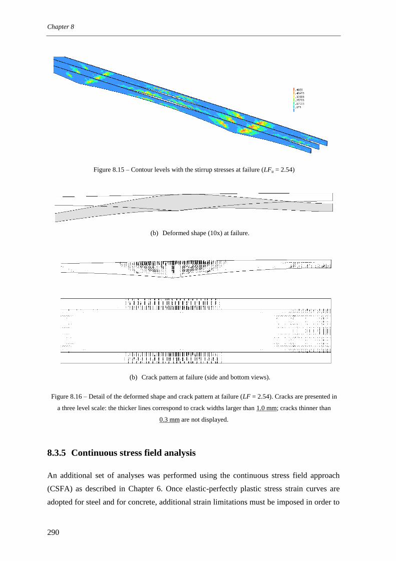
Chapter 8

290

Figure 8.15 – Contour levels with the stirrup stresses at failure (LFu = 2.54)

(b) Deformed shape (10x) at failure.

(b) Crack pattern at failure (side and bottom views).

Figure 8.16 – Detail of the deformed shape and crack pattern at failure (LF = 2.54). Cracks are presented in

a three level scale: the thicker lines correspond to crack widths larger than 1.0 mm; cracks thinner than

0.3 mm are not displayed.

8.3.5 Continuous stress field analysis

An additional set of analyses was performed using the continuous stress field approach

(CSFA) as described in Chapter 6. Once elastic-perfectly plastic stress strain curves are

adopted for steel and for concrete, additional strain limitations must be imposed in order to


291

avoid an overestimation of the structural capacity. This way, failure is assumed to occur

when the first of the following events takes place: the tensile strains in the reinforcing steel

exceed 15‰; the strains in the prestressing steel exceed 20‰; or the compressive concrete

strains exceed 4‰ (which is equivalent to having Emax ≤ 2). In cases where the ultimate

load is strongly dependent on these strain limits and the safety margin is low, a refined

calculation of the deformation capacity using the F-CMM is recommended.

Although the calculation of force-deformation curves is not the purpose of the CSFA, the

calculated curves for load combinations LC1 and LC3 are compared to those obtained with

the F-CMM, see Figure 8.17. The dashed portion of the curves corresponds to equilibrium

states beyond the theoretical failure load determined on the basis of the strain limitation

criteria. The events marked in the curves were defined in accordance to the strain limits

defined above.

0

1

2

3

0 0.5 1 1.5

Load

fac

tor

LF


F-CMM - Mean

CSFA - MeanLC1

LFu = 2.44:

tendon failure at section nº23

LF = 2.60: concrete

crushing in the bottom slab, near P1

LF = 2.97: web crushing in

the first span, near P1

LF = 2.9: stirrup

failure in the central web, near section nº23

0

1

2

3

0 0.2 0.4 0.6

Load

fac

tor

LF


F-CMM-Mean

CSFA-Mean LC3

LFu = 2.43:

concrete crushing in the bottom

slab, near P2

LF = 2.54: tendon

failure over P1

LF = 2.65: web crushing in

the third span, near P2

Figure 8.17 – Force-displacement curves.

The continuous stress field in the central web of the 3rd

span at impending failure is

depicted in Figure 8.18 for load combination LC3. Due to the contribution of the inclined

tendons, a slightly deviated stress field develops [80]. The average inclination of the

compressive stress field is such that cot’ varies between 1.35 and 1.40, which agrees

remarkably well with what has been considered in the member level assessment. If a large

ductility for the compressed concrete in the bottom slab is assumed, shear failure is

predicted to occur for LF = 2.65.

Chapter 8

292

Figure 8.18 – Continuous stress fields in the central web of the 3rd

span for load combination LC3.


In this chapter it was shown how to define a global resistance factor based on a semi-


variation of the input variables. A simple safety format that is compatible with NLFEA

assumptions was formulated, following closely what is being proposed by Cervenka [55]

and the new CEB-FIP Model Code 2010 [87]. Besides enabling the use of updated

information regarding the material properties, the proposed procedure allows performing

reliability differentiation based on risk analysis considerations and on the expected

remaining service life of the structure, being therefore suitable for the safety examination

of existing bridges.

A traditional safety assessment at the member level led to the conclusion that the bridge

fulfils the safety requirements without any safety margin. The bridge was predicted to be

critical in bending, namely in the hogging moment regions of the 3rd

span and in the region

of the 2nd

span where the bottom slab continuity tendons are anchored. The system level

assessment using the F-CMM revealed that the bridge has, in fact, an appreciable safety

margin, which can be explained by its redistribution capacity. Failure was predicted to

occur by concrete crushing in the hogging bending moment regions irrespective of the load

combination being considered. The results obtained for the load combinations LC1 and

LC2, in which the traffic load was positioned so as to maximize the bending moment in the

sections where the bottom continuity tendons are anchored, revealed that tendon and

stirrup failure were about to occur. If the safety margin had not turned out so comfortable,

the analysis should proceed to a sensitivity study varying the parameters defining the

ductility of the steel.

A set of analyses was also performed using the continuous stress field model developed in

Chapter 6. As elastic-perfectly plastic stress-strain relations are used, in statically

indeterminate structures additional strain limits are required in order to avoid

overestimations of the load carrying capacity. This way notional failure loads were


293

obtained for each load combination. These compared favourably with the more accurate

estimates using the F-CMM, which is an indicator of the adequacy of the adopted strain

limits.

Since the bridge safety is not at risk, the installation of a surveillance system, constituted

by a set of sensors monitoring the activity of some selected cracks, and remotely

transmitting the information for periodic or continuous assessment, could provide valuable

information to the bridge owner, enabling increasing the period between periodic visual

inspections while the planned intervention is scheduled. This intervention is justified by

the concerns related to the durability of the bridge.

295

9 Summary and conclusions

This thesis was oriented towards the development of a harmonised set of models enabling a

stepwise approach to the safety assessment of existing concrete bridges. Nonlinear finite

element analysis (NLFEA) was adopted as the reference tool for the accurate assessment of

the load-carrying capacity. Since many structural elements can be idealized as an assembly

of membrane elements, special attention was paid to the analysis of RC panels subjected

mainly to in-plane shear and axial forces. Based on the detailed models developed for

NLFEA, simplified formulations were derived for shear strength assessment of structural

elements containing at least the minimal amount of shear reinforcement and a case study

was presented aimed at illustrating the applicability of the developed tools. In the

following, a brief summary of the work developed in each chapter is presented.

Chapter 2

In Chapter 2, the main features of concrete behaviour when subjected to short term loading

conditions were examined. Four basic phenomena were identified at the macro-level

governing the behaviour of structural concrete elements: tensile fracture; bond shear stress

transfer between the reinforcements and the surrounding concrete; shear stress transfer

trough rough cracks; and compressive behaviour under uniaxial or multiaxial stress

conditions. The experimental procedures, and corresponding theoretical models, aimed at

providing a description of each of the above mentioned phenomena were discussed in

some detail. The concepts and terminology introduced in this chapter were thoroughly used

throughout the thesis.

Chapter 3

In Chapter 3, a new model considering fixed and interlocked cracks, the F-CMM, was

proposed for the analysis of RC panels subjected to in-plane shear and axial stresses. The

model complements the Cracked Membrane Model of Kaufmann and Marti (here

designated as R-CMM) by extending its concept to the case of fixed and interlocked cracks

capable of transferring shear and normal stresses. This enabled a more consistent

reproduction of shear sliding failures in orthotropically reinforced panels, a better fit to the

observed deformational behaviour and improved calculations of the shear strength.

Chapter 9

296

Equilibrium is formulated in terms of stresses at the cracks and compatibility is formulated

in terms of average strains. The consideration of the local mechanical effects that take

place at the cracks, - such as aggregate interlock, crack bridging and softened compressed

concrete behaviour - , together with the bond stress transfer mechanics described according

to the Tension Chord Model (TCM), allowed a rational derivation of both local and

average stress/strain fields and a deeper understanding of the complex mechanics

governing the behaviour of cracked RC membranes. Nevertheless, the model was kept

sufficiently simple for implementation in a robust finite element formulation for structural

analysis. A validation campaign was carried out using a database with the experimental

results of 54 RC panels tested under in-plane shear and axial stress conditions. Good

agreement was found between the predicted and the observed shear strengths, failure

modes and deformational behaviour. The database covered a wide range of reinforcement

ratios and concrete strengths ensuring that the model is generally applicable.

Chapter 4

In Chapter 4, the basic concepts behind the computational models for nonlinear analysis of

structural concrete elements were presented and a total strain constitutive model for

accommodating the RC cracked membrane element constitutive laws devised in Chapter 3

was developed. The model comprises a set of state variables that continuously monitor

damage evolution in concrete and enable the establishment of suitable loading/unloading

conditions. Strain localization issues were dealt with using a description of the

displacement field based on the ―weak discontinuities‖ concept, which was still found to

present the best compromise between accuracy, simplicity and economy of computer

resources. Uncracked concrete nonlinear behaviour in biaxial compression was formulated

in a very efficient way using the concepts of equivalent stress and equivalent strain. Due to

the adoption of a dedicated phenomenological model for shear stress-transfer between

rough cracks, which includes both shear and dilatancy stresses, special attention was paid

to the equilibrium and compatibility conditions in cases of two orthogonal cracks arising in

the same integration point. The model for reinforcing steel was formulated according to the

Tension Chord Model and clear physical assumptions were used for establishing the

loading/unloading conditions and the behaviour under reversed loading paths. The

implemented algorithms were described in detail and some simple validation examples

were presented for illustrating the model response. The implementation was extended to

shell elements and good agreement was obtained when comparing the calculated results

Summary and conclusions

297

with experimental data. Good convergence characteristics were exhibited in the analysed

examples.

Chapter 5

In Chapter 5, a validation campaign was undertaken using a set of experimental tests on

large scale shear critical structural elements. Both continuity and discontinuity regions

were analysed. The model proved capable of reproducing shear failures in demanding

situations, such as the ones involving plastic strains in the longitudinal reinforcement.

Good estimates of the failure modes, failure loads, cracking patterns and crack widths were

achieved. The implementation proved robust and the force-deformation responses could be

computed in the post-peak range, thus allowing the identification of the failure

mechanisms. Although the focus was driven to modelling of shear failures in shear

reinforced concrete girders, an example was presented of a concrete girder failing in

bending. In this case, good estimates of the deformation capacity in the post-yield stage

and an accurate sizing of the plastic hinge regions were obtained. In spite of the overall

good results, some limitations were found. (1) Although not severe, the deformation

capacity of the stirrups is somewhat underestimated whenever failure is governed by

stirrup rupture. This is attributed to the fact that the model cannot reproduce bond slip

occurring across several cracks; (2) Despite the fact that the F-CMM can reproduce the

associated crack kinematics, the shear sliding failure mode could not always be clearly

evidenced due to anticipated crushing of web concrete. In fact, localization of the shear

displacements along a well defined crack could not be obtained in cases where the

compressive stresses in the web were high and plastic strains in the tensile reinforcement

were observed (specimens MVN2 and MVN3). This seems to indicate that the adopted

softening law, which is based on the results obtained on RC panels, gives conservative

estimates of the effective compressive strength in discontinuity regions similar to those of

specimens MVN2 and MVN3. Nonetheless, the failure loads and the force-deformations

curves were still in good agreement with the observed ones and the failure region is

correctly identified; (3) Finally, due to the kinematic description of the displacement field

based on the concept of weak discontinuities the web crushing failure is systematically

localized along a row of finite elements, instead of spreading throughout the whole web.

Although this effect has almost no implications in the calculation of the peak load, it

influences the computation of the load carrying mechanisms in the post-peak regime.

Chapter 9

298

Chapter 6

In Chapter 6 simplified models for engineering practice were presented. Given the fact that

flexural strength can be considered to be satisfactorily predicted in current design methods,

the focus of these simplified formulations was driven to shear dominated problems. In

Chapter 3 it was shown that the R-CMM can be obtained from the F-CMM by imposing an

additional constraint related with the coincidence of the principal axes of concrete stress at

the cracks and average strain. The equilibrium equations and the constitutive laws are

simplified at the cost of some decrease in accuracy. The R-CMM can be further simplified

by neglecting the concrete tensile strength and the bond stress transfer effects, resulting in

a limit analysis formulation following more closely the assumptions usually adopted in

engineering practice. It is simpler to use and, in the case of RC panels, comes down to a set

of closed form expressions for the yield conditions. However, in the case of a structural

analysis, the relevant outcomes are simply the stress fields expressing the equilibrium at

failure conditions and the corresponding ultimate load. This tool can be extremely useful

whenever the choice of an appropriate discontinuous stress field is not trivial and

establishes the link between limit analysis methods and the numerical models developed in

the previous chapters. For the case of continuity regions, a simple sectional analysis

method was derived directly from the yield conditions considering a constant shear stress

distribution along the cross-section height. The resulting expressions are formally similar

to those of the variable angle truss model adopted in the recent European codes. However,

by allowing the exploitation of a wider range of values for the inclination of the struts and

the incorporation of the effect of the longitudinal reinforcement/prestressing steel strains in

the definition of fc,ef, the proposed method is suitable for an intermediate shear strength

assessment of an existing concrete bridge.

Chapter 7

In Chapter 7 a 30 year-old post-tensioned concrete box-girder bridge exhibiting consistent

cracking patterns throughout the deck was examined in detail. Cracks were observed in the

webs, mainly at the joints of segmental construction, and in the bottom slab. Besides a

detailed visual inspection and some material characterization studies, a preliminary non-

destructive inspection using gamma-rays was undertaken in order to evaluate the feasibility

of an exhaustive inspection campaign using this technology. This was motivated by the

uncertainty regarding the condition of post-tension tendons. The obtained gammagraphies


299

revealed no grouting defects or corrosion signs in the wires. This study should now be

completed in order to collect more data in different locations of the deck.

The bridge was also monitored during a controlled load test and along 4 days under normal



loads and daily thermal variations. Crack opening variations of 0.13mm were measured

with four loaded trucks on the deck producing a live-load bending moment approximately

65% of that produced by the load model of the Portuguese code used in the original design

and still in force today. Due to the daily thermal variations in a 4 days measuring period,

the crack width variations reached 0.1mm. In spite of the measured crack activity, the

bridge exhibited linear elastic behaviour during the load test. Although the measured

response in some sensors was systematically more flexible than that calculated, the

response to vehicle loading compared reasonably well with that calculated considering the

uncracked stiffness of the deck. Since no baseline condition is available, no definite

conclusions could be drawn from this set of results. In fact, stiffness changes due to

localized cracks are expected to be small and difficult to evaluate without a direct and

careful comparison with previous measurements - it must be noted that only the cracks that

are continuous between the bottom slab and the webs effectively decrease the bending

stiffness. Still, the obtained results can serve as a comparison basis for future tests and

show that the structural condition of the bridge does not require immediate intervention.

In order to explain the origin of the observed cracking patterns, the bridge was analysed

with both 2D and 3D finite element models taking into account the construction sequence

and the time-dependent evolution of the sectional forces due to the effects of creep,

shrinkage and prestress steel relaxation. The obtained results indicate that the observed

cracking patterns are not linked to prestress steel corrosion and are mainly due to an

inadequate layout of the prestress tendons together with the adoption of a very low

ordinary reinforcement ratio in the longitudinal direction. In this respect, the 3D analysis

proved essential to confirm that the decompression limit state both in the bottom slab and

in the webs is almost reached in the long-term considering only the action of permanent

loads. The analysis of the local stress conditions around the tendon anchorages was crucial

in order to understand the origin of the observed cracking patterns. In these circumstances,

average residual crack widths larger than 0.3 mm are to be expected, which agrees well

with the mapped crack widths.

Chapter 9

300

Chapter 8

In Chapter 8 it was shown how to define a global resistance factor based on a semi-


variation of the input variables. A simple safety format that is compatible with NLFEA

assumptions was formulated, following closely what is being proposed by Cervenka [55]

and in the new CEB-FIP Model Code 2010 [87]. Besides enabling the use of updated

information regarding the material properties, the proposed procedure allows performing

reliability differentiation based on risk analysis considerations and on the expected

remaining service life of the structure, being therefore suitable for the safety examination

of existing bridges.

A traditional safety assessment at the member level led to the conclusion that the bridge

fulfils the safety requirements without any safety margin. The bridge was predicted to be

critical in bending, namely in the hogging moment regions of the 3rd

span and in the region

of the 2nd

span where the bottom slab continuity tendons are anchored. The system level

assessment using the F-CMM revealed that the bridge has, in fact, an appreciable safety

margin, which can be explained by its redistribution capacity. Failure was predicted to

occur by concrete crushing in the hogging bending moment regions irrespective of the load

combination being considered. The results obtained for the load combinations in which the

traffic load was positioned so as to maximize the bending moment in the sections where

the bottom continuity tendons are anchored revealed that tendon and stirrup failure were

about to occur. If the safety margin had not turned out so comfortable, the analysis should

proceed to a sensitivity study varying the parameters defining the ductility of the steel.

A set of analyses was also performed using the continuous stress field model developed in

Chapter 6. As elastic-perfectly plastic stress-strain relations are used, in statically

indeterminate structures additional strain limits are required in order to avoid

overestimations of the load carrying capacity. In this way notional failure loads were

obtained for each load combination. These compared favourably with the more accurate

estimates using the F-CMM, which is an indicator of the adequacy of the adopted strain

limits.


301

9.1 Recommendations for future research

RC cracked membrane element

As shown by Alvarez [3], refined calculations of the steel stresses at the cracks in the post-

yielding stage can be made if more realistic stress-strain laws are adopted for the rebars

instead of the simplified bi-linear law adopted in this work. This requires the generalization

of the TCM expressions (3.38) and (3.39) and may improve the estimates of the

deformation capacity whenever the reinforcement ratio is low. The influence of the

reinforcement ductility class on the failure modes and failure loads of both RC panels and

structural concrete elements should be investigated.

The crack shear stress transfer model must be generalized for high strength concrete. Also

a dowel action model can be included in the formulation, thereby allowing the examination

of the dowel action effects on the shear strength and on the reduction of the apparent

yielding stress of the reinforcement. The RC cracked membrane element formulation

presented in Chapter 3 could be also extended to accommodate non-orthogonal

reinforcement meshes.

Following the works of Vecchio [241], Bentz [24] and Mohr et al [161], both the F-CMM

and the R-CMM can be implemented in a layered beam finite element formulation. This

would enable a more efficient study of the shear response in beam continuity regions and

would allow tracing accurate (N, M, V) interaction diagrams for different types of cross-

sections. Moreover, this type of elements is widely used in commercial finite element

codes dedicated to bridge analysis and design and would enhance the applicability of the

developed models in engineering practice.

NLFEA model based on the RC cracked membrane element

The use of a non-local formulation for improving mesh objectivity with regard to

compression failures should be attempted. This could enhance the predictions of the

deformation capacity of plastic hinge regions as well as a more accurate reproduction of

web crushing or web sliding failures.

It is also advised to extend the validation campaign. Similarly to what has been performed

with RC cracked membrane element, the database of analysed shear reinforced girders

should be increased in order to cover a broader range of reinforcement and prestressing

ratios. Moreover, other structural elements should be included, the most typical being shear

walls, deep beams and elements subjected to torsion. Much is learned during these

Chapter 9

302

validation analyses, eventually leading to the improvement of some features of the model.

This would also be important to establish the model uncertainty parameter to be adopted in

the safety format described in Chapter 8.

The interaction between out-of-plane bending and in-plane shear should also be evaluated

and compared to experimental evidence. As evidenced in Chapter 8, this interaction occurs

in the webs of box-girder bridges and may govern the shear capacity.

The application of the developed NLFEA model in serviceability calculations requires the

generalization of the formulation so that residual crack openings can be determined with

good accuracy. Although previous overloading may cause crack development, it is the

residual crack opening at a pre-determined operating load level that should be compared to

the target value. Therefore, reversed bond action and re-contact stress at crack closing

should be introduced in the model. Moreover, concrete time dependent effects, such as

shrinkage and creep, should be also included. This is an important feature for realistic

serviceability analyses of segmental bridges, such as the one analysed in Chapter 7.


The model for continuous stress field analysis of structural elements developed in Chapter

6 revealed great potential both for academic and practical engineering purposes. Since

simple constitutive laws are used, the model can be used as an introductory tool in courses

concerned to NLFEA. Moreover, it can serve as an auxiliary tool in advanced structural

concrete courses treating discontinuous stress fields/strut-and-tie models. In engineering

practice, this model can be used in the analysis, design and assessment of discontinuity

regions with complex geometry by structural engineers with no relevant expertise in

NLFEA. However, and as remarked in Chapter 8, due to the adoption of elastic-perfectly

plastic stress-strain laws, additional strain limits must be imposed in order to avoid

overestimation of the load carrying capacity of statically indeterminate structures.

Although tentative values have been adopted in the analysis of the N.S da Guia Bridge,

these limits should be confirmed after comparison with experimental evidence and/or

numerical analyses with the F-CMM.

As for the simplified analytical model for continuity regions, its extension to problems

involving torsion should be made. The applicability of this model in the analysis of the

interaction between out-of-plane bending and in-plane shear should be evaluated.


303

Safety formats for NLFEA

The safety format for NLFEA described in Chapter 8 should be thoroughly evaluated

trough comparison with the results obtained with higher order reliability or simulation

methods. A clear set of recommendations could then be issued in future codes of practice,

which would certainly contribute to increasing use of more advanced analysis tools in the

safety examination of existing concrete bridges.

305

References

[1] AASHTO. (2004). AASHTO LFRD Bridge Design Specifications, Washington D. C.

[2] Alfaiate, J. M. V. (1992). "Estudo e Modelação do Comportamento do Betão Fissurado," Tese de

Doutoramento, Instituto Superior Técnico, Lisboa.

[3] Alvarez, M. (1998). "Einfluss des Verdunverhaltens auf das Vermormungsvermögen von Stahlbeton,"

Doctoral Thesis, Swiss Federal Institute of Technology Zurich, Zurich.

[4] Angst, U., Elsener, B., Larsen, C. K., and Vennesland, O. (2009). "Critical chloride content in reinforced

concrete — A review " Cement and Concrete Research, 39(12), 1122-1138.

[5] Aspiotis, J. (1993). "Compression Softening of High Strength Reinforced Concrete Elements," Master

Thesis, University of Toronto, Toronto.

[6] Barlett, F. M., and MacGregor, J. G. (1996). "Statistical Analysis of the Compressive Strength of

Concrete in Structures." ACI Materials Journal, 93(2), 158-168.

[7] Barlett, F. M., and MacGregor, J. G. (1999). "Variation of In-Place Concrete Strength in Structures." ACI

Materials Journal, 96(2), 261-271.

[8] Barras, P., Matteis, D., Derais, J.-F., Duviard, M., Guillot, D., Lacombe, J.-M., Ojeda, V., Paillusseau, P.,

and Reinhardt, J.-M. (2003). Design guide - Prestressed concrete bridges built using the cantilever

method, Sétra.

[9] Bazant, Z. P. (1986). "Mechanics of distributed cracking." Appl Mech Rev, ASME, 39(5), 675-705.

[10] Bazant, Z. P. (1991). "Why Continuum Damage is Nonlocal: Micromechanics Arguments." Journal of

Engineering Mechanics, 117(5), 1070-1087.

[11] Bazant, Z. P., and Baweja, S. (1995). "Creep and shrinkage prediction model for analysis and design of

concrete structures - model B3." Materials and Structures, 28(6), 357-365.

[12] Bazant, Z. P., and Gambarova, P. G. (1980). "Rough crack models in reinforced concrete." Journal of

Structural Engineering, 106(4), 819-842.

[13] Bazant, Z. P., and Gambarova, P. G. (1984). "Crack Shear in Concrete: Crack Band Microplane Model."

Journal of Structural Engineering, 110(9), 2015-2035.

[14] Bazant, Z. P., and Jirasek, M. (2002). "Nonlocal Integral Formulations of Plasticity and Damage: Survey

of Progress." Journal of Engineering Mechanics, 128(11), 1119-1149.

[15] Bazant, Z. P., Li, G.-H., Yu, Q., Klein, G., and Kristek, V. (2009). "Explanation of Excessive Long-

Time Deflections of Collapsed Record-Span Box Girder Bridge in Palau - Preliminary Structural

Engineering Report No. 08-09/A222e." Infrastructure Technology Institute, McCormick School of

Engineering and Applied Science, Northwestern University, Evanston, Illinois.

[16] Bazant, Z. P., and Lin, F. B. (1989). "Nonlocal Smeared Cracking Model for Concrete Fracture."


[17] Bazant, Z. P., and Oh, B. H. (1983). "Crack band theory for fracture of concrete." Materials and

Stuctures, 16(1), 155-177.

[18] Bazant, Z. P., and Yu, Q. (2005). "Designing Against Size Effect on Shear Strength of reinforced

Concrete Beams Without Stirrups: 2. Verification and Calibration." Journal of Structural

Engineering, 131(12), 1886-1896.

[19] Bazant, Z. P., and Yu, Q. (2010). "Modelling of concrete creep and hygrothermal deformations, and

computation of their structural effects." Computational Modelling of Concrete Structures: EURO-C

2010, Rohrmoos/Schladming.

Chapter 10

306

[20] Belarbi, A. (1991). "Stress-Strain Relationships of Reinforced Concrete in Biaxial Tension-

Compression," Doctoral Thesis, University of Houston, Houston.

[21] Belarbi, A., and Hsu, T. T. C. (1994). "Constitutive Laws of Concrete in Tension and Reinforcing Bars

Stiffened by Concrete." ACI Structural Journal, 91(4), 465-474.

[22] Belarbi, A., and Hsu, T. T. C. (1995). "Constitutive Laws of Softened Concrete in Biaxial Tension-

Compression." ACI Structural Journal, 92(5), 562-573.

[23] Belleti, B., Cerioni, R., and Ivori, I. (2001). "Physical Approach for Reinforced-Concrete (PARC)

Membrane Elements." Journal of Structural Engineering, 127(12), 1412-1426.

[24] Bentz, E. C. (2000). "Sectional Analysis of Reinforced Concrete Members," Doctoral Thesis, University

of Toronto, Toronto.

[25] Bentz, E. C. (2005). "Explaining the Riddle of Tension Stiffening Models for Shear Panel Experiments."


[26] Bentz, E. C., and Collins, M. P. (2006). "Development of the 2004 Canadian Standards Association

(CSA) A23.3 shear provisions for reinforced concrete." Canadian Journal of Civil Engineering, 33,

521-534.

[27] Bhide, S. B., and Collins, M. P. (1989). "Influence of Axial Tension on the Shear Capacity of

Reinforced Concrete Members." ACI Structural Journal, 86(5), 570-581.

[28] Bloem, D. L. (1968). "Concrete Strength in Structures." ACI Journal, 65(3), 176-187.

[29] Borst, R. (1986). "Nonlinear Analysis of Frictional Materials," Doctoral Thesis, Technical University of

Deflt, Delft.

[30] Borst, R. (1987). "Smeared cracking, plasticity, creep and thermal loading - A unified approach."

Computer Methods in Applied Mechanics and Engineering, 62(1), 89-110.

[31] Borst, R. (1993). "A generalization of J2-flow theroy for polar continua." Computer Methods in Applied

Mechanics and Engineering, 103, 347-362.

[32] Borst, R., and Boogaard, A. H. (1994). "Finite-Element Modeling of Deformation and Cracking in

Early-Age Concrete." Journal of Engineering Mechanics, 120(12), 2519-2534.

[33] Borst, R., and Mühlhaus, H.-B. (1992). "Gradient-dependent plasticity: Formulation and algorithmic

aspects." International Journal for Numerical Methods in Engineering, 35, 521-539.

[34] Borst, R., and Nauta, P. (1985). "Non-orthogonal cracks in a smeared finite element model."

Engineering Computations, 2, 35-46.

[35] Borst, R., Sluys, L. J., Mühlhaus, H.-B., and Pamin, J. (1993). "Fundamental issues in finite element

analyses of localization of deformation." Engineering Computations, 10, 99-121.

[36] BRIME. (2001). "Deliverable D14 - Final Report." Available from:

http://www.trl.co.uk/brime/deliver.htm.

[37] Bujadham, B., and Maekawa, K. (1992). "The Universal Model for Stress Transfer Across Cracks in

Concrete." Proc. of the JSCE, 17, 277-287.

[38] Campbell, R. H., and Tobin, R. E. (1967). "Core and Cylinder Strengths of Natural and Lightweight

Concrete." ACI Journal, 64(4), 190-195.

[39] Carino, N. J., and Malhotra., V. M. (2004). "Handbook on Non-destructive Testing of Concrete." CRC

Press, Boca Raton.

[40] CEB. (1993). CEB-FIP Model Code 1990, Thomas Telford, London.

[41] CEB. (1996). "RC elements under cyclic loading. State-of-the-art report.", Thomas Telford, London.

[42] CEN. (2002). EN 1990 - Eurocode: Basis of structural design, European Comitee for Standardization,

Brussels.

[43] CEN. (2003). EN 1991-2 Eurocode 1: Actions on structures - Part 2: Traffic loads on bridges, European

Comitee for Standardization, Brussels.

http://www.trl.co.uk/brime/deliver.htm

References

307

[44] CEN. (2003). NP EN 12504-1:2003 Ensaios do betão nas estruturas - parte 1: Carotes. Extracção,

exame e ensaio à compressão, IPQ.

[45] CEN. (2003). NP EN 12504-2:2003 Ensaios do betão nas estruturas - parte 2: Ensaio não destrutivo.

Determinação do índice esclerométrico., IPQ.

[46] CEN. (2004). Eurocode 2: Design of concrete structures - Part 1-1: General rules and rules for

buildings, European Comitee for Standardization, Brussels.

[47] CEN. (2007). NP EN 12504-2:2007 Ensaios do betão nas estruturas - parte 3: Determinação da força

de arranque, IPQ.

[48] CEN. (2007). NP EN 12504-2:2007 Ensaios do betão nas estruturas - parte 4: Determinação da

velocidade de propagação dos ultra-sons, IPQ.

[49] CEN. (2008). NP EN 13791 - Avaliação da resistência á compressão do betão nas estruturas e em

produtos pré-fabricados, IPQ.

[50] CEN. (2009). NP EN 1991-5:2009. Eurocódigo 1 - Acções em estruturas. Parte 1-5: Acções gerais.

Acções térmicas. , IPQ.

[51] CEN TC 250/SC2. (2008). Eurocode 2 Commentary, European Concrete Platform, Brussels.

[52] Cerioni, R., Iori, I., Michelini, E., and Bernadi, P. (2008). "Multi-directional modeling of crack pattern

in 2D R/C members." Engineering Fracture Mechanics, 75, 615-628.

[53] Cerruti, L. M., and Marti, P. (1987). "Staggered shear design of concrete beams: large-scale tests."

Canadian Journal of Civil Engineering, 14, 257-268.

[54] Cervenka, J., and Cervenka, V. (2010). "On the uniqueness of numerical solutions of shear failure of

deep concrete beams: Comparison of smeared and discrete crack approaches." EURO-C 2010:

Computational modelling of concrete structures, 281-290.

[55] Cervenka, V. (2008). "Global Safety Factor for Nonlinear Calculation of Reinforced Concrete." Beton-

und Stahlbetonbau, 103, 37-42.

[56] Cervenka, V., and Cervenka, J. (1996). "Computer simulation as a design tool for concrete structures."

ICCE-96 - Second International Conference in Civil Engineering on Computer Applications,

Research and Practice, Bahrain.

[57] Cervenka, V., Pukl, R., Ozbolt, J., and Eligehausen, R. (1995). "Mesh sensitivity effects in smeared

finirte element analysis of concrete fracture." Fracture Mechanics of Concrete structures

(FRAMCOS II), Zurich, 1387-1396.

[58] Chen, W. F. (1982). Plasticity in Reinforced Concrete, McGraw-Hill.

[59] Chintrakarn, R. (2001). "Minimum Shear Steel and Failure Modes Diagram of Reinforced Concrete

Membrane Elements," Master Thesis, University of Houston, Houston.

[60] Collins, M. P. (1978). "Towards a Rational Theory for RC Members in Shear." Journal of the Structural

Division ASCE, 104(4), 649-666.

[61] Collins, M. P. (1998). "Procedures for Calculating the Shear Response of Reinforced Concrete Elements:

A Discussion." Journal of Structural Engineering, 124(12), 1485-1488.

[62] Collins, M. P., and Kuchma, D. (1999). "How Safe Are Our Large, Lightly Reinforced Concrete Beams,

Slabs, and Footings?" ACI Structural Journal, 96(4), 482-490.

[63] Collins, M. P., Mitchell, D., Adebar, P., and Vecchio, F. J. (1996). "A General Shear Design Method."

ACI Structural Journal, 93(1), 36-45.

[64] Cornelissen, H. A. W., Hordijk, D. A., and Reinhardt, H. W. (1986). "Experimental determination of

crack softening characteristics of normal weight and lightweight concrete." Heron, 31(2).

[65] COST-345. (2004). "Procedures Required for Assessing Highway Structures - Joint report of Working

Groups 2 and 3: methods used in European States to inspect and assess the condition of highway

structures." European Commission - Directorate General Transport and Energy. Available from:

http://cost345.zag.si/final_reports.htm.

http://cost345.zag.si/final_reports.htm

Chapter 10

308

[66] COST-345. (2004). "Procedures Required for the Assessment of Highway Structures - Final report."

European Commission - Directorate General Transport and Energy. Available from:

http://cost345.zag.si/final_reports.htm.

[67] Costeira Silva, P. (2008). "Comportamento de Estruturas de Betão Reforçadas por Colagem Exterior de

Sistemas CFRP," Doctoral Thesis, Faculty of Engineering of the University of Porto, Porto.

[68] Costeira Silva, P., Juvandes, L., and Figueiras, J. A. (2005). "Inspecção Visual das Paredes do Caixão do

Tabuleiro da Ponte de N. S. da Guia - Relatório Interno." LABEST, Universidade do Porto,

Faculdade de Engenharia, Porto.

[69] Crisfield, M. A. (1981). "A fast incremental/iterative solution procedure that handles snap-through."

Computer & Structures, 13, 55-62.

[70] Crisfield, M. A. (1991). Non-linear Finite Element Analysis of Solids and Structures, vol. 1: Essentials.,

John Wiley & Sons, Chichester.

[71] Crisfield, M. A., and Wills, J. (1989). "Analysis of R/C Panels Using Different Concrete Models."

Journal of Engineering Mechanics, 115(3), 578-597.

[72] CSA. (2004). Design of Concrete Structures, CSA A23.3-04, Canadian Standards Association.

[73] Dérobert, X., Aubagnac, C., and Abraham, O. (2002). "Comparison of NDT techniques on a post-

tensioned beam before its autopsy." NDT&E international, 35, 541-548.

[74] Dias da Silva, V. (1995). Mecânica e Resistência dos Materiais, EDILIBER Editora, Coimbra.

[75] Elices, M., and Planas, J. (1989). "Material Models." Fracture Mechanics of Concrete Structures. Report

of the RILEM Comitee 90-FMA, L. Elfgren, ed., Chapman and Hall, London, 16-66.

[76] Feenstra, P. H. (1993). "Computational Aspects of Biaxial Stress in Plain and Reinforced Concrete,"

Doctoral Thesis, Delft University of Technology, Delft.

[77] Feenstra, P. H., Borst, R., and Rots, J. G. (1991). "Numerical Study on Crack Dilatancy. II:

Applications." Journal of Engineering Mechanics, 117(4), 754-769.

[78] Félix, C. (2004). "Monitorização e análise do comportamento de obras de arte," Doctoral Thesis,

Faculdade de Engenharia da Universidade do Porto, Porto.

[79] Fernández-Ruiz, M., and Muttoni, A. (2007). "On Development of Suitable Stress Fields for Structural

Concrete." ACI Structural Journal, 104(4), 495-502.

[80] Fernández-Ruiz, M., and Muttoni, A. (2008). "Shear Strength of Thin-Webbed Post-Tensioned Beams."


[81] Fernández-Ruiz, M., and Muttoni, A. (2009). "Applications of Critical Shear Crack Theory to Punching

of Reinforced Concrete Slabs with Transverse Reinforcement." ACI Structural Journal, 106(4),

485-494.

[82] Fernández-Ruiz, M., Rodrigues, R. V., and Muttoni, A. (2009). "Dimensionnement et vérification des

dalles de roulement des ponts routiers." Ecole Polytechnique Fédérale de Lausanne (EPFL),

Laboratoire de Construction en Béton (IS-BETON), Office fédéral des routes (OFROU), Lausanne.

[83] Ferraz, M. (2010). "Modelo para avaliação do comportamento estrutural de obras de arte," Doctoral

Thesis, Faculdade de Engenharia da Universidade do Porto, Porto.

[84] fib. (1999). "Bulletin nº1: Structural Concrete. Text book on Behaviour, Design and Performance.

Vol.1." fib, Lausanne.

[85] fib. (2000). "Fib bulletin 10: Bond of reinforcement in concrete - State-of-art report." fib, Lausanne.

[86] fib. (2008). "A Practitioner's Guide to Computer-Based Modelling of Structural Concrete (bulletin 45)."

fib, Lausanne.

[87] fib. (2010). Model Code 2010 - First complete draft, fib, Lausanne.

[88] Figueiras, J., Juvandes, L., and Oliveira, L. (1999). "Reforço Experimental da Laje do Tabuleiro da

Ponte de N. S. da Guia em Ponte de Lima - Relatório Técnico." LABEST, Universidade do Porto,

Faculdade de Engenharia, Porto.

http://cost345.zag.si/final_reports.htm

References

309

[89] Figueiras, J. A. (1983). "Ultimate Load Analysis of Anisotropic and reinforced Concrete Plates and

Shells," Doctoral Thesis, University College of Swansea, Swansea, Walles.

[90] Frigerio, T., Mariscotti, M. A. J., Ruffolo, M., and Thieberger, P. (2004). "Development and application

of computed tomography in the inspection of reinforced concrete." Insight, 46(12).

[91] Gaspar, R., and Stucchi, F. R. (2009). "Dimensionamento das almas de pontes celulares." Revista

Portuguesa de Engenharia de Estruturas, Série II(6), 41-46.

[92] Gonçalves, A. F. (1987). "Resistência do betão nas estruturas," Doctoral Thesis, Laboratório Nacional

de Engenharia Civil, Lisboa.

[93] Hadamard, J. (1902). "Sur les problèmes aux dérivées partielles et leur signification physique."

Princeton University Bulletin, 49-52. .

[94] Hawkins, N. M., and Kuchma, D. A. (2007). "NCHRP Report 579 - Application of LFRD Bridge design

Specifications to High-Strength Structural Concrete: Shear Provisions." Transportation Research

Board, Washinton, D.C.

[95] Hawkins, N. M., and Kuchma, D. A. (2007). "NCHRP Report 579 - Application of LFRD Bridge design

Specifications to High-Strength Structural Concrete: Shear Provisions (Appendices)."

Transportation Research Board, Washington, D.C.

[96] Henriques, A. A. (1998). "Aplicação de Novos Conceitos de Segurança no Dimensionamento do Betão

Estrutural," Doctoral Thesis, Faculdade de Engenharia da Universidade do Porto, Porto.

[97] Hernandez, H. D., and Gamble, W. L. (1975). "Time-dependent losses in prestressed concrete

construction." University of Illinois.

[98] Higgins, C., Miller, T. H., Rosowsky, D. V., Solomon, C. Y., Potistouk, T., Daniels, T. K., Nicholas, B.

S., Robelo, M. J., Lee, A.-Y., and Forrest, R. W. (2004). "Assessment methodology for diagonally

cracked reinforced concrete deck girders - Final Report SPR 350, SR 500-091." Oregon Department

of Transportation (ODOT) and Federal Highway Administration (FHWA).

[99] Hillerborg, A., Modéer, M., and Petersson, P. E. (1976). "Analysis of crack formation and crack growth

in concrete by means of fracture mechanincs and finite elements." Cement and Concrete Research,

6, 773-782.

[100] Hoang, L. C., and Nielsen, M. P. (1998). "Plasticity Approach to Shear Design." Cement and Concrete

Composites, 20, 437-453.

[101] Hordijk, D. A. (1992). "Tensile and tensile fatigue behaviour of concrete: experiments, modelling and

analyses." Heron, 37(1), 1-79.

[102] Hordijk, D. A., Van Mier, J. G. M., and Reinhardt, H. W. (1989). "Material Properties." Fracture

Mechanics of Concrete Structures. Report of the RILEM Comitee 90-FMA, L. Elfgren, ed.,

Chapman and Hall, London, 67-127.

[103] Hsieh, S.-S. (1981). "Elastic-plastic-fracture analysis of concrete structures," Doctoral Thesis, Purdue

University.

[104] Hsu, T. T. C., and Zhang, L. (1996). "Tension Stiffening in Reinforced Concrete Membrane Elements."


[105] Hsu, T. T. C., and Zhang, L. X. (1997). "Nonlinear Analysis of Membrane Elements by Fixed-Angle

Softened-Truss model." ACI Structural Journal, 94(5), 483-492.

[106] Hsu, T. T. C., and Zhu, R. R. H. (2002). "Softened Membrane Model for Reinforced Concrete

Elements in Shear." ACI Structural Journal, 99(4), 460-469.

[107] Ingraffea, A., and Saouma, V. (1985). "Numerical modelling of discrete crack propagation in

reinforced and plain concrete." Engineering Application of Fracture Mechanics, G. C. Sih and A. D.

Tommaso, eds., Martinus Nijhoff Publishers, Dordrecht, The Netherlands.

[108] Jansen, D. C., and Shah, S. P. (1997). "Effect of Length on Compressive Strain Softening of Concrete."


Chapter 10

310

[109] JCSS. (2001). "Probabilistic Assessment of Existing Structures - JCSS Report." D. Diamantidis, ed.,

RILEM Publications SARL

[110] Jirasek, M. (1998). "Nonlocal Models for Damage and Fracture: Comparison of Approaches."

International Journal of Solids and Structures, 35(31), 4133-4145.

[111] Jirasek, M. (2000). "Comparative study on finite elements with embedded discontinuities " Computer

Methods in Applied Mechanics and Engineering(188), 307-330.

[112] Jirasek, M. (2002). "Plasticity, Damage and Fracture." Technical University of Catalonia (UPC),

Barcelona.

[113] Jirasek, M., and Horák, M. (2010). "Localization properties of damage models." EURO-C 2010:


[114] Jirasek, M., Rolshoven, S., and Grassl, P. (2004). "Size effect on fracture energy induced by non-

locality " International Journal for Numerical and Analytical Methods in Geomechanics, 28(7-8),

653-670.

[115] Jirasek, M., and Zimmerman, T. (1998). "Analysis of Rotating Crack Model." Journal of Engineering

Mechanics, 124(8), 842-851.

[116] Kang, H. D., and Willam, K. (1999). "Localization Characteristics of Triaxial Concrete Model."


[117] Kaufmann, W. (1998). "Strength and Deformations of Structural Concrete Subjected to In-Plane Shear

and Normal Forces," Doctoral Thesis, Swiss Federal Institute of Technology Zurich, Zurich.

[118] Kaufmann, W. (2002). "Analysis and design of structural concrete elements subjected to in-plane

forces." Structural Concrete, Journal of the fib, 3(3), 155-159.

[119] Kaufmann, W., and Marti, P. (1996). "Versuche an Stahlbetonträgern unter Normal- und Querkraft."

Swiss Federal Institute of Technology Zürich, Zürich.

[120] Kaufmann, W., and Marti, P. (1998). "Structural Concrete: Cracked Membrane Model." Journal of

Structural Engineering, 124(12), 1467-1475.

[121] Kenel, A. (2002). "Biegetragverhalten und Mindestbewehrung von Stahlbetonbauteilen," Doctoral

Thesis, Swiss Federal Instititute of Technology Zurich, Zurich.

[122] Kenel, A., Nellen, P., Frank, A., and Marti, P. (2005). "Reinforcing Steel Strains Measured by Bragg

Grating Sensors." Journal of Materials in Civil Engineering, 17(4), 423-431.

[123] Kirschner, U. (1986). "Investigating the behaviour of reinforced concrete shell elements," Doctoral

Thesis, University of Toronto, Toronto.

[124] Kotsovos, M. D., and Pavlovic, M. N. (1995). Structural Concrete. Finite element analysis for limit-

state design., Thomas Telford, London.

[125] Krätzig, W. B., and Pölling, R. (2004). "An elasto-plastic damage model for reinforced concrete with

minimum number of material parameters." Computer & Structures, 82, 1201-1215.

[126] Kristek, V., Bazant, Z. P., Zich, M., and Kohoutkova, A. (2005). "Why is the Initial trend of

Deflections of Box Girder Bridges Deceptive?" Creep, Shrinkage and Durability of Concrete

Structures: CONCREEP 7, Nantes.

[127] Kuchma, D., Kim, K. S., Nagle, T., Sun, S., and Hawkins, N. M. (2008). "Shear Tests on High-

Strength Prestressed Bulb-Tee Girders: Strengths and Key Observations." ACI Structural Journal,

105(3), 358-367.

[128] Kupfer, H. B., and Gerstle, K. H. (1973). "Behaviour of Concrete Under Biaxial Stresses." Journal of

Engineering Mechanics Division, 99(EM4), 853-866.

[129] L'Hermite, R. (1955). Idées actuelles sur la technologie du béton, Documentation Techniq. Batiment Et

Travaux Publics, Paris.

[130] Laurencet, P. (1999). "Précontrainte et armature pour côntroler l'ouverture résiduelle des fissures,"

Doctoral Thesis, École Polytechnique Fédérale de Lausanne (EPFL), Lausanne.

References

311

[131] Leonhardt, F., and Walther, R. (1962). "Versuche an Plattenbalken mit hoher Schubbeanspruchung."

Deutscher Ausschuss für Stahlbeton (Heft 152), Berlim.

[132] Levi, F., and Marro, P. (1989). "Shear tests up to failure of beams made with normal and high strength

concrete." Bulletin d'Information 193 - Design Aspects of High Strength Concrete, CEB, Lausanne.

[133] Li, B., Maekawa, K., and Okamura, H. (1989). "Contact Density Model for Stress Transfer across

Cracks in Concrete." Journal of the Faculty of Engineering of Tokyo, XL(1), 9-52.

[134] Lourenço, P., and Figueiras, J. A. (1993). "Automatic Design of Reinforcement in Concrete Plates and

Shells." Engineering Computations, 10(6).

[135] Lourenço, P. B. (1996). "Computational strategies for masonry structures," Doctoral thesis, Technische

Universiteit Delft, Delft.

[136] Maekawa, K., and Okamura, H. (1983). "The Deformational Behavior and Constitutive Equation of

Concrete Using the Elasto-Plastic and Fracture Model." Journal of the Faculty of Engineering of

Tokyo, XXXVII(2).

[137] Maekawa, K., Pimanmas, A., and Okamura, H. (2003). Nonlinear Mechanics of Reinforced Concrete,

Spoon Press, London.

[138] Maierhofer, C., Krause, M., Mielentz, F., Streicher, D., Milmann, B., Gardei, A., Kohl, C., and

Wiggenhauser, W. (2007). "Complementary Application of Radar, Impact-Echo, and Ultrasonics for

Testing Concrete Structures and Metallic Tendon Ducts " Transportation Research Record: Journal

of the Transportation Research Board, 1892, 170-177.

[139] Malm, R., and Sundquist, H. (2010). "Time-dependent analyses of segmentally constructed balanced

cantilever bridges " Engineering Structures, 32(4), 1038-1045

[140] Mariscotti, M. A. J. (2008). "Gammagraphic Study of the N.S. da GUIA bridge." THASA, Buenos

Aires.

[141] Mariscotti, M. A. J., Jalinoos, F., Frigerio, T., Ruffolo, M., and Thieberger, P. (2008). "Gamma-ray

imaging for void and corrosion assessment in PT girders." NDE/NDT for Highways and Bridges -

Structural Materials Technology (SMT), Oakland.

[142] Mariscotti, M. A. J., Jalinoos, F., Frigerio, T., Ruffolo, M., and Thieberger, P. (2009). "Gamma-Ray

Imaging for Void and Corrosion Assessment " Concrete International(November 2009), 48-53.

[143] Mariscotti, M. A. J., Thieberger, P., Frigerio, T., and Ruffolo, M. (2007). "Method and device for

improving tomographic determinations, particularly suitable for inspection of steel reinforcement

bars in concrete structures." Tomografia De Hormigon Armado S.A., US patent office, application

number PCT-US2007/2286.

[144] Markeset, G., and Hillerborg, A. (1995). "Softening of concrete in compression - Localization and size

effects." Cement and Concrete Research, 25(4), 702-708.

[145] Marti, P. (1980). "Zur plastischenberechnung von stahlbeton," Doctoral Thesis, Swiss Federal Institute

of Technology Zurich, Zurich.

[146] Marti, P. (1985). "Basic Tools for Reinforced Concrete Design." ACI Journal, 82(1), 46-56.

[147] Marti, P. (1985). "Truss models in detailing." Concrete International, 7(12), 66-73.

[148] Marti, P. (1986). "Staggered Shear Design of Simply Supported Concrete Beams." ACI Journal, 83(1),

36-42.

[149] Marti, P. (1991). "Dimensioning and Detailing." IABSE Colloquium Stuttgart 1991: Structural

Concrete, IABSE, Stuttgart.

[150] Marti, P. (1999). "How to Treat Shear in Structural Concrete." ACI Structural Journal, 96(3), 408-415.

[151] Marti, P., Alvarez, M., Kaufmann, W., and Sigrist, V. (1998). "Tension Chord Model for Structural

Concrete." Structural Engineering International, 98(4), 287-298.

[152] Marti, P., and Meyboom, J. (1992). "Response of Prestressed Concrete Elements to In-Plane Shear

Forces." ACI Structural Journal, 89(5), 503-514.

Chapter 10

312

[153] McCann, D. M., and Forde, M. C. (2001). "Review of NDT methods in the assessment of concrete and

mansonry structures." NDT&E international, 34, 71-84.

[154] Menn, C. (1990). Prestressed Concrete Birdges, Birkhäuser Verlag, Basel.

[155] Middleton, C. (2004). "Bridge Management and Assessment in the UK (Invited keynote lecture)."

Austroads 5th Bridge Conference, Hobart, Australia.

[156] Mietz, J., and Fischer, J. (2007). "Evaluation of NDT methods for detection of prestressing steel

damage at post-tensioned concrete structures." Materials and Corrosion, 58(10), 789-794.

[157] Mirambell, E., and Aguado, A. (1990). "Temperature differences and stress distributions in concrete

box-girder bridges." Journal of Structural Engineering, 116(9), 2388-2409.

[158] Mirambell, E., Aguado, A., Mendes, P. A., and Branco, F. A. (1991). "Design Temperature Differences

for Concrete Bridges." Structural Engineering International, 1(3), 36-40.

[159] Mitchell, D., and Collins, M. P. (1974). "Diagonal Compression Field Theory - A Rational Model for

Structural Concrete in Pure Torsion." ACI Journal, 71(8), 396-408.

[160] Miyahara, T., Kawakami, T., and Maekawa, K. (1988). "Nonlinear Behavior of Cracked reinforced

Concrete Plate Element under Uniaxial Compression." Concrete Library International, JSCE, 11,

303-319.

[161] Mohr, S., Bairán, J., and Marí, A. (2010). "A frame element model for the analysis of reinforced

concrete structures under shear and bending." Engineering structures, 32(12), 3936-3954

[162] Müller, P. (1978). "Plastische Berechnung von Stahlbetonscheiben und -balken," Doctoral Thesis,

Swiss Federal Institute of Technology Zurich, Zurich.

[163] Muttoni, A. (1990). "Die Anwendbarkeit der Plastizitätstheorie in der Bemessung von Stahlbeton "

Bericht Nr. 176, Swiss Federal Institute of Technology Zürich, Zurich.

[164] Muttoni, A. (2008). "Punching Shear Strength of Reinforced Concrete Slabs without Transverse

Reinforcement." ACI Structural Journal, 105(4), 440-450.

[165] Muttoni, A., Burdet, O., and Hars, E. (2006). "Effect of Duct Type on Shear Strength of Thin Webs."


[166] Muttoni, A., and Fernández-Ruiz, M. (2008). "Shear Strength of Members Without Transverse

Reinforcement as Function of Critical Shear Crack Width." ACI Structural Journal, 105(2), 163-172.

[167] Muttoni, A., Schwartz, J., and Thurlimann, B. (1997). Design of Concrete Structures with Stress Fields,

Birkhäuser Verlag, Basel.

[168] Nielsen, M. P. (1971). "On the strength of reinforced concrete discs." Acta Polytechnica Scandinavica,

Civil Engineering and BuildingConstruction series, No. 70, Copenhagen.

[169] Nielsen, M. P. (1984). Limit Analysis and Concrete Plasticity, Prentice-Hall, New Jersey.

[170] Nordisk Komité for Bygningsbestemmelser. (1978). "Retningslinier for last- og

sikkerhedsbestemmelser for baerende konstruktioner, NKB-rapport nr. 35."

[171] Okamura, H., and Maekawa, K. (1991). Nonlinear Analysis and Constitutive Models of Reinforced

Concrete, Gihodo-Shuppan Co., Tokyo.

[172] Oliver, J., and Dias, I. F. (2010). "Strong discontinuities, mixed finite element formulations and

localized strain injection, in fracture modelling of quasi-brittle materials." EURO-C 2010:


[173] Oliver, J., and Huespe, A. E. (2004). "Continuum approach to material failure in strong discontinuity

settings." Computer Methods in Applied Mechanics and Engineering(193), 3195-3220.

[174] Oliver, J., Huespe, A. E., and Sánchez, P. J. (2006). "A comparative study on finite elements for

capturing strong discontinuities: E-FEM vs X-FEM." Computer Methods in Applied Mechanics and

Engineering(195), 4732-4752.

References

313

[175] Oliver, J., Linero, D. L., Huespe, A. E., and Manzoli, O. L. (2008). "Two-dimensional modeling of

material failure in reinforced concrete by means of a continuum strong discontinuity approach."

Computer Methods in Applied Mechanics and Engineering, 197, 332-348.

[176] Oñate, E. (1995). Calculo de estructuras por el metodo de elementos finitos: análisis estático lineal

CIMNE - Centro Internacional de Métodos Numéricos en Ingeniería, Barcelona.

[177] Ottosen, N. S. (1977). "A failure criterion for concrete." Journal of Engineering Mechanics Division -

ASCE, 103(527-535).

[178] Pang, X. (1991). "Constitutive Laws of Reinforced Concrete in Shear," Doctoral Thesis, University of

Houston, Houston.

[179] Pang, X., and Hsu, T. T. C. (1995). "Behaviour of Reinforced Concrete Membrane Elements in Shear."


[180] Pang, X., and Hsu, T. T. C. (1996). "Fixed Angle Softened Truss Model for Reinforced Concrete." ACI

Structural Journal, 93(2), 197-207.

[181] Papanikolaou, V. K., and Kappos, A. J. (2007). "Confinement-sensitive plasticity constitutive model

for concrete in triaxial compression." International Journal of Solids and Structures, 44, 7021-7048.

[182] Peerlings, R. H. J., Borst, R., Brekelmans, W. A. M., and Vree, J. H. P. (1996). "Gradient enhanced

damage for quasi-brittle materials." International Journal for Numerical Methods in Engineering,

39, 3391-3403.

[183] Petersons, N. (1968). "Should standard cube test specimens be replaced by test specimens taken from

structures?" Materiaux et Constructions, 1(5), 425-435.

[184] Pimentel, M., Mariscotti, M. A. J., and Figueiras, J. (2009). "Inspecção não destrutiva dos cabos de

pré-esforço da Ponte de N. S. da Guia através da tomografia por raios gama " ASCP’09 – 1º

Congresso de Segurança e Conservação de Pontes, Lisboa.

[185] Pimentel, M., Santos, J., and Figueiras, J. (2007). "Monitoring and Detailed Modelling for extending

the Lifespan of a 30 years Old Prestressed Concrete Bridge." Structural Faults & Repair 2008: 12th

International Conference, Edinburgh.

[186] Pimentel, M., Santos, J., and Figueiras, J. (2008). "Inspecção, monitorização e avaliação de segurança

da Ponte de N. S. da Guia." Betão Estrutural 2008, Guimarães.

[187] Pimentel, M., Santos, J., and Figueiras, J. (2008). "Safety appraisal of an existing bridge via detailed

modelling." International fib Symposium 2008, Amsterdam.

[188] Polak, M. A., and Vecchio, F. J. (1994). "Reinforced Concrete Shell Elements Subjected to Bending

and Membrane Loads." ACI Structural Journal, 91(3), 261-268.

[189] Póvoas, R. H. C. P. (1991). "Modelos não-lineares de análise e dimensionamento de estruturas

laminares de betão incluindo os efeitos diferidos," Tese de Doutoramento, Faculdade de Engenharia

da Universidade do Porto, Porto.

[190] Pramono, E., and Willam, K. (1989). "Fracture Energy-Based Plasticity Formulation of Plain

Concrete." Journal of Engineering Mechanics, 115(6), 1183-1204.

[191] Ramm. (1981). "Strategies for tracing the nonlinear response near limit points." Nonlinear Finite

Element Analysis in Structural Mechanics, Bochum, 63-83.

[192] Reineck, K.-H. (1989). "Theoretical considerations and experimental evidence on web compression

failures of high strength concrete beams." Bulletin d'Information 193 - Design Aspects of High

Strength Concrete, CEB, Lausanne.

[193] RILEM. (1994). "Draft recommendation for repair strategies for concrete structures damaged by

reinforcement corrosion." Materials and Stuctures, 27, 415-436.

[194] Robertson, I. N. (2005). "Prediction of vertical deflections for a long-span prestressed concrete bridge

structure." Engineering Structures, 27(12), 1820–1827.

[195] Robinson. (1961). "Essais a l'effort tranchant de poutres a ame mince en beton arme." Annales de Ponts

et Chaussées, 131(2), 225-255.

Chapter 10

314

[196] Rodrigues, R. V., Muttoni, A., and Fernandez-Ruiz, M. (2010). "Influence of Shear on Rotation

Capacity of Reinforced Concrete Members Without Shear Reinforcement." ACI Structural Journal,

107(5), 516-525.

[197] Rots, J. G. (1988). "Computational Modelling of Concrete Fracture," Doctoral Thesis, Technical

University of Delft, Delft.

[198] Rots, J. G., and Blaauwendraad, J. (1989). "Crack models for concrete: Discrete or smeared? Fixed,

multi-directional or rotating." Heron, 34(1).

[199] Rots, J. G., Nauta, P., Kusters, G. M. A., and Blaaauwendraad, J. (1985). "Smeared crack approach and

fracture localization in concrete." Heron, 30(1).

[200] RSAEP. (1983). Regulamento de Segurança e Acções para Estruturas de Edifícios e Pontes: D.L.

235/83 de 31 de Maio, Lisboa.

[201] RSEP. (1961). Regulamento de Solicitações em Edifícios e Pontes: Decreto n.º 44041, de 18 de

Novembro de 1961, e Portaria n.º 713/71, de 23 de Dezembro, Imprensa Nacional, Lisboa.

[202] SAMARIS. (2006). "Deliverable D30 - Guidance for the optimal assessment of highway structures."

Available from: www.fehrl.org/?m=32&id_directory=356.

[203] Santos, J., Dimande, A., Pimentel, M., and Figueiras, J. (2007). "Inspecção Ensaio de Carga e

Modelação do Comportamento da Ponte de N. S. da Guia em Ponte de Lima - Parte 2: Ensaio de

Carga." LABEST, Universidade do Porto, Faculdade de Engenharia, Porto.

[204] Santos, J., Figueiras, H., and Figueiras, J. (2007). "Inspecção Ensaio de Carga e Modelação do

Comportamento da Ponte de N. S. da Guia em Ponte de Lima - Parte 1: Relatório de Inspecção."

LABEST, Universidade do Porto, Faculdade de Engenharia, Porto.

[205] Santos, J., Pimentel, M., and Figueiras, J. (2007). "Inspecção Ensaio de Carga e Modelação do

Comportamento da Ponte de N. S. da Guia em Ponte de Lima - Parte 3: Modelação e Análise da

Segurança Estrutural." LABEST, Universidade do Porto, Faculdade de Engenharia, Porto.

[206] Santos, L. O. (2001). "Observação e Análise do Comportamento Diferido de Pontes de Betão,"

Doctoral Thesis, Instituto Superior Técnico, Lisboa.

[207] Sato, Y., and Fuji, S. (2002). "Local Stresses and Crack Displacements in Reinforced Concrete

Elements." Journal of Structural Engineering, 128(10), 1263-1271.

[208] Schlaich, J., and Schafer, K. (1991). "Design and Detailing of Structural Concrete Using Strut-and-Tie

Models." The Structural Engineer, 69(6), 113-125.

[209] Schlaich, J., Schafer, K., and Jennewein, M. (1987). "Towards a consistent design of structural

concrete." PCI-Journal, 32(3), 74-150.

[210] Schlune, H., Plos, M., and Gylltoft, K. (2011). "Safety formats for nonlinear analysis tested on concrete

beams subjected to shear forces and bending moments." Engineering structures, (Article in press,

doi: 10.1016/j.engstruct.2011.04.008).

[211] Schneider, J. (2006). Introduction to Safety and Reliability of Structures, IABSE, Zurich.

[212] Scholten, C., Enevoldsen, I., Arnbjerg-Nielsen, T., Randrup-Thompsen, S., Sloth, M., Engelund, S.,

and Faber, M. (2004). Reliability-Based Classification of the Load Carrying Capacity of Existing

Bridges - Guideline Document (Report 291), Road Directorate, Copenhagen.

[213] Selby, R. G., Vecchio, F. J., and Collins, M. P. (1996). "Analysis of Reinforced Concrete Members

Subjected to Shear and Axial Compression." ACI Structural Journal, 93(3), 306-315.

[214] Shima, H., Chou, L., and Okamura, H. (1987). "Micro and Macro Models for Bond in Reinforced

Concrete." Journal of the Faculty of Engineering of Tokyo, XXXIX(2), 133-194.

[215] SIA269. (2010). SIA 269 - Bases pour la maintenace des structures porteuses, SIA, Zurich.

[216] Sigrist, V. (1995). "Zum Verformungsvermögen von Stahlbetonträgern," Doctoral Thesis, Swiss

Federal Institute of Technology Zurich, Zurich.

http://www.fehrl.org/?m=32&id_directory=356

References

315

[217] Sigrist, V., Alvarez, M., and Kaufmann, W. (1995). "Shear and Flexure in Structural Concrete Beams."

Bulletin d'Information 223 - Ultimate Limit State Design Models, CEB, Lausanne.

[218] Sigrist, V., and Marti, P. (1993). "Versuche zum Verformungsvermögen von Stahlbetonträgern." Swiss

Federal Institute of Technology Zürich, Zürich.

[219] Silveira, A. (1996). "A Influência das Acções Térmicas no Comportamento de Pontes de Betão

Armado e Pré-esforçado," Doctoral thesis, Laboratório Nacional de Engenharia Civil (LNEC),

Lisboa.

[220] Simo, J. C., Oliver, J., and Armero, F. (1993). "An analysis of strong dicontinuities induced by strain-

softening in rate-independent inelastic solids." Computational Mechanics, 12(5), 277-296.

[221] Simone, A., Askes, H., and Sluys, L. J. (2004). "Incorrect initiation and propagation of failure in

non.local and gradient enhanced media." International Journal of Solids and Structures, 41(2), 351-

363

[222] Soltani, M., An, X., and Maekawa, K. (2004). "Cracking response and local stress characteristics of RC

membrane elements reinforced with welded wire mesh." Cement & Concrete Composites, 26(4),

389-404.

[223] Soltani, M., An, X., and Maekawa, K. (2005). "Localized nonlinearity and size-dependent mechanisms

of in-plane RC element in shear." Engineering Structures, 27, 891-908.

[224] Soltani, M., and Maekawa, K. (2003). "Computational model for post cracking analysis of RC

membrane elements based on local stress-strain characteristics." Engineering Structures, 25, 993-

1007.

[225] Sousa, C., and Neves, A. (2009). "DIANA user-supplied subroutine for computation of prestress losses

due to steel relaxation." LABEST/FEUP, Porto.

[226] Sousa, C., and Neves, A. (2009). "DIANA user-supplied subroutine for concrete creep modelling."

LABEST/FEUP, Porto.

[227] Steenbergen, R. D. J. M., and Vrouwenvelder, A. (2010). "Safety philosophy for existing structures and

partial factors for traffic loads on bridges." Heron, 55(2), 123-139.

[228] Stoffel, P. (2000). "Zur Beurteilung der Tragsicherheit bestehender Stahlbetonbauten," Doctoral Thesis,

Swiss Federal Institute of Technology Zurich, Zurich.

[229] Takács, P. F. (2002). "Deformations in Concrete Cantilever Bridges: Observations and Theoretical

Modelling," Doctoral Thesis, The Norwegian University of Science and Technology, Trondheim.

[230] Thieberger, P., Mariscotti, M. A. J., and Ruffolo, M. (2006). "Simulation Program for Reinforced

Concrete Tomography with Gamma-Rays." ASNT, NDE Conference on Civil Engineering., St.

Louis.

[231] TNO_DIANA_BV. (2008). DIANA User's Manual - Release 9.3, TNO DIANA BV Delft.

[232] Van Mier, J. G. M. (1986). "Fracture of concrete under complex stress." Heron, 31(3), 2-90.

[233] Van Mier, J. G. M. (2009). "Mode II Fracture Localization in Concrete Loaded in Compression."


[234] Vecchio, F. J. (1981). "The response of concrete to in-plane shear and axial stresses," Doctoral Thesis,

University of Toronto, Toronto.

[235] Vecchio, F. J. (1989). "Nonlinear Finite Element Analysis of Reinforced Concrete Membranes." ACI

Structural Journal, 86(1), 23-35.

[236] Vecchio, F. J. (1990). "Reinforced Concrete Membrane Element Formulations." Journal of Structural

Engineering, 116(3), 730-750.

[237] Vecchio, F. J. (2000). "Disturbed Stress Field Model for Reinforced Concrete: Formulation." Journal

of Structural Engineering, 126(9), 1070-1077.

[238] Vecchio, F. J. (2001). "Disturbed Stress Field Model for Reinforced Concrete: Implementation."


Chapter 10

316

[239] Vecchio, F. J., and Chan, C. C. L. (1990). "Reinforced Concrete Membrane Elements with

Perforations." Journal of Structural Engineering, 116(9), 2344-2360.

[240] Vecchio, F. J., and Collins, M. P. (1986). "The Modified Compression-Field Theory for Reinforced

Concrete Elements Subjected to Shear." ACI Journal, 83(2), 219-231.

[241] Vecchio, F. J., and Collins, M. P. (1988). "Predicting the Response of Reinforced Concrete Beams

Subjected to Shear Using the Modified Compression Field Theory." ACI Structural Journal, 85(3),

258-268.

[242] Vecchio, F. J., and Collins, M. P. (1993). "Compression Response of Cracked Reinforced Concrete."


[243] Vecchio, F. J., Collins, M. P., and Aspiotis, J. (1994). "High-Strength Concrete Elements Subjected to

Shear." ACI Structural Journal, 91(423-433).

[244] Vecchio, F. J., and DeRoo, A. (1995). "Smeared-Crack Modeling of Concrete Tension Splitting."


[245] Vecchio, F. J., Gauvreau, P., and Liu, K. (2006). "Modeling of Unbonded Post-tensioned Concrete

Beams Critical in Shear." ACI Structural Journal, 103(1), 57-64.

[246] Vecchio, F. J., Lai, D., Shim, W., and Ng, J. (2001). "Disturbed Stress Field Model for Reinforced

Concrete: Validation." Journal of Structural Engineering, 127(4), 350-358.

[247] Vecchio, F. J., and Selby, R. G. (1991). "Toward Compression-Field Analysis os Reinforced Concrete

Solids." Journal of Structural Engineering, 117(6), 1740-1758.

[248] Vecchio, F. J., and Shim, W. (2004). "Experimental and Analytical Reexamination of Classic Concrete

Beam Tests." Journal of Structural Engineering, 130(3), 460-469.

[249] Vonk, R. A. (1993). "A micromechanical investigation of softening of concrete loaded in

compression." Heron, 38(3), 3-90.

[250] Waarts, P. H. (2000). "Structural Reliability using Finite Element Analysis," Doctoral Thesis,

Technical University of Delft, Delft.

[251] Walraven, J. C., and Reinhardt, H. W. (1981). "Theory and Experiments on the Mechanical Behaviour

of Cracks in Plain and Reinforced Concrete Subjected to Shear Loading." Heron, 26(1A).

[252] Walther, A., and Hillemeier, B. (2008). "Fast NDT localisation of prestressing steel fractures in post-

tensioned concrete bridges." Structural Faults & Repair - 2008, Edinburgh.

[253] Wang, J. (2006). "Constitutive Relationships of Prestressed Concrete Membrane Elements," Doctoral

Thesis, University of Houston, Houston.

[254] Willam, K. (2002). "Constitutive Models for Engineering Materials." Encyclopedia of Physical Science

and Technology, Academic Press, 603-633.

[255] Wisniewski, D. F., Cruz, P. J. S., Henriques, A. A., and Simões, R. A. D. (2009). "Probabilistic models

for mechanical properties of concrete, reinforcing steel and pre-stressing steel." Structure and

Infrastructure Engineering, doi: 10.1080/15732470903363164.

[256] Witte, F. C. (2005). "DIANA User's Manual - Release 9." TNO DIANA, BV, Delft.

[257] Witte, F. C., and Kikstra, W. P. (2005). "DIANA User´s Manual - Material Library." TNO DIANA,

BV, Delft.

[258] WP3. (2007). "Sustainable Bridges - D3.15: Guideline for inspection and condition assessment of

railway bridges." Available from: www.sustainablebridges.net.

[259] WP4. (2007). "Sustainable Bridges - D4.2: Guideline for Load and Resistance Assessment of Existing

European Railway Bridges - advices on the use of advanced methods." Available from:

www.sustainablebridges.net.

[260] Zhang, L. X. (1992). "Constitutive Laws of Reinforced Elements with Medium-High Strength

Concrete," Master Thesis, University of Houston, Houston.

http://www.sustainablebridges.net/

http://www.sustainablebridges.net/

References

317

[261] Zhang, L. X. (1995). "Constitutive Laws of Reinforced Membrane Elements with High Strength

Concrete," Doctoral Thesis, University of Houston, Houston.

[262] Zhang, L. X., and Hsu, T. T. C. (1998). "Behaviour and Analysis of 100MPa Concrete Membrane

Elements." Journal of Structural Engineering, 124(1), 24-34.

[263] Zhu, R. R. H. (2000). "Softened-Membrane Model of Cracked Reinforced Concrete Considering the

Poisson Effect," Doctoral Thesis, Univeristy of Houston, Houston.

[264] Zhu, R. R. H., and Hsu, T. T. C. (2002). "Poisson Effect in Reinforced Concrete Membrane Elements."


[265] Zhu, R. R. H., Hsu, T. T. C., and Lee, J. Y. (2001). "Rational Shear Modulus for Smeared Crack

Analysis of Reinforced Concrete." ACI Structural Journal, 98(4), 443-450.

Detailed validation results

A-319

Appendix – Detailed validation results

A1.1 – Isotropically reinforced concrete panels

A1.1.1 – Series A

0

8

0 0.04xy

xy [

MP

a]

R-CMM

R-CMM

F-CMM

F-CMM

Exp.

A2

= 1

= 0

= 1

= 0

0

8

-0.0030 2

xy [

MP

a]

A2

0

10

0 0.024xy

xy [

MP

a]

A3

0

10

-0.0030 2

xy [

MP

a]

A3

0

13

0 0.01xy

xy [

MP

a]

A4

0

13

-0.0030 2

xy [

MP

a]

A4

Figure A.1 – Comparison with experiments of Series A by Pang [178].

Panel A2:

cf 41.3 MPa

x y 1.13%

x 0.44 1.00

Panel A3:

cf 41.6 MPa

x y 1.70%

x 0.63 1.00

Panel A4:

cf 42.5 MPa

x y 2.83%

x 1.09 1.00

Appendix

A-320

A1.1.2 – Series VA

0

4

0 0.05xy

xy [

MP

a]

VA0

0

4

-0.0030 2

xy [

MP

a]

VA0

0

8

0 0.05xy

xy [

MP

a]

VA1

0

8

-0.0030 2

xy [

MP

a]

VA1

0

12

0 0.03xy

xy [

MP

a]

R-CMM

R-CMM

F-CMM

F-CMM

Exp.

VA2

= 1

= 0

= 1

= 0

0

12

-0.0030 2

xy [

MP

a]

VA2

0

20

0 0.016xy

xy [

MP

a]

VA3

0

20

-0.0030 2

xy [

MP

a]

VA3

Figure A.2 – Comparison with experiments of Series VA by Zhang [261].

Panel VA0:

cf 98.8 MPa

x y 0.57%

x 0.12 1.00

Panel VA1:

cf 95.1 MPa

x y 1.14%

x 0.24 1.00

Panel VA2:

cf 98.2 MPa

x y 2.28%

x 0.44 1.00

Panel VA3:

cf 94.6 MPa

x y 3.42%

x 0.75 1.00


A-321

0

24

0 0.016xy

xy [

MP

a]

VA4

0

24

-0.0030 2

xy [

MP

a]

VA4

Figure A.2 – Comparison with experiments of Series VA by Zhang [261] (cont.).

A1.1.3 – Series PV

0

3

0 0.02xy

xy [

MP

a]

F-CMM

F-CMM

Exp.

PV16

= 1

= 0

R-CMM ≈ F-CMM

0

10

0 0.01xy

xy [

MP

a]

R-CMM

R-CMM

F-CMM

F-CMM

Exp.

PV23

PV27 = 1

= 0

= 1

= 0

0

10

0 0.01xy

xy [

MP

a]

PV25

PV28

Figure A.3 – Comparison with experiments of Series PV by Vecchio [234].

Panel VA4:

cf 103.1 MPa

x y 4.99%

x 1.07 1.00

Appendix

A-322

A1.2 – Orthotropically reinforced concrete panels

A1.2.1 – Series B

0

6

0 0.05xy

xy [

MP

a]

R-CMM

R-CMM

F-CMM

F-CMM

Exp. B1

R-CMM

=1

F-CMM

=1

F-CMM

=0

R-CMM

=0

=1

=1

=0

=0

-0.01 0.051, 2

B1

1 2.5tan

B1experimental

0

6

0 0.012x

xy [

MP

a]

B1

0

6

0 0.04y

xy [

MP

a]

B1

0

8

0 0.024xy

xy [

MP

a]

R-CMM

R-CMM

F-CMM

F-CMM

Exp. B2

=1

=1

=0

=0

-0.004 0.0241, 2

B2

1 2.5tan

B2

0

8

0 0.008x

xy [

MP

a]

B2

0

8

0 0.016y

xy [

MP

a]

B2

Figure A.4 – Comparison with experiments of Series B by Pang [178].

Panel B1:

cf 45.2 MPa

x 1.13% y 0.57%

x 0.41 0.48

Panel B2:

cf 44.1 MPa

x 1.70% y 1.13%

x 0.61 0.69


A-323

0

6

0 0.04xy

xy [

MP

a]

R-CMM

R-CMM

F-CMM

F-CMM

Exp. B3

=1

=1

=0

=0

-0.004 0.0361, 2

B3

1 2.5tan

B3

0

6

0 0.012x

xy [

MP

a]

B3

0

6

0 0.03y

xy [

MP

a]

B3

0

6

0 0.024xy

xy [

MP

a]

R-CMM

R-CMM

F-CMM

F-CMM

Exp.B4

=1

=1

=0

=0

-0.004 0.0241, 2

B4

1 2.5tan

B4

0

6

0 0.0025x

xy [

MP

a]

B4

0

6

0 0.016y

xy [

MP

a]

B4

Figure A.4 – Comparison with experiments of Series B by Pang [178] (cont.).

Panel B3:

cf 44.9 MPa

x 1.70% y 0.57 %

x 0.60 0.33

Panel B4:

cf 44.8 MPa

x 2.83% y 0.57%

x 1.06 0.19

Appendix

A-324

0

10

0 0.016xy

xy [

MP

a]

R-CMM

R-CMM

F-CMM

F-CMM

Exp.B5

=1

=1

=0

=0

-0.004 0.0161, 2

B5

1 2.5tan

B5

0

10

0 0.0025x

xy [

MP

a]

B5

0

10

0 0.012y

xy [

MP

a]

B5

0

10

0 0.012xy

xy [

MP

a]

R-CMM

R-CMM

F-CMM

F-CMM

Exp.B6

=1

=1

=0

=0

-0.004 0.0121, 2

B6

1 2.5tan

B6

0

10

0 0.0025x

xy [

MP

a]

B6

0

10

0 0.008y

xy [

MP

a]

B6

Figure A.4 – Comparison with experiments of Series B by Pang [178] (cont.).

Panel B5:

cf 42.8 MPa

x 2.83% y 1.13%

x 1.09 0.39

Panel B6:

cf 43.0 MPa

x 2.83% y 1.70%

x 1.08 0.57


A-325

A1.2.2 – Series PP

0

6

0 0.024xy

xy [

MP

a]

R-CMM

R-CMM

F-CMM

F-CMM

Exp. PP1

R-

CMM

F-CMM

=1

F-CMM

=0

R-CMM

=0

Experimental

, = 1

, = 1

, = 0

, = 0

-0.004 0.021, 2

PP1

1 2.5tan

PP1

0

6

0 0.0025x

xy [

MP

a]

PP1

0

6

0 0.016y

xy [

MP

a]

PP1

0

6

0 0.024xy

xy [

MP

a]

R-CMM

R-CMM

F-CMM

F-CMM

Exp. PP2

R-CMM

=1

F-CMM

=1

F-CMM

=0

R-CMM

=0

Experimental

, = 1

, = 1

, = 0

, = 0

-0.004 0.021, 2

PP2

1 2.5tan

PP2

0

6

0 0.004x

xy [

MP

a]

PP2

0

6

0 0.016y

xy [

MP

a]

PP2

Figure A.5 – Comparison with experiments of Series PP by Marti and Meyboom [152]

Panel PP1:

cf 27.0 MPa

x 1.942% y 0.647%

x 1.03 0.33

Panel PP2:

cf 28.1 MPa

x 1.295% y 0.647%

xp, 0.293%

x 0.97 0.35

Appendix

A-326

0

6

0 0.024xy

xy [

MP

a]

R-CMM

R-CMM

F-CMM

F-CMM

Exp. PP3

R-CMM

=1

F-CMM

=1

F-CMM

=0

R-CMM

=0

Experimental

, = 1

, = 1

, = 0

, = 0

-0.004 0.021, 2

PP3

1 2.5tan

PP3

0

6

0 0.005x

xy [

MP

a]

PP3

0

6

0 0.016y

xy [

MP

a]

PP3

Figure A.5 – Comparison with experiments of Series PP by Marti and Meyboom [152] (cont.)

Panel PP3:

cf 27.7 MPa

x 0.647% y 0.647%

xp, 0.586%

x 0.92 0.37


A-327

A1.2.3 – Series SE

0

10

0 0.02xy

xy [

MP

a]

R-CMM

R-CMM

F-CMM

F-CMM

Exp. SE1

, = 1, = 0

, = 1

, = 0

-0.004 0.0161, 2

SE1

1 2.5cot

SE1

0

10

0 0.0025x

xy [

MP

a]

SE1

0

10

0 0.012y

xy [

MP

a]

SE1

0

6

0 0.02xy

xy [

MP

a]

R-CMM

R-CMM

F-CMM

F-CMM

Exp.SE6

, = 1, = 0

, = 1

, = 0

-0.004 0.021, 2

SE6

1 2.5tan

SE6

0

6

0 0.0025x

xy [

MP

a]

SE6

0

6

0 0.02y

xy [

MP

a]

SE6

Figure A.6 – Comparison with experiments of Series SE by Kirschner [123].

Panel SE1:

cf 42.5 MPa

x 2.93% y 0.98%

x 1.18 0.32

Panel SE6:

cf 40.0 MPa

x 2.93% y 0.33%

x 1.23 0.11

Appendix

A-328

A1.2.4 – Series VB

0

10

0 0.04xy

xy [

MP

a]

R-CMM

R-CMM

F-CMM

F-CMM

Exp. VB1

R-CMM

=1

F-CMM

=1

F-CMM

=0

R-CMM

=0

, = 1, = 0

, = 1

, = 0

-0.008 0.041, 2

VB1

1 2.5tan

VB1

experimental

0

10

0 0.01x

xy [

MP

a]

VB1

0

10

0 0.03y

xy [

MP

a]

VB1

0

12

0 0.036xy

xy [

MP

a]

R-CMM

R-CMM

F-CMM

F-CMM

Exp. VB2

, = 1, = 0

, = 1

, = 0

-0.004 0.0321, 2

VB2

1 2.5tan

VB2

0

12

0 0.006x

xy [

MP

a]

VB2

0

12

0 0.03y

xy [

MP

a]

VB2

Figure A.7 – Comparison with experiments of Series VB by Zhang [261].

Panel VB1:

cf 98.2 MPa

x 2.28% y 1.14%

x 0.44 0.54

Panel VB2:

cf 97.6 MPa

x 3.42% y 1.14%

x 0.73 0.33


A-329

0

12

0 0.03xy

xy [

MP

a]

R-CMM

R-CMM

F-CMM

F-CMM

Exp. VB3

, = 1, = 0

, = 1

, = 0

-0.008 0.031, 2

VB3

1 2.5tan

VB3

0

12

0 0.002x

xy [

MP

a]

VB3

0

12

0 0.024y

xy [

MP

a]

VB3

0

6

0 0.03xy

xy [

MP

a]

R-CMM

R-CMM

F-CMM

F-CMM

Exp. VB4

, = 1, = 0

, = 1

, = 0

-0.004 0.0281, 2

VB4

1 2.5tan

VB4

0

6

0 0.008x

xy [

MP

a]

VB4

0

6

0 0.03xy

xy [

MP

a]

VB4

Figure A.7 – Comparison with experiments of Series VB by Zhang [261].

Panel VB3:

cf 102.3MPa

x 5.70% y 1.14%

x 1.22 0.19

Panel VB4:

cf 96.9MPa

x 1.71% y 0.57%

x 0.37 0.33

Appendix

A-330

A1.2.5 – Series M

0

6

0 0.05xy

xy [

MP

a]

R-CMM

R-CMM

F-CMM

F-CMM

Exp. M2

R-CMM

=1

F-CMM

=1

F-CMM

=0

R-CMM

=0

, = 1

, = 0

, = 1

, = 0

-0.004 0.0321, 2

M2

1 2.5tan

M2

0

6

0 0.008x

xy [

MP

a]

M2

0

6

0 0.03y

xy [

MP

a]

M2

0

4

0 0.04xy

xy [

MP

a]

M3

-0.008 0.041, 2

M3

1 3tan

M3

0

4

0 0.008x

xy [

MP

a]

M3

0

4

0 0.03y

xy [

MP

a]

M3

Figure A.8 – Comparison with experiments of Series M by Chintrakarn [253].

Panel M2:

cf 48.3MPa

x 1.70% y 0.42%

x 0.57 0.25

Panel M3:

cf 48.1MPa

x 1.70% y 0.19%

x 0.57 0.11


A-331

0

6

0 0.04xy

xy [

MP

a]

M4

-0.008 0.041, 2

M4

1 2.5tan

M4

0

6

0 0.0025x , y

xy [

MP

a]

M4

0

6

0 0.02y

xy [

MP

a]

M4

0

4

0 0.04xy

xy [

MP

a]

M5

-0.008 0.0321, 2

M5

1 3.5tan

M5

0

4

0 0.0025x

xy [

MP

a]

M5

0

4

0 0.03y

xy [

MP

a]

M5

Figure A.8 – Comparison with experiments of Series M by Chintrakarn [253](cont.).

Panel M4:

cf 44.8MPa

x 2.66% y 0.37%

x 0.99 0.13

Panel M5:

cf 43.4MPa

x 2.66% y 0.17%

x 1.01 0.06

Appendix

A-332

A1.2.6 – Series PV

0

5

0 0.02xy

xy [

MP

a]

R-CMM

R-CMM

F-CMM

F-CMM

Exp. PV10

R-CMM

=1

F-CMM

=1

F-CMM

=0

R-CMM

=0, = 1

, = 0

, = 1

, = 0

-0.004 0.0141, 2

PV10

1 2.5tan

PV10

0

5

0 0.005x , y

xy [

MP

a]

PV10

0

5

0 0.012y

xy [

MP

a]

PV10

0

4

0 0.02xy

xy [

MP

a]

R-CMM

R-CMM

F-CMM

F-CMM

Exp. PV12

R-CMM

=1

F-CMM

=1

F-CMM

=0

R-CMM

=0

, = 1

, = 0

, = 1

, = 0

-0.004 0.0181, 2

PV12

1 2.5tan

PV12

0

4

0 0.002x

xy [

MP

a]

PV12

0

4

0 0.016y

xy [

MP

a]

PV12

Figure A.9 – Comparison with experiments of Series PV by Vecchio [234].

Panel PV10:

cf 14.5MPa

x 1.79% y 1.00%

x 0.83 0.56

Panel PV12:

cf 16.0MPa

x 1.79% y 0.45%

x 1.32 0.14


A-333

0

5

0 0.018xy

xy [

MP

a]

R-CMM

R-CMM

F-CMM

F-CMM

Exp. PV19

, = 1

, = 0

, = 1

, = 0

-0.004 0.021, 2

PV19

1 2.5tan

PV19

0

5

0 0.0025x

xy [

MP

a]

PV19

0

5

0 0.016x , y

xy [

MP

a]

PV19

0

6

0 0.016xy

xy [

MP

a]

R-CMM

R-CMM

F-CMM

F-CMM

Exp. PV20

, = 1

, = 0

, = 1

, = 0

-0.004 0.0161, 2

PV20

1 2.5tan

PV20

0

6

0 0.0025x

xy [

MP

a]

PV20

0

6

0 0.012x , y

xy [

MP

a]

PV20

Figure A.9 – Comparison with experiments of Series PV by Vecchio [234] (cont.).

Panel PV19:

cf 19.0MPa

x 1.79% y 0.71%

x 1.15 0.26

Panel PV20:

cf 19.6MPa

x 1.79% y 0.89%

x 1.13 0.32

Appendix

A-334

0

6

0 0.016xy

xy [

MP

a]

R-CMM

R-CMM

F-CMM

F-CMM

Exp. PV21

, = 1

, = 0

, = 1

, = 0

-0.004 0.0121, 2

PV21

1 2.5tan

PV21

0

6

0 0.0025x

xy [

MP

a]

PV21

0

6

0 0.008y

xy [

MP

a]

PV21

0

8

0 0.01xy

xy [

MP

a]

R-CMM

R-CMM

F-CMM

F-CMM

Exp. PV22

, = 1

, = 0

, = 1

, = 0

-0.004 0.0081, 2

PV22

1 2.5tan

PV22

0

8

0 0.0025x

xy [

MP

a]

PV22

0

8

0 0.0035y

xy [

MP

a]

PV22

Figure A.9 – Comparison with experiments of Series PV by Vecchio [234] (cont.).

Panel PV21:

cf 19.5MPa

x 1.79% y 1.30%

x 1.13 0.48

Panel PV22:

cf 19.6MPa

x 1.79% y 1.52%

x 1.12 0.78


A-335

numerical modelling for safety examination of existing concrete ...

Documents

Transcript of numerical modelling for safety examination of existing concrete ...