University of South CarolinaScholar Commons

Theses and Dissertations

6-30-2016

Numerical Modeling Of Heat Transfer AndMaterial Flow During Friction Extrusion ProcessHongsheng ZhangUniversity of South Carolina

Follow this and additional works at: https://scholarcommons.sc.edu/etd

Part of the Mechanical Engineering Commons

This Open Access Dissertation is brought to you by Scholar Commons. It has been accepted for inclusion in Theses and Dissertations by an authorizedadministrator of Scholar Commons. For more information, please contact dillarda@mailbox.sc.edu.

Recommended CitationZhang, H.(2016). Numerical Modeling Of Heat Transfer And Material Flow During Friction Extrusion Process. (Doctoral dissertation).Retrieved from https://scholarcommons.sc.edu/etd/3449

NUMERICAL MODELING OF HEAT TRANSFER AND MATERIAL FLOW DURING

FRICTION EXTRUSION PROCESS

by

Hongsheng Zhang

Bachelor of Science

Wuhan University of Technology, 2007

Master of Science

Wuhan University of Technology, 2010

Submitted in Partial Fulfillment of the Requirements

For the Degree of Doctor of Philosophy in

Mechanical Engineering

College of Engineering and Computing

University of South Carolina

2016

Accepted by:

Xiaomin Deng, Major Professor

Anthony P. Reynolds, Committee Member

Michael A. Sutton, Committee Member

Enrica Viparelli, Committee Member

Lacy Ford, Senior Vice Provost and Dean of Graduate Studies

ii

© Copyright by Hongsheng Zhang, 2016

All Rights Reserved.

iii

ACKNOWLEDGEMENTS

I would like to express my deepest gratitude to my advisor, Prof. Xiaomin Deng,

for his guidance, support, encouragement, and patience throughout my study at the

University of South Carolina. I am very grateful to Prof. Michael Sutton for his valuable

suggestions and comments. I would also like to thank Prof. Tony Reynolds for helpful

discussions and suggestions, and Prof. Enrica Viparelli for her interest and comments.

Special thanks to Prof. Zhangmu Miao, my advisor for my master’s degree, who

encouraged me to pursue the Ph.D. degree.

I am thankful to Dr. Wei Tang, Mr. Xiao Li, and Mr. Dan Wilhelm for providing

experimental data to me and for their discussions about the experiments. I would like to

thank Mr. Xiaochang Leng and Mr. Nasser Abbas for discussions and comments. I also

thank many other friends at the University of South Carolina for their friendship.

Many thanks to my parents and my sister for their support and love.

I gratefully acknowledge the financial support provided in part by NSF (NSF-

CMMI-1266043), by NASA (Consortium Agreement NNX10AN36A), and by a SPARC

Graduate Fellowship from the Office of the Vice President for Research at the University

of South Carolina.

iv

ABSTRACT

Friction extrusion process is a novel manufacturing process that converts low-cost

metal precursors (e.g. powders and machining chips) into high-value wires with potential

applications in 3D printing of metallic products. However, there is little existing scientific

literature involving friction extrusion process until recently. The present work is to study

the heat transfer and material flow phenomena during the friction extrusion process on

aluminum alloy 6061 through numerical models validated by experimental measurements.

The first part is a study of a simplified process in which flow of a transparent

Newtonian fluid in a cylindrical chamber caused by frictional contact with a rotating die is

considered but extrusion is omitted. This simplified process facilitates an analytical

solution of the flow field and experimental visualization and measurements of the flow

field in the chamber. The fluid choice and rotation speed are chosen so that the Reynolds

number of the flow is approximately the same as that in the friction extrusion process of

an aluminum alloy and that the resulting fluid flow is a laminar flow. An analytical solution

for the velocity field of the fluid flow has been obtained, and the process has also been

simulated using fluid dynamics. The analytical solution, the numerical predictions, and

experimental measurements have been compared and good agreements can be observed.

Second, a pure thermal model has been developed to investigate the heat transfer

during the friction extrusion process. A volume heating model is proposed to approximate

the heat generation. A layer under the interface between the die and the aluminum alloy

sample is chosen as the heat source zone. The distribution of the heat generation rate is

v

assumed linear along both vertical and radial directions. The total power input into the

system is related to the mechanical power recorded in the friction extrusion experiment.

Only heat transfer is considered in this model and the material flow is neglected. The

temperature predictions have a good agreement with experimental measurements,

indicating that the proposed model can capture the heat transfer phenomenon.

A three-dimensional thermo-fluid model also has been developed to provide a

comprehensive understanding of the friction extrusion process. Both heat transfer and

material flow are simulated. The volume heat model in the pure thermal model is utilized

for the heat generation. The predicted temperature results show that the material flow has

limited influence on heat transfer. The sample is treated as a non-Newtonian fluid whose

viscosity is temperature and strain rate dependent. Massless solid particles are used in the

fluid as tracers to study the material flow patterns. The predicted distribution of the

particles on extruded wire cross sections compare qualitatively with experimental

measurements, suggesting that the material flow can be captured by the thermo-fluid model.

The model provides predictions, such as the fields of velocity, strain rate, and viscosity

which are not available from experimental measurements. The particle path lines also show

how the material flows to form the wire.

vi

TABLE OF CONTENTS

ACKNOWLEDGEMENTS ............................................................................................... iii

ABSTRACT ....................................................................................................................... iv

LIST OF FIGURES ......................................................................................................... viii

CHAPTER 1 INTRODUCTION .........................................................................................1

1.1 BACKGROUND ...............................................................................................1

1.2 RESEARCH OBJECTIVES ..............................................................................5

1.3 OUTLINE OF THE DISSERTATION ..............................................................7

CHAPTER 2 EXPERIMENTAL PROCEDURE ................................................................9

2.1 EXTRUSION MATERIAL AND DEVICE ....................................................10

2.2 THERMOCOUPLE LOCATIONS AND TEMPERATURE

MEASUREMENT .....................................................................................11

2.3 EXPERIMENTAL PROCEDURE ..................................................................12

CHAPTER 3 LITERATURE REVIEW ON THE APPLICATIONS

OF NUMERICAL METHODS .............................................................................14

3.1 NUMERICAL METHODS ON METAL FORMING ....................................14

3.2 NUMERICAL METHODS ON FRICTION STIR WELDING ......................23

CHAPTER 4 FLOW VISUALIZATION STUDY ............................................................31

4.1 MODEL INTRODUCTION AND EXPERIMENTAL PROCEDURE ..........32

4.2 ANALYTICAL SOLUTION ...........................................................................34

4.3 NUMERICAL MODELING ...........................................................................40

vii

4.4 COMPARISONS AND DISCUSSIONS .........................................................41

4.5 SUMMARY AND CONCLUSIONS ..............................................................47

CHAPTER 5 HEAT TRANSFER MODELING ...............................................................48

5.1 MODEL DESCRIPTION ................................................................................49

5.2 GOVERNING EQUATIONS ..........................................................................57

5.3 INITIAL AND BOUNDARY CONDITIONS ................................................58

5.4 MATERIAL PROPERTIES ............................................................................64

5.5 RESULTS AND DISCUSSIONS ....................................................................64

5.6 PREDICTED HIGHEST TEMPERATURE VARIATION ............................71

5.7 SUMMARY AND CONCLUSIONS ..............................................................72

CHAPTER 6 THERMO-FLUID MODELING OF THE FRICTION

EXTRUSION PROCESS ......................................................................................74

6.1 GOVERNING EQUATIONS ..........................................................................77

6.2 CONSTITUTIVE MODELS ...........................................................................78

6.3 MODEL DESCRIPTION ................................................................................84

6.4 INITIAL AND BOUNDARY CONDITIONS ................................................86

6.5 RESULTS AND DISCUSSIONS ....................................................................87

CHAPTER 7 SUMMARY AND RECOMMENDATION..............................................103

7.1 SUMMARY ...................................................................................................103

7.2 RECOMMENDATIONS ...............................................................................106

REFERENCES ................................................................................................................109

APPENDIX A USER DEFINED FUNCTIONS .............................................................122

viii

LIST OF FIGURES

Figure 1.1 A schematic diagram of the friction extrusion process ......................................2

Figure 1.2 (a) Milled Chips, (b) Wires [3] ...........................................................................2

Figure 1.3 Parts produced by the wire and arc additive manufacturing process [5] ............4

Figure 2.1 An AA 6061 cylinder sample with an AA 2195 wire

inserted at 1/3 radius from the center. ......................................................................9

Figure 2.2 A friction extrusion die with a flat tip ................................................................9

Figure 2.3 The billet chamber ............................................................................................10

Figure 2.4 Thermocouple locations ...................................................................................12

Figure 3.1 One-dimensional example of Lagrangian, Eulerian and

ALE mesh and particle motion [62].......................................................................15

Figure 3.2 A schematic diagram of friction stir welding ...................................................23

Figure 4.1 The simplified process ......................................................................................32

Figure 4.2 Experiment Setup .............................................................................................33

Figure 4.3 (a) Mesh, (b) details for mesh boundary layer .................................................41

Figure 4.4 Comparison of CFD simulation prediction and analytical solution of the

normalized tangential velocity variation: (a) along the axial direction with a

normalized radius r̅ = 0.32, 0.58 and 0.84; (b) along the radial direction at a

normalized distance 1- z̅ =0.05, 0.11 and 0.20 from the rotating surface,

respectively. (N: numerical solution; A: analytical solution.) ...............................42

Figure 4.5 A contour plot of the tangential velocity ..........................................................43

Figure 4.6 Comparisons of the analytical solution and experimental measurements of the

normalized tangential velocity variation with time for (a) marker particle #1, (b)

ix

marker particle #2, (c) marker particle #3, (d) marker particle #4, (e) marker particle

#5, and (f) marker particle #6, respectively ...........................................................45

Figure 4.7 Variation of (a) height and (b) radius with time for the six

markers particles ....................................................................................................46

Figure 5.1 The thermal model grid ....................................................................................51

Figure 5.2 A cross section of the remnant aluminum alloy sample after etching ..............51

Figure 5.3 The sample geometry and coordinates .............................................................55

Figure 5.4 Die position ......................................................................................................61

Figure 5.5 Torque and z force ............................................................................................61

Figure 5.6 Stress state (z-vertical direction, r- radial direction,

and t-tangential direction) ......................................................................................62

Figure 5.7 Comparisons between temperature predictions without the consideration of the

thermal resistance effect and experimental measurements for (a) points 1 and 2, (b)

points 3, 4, and 5, (c) points 6, 7, and 8 .................................................................65

Figure 5.8 Comparisons between temperature predictions with the consideration of the

thermal resistance effect and experimental measurements for (a) points 1 and 2, (b)

points 3, 4, and 5, (c) points 6, 7, and 8 .................................................................66

Figure 5.9 Mechanical power in the experiment ...............................................................68

Figure 5. 10 Predicted temperature contours at (a) t = 7s, (b) t = 14s,

(c) t = 21s, (d) t = 27.7s ..........................................................................................69

Figure 5.11 The predicted highest temperature variation near the hole. ...........................71

Figure 6.1 A cross-section of the converged grid ..............................................................85

Figure 6.2 Comparisons between temperature predictions of the

thermo-fluid model and experimental measurements ............................................88

Figure 6.3 Comparisons between temperature predictions of the

pure thermal model and experimental measurements ............................................89

Figure 6.4 Schematics of (a) aluminum alloy sample with the marker

wire and (b) particles in simulation .......................................................................90

Figure 6.5 Marker distributions on wire cross sections in experiment

at time (a) t = 13.0 s (b) t = 16.9 s (c) t = 18.8 s ....................................................91

x

Figure 6.6 Predicted marker distributions on wire cross sections with

sticking factor 0.3 at time (a) t = 13.0 s (b) t = 16.9 s (c) t = 18.8 s ......................91

Figure 6.7 Predicted marker distributions on wire cross sections with

sticking factor 0.6 at time (a) t = 13.0 s (b) t = 16.9 s (c) t = 18.8 s ......................91

Figure 6.8 Predicted marker distributions on wire cross sections with

sticking factor 1.0 at time (a) t = 13.0 s (b) t = 16.9 s (c) t = 18.8 s ......................92

Figure 6.9 Predicted temperature contours at (a) t = 7s, (b) t = 14s, (c) t = 21s ................94

Figure 6.10 Predicted temperature contours at (a) t = 7 s, (b) t = 14 s, (c) t = 21 s ...........94

Figure 6.11 Predicted velocity contours at (a) t = 10 s, (b) t = 15 s, (c)

t = 19 s, (d) t = 24 s, (e) t = 10 s, (f) t = 15 s, (g) t = 19 s, (h) t = 24 s...................94

Figure 6.12 Strain rate fields (unit s-1) at (a) t = 11 s (b) t = 16 s (c)

t = 20 s (d) t = 24 s .................................................................................................97

Figure 6.13 Viscosity fields (unit Pa-s) at time (a) t = 11 s (b) t = 15 s

(c) t = 19 s (d) t = 22 s ............................................................................................98

Figure 6.14 Path lines with initial positions at (a) r = 4.3 mm (b)

r = 7.2 mm (c) r = 10.4 mm from the center ..........................................................99

1

CHAPTER 1 INTRODUCTION

1.1 Background

There are many manufacturing processes and the main ones include casting,

molding, forming, machining, joining, additive manufacturing, and others. Usually many

processes are used to produce parts and shapes. Of these processes, machining is used very

frequently because of irregular shapes of parts. Nowadays, there is no doubt that the use of

metals is wide and the amount is increasing, especially in aerospace and shipbuilding

industries, as well as in the automobile industry, because of the excellent mechanical

performance of metals. At the same time, the amount of metal wastes left during

manufacturing processes, such as machining chips, scraps, and small blocks, is

substantially huge. For some industries, such as the aerospace industry, load-bearing

structures have always been fabricated from high performance materials because of the

requirement of high quality and reliability. As we know, higher performance often means

more costs. Since high performance materials are expensive, those manufacturing

processes that produce less metal wastes or that can convert metal wastes into useful

products become crucial to many industries. As is known, in the manufacturing industry,

people have never stopped exploring new manufacturing methods to produce high

performance products with lower costs at the same time. Friction extrusion process is such

a novel manufacturing process that can convert low-cost metal precursors (e.g. powders

and machining chips) into high-value wires which have many applications. It has great

potential to meet the needs for low costs and high performance for the aerospace industry.

2

Friction extrusion process was invented and patented at the Welding Institute

(Cambridge, UK) in the 1993 [1] and but the patent lapsed in 2002 [2]. So far, it hasn’t

been well studied. A schematic diagram of the friction extrusion process is shown in Figure

1.1. Friction extrusion process uses low-cost precursors, such as machining chips, or metal

powders to produce wires. The precursor material is installed in a cylindrical chamber

which is put on a back plate. The chamber is a hollow cylinder made with a tool steel. Since

the precursor is loose it needs to be compressed first. A die with a small hole in the center

moves down and exerts a vertical force to compress the precursor material in the chamber.

Then the die begins to rotate to stir the precursor material, and heat will be generated by

the friction between the die and the precursor at the die-precursor interface. The continued

frictional heat generation will cause temperature rise in the precursor material. As a result,

the precursor material first becomes softened. Under high pressure in the chamber caused

by the vertical load from the die and strong stirring motion due to rotation of the die, the

softened material, i.e. the precursor material near the die-precursor interface, experiences

(a)

(b)

Figure 1.2 (a) Milled Chips,

(b) Wires [3].

Die

Chamber

Wall

Billets

Back Plate

Extrusion

Hole

Figure 1.1 A schematic diagram of

the friction extrusion process.

3

severe deformation and finally flows out through the extrusion hole to form a solid wire.

Figure 1.2 shows aluminum alloy 6061 machining chips and extruded wires [3].

During the friction extrusion process, the precursor material is converted into a wire

or rod without melting. Thus friction extrusion is a friction based process and the friction

induces heat generation. In the friction extrusion process, heat generation comes from two

parts. One is from the frictional heating at the die-precursor interface. When the die rotates,

heat will be generated from the friction between the die and the precursor at the die-

precursor interface. The continued frictional heat generation will result in an increasing

amount of heat which is absorbed by the precursor material and the die, causing

temperature rise and subsequently decrease of the material’s flow stress. At first, since heat

generation occurs at the die-precursor interface, the temperature near that interface is high

and heat transfers outward. Because of the increasing temperature, the precursor material

gets softened and becomes easy to flow. On the one hand, some material sticks to the die

interface and rotates with the die. Part of the softened material under the die-precursor

interface flows out from the extrusion hole to form a wire. Thus, severe plastic deformation

occurs in the precursor material and at the same time, heat will be generated due to plastic

dissipation. This is the other heat generation source. Before being extruded out to form a

wire, the precursor material in the chamber experiences strong distortions and high

temperature.

The friction extrusion process represents a step forward in recycling of metal wastes,

such as metal chips, scraps, and small blocks produced during manufacturing. In general,

there are two types of recycling methods for metal wastes, which are conventional

recycling and direct recycling. Conventional recycling methods have several steps and

4

involve melting to recover the metal. In contrast, direct recycling do not involve melting

of metal. In comparison, direct recycling methods have some advantages, such as less

material loss due to absence of melting, lower energy consumption and thus more

environmentally friendly, and considerable labor savings. Taking aluminum alloy recycling

for example, direct recycling can save about 40% of material, 26-31% of energy

consumption, and 16-60% of labor costs [4]. The friction extrusion process falls into the

category of direct recycling methods and it has all the advantages.

Another potential of the friction extrusion process is its possible contribution to

additive manufacturing. The friction extrusion process has a great potential to provide high

value wire feedstock at lower costs for a breakthrough technology in recent years, the

additive manufacturing. Additive manufacturing is an innovative method to produce parts

in a fast, flexible and cost-efficient way from 3D CAD data. The material supply is usually

powder or wire [5]. There are additive manufacturing processes that uses wire feedstock,

such as the Electron Beam Free Fabrication (EBF3) and Wire and Arc Additive

Manufacturing (WAAM). The EBF3 is being used to manufacture titanium parts for F-35

Joint Strike Fighter [6]. Figure 1.3 shows some parts produced by the wire and arc additive

manufacturing process [5]. Both of them have shown promising potentials in the aerospace

Figure 1.3 Parts produced by the wire and arc additive manufacturing

process [5].

5

industry. The additive manufacturing processes consume substantial amount of wires to

build parts and thus the costs of the wire becomes crucial. As such, the availability of low-

cost wires with custom composition becomes critical. Friction extrusion process can meet

this need as an innovative and economical material processing method as it directly

converts metal wastes to wires without an intervening melting step and it can produce wires

with custom composition.

Compared with the traditional extrusion manufacturing, the friction extrusion

process has some outstanding advantages. First, the material used for friction extrusion

process can be metal blocks and metal wastes or metal powders. So the wires produced by

friction extrusion have lower costs for raw materials. Second, since heat is generated during

friction extrusion, pre-heating is not necessary and it makes friction extrusion process more

environmentally friendly. Third, the force needed in the friction extrusion process is not as

high, and the equipment needed is not as complicated.

1.2 Research Objectives

The current dissertation is focused on investigating the friction extrusion process

by developing numerical models to understand the heat transfer and material flow

phenomena during the process. The study includes mainly three parts, the visualization

study, the heat transfer simulation, and the thermo-fluid modeling of friction extrusion

process. The numerical models are validated by comparing numerical predictions with

experimental measurements.

Since there is little existing scientific literature involving the friction extrusion

process, this work is trying to gain some understanding of the physical phenomena

involved during the friction extrusion process. The purpose of the visualization study is to

6

use transparent tools and a transparent fluid to allow visualization of material flow.

Analytical solutions and numerical solutions are developed for a simplified model which

include a rotating die and a Newton fluid in a chamber. The analytical solution and the

numerical predictions are validated by comparisons with experimental measurements.

Next the heat transfer phenomenon in friction extrusion is studied by a pure

thermal model. A volume heating model has been proposed to approximate the heat

generation and a layer under the interface between the die and the sample is chosen as the

heat source zone. This model is to predict the temperature field within the process chamber

that is not available from experimental measurements and to provide a thermal model for

more complicated process models, such as the subsequent thermo-fluid model. This model

is also utilized to determine the proper thermal boundary conditions.

In order to provide a comprehensive understanding of the friction extrusion process,

a three-dimensional thermo-fluid model has been proposed. The thermo-fluid model

includes both heat transfer and material flow. The volume heating model is used for the

heat transfer and the precursor is treated as a highly viscous non-Newtonian fluid. This

model is to verify that the assumption made in the pure thermal model, namely that material

flow has limited influence on heat transfer by comparing the temperature predictions with

those from the pure thermal model. The thermo-fluid model provides an understanding of

the flow fields, such as the velocity field, the strain rate field, and the viscosity field, which

are not available from the experimental studies. It also provides an understanding of the

material flow pattern and how the material flows out of the extrusion hole to form an

extruded wire.

7

1.3 Outline of the Dissertation

There are seven chapters in the present dissertation. The remaining chapters are

arranged as follows.

Chapter 2 describes the friction extrusion experimental procedure and the tools used.

Data from a series of experiments are available but only the ones that show good quality

wires are used to provide the experimental data for numerical modeling in the current work.

Chapter 3 reviews numerical methods that can be employed to simulate

manufacturing processes involving large material deformation under high temperature,

such as metal forming, friction stir welding, and friction extrusion. The commonly used

numerical methods in manufacturing processes include finite element methods and

computational fluid dynamics.

Chapter 4 presents a simplified process model by using a Newton fluid to mimic

the material flow during the friction extrusion process. An analytical solution has been

developed due to the regularity of the problem. The problem has also been solved

numerically by using the CFD method. The analytical solution and the numerical

predictions are compared, and their predictions are also compared with velocity

measurements from visualization experiments in which transparent process chamber and

fluid are used

Chapter 5 develops a pure thermal model to study the heat transfer during friction

extrusion. A volume heating model is proposed based on experimental observations and

simplifications to approximate the heat generation. The numerical predictions are

compared with experimental measurements. Then the temperature field is discussed.

8

Chapter 6 studies the material flow during the friction extrusion process by using a

thermo-fluid model, which includes both heat transfer and material flow. The volume

heating model in the pure thermal model is adopted. The aluminum alloy sample is treated

as a fluid whose viscosity is strain rate and temperature dependent. Some massless solid

particles are used in the fluid as marker to study the material flow patterns. The findings

are then presented.

Chapter 7 summarizes the present dissertation, and some recommendations for

further study on friction extrusion process are given.

9

CHAPTER 2 EXPERIMENTAL PROCEDURE

Friction extrusion experiments were conducted at the University of South Carolina.

Machining chips and metal blocks of aluminum were tried as precursor material.

Experiment parameters include the vertical force applied on the die and the rotation speed

of the die. Several combinations of these two parameters were tried and the properties of

extruded wires were measured. In this work, for the convenience of comparing

experimental measurements with numerical predictions, the friction extrusion experiment

with aluminum alloy 6061 block is focused. The following sections will introduce the

friction extrusion experiment. The experiments were conducted by my co-worker Mr. Xiao

Li.

5mm

Figure 2.1 An AA 6061

cylinder sample with an AA

2195 wire inserted at 1/3

radius from the center.

Figure 2.2 A friction

extrusion die with a flat

tip.

10

2.1 Extrusion Material and Device

In this work, a cylinder of aluminum alloy 6061 (AA6061) was adopted as the

extrusion billet charge. The diameter is 25.5 mm and the length is 19.0 mm. To help with

visualizing material flow patterns in friction extrusion process (FEP), a wire of aluminum

alloy 2195 (AA2195) with a diameter of 2.54 mm was inserted into the billet charge

cylinder as a marker material. The insert was made by drilling a Φ2.54 mm hole through

the AA 6061 cylinder at 1/3 radius from the center. A top view of the cylinder is shown in

Figure 2.1. Since thermal properties of the two alloys are very similar to each other and

the volume fraction of the marker material is small compared to other part of the cylinder,

it is believed that inserting the AA 2195 wire into the AA 6061 cylinder will not greatly

affect the heat transfer or flow characteristics during friction extrusion.

The FEP device used in this experiment is composed of the following four parts: a

cylindrical die with a flat tip (see Figure 2.2 for a bottom view of the die, where the central

hole is the extrusion exit hole), a chamber, a back plate, and a friction stir welding (FSW)

Figure 2.3 The billet chamber.

11

machine used to control the FEP. The dimensions of the extrusion die with a flat tip are

Φ25.5 mm × 114.3 mm with a Φ2.54 mm through hole at the center.

The inner and outer diameters of the stationary chamber as shown in Figure 2.3 are

26.4 mm and 54.6 mm, respectively, and the height of the chamber is 29.2 mm. The

chamber also has a 70.0 mm diameter shoulder with two semicircle breaches for

convenience of clamping and location. The die and chamber are made of H13 and O1 tool

steels respectively.

The FSW process development system (PDS) at the University of South Carolina

was used to control the die movement in the extrusion process, and the Z-axis load control

mode was adopted in the operation. At the initial stage, the entire extrusion process

occurred under a constant Z-axis load but the extrusion rate and die advancing rate varied

during the process. A stainless steel plate was used as the back plate to support the chamber

and the cylinder sample. In order to prevent slipping between the back plate and the billet

charge, a 4 mm-height small pin was set on the back plate inside the chamber area as shown

in Figure 2.4.

2.2 Thermocouple Locations and Temperature Measurement

To provide experimental measurements for numerical simulations, measurements

of temperature variations with time were made at representative points during friction

extrusion. K-type thermocouples were used at eight locations on the die and in the chamber

wall and back plate. It is noted that placement of thermocouples inside the chamber is not

possible since it will interfere the friction extrusion process and damage the thermocouples.

The locations of the thermocouples are shown in Figure 2.4. In particular, two

thermocouples were placed on the tool die. One was attached on the outside wall of middle

12

part of the die (point 1), 54.7 mm away from the die extruding surface (the die tip surface).

The other one was embedded inside the die which was at 1.27mm away from the die

extruding surface (point 2). Three thermocouples were placed on the outer surface of the

chamber wall. They were located at the top of the chamber, the corner of the chamber

shoulder and the bottom of the chamber, respectively (points 3, 4, and 5). Close to the

chamber inner wall, two thermocouples were placed at 18 mm (point 6) and 15.5 mm (point

7) away from the back plate, respectively. Corresponding to the center of the extrusion

chamber, a thermocouple was put in the back plate and at 2.35 mm away from the top

surface (point 8). Temperatures at points 1 and 2 were recorded using a HOBOware Data

logger with a 1 Hz collecting rate, and temperatures at the rest of the locations were

recorded using the Labview software on a PC with 2.4 Hz frequency.

2.3 Experimental Procedure

The extrusion process was carried out as follows. First the die was moved above

the chamber which contained the aluminum alloy sample. The Z-axis of the machine was

coincident with the extrusion axis, so that the Z-force is the extrusion force. Then the die

Figure 2.4 Thermocouple locations.

Point 1

Point 3

Point 4

Point 5

Point 2

Point 6 Point 7

Point 8 Back Plate

Table

Chamber wall

Die

13

was moved downward until its tip was in contact with the sample. Then the Z-force was

increased to about 2,225 N to ensure full contact between the die tip and the sample. After

that, the die was let to rotate until it reached a desired speed of 300 rpm; synchronously,

the Z-force was increased to 44,500 N.

The heat generated by the friction between the die and sample caused the

temperature increased immediately. As a result, the sample material close to the die tip

became softened. At first, with the downward pressure and frictional heating, the softened

sample material flowed into the small gap (~0.5 mm) between the sample and the chamber

wall. In the current die design, due to the length of die and hence of the extrusion hole,

when the extruded material filled the entire hole and reached the confined chuck, the

friction extrusion process ended and an aluminum wire of about 160 mm in length was

produced.

During the entire friction extrusion process, several process variables, including the

rotation speed, die position, Z-force (extrusion force), rotating torque and power, were

recorded by the FSW system control computer with a 10 Hz sampling rate. These data will

provide boundary conditions for the die and power input for the thermal model.

For material flow analysis, the extruded wire and the remnant in the chamber were

sectioned, ground, polished, and etched, and metallurgical inspections of the sectional

surfaces were made using an optical microscope, so that the positions of the inserted marker

material could be revealed and measured due to the different microscopic features of the

sample and marker materials.

14

CHAPTER 3 LITERATURE REVIEW ON THE APPLICATIONS OF

NUMERICAL METHODS

3.1 Numerical Methods on Metal Forming

Metal forming is a process of converting raw materials into products with custom

shapes and mechanical properties through mechanical deformation. The forming of

industrial products can be achieved by many different processes, such as extrusion, drawing,

rolling, forging, stamping, and so on. During metal forming processes, the process

materials usually experience large and permanent deformations with or without high

temperature which is below melting temperatures of the materials. One attractive

advantage of metal forming is that the workpiece is reshaped without adding or removing

material and its material mass remains unchanged [7]. By the definition, friction extrusion

process can be classified as a type of metal forming.

The development of metal forming before the invention of computational tools and

numerical techniques was mainly based on trial and error method and empirical analysis.

After 1980’s, the metal forming industries advanced very fast with the exponentially

developing computational capabilities and numerical simulation methods. Specially, the

fast developing finite element methods made it possible to simulate the metal forming

processes for design purposes. The benefits of numerical simulations are obvious. First,

with the help of numerical simulations, the cycle of metal forming processes development

can be largely reduced, because metal forming simulations can run different conditions

15

with easy and much shorter time is needed than conducting experiments. Secondly, design

costs can be saved a lot. The simulations also can predict possible defects and potential

operating problems and thus reduce physical prototyping and testing. They are also a good

tool to help optimize designs and to reduce material usage.

Before to review the numerical simulations on metal forming process, it is

necessary to talk about the descriptions of motion. The numerical simulation of

multidimensional problems in fluid dynamics and nonlinear solid mechanics usually make

use of two classical descriptions of motion: the Lagrangin description and the Eulerian

Figure 3.1 One-dimensional example of

Lagrangian, Eulerian and ALE mesh and

particle motion [62].

16

description [8]. The arbitrary Lagrangian - Eulerian (ALE) description was developed to

combine the advantages of the classical descriptions. A schematic of the descriptions is

shown in Figure 3.1. In Lagrangian formulations, each individual node of the

computational mesh sticks to the associated material particle motion. Since there is no

relative velocity between mesh and material, no convection term needs to be taken care in

the governing equations. In the Eulerian formulation, the computational mesh is fixed in

the space and the material flows through the grid. Apparently, there is relative velocity

between mesh and material and the convection between them shows up. In the ALE

description, the computational mesh nodes can be moved totally with the associated

material particles like in Lagrangin formulation, or be fixed as in Eulerian description, or,

as shown in Figure 3.1, be moved in a custom way to avoid excessive mesh distortion and

deformation.

It is not easy to implement metal forming numerical simulation since metal forming

is a class of highly nonlinear continuum mechanics problems. It involves large

deformations which cause geometric nonlinearity, material nonlinearity (plastic

deformation), and nonlinear boundary conditions [9]. The finite element formulation for

large displacement and large strain problems was first proposed by Hibbitt et al. [10] to

address the elastic-plastic behavior in metals. It is known as Total Lagrangian formulation

in which the initial configuration is used as reference for the description of the motion.

McMeeking and Rice [11] later on developed the Updated Lagrangian formulation, which

uses the current configuration as reference, based on previous work for the same problems

of large elastic-plastic flow. Theoretically, the above two formulations are the same and

same results can be obtained [12]. Both Total Lagrangian and Updated Lagrangian

17

formulations use the Lagrangian description so they are Lagrangian formulations. Bathe

gave a consistent summary of finite element incremental formulations for nonlinear static

and dynamic analysis in both Total Lagrangian and Updated Lagrangian forms with

detailed derivations [13]. These finite element methods were developed and widely

adopted by other researchers for numerous different applications including metal forming.

Due to limited computing capabilities, most of early applications of finite element

methods to metal forming processes focused analysis of plane strain or axisymmetric

problems, such as disk forging of cylindrical fasteners and extrusion, because they can be

solved in two dimensions. An incremental variational finite element formulation was

employed to study stretch-forming and deep drawing problems with consideration of

contact at blank holder, die, die profile, and punch head by Wifi [14]. Lee et al [15]

presented a complete stress and deformation analysis for plane strain and axisymmetric

extrusion which had not previously been obtained for general two and three dimensional

problems in steady state. Wall ironing was analyzed by Odell [16] using an elastic-plastic

finite element technique to study the effects of the ironing ring semi-cone angle and friction

on the maximum reduction ratio. Wang and Budiansky [17] applied finite element

modeling to stamping of sheet metal by arbitrarily shaped punches and dies based on

nonlinear theory of membrane shells. Coulumb friction was adopted between sheet metal

and tools and the predictions were compared with experimental data. The metal sheet

forming were intensively studied by others [18-20]. Upsetting problems were investigated

by Yamada et al [21], Nagtegaal and De Jong [22], and Kudo and Matsubara [23]. Other

researchers [24-30] also successfully solved forming processes by using finite element

formulations.

18

Various finite element approaches for metal forming simulation are dependent upon

material’s constitutive equations [31]. In addition to the above reviewed work in which

elastoplastic analysis was focused in the Lagrangian frame, two major other material

behaviors were introduced for the simulation of metal forming processes. One is the rigid-

plastic finite element formulation which assumed that elastic deformation is negligible

compared with plastic deformation in metal forming processes. The simplification allows

larger increments of deformation and thus saves computational cost with reasonable

accuracy. The incompressibility constraint can be removed by introducing either the

Lagrangian multiplier [32] or a penalty function [33]. Lung and Mahrenholtz [34] applied

the upper bound theorem of plasticity to rigid-plastic finite element formulation. Strain

hardening and wall friction were taken into account by iterative treatment and sheet

drawing with the formulation was analyzed. Kobayashi and Shiro [35] summarized the

solutions of simple compression, heading, drawing, and extrusion. Chen and Kobayashi

[36] obtained a complete solution of ring compression. Oh and Kobayashi [19] compared

the solutions from rigid-plastic finite element formulation and elastoplastic finite element

formulation with simulations on sheet bending problems and observed a good agreement

between them. Gotoh and Ishise [37, 38] studied the flange deformation in deep drawing

based a fourth-degree yield function. Mori et al [39] investigated steady and non-steady

state strip rolling. The implicit scheme to solve the rigid-plastic finite element equations to

determine the incremental displacement field was introduced by Kim and Yang [40] and

Yoon and Yang [41]. This scheme was developed by other researchers to deal with rigid-

plastic finite element simulations for metal forming processes [42-44].

19

Another finite element formulation is for viscoplastic materials. Zienkiewicz and

his colleagues [45-48] first developed the finite element formulation for large deformation

processes involving plastic or viscoplastic materials in the Eulerian frame. It is assumed

that the elastic deformation can be considered as negligible compared with plastic

deformation. The constitutive relations can be expressed in an Eulerian form linking the

stresses and current strain rates in the form of a viscous flow relation, equivalent to the

flow of a viscous, non-Newtonian, incompressible fluid. This finite element formulation

uses the Eulerian description of motion so it can deal with extremely large deformation and

distortion of material and so good quality mesh can be retained. But the disadvantage is

that it is hard to predict the motion free surfaces. In reference [46], extrusion simulations

with such viscoplastic finite element formulation were conducted and the results were

compared with the known slip line solutions. Zienkiewicz et al [47] explored the

application to steady state flow in extrusion, drawing and rolling processes. Transient free

surface solutions were also demonstrated for stretch forming and deep drawing. It was

concluded that the formulation is capable of dealing with boundary friction and strain

hardening. Zienkiewicz and Cormeau [45] presented a unified numerical solution approach

for this type of formulation and introduced certain numerical information on solution

stability. Later, Zienkiewicz et al [48] developed a finite element formulation algorithm for

solving the coupled thermal viscoplatic flow so the a simultaneous solution for velocities

and temperatures can be obtained. Examples of simulations on steady state extrusion and

rolling problems showed the applicability of the method. Dawson [49] presented a method

to determine the strain history throughout a body in the Eulerian frame and extended a

viscoplastic finite element formulation to include strain history independence. The method

20

was used to analyze slab rolling and axisymmetric extrusion. The Eulerian finite element

formulation was also used to simulate other processes, such as metal cutting , which

predicted the chip geometry, the tool-chip contact length, flow field, stress and strain rate

distributions. Finite element formulations for viscoplastic material were also developed

and applied to analysis of metal forming processes [50-52].

For the Lagrangian finite element formulations, the mesh sticks the material and

the large deformation and distortion of the body cause bad quality mesh. With the error

accumulation due to bad mesh, the computational errors become unacceptable and the

computation may abort. Methods for remeshing during computation were developed to

solve the difficulties caused by large deformation and distortion of the material. Cheng [53]

and Kikuchi proposed a mesh re-zoning scheme based on some fundamental properties of

finite element approximations for finite element simulations of metal forming processes.

Later, Cheng [54] developed an automatic remeshing scheme that enables finite element

simulation of complicated metal forming processes. This technique can avoid the tedious

procedures of interrupting the analysis, performing remeshing, mapping and preparing new

boundary conditions during the analysis. Petersen and Martins [55] presented an automatic

finite element remeshing system for quadrilateral elements. PavanaChand and

KrishnaKumar [56] discussed the issues involved in data transfer during remeshing for

large deformation elastoplastic analysis using the Updated Lagrangian finite element

formulation. Hattangady et al. [57] discussed the issues to deal with automation of the 3D

modeling of forming processes and developed procedures to simulate forging processes.

Hamel et al [58] used remeshing techniques in finite element analysis of clinch processes.

21

Other [59-61] researchers also studied the remeshing algorithms and applied them to

modeling of metal forming processes.

To deal with the large deformation and distortion during simulation of metal

forming processes, the Arbitrary Lagrangian Eulerian finite element formulations were also

developed and showed great potentials. The ALE description combines the advantages of

both Lagranian and Eulerian descriptions, while minimizing their drawbacks as far as

possible. The difference between ALE formulations and other approaches is that the mesh

is allowed to move independently with material in order to maintain the mesh quality

during the computation. The ALE method can avoid excessive element deformation and

distortion, which are the disadvantages of Lagrangian formulations, and capture the free

surface motion as well, which is the weakness of Eulerian formulation. Compared with

remeshing techniques, the ALE approach has more attractive advantages. The ALE

formulations optimize the computational mesh to achieve an improved accuracy with low

computing cost and thus it is more efficient, because the total number of the elements and

the element connectivity in a mesh remains unchanged during the computation due to

unchanged mesh topology [62].

The concept of ALE was first proposed to solve hydrodynamic problems with a

moving fluid boundary using a finite difference scheme [63]. Due to its attractive merits,

the ALE method was studied widely in fluid-structure interaction area [64-67]. The ALE

formulation was later extended to nonlinear solid and structural mechanics. Haber [68]

presented the ALE finite element formulation on large deformation frictional contact and

fracture mechanics. Liu et al. [69] formulated an ALE finite element method for path-

dependent material suitable for both geometrical and material nonlinearities. Schreurs [70]

22

described a procedure for automatic mesh adaption and applied the ALE finite element to

modeling of axisymmetric forming processes. Ghosh and KiKuchi [71] performed analysis

of large deformation of elastic-viscoplastic materials using the ALE finite element method.

Benson [72] presented the operator-split ALE method which makes the ALE

implementation easy. It was stated that the ALE can be finished by two steps --- the

Lagrangian step that the mesh moves with the material, and the Eulerian step in which the

mesh moves to maintain good mesh quality. This technique can extend Lagrangian

formulations to ALE formulations easily and so was used widely later by researchers since

it is easier to implement based on current Lagrangian formulation codes. Gadala and his

coworkers [73-76] developed a coupled implicit ALE formulation which differs from the

operator-split technique. The mesh motion and material deformation are solved at the same

time rather sequentially. This formulation has more clear physical meaning but it is not as

computationally convenient as the uncoupled formulation.

ALE formulations has been used to analyze metal forming processes widely due to

its abilities. Couch et al. [77] evaluated the utility of the ALE method in simulating large

deformation metal forming processes, such as casting, forging and extrusion. Pros and cons

for this approach were discussed. Gadala and Wang [78, 79] applied the ALE approach to

simulation of punch indentation, metal extrusion and compression between wedge-shaped

dies and found that the load fluctuation which is normally associated with updated

Lagrangian formulations is eliminated by using ALE. Olovsson et al. [80] used the ALE

method to simulate metal cutting operations and concluded that the ALE formulation shows

promising results and seems numerically robust. Aymone et al. [81] proposed two mesh

node point relocation techniques to improve the mesh during computation and applied them

23

to metal forming processes. Boman et al. [82] simulated the steady state of a 3D U-shaped

cold roll forming process using the ALE method and obtained more accurate contact

prediction and better representation of the sheet. Davey and Ward [83, 84] employed the

ALE formulation combined with a flow formulation and an iterative solution scheme to

simulate the ring-rolling process and there is friction at a mandrel interface.

3.2 Numerical Methods on Friction Stir Welding

A similar material process to the friction extrusion process has been studied widely

and applied to industries for years. It is the friction stir welding process, as shown in Figure

3.2, also a friction based process. In friction stir welding, a rotating tool is used to generate

frictional heat in the workpieces and to create material flow and mixing in the workpieces,

leading to the formation of a solid-state weld joint. A key similarity of friction extrusion

and friction stir welding is that the heat source comes from severe plastic deformation in

the metal and from the friction between the tool and metal. Another similarity is that the

products, i.e. the welded joint and the extruded wire, have a similar thermal–mechanical

history and experience an analogous stirring process, which largely affects the mechanical

properties of the products. Due to the similarities between friction extrusion and friction

Move

Figure 3.2 A schematic diagram of

friction stir welding.

Load

Tool

Workpiece

24

stir welding and the lack of numerical studies of the friction extrusion process in the

literature, it is also useful to consider the approaches applied to the friction stir welding

which can be applicable for friction extrusion process.

One of the important aspects that have been studied numerically well in the friction

stir welding is the heat transfer phenomenon. As in friction extrusion, heat generation

comes from the friction between tool and workpiece and plastic deformation. Many thermal

models have been developed to approximate the heat generation during the friction stir

welding. Could and Feng [85] presented an analytical solution to predict the temperature

field by using simplified assumptions based on the point heat source concept. A drawback

of this model is that the point heat source cannot represent the heat generation during the

friction stir welding well since the area of the friction between the tool and workpiece is

not small. Frigaard et al.[86] developed a three-dimensional heat flow model. Sliding

friction was assumed and Coulomb’s law was used to calculate the shear stress. The

frictional coefficient was adjusted at elevated temperature by not allowing the temperature

beneath the tool shoulder to exceed a chosen temperature. Khandkar et al. [87, 88] proposed

a pure thermal model, in which the moving heat source is correlated with the actual

machine power input on the interfaces between the tools and workpiece, to predict the

temperature distribution and a good agreement between predictions and experimental

measurements was obtained. Chao and Qi [89] developed a thermal model that used trial

and error to find the total heat input rate. Only the frictional heat between tool shoulder and

workpiece was considered and the heat generation rate on the tool should is linearly

distributed along radial direction. Later, Chao et al. [90] estimated the total heat flows into

the workpiece and tool based on the model in [89] and concluded that the majority of heat

25

generated from friction, about 95%, is transferred into the workpiece. Song and Kovacevic

[91] presented a thermal model to model the heat transfer in friction stir welding. It was

assumed that there was no sticking between the tool shoulder and workpiece and thus the

Coulomb friction was used to approximate the frictional heat generation between the tool

shoulder and workpiece. Sticking was assumed on the pin surface so the average shear

stress was used to estimate the heat generation at the pin surface. Schmidt et al. [92]

presented analytical estimation of the heat generation based on assumptions for different

contact conditions at the tool/workpiece interface in friction stir welding. For sliding

condition, the Coulomb’s law was used to calculate the contact shear stress and then the

heat generation on the interface. For sticking condition, the yield shear stress at certain

temperature was used to approximate the heat generation. The combination of the above

methods was used for partial sliding/sticking condition. Schmidt and his coworkers [93,

94] developed thermal modeling on friction stir welding based on the analytical estimation

of heat generation. All the above thermal models assume that the plastic deformation in the

volume is either negligible or seemed in a thin layer near the tool. On the contrary, the

plastic deformation as the sole heat generation was also used to predict the temperature

distribution through the computational fluid dynamics (CFD) approach [95-97]. In these

models, it was assumed that the fluid on the tool/workpiece interfaces stuck totally or

partially on the tool and the frictional heat was not computed. The combination of these

two forms of heat generation, i.e. frictional heat generation and plastic dissipation, is also

adopted in the heat transfer modeling [98].

Another important phenomenon during friction stir welding that also has been

studied by many researchers is material flow. Since the material near the tool experiences

26

large distortion, the regular Lagrangian finite element formulations have difficulties to

simulate this process when handling excessive mesh entanglement. In addition, the extreme

deformation only happens along the joint line where the tool pass and other surfaces almost

remain unchanged. Considering these two characteristics, the Eulerian formulations are

more appropriate to simulate friction stir welding process because the mesh distortion can

be easily avoided and no free surface motion needs to be captured. Studies on friction stir

welding using CFD modeling can be found in a considerable body of literature.

With Eulerian formulations, the processing metals are seemed as a fluid whose

viscosity, correlated with flow stress, may depend on strain rate and temperature. The

constitutive model introduced by Sheppard and Wright [99] using the Zener-Hollomon

parameter [100] has been intensively used in the simulation of friction stir welding and

extrusion. By using this model, the viscosity of metals is a function of temperature and

strain rate. Ulysse [95] presented a three dimensional CFD model to study the effect of tool

speeds on temperature. The heat generation due to plastic deformation was used in the

simulation and it was assumed that 90% was converted into heat. Forces acting on the tool

were computed for various welding and rotational speeds. It was found that pin forces

increase with increasing welding speeds but decrease with increasing rotational speeds.

Seidel and Reynolds [101] developed a two-dimensional friction stir welding model to

investigate the material flow. It is also fully thermo-fluid coupled model that heat

generation comes from plastic deformation. The predicted flow field agreed very well with

material flow visualization experiments. Colegrove and Shercliff [102] conducted a series

of friction stir welding experiments to provide validation data for a CFD model. They found

that the type of tool material affected temperature profiles and the peak temperature which

27

was near solidus temperature limited heat generation. At last they found a way to estimate

the power input and it was verified by the CFD model. Later, Colegrove and Shercliff [96]

applied CFD approach to model the metal flow in friction stir welding. The models used a

threaded took raked 2.5° away from the direction of travel and different conditions, such

as unthreaded tool and isothermal condition, were tried. It was found that the temperature

over-prediction and lower predicted force could be addressed by either using a slip model

or adjusting the viscosity when close to solidus temperature. The vector plots of velocity

showed that at the boundary between the rotating and stationary flow regions the strain rate

was 2/s. Colegrove and Shercliff [103] continued to explore the friction stir welding with

CFD modeling. Heat flow and the material flow near the tool were discussed.

Since the constitutive models are equations fitted by experimental data, some

material behaviors may not be described properly under some extreme conditions, such as

at very high strain rates and temperature near solidus temperature. As a result, the material

constitutive relations must be adjusted in order to avoid unreasonable predictions in the

numerical simulations. Long and Reynolds [104] did a series of parametric studies of

friction stir welding by a two-dimensional CFD model. They tested the effects of viscosity,

thermal diffusivity, and process parameters. They concluded that the reduced viscosity

results in relative lower peak temperature and that there is a minimum in x-axis force at

intermediate rotation rate and it is related to a non-linear flow stress decline.

All of these studies used viscous dissipation or plastic deformation as the heat

generation source. As mentioned above, some other heat transfer models also were used.

Nandan et al. [105-107] conducted numerical simulations with CFD models on different

metals, i.e. aluminum alloy 6061, 304 stainless steel, and mild steel. Temperature fields

28

and material flow were modeled to help understand the mechanisms during friction stir

welding. The heat source was estimated by the material shearing near the tool surface. It

was found that significant asymmetry of heat and mass flow, which increased with welding

speed and rotational speed, was observed on aluminum alloy 6061. Compared with the

experimentally determined thermo-mechanically affected zone geometry, the cutoff

viscosity above which no significant material flow occurs was found to be 5×106 Pa-s

during friction stir welding of aluminum alloy 6061 [105].

Atharifar et al. [108] used a combination of viscous dissipation and frictional

heating between the tool and workpiece as the heat generation source and a different

material constitutive model in a three-dimensional CFD model of friction stir welding on

aluminum alloy 6061. It was concluded that including the sliding/sticking behavior

promotes the accuracy of numerical results and the Carreau viscosity model can properly

simulate the viscosity field. Chase et al. [109] simulated the control of the temperature of

a friction stir welding tool using a CFD model. The axial force during the friction stir

welding process was examined when the tool was maintained at an elevated temperature

and the tool temperature was optimized to reduce the axial force. Aljoaba et al. [110]

studied the effects of coolants used during friction stir welding to the resulting grain size.

Two three-dimensional CFD models were developed, one with coolant and the other one

without coolant. The grain size after recrystallization was predicted by correlating to the

Zener-Holloman parameter and temperature. Different stirring conditions also were tested

to investigate the material flow and microstructural modification. Hasan et al. [111]

compared the flow behavior in friction stir welding using unworn and worn tool geometries

by numerical models. A validated model of the friction stir welding process was first

29

generated using CFD software FLUENT and then it was used to compare the differences

in the flow behavior, mechanically affected zone size, and strain rate distribution around

the tool for both unworn and worn tool geometries. The results show that a low stirring

action for the worn tool, particularly near the weld root, potentially leading to defective

weld joints. Su et al.[112] also studied the influence of too/pin shapes on the thermal and

material flow behaviors in friction stir welding through CFD modeling. Two different pin

shapes, axisymmetric conical tool and asymmetrical triflat tool, were used and a partial

sticking/sliding contact condition was set at the tool-workpiece interface. The found that

the deformation zone caused by triflat tool is larger than that by conical tool.

As discussed above in section 3.1, due to its ability to handle excessive element

distortion and large deformation, the ALE finite element formulations also have been used

for modeling friction stir welding. Deng et al. [113, 114] were the first to use the ALE

method to study the material flow. A two-dimensional model with temperature field

incorporated was developed to investigate the material flow [114]. Two different contact

conditions were tested. One is partial slipping/sliding in which the material at the

workpiece/tool interface rotates with an angular velocity smaller than tool rotating speed.

The other one is friction contact condition that is described by a modified Coulomb friction

law, which doesn’t let the frictional stress beyond the material shear yielding. Material flow

pattern predictions were found to compare favorably with experimental observations.

Schmidt and Hattel [115] presented a fully coupled thermo-mechanical three-dimensional

finite element model using ALE formulation. The model allows separation between the

workpiece and the tool and thus can observe the void formation. It was reported that the

heat generation was primarily caused by plastic dissipation since the sticking condition was

30

present at the majority of the contact interface. Assidi et al. [116] conducted numerical

simulations based on ALE formulation and used experiments with unthreaded concave tool

at different welding speeds for to do calibration. Different frictional coefficients were tried

and the best calibration was obtained for the Coulomb law using the frictional coefficient

0.3 which is the value used widely in the literature. van der Stelt et al. [117] simulated the

material flow around the pin during friction stir welding using a two-dimensional plane

strain model. ALE method and adaptive smoothed finite element method were

implemented and compared with an analytical model. It was reported that the both methods

can accurately predict the stress distribution and the ALE method is preferred since it is

more accurate. The plunge stage of friction stir welding for joining dissimilar aluminum

alloy 6061 to steel was simulated by a coupled thermo-mechanical model [118]. The axial

welding force was predicted reasonably compared with experimental measurement

although deviations were observed at later plunge stage. Studies of friction stir welding by

using the ALE approach also were conducted by others [119-121].

Other numerical methods, such as smoothed particle hydrodynamic method [122]

and coupled Eulerian/Lagrangian method [123], were used to simulate the friction stir

welding process. Detailed reviews on numerical modeling of friction stir welding also

reported [124, 125].

31

CHAPTER 4 FLOW VISUALIZATION STUDY

During friction extrusion process experiments, since the tools are not transparent

and the process mainly happens in the chamber, the precursor is invisible. Although some

experimental measurements can be made during experiments, such as temperature

variations at some points, it is very difficult to measure the material transport and flow

variations by experimental means or only limited information can be obtained

experimentally. However, to study the material flow in the chamber is a crucial part of our

studies and it helps understand the complicated physical mechanisms in friction extrusion

process. To overcome this difficulty, a visualization study with transparent tools and fluid

has been conducted to improve our qualitative understanding of the friction extrusion

process.

A physical model has been developed to implement the visualization study on

friction extrusion process. The purpose of the model is to use transparent tools, including

a chamber wall, a die, a back plate, and a transparent viscous fluid to mimic the same

process of friction extrusion process. Because everything is transparent in the system, it is

very convenient to make some experimental measurements and easy to observe the

material flow. It is a simplified model that doesn’t have extrusion process but only stirring.

The die only rotates along its axis to stir the fluid in the chamber and no extrusion happens.

The current work focuses on numerical and analytical studies on the flow

visualization model. Since the shapes of the geometry and boundary conditions are regular

32

for the simplified model, an analytical solution can be achieved. In the subsections, the

model is described in detail and analytical solutions and numerical predictions are

presented. The analytical solutions and predicted results are then compared with

experimental measurements.

4.1 Model Introduction and Experimental Procedure

It is a simplified model for friction extrusion process. A schematic diagram for this

model is shown in Figure 4.1. A cylindrical hollow chamber made with transparent resin,

with a height of H and an internal radius of R, is filled with a very viscous model fluid. A

cylindrical die comes into contact at the top surface of the fluid. When the die rotates at an

angular speed of ω, the liquid at the contact interface will rotate at the same angular speed

due to the viscous nature of the fluid, thus providing a no-slip contact boundary condition

for the fluid volume at the contact interface. Compared with the friction extrusion process,

the simplified process considers the fluid motion due to the die rotation but not due to

extrusion, so that an analytical solution can be obtained to provide verification for the

numerical simulation prediction.

Die

Chamber

block

Fluid

Figure 4.1 The simplified process.

z

O r

33

The model fluid used in this simplified process is an incompressible and highly

viscous Newtonian fluid (instead of a non-Newtonian fluid) with a constant viscosity μ,

which also enables the availability of an analytical solution. Syrup is chosen for the fluid

as it is both clear and very viscous. The viscosity is about 2.5 Pas-s.

Besides the no-slip boundary condition at the die-fluid interface, the other boundary

surfaces (the vertical cylindrical surface and the bottom surface) of the process chamber

are also taken to have the no-slip boundary condition. As such, at the die-fluid interface,

the velocity boundary condition is that the velocity at a distance of r to the center point has

a magnitude of ωr and is along the angular (tangential) direction consistent with the

rotation of the die, and at all other surfaces all normal and tangential velocity components

are zero.

A schematic diagram of the experimental setup for the simplified model is shown

in Figure 4.2. As introduced, all the tools and the fluid are transparent so that it is very

convenient for observation and measurements. The chamber has an internal diameter of 19

Cameras

Die

Chamber wall

Syrup

Figure 4.2 Experiment setup.

.

Sprinkles

.

34

mm and the height is 44 mm. Some small round particles, i.e. sprinkles, were used to insert

into the fluid at different heights and radii. The density of the particles is about the same

with the fluid, so the particles can suspend in the fluid and also can move with the near

fluid without relative velocity given that the fluid velocity is small. A DIC (digital image

correlation) system was used to track the motion of the particles in the fluid.

In order to correlate the model with friction extrusion process experiments, the

rotation speed of the die is determined by keeping the Reynolds number the same. In a

cylindrical vessel stirred by a central rotating agitator, the Reynolds number [126] is 𝑅𝑒 =

𝜌𝜔𝐷2

𝜇, where 𝜌 is density, 𝜔 is rotation speed, D is the diameter of the agitator, and 𝜇 is the

viscosity of the fluid. The rotation speed in the friction extrusion experiment used in this

work is 300 rpm. The viscosity of the precursor in friction extrusion process is estimated

as 1×103 Pa-s at high temperature. Based on these, the rotation speed was taken as 0.5 rpm.

The calculated Reynolds number is very small, less than 1, indicating this is a laminar flow.

4.2 Analytical Solution

Since the problem has regular geometry and boundary conditions, an analytical

solution can be achieved. Only the steady state flow is considered here. The flow is laminar

due to small Reynolds number. Heat transfer is not included due to the fact that the amount

of heat generated by viscous dissipation is negligible. The focus of interest of this analytical

solution is the velocity field in the process chamber under the action of the rotating die at

the die-fluid interface.

To take advantage of the cylindrical geometry of the fluid volume, a cylindrical

coordinate system (r, 𝜃, z) is employed as shown in Figure 4.1 where the angular position

𝜃 is not shown but its positive direction forms a right-hand coordinate system with the

35

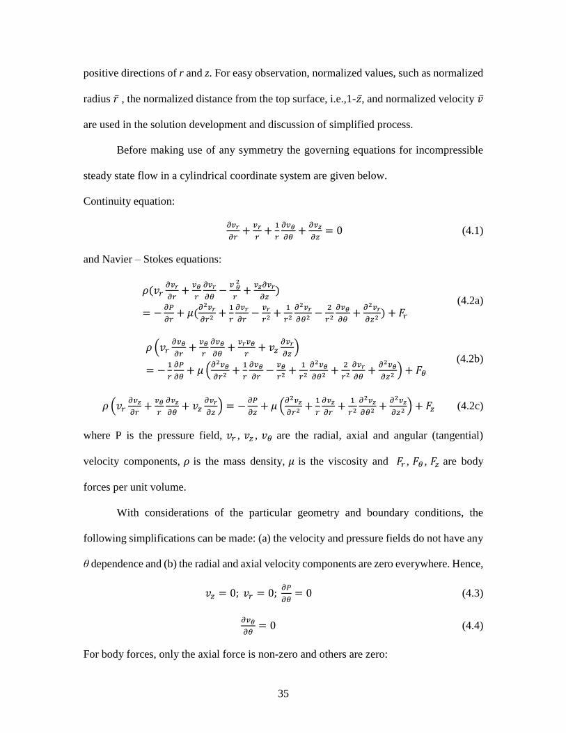
positive directions of r and z. For easy observation, normalized values, such as normalized

radius �̅� , the normalized distance from the top surface, i.e.,1-𝑧̅, and normalized velocity �̅�

are used in the solution development and discussion of simplified process.

Before making use of any symmetry the governing equations for incompressible

steady state flow in a cylindrical coordinate system are given below.

Continuity equation:

𝜕𝑣𝑟

𝜕𝑟+

𝑣𝑟

𝑟+

1

𝑟

𝜕𝑣𝜃

𝜕𝜃+

𝜕𝑣𝑧

𝜕𝑧= 0 (4.1)

and Navier – Stokes equations:

𝜌(𝑣𝑟𝜕𝑣𝑟

𝜕𝑟+

𝑣𝜃

𝑟

𝜕𝑣𝑟

𝜕𝜃−

𝑣 𝜃2

𝑟+

𝑣𝑧𝜕𝑣𝑟

𝜕𝑧)

= −𝜕𝑃

𝜕𝑟+ 𝜇(

𝜕2𝑣𝑟

𝜕𝑟2 +1

𝑟

𝜕𝑣𝑟

𝜕𝑟−

𝑣𝑟

𝑟2 +1

𝑟2

𝜕2𝑣𝑟

𝜕𝜃2 −2

𝑟2

𝜕𝑣𝜃

𝜕𝜃+

𝜕2𝑣𝑟

𝜕𝑧2 ) + 𝐹𝑟

(4.2a)

𝜌 (𝑣𝑟𝜕𝑣𝜃

𝜕𝑟+

𝑣𝜃

𝑟

𝜕𝑣𝜃

𝜕𝜃+

𝑣𝑟𝑣𝜃

𝑟+ 𝑣𝑧

𝜕𝑣𝑟

𝜕𝑧)

= −1

𝑟

𝜕𝑃

𝜕𝜃+ 𝜇 (

𝜕2𝑣𝜃

𝜕𝑟2 +1

𝑟

𝜕𝑣𝜃

𝜕𝑟−

𝑣𝜃

𝑟2 +1

𝑟2

𝜕2𝑣𝜃

𝜕𝜃2 +2

𝑟2

𝜕𝑣𝑟

𝜕𝜃+

𝜕2𝑣𝜃

𝜕𝑧2 ) + 𝐹𝜃

(4.2b)

𝜌 (𝑣𝑟𝜕𝑣𝑧

𝜕𝑟+

𝑣𝜃

𝑟

𝜕𝑣𝑧

𝜕𝜃+ 𝑣𝑧

𝜕𝑣𝑟

𝜕𝑧) = −

𝜕𝑃

𝜕𝑧+ 𝜇 (

𝜕2𝑣𝑧

𝜕𝑟2 +1

𝑟

𝜕𝑣𝑧

𝜕𝑟+

1

𝑟2

𝜕2𝑣𝑧

𝜕𝜃2 +𝜕2𝑣𝑧

𝜕𝑧2 ) + 𝐹𝑧 (4.2c)

where P is the pressure field, 𝑣𝑟 , 𝑣𝑧 , 𝑣𝜃 are the radial, axial and angular (tangential)

velocity components, 𝜌 is the mass density, 𝜇 is the viscosity and 𝐹𝑟 , 𝐹𝜃 , 𝐹𝑧 are body

forces per unit volume.

With considerations of the particular geometry and boundary conditions, the

following simplifications can be made: (a) the velocity and pressure fields do not have any

θ dependence and (b) the radial and axial velocity components are zero everywhere. Hence,

𝑣𝑧 = 0; 𝑣𝑟 = 0; 𝜕𝑃

𝜕𝜃= 0 (4.3)

𝜕𝑣𝜃

𝜕𝜃= 0 (4.4)

For body forces, only the axial force is non-zero and others are zero:

36

𝐹𝑟 = 0; 𝐹𝜃 = 0; 𝐹𝑧 = −𝜌𝑔 (4.5)

Substituting (4.3), (4.4), and (4.5) into (4.2), the governing equations are reduced to

𝜌 (−𝑣𝜃

2

𝑟) = −

𝜕𝑃

𝜕𝑟 (4.6)

𝜕2𝑣𝜃

𝜕𝑟2 +1

𝑟

𝜕𝑣𝜃

𝜕𝑟−

𝑣𝜃

𝑟2 +𝜕2𝑣𝜃

𝜕𝑧2 = 0 (4.7)

−𝜕𝑃

𝜕𝑧+ 𝐹𝑧 = 0 (4.8)

It is worth noting that viscosity does not enter into the above governing equations. Hence,

the resulting solutions are independent of the viscosity for this special case.

Since 𝑣𝜃 is a function of r and z, the method of separation of variables can be used

to get:

𝑣𝜃 = 𝑈(𝑟)𝑊(𝑧) (4.9)

where 𝑈(𝑟) and 𝑊(𝑧) are functions to be determined. Substituting (4.9) into (4.7) and re-

arrange it to get

𝑑2𝑈

𝑑𝑟2 +1

𝑟

𝑑𝑈

𝑑𝑟−

𝑈

𝑟2

𝑈= −

𝑑2𝑊

𝑑𝑧2

𝑊= −𝜆2 (4.10)

where 𝜆 is a constant.

Now introducing the following non-dimensional quantities:

r̅ =𝑟

𝑅, 𝑢 =

𝑈

𝑅𝜔, �̅�𝜃 = 𝑢𝑊, 𝑧̅ =

𝑧

𝐻, �̅� = 𝜆𝑅 (4.11)

where R is the radius of the process chamber, 𝜔 is the angular speed, and H is the height

of the chamber. Two equations below can be derived from (4.10) after these quantities are

substituted into equation (4.10)

d2𝑊

𝑑𝑧2̅̅̅̅ − (𝐻

𝑅)

2

�̅�2𝑊 = 0 (4.12)

�̅�2 𝑑2𝑢

𝑑𝑟2̅̅̅̅ +�̅�𝑑𝑢

𝑑�̅�+ (�̅�2�̅�2 − 1)𝑢 = 0 (4.13)

37

The equation (4.12) is a second time differential equation and its general solution is

𝑊(𝑧̅) = 𝑐1exp (𝐻�̅�

𝑅𝑧̅) + 𝑐2exp (−

𝐻�̅�

𝑅𝑧̅) (4.14)

where 𝑐1 and 𝑐2 are constants.

Equation (4.13) is a first-order Bessel equation and its general solution is

𝑢(�̅�) = 𝑐3𝐽1(�̅��̅�) + 𝑐4𝑌1(�̅��̅�) (4.15)

where 𝑐3 and 𝑐4 are constants and 𝐽1(𝑥) and 𝑌1(𝑥) are first-order Bessel functions of first

kind and second kind, respectively. The general solutions for the Bessel functions of first

kind can be expressed as

𝐽𝜐(𝑥) = ∑(−1)𝑚

𝑚!(𝑚+𝜐)! ∞𝑚=0 (𝑥/2)2𝑚+𝜐 (4.16)

where 𝜐 is a real value, meaning the order of the Bessel function, and m and k are integers.

The general solutions for the second kind,

𝑌1(𝑥) =2

𝜋 𝐽1(𝑥) (

ln 𝑥

2+ 0.5772) −

1

𝜋∑

(−1)𝑚(𝑥

2)

2𝑚

𝑚!(𝑚+1)! ∞𝑚=0 (∑

1

𝑘+1+ ∑

1

𝑘+1)𝑚−1

𝑘=0𝑚𝑘=0 (4.17)

Then the general solution for the tangential velocity �̅�𝜃 can be written as

�̅�𝜃 = 𝑊(𝑧̅)𝑢(�̅�) = (𝑐1exp (𝐻�̅�

𝑅𝑧̅) + 𝑐2exp (−

𝐻�̅�

𝑅𝑧̅) )(𝑐3𝐽1(�̅��̅�) + 𝑐4𝑌1(�̅��̅�) (4.18)

As described before, the contact between the fluid and chamber internal wall is non slip.

So the boundary conditions for the normalized quantities are

�̅� = 0, �̅�𝜃 = 0 (4.19a)

�̅� = 1, �̅�𝜃 = 0 (4.19b)

𝑧̅ = 0, �̅�𝜃 = 0 (4.19c)

𝑧̅ = 1, �̅�𝜃 = �̅� (4.19d)

Imposing condition (4.19a) to (4.18),

�̅� = 0, �̅�𝜃 = 𝑊(𝑧̅)𝑈(0) = 0 (4.20)

38

If (4.20) is true for any 𝑧̅, then 𝑢(0) must be zero, namely

c3𝐽1(0) + 𝑐4𝑌1(0) = 𝑐3 ∗ 0 + 𝑐4 ∗ (−∞) = 0 (4.21)

Solve (4.21),

c4 = 0 (4.22)

Similarly, from (4.19b),

c3𝐽1(�̅�) = 0 (4.23)

So the value of �̅� can be determined. There are infinite number of zero roots for �̅�.

Then 𝑢(�̅�) can be written as

𝑢(�̅�) = 𝑐3𝐽1(�̅�𝑟)̅ (4.24)

From (4.19c), we can get

𝑊(0) = 𝑐1 + 𝑐2 = 0 (4.25)

Let 𝑐1 = −𝑐2 = 𝑐5 then

𝑊(𝑧̅) = 𝑐5sinh (𝐻�̅�

𝑅𝑧̅) (4.26)

Let 𝑐 = 𝑐3𝑐5 and rewrite (4.18)

�̅�𝜃 = 𝑐sinh (𝐻�̅�

𝑅𝑧̅) 𝐽1(�̅��̅�) (4.27)

Since there are an infinite number of eigenvalues �̅�, �̅�𝜃 can be written as

�̅�𝜃 = ∑ 𝑐𝑛 sinh (𝐻�̅�𝑛

𝑅𝑧̅)∞

𝑛=1 𝐽1(�̅�𝑛�̅�) (4.28)

Apply boundary condition (4.19d) to (4.28),

�̅� = ∑ 𝑐𝑛 sinh (𝐻�̅�𝑛

𝑅𝑧̅)∞

𝑛=1 𝐽1(�̅�𝑛�̅�) (4.29)

The Bessel function has one of orthogonality properties as follows [127]

∫ �̅�𝐽11

0(�̅�𝑗�̅�)𝐽1(�̅�𝑘�̅�)𝑑�̅� = {

0, 𝑗 k

1

2[

𝑑𝐽1(𝑥)

𝑑𝑥]

𝑥=�̅�𝑘

2

, 𝑗 = 𝑘 (4.30)

39

The solved constants are

cm =2

�̅�𝑚sinh(𝐻�̅�𝑚

𝑅)𝐽2(�̅�𝑚)

(4.31)

The final solution for the normalized tangential velocity is

�̅�𝜃 = ∑2 sinh(

𝐻�̅�𝑛𝑅

�̅�)𝐽1(�̅�𝑛�̅�)

�̅�𝑛sinh(𝐻�̅�𝑛

𝑅)𝐽2(�̅�𝑛)

∞𝑛=1 (4.32)

It is seen that the analytical solution is expressed in terms of a series of infinite

number of terms. A convergence analysis of the series has shown that a converged value

can be achieved very quickly except right on the rotating surface. In subsequent sections,

the analytical solution is calculated using the first fifty terms to ensure a good convergence.

∫ �̅�𝐽11

0(�̅�𝑗�̅�)𝐽1(�̅�𝑘�̅�)𝑑�̅� = {

0, 𝑗 k

1

2[

𝑑𝐽1(𝑥)

𝑑𝑥]

𝑥=�̅�𝑘

2

, 𝑗 = 𝑘 (4.30)

The solved constants are

cm =2

�̅�𝑚sinh(𝐻�̅�𝑚

𝑅)𝐽2(�̅�𝑚)

(4.31)

The final solution for the normalized tangential velocity is

�̅�𝜃 = ∑2 sinh(

𝐻�̅�𝑛𝑅

�̅�)𝐽1(�̅�𝑛�̅�)

�̅�𝑛sinh(𝐻�̅�𝑛

𝑅)𝐽2(�̅�𝑛)

∞𝑛=1 (4.32)

It is seen that the analytical solution is expressed in terms of a series of infinite

number of terms. A convergence analysis of the series has shown that a converged value

can be achieved very quickly except right on the rotating surface. In subsequent sections,

the analytical solution is calculated using the first fifty terms to ensure a good convergence.

40

4.3 Numerical Modeling

A three-dimensional CFD simulation of the simplified process was carried out

without using the simplifications taken explicitly in obtaining the analytical solution. The

simulation is performed in a rectangular Cartesian coordinate system with the same origin

as the cylindrical coordinate system for the analytical solution.

Using the indicial notation, in which Latin indexes have ranges of 1, 2 and 3, the

rectangular Cartesian coordinates are represented by xi and the velocity components are

represented by vi. Now the governing equations, namely the continuity equation and the

Navier-Stokes equations, for incompressible steady state flow are given in Cartesian

coordinates by, respectively,

𝜕𝑣𝑖

∂𝑥𝑖= 0 (4.33)

𝜌𝑣𝑖𝜕𝑣𝑗

𝜕𝑥𝑖= −

𝜕𝑃

𝜕𝑥𝑗+ 𝜇 (

𝜕2𝑣𝑖

𝜕𝑥𝑖𝜕𝑥𝑗) + 𝐹𝑗 (4.34)

The boundary conditions, namely that the top surface rotates at the angular speed

ω and the other surfaces are stationary, are the same as for the analytical solution.

The CFD simulation was carried out only considering the fluid part with the

following specific parameter values: =0.5 rpm, =2.5 Pa-s, R=19 mm and H=44 mm,

which are the same as those used in experiment. Figure 4.3 shows the converged

computation grid. It was found that a high mesh density close to the rotating surface, i.e.

the die-fluid interface, is necessary to capture the high velocity gradients. Also, for the

regions close to the other walls, finer mesh is needed. Boundary layer mesh which is finer

is shown in Figure 4.3 (b). A numerical convergence analysis of the simulation solution

was conducted. Based on original mesh, every cell was refined in three directions, i.e. split

into eight cells. Then the numerical predictions using the refined mesh was compared with

41

that using original mesh. If the relative different is less 5%, both mesh grids can be

considered converged mesh. In fact, right now the PC is powerful and able to handle

considerable number of cells with ease. The CFD simulation predictions discussed below,

which are presented together with the analytical solution for comparison purposes, are from

the converged simulation solution.

Finite control volume method was used to discretize the computational domain and

ANSYS FLUENT was used to solve the governing equations. A second order discretization

scheme was chosen for the pressure and a second order upwind scheme for the momentum

equations. The SIMPLE algorithm was used for the pressure-velocity coupling [128]. A

convergence could be reached easily for this problem.

4.4 Comparisons and Discussions

Converged simulation predictions are now presented together with the analytical

solution for comparison purposes. The comparisons of CFD simulation predictions and the

analytical solution of the tangential velocity along both axial and radial directions are

shown in Figure 4.4. All values in the figures are normalized, including the geometric

(a) (b)

Figure 4.3 (a) Mesh, (b) details for mesh boundary layer.

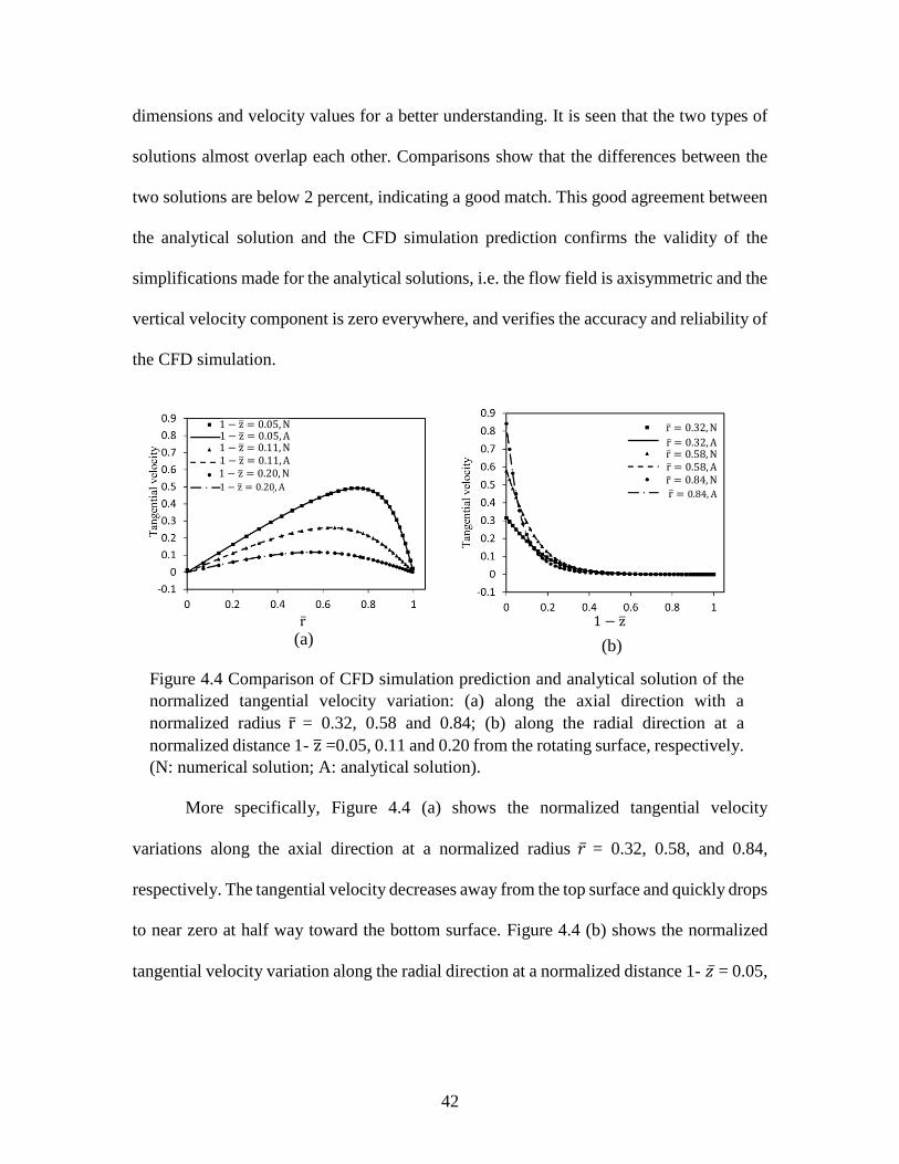
42

dimensions and velocity values for a better understanding. It is seen that the two types of

solutions almost overlap each other. Comparisons show that the differences between the

two solutions are below 2 percent, indicating a good match. This good agreement between

the analytical solution and the CFD simulation prediction confirms the validity of the

simplifications made for the analytical solutions, i.e. the flow field is axisymmetric and the

vertical velocity component is zero everywhere, and verifies the accuracy and reliability of

the CFD simulation.

More specifically, Figure 4.4 (a) shows the normalized tangential velocity

variations along the axial direction at a normalized radius �̅� = 0.32, 0.58, and 0.84,

respectively. The tangential velocity decreases away from the top surface and quickly drops

to near zero at half way toward the bottom surface. Figure 4.4 (b) shows the normalized

tangential velocity variation along the radial direction at a normalized distance 1- 𝑧̅ = 0.05,

r̅ 1 − z̅

(a) (b)

Figure 4.4 Comparison of CFD simulation prediction and analytical solution of the

normalized tangential velocity variation: (a) along the axial direction with a

normalized radius r̅ = 0.32, 0.58 and 0.84; (b) along the radial direction at a

normalized distance 1- z̅ =0.05, 0.11 and 0.20 from the rotating surface, respectively.

(N: numerical solution; A: analytical solution).

1 − z̅ = 0.05, N 1 − z̅ = 0.05, A

1 − z̅ = 0.11, A 1 − z̅ = 0.11, N

1 − z̅ = 0.20, N 1 − z̅ = 0.20, A

r̅ = 0.32, N

r̅ = 0.32, A

r̅ = 0.58, A r̅ = 0.58, N

r̅ = 0.84, N

r̅ = 0.84, A

43

0.11 and 0.20, respectively, from the rotating surface. It is seen that the tangential velocity

is largest at an intermediate radius toward the cylindrical wall of the process chamber.

A full view of the velocity field variation can be seen clearly from the contour plot

of the tangential velocity on the Zr plane in Figure 4.5, in which normalized contour values

are shown on a full rectangular cross-section of the process chamber. It is obvious that the

velocity has the largest values in the upper left and upper right regions (these two regions

are symmetric about the vertical centerline, which is the axis of the cylindrical chamber).

These two regions, which are bounded from below by the 0.10 contour, occupy about 20%

of the whole flow domain. In these two regions, the normalized velocity magnitude ranges

mainly from 0.1 to 1, and in the rest of the chamber, the velocity magnitude is below 0.1.

In other words, the dominant material flow activity occurs in a small region of the chamber,

while in the rest of the chamber material flow is very limited. Also the velocity magnitude

is relatively small along the cylindrical axis.

z

r O

Figure 4.5 A contour plot of

the tangential velocity.

44

Generally speaking, the distribution of the velocity field is expected to be affected

by the viscosity of the fluid. However, from the analytical solution, it is seen that the

velocity field is independent of viscosity. This independence is a consequence of the use

of a Newtonian fluid, which has a constant viscosity. For non-Newtonian fluids, the

viscosity is not a constant (e.g. with dependence on temperature and strain rate) and is

expected to affect the velocity distribution.

Since the CFD simulation predictions have been shown earlier to be almost the

same as the analytical solution for the modified process, and the analytical solution

provides more mathematical convenience, experimental validation of the analytical

solution and CFD simulation predictions is performed below in the form of comparisons

between the analytical solution and experimental measurements.

The comparisons between analytical solution and experiment measurements are

shown in Figure 4.6. The analytical solution is derived from equation (4.32) by using the

measured (�̅�, 1- 𝑧̅) coordinates of the marker particles since these two coordinates for a

given particle are found to change with time in the experiment. It is noted that, in the perfect

world of the analytical solution, the particles are required to keep these two coordinates

constant. This is believed to be the main reason for the differences between the analytical

solution and the experimental measurements.

In Figure 4.6, the experimental measurements are from six marker particles (#1~#6

in the figures) that were tracked during the experiment. The positions of the particles were

recorded every 10 seconds. The measured velocity varied with time due to the fact that

during the experiment the particles oscillated not only up and down, but also along the

45

(a) (b)

(c) (d)

Figure 4.6 Comparisons of the analytical solution and experimental

measurements of the normalized tangential velocity variation with time for (a)

marker particle #1, (b) marker particle #2, (c) marker particle #3, (d) marker

particle #4, (e) marker particle #5, and (f) marker particle #6, respectively.

(e) (f)

46

radial direction. That is, as noted earlier, the (�̅�, 1- 𝑧̅) coordinates of the particles changed

with time, as shown in Figure 4.7.

It is seen from Figure 4.6 that the velocity values from the analytical solution and

experimental measurements are very close. The qualitative trends are the same and the

quantitative differences are small. Most the quantitative differences are less than 6% in

Figure 4.6(a) - (e) and less than 12% in Figure 4.6(f). The main factors that may have

contributed to the differences during experiments include the wobbling motion of the die

due to misalignment of the die axis with the drive shaft. Improvements will be made in the

future to minimize experimental errors. Nonetheless, the current comparisons between the

analytical solution and experimental measurements show a good agreement, which serves

as an evidence for experimental validation of the analytical solution and CFD simulation

predictions.

Figure 4.7 Variation of (a) height and (b) radius with time for the six markers

particles.

(a) (b)

r̅

1−

z̅

47

4.5 Summary and Conclusions

In this chapter, a simplified model has been studied and it is to mimic the material

flow features during friction extrusion process. The model includes a rotating die under a

Newton fluid in a chamber. The Reynolds number is equal to that estimated in the friction

extrusion process. Due to the regularity of the problem, an analytical solution has been

derived based on some reasonable assumptions. A CFD simulation of the problem also has

been performed but without any assumptions. A very good agreement between the

analytical solution and the numerical predictions can be observed and the assumptions

made in the derivation of the analytical solution are verified. The numerical solution also

was compared with experimental measurements made through a DIC system on small solid

particles in the fluid. The comparisons show that the velocity qualitative trends are the

same and the quantitative differences are small. The good agreement between the analytical

solution, the numerical predictions, and experimental measurements serve as an evidence

for experimental validation of the analytical solution and CFD simulation predictions.

48

CHAPTER 5 HEAT TRANSFER MODELING

In this chapter, a heat transfer numerical model has been developed to study the

heat flow during the friction extrusion process. The heat transfer model will be employed

in a more comprehensive numerical model for further investigations. In this model the heat

source is decoupled from friction or plastic deformation and the heat transfer phenomenon

during friction extrusion process is investigated by a pure thermal model. As a first step,

without material flow, it is more convenient to study the heat transfer phenomenon in

friction extrusion process. The pure thermal model, as “pure” implies, means only heat

transfer is simulated and the precursor material in the chamber and all tools are treated as

solids. Only the equation of the conservation of energy is needed to solve. The goal of the

pure thermal model is to obtain temperature fields, to know the temperature distribution,

and to determine thermal boundary conditions.

Although the material flow is very strong in the friction extrusion process under the

die-precursor interface, the pure thermal model is expected to capture the temperature field

reasonably without consideration of material flow. There are three aspects that can account

for it. First, the region with strong material flow under the die-precursor interface is small.

That can be seen from the cross section of the remnant disk in the chamber after experiment

as mentioned in Chapter 2. Second, in the strong material flow region, the tangential

velocity is almost dominant due to high rotation speed of the die and the radical velocity is

expected relatively small. As a result, the heat transfer due to material flow is mainly

49

radical. Third, the aluminum alloy 6061 has much higher heat conductivity so that the

conduction heat transfer is dominant over the heat convection due to material flow.

To study the heat transfer phenomenon, heat generation source is always of interest.

In friction extrusion process, the heat generation comes from two parts, i.e., the friction

between the die and the precursor material in the chamber and material plastic deformation.

So far, it is very difficult to determine the percentages of these two heat sources during the

process and to know how they are distributed. Some simplifications or assumptions must

be made. Numerical studies on the similar process, the friction stir welding process, as

described in the literature review in Chapter 3, include interface influx on the friction

interface, viscous dissipation, and combination of them [92]. The heat generation power is

estimated based on yield stress or fitted by comparing experimental measurements. Since

friction stir welding is a steady state process except the beginning and ending, by using

these methods good approximations can be easily obtained. However, unlike friction stir

welding process, friction extrusion process shows apparent transient state features for heat

transfer. The heat generation power varies during friction extrusion process. Consequently,

difficulties occur when adopting the methods used in friction stir welding to approximate

the heat generation rate in friction extrusion process. To avoid such difficulties, the

mechanical power during friction extrusion experiment can be used to relate the heat

generation power. So in this pure thermal model, the heat generation rate is a function of

the mechanical power. The details pertaining the pure thermal model are described in the

following subsections.

50

5.1 Model Description

In order to capture the heat transfer phenomenon in the friction extrusion

experiment, the heat transfer model considers all parts involved in friction extrusion

process, such as the die, the chamber, the aluminum alloy sample, the back plate and the

supporting table. Compared with the chamber and the sample, the die, the back plate and

the table have relative larger sizes. Considering the relative large volumes of them and

lower conductivities, it is expected that overall temperatures of them don’t change much

although the heat flows into them continuously. However, the temperature definitely

increases drastically in the regions where it is close to the aluminum alloy sample.

Apparently, it is not necessary to simulate the whole bodies. The faraway areas can be

excluded since the temperature almost retains the same. Thus a lot of computing efforts

can be saved. The sizes of the bodies of the die, the back plate, and the table included in

the model should be chosen carefully so that they can represent the effect of the whole

bodies. Various sizes of these parts are tried and their results are compared. The final sizes

are determined if larger sizes would not affect the predictions pronouncedly. In addition,

the temperatures of these select parts are not high, the predictions are not sensitive to the

boundary conditions on the boundaries of the parts. Other than the mentioned

approximations to the die, the back plate and the table, the actual geometrical dimensions

of the experimental setup are used in the thermal model.

Similar to non-flow based thermal models for friction stir welding [90], this is a

pure thermal model in which the material flow is not modeled. As such, considering the

characteristics of the problem, such as the geometry, the governing equation, and the

boundary conditions, a two-dimensional axisymmetric model is found appropriate for the

51

process. Utilization of the axisymmetry saves computing efforts significantly since only

half of the cross-sectional area along the axis of symmetry is needed for the geometry.

The finite volume method is used to discretize the computational domain. The mesh

is shown in Figure 5.1. The aluminum alloy has a radius of 12.75 mm. The final sizes for

the back plate and the table are the same, 50 mm in radius. A grid with a cell size of 0.5

mm is used. The time step is 0.05 second. Convergence analysis has been conducted and

the grid used in this work is converged. The commercial code ANSYS FLUENT is used to

carry out the computations.

Since this is to study the heat transfer, the most key factor is heat generation. So

the heat generation is first discussed. As in the work done by Schmidt et al. [92], three

contact conditions are defined: sliding condition that the contact shear stress is smaller than

the aluminum sample yield shear stress, sticking condition that the aluminum sample

Figure 5.1 The

thermal model grid.

Figure 5.2 A cross section of the remnant

aluminum alloy sample after etching.

52

surface sticks to the moving tool surface segment, and partial sliding/sticking condition

that is a mixed state of the former two states. During the friction extrusion process, all these

three contact conditions may happen. In the first few seconds, the sliding condition occurs

because the yield shear stress of the aluminum sample is larger than the stress under the

compression and torque. The z-force applied on the die is smaller in the first few seconds,

which also makes it easily slide. The continued friction between the die and the aluminum

alloy sample generates heat and temperature near the sliding interface increases fast. The

rising temperature causes the decrease of the strength of the aluminum alloy sample locally.

At a certain point, the strength lowers down to the friction stress, the second condition, i.e.

partial sliding/sticking, occurs. After yield, the material has large plastic deformation.

When the material at the interface becomes softer, the degree of sticking increases. Sticking

or close sticking may happen when the material is soft enough at high temperature.

Obviously, both friction and plastic deformation happens during the friction

extrusion process, and both of them generate heat. The heat generation in terms of friction

is a surface heat flux and it is a volume flux for plastic deformation. In the pure thermal

models of FSW without consideration of material flow, Chao et al. [92] used trial and error

method to find total power input, Khandkar et al. [87] correlated mechanical power to heat

generation, and Schmidt and Hattel [93] estimated heat generation only by a surface flux

based on an assumption that the shear layer or deformation zone is very thin and uniform.

The surface heat flux model works well for FSW. However, in the friction extrusion

experiment, after the start of extrusion, the deformation zone or shear layer is not relatively

thin. Experimental observations show that at the end of extrusion the thickness of

deformation zone was about 4 mm on average compared with the height of sample 19 mm

53

in a friction extrusion experiment. Figure 5.2 shows a cross section of remnant of the

aluminum alloy sample after experiment after etching. The thickness of the deformation

area is not thin at all. Thus both a surface flux and a volume flux should be considered to

model the heat generation in terms of friction and volume deformation respectively.

However, there are some difficulties if a surface heat flux is used in the numerical

modeling, especially when the surface is the interface of two bodies, like the current work.

First, it will introduce difficulties to boundary condition settings. When two bodies are in

contact, the heat transfers between these two bodies through heat conduction. There may

be thermal resistance at the interface. At the interface, it is thermally coupled. So the

temperature contours are continuous and there is no jump. If the surface heat flux is used,

the conduction heat transfer between the two bodies will be broken and both the two

surfaces of the bodies must be assigned heat fluxes. In that case, it’s not thermally coupled

anymore and the temperature is not continuous. Clearly, the surface heat flux will bring

temperature discontinuity in temperature sensitive area. Second, some assumptions are

needed for the surface flux. There are two bodies, the die and the aluminum alloy sample,

and the contact surfaces are assigned surface fluxes. This means the friction heat generation

needs to be split into two parts. However, how to split is unknown and some assumptions

must be made. Even more, the percentage of the frictional heat generation is not known.

Third, if the surface heat flux is used, the distribution of heat generation rate on the surfaces

needed to be determined. Usually, it is assumed that the friction coefficient is uniform.

Then the friction heat generation over an infinitesimal interface area dA can be written as

𝑑𝑞 = 𝜂𝑃𝑣′𝑑𝐴 (5.1)

54

where 𝑣′ is the relative velocity, 𝜂 is the friction coefficient, and 𝑃 is the pressure. Thus,

another assumption is needed.

To overcome the shortages and to avoid the difficulties, a volume heating method

with compensation of the surface heat flux effect is proposed to approximate the heat

generation. Compared with surface heat fluxes, the volume heat source doesn’t have the

disadvantages listed above. It is proposed that heat generation is represented by a volume

heat source in a material layer in the sample under the interface where the material

undergoes extensive flow and severe plastic deformation. The height of the layer is

determined based on experimental observations of the material flow region in the sample.

As described in Chapter 2, a thin marker wire was inserted into the sample in order to

investigate material flow in friction extrusion. After the friction extrusion experiment,

observations of marker material positions in the remnant of the sample in the chamber

revealed that the depth of the material flow region in the remnant is about 4.5 mm at one

third of the sample radius from the center and it is smaller near the edge of the sample. As

an approximation, and for simplicity, a material layer next to the interface with a uniform

height of 4 mm is taken as the layer with a volume heating source.

One common limitation of non-flow based thermal models, such as the present

model and those in the literature for the related process of friction stir welding, is that the

spatial distribution of the heat source must be approximated based on certain

simplifications and idealizations. At this time, due to the lack of information from the

friction extrusion literature, the heat source distribution in the present study is assumed

based on considerations from the literature for friction stir welding and on observations of

material flow patterns in friction extrusion process experiments, as discussed earlier.

55

First, it is noted that the radial distribution of frictional surface heat flux is often

approximated by a linear distribution in the friction stir welding literature, resulting from

the product between a shear stress created by a uniform tool pressure and a tangential

velocity created by rigid tool rotation. For simplicity, and as a first order approximation,

this linear distribution in the radial direction is adopted in the present study in the volume

heat source method, since the volume heat source is in a region immediately adjacent to

the die-sample interface.

Second, in the vertical direction (which is the axial direction of the cylindrical

sample), it is expected that plastic deformation is greater closer to the die-sample interface,

thus more heat is expected to be generated closer to the interface. In addition, the friction

heat generation occurs at the interface. For simplification again, a linear distribution along

the vertical direction is assumed for the volume heat source.

Figure 5.3 The sample geometry

and coordinates.

H

h

z = 0

z+dz

R

z θ

r+dr r

r

z

56

Based on the above simplifications, the heat generation rate in the volume heat

source method can be expressed as below

𝑞 = 𝑚(𝑧 − ℎ)𝑟 (5.2)

where m is a power-related quantity to be determined, q is the volumetric heat generation

rate, and h is the height of the sample without heat source (see Figure 5.3 for a schematic

of the sample geometry and the coordinate system).

The total heat generation power can be obtained by integration over the volume

heating layer from 𝑧 = ℎ to 𝑧 = 𝐻 (see Figure 5.3):

𝑄𝑡𝑜𝑡𝑎𝑙 = ∫ ∫ ∫ 𝑞 ∙ 𝑟𝑑𝑧𝑑𝑟𝑑𝜃𝐻

ℎ

𝑅

0

2𝜋

0= ∫ ∫ ∫ 𝑚𝑟(𝑧 − ℎ) ∙ 𝑟𝑑𝑧𝑑𝑟𝑑𝜃

𝐻

ℎ

𝑅

0

2𝜋

0=

1

3𝑚𝜋(𝐻 − ℎ)2𝑅3

(5.3)

In the current thermal model, Qtotal is set to equal to the mechanical power input in the

friction extrusion experiment, which was recorded in the experiment as a function of time.

From equation (5.3), the quantity m can be determined, which can be substituted

into equation (5.2). Finally, the volumetric heat generation rate per unit volume is given by

𝑞 =3𝑄𝑡𝑜𝑡𝑎𝑙

𝜋(𝐻−ℎ)2𝑅3 𝑟(𝑧 − ℎ) (5.4)

This expression is implemented into the code ANSYS FLUENT through a user defined

function.

In the model it is assumed that all of the mechanical work is dissipated in the billet,

i.e. the aluminum alloy sample, thereby contributing to heating of the billet. This is

justified based on the following:

1. The extrusion apparatus does not deform plastically during the process, all

deformation, hence heating, occurs in the billet.

57

2. The primary mechanism of storage of deformation energy in metals is the

production of dislocations. In a highly deformed material, the maximum expected

dislocation density is on the order of 1016/m2. The maximum possible total stored

deformation energy in the billet is then, the product of the billet volume, the

dislocation density, and the dislocation line energy. For the present situation, this

equates to approximately 77 J while the total energy input during the simulation is

on the order of 80 KJ.

3. Evidently, the maximum possible stored deformation energy is a small fraction of

the mechanical work supplied. Additionally, previous work has demonstrated that

the extruded wire and the remaining billet material are in a fully recrystallized

condition indicating that the stored dislocation energy will be much less than the

maximum.

Therefore, for the present experiment (and likely most any other friction extrusion

experiment) it is justified to assume that all of the mechanical work contributes to heating.

5.2 Governing Equations

Numerical simulations are using numerical methods to solve governing equations

under certain boundary conditions. The considerable development of numerical methods

enables accurate predictions about field variables, such as stress, strain, velocity,

temperature, material path lines, etc., if boundary conditions are known or estimated

properly. In numerical modeling, the description of motion is chosen depending on the

problem solved. The governing equations may be not same for a different choice. For heat

transfer problem, if there is not material flow, the heat is transferred in solids or fluids in

the form of diffusion or conduction. The current pure thermal model is an example. The

58

governing equation is the conservation of energy. According to the first law of

thermodynamics, the sum of work and heat in a system results in the change of the energy

of the system. With indicial notation (i = 1, 2, and 3) the equation can be expressed in

Cartesian coordinates as

𝜌𝑐𝑝𝜕𝑇

𝜕𝑡=

𝜕

𝜕𝑥𝑖(𝑘

𝜕𝑇

𝜕𝑥𝑖) + 𝑞 (5.5)

where 𝜌 is density, 𝑐𝑝 is the specific heat, 𝑘 is conductivity, 𝑥𝑖 are coordinates, and 𝑞 is

heat generation source given by equation (5.4). For a two-dimensional axisymmetric

problem, the transient conduction equation can be written as

1

𝑟

𝜕

𝜕𝑟(𝑘𝑟

𝜕𝑇

𝜕𝑟) +

𝜕

𝜕𝑧(𝑘

𝜕𝑇

𝜕𝑧) + 𝑞 = 𝜌𝑐𝑝

𝜕𝑇

𝜕𝑡 (5.6)

where 𝑟 and 𝑧 are the coordinates.

5.3 Initial and Boundary Conditions

Numerical simulations are to solve governing equations, which must be satisfied

everywhere inside the computational field, combined with some constitutive relations of

the materials and certain initial and boundary conditions by numerical methods such as

finite element methods and computational fluid dynamic methods. Usually the reliability

of the results of numerical simulations depends on the initial and boundary conditions given

that the current computer is powerful and numerical methods have obtained good

developments. If the initial and boundary conditions imposed in the numerical modeling

represent the real ones, the numerical predictions can be very accurate for some problems.

So does the heat transfer problem to be solved in current work.

There are three different modes of heat transfer, the conduction, the convection,

and the radiation. Heat transfer by conduction arises from temperature gradient in a

material or between materials. In the current work, conduction is the mode in the system.

59

When two solids are put together, heat transfer between them through conduction may not

be perfect as in a single body. There is thermal resistance between them due to not perfect

contact. The convection is the heat transfer between a solid surface and the adjacent fluid

medium. If the fluid is flowing, it is forced convection and the heat transfer is quicker. The

heat transfer rate can be expressed by

𝑞′ = ℎ𝑐Δ𝑇 (5.7)

where 𝑞′ is the heat transfer rate, ℎ𝑐 is the convection coefficient, and Δ𝑇 is the

temperature difference between the solid body and the adjacent fluid. The radiation occurs

between two objects which are placed in a finite distance apart. As if there is temperature

difference between the two objects, there is radiation between them. The heat transfer rate

through radiation is given by

𝑞′ = 𝜖𝛽(𝑇14 − 𝑇2

4） (5.8)

where 𝜖 is the emissivity, 𝛽 is the Stefan-Boltzmann constant, and 𝑇1 and 𝑇2 are the

objects’ temperatures. In this work, since the estimated radiation rate is very small

compared with the mechanical power, the radiation is neglected in the modeling.

At the beginning of the friction extrusion process experiment, the temperature of

all parts was the same as the lab room temperature, so the initial condition in the thermal

model is set at the lab room temperature of 295 K.

When the temperatures of the extrusion chamber, the die, and the back plate

increase, a part of the heat will flow into the air through convective heat transfer on the

surfaces which are exposed to the air. In the model, a convection boundary is used to model

such heat transfer. The convection coefficient for surfaces which are stationary in the

process is 5 W/m2-K, which is the typical value for natural convection between carbon

60

steel and air. For the moving surfaces, such as surfaces on the rotating die, two times the

typical value is used as an approximation to account for forced convection heat transfer.

In order to model the heat transfer process realistically, the back plate and the table

under the back plate are considered in the thermal model, as discussed earlier. Convection

boundary condition is also used on the outer surfaces of the back plate and the table. The

value used in the model is 10 W/m2-K. The dimensions of the back plate and the table

included in the thermal model are selected after a careful study of their effects. It is found

that, if the thickness of the table and the radial length of the back plate and the table in the

model are large enough, the model predictions are insensitive to the convection coefficient

value on the outer surfaces of the back plate and the table. Thus the assumed convection

boundary condition has little effect on the temperature field.

The connections between the sample and the back plate, between the chamber wall

and the back plate, and between the back plate and the table are taken to be perfect without

any thermal resistance. That is, these parts of the thermal system are considered thermally

coupled and in perfect contact. This approximation is reasonable due to the fact that during

the extrusion experiment the sample was under high pressure exerted by the extrusion die,

and that the chamber wall was tightly clamped on the back plate for prevention of slippage

between them.

The situation of contact between the sample and the chamber wall in the friction

extrusion experiment is more complicated. In the experiment, the sample and die diameter

was slightly smaller than the chamber inner diameter, so there was no friction between the

die and the chamber inner wall. However, there was a thin gap between the aluminum alloy

sample and the chamber inner wall, which was initially filled with air. The gap with air

61

could block heat transfer from the sample into the chamber wall. After the start of the

extrusion, the temperature and pressure in the sample increased drastically, and then a part

of the sample material was forced to flow into the gap according to experimental

observations. During the friction extrusion experiment, some material extruded out from

the gap was observed. Subsequently, the part of the gap where it was filled with the sample

materials made the heat transfer between the sample and the chamber wall easier. When

the experiment was finished, the gap was found to be completely filled by the sample

material based on experimental observations. The gap is expected to be filled up gradually.

However, the exact process through which the gap was filled is unknown and cannot be

determined in this pure thermal model. Nevertheless, the time when the gap started to be

filled in the experiment can be determined from recorded experimental data.

Figure 5.4 shows the die position as a function of time during the friction extrusion

experiment. In the first three seconds, the die moved downward from about 0.25 mm above

the top surface of sample. In the next period of t = 3 – 4.7 s, the die almost stayed at the

Figure 5.5 Torque and z force.

0

5

10

15

20

25

30

35

40

45

50

0

50

100

150

200

250

300

0 2 4 6 8 10 12 14

Z F

orc

e (k

N)

To

rque

(N-m

)

Time (s)

torquez force

Figure 5.4 Die position.

-3

-2.5

-2

-1.5

-1

-0.5

0

0 2 4 6 8 10 12 14

Die

Po

siti

on (

mm

)

Time (s)

62

same position. Then after t = 4.7 s, the die moved downward again. Figure 5.5 illustrates

the z force and the torque applied on the die, respectively, during the experiment. The non-

zero torque value in the first 0.2 s is meaningless due to a system bug which started to

record data from the end of the previous experiment. It is observed that the force and torque

both increased with time. In order to determine when the sample began to flow into the

initial gap between the sample and the chamber inner wall, an approximate analysis of the

stress state (see Figure 5.6) in the sample has been conducted. The normal and shear

stresses, σz and τ, can be approximated as follows

𝜎𝑧 =𝑧 𝑓𝑜𝑟𝑐𝑒

𝐴, 𝜏 =

2∙𝑡𝑜𝑟𝑞𝑢𝑒

𝜋𝑅3 (5.8)

where A and R are the cross section area and diameter of the cylinder, respectively.

Based on the equations and data, the stresses at different times can be estimated. At

t = 3 s, the z direction stress was σz = -28.3 MPa and the maximum shear stress on the cross

section occurred at the edge of the sample cylinder and it was about τmax =18.7 MPa. Thus

the maximum effective stress was σe = 53.9 MPa. The highest temperature is estimated at

Figure 5.6 Stress state (z-

vertical direction, r-radial

direction, and t-tangential

direction).

z

t

r

σz

τ

τ

σz O

63

323 K at that moment according to the temperature measurement at point 2, which was 305

K. The yield stress for sample (AA 6061) is more than 200 MPa at 323 K, so that the

sample material was not yielded yet at t = 3 s. Accordingly, during the period of t = 0 – 3

s, the die movement did not cause the sample material to flow into the gap since there was

no yielding.

At t = 4.7 s, the z direction stress was σz = -54.9 MPa and the maximum shear stress

on the cross section occurred at the edge of the sample cylinder and it was τmax =55.3 MPa.

Thus the maximum effective stress was σe = 146.2 MPa. The estimated highest temperature

is 573 K based on the temperature measurement at point 2, which was 497K at which the

yield stress is less than 138 MPa. At this moment, a part of the sample material began

yielding. Thus, it is seen that the die movement began to force the sample material to flow

into the gap from t = 4.7 s.

Table 5.1 Material Properties

Name Material Density

(kg/m3)

Specific Heat

(J/kg-K)

Thermal

Conductivity

(W/m-K)

Sample AA 6061 2,700 789.9+0.4959T 115.2+0.1594T

Die H13 steel 7,800 460 25

Chamber Wall O1 steel 7,800 460 33

Back Plate Al6xn steel 7,800 500 13

Table Carbon Steel 7,800 500 50

Again, since the current thermal model does not consider material flow nor elastic-

plastic deformation of the sample material, the exact manner in which the initial gap

between the sample and the chamber inner wall was filled cannot be determined. However,

based on the above estimates of the stress state, it is approximated in the thermal model

64

that the gap was filled gradually from t = 4.7 s to the start of extrusion of the wire at t = 10

s.

5.4 Material Properties

The range of temperature variation in the friction extrusion experiment was large,

approximately from 295 K to 848 K. The thermal properties of aluminum alloy are

sensitive to temperature variation, and thus temperature-dependent thermal properties are

considered in the thermal model. The materials and their properties used in the model are

listed in Table 1 based on data from reference [97].

5.5 Results and Discussions

5.5.1 Measurements and Validation

In the extrusion experiment, temperature variations were recorded at designated

locations using thermal couples. The measured temperature variations with time are plotted

in Figure 5.7. For validation purposes, temperature variations at the same locations that are

predicted by the thermal model are also shown in Figure 5.7. At t = 0, the die began to

rotate and there already was a vertical force of 2.2 kN exerted on the sample. The extrusion

of the wire started at about t = 10 second and ended at t = 27.7 s.

Generally, the comparisons show a good agreement between predicted and

measured temperature variations with time. Point 2 was in the extrusion die near the

die/sample interface. It can be seen from Figure 5.7(a) that the predicted temperature

variation at point 2 matches the experimental measurement very well, which indicates that

the heat transfer between the die and the sample has been modeled accurately. For the

predictions at points 3, 4, and 5, illustrated in Figure 5.7(b), there are small discrepancies

with experimental measurements. That might be caused by the uncertain effects of the

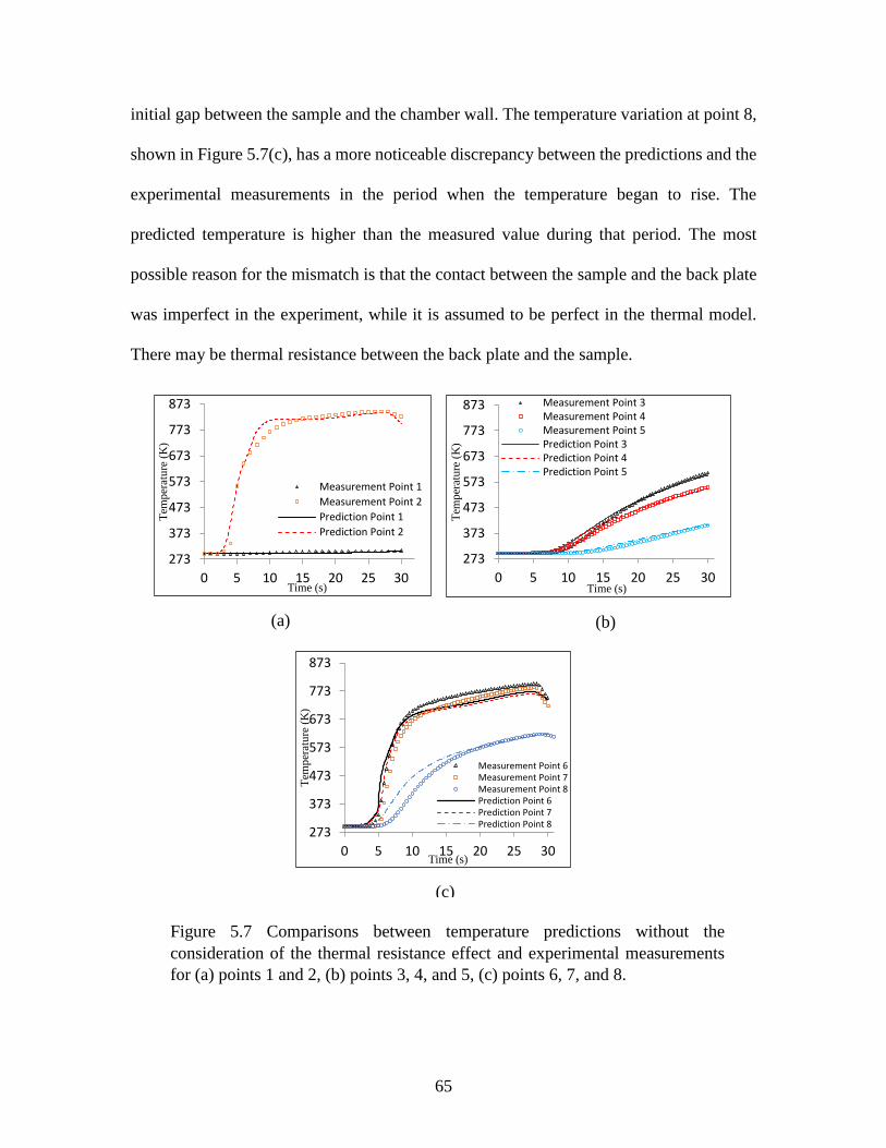
65

initial gap between the sample and the chamber wall. The temperature variation at point 8,

shown in Figure 5.7(c), has a more noticeable discrepancy between the predictions and the

experimental measurements in the period when the temperature began to rise. The

predicted temperature is higher than the measured value during that period. The most

possible reason for the mismatch is that the contact between the sample and the back plate

was imperfect in the experiment, while it is assumed to be perfect in the thermal model.

There may be thermal resistance between the back plate and the sample.

(a)

273

373

473

573

673

773

873

0 5 10 15 20 25 30

Tem

per

atu

re (

K)

Time (s)

Measurement Point 1

Measurement Point 2

Prediction Point 1

Prediction Point 2

(b)

273

373

473

573

673

773

873

0 5 10 15 20 25 30

Tem

per

atu

re (

K)

Time (s)

Measurement Point 3Measurement Point 4Measurement Point 5Prediction Point 3Prediction Point 4Prediction Point 5

Figure 5.7 Comparisons between temperature predictions without the

consideration of the thermal resistance effect and experimental measurements

for (a) points 1 and 2, (b) points 3, 4, and 5, (c) points 6, 7, and 8.

(c)

273

373

473

573

673

773

873

0 5 10 15 20 25 30

Tem

per

atu

re (

K)

Time (s)

Measurement Point 6Measurement Point 7Measurement Point 8Prediction Point 6Prediction Point 7Prediction Point 8

66

In order to confirm the thermal resistance, a simulation with every setting the same

except changing the conductivity of the back plate has been conducted. Changing the

conductivity of the back plate from a small value to its normal value, from the beginning

to the start of extrusion, is to model the thermal resistance. The predicted temperature

variations are compared with the experimental measurements again, as shown in Figure

5.8. It is seen that a good agreement can be observed for point 8, indicating the thermal

resistance is properly modeled. For other points, the predictions are almost the same as

those in the first simulation.

(a)

273

373

473

573

673

773

873

0 5 10 15 20 25 30

Tem

per

atu

re (

K)

Time (s)

Measurement Point 1

Measurement Point 2

Prediction Point 1

Prediction Point 2

(b)

273

373

473

573

673

773

873

0 5 10 15 20 25 30

Tem

per

atu

re (

K)

Time (s)

Measurement Point 3Measurement Point 4Measurement Point 5Prediction Point 3Prediction Point 4Prediction Point 5

Figure 5.8 Comparisons between temperature predictions with the

consideration of the thermal resistance effect and experimental measurements

for (a) points 1 and 2, (b) points 3, 4, and 5, (c) points 6, 7, and 8.

(c)

273

373

473

573

673

773

873

0 5 10 15 20 25 30

Tem

per

atu

re (

K)

Time (s)

Measurement Point 6Measurement Point 7Measurement Point 8Prediction Point 6Prediction Point 7Prediction Point 8

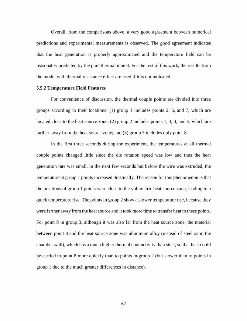
67

Overall, from the comparisons above, a very good agreement between numerical

predictions and experimental measurements is observed. The good agreement indicates

that the heat generation is properly approximated and the temperature field can be

reasonably predicted by the pure thermal model. For the rest of this work, the results from

the model with thermal resistance effect are used if it is not indicated.

5.5.2 Temperature Field Features

For convenience of discussion, the thermal couple points are divided into three

groups according to their locations: (1) group 1 includes points 2, 6, and 7, which are

located close to the heat source zone; (2) group 2 includes points 1, 3, 4, and 5, which are

farther away from the heat source zone; and (3) group 3 includes only point 8.

In the first three seconds during the experiment, the temperatures at all thermal

couple points changed little since the die rotation speed was low and thus the heat

generation rate was small. In the next few seconds but before the wire was extruded, the

temperature at group 1 points increased drastically. The reason for this phenomenon is that

the positions of group 1 points were close to the volumetric heat source zone, leading to a

quick temperature rise. The points in group 2 show a slower temperature rise, because they

were farther away from the heat source and it took more time to transfer heat to these points.

For point 8 in group 3, although it was also far from the heat source zone, the material

between point 8 and the heat source zone was aluminum alloy (instead of steel as in the

chamber wall), which has a much higher thermal conductivity than steel, so that heat could

be carried to point 8 more quickly than to points in group 2 (but slower than to points in

group 1 due to the much greater differences in distance).

68

After 10 seconds, the temperature continued to increase but still in different ways

at points in different groups. In group 1 the temperature obviously increases slowly. At the

end of extrusion, the temperature at point 2 was very near but never attained the solidus

temperature of aluminum alloy 6061, which is physically reasonable. As the temperature

increased gradually after the extrusion of wire started, the aluminum alloy became softer

near the rotating interface and thus was easier to be extruded out to form a wire. Also, the

level of both the friction between the extrusion die and the aluminum alloy and the plastic

deformation decreased since the aluminum alloy became softer due to temperature rise. As

a result, the total heat generation decreased correspondingly, as shown in Figure 5.9. Heat

was conducted away from the heat source zone continually and at the same time the

temperature in group 2 increased almost linearly.

At the end of the extrusion when the die lost contact with the aluminum alloy, the

temperature at point 2 began to drop immediately. The loss of contact resulted in decreased

heat generation and loss of heat transfer to point 2. At points 6 and 7, because the

Figure 5.9 Mechanical power in the experiment.

0

1

2

3

4

5

6

7

8

0 5 10 15 20 25 30

Tota

l h

eat

gen

erat

ion

(kW

)

Time (s)

69

temperature was lower than that in the heat source zone and thus there was still heat transfer

from the heat source zone to points 6 and 7, the temperature here did not decrease

immediately after the end of extrusion but it did decrease later, as shown in Figure 5.8(c).

Similarly at other points, the temperature continued to rise because heat was still being

transferred from high temperature regions to these points.

Figure 5.10 presents the contour graphs of the temperature field on the entire cross

section of the thermal system (they were created by mirroring the model predictions from

one half of the cross section to the other half) at several instants in the friction extrusion

(a) (b)

(c) (d)

Figure 5.10 Predicted temperature contours at (a) t = 7s, (b) t = 14s, (c) t =

21s, (d) t = 27.7s.

Color map (K)

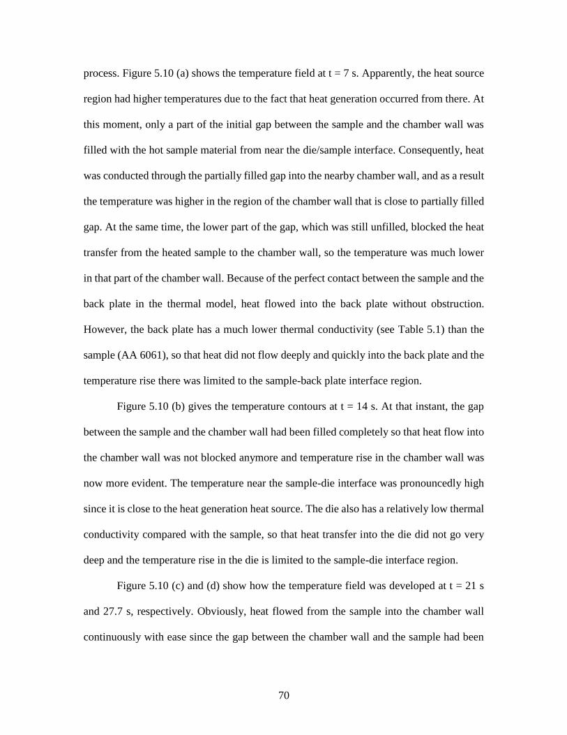
70

process. Figure 5.10 (a) shows the temperature field at t = 7 s. Apparently, the heat source

region had higher temperatures due to the fact that heat generation occurred from there. At

this moment, only a part of the initial gap between the sample and the chamber wall was

filled with the hot sample material from near the die/sample interface. Consequently, heat

was conducted through the partially filled gap into the nearby chamber wall, and as a result

the temperature was higher in the region of the chamber wall that is close to partially filled

gap. At the same time, the lower part of the gap, which was still unfilled, blocked the heat

transfer from the heated sample to the chamber wall, so the temperature was much lower

in that part of the chamber wall. Because of the perfect contact between the sample and the

back plate in the thermal model, heat flowed into the back plate without obstruction.

However, the back plate has a much lower thermal conductivity (see Table 5.1) than the

sample (AA 6061), so that heat did not flow deeply and quickly into the back plate and the

temperature rise there was limited to the sample-back plate interface region.

Figure 5.10 (b) gives the temperature contours at t = 14 s. At that instant, the gap

between the sample and the chamber wall had been filled completely so that heat flow into

the chamber wall was not blocked anymore and temperature rise in the chamber wall was

now more evident. The temperature near the sample-die interface was pronouncedly high

since it is close to the heat generation heat source. The die also has a relatively low thermal

conductivity compared with the sample, so that heat transfer into the die did not go very

deep and the temperature rise in the die is limited to the sample-die interface region.

Figure 5.10 (c) and (d) show how the temperature field was developed at t = 21 s

and 27.7 s, respectively. Obviously, heat flowed from the sample into the chamber wall

continuously with ease since the gap between the chamber wall and the sample had been

71

completely filled. Correspondingly, the temperature in the chamber wall rose continuously.

The region below the die/sample interface always had the highest temperatures and the

material in this region was the source of the subsequently extruded wire. It is also clearly

shown that heat flowed into the die slowly.

From the model predictions, it can be seen that the highest temperature is about 848

K, which occurred at the end of the extrusion and at a location within the heat generation

zone. This highest temperature was below the aluminum alloy’s solidus temperature of 855

K, so that melting did not occur. It is consistent with experiment observation that there is

no defects or voids in the remnant sample that indicate melting.

5.6 Predicted Highest Temperature Variation

The highest temperature that the extruded wire experiences is of great interest since

it is expected to play an important role in determining the mechanical properties of the

extruded wire. Figure 5.11 depicts the predicted highest temperature variation near the

extrusion hole. The predictions show that the temperature at the extrusion hole increases

Figure 5.11 The predicted highest

temperature variation near the hole.

273323373423473523573623673723773823873

0 5 10 15 20 25 30

Tem

per

atu

re (

K)

Time (s)

72

rapidly and then changes little after the start of wire extrusion, which is very similar to the

temperature measured experimentally at point 2. After the start of wire extrusion the

temperature at the extrusion hole varies from 833 K to 848 K. At the end of the extrusion,

the temperature at the hole is 848 K, which is very close to the solidus temperature of 855

K.

5.7 Summary and Conclusions

A pure thermal model has been developed to study the heat transfer phenomenon

during friction extrusion process in this chapter. The heat generation in friction extrusion

process is approximated by a volume heating model. A material layer under the die-sample

interface is chosen as a heat source zone. The total power input is related to the mechanical

power in the experiment. Only heat transfer is simulated and no material flow is considered.

All bodies involved in the experiment are modeled in the simulation and some of them

have smaller geometry sizes. The gap between the sample and the die is modeled by

changing material conductivity.

The temperature predictions from the thermal model agree well with the

experimental measurements, thus providing a good validation of the proposed thermal

model. From the results of this study, it can be concluded as follows

1. The volume heating method can be used to reasonably represent the heat source in

the friction extrusion process.

2. The initial gap between the sample and the chamber wall needs to be modeled in

order to properly capture the heat transfer phenomenon.

73

3. The thermal contact between the billet charge sample and the back plate is not

perfect based on comparisons between predictions and experimental measurements,

and its complication needs to be studied further.

4. The extruded wire experienced a small range of temperature history during

extrusion that varied in a small range somewhat below the solidus temperature.

74

CHAPTER 6 THERMO-FLUID MODELING OF THE FRICTION

EXTRUSION PROCESS

So far, the friction extrusion process has received little attention and development

since it was invented until recently. Tang and Reynolds [3] were the first researchers who

published studies about friction extrusion process. In their work, they conducted a series

of experiments with aluminum alloy chips at several die rotation rates. They tested the

extruded wires on several aspects, such as microstructure, hardness and bend ductility.

They concluded that defect free and good quality wires can be directly produced by friction

extrusion process and limits on the process is related to extrusion temperature. Zhang et al.

[129] studied the friction extrusion process on material flow. At first, a simplified model

without extrusion was analyzed through analytical solution, numerical simulation and

experiments with transparent fluid as presented in Chapter 4. Next a numerical modeling

was conducted to study the material flow features. Since no experimental data was

available for temperature field at that time, only flow fields were discussed. Zhao et al.

[130] performed a physical modeling of friction extrusion process using a transparent fluid

and digital image correlation to track the motion of tiny solid particles in the fluid. Zhang

et al. [131] investigated the heat transfer phenomenon in friction extrusion process by a

pure thermal model as reported in Chapter 5. A volume heating model was proposed to

approximate the heat generation during friction extrusion. It was assumed temperature field

is affected little by material flow field so the flow field was not considered. The temperature

predictions have a very good agreement with experimental measurements. Experimental

75

studies were presented by Li et al. [132, 133] on friction extrusion process with aluminum

alloys. A marker insert technique was used to obtain the material deformation and

distribution. However, information about the distribution of marker material in the chamber

could hardly be obtained due to invisibility.

The previous studies pertaining to friction extrusion process, either focusing on

material flow but without validated temperature field [129], or concentrating on heat

transfer without consideration of material flow [131], or presenting experimental

measurements and observations only [3, 132, 133], none of them provide an understanding

from a comprehensive model that considers both heat transfer and material flow both of

which are involved in friction extrusion process. That also leaves a bunch of questions

waiting answers, such as (1) will the volume heating model still work if material flow field

is considered? (2) what is the material flow field like if validated temperature filed is

applied? (3) how the marker material is distributed in the process chamber during the

process? and (4) how the material deforms before it is extruded out to form a wire? To

answer these questions, a more comprehensive model that includes more details and less

simplifications and assumptions is needed.

The objective of this chapter is to develop such a more comprehensive numerical

model of friction extrusion process that combines both heat transfer and material flow

which exist simultaneously in the process. The relation between temperature field and

material flow field during friction extrusion process is complicated. As other processes

involving large deformations, like friction stir welding and traditional extrusion process,

heat generation comes from both viscous dissipation and friction between workpiece and

tools [97, 125, 134]. Before the temperature gets high, little plastic deformation happens

76

and the heat generation mainly comes from friction. The metal becomes softened when

temperature is high due to continued frictional heating and plastic deformation or material

flow occurs easily. As long as a part of material sticks to the rotating die, the frictional

heating decreases and plastic dissipation increases. The sticking and high temperature

result a zone where the material has prominent velocity. As is seen, the temperature field

and material flow field are coupled because they affect each other. Ideally, the two

phenomena should not be decoupled in numerical simulations. However, at current stage,

it is very hard to implement heat transfer and material flow coupling due to some

difficulties, such as inaccurate material constitutive models at high temperature and strain

rates and some uncertainties about boundary conditions. A better choice is to adopt a

thermal model that is an approximation of the heat generation during the process based on

analytical solutions combined with some reasonable assumptions. In the study of friction

stir welding which shares a lot of similarities with friction extrusion process, it is popular

to use pure thermal models to study the heat transfer [87, 90, 92] and to adopt the thermal

models in material flow modeling [94, 105, 106, 113, 114, 123]. Good agreements with

experimental measurements can be observed for these models. This method is also chosen

in the current work and the thermal model in the heat transfer modeling in Chapter 5 is

adopted. However, the temperature field will not be the same because the material flow

affects heat transfer more or less. The material flow can be modeled in either a solid way

or a fluid way. In order to avoid the difficulties caused by large material deformations, the

current work uses the CFD method so it is a thermo-fluid model.

77

6.1 Governing Equations

Since this is a thermo-fluid model, both temperature and velocity fields need to be

solved although they are not coupled. For the velocity field, the same continuity equations

in Chapter 4 are used and they are given below for completeness.

𝜕𝑣𝑖

∂𝑥𝑖= 0 (6.1)

The Navier-Stokes equations, which are derived from Newton’s second law of motion in

form of momentum, for transient incompressible fluid flow are written as

𝜌𝜕𝑣𝑗

𝜕𝑡+ 𝜌𝑣𝑖

𝜕𝑣𝑗

𝜕𝑥𝑖= −

𝜕𝑃

𝜕𝑥𝑗+

𝜕

𝜕𝑥𝑖(𝜇

𝜕𝑣𝑗

𝜕𝑥𝑖) + 𝐹𝑗 (6.2)

where 𝑣𝑖 are velocity component and 𝐹𝑖 are body force components.

Since there is material flow, the governing equations are a little different from these

for the pure thermal model. The material flow causes heat convection in the fluid. The

conservation of energy can be expressed by

𝜌𝑐𝑝 (𝜕𝑇

𝜕𝑡+ 𝑣𝑖

𝜕𝑇

𝜕𝑥𝑖) =

𝜕

𝜕𝑥𝑖(𝑘

𝜕𝑇

𝜕𝑥𝑖) + Ψ + 𝑞 (6.3)

where 𝑞 is heat generation rate per volume and Ψ is the viscous dissipation due to material

flow, a heat generation source. The viscous dissipation function is expressed as follows

Ψ = 𝜇 [2 (𝜕𝑣1

𝜕𝑥1)

2

+ 2 (𝜕𝑣2

𝜕𝑥2)

2

+ 2 (𝜕𝑣3

𝜕𝑥3)

2

+ (𝜕𝑣1

𝜕𝑥2+

𝜕𝑣2

𝜕𝑥1)

2

+ (𝜕𝑣3

𝜕𝑥2+

𝜕𝑣2

𝜕𝑥3)

2

+ (𝜕𝑣1

𝜕𝑥3+

𝜕𝑣3

𝜕𝑥1)

2

]

(6.4)

From the above equation, it is seen that the viscous heating is directly related with velocity

gradients. In friction extrusion process, large velocity gradients happen near the die/sample

interface. Thus it is expected that a large proportion of heat generation comes from the

vicinity of the interface where strong material flow occurs.

78

6.2 Constitutive Models

The most familiar aspect of a fluid’s properties for us is it can flow with shape

changing. Some fluids are easy to flow and some don’t. The difference is related to a fluid

property called the viscosity, which was first described by Newton. Take an example to

explain the viscosity. Consider two parallel plates filled with a fluid between them. Set one

plate in motion with respect to the other at a low constant velocity. The force per unit area

to keep the motion of the plate is

𝐹

𝐴= 𝜏 = 𝜇

𝑉

∆𝐿= 𝜇휀̇ (6.5)

where 𝜏 is the shear stress in the direction of motion on a fluid surface at a distance ∆𝐿

from the moving plate, 𝜇 is a proportionality, called the viscosity, and 휀̇ is the strain rate

or rate of shear in the fluid. For some fluids, such as water and other pure liquids, the

viscosity doesn’t depend on the strain rate and they are called Newtonian fluids. But some

fluids, such as suspensions of solids in liquid and softened metals, are not Newtonian fluids.

However, equation (6.5) is still used to characterize their properties with the viscosity as a

function of the strain rate. They are called non-Newtonian fluids.

To solve the governing equations, the most important thing is to define the

constitutive equations for the materials. For fluid-based modeling, the Eulerian description

of motion is used, meaning the material particles go through mesh grids which are fixed in

the space. The field variables include velocity and pressure. The viscosity appears in the

Navier-Stokes equations so the constitutive equation needed is for the viscosity. It is

important to point out that the strain is not available directly in fluid modeling and

difficulties emerge if the viscosity is strain dependent. Many researchers have studied the

constitutive equations by proposed mathematical models through experimental tests. There

79

are numbers of different types of mathematical models even for a same material. Suitable

constitutive models should be chosen based one the problem to be solved. The following

sub-sections will focus on the constitutive models chosen for the numerical simulations in

this work.

For a fluid, beside the material properties like density, thermal conductivity, and

specific heat, viscosity is indispensable during numerical modeling of flow. For a regular

fluid, the viscosity can be measured directly through experiments. But for a solid, usually

there is no way to measure it directly. In general, the constitutive equation of a solid is the

stress-strain curve obtained from uniaxial tension test. For some aluminum alloys, such as

AA6061, show visco-platic characteristics, which are rate-dependent inelastic behavior of

solids, and the flow stress is dependent on temperature and strain rates under large

deformations. The material flow is in a viscous manner when large deformations occur

under visco-plastic conditions and the elastic deformations are negligible compared with

total deformations. For a solid under large deformations, correlating the flow stress with

the viscosity is one way to simulate the flow of the material.

For a viscous, incompressible fluid, the constitutive relation can be written in the

form with index notation (i, j, and k represent x, y, and z coordinates, respectively in three-

dimensional Cartesian coordinate system) as follows

𝜎𝑖𝑗 = −𝑃𝛿𝑖𝑗 + 2𝜇휀�̇�𝑗 (6.6)

where 𝜎𝑖𝑗 are stresses, 𝑃 = −𝜎𝑖𝑖/3 is the mean stress, and 휀�̇�𝑗 are the strain rate

components. From equation (6.6), the strain rates can be written as

휀�̇�𝑗 =1

2𝜇𝑠𝑖𝑗 (6.7)

where 𝑠𝑖𝑗 are deviatoric stress components.

80

For a solid behaving visco-plastic characteristics under large deformation, the

constitutive relation can be written [46]

휀�̇�𝑗 =1

�̅�< 𝐹 >

𝜕𝐹

𝜕𝜎𝑖𝑗 (6.8)

where �̅� is a constant ‘pseudo-viscosity’, 𝐹 = 𝐹(𝜎𝑖𝑗) is a yield function. When 𝐹 = 0 it is

plastic yield condition. < 𝐹 >= 𝐹 if 𝐹 > 0 and < 𝐹 >= 0 if 𝐹 ≤ 0. If the von Mises

criterion is chosen, the yield function becomes

𝐹 = √1

2𝑆𝑖𝑗𝑆𝑖𝑗 −

1

√3𝜎𝑒 (6.9)

where 𝜎𝑒 is the flow stress obtained from uniaxial test. Then

𝜕𝐹

𝜕𝜎𝑖𝑗=

1

2

1

√1

2𝑆𝑖𝑗𝑆𝑖𝑗

𝑆𝑖𝑗 (6.10)

If plastic deformations occur, namely 𝐹 > 0, impose equations (6.9) and (6.10) into (6.8)

and use (6.7), we can get

1

𝜇=

1

�̅�

√1

2𝑆𝑖𝑗𝑆𝑖𝑗−

1

√3𝜎𝑒

√1

2𝑆𝑖𝑗𝑆𝑖𝑗

(6.11)

From equation (6.7),

√1

2𝑆𝑖𝑗𝑆𝑖𝑗 = 𝜇√3√

2

3휀�̇�𝑗휀�̇�𝑗 = √3𝜇휀̅̇ (6.12)

where 휀̅̇ is an effective strain rate and its expressed by

휀�̇�𝑗 =1

2(

𝜕𝑣𝑖

𝜕𝑥𝑗+

𝜕𝑣𝑗

𝜕𝑥𝑖) (6.13)

where 𝑣𝑖 are velocity components. Inserting equation (6.12) into (6.11) and changing the

form, an equivalent viscosity is finally obtained

𝜇 =3�̅��̇̅�+𝜎𝑒

3�̇̅� (6.14)

81

For ideal plastic flow, �̅� tends to infinity and (6.14) becomes

𝜇 =𝜎𝑒

3�̇̅� (6.15)

Since the viscosity is strain rate dependent, it is non-Newtonian. The flow stress is

correlated with the viscosity and the expression of the viscosity can be obtained after

knowing the flow stress.

In a large range of temperature and strain rate, for most metals, the effects of

temperature and strain rate to flow stress are not negligible and they must be considered in

the design and control of manufacturing processes. Many researchers have studied the

temperature and strain rate dependent properties of several materials. Due to numerous

challenges encountered in measuring mechanical properties at high temperature and high

strain rates, the data base of experimental measurements is limited. Consequently, the best

option is to propose trusted constitutive models to do some reasonable extrapolations.

Mukai et al. [135] tested the influence of strain rate on flow stress of fine-grained IN905XL

aluminum alloys. They concluded that the yield strength for IN905XL is a weak function

of strain rate when the strain rate is below 10 s-1 and is a strong function when it is up to

1×103 s-1. They also observed negative strain rate sensitivity of the flow stress. Malas and

Seetharaman [136] presented a comprehensive methodology for modeling material

behavior during hot-deformation processing. Balasubrahmanyam and Prasad [137]

investigated the mechanisms of hot deformation in the alloy Ti-5.5Al-1Fe in a temperature

range 750 to1150℃ and a strain rate range 0.001 to 100 s-1 by compression tests. Chen et

al. [138] did research on the stress-strain behavior of aluminum alloy 6xxx and 7xxx at a

wide range of strain rates. They concluded that AA6xxx alloys exhibit no significant rate

sensitivity while moderate rate sensitivity for AA7xxx alloys.

82

Zener and Hollomon designed an experiment in 1944 [100] to validate their

proposed equivalence of the effects of changes in strain rate and in temperature upon the

stress-strain relation in metals. They found that the stress-strain relation in steels depends

on strain rate and temperature only through a single parameter, now called Zener-Hollomon

parameter Z,

𝑍 = 휀̅̇ exp (𝑄

𝑅𝑇) = 𝐴[sinh (𝛼𝜎)]𝑛 (6.16)

where Q is the activation energy, R is the universal Gas constant, and T is the absolute

temperature, A, 𝛼, and n are material constants. Many people developed this relation and

made it widely accepted not only on steels but other BCC and FCC crystalline materials.

Later, Sheppard and Wright [99] developed a form of steady state constitutive relationship

that is convenient and only needs the Zener-Hollomon parameter, as expressed below

𝜎 =1

𝛼ln {(

𝑍

𝐴)

1/𝑛

+ [(𝑍

𝐴)

2/𝑛

+ 1]1/2

} (6.17)

It is obvious that in this equation the flow stress is only a function of temperature and strain

rate and the strain effect is neglected.

This constitutive relationship has been widely used in hot working processes, such

as extrusion and rolling, and also was used by aluminum companies for on line control in

extrusion and tandem mill rolling. Sheppard [139] applied this relationship to AA2024 and

established pressure and speed limitations for varying section shapes. Clode and Sheppard

[140] also used this equation to study hot extrusion process and found that pressure

requirements, microstructural features, and surface defects, pickup and die lines can be

characterized through mathematical formulae and represented within a limit diagram

framework. Sheppard and Jackson [141] conducted experiments on a series of aluminum

alloys from the 1XXX to the 7XXX and published the constants of the constitutive

83

relationship. Duan and Sheppard [142] compared the difference of the equation (6.17) and

other two constitutive equations in the application of numerical simulations in hot rolling

process.

Although there are other forms of constitutive relationships for flow stress, such as

the Johnson-Cook model [143], the Zener-Holloman model is chosen for the viscosity in

the current work. One reason is that in the fluid modeling the variables don’t include strain

and the equation (6.17) neglects strain effect. The other one is that it has been widely used

in numerical simulations of hot working of aluminum alloys, such as hot extrusion and

friction stir welding, which are similar processes as friction extrusion process. Also the

equation (6.17) has been studied on aluminum alloys by many researchers and the constants

are verified to be reliable. If the flow stress in equation (6.17) is put into equation (6.15),

the complete of viscosity can be obtained as follows

𝜇 =1

3�̇̅�𝛼ln {(

𝑍

𝐴)

1/𝑛

+ [(𝑍

𝐴)

2/𝑛

+ 1]1/2

} (6.18)

In this form, the viscosity is only a function of temperature and strain rate since the

constitutive equation of flow stress has no strain effect.

If the equation (6.18) is used for viscosity expression, some artificial modifications

should be made to avoid numerical difficulties. Notice that the value of viscosity

approaches infinity when the strain rate tends to zero. In friction extrusion process, there

exists a large area where deformation is small and the strain rate may be close to zero. To

avoid such errors, a minimum value also is set for the strain rate. It is set not smaller than

10-4 s-1. An enough large number, 1012 Pa-s, is also chosen by referring to simulations on

friction stir welding [97]. Beyond this value, the viscosity is set to equal to it.

84

The material constants in equation (6.18) for aluminum alloy 6061 can be found in

the literature [141]. The values for the constants are listed in Table 6.1.

Table 6.1 Parameters for flow stress (from [141])

Metal 𝛼 (MPa-1) 𝑛 𝑄 (J-mol-1) 𝐺 ln 𝐴 (s-1)

AA6061 0.045 3.55 145,000 8.314 19.3

6.3 Model Description

As indicated before, to study the friction extrusion process with the combination of

both heat transfer and material flow field, a three dimensional CFD model has been

developed. The model includes all parts in the experiment, such as the die, the chamber

wall, the back plate, and the table. Only limited parts of the die, back plate, and table are

modeled in the simulation and their sizes used in the model are chosen so that they represent

them well. The other parts have actual geometrical dimensions of the experimental setup.

The finite volume method is used to discretize the computational domain. In the modeling,

the precursor material is treated as a non-Newtonian fluid and the other parts are considered

as rigid solids. A cross section of a converged mesh is shown in Figure 6.1. The minimum

size of the mesh is located at boundary layers which are close to the interfaces between

solids and fluid and its size is 0.05 mm and the maximum cell size is 1.2 mm. The

commercial code ANSYS FLUENT is used for the computation.

As stated above, the heat transfer and material flow are modeled not in a fully

coupled way and the thermal model in Chapter 5 is adopted in the current modeling. It uses

a small layer of the aluminum alloy sample under the interface between the sample and the

rotating die as the heat generation source to approximate the heat generation during the

friction extrusion process. A uniform height of 4 mm for the layer is taken based on

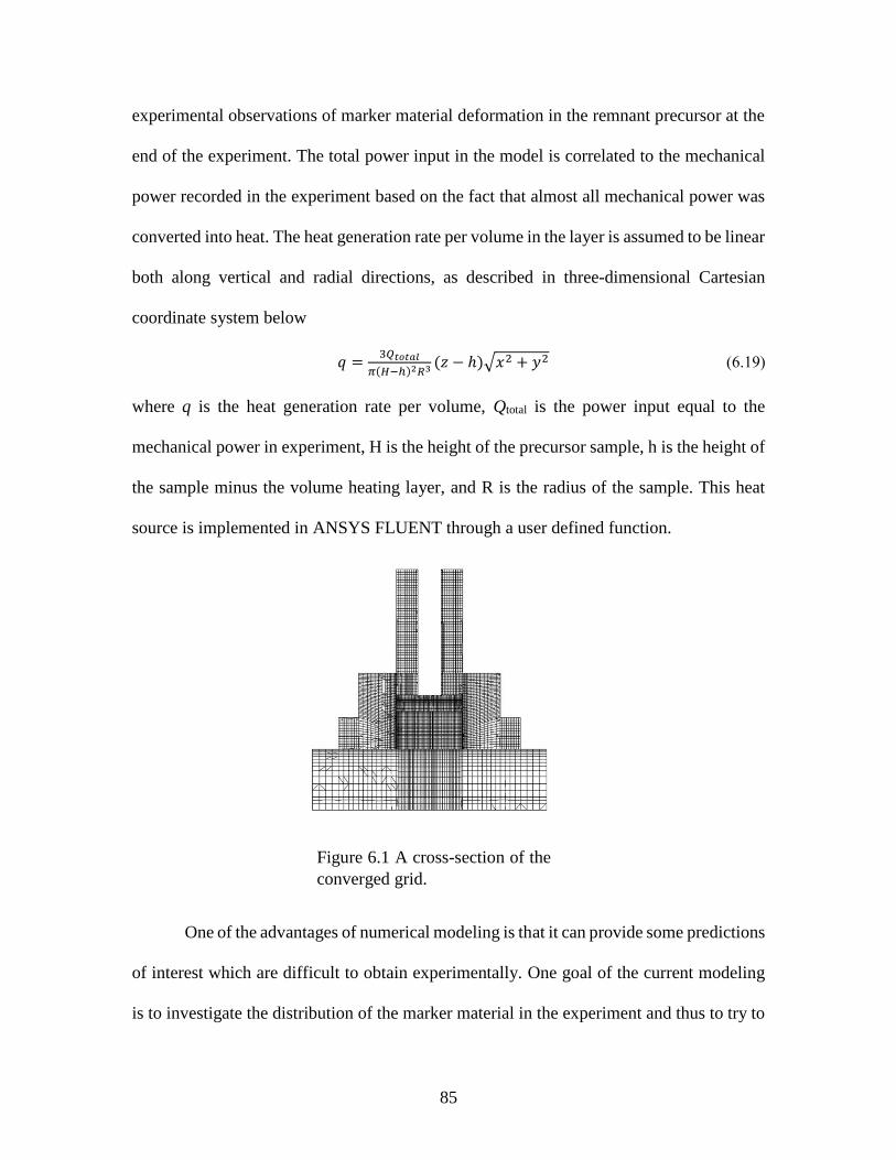
85

experimental observations of marker material deformation in the remnant precursor at the

end of the experiment. The total power input in the model is correlated to the mechanical

power recorded in the experiment based on the fact that almost all mechanical power was

converted into heat. The heat generation rate per volume in the layer is assumed to be linear

both along vertical and radial directions, as described in three-dimensional Cartesian

coordinate system below

𝑞 =3𝑄𝑡𝑜𝑡𝑎𝑙

𝜋(𝐻−ℎ)2𝑅3 (𝑧 − ℎ)√𝑥2 + 𝑦2 (6.19)

where q is the heat generation rate per volume, Qtotal is the power input equal to the

mechanical power in experiment, H is the height of the precursor sample, h is the height of

the sample minus the volume heating layer, and R is the radius of the sample. This heat

source is implemented in ANSYS FLUENT through a user defined function.

One of the advantages of numerical modeling is that it can provide some predictions

of interest which are difficult to obtain experimentally. One goal of the current modeling

is to investigate the distribution of the marker material in the experiment and thus to try to

Figure 6.1 A cross-section of the

converged grid.

86

understand the material flow pattern. However, since the Eulerian description of motion is

used in this simulation, it is very difficult to track the material flow directly. Alternatively,

tracking released solid particles in the fluid can achieve the goal. In this model, several

massless solid particles with a 10-3 mm diameter are used as markers released in the

precursor material which is considered as a fluid in the chamber. The particles are initially

positioned on the ZX plane with different radii. Because these particles are massless they

don’t affect the interested simulation predictions (e.g. velocity and temperature fields).

Followed with nearby fluid, the particles whose trajectories can be tracked represent the

fluid material flow.

In the friction extrusion process experiment, the die moved down besides rotating

to push the precursor material in the chamber out through the extrusion hole so the

extrusion process was carried out. The displacement of the die is shown in Figure 5.4. In

the modeling, the movement of the die is simulated as input. As the die moves down, the

volume of the fluid in the chamber decreases since a part of it is extruded out. The dynamic

meshing technique in FLUENT is used to handle the change of the fluid computational

domain. To keep the boundary layer near the interface between the die and precursor

material and to avoid computation difficulties, the whole fluid computational domain

moves down with the same vertical velocity as the die while the bottom layers of mesh

disappear gradually. Correspondingly, the volume heating zone moves down to keep it on

top of the fluid.

6.4 Initial and Boundary Conditions

The thermal initial and boundary conditions are the same as those used for the pure

thermal model in Chapter 5 because the same friction extrusion process experiment is used.

87

The gap and the thermal resistance are treated in the same way, i.e. changing the

conductivity.

The current model simulates the process of extrusion which is caused by the vertical

motion of the die. The die moves down at a speed obtained from the die positions recorded

during the experiment, as shown in Figure 5.5. As a result, the wire extrusion rate in the

simulation is consistent with the experiment.

For fluid based numerical modeling, the contact behavior between fluids and solids

must be defined. However, the real contact condition between the die and aluminum alloy

in the friction extrusion experiment may vary during the process and it is currently not

known. For the processes which have characteristics similar to friction extrusion, such as

the friction stir welding and extrusion, several researchers have studied the contact

condition between tools and workpieces. Valberg and Malvik [134] showed by

experiments that in extrusion process both sticking and slipping conditions existed on the

die. Doude et al.[144] tried to study the influence of tool shoulder contact conditions on

material flow during friction stir welding. Some numerical modeling work [96, 115, 145]

was to investigate the partial sticking/slipping phenomenon during friction stir welding.

Other people adopted fully sticking condition in CFD modeling of friction stir welding and

obtained reasonable predictions [96, 97, 103]. In the present work, both fully sticking and

partial slipping/sticking conditions are studied.

6.5 Results and Discussions

6.5.1 Thermal Validation

As described in Chapter 2, the temperature at several different positions in the

friction extrusion experiment was recorded. The measured temperature variations with

88

time are compared with numerical predictions as shown in Figure 6.2. In general, a good

agreement between the experimental measurements and the predictions is observed.

For comparisons, the comparisons presented in Chapter 5 between the temperature

predictions in the pure thermal model and the same experimental measurements are shown

in a separate figure Figure 6.3. Since the experimental measurements are the same,

differences of the temperature predictions between the pure thermal model and the thermo-

fluid model can be observed from the comparisons. It is seen that there are unnoticeable

differences for the temperature at point 1, 3, 4, and 5, which are on the outer surfaces, far

from the heat source zone. The temperatures at rest points have mild changes after t = 10

s. The changes come from mainly from the influence of material flow and movement of

the heat generation zone (moving down pushed by the die). The material flow introduces

convection heat transfer in the material and the movement of the heating zone results in

variations of the distances from the heat source to the temperature measurement points.

The temperature at sensitive points (point 2, 6, and 7) which are closer to the heat source

zone have larger changes. For point 8, the difference is very small.

Figure 6.2 Comparisons between temperature predictions of the

thermo-fluid model and experimental measurements.

273

373

473

573

673

773

873

0 5 10 15 20 25 30

Tem

per

ature

(K

)

Time (s)

Measurement Point 1Measurement Point 2Measurement Point 3Measurement Point 4Measurement Point 5Measurement Point 6Measurement Point 7Measurement Point 8Prediction

89

It is shown from the comparisons above that (1) the temperature field can be

reasonably predicted by using the pure thermal model in the current decoupled thermo-

fluid model, (2) thus the method used in friction stir welding, applying thermal models in

fluid modeling, also works in modeling of friction extrusion process, and (3) the material

flow has very limited influence on the heat transfer phenomenon.

6.5.2 Material Flow Validation

Interpolation

As described in section 6.4, some massless solid particles are released in the

precursor material which is a fluid in the modeling. These particles can be tracked and their

trajectory paths can be recorded during the simulation. In the modeling only some of

particles are extruded out of the chamber and the distribution of them on the extruded wire

can be compared with experimental measurements. In the experiment, the traces of the

marker material can be observed clearly on the extruded wire cross sections although it

was distorted and stretched since the marker material is a continuum. However, in the

Figure 6.3 Comparisons between temperature predictions of the

pure thermal model and experimental measurements.

273

373

473

573

673

773

873

0 10 20 30

Tem

per

ature

(K

)

Time (s)

Measurement Point 1Measurement Point 2Measurement Point 3Measurement Point 4Measurement Point 5Measurement Point 6Measurement Point 7Measurement Point 8Prediction

90

simulation, the number of the solid particles is finite and it is not enough to have a better

view effect when comparing them with experimental observations on wire cross sections.

To have better comparisons, interpolations of the predictions about the particles positions

on extruded wire cross sections are necessary to obtain more data points.

Figure 6.4 shows schematics of the initial positions of the marker material in the

experiment and a part of solid particles in the simulation. They are analyzed in a same

cylindrical coordinate system. Interests only focus on the particles which are initially

placed in the same region occupied by the marker material. There are 13 columns of

particles with radius from 2.93 - 5.57 mm and 25 rows with height from 15 - 18 mm on the

z-r plane. In total, there are 325 particles. The region where these particles are placed is

called particle region. The goal is to obtain any data point in the whole marker material

region in the height range of 15 - 18 mm from these particles. Two reasonable assumptions

are made to do the interpolation. First, it is assumed that the radii of the particles to the

center axis keep unchanged after they reach the exit extrusion hole. Second, based on the

axisymmetric geometry, it is assumed that particles, which have the same initial heights,

have same path line shapes in the space. Based on the two assumptions, for any particle in

r

z

𝜃 r

z

𝜃

Figure 6.4 Schematics of (a) aluminum alloy sample

with the marker wire and (b) particles in simulation.

(a) (b)

91

the particle region, the angle and time when it reaches the exit hole can be obtained by

interpolation.

(a) (b) (c)

Figure 6.5 Marker distributions on wire cross sections in experiment at

time (a) t = 13.0 s (b) t = 16.9 s (c) t = 18.8 s.

(a) (b) (c)

Figure 6.6 Predicted marker distributions on wire cross sections with

sticking factor 0.3 at time (a) t = 13.0 s (b) t = 16.9 s (c) t = 18.8 s.

(a) (b) (c)

Figure 6.7 Predicted marker distributions on wire cross sections with

sticking factor 0.6 at time (a) t = 13.0 s (b) t = 16.9 s (c) t = 18.8 s.

92

In the modeling, the positions of the particles at every moment are recorded. For each

particle that is extruded out, the time t and the angle θ when it reaches the exit hole and the

initial coordinates, including radius r and height z, can be obtained. Then two series of data

points with respect to (r, z, θ) and (r, z, t), respectively, are available to do the interpolation.

The objective of the interpolation is to find the time and angle of any particle in the particle

region when it reaches the exit hole based on the available particle data. The interpolation

work is done by my co-worker Mr. Xiao Li. As many as thousands of data points can be

obtained through the interpolation. The time when a particle reaches the exit hole

determines its longitudinal position in the wire since the extrusion rate is known. As a result,

the particles and the marker material on same wire cross sections can be compared.

Comparisons

As mentioned earlier, in this model, different contact conditions have been tried.

Here a sticking factor is defined. A sticking factor indicates the degree of the sticking of

the material to the tool. For example, a sticking factor of 0.3 means the rotating speed of

the fluid on the fluid-solid interface is 30% of the tool rotating speed. In the current

(a) (b) (c)

Figure 6.8 Predicted marker distributions on wire cross sections with

sticking factor 1.0 at time (a) t = 13.0 s (b) t = 16.9 s (c) t = 18.8 s.

93

simulations, 0.3, 0.6, and 1.0 are used to for the sticking factor. Figure 6.5 shows the marker

material distributions during the friction extrusion experiment on extruded wire cross

sections. The marker material shows a dark color after chemical etching. The rest is

aluminum alloy 6061. The predicted marker material distributions on the extruded wire

cross sections with different sticking factor values are shown in Figure 6.6, Figure 6.7, and

Figure 6.8, respectively. From the comparisons of the numerical predictions about the

marker distribution, the marker forms more revolutions of spirals in the simulation with

bigger sticking factor. The can be explained by the fact that the higher sticking factor means

higher rotating speed for the fluid on the fluid-solid interface, resulting in more strong

stirring. However, the experimental observations show the marker material has more

revolutions of spirals on extruded wire cross sections. The predictions with sticking factor

1.0 as shown in Figure 6.8 are closest to the experimental observations, implying that the

sticking factor 1.0 is the best for material flow prediction. Comparing the numerical

predictions and experimental observations, it can be seen that they share some features in

common, such as (a) the markers form continuous spirals on extruded wire cross sections

and (b) the revolutions of the spirals on the cross sections decrease as extrusion continues.

However, some differences exist between the simulation and experimental measurements.

The discrepancies are mainly due to some assumptions made in the modeling. Nevertheless,

the qualitative comparisons indicate that the material flow trends can be captured.

6.5.3 Computed Temperature Field

The predicted temperature fields with different instants are shown Figure 6.9. For

comparisons, the predicted temperature fields in the pure thermal model are also displayed,

as seen in Figure 6.10. It is seen predictions are very similar. The temperature variation

94

trends and magnitude are very close. The features of the temperature fields are not

discussed here since they are discussed in Chapter 5.

(a) (b) (c)

Figure 6.10 Predicted temperature contours at (a) t = 7 s, (b) t =

14 s, (c) t = 21 s.

(g)

Figure 6.11 Predicted velocity contours at (a) t = 10 s, (b) t = 15 s, (c) t = 19 s, (d)

t = 24 s, (e) t = 10 s, (f) t = 15 s, (g) t = 19 s, (h) t = 24 s.

Magnitude Vertical

(a) (b) (c)

(h) (e) (f)

(d)

(a) (b) (c)

Figure 6.9 Predicted temperature contours at (a) t = 7s, (b) t =

14s, (c) t = 21s.

95

6.5.4 Predicted Flow Fields

Figure 6.11 depicts the computed velocity contours on a longitudinal section of the

precursor sample at different instants. Before wire extrusion, as shown in Figure 6.11 (a),

a small region under the die-precursor sample interface has obviously higher velocity. In

the center of the region, the velocity is close to zero due to the lower die rotating speed in

the center. Since there is no die vertical movement or no wire extrusion at this moment,

there is only tangential velocity. The velocity drops drastically when the distance from the

interface increases except near the extrusion hole. The velocity has a peak near the middle

of the radius at same heights. At the corner between the top surface and lateral surface, the

velocity changes from low to high and thus the gradient is high. That’s because the fluid at

the top surface has high tangential velocity near the corner while the velocity is zero on the

lateral surface due to non-slip condition used. The velocity contrast results in such velocity

field in the corner. Figure 6.11 (b) - (d) show resultant velocity fields during wire extrusion

at t = 15 s, 19 s and 24 s, respectively. Compared with Figure 6.11 (a), the contour plots

have no obvious difference except in the region near the extrusion hole. Under the extrusion

hole, there is vertical velocity due to extrusion and the total velocity is noticeable. Since

the extrusion rate is constant, the velocity at this area doesn’t change much. Although that

the temperature in the region beneath the interface between die and the aluminum rises

after the start of wire extrusion as discussed in the last section, the velocity field seems

unchanged. The explanation for this is that the viscosity doesn’t change much in a small

range of temperature and thus the velocity field is little affected. This also can explain that

the wire extrusion rate almost is constant. Figure 6.11 (e) – (h) show the vertical velocity

contours at t = 10 s, 15 s, 19 s and 24 s, respectively. As the resultant velocity contours, the

96

vertical velocity contours at different times after start of wire extrusion look like the same.

A small region around the extrusion hole had relatively higher vertical velocity, indicating

that the vertical velocity is dominant in that area. The predicted velocity fields show that

the stir zone, where the material is experiencing large deformation, keeps almost the same

shape after the start of wire extrusion, since the velocity field doesn’t change much.

Another important flow field variable is strain rate, which reflects the change of

deformation of the material, since it is known that it affects material recrystallization and

can be used to estimate the material microstructure [146]. In other material processes, like

friction stir welding, extrusion and rolling of alloys, researchers tried to establish

relationships between the strain rate and the material grain size or subgrain size. References

[146-148] studied the relationship between grain size and strain rate for AZ31 magnesium

alloy and others [86, 149, 150] investigated the relationships between subgrain size and

strain rate. Due to lack of grain size measurements in this work, the relationship between

grain or subgrain size and strain rate is not discussed and only the predicted strain rate

fields at different times are presented. Figure 6.12 shows the strain rate fields at various

moments after start of extrusion. Only some select contours are shown. The strain rate is

less than 1 /s in the region below the 1 /s contour and it is larger than 100 /s in the area

beyond the 100 /s contour. As the velocity fields, the relative larger strain rates occur in a

small region under the interface between the die and aluminum alloy. In general, the strain

rate fields look like almost the same also as the velocity fields do. The maximum value

area is at the corner between the top surface and lateral surface of the aluminum alloy

sample. That is not different to understand since that the velocity gradient is highest at the

corner can be seen in the velocity fields as shown in Figure 6.11. The iso-valued strain rate

97

contours also converge at the corner. The maximum value of strain rate in the modeling is

larger than 100 /s, which is larger than the values reported in some studies of friction stir

welding [86, 151].

Viscosity is a property that is related to flow stress of the material and that also

determines the fluidity of the material. Computed viscosity field cross sections at different

moments are shown in Figure 6.13. For brief, only some selected value contours are

displayed and only the fluid in chamber is chosen. Since the extrusion of wire results

reduction of the volume of the fluid, the height of the fluid domain decreases with time.

The contours shape is like a bowl with a convex center. Figure 6.13 (a) shows the contours

at time t = 11 s when the extrusion just starts. As seen, the viscosity is lower near the

die/sample interface, especially at the two upper corners and it increases gradually as it is

1

2

20 10 50 100

1

2

20 10 50 100

1

2

20 10 50 100

1

2

20 10 50 100

(a) (b)

(c) (d)

Figure 6.12 Strain rate fields (unit s-1) at (a) t = 11 s (b) t = 16 s (c) t = 20

s (d) t = 24 s.

98

far from the interface vertically. The region below the 1e7 Pa-s contour has larger viscosity.

The features of viscosity distribution can be explained from the temperature fields and

strain rate fields. High temperature softens the material in the chamber so the viscosity is

smaller in higher temperature regions. The temperature in the region near the interface is

higher and the strain rate at the central area is relatively small, together resulting in such

shapes of the viscosity contours. The viscosity contours of the same values at different

moments as shown in Figure 6.13 (a)-(d) indicate that the contours move down slowly.

Nandan et al. [105] reported a cutoff viscosity of 5.0e6 Pa-s (above which no significant

1e10 1e9 1e8

1e7

5e5 5.5e6

1e9 1e8

1e7

5e5 5.5e6

1e10

1e9 1e8

1e7

5e5 5.5e6

1e10 1e9 1e8

1e7

5e5 5.5e6

1e10

(a) (b)

(c) (d)

Figure 6.13 Viscosity fields (unit Pa-s) at time (a) t = 11 s (b) t = 15 s (c) t = 19 s (d)

t = 22 s.

99

material flow occurs) based on experimental observations on AA6061 to find the

characteristic shape of the thermo-mechanically affected zone in a CFD model. The

viscosity contour of this value is also shown in Figure 6.13. It is seen that the thermo-

mechanically affected zone almost keep the same shape and same location relative to the

surface. In general, the viscosity field varies mildly after the start of extrusion.

6.5.5 Material Flow Features

In the modeling, the particle markers released in the precursor material flow with it

and leave continuous trajectory paths. Since the particles are massless, they fallow the

nearby material all the time and thus their trajectory paths represent the nearby material

paths. Studying the paths of particle markers can help understand how the precursor

material in the chamber flows and how the extruded wire is formed. It is worth to note that

numerical modeling is able to provide vivid visualization that is not available in experiment.

Figure 6.14 depicts the path lines of the particle markers with different initial positions in

the simulation. The initial heights of these path lines range from 15 mm to 18 mm. Every

path line has a unique color. For a better view, the figures don’t have the same scale. Figure

6.14 (a) shows a group of path lines which originate from one third of sample radius from

(a)

(b) (c)

Figure 6.14 Path lines with initial positions at (a) r = 4.3 mm (b) r = 7.2 mm (c) r =

10.4 mm from the center.

100

the center. All of these path lines go through the extrusion hole, indicating that the material

there is extruded out of the chamber to form the wire. Before reaching the extrusion hole,

all path lines have experienced spiral shapes which feature decreasing radii and increasing

heights. For those path lines who have higher initial heights, their spirals have more

rotations. The spirals are the consequence of the rotating die which is stuck by the material

at the die-sample interface. Near the interface, material has larger tangential velocity and

thus experiences more rotations. This can explain those path lines with more spirals. The

path lines with lower initial heights have more obvious height increase. The decreasing

radii of spirals show the material flows toward the center and the increasing heights

indicate that the material has vertical velocity. All of these imply that there is material in

the central region being pushed spirally upward the extrusion hole. Figure 6.14 (b) shows

path lines of particles which are released at positions with a distance 7.2mm from the center

(The sample radius is 12.5 mm). Only some of the path lines which have lower initial

positons reach the extrusion hole, meaning that the material in that region with lower

heights flows out of the chamber to compose the extruded wire while those with higher

heights stay in the chamber all the time during the process. The path lines with lower initial

heights show the material there also is pushed to both the center and the extrusion hole

spirally. The spiral shapes of the particles with higher initial heights are different. Since

they stay in the chamber all the time and in the higher velocity region they have experienced

more number of spirals. During the friction extrusion process, the die moves down

gradually, pushing the material just under it down. As a result, the heights of these particles

decrease slowly. Figure 6.14 (c) show the path lines whose initial positions are 10.4 mm

away from the center. Apparently, none of the particles pass the extrusion hole and no

101

material there goes out of the chamber. The number of spirals is obviously less due to the

region has small velocity. Likewise, the radii of the path lines with lower initial heights

decrease but with slight variation. Path lines in Figure 6.14 (b) and (c) show that there

exists a dead zone as in traditional extrusion process where the material can never be

extruded out of the chamber.

6.5.6 Summary and Conclusions

This chapter has presented a three-dimensional thermo-fluid model in order to

provide a comprehensive understanding of the friction extrusion process. Both heat transfer

and material flow are modeled in this model. The volume heat model in Chapter 5 is used

for heat transfer modeling and the thermal resistance between the sample and the back plate

is modeled by changing the conductivity of the back plate. The temperature predictions

have been compared with experimental measurements and the results from the pure thermal

model.

The sample is considered as a non-Newtonian fluid and the CFD method is used to

simulate the material flow. The viscosity of the fluid is a function of strain rate and

temperature. To investigate the material flow pattern and provide data to compare with

experimental measurements, some massless solid particles are used in the fluid to track the

nearby fluid. Different contact conditions between the die and the sample have been tried

and three values are used for the sticking factor.

The comparisons show the temperature predictions have a good agreement with

experimental measurements and the predicted temperature variations are similar with those

in the pure thermal model. The predicted distribution of the particles on extruded wire cross

sections also have the same trends with experimental observations. Some findings are

102

concluded as follows.

1. The material flow has unnoticeable effect on temperature field and the uncoupled

heat transfer and material flow model also works for friction extrusion process.

2. The flow field variables, i.e. velocity, strain rate, and viscosity, almost keep the

same during after the start of extrusion although the temperature field changes all

the time.

3. The particles path lines show that material in the central zone of the process

chamber is pushed spirally towards the extrusion hole to form the extruded wire;

then the material near the central zone moves in to fill the space in the central region;

and material in the upper corner below the die-aluminum alloy interface and away

from the extrusion hole forms the dead zone - the material stays in the chamber and

never get extruded.

103

CHAPTER 7 SUMMARY AND RECOMMENDATION

7.1 Summary

The friction extrusion process has been studied successfully through numerical

simulations in this dissertation. This work includes a flow visualization study by a physical

model with transparent fluid and tools, a pure thermal model that focuses on heat transfer

phenomenon, and a three-dimensional model which takes both heat transfer and material

flow into consideration to provide a comprehensive understanding of the friction extrusion

process.

First, a physical model with a Newtonian fluid was studied to mimic the friction

extrusion process. The flow visualization study is to capture the material feature during

friction extrusion process. It is a simplified model that only has tool rotation and there is

no extrusion part. The model consists of a viscous Newtonian fluid, a chamber wall, and a

back plate. The fluid and the tools are transparent so that experimental observations and

measurements can be achieved easily. The Reynold number is equal to that approximated

in friction extrusion process and it indicates a laminar flow. Due to the regular shapes of

the fluid domain geometry and boundary conditions, an analytical solution about the flow

field can be developed. Some assumptions, such as axisymmetric problem and zero

velocity in radial and vertical directions, were made to enable the analytical solution

attained. A three-dimensional CFD simulation of the simplified model was also performed.

No assumption was made for the numerical modeling. Differences between the analytical

solution and the numerical solution are very small, below 2%. The analytical solution was

104

also compared with experimental measurements implemented by a DIC system on tiny

particles in the fluid. A good agreement can be observed, serving as an evidence for

experimental validation of the analytical solution and CFD simulation predictions.

Next, a pure thermal model was developed to investigate the heat transfer

phenomenon during friction extrusion process. The heat generation approximation is the

crucial when modeling the temperature field. A volume heating model has been proposed

based on the characteristics of the friction extrusion process. The heat generation produced

by friction between the die and aluminum alloy sample and the plastic deformation under

the interface between the die and the sample is represented by a layer under the die-sample

interface. The heat generation rate is assumed linearly distributed along vertical and radial

directions. No frictional heat generation that is in the form of surface flux was included in

the model since it is compensated in the volume heating model. The total power input into

the system is related to the mechanical power during the friction extrusion experiment and

it is assumed all mechanical power is transferred to heat.

The numerical model includes all parts involved in the friction extrusion

experiment, such as the die, the chamber wall, the back plate, the support table, and the

aluminum alloy sample. Only parts of the die, the back plate, and the table are included

and their sizes are chosen to represent these bodies. The material flow is not modeled in

the pure thermal model so all the bodied are treated as solids. As a result, only conduction

equation is needed to solve for the temperature field. The boundary conditions have been

carefully handled. The gap between the die and the aluminum sample is modeled by

changing the conductivity and how it is filled was estimated.

105

The temperature predictions have a good agreement with the experimental

measurements at several points, indicating that the volume heating model can be used to

reasonably represent the heat generation during the friction extrusion process. The

numerical results show the heat transfer phenomenon is a transient process and the

temperature field is changing all the time. However, the temperature under the extrusion

hole doesn’t change much after the start of extrusion. Since the material under the extrusion

hole forms the wire, the thermal history of the extruded wire can be estimated. It’s seen

although it is transient heat transfer, the highest temperature that the wire experiences

changes small. The numerical results also show there is thermal resistance between the

aluminum sample and the back plate.

A three-dimensional thermo-fluid model also has been presented to provide a

comprehensive understanding of the friction extrusion process. Both heat transfer and

material phenomena are modeled and more information can be obtained from the model.

The volume heating model is used for the heat generation source and the assumption made

in the pure thermal model, which is the material flow has small influence to the heat transfer

during friction extrusion process, can be tested in the thermo-fluid model. The thermal

initial and boundary conditions are the same as the pure thermal mode except the contact

between the aluminum alloy sample and the back plate. The thermal resistance is simulated

by changing the conductivity of the back plate. The predicted temperature results show that

the material flow has unnoticeable effect on temperature field and the uncoupled heat

transfer and material flow model works for friction extrusion process.

The Eulerian description of motion is used to simulate the material flow due to

extreme deformation and distortion of the material. The aluminum alloy sample is treated

106

as a non-Newtonian fluid given that the flow stress is strain rate and temperature dependent.

The Zener-Holloman parameter is adopted to describe the constitutive equation. Thus the

fluid viscosity is a function of strain rat and temperature. The tools are seemed as rigid

solids. The geometry sizes of the bodies are same as those in the pure thermal model. For

the contact condition between the rotating die and the aluminum alloy sample which is

treated as a fluid, different values, i.e. 0.3, 0.6, and 1.0, have been tried for the sticking

factor. Massless solid particles are released in the fluid in the simulation as tracers to track

the material flow paths. Since the particles don’t affect the temperature and fluid fields,

they can represent the material flow. The distribution of the particles on the extruded wire

cross sections was compared with experimental measurements. The qualitative

comparisons show that the distribution trends and features can be captured by the thermo-

fluid model. The numerical model provides information that is not available in experiment,

such as the velocity, viscosity, and strain rate fields. The predicted flow fields almost keep

the same after the start of extrusion although the temperature field changes. The path lines

of the particles show that the material in the central zone of the process chamber is pushed

spirally towards to extrusion hole to form the wire; then the material near the central zone

moves to fill the space in the central region; and there is a dead zone in the upper corner

where the material stays in the chamber.

7.2 Recommendations

The current studies about the friction extrusion process have successfully

established numerical models which are able to capture the characteristics of the heat

transfer and material flow phenomena. The numerical simulations are aimed to understand

the mechanisms occurred during the friction extrusion process and to help optimize the

107

experimental designs. Currently, there exists little literature for the friction extrusion

process and the present work is only a first step to studying the friction extrusion process.

There are several open questions and further studies are needed to develop the friction

extrusion process.

One recommendation for further studies is to figure out if the friction extrusion

process can reach steady state and when it reaches steady state. In this work, the experiment

process was not long enough due to equipment restrictions so it was transient. Even though

the temperature field is transient, the simulations show the flow fields don’t change much.

If the process operation is long enough, theoretically it will become steady state.

The current study only focused on one combination of the experimental parameters,

namely the die rotating speed and the pushing force applied on the die, which can produce

good quality wires. Parametric studies using the numerical models reported in this

dissertation are recommended. Parametric studies can find out how the parameters

influences the temperature field and flow field. This is very helpful for the experimental

designs.

Different die shapes may be tried. In this work, the surface of the die that contacts

the aluminum alloy sample is flat. The thermo-fluid model can be used to simulate the

processes with other die surfaces, such scrolled shape. A dead zone was observed in the

simulations and a cone-shaped surface may avoid the dead zone and improve the extrusion

efficiency.

Only the CFD model was used in this dissertation to simulate the friction extrusion

process. The advantage of this model is that the extreme deformation and distortion can be

easily handled. However, the disadvantage is that the contact condition between the die

108

and the aluminum alloy sample must be defined. The contact condition is an important

issue to study the friction extrusion process since it affects the stirring largely. It may be

calculated by a finite element based model. The ALE finite element formulation is a good

choice to deal with the mesh deformation and distortion.

Since the extruded wire is very long relative the sample and the ALE mesh always

keeps its original topology, the wire is not recommended to be included in the ALE

simulation of friction extrusion process. Eulerian surface can be used for the extrusion hole

as an outlet. Because the material in the chamber keeps regular shape, the distortion of

mesh can be easily taken care by the ALE technique. For the friction between the die and

the aluminum alloy sample, the modified Coulomb’s law can be employed. The Zener-

Holloman constitutive equation for the aluminum alloys has been widely used in the

numerical simulations for processes involved large strain rate and high temperature. If this

constitutive equation is used in ALE modeling, a user subroutine may be needed for it.

109

REFERENCES

1. Thomas, W.M., E.D. Nicholas, and S.B. Jones, US Patent # 5,262,123. 1993.

2. http://www.uspto.gov/web/offices/com/sol/og/2002/week04/patexpi.htm.

3. Tang, W. and A.P. Reynolds, Production of wire via friction extrusion of aluminum

alloy machining chips. Journal of Materials Processing Technology, 2010. 210(15):

p. 2231-7.

4. Gronostajski, J. and A. Matuszak, Recycling of metals by plastic deformation: an

example of recycling of aluminium and its alloys chips. Journal of Materials

Processing Technology, 1999. 92-93: p. 35-41.

5. Ding, J., Thermo-mechanical analysis of wire and arc additive manufacturing

process. 2012, Cranfield University: U.K.

6. http://www.nasa.gov/topics/technology/features/ebf3.html.

7. Lange, K. and K. Pöhlandt, Handbook of metal forming. 1985: McGraw-Hill.

8. Malvern, L.E., Introduction to the Mechanics of a Continuous Medium. 1969:

Prentice-Hall.

9. Dieter, G.E., H.A. Kuhn, and S.L. Semiatin, Handbook of Workability and Process

Design. 2003: A S M International.

10. Hibbitt, H.D., P.V. Marcal, and J.R. Rice, A finite element formulation for

problems of large strain and large displacement. International Journal of Solids and

Structures, 1970. 6(8): p. 1069-1086.

11. McMeeking, R.M. and J.R. Rice, Finite-element formulations for problems of large

elastic-plastic deformation. International Journal of Solids and Structures, 1975.

11(5): p. 601-16.

12. Belytschko, T., W.K. Liu, and B. Moran, Nonlinear finite elements for continua

and structures. 2000: Wiley.

13. Bathe, K.J., E.L. Wilson, and E. Ramm, Finite element formulations for large

deformation dynamic analysis. International Journal for Numerical Methods in

Engineering, 1975. 9(2): p. 353-86.

110

14. Wifi, A.S., An incremental complete solution of the stretch-forming and deep-

drawing of a circular blank using a hemispherical punch. International Journal of

Mechanical Sciences, 1976. 18(1): p. 23-31.

15. Lee, E.H., R.L. Mallett, and W.H. Yang, Stress and deformation analysis of the

metal extrusion process. Computer Methods in Applied Mechanics and

Engineering, 1977. 10(3): p. 339-53.

16. Odell, E.I., A Study of Wall Ironing by the Finite Element Technique. Journal of

Engineering for Industry, 1978. 100(1): p. 31-36.

17. Wang, N.M. and B. Budiansky, Analysis of sheet metal stamping by a finite-

element method. Transactions of the ASME. Journal of Applied Mechanics, 1978.

45(1): p. 73-82.

18. Gotoh, M., A finite element analysis of general deformation of sheet metals.

International Journal for Numerical Methods in Engineering, 1974. 8(4): p. 731-

741.

19. Oh, S.I. and S. Kobayashi, Finite element analysis of plane-strain sheet bending.

International Journal of Mechanical Sciences, 1980. 22(9): p. 583-594.

20. Wifi, A.S., Finite element correction matrices in metal forming analysis (with

application to hydrostatic bulging of a circular sheet). International Journal of

Mechanical Sciences, 1982. 24(7): p. 393-406.

21. Yamada, Y., A. Wifi, and T. Hirakawa. Analysis of large deformation and stress in

metal forming processes by the finite element method. in Metal Forming Plasticity\

Proc. Conf.\, Tutzing, Germany, Aug.-Sept. 1978. 1979.

22. Nagtegaal, J.C. and J.E. De Jong, Some computational aspects of elastic-plastic

large strain analysis. International Journal for Numerical Methods in Engineering,

1981. 17(1): p. 15-41.

23. Kudo, H. and S. Matsubara, JOINT EXAMINATION PROJECT OF VALIDITY

OF VARIOUS NUMERICAL METHODS FOR THE ANALYSIS OF METAL

FORMING PROCESSES. NASA Conference Publication, 1979: p. 378-403.

24. Rao, S.S. and A. Kumar, Finite element analysis of cold strip rolling. International

Journal of Machine Tool Design and Research, 1977. 17(3): p. 159-168.

25. Argyris, J.H. and J.S. Doltsinis, On the large strain inelastic analysis in natural

formulation part I: Quasistatic problems. Computer Methods in Applied Mechanics

and Engineering, 1979. 20(2): p. 213-251.

26. Argyris, J.H. and J.S. Doltsinis, On the large strain inelastic analysis in natural

formulation part II. Dynamic problems. Computer Methods in Applied Mechanics

and Engineering, 1980. 21(1): p. 91-126.

111

27. Nagtegaal, J.C. and N. Rebelo, On the development of a general purpose finite

element program for analysis of forming processes. International Journal for

Numerical Methods in Engineering, 1988. 25(1): p. 113-131.

28. Strenkowski, J.S. and K.-J. Moon, Finite Element Prediction of Chip Geometry and

Tool/Workpiece Temperature Distributions in Orthogonal Metal Cutting. Journal

of Engineering for Industry, 1990. 112(4): p. 313-318.

29. Voyiadjis, G.Z. and M. Foroozesh, A finite strain, total Lagrangian finite element

solution for metal extrusion problems. Computer Methods in Applied Mechanics

and Engineering, 1991. 86(3): p. 337-70.

30. Jung-Ho, C. and K. Noboru, An analysis of metal forming processes using large

deformation elastic-plastic formulations. Computer Methods in Applied Mechanics

and Engineering, 1985. 49(1): p. 71-108.

31. Kobayashi, S., A review on the finite-element method and metal forming process

modeling. Journal of Applied Metalworking, 1982. 2(3): p. 163-169.

32. Lee, C.H. and S. Kobayashi, New Solutions to Rigid-Plastic Deformation Problems

Using a Matrix Method. Journal of Engineering for Industry, 1973. 95(3): p. 865-

873.

33. Zienkiewicz, O.C. and P.N. Godbole, A penalty function approach to problems of

plastic flow of metals with large surface deformations. Journal of Strain Analysis,

1975. 10(3): p. 180-3.

34. Lung, M. and O. Mahrenholtz, FINITE ELEMENT PROCEDURE FOR

ANALYSIS OF METAL FORMING PROCESSES. Transactions of the Canadian

Society for Mechanical Engineering, 1973. 2(1): p. 31-36.

35. Kobayashi, S., RIGID-PLASTIC FINITE ELEMENT ANALYSIS OF

AXISYMMETRIC METAL FORMING PROCESSES. 1977: p. 49-65.

36. Chen, C.C. and S. Kobayashi, RIGID PLASTIC FINITE ELEMENT ANALYSIS

OF RING COMPRESSION. American Society of Mechanical Engineers, Applied

Mechanics Division, AMD, 1978. 28: p. 163-174.

37. Gotoh, M. and F. Ishisé, A finite element analysis of rigid-plastic deformation of

the flange in a deep-drawing process based on a fourth-degree yield function.

International Journal of Mechanical Sciences, 1978. 20(7): p. 423-435.

38. Gotoh, M., A finite element analysis of the rigid-plastic deformation of the flange

in a deep-drawing process based on a fourth-degree yield function—II.

International Journal of Mechanical Sciences, 1980. 22(6): p. 367-377.

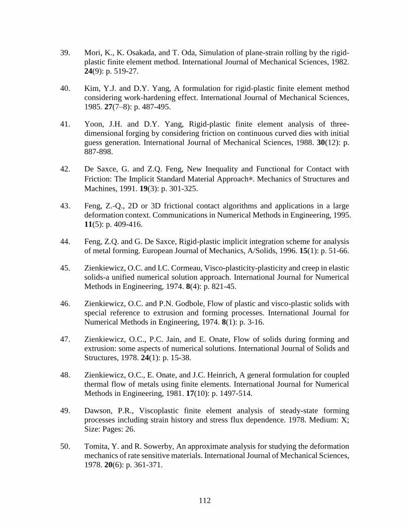
112

39. Mori, K., K. Osakada, and T. Oda, Simulation of plane-strain rolling by the rigid-

plastic finite element method. International Journal of Mechanical Sciences, 1982.

24(9): p. 519-27.

40. Kim, Y.J. and D.Y. Yang, A formulation for rigid-plastic finite element method

considering work-hardening effect. International Journal of Mechanical Sciences,

1985. 27(7–8): p. 487-495.

41. Yoon, J.H. and D.Y. Yang, Rigid-plastic finite element analysis of three-

dimensional forging by considering friction on continuous curved dies with initial

guess generation. International Journal of Mechanical Sciences, 1988. 30(12): p.

887-898.

42. De Saxce, G. and Z.Q. Feng, New Inequality and Functional for Contact with

Friction: The Implicit Standard Material Approach∗. Mechanics of Structures and

Machines, 1991. 19(3): p. 301-325.

43. Feng, Z.-Q., 2D or 3D frictional contact algorithms and applications in a large

deformation context. Communications in Numerical Methods in Engineering, 1995.

11(5): p. 409-416.

44. Feng, Z.Q. and G. De Saxce, Rigid-plastic implicit integration scheme for analysis

of metal forming. European Journal of Mechanics, A/Solids, 1996. 15(1): p. 51-66.

45. Zienkiewicz, O.C. and I.C. Cormeau, Visco-plasticity-plasticity and creep in elastic

solids-a unified numerical solution approach. International Journal for Numerical

Methods in Engineering, 1974. 8(4): p. 821-45.

46. Zienkiewicz, O.C. and P.N. Godbole, Flow of plastic and visco-plastic solids with

special reference to extrusion and forming processes. International Journal for

Numerical Methods in Engineering, 1974. 8(1): p. 3-16.

47. Zienkiewicz, O.C., P.C. Jain, and E. Onate, Flow of solids during forming and

extrusion: some aspects of numerical solutions. International Journal of Solids and

Structures, 1978. 24(1): p. 15-38.

48. Zienkiewicz, O.C., E. Onate, and J.C. Heinrich, A general formulation for coupled

thermal flow of metals using finite elements. International Journal for Numerical

Methods in Engineering, 1981. 17(10): p. 1497-514.

49. Dawson, P.R., Viscoplastic finite element analysis of steady-state forming

processes including strain history and stress flux dependence. 1978. Medium: X;

Size: Pages: 26.

50. Tomita, Y. and R. Sowerby, An approximate analysis for studying the deformation

mechanics of rate sensitive materials. International Journal of Mechanical Sciences,

1978. 20(6): p. 361-371.

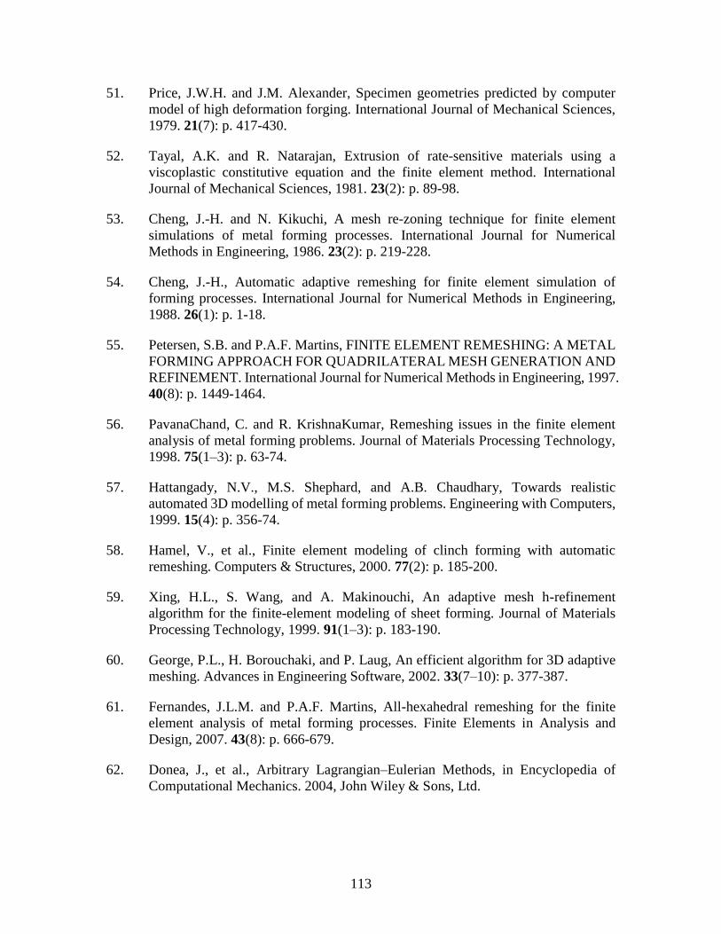
113

51. Price, J.W.H. and J.M. Alexander, Specimen geometries predicted by computer

model of high deformation forging. International Journal of Mechanical Sciences,

1979. 21(7): p. 417-430.

52. Tayal, A.K. and R. Natarajan, Extrusion of rate-sensitive materials using a

viscoplastic constitutive equation and the finite element method. International

Journal of Mechanical Sciences, 1981. 23(2): p. 89-98.

53. Cheng, J.-H. and N. Kikuchi, A mesh re-zoning technique for finite element

simulations of metal forming processes. International Journal for Numerical

Methods in Engineering, 1986. 23(2): p. 219-228.

54. Cheng, J.-H., Automatic adaptive remeshing for finite element simulation of

forming processes. International Journal for Numerical Methods in Engineering,

1988. 26(1): p. 1-18.

55. Petersen, S.B. and P.A.F. Martins, FINITE ELEMENT REMESHING: A METAL

FORMING APPROACH FOR QUADRILATERAL MESH GENERATION AND

REFINEMENT. International Journal for Numerical Methods in Engineering, 1997.

40(8): p. 1449-1464.

56. PavanaChand, C. and R. KrishnaKumar, Remeshing issues in the finite element

analysis of metal forming problems. Journal of Materials Processing Technology,

1998. 75(1–3): p. 63-74.

57. Hattangady, N.V., M.S. Shephard, and A.B. Chaudhary, Towards realistic

automated 3D modelling of metal forming problems. Engineering with Computers,

1999. 15(4): p. 356-74.

58. Hamel, V., et al., Finite element modeling of clinch forming with automatic

remeshing. Computers & Structures, 2000. 77(2): p. 185-200.

59. Xing, H.L., S. Wang, and A. Makinouchi, An adaptive mesh h-refinement

algorithm for the finite-element modeling of sheet forming. Journal of Materials

Processing Technology, 1999. 91(1–3): p. 183-190.

60. George, P.L., H. Borouchaki, and P. Laug, An efficient algorithm for 3D adaptive

meshing. Advances in Engineering Software, 2002. 33(7–10): p. 377-387.

61. Fernandes, J.L.M. and P.A.F. Martins, All-hexahedral remeshing for the finite

element analysis of metal forming processes. Finite Elements in Analysis and

Design, 2007. 43(8): p. 666-679.

62. Donea, J., et al., Arbitrary Lagrangian–Eulerian Methods, in Encyclopedia of

Computational Mechanics. 2004, John Wiley & Sons, Ltd.

114

63. Noh, W.F., CEL: A time-dependent, two-space-dimensional, Coupled Eulerian-

Lagrange code, in Methods in Computational Physics. 1964, Academic Press. p.

117-179.

64. Belytschko, T.B. and J.M. Kennedy, COMPUTER MODELS FOR

SUBASSEMBLY SIMULATION. Nuclear Engineering and Design, 1978. 49(1-

2): p. 17-38.

65. Hughes, T.J.R., W.K. Liu, and T.K. Zimmermann, Lagrangian-Eulerian finite

element formulation for incompressible viscous flows. Computer Methods in

Applied Mechanics and Engineering, 1981. 29(3): p. 329-349.

66. Wing Kam, L. and C. Hsiu Guo. A method of computation for fluid structure

interaction. in Symposium on Advances and Trends in Structures and Dynamics,

22-25 Oct. 1984. 1985. UK.

67. Casadei, F., et al., Transient fluid–structure interaction algorithms for large

industrial applications. Computer Methods in Applied Mechanics and Engineering,

2001. 190(24–25): p. 3081-3110.

68. Haber, R.B., A mixed Eulerian-Lagrangian displacement model for large-

deformation analysis in solid mechanics. Computer Methods in Applied Mechanics

and Engineering, 1984. 43(3): p. 277-92.

69. Liu, W.K., T. Belytschko, and H. Chang, An arbitrary Lagrangian-Eulerian finite

element method for path-dependent materials. Computer Methods in Applied

Mechanics and Engineering, 1986. 58(2): p. 227-45.

70. Schreurs, P.J.G., F.E. Veldpaus, and W.A.M. Brekelmans, Simulation of forming

processes, using the arbitrary eulerian-lagrangian formulation. Computer Methods

in Applied Mechanics and Engineering, 1986. 58(1): p. 19-36.

71. Ghosh, S. and N. Kikuchi, An arbitrary Lagrangian-Eulerian finite element method

for large deformation analysis of elastic-viscoplastic solids. Computer Methods in

Applied Mechanics and Engineering, 1991. 86(2): p. 127-188.

72. Benson, D.J., An efficient, accurate, simple ale method for nonlinear finite element

programs. Computer Methods in Applied Mechanics and Engineering, 1989. 72(3):

p. 305-350.

73. Wang, J. and M.S. Gadala, Formulation and survey of ALE method in nonlinear

solid mechanics. Finite Elements in Analysis and Design, 1997. 24(4): p. 253-269.

74. Gadala, M.S. and J. Wang, A practical procedure for mesh motion in arbitrary

Lagrangian-Eulerian method. Engineering with Computers, 1998. 14(3): p. 223-34.

115

75. Gadalaa, M.S., M.R. Movahhedy, and J. Wang, On the mesh motion for ALE

modeling of metal forming processes. Finite Elements in Analysis and Design,

2002. 38(5): p. 435-59.

76. Gadala, M.S., Recent trends in ALE formulation and its applications in solid

mechanics. Computer Methods in Applied Mechanics and Engineering, 2004.

193(39-41 SPEC. ISS.): p. 4247-4275.

77. Couch, R., et al. Application of ALE techniques to metal forming simulations. in

Proceedings of the 1993 ASME Winter Annual Meeting, November 28, 1993 -

December 3, 1993. 1993. New Orleans, LA, USA: Publ by ASME.

78. Gadala, M.S. and J. Wang, ALE formulation and its application in solid mechanics.

Computer Methods in Applied Mechanics and Engineering, 1998. 167(1-2): p. 33-

55.

79. Gadala, M.S. and J. Wang, Simulation of metal forming processes with finite

element methods. International Journal for Numerical Methods in Engineering,

1999. 44(10): p. 1397-1428.

80. Olovsson, L., L. Nilsson, and K. Simonsson, An ALE formulation for the solution

of two-dimensional metal cutting problems. Computers & Structures, 1999. 72(4–

5): p. 497-507.

81. Aymone, J.L.F., E. Bittencourt, and G.J. Creus, Simulation of 3D metal-forming

using an arbitrary Lagrangian–Eulerian finite element method. Journal of Materials

Processing Technology, 2001. 110(2): p. 218-232.

82. Boman, R., et al., Application of the Arbitrary Lagrangian Eulerian formulation to

the numerical simulation of cold roll forming process. Journal of Materials

Processing Technology, 2006. 177(1–3): p. 621-625.

83. Davey, K. and M.J. Ward, A practical method for finite element ring rolling

simulation using the ALE flow formulation. International Journal of Mechanical

Sciences, 2002. 44(1): p. 165-190.

84. Davey, K. and M.J. Ward, An ALE approach for finite element ring-rolling

simulation of profiled rings. Journal of Materials Processing Technology, 2003.

139(1–3): p. 559-566.

85. Gould, J.E. and Z. Feng, Heat flow model for friction stir welding of aluminum

alloys. Journal of Materials Processing and Manufacturing Science, 1998. 7(2): p.

185-194.

86. Frigaard, Grong, and O.T. Midling, A process model for friction stir welding of age

hardening aluminum alloys. Metallurgical and Materials Transactions A: Physical

Metallurgy and Materials Science, 2001. 32(5): p. 1189-1200.

116

87. Khandkar, M.Z.H., J.A. Khan, and A.P. Reynolds. A thermal model of the friction

stir welding process. in 2002 ASME International Mechanical Engineering

Congress and Exposition, November 17, 2002 - November 22, 2002. 2002. New

Orleans, LA, United states: American Society of Mechanical Engineers.

88. Khandkar, M.Z.H., J.A. Khan, and A.P. Reynolds, Prediction of temperature

distribution and thermal history during friction stir welding: input torque based

model. Science and Technology of Welding and Joining, 2003. 8(3): p. 165-174.

89. Chao, Y.J. and X. Qi, Thermal and thermo-mechanical modeling of friction stir

welding of aluminum alloy 6061-T6. Journal of Materials Processing and

Manufacturing Science, 1998. 7(2): p. 215-233.

90. Chao, Y.J., X. Qi, and W. Tang, Heat transfer in friction stir welding - Experimental

and numerical studies. Journal of Manufacturing Science and Engineering,

Transactions of the ASME, 2003. 125(1): p. 138-145.

91. Song, M. and R. Kovacevic, Thermal modeling of friction stir welding in a moving

coordinate system and its validation. International Journal of Machine Tools and

Manufacture, 2003. 43(6): p. 605-615.

92. Schmidt, H., J. Hattel, and J. Wert, An analytical model for the heat generation in

friction stir welding. Modelling and Simulation in Materials Science and

Engineering, 2004. 12(1): p. 143-57.

93. Schmidt, H.B. and J.H. Hattel, Thermal modelling of friction stir welding. Scripta

Materialia, 2008. 58(5): p. 332-337.

94. Hilgert, J., et al., Thermal models for bobbin tool friction stir welding. Journal of

Materials Processing Technology, 2011. 211(2): p. 197-204.

95. Ulysse, P., Three-dimensional modeling of the friction stir-welding process.

International Journal of Machine Tools and Manufacture, 2002. 42(14): p. 1549-

1557.

96. Colegrove, P.A. and H.R. Shercliff, 3-Dimensional CFD modelling of flow round

a threaded friction stir welding tool profile. Journal of Materials Processing

Technology, 2005. 169(2): p. 320-7.

97. Seidel, T.U., The development of a friction stir welding process model using

computational fluid dynamics. 2002, University of South Carolina.

98. Medhi, T., et al., Thermal modelling and effect of process parameters in friction

stir welding. Materials Today: Proceedings, 2015. 2(4–5): p. 3178-3187.

99. Sheppard, T. and D.S. Wright, Determination of flow stress: Part 1 constitutive

equation for aluminium alloys at elevated temperatures. Metals Technology, 1979.

6(1): p. 215-223.

117

100. Zener, C. and J.H. Hollomon, Effect of Strain Rate Upon Plastic Flow of Steel.

Journal of Applied Physics, 1944. 15(1): p. 22-32.

101. Seidel, T.U. and A.P. Reynolds, Two-dimensional friction stir welding process

model based on fluid mechanics. Science and Technology of Welding and Joining,

2003. 8(3): p. 175-183.

102. Colegrove, P.A. and H.R. Shercliff, Experimental and numerical analysis of

aluminium alloy 7075-T7351 friction stir welds. Science and Technology of

Welding and Joining, 2003. 8(5): p. 360-368.

103. Colegrove, P.A. and H.R. Shercliff, CFD modelling of friction stir welding of thick

plate 7449 aluminium alloy. Science and Technology of Welding and Joining, 2007.

11(4): p. 429-41.

104. Long, T. and A.P. Reynolds, Parametric studies of friction stir welding by

commercial fluid dynamics simulation. Science and Technology of Welding and

Joining, 2007. 11(2): p. 200-8.

105. Nandan, R., G.G. Roy, and T. Debroy, Numerical simulation of three dimensional

heat transfer and plastic flow during friction stir welding. Metallurgical and

Materials Transactions A: Physical Metallurgy and Materials Science, 2006. 37(4):

p. 1247-1259.

106. Nandan, R., et al., Numerical modelling of 3D plastic flow and heat transfer during

friction stir welding of stainless steel. Science and Technology of Welding and

Joining, 2006. 11(5): p. 526-37.

107. Nandan, R., et al., Three-dimensional heat and material flow during friction stir

welding of mild steel. Acta Materialia, 2007. 55(3): p. 883-895.

108. Atharifar, H., L. Dechao, and R. Kovacevic, Numerical and Experimental

Investigations on the Loads Carried by the Tool During Friction Stir Welding.

Journal of Materials Engineering and Performance, 2009. 18(4): p. 339-50.

109. Cox, C., et al., Modeling the control of an elevated tool temperature and the affects

on axial force during friction stir welding. Materials and Manufacturing Processes,

2010. 25(11): p. 1278-1282.

110. Aljoaba, S., et al., Modeling the Effects of Coolant Application in Friction Stir

Processing on Material Microstructure Using 3D CFD Analysis. Journal of

Materials Engineering and Performance, 2012. 21(7): p. 1141-50.

111. Hasan, A.F., C.J. Bennett, and P.H. Shipway, A numerical comparison of the flow

behaviour in Friction Stir Welding (FSW) using unworn and worn tool geometries.

Materials & Design, 2015. 87: p. 1037-1046.

118

112. Su, H., et al., Numerical modeling for the effect of pin profiles on thermal and

material flow characteristics in friction stir welding. Materials & Design, 2015. 77:

p. 114-125.

113. Xu, S., et al., Finite element simulation of material flow in friction stir welding.

Science and Technology of Welding and Joining, 2001. 6(3): p. 191-193.

114. Deng, X. and S. Xu, Two-Dimensional Finite Element Simulation of Material Flow

in the Friction Stir Welding Process. Journal of Manufacturing Processes, 2004.

6(2): p. 125-133.

115. Schmidt, H. and J. Hattel, A local model for the thermomechanical conditions in

friction stir welding. Modelling and Simulation in Materials Science and

Engineering, 2005. 13(1): p. 77-93.

116. Assidi, M., et al., Friction model for friction stir welding process simulation:

Calibrations from welding experiments. International Journal of Machine Tools and

Manufacture, 2010. 50(2): p. 143-155.

117. van der Stelt, A.A., et al. Comparison of ALE finite element method and adaptive

smoothed finite element method for the numerical simulation of friction stir

welding. in 14th International Esaform Conference on Material Forming: Esaform

2011, 27-29 April 2011. 2011. USA: American Institute of Physics.

118. Liu, X., S. Lan, and J. Ni, Thermal Mechanical Modeling of the Plunge Stage

During Friction-Stir Welding of Dissimilar Al 6061 to TRIP 780 Steel. Journal of

Manufacturing Science and Engineering, 2015. 137(5): p. 051017-051017.

119. Zhang, H.W., Z. Zhang, and J.T. Chen, 3D modeling of material flow in friction

stir welding under different process parameters. Journal of Materials Processing

Technology, 2007. 183(1): p. 62-70.

120. Grujicic, M., et al., Fully coupled thermomechanical finite element analysis of

material evolution during friction-stir welding of AA5083. Proceedings of the

Institution of Mechanical Engineers, Part B (Journal of Engineering Manufacture),

2010. 224(B4): p. 609-25.

121. Chiumenti, M., et al., Numerical modeling of friction stir welding processes.

Computer Methods in Applied Mechanics and Engineering, 2013. 254: p. 353-369.

122. Pan, W., et al., A new smoothed particle hydrodynamics non-Newtonian model for

friction stir welding: Process modeling and simulation of microstructure evolution

in a magnesium alloy. International Journal of Plasticity, 2013. 48: p. 189-204.

123. Grujicic, M., et al., Computational Analysis of Material Flow During Friction Stir

Welding of AA5059 Aluminum Alloys. Journal of Materials Engineering and

Performance, 2012. 21(9): p. 1824-40.

119

124. Neto, D.M. and P. Neto, Numerical modeling of friction stir welding process: a

literature review. International Journal of Advanced Manufacturing Technology,

2013. 65(1-4): p. 115-26.

125. He, X., F. Gu, and A. Ball, A review of numerical analysis of friction stir welding.

Progress in Materials Science, 2014. 65: p. 1-66.

126. Sinnott, R.K., Chemical Engineering Design: Chemical Engineering. 2005:

Elsevier Science.

127. Abramowitz, M. and I.A. Stegun, Handbook of Mathematical Functions: With

Formulas, Graphs, and Mathematical Tables. 1964: Dover Publications.

128. Versteeg, H.K. and W. Malalasekera, An Introduction to Computational Fluid

Dynamics: The Finite Volume Method. 2007: Pearson Education Limited.

129. Zhang, H., et al., Investigation of material flow during friction extrusion process.

International Journal of Mechanical Sciences, 2014. 85: p. 130-141.

130. Zhao, X., et al., Stereo image based motion measurements in fluids: experimental

validation and application in friction extrusion. Experimental Mechanics, 2015.

55(1): p. 177-200.

131. Zhang, H., et al., Heat transfer modeling of the friction extrusion process. Journal

of Materials Processing Technology, 2015. 221: p. 21-30.

132. Li, X., W. Tang, and A.P. Reynolds, Material Flow and Texture in Friction

Extruded Wire, in Friction Stir Welding and Processing VII. 2013, John Wiley &

Sons, Inc. p. 339-347.

133. Li, X., et al., Strain and texture in friction extrusion of aluminum wire. Journal of

Materials Processing Technology, 2016. 229: p. 191-198.

134. Valberg, H. and T. Malvik, An experimental investigation of the material flow

inside the bearing channel in aluminium extrusion. International Journal of

Materials and Product Technology, 1994. 9(4-6): p. 428-463.

135. Mukai, T., K. Ishikawa, and K. Higashi, Influence of strain rate on the mechanical

properties in fine-grained aluminum alloys. Materials Science and Engineering: A,

1995. 204(1–2): p. 12-18.

136. Malas, J.C. and V. Seetharaman, Using material behavior models to develop

process control strategies. JOM, 1992. 44(6): p. 8-13.

137. Balasubrahmanyam, V.V. and Y.V.R.K. Prasad, Hot deformation mechanisms in

Ti-5.5Al-1Fe alloy. Journal of Materials Engineering and Performance, 2001. 10(6):

p. 731-9.

120

138. Lin, Y.C., et al., Constitutive descriptions for hot compressed 2124-T851 aluminum

alloy over a wide range of temperature and strain rate. Computational Materials

Science, 2010. 50(1): p. 227-233.

139. Sheppard, T., Extrusion of AA 2024 alloy. Materials Science and Technology, 1993.

9(5): p. 430-440.

140. Clade, M.P. and T. Sheppard, Extrusion limit diagrams containing structural and

topological information for AA 6063 aluminium alloy. Materials Science and

Technology, 1993. 9(4): p. 313-318.

141. Sheppard, T. and A. Jackson, Constitutive equations for use in prediction of flow

stress during extrusion of aluminium alloys. Materials Science and Technology,

1997. 13(3): p. 203-209.

142. Duan, X. and T. Sheppard, The influence of the constitutive equation on the

simulation of a hot rolling process. Journal of Materials Processing Technology,

2004. 150(1–2): p. 100-106.

143. Lesuer, D.R., G.J. Kay, and M.M. LeBlanc. Modeling large strain, high rate

deformation in metals. in Modelling the Performance of Engineering Structural

Materials II. Proceedings of a Symposium, 4-8 Nov. 2001. 2001. Warrendale, PA,

USA: TMS - Miner. Metals &amp; Mater. Soc.

144. Doude, H.R., J.A. Schneider, and A.C. Nunes, Influence of the Tool Shoulder

Contact Conditions on the Material Flow During Friction Stir Welding.

Metallurgical and Materials Transactions A, 2014. 45(10): p. 4411-22.

145. Wang, H., P.A. Colegrove, and J.F. dos Santos, Numerical investigation of the tool

contact condition during friction stir welding of aerospace aluminium alloy.

Computational Materials Science, 2013. 71: p. 101-108.

146. Chang, C.I., C.J. Lee, and J.C. Huang, Relationship between grain size and Zener–

Holloman parameter during friction stir processing in AZ31 Mg alloys. Scripta

Materialia, 2004. 51(6): p. 509-514.

147. Wang, Y.N., et al. Influence from extrusion parameters on high strain rate and low

temperature superplasticity of AZ series Mg-based alloys. in THERMEC'2003.

International Conference on Processing and Manufacturing of Advanced Materials,

7-11 July 2003. 2003. Switzerland: Trans Tech Publications.

148. Ammouri, A.H., et al., Relating grain size to the Zener–Hollomon parameter for

twin-roll-cast AZ31B alloy refined by friction stir processing. Journal of Materials

Processing Technology, 2015. 222: p. 301-306.

149. Duan, X. and T. Sheppard. Influence of forming parameters on the final subgrain

size during hot rolling of aluminium alloys. 2002. Elsevier Ltd.

121

150. Robson, J.D. and L. Campbell, Model for grain evolution during friction stir

welding of aluminium alloys. Science and Technology of Welding and Joining,

2010. 15(2): p. 171-176.

151. Morisada, Y., T. Imaizumi, and H. Fujii, Determination of strain rate in Friction

Stir Welding by three-dimensional visualization of material flow using X-ray

radiography. Scripta Materialia, 2015. 106: p. 57-60.

122

APPENDIX A USER DEFINED FUNCTIONS

Viscosity

The viscosity of AA6061 is implemented by a user defined function. It is a function

of temperature and strain rate. The strain rate is not smaller than 10-4 /s and the viscosity is

not larger than 1012 /s. The user defined function is written in C and to be complied by

FLUENT.

# include "udf.h"

DEFINE_PROPERTY(visco6061, c, t)

{

real visco;

real tp;

real s_rate = C_STRAIN_RATE_MAG(c,t);

real a;

real n;

real q;

real r;

real b;

real z;

a = 4.5e-8;

n = 3.55;

q = 145000.0;

123

r = 8.314;

b=exp(19.3);

tp = C_T(c, t);

if( s_rate <= 1.0e-4) s_rate = 1.0e-4;

z = s_rate * exp(q / (r * tp));

visco=1 / (3 * a * s_rate) * log(pow((z / b),1.0 / n)+pow((pow((z / b), 2.0 / n)+1), 0.5));

if(visco >=1.0e12) visco=1.0e12;

return visco;

}

Rotating Speed

The rotating speed of the die increases from zero to 300 rpm and the increase is

controlled by a user defined function as follows.

The following is for x-direction.

# include "udf.h"

DEFINE_PROFILE(v_x, t,i)

{

face_t f;

real x[ND_ND];

real xx, yy,r;

real theta;

real tm;

real w;

real vx;

124

tm=CURRENT_TIME;

if (tm>=0 && tm<=4.7)

w=0;

else if (tm>4.7 && tm<8.7)

w=(tm-4.7)*7.855*0.6;

else

w=31.42*0.6;

vx=0;

begin_f_loop(f,t)

{

F_CENTROID(x,f,t);

xx=x[0];

yy=x[1];

r=sqrt(xx*xx+yy*yy);

if (xx!=0) theta=atan(fabs(yy)/fabs(xx));

if(yy>0 && xx!=0)

vx=-w*r*sin(theta);

else if(yy>0&&xx==0)

vx=-w*r;

else if (yy==0)

vx=0;

else if(yy<0 && xx!=0)

vx=w*r*sin(theta);

125

else

vx=w*r;

F_PROFILE(f,t,i)=vx;

}

end_f_loop(f,t)

}

The following is for y-direction.

# include "udf.h"

DEFINE_PROFILE(v_y, t,i)

{

face_t f;

real x[ND_ND];

real xx, yy,r;

real theta;

real tm;

real w;

real vy;

vy=0;

tm=CURRENT_TIME;

if (tm>=0 && tm<=4.7)

w=0;

else if (tm>4.7 && tm<8.7)

126

w=(tm-4.7)*7.855*0.6;

else

w=31.42*0.6;

begin_f_loop(f,t)

{

F_CENTROID(x,f,t);

xx=x[0];

yy=x[1];

r=sqrt(xx*xx+yy*yy);

if (xx!=0) theta=atan(fabs(yy)/fabs(xx));

if(xx>0)

vy=w*r*cos(theta);

else if (xx==0)

vy=0;

else

vy=-w*r*cos(theta);

F_PROFILE(f,t,i)=vy;

}

end_f_loop(f,t)

}

Moving Mesh

The reduction of the volume of the fluid computational domain is by moving the domain

and the dynamic meshing. The user defined function for the motion is as follows.

127

#include"udf.h"

DEFINE_CG_MOTION(dyn,dt,cg_vel,cg_omega,time,dtime)

{

cg_vel[0]=0;

cg_vel[1]=0;

NV_S(cg_omega,=,0.0);

if(time >10 && time <=24.5)

cg_vel[2]=-1.12e-4;

else if(time>24.5 && time<28)

cg_vel[2]=-1.85e-5;

else

cg_vel[2]=0;

}

Simulation of the Gap

The gap between the chamber wall and the aluminum alloy sample is simulated by

changing the conductivity of the gap region. The following is the user defined function.

# include "udf.h"

DEFINE_PROPERTY(cond,c,t)

{

real tm;

real tp;

real cond;

128

real h1;

real h2;

real x[ND_ND];

real xx,yy,rr,zz;

tm=CURRENT_TIME;

tp=C_T(c,t);

F_CENTROID(x,c,t);

xx=x[0];

yy=x[1];

zz=x[2];

rr=sqrt(xx*xx+yy*yy);

if (rr>=0.01275)

{if(tm>0 && tm<5)

cond=2;

else if( tm>=5 && tm<=10)

{

h1=0.019+0.00204*(tm-5);

h2=0.018-0.0036*(tm-5);

if(zz>h2 && zz<h1)

cond=115+0.1594*tp;

else

cond=2;

}

129

else

cond=115+0.1594*tp;

}

else

cond=35;

return cond;

}

Heat Source

The heat generation rate in the volume heating layer is linear along both radial and vertical

directions. The mechanical power curve correlated to the heat generation rate is fitted by

polynomials. The user defined function for it is as follows

#include "udf.h"

DEFINE_SOURCE(qua,c,t,ds,eqn)

{

real x[ND_ND];

real xx;

real yy;

real zz;

real r;

real h;

real w;

real source;

real tm;

130

real alpha;

real dd;

real a1, b1,c1,d1;

real a2, b2,c2,d2,e2;

real a3, b3,c3,d3;

real a4,b4,c4,d4;

real t1,t2,t3,t4,t5;

alpha=1;

a1=0.0816;

b1=0.0159;

c1=-0.3628;

d1=0.1097;

a2=-0.1429;

b2=3.2986;

c2=-28.03;

d2=104.49;

e2=-139.71;

a3=-0.001;

b3=0.064;

c3=-1.4098;

d3=14.183;

a4=-0.0268;

131

b4=2.5283;

c4=-79.602;

d4=837.77;

t1=0;

t2=4;

t3=7.5;

t4=27.7;

t5=31;

tm=CURRENT_TIME;

F_CENTROID(x,c,t);

xx=x[0];

yy=x[1];

zz=x[2];

r=sqrt(xx*xx+yy*yy);

if(tm>=0 && tm<=10)

dd=0;

else if(tm >10 && tm <=24.5)

dd=(tm-10)*1.12e-4;

else

dd=1.624e-3;

h=zz-0.015+dd;

if(tm>t1 && tm<=t2)

{

132

w=(a1*pow(tm,3)+b1*pow(tm,2)+c1*pow(tm,1)+d1)*1000;

if(w<=0) w=0;

}

else if ( tm> t2 && tm <= t3)

w=(a2*pow(tm,4)+b2*pow(tm,3)+c2*pow(tm,2)+d2*pow(tm,1)+e2)*1000;

else if( tm> t3 && tm<=t4)

w=(a3*pow(tm,3)+b3*pow(tm,2)+c3*pow(tm,1)+d3)*1000;

else if( tm> t4 && tm<=t5)

w=(a4*pow(tm,3)+b4*pow(tm,2)+c4*pow(tm,1)+d4)*1000;

else

w=0;

if( h>0)

source = alpha*w*r*h*3/98125*1e15;

else

source=0;

return source;

}