Numerical Methods For American Options · 2008-04-14 · Figure 1.1: Payoﬀ Diagram for a European...

Numerical Methods For American Options

S.C.Benbow

August 22, 2005

Abstract

The problem of solving the Black-Scholes equation for the valuation of Amer-

ican options is tackled using a Crank-Nicolson finite difference method for-

mulated in a Lagrangian frame.

We firstly introduce a transformation to convert the Black-Scholes equation

into a dimensionless constant coefficient forward equation. We then formu-

late the equation is the moving Lagrangian reference frame. The problem of

solving the Black-Scholes equation for American options is treated as a free

boundary problem, where we must determine both the value of the option,

and also when the option should be exercised. We introduce a new method

for locating the moving boundary. The equation is then solved using a finite

difference Crank-Nicolson method.

A monitor function is introduced to increase the resolution of the method

close to the exercise boundary, and the method is modified to accommodate

this. We then attempt to solve the problem using a finite element method

and compare the accuracy of the two approaches.

Acknowledgements

I would like to thank Prof. M.J.Baines for his time and invaluable help with

this thesis. I have thoroughly enjoyed working with him, this dissertation has

given me an insight into the true nature of research and provided me with

motivation to continue with my studies. I would also like to acknowledge my

colleagues on the Msc course and the other members of the academic staff in

the Department of mathematics at the University of Reading.

This year has been both enjoyable and challenging. I would like to thank my

family, especially me wife, for all of their support and hard work in the last

twelve months in allowing me to study at Reading and take full advantage

of this wonderful opportunity.

1

Contents

1 Introduction 4

1.1 The Problem . . . . . . . . . . . . . . . . . . . . . . . . . . . 4

1.2 Aims . . . . . . . . . . . . . . . . . . . . . . . . . . . . . . . . 6

2 Background 8

2.1 Model for Asset Prices . . . . . . . . . . . . . . . . . . . . . . 8

2.2 Black-Scholes Model . . . . . . . . . . . . . . . . . . . . . . . 10

2.3 Black-Scholes For European Option . . . . . . . . . . . . . . . 13

2.4 Modification to the model . . . . . . . . . . . . . . . . . . . . 14

2.5 American Option . . . . . . . . . . . . . . . . . . . . . . . . . 18

2.6 American Call with Dividends . . . . . . . . . . . . . . . . . . 20

2.7 General Analysis of Call with Dividends . . . . . . . . . . . . 21

3 Transformation 25

3.1 American Options PDE . . . . . . . . . . . . . . . . . . . . . 25

3.2 Transformation to Diffusion Equation . . . . . . . . . . . . . . 26

4 Numerical Methods 28

4.1 Finite Difference Based Front Tracking Method . . . . . . . . 28

4.2 Invertbility . . . . . . . . . . . . . . . . . . . . . . . . . . . . 35

2

4.3 Stability Analysis . . . . . . . . . . . . . . . . . . . . . . . . . 36

4.4 Local Analysis of the Free Boundary . . . . . . . . . . . . . . 38

4.5 Derivative Boundary Conditions . . . . . . . . . . . . . . . . 40

4.6 Description of Algorithm 1 . . . . . . . . . . . . . . . . . . . . 41

4.7 Algorithm 2 . . . . . . . . . . . . . . . . . . . . . . . . . . . . 43

4.8 Invertbility-method two . . . . . . . . . . . . . . . . . . . . . 46

4.9 Description of Algorithm 2 . . . . . . . . . . . . . . . . . . . . 46

5 Finite Element Method 49

5.1 Introduction . . . . . . . . . . . . . . . . . . . . . . . . . . . . 49

5.2 Weak Form . . . . . . . . . . . . . . . . . . . . . . . . . . . . 51

5.3 Finite Elements Algorithm . . . . . . . . . . . . . . . . . . . . 53

6 Results 55

6.1 Finite Differences . . . . . . . . . . . . . . . . . . . . . . . . . 55

6.2 Finite Element Algoritm . . . . . . . . . . . . . . . . . . . . . 63

7 conclusion 65

8 Reference 67

.1 Program 1 - pt1.f90 . . . . . . . . . . . . . . . . . . . . . . . . 69

.2 Program 2 - pt2.f90 . . . . . . . . . . . . . . . . . . . . . . . . 84

.3 Program 3 - pt3.f90 . . . . . . . . . . . . . . . . . . . . . . . . 95

3

Chapter 1

Introduction

1.1 The Problem

The simplest financial option, a European call option, is a contract with the

following conditions

• At a prescribed time in the future, known as the expiry date the holder

of the option may do the following;

• purchase a prescribed asset, known as the underlying for a

• prescribed amount, known as the exercise price or strike price

For the holder of the option, the contract is a right but not an obligation.

The other party to the contract, the individual who is known as the writer

does have a potential obligation, he must sell the asset if the holder chooses

to buy it.

The option confers to its holder a right without an obligation, and there-

fore has intrinsic value.

4

The main concerns in the valuation of options are:

• How much would one pay for this right, i.e. what is the value of an

option?

• How can the writer minimize the risk associated with his obligation?

Options have become extremely popular recently, primarily because they are

attractive to investors, both for speculation and for hedging, and because

there is now a systematic way to determine how much they are worth.

We let E denote the exercise price, i.e the cost of purchasing the option,

and S(T ) denote the underlying asset price at the expiry date. At expiry if

S(T ) > E then the holder of the call option may buy that asset for E and

then immediately sell it in the market for S(T ), gaining an amount S(T )−E.

Conversely, if E ≥ S(T ) then the holder gains nothing. The value of the call

option may therefore be expressed as

C = max(S(T ) − E, 0) (1.1.1)

Plotting S(T ) on the x-axis and C on the y-axis gives a payoff diagram as

shown in 1.1.

American options have the additional feature that exercise is permitted at

any time during the life of the option. This is in contrast to a European

option which may only be exercised at expiry. Since the American option

gives its holder greater rights than the European option, via the right of early

5

Figure 1.1: Payoff Diagram for a European Call

exercise, potentially it has a higher value. This report will focus on the valu-

ation of American options, which are mathematically more interesting than

their European counterparts since they can be interpreted as free boundary

problems.

The American option valuation problem can be shown to be uniquely spec-

ified by a series of constraints, which are similar to those of an ’obstacle’

problem. Since we do not know the location of the free boundary Sf (t) a

priori we are lacking one piece of information compared with the European

options. Not only must a value be assigned to the option but, we must also

determine when it is best to exercise the option.

1.2 Aims

The aims of this dissertation are to produce an accurate method for the val-

uation of American call options. The optimal exercise boundary is modeled

6

by a moving boundary. The time dependent boundary point is physically in-

terpreted as the division between two regions, one where we should hold the

option, and the other where we should exercise. This point is known as the

optimal exercise price. We seek a method which will determine accurately

the location of this free boundary, and furthermore provide a corresponding

valuation for the option at discrete time steps up until the expiry date.

The conventional approach is to transform the Black-Scholes equation into a

dimensionless parabolic equation and then discretise the problem using nu-

merical methods to find a solution1. We propose a new method of solution,

in which the equations are discretised on a moving grid. Since the optimal

exercise boundary is time dependent, and found to increase in time for the

case of a call, we also propose a new technique for expanding the domain.

Finally, we intend to solve same the problem using a finite element approach,

and compare the accuracy between the two schemes.

1see K.N PANAZOPOULOS ET AL

7

Chapter 2

Background

2.1 Model for Asset Prices

In order to value an option we must develop a mathematical description

of how the underlying asset behaves. The price of an asset is a measure

of investors confidence. Although an oversimplification, it is reasonable to

assume that the market responds instantaneously to external influences. Fur-

thermore asset prices must move randomly because of the efficient market

hypothesis. This can be stated as

• The past history is fully reflected in the present price, which does not

hold any further information

• Markets respond immediately to any new information about an asset

With these two assumptions, the asset price is said to follow a Markov pro-

cess

8

Definition 1. A Markov process is a particular type of stochastic process

where only the present value of a variable is relevant in predicting the future.

The past history of the variable, and the way in which the present has emerged

from the past are irrelevant

Suppose that at time t the asset price is S. Consider a small subsequent

time interval dt, during which S changes to S + dS. We decompose this

return into two parts, one component that is deterministic, comparable to

the return on a risk-free investment. This gives contribution to the return

dS/S

µdt (2.1.1)

µ is a measure of the average rate of growth of the asset price, also known

as drift.

The second contribution to dS/S models the random change in the asset

price in response to external effects. It is represented by a random sample

drawn from a normal distribution with mean zero. It adds contribution

σdX (2.1.2)

σ is known as the volitility, which measures the standard deviation of the

returns.

Putting the two together yields the Stochastic Differential Equation

dS

S= σdX + µdt (2.1.3)

This is the basic mathematical representation for generating asset prices.

The term dX, which contains the random element which is a feature of asset

9

prices, is known as a Wiener process, it has the following properties:

• dX is a random variable, drawn from a normal distribution

• dX has a mean of zero and a variance dt

This may be expressed as

dX = φ√

dt (2.1.4)

φ is a random variable drawn from a standardized normal distribution, with

zero mean and variance of one. The probability distribution function is given

by

1√2π

e−12φ2

(2.1.5)

A generalized Wiener process with drift µ and variance σ is shown in figure

2.1

2.2 Black-Scholes Model

The key question concerning the valuation of Options is: what is an option

worth at time t=0? The problem is to systematically determine a fair value

for an option, at the time at which the contract is entered into. Before we

proceed with any analysis, there are several assumptions that we must first

make

• The asset price follows a log normal random walk

• The risk-free interest rate r and the asset volatility σ are known func-

tions of time over the life of the option.

10

• There are no associated transaction costs

• The underlying asset pays no dividends during the life of the option.

• There are no arbitrage possibilities

• Trading of the underlying asset can take place continuously

We now look for a function V (S, t) that gives the option value for any asset

price S ≥ 0 and at any time 0 ≤ t ≤ T . In this setting, V (S0, 0) is the

required time-zero option value. We further assume that such a function

exists and is smooth in both variables. Ito’s Lemma provides us with a

derivative chain rule for stochastic functions; i.e. if f = f(W, t) where W is

some stochastic function.

df =df

dS(σSdX + µSdt) +

1

2σ2S2 d2f

dS2dt (2.2.1)

Using 2.2.1 we can write

dV = σSdV

dSdX +

(

µS∂V

∂S+

1

2σ2S2∂2V

∂S2+

∂V

∂t

)

dt (2.2.2)

This gives the random walk followed by V .

We now construct a portfolio consisting of one option and a proportion −∆

of the underlying asset. The value of the portfolio is

Π = V − ∆S (2.2.3)

The change in the value of this portfolio in one time-step is

dΠ = dV − ∆dS (2.2.4)

11

Combining 2.1.3, 2.2.2 and 2.2.3 we find that Π follows the random walk

dΠ = σS

(

∂V

∂S− ∆

)

dX +

(

µS∂V

∂S+

1

2σ2S2 ∂2

∂S2+

∂V

∂t− µ∆S

)

dt (2.2.5)

We can eliminate the random component by choosing ∆ = ∂V∂S

. This results

in a portfolio whose increment is wholly deterministic

dΠ =

(

∂V

∂t+

1

2σ2S2∂2V

∂S2

)

dt (2.2.6)

The return on on an amount Π invested in a risk less asset would see a growth

of rΠdt in a time dt. If the right hand side of 2.2.6 were greater than this

amount, an arbitrager could make a guaranteed risk less profit by borrowing

an amount Π to invest in the portfolio. Conversely, if the right-hand side of

2.2.6 were less than rΠdt then the arbitrager would make a risk less, no cost,

instantaneous profit.

Thus we have

rΠdt =

(

∂V

∂t+

1

2σ2S2∂2V

∂S2

)

dt (2.2.7)

Substituting 2.2.3 and ∆ = ∂V∂S

into 2.2.7 and dividing by dt we arrive at the

Black-Scholes partial differential equation

∂V

∂t+

1

2σ2S2∂2V

∂S2+ rS

∂V

∂S− rV = 0 (2.2.8)

Any derivative security whose price depends only on the current value of S

and on t, which is paid for up-front, must satisfy the Black-Scholes equation.

12

2.3 Black-Scholes For European Option

The Black-Scholes equation 2.2.8 is a backward parabolic equation. We must

therefore impose boundary conditions to ensure a unique solution. We must

impose two conditions on S, and one on t. For example we may specify that

V (S, t) = Va(t) on S = a and also that V (S, t) = Vb(t) on S = b.

Since the equation is backward in time we must also impose a final condition

such as

V (S, t) = VT (S) on t = T (2.3.1)

Where VT is a known function of time.

In the case of European options, in particular the European call, we de-

note the call value by C(S, t), with exercise price E and expiry date T .

At time t = T , the value of the call is known for certainty to be

C(S, T ) = max(S − E, 0) (2.3.2)

This is the final condition.

If S = 0 at expiry then the payoff is zero, the call option is therefore worthless,

even if there is still a period of time until expiry.

C(0, t) = 0 (2.3.3)

As the asset price increases, it will become more likely that the option will

be exercised and the actual magnitude of the exercise price becomes less

13

important. We can therefore write that as S → ∞ the value of the option

becomes that of the asset

C(S, t) S as S → ∞ (2.3.4)

For the European options, without the possibility of early exercise 2.2.8 can

be solved exactly to give the Black-Scholes value of the call option.

Assuming that the interest rate and the volatility are constant, the explicit

solution for the European call is

C(S, t) = SN(d1) − Ee−r(T−t)N(d2) (2.3.5)

N is a cumulative distribution function for a standardized normal random

variable, given by

N(x) =1√2π

∫ x

−∞

e−12y2

dy (2.3.6)

d1 =log(S/E) + (r + 1

2σ2)(T − t)

σ√

T − t(2.3.7)

d2 =log(S/E) + (r − 1

2σ2)(T − t)

σ√

T − t(2.3.8)

Figure 2.3 below shows a European call value C(S, t) as a function of S for

several values of time to expiry, with r = 0.1 and σ = 0.2

2.4 Modification to the model

In this dissertation we attempt to model the price of American options based

on dividend paying assets. The model introduced in the previous section

makes the simplification that no dividends are paid. We now consider the

14

Figure 2.1: American Call Value Prior to expiry

effect on the options price when dividend payment is incorporated into the

model.

When assets pay out dividends, the price of an option on a underlying asset is

affected by the payments. A modification must be made to the black-scholes

equation.

In modeling dividends we must ask two questions:

• When and how often are dividend payments made?

• How large are the dividend payments?

The amounts paid as dividends may be modeled as either deterministic or

stochastic. In this dissertation we consider only those equities with dividends

whose amount and timing is known at the start of the options life.

Suppose that in time dt the underlying asset pays out a dividend D0Sdt

where D0 is a constant. The payment is independent of time, but dependent

15

on the stock price S. The Dividend Yield is defined as the proportion of the

asset price that is paid out per unit time in this way.

Arbitrage considerations show that in each time-step dt, the asset price must

fall by the amount of the dividend payment, in addition to the usual fluctu-

ations. The random walk of the asset price 2.1.3 is modified to become

dS = σSdX + (µ − D0)Sdt (2.4.1)

Considering the effect of the dividend payments on our hedged portfolio, we

receive and amount D0Sdt for every asset held, and since we hold −∆ of the

underlying, the portfolio changes by an amount

−D0S∆dt (2.4.2)

Adding 2.4.2 to 2.2.4 we arrive at

dΠ = dV − ∆dS − D0S∆dt (2.4.3)

Following the same analysis as previously we obtain

∂V

∂t+

1

2σ2S2∂2V

∂S2+ (r − D0)S

∂V

∂S− rV = 0 (2.4.4)

The only change to the boundary conditions is that

C(S, t) Se−D0(T−t) as S → ∞ (2.4.5)

The value of a European call with dividends can be shown to be

C(S, t) = e−D0(T−t)SN(d10) − Ee−r(T−t)N(d20) (2.4.6)

Where

d10 =log(S/E) + (r − D0 + 1

2σ2)(T − t)

σ√

T − t(2.4.7)

d20 = d1 − σ√

T − t (2.4.8)

16

Figure 2.2: European Option Values with (lower) and without (lower) divi-

dends

17

2.5 American Option

American Options have the important additional feature that early exercise

is permitted at any time during the life of the option.

Definition 2. An American Call Option gives its holder the right, but not

the obligation, to purchase from the writer a prescribed asset for a prescribed

price at any time between the start date and a prescribed expiry date in the

future.

The formulae in section 2.3 and 2.4 do not necessarily agree with the

value of American options. The ability to exercise the option at any time

extends to the owner additional rights, and thus the American option has

potentially a higher value.

If S lies in this range so that P (S, t) < max(E − S, 0) and we exercise

the option, there is an obvious arbitrage opportunity. We could buy the as-

set in the market immediately for S and at the same time buy the option for

P ; if we then exercised the option by selling the asset for E we make a risk

free profit of E − P − S.

This opportunity would not last long before the value of the option was

pushed up by the demand of the arbitragers. We must therefore conclude

that when early exercise is permitted we must impose the constraint

V (S, t) ≥ max(S − E, 0) (2.5.1)

American and European options must therefore have different values.

18

In the case of American options there are some values of S for which it

is optimal from the holders point of view to exercise the American option. If

this were not the case the option would have the same value as the European

option, the Black-Scholes equation would hold for all S.

The valuation of an American option is therefore more complicated than

its European counterpart since we have to determine not only the option

value but also, for each value of S, whether or not it should be exercised.

This is what is known as a free boundary problem. At each time t there

is a particular value of S which marks the boundary between two regions: to

one side one should hold the option and to the other side one should exercise

it.

We denote this value, which varies with time, by Sf (t), and refer to it as

the optimal exercise price.

As we have already observed, since we do not know Sf a priori unlike the cor-

responding European problem, we do not know where to apply the boundary

conditions, and for this reason, the problem is called a free boundary problem.

An American option valuation can be shown to be uniquely specified by

a set of constraints

• the option value must be greater than or equal to the payoff function

• the Black-Scholes equation is replaced by an inequality

19

• the option value must be a continuous function of S

• the option delta (slope) must be continuous

2.6 American Call with Dividends

From section 2.2 the value C(S, t) of an American option satisfies

∂C

∂t+

1

2σ2S2∂2C

∂S2+ (r − D0)S

∂C

∂S− rC = 0 (2.6.1)

This holds as long as exercise is not optimal. The payoff condition is

C(S, T ) = max(S − E, 0) (2.6.2)

Also, since the option may be exercised at any time, we have that

C(S, t) ≥ max(S − E, 0) (2.6.3)

Along the optimal exercise boundary S = Sf (t)

C(Sf (t), t) = Sf (t) − E∂C

∂S(Sf (t), t) = 1 (2.6.4)

If the optimal exercise boundary exists then 2.6.1 is valid only while C(S, t) >

max(S−E, 0) since max(S−E, 0) is not a solution of the Black-Scholes equa-

tion.

2.6.1 can be replaced by an inequality

∂C

∂t+

1

2σ2S2∂2C

∂S2+ (r − D0)S

∂C

∂S− rC ≤ 0 (2.6.5)

The inequality holds only if C(S, t) > max(S − E, 0). If early exercise

if optimal, it is because the option would be less valuable than if it were

exercised immediately and the funds deposited in an interest paying bank

account.

20

2.7 General Analysis of Call with Dividends

We can simplify the Black-Scholes equation with dividend payments by as-

suming that the interest rate and the dividend payments satisfy r > D0 > 0.

We can then make equations 2.6.1,2.6.2 and 2.6.4 dimensionless and reduce

2.6.1 to a constant coefficient forward equation1.

We now also subtract off the payoff S − E for the call value C(S, t).

S = Eex, t = T − τ12σ2

, C(S, t) = S − E + Ec(x, τ) (2.7.1)

the result is

∂c

∂τ=

∂2c

∂x2+ (k − 1)

∂c

∂x− kc + f(x) (2.7.2)

for −∞ < x,∞ and τ > 0. The function c(x, 0),the initial profile, is given

by

c(x, 0) = max(1 − ex, 0) (2.7.3)

A graph of c(x, 0) is shown in 2.7. The two parameters k and k are given by

k =r

12σ2

, k =(r − D0)

12σ2

(2.7.4)

The function f is given by

f(x) = (k − k)ex + k (2.7.5)

Assuming that the free boundary does exist, x = xf (t), at this boundary we

have

c(xf (τ), τ) =∂c

∂x(xf (τ), τ) = 0 (2.7.6)

1We follow the same analysis as Wilmott,Mathematics of Financial Derivatives,Chapter

7.7

21

Figure 2.3: c(x,0)

We now have the constraint that c ≥ max(1 − ex, 0). The behavior of f(x),

the consumption/replenishment term, is critical to the behavior of the free

boundary. A graph of f(x) is shown in figure 2.7. f(x) is positive when

x < x0 where

x0 = log(k/(k − k)) = log(r/D0) > 0 (2.7.7)

For x ≥ x0 the function is negative. If we suppose that no free boundary

existed and consider the initial data c(x, 0) for positive values of x. For x > 0

c(x, 0) =∂c(x, 0)

∂x=

∂2c(x, 0)

∂x2= 0 (2.7.8)

From equation 2.7.2 at expiry we have

∂c

∂τ= f(x) (2.7.9)

For 0 < x < x0, f(x) > 0 and thus c is positive. If x > x0 then f(x) < 0

and c will be negative. We have the constraint that c > 0 for x > 0 thus the

latter does not satisfy this constraint.

22

Figure 2.4: f(x)

If we hold the option in x > x0 the option falls below its intrinsic value

and the constraint is broken.

We must therefore take xf (0) = x0 since this is the only point consistent

with c(xf (0), 0) = 0

Figures 2.7 and 2.7 show the values of c(x, τ) in the dimensionless diffusion

setting, and the original C(S, t) at times prior to expiry.

23

Figure 2.5: Local Solution c(x, τ)

Figure 2.6: Option Value C(S, t)

24

Chapter 3

Transformation

3.1 American Options PDE

In this section we introduce a transformation for the valuation of American

calls. The Black-Scholes equation modeling the price of a dividend paying

asset V , under deterministic yield D, volatility σ and interest rate r may be

written as

Vt +1

2σ2S2Vss + (r − D)SVs − rV = 0 (3.1.1)

Here S denotes the underlying asset on which the call option is written. The

early exercise feature of the American option results in an optimal exercise

boundary problem, which in the PDE setting is treated as a free boundary

problem.

We denoted the free boundary with B(t). The domain of equation 3.1.1 is

25

(0, ˜B(t)) × [0, T ). The boundary conditions are given below

V (S, T ) = max(S − K, 0), S ∈ (0, B(T )) (3.1.2)

B(T ) = max(K,rK

D), (3.1.3)

V (0, t) = 0 (3.1.4)

V (B(t), t) = B(t) − K (3.1.5)

Vs(B(t), t) = 1 (3.1.6)

3.2 Transformation to Diffusion Equation

The transformation we apply, a detailed derivation can be found in Panza-

opoulos,Houstis and Kortesis(1997), reduces the Black-Scholes equation to a

diffusion equation. The benefit of doing this is that the diffusion equation is

a far simpler and less cluttered equation than the Black-Scholes. It is then

a simpler matter to find exact solutions to the diffusion equation and then

convert back to financial variables. Letting k1 and k2 be defined as follows

k1 =2r

σ2k2 =

2(r − D)

σ2(3.2.1)

We introduce the following transformations

τ =1

2σ2(T − t) (3.2.2)

x = log(S/K) + (K2 − 1)τ (3.2.3)

B(τ) = log( ˜B(τ)/K) + (k2 − 1)τ (3.2.4)

u(x, τ) =ek1τ

K(V (S, t) − S + K) (3.2.5)

Equation 2.6.5 becomes

uτ = uxx + g(x, τ) (3.2.6)

26

Where

g(x, τ) = ek1τ ((k2 − k1)ex−(k2−1)τ + k1) (3.2.7)

This is the principle equation which we will attempt to solve using nu-

merical methods in the following section. The domain of equation 3.2.6

is (−∞, B(0)) × (0, 12σ2T ). The boundary conditions for the American call

become

u(x, 0) = max(1 − ex, 0), x ∈ (−∞, B(0)) (3.2.8)

B(0) = max(0, logr

D) (3.2.9)

limn→−∞u(x, τ) = ek1τ (1 − e(x−(k2−1)τ ) (3.2.10)

u(B(τ), τ) = 0 (3.2.11)

ux(B(τ), τ) = 0 (3.2.12)

27

Chapter 4

Numerical Methods

4.1 Finite Difference Based Front Tracking

Method

In the PDE 3.2.6 u = u(x, t) is defined in a fixed frame of reference with co-

ordinate x and time t. The differential operator L1 involves space derivatives

only.

Instead of working in the fixed(Eulerian) frame it is possible to take a La-

grangian viewpoint in which x is taken to be a moving coordinate x(t). We

then have a time-dependent mapping from a fixed set of reference coordi-

nates, e.g. a = x(0).

If we now define an invertible mapping between the fixed coordinates a and

1Lu = u − xux − uxx

28

the moving coordinates x at time t

x = x(a, t) (4.1.1)

We have

u(x, t) = u(x(a, t), t) = u(a, t) (4.1.2)

where u and x are Eulerian.

Applying the chain rule to 4.1.2 gives

∂u

∂t=

∂x

∂t· ∂u

∂x+

∂u

∂t(4.1.3)

From equation 3.2.6 we have that uτ = uxx + g. Substituting into equation

4.1.3 yields

∂u

∂t=

∂x

∂t· ∂u

∂x+

∂2u

∂x2+ g(x, τ) (4.1.4)

This is the time dependent equation, the solution of which gives the price for

the American call option.

We now discretise the problem using finite difference methods. We let N

denote the number dividing the interval of S into equally spaced subinter-

vals.

Si = iδS, i = 0, · · · , N (4.1.5)

δS =B(τ) − x−

N(4.1.6)

L denotes the number dividing the time interval such that

τj = jδτ, j = 0, · · · , L (4.1.7)

δτ =1

2σ2T/L (4.1.8)

29

The grid used for this numerical scheme is shown in Figure 4.1.

Figure 4.1: Mesh for the finite difference approximation

For an interior point (i, j) on the grid, ∂U∂S

is approximated by a central

difference formula

∂U

∂S≈ ∂U j

i+1 − U ji−1

2δS(4.1.9)

To approximate the time derivative ∂U∂τ

we use a forward difference approxi-

mation

∂U

∂τ≈ U j+1

i − U ji

δτ(4.1.10)

The second spatial derivative,∂2U∂S2 is approximated by

∂2U

∂S2≈ U j

i−1 − 2U ji + U j

i+1

(δS)2(4.1.11)

Finally, we approximate the ’nodal velocity’, S by

∂S

∂τ≈ Sj+1

i − Sji

δτ(4.1.12)

30

We first discretised the PDE 4.1.4

U j+1i − U j

i

δτ= θ1

(

U j+1i−1 − 2U j

i + U j+1i+1

δS2

)

+ θ2

(

U ji−1 − 2U j

i + U ji+1

δS2

)

+

[(

U ji − U j

i−1

δS

Sj+1i − Sj

i

δτ

)]

+(

θ3Gj+1i + θ4G

ji

)

(4.1.13)

For 1 ≤ j ≤ J − 1 and 1 ≤ n ≤ N − 1. The parameters θi control the

implicitness of the scheme.

For consistency we must have

θ1 + θ2 = θ3 + θ4 = 1 (4.1.14)

As time increases the domain expands with B(τ). The grid is appropriately

expanded by first determining the position of the free boundary then dividing

the domain into equal linearly spaced grid points. i.e if we let xj+1N denote

the position of the free boundary, xf (τ), then the grid points at the j + 1

time step are defined by xj+1i = x− + i

N

(

xj+1N − x−

)

where i = 1, 2, . . . , N .

Differentiating gives the relation

xi =i

N(xN) (4.1.15)

We use this equation to determine the velocity of each nodal point.

θ-Weighted Finite Difference Discretization

For θ = 0 the discretization is explicit, for θ = 12

we have the Crank-Nicolson

scheme, and for θ = 1 the method is implicit. In this dissertation we look

only at the θ = 12

case.

31

Re-arranging equation 4.1.13 we obtain

U j+1i − U j

i = αi

[

θ1

(

U j+1i−1 − 2U j+1

i + U j+1i+1

)

+ θ2

(

U ji−1 − 2U j

i + U ji+1

)]

+ βi

[

θ3Gj+1i + θ4G

ji

]

+ γi

[(

U ji − U j

i−1

) (

Xj+1N − Xj

N

)]

Where

αi = δτ(δS)2

> 0, βi = 2k > 0, γi = iNδS

> 0

Rearranging 4.1.16 we are left with

ciUj+1i−1 + aiU

j+1i + biU

j+1i+1 + fi(U

ji − U j

i−1)Xj+1N = ciU

ji−1 + aiU

ji + biU

ji+1

+ fi(Uji − U j

i−1)XjN + eiG

j+1i + eiG

ji

where

ci = −αiθ1 ci = αiθ2

ai = 1 + 2αiθ1 ai = 1 − 2αiθ2

bi = −αiθ1 bi = αiθ2

ei = 2θ1βi ei = 2θ2βi

fi = θ1γi fi = θ2γi

(4.1.16)

The problem is then reduced to solving the system of equations

TU j+1 + ~βXj+1N = BU j + ~d (4.1.17)

In order to find the location of free boundary at each successive time step,

we require one more piece of information. This is given by the derivative

boundary conditions 4.1.17. The condition ∂C(B(τ),τ)∂x

= 0 gives one extra

equation, namely uN−1 = uN . Writing this as a matrix equation with ??, we

have the equations

T~uj+1 + ~βxN = B~uj + ~d (4.1.18)

hT~u = 0

32

Where the components of T ,B,d and β are given by

T =

2 + 2r −r 0 · · · 0

−r 2 + 2r −r

0 −r. . . . . . 0

.... . . . . . −r

0 · · · 0 −r 2 + 2r

(4.1.19)

B =

2 − 2r r 0 · · · 0

r 2 − 2r r

0 r. . . . . . 0

.... . . . . . r

0 · · · 0 r 2 − 2r

(4.1.20)

di = 12(g(x−+ih,j∆τ)+g(x−+ih,(j+1)∆τ))−(

uji−u

ji−1

xi−xi−1)( i

N)x

jN

βi = − iN

uji−u

ji−1

xji−x

ji−1

(4.1.21)

hT = 0 0 · · · · · · − 1 1 (4.1.22)

33

To simplify the notation we absorb the known quantity Buj into the d vector.

Writing this matrix equation explicitly we now have

2 − 2r −r 0 · · · 0 −β1

−r 2 − 2r −r . . . −β2

0 −r. . . . . . 0

...

.... . . . . . −r

...

0 · · · 0 −r 2 − 2r −βN−1

0 0 · · · −1 1 0

uj

1

uj

2

...

...

uj

N−1

xj+1N

0

=

d1

d2

...

...

dN−1

0

0

This may be written symbolically as

T ~β

~hT 0

~u

xj+1N

=

~d

0

(4.1.23)

Equation 4.7.5 can now be re-arranged to solve for xN

T~u + ~βxN = ~d

~hT~u = 0

⇒ ~u = T−1(

~d − ~βx − N

)

⇒ ~hT

(

T−1 ~d − T−1~βxN

)

= 0

⇒ xN =hTT−1 ˜

d

hTT−1β(4.1.24)

We have therefore defined a method for locating the free boundary xf (τ) at

each successive time step of the algorithm. Once xj+1N has been calculated,

we may determine the velocity at which the nodes move using the simple

equation

xi =i

NxN (4.1.25)

34

We may then substitute into equation 4.7.5 to obtain

T~u =~d − ~βxj+1

N (4.1.26)

Solving this equation is straightforward, and is accomplished using a tridi-

agonal solver, where

~u = T−1(~d − ~βxN) (4.1.27)

4.2 Invertbility

We must ensure that in the case of explicit schemes, e.g. Crank-Nicolson,

that the matrix T is indeed invertible. To be able to solve equation 4.1.27

we must be able to find the inverse T−1; we consider the following definition

Definition 3. A tridiagonal matrix A is said to be strictly diagonally domi-

nant (s.d.d) if and only if

|ai| > |ci| + |bi|

The a′

is are the coefficients along the diagonal and the c′is and the b′is

are the coefficients on the lower and upper diagonal respectively. Then the

matrix A is non-singular.

If we consider the matrix T in the Crank-Nicolson, θ = 12

scheme, the coeffi-

cients are

ci = −αiθ1

ai = 1 + 2αiθ1

bi = −αiθ1

Clearly

1 + 2αiθ1 > 2αiθ1 ⇒ |ai| > ci| + |bi|

35

Therefore the matrix T is s.d.d and invertible

4.3 Stability Analysis

In this section we analyse the problem of stability of the finite difference

calculations that are used to solve equation 3.2.6.

Let Qj and Rj be two solutions of the system of equations AU j+1 = BU j + d,

that have the same inhomogeneous term d but with different initial data Q0

and R0. Their difference U j = Qj − Rj satisfies the homogeneous system of

equations and stability is achieved by establishing that

AU j+1 = BU j and ⇒∥

∥W j∥

∥ ≤ K∥

∥W 0∥

∥

If the constant K is such that |K| ≤ 1 then the scheme is said to be stable.

Fourier or von Neumann’s method is the most precise and useful tool for

studying stability in the l2 norm. The Fourier method expresses the initial

values at the mesh points along t = 0 in terms of a finite Fourier series, then

considers the growth of a function that reduces to this series for t = 0 by a

seperation of variables method.

Fourier stability analysis can be restrictive however, since it can only be

applied to linear problems with constant coefficients and periodic boundary

conditions. The problem we are considering, u − uxx = uxx + g, is not a

linear equation. We can still proceed however, by ’linearising’ the problem,

and applying the stability condition locally at every interior point of the

domain.

We begin by making the substitution U jn = λne

ikjδS and Xjn = ξne

ikjδS. The

36

numerical scheme is given by

uj+1i − uj

i

k= θ

{

uj+1i−1 − 2uj+1

i + uj+1i+1

h2+ g(x− + ih, (m + 1)k)

}

+ (1 − θ)

{

uji−1 − 2uj

i + uji+1

h2+ g(x− + ih,mk)

}

+uj

i − uji−1

h

i

N

xj+1N − xj

N

k(4.3.1)

The term involvinguj

i−uji−1

hiN

xj+1N

−xjN

kmay be linearised by freezing the ux

termuj

i−uji−1

h. We also drop the known g function. We may then write

(

λn+1eikjδS − λne

ikjδS

k

)

=

=1

2

(

λn+1eik(j−1)δS − 2λn+1e

ikjδS + λn+1eik(j+1)δS

h2

)

+1

2

(

λneik(j−1)δS − 2λne

ikjδS + λneik(j+1)δS

h2

)

+ βiξn+1e

ijkδS − ξneijkδS

k(4.3.2)

multiplying through by k and eikjδS gives

λn+1−λn =k

2h2λn+1

(

eikδS − e−ikδS − 2)

+k

2h2λn

(

eikδS − e−ikδS − 2)

+βi (ξn+1 − ξn)

Writing eikδS as 2cos(kδS), using the identity cos(kδS) = 1− 2sin2(kδS2

) and

writing kh2 = µ we obtain

λn+1(1 − 2µsin2(ikδS

2)) = λn(1 − 2µsin2(

ikδS

2)) + (ξn+1 − ξn) (4.3.3)

Which holds for N − 1 interior equations.

We also have the boundary conditions that uN − uN−1 = 0 which provides

one extra equation

λn − eikδSλn−1 = 0 (4.3.4)

37

We therefore have two equations in two unknowns allowing us to solve for

amplification factors λ and ξ.

4.4 Local Analysis of the Free Boundary

A graph of the initial date profile is given in figure 2.7. The domain of equa-

tion 3.2.6 is (−∞, B(0))× (0, 12σ2T ). Furthermore, from section 2.7 we know

where the free boundary, xf(0), must start. Clearly, the is a discrepancy be-

tween the points where the initial data falls to zero,i.e. x0N

and the position

of xf(0).( see fig 4.4).

In moving the curve from x = 0 to x = xf(0) the finite difference algorithm

Figure 4.2: Initial Data Curve and Free Boundary

becomes unstable. We must find another way to advance the curve for the

first time step of the algorithm. Once this has been achieved, the algorithm

can then be used to progress the curve.

To see how the free boundary x = xf(τ) initially moves away from xf(0)

38

we find an asymptotic solution that is valid close to expiry2 .

Restricting our analysis small values of τ and for x close to x0 we expand

f(x) by a Taylor series about x0.

f(x) = f(x0) + f(x0)(x − x0) + O((x − x0))2 (4.4.1)

(x − x0)f(x0) = −k(x − x0)

We assume an approximate local solution c(x , τ)that satisfies

∂c

∂τ=

∂2c

∂x2− k(x − x0) (4.4.2)

with

c =∂c

∂x= 0 (4.4.3)

Taken on

x = xf (τ) (4.4.4)

xf (0) = x0 (4.4.5)

This local problem can be solved exactly ( see appendix ). The similarity

solution in terms of the variable

ξ =(x − x0)√

τ(4.4.6)

is of the form

c = τ 3/2c∗(ξ) (4.4.7)

(note about cstar) We also try a free boundary of the form

xf (τ) = x0 + ξ0

√τ (4.4.8)

2See Wilmott, Mathematics of Financial Derivatives, section 7.7.2

39

Where ξ0 is a constant taken to be 0.9034....

This is approximation to the free boundary motion that we use to expand

the grid for the initial time step, i.e. for i = 1. The method described in

section 4.1 is then used for successive time steps, up until expiry.

4.5 Derivative Boundary Conditions

Equation 4.1.17 gives the condition that the derivative at the moving bound-

ary must be zero. In finite difference notation this can be written

uN−1 = uN (4.5.1)

Since we also have the boundary condition u(B(τ), τ) = 0 this implies that

uN−1 is also zero. A graph of this data is shown in figure 4.5 below.

The existence of a discontinuity in the data, where the function falls to zero,

Figure 4.3: Derivative Conditions

causes instability close to the leading edge of the curve. This leads to poor

40

results in the region local to the moving boundary point.

In an effort to overcome this, we replace the zero derivative requirement by

an approximation. We seek a function of the form

ay2 + by = 0 (4.5.2)

to approximate the curve close to xf . Taking the derivative of this function

gives

2ay + b = 0 (4.5.3)

The derivaitve is known to be zero at y = 0 which implies that b = 0 and

hence our curve is modeled by the function ay2. We have the condition that

ah2 = uN−1

a(2h)2 = uN−2 (4.5.4)

We therefore have a relation that

uN−2 = 4uN−1 (4.5.5)

4.6 Description of Algorithm 1

The initial data profile presents two difficulties from a numerical perspective.

Firstly, the algorithm is found to be unstable when applied to the function

max(1−exp(x), 0). This problem is overcome by utilizing the approximation

to the free boundary derived in section 4.4. The second problem arises due

to the discontinuous data curve that results from imposing the boundary

41

Figure 4.4: Approximation to the Derivative

conditions 4.1.17. At the moving boundary,xN , the form of the solution is

approximated by a parabola .

We now present a brief overview of the algorithm

Set Initial Conditions u0, B0, x0

Approximate the derivative at xN by ’parabola’

For j = 1 DO

- Set the Velocity of xN to ξ0

√τ

- Rescale x grid points

- Solve equation 4.1.26 for u1

- Set τ = τ + ∆τ

END DO

For j = 2 to N − 1 DO

42

- Solve equation 4.1.24 for xiN

- Rescale x grid points

- Approximate the derivative at xN by ’parabola’

- Solve equation 4.1.26 for uji

- Set τ = τ + ∆τ

END DO

4.7 Algorithm 2

To improve the accuracy of the algorithm used in section 4.1 we now introduce

a monitor function, the effect of which is to increase the number of grid points

in the local region(s) where the curve is changing rapidly. Likewise, regions

where the data is varying less rapidly will be assigned fewer grid points.

Our aim is to increase the resolution close to the moving boundary point β(τ).

To understand the significance of this, we make a transformation back to

financial variables. Here, the moving boundary represents a division between

two points. Points to the left of the moving boundary represent asset prices

for which it would be unprofitable to enter into the option, whereas points

to the right are asset prices for which the option would be profitable. It is

therefore essential to gain an accurate approximation for this point.

The monitor function is described by

xi = xf (τ) −(

(xf (τ) − x−)

N2(N − i)2

)

(4.7.1)

43

This function gives the position of each nodal point in terms of the free

boundary. The velocity of the nodes may be calculated from 4.7.1 as

xi =

(

1 − (N − i)2

N2

)

xf (τ) (4.7.2)

Algorithm 1 uses equal linearly spaced intervals. The introduction of the

Figure 4.5: Grid Spacing

monitor function leads to a parabolic spacing of the grid points, see fig 4.7.

Since the x− spacing is no longer constant between grid points, the Crank-

Nicolson method used in the previous algorithm is no longer valid. In order

to apply a finite difference discretization we introduce a Lagrange polynomial

to approximate the second derivative.

∂2f

∂x2=

2f(x0)

(x0 − x1)(x0)(x2)+

2f(x1)

(x1 − x0)(x1 − x2)+

2f(x2)

(x2 − x0)(x2 − x1)(4.7.3)

The lagrange polynomial is degree two on the support {x0, x1, x2} for the

function u(x). Replacing the difference approximation to the second deriva-

44

tive in equation gives

uj+1i

−uji

∆τ=θ

{

2uj+1i−1

(xj+1i−1

−xj+1i

)(xj+1i−1

−xj+1i+1

)+

2uj+1i

(xj+1i

−xj+1i−1

)(xj+1i

−xj+1i+1

)+

2uj+1i+1

(xj+1i+1

−xj+1i−1

)(xj+1i+1

−xj+1i

)

}

+(1−θ)

{

2uji−1

(xji−1

−xji)(x

ji−1

−xji+1

)+

2uji

(xji−x

ji−1

)(xji−x

ji)+

2uji+1

(xji+1

−xji−1

)(xji+1

−xji)

}

+θ(g(x−+ih,j∆τ))+(1−θ)(g(x−+ih,(j+1)∆τ))+u

ji−u

ji−1

xji−x

ji−1

(

1−(N−i)2

N2

)

xj+1N

−xjN

∆τ

As before this may be written as a matrix equation

T~u + ~βxN =~d (4.7.4)

hT~u = 0

Where Where the components of T , d, β and hT are given by

T =

1 − kα2

− kα3

· · · · · · 0

− kα2

1 − kα3

− kα4

0. . . . . . . . .

...

.... . . . . . . . .

...

0 . . . . . . − k´αN−2

1 − k´αN−1

(4.7.5)

di = kαi−1

uji−1

+(1+ kαi

)uji+ k

αi+1u

ji+1

}

βi = −

(

1−(N−i)2

N2

)

uji−u

ji−1

xji−x

ji−1

hT = 0 0 · · · · · · − 1 1 (4.7.6)

Where

αi−1=(xji−1−xj

i )(xji−1−xj

i+1)

αi=(xji−xj

i−1)(xji−xj

i )

αi+1=(xji+1−xj

i−1)(xji+1−xj

i ) (4.7.7)

45

Writing this matrix equation explicitly we have

1 − kα2

− kα3

0 · · · −β1

− kα1

1 − kα3

− kα4

· · · −β2

0. . . . . . . . .

...

.... . . . . . . . .

...

0 . . . . . . − k´αN−2

1 − k´αN−1

−βN−1

0 0 · · · · · · −1 1 0

uj

1

uj

2

...

...

uj

N−1

xN

=

d1

d2

...

...

dN−1

0

The solution method for xN remains unchanged. We solve for xN as before,

and express the solution as ~u = T−1(~d − ~βxN).

4.8 Invertbility-method two

We proceed as previously outlined in section 4.2

ci = − k

αi−1

ai = (1 − k

αi

)bi = − k

αi+1

Again, we need to ensure |ai| > |bi| + |ci|

⇒ (1 − k

αi

) > − k

αi−1

− k

αi+1

This is restriction imposed on the grid spacing

4.9 Description of Algorithm 2

The introduction of the monitor function, reducing the spatial interval near

the moving boundary, modifies the T matrix given in equation 4.7.6. The ’r’

46

values, kh2 , are no longer a constant and must be evaluated at each pair of

nodes within the domain. In our modified algorithm, the T matrix contains

entries kα

where α is equivalent to h in our previous method when the domain

was divided into linear elements. Clearly as the spacing becomes smaller, the

magnitude of kα

becomes larger. When the ration kα

becomes larger than 1 the

solution method is found to become unstable. To rectify this we precondition

the matrices as follows;

Let D be the diagonal of T . Multiply both sides of equation 4.1.26 by D−1

to obtain

D−1T~u = D−1 ~d − D−1~βxj+1N (4.9.1)

To simplify the notation we let TD−1 = T and D−1 ~d − D−1~βxj+1N = f . We

then solve the equation

u = T−1f (4.9.2)

We now present a brief description of the algorithm

Set Initial Conditions u0, B0, x0

Approximate the derivative at xN by ’parabola’

For j = 1 DO

- Set the Velocity of xN to ξ0

√τ

- Rescale x grid points using the monitor function

- Calculate βi and construct T matrix

- Multiply equation 4.1.26 by D−1

- Solve equation 4.9.2 for u1

47

- Set τ = τ + ∆τ

END DO

For j = 2 to N − 1 DO

- Solve equation 4.1.24 for xiN

- Rescale x grid points using the monitor function

- Approximate the derivative at xN by ’parabola’

- Calculate βi and construct T matrix

- Multiply equation 4.1.26 by D−1

- Solve equation 4.9.2 for uji

- Set τ = τ + ∆τ

END DO

48

Chapter 5

Finite Element Method

5.1 Introduction

In this section we attempt to find a solution to the American call problem us-

ing a finite element method. The previous approach has been to replace the

continuous operation of differentiation with the discrete operation of finite

differences. We then reformulate the equations in terms of finite differences.

The fundamental idea of the finite element method is the replacement of con-

tinuous functions by piecewise approximations. The most elementary choice

of basis functions is the piecewise linear polynomials, this is the approxima-

tion we shall use in this report.

We divide the interval (−∞, B(0)) into linearly spaced elements. The parti-

tion is defined by

[

x− = x0, x1, · · · , xj−1, xj, xj+1, · · · , xN+1 = xf

]

(5.1.1)

49

Define the basis functions ( ’hat’ functions ) as follows

φi(x) =

0 : 0 ≤ x ≤ xi−1

x−xi−1

xi−xi−1: xi < x ≤ xi+1

xi+1−xxi+1−xi

: xi < x ≤ xi+1

0 : xi+1 < x ≤ 1

The functions φi are piecewise linear, the derivatives φi are constant on

(xi, xi+1) for each i = 0, 1, · · · , n.

φi(x) =

0 : 0 ≤ x ≤ xi−1

1hi−1

: xi < x ≤ xi+1

−1hi

: xi < x ≤ xi+1

0 : xi+1 < x ≤ 1

Figure 5.1: Hat Function

Finally let

U(x) =N+1∑

i=0

Uiφi(x) (5.1.2)

be a trial function, once differentiable between each xi. This is the piecewise

linear Finite Dimensional Representation.

50

5.2 Weak Form

The weak form of the differential equation 3.2.6 is found as follows.

Let φi(x) be a set of test functions where φi(x) ∈ C1. Multiply 3.2.6 by φi

and integrate.

∫ xi+1(τ)

xi−1(τ)

φiutdx =

∫ xi+1(τ)

xi−1(τ)

φi (uxx + g) dx (5.2.1)

(5.2.2)

Since the grid is not fixed

d

dt

∫ xi+1(τ)

xi−1(τ)

φiudx =

∫ xi+1

xi−1(τ)

φiut +

[

φiudx

dt

]xi+1(τ)

xi−1(τ)

Let θ =

∫ B(τ)

A

udx

Now θ, the area under the curve, is not constant in time, since we have a

source term g(x, τ) that adds and subtracts ’mass’.

Let

∫ xi+1(t)

xi−1(t)

φiudx = ciθ (5.2.3)

be our new monitor function, where ci is a fraction such that∑

i ciθ = 1. See

?? below We now define x to be eqaul to dψdx

, the ’velocity’ potential.

At interior points, 1 ≤ i ≤ N − 1

−∫ xi+1

xi−1(t)

(t)dφi

dxuxdx +

∫ xi+1(t)

xi−1(t)

φigdx −∫ xi+1(t)

xi−1(t)

udφi

dx

dψ

dx= ciθ (5.2.4)

At i = 0

−ux|x=x−−∫ x2(t)

x0(t)

dφ1

dxuxdx+

∫ x2

x0

φ1gdx+φiux |xi+1(t)xi−1(t)

−∫ x2(t)

x0(t)

dφ1

dxuxdx = c1θ

(5.2.5)

At i = N

−∫ xN (t)

xN−1(t)

dφN−1

dxuxdx +

∫ xN (t)

xN−2(t)

φN−1gdx (5.2.6)

51

Figure 5.2: Monitor Function

Equation 5.2.4 may be written as a system of equations for ψ and θ

Kψ + θc = g − Ku (5.2.7)

Where

∫ xi+1

xi−1

dφi

dx

dφj

dxdx = Kij

∫ xi+1

xi−1

dφi

dxudφj

dxdx = Kij

∫ xi+1

xi−1

φigdx = Gi

∫ xi+1

xi−1

φiφjdx = Mij (5.2.8)

the tridiagonal matrix K is known as the stiffness matrix, while M is known

as the mass matrix.

In order to solve 5.2.9 we need one extra piece of information. This is provided

52

by the boundary condition x = 0 at x = x−. This implies that dψdx

= 0 at

x = x−, i.e. ψ0 = ψ1. Writing this as a matrix equation we have

K ~c

~hT 0

~ψ

θ

=

~f

0

(5.2.9)

The problem is then to solve

~ψ = K−1(~g − K~u − ~θ) (5.2.10)

From 5.2.9 we have that

~hT ~ψ = 0

⇒ ~hT ~ψ = ~hTK−1~g + ~hTK−1K~u − ~θ~hTK−1~c

⇒ ~θ =~hTK−1~g − ~hTK−1K~u

~hTK−1~c(5.2.11)

5.3 Finite Elements Algorithm

In this section we provide an outline of the steps involved in calculating the

Finite Element solution of the American Call problem , 4.1.4. In order to

evaluate the stiffness matrix Kij we approximate the function u by a linear

interpolant between each node i.e.

U = ui

(

xi+1 − x

xi+1 − xi

)

+ ui+1

(

x − xi

xi+1 − xi

)

(5.3.1)

The steps of the algoritm are outlined below Set Initial Conditions u0, B0, x0

For j = 1to N − 1 DO

For i = 1 to N − 1 DO

- Calculate gi

53

- Calculate Kij

- Calculate Kij using linear interpolant

- Set ~θ =~hT K−1~g−~hT K−1K~u

~hT K−1~c

- Solve K ~ψ = ~g − K~u − ~θ~c

- Calculate nodal velocities x by setting x = dψdx

- Integrate x to find new node positions xj+1i

- Evaluate M using new node positions

- Solve M~u = ~c

END DO

END DO

The x values are integrated using a Runge-Kutta order four method, ui+1 =

ui + 16(k1 + 2k2 + 2k3 + h4).

Elements of the K matrix are calculated exactly whilst the entries in g vector

and K matrix are evaluated using a numerical quadrature. ( n = 2: Simpsons

Rule ). Both the K and K matrices are tridiagonal, equation 5.2.10 is found

using a tridiagonal solver. ( Thomas Algorithm )

54

Chapter 6

Results

6.1 Finite Differences

In this section we present the numerical results of the finite difference method.

We assume the following parameters

K = 10

T = {0.25, 0.5, 1.0}

r = {0.03, 0.06, 0.1}

σ = {0.2, 0.4, 0.6}

D = {0.8r, 1.0r, 1.2r} (6.1.1)

The smaller values of σ represent lower volatility of the underlying assets,

while values of T represent short, medium and long term call options.

We first make the transformation back to financial variables, taking ui to be

our numerical solution to the diffusion problem, we find the solution to our

55

Figure 6.1: {T = 1, σ = 0.2, r = 0.03, D = 0.8r}

option value as follows

S = expx−(k2−1)τK

t = −((2τ)σ2 − T )

V (S, t) =u(x, τ)K

expk1τ+ S − K (6.1.2)

We apply the numerical scheme for the three combinations of the parameters

given in 6.1.1, time to expiry is taken as 1.

Figures 6.1,6.1 and 6.1 show the data curves plotted in the dimensionless

( Diffusion ) setting. A time step of ∆τ = σ2

2/100 is taken,the spatial

increment,∆h, is 0.001. It is clear from figures that as we vary the pa-

rameters the is a recognisable change in the profile of the curve. The contour

of the curve is determined predominantly by the source term g which itself

is a function of the interest and dividend parameters.

56

−1.5 −1 −0.5 0 0.5 10

0.1

0.2

0.3

0.4

0.5

0.6

0.7

0.8

x

u(x,

t)

Figure 6.2: {T = 1, σ = 0.4, r = 0.06, D = 1.0r}

From the figures we see that choosing a larger interest rate and dividend pa-

rameter causes the free boundary to move further along the x−axis, as would

be expected. Shown below is a plot of the ’source’ term g in the diffusion

equation 3.2.6

This function represents a consumption term for x < 0 and a replenish-

ment term for x > 0. Looking more closely at the function u(x, τ) in the

dimensionless setting (see fig 6.1) we can see for x > 0 this function has

the effect of decreasing u(x, τ), drawing out the moving boundary, whilst for

x < 0 the function adds mass to the equation, causing the curve to increase

with time.

Figures 6.1,6.1 and 6.1 show the data once it has been transformed back

into financial variables. The small movement of the free boundary in the

dimensionless field is now emphasized. The moving boundary, which now

represents the point at which we should exercise the option, can be seen

57

−1.5 −1 −0.5 0 0.5 10

0.1

0.2

0.3

0.4

0.5

0.6

0.7

0.8

x

u(x,

t)

Figure 6.3: {T = 1, σ = 0.6, r = 0.1, D = 1.2r}

−4 −3 −2 −1 0 1 2

−0.2

0

0.2

0.4

0.6

0.8

x

g(x,

t)

Figure 6.4: G − function {T = 1, σ = 0.6, r = 0.1, D = 1.2r}

58

−4 −3.5 −3 −2.5 −2 −1.5 −1 −0.5 0 0.5 10

0.2

0.4

0.6

0.8

1

1.2

1.4

Figure 6.5: U(x, τ)

moving to the right. This is as we would expect. As the time to expiry

decreases, there is less time for the price of the underlying asset to move,

and thus less potential for the option to become profitable. Consequently

the boundary which determines when we should ’hold’ or ’sell’ the option

shifts to the right.

Table 6.1 gives values a comparison of values for a call option for a num-

ber of values of the ratio S/K. We take 100 time steps and the parameters:

K = 10, σ = 0.3, D = 0.02, r = 0.04, T = 0.25.

The Benchmark solution is the solution given by the binomial method for

2500 time steps. The money less ration, S/K, is taken in the range 0.7− 1.3.

The columns IFT,MLII and LC are included for comparison. They represent

other PDE methods that have been proposed for the pricing of American

options. We also show the relative error between the option value given by

BENCH and our approximation.

59

0 5 10 15 20 25

2

4

6

8

10

12

14

16

18

20

S

C(S

,t)

Figure 6.6: {T = 1, σ = 0.2, r = 0.03, D = 0.8r}

0 5 10 15 20 25 30

5

10

15

20

25

S

C(S

,t)

Figure 6.7: {T = 1, σ = 0.4, r = 0.06, D = 1.0r}

60

0 5 10 15 20 25 30 35

5

10

15

20

25

30

S

C(S

,t)

Figure 6.8: {T = 1, σ = 0.6, r = 0.1, D = 1.2r}

Table 6.1: Prices of Call options

S/K FD IFT MLII LC BENCH Error

Call Options

0.70000 0.003261 0.004025 0.003977 0.004057 0.003988 0.182291

0.75454 0.013500 0.016526 0.016450 0.016577 0.016450 0.178977

0.80909 0.047274 0.051412 0.051360 0.051353 0.051353 0.079435

0.91818 0.117828 0.127973 0.128069 0.127895 0.127893 0.078698

0.97272 0.443699 0.481072 0.481230 0.480072 0.486390 0.087771

1.02727 0.714487 0.775478 0.775818 0.775283 0.775587 0.787790

1.08181 1.056226 1.142981 1.143191 1.142845 1.142953 0.075885

1.13636 1.414501 1.569793 1.569901 1.569956 1.569856 0.099026

1.19090 1.883253 2.040556 2.040556 2.040546 2.040508 0.770665

1.24554 2.364591 2.540893 2.540893 2.541063 2.540901 0.069388

1.30000 2.973134 3.060005 3.060005 3.059990 3.059931 0.029398

61

The ratio of S/K represents the value of the option, for a given value of S

when the strike price is taken to be 10. The term ’moneyness’ represents the

fact that when the ratio S/K < 1 the value of the underlying stock is less

than the price of the option, and when the fraction S/K > 1 the asset price

has risen above the strike price. Referring to table 6.1 we see that as the vale

of the underlying stock approaches the strike price the option value begins

to increase, and once the stock price actually exceeds the strike, the value of

option rises quickly.

The numerical results from the finite difference method are displayed in col-

umn ’FD’. The values generated by our method are approximately 25 smaller

than the benchmark values. This suggest that our approximation to the free

boundary in the dimensionless setting is poor.

62

−0.05 −0.04 −0.03 −0.02 −0.01 0−160

−140

−120

−100

−80

−60

−40

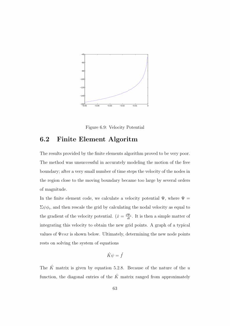
Figure 6.9: Velocity Potential

6.2 Finite Element Algoritm

The results provided by the finite elements algorithm proved to be very poor.

The method was unsuccessful in accurately modeling the motion of the free

boundary; after a very small number of time steps the velocity of the nodes in

the region close to the moving boundary became too large by several orders

of magnitude.

In the finite element code, we calculate a velocity potential Ψ, where Ψ =

Σψφi, and then rescale the grid by calculating the nodal velocity as equal to

the gradient of the velocity potential. (x = dΨi

dt. It is then a simple matter of

integrating this velocity to obtain the new grid points. A graph of a typical

values of Ψvsx is shown below. Ultimately, determining the new node points

rests on solving the system of equations

Kψ = f

The K matrix is given by equation 5.2.8. Because of the nature of the u

function, the diagonal entries of the K matrix ranged from approximately

63

40 in size, down to 0.01. This matrix was found to be ill-conditioned, which

lead to poor results for ψ.

In an effort to overcome this we take the same approach as section ??, pre-

multiplying by D−1 where the D matrix is the sum of the diagonal matrices.

This did not solve the problem of the steep gradient close to the free boundary

however, and due to time constraints we were unable to obtain any accurate

results from this method.

64

Chapter 7

conclusion

The finite difference method applied to the American Call problem produced

valuations to within −30% of the BENCH value. The undervaluing of the

option is a result of the algorithms inability to accurately resolve the true po-

sition of the moving boundary at each time step. The algorithm was found

to be unstable when applying the derivative boundary conditions directly,

hence we saught to approximate the derivative by the form of a parabola.

Although this improved stability, we believe that this reduces accuracy of

the method in determing the moving boundary, the velocity is consistently

over approximated.

The introduction of the monitor function improved results, further work is

required in analysing the effect of approximation to the boundary conditions,

there are also several further monitor functions that can be implemented. A

comparison of these methods would be the next step in our research.

We have devised a new method for the valuation of American options as free

boundary problems, transforming the equation to a Lagrangian frame, and

are also the first to introduce the Shur method for locating the free bound-

65

ary. ( To our Knowledge ) Due to time limitations we were unsuccessful in

applying the finite element algorithm to the problem. We were unable to re-

solve the problem caused by the ill-conditioned matrix when evaluating the

velocity potentials.

Concluding, further work is required in formulating the finite element ap-

proach to this problem and finding an alternative method of calculating the

velocity potential . A comparison could then be made between the accu-

racy of the finite difference method we have presented, and the finite element

method that was originally proposed.

66

Chapter 8

Reference

1 M.J.Baines A moving mesh finite element algorithm for the adaptive

solution of time-dependent partial differential equations with moving

boundaries, Applied Numerical Mathematics 54(2005)450-469

2 F.Black & M.Scholes, The pricing and Corportate Liabilities, Journal

of Political Economy, Vol. 81, 1973

3 R.L.Burden Numerical Analysis,Brooks/Cole 1997

4 L.Clewlow & C.Strickland,Implementing Derivatives Models,John Wi-

ley & Sons,1998

5 P.Garrcia-Navarro & A.Priestley, A Conservative and Shape-Preserving

Semi-Lagrangian method for the solution of Shallow Water Equations.

Numerical Analysis Report 6/93, University of Reading, 1993

6 D.J.Higham An Introduction to Financial Option Valuation. Cam-

bridge, 2004.

67

7 J.Hull Options,Futures, and Other Derivatives. Prentice-Hall Interna-

tional, 2003

8 A. Priestley, A Quasi-Conservative Version of the Semi-Lagrangian Ad-

vection Scheme. Numerical Analysis Report 2/92, University of Read-

ing, 1992.

9 K.Singh, A Comparison of Numerical Schemes for Pricing Bond Op-

tions. Msc Thesis, University of Reading, 1998

10 S.Smith, Submitted PhD thesis, University of Reading, 1996

11 G.D.Smith,Numerical Solution of Partial Differential Equations. Ox-

ford, 1985

12 I.M.Smith,Programming in Fortran 90,John Wiley & Sons, 1995

13 P.Wilmott The Mathematics of Finacial Derivatives. Cambridge 2002.

68

.1 Program 1 - pt1.f90

PROGRAM AMERICAN OPTIONS707

DOUBLE PRECISION : :K,NEGINFINITY,XN, Delt , Tf ina l , t ,B, h ,A,C, DelTau ,

Domain , Tau ,SOUT

DOUBLE PRECISION,ALLOCATABLE: :U( : ) ,UTEMP( : ) ,RHS( : ) ,Z ( : ) ,Y( : ) ,HT( : ) ,V( : ) ,

X( : ) ,U2D( : , : ) ,X2D( : , : ) ,S2D ( : , : ) ,V2D( : , : )

INTEGER: : IOS , j ,N,L , i

DOUBLE PRECISION,PARAMETER: : I r =0.03D0 , Sigma=0.5D0 ,D=0.8D0∗ I r ,KK=10.0D0

DOUBLE PRECISION,PARAMETER: : K1=2.0D0∗ I r /( Sigma ∗∗2 .0D0) ,K2=2.0D0∗( Ir−D) /(

sigma ∗∗2 .0D0)

8 PRINT∗ , ’∗∗∗∗∗∗∗∗∗∗∗∗∗∗∗∗∗∗∗∗∗∗∗∗∗∗∗∗∗∗∗∗∗∗∗∗∗∗∗∗∗∗∗∗∗ ’

PRINT∗ , ’∗ ∗ ’

PRINT∗ , ’∗ CRANK NICOLSON SOLULTION ∗ ’

PRINT∗ , ’∗ ∗ ’

PRINT∗ , ’∗ DIFFUSION EQUATION ∗ ’

PRINT∗ , ’∗ ∗ ’

PRINT∗ , ’∗ ∗ ’

PRINT∗ , ’∗∗∗∗∗∗∗∗∗∗∗∗∗∗∗∗∗∗∗∗∗∗∗∗∗∗∗∗∗∗∗∗∗∗∗∗∗∗∗∗∗∗∗∗∗ ’

16 PRINT∗

NEGINFINITY=−30.0D0

Tf ina l =((Sigma ∗∗2 .0D0) /2 . 0 ) ∗1 .0D0

Domain=NEGINFINITY

N=800

24 L=NINT( ( T f ina l /(Domain/N) ∗∗2) )

print ∗ ,L

k=(Tf ina l /L)

DelTau=(Tf ina l ) /L

B=0.0D0

32 XN=B

69

ALLOCATE(U( 0 :N) ,UTEMP(0 :N) ,RHS( 1 :N−1) ,V( 1 :N−1) ,Z ( 1 :N−1) ,Y( 1 :N−1) ,HT( 1 :N

−1)&

,X( 0 :N) ,X2D( 0 :L , 0 :N) ,U2D( 0 :L , 0 :N) ,&

S2D( 0 :L , 0 :N) ,V2D( 0 :L , 0 :N) )

U=0.0D0

UTEMP=0.0D0

40 RHS=0.0D0

V=0.0D0

Z=0.0D0

Y=0.0D0

HT=0.0D0

t =0.0D0

S2D=0.0

V2D=0.0

48

OPEN(UNIT=13,FILE=”x . dat” ,IOSTAT=IOS)

OPEN(UNIT=14,FILE=”U. dat” ,IOSTAT=IOS)

OPEN(UNIT=15,FILE=”x1 . dat” ,IOSTAT=IOS)

OPEN(UNIT=16,FILE=”U1 . dat” ,IOSTAT=IOS)



56 OPEN(UNIT=19,FILE=”x3 . dat” ,IOSTAT=IOS)















OPEN(UNIT=34,FILE=”u10 . dat” ,IOSTAT=IOS)

70


OPEN(UNIT=36,FILE=”u0 . dat” ,IOSTAT=IOS)

OPEN(UNIT=37,FILE=”S2 . dat” ,IOSTAT=IOS)

OPEN(UNIT=38,FILE=”V2 . dat” ,IOSTAT=IOS)




80 OPEN(UNIT=42,FILE=”V4 . dat” ,IOSTAT=IOS)








88 OPEN(UNIT=50,FILE=”V8 . dat” ,IOSTAT=IOS)





OPEN(UNIT=60,FILE=”x2D . dat” ,IOSTAT=IOS)

OPEN(UNIT=61,FILE=”u2D . dat” ,IOSTAT=IOS)

96

OPEN(UNIT=62,FILE=”S . dat” ,IOSTAT=IOS)

OPEN(UNIT=63,FILE=”V. dat” ,IOSTAT=IOS)



104 OPEN(UNIT=70,FILE=”SOUT. dat” ,IOSTAT=IOS)

OPEN(UNIT=71,FILE=”STIME. dat” ,IOSTAT=IOS)

IF ( IOS/=0) THEN

71

PRINT∗ , ’ Error Occured in Opening The Output File ’

112 STOP

END IF

! ∗∗∗∗∗∗∗∗∗∗∗∗∗∗∗∗∗∗∗∗∗∗∗∗∗∗∗∗∗∗∗∗∗∗∗∗∗∗∗∗∗∗∗∗∗∗∗∗∗∗∗∗∗∗

! ∗ MAIN PROGRAM ∗

! ∗ ∗

! ∗∗∗∗∗∗∗∗∗∗∗∗∗∗∗∗∗∗∗∗∗∗∗∗∗∗∗∗∗∗∗∗∗∗∗∗∗∗∗∗∗∗∗∗∗∗∗∗∗∗∗∗∗∗

120 j=0

DO i =0,N

X( i )=NEGINFINITY+(REAL( i ) /REAL(N) ) ∗(B−NEGINFINITY)

X2D( j , i )=X( i )

END DO

128

DO i =0,N

WRITE(UNIT=13,FMT=’(E12 . 6 ) ’ )X( i )

WRITE(UNIT=60,FMT= ’(4251E21 . 6 ) ’ )X2D( j , i )

END DO

136 CALL BOUNDARY CONDITIONS(N,U,X,U2D, j , L)

DO i =1 ,(N−4)

HT( i ) =0.0D0

END DO

HT(N−3)=9.0D0/4 .0D0

HT(N−2)=−1.0D0

144 HT(N−1)=4.0D0

j=0

Tau=(0.5D0∗( Sigma ∗∗2 .0D0) ) ∗ ( 1 . 0D0) ∗(REAL( j ) /REAL(L) )

h=(B−NEGINFINITY) /N

72

CALL CRANK NICOLSON(N, k ,U,RHS,B,X, t , h , DelTau ,Tau)

152

XN=XN+0.9034∗SQRT( ( 1 . 0 ∗ ( Sigma ∗∗2 .0D0) ) ∗ ( 1 . 0D0) ∗ ( 1 . 0D0/REAL(L) ) )

B=XN

DO i =0,N


END DO

160 DO i =0,N


END DO

CALL TRIDIAG SOL(N,RHS,U, k , h ,NEGINFINITY,X,U2D, j , L , S2D ,V2D, t f i n a l )

DO j =1,L

168 h=(B−NEGINFINITY) /N

Tau=((Sigma ∗∗2 .0D0) /2 .0D0) ∗ ( 1 . 0D0) ∗(REAL( j ) /REAL(L) )

CALL CRANK NICOLSON(N, k ,U,RHS,B,X, t , h , DelTau ,Tau)

CALL VEC(N,U,V, h)

CALL TRIDIAG SOL1(N,RHS,Z , k , h)

176 CALL TRIDIAG SOL2(N,V,Y, k , h)

CALL XN SOLVE(N,Y,Z ,HT,XN)

DO i =1,N−1

RHS( i )=RHS( i )−V( i ) ∗XN

184 END DO

h=(XN−NEGINFINITY) /N

73

DO i =0,N

X( i )=NEGINFINITY+(REAL( i ) /REAL(N) ) ∗(XN−NEGINFINITY)

192

X2D( j , i )=X( i )

END DO

DO i =0,N

200 WRITE(UNIT=13,FMT=’(E12 . 6 ) ’ )X( i )

WRITE(UNIT=60,FMT= ’(4251E21 . 6 ) ’ )X2D( j , i )

END DO

CALL TRIDIAG SOL(N,RHS,U, k , h ,NEGINFINITY,X,U2D, j , L , S2D ,V2D, t f i n a l )

208 B=XN

t=Tf ina l −(2.0∗Tau/sigma ∗∗2)

SOUT=(exp (XN+(1−K2) ∗ tau ) ) ∗KK

WRITE(UNIT=70,FMT=’(F12 . 6 ) ’ )SOUT

WRITE(UNIT=71,FMT=’(F12 . 6 ) ’ )Tau

216 END DO

WRITE(UNIT=15,FMT=’(F12 . 6 ) ’ ) ( (X2D( j , i ) , j =5 ,5) , i =0,N)

WRITE(UNIT=16,FMT=’(F12 . 6 ) ’ ) ( (U2D( j , i ) , j =5 ,5) , i =0,N)





224 WRITE(UNIT=21,FMT=’(F12 . 6 ) ’ ) ( (X2D( j , i ) , j =30 ,30) , i =0,N)




74





232 WRITE(UNIT=29,FMT=’(F12 . 6 ) ’ ) ( (X2D( j , i ) , j =70 ,70) , i =0,N)








240

WRITE(UNIT=37,FMT=’(F12 . 6 ) ’ ) ( (S2D( j , i ) , j =5 ,5) , i =0,N)

WRITE(UNIT=38,FMT=’(F12 . 6 ) ’ ) ( (V2D( j , i ) , j =5 ,5) , i =0,N)




248 WRITE(UNIT=42,FMT=’(F12 . 6 ) ’ ) ( (V2D( j , i ) , j =15 ,15) , i =0,N)








256 WRITE(UNIT=50,FMT=’(F12 . 6 ) ’ ) ( (V2D( j , i ) , j =50 ,50) , i =0,N)







264

75

CLOSE(UNIT=11)

CLOSE(UNIT=12)

CLOSE(UNIT=13)

CLOSE(UNIT=14)

272 CLOSE(UNIT=15)

CLOSE(UNIT=16)

CLOSE(UNIT=17)

CLOSE(UNIT=18)

CLOSE(UNIT=19)

CLOSE(UNIT=20)

CLOSE(UNIT=21)

CLOSE(UNIT=22)

280 CLOSE(UNIT=23)

CLOSE(UNIT=24)

CLOSE(UNIT=25)

CLOSE(UNIT=26)

CLOSE(UNIT=27)

CLOSE(UNIT=28)

CLOSE(UNIT=29)

CLOSE(UNIT=30)

288

CLOSE(UNIT=31)

CLOSE(UNIT=32)

CLOSE(UNIT=33)

CLOSE(UNIT=34)

CLOSE(UNIT=35)

CLOSE(UNIT=36)

CLOSE(UNIT=37)

296 CLOSE(UNIT=38)

CLOSE(UNIT=39)

CLOSE(UNIT=40)

CLOSE(UNIT=41)

CLOSE(UNIT=42)

CLOSE(UNIT=43)

CLOSE(UNIT=44)

CLOSE(UNIT=45)

304 CLOSE(UNIT=46)

CLOSE(UNIT=47)

76

CLOSE(UNIT=48)

CLOSE(UNIT=49)

CLOSE(UNIT=64)

CLOSE(UNIT=65)

312

ENDPROGRAM AMERICAN OPTIONS707

! ∗∗∗∗∗∗∗∗∗∗∗∗∗∗∗∗∗∗∗∗∗∗∗∗∗∗∗∗∗∗∗∗∗∗∗∗∗∗∗∗∗∗∗∗∗∗∗∗∗∗∗∗∗∗∗∗∗∗

! ∗ ∗

! ∗ FUNCTIONS AND SUBROUTINES ∗

! ∗ ∗

320 ! ∗∗∗∗∗∗∗∗∗∗∗∗∗∗∗∗∗∗∗∗∗∗∗∗∗∗∗∗∗∗∗∗∗∗∗∗∗∗∗∗∗∗∗∗∗∗∗∗∗∗∗∗∗∗∗∗∗∗

SUBROUTINE BOUNDARY CONDITIONS(N,U,X,U2D, j , L)

IMPLICIT NONE

INTEGER,INTENT(IN) : :N

DOUBLE PRECISION,DIMENSION( 0 :N) ,INTENT(IN) : :X

DOUBLE PRECISION,DIMENSION( 0 :N) ,INTENT(OUT) : :U

328 DOUBLE PRECISION,DIMENSION( 0 : L , 0 :N) ,INTENT(OUT) : : U2D

INTEGER: : i

INTEGER,INTENT(IN) : : j , L

DO i =0,N

U( i )=max( 1 . 0D0−EXP(X( I ) ) , 0 . 0D0)

336

U2D( j , i )=U( i )

END DO

DO i =0,N

344 WRITE(UNIT=14,FMT=’(E12 . 6 ) ’ )U( i )

77

WRITE(UNIT=61,FMT= ’(4251E21 . 6 ) ’ )U2D( j , i )

END DO

END SUBROUTINE BOUNDARY CONDITIONS

SUBROUTINE CRANK NICOLSON(N, k ,U,RHS,B,X, t , h , DelTau ,Tau)

352 IMPLICIT NONE


DOUBLE PRECISION,INTENT(IN) : : h , k ,B, t , DelTau ,Tau

DOUBLE PRECISION,DIMENSION( 0 :N) ,INTENT(IN) : : U,X

DOUBLE PRECISION,DIMENSION( 1 :N−1) ,INTENT(OUT) : :RHS

DOUBLE PRECISION,EXTERNAL: :G

DOUBLE PRECISION : : r ,TEST

INTEGER: : i

360

r=k/(h∗∗2 .0D0)

DO i =1,N−1

RHS( i )=r ∗U( i −1)+(2.0D0−2.0D0∗ r ) ∗U( i )+r ∗U( i +1)+1.0∗k∗(G(X( i ) ,Tau)+G(X(

i ) ,Tau+DelTau ) )&

+2.0D0∗(REAL( i ) /REAL(N) ) ∗ ( (U( i )−U( i −1) ) /h)∗(−B)

368 END DO

END SUBROUTINE CRANK NICOLSON

SUBROUTINE VEC(N,U,V, h)

IMPLICIT NONE


376 DOUBLE PRECISION,DIMENSION( 0 :N) ,INTENT(IN) : :U

DOUBLE PRECISION,DIMENSION( 1 :N−1) ,INTENT(OUT) : :V

DOUBLE PRECISION,INTENT(IN) : : h

INTEGER: : i

78

DO i =1,N−1

384

V( i )=−2.0D0∗(REAL( i ) /REAL(N) ) ∗(U( i )−U( i −1) ) /h

END DO

END SUBROUTINE VEC

DOUBLE PRECISION FUNCTION G(x ,Tau)

392 IMPLICIT NONE

DOUBLE PRECISION,INTENT(IN) : : x , Tau



sigma ∗∗2 .0D0)

G=(EXP(K1∗Tau) ) ∗ ( ( (K2−K1) ∗EXP(x−(K2−1.0D0) ∗Tau) )+K1)

END FUNCTION G

400

SUBROUTINE TRIDIAG SOL(N,RHS,U, k , h ,NEGINFINITY,X,U2D, j , L , S2D ,V2D, t f i n a l )

IMPLICIT NONE

DOUBLE PRECISION,INTENT(IN) : : NEGINFINITY, h , k , t f i n a l

INTEGER,INTENT(IN) : : N, j , L

DOUBLE PRECISION,DIMENSION( 0 :N) : : Alpha , s , y


DOUBLE PRECISION,DIMENSION( 1 :N−1) ,INTENT(IN) : :RHS

408 DOUBLE PRECISION,DIMENSION( 0 : L , 0 :N) ,INTENT(INOUT) : : U2D

DOUBLE PRECISION,DIMENSION( 0 : L , 0 :N) ,INTENT(INOUT) : : S2D ,V2D


DOUBLE PRECISION,DIMENSION( 0 :N) : : RES, SS

DOUBLE PRECISION : : a , b , c , Tau , r , Sv , t

INTEGER: : i , e


416 DOUBLE PRECISION,PARAMETER: : K1=(2.0D0∗ I r ) /( sigma ∗∗2 .0D0) ,K2=(2.0D0∗( Ir−D

) ) /( sigma ∗∗2 .0D0)

Alpha=0.0

s =0.0

79

y=0.0

r=k/(h∗∗2)

424 a=r

b=(2.0D0+2.0D0∗ r )

c=r

Alpha (0 )=b

S (0)=RHS(1)

Tau=(( sigma ∗∗2 .0D0) /2 .0D0) ∗ ( 1 . 0D0) ∗(REAL( j ) /REAL(L) )

432

y (0)=exp (K1∗Tau) ∗ ( 1 . 0D0−exp (X(0)−(K2−1.0D0) ∗ tau ) )

DO i =1 ,(N−3)

Alpha ( i )=b−(a∗c/Alpha ( i −1) )

S( i )=RHS( i )+(a∗S( i −1)/Alpha ( i −1) )

440

END DO

y (N−3)=S(N−3)/Alpha (N−3)

y (N−2)=(4.0D0/9 .0D0) ∗y (N−3)

y (N−1)=(1.0D0/4 .0D0) ∗y (N−2)

y (N) =0.0

448 DO i =(N−4) ,1 ,−1

y ( i )=(s ( i )+c∗y ( i +1) ) /Alpha ( i )

END DO

Sv=7.0D0

DO i =0,N

t=Tf ina l −(2.0∗Tau/sigma ∗∗2)

456 U( i )=y( i )

80

END DO

DO i =0,N

SS( i )=(exp (x ( i )+(1−K2) ∗ tau ) ) ∗KK

464

S2D( j , i )=SS( i )

RES( i )=((U( i ) ∗KK) /( exp (K1∗( tau ) ) ) )+SS( i )−KK

V2D( j , i )=RES( i )

472 U2D( j , i )=U( i )

END DO

DO i =0,N

WRITE(UNIT=62,FMT=’(E12 . 6 ) ’ ) SS( i )

480 WRITE(UNIT=63,FMT=’(E12 . 6 ) ’ )RES( i )

WRITE(UNIT=61,FMT= ’(4251E21 . 6 ) ’ )U2D( j , i )

WRITE(UNIT=14,FMT=’(E12 . 6 ) ’ )U( i )

END DO

488

END SUBROUTINE TRIDIAG SOL

SUBROUTINE TRIDIAG SOL1(N,RHS,Z , k , h)

IMPLICIT NONE


DOUBLE PRECISION,DIMENSION( 1 :N−1) : : Alpha , S , y

DOUBLE PRECISION,DIMENSION( 1 :N−1) ,INTENT(OUT) : : Z

496 DOUBLE PRECISION,DIMENSION( 1 :N−1) ,INTENT(IN) : :RHS

DOUBLE PRECISION,INTENT(IN) : : k , h

81

DOUBLE PRECISION : : a , b , c , r

INTEGER: : i

s =0.0

y=0.0

504

r=k/(h∗∗2 .0D0)

a=(r )

b=(2.0D0+2.0D0∗ r )

c=(r )

Alpha (1 )=b

S (1)=RHS(1)

512

DO i =2 ,(N−1)



520 END DO

y (N−1)=S(N−1)/Alpha (N−1)

DO i =(N−2) ,1 ,−1

y ( i )=(S( i )+c∗y ( i +1) ) /Alpha ( i )

528 END DO

DO i =1,N−1

Z( i )=y ( i )

END DO

536

82

END SUBROUTINE TRIDIAG SOL1

SUBROUTINE TRIDIAG SOL2(N,V,Y, k , h)

IMPLICIT NONE



DOUBLE PRECISION,DIMENSION( 1 :N−1) : : Alpha , s ,U

544 DOUBLE PRECISION,DIMENSION( 1 :N−1) ,INTENT(OUT) : :Y

DOUBLE PRECISION,DIMENSION( 1 :N−1) ,INTENT(IN) : :V


INTEGER: : i

s =0.0

552 Y=0.0

U=0.0

r=k/(h∗∗2 .0D0)

a=(r )

b=(2.0D0+2.0D0∗ r )

c=(r )

560

Alpha (1 )=b

S (1)=V(1)

DO i =2,N−1


S( i )=V( i )+(a∗S( i −1)/Alpha ( i −1) )

568

END DO

U(N−1)=s (N−1)/Alpha (N−1)

DO i =(N−2) ,1 ,−1

U( i )=(S( i )+c∗U( i +1) ) /Alpha ( i )

83

576

END DO

DO i =1,N−1

Y( i )=U( i )

END DO

584


SUBROUTINE XN SOLVE(N,Y, Z ,HT,XN)

IMPLICIT NONE


DOUBLE PRECISION,DIMENSION( 1 :N−1) ,INTENT(IN) : : Y, Z ,HT

592 DOUBLE PRECISION,INTENT(OUT) : :XN

DOUBLE PRECISION : : A,B

INTEGER: : i

A=0.0

B=0.0

DO i =1,N−1

600 A=A+Ht( i ) ∗Z( i )

B=B+Ht( i ) ∗Y( i )

END DO

XN=A/B

END SUBROUTINE XN SOLVE


PROGRAM movingr

DOUBLE PRECISION : :K,NEGINFINITY,XN, Delt , Tf ina l , t , h ,A,C,KN,BN, l e f t ,

domain

84

DOUBLE PRECISION,ALLOCATABLE: :U( : ) ,UTEMP( : ) ,RHS( : ) ,Z ( : ) ,Y( : ) ,HT( : ) ,V( : ) ,

X( : ) , r1 ( : ) , r2 ( : ) , r3 ( : )

INTEGER: : IOS , j ,N,L , i



sigma ∗∗2 .0D0)

8 PRINT∗ , ’∗∗∗∗∗∗∗∗∗∗∗∗∗∗∗∗∗∗∗∗∗∗∗∗∗∗∗∗∗∗∗∗∗∗∗∗∗∗∗∗∗∗∗∗∗ ’

PRINT∗ , ’∗ ∗ ’

PRINT∗ , ’∗ CRANK NICOLSON SOLULTION ∗ ’

PRINT∗ , ’∗ ∗ ’


PRINT∗ , ’∗ ∗ ’

PRINT∗ , ’∗ ∗ ’

PRINT∗ , ’∗∗∗∗∗∗∗∗∗∗∗∗∗∗∗∗∗∗∗∗∗∗∗∗∗∗∗∗∗∗∗∗∗∗∗∗∗∗∗∗∗∗∗∗∗ ’

16 PRINT∗


Tf ina l =((Sigma ∗∗2 .0D0) /2 . 0 ) ∗1 .0

Domain=NEGINFINITY

24 N=300

L=NINT( ( T f ina l /(Domain/REAL(N) ) ∗∗2) )

PRINT∗ , ( T f i na l /(Domain/REAL(N) ) ∗∗2)

k=Tf ina l /L

Le f t=−20.0D0

N=100

32 t =0.0D0

Delt =1.0D0/L

BN=0.0D0

KN=((BN−LEFT)/N∗∗2 .0D0)

85

ALLOCATE(U( 0 :N) ,UTEMP(0 :N) ,RHS( 1 :N−1) ,V( 1 :N−1) ,Z ( 1 :N−1) ,Y( 1 :N−1) ,HT( 1 :N

−1) ,X( 0 :N) ,&

40 r1 ( 1 :N−1) , r2 ( 1 :N−1) , r3 ( 1 :N−1) )

U=0.0D0

UTEMP=0.0D0

RHS=0.0D0

V=0.0D0

Z=0.0D0

Y=0.0D0

48 HT=0.0D0

t =0.0D0



56 IF ( IOS/=0) THEN

PRINT∗ , ’ Error Occured in Opening The Output File ’

STOP

END IF

! ∗∗∗∗∗∗∗∗∗∗∗∗∗∗∗∗∗∗∗∗∗∗∗∗∗∗∗∗∗∗∗∗∗∗∗∗∗∗∗∗∗∗∗∗∗∗∗∗∗∗∗∗

! ∗ ∗


64 ! ∗ ∗

! ∗∗∗∗∗∗∗∗∗∗∗∗∗∗∗∗∗∗∗∗∗∗∗∗∗∗∗∗∗∗∗∗∗∗∗∗∗∗∗∗∗∗∗∗∗∗∗∗∗∗∗∗

X(0)=LEFT

WRITE(UNIT=11,FMT=’(E12 . 6 ) ’ )X(0)

DO i =1,N−1

72 X( i )=BN−(KN∗(N−i ) ∗∗2 .0D0)


END DO

X(N)=BN

WRITE(UNIT=11,FMT=’(E12 . 6 ) ’ )X(N)

86

CALL BOUNDARY CONDITIONS(N,U,X)

80 DO i =1 ,(N−4)

HT( i ) =0.0D0

END DO

HT(N−3)=9.0D0/4 .0D0

HT(N−2)=−1.0D0

HT(N−1)=4.0D0

88 t =1.0D0

XN=BN

DO j =0,L

t=t−de l t

tau=(( sigma ∗∗2 .0D0) /2 .0D0) ∗ ( 1 . 0D0−t )

96 DO i =1 ,(N−1)

r1 ( i ) =((x ( i −1)−x ( i ) ) ∗( x ( i −1)−x ( i +1) ) )

r2 ( i ) =((x ( i )−x ( i −1) ) ∗( x ( i )−x ( i +1) ) )

r3 ( i ) =((x ( i +1)−x ( i −1) ) ∗( x ( i +1)−x ( i ) ) )

END DO

CALL CRANK NICOLSON(N, k ,U,RHS,X, t , h , de l t , r1 , r2 , r3 ,XN)

104 CALL VEC(N,U,V, h ,X)

CALL TRIDIAG SOL1(N,RHS,Z , k , r1 , r2 , r3 )

CALL TRIDIAG SOL2(N,V,Y, k , h , r1 , r2 , r3 )

CALL XN SOLVE(N,Y,Z ,HT,XN)

BN=XN

112

DO i =1,N−1

RHS( i )=RHS( i )−V( i ) ∗XN

END DO

87

KN=((BN−LEFT)/N∗∗2 .0D0)

X(0)=LEFT

120 WRITE(UNIT=11,FMT=’(E12 . 6 ) ’ )X(0)

DO i =1,N−1

X( i )=BN−(KN∗(N−i ) ∗∗2 .0D0)


END DO

X(N)=BN

WRITE(UNIT=11,FMT=’(E12 . 6 ) ’ )X(N)

128

DO i =1 ,(N−1)

r1 ( i ) =((x ( i −1)−x ( i ) ) ∗( x ( i −1)−x ( i +1) ) )

r2 ( i ) =((x ( i )−x ( i −1) ) ∗( x ( i )−x ( i +1) ) )

r3 ( i ) =((x ( i +1)−x ( i −1) ) ∗( x ( i +1)−x ( i ) ) )

END DO

136 CALL TRIDIAG SOL(N,RHS,U, t , k ,NEGINFINITY, r1 , r2 , r3 , x ) ! So lve f o r

new U

END DO

CLOSE(UNIT=11)

144 CLOSE(UNIT=12)

ENDPROGRAM movingr

! ∗∗∗∗∗∗∗∗∗∗∗∗∗∗∗∗∗∗∗∗∗∗∗∗∗∗∗∗∗∗∗∗∗∗∗∗∗∗∗∗∗∗∗∗∗∗∗∗∗∗∗∗∗∗∗∗∗∗∗∗∗∗∗∗∗

! ∗ ∗

! ∗ FUNCTIONS AND SUBROUTINES ∗

! ∗ ∗

152 ! ∗∗∗∗∗∗∗∗∗∗∗∗∗∗∗∗∗∗∗∗∗∗∗∗∗∗∗∗∗∗∗∗∗∗∗∗∗∗∗∗∗∗∗∗∗∗∗∗∗∗∗∗∗∗∗∗∗∗∗∗∗∗∗∗∗

88

SUBROUTINE BOUNDARY CONDITIONS(N,U,X)

IMPLICIT NONE




160 INTEGER: : i

DO i =0,N

U( i )=max( 1 . 0D0−EXP(X( I ) ) , 0 . 0D0)


END DO

END SUBROUTINE BOUNDARY CONDITIONS

168

SUBROUTINE CRANK NICOLSON(N, k ,U,RHS,X, t , h , de l t , r1 , r2 , r3 ,XN)

IMPLICIT NONE


DOUBLE PRECISION,INTENT(IN) : : h , k , t , de l t ,XN


DOUBLE PRECISION,DIMENSION( 1 :N−1) ,INTENT(IN) : : r1 , r2 , r3

DOUBLE PRECISION,DIMENSION( 1 :N−1) ,INTENT(OUT) : :RHS

176 DOUBLE PRECISION,EXTERNAL: :G

DOUBLE PRECISION : : TEST, tp

INTEGER: : i

tp=t−de l t

DO i =1,N−1

184 RHS( i ) =2.0∗ r1 ( i ) ∗U( i −1)+(2.0D0+2.0∗ r2 ( i ) ) ∗U( i ) +2.0∗ r3 ( i ) ∗U( i +1)+(k ) ∗(

G(X( i ) , t )+G(X( i ) , tp ) )&

+(1.0D0−(((N−i ) ∗∗2 .0D0) /N∗∗2 .0D0) ) ∗ ( (U( i )−U( i −1) ) /(x ( i )−x ( i −1) ) )∗(−XN

) ∗2 .0

!PRINT∗ , i ,RHS( i )

END DO

END SUBROUTINE CRANK NICOLSON

89

192 SUBROUTINE VEC(N,U,V, h ,X)

IMPLICIT NONE



DOUBLE PRECISION,DIMENSION( 1 :N−1) ,INTENT(OUT) : :V

DOUBLE PRECISION,INTENT(IN) : : h

INTEGER: : i

200

DO i =1,N−1

V( i )=−(2.0D0−(((N−i ) ∗∗2 .0D0) /N∗∗2 .0D0) ) ∗(U( i )−U( i −1) ) /(x ( i )−x ( i −1) )

END DO

END SUBROUTINE VEC

208 DOUBLE PRECISION FUNCTION G(x , t )

IMPLICIT NONE

DOUBLE PRECISION,INTENT(IN) : : x , t



sigma ∗∗2 .0D0)

DOUBLE PRECISION : : Tau

Tau=(0.5D0∗( Sigma ∗∗2 .0D0) ) ∗ ( 1 . 0D0−t )

216 G=(EXP(K1∗Tau) ) ∗ ( ( (K2−K1) ∗EXP(x−(K2−1.0D0) ∗Tau) )+K1)

END FUNCTION G

SUBROUTINE TRIDIAG SOL(N,RHS,U, t , k ,NEGINFINITY, r1 , r2 , r3 , x )

IMPLICIT NONE

DOUBLE PRECISION,INTENT(IN) : : NEGINFINITY, k , t


224 DOUBLE PRECISION,DIMENSION( 0 :N) : : Alpha , s , y


DOUBLE PRECISION,DIMENSION( 1 :N−1) ,INTENT(IN) : : RHS, r1 , r2 , r3

DOUBLE PRECISION,DIMENSION( 0 :N) ,INTENT(IN) : : x

DOUBLE PRECISION : : a , b , c , tau , r

90

INTEGER: : i


232 DOUBLE PRECISION,PARAMETER: : K1=(2.0D0∗ I r ) /( sigma ∗∗2 .0D0) ,K2=(2.0D0∗( Ir−D

) ) /( sigma ∗∗2 .0D0)

Alpha=0.0D0

s =0.0D0

y=0.0D0

a=2.0∗ r1 (2 )

240 b=(2.0D0−2.0∗ r2 (2 ) )

c=2.0∗ r3 (2 )

Alpha (1 )=b

S (1)=RHS(1)

tau=(( sigma ∗∗2 .0D0) /2 .0D0) ∗ ( 1 . 0D0−t )

248

DO i =2 ,(N−3)

a=2.0∗ r1 ( i )

b=(2.0D0−2.0∗ r2 ( i ) )

c=2.0D0∗ r3 ( i )



256

END DO

y (N−3)=S(N−3)/Alpha (N−3)

y (N−2)=(4.0D0/9 .0D0) ∗y (N−3)

y (N−1)=(1.0D0/4 .0D0) ∗y (N−2)

y (N) =0.0D0

264

DO i =(N−4) ,3 ,−1

y ( i )=(s ( i )+c∗y ( i +1) ) /Alpha ( i )

91

END DO

DO i =0,N

U( i )=y( i )

272 WRITE(UNIT=12,FMT=’(E12 . 6 ) ’ )U( i )

Print ∗ ,U( i )

END DO


SUBROUTINE TRIDIAG SOL1(N,RHS,Z , k , r1 , r2 , r3 )

280 IMPLICIT NONE


DOUBLE PRECISION,DIMENSION( 1 :N−1) : : Alpha , S ,Q


DOUBLE PRECISION,DIMENSION( 1 :N−1) ,INTENT(IN) : : RHS, r1 , r2 , r3

DOUBLE PRECISION,INTENT(IN) : : k


INTEGER: : i

288

s =0.0D0

a=2.0∗ r1 (1 )

b=(2.0D0−2.0∗ r2 (1 ) )

c=2.0D0∗ r3 (1 )

296

Alpha (1 )=b

S (1)=RHS(1)

DO i =2 ,(N−1)

a=2.0∗ r1 ( i )

304 b=(2.0D0−2.0∗ r2 ( i ) )

c=2.0∗ r3 ( i )

92



END DO

312 Q(N−1)=S(N−1)/Alpha (N−1)

DO i =(N−2) ,1 ,−1

Q( i )=(S( i )+c∗Q( i +1) ) /Alpha ( i )

END DO

320 DO i =1,N−1

Z( i )=Q( i )

END DO


328

SUBROUTINE TRIDIAG SOL2(N,V,Y, k , h , r1 , r2 , r3 )

IMPLICIT NONE



DOUBLE PRECISION,DIMENSION( 1 :N−1) : : Alpha , s ,D

DOUBLE PRECISION,DIMENSION( 1 :N−1) ,INTENT(OUT) : :Y

DOUBLE PRECISION,DIMENSION( 1 :N−1) ,INTENT(IN) : : V, r1 , r2 , r3

336 DOUBLE PRECISION : : a , b , c , r

INTEGER: : i

s =0.0

Y=0.0

344 a=2.0∗ r1 (1 )

93

b=2.0−2.0∗ r2 (1 )

c=2.0∗ r3 (1 )

Alpha (1 )=b

S (1)=V(1)

DO i =2,N−1

352

a=2.0∗ r1 ( i )

b=2.0D0−2.0∗ r2 ( i )

c=2.0∗ r3 ( i )


S( i )=V( i )+(a∗S( i −1)/Alpha ( i −1) )

360 END DO

D(N−1)=s (N−1)/Alpha (N−1)

DO i =(N−2) ,1 ,−1

D( i )=(S( i )+c∗D( i +1) ) /Alpha ( i )

368 END DO

DO i =1,N−1

Y( i )=D( i )

END DO

376


SUBROUTINE XN SOLVE(N,Y, Z ,HT,XN)

IMPLICIT NONE


DOUBLE PRECISION,DIMENSION( 1 :N−1) ,INTENT(IN) : : Y, Z ,HT

DOUBLE PRECISION,INTENT(OUT) : :XN

94

384 DOUBLE PRECISION : : A,B

INTEGER: : i

A=0.0D0

B=0.0D0

DO i =1,N−1

A=A+Ht( i ) ∗Z( i )

392 B=B+Ht( i ) ∗Y( i )

END DO

XN=A/B

END SUBROUTINE XN SOLVE


PROGRAM FINITE ELEMENTS V5n

DOUBLE PRECISION : : k ,NEGINFINITY, Delt , Tf ina l , t , h ,SUMG1,SUMG2, Theta1 ,

ThetaNew , tau ,SumC, Domain ,GINTERGRAL,DERIV,SUMG

DOUBLE PRECISION,ALLOCATABLE: :U( : ) ,Z ( : ) ,Y( : ) ,X( : ) ,G( : ) ,KM( : , : ) ,KP( : , : ) ,

Phi ( : ) , h Vector ( : ) ,dPdX ( : ) , Cvec ( : ) ,ThetaV ( : ) , f ( : ) ,&

W( : ) ,HT( : ) ,RHS( : ) ,M( : , : ) ,RHS1 ( : )

INTEGER: : IOS , j ,N,L , i , q

DOUBLE PRECISION,EXTERNAL: : Uprime


8 DOUBLE PRECISION,PARAMETER: : K1=2.0D0∗ I r /( Sigma ∗∗2 .0D0) ,K2=2.0D0∗( Ir−D) /(

sigma ∗∗2 .0D0)

PRINT∗ , ’∗∗∗∗∗∗∗∗∗∗∗∗∗∗∗∗∗∗∗∗∗∗∗∗∗∗∗∗∗∗∗∗∗∗∗∗∗∗∗∗∗∗∗∗∗ ’

PRINT∗ , ’∗ ∗ ’

PRINT∗ , ’∗ FINITE ELEMENT SOLULTION ∗ ’

PRINT∗ , ’∗ ∗ ’


PRINT∗ , ’∗ ∗ ’

16 PRINT∗ , ’∗ ∗ ’

PRINT∗ , ’∗∗∗∗∗∗∗∗∗∗∗∗∗∗∗∗∗∗∗∗∗∗∗∗∗∗∗∗∗∗∗∗∗∗∗∗∗∗∗∗∗∗∗∗∗ ’

95

PRINT∗


Tf ina l=(Sigma ∗∗2 .0 ) /2 .0D0

Domain=NEGINFINITY

24 N=100

L=NINT( ( T f ina l /(Domain/N) ∗∗2) )

k=(Tf ina l /L)

Delt=(T f ina l ) /L

32

t =0.0D0

GINTERGRAL=0.0

Theta1=0.0D0

B=0.0D0

f =0.0D0

40 RHS=0.0D0

ALLOCATE(U( 0 :N+1) ,G( 0 :N) ,Z ( 1 :N−1) ,Y( 1 :N) ,X( 0 :N+1) ,KM(1 :N, 0 :N+1) ,KP( 1 :N

−1 ,0:N) ,&

Phi ( 0 :N) , h vec to r ( 0 :N) ,dPdX( 0 :N) ,Cvec ( 1 :N−1)&

,ThetaV ( 0 :N) , f ( 1 :N−1) ,W( 0 :N) ,HT( 1 :N) ,RHS( 1 :N−1) ,M( 1 :N−1 ,0:N) ,RHS1( 1 :N

−1) )

SumC=0.0D0

U=0.0D0

48 Y=0.0D0

Z=0.0D0

Y=0.0D0

KM=0.0D0

KP=0.0D0

t =0.0D0

f =0.0D0

96

M=0.0D0

56



OPEN(UNIT=13,FILE=”K. dat” ,IOSTAT=IOS)

OPEN(UNIT=14,FILE=”KP. dat” ,IOSTAT=IOS)

OPEN(UNIT=15,FILE=”G. dat” ,IOSTAT=IOS)

OPEN(UNIT=16,FILE=”Phi . dat” ,IOSTAT=IOS)

64 OPEN(UNIT=17,FILE=”M. dat” ,IOSTAT=IOS)

OPEN(UNIT=18,FILE=”C. dat” ,IOSTAT=IOS)

OPEN(UNIT=19,FILE=”SumTheta . dat” ,IOSTAT=IOS)

OPEN(UNIT=20,FILE=”Y. dat” ,IOSTAT=IOS)

OPEN(UNIT=21,FILE=”dPdX. dat” ,IOSTAT=IOS)

OPEN(UNIT=22,FILE=”NewTheta . dat” ,IOSTAT=IOS)

OPEN(UNIT=23,FILE=”Z . dat” ,IOSTAT=IOS)

OPEN(UNIT=24,FILE=”W. dat” ,IOSTAT=IOS)

72 OPEN(UNIT=25,FILE=”G1. dat” ,IOSTAT=IOS)

OPEN(UNIT=26,FILE=”G2. dat” ,IOSTAT=IOS)

OPEN(UNIT=27,FILE=”Y1 . dat” ,IOSTAT=IOS)

OPEN(UNIT=28,FILE=”kk . dat” ,IOSTAT=IOS)

OPEN(UNIT=29,FILE=”Stheta . dat” ,IOSTAT=IOS)

OPEN(UNIT=30,FILE=”Yold . dat” ,IOSTAT=IOS)

OPEN(UNIT=31,FILE=”MassMul . dat” ,IOSTAT=IOS)

IF ( IOS/=0) THEN

80 PRINT∗ , ’ Error Occured in Opening The Output File ’

STOP

END IF

! ∗∗∗∗∗∗∗∗∗∗∗∗∗∗∗∗∗∗∗∗∗∗∗∗∗∗∗∗∗∗∗∗∗∗∗∗∗∗∗∗∗∗∗∗∗∗∗∗∗∗∗∗∗∗∗∗∗∗∗∗∗∗∗∗∗∗∗∗

! ∗ ∗


! ∗ ∗

88 ! ∗∗∗∗∗∗∗∗∗∗∗∗∗∗∗∗∗∗∗∗∗∗∗∗∗∗∗∗∗∗∗∗∗∗∗∗∗∗∗∗∗∗∗∗∗∗∗∗∗∗∗∗∗∗∗∗∗∗∗∗∗∗∗∗∗∗∗∗

WRITE(UNIT=28,FMT=’(E12 . 6 ) ’ ) k

DO i =0,N

97


96 WRITE(UNIT=11,FMT=’(E12 . 6 ) ’ )X( i )

END DO

CALL INITIAL DATA(N,U,X)

104

HT(1) =1.0D0

HT(2)=−1.0D0

DO i =3,N

HT( i ) =0.0D0

112

END DO

t =1.0D0

DO i =0,N−1

120 CALL Theta (X, ThetaV ,N, i , t ,U)

Theta1=Theta1+ThetaV( i )

WRITE(UNIT=19,FMT=’(E12 . 6 ) ’ ) Theta1

END DO

WRITE(UNIT=29,FMT=’(E12 . 6 ) ’ ) Theta1

128

DO q=1,1

GINTEGRAL=0.0

98

Tau=(( sigma ∗∗2 .0D0) /2 .0D0) ∗ ( 1 . 0D0) ∗(REAL( q ) /REAL(L) )

136 DO i =1,N−1

CALL Cvector (X, Cvec ,N, i , t ,U, Theta1 )

WRITE(UNIT=18,FMT=’(E12 . 6 ) ’ ) Cvec ( i )

SumC=SumC+Cvec ( i )

144 END DO

DO i =1,N−1

CALL SIMPSONS1(X,SUMG1,N, i , q , L)

CALL SIMPSONS2(X,SUMG2,N, i , q , L)

152

G( i )=SUMG1+SUMG2

WRITE(UNIT=15,FMT=’(E12 . 6 ) ’ )G( i )

END DO

G(N)=G(N−1)

160

DO i =1,N−1

CALL MASS MATRIX( i ,N,X,KM)

CALL MASS MATRIX PRIME( i ,N,X,KP,U)

END DO

168 KP(1 ,1 )=KP(1 ,1 ) /2 .0D0

RHS1(1)=U(1) ∗KM(1 ,1 )+U(2) ∗KM(1 ,2 )

99

DO j =2,N−2

176 RHS1( j )=U( j −1)∗KM( j , j −1)+U( j ) ∗KM( j , j )+U( j +1)∗KM( j , j +1)

WRITE(UNIT=31,FMT=’(E14 . 8 ) ’ )RHS1( j )

END DO

RHS1(N−1)=U(N−2)∗KM(N−1,N−2)+U(N−1)∗KM(N−1,N−1)

DO j =1,N−1

184

Y( j )=G( j )−RHS1( j )

WRITE(UNIT=27,FMT=’(E14 . 8 ) ’ )Y( j )

END DO

192 DO j =1,N−1

f ( j )=Y( j )

END DO

200 DO i =1,N

h vec to r ( i )=X( i )−X( i −1)

END DO

208 CALL TRIDIAG SOL1(N, f , Z , k ,KP)

CALL TRIDIAG SOL2(N, Cvec ,W, k ,KP)

100

CALL THETA SOLVE(N,W,Z ,HT, ThetaNew)

WRITE(UNIT=22,FMT=’(E14 . 8 ) ’ ) ThetaNew

216 DO j =1,N−1


END DO

Do i =1,N−1

224

CALL IntegrateG (X,SUMG,N, i , q , L)

GINTERGRAL=GINTERGRAL+SUMG

END DO

DERIV=−UPrime (NEGINFINITY,Tau)+GINTERGRAL

232

PRINT∗ ,THETANEW, ’New Theta ’

DO j =1,N−1

240 Y( j )=Y( j )−(THETANEW) ∗Cvec ( j )


END DO

CALL TRIDIAG SOL(N,Y,KP, Phi )

248

DO i =1,N

101

IF ( i /=N) THEN

dPdX( i ) =(((X( i )−X( i −1) ) ∗( Phi ( i )−Phi ( i −1) )+(X( i +1)−X( i ) ) ∗( Phi (

i +1)−&

Phi ( i ) ) ) ) / ( (X( i )−X( i −1) )+(X( i +1)−X( i ) ) )

256

ELSE

dPdX( i )=(Phi ( i )−Phi ( i −1) ) /(X( i )−X( i −1) )

END IF

END DO

264 dPdX(0) =0.0D0

DO i =0,N

CALL EULERS(N,X, h vector , k ,dPdX)

END DO

272 DO i =0,N

END DO

DO i =1,N−1

CALL M MATRIX( i ,N,X,M)

280

END DO

DO i =1,N−1

RHS( i )=ThetaNew∗Cvec ( i )

102

288

END DO

CALL TRIDIAG SOL3(N,M,U,RHS, tau ,NEGINFINITY)

DO i =0,N

!PRINT∗ , i ,U( i )

296 !WRITE(UNIT=12,FMT=’(E12 . 6 ) ’ )U( i )

END DO

! Theta1=ThetaNew

END DO

WRITE(UNIT=13,FMT= ’(101F14 . 8 ) ’ ) ( ( (KM( j , i ) ) , i =0,N) , j =1,N−1)

WRITE(UNIT=14,FMT= ’(101F14 . 8 ) ’ ) ( ( (KP( j , i ) ) , i =0,N) , j =1,N−1)

WRITE(UNIT=21,FMT=’(E12 . 6 ) ’ ) ( (dPdX( i ) ) , i =0,N)

304 WRITE(UNIT=17,FMT= ’(101F14 . 8 ) ’ ) ( ( (M( j , i ) ) , i =0,N) , j =1,N−1)

CLOSE(UNIT=11)

CLOSE(UNIT=12)

CLOSE(UNIT=13)

CLOSE(UNIT=14)

CLOSE(UNIT=15)

CLOSE(UNIT=16)

312 CLOSE(UNIT=17)

CLOSE(UNIT=18)

CLOSE(UNIT=19)

CLOSE(UNIT=20)

CLOSE(UNIT=21)

CLOSE(UNIT=22)

CLOSE(UNIT=23)

CLOSE(UNIT=24)

320 CLOSE(UNIT=25)

CLOSE(UNIT=26)

CLOSE(UNIT=27)

CLOSE(UNIT=28)

CLOSE(UNIT=29)

CLOSE(UNIT=30)

CLOSE(UNIT=31)

103

328 ENDPROGRAM FINITE ELEMENTS V5n

SUBROUTINE INITIAL DATA(N,U,X)

IMPLICIT NONE


DOUBLE PRECISION,DIMENSION( 0 :N+1) ,INTENT(IN) : :X

DOUBLE PRECISION,DIMENSION( 0 :N+1) ,INTENT(OUT) : :U

INTEGER: : i

336

DO i =0,N

U( i )=max( 1 . 0D0−EXP(X( I ) ) , 0 . 0D0)


END DO

344

END SUBROUTINE INITIAL DATA

SUBROUTINE IntegrateG (X,SUMG,N, i , q , L)

IMPLICIT NONE

INTEGER,INTENT(IN) : : N, i , q , L


DOUBLE PRECISION,INTENT(OUT) : :SUMG

352 DOUBLE PRECISION : : h , XI0 , XI2 , XI1 , a , b , XI ,SUM,Tau

DOUBLE PRECISION,EXTERNAL: :GF

DOUBLE PRECISION,PARAMETER: : Sigma=0.4D0

INTEGER: : k ,M

Tau=((Sigma ∗∗2 .0D0) /2 .0D0) ∗ ( 0 . 5D0) ∗(REAL( q ) /REAL(L) )

SUMG=0.0

360

M=INT(N∗200)

a=X( i −1)

b=X( i )

h=ABS( (X( i )−X( i −1) ) ) /M

104

XI0=GF(b ,Tau)+GF(a ,Tau)

368 XI1=0.0D0

XI2=0.0D0

DO k=1,M−1

XI=a+k∗h

IF (MOD(k , i n t (2 ) ) /=0) THEN

376

XI2=XI2+GF(XI ,Tau)

ELSE

XI1=XI1+GF(XI ,Tau)

END IF

END DO

384 SUMG=h∗(XI0+2.0D0∗XI2+4.0∗XI1 ) /3 .0D0

END SUBROUTINE IntegrateG

SUBROUTINE SIMPSONS1(X,SUMG1,N, i , q , L)

392 IMPLICIT NONE



DOUBLE PRECISION,INTENT(OUT) : : SUMG1

DOUBLE PRECISION : : h , XI0 , XI2 , XI1 , a , b , XI ,SUM,Tau


DOUBLE PRECISION,PARAMETER: : Sigma=0.4D0

INTEGER: : k ,M

400


M=N∗200

a=X( i −1)

105

b=X( i )

h=ABS( (X( i )−X( i −1) ) ) /M

408

XI0=(b−X( i −1) ) ∗GF(b , Tau)+(a−X( i −1) ) ∗GF(a ,Tau)

XI1=0.0D0

XI2=0.0D0

DO k=1,M−1

XI=a+k∗h

416

IF (MOD(k , i n t (2 ) ) /=0) THEN

XI2=XI2+(XI−X( i −1) ) ∗GF(XI ,Tau)

ELSE

XI1=XI1+(XI−X( i −1) ) ∗GF(XI , Tau)

END IF

424 END DO

SUM=h∗(XI0+2.0D0∗XI2+4.0∗XI1 ) /3 .0D0

SUMG1=SUM∗ ( 1 . 0D0/(X( i )−X( i −1) ) )

WRITE(UNIT=25,FMT=’(E12 . 6 ) ’ )SUMG1

432 END SUBROUTINE SIMPSONS1

SUBROUTINE SIMPSONS2(X,SUMG2,N, i , q , L)

IMPLICIT NONE



DOUBLE PRECISION,INTENT(OUT) : : SUMG2

DOUBLE PRECISION : : h , XI0 , XI2 , XI1 , a , XI , b ,SUM,Tau

440 DOUBLE PRECISION,PARAMETER: : Sigma=0.4


INTEGER: : k ,M

106


a=X( i )

b=X( i +1)

448 M=N∗200

h=ABS( (X( i +1)−X( i ) ) ) /M

XI0=(X( i +1)−a ) ∗GF(a , Tau)+(X( i +1)−b) ∗GF(b ,Tau)

XI1=0.0D0

XI2=0.0D0

DO k=1,M−1

456

XI=a+k∗h

IF (MOD(k , i n t (2 ) ) /=0) THEN

XI2=XI2+(X( i +1)−XI) ∗GF(XI ,Tau)

ELSE

XI1=XI1+(X( i +1)−XI) ∗GF(XI , Tau)

464

END IF

END DO

SUM=h∗(XI0+2.0D0∗XI2+4.0∗XI1 ) /3 .0D0

SUMG2=SUM∗ ( 1 . 0D0/(X( i +1)−X( i ) ) )

WRITE(UNIT=26,FMT=’(E12 . 6 ) ’ )SUMG2

472

END SUBROUTINE SIMPSONS2

DOUBLE PRECISION FUNCTION GF(x , tau )

480 IMPLICIT NONE

DOUBLE PRECISION,INTENT(IN) : : x , tau


107


sigma ∗∗2 .0D0)

488 GF=(EXP(K1∗Tau) ) ∗ ( ( (K2−K1) ∗EXP(x−(K2−1.0D0) ∗Tau) )+K1)

END FUNCTION GF

DOUBLE PRECISION FUNCTION UPrime (x , Tau)

IMPLICIT NONE

496 DOUBLE PRECISION,INTENT(IN) : : x , Tau



sigma ∗∗2 .0D0)

UPrime=−exp (K1∗Tau) ∗( exp (x−(K2−1)∗Tau) )

504

END FUNCTION Uprime

SUBROUTINE MASS MATRIX( i ,N,X,KM)

IMPLICIT NONE

512 INTEGER,INTENT(IN) : : N, i


DOUBLE PRECISION,DIMENSION( 1 :N, 0 :N+1) ,INTENT(INOUT) : :KM

DOUBLE PRECISION : : SUM1,SUM2,SUM3,SUM4,SUM

DOUBLE PRECISION,EXTERNAL: : func

DOUBLE PRECISION : : a , b , h , XI , XI1 , XI2 , XI0

INTEGER: : k ,M

108

520 a=X( i −1)

b=X( i )

M=INT(N∗200)

h=ABS( (X( i )−X( i −1) ) ) /M

XI0=func ( a )+func (b)

XI1=0.0D0

528 XI2=0.0D0

XI=0.0D0

DO k=1,M−1

XI=a+k∗h

IF (MOD(k , i n t (2 ) ) /=0) THEN

536

XI2=XI2+func (XI )

ELSE

XI1=XI1+func (XI )

END IF

END DO

544 SUM=h ∗ ( ( XI0+2.0D0∗XI2+4.0∗XI1 ) /3 .0D0)

SUM1=((1.0D0/(X( i )−X( i −1) ) ) )

a=X( i )

b=X( i +1)

552 h=ABS( (X( i +1)−X( i ) ) ) /M


XI1=0.0D0

XI2=0.0D0

XI=0.0

109

DO k=1,M−1

560

XI=a+k∗h

IF (MOD(k , i n t (2 ) ) /=0) THEN

XI2=XI2+func (XI )

ELSE

XI1=XI1+func (XI )

568

END IF

END DO

SUM=(h) ∗(XI0+2.0D0∗XI2+4.0∗XI1 ) /3 .0D0

SUM2=(1.0D0/(X( i +1)−X( i ) ) )

576 KM( i , i )=SUM1+SUM2

a=X( i )

b=X( i +1)

h=ABS( (X( i +1)−X( i ) ) ) /M


584 XI1=0.0D0

XI2=0.0D0

XI=0.0

DO k=1,M−1

XI=a+k∗h

592 IF (MOD(k , i n t (2 ) ) /=0) THEN

XI2=XI2+func (XI )

ELSE

XI1=XI1+func (XI )

110

END IF

600 END DO

SUM=h∗(XI0+2.0D0∗XI2+4.0∗XI1 ) /3 .0D0

SUM3=−1.0∗((1.0D0/(X( i +1)−X( i ) ) ∗∗2) ) ∗SUM

KM( i , i +1)=−1.0D0∗ ( 1 . 0D0/(X( i +1)−X( i ) ) )

a=X( i −1)

b=X( i )

608

h=ABS( (X( i )−X( i −1) ) ) /M


XI1=0.0D0

XI2=0.0D0

XI=0.0D0

616 DO k=1,M−1

XI=a+k∗h

IF (MOD(k , i n t (2 ) ) /=0) THEN

XI2=XI2+func (XI )

ELSE

624 XI1=XI1+func (XI )

END IF

END DO

SUM=h∗(XI0+2.0D0∗XI2+4.0∗XI1 ) /3 .0D0

SUM4=−1.0D0∗ ( ( 1 . 0D0/(X( i )−X( i −1) ) ) ∗∗2) ∗SUM

632 KM( i , i −1)=−1.0D0∗ ( 1 . 0D0/(X( i )−X( i −1) ) )

END SUBROUTINE MASS MATRIX

111

DOUBLE PRECISION FUNCTION func (x )

IMPLICIT NONE

640 DOUBLE PRECISION,INTENT(IN) : : x

func =1.0D0

END FUNCTION func

DOUBLE PRECISION FUNCTION UINTER1(UN,UM,UP, Xin , i , a , b )

IMPLICIT NONE

648 INTEGER,INTENT(IN) : : i

DOUBLE PRECISION,INTENT(IN) : :UN,UM,UP

DOUBLE PRECISION,INTENT(IN) : : a , b

DOUBLE PRECISION,INTENT(IN) : : Xin

UINTER1=UM∗(Xin−a ) /(b−a )+UN∗ ( ( b−Xin ) /(b−a ) )

END FUNCTION UINTER1

656

DOUBLE PRECISION FUNCTION UINTER2(UN,UM,UP, Xin , i , a , b )

IMPLICIT NONE

INTEGER,INTENT(IN) : : i

DOUBLE PRECISION,INTENT(IN) : :UN,UM,UP

DOUBLE PRECISION,INTENT(IN) : : a , b


664 UINTER2=UM∗(b−Xin ) /(b−a )+UP∗(Xin−a ) /(b−a )

END FUNCTION UINTER2

DOUBLE PRECISION FUNCTION UINTER(UP,UM, Xin , i , a , b )

IMPLICIT NONE

INTEGER,INTENT(IN) : : i

DOUBLE PRECISION,INTENT(IN) : :UP,UM

672 DOUBLE PRECISION,INTENT(IN) : : a , b


UINTER=UM∗(b−Xin ) /(b−a )+UP∗ ( ( Xin−a ) /(b−a ) )

112

END FUNCTION UINTER

SUBROUTINE MASS MATRIX PRIME( i ,N,X,KP,U)

680 IMPLICIT NONE

INTEGER,INTENT(IN) : : N, i


DOUBLE PRECISION,DIMENSION( 0 :N) ,INTENT(IN) : :U

DOUBLE PRECISION,DIMENSION( 1 :N−1 ,0:N) ,INTENT(INOUT) : :KP

DOUBLE PRECISION : : SUM1,SUM2,SUM3,SUM4, e , f , g

DOUBLE PRECISION : : a , b , h , XI , XI1 , XI2 , XI0 ,UN,UM,UP,TEST,SUM

688 DOUBLE PRECISION,EXTERNAL: : UINTER1,UINTER2

INTEGER: : k ,M

UN=U( i −1)

UM=U( i )

UP=U( i +1)

a=X( i −1)

696 b=X( i )

M=N∗200

h=ABS( (X( i )−X( i −1) ) ) /M

XI0=UINTER1(UN,UM,UP, a , i , a , b )+UINTER1(UN,UM,UP, b , i , a , b )

XI1=0.0D0

XI2=0.0D0

XI=0.0

704

DO k=1,M−1

XI=a+k∗h

IF (MOD(k , i n t (2 ) ) /=0) THEN

XI2=XI2+UINTER1(UN,UM,UP, XI , i , a , b )

712 ELSE


113

END IF

END DO

SUM=(h) ∗(XI0+2.0D0∗XI2+4.0∗XI1 ) /3 .0D0

SUM1=SUM∗ ( ( 1 . 0D0/(X( i )−X( i −1) ) ) ∗∗2 .0D0)

720

b=X( i +1)

a=X( i )

h=(X( i +1)−X( i ) ) /M


XI1=0.0D0

XI2=0.0D0

728 XI=0.0D0

DO k=1,M−1

XI=a+k∗h

IF (MOD(k , i n t (2 ) ) /=0) THEN

736 XI2=XI2+UINTER2(UN,UM,UP, XI , i , a , b )

ELSE


END IF

END DO

744 SUM=(h) ∗(XI0+2.0D0∗XI2+4.0∗XI1 ) /3 .0D0

SUM2=SUM∗ ( ( 1 . 0D0/(X( i +1)−X( i ) ) ) ∗∗2 .0D0)

KP( i , i )=SUM1+SUM2

f=KP( i , i )

b=X( i +1)

a=X( i )

752

h=ABS( (X( i +1)−X( i ) ) ) /M

114


XI1=0.0D0

XI2=0.0D0

XI=0.0D0

760 DO k=1,M−1

XI=a+k∗h

IF (MOD(k , i n t (2 ) ) /=0) THEN


ELSE

768 XI1=XI1+UINTER2(UN,UM,UP, XI , i , a , b )

END IF

END DO

SUM=h∗(XI0+2.0D0∗XI2+4.0∗XI1 ) /3 .0D0

SUM3=SUM∗(−1.0D0) ∗ ( ( 1 . 0D0/(X( i +1)−X( i ) ) ) ∗∗2 .0D0)

776 KP( i , i +1)=SUM3

g=KP( i , i +1)

b=X( i )

a=X( i −1)

h=ABS( (X( i )−X( i −1) ) ) /M

784 XI0=UINTER1(UN,UM,UP, a , i , a , b )+UINTER1(UN,UM,UP, b , i , a , b )

XI1=0.0D0

XI2=0.0D0

XI=0.0D0

DO k=1,M−1

XI=a+k∗h

792

115

IF (MOD(k , i n t (2 ) ) /=0) THEN


TEST=UINTER1(UN,UM,UP, XI , i , a , b )

ELSE


800

END IF

END DO

SUM=h∗(XI0+2.0D0∗XI2+4.0∗XI1 ) /3 .0D0

SUM4=SUM∗((−1.0D0) ∗ ( ( 1 . 0D0/(X( i )−X( i −1) ) ) ∗∗2 .0D0) )

KP( i , i −1)=SUM4

808 e=KP( i , i −1)

END SUBROUTINE MASS MATRIX PRIME

SUBROUTINE TRIDIAG SOL(N,Y,KP, Phi )

IMPLICIT NONE

816 INTEGER,INTENT(IN) : :N

DOUBLE PRECISION,DIMENSION( 1 :N) : : Alpha , S ,C

DOUBLE PRECISION,DIMENSION( 0 :N) ,INTENT(INOUT) : : Phi

DOUBLE PRECISION,DIMENSION( 1 :N−1) ,INTENT(IN) : :Y

DOUBLE PRECISION,DIMENSION( 0 :N) : : Z

DOUBLE PRECISION,DIMENSION( 1 :N−1 ,0:N) ,INTENT(IN) : :KP

DOUBLE PRECISION : : a , b

INTEGER: : i

824

S=0.0D0

a=−KP(1 ,0 )

b=KP(1 ,1 )

c (1 )=−KP(1 ,2 )

Alpha (1 )=b

116

832 S (1)=Y(1)

DO i =2 ,(N−1)

a=−KP( i , i −1)

b=KP( i , i )

c ( i )=−KP( i , i +1)

840

Alpha ( i )=b−(a∗c ( i −1)/Alpha ( i −1) )

S( i )=Y( i )+(a∗S( i −1)/Alpha ( i −1) )

END DO

Z(N−1)=S(N−1)/Alpha (N−1)

848 DO i =(N−2) ,1 ,−1

Z( i )=(S( i )+c ( i ) ∗Z( i +1) ) /Alpha ( i )

END DO

Z(N)=Z(N−1)

Z(0 )=Z(1)

856 DO i =0,N

Phi ( i )=Z( i )

WRITE(UNIT=16,FMT=’(E12 . 6 ) ’ ) Phi ( i )

864

END DO


SUBROUTINE EULERS(N,X, h vector , k ,dPdX)

117

IMPLICIT NONE

872 INTEGER,INTENT(IN) : :N

DOUBLE PRECISION,DIMENSION( 0 :N) ,INTENT(INOUT) : :X

DOUBLE PRECISION,DIMENSION( 0 :N) ,INTENT(IN) : : dPdX


DOUBLE PRECISION,DIMENSION(1 ,N−1) ,INTENT(IN) : : h vec to r

INTEGER: : i

DO i =0,N

880

X( i )=X( i )+k∗dPdX( i )

END DO

END SUBROUTINE EULERS

888

SUBROUTINE Cvector (X, Cvec ,N, i , t ,U, Theta1 )

IMPLICIT NONE


DOUBLE PRECISION,INTENT(IN) : : t

DOUBLE PRECISION,INTENT(IN) : : Theta1



896 DOUBLE PRECISION,DIMENSION( 1 :N−1) ,INTENT(INOUT) : : Cvec

DOUBLE PRECISION,EXTERNAL: : UINTER1,UINTER2

DOUBLE PRECISION : : h , XI0 , XI2 , XI1 , a , XI ,SUMC1,SUMC2,UN,UM,UP, b ,SUM,TEST

INTEGER: : k ,M

M=N∗300

a=X( i −1)

b=X( i )

904 h=ABS( (X( i )−X( i −1) ) ) /M

UN=U( i −1)

UM=U( i )

UP=U( i +1)

118

XI0=(a−X( i −1) ) ∗UINTER1(UN,UM,UP, a , i , a , b )+(b−X( i −1) ) ∗UINTER1(UN,UM,UP

, b , i , a , b )

912 XI1=0.0D0

XI2=0.0D0

DO k=1,M−1

XI=a+k∗h

IF (MOD(k , i n t (2 ) ) /=0) THEN

920

XI2=XI2+(XI−X( i −1) ) ∗UINTER1(UN,UM,UP, XI , i , a , b )

ELSE

XI1=XI1+(XI−X( i −1) ) ∗UINTER1(UN,UM,UP, XI , i , a , b )

END IF

END DO

928

SUM=h∗(XI0+2.0D0∗XI2+4.0∗XI1 ) /3 .0D0

SUMC1=(1.0D0/(X( i )−X( i −1) ) ) ∗SUM

b=X( i +1)

a=X( i )

936

h=ABS( (X( i +1)−X( i ) ) ) /M

XI0=(X( i +1)−a ) ∗UINTER2(UN,UM,UP, a , i , a , b )+(X( i +1)−b) ∗UINTER2(UN,UM,UP

, b , i , a , b )

XI1=0.0D0

XI2=0.0D0

944

DO k=1,M−1

119

XI=a+k∗h

IF (MOD(k , i n t (2 ) ) /=0) THEN

XI2=XI2+(X( i +1)−XI) ∗UINTER2(UN,UM,UP, XI , i , a , b )

952 ELSE

XI1=XI1+(X( i +1)−XI) ∗UINTER2(UN,UM,UP, XI , i , a , b )

TEST=UINTER2(UN,UM,UP, XI , i , a , b )

END IF

END DO

960 SUM=h∗(XI0+2.0D0∗XI2+4.0∗XI1 ) /3 .0D0

SUMC2=(1.0D0/(X( i +1)−X( i ) ) ) ∗SUM

Cvec ( i )=(SUMC1+SUMC2) /Theta1

END SUBROUTINE Cvector

968

SUBROUTINE Theta (X, ThetaV ,N, i , t ,U)

IMPLICIT NONE


DOUBLE PRECISION,INTENT(IN) : : t



976 DOUBLE PRECISION,DIMENSION( 0 :N) ,INTENT(INOUT) : : ThetaV

DOUBLE PRECISION,EXTERNAL: : UINTER

DOUBLE PRECISION : : h , XI0 , XI2 , XI1 , a , XI ,SUMC1,UP,UM, b , t e s t

INTEGER: : k ,M

M=(N∗3000)

a=X( i )

b=X( i +1)

984 h=ABS( (X( i +1)−X( i ) ) ) /M

120

UP=U( i +1)

UM=U( i )

XI0=UINTER(UP,UM, a , i , a , b )+UINTER(UP,UM, b , i , a , b )

992 XI1=0.0D0

XI2=0.0D0

DO k=1,M−1

XI=a+k∗h

IF (MOD(k , i n t (2 ) ) /=0) THEN

1000

XI2=XI2+UINTER(UP,UM, XI , i , a , b )

ELSE

XI1=XI1+UINTER(UP,UM, XI , i , a , b )

END IF

END DO

1008

SUMC1=h∗(XI0+2.0D0∗XI2+4.0∗XI1 ) /3 .0D0

ThetaV( i )=SUMC1

END SUBROUTINE Theta

SUBROUTINE TRIDIAG SOL1(N, f , Z , k ,KP)

1016 IMPLICIT NONE


DOUBLE PRECISION,DIMENSION( 1 :N−1) : : Alpha , S , y ,C


DOUBLE PRECISION,DIMENSION( 1 :N−1) ,INTENT(IN) : : f



DOUBLE PRECISION : : a , b , r

1024 INTEGER: : i

121

s =0.0D0

y=0.0D0

1032 a=−KP(1 ,0 )

b=KP(1 ,1 )

c (1 )=−KP(1 ,2 )

Alpha (1 )=b

S (1)=f (1 )

1040 DO i =2 ,(N−1)

a=−KP( i , i −1)

b=KP( i , i )

c ( i )=−KP( i , i +1)


1048 S( i )=f ( i )+(a∗S( i −1)/Alpha ( i −1) )

END DO

y (N−1)=S(N−1)/Alpha (N−1)

DO i =(N−2) ,1 ,−1

1056 y ( i )=(S( i )+c ( i ) ∗y ( i +1) ) /Alpha ( i )

END DO

DO i =1,N−1

Z( i )=y ( i )

WRITE(UNIT=23,FMT=’(E12 . 6 ) ’ )Z( i )

122

1064 END DO


SUBROUTINE TRIDIAG SOL2(N, Cvec ,W, k ,KP)

IMPLICIT NONE


1072 DOUBLE PRECISION,INTENT(IN) : : k

DOUBLE PRECISION,DIMENSION( 1 :N−1) : : Alpha , s ,U,C

DOUBLE PRECISION,DIMENSION( 1 :N−1) ,INTENT(OUT) : :W


DOUBLE PRECISION,DIMENSION( 1 :N−1) ,INTENT(IN) : : Cvec

DOUBLE PRECISION : : a , b , r

INTEGER: : i

1080

s =0.0D0

W=0.0D0

U=0.0D0

1088 a=−KP(1 ,0 )

b=KP(1 ,1 )

c (1 )=−KP(1 ,2 )

Alpha (1 )=b

S (1)=(Cvec (1 ) /k )

DO i =2,N−1

1096

a=−KP( i , i −1)

b=KP( i , i )

c ( i )=−KP( i , i +1)


S( i )=(Cvec ( i ) /k )+(a∗S( i −1)/Alpha ( i −1) )

123

1104 END DO

U(N−1)=s (N−1)/Alpha (N−1)

DO i =(N−2) ,1 ,−1

U( i )=(S( i )+C( i ) ∗U( i +1) ) /Alpha ( i )

1112 END DO

DO i =1,N−1

W( i )=U( i )

WRITE(UNIT=24,FMT=’(E12 . 6 ) ’ )W( i )

END DO

1120


SUBROUTINE THETA SOLVE(N,W,Z ,HT, ThetaNew)

IMPLICIT NONE


DOUBLE PRECISION,DIMENSION( 1 :N−1) ,INTENT(IN) : :W,Z ,HT

DOUBLE PRECISION,INTENT(OUT) : : ThetaNew

1128 DOUBLE PRECISION : : A,B

INTEGER: : i

A=0.0D0

B=0.0D0

DO i =1,N−1

A=A+Ht( i ) ∗Z( i )

1136 B=B+Ht( i ) ∗W( i )

END DO

ThetaNew=A/B

124

END SUBROUTINE THETA SOLVE

1144 SUBROUTINE TRIDIAG SOL3(N,M,U,RHS, tau ,NEGINFINITY)

IMPLICIT NONE


DOUBLE PRECISION,DIMENSION( 1 :N) : : Alpha , S ,C

DOUBLE PRECISION,DIMENSION( 0 :N) ,INTENT(INOUT) : :U

DOUBLE PRECISION,DIMENSION( 1 :N−1) ,INTENT(IN) : :RHS

DOUBLE PRECISION,DIMENSION( 1 :N−1) : : Z

DOUBLE PRECISION,INTENT(IN) : : tau ,NEGINFINITY

1152 DOUBLE PRECISION,DIMENSION( 1 :N−1 ,0:N) ,INTENT(IN) : :M



sigma ∗∗2 .0D0)

DOUBLE PRECISION : : a , b

INTEGER: : i

1160 S=0.0D0

a=M(1 ,0 )

b=M(1 ,1 )

c (1 )=M(1 ,2 )

Alpha=0.0D0

Alpha (1 )=b

S (1)=RHS(1)

1168

DO i =2 ,(N−1)

a=M( i , i −1)

b=M( i , i )

c ( i )=M( i , i +1)

1176 Alpha ( i )=b−(a∗c ( i −1)/Alpha ( i −1) )


END DO

125

Z(N−1)=S(N−1)/Alpha (N−1)

DO i =(N−2) ,1 ,−1

1184

Z( i )=(S( i )+c ( i ) ∗Z( i +1) ) /Alpha ( i )

END DO

DO i =1,N−1

U( i )=Z( i )

1192

END DO

U(0)=exp (K1∗ tau ) ∗ ( 1 . 0D0−exp (NEGINFINITY−(K2−1.0D0) ∗ tau ) )

U(N) =0.0


1200

SUBROUTINE M MATRIX( i ,N,X,M)

IMPLICIT NONE



DOUBLE PRECISION,DIMENSION( 1 :N−1 ,0:N) ,INTENT(INOUT) : :M

DOUBLE PRECISION : : SUM1,SUM2,SUM3,SUM4,SUM

1208 DOUBLE PRECISION,EXTERNAL: : func

DOUBLE PRECISION : : a , b , h , XI , XI1 , XI2 , XI0

INTEGER: : k ,MI

a=X( i −1)

b=X( i )

MI=in t (N∗200)

h=ABS( (X( i )−X( i −1) ) ) /MI

1216

XI0=(b−a ) ∗∗2+(a−a ) ∗∗2

XI1=0.0D0

126

XI2=0.0D0

XI=0.0

DO k=1,MI−1

1224 XI=a+k∗h

IF (MOD(k , i n t (2 ) ) /=0) THEN

XI2=XI2+((XI−a ) ∗∗2)

ELSE

XI1=XI1+((XI−a ) ∗∗2)

1232 END IF

END DO

SUM=(h) ∗(XI0+2.0D0∗XI2+4.0∗XI1 ) /3 .0D0

SUM1=(((b∗∗3−a ∗∗3) /3)+b∗( a ∗∗2)−a ∗(b∗∗2) ) / ( (X( i )−X( i −1) ) ∗∗2)

a=X( i )

b=X( i +1)

1240

h=ABS( (X( i +1)−X( i ) ) ) /MI

XI0=(b−b) ∗∗2+(b−a ) ∗∗2

XI1=0.0D0

XI2=0.0D0

XI=0.0

1248 DO k=1,MI−1

XI=a+k∗h

IF (MOD(k , i n t (2 ) ) /=0) THEN

XI2=XI2+((b−XI) ∗∗2)

ELSE

1256 XI1=XI1+((b−XI) ∗∗2)

127

END IF

END DO

SUM=(h) ∗(XI0+2.0D0∗XI2+4.0∗XI1 ) /3 .0D0

SUM2=(((b∗∗3−a ∗∗3) /3 .0D0) +((a ∗∗2) ∗b−a ∗(b∗∗2) ) ) / ( (X( i +1)−X( i ) ) ∗∗2)

1264

M( i , i )=SUM1+SUM2

a=X( i )

b=X( i +1)

1272 h=ABS( (X( i +1)−X( i ) ) ) /MI

XI0=(b−b) ∗(b−a )+(b−a ) ∗( a−a )

XI1=0.0D0

XI2=0.0D0

XI=0.0

DO k=1,MI−1

1280

XI=a+k∗h

IF (MOD(k , i n t (2 ) ) /=0) THEN

XI2=XI2+((b−XI) ∗(XI−a ) )

ELSE

XI1=XI1+((b−XI) ∗(XI−a ) )

1288

END IF

END DO

SUM=h∗(XI0+2.0D0∗XI2+4.0∗XI1 ) /3 .0D0

SUM3=SUM∗ ( ( 1 . 0D0/(X( i +1)−X( i ) ) ) ∗∗2)

M( i , i +1)=−1.0D0∗ ( ( ( b∗∗3−a ∗∗3) /6 .0D0) +((a ∗∗2) ∗b−a ∗(b∗∗2) ) /2 .0D0) /( (X(

i +1)−X( i ) ) ∗∗2)

128

1296

a=X( i −1)

b=X( i )

h=ABS( (X( i )−X( i −1) ) ) /MI

XI0=(b−a ) ∗( a−a )+(b−b) ∗(b−a )

1304 XI1=0.0D0

XI2=0.0D0

XI=0.0

DO k=1,MI−1

XI=a+k∗h

1312 IF (MOD(k , i n t (2 ) ) /=0) THEN

XI2=XI2+((b−XI) ∗(XI−a ) )

ELSE

XI1=XI1+((b−XI) ∗(XI−a ) )

END IF

1320 END DO

SUM=h∗(XI0+2.0D0∗XI2+4.0∗XI1 ) /3 .0D0

SUM4=((1.0D0/(X( i )−X( i −1) ) ) ∗∗2) ∗SUM

M( i , i −1)=−1.0D0∗ ( ( ( b∗∗3−a ∗∗3) /6 .0D0) +((a ∗∗2) ∗b−a ∗(b∗∗2) ) /2 .0D0) /( (X(

i +1)−X( i ) ) ∗∗2)

END SUBROUTINE M MATRIX

129

Numerical Methods For American Options · 2008-04-14 · Figure 1.1: Payoﬀ Diagram for a European...

Documents

Transcript of Numerical Methods For American Options · 2008-04-14 · Figure 1.1: Payoﬀ Diagram for a European...