NUMERICAL CFD ANALYSIS IN A RADIAL DECANTER

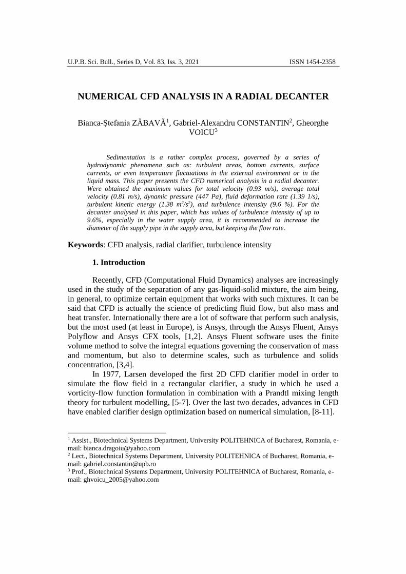
U.P.B. Sci. Bull., Series D, Vol. 83, Iss. 3, 2021 ISSN 1454-2358

NUMERICAL CFD ANALYSIS IN A RADIAL DECANTER

Bianca-Ștefania ZĂBAVĂ1, Gabriel-Alexandru CONSTANTIN2, Gheorghe

VOICU3

Sedimentation is a rather complex process, governed by a series of

hydrodynamic phenomena such as: turbulent areas, bottom currents, surface

currents, or even temperature fluctuations in the external environment or in the

liquid mass. This paper presents the CFD numerical analysis in a radial decanter.

Were obtained the maximum values for total velocity (0.93 m/s), average total

velocity (0.81 m/s), dynamic pressure (447 Pa), fluid deformation rate (1.39 1/s),

turbulent kinetic energy (1.38 m2/s2), and turbulence intensity (9.6 %). For the

decanter analysed in this paper, which has values of turbulence intensity of up to

9.6%, especially in the water supply area, it is recommended to increase the

diameter of the supply pipe in the supply area, but keeping the flow rate.

Keywords: CFD analysis, radial clarifier, turbulence intensity

1. Introduction

Recently, CFD (Computational Fluid Dynamics) analyses are increasingly

used in the study of the separation of any gas-liquid-solid mixture, the aim being,

in general, to optimize certain equipment that works with such mixtures. It can be

said that CFD is actually the science of predicting fluid flow, but also mass and

heat transfer. Internationally there are a lot of software that perform such analysis,

but the most used (at least in Europe), is Ansys, through the Ansys Fluent, Ansys

Polyflow and Ansys CFX tools, [1,2]. Ansys Fluent software uses the finite

volume method to solve the integral equations governing the conservation of mass

and momentum, but also to determine scales, such as turbulence and solids

concentration, [3,4].

In 1977, Larsen developed the first 2D CFD clarifier model in order to

simulate the flow field in a rectangular clarifier, a study in which he used a

vorticity-flow function formulation in combination with a Prandtl mixing length

theory for turbulent modelling, [5-7]. Over the last two decades, advances in CFD

have enabled clarifier design optimization based on numerical simulation, [8-11].

1 Assist., Biotechnical Systems Department, University POLITEHNICA of Bucharest, Romania, e-

mail: [email protected] 2 Lect., Biotechnical Systems Department, University POLITEHNICA of Bucharest, Romania, e-

mail: [email protected] 3 Prof., Biotechnical Systems Department, University POLITEHNICA of Bucharest, Romania, e-

mail: [email protected]

266 Bianca-Ștefania Zăbavă, Gabriel-Alexandru Constantin, Gheorghe Voicu

The aim of this study was to simulate the flow of a liquid-solid mixture

inside a radial clarifier, in the feeding area. It should be mentioned that a 2D study

of the flow analysis was done.

In figure 1 a methodology for analysing the flow of the liquid-solid

mixture is presented.

Fig. 1. Methodology for analysing the flow of the mixture through the radial decanter

The mathematical equations governing this study are presented below, [12-

15].

The continuity equation has the form: 𝜕𝜌

𝜕𝑡+ ∇ ∙ (𝜌�⃗� ) = 0 (1)

Momentum equation can be calculated with: 𝜕(𝜌�⃗⃗� )

𝜕𝑡+ ∇ ∙ (𝜌�⃗� �⃗� ) = −∇𝑃 + 𝜌𝑔 + 𝑓 (2)

where t is time, ρ is the fluid density, u is the fluid velocity, P is the pressure in

the system, f indicates the volume force exerted on the fluid, and 𝜗 is the dynamic

viscosity of the fluid.

The two equations governing the study must be solved simultaneously for

the velocity of the fluids in the mixture to be obtained. In a standard mathematical

model of analysis, turbulent kinetic energy has the form, [15]:

COMPUTATIONAL DOMAIN MODELLING

- 2D modelling in the “Design Modeler” module of the radial decanter by

sectioning in its central area; Only the projection of the net volume of the

decanter is modelled.

ANALYSIS OF THE LIQUID-SOLID MIXTURE FLOW IN THE RADIAL DECANTER

- Introduction of the drawing (after the mesh of finite volumes has been

discretized) in the "Setup" module

- Specifying the mathematical model that governs the flow and specifying

the discrete phase (solid) in the main phase (liquid).

- Specifying the materials in the mixture (using the Ansys library)

- Specifying the boundary conditions.

- Specification of calculation methods

- Specifying the time conditions for the calculation (number of calculation

steps, size of a step, number of iterative equations solved in a calculation

step)

- Rolling the calculus

Numerical CFD analysis in a radial decanter 267

𝜕𝜌𝑘

𝜕𝑡+

𝜕(𝜌𝑉𝑥𝑘)

𝜕𝑥+

𝜕(𝜌𝑉𝑦𝑘)

𝜕𝑦+

𝜕(𝜌𝑉𝑧𝑘)

𝜕𝑧

=𝜕

𝜕𝑥(𝜇𝑡

𝜎𝑘

𝜕𝑘

𝜕𝑥) +

𝜕

𝜕𝑦(𝜇𝑡

𝜎𝑘

𝜕𝑘

𝜕𝑦) +

𝜕

𝜕𝑧(𝜇𝑡

𝜎𝑘

𝜕𝑘

𝜕𝑧) + 𝜇𝑡Φ − 𝜌𝜀

+𝐶4𝛽𝜇𝑡

𝜎𝑡(𝑔𝑥

𝜕𝑇

𝜕𝑥+ 𝑔𝑦

𝜕𝑇

𝜕𝑦+ 𝑔𝑧

𝜕𝑇

𝜕𝑧)

(3)

and the dissipation rate is shaped by, [15]:

𝜕𝜌𝜀

𝜕𝑡+

𝜕(𝜌𝑉𝑥𝜀)

𝜕𝑥+

𝜕(𝜌𝑉𝑦𝜀)

𝜕𝑦+

𝜕(𝜌𝑉𝑧𝜀)

𝜕𝑧

=𝜕

𝜕𝑥(𝜇𝑡

𝜎𝜀

𝜕𝜀

𝜕𝑥) +

𝜕

𝜕𝑦(𝜇𝑡

𝜎𝜀

𝜕𝜀

𝜕𝑦) +

𝜕

𝜕𝑧(𝜇𝑡

𝜎𝜀

𝜕𝜀

𝜕𝑧) + 𝐶1𝜀𝜇𝑡

𝜀

𝑘Φ

− 𝐶2𝜌𝜀2

𝑘+

𝐶𝜇(1 − 𝐶3)𝛽𝜌𝑘

𝜎𝑡(𝑔𝑥

𝜕𝑇

𝜕𝑥+ 𝑔𝑦

𝜕𝑇

𝜕𝑦+ 𝑔𝑧

𝜕𝑇

𝜕𝑧)

(4)

But, in this study, a mathematical model based on equations k-ε (turbulent

kinetic energy - eddy viscosity) was used, as a result the turbulent kinetic energy

equation has the form, [7]: 𝜕𝜌𝜀

𝜕𝑡+ 𝛻(𝜌𝑣𝑘) = 𝛻 (

𝜇𝑡

𝜎𝑡𝛻𝑘) + 𝑃𝑘 + 𝐺𝑘 − 𝜌𝜀 (5)

and dissipation rate has the form, [7]:

𝜕𝜌𝜀

𝜕𝑡+ 𝛻(𝜌𝑣𝑘) = 𝛻 (

𝜇𝑡

𝜎𝑡𝛻𝜀) + 𝐶1𝜀𝜌

𝜀

𝑘(𝑃𝑘 + 𝐺𝑘 − 𝐶3𝜀𝐺𝑘) − 𝐶2𝜖𝜌

𝜀2

𝑘

(

(6)

According to the dictionary of the American Meteorological Society eddy

viscosity is defined as the turbulent transfer of impulse by the vortices that give

rise to it due to the internal friction of the fluids, in a manner analogous to the

action of molecular viscosity in a laminar flow, but everything taking place on a

much larger scale, [16].

According to [15], the constants used in the above relations have the

values: C1ε =1.42, C2ε =1.68, σt=1, Cμ=0.0845.

The trajectory that solid particles dispersed in the primary fluid (water)

have, it comes from the balance of forces acting on each particle. 𝑑𝑢𝑝

𝑑𝑡= 𝐹𝐷(𝑢 − 𝑢𝑝) +

𝑔𝑥(𝜌𝑝 − 𝜌)

𝜌𝑝+ 𝐹𝑥 (7)

where Fx is an additional term for acceleration, and 𝐹𝐷(𝑢 − 𝑢𝑝) represents the

drag force exerted on the particle.

The drag force of the particle is determined by the relationship:

𝐹𝐷 =18𝜇

𝜌𝑝𝑑𝑝2

𝐶𝐷𝑅𝑒

24 (8)

where u, up, μ, ρ, ρp and dp represents the velocity of the fluid phase, particle

velocity, fluid viscosity, fluid density, particle density and diameter.


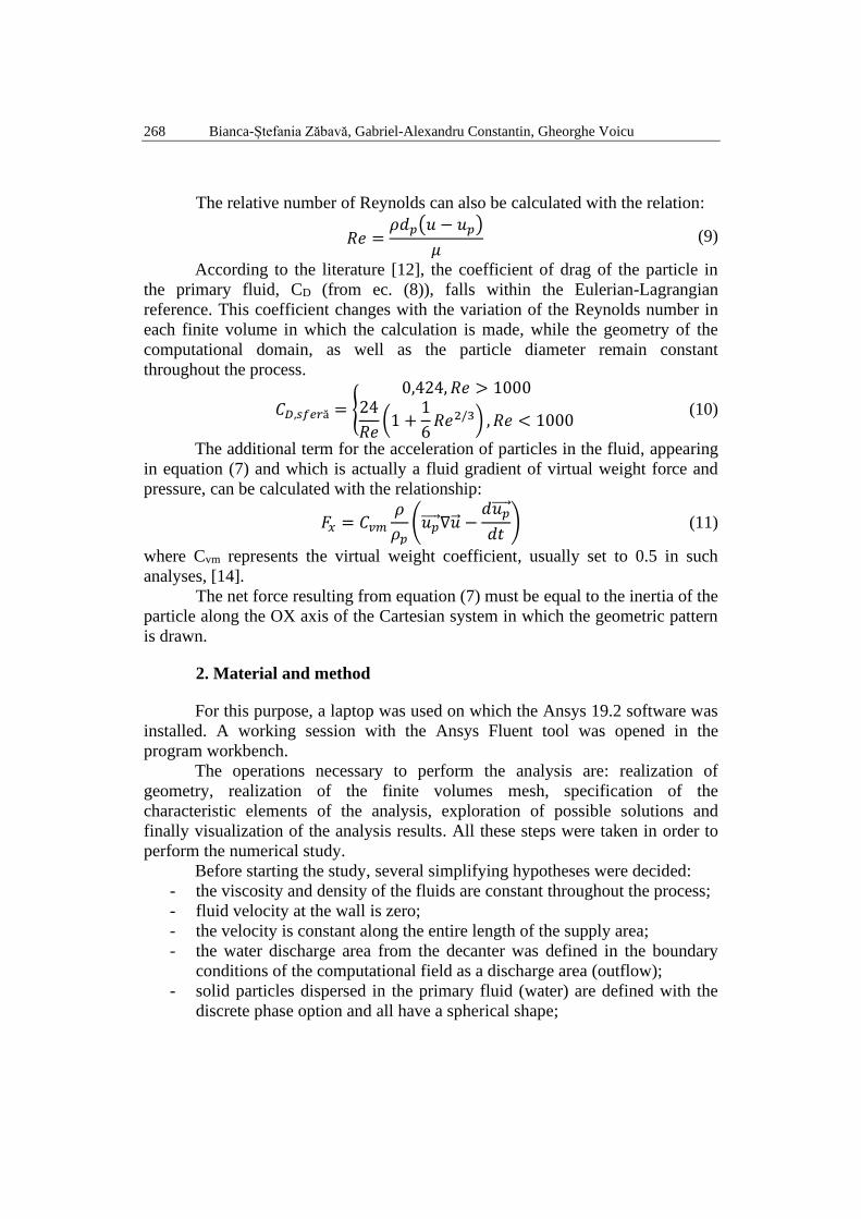
The relative number of Reynolds can also be calculated with the relation:

𝑅𝑒 =𝜌𝑑𝑝(𝑢 − 𝑢𝑝)

𝜇 (9)

According to the literature [12], the coefficient of drag of the particle in

the primary fluid, CD (from ec. (8)), falls within the Eulerian-Lagrangian

reference. This coefficient changes with the variation of the Reynolds number in

each finite volume in which the calculation is made, while the geometry of the

computational domain, as well as the particle diameter remain constant

throughout the process.

𝐶𝐷,𝑠𝑓𝑒𝑟ă = {0,424, 𝑅𝑒 > 1000

24

𝑅𝑒(1 +

1

6𝑅𝑒2/3) , 𝑅𝑒 < 1000

(10)

The additional term for the acceleration of particles in the fluid, appearing

in equation (7) and which is actually a fluid gradient of virtual weight force and

pressure, can be calculated with the relationship:

𝐹𝑥 = 𝐶𝑣𝑚

𝜌

𝜌𝑝(𝑢𝑝⃗⃗ ⃗⃗ ∇�⃗� −

𝑑𝑢𝑝⃗⃗ ⃗⃗

𝑑𝑡) (11)

where Cvm represents the virtual weight coefficient, usually set to 0.5 in such

analyses, [14].

The net force resulting from equation (7) must be equal to the inertia of the

particle along the OX axis of the Cartesian system in which the geometric pattern

is drawn.

2. Material and method

For this purpose, a laptop was used on which the Ansys 19.2 software was

installed. A working session with the Ansys Fluent tool was opened in the

program workbench.

The operations necessary to perform the analysis are: realization of

geometry, realization of the finite volumes mesh, specification of the

characteristic elements of the analysis, exploration of possible solutions and

finally visualization of the analysis results. All these steps were taken in order to

perform the numerical study.

Before starting the study, several simplifying hypotheses were decided:

- the viscosity and density of the fluids are constant throughout the process;

- fluid velocity at the wall is zero;

- the velocity is constant along the entire length of the supply area;

- the water discharge area from the decanter was defined in the boundary

conditions of the computational field as a discharge area (outflow);

- solid particles dispersed in the primary fluid (water) are defined with the

discrete phase option and all have a spherical shape;


- the analysis will be done 2D in the middle area of the radial decanter.

After establishing the steps to be followed, the geometric modelling of the

2D view of the decanter was started.

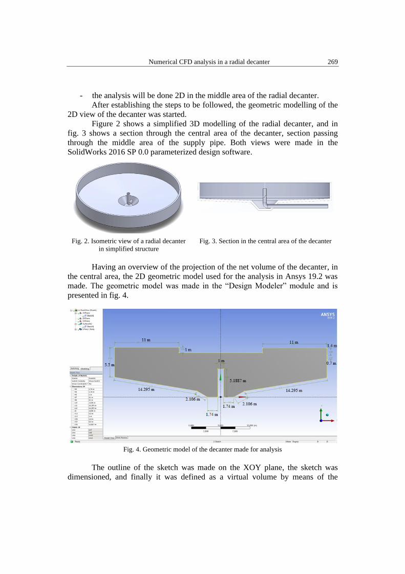
Figure 2 shows a simplified 3D modelling of the radial decanter, and in

fig. 3 shows a section through the central area of the decanter, section passing

through the middle area of the supply pipe. Both views were made in the

SolidWorks 2016 SP 0.0 parameterized design software.

Fig. 2. Isometric view of a radial decanter

in simplified structure

Fig. 3. Section in the central area of the decanter

Having an overview of the projection of the net volume of the decanter, in

the central area, the 2D geometric model used for the analysis in Ansys 19.2 was

made. The geometric model was made in the “Design Modeler” module and is

presented in fig. 4.

Fig. 4. Geometric model of the decanter made for analysis

The outline of the sketch was made on the XOY plane, the sketch was

dimensioned, and finally it was defined as a virtual volume by means of the


surface tool in the sketch („surfaces from sketches”). It should be noted that the

sketch is in fact a 2D view of the projection of the net volume of the decanter in

the central area.

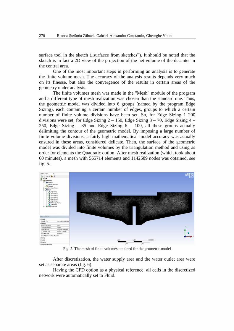
One of the most important steps in performing an analysis is to generate

the finite volume mesh. The accuracy of the analysis results depends very much

on its finesse, but also the convergence of the results in certain areas of the

geometry under analysis.

The finite volumes mesh was made in the "Mesh" module of the program

and a different type of mesh realization was chosen than the standard one. Thus,

the geometric model was divided into 6 groups (named by the program Edge

Sizing), each containing a certain number of edges, groups to which a certain

number of finite volume divisions have been set. So, for Edge Sizing 1 200

divisions were set, for Edge Sizing 2 – 150, Edge Sizing 3 – 70, Edge Sizing 4 –

250, Edge Sizing – 35 and Edge Sizing 6 – 100, all these groups actually

delimiting the contour of the geometric model. By imposing a large number of

finite volume divisions, a fairly high mathematical model accuracy was actually

ensured in these areas, considered delicate. Then, the surface of the geometric

model was divided into finite volumes by the triangulation method and using as

order for elements the Quadratic option. After mesh realization (which took about

60 minutes), a mesh with 565714 elements and 1142589 nodes was obtained, see

fig. 5.

Fig. 5. The mesh of finite volumes obtained for the geometric model

After discretization, the water supply area and the water outlet area were

set as separate areas (fig. 6).

Having the CFD option as a physical reference, all cells in the discretized

network were automatically set to Fluid.


Fig. 6. Water supply and water outlet area

Further, the discretized geometric model was loaded into the "Setup"

module to establish the analysis conditions. Time was first set as Transient to

allow particles to move through the fluid mass, and the gravitational acceleration

was set on the OY axis with value -9.81 m/s2 because the water supply is in the

opposite direction to the gravitational force.

Knowing the diameter of the supply pipe in the decanter (1 m), water

density (1000 kg/m3), water viscosity (8.9·10-4 m²/s) and the maximum water

speed in the velocity area (0.036 m/s according to [17]), it was possible to

calculate the Reynolds number in the supply area in the decanter. This is equal to

40449.44, which frames the flow regime as turbulent. As a result, the

mathematical model k-ε (2 equations) was chosen to substantiate the study. To

increase the accuracy of the study was selected as a model k-ε the option RNG

(Re-Normalisation Group). This is a method of renormalizing the Navier-Stokes

equations to explain the effects of smaller scales of motion and was first proposed

in the paper [18]. In the standard model k-ε, the eddy viscosity is determined from

a single turbulence length scale, so that the calculated turbulent diffusion is that

which occurs only at the specified scale, while in reality all scales of motion will

contribute to turbulent diffusion. RNG approach, which is a mathematical

technique that can be used to obtain a turbulence model similar to k-ε, results in a

modified form of the epsilon equation that tries to explain the different scales of

motion by changes in the production term, [19].

The behavior of the fluid near the walls was set as standard, and the

constants in the equations k-ε have been set as shown above.

With the choice of the mathematical model, particle injection was also

required. As a result, the discrete phase has been activated (Discrete Phase – On),

the material to be injected into the water supply area has been chosen (calcium


carbonate), the injection position has been set, particle diameter (max. 0.001 m),

flow rate (0.1 kg/s), the time interval for the injection (from 0 to 10 s simulation

time) and collision behaviour. The primary fluid was then set by choosing the

water-liquid option from the Ansys software library.

Next, was proceeded to establish the boundary conditions of the

simulation. Thus, the water supply area has been set as the supply region with the

velocity-inlet option and it has established a primary fluid supply velocity of

0.036 m/s, and the water outlet area has been set as the outlet area with the

outflow option. The operating conditions (pressure and gravitational acceleration)

were also set here.

Subsequently, the method of analysis was chosen. Thus, for the pressure,

momentum, turbulent kinetic energy and dissipation rate, the second order

equations were selected in order to obtain the highest possible calculation

accuracy.

After initializing the calculus, the calculation parameters were set and the

calculation was run. The step size of the calculation has been set to 0.005 s, the

number of steps to 2000 and the number of iterations per time step at 20. By

multiplying the size of the calculation step (0.005 s) with the number of steps

(2000) the total simulation time is obtained (10 s). The calculation was started by

pressing the Calculate button.

During the calculation, the software draws in real time the curves of

variation of the residual values. It should be noted that the total calculation time

was 26.5 hours.

A residual value is defined as the difference between the actual value and

the forecasted value, [20]. The closer the residual values are to zero, the more

convergent the results. In this analysis it can be seen that the residual values have

reached a value of 10-5 which is quite satisfying.

3. Results and discussions

After completing the calculation, the simulation results were visualized.

Ansys 19.2 software also presents the results in the form of coloured contours, the

value of each coloured region being given in a chromatic legend, but also in the

form of charts or histograms. The results obtained are presented below. It should

be noted that the maximum values appear in the water supply area, as well as in

the outlet area.

In figure 7 the distribution of the dynamic pressure in the liquid mass is

presented. It can be easily seen that the maximum values are reached in the

feeding area inside the decanter, absolutely logical thing anyway, because in this

area the highest deformation rate is also reached (fig. 8).


Fig. 7. Dynamic pressure

The pressure distribution is oriented towards the outlet area of the

decanter, the liquid moving more in this direction.

Fig. 8. Fluid strain rate at 10 seconds of simulation

Maximum fluid velocity values are obtained in the same areas (water

supply area and outlet area), generally due to deformation of the liquid. Fig. 9

shows the velocity magnitude distribution in the supply area

Fig. 9. Velocity magnitude


Figure 10 shows the mean velocity magnitude along the length of the

radial decanter.

Fig. 10. Mean velocity magnitude

The distribution of turbulent kinetic energy is shown in fig. 11. With its

help, the areas with the highest potential for hydrodynamic losses can be

observed, losses that favour the sedimentation process. In order to produce as few

vortices as possible it is desirable that the sedimentation process be carried out in

the presence of a turbulent kinetic energy, of the lowest possible value.

Fig. 11. Turbulent kinetic energy

The distribution of turbulence intensity is shown in fig. 12. The maximum

percentage values (9.6%) are also obtained in the supply area.


Fig. 12. Turbulence intensity

4. Conclusions

In the paper, the numerical CFD analysis in a radial decanter was

performed.

This type of study should be performed for any constructive variant of

decanters. It is quite important to identify areas of turbulence. In these areas the

velocity of the fluid, dynamic pressure in fluid, but also its strain rate increases,

which leads to a propagation of turbulence throughout the mass of liquid. As the

rate of occurrence of vortices in the mass of liquid is greater, thus decreasing the

probability of settling those heavy particles that should settle as quickly as

possible at the bottom of the decanter.

For the decanter analysed in this paper, which has values of turbulence

intensity of up to 9.6%, especially in the water supply area, it is recommended to

increase the diameter of the supply pipe in the supply area, but keeping the flow

rate. By increasing the diameter only in the supply area, lower liquid flow velocity

will be obtained, which will reduce the likelihood of vortices occurrence.

R E F E R E N C E S

[1].***ANSYS, Computational Fluid Dynamics (CFD) Simulation

https://www.ansys.com/products/fluids.

[2]. *** ANALYSIS TOOLS, ANSYS Advantage - Volume II, Issue 4, 2008.

[3]. A. H. Ghawi and J. Kriš, “A Computational Fluid Dynamics Model of Flow and Settling in

Sedimentation Tanks”, Applied Computational Fluid Dynamics, Prof. Hyoung Woo Oh

(Ed.) , InTech, March 2012, pp. 19-34, ISBN: 978-953-51- 0271-7.


[4]. H. Gao and M. K. Stenstrom, “Evaluating the Effects of Inlet Geometry on the Limiting Flux

of Secondary Settling Tanks with CFD Model and 1D Flux Theory Model”, in J. Environ.

Eng., vol. 145, nr. 10, 2019.

[5]. P. Larsen, “On the hydraulics of rectangular settling basins, experimental and theoretical

studies”. Report no. 1001, in Dept of Water Resour Engrg, Lund Inst of Tech, Lund Univ,

Lund, Sweden, 1977.

[6]. S. Das, H. Bai, C. Wu, et al., “Improving the performance of industrial clarifiers using three

dimensional computational fluid dynamics”,in Eng. Appl. Comput. Fluid Mech., vol. 10,

nr. 1, 2016, pp. 130-144, DOI: 10.1080/19942060.2015.1121518.

[7]. M.E. Valle Medina, “Secondary settling tanks modeling : study of the dynamics of activated

sludge sedimentation by computational fluids dynamics”, Chemical and Process

Engineering. Université de Strasbourg, 2019.

[8]. A.A. Al-Jeebory, J. Kris and J.H. Ghawi, “Performance improvement of water treatment plants

in Iraq by CFD model”, in Al-Qadisiya Journal For Engineering Sciences, vol. 3, nr. 1,

2010, pp. 1–13.

[9].A.G. Ghawi and J. Kriš, “Improvement performance of secondary clarifiers by a computational

fluid dynamics model”, in SJCE, vol. 19, nr. 4, , 2011, pp. 1–11.

[10]. K. Ramalingam, S. Xanthos, M. Gong, et al., “Critical modeling parameters identified for

3D CFD modeling of rectangular final settling tanks for New York city wastewater

treatment plants”, in Water Sci. Technol., vol. 65, nr. 6, 2012, pp. 1087–1094.

[11]. D. Lo, New flocculation centre well design for circular final clarifiers at the Tai Po Sewage

Treatment Works”, in HKIE Transactions, vol. 20, nr. 4, 2013, pp. 221–229.

[12]. Kh. Sharifi, T. Jafari Behbahani, S. Ebrahimi, et al., “A new computational fluid dynamics

study of a liquid-liquid hydrocyclone in the two phase case for separation of oil droplets and

water”, in Braz. J. Chem. Eng., vol. 36, nr. 4, Oct./Dec. 2019, pp. 1601-1612,

https://doi.org/10.1590/0104-6632.20190364s20170619.

[13]. Andrew Parry , “Numerical Simulations and Optimisation of Gas-Solid-Liquid Separator”,

MSc Thesys in Petroleum Engineering, , Imperial College London, 2014.

[14]. Peter Kohnke, “ANSYS Theory Reference”, Eleventh Edition, SAS IP, Inc, 1999.

http://research.me.udel.edu/~lwang/teaching/MEx81/ansys56manual.pdf.

[15]. Daniel Brennan, “The numerical simulation of two-phase flows in settling tanks”, PhD

Thesys, University of London, 2001.

[16]. *** American Meteorological Society (AMS) - Glossary of Meteorology, 2012.

[17]. H.A.M. Heikal, A.A. El-Hafiz, A.R. El Baz, et al., “Study the performance of circular clarifier

in existing potable water treatment plant by using computational fluid dynamics”, ,in

IWRA, XVI World Water Congress Cancun, Quintana Roo. Mexico, 29 May – 3 June,

2017.

[18]. V. Yakhot, S.A. Orszag, S. Thangam, et al., "Development of turbulence models for shear

flows by a double expansion technique", in Phys. Fluids., vol. 4, no. 7, 1992, pp. 1510-

1520.

[19]. *** https://www.cfd-online.com/Wiki/RNG_k-epsilon_model

[20]. *** https://stattrek.com/regression/residual-analysis.aspx

http://research.me.udel.edu/~lwang/teaching/MEx81/ansys56manual.pdf

NUMERICAL CFD ANALYSIS IN A RADIAL DECANTER

Documents

Transcript of NUMERICAL CFD ANALYSIS IN A RADIAL DECANTER