Nuclear Structure Erich Ormand N-Division, Physics and Adv. Technologies Directorate Lawrence...

Nuclear StructureErich Ormand

N-Division, Physics and Adv. Technologies DirectorateLawrence Livermore National Laboratory

This work was carried out under the auspices of the U.S. Department of Energy by the University of California, Lawrence Livermore National Laboratory under contract No. W-7405-Eng-48.

This document was prepared as an account of work sponsored by an agency of the United States Government. Neither the United States Government nor the University of California nor any of their employees, makes any warranty, express or implied, or assumes any legal liability or responsibility for the accuracy, completeness, or usefulness of any information, apparatus, product, or process disclosed, or represents that its use would not infringe privately owned rights. Reference herein to any specific commercial product, process, or service by trade name, trademark, manufacturer, or otherwise, does not necessarily constitute or imply its endorsement, recommendation, or favoring by the United States Government or the University of California. The views and opinions of authors expressed herein do not necessarily state or reflect those of the United States Government or the University of California, and shall not be used for advertising or product endorsement purposes.

15thNational Nuclear Physics15thNational Nuclear PhysicsSummer SchoolSummer School

June 15-27, 2003June 15-27, 2003

Lecture #2

22

Low-lying structure – The interacting Shell Model

• The interacting shell model is one of the most powerful tools available too us to describe the low-lying structure of light nuclei

• We start at the usual place:

• Construct many-body states |i so that

• Calculate Hamiltonian matrix Hij=j|H|i— Diagonalize to obtain eigenvalues

€

H =r p i

2

2m+ U ri( )

⎛

⎝ ⎜

⎞

⎠ ⎟

i

∑ + VNN

r r i −

r r j( )

i< j

∑ − U ri( )i

∑

0s N=0

0d1s N=2

0f1p N=4

1p N=1

€

Ψi = Cinφn

n

∑

⎟⎟⎟⎟⎟

⎠

⎞

⎜⎜⎜⎜⎜

⎝

⎛

NNN

N

HH

HH

HHH

K

OM

L

1

2221

11211

We want an accurate description of low-lying states

€

φ= 1

A!

φi r1( ) φi r2( ) K φi rA( )

φ j r1( ) φ j r2( ) φ j rA( )

M O M

φl r1( ) φl r2( ) K φl rA( )

= al+K a j

+ai+ 0

33

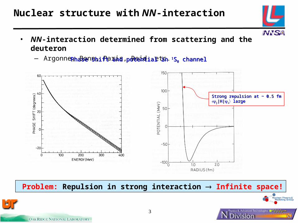
Nuclear structure with NN-interaction

• NN-interaction determined from scattering and the deuteron— Argonne, Bonn, Paris, Reid, etc.

Problem: Repulsion in strong interaction Infinite space!

Phase shift and potential in Phase shift and potential in 11SS00 channel channel

Strong repulsion at ~ 0.5 fmStrong repulsion at ~ 0.5 fmjj|H||H|ii large large

44

Can we get around this problem?Effective interactions

• Choose subspace of for a calculation (P-space)— Include most of the relevant physics — Q -space (excluded - infinite)

• Effective interaction:

— Two approaches:– Bloch-Horowitz

– Lee-Suzuki:

nφ

iiieff EH Ψ=Ψ P̂P̂

PHHE

HHHi

effˆQ̂

Q̂

1P̂P̂

−+=

QP

HHeffeff==PPXXHHXX-1-1PP

⇒klGij ++ ++ +…+…

QQXXHHXX-1-1PP=0=0

55

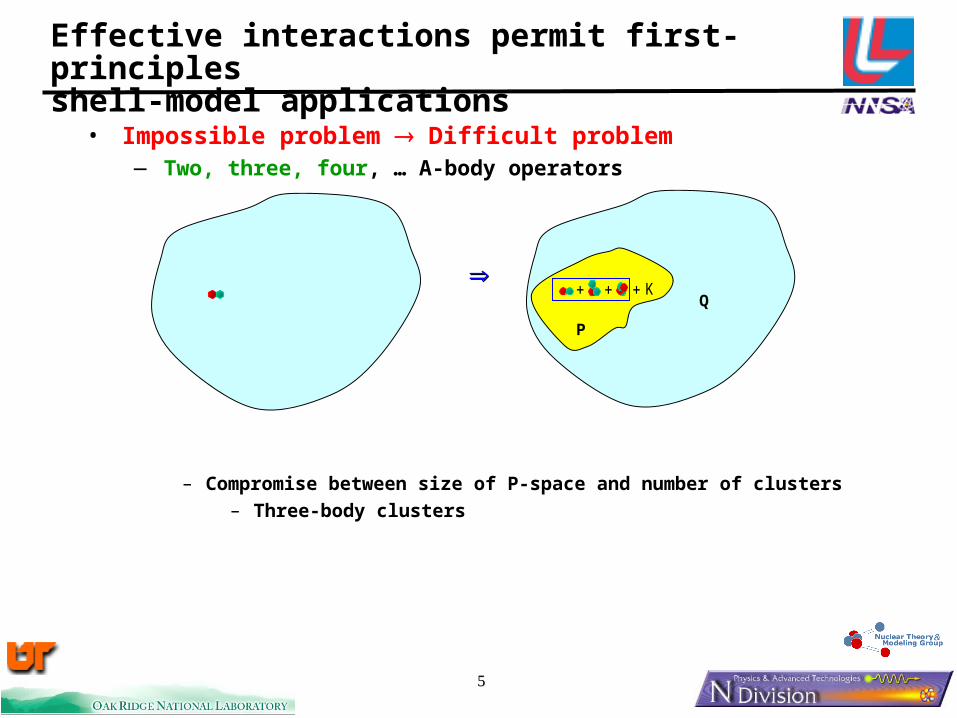
Effective interactions permit first-principles shell-model applications

• Impossible problem Difficult problem— Two, three, four, … A-body operators

– Compromise between size of P-space and number of clusters

– Three-body clusters

Q

P

K+++

66

23

2

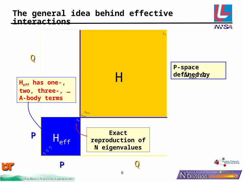
The general idea behind effective interactions

HeffQXHX-1P=0

H

QQ

PP

QQPP

P-space defined by ΩhmaxN

23

Exact reproduction of N eigenvalues

Heff has one-, two, three-, … A-body terms

77

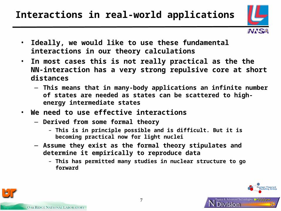
Interactions in real-world applications

• Ideally, we would like to use these fundamental interactions in our theory calculations

• In most cases this is not really practical as the the NN-interaction has a very strong repulsive core at short distances

— This means that in many-body applications an infinite number of states are needed as states can be scattered to high-energy intermediate states

• We need to use effective interactions— Derived from some formal theory

– This is in principle possible and is difficult. But it is becoming practical now for light nuclei

— Assume they exist as the formal theory stipulates and determine it empirically to reproduce data

– This has permitted many studies in nuclear structure to go forward

88

Shell model applications

• The practical Shell Model1. Choose a model space to be used for a range of nuclei

– E.g., the 0d and 1s orbits (sd-shell) for 16O to 40Ca or the 0f and 1p orbits for 40Ca to 120Nd

2. We start from the premise that the effective interaction exists

3. We use effective interaction theory to make a first approximation (G-matrix)

4. Then tune specific matrix elements to reproduce known experimental levels

5. With this empirical interaction, then extrapolate to all nuclei within the chosen model space

6. Note that radial wave functions are explicitly not included, so we add them in later

The empirical shell model works well!But be careful to know the limitations!More on exact treatments later.

99

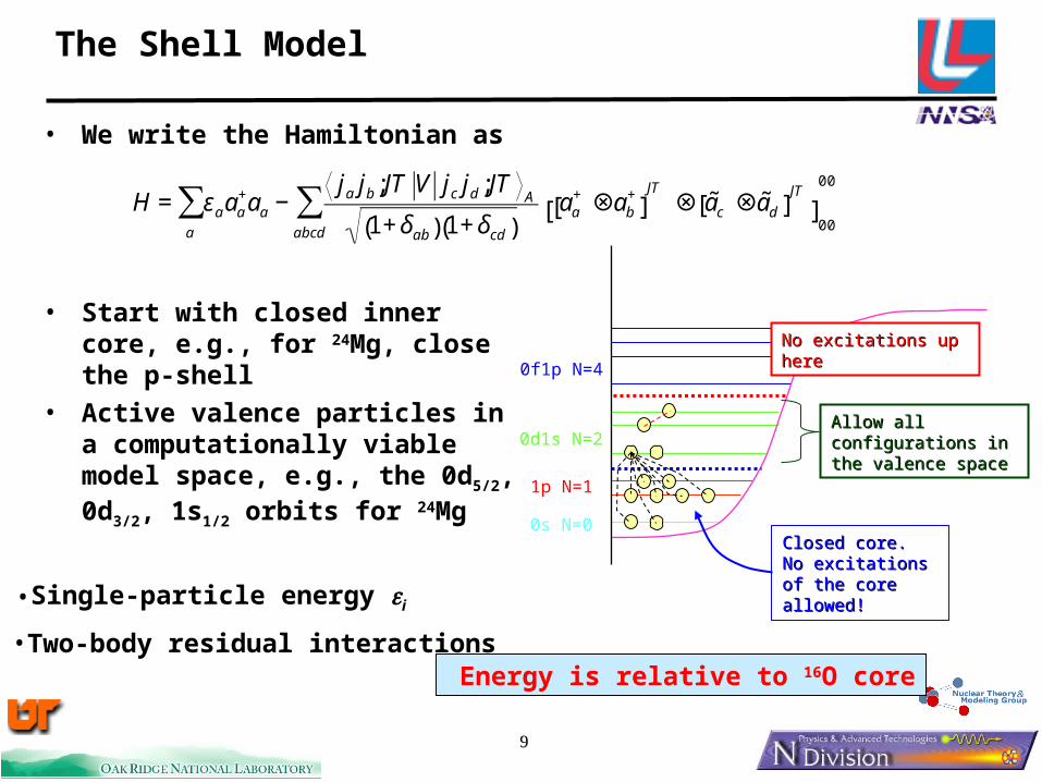
The Shell Model

• We write the Hamiltonian as

• Start with closed inner core, e.g., for 24Mg, close the p-shell

• Active valence particles in a computationally viable model space, e.g., the 0d5/2, 0d3/2, 1s1/2 orbits for 24Mg

€

H = εaaa+aa

a

∑ −ja jb ;JT V jc jd ;JT

A

1+ δab( ) 1+ δcd( )aa

+ ⊗ ab+

[ ]JT⊗ ˜ a c ⊗ ˜ a d[ ]

JT

[ ]00

00

abcd

∑

0s N=0

0d1s N=2

0f1p N=4

1p N=1

Closed core.Closed core.No excitations of the No excitations of the core allowed!core allowed!

Allow all configurations Allow all configurations in the valence spacein the valence space

No excitations up hereNo excitations up here

•Single-particle energy i

•Two-body residual interactionsEnergy is relative to 16O core

00

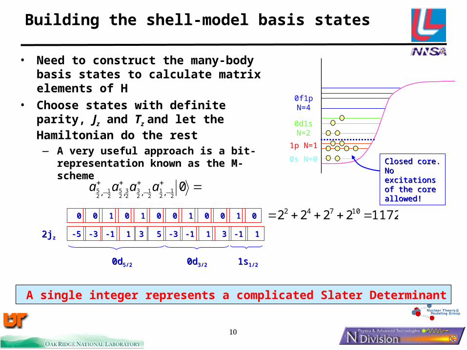
Building the shell-model basis states

• Need to construct the many-body basis states to calculate matrix elements of H

• Choose states with definite parity, Jz and Tz and let the Hamiltonian do the rest

— A very useful approach is a bit-representation known as the M-scheme

0s N=0

0d1s N=2

0f1p N=4

1p N=1

11722222 10742 =+++=2j2jzz

0d0d5/25/2 1s1s1/21/20d0d3/23/2

-5-5 -1-1-3-3 11 33 55 -1-1-3-3 11 33 -1-1 11

11 00 00 11 00 11 00 00 11 00 00 00

=+−

+−

++− 0

21

21

21

23

23

25

21

25 ,,,, aaaa

Closed core.Closed core.No excitations of No excitations of the core allowed!the core allowed!

A single integer represents a complicated Slater Determinant

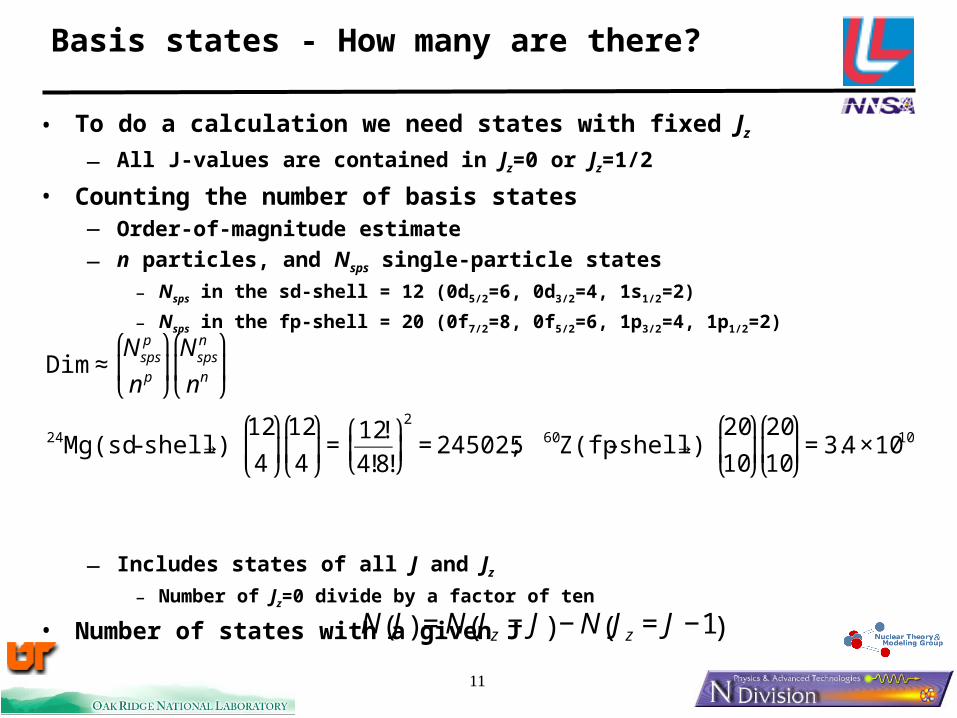
Basis states - How many are there?

• To do a calculation we need states with fixed Jz

— All J-values are contained in Jz=0 or Jz=1/2

• Counting the number of basis states— Order-of-magnitude estimate

— n particles, and Nsps single-particle states

– Nsps in the sd-shell = 12 (0d5/2=6, 0d3/2=4, 1s1/2=2)

– Nsps in the fp-shell = 20 (0f7/2=8, 0f5/2=6, 1p3/2=4, 1p1/2=2)

— Includes states of all J and Jz

– Number of Jz=0 divide by a factor of ten

• Number of states with a given J

€

Dim ≈Nsps

p

n p

⎛

⎝ ⎜

⎞

⎠ ⎟Nsps

n

nn

⎛

⎝ ⎜

⎞

⎠ ⎟

24 Mg(sd - shell) → 12

4

⎛

⎝ ⎜

⎞

⎠ ⎟12

4

⎛

⎝ ⎜

⎞

⎠ ⎟=

12!

4!8!

⎛

⎝ ⎜

⎞

⎠ ⎟2

= 245025; 60Z(fp - shell) → 20

10

⎛

⎝ ⎜

⎞

⎠ ⎟20

10

⎛

⎝ ⎜

⎞

⎠ ⎟= 3.4 ×1010

€

N J( ) = N Jz = J( ) − N Jz = J −1( )

22

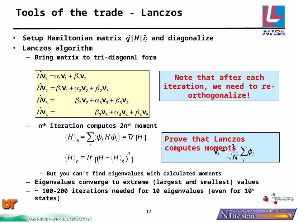
Tools of the trade - Lanczos

• Setup Hamiltonian matrix j|H|i and diagonalize

• Lanczos algorithm— Bring matrix to tri-diagonal form

— nth iteration computes 2nth moment

– But you can’t find eigenvalues with calculated moments

— Eigenvalues converge to extreme (largest and smallest) values— ~ 100-200 iterations needed for 10 eigenvalues (even for 108 states)

5444334

4333223

3222112

21111

ˆ

ˆ

ˆ

ˆ

vvvv

vvvv

vvvv

vvv

βαβ

βαβ

βαβ

βα

++=

++=

++=

+=

H

H

H

HNote that after each iteration, we need to re-orthogonalize!

€

H0

= ψ i Hψ i

i

∑ = Tr H[ ]

Hn

= Tr H − H0( )

n

[ ]

Prove that Lanczos computes moments -

€

vi =1

Nϕ i

i

∑

33

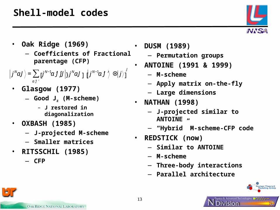
Shell-model codes

• Oak Ridge (1969)— Coefficients of Fractional

parentage (CFP)

• Glasgow (1977)— Good Jz (M-scheme)

– J restored in diagonalization

• OXBASH (1985)— J-projected M-scheme— Smaller matrices

• RITSSCHIL (1985)— CFP

• DUSM (1989)— Permutation groups

• ANTOINE (1991 & 1999)— M-scheme— Apply matrix on-the-fly— Large dimensions

• NATHAN (1998)— J-projected similar to ANTOINE— “Hybrid” M-scheme-CFP code

• REDSTICK (now)— Similar to ANTOINE— M-scheme— Three-body interactions— Parallel architecture

€

jNαJ = jN−1 ′ α ′ J jJ } jNαJ[ ] jN−1 ′ α ′ J ⊗ j[ ]J

′ α ′ J

∑

44

REDSTICK – basis state ordering

• Ordering of basis states speeds up the calculation

• Need a FAST lookup scheme

• Construct proton and neutron many-body Slater determinants

— Order by Parity, Jz and Ωh

For each proton SD store start in For each proton SD store start in Lanczos vector: pos(Lanczos vector: pos(ii))For each neutron SD store relative For each neutron SD store relative position in Jz, parity list: pos(position in Jz, parity list: pos( jj))Position in Lanczos vector Position in Lanczos vector determined by summing two determined by summing two integers integers k= k= pos(pos(ii)+ )+ pos(pos(jj))Same algorithm can be used to Same algorithm can be used to sort and find two-body matrix sort and find two-body matrix elementselements

• Limits truncations— Partition truncations not

possible

• Much faster!

• Lanczos vector points to p & n SD’s (less memory)

ProtonsProtons NeutronsNeutrons

11

22

33

44

55

66

JJzz=1=1

JJzz=-1=-1

JJzz=0=0

JJzz=1=1

JJzz=-1=-1

JJzz=0=0

11

22

33

44

55

66

77

55

66

55

66

66

66

77

77

11

11

22

22

11

22

11

22

33

33

44

44

55

55

33

44

33

44

33

44

0+1=1

0+2=2

4+2=6

4+1=5

2+2=4

2+1=3

6+1=7

6+2=8

10+2=12

12+1=13

12+2=14

10+1=11

8+1=9

8+2=10

Lanczos vectorLanczos vector

55

• With large dimensions, it may be better not to pre-calculate and store the Hamiltonian matrix

• Find states connected by one-body proton or neutron operator

• pn-part is the hardest— Product of two one-body operators

– Pre-sort connections by one-body operators; store operator and phase

REDSTICK – Applying the Hamiltonian – pn partOn-the-fly

pnnl

nn

pk

pm vαβγδδγβα ννππ ΦΦΦΦ ++

Jump List #1 Jump List #2

Initial PN-SD

∑∑∑∑ Φ′=ΦΦΦ=Φ=j

jjj i

jiiii

ii cHccHH ˆˆv

∑ ++=ijkl

lkjipnijkl

pn vH ννππˆ

• Loop over all initial proton-neutron SD’s Φi=p

k nl

— For each pk loop over all p

m connected by one-body operator

– For each nl loop over all n

n connected by one-body operator but limited in Jz, parity, and by final proton state p

m

– Update Lanczos vector: Position=pos(pos(mm)+)+pos(pos(nn))

Ωh

66

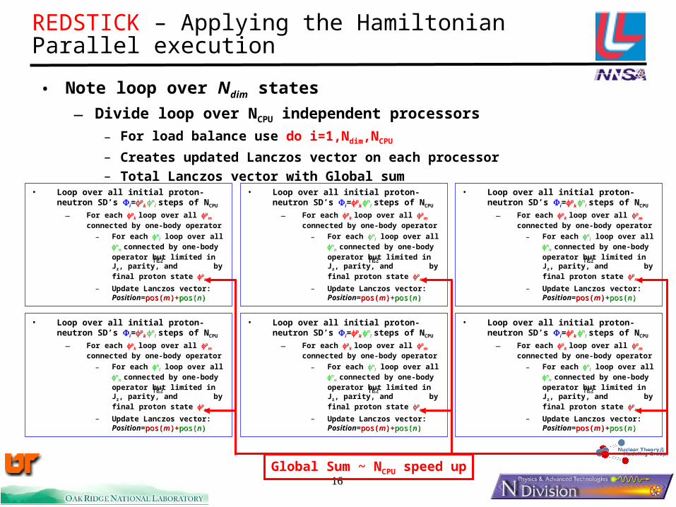
• Note loop over Ndim states

— Divide loop over NCPU independent processors

– For load balance use do i=1,Ndim,NCPU

– Creates updated Lanczos vector on each processor

– Total Lanczos vector with Global sum

REDSTICK – Applying the Hamiltonian Parallel execution


k nl steps of NCPU


m

connected by one-body operator


n

connected by one-body operator but limited in Jz, parity, and by final proton state p

m


Ωh


k nl steps of NCPU


m



n


m


Ωh


k nl steps of NCPU


m



n


m


Ωh


k nl steps of NCPU


m



n


m


Ωh


k nl steps of NCPU


m



n


m


Ωh


k nl steps of NCPU


m



n


m


Ωh

Global Sum ~ NCPU speed up

77

•

• Not that trivial (but also not the main bottleneck in the calculation)

• Let each processor be responsible for a sub set of Lanczos vectors written to disk

• Each processor has a copy of the current vector

• Accumulate sum overlaps on each node, n

• Global sum then and normalize

• Not quite the same as sequential reorthogonalization, but seems to work fine (also used in MFD).

REDSTICK – ReorthogonalizationParallel execution

∑<

⋅−=ji

jijj vvvv

∑<

⋅=ji

jin vva

∑=n

naa avv −= jj

88

Shell-model codes - Performance

REDSTICK or ANTOINE

99

Simple application of the shell model

• A=18, two-particle problem with 16O core— Two protons: 18Ne (T=1)— One Proton and one neutron: 18F (T=0 and T=1)— Two neutrons: 18O (T=1)

Example: 18O

• How many states for each Jz? How many states of each J?

— There are 14 states with Jz=0

– N(J=0)=3

– N(J=1)=2

– N(J=2)=5

– N(J=3)=2

– N(J=4)=2

Question # 1?

2020

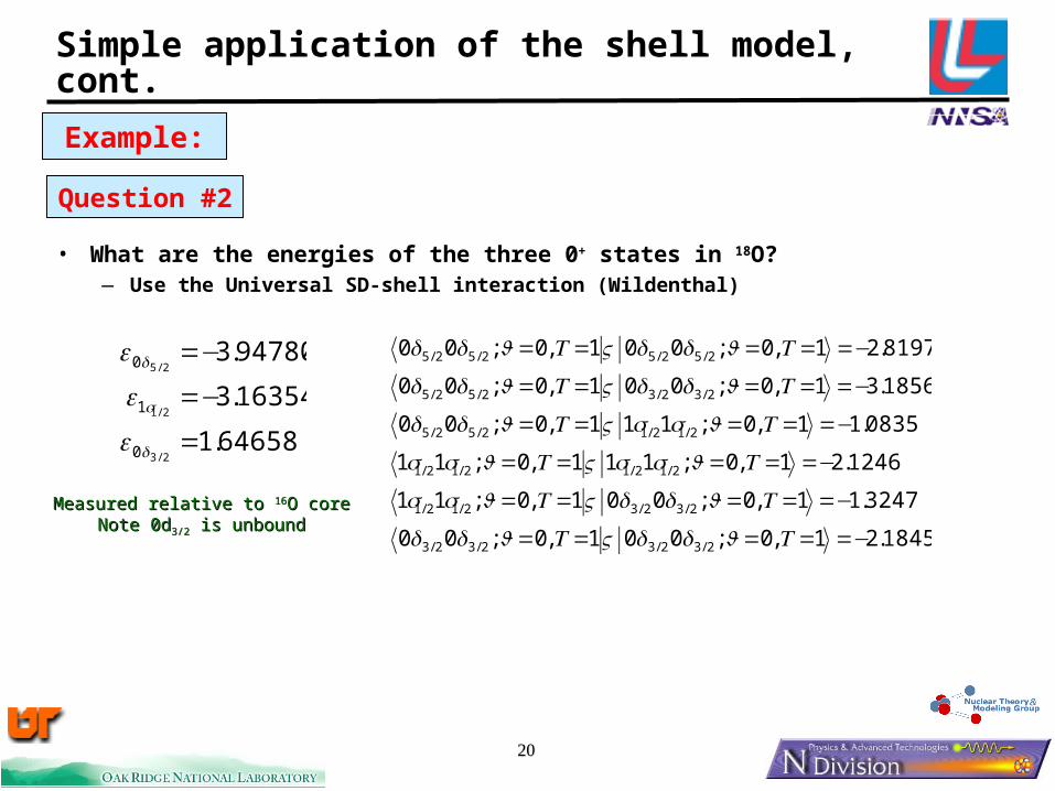
Simple application of the shell model, cont.

Example:

Question #2

• What are the energies of the three 0+ states in 18O?— Use the Universal SD-shell interaction (Wildenthal)

1845.21,0;001,0;00

3247.11,0;001,0;11

1246.21,0;111,0;11

0835.11,0;111,0;00

1856.31,0;001,0;00

8197.21,0;001,0;00

2/32/32/32/3

2/32/32/12/1

2/12/12/12/1

2/12/12/52/5

2/32/32/52/5

2/52/52/52/5

−=====

−=====

−=====

−=====

−=====

−=====

TJddVTJdd

TJddVTJss

TJssVTJss

TJssVTJdd

TJddVTJdd

TJddVTJdd

64658.1

16354.3

94780.3

2/3

2/1

2/5

0

1

0

=

−=

−=

d

s

d

Measured relative to Measured relative to 1616O coreO coreNote 0dNote 0d3/23/2 is unbound is unbound

22

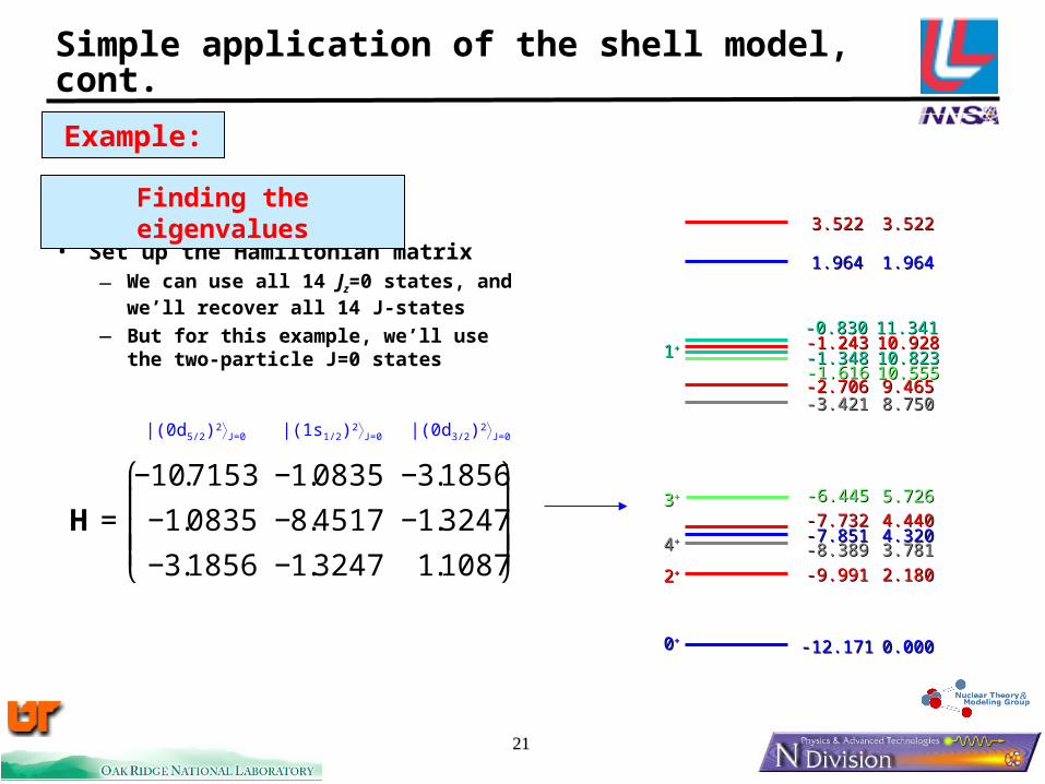
Simple application of the shell model, cont.

Example:

• Set up the Hamiltonian matrix— We can use all 14 Jz=0 states, and

we’ll recover all 14 J-states— But for this example, we’ll use

the two-particle J=0 states

Finding the eigenvalues

€

H =

−10.7153 −1.0835 −3.1856

−1.0835 −8.4517 −1.3247

−3.1856 −1.3247 1.1087

⎛

⎝

⎜ ⎜ ⎜

⎞

⎠

⎟ ⎟ ⎟

00++ -12.171-12.171 0.0000.000

-7.851-7.851 4.3204.320

1.9641.964 1.9641.964

-1.616-1.616 10.55510.555

-6.445-6.445 5.7265.72633++

-8.389-8.389 3.7813.781

-3.421-3.421 8.7508.750

44++

-9.991-9.991 2.1802.180

-7.732-7.732 4.4404.440

-1.243-1.243 10.92810.928

3.5223.522 3.5223.522

-2.706-2.706 9.4659.465

22++

-1.348-1.348 10.82310.823

-0.830-0.830 11.34111.341

11++

|(0d5/2)2J=0 |(1s1/2)2J=0 |(0d3/2)2J=0

2222

€

Qe−ωHeωP = 0; ω = QωP

α Q ω α P = α Q k ˜ k α P

k

d P

∑ ; ˜ k α P α P ′ k α P

∑ = δk ′ k

β P Heff α P = β P 1+ ω+ω( )−1 2

′ α P ′ α P ˜ k E k˜ k ′ ′ α P ′ ′ α P 1+ ω+ω( )

−1 2α P

′ ′ α P

∑′ α P

∑k

dP

∑

β P 1+ ω+ω( ) α P = β P˜ k ˜ k α P

k

d P

∑Hermitian effective interactionHermitian effective interaction

The matrix βP|Heff|αP exactly reproduces dp solutions of the full problem

• Choose P-space for A-body calculation, with dimension dp

— P-space basis states: and Q-space basis states:

— Need dP solutions, |k, in the “infinite” space, i.e.,

— Write X=e-

€

H k = Ek k

€

αP

€

αQ

Effective interactions with the Lee-Suzuki method

2323

For an n-body cluster in Heff, we must first solve the n-body problem!

• Find Hn-eff iteratively

— n-particles bound in oscillator potential

• Steps:

— A=2 H2-eff

— Use H2-eff for A=3

H3-eff

— Use H3-eff for A=4

H4-eff

2424

Effective interactions really work

• 4He with the effective-field theory Idaho-A potential

•Effective interactions improve convergence!•Are EFT potentials useful for nuclear-structure studies?

2525

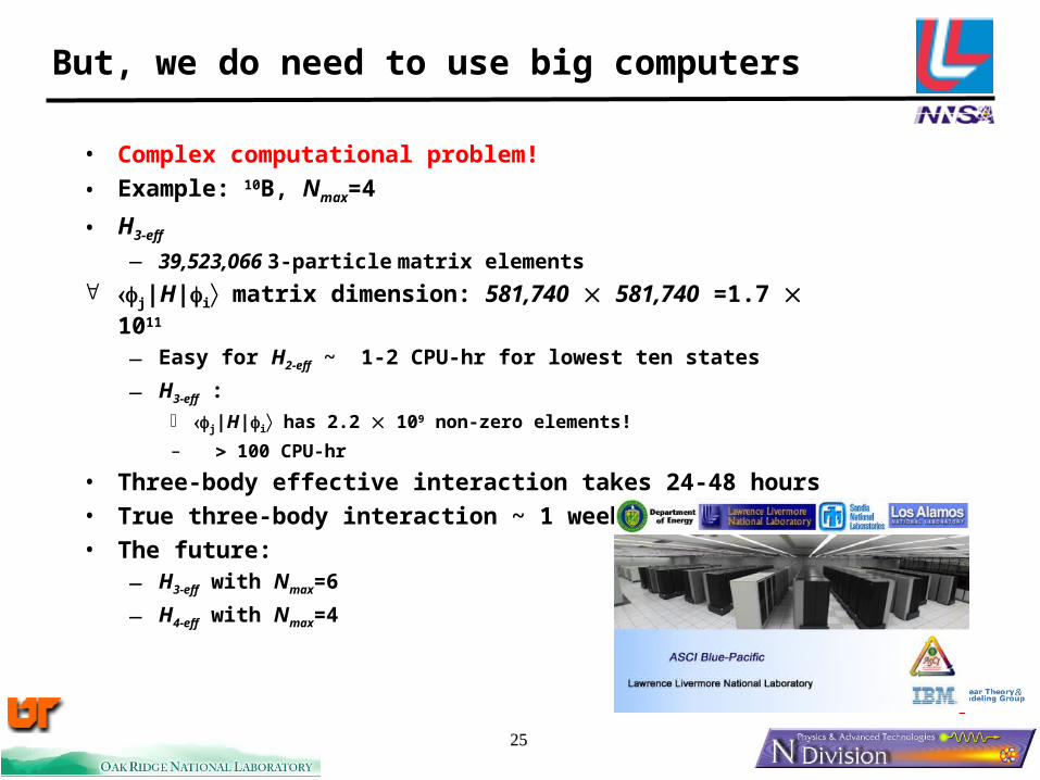
But, we do need to use big computers

• Complex computational problem!

• Example: 10B, Nmax=4

• H3-eff

— 39,523,066 3-particle matrix elements

j|H|i matrix dimension: 581,740 581,740 =1.7 1011

— Easy for H2-eff ~ 1-2 CPU-hr for lowest ten states

— H3-eff : j|H|i has 2.2 109 non-zero elements!

– 100 CPU-hr

• Three-body effective interaction takes 24-48 hours• True three-body interaction ~ 1 week• The future:

— H3-eff with Nmax=6

— H4-eff with Nmax=4

2626

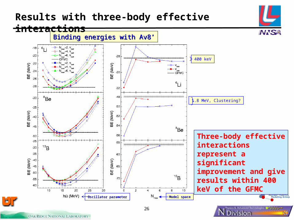
Binding energies with Av8’Binding energies with Av8’

Results with three-body effective interactions

400 keV

1.8 MeV, Clustering?

Oscillator parameterOscillator parameter Model spaceModel space

Three-body effective interactions represent a significant improvement and give results within 400 keV of the GFMC

2727

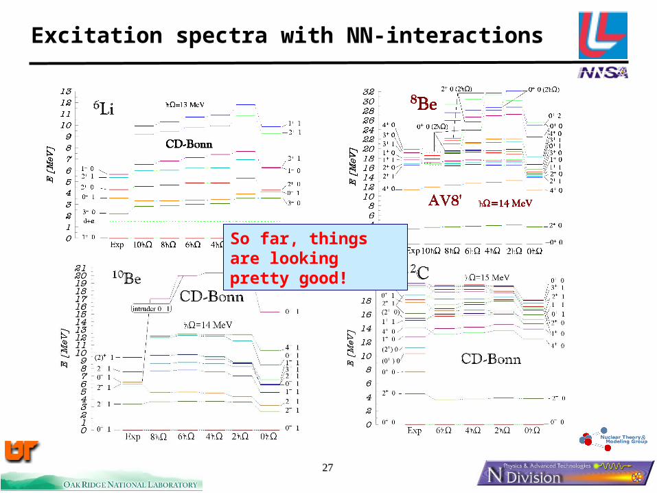
Excitation spectra with NN-interactions

So far, things are looking pretty good!

2828

Excitation spectrum of 8Be

• Experiments hint at a new excited state in 8Be

— Excitation energy ~10-30 MeV

• Previous theory studies were unable to predict the existence of such a state

• In large model spaces we find an intruder band

— model space and 2108 basis states!

— No-core ANTIONE

Ωh10

2929

Excitation spectrum of 8Be

I

JJE

2

)1( +=

dd00++

44++

22++

Rotational Band

oror

9-10 MeV9-10 MeV

0 2 4 6 8 10 12 14 160

5

10

15

20

25

30

Ex0+

(MeV)

Nmax

Shell-Model Exponential 1/N

max

Gaussian

• What is the nature of this state?

— Is it real?– Stable 0+, 2+, 4+ rotational

band

–

– Ex appears to be stabilizing

– ~10-15 MeV

— Beta-vibration of the ground-state αα cluster?

– Excitation energy seems too high

— Super-deformed prolate shape?

-1 MeV 1.11~ h−I

3030

The NN-interaction clearly has problems

Note inversion of spins!

•The NN-interaction by itself does not describe nuclear structure•Also true for A=11

33

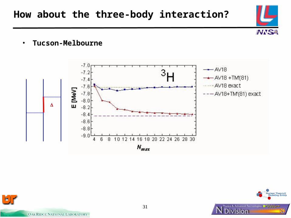
How about the three-body interaction?

• Tucson-Melbourne

3232

Three-body interaction in a nucleus

The three-nucleon interaction plays a critical role in determining the structure of nuclei

3333

More on three-body interactions in a nucleus

• Gamow-Teller and M1 transitions

— Sensitive to spin-orbit force— Because is a generator of

SU(4) and transitions in different representations are forbidden, i.e., B(GT)=0!!

— NN-interaction tends to preserve SU(4)

— Spin-orbit breaks SU(4)

The three-nucleon interaction has a strong spin-orbit component

3434

Summary of ab initio studies

• Extensions and improvements:— Determine the form of the NNN-interaction— Implementation of effective operators for transitions— Four-body effective interactions— Effective field-theory potentials; are they any good for structure?— Integrate the structure into some reaction models (R-matrix)

• Questions and open problems to be addressed:— Is it possible to improve the mean field?— Can we improve the convergence of the higher states?— Unbound states. Can we use a continuum shell model?— How high in A can we go?— Can we use this method to derive effective interactions for

conventional nuclear structure studies?

Ωh

• Significant progress towards an exact understanding of nuclear structure is being made!

• These are exciting times!!

Nuclear Structure Erich Ormand N-Division, Physics and Adv. Technologies Directorate Lawrence...

Documents

Transcript of Nuclear Structure Erich Ormand N-Division, Physics and Adv. Technologies Directorate Lawrence...