NPS ARCHIVE1997. OC*BENNETT, R.

JNAVAL POSTGRADUATE SCHOOLMonterey, California

THESIS

CLASSIFICATION OF UNDERWATER SIGNALSUSING A BACK-PROPAGATIONNEURAL NETWORK

by

Richard Campbell Bennett Jr.

June, 1997

Thesis Advisor:

Co-Advisor:

Monique P. Fargues

Roberto Cristi

Approved for public release; distribution is unlimited.

ThesisB3767

*AVA' POSTGRADUATE >CH0O

lONTERENO #943-5101

DUDLEY KNOX LIBRARYNAVAL POSTGRADUATE SCHOOLMONTEREY, CA 93943-5101

REPORT DOCUMENTATION PAGE Form Approved OMB No. 0704-0188

Public reporting burden for this collection of information u estimated to average 1 hour per response, including the time for reviewing instruction, searching existing data

sources, gathering and maintaining the data needed, and completing and reviewing the collection of information. Send comments regarding this burden estimate or any

other aspect of this collection of information, including suggestions for reducing this burden, to Washington Headquarters Services, Directorate for Information

Operations and Reports. 1215 Jefferson Davis Highway. Suite 1204. Arlington. VA 22202-4302. and to the Office of Management and Budget, Paperwork Reduction

Project (0704-0188) Washington DC 20503.

1.

blank)

AGENCY USE ONLY (Leave REPORT DATEJune 1997

3. REPORT TYPE AND DATES COVEREDMaster's Thesis

4. TITLE AND SUBTITLE: CLASSIFICATION OF UNDERWATER SIGNALS USING

A BACK-PROPAGATION NEURAL NETWORK

6. AUTHOR(S) Bennett, Richard Campbell, Jr.

5. FUNDING NUMBERS

7. PERFORMING ORGANIZATION NAME(S) AND ADDRESS(ES)

Naval Postgraduate School

Monterey CA 93943-5000

8. PERFORMING ORGANIZATIONREPORT NUMBER

9. SPONSORING/MONITORING AGENCY NAME(S) AND ADDRESS(ES) 10. SPONSORING/MONITORING

AGENCY REPORT NUMBER

11. SUPPLEMENTARY NOTES The views expressed in this thesis are those of the author and do not reflect the

official policy or position of the Department of Defense or the U.S. Government.

12a. DISTRIBUTION/AVAILABILITY STATEMENTApproved for public release; distribution is unlimited.

12b. DISTRIBUTION CODE

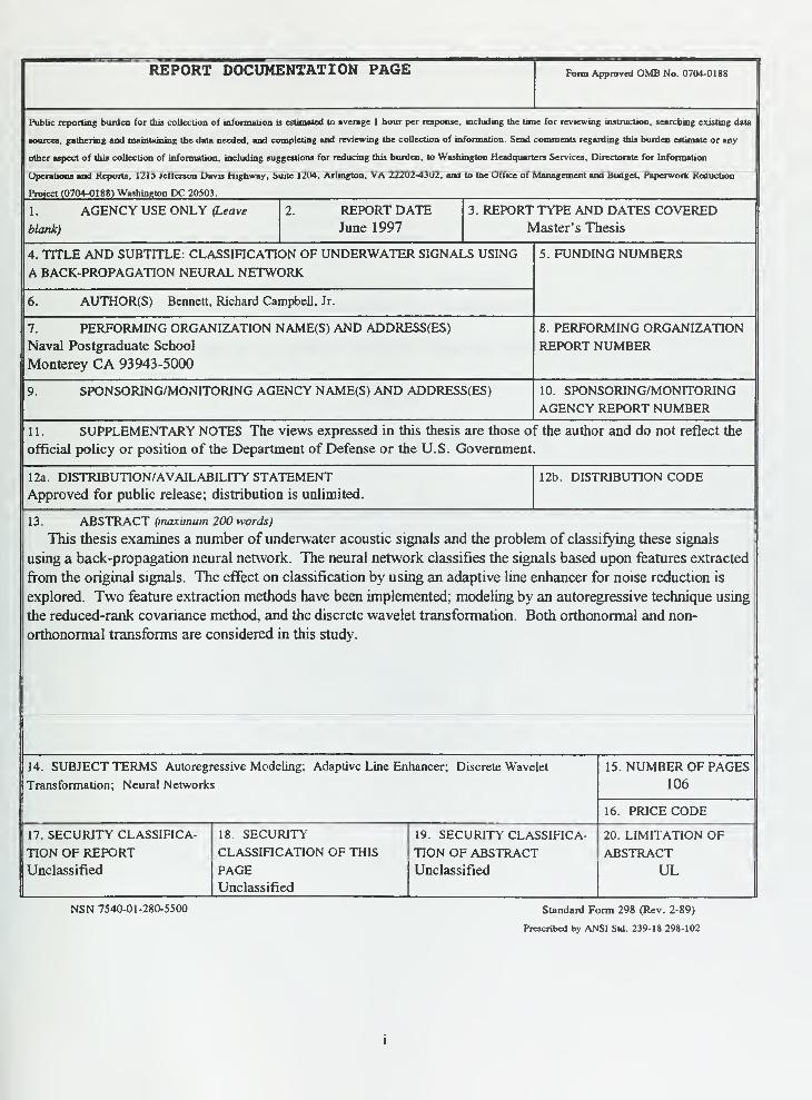
13. ABSTRACT (maximum 200 words)

This thesis examines a number of underwater acoustic signals and the problem of classifying these signals

using a back-propagation neural network. The neural network classifies the signals based upon features extracted

from the original signals. The effect on classification by using an adaptive line enhancer for noise reduction is

explored. Two feature extraction methods have been implemented; modeling by an autoregressive technique using

the reduced-rank covariance method, and the discrete wavelet transformation. Both orthonormal and non-

orthonormal transforms are considered in this study.

14. SUBJECT TERMS Autoregressive Modeling; Adaptive Line Enhancer; Discrete Wavelet

Transformation; Neural Networks

15. NUMBER OF PAGES106

16. PRICE CODE

17. SECURITY CLASSIFICA-

TION OF REPORTUnclassified

18. SECURITY

CLASSIFICATION OF THIS

PAGEUnclassified

19. SECURITY CLASSIFICA-

TION OF ABSTRACTUnclassified

20. LIMITATION OFABSTRACT

UL

NSN 7540-01-280-5500 Standard Form 298 (Rev. 2-89)

Prescribed by ANSI Std. 239-18 298-102

Approved for public release; distribution is unlimited.

CLASSIFICATION OF UNDERWATER SIGNALS USING A BACK-PROPAGATION NEURAL NETWORK

Richard Campbell Bennett, Jr.

Lieutenant, United States Navy

B.E., State University of New York Maritime College, 1987

Submitted in partial fulfillment

of the requirements for the degree of

MASTER OF SCIENCE IN ELECTRICAL ENGINEERING

from the

NAVAL POSTGRADUATE SCHOOLJune, 1997

DUDLEY KNOX LIBRARY '^SSB^S^naval postgraduate school $^9?tgrMMTESCHOOMONTEREY, CA 93943-5101 KJNfEREY CA 93943-5101

ABSTRACT

This thesis examines a number of underwater acoustic signals and the problem of classifying

these signals using a back-propagation neural network. The neural network classifies the signals

based upon features extracted from the original signals. The effect on classification by using an

adaptive line enhancer for noise reduction is explored. Two feature extraction methods have been

implemented; modeling by an autoregressive technique using the reduced-rank covariance method,

and the discrete wavelet transformation. Both orthonormal and non-orthonormal transforms are

considered in this study.

VI

TABLE OF CONTENTS

L INTRODUCTION 1

IL SIGNAL SELECTION 3

m. FEATURE EXTRACTION OF BIOLOGICAL AND SEISMIC SIGNALS 5

A. INTRODUCTION 5

B. NOISE REDUCTION USING ADAPTIVE LINE ENHANCEMENT 6

1. Introduction 6

2. LeastMean Square Algorithm 6

3. Adaptive Line Enhancement Using the LMSAlgorithm 8

C. REDUCED-RANK AUTOREGRESSIVE MODELING 16

1. Introduction 16

2. Autoregressive Modeling 16

3. The Covariance Method. 18

4. Model Order Selection 19

5. Reduced-Rank Covariance Method. 21

D. THE DISCRETE WAVELET TRANSFORMATION 26

1. Introduction 26

2. The Continuous Wavelet Transform And Series. 27

3. Discrete Wavelet Transform 29

4. Multiresolution Algorithm 30

5. The A-Trous Algorithm 33

IV. CLASSIFICATION VIA BACK-PROPAGATION NEURAL NETWORK. 37

A. INTRODUCTION 37

B. THE BACK-PROPAGATION NEURAL NETWORK 37

1. The Processing Element. 38

2. The Transfer Function 39

3. The Normalized-Cumulative Delta Learning Rule , 40

4. MinMax Tables. 41

5. Network Architecture 41

6. The Classification Rate 43

7. Training and Testing The Neural Network. 43

V. RESULTS 47

A. PERFORMANCE RESULTS OBTAINED USING REDUCED-RANK ARCOEFFICIENTS 49

1. No ALE Preprocessing 49

2. ALE Preprocessing Applied to Data 57

B. CLASSIFICATION RESULTS OBTAINED WITH WAVELET-TYPE PARAMETERS.. 5

3

7. Orthogonal Wavelet Decomposition 53

2. Non-Orthogonal A-Trous Wavelet Decomposition 61

C. CLASSIFICATION RESULTS OBTAINED BY COMBINING AR COEFFICIENTS ANDORTHONORMAL WAVELET-TYPE PARAMETERS 69

7. No ALE Pre-processing Applied to the Data 69

2. ALE Pre-processing Applied to the Data 71

VL CONCLUSION AND RECOMMENDATIONS 73

A. CONCLUSION 73

B. RECOMMENDATIONS 75

vn

APPENDIX 77

ORDER.M 77

BURG_A.M 78

ARWHALE.M 78

SVD_COV.M 79

LMSALE.M 81

ECOEFF2.M 83

INWVLET.M 84

SHENDWT2.M 85

LOADW3V7T.M 88

SPECT.M 90

CALLOUT.M 91

OUTNNR.M 94

REFERENCES 95

INITIAL DISTRIBUTION LIST 97

vui

I. INTRODUCTION

A. SCOPE OF STUDY

The United States Navy's undersea acoustic surveillance systems were used during the

Cold War to detect and track enemy submarine activities. These systems consist of both fixed and

mobile hydrophone arrays. Many aspects of these arrays are now declassified and are being used

by geophysicists to monitor undersea earthquakes and volcanoes. The undersea SOund

Surveillance System (SOSUS), array out of Whidbey Island Washington is of interest to this

thesis. It consists of fixed hydrophones mounted at the approximate depth of the deep sound

channel. These hydrophones are very sensitive and have the ability to pick up very low frequency

sounds.[13 p. 3]

Earthquakes have associated with them three phases, representing three separate types of

energy release. First is the primary phase, or p-phase. This phase consists of energy that is

transmitted as compressed shock waves within the earth's crust. The secondary, or s-phase,

consists of transverse shock waves also being transmitted through the earth's crust. The last

phase, the tertiary or t-phase, is only associated with underwater earthquakes. The t-phase consists

of acoustic energy that is transmitted into the water column from the shaking ocean floor. The

definition has been expanded recently to include any low-frequency seismic event that transmits

acoustic energy into the water column. [13 p. 4]

The National Oceanic and Atmospheric Administration (NOAA), Pacific Marine

Environmental Laboratory is conducting a study of underwater geological processes, such as

earthquakes and volcanic activities using the Whidbey Island SOSUS array. This undersea

surveillance system also has great potential for use in tracking and estimating populations of

marine mammals. The purpose of this thesis is to investigate classification procedures which

would allow for proper separation of geological processes and biological signals, and would

classify the various biological signals for further biological studies. A Neural Network (NN)

configuration is chosen in this study to automate the classification process. NN have great

potentials in automatic classification problems, as they can learn through examples and do not

require a precise mathematical model for the signal characteristics. However, NN implementations

require the set of training data to be representative of the various signals to be classified to have

good performance. Thus, the success of any classification scheme depends on a judicious choice of

unique features that allows the classifier to discriminate between each class of interest. This thesis

explores the use of autoregressive (AR) modeling and wavelet decomposition as feature extraction

techniques. In addition, we investigate the application of an adaptive line enhancer to de-noise the

underwater data. The AR coefficients used as NN inputs are computed using a reduced-rank

covariance method. This technique combines traditional covariance method and the singular value

decomposition to reduce the effect of noise in the signal model. Next, orthogonal and non-

orthogonal implementations of the discrete wavelet transform are chosen as feature extractors. The

orthogonal decomposition uses two different wavelet bases; Symmlet 8, and Coiflet 3 coefficients.

The A-Trous implementation of the non-orthogonal decomposition uses a modified Morlet wavelet.

This classification study uses 5 different species of whale (Sperm, Killer, Humpback, Gray, and

Pilot Whale) and underwater earthquake data.

Chapter II describes the methodology used in the signal selection. Chapter III presents the

analytical methods used to compute the input parameters to the Neural Network implementation.

In this chapter, we first describe the adaptive line enhancer procedure designed to reduce the effects

to wideband noise contained in the recordings. Next, we present the reduced-rank covariance AR

modeling technique. Finally, we briefly review multiresolution algorithms and present their

application to our classification problem. Chapter IV describes the back-propagation neural

network implementation used during our study. Results are presented in Chapter V. Last, Chapter

VI presents conclusions and recommendations for further study.

II. SIGNAL SELECTION

The operating environment of the undersea sonar array is in the Pacific Northwest, off the

coast of Whidbey Island Washington. Researchers familiar with the array data have indicated the

presence of marine mammal sounds in the recordings, as this array is located in a whale migration

route. Thus, this system has a high potential for use in marine mammal studies. In order to separate

underwater seismic data from marine mammal sounds, we selected recordings from a cross section of

whale species that represent the population in the array system area during the yearly migration

periods. The frequency characteristics of the various whale species cover the entire frequency

spectrum. The biological signals range from very short pulses to long melodic songs. In addition to

the underwater earthquake used, the types of biological signals chosen for the study are: Sperm

Whale, Killer Whale, Humpback Whale, Gray Whale, and Pilot Whale.

Note that even though the array data indicates the presence of some species of whale

sounds, the biological and earthquake signals used were obtained from a different source [12]. The

decision not to use biological cuts obtained from the system array data was motivated by the fact

that we were unable to obtain proper identification of the various species of whales by a specialist.

Thus, in order to minimize any problems due to incorrect training we used cuts from a commercial

audio cassette in which the whale species have been properly identified. Each recording varied in

length from fifteen to thirty seconds. The recordings were of real, open ocean encounters from

various signal collection platforms. The signals, as an artifact of how they were collected, were all

corrupted with background noises. The corruption of the signals includes sounds from ships, small

boats, and other disturbances occurring in the natural environment, plus artificial noise from the

means of collection.

Each signal was digitized on a 486 PC using a Media Vision Pro Audio Spectrum sound card

at 8 kHz, using a single channel and 8 bits per sample. This ensured audio compatibility with the Sun

workstation's audio playback which is limited to single channel and 8 bit, 8 kHz data. The digitized

recordings were then processed to extract, as close as possible, the whale signals from the recordings,

using audio, and visualizations of the time and frequency domains. The whale 'songs' were then

selected and separated from the various other auditory manifestations of whale sounds. Next, these

sample songs were pasted together to make a nearly continuous song for each species. The sperm

whale signal was of a different nature. The recording is of the animals' echo ranging sonar. The very

short, rapid pulses were all kept intact. The earthquake recording was also kept intact. The pilot

whale sound produced a challenge as it was very short in duration, has high pitch, and was buried in

noise. It was especially difficult to separate the background noise from the pilot whale signal. Figure

2-1 presents typical time domain-plots from each class of signal studied.

Time Domain Signals

100

-1000.5 1 1.5 2 2.5

Samples Sperm Whale3 3.5 A

1001 i, ji i ,i i i i

100 L i i i t '

0.5 1 1.5 2 2.5Samples Killer Whale

3 3.5 A

100

1

1

|i i i '

i

O

100i

0.5 1 1.5 2 2.5 3 3.5 ASamples Humpback Whale v m4

1001

O -

1001 1 i i i ' I

-

0.5 1.5 2 2.5Samples Gray Whale

3.5

y 1Q100

-100

,, nU , .iumftMM ii I

o 0.5

mwh i i mmi Miii^U 'l

1.5 2 2.5Samples Pilot Whale

3.5

1.5 2 2.5Samples Earthquake x 10

Figure 2-1 Time domain signals of: a) sperm whale, b) killer whale, c) humpback whale, d) gray

whale, e) pilot whale, and f) earthquake.

In this chapter we have identified the signals that we are to classify. Next in Chapter HI,

we introduce the methods of feature extraction used in this study. Specifically we present the

reduced rank AR modeling technique, the discrete wavelet transform producing wavelet based

parameters, and the adaptive line enhancer to reduce the effects of wide-band noise contained in the

signals.

III. FEATURE EXTRACTION OF BIOLOGICAL AND SEISMICSIGNALS

A. INTRODUCTION

The biological and seismic signals used in this study consist of data records that typically

exceed 40,000 data points, which precludes any realistic method for classification based on the

data directly. Therefore signal characteristics need to be expressed in ways that retain the signals'

unique features, yet drastically reduce the amount of data needed as inputs to the classifier.

Feature extraction methods are a means of modeling a signal based on some specific property of

the signal. These features are then used to classify the signal.

One of the most distinguishing features of an acoustic signal is its spectral content. The

signals investigated in this study are generated by resonating cavities, vibrating vocal cords, and in

the case of seismic signals, the vibration of rock formations rubbing against each other. As a

result, most of the energy contained in the signals under study is concentrated in a few frequency

components. Note that an exception to this is the sperm whale data, which contains a very wide

spectral content. As a result, spectral information can be used to distinguish between the different

classes of signals. Two different procedures are considered in the study to extract frequency based

information. First we apply a reduced-rank AR modeling technique to compute AR coefficients

which are used as inputs to the neural network classifier. Next, we use the discrete wavelet

transform to compute wavelet-based parameters which are used as inputs to the NN. In addition,

we investigate the application of an adaptive line enhancer (ALE) algorithm as a pre-processing

step to reduce the effects due to wide-band noise contained in the data. This chapter presents the

feature extraction methods used in this study. The first part of this chapter presents the ALE noise

reduction procedure. Next, we present the reduced-rank autoregressive modeling. The discrete

wavelet transformation and its application to our study is presented last.

B. NOISE REDUCTION USING ADAPTIVE LINE ENHANCEMENT

1. Introduction

This study investigates the application of an Adaptive Line Enhancement (ALE) algorithm

to decrease the effect due to wideband noise present in the signals under study. The ALE algorithm

is a gradient descent, adaptive filter based on the least mean square (LMS) algorithm. The

algorithm tracks narrowband frequencies contained in the input signal, and removes wideband

components that are uncorrected to the frequencies present. First, we briefly review the concept of

the LMS algorithm, and next we present its application in the ALE algorithm.

2. Least Mean Square Algorithm

The motivation for the least mean square algorithm is to design a filter that learns from its

environment and converges to the optimum weight values given by the Wiener-Hopf equations in a

stationary environment. The LMS algorithm is a stochastic gradient-based algorithm which is

simple to implement and is effective in its ability to adapt to the external environment.

a. Overview Of The Structure And Operation of the LMS Algorithm

The system building blocks for the LMS algorithm are depicted in Figure 3-1

below. A similar block diagram will be shown later for the ALE implementation. The input signal

is fed into an adaptive FIR filter, and the output of the filter, y(n), is compared to the desired

signal, d(n), forming the error e(n). The second important feature of this scheme is the adaptive

control process where the filter weights are updated based on the direction needed to minimize the

mean square error. The filter weights are updated in accordance with:

w(n + \) = w(n) + -H[-VJ(n)], (3.1)

where vv(n) is the filter weight vector, |i is the step size parameter, and VJ(n) is the gradient of the

mean square error function. The negative gradient of the mean square error function ,

-VJ(n), is approximated by the instantaneous gradient expression:

-VJ{n)~2u{n)-e\n), (3.2)

where u(n)=[u(n), u(n-\), ... ,u(n-P+\)]T

, and P is the length of the filter.

Input u[n]

d[n]

Figure 3-1 The LMS Algorithm.

Thus the LMS estimated weight vector is obtained using the instantaneous gradient and is given

by:

w(« + 1) = w(n) + /je* (n)u(n) . (3.3)

The LMS weight coefficients are given by:

wk(n + \) = wk

(ri) + fju{n-k)e*{n). k = 0,l,...,P-l (3.4)

The step size parameter, u., is defined as a positive real constant which controls the size of

the incremental weight correction, and is bound by:

0<H<1

PRu (0)

(3.5)

to insure that the algorithm converges. Note that the LMS weights exhibit a random motion

around the optimal solution due to of the instantaneous approximation of the gradient, also known

as gradient noise. [3, p. 300]

The LMS algorithm is implemented as follows [3, p. 332]:

1) At time n=0, initialize the weight vector to an estimate of w(0)

2) y(n)= w H(n)u(n)

3) e(n) = d(n)-y(n)

4) w(n+l) = vv (n) +|iu(n)e*(n)

where the parameters of the algorithm to be chosen by the user are the length of the filter, P, and

the step size parameter, \i.

3. Adaptive Line Enhancement Using the LMS Algorithm

The adaptive line enhancer using the LMS algorithm is a logical choice to reduce the

wideband noise inherent in the sampled recordings. The motivation behind using the LMS

algorithm is that it is simple to implement, and has been historically proven to achieve satisfactory

performance. When used in the right conditions, the results can be of high quality.

The signals under investigation vary widely in nature from very localized in time (broad

frequency range), in the case of the sperm whale, to very localized in frequency (slowly changing in

time), in case of the humpback whale. Thus the step size was chosen to be 0.05 percent of the total

signal power as a result of a trial and error process.

The number of filter weights was chosen to decrease the total number of frequency related

components contained in the signals, and yet preserve enough to be able to discriminate between

each class of signal. This study uses a filter length of 10 to extract the five most dominant

sinusoids in each signal class. The figure below represents the implementation of the ALE

algorithm to estimate the signals present in the biologic and seismic data.

Input Signal u[n] Delay A u[n-A] Filter y[n]

Adaptive

Control Alg

Figure 3-2 The Adaptive Line Enhancer.

The delay A, shifts the signal in time causing the broadband noise contained in u(n-A) to

become uncorrelated with the broadband noise contained in the reference signal d(n) = u(n). By

experimentation we found that a delay of one sample was sufficient to decrease the contribution of

broadband noise without distorting the sperm whale data.

The output of the filter reflects only the signal that is correlated to the desired signal,

provided the filter is operating optimally. The MATLAB® program used in this study

LMSALE.M was written by LT D. Brown, USN [14] and is included in the appendix. The

following spectrograms represent the signals before and after applying the ALE algorithm. Note

that the results reflect the trade off in step size, filter length, and delay for all classes. This process

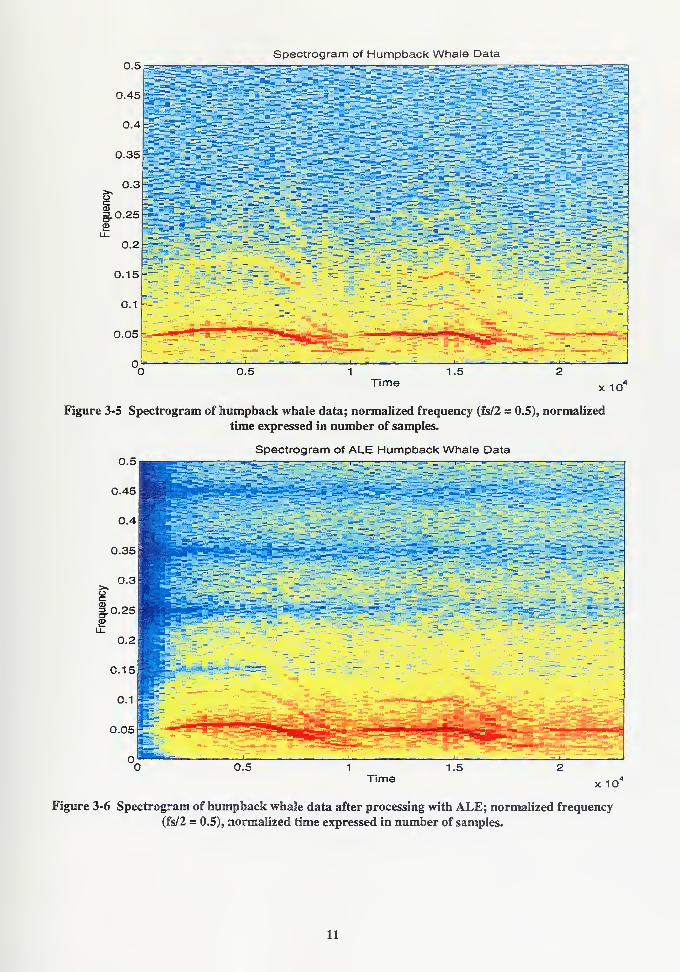
as implemented greatly improved the gray whale data, and had varying degrees of success for the

other classes.

Each of the following spectrograms was obtained using the MathWorks function

SPECGRAM.M. A Hanning window of size 512 with 50 % overlap is used and the FFT length

chosen is 5 1 2. Note that the spectrograms are given in terms of normalized frequency, where half

sampling frequency is represented by 0.5 and the time axis is expressed in terms of number of

samples. The spectral information is mapped to color values. The range of color values is red,

orange, yellow, green and blue. High intensity spectra appear as red. Low intensity spectra appear

as blue.

Spectrogram of Gray Whale Data

Time x 10

Figure 3-3 Spectrogram of gray whale data; frequency (fs/2 = 0.5), normalized time expressed in

number of samples.

Spectrogram of ALE Gray Whale Data

Time x 10

Figure 3-4 Spectrogram of gray whale data after processing with ALE; normalized frequency

(fs/2 = 0.5), normalized timeexpressed in normalized number of samples.

10

0.5

0.45

0.4

0.35

0.3

Spectrogram of Humpback Whale Data

mg.0.25CD

0.2

0.15

0.1

0.05 b-

0>

SSw5-^-

~ -

Time x 10

Figure 3-5 Spectrogram of humpback whale data; normalized frequency (fs/2 = 0.5), normalized

time expressed in number of samples.

Spectrogram of ALE Humpback Whale Data

1.5Time

x 10

Figure 3-6 Spectrogram of humpback whale data after processing with ALE; normalized frequency

(fs/2 = 0.5), normalized time expressed in number of samples.

11

0.5

0.45

0.4

0.35

0.3

Spectrogram of Pilot Whale Data

i—-r^p-

-^"-~ ~-~i -" - _ _ -

-r—_-__

"= -

r~~ -- - -

~»._R

-^ " -~==ss

Time x 10

Figure 3-7 Spectrogram of pilot whale data; normalized frequency (fs/2 = 05), normalized time

expressed in number of samples.

0.5Spectrogram of ALE Pilot Whale Data

Time x 10

Figure 3. -8 Spectrogram of pilot whale data after processing with ALE; normalized frequency

(fs/2 = 0.5), normalized time expressed in number of samples.

12

Spectrogram of Earthquake Data

Figure 3-9 Spectrogram of earthquake data; normalized frequency (fs/2 = 0.5), normalized time

expressed in number of samples.

Spectrogram of ALE Earthquake Data

Time x 10

Figure 3-10 Spectrogram of earthquake data after processing with ALE; normalized frequency

(fs/2 = 0.5), normalized time expressed in number of samples.

13

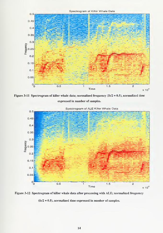
Spectrogram of Killer Whale Data

Time x 10

Figure 3-11 Spectrogram of killer whale data; normalized frequency (fs/2 = 0.5), normalized time

expressed in number of samples.

Spectrogram of ALE Killer Whale Data

Time x 10

Figure 3-12 Spectrogram of killer whale data after processing with ALE; normalized frequency

(fs/2 = 0.5), normalized time expressed in number of samples.

14

Spectrogram of Sperm Whale Data

Time x 10 in

Figure 3-13 Spectrogram of sperm whale data; frequency (fs/2 =0.5), normalized time expressed

number of samples.

Spectrogram of ALE Sperm Whale Data

Timex 10

Figure 3-14 Spectrogram of sperm 13 whale data after processing with ALE; normalized frequency

(fs/2 = 0.5), normalized time expressed in number of samples.

15

C. REDUCED-RANK AUTOREGRESSIVE MODELING

1

.

Introduction

The various classes of signals under investigation in this study exhibit differences in their

spectra, therefore spectral information is used for classification purposes. The autoregressive (AR)

coefficients of the filter used to model the original signal are the characterizing parameters chosen

as input parameters because they represent the spectra of the signals. They are used to classify the

various classes of signals under study.

In this section, we first introduce the concept of autoregressive modeling and the

covariance method used in this study. Next, we consider the problem of selecting the model order.

Finally, we present the application of reduced-rank modeling to the covariance method used to

decrease the effect of noise in the data.

2. Autoregressive Modeling

Autoregressive (AR) modeling is based on the idea that an original signal x(n) can be

expressed as the output of an all-pole linear shift invariant predictive filter driven by white noise.

In the time domain, this means that the signal x(n) may be expressed as a linear combination of

previous values x(n-i), i = 1,2, ... P, and some input noise sequence w(n).

p

x(n) = -1

£a(k)x(n-k) + b w(n), (3.6)

*=i

where P is the order of the predictor, b is the gain, and (a(l), ... , a(P)) are the coefficients of the

linear predictor to be determined. Taking the Z-transform of (3.6), the resulting transfer function

of the system used to generate x(n) from w(n) is given by:

X(z)=

b=

b

W(z) l + a1z~

i

+...+ap z'p

A{z)H(z)=-^- = - -H 7F = ^h- (3-7)

The AR coefficients can be obtained by solving a set of linear equations obtained from Equation

(3.6). Using the properties of the AR model, the correlation function Rx(/) obtained from x(n) is

given by:

Rx (l) = -alRx (l-l)—-aPRx (l-P) + b Rwx (l),

which leads to:

Rx (I) + a

xR

x (/ - 1)+- • +a PRx (/ - P) = b Rwx (I) . (3.8)

16

The cross correlation term Rwx(0 can be expressed as the convolution of the impulse response h(n)

of the AR system with the autocorrelation of the noise sequence Rw(n) as:

Rxw (l) = h(l)*Rw (l),

where Rw (l) = o 2J{l),

which leads to R^il) = h(l) cl8(l) = c 2Ji(l)

.

Thus,

Kx il) = olh\-l). (3.9)

By substituting (3.9) into (3.8), the correlation difference equation becomes:

Rx (l)+ a1Rx(l-l)+-+aPRx(l-P) = b a2

wh\-l). (3.10)

Note that h(n) is the impulse response of a causal filter, therefore h(n) is equal to for n < 0.

Next, using the Initial Value Theorem we have:

Kfc(0) = lim H(z)= lim

\ + alz~

l

+---+apzP (3.11)

Therefore,

Rwx (l) = for/>0.

Thus, Equation (3.10) becomes:

Rx (l) + a

}Rx (l -\)+—+a PRx (l - P) = b <j

2

w 8(l), for / > 0. (3.12)

Expressing Equations (3.12) for 1 = 0,..., P, leads to the extended set of Yule-Walker equations

[l.p.414]

Rx (0) *,(-l)

RX (V RAO)

RX (P) Rx(P-l)

RA-P)

Rx(-P + l)

RAO)

[1 'ol\bf'

ax =

ap

(3.13)

The set of AR coefficients of the filter a = [1, ai...,aP ] can be obtained by solving the set

of linear equations derived from Equation (3.13):

17

RAO) *,(-D

RAD Rx (0)

RAP-V RAP -2)

RA-p+iy <h 'RA+iy

RA-P + 2) a2 — — RA+2)

RAO) a P _RA+P).

(3.14)

Rx a = d

Note that in practical situations the true correlation matrix is usually not known and has to be

estimated from the observed data. Various estimation procedures have been considered in [1 ]. In

this study the covariance method is used to estimate the correlation matrix because no assumptions

are made about the data beyond the length of the prediction filter. Note that this is different from

the autocorrelation method where the data is zero padded.

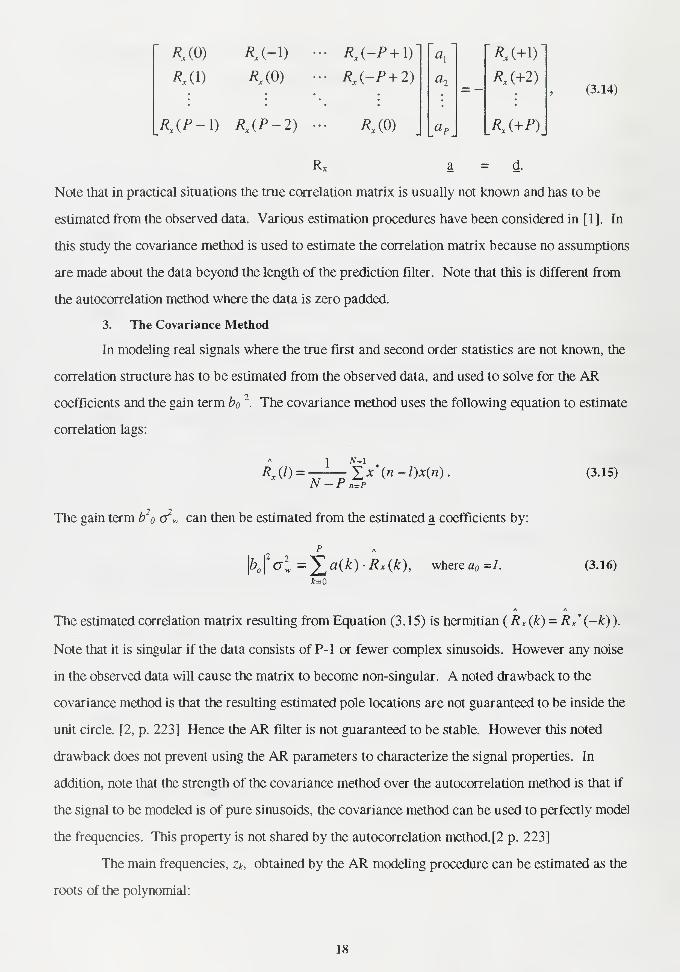
3. The Covariance Method

In modeling real signals where the true first and second order statistics are not known, the

correlation structure has to be estimated from the observed data, and used to solve for the AR

coefficients and the gain term bo2

. The covariance method uses the following equation to estimate

correlation lags:

RxQ) =TT-^N£x*(n-l)x(n).

N - P n=P

The gain term b' o*w can then be estimated from the estimated a coefficients by:

p|2 i

(3.15)

N °l> =^a(k) Rx(k), wherea =7. (3.16)

*=o

The estimated correlation matrix resulting from Equation (3. 15) is hermitian (R x (k) = R x* (-k) ).

Note that it is singular if the data consists of P-l or fewer complex sinusoids. However any noise

in the observed data will cause the matrix to become non-singular. A noted drawback to the

covariance method is that the resulting estimated pole locations are not guaranteed to be inside the

unit circle. [2, p. 223] Hence the AR filter is not guaranteed to be stable. However this noted

drawback does not prevent using the AR parameters to characterize the signal properties. In

addition, note that the strength of the covariance method over the autocorrelation method is that if

the signal to be modeled is of pure sinusoids, the covariance method can be used to perfectly model

the frequencies. This property is not shared by the autocorrelation method. [2 p. 223]

The main frequencies, Zk, obtained by the AR modeling procedure can be estimated as the

roots of the polynomial:

18

A(z) = l + a1z~

l

+---+aPz'P

. (3.17)

An estimate of the spectrum can be obtained from the recursive AR model:

x(n) + axx{n - 1)+- • +aPx{n -P) = e(n) (3.18)

where e(«) is the modeling error. Ideally z{n) is a Gaussian white noise sequence with a gain equal

to \b \

2oj, which leads to the frequency spectrum:

S x (e»)= °" °, , 0< <>< 2tc. (3.19)

\A(e»)\2

4. Model Order Selection

Selecting the order of an AR model is a difficult task. The best choice is usually not

known, and trial and error methods are sometimes used. If the data is truly described by a finite

order AR model, then theoretically the variance will become constant once the model order is

reached. In practice this is not usually true for a variety of reasons. The estimate may not

converge, or if it does, it may be difficult to judge exactly when this occurs. A number of criteria

have been developed: the four most well known are Akaike's Information-theoretic (AIC), Parzen's

criterion Autoregressive transfer (CAT), Akaike's final prediction error (FPE) and Schwartz and

Rissanen's minimum description length (MDL).[1, p. 549] In this study the initial model order

was chosen by estimating the model order using AIC, MDL, CAT and FPE criteria on the sperm

whale signal. These criteria were implemented earlier in the program ORDER.M written by LT

Ken Frack, USN. [15] The sperm whale signal was used to set the model order because it is highly

localized in time and has the broadest bandwidth of all various signal classes considered in this

study. Thus, a larger model order may be needed to accurately describe it. The other signals are

more localized in frequency and typically need a lower model order unless the signal has a low

signal to noise ratio. The results of running ORDER. M are shown below with the noted criteria.

For this study the model order was chosen to be 25 based on the mean of the four minimum model

orders.

19

1.26x 10 Model Order selection for Sperm Whale

15 20Model Order

Figure 3-15 Model order selection for sperm whale using AIC(dotted line), and MDL

criteria (solid line).

x 10' Model Order selection for Sperm Whale

15 20a) Model Order CAT

35

600

500

-400LUQ.

300

20015 20 25

b) Model Order FPE35

Figure 3-16 Model order selection for sperm whale a) CAT, b) FPE criteria.

20

5. Reduced-Rank Covariance Method

When a sinusoidal signal is embedded in noise, AR modeling methods generally perform

poorly for pole position estimates. [2, p. 225] The mechanism used in this study to improve the

covariance method is to reduce the rank of the estimated correlation matrix with the singular value

decomposition (SVD). The theory behind this method is to separate the contribution due to noise

from that of the signal-plus-noise by applying an SVD to the signal correlation matrix. A review

of the SVD is introduced next, followed by examples of the reduced rank covariance method used

in this study.

a. The Singular Value Decomposition

The singular value decomposition theorem states that any M x N matrix where

M >_N can be decomposed into the product of three matrices.

R = ULVH , (3.20)

where the matrix U is the M x M unitary matrix containing the so called left singular vectors of R,

U =

I I

"M (3.21)

the matrix V is an N x N unitary matrix containing the right singular vectors of R,

V =

I I I

Vl

V2

VN

I I I

(3.22)

and the matrix X is an M x N diagonal matrix containing the singular values of R,

Z =

<*1"

°2

<?n

_

(3.23)

where <7i > o2 > ... > On.[1, p.54-55] The SVD allows the user to decompose the signal into its

principal components. The assumption is that the singular values associated with the signal will be

larger than the singular values associated with the underlying noise. As a result the singular values

21

associated with the signal and noise components are separated from the singular values associated

with the noise by a gap. With this decomposition one can identify the signal components and invert

only the portion of the SVD decomposition pertaining to the signal only.

b. Rank Reduction

Applying the SVD to the covariance method leads to solving for the a coefficients

in the following manner from Equation (3.14):

a = -R +-d,

where R + = £/(:,l:£)X +V(:,l:k)H

,

and X + =diag(l/ax,...,l/o k ). (3.24)

.K+is the pseudo inverse ofR of rank k, where k is the number of large singular values contained in

X. The rank reduction can be viewed as a truncated SVD that sets smaller singular values

associated with the noise to zero, thereby canceling ill-conditioning problems that would occur

when inverting an almost singular matrix. The selection of the singular values to keep is done

visually by detecting a gap in the plot of the singular values. The method used in this work was

done by visual inspection followed by a comparison of the AR spectrum with the Fourier spectrum

of the signal segment. We used this method because the underlying noise is not constant, and the

signal to noise ratio varies with each signal segment analyzed. This comparison allowed us to see

how well the model tracts the dominant frequencies of the signal. Not being cognizant of the

resulting AR spectrum could lead to cutting out some of the signal contributions. When the data

consists of a signal with a high signal to noise ratio, the rank of the AR covariance matrix can

easily be reduced by detecting the gap between the singular values of the signal and noise and those

of just the noise. The underlying assumptions are that the signal is much stronger than the noise,

and is close to being stationary in the segment interval. As a result, a signal fitting this criterion

will have singular values that are much more prominent than the singular values associated with

the noise. The singular values associated with the noise will be almost constant and small in

magnitude. The following figures are typical examples of singular value plots of the six categories

of signals used in this study. Also shown are plots of the AR spectrum plotted over that of the

Fourier spectrum of the typical signal segments.

22

Singular Values of Segment

Frequency Response of Model Segment 24 and Segment Spectral Content

0.05 0.1 0.15 0.2 0.25 0.3 0.35Sampling Frequency

0.4 0.45 0.5

Figure 3-17 Pilot whale data a) singular values of AR covariance matrix of order 25, b) Typical AR

and frequency spectra of data segment of length 512.

Singular Values of Segment15

10

5

?"

! <

.j

>

i I

-

i

9 n o o o o o <5 O O o o -©—©--©--©--©--&--9--G—e—

e

10 15 20 25

Frequency Response of Model Segment 5 and Segment Spectral Content80

0.05 0.1 0.15 0.2 0.25 0.3 0.35 0.4 0.45 0.5Sampling Frequency

Figure 3-18 Earthquake data a) singular values of AR covariance matrix of order 25, b) Typical AR

and frequency spectra of data segment of length 512.

23

Singular Values of Segment

Frequency Response of Model Segment 4 and Segment Spectral Content80

m 60

a>-o

|40c«J

2 20

-i r

_1 1_ _l l_

0.05 0.1 0.15 0.2 0.25 0.3 0.35 0.4 0.45 0.5Sampling Frequency

Figure 3-19 Gray whale data a) singular values of AR covariance matrix of order 25, b) Typical AR

and frequency spectra of data segment of length 512.

15Singular Values of Segment

10 " t ?

5

—e—©—*—e—©—©—o a

—

&—e—©—e—a—e—©

—

e—e—©—©—©—e—e

—

o10 15 20 25

Frequency Response of Model Segment 7 and Segment Spectral Content80

m 60-

^40

20

-i r -i r -i r

hM ' Vyk ./<iflftf ii^

ti i

' ii I

0.05 0.1 0.15 0.2 0.25 0.3 0.35 0.4 0.45 0.5Sampling Frequency

Figure 3-20 Humpback whale data a) singular values of AR covariance matrix of order 25, b)

Typical AR and frequency spectra of data segment of length 512.

24

Singular Values of Segment

f ?5 -

ni —1—I—x—2—a o o o o—o o o—&

—

g—e—e

—

a—e

—

o—e—9—e—10 15 20 25

Frequency Response of Model Segment 26 and Segment Spectral Content

0.05 0.1 0.15 0.2 0.25 0.3 0.35 0.4 0.45 0.5Sampling Frequency

Figure 3-21 Killer whale data a) singular values of AR covariance matrix of order 25, b) Typical AR

and frequency spectra of data segment of length 512.

Singular Values of Segment

! 1 <

i j

j>< >

> <

i i i —

>

HH????<p?o** oooooe)10 15 20 25

Frequency Response of Model Segment 3 and Segment Spectral Content80

m~?.eo

1 40

200.05 0.1 0.15 0.2 0.25 0.3 0.35 0.4 0.45 0.5

Sampling Frequency

Figure 3-22 Sperm whale data a) singular values of AR covariance matrix of order 25, b) Typical

AR and frequency spectra of data segment of length 512.

25

Table 3.1 depicts the typical rank chosen when modeling the signals in this study. Note

that the sperm whale requires the highest rank, which is due to the wide frequency bandwidth of the

signal. The gray whale also requires a relatively high reduced rank due to the harmonic qualities of

the signal. Finally note that earthquake and humpback whale signals require a reduced rank equal

to 2.

Signals Average number of singular values retained

Pilot whale 12

Earthquake 2

Killer whale 10

Sperm whale 17

Gray whale 15

Humpback whale 2

Table 3.1 Typical number of singular values selected for retention for each class of signal.

D. THE DISCRETE WAVELET TRANSFORMATION

1. Introduction

Wavelet theory provides a unified framework for a number of techniques that are applied

in signal processing. These techniques include multiresolution signal processing, used in computer

vision, subband coding, developed for speech and image compression, and wavelet series

expansions, developed in applied mathematics. The Discrete Wavelet Transform (DWT) is used

on this study as a classification tool to take advantage of the filters' constant-Q spectral

characteristics which may match the spectral characteristics of the biological signals under study

well. The signals analyzed in this study are non-stationary in nature. They vary in frequency

content, signal length, magnitude and background noise. Analysis by classical means is therefore

difficult. The DWT provides an alternate to the Discrete Short-Time Fourier Transform,

(DSTFT), in that unlike the DSTFT, the DWT uses an analysis window that can be dilated and

contracted to give different resolutions in frequency and time on the time-scale plane. The DWT

allows for the localization in time of high frequency, fast changing signals and allows for the

localization in frequency of low frequency, slow changing portions of the signal.

Analogous to the time-frequency plane in the DFT, the signal is mapped onto the time-

scale plane. Scale is inversely proportional to frequency and denotes the level of contraction or

dilation of the basis filter. Scale and level are used interchangeably and are synonymous.

26

This section presents a review of the DWT starting from its relationship to the Fourier

transform and the Short time Fourier transform. Next we present two discrete implementations of

the wavelet transform; the Mallat's algorithm and the A-Trous algorithm. Finally, we present how

each of these algorithms are applied in the study to derive the parameters of average energy per

scale for the Mallat's algorithm and average energy per voice per scale for the A-Trous Algorithm.

2. The Continuous Wavelet Transform And Series

We first present the similarities between theWT and the continuous Fourier transform

and the Short-Time Fourier Transform to tie wavelets to a classical signal processing tool. The

continuous-time Fourier Transform is an important tool in the analysis of stationary signals as it

describes the signal using a basis of complex exponentials. The Fourier Transform of a signal is

given by:

F(co)=]f(t)e-}a*dt. (3.25)

The Fourier transform has many drawbacks when applied to non-stationary data, as all non-

stationary information will be 'averaged out'. The Short -Time Fourier Transform (STFT)

overcomes some of these drawbacks by sliding a window, w(t) over the data to be analyzed. The

Fourier transform of each successive segment of data is then computed to extract the Fourier

transform information over each segment. The STFT is defined by:

STFTf(co,T) = ]f(t)w(t-T)e- J0*dt, (3.26)

where the finite windowing function, w(t-f), is centered around time x. The localized signal is

transformed giving the frequency representation at that time. The window is then shifted along the

time axis and the procedure is repeated. The resulting transform is time dependent, and forms a

time frequency representation of the signal.

A noted drawback to the STFT is the fixed window length of this transform. Thus, the

transform can not adapt to the changing characteristics of a signal at a certain point in time. To

address this drawback, another type of transform was developed, the continuous time wavelet

transform (CTWT). The CTWT is formed by taking the inner product of a signal with basis

functions that can be both dilated or contracted, and shifted in time. The CTWT is defined as

CTWT, {a,b) = -jLf f{t)wi—\fr- (3.27)

Vtf L V a J

27

The basis functions, or wavelets, defined as:

(3.28)

are oscillatory in nature. They taper to zero at infinity and negative infinity or are zero outside of

the support interval. The argument a is called the scale parameter, and the argument b is the time

localization variable. By changing the scale parameter, the basis function either contracts, for a

small a, or dilates for a large a. Note that the scale parameter a is inversely proportional to the

frequency: a small a denotes a high frequency, while a large a denotes a low frequency. Thus the

transform can adjust to the changing nature of a signal by the dilation and contraction of the

wavelet function. An easy way to visualize this difference is to draw the time-frequency tiling of

both the STFT and the CTWT side by side.

Fr

i

squency Fr

4

squency

«ir 1 IP *r *r jr tr fr

ii T

i'

'

j!

_., ' t ^ ' ' ' i

<

r *.

i.•>

r.

(a) Time (b) Time

Figure 3-23 Tiling of the time-frequency plane, (a) Short-time Fourier transform; (b) Continuous

time wavelet transform.

As pictured, the STFT (left) has a uniform window length which creates a rectangular grid

over the time-frequency plane. The uniform window length provides the same localization in time

for all frequency components of the signal. The CTWT (right) provides a longer window for low

frequency signals that do not change abruptly in time, and a shorter window for high frequency

signal that change rapidly with time. Thus the CTWT adjusts to the changing nature of the signal.

Note that both the STFT and the CTFT must satisfy the property that each time-frequency tile, or

time-scale tile, have uniform area.

28

t-b\dadb

In addition, the function yAt) has to satisfy the following condition in order to be able to

reconstruct the signal /(t) from its CTWT:

_« I oil

where ^(co) is the Fourier transform of i//(t). This ensures the transform is a bounded invertible

operator in the appropriate spaces [6 p. 2645]. If \|/(t) tapers to zero at infinity and oscillates, then

it must have zero mean,

\y/(t)dt = 0. (3.30)

The inverse transform or reconstruction of the signal is defined as:

f{t)=^r]]cTWTf {a,b)A=wic¥ jLo Va V a J

The factor 1/a2in the integration is the Jacobian. The signal /(t) can be described as the

summation of the basis functions V|/a ,b(t) and the coefficients CTWTf<a,b). The constant Cv

depends only on the basis function \|/a,b(t). The measure in this integral, dadb, is formally

equivalent to integrating over time and frequency or dtdf [5 p. 14]. We assume that both the

wavelets and the signal are real-valued or complex-analytic so only positive dilations need be

considered.

3. Discrete Wavelet Transform

We must consider the discrete version of the CTWT, as our study deals with sampled,

discrete signals. Thus, in the following we consider discrete values for a, a=X where i is termed

the octave of the transform. The parameter b relates to discrete time, which leads to:

CTWTf{!' ,b) =-L ]f(t)w{^yt . (3.32)

If we now take b to be a multiple of a or b = 2'n we have:

CTWTf (2

l

,2'n) =^7 ^f(t)\i/l-^--n\lt. (3.33)

The next step is to discretize the integral by replacing it with a summation to obtain the wavelet

series expansion:

29

V2' t V2 .

(3.34)

The sample rate has been chosen to equal one. Equation (3.34) is called the decimated wavelet

transform, as indicated by the 2'n on the left hand side. The transform is only computed every 2'

samples at octave i.

To further discretize the wavelet function we need to breakdown the wavelets into two

filters: the analysis filter and the scaling filter. Through the appropriate use of the discretized

filters representing the sampled wavelets, we can build different algorithms that accomplish

wavelet analysis. Let g be the discrete highpass analysis filter obtained from sampling the

truncated wavelet function:

gn = V(n)

Proceeding from Equation(3.34), we can arrive at two different algorithms that represent

applications of the discrete wavelet transform (DWT). [6 p. 2465] The difference in the resulting

algorithms comes from the definition of the relationship between the scaling filter, h, and the

analysis filter, g. The scaling filter is a low pass filter that yields the next scale that the signal will

be analyzed at. The scaling filter operates on the signal spectrum from to/s/4, wherefs is the

sampling frequency. The analysis filter is a high pass filter that defines the coefficients to be

analyzed. The analysis filter thus operates on the spectrum from/5/4 tofs/2. The first algorithm is

Mallat's multiresolution algorithm which is an orthogonal wavelet transform. The second

algorithm is the A-Trous algorithm, which is a non-orthogonal wavelet transform.

4. Multiresolution Algorithm

This section describes Mallat's multiresolution algorithm which is illustrated in Figure 3-

24 below, where the "i2" indicates decimation by 2. The wavelet coefficients d' are obtained as

the outputs of the combination of a lowpass filter g(z) followed by decimation by 2, and a high-

pass filter h(z).

il

8

il

IT

12

VFigure 3-24 Mallat's multiresolution algorithm.

30

In the Multiresolution algorithm the following signals are formed:

sM =A(h*s')

(3.35)

dM =A(g*s'),

where A is the decimation operation. The filter h is a lowpass scaling filter. The filter g is the

high pass discretized wavelet function. This algorithm leads to an orthogonal wavelet transform

when the wavelet filters satisfy specific requirements. In addition, the scaling filter/and the

analysis filter g, satisfy the following properties [5 p28, 6 p2968]:

h(L-\-n) = (-l)"g(n), (3.36)

and [6 p. 2468]:

Y\h 2] -mh2]_n +g2j_mg2j_„]= Smn ,

j

*LK-jg2m-j = o,

J(3.37)

n

2>„=V2.n

Several families of wavelets have been found to satisfy the above requirements. In this

study we used two orthogonal basis sets; Coiflet 3 and Symmlet 8. These basis sets were included

in the software toolbox for MATLAB® "Wavelab .55" produced by D.L. Donoho et. al. of

Stanford University [7,8]. Each of these wavelets were chosen for their high degree of regularity,

where regularity implies that: vj/(n) = gH(n) = g(-n). Therefore, the DWT acting on the sampled

signal is exactly the sampled output of the continuous wavelet transform [6 p. 2466]. Figure 3-25

presents the spectral partitioning obtained for the DWT with Symmlet 8 wavelet coefficients. The

high degree of regularity is shown by the small amount of leakage to the adjacent frequency bands

covered by higher scales.

31

9

8

7

6

5

4

3

2

scaling coefficients = Symmlet, 8

A1

i i i

i

I

h

1

n

1 1

1

V—

-

K i \ 1— — i———

^

===== 1

0.05 0.1 0.15 0.2 0.25 0.3 0.35 0.4 0.45 0.5

Figure 3-25 Frequency resolution of filter bank using Symmlet 8 wavelet coefficients.

a. Application ofthe Multiresolution Algorithm to signal classification

The wavelet-based feature coefficients selected for classification when using the

orthonormal wavelet decomposition are made up of two sets of coefficients: 1) the average energy

contained in wavelet-based quantities obtained from scales 2 to 8, and 2) the average energy

contained in the low-pass signal coefficients obtained at the same scales. Scale 1 is not decimated

and is not used in this application.

The average energy quantity E, obtained at scale i is obtained from:

E,.=

1

256-2'

6-2'",

J X h2

I'

i = 2, ...

,

(3.38)

where c,-,* represents the A:01wavelet coefficient obtained at time lag 2

kand at scale i. The average

energy of the low pass coefficients are found using the same equation. The wavelet coefficients c,,k

and the lowpass coefficients are derived using the program Ecoeff.M, which calls function

FWT_PO.M [8]. Thus a seven scale decomposition of a signal segment of 512 points leads to 14

32

5. The A-Trous Algorithm

The A-Trous algorithm differs from the Mallat algorithm only by the decimation of the

high pass filter output. Figure 3-26 below represents the basic algorithm, where the -12 represents

decimation by 2. The output of the transformation w' , is the decimated discrete wavelet transform

of the original signal.

^M s1- f — il s

2

1 1

g g

w w

Figure 3-26 A Trous wavelet filter bank structure.

Further insight may be gained when the algorithm is viewed through the frequency domain

as follows:

A) Bandpass the upper half of the spectrum, using analysis filter g, to yield w'.

B) Lowpass filter to obtain the lower half of the spectrum [0,7i/2] using scaling filter f,

where the sampling frequency is equal to 2tc.

C) Decimate to expand the lower half to [0, n].

D) Go to A).

The algorithm is straightforward. The analysis filter output w\ is obtained by using g and

represents the high frequency information of the signal s\ We then low pass filter the remaining

signal using the scaling filter f. By doing this, the low frequency portion of the signal that has not

been examined is retained and is not aliased by the upper frequency band of the signal in the

dilation that follows. Decimating the signal in time dilates the signal in the frequency domain.

Thus the low frequency signal energy is now spread throughout the entire spectrum. The result is

octave 7+1.

Potential problems exist ifwe choose the high pass filter g to have a bandwidth to be less

than 7t/2. This would cause part of the signal not to be examined, and thus be lost. Ifwe replace

the single analysis filter g by a bank of filters of the type g to cover the entire upper half ofthe

spectrum, we are introducing voices. Two things are accomplished with voices: 1) we ensure we

33

have sufficient bandwidth to cover the upper spectrum and 2) we add the benefit of increased

resolution in the high frequency band of the signal. Thus the voices are constructed of banks of

bandpass modified Gaussian filters. Any number of voices can be used to increase resolution.

The difficulty in implementing Equation (3.34) to obtain the wavelet coefficients is that, as

the octave, i, increases the continuous wavelet, \j/(t), has to be sampled at more and more points

creating a large computational burden. The solution to this computational burden is to

approximate the non-integral values through interpolation via a finite scaling filter/called a

Lagrange interpolation filter. A Lagrange interpolation filter is such that

[6 p. 2468]

, h*h H

f=—j^, (3.39)

V2

where h is an appropriate Daubechies wavelet filter. In this application we implemented a

Daubechies 4 as the basis for the Lagrange interpolation filter as in [6 p. 2475].

The Morlet wavelet is used in the A-Trous implementation and is given by:

\j/(t) = eJV,

e-p2,2/2

, (3.40)

where P is the roll-off parameter which determines how fast the modified Gaussian filter decays to

1/e of its peak value. The center frequency, v,of the first modified Gaussian filter or voice is set at

some fraction of n above 7i/2.[6 p. 2478] The Fourier transform of \j/(t) is given by

¥(©) =—e- (a,-v)2/2/,\ (3.41)

The following restrictions need to be satisfied by the parameters v, and (3:

ft ^— <V. (3.42)

2

The center frequency of the voice must be greater than tc/2 in order for g to be in the upper half of

the frequency spectrum. Next, in order for \|/(t) to be analytic, and admissible,

&<—. (3.43)In

Finally in order that the spectrum not be aliased,

v < n - V2J3. (3.44)

34

Any number of voices, i.e. sub-filters defined at each scale, can be chosen.

The number of voices M needed to fill the upper spectrum is [6 p. 2478]:

M~ =r-= .

2V2/3 2/3(3.45)

Voices add an extra dimension to the DWT in that greater frequency resolution can thus be seen

per octave. This higher resolution is what makes this implementation of the DWT of interest to us,

because it lets us discriminate between different signals that lie close together in the frequency

domain.

a. Application ofthe A-Trous Algorithm to signal classification

The signals under study sometimes occupy the same octave level making it

difficult to separate them. The A-Trous algorithm is applied in this study using a range of three to

seven voices per octave which increases the frequency resolution of the transform to better separate

the signals. Figure 3-27 represents the spectral partitioning obtained using four voices per octave,

a center frequency, v = .85tt, and a (3 = 0.15.

A Trous lmpl.:4 voice(s) - beta:0.15 nu:0.85pi

0.3 0.4 0.5

normalized frequency0.7

Figure 3-27 Frequency coverage of the A Trous algorithm using seven octaves, p = 0.15, and v = 0.85

As before, each signal is segmented into 5 1 2 point segments and normalized to have unit power per

segment. Seven octaves are used to include the low frequency resolution of the Earthquake signal.

35

The resulting average energy per scale i, and voice;', E,.;was then computed for each segment

using:

i 2S6-2'*J,N -

£, i

=—— y k .• J , 1=2, .... 8,'• ;

256-2'JIN

t\ ''

;=0,1 N-l, (3.46)

where N is the number of voices chosen, and c10 ,k represent the k^ wavelet coefficient obtained at

scale t and voice j. The average energy per scale per voice per segment is then processed by the

back-propagation neural network for classification.

In his chapter, we have introduced the methods of feature extraction used in this work.

Next in Chapter IV, the various signal features are used as inputs to a back-propagation neural

network for classification purposes. We present the concept of the back-propagation neural

network and the neural network choices selected in this work.

36

IV. CLASSIFICATION VIA BACK-PROPAGATION NEURALNETWORK

A. INTRODUCTION

Through the feature extraction process, signals under study are reduced from an average of

40,000 data points to a much smaller number of related coefficients. Back-propagation neural

networks have been proven useful in numerous complex classification problems [9], and this

section introduces the back-propagation neural network configuration used for the classification

procedure.

The back-propagation network is a multilayer feedforward network. Typically it consists

of an input layer, one or more computational layers called hidden layers and an output layer. The

network learns during a supervised training session, where each input vector has a target output

vector. Learning takes place when input related coefficients are presented to the network in the

input layer. The input is propagated through the network in a forward direction, on a layer-by-

layer basis, to the output layer. The output layer is compared to the target classification and the

error is back-propagated through the network layer-by-layer, neuron by neuron, updating the

connection weights. The connection weights are the memory of the system. Once the network

converges on a stopping criteria, the weights become fixed and the network can be used for testing.

The testing procedure is conducted using data with the same characteristic as those used in the

training phases. The NN output is then compared with the known target values and a classification

rate is tabulated.

This section introduces the concept of the back-propagation network as applied in this

thesis, and the network choices selected for training the network

B. THE BACK-PROPAGATION NEURAL NETWORK

This study employed networks consisting of an input layer, two hidden layers, and an

output layer. Each layer is fully connected to the succeeding layer, meaning the output of each

neuron is connected to the input of each neuron in the next layer. During learning, information is

paired with a desired response or target. The output of the output layer neurons is compared with

the target producing the local error at the output. This learning scheme where the network is given

both the input and the target classification is called supervised learning. The local error is

37

propagated back through the network, and used to update the connection weights. The back-

propagation network employed has a hetero-associative memory, meaning the pattern on recall

from memory is purposely different from the input pattern[ 10 p. N. 315]. In other words, the

network leams higher order relationships for each classification of input data and classifies based

on these relationships. A diagram of a typical back-propagation network is given next.

Output layer& i

Hidden layer 2

Hidden layer 1 C

Input buffer s

Figure 4-1 Typical back-propagation network.

1. The Processing Element

Figure 4-1 presents the basic building block ofthe neural network, called the processing

element (pictured as circles) . A widely accepted diagram for the processing element (PE) is shown

in Figure 4-2. Each PE linearly combines the individually weighted inputs from the previous

layer, and a bias value. It then transforms the combination through a nonlinear transfer function to

form the output of that PE. Each output is then input to a processing element in the next layer and

individually weighted. Note that the input layer structure is different from the remaining layers, as

it does not process the data, but serves as a buffer that distributes the input to the hidden layers

where processing occurs.

The following notations are used in this section to define the NN elements:

• x/s]-» output of the j* neuron in the s layer,

• Wji[s]

-connection weight joining the i* neuron in the [s- 1 ] layer to thef1

neuron in

layer s,

• l/s] —^weighted summation of inputs to the j* neuron in layer s.

38

Fixed Input x(s11

= +1 •—*(wi0

ls]

l= bias

Inputs Transfer Function

rXj

ls]

Output

Synaptic Weights

(including bias)

Figure 4-2 Generic Processing Element

2. The Transfer Function

A back-propagation element transfers its inputs as follows[10, p. NC-64]:

^^IK-*!- 11

)M 1 '/1

)- (4.1)

(p is traditionally a sigmoid function, but can be any differentiable function. In this study, a

hyperbolic tangent is used and is defined as:

(p(z)

«' -e

ez + e~

z(4.2)

This transfer function is asymetric about the origin and has a range of output values from -1 to +1.

An error signal originates at each output neuron of the network. Thus, the network as a

whole has a global error function that is a compilation of each error at each output neuron. Given

that a network has some global error function E that is a differentiable function of all of the

connection weights in the network, the critical parameter that is projected back through the network

is the local error. The local error is defined as:

ef=-5E

(4.3)

39

This equation defines the local error obtained at the/h PE in the s* layer. Using the chain rule

twice yields the relationship between the local error at a specific PE in level s and all of the local

errors at the previous level s+

1

:

e)i]

=<p'a[p>l(eW-wl;+1]

). (4.4)

The derivative of the hyperbolic tangent transfer function, (p, is:

(p'(z) = (1.0+(pU))*(1.0-p(z))

Therefore the local error can be rewritten as:

,w —n n±vW ,l*+H. «,["!]'ef = (1.0 + x [

p) (1.0 - xf) X(ejmj < J

)

(4.5)

(4.6)

Equations 4. 1 through 4.4 are the main workings of the back-propagation network. Again the idea

is to forward propagate the input to the output, compare the output to the target to determine the

local error at the output, then back-propagate the local error to the input layer. The goal of the

supervised learning process is to minimize the global error by adjusting the weights, imparting

knowledge of the local error to each PE. This is done, as in the LMS algorithm, through the

gradient descent method. The gradient of the global error is approximated by:

5E ~si<;<~

L*H= -e^-xt l]

(4.7)

The weights are updated in accordance with the size and direction of the negative gradient on the

error surface scaled by the learning coefficient Icoef in accordance with the following equation

[10, p. NC-66]:

Aw£ J = Icoef(e^-x 1/-") (4.8)

3. The Normalized-Cumulative Delta Learning Rule

Learning coefficients are determined by the specific learning algorithm employed. This

study used the Normalized-Cumulative Delta learning rule, where the weight update equation

becomes:

40

mij

'

= mij+ Ci

* ej* x

ijat eacn iteration

w.= w

V+ m

l}+ C

2a

l}

''

V = m,}

my=

(4.9)

if learn count modulo Epoch =

An Epoch is the number of iterations the network will use to either converge or stop processing, dis defined as the learning rate and is related to the Epoch size. The modulo of the Epoch is defined

as the number of inputs to be considered as an example set. The number of the Epochs determines

the value for the learning rate. As the number of the Epochs increase, the learning rate should

decrease, otherwise the accumulated weight changes will cause the learning to diverge. C2 is the

momentum term and is used to help smooth out the weight changes, m^ is the memory term where

m is the present memory of the PE and m' is the resulting memory change. The weight changes are

accumulated over the modulo of the Epoch and are applied at the end of the modulo of the Epoch.

While the network is iterating the learn count modulo Epoch is equal to zero. At the end of the

modulo of the Epoch, learn count is equal to 1 and the weight changes are applied. The

Normalized- Cumulative Delta learning rule scales the learning rate Ci by one over the square root

of the epoch size. The modulo of the Epoch for this study was set at 100 training files for each

network, where one file is one input vector of features extracted by one of the methods addressed in

chapter three coupled with its output target. The target is the true classification of the signal.

4. MinMax Tables

Saturation of the transfer function occurs when input to the neural network is not suitably

scaled to the transfer function. The hyperbolic tangent transfer function acts nearly linear to inputs

which are in the range of + 2. If input values to the network are extremely large, for example

10,000, even small weights will cause saturation of the transfer functions. When the transfer

function is saturated, the derivative of the transfer function is nearly zero. This causes the weights

not to be updated and the network does not learn. To avoid this hazard, MinMax tables are

generated to scale the input to the network to the transfer function. This pre-processing function is

available in the NeuralWorks professional II/Plus software [10] and was used in this study.

5. Network Architecture

The number of PEs in the hidden layer, and the number of hidden layers in a back-

propagation neural network are important decisions in network architecture. Most back-

41

propagation networks will have one or two hidden layers with the number of PEs in the hidden

layers falling in between the number of input values and the number of output PEs. The number of

PEs depends on the complexity of the relationships between classifications of data. Signals that

are not easily separated will require more PEs to distinguish between them. A rule ofthumb most

quoted in literature for a single hidden layer network is [9 p. 39]:

h_ # oftraining cases

5 x (m + n)

where:

• his the number of PEs in the hidden layer,

• cases are the number of records in the training set,

• m is the number of PEs in the output layer,

• wis the number of PEs in the input layer.

Calculating the number of PEs in the hidden layer for the reduced-rank covariance coefficients

equals:

h=54°

=3.48 = 4.5 x (6 + 25)

Actually trying the network with twenty five input, four hidden, and six output PEs produced a

network that would not converge to a reasonable classification rate in a five hour time frame. The

network architecture that constantly converged in a reasonable time frame for this study included a

first hidden layer equal to the number of inputs, followed by fifteen in the second hidden layer, and

six output classes. The networks usually trained for an hour to an hour and an half to reach

stopping criteria. Some data sets responded better with different parameters, however, generally

speaking this choice worked well. A very limited attempt was made to optimize the network,

resulting in no significant performance improvement. The emphasis of this work was to prove the

concept of using the different feature extraction methods with a neural network classifier.

Optimizing the neural network structure may increase the classification rate, but generally will be

close to the values obtained in this study. The more effective the feature extraction is at finding

unique values for each signal, the better the results will be using the neural network as a classifier.

The signals used in this study were not easily separated, and thus the two hidden layer network

worked much better than the single hidden layer network derived from the rule of thumb.

42

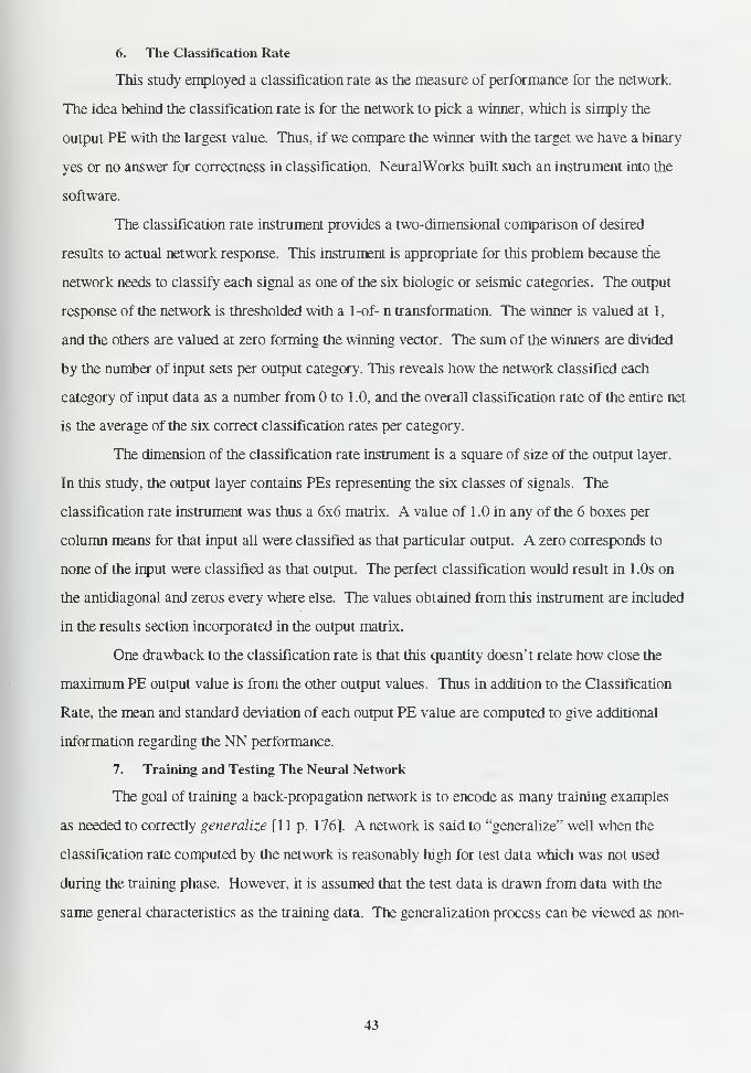
6. The Classification Rate

This study employed a classification rate as the measure of performance for the network.

The idea behind the classification rate is for the network to pick a winner, which is simply the

output PE with the largest value. Thus, if we compare the winner with the target we have a binary

yes or no answer for correctness in classification. NeuralWorks built such an instrument into the

software.

The classification rate instrument provides a two-dimensional comparison of desired

results to actual network response. This instrument is appropriate for this problem because the

network needs to classify each signal as one of the six biologic or seismic categories. The output

response of the network is thresholded with a 1-of- n transformation. The winner is valued at 1,

and the others are valued at zero forming the winning vector. The sum of the winners are divided

by the number of input sets per output category. This reveals how the network classified each

category of input data as a number from to 1 .0, and the overall classification rate of the entire net

is the average of the six correct classification rates per category.

The dimension of the classification rate instrument is a square of size of the output layer.

In this study, the output layer contains PEs representing the six classes of signals. The

classification rate instrument was thus a 6x6 matrix. A value of 1 .0 in any of the 6 boxes per

column means for that input all were classified as that particular output. A zero corresponds to

none of the input were classified as that output. The perfect classification would result in 1.0s on

the antidiagonal and zeros every where else. The values obtained from this instrument are included

in the results section incorporated in the output matrix.

One drawback to the classification rate is that this quantity doesn't relate how close the

maximum PE output value is from the other output values. Thus in addition to the Classification

Rate, the mean and standard deviation of each output PE value are computed to give additional

information regarding the NN performance.

7. Training and Testing The Neural Network

The goal of training a back-propagation network is to encode as many training examples

as needed to correctly generalize [lip. 176]. A network is said to "generalize" well when the

classification rate computed by the network is reasonably high for test data which was not used

during the training phase. However, it is assumed that the test data is drawn from data with the

same general characteristics as the training data. The generalization process can be viewed as non-

43

linear curve fitting, or a non-linear input-output mapping. This view point allows us to visualize

the learning process not as a 'magical life giving process' but as a good non-linear interpolation of

the data. A network that is designed well and is adequately trained should still have a high

classification rate when tested on data that is slightly different from the data used for training.

When the network learns too many ambiguous input-output relationships, that is, when it is

overtrained, the network may produce poor results even when tested with data that is only slightly

different from the testing set.

NeuralWorks provides a learning and testing scheme called Savebest to mitigate the effects

of overtraining. The option Savebest trains the network for a user prescribed number of epochs,

and tests the network with the testing file. The result is compared to the previous saved best

network. The network is saved based on the criteria, i.e., highest classification rate, or lowest root-

mean square error. This process repeats for the user prescribed number of failures to produce a

new best. The network when finished will revert to the saved-best network, thus averting an

overtrained network that memorizes the training set of data.

In this study, the length of training sets before testing is set at 10,000 epochs and the

number of retries, or failures to produce a new best, is set at 20. The criteria used was the overall

classification rate.

The training and testing files were built using the signals as described in the previous

chapters. Using MATLAB®, a matrix was constructed with each column representing the features.

For example, in the case of the reduced-rank covariance method, the number of features was the 25

model parameters per segment, in the case of the A-Trous algorithm with 4voices per octave, the

number of features was equal to 28 average energy values per voice and segment. The matrix was

appended with the target vector consisting of six values of either a one or a zero corresponding to

the output neuron designated to the classification of the data. The data was separated into training

files and testing files by using two thirds of the smallest file as the minimum number of training

files per class of data, which amounted to 86 files. The remaining one third, of the smallest

category was used as minimum number of testing files per class. Training files and testing files

were set up for each of the feature extraction methods. The features include reduced-rank

covariance(AR) coefficients, ALE pre-processed AR coefficients, wavelet average energy per

scale for both Symmlet 8, and Coiflet 3 coefficients, ALE pre-processed wavelet average energy

per scale for both Symmlet 8, and Coiflet 3 coefficients, AR and wavelet methods combined for

44

Symmlet and Coiflet coefficients, ALE pre-processed AR and wavelet combination for both

Symmlet and Coiflet coefficients, and finally the average energy per voice per scale using the A

Trous method for 3, 4,5,6, and 7 voices per octave. In all, 40 different networks were trained using

the fifteen above categories. The twelve best networks are presented in the results.

45

46

V. RESULTS

The top twelve NN implementations of all networks considered in this study are

summarized in Table 5.1. Note that ALE based noise reduction was not applied when using the A-

Trous implementation due to the high classification rate already achieved. The network numbers in

the second column of the table represent the number of PEs in the input layer/ hidden layer 1/

hidden layer 2/ and the output layer. The overall classification rate is as defined earlier in Chapter

IV section 6. In many of the feature extraction methods used, we tried toCi

clean" the signals by

applying the ALE algorithm to reduce the noise and increase the ability of the NN to classify the

signal. The last and second to last method used both the AR and Wavelet feature extraction

methods on the signal and combined the features into one vector for the NN to classify. The last

method took this approach one step further by using the ALE algorithm first.

Feature Extraction Method Network Overall Classification Rate

AR Coefficients 25/20/15/6 84.50 %ALE/AR Coefficients 25/20/15/6 83.94 %Wavelet (Coiflet 3) 14/14/10/6 78.05 %Wavelet (Symmlet 8) 14/14/10/6 84.67 %ALEAVavelet (Coiflet 3) 14/14/10/6 88.76 %ALE/Wavelet (Symmlet 8) 14/14/10/6 95.17 %A-Trous (4 Voices Per

Scale)

28/28/15/6 96.41 %

A-Trous (5 Voices Per

Scale)

35/20/15/6 93.46 %

A-Trous (6 Voices Per

Scale)

42/42/15/6 96.73 %

A-Trous (7 Voices Per

Scale)

49/49/15/6 95.10 %

AR & Wavelet (Coiflet 3) 39/30/15/6 86.64 %ALE/AR & Wavelet (Coiflet

3)

39/30/15/6 95.78 %

Table 5.1 Feature Extraction Performances

Table 5.1 shows that the highest scoring network is obtained for the A-Trous algorithm

with six voices per scale. The best solution, requiring the least preprocessing and the smallest

neural network, is, however the A-Trous algorithm with four voices per scale. Five networks

achieved an overall classification rate in excess of 95 %. This is our self induced threshold for a

47

successful classification scheme. Note that performance could potentially be farther improved by

optimizing the neural network for each feature extraction method.

Tables 5.2 to 5.13 and Figures 5.1 to 5.12 present the performances obtained with each of

the feature extraction methods summarized in table 5.1. For clarity purposes, a detailed

explanation of Table 5.2 is presented next. Tables 5.3 to 5. 13 follow the same presentation.

The 1st

row in Table 5.2 indicates the number of testing files presented to the NN for

classification in each class of signal. The 1st

column indicates the number of testing files classified

in a specific class. All other rows show the mean and standard deviation (STD) obtained at each

output node. The classification rate (CR) is as defined in Chapter IV section 6. Finally, the

number of files classified in each class of signal is included.

Row 2 to 6 present individual performance results obtained for each class. For example,

Row 2 shows that 56 files were classified as "Sperm Whale" data, and that 41 out of 5 1 files were

correctly classified, leading to a classification rate CR = 81%. Miss-classified sperm whale data

were classified as either killer whale (7 files) or earthquake files (3 files). In addition, average

output node levels are presented. For example, the average output level obtained for the Sperm

Whale output node when the NN is presented with Sperm Whale data is 0.6602, and its standard

deviation (STD) is equal to 0.3602. Note that the Sperm Whale output node level significantly

drops down to an average of 0.0656 when the NN is presented with other types of signals(as seen

across the top row), as expected. The main diagonal starting from the upper left of the table to the

lower right contains the number of correct classifications obtained for the testing data.

Performance results contained in Table 5.2 are also graphically presented in Figure 5.1. Class

number 1 through 6 refer to Sperm, Killer, Humpback, Gray, Pilot whales and earthquake data.

Test files 1 to 51 represent Sperm Whale data, Test files 52 through 102 represent Killer whale

data, test files 103 through 153 represent Humpback Whale test data, test files 153 through 204

represent Gray Whale data, test files 205 through 256 represent Pilot Whale data, and test files

257 through 306 represent earthquake data.

48

A. PERFORMANCE RESULTS OBTAINED USING REDUCED-RANK AR

COEFFICIENTS

1. No ALE Preprocessing

Figure 5.1 and Table 5.2 present the NN output classification results obtained using

reduced rank coefficients (AR).

Distribution of Neural Net Output File

»,(t

»*.JL

*:^M &$*""^-'l > <

1-

0.5-

0-

fvtl., i.>, >.. vj.

; , my it L

j

1 P-

U^5JLi

*i

50kj

"<4-i i'

100

150

200 Class

250

Test File Number300

Figure 5-1 Distribution of neural network classifications obtained using reduced-rank ARcoefficients. Overall classification rate: 84.50%.

The overall classification rate of 84.50 % is somewhat disappointing. However, note that

biological and earthquake AR frequency contents partially overlap. As a result, the NN has

difficulties classifying the data correctly.

49

Mean Sperm Killer Humpback Gray Pilot Earthquake

(STD) Input Input Input Input Input Input

CR% 51 files 51 files 51 files 51 files 51 files 51 files

306 files

Sperm 0.6602 0.2395 0.0295 0.0217 -0.0408 0.0781

Output(0.3602) (0.3010) (0.1746) (0.1717) (0.1790) (0.2457)

56 files81.00%

41 files

27.45 %

14 files

0% 0% 1.96%

1 file

0%

Killer 0.2389 0.8464 0.0240 -0.0393 -0.0550 -0.0171

Output (0.4447) (0.3054) (0.1102) (0.1380) (0.1119) (0.1240)

44 files 13.29 %

7 files

66.67 %

34 files

0% 5.71 %

3 files

0% 0%

Humpback 0.0072 -0.0571 0.9530 -0.0793 0.0319 0.0248

Output (0.0773) (0.1408) (0.1961) (0.0713) (0.0923) (0.1836)

52 files 0% 0% 94.29 %

48 files

0% 8.57%

4 files

0%

Gray -0.0374 0.0036 -0.0749 0.8942 0.0748 -0.0572

Output (0.1234) (0.2416) (0.0661) (0.3482) (0.2560) (0.0819)

49 files 0% 5.71 %

3 files

0% 85.71%

44 files

2.86 %

2 files

0%

Pilot 0.0241 -0.0649 -0.0413 0.0523 0.8328 -0.0437

Output (0.2179) (0.1101) (0.2079) (0.2271) (0.3427) (0.1661)

45 files 0% 0% 0% 8.57%

4 files

81.0%

41 files

0%

Earthquake -0.1020 -0.0356 0.0194 0.0018 0.0176 0.8972

Output (0.0220) (0.0177) (0.0655) (0.0362) (0.0245) (0.1012)

60 files 5.71% 0% 5.71 % 0% 5.71% 100%

3 files 3 files 3 files 51 files

Table 5.2 Distribution of neural network classifications obtained using reduced-rank ARcoefficients; overall classification rate: 84.5 %

50

2. ALE Preprocessing Applied to Data

Figure 5.2 and Table 5.3 present classification results obtained when the underwater data

is first pre-processed using the adaptive line enhancer (ALE) filter introduced earlier in Chapter III

section 3. This filter is applied to emphasize the narrow band contents contained in the data and

decrease wide-band noise. Next the reduced rank AR coefficients of the filtered data are computed

to be used as feature parameters. Note that the overall classification performance decreased. A

possible explanation is that the ALE step removes some of the unique AR- features of the signal,

thereby making it more difficult for the NN to classify the data correctly.

Distribution of Neural Net Output File

vV-'VA

-„ ., ...

-V-'V;;

Classification

Test File Number300

Figure 5-2 Distribution of neural network classifications obtained with reduced-rank ARcoefficients; ALE preprocessing applied to the data; overall classification rate: 83.94%.

51

MeanSperm Killer Humpback Gray Pilot Earthquake

Input Input Input Input Input Input

(STD)51 files 51 files 51 files 51 files 51 files 51 files

CR%

306 files

Sperm 0.3979 0.1095 0.0838 0.0809 0.1520 -0.0155

Output(0.3524) (0.1532) (0.1562) (0.1579) (0.2062) (0.0554)

63 files82.35 % 7.41 % 13.72 % 8.47 % 10.17% 0%

42 files 5 files 7 files 4 files 5 files

Killer -0.0001 0.8138 0.0037 -0.0427 0.1473 -0.0604

Output (0.1784) (0.3287) (0.1146) (0.0987) (0.1947) (0.0366)

57 files 4.0% 92.59 % 0% 11.86% 5% 0%

2 files 46 files 6 files 3 files

Humpback 0.0473 0.0067 0.7841 -0.0157 0.0906 0.0673

Output (0.1922) (0.0595) (0.2247) (0.0747) (0.0923) (0.1382)

46 files 0% 0% 81.48%

42 files

5.08 %

3 files

0% 1.5%

lfile

Gray 0.0649 0.0508 0.0699 0.6492 0.1864 -0.0390

Output (0.1873) (0.1513) (0.2319) (0.3482) (0.2634) (0.1047)

38 files 6%

3 files

0% 0% 69.49 %

35 files

0% 0%

Pilot 0.0225 0.0993 -0.0244 -0.0401 0.7254 0.0871

Output (0.1734) (0.1439) (0.0607) (0.0882) (0.3118) (0.0889)

53 files 8% 0% 1.85% 3.34 % 84.75 % 5%

4 files 1 file 2 files 43 files 3 files

Earthquake 0.1189 -0.0564 0.1523 0.0255 0.1421 0.6543

Output (0.1963) (0.0287) (0.1343) (0.0679) (0.1822) (0.2823)

49 files 0% 0% 1.85%

1 files

1.89%

lfile

0% 93%

47 files

Table 5.3 Distribution of neural network classifications obtained with reduced-rank ARcoefficients; ALE preprocessing applied to the data; overall classification rate: 83.94%.

52

B. CLASSIFICATION RESULTS OBTAINED WITH WAVELET-TYPE

PARAMETERS

1. Orthogonal Wavelet Decomposition

a. No ALE preprocessing:

This section presents results obtained for the classification scheme using

orthonormal wavelet-type quantities as NN inputs. The resulting classification rate is nearly

identical to that obtained with the reduced-rank AR method in the case of the Symmlet 8 basis set.

However, this wavelet-based method offers the advantage of requiring fewer NN input parameters.

Fourteen coefficients are used as compared to twenty-five coefficients for the reduced rank AR

method. For this reason, this method represents a better solution even though the overall

classification rate is the same. The results obtained using the Coiflet 3 basis set do not reach the

level obtained by the AR and the Symmlet 8 basis set. Detailed results are contained in Figure 5-3

and Table 5.4 for Symmlet 8 wavelet coefficients. Results for Coiflet 3 wavelet coefficients are

contained in Figure 5-4 and Table 5.5.

Distribution of Neural Net Output File

1-s0.5

i

—-.''••>. ;

trYe* ~<-v.

3 Mi ti

1 T*fri

Test File Number300

Figure 5-3 Distribution of neural network classifications obtained using the orthonormal wavelet

decomposition; Symmlet 8 basis set; overall classification rate: 84.67%.

53

MeanSperm Killer Humpback Gray Pilot Earthquake

Input Input Input Input Input Input

(STD)50 files 50 files 50 files 50 files 50 files 50 files

CR%

300 files

Sperm 0.8362 0.1897 -0.0362 0.0417 -0.0590 -0.0154

Output(0.2347) (0.2012) (0.0334) (0.1776) (0.0716) (0.0381)

62 files92.00 %

46 files

22%

11 files

0% 10%

5 files

0% 0%

Killer 0.1990 0.6077 0.0042 0.0844 -0.0039 -0.0392

Output (0.2662) (0.3677) (0.0842) (0.2198) (0.1077) (0.0526)

46 files 4.0%

2 files

66%

33 files

0% 22%

11 files

0% 0%

Humpback -0.0330 0.0050 0.9086 -0.0008 -0.0278 0.0566

Output (0.0451) (0.1858) (0.2236) (0.0342) (0.0757) (0.2145)

46 files 0% 0% 92%

46 files

0% 0% 0%

Gray 0.0926 0.2735 0.0056 0.4547 0.0996 0.0097

Output (0.2294) (0.1955) (0.0339) (0.2418) (0.2053) (0.1499)

41 files 4% 12% 0% 62% 4% 0%

2 files 6 files 31 files 2 files

Pilot -0.1071 -0.0576 -0.0124 0.1022 0.9957 -0.0073

Output (0.0213) (0.0826) (0.0385) (0.1670) (0.1474) (0.0776)

50 files 0% 0% 0% 4%

2 files

96%

48 files

0%

Earthquake -0.0188 -0.0151 -0.0114 -0.0306 -0.0135 1.0203

Output (0.0522) (0.0558) (0.0337) (0.0630) (0.0603) (0.1275)

55 files 0% 0% 8%

4 files

2%

1 file

0% 100%

50 files

Table 5.4 Distribution of neural network classifications obtained using the orthonormal wavelet

decomposition; Symmlet 8 basis set; overall classification rate: 84.67%.

54

Figure 5-4 and Table 5.5 below displays the results of using Coiflet 3 basis set. This

feature extraction technique achieved an overall classification of 78.05%. The results are

disappointing in that they are far below that obtained by using the Symmlet 8 basis set and the AR

neural networks.

Distribution of Neural Net Output File

:'<*• '•'.

'""--•*..> .-.,

'' 'y. nil

Class

Test File Number300

Figure 5-4 Distribution of neural network classifications obtained using the orthonormal wavelet

decomposition; Coiflet 3 basis set; overall classification rate: 78.05%.

55

MeanSperm Killer Humpback Gray Pilot Earthquake

Input Input Input Input Input Input

(STD)50 files 50 files 50 files 50 files 50 files 50 files

CR%

300 files

Sperm 0.7850 0.3198 -0.0115 -0.0160 -0.0060 0.0081

Output(0.3072) (0.3488) (0.0521) (0.1398) (0.0600) (0.1042)

62 files70.73 %

35 files

4.88 %

2 files

0% 4.88%

2 files

0% 0%

Killer 0.0574 0.6608 0.0150 0.1068 -0.0202 -0.0687

Output (0.2515) (0.2676) (0.1278) (0.2627) (0.0790) (0.0521)

46 files 24.39 % 75.66 % 0% 9.76 % 4.88 % 0%

12 files 38 files 5 files 2 files

Humpback 0.0147 -0.0006 0.9148 -0.0430 -0.0214 0.0329

Output (0.0429) (0.0314) (0.1766) (0.0404) (0.0312) (0.2048)

44 files 0% 0% 90.24 %

45 files

0% 2.44%

lfile

14.63 %

7 files

Gray -0.0283 0.2779 -0.0156 0.4648 0.2288 -0.0169

Output (0.2111) (0.1766) (0.0846) (0.1816) (0.2253) (0.0323)

41 files 4.88 % 14.63 % 0% 65.85 % 12.20% 0%

2 files 7 files 33 files 6 files

Pilot -0.0882 0.0734 -0.0405 0.1257 0.7497 -0.0571

Output (0.0578) (0.2282) (0.1217) (0.2334) (0.3376) (0.0545)

52 files 0% 4.88 %

2 files

0% 19.51%

10 files

80.49%

40 files

0%

Earthquake -0.0560 -0.0548 -0.1087 -0.0925 0.0601 0.8384

Output (0.0553) (0.0727) (0.0258) (0.0492) (0.1589) (0.3723)

55 files 0% 0% 9.76 %

5 files

0% 0% 85.37 %

43 files

Table 5.5 Distribution of neural network classifications obtained using the orthonormal wavelet

decomposition; Coiflet 3 basis set; overall classification rate: 78.05%.

56

b. ALE pre-processing applied to data

This section presents classification results obtained when applying the ALE noise

reduction technique to the data before using Mallat's algorithm. In contrast to the AR process, the

multiresolution algorithm greatly benefited from the ALE pre-processing. The classification rate is

up to 95.17% for the Symmlet 8 basis set. Both the Symmlet 8 basis set and the Coiflet 3 basis set

increased the overall classification rate by ten percent by first pre-processing with the ALE filter.

Detailed results are presented in Figure 5-5 and Table 5.6 for the Symmlet 8 basis set next. Figure

5-6 and Table 5-7 present the data for Coiflet 3 basis set.

Distribution of Neural Net Output File

1-

0.5-

0-

i

>:~~.. vvv».'-—US*. I :«y .

».-*. At. ~-'-^.i

tr\

"^Tr-'s.

Test File Number300

Figure 5-5 Distribution of neural network classifications obtained using the orthonormal wavelet

decomposition; Symmlet 8 basis set; ALE pre-processing; overall classification rate: 95.17%.

57

MeanSperm Killer Humpback Gray Pilot Earthquake

Input Input Input Input Input Input

(STD)50 files 50 files 50 files 50 files 50 files 50 files

CR%

300 files

Sperm 1.0113 0.0238 -0.0653 0.0457 -0.0855 -0.0875

Output(0.1409) (0.1085) (0.0371) (0.0989) (0.0442) (0.0440)

52 files 100%

50 files

2.44%

1 file

0% 2.44%

lfile

0% 0%

Killer 0.0437 0.6672 0.0192 0.2334 -0.0288 -0.0301

Output (0.1719) (0.2955) (0.0643) (0.2948) (0.0862) (0.0273)

49 files 0% 93.00 %

46 files

0% 4.92 %

3 files

0% 0%

Humpback -0.0214 0.1878 0.7800 0.0051 -0.0720 0.0274

Output (0.0423) (0.4440) (0.3461) (0.1172) (0.0578) (0.1969)

50 files 0% 0% 100%

50 files

0% 0% 0%

Gray -0.0349 0.2912 0.0163 0.6332 0.0480 0.0119

Output (0.1216) (0.1831) (0.0564) (0.1980) (0.1048) (0.0410)

54 files 0% 4.92 %

3 files

0% 90.24 %

45 files

12.2 %

6 files

0%

Pilot -0.0646 -0.0823 -0.0357 0.0975 0.9516 -0.0008

Output (0.0603) (0.0267) (0.0534) (0.1189) (0.1642) (0.0554)

45 files 0% 0% 0% 2.00%

1 file

87.8%

44 files

0%

Earthquake -0.0543 -0.0172 -0.0925 -0.0683 0.0324 0.9928

Output (0.0490) (0.0648) (0.0306) (0.0325) (0.1420) (0.2728)

50 files 0% 0% 0% 0% 0% 100%

50 files

Table 5.6 Distribution of neural network classifications obtained using the orthonormal wavelet

decomposition; Symmlet 8 basis set; ALE pre-processing; overall classification rate: 95.17%.

58

Figure 5-6 and Table 5.7 display the results of the ALE Coiflet 3 basis set. The overall

classification rate of 88.75% is a drastic improvement over the Coiflet 3 set alone, however it does

not quite match the 95. 17% achieved by the ALE Symmlet 8 basis set. It is an improvement over

the AR coefficient method and did require a smaller neural network to implement. In this respect,

it is a more successful implementation. It does not meet the 95% self induced threshold for

success.

Distribution of Neural Net Output File

?%....*

w„

'Z'J^KJ: ;TV^

T* ~p

f\i\ J "\ -NT-

ir

Hvv<»

Test File Number300

Class

Figure 5-6 Distribution of neural network classifications obtained using the orthonormal wavelet

decomposition; Coiflet 3 basis set; ALE pre-processing; overall classification rate: 88.75%

59

MeanSperm Killer Humpback Gray Pilot Earthquake

Input Input Input Input Input Input

(STD)50 files 50 files 50 files 50 files 50 files 50 files

CR%

300 files

Sperm 1.0042 0.0120 -0.0668 0.0558 -0.0735 -0.0770

Output(0.1352) (0.0904) (0.0377) (0.0931) (0.0583) (0.0528)

52 files100%

50 files

2.44%

1 file

0% 2.44%

lfile

0% 0%

Killer 0.0347 0.6648 0.0108 0.2261 -0.0309 -0.0260

Output (0.1454) (0.3018) (0.0543) (0.3018) (0.0604) (0.0282)

34 files 0% 62.79 %

31 files

0% 6.98 %

3 files

0% 0%

Humpback 0.0238 -0.1070 1.0822 0.0067 -0.0914 -0.0213

Output (0.0279) (0.0270) (0.0285) (0.0161) (0.0226) (0.0245)

50 files 0% 0% 100%

50 files

0% 0% 0%

Gray -0.0346 0.2996 0.0101 0.6301 0.0517 0.0345

Output (0.1103) (0.1159) (0.0205) (0.1700) (0.1380) (0.1492)

59 files 0% 34.88 %

17 files

0% 83.72 %

42 files

0% 0%

Pilot -0.0537 -0.0774 -0.0342 0.0835 0.9490 0.0431

Output (0.0867) (0.0496) (0.0558) (0.1255) (0.1704) (0.1802)

59 files 0% 0% 0% 4.88%

2 files

100%

50 files

13.95 %

7 files

Earthquake -0.0515 -0.0308 -0.0663 -0.0339 0.0593 0.8279

Output (0.0616) (0.0671) (0.0688) (0.0573) (0.1360) (0.3999)

44 files 0% 0% 0% 2.44%

1 file

0% 86.05 %

43 files

Table 5.7 Distribution of neural network classifications obtained using the orthonormal wavelet

decomposition; Coiflet 3 basis set; ALE pre-processing; overall classification rate: 88.75%.

60

2. Non-Orthogonal A-Trous Wavelet Decomposition

This section presents classification results obtained when applying the A-Trous algorithm.

Note the ALE noise reduction technique is not applied to the data as the performance is

satisfactory without it. The A-Trous algorithm takes advantage of a better frequency resolution

obtained when using multiple voices. Results show that classification performance is improved

using this method as compared to the other methods used in this study.

The A-Trous decomposition is implemented with four different combinations of voices.

Four, five, six, and seven voices per scale are presented. Results show that the overall best

classification rate is obtained when using six voices per scale, however the size of the NN was

significantly larger. Figures 5-7 through 5-10 and Tables 5.8 through 5.11 present the

performance results.

V

a. A-Trous Implementation with four voices per scale

Distribution of Neural Net Output File

: ' < l?i

"•VWJfc

JMA

A,

->-u, rtr^i

-HAS h

- 6

Test File Number300

Figure 5-7 Distribution of neural network classifications obtained using the A-Trous

implementation; 4 voices per scale; overall classification rate: 96.41%.

61

Mean Sperm Killer Humpback Gray Pilot Earthquake

(STD) Input Input Input Input Input Input

CR% 51 files 51 files 51 files 51 files 51 files 51 files

306 files

Sperm 1.1055 -0.1058 0.1253 -0.0932 0.2603 -0.0588

Output (0.0768) (0.0803) (0.2209) (0.1125) (0.2989) (0.0481)

51 files 98.04 %

50 files

1.96%

1 file

0% 0% 0% 0%

Killer -0.0279 0.8835 -0.0578 -0.0378 0.0317 -0.0599

Output (0.2152) (0.2500) (0.1303) (0.1090) (0.2125) (0.1133)

46 files 0% 90.20 %

46 files

0% 0% 0% 0%

Humpback -0.0081 0.0571 1.0518 -0.0086 -0.0540 0.1096

Output (0.0680) (0.1544) (0.1287) (0.0826) (0.0655) (0.1198)

51 files 0% 0% 100%

51 files

0% 0% 0%

Gray -0.0709 -0.0566 -0.1007 1.0186 -0.0055 0.0018

Output (0.0672) (0.0845) (0.0424) (0.1749) (0.1646) (0.1737)

53 files 0% 0% 0% 98.04 %

50 files

5.88 %

3 files

0%

Pilot 0.0668 -0.0250 0.0008 0.1808 0.7893 -0.0273

Output (0.1091) (0.0857) (0.0876) (0.1753) (0.2384) (0.1775)

52 files 1.96%

1 file

7.84 %

4 files

0% 0% 92.16%

47 files

0%

Earthquake -0.0799 -0.0862 -0.1247 0.0248 0.2086 1.0175

Output (0.0371) (0.0699) (0.0009) (0.1136) (0.2744) (0.2166)

53 files 0% 0% 0% 1.96%

1 file

1.96%

lfile

100%

51 files

Table 5.8 Distribution of the neural network classifications obtained using the A-Trous

implementation; 4 voices per scale; overall classification rate: 96.41%

62

b. A-Trous Implementation with five voices per scale

Figure 5.8 and Table 5.9 display the results obtained from 5 voices pre scale.

Note that the resultant overall classification rate is less than that obtained from four voices per

scale. This was not expected. The expectation was that an increase in resolution of the feature

extraction would produce an increase in the overall classification rate.

Distribution of Neural Net Output File

»*s, •

telit ft.*-.

**

—

z*Vw ] u^s>~'v*i W \. \t\—^>rA i H

Test File Number300

Figure 5-8 Distribution of neural network classifications obtained using the A-Trous

implementation; 5 voices per scale; overall classification rate: 93.46 %.

63

MeanSperm Killer Humpback Gray Pilot Earthquake

Input Input Input Input Input Input

(STD)51 files 51 files 51 files 51 files 51 files 51 files

CR. %

306 files

Sperm 1.0772 -0.0993 0.1176 -0.1176 0.2158 -0.0244

Output (0.1719 (0.0937) (0.1915) (0.0225) (0.2746) (0.0847)

50 files 98.04 %

50 files

0% 0% 0% 0% 0% •

Killer -0.0241 0.8539 -0.0205 0.0344 0.0585 -0.0349

Output (0.2131) (0.2843) (0.1391) (0.2557) (0.2295) (0.0497)

50 files 0% 86.27 %

44 files

0% 5.88 %

3 files

1.96%

1 files

0%

Humpback 0.1622 -0.0119 1.0302 0.0658 0.0883 0.0450

Output (0.3230) (0.0822) (0.2397) (0.2254) (0.2702) (0.1794)

49 files 0% 0% 96.08 %

49 files

0% 1.96%

lfile

0%

Gray -0.0877 0.0312 -0.0973 0.8953 -0.0364 0.0257

Output (0.0376) (0.2181) (0.0332) (0.3045) (0.1775) (0.1469)

53 files 0% 11.76%

6 files

0% 92.16 %

47 files

7.84 %

4 files

0%

Pilot -0.0437 -0.0075 0.0159 0.0592 0.7276 0.0036

Output (0.1527) (0.1035) (0.0980) (0.1890) (0.3100) (0.0991)

51 files 1.96% 1.96% 0% 1.96% 88.24 % 0%

1 file 1 files 1 files 45 files

Earthquake -0.0660 -0.1115 -0.1215 0.0119 0.2458 1.0710

Output (0.0500) (0.0310) (0.0076) (0.1349) (0.3796) (0.0951)

53 files 0% 0% 3.92 %

2 files

0% 0% 100%

51 files

Table 5.9 Distribution of the neural network classifications obtained using the A-Trous

implementation; 5 voices per scale; overall classification rate: 93.46 %

64

c. A-Trous Implementation with six voices per scale

This implementation of the A-Trous algorithm has the highest classification rate of

all tested. Even though this implementation has the overall best classification rate, it also has more

false earthquake classifications than either four voices or five voices per scale. In addition it

requires a higher number of NN input coefficients and correspondingly a more complex NN.

Distribution of Neural Net Output File

ply IA

TtfeJ^VJI V

^nr«_ ^--- :l•'

::~

—

:

1

Test File Number300

Figure 5-9 Distribution of the neural network classifications obtained using the A-Trous

implementation; 6 voices per scale; overall classification rate: 96.73%.

65

MeanSperm Killer Humpback Gray Pilot Earthquake

Input Input Input Input Input Input

(STD)51 files 51 files 51 files 51 files 51 files 51 files

CR%

306 files

Sperm 1.1107 -0.0848 0.1438 -0.1224 0.2516 -0.0579

Output(0.0751) (0.1879) (0.0100) (0.3110) (0.0670) (0.0481)

50 files98.04 %

50 files

0% 0% 0% 0% 0%

Killer -0.0735 0.9539 0.0807 -0.0271 -0.0321 -0.0340

Output (0.1462) (0.2745) (0.1903) (0.1585) (0.0450) (0.1133)

51 files 0% 98.04 %

50 files

0% 1.96%

1 file

0% 0%

Humpback -0.0468 0.2230 1.0638 0.0304 -0.0205 0.0399

Output (0.0856) (0.2996) (0.1425) (0.1423) (0.1759) (0.1198)

49 files 0% 0% 96.08 %

49 files

0% 0% 0%

Gray -0.0916 0.0776 -0.1028 0.9014 -0.0263 0.0083

Output (0.0480) (0.3277) (0.3471) (0.1959) (0.1633) (0.1737)

52 files 0% 0% 0% 96.08 %

49 files

5.88 %

3 files

0%

Pilot 0.0221 -0.0585 0.0136 0.0238 0.8450 -0.0198

Output (0.2134) (0.0892) (0.2466) (0.3758) (0.1460) (0.1775)

48 files 1.96%

1 file

1.96%

1 file

0% 0% 92.16%

46 files

0%

Earthquake -0.1000 -0.1159 -0.1233 0.1588 0.1851 1.0276

Output (0.0249) (0.0198) (0.2570) (0.3106) (0.1454) (0.2166)

55 files 0% 0% 3.92 % 1.96% 1.96% 100%

2 files 1 file 1 file 51 files

Table 5.10 Distribution of the neural network classifications obtained using the A-Trous

implementation; 6 voices per scale; overall classification rate: 96.73 %.

66

d. A-Trous Implementation with seven voices per scale

Results show an overall classification rate of 95. 10%, as indicated earlier in Table

5.1. Note that the NN implementation complexity has increased due to the larger number of input

NN coefficients. This NN configuration has 49 PEs in the input layer, 49 PEs in hidden 1,15 PEs

in hidden 2, and 6 output PEs. This is the largest network considered in this study. Figure 5-10 and

Table 5.11 present classification results obtained using the set of averaged wavelet-type

coefficients. We note that the NN implementation obtained with four voices per scale has a better

overall classification rate using a much smaller network.

Distribution of Neural Net Output File

fmnrvt{:™N~,

*^*.

I*. ; 3..:

r%&^rvJW

Class

Test File Number300

Figure 5-10 distribution of neural network classifications obtained using the A-Trous

implementation: 7 voices per scale; overall classification rate: 95.10 %.

67

MeanSperm Killer Humpback Gray Pilot Earthquake

Input Input Input Input Input Input

(STD)51 files 51 files 51 files 51 files 51 files 51 files

CR%

306 files

Sperm 1.1107 -0.0848 0.1438 -0.1224 0.2516 -0.0579

Output(0.0751) (0.1879) (0.0100) (0.3110) (0.0670) (0.0481)

51 files100%

51 files

0% 0% 0% 0% 0%

Killer -0.0735 0.9539 0.0807 -0.0271 -0.0321 -0.0340

Output (0.1462) (0.2745) (0.1903) (0.1585) (0.0450) (0.1133)

57 files 0% 98.04 %

50 files

0% 13.73 %

7 files

0% 0%

Humpback -0.0468 0.2230 1.0638 0.0304 -0.0205 0.0399

Output (0.0856) (0.2996) (0.1425) (0.1423) (0.1759) (0.1198)

50 files 0% 0% 98.04 %

50 files

0% 0% 0%

Gray -0.0916 0.0776 -0.1028 0.9014 -0.0263 0.0083

Output (0.0480) (0.3277) (0.3471) (0.1959) (0.1633) (0.1737)

49 files 0% 1.96%

lfile

0% 84.31 %

43 files

9.80 %

5 files

0%

Pilot 0.0221 -0.0585 0.0136 0.0238 0.8450 -0.0198

Output (0.2134) (0.0892) (0.2466) (0.3758) (0.1460) (0.1775)

47 files 0% 0% 0% 1.96%

lfile

90.20 %

46 files

0%

Earthquake -0.1000 -0.1159 -0.1233 0.1588 0.1851 1.0276

Output (0.0249) (0.0198) (0.2570) (0.3106) (0.1454) (0.2166)

52 files 0% 0% 1.96%

1 file

0% 0% 100%

51 files

Table 5.11 Distribution of neural network classifications obtained using the A-Trous

implementation: 7 voices per scale; overall classification rate: 95.10 %.

68

C. CLASSIFICATION RESULTS OBTAINED BY COMBINING AR

COEFFICIENTS AND ORTHONORMAL WAVELET-TYPE PARAMETERS

This section presents classification results obtained by combining the ALE AR and

wavelet feature coefficients. This technique is considered in this study to investigate the results

when a combination of dissimilar approaches is applied. The premise behind this approach is the

combination of different techniques would provide unique combinations of parameters for input

into the NN. The combination may dramatically increase the classification rate over any single

technique applied alone. It is the most labor intensive pre-processing technique applied in this

study, and requires a large, complex neural network.

1. No ALE Pre-processing Applied to the Data

Figure 5-9 and Table 5.10 present the results obtained by combining the reduced-rank

coefficients with wavelet - type parameters using the Coiflet 3 basis set. Redundant processing

with different techniques should produce better results than either technique alone. This technique

only slightly enhanced the classification rate of either alone.

Distribution of Neural Net Output File

: 2

Class

Test File Number300

Figure 5-11 Distribution of neural network classifications obtained using the combination of

reduced-rank AR coefficients and wavelet-type techniques; Coiflet 3 basis set; overall classification

rate: 86.64%.

69

MeanSperm Killer Humpback Gray Pilot Earthquake

Input Input Input Input Input Input

(STD)50 files 50 files

.

50 files 50 files 50 files 50 files

CR%

300 files

Sperm 0.8461 0.1606 -0.0659 -0.0061 -0.0896 -0.0449

Output(0.2763) (0.1659) (0.0529) (0.0842) (0.0460) (0.0233)

53 files87.80 %

44 files

17.07 %

9 files

0% 0% 0% 0%

Killer 0.1645 0.5969 -0.0847 0.0968 -0.0699 -0.0622

Output (0.2900) (0.3959) (0.0369) (0.2703) (0.0715) (0.0374)

39 files9.76 % 56.10% 0% 9.76 % 2.00 % 0%

5 files 28 files 5 files 1 file

Humpback -0.0599 -0.1201 1.0559 0.0145 -0.1131 0.1199

Output (0.0521) (0.0112) (0.1703) (0.1015) (0.0203) (0.1784)

49 files 0% 0% 98.00 %

49 files

0% 0% 0%

Gray 0.0728 0.0736 -0.0933 0.6169 0.0338 0.0314

Output • (0.2474) (0.1374) (0.0355) (0.2902) (0.1887) (0.0767)

61 files 2.00 % 26.00 % 0% 87.80 % 4.88 % 0%

1 file 13 files 44 files 3 files

Pilot -0.0588 0.0083 -0.0897 0.0631 0.8373 0.0065

Output (0.0635) (0.1818) (0.0417) (0.2117) (0.3109) (0.1939)

46 files 0% 0% 0% 2.44%

1 file

90.24 %

45 files

0%

Earthquake -0.0510 -0.0574 -0.1120 -0.0380 0.0266 1.0388

Output (0.0602) (0.0525) (0.0095) (0.0344) (0.0494) (0.1326)

52 files 0% 0% 2.00 %

1 file

0% 2.00 %

1 file

100%

50 files

Table 5.12 Distribution of neural network classifications obtained using the combination of reduced-

rank AR coefficients and wavelet-type parameters; Coiflet 3 basis set; overall classification rate:

86.64%.

70

2. ALE Pre-processing Applied to the Data

Figure 5-12 and Table 5.13 present the results obtained by first pre-processing the data

using an ALE filter and next computing reduced-rank AR coefficients in combination with wavelet-

type parameters. It produced an overall classification rate of 95.78 %. The results are impressive

however, they came at the cost of pre-processing time and a very complex neural network.

Distribution of Neural Net Output File

^vS f\

-<Sr** '"*^L,4 «**.

VJ*.*^\,Ja

vv.

fc>Cr*J"H >?r

Test File Number300

Figure 5-12 Distribution of neural network classifications obtained using the combination of ALEpre-processing, reduced-rank AR coefficients, and wavelet-type parameters; Coiflet 3 basis set;

overall classification rate: 95.78 %

71

MeanSperm Killer Humpback Gray Pilot Earthquake

Input Input Input Input Input Input

(STD)50 files 50 files 50 files 50 files 50 files 50 files

CR%

300 files

Sperm 1.0952 -0.0983 -0.0070 0.0314 -0.0933 0.0704

Output(0.0771) (0.0363) (0.0805) (0.1403) (0.0336) (0.1420)

54 files100%

50 files

0% 0% 7.32 %

4 files

0% 0%

Killer -0.0201 0.9231 -0.0431 0.0231 -0.0013 -0.0960

Output (0.1889) (0.2554) (0.0627) (0.1948) (0.1276) (0.0313)

49 files 0% 92.10%

46 files

2.00 %

lfile

4.88 %

2 files

0% 0%

Humpback -0.0190 -0.0311 1.0365 0.0041 -0.0207 0.0264

Output (0.0750) (0.0517) (0.2427) (0.0776) (0.1113) (0.1517)

48 files 0% 0% 96.00 %

48 files

0% 0% 0%

Gray -0.0313 0.1827 -0.0508 0.7570 -0.0581 0.0358

Output (0.1497) (0.1662) (0.0481) (0.2290) (0.1476) (0.1704)

47 files 0% 7.80 %

4 files

0% 86.00 %

43 files

0% 0%

Pilot -0.0598 -0.0792 -0.0163 0.0622 1.0204 0.1038

Output (0.1699) (0.0574) (0.1071) (0.1890) (0.1904) (0.2787)

51 files 0% 0% 0% 2.00 %

lfile

100%

50 files

0%

Earthquake -0.0920 -0.0602 -0.1021 -0.0459 0.0298 0.9372

Output (0.0379) (0.0708) (0.0481) (0.0409) (0.2530) (0.1827)

51 files 0% 0% 2.00 %

lfile

0% 0% 100%

50 files

Table 5.13 Distribution of neural network classifications obtained using the combination of ALEpre-processing, reduced rank AR coefficients, and wavelet-type parameters; Coiflet 3 basis set;

overall classification rate: 95.78%.

72

VI. CONCLUSION AND RECOMMENDATIONS

A. CONCLUSION

This thesis investigated spectral based feature extraction techniques to input into a back-

propagation neural network to resolve ocean biologic signals from those produced by earthquakes.

The back-propagation neural network proved to be a very successful means of classifying the six

categories of signals when used in conjunction with a good feature extraction technique. This

thesis implemented a neural network classifier that can differentiate between earthquakes and five

different species of whale with an overall classification rate exceeding 95 %. Specifically

investigated were: 2 categories of feature extraction techniques, reduced-rank auto-regressive

modeling and discrete wavelet transform based techniques. An adaptive line enhancer was

investigated to improve the neural network results by removing uncorrelated noise. The specific

results for the AR modeling, the discrete wavelet transform using Symmlet 8 and Coiflet 3 wavelet

transforms, combining AR and DWT techniques, and finally the discrete wavelet transform using

an A Trous method are summarized in the following paragraphs.

The reduced-rank covariance method is used to produce AR models of the time domain

signals. The choice of model number was determined systematically using three model order

prediction techniques as discussed in Chapter III. The determination of usable singular values in

the algorithm is determined visually, which proved to be only moderately successful. The

combination of applying the ALE and using the reduced-rank covariance method produced results

that were actually worse than using the reduced rank method alone. The most successful neural

network implementation using this feature extraction technique had an overall classification rate of

84.67 % as reported in Chapter V.

Two implementations of the Wavelet Transform were considered; the Mallafs algorithm,

and the A-Trous algorithm. Mallat's algorithm computes an orthonormal decomposition. This

technique produced only moderately successful results on par with the reduced rank AR technique.

The combination of applying the ALE and using the orthonormal wavelet based technique was

somewhat more successful, however still not producing acceptable results. Investigated were

Symmlet 8 and Coiflet 3 wavelet families. Without ALE pre-processing the neural network overall

classification rates obtained were 84.67% and 78.05%. Using the ALE pre-processing, the results

were brought up to 95. 17% using the Symmlet 8 basis set. The Coiflet 3 basis set improved to

73

88.76%. Of note is the Symmlet 8 results are on par with the AR modeling technique with NN that

are two thirds the size of using AR modeling.

A combination of reduced-rank and orthonormal wavelet based techniques were

investigated. The premise being that by combining the two techniques, a unique paring of the two

methods would produce better results. The combination produced an overall classification rate of

86.58%. Only a slight improvement was realized over either technique alone. This combination

proved to be very successful when the ALE was also employed. An overall classification rate of

95.78% was achieved. This level of processing for the feature extraction is very labor intensive,

and involved using a large NN to classify the signals.

The A-Trous based technique lead to the best performing technique considered in this

study. This technique produced consistently highly successful results that did not need

augmentation with a noise reduction technique. Two of the three highest classification rates were

produced by neural networks implementing this technique. Three of the four NNs presented using

this technique were above 95% in the overall classification rate. The technique that combined a

high overall classification rate and a small NN is the A Trous with 4 voices per scale. The overall

classification rate achieved was 96.41% with a network only slightly larger than that used for the

AR modeling technique. Only one other extraction technique had a better overall classification rate,

the A Trous with 6 voices per scale. The increase in resolution came at the expense of a very large

NN and thus is not the optimal answer.

The back-propagation neural network proved to be a very successful means of classifying

the six categories of signals when used in conjunction with a good feature extraction technique.

The high rate of success was achieved even though very tittle effort was made to optimize the

neural networks for the data. Better results might be achieved by optimizing the neural network

architectures for each feature extraction technique. Improvements may also be realized by

employing a more sophisticated means of noise reduction.

74

B. RECOMMENDATIONS

High classification rates obtained using the non-orthogonal wavelet based techniques are

encouraging and warrant further study regarding the optimization of the NN implementation.

The lack of success of the AR method may be indicative of the relative simplistic

algorithm used in this study. ARMA modeling may provide a better solution while achieving a

reduction in the order of the model. A potential improvement of the reduced-rank covariance

technique would be to automate self adjusting of the number of singular values chosen. The visual

technique employed in this thesis was cumbersome and requires human intervention.

In addition, an improvement in the de-noising algorithm may be achieved by employing a

wavelet based de-noising technique suggested in [7]. The implementation of the ALE algorithm

was hampered by applying the same technique to all signals. The application ofa single technique

did not provide the optimum de-noising solution to any of the signals, yet provided an engineering

solution to de-noise the signals while not significantly degrading any single class of signal.

Wavelet based techniques may enhance the ability to de-noise live ocean signals better than the

ALE algorithm.

Finally, improvement could be obtained by employing a neural network architecture that is

capable of expanding to recognize new class of signals without having to be retrained on the

signals it already recognizes. One such architecture that shows promise is the Fuzzy ARTMAP

architecture mentioned in [10].

75

76

APPENDIX

ORDER.Mfunction [AIC,CAT,FPE.MDL,var]=order(data,P)

% ORDER uses the AIC, CAT, FPE, and MDL criteria to choose the

% appropriate AR model order. Each output variable is a P-by-1 vector

% with the quantities indicated. The index of the minimum of each quantity

% is the best theoretical model order. The variable "var" does not

% yield a minimum at the ideal model order; its usefulness is in examining

% the model order at which the variance becomes "flat."

%% Usage: [AIC,CAT,FPE,MDL,var]=order(data,P)

%% Input: data Sequence to be modeled

% P Highest model order to test (all model orders from

% 1 to P will be tested).

%% Output: AIC AIC quantity (vector of length P)

% CAT CAT quantity (vector of length P)

% FPE FPE quantity (vector of length P)

% MDL MDL quantity (vector of length P)

% var Theoretical prediction error variance (vector of length P)

%% ORDER calls the function BURG_A

% Written by K. L. Frack Last Update: 16 March 1994

Ns=length(data);

AIC=zeros(P,l);

CAT=zeros(P.l);

FPE=zeros(P,l);

MDL=zeros(P,l);

var=zeros(P,l);

forp=l:P;

[a,var(p)]=burg_a(data,p); % Compute variance at each order

AIC(p)=Ns*log(var(p))+2*p; % Compute AIC quantity

SUM=0;for pp=l:p %l Compute CAT quantity

SUM=SUM+(Ns-pp)/Ns/var(pp);

end

CAT(p)=SUM/Ns-(Ns-p)/Ns/var(p);

FPE(p)=var(p)*(Ns+p+l)/(Ns-p-l); % Compute FPE quantity

MDL(p)=Ns*log(var(p))+p*log(Ns); % Compute MDL quantity

end

77

BURG_A.Mfunction [a,var]= burg_a(data,P)

% Burg's Method AR Model

%% This function solves the AR model coefficients for the given data sequence

% using Burg's method.

%% Usage: [a,var] = burg_a(data,P)

%% Input: data Data sequence

% P Desired model order

%% Output: a Vector with "a" parameters ([1 al a2 ... aP])

% var Prediction error variance

% Written by K. L. Frack Last Update: 15 March 1994

[drow dcol]=size(data);

if dcol > 1 %l Ensures the data is a column vector

data=data';

end

N=length(data);

ef=data(2:N); % Initial forward prediction error vector

eb=data(l:N-l); % Initial backward prediction error vector

a=[l]; % Initial "a" vector

var=data'*data/N; % Initial error variance

fork=l:P

L=length(ef);

gam(k)=(2*ef *eb)/(ef *ef+eb'*eb); %l Burg's algorithm performed for

tef=ef(2:L)-conj(gam(k))*eb(2:L); %\ each of the p iterations

eb=eb(l:L-l)-gam(k)*ef(l:L-l);

ef=tef;

a=[a; 0]-conj(gam(k))*[0; flipud(conj(a))]; % update "a" vector

var=var*(l-abs(gam(k))A2); % Update error variance

end

ARWHALE.M

function [aw]=arwhale(q)

% AR model of signal q using the reduced-rank covariance method

% method reduces rank of estimared correlation matrix using the singular value decomposition

% User visully picks number of singular values to keep program plots FFT ofsignal vs frequency responce

% of AR model of segment

% Returns matrix of a coefficients for model segments [25 X number of segments]

% Written by LT R.C.Bennett, USN.

% ref ar_covar.m by LT D.Brown USN%% last modified 90ct94

n=[l:512]';

fs=l;

findex= 1:5 12/2;

78

freq=findex*fs/512;

Mo=25; %%%% model order

%%% data is a multiple of 512 segments

numseg=(floor(length(q)/512)); %%% number of segments

disp([' the number of segments are \num2str(numseg)])

aw=zeros(Mo+ 1 ,numseg);

for seg=l:numseg %% recursion to go through all

%% segments of one "whistle"

disp(['segment '.num2str(seg)]);

%%%%%%%%%%%segment=q((seg*512)-511:(seg*512));

%%%%%%%%%% call svd_cov.m

[a,b]=svd_cov(segment,Mo);

[H,W]=freqz(b,a,5 12, 'whole');

Par=abs(H);

MagPar=20*loglO(Par+eps);

aw(:,seg)= a;

%%%%fg=abs(fft(segment,512));

SS=20*loglO(fg+eps);

%SS=SS(l:length(SS)/2+l);

subplot(2,l,2),plot(freq,MagPar(findex),'g',freq,SS(findex),'b')

title(['Frequency Response of Model Segment \num2str(seg),' and Segment Spectral Content '])

xlabelC Sampling Frequency ')

ylabel('Magnatude dB')

end %%%end of for loop

SVD_COV.Mfunction fahat,b]=svd_cov(x,Mo)

%%% function ahat=svd_cov(x,Mo)

%%% compute the AR coefficients of the data vector y

%%% Mo is the maximum model order.

% This method combines the covariance method and the svd

% method of rank reduction to model a segment of biological data. This method

% reduces the noise by eliminating the singular

% values assodiated with them

^Written byLT R.C.Bennett. USN% last modified 90ct94

% ref AR_COVAR(x.P) by Dennis Brown.

% ref Therrien. Discrete Random Signals And Statistical

% Signal Processing, 1992. s 9.4 & 10

% default returns

a=[];s=[];R=[];X=[];

79

% figure out if we have a vector

ifmin(size(x))~=l,

error('Input vector arg"x" must be an NX1 or an 1XN vector.');

end; %if

%reshape vector to an Nxl

x=x(:);

%%%%%%%compute power in data

pd= sum(x.*x);

len=length(x);

%%%%%%% normalize energy

x=x./sqrt(pd);

%%%%%%% pad the data vector out

x=[x; zeros(Mo.l)];

%%%%%%%form the data matrix XX= zeros(length(x),Mo+l);

t= length (x);

fork=l:Mo+l

X(:,k)=x;

x=[x(t:t);x(l:t-l)];

end; %for

%%%%%% take only non zero padded values

X=X(Mo+l:length(x)-Mo,:);

%%%%%% estimate correlation matrix

R=X'*X;

[m,n]=size(R);

%%%%%%solve using SVD version of normal equations

%conjugate RR=flipud(fliplr(R));

% solve for a coefficeints

Rx=R(2:m,2:n);

p= -(R(2:m,l));

[U,S,V]=svd(Rx);

lamda=diag(S);

figured),

subplot(3,l,l), stem(lamda,'b') %%% want to see the singlar values

%%% of the signal so to

title(['Singular Values of Segment ']) %%%separate the signal from the noise

princip=ginput; %%% pick max number of singular values

%[princip]=find(lamda > 0.5);

%pc=max(princip) %%% want to invert only principle coomponents

pc=floor(princip( 1.1))

%lamda=lamda-princip(1.2); %%%subtracts noise power

%%%%%%%%%% For psuedo inverse

s= l./lamda(l:pc);

80

Spi=diag(s);

RXi= V(:,l:pc)*Spi*U(:,l:pc)'; %%% invert only principle components

%%%%%%%%%%% a coeficients

a=RXi*p;

ev=(R(l,l)+sum(a.'.*R(l,2:n))); %%% error variance

pev =ev/len; %%% prediction error variance

ahat=[l ;a]; %%% add aO = 1

%%%%%%%%%% generate model, compute power

model = filter(l,ahat,[l;zeros(len-l,l)]);

pm = sum(model.*model);

%%%%%%%%%% compute gain (bO in AR Model) Note This is a Fudge following D.Brown & prof

Fargues

b = sqrt(pd/pm);

%%%%%%%%%% return as a row vector

%ahat = reshape(ahat,l,length(a));

%b = reshape(b,l,length (b));

LMSALE.Mfunction [w, y,e]=lmsale(x,M,mup, delay)

%LMSALE Adaptive least-mean square line enhancer.

% [W,Y,E] = LMSALE(X,M,STEP.DELAY) implements

% an adaptive line enhancer using the least-mean

% squares approach where X is the input signal,

% M is the number of filter weights, STEP is

% the percentage of the maximum step size to use

% in computing the next set of filter weights and

% DELAY is the number samples to delay X in

% computing the new weights. The final filter

% weights are returned in W, the estimated signal

% in Y and the error signal in E.

%% The maximum step size is computed as

%% maxstep = 2/(M * std(x)A2);

%%% [W,Y,E] = LMSALE(X,WIN,STEP,DELAY) uses the

% vector WIN as the initial guess at the weights.

% The number of weights is equal to the length

% of WIN.

% LT Dennis W. Brown 3-10-93

% Naval Postgraduate School, Monterey, CA% May be freely distributed.

% Not for use in commercial products.

% default returns

y=[]:w=[]:e=[];

81

% check number of input args

if nargin ~= 4

error('lmsale: Invalid number of input arguments...');

end

% figure out if we have a vector

if min(size(x)) ~= 1,

error('lmsale: Input arg "x" must be a lxN or Nxl vector.');

end;

% work with Nxl vectors

x = x(:);

% initial weights

w0 = zeros(M,l);

if nargin < 5

pl = 0;

end;

% some parameters

Ns=length(x);

runs = std(x)A2;

% compute maximum step size

mumax = 2/(M * runs);

% make mu less than 2/lamdamax using percentage

mu = mup/100 * mumax;

% start with initial guess for weights equal to the null vector

w = wO;

% recursively compute the weights to three significant figures

y=zeros(Ns,l); % space for filtered signal

e=zeros(Ns,l); % space for error signal

xi = [zeros(M-Ll) ; x(l:M+delay,l)];

% initial conditions set to zero

for k=delay+l:M+delay-l

b = flipud(xi((k-M+l:k)-delay+M-l));

% compute filter output

y(k) = w' * b;

% compute error

e(k) = x(k) - y(k);

% compute new weights

w = w + mu * b * e(k);

82

end

% rest of data

for k=M+delay:Ns

b= flipud(x((k-M+l:k)-delay));

% compute filter output

y(k) = w' * b;

% compute error

e(k) = x(k) - y(k);

% compute new weights

w=w + mu*b* e(k);

end

ECOEFF2.Mfunction [Ew,Ell] = Ecoeff2(signal)

% EcoefO.m generates the energy per scale of the wavelet decomposed signal

% using Coiflet,3 orthogonal wavelet transformation This program is also used compare wavelet

% coefficients by changing the Wave_Type parameter.

% Written by LT R. C. Bennett

% last updated 10/16/94

% calls Wave_Type.m, MakeONFilter.m and FWT_PO.m from Wavelab toolbox

%Wave_Type = 'Coiflet'; par=3;

signal =signal/std(signal); % normalizes the energy of the signal to 1.0

qmf= MakeONFilter(Wave_Type,par); % calls TeachWave MakeOnFilter to build

% the QMF Filter Bank

Ew=[];Ell=[];

L=2; % course level

wsig=FWT_PO(signal.L,qmf); % Transforms signal returns vector of all

% wavelet high pass coefficents

[n,J]=dyadlength(wsig); % dyad is an octave index power of two

forj = J-l:-l:L

% average energy in high pass coefficients

Ew=[Ew,sum(wsig(dyad(j)).A2)/length(wsig(dyad(j)))];

%Inverse transform for low pass coefficents

l(:J-j)=zeros(n,l);

l(dyad(j)J-j)=wsig(dyad(j))'; clear temp

temp=IWT_PO(l(:,J-j)j ?qmf);

ll(:,J-j)=temp; % identify low-pass coefs

Ell=[Ell.sum(temp.A2)/length(temp)]; % Ip coefs energy per scale

end % for j

83

INWVLET.Mfunction [Ew, Ell] = InWvlet(signal)

%%InWvlet.m

% function to segment data into lengths of 512 samples.

% and call Ecoeff.m to get the energy per wavelet scale

% Written by LT R.C. Bennett

% last updated 160ct94

x=signal;

numseg=floor(length(signal)/512); %%% number of segments

disp([' Number of segments are \num2str(numseg)])

Ew=zeros(7,numseg);

Ell=zeros(7,numseg);

for seg= l:numseg

disp(['segment ', num2str(seg)])

xll=x((seg*512)-511:(seg*512))'

%%%%% call Ecoeff2.m

% [ew,ell]=Ecoeff(xll);

[ew,ell]=Ecoeff2(xll);

ew=ew';

ell=ell';

Ew(:,seg)=ew;

Ell(:,seg)=ell;

end

%%recursion to call Ecoeff for all segments of signal

%% for seg loop

84

SHENDWT2.M

% This MATLAB function calculates an approximation of the

% DISCRETE WAVELET TRANSFORM of a function

% using SHENSAS ATROUS ALGORITHM discribed in "The

% Discrete Wavelet Transform: Wedding the A Trous and

% Mallat Algorithms," IEEE Transactions on Signal

% Processing, Vol. 40, No. 10, Oct. 1992.

%% The function syntax is:

% [W,beta,nu]=shendwt2(s, M, P_i, P_f,nc)

% where: "s" represents a vector of data to be transformed

% "M" is an integer indicating the number of "voices"

% tu be used to cover the frequency spectrum

% "W" is an array containing the coefficients of

% the magnitude-squared wavelet transform

% of's."

% "P_i" represents the first wavelet transform scale

% to be calculated

% "P_f' represents the final wavelet transform scale

% The transform is calculated using a madulated Gaussian

% window as an analyzing wavelet. If multiple voices are

% specified, the projection of "s" on each voice will be

% represented separately. The Lagrange, a trous interpolation

% filter used is obtained from convolving a four-point

% Daubechies scaling filter with itself.

% Written by N.A. Hamlett, 1993 [16]

% Modified by M.P. Fargues 1994

function [W,beta,nu]=shendwt2(s, M, P_i, P_f,nc)

% First, the argument vector "s" is conditioned. If "s" is

% defined as a column vector, it is converted to a row vector.

% Secondly, "s" is zeropadded to the next integer power of "2."

%%iopt=input('option to use log scale: y/n 1/0 ');

iopt=0;

[rows,cols]=size(s);

%if cols == 1

s=s.';

end

clear rows;clear cols;

%s=zeropad(s, 1 ,2

Aceil(log(length(s))/log(2)));

%% Default values are imposed for starting and ending scales if

% none are specified.

%ifexist('P_i')==0

85

P_i=l:

end

ifexist('P_f)=P_f=floor(log(length(s))/log(2));

end

%% If the number of voices is not specified, a default value of

% M=2 is imposed.

%if exist('M') ==

M=2;

end

%% Next the analyzing wavelet must be calculated. The starting

% point of this process is to specify the Gaussian window rolloff

% factor "beta" in accordance with the specified number of

% voices. (Shensa (6.31)). If M=l, the value of "beta" is defined

% as "pi/(4*sqrt(2))."

%%fopt=input('automatic selection of beta and k: y/n (1/0): ');

fopt=0;

iffopt==0

% beta=input('beta: ');

beta= .15;

% nu=input('nu: ');

nu= .85;

if nu==0,nu=pi-sqrt(2)*beta;end

else

ifM== 1

%beta=pi/(4*sqrt(2));

%% else

%% beta=l/(2*M);

% The location of the center frequency "nu" is assigned in accordance

% with Shensa (6.27).

%end

%nu=pi-sqrt(2)*beta;

end

%% The voice scaling factor "a" is calculated using Shensa (6.32).

%a=2A(l/M);

%% The region of support for the analyzing wavelet filter "g" is

% approximated as the region for which the Gaussian window

% is greater than 10A -3. Consequently, the filter impulse

% response domain is [-aA(M-l)*sqrt(14)/beta, aA(M-l)*sqrt(14)/beta].

% The length of "g" is represented by an odd integer.

%n=-ceil(aA(M-l)*sqrt(14)/beta):ceil(aA(M-l)*sqrt(14)/beta);

86

%% The analyzing wavelet is calculated for each voice in accordance

% with Shensa (6.32). It is then normalized such that its peak

% passband frequency response is unity.

%fork=l:M

%g(k,:)=exp(j*nu*(n/(aA(k-l)))).*exp(-(betaA2*(n/aA(k-l)).A2)/2);

% g(k,:)=g(k,:)/max(abs(freqz(g(k,:),l,512)));

end

clear n;

%% A variable "G" indicating the half-length of filter "g" is

% defined.

G=ceil(length(g)/2)

%%% Next, the Lagrange interpolation filter is calculated. The filter

% is obtained from "auto-convolution" of a Daubechie four-point

% DWT filter.

%f=[l+sqrt(3) 3+sqrt(3) 3-sqrt(3) l-sqrt(3)]/(4*sqrt(2));

%f=conv(f,fliplr(f));

f=f/sqrt(2);

%% A variable "F" indicating the half-length of "f ' is defined.

%F=ceil(length(f)/2);

%% The recursion is next executed according to Shensa (2.12a & b).

% The sequence is filtered and decimated the first "P_i" times.

%fork=l:P_i-l

%

%s=conv(s,f):

s=s(F:2:length(s));

%end

%% The output matrix "

W" is initialized as a zero vector of

% dimensions identical to those of "s."

%W=zeros(size(s));

%fork=P_i:P_f

%% The data vector "s" is first filtered with each voice of "g."

% The squared magnitude of the result is assigned to the appropriate

% column of "W."

%for n=(k-P_i)*M+l:(k-P_i+l)*M

87

%% The row of "W" to be evaluated is initialized as zero.

%W(n, : )=zeros(size(W( 1 ,

: )));

%% The magnitude of the filter output is calculated

% and assigned to "Wk."

%Wk=abs(conv(s,g(n-(k-P_i)*M,:)));

Wk_ph= conv(s,g(n-(k-P_i)*M,:));

%% The elements of Wk" are assigned to the corresponding

% columns of the row of "W" being calculated.

%%W(n,2A(k-P_i):2A(k-P_i):length(W))=Wk(G:length(Wk)-G+l);

if iopt==0

W(n,l:2A(k-P_i):length(W))=Wk(G:length(Wk)-G+l);

else

for kl=G:length(Wk)

if Wk(kl)<eps, Wk(kl)=-100;

else Wk(kl)=10*log(Wk(kl)); end

end

W(n,l:2A(k-P_i):length(W))=Wk(G:length(Wk)-G+l);

end

%end

%%% "s" is filtered with the lagrange interpolation filter and then

% decimated.

%s=conv(s,f);

%s=s(F:2:length(s)-F);

end

%%plot

%figure,

[mw,nw]=size(W);

%mesh(rot90(abs(W)))

%ylabel('time')

%xlabel('octave')

figure

contour(W 7nc,l:nw,(0:mw-l)/M)

s=['DWT a-trous '.num2str(M),' voices'];

%tide(s);

xlabel('time');ylabel('octave')

LOADW3V7LM% Loads feature extracted data , in this instance the data from A Trous 7 voices per scale data.

% was used in all cases to load data, append the target data and write in NeuralWorks

% ".nna"format. This version losds the testing file, the training file used same format exceptloaded the

% first 86filesfor each classification of signal.

% loadw3v7t.m

% Written by LT R.C. Bennett,

% 8DEC94clear % load feature extracted data matrix

load ew3v7.dat;

load gw3v7.dat;

load hw3v7.dat;

load kw3v7.dat;

load sw3v7.dat;

loadpw3v7.dat;

e=ew3v7(:,87:137);

g=gw3v7(:,87:137); %scale each input to be same size per whale

k=kw3v7(:,87:137);

s=sw3v7(:,87:137);

p=pw3v7(:,87:137);

h=hw3v7(:,87:137);

ae=size(e);

ag=size(g);

ah=size(h);

ak=size(k);

as=size(s);

ap=size(p);

whales=[ s k h g p e]';

% Targets %% appends the known classification to the end of the train/test file

targetl=zeros(6,as(L2));

targetl(l,:)=ones(l,as(l,2));

target2=zeros(6,ak(l ?2));

target2(2,:)=ones(l,ak(l,2));

target3=zeros(6,ah(l,2));

target3(3,:)=ones(l,ah(l,2));

target4=zeros(6,ag(l,2));

target4(4,:)=ones(l,ag(l,2));

target5=zeros(6.ap(l,2));

target5(5,:)=ones(l,ap(l,2));

target6=zeros(6,ae(l,2));

target6(6,:)=ones(l,ae(l,2));

targets=[targetl target2 target3 target4 ...

target5 target6];

targets=targets';

x=[whales targets];

%%%%%%%%%%%%% rewrite in .nna format

x=x';

[nlines, ncols]=size(x);

N_lines=floor(nlines/6)

;

N_end=nlines-N_lines*6;

%%%%% write .nna file

fid=fopen('w3v7t.nna','w');

for kp= l:ncols

% first line

fprintfifid,' %11.8f %11.8f %11.8f, x(l.kp), x(2.kp). x(3,kp))

89

fprintf(fid,' %11.8f %11.8f %11.8f\n\r\ x(4,kp), x(5.kp). x(6,kp))

for kl=l:N_lines-l %lines 2 to end

fprintf(fid,'& %11.8f %11.8f %11.8f,x(6*kl+l,kp),x(6*kl+2.kp),x(6*kl+3.kp))

fprintf(fid.' %11.8f %11.8f %11.8AnV,x(6*kl+4,kp),x(6*kl+5,kp),x(6*kl+6,kp))

end %forkl

if N_end ~=0 % complete for the last line

kl=N_lines;

ifN_end>= 1, fprintf(fid,'& %11.8f,x(6*kl+l,kp));end

if N_end >= 2, fprintf(fid,' % 1 1 .8f,x(6*kl+2,kp));end

if N_end>= 3. fprintf(fid,' %11.8f,x(6*kl+3,kp));end

if N_end >= 4, fprintf(fid,' %11.8f,x(6*kl+4,kp));end

if N_end >= 5, fprintf(fid,' %11.8f,x(6*kl+5,kp));end

end %if

fprintf(fid,'\n\r');

end %for kp

fclose(fid)

!mwrite w3v7t.nna a:

%! eject

SPECT.M

% function [GG,X]=spect(N_voic,Max_sc,beta,nu_pi)

% N_voic: number of voices

% Max_sc: maximum scale

% beta and nu(in fraction of pi) as defined in Shensa

% Written by M.P. Fargues 1993

function [GG.X]=spect(N_voic,Max_sc.beta.nu_pi)

%clg

ip=input('plot? :');

M=N_voic;Nmax=Max_sc;nu=nu_pi*pi;

clear G GGnsamp=100;nover=50;

nsampt=nsamp+2*nover;

Ntot=Nmax*nsampt; NS=M*Nmax;for iO=l:Nmax

i2=2A(iO-l);

for i=-nover:nsamp+nover-l

ii=i+nover+l;

omega=pi/(2AiO) + (pi/(2AiO))/nsamp ;ic

(i);

fork=l:M

kk=k-l;

temp=exp(-(i2*2A(kk/M)*omega -nu)A2/(2*betaA2) );

ksamp=(iO-l)*M+k;

G(NS+l-ksamp.Ntot-iO*nsampt+ii)=i2*sqrt(2*pi)*2A(kk/(M))*temp/beta;

end

end

end

1=0;

for k=l:Nmax-l

90

fork2=l:M

temp=dec(G(M*(k-l)+k2,nsampt :*:(k-l)+l:nsampt*k),2A(Nmax-k));

temp2=G(M*(k- 1 )+k2,nsampt*(k-l )+l :nsampt*k);

nl=length(temp);

if k==l, GG(k2,l:nl)=temp; 10=(nsamp+nover)/(2A(Nmax-k));

else

ll=l-nover/(2A(Nmax-k));

GG(M*(k-l)+k2,ll+l:ll+nl)=temp;10=nsamp/(2A(Nmax-k));

end

end

1=1+10;

end

nl=length(G(M*(Nmax-l)+l:M*Nmax,nsampt*(Nmax-l)+l:nsampt*Nmax-l));

ll=l-nover;

GG(M*(Nmax-l)+l:M*Nmax,ll+l:ll+nl)=G(M*(Nmax-l)+l:M*Nmax,nsampt :*:(Nmax-

l)+l:nsampt*Nmax-l);

naxis=length(GG);

%xl=2A(-(Nmax-l));x2=l+(nover-l)/(2*nsamp);

xl=2A(-(Nmax))*(l-(nover/nsamp));x2=l+(nover-l)/(2*nsamp);

for q=l:naxis

X(q)=x 1 +(q- 1 )*(x2-x 1 )/naxis;

end

X=X/2;

%subplot(211),plot(G')

ifip==l

%subplot(212)

plot(X,GG')

title(['A Trous Impl.:',num2str(M),' voice(s) - beta:',num2str(beta),' nu:\num2str(nu_pi),'pi'])

xlabel('normalized frequency')

ylabel('magnitude')

end

CALLOUT.M

% callout.m

% Written by LT R.C. Bennett

% 8DEC94% loads NN output files for display and

% statisics for Chapt 5 for mean and std of output nodes of NN.% calls outnnr.m

clear

load c:\nw2v50\w3v7t.nnr % non-orthogonal 7 voices

load c:\nw2v50\w3v4t.nnr 9c non-orthogonal 4 voices

load c:\nw2v50\w3v5t.nnr % non-orthogonal 5 voices

load c:\nw2v50\w3v6t.nnr % non-orthogonal 6 voices

load c:\nw2v50\tar.nnr % AR model coefficients alone

load c:\nw2v50\ttle_5.nnr % ALE AR models

load c:\nw2v50\wvl2tle.nnr % ALE. Wavelet, Coiflet 3

91

load c:\nw2v50\wvlettle.nnr % ALE, Wavelet, Symmlet 8

load c:\nw2v50\wvlettst.nnr % Wavelet alone. Symmlet 8

load c:\nw2v50\wvlw2tst.nnr % Wavelet alone. Coiflet 3

load c:\nw2v50\bothawts.nnr % AR & Wavelet, Coiflet 3

load c:\nw2v50\btstw2.nnr % ALE, AR, & Wavelet, Coiflet 3

figure %7 Voices Per Octave

waterfal(w3v7t(:, 7:12)'), title('Distribution of Neural Net Output File'),

ylabel('Class')

xlabel('Test File Number'),

axis([0 max(size(w3v7t)) 6 min(min(w3v7t)) max(max(w3v7t))]), view([23,82])

%[mn ,sd]=outnnr(w3 v7t)

print 7voice -deps

%figure,meshc(mn(:,7:12)), title('Mean of w3v7t')

figure %4 Voices Per Octave

waterfal(w3v4t(:, 7:12)'), title('Distribution of Neural Net Output File'),

ylabel('Class')

xlabel('Test File Number')

axis([0 max(size(w3v4t)) 6 min(min(w3v7t)) max(max(w3v7t))]), view([23,82])

%[mn.sd]=outnnr(w3v4t)

print 4voice -deps

%figure,meshc(mn(:,7:12)), title('Mean of w3v7t')

figure%5 Voices Per Octave

waterfal(w3v5t(:, 7:12)'), title('Distribution of Neural Net Output File'),%%%%%xlabel(Test File Number')

ylabel('Class'),

axis([0 max(size(w3v5t)) 6 min(min(w3v5t)) max(max(w3v5t))]), view([23,82])

%[mn,sd]=outnnr(w3v5t)

print 5voice -deps

%figure,meshc(mn(:,7:12)), title('Mean of w3v7t')

figure%6 Voices Per Octave

waterfal(w3v6t(:, 7:12)'), utle('Distribution of Neural Net Output File'),

xlabel('Test File Number')

ylabel('Class'),

axis([0 max(size(w3v6t)) 6 min(min(w3v7t)) max(max(w3v7t))]), view([23,82])

%[mn,sd]=oumnr(w3v6t)

%figure,meshc(mn(:,7:12)), title('Mean of w3v7t')

print 6voice -deps

figure %tar AR Coefficients

waterfal(tar(:, 7:12)'), title('Disu-ibution of Neural Net Output File'),

xlabel('Test File Number')

ylabel('Class')

axis([0 max(size(tar)) 6 min(min(w3v7t)) max(max(w3v7t))]), view([23,82])

%[mn,sd]=outnnr(tar)

print tar -deps

%figure,meshc(mn(:,7:12)), title('Mean of w3v7t')

figure % ttle_5 ALE AR Coefficients

waterfal(ttle_5(:, 7:12)'), tiUe('Distribution of Neural Net Output File').

xlabel('Test File Number')

92

ylabel('Classification')

axis([0 max(size(ttle_5)) 6 min(min(w3v7t)) max(max(w3v7t))]), view([23,82])

%[mn.sd]=outnnr(ttle_5)

print ttle_5 -deps

%figure,meshc(mn(:,7:12)), title('Mean of w3v7t')

figure % wvlettst Wavelet (Symmlet 8) Energy per octave

waterfal(wvlettst(:, 7:12)'), title('Distribution of Neural Net Output File'),

xlabel('Test File Number')

ylabel('Class')

axis([0 max(size(wvlettst)) 6 min(min(w3v7t)) max(max(w3v7t))]), view([23,82])

%[mn,sd]=outnnr3(wvlettst)

print wvlet -deps

%figure,meshc(mn(:,7:12)), title('Mean of w3v7t')

figure % wvlw2tst Wavelet (Coiflet 3) Energy per octave

waterfal(wvlw2tst(:, 7:12)'), title('Distribution of Neural Net Output File'),

xlabel('Test File Number')

ylabel('Class')

axis([0 max(size(wvlw2tst)) 6 min(min(w3v7t)) max(max(w3v7t))]), view([23,82])

[mn,sd]=outnnr3(wvlw2tst)

print wvletC3 -deps

%figure,meshc(mn(:,7:12)), title('Mean of w3v7t')

figure % wvlettle ALE Wavelet (Symmlet 8)

waterfal(wvl2tle(:, 7:12)'), title('Distribution of Neural Net Output File '),

xlabeK'Test File Number')

ylabel('Class')

axis([0 max(size(wvl2tle)) 6 min(min(w3v7t)) max(max(w3v7t))]), view([23,82])

%[mn,sd]=outnnr3(wvlettle)

print wvls8ale -deps

%figure,meshc(mn(:,7:12)), title('Mean of w3v7t')

figure % wvl2tle ALE Wavelet (Coiflet 3)

waterfal(wvl2tle(:, 7:12)'), title('Distribution of Neural Net Output File '),

xlabel(Test File Number')

ylabel('Class')

axis([0 max(size(wvl2tle)) 6 min(min(w3v7t)) max(max(w3v7t))]), view([23,82])

%[mn,sd]=outnnr3(wvl2tle)

print wvlC3ale -deps

%figure,meshc(mn(:,7:12)), title('Mean of w3v7f)

figure % bothawts AR & Wavelet (Coiflet 3)

waterfal(bothawts(:. 7:12)'). title('Distribution of Neural Net Output File'),

xlabel('Test File Number')

ylabel('Class')

axis([0 max(size(botbawts)) 6 min(min(w3v7t)) max(max(w3v7t))]), view([23,82])

%[mn,sd]=oumnr3(bothawts)

print barwvC3 -deps

%figure,meshc(mn(:,7:12)), title('Mean of w3v7t')

figure % btstw2 ALE AR & Wavelet (Coiflet 3)

waterfal(btstw2(:, 7:12)'). title( 'Distribution of Neural Net Output File'),

xlabel('Test File Number')

93

ylabel('Class')

axis([0 max(size(btstw2)) 6 min(min(w3v7t)) max(max(w3v7t))]) ?view([23,82])

%[mn.sd]=outnnr3(btstw2)

print abarwvC3 -deps

%figure.meshc(mn(:,7:12)), title('Mean of w3v7t')

OUTNNR.M

%outnnr.m

% For calculating the mean and std of output from nnr format

% for all A Trous non-orthogonal wavelet energy per voice per octave coefficients

% Written by R.C.Bennett

% 4DEC94function [mn,sd]=outnnr(nnr)

sperm=nnr(l:51,:);

killer=nnr(52:102,:);

humpback=nnr(103:153,:);

gray=nnr( 154:204,:);

pilot=nnr(205:255,:);

earth=nnr(256:306,:);

msperm=mean(sperm);

sdsperm=std(sperm)

;

mkiller=mean (killer)

;

sdkiller=std(killer);

mhump=mean(humpback)

;

sdhump=std(humpback);

mgray=mean(gray);

sdgray=std(gray);

mpilot=mean(pilot)

;

sdpilot=std(pilot);

mearth=mean (earth )

;

sdearth=std(earth )

;

mn=[msperm; mkiller; mhump; mgray; mpilot; mearth];

sd=[sdsperm; sdkiller; sdhump; sdgray; sdpilot; sdearth];

94

REFERENCES[1] Therrien, C.W., Discrete Random Signals and Statistical Signal Processing, Prentice Hall, Inc.,

Englewood Cliffs, New Jersey, 1992.

[2] Kay, S.M., Modern Spectral Estimation: Theory and Practice, Prentice Hall, Inc., Englewood

Cliffs, New Jersey, 1988.

[3] Haykin, S., Adaptive Filter Theory, Second Edition, Prentice Hall, Inc., Englewood Cliffs, NewJersey, 1991.

[4] Krauss, T.P., Shure, L., Little, J.N., Signal Processing TOOLBOXFor Use With MATLAB®, The

MathWorks, Inc, Natick, Massachusetts, 1994.

[5] Rioul, O., Vetterli, M., "Wavelets and Signal Processing", IEEE Signal Processing Magazine,

October 1991.

[6] Shensa, M.J., "The Discrete Wavelet Transform: Wedding the A Trous And Mallat Algorithms,"

IEEE Transactions on Signal Processing, Vol. 40, No. 10, October 1992, pp. 2464-2482.

[7] Donoho, D.L., "Nonlinear Wavelet Methods for Recovery of Signals, Densities, and Spectra from

Indirect and Noisy Data," Proceedings of Symposia in Applied Mathematics Volume 00, 1993, pp.

173-205.

[8] Donoho, D. L., "Wavelab Version 0.550", Math software for MATLAB ®,Stanford University,

December, 1993.

[9] Vandercamp, M.M., ModelingAnd Classification ofBiological Signals, MSEE Thesis, Naval

Postgraduate School, Monterey, California, December 1992.

[10] NeuralWare, Inc., NeuralWorks Proffessional II/Plus and NeuralWorks Explorer Reference

Manuals, Pittsburgh, Pennsylvania, 1993.

[11] Haykin, S., Neural Networks, MacMillan College Publishing Company, New York, New York,

1994.

[12] Sonatech, Inc, "Sounds In The Sea", Audio cassette, Sonatech, Inc, Goleta, California.

[13] Seem, D.A., The Application ofArtificial-Intelligence Techniques to the Automatic Identification

ofSounds Received at Hydrophones and the Correlation of These Sounds Between

Hydrophones, MSCS Thesis, Naval Postgraduate School, Monterey, California, December 1993.

[14] Brown, D.W., SPC Tools: a MATLAB®-based toolboxfor Signal Processing andCommunications, MSEE Thesis, Naval Postgraduate School, Monterey, California, June 1995.

[15] Frack, K., Improving Transient Signal Synthesis Through Noise Modeling and Noise

Removal, MSEE Thesis, Naval Postgraduate School, Monterey, California, March 1994.

[16] Hamlett, N.A., Comparison ofMultiresolution Techniquesfor Digital Signal Processing,

MSEE Thesis, Naval Postgraduate School, Monterey, California, March 1 993

.

95

96

INITIAL DISTRIBUTION LIST

1. Defense Technical Information Center

8725 John J. Kingman Road., Ste 0944

Ft. Belvoir, Virginia 22060-6218

2. Dudley Knox Library,

Naval Postgraduate School

411 DyerRd.

Monterey, California 93943-5101

3. Chairman, Code ECDepartment of Electrical and Computer Engineering

Naval Postgraduate School

Monterey, California 93943-5121

4. Prof. Monique P. Fargues, Code EC/Fa

Department of Electrical and Computer Engineering

Naval Postgraduate School

Monterey, California 93943-5121

5. Prof. Roberto Cristi, Code EC/Cx

Department of Electrical and Computer Engineering

Naval Postgraduate School

Monterey, California 93943-5121

6. LT Richard C. Bennett, Jr., USN14 Davies Drive

Wappingers Falls, New York 12590

7. Prof. Herschel H. Loomis, Jr., Code EC/LmDepartment of Electrical and Computer Engineering

Naval Postgraduate School

Monterey, California 93943-5121

97

UDLEYKNOXOBRARYlAVALPOSTGR^DUATESCHOO10NTEREY CA 93943-5101

3 2768 00338543 6