Nowcasting: The Real-Time Informational

Content of Macroeconomic Data∗

Domenico Giannone*; European Central Bank, ECARES and CEPRLucrezia Reichlin, European Central Bank and CEPR

David Small, Board of Governors of the Federal Reserve System

August 3, 2007

Abstract

A formal method is developed for evaluating the marginal impact thatintra-monthly data releases have on current-quarter forecasts (nowcasts)of real GDP growth. The method can track the real-time flow of the typeof information monitored by central banks because it can handle large datasets with staggered data-release dates. Each time new data are released,the nowcasts are updated on the basis of progressively larger data setsthat, reflecting the unsynchronized data-release dates, have a “jagged edge”across the most recent months.

JEL Classification: E52, C33, C53

Keywords: Forecasting, Monetary Policy, Factor Model, Real Time Data,Nowcast.

∗ We would like to thank the Division of Monetary Affairs of the Board of Governors

of the Federal Reserve System for providing financial support to Lucrezia Reichlin.

Domenico Giannone was supported by a PAI contract of the Belgian Federal Govern-

ment and an ARC grant of the Communaute Francaise de Belgique. We thank our

research assistants – Ryan Michaels and Claire Hausman at the Board of Governors of

the Federal Reserve and Michele Modugno at ECARES, Universite Libre de Bruxelles.

Thanks are also due to David Wilcox and William Wascher for their comments; seminar

participants at the Board of Governors; our discussant, Athanasios Orphanides, at the

EABCN conference in Brussels in June 2005; and an anonymous referee. The opinions

in this paper are those of the authors and do not necessarily reflect the views of the

European Central Bank or the Federal Reserve System.

*Corresponding author. Tel.: +49 (0) 69 1344 5671, fax: +49 (0) 69 1344 8553, E-mail

address: Domenico.giannone@ecb.int

1 Introduction

Monetary policy decisions in real time are based on assessments of current and

future economic conditions using incomplete data. Because most data are released

with a lag and are subsequently revised, both forecasting and assessing current-

quarter conditions (nowcasting) are important tasks for central banks. Central

banks (and markets) pay particular attention to selected data releases either

because the data are released early relative to other variables or because they are

directly tied to a variable the central banks want to forecast (e.g. employment or

industrial production for nowcasting GDP). In principle, however, any release, no

matter at what frequency, may potentially affect current-quarter estimates and

their precision. From the point of view of the short-term forecaster, there is no

reason to throw away any information, but it is of course relevant to understand

how reliable each release is as a signal of current economic conditions.

In nowcasting current-quarter GDP growth, qualitative judgment is typically

combined with simple small-scale models that sometimes are called “bridge equa-

tions.” The idea is to use small models to “bridge” the information contained in

one or a few key monthly data with the quarterly growth rate of GDP, which is

released after the monthly data. For example, see Baffigi, Golinelli, and Parigi

(2004), Runstler and Sedillot (2003) and Kitchen and Monaco (2003).

In this paper, we develop a formal forecasting model that addresses several

key issues that arise when using a large number of data series that are released

at alternative times and with different lags. Moreover, we combine the idea of

“bridging” monthly information with the nowcast of quarterly GDP and the idea

of using a large number of data releases within a single statistical framework.

The framework formalizes the updating of the GDP nowcast as monthly data are

1

released throughout the quarter. This approach can be used not only to nowcast

GDP but also to evaluate the marginal impact of each new data release on the

nowcast and its accuracy. The framework can be understood as a large bridge

model that combines three aspects of nowcasting: i) it uses a large number of

data series; ii) it updates nowcasts and measures of their accuracy in accordance

with the real-time calendar of data releases; and iii) it “bridges” monthly data

releases with the nowcast of quarterly GDP.1

Because the model exploits information in a large number of data releases, it

must be specified in a parsimonious manner in order to retain forecasting power.

This is achieved by summarizing the information of the many data releases with

a few common factors. The nowcast is then defined as the projection of quarterly

GDP on the common factors estimated from the panel of monthly data (“bridging

with factors”).

The use of factor models for macroeconomic forecasting is now standard

at central banks and other institutions. Many authors have shown that these

models are successful in this regard (Boivin and Ng 2005, Forni, Hallin, Lippi,

and Reichlin 2005, D’Agostino and Giannone 2006, Giannone, Reichlin, and

Sala 2004, Marcellino, Stock, and Watson 2003, Stock and Watson 2002a, Stock

and Watson 2002b), but factor models have not been used specifically for the

problem of nowcasting in real time.

In real time, some data series have observations through the current period,

whereas for others the most recent observations may be available only for a month

or quarter earlier. Consequently, the underlying data sets are unbalanced. Appro-

1The replicating files and appendix are available at http://homepages.ulb.ac.be/ dgiannon/and http://homepages.ulb.ac.be/ lreichli/. The data set has been constructed with the help ofeconomists at the Board of Governors of the Federal Reserve System within a project that isevaluating our model on an ongoing basis.

2

priately dealing with this “jagged edge” feature of the data is key for producing a

nowcast that, by exploiting information in the most recent releases, has a chance

to compete with judgmental nowcasts.

To deal with this problem, we adapt the large factor model typically used in

the literature. In the first step, the parameters of the model are estimated from

an OLS regression on principal components extracted from a balanced panel,

which is created by truncating the data set at the date of the least timely release.

In the second step, the common factors are extracted by applying the Kalman

smoother on the entire data set. We have used the same model in a related paper

that focuses on the structural interpretation of forecasting errors rather than on

the real-time differences in the timing of data releases (Giannone, Reichlin, and

Sala 2004). The consistency properties of this procedure are studied in Doz,

Giannone, and Reichlin (2006).

The model is used to produce nowcasts based on about two hundred time

series for the US economy typically used by short-term forecasters. By tracking

the calendar of data releases throughout each quarter, we produce a nowcast of

GDP corresponding to each data release. This sequence of nowcasts is used to

evaluate the nowcasts’ forecasting accuracy as the conditioning information set

evolves over time and to assess the real-time marginal impacts that different types

of economic information have on the nowcast of GDP.

The problem addressed in this paper relates to the general problem of an-

alyzing the economy in real time. The literature, however, has almost exclu-

sively focused only on the problem of data revisions and its implication for sta-

tistical and policy analysis (Croushore and Stark 2001, Koenig, Dolmas, and

Piger 2003, Orphanides 2002) and has payed little attention to the fact that, in

3

real time, the forecast has to be conducted on the basis of data sets that, due to

different publication lags, are unbalanced at the end of the sample. This prob-

lem is of first-order importance whenever, as is typically the case for forecasting,

one performs the analysis on the basis of multivariate information, rather than

focusing on only one series.

Our approach is closely related to Evans (2005) who, as in this paper, con-

structs a model for the updating of the nowcast of GDP as new information

become available. However, his framework can handle only a limited number of

series. The advantage of our method is that the nowcast can be conditioned on

a large number of variables, possibly on all the indicators examined routinely by

the experts at central banks. This allows for estimates of the impact of each

data release to be conditioned on more realistic informational assumptions and

for a detailed analysis of the marginal impacts of different data releases on those

estimates as time evolves throughout the quarter.

Finally, the problem of obtaining a timely nowcast of quarterly GDP growth

should be distinguished from that of extracting a coincident index of economic

activity, for which factor models have been successfully applied (see, for example,

the Eurocoin, CEPR-Bank of Italy coincident indicator for the Euro area activity

and the Chicago Fed index of the US activity). A coincident index is typically a

filter on current-quarter GDP (Altissimo, Bassanetti, Cristadoro, Forni, Hallin,

Lippi, and Reichlin 2001) or a weighted average of several monthly indicators

(FED 2001) and is not aimed at obtaining an accurate nowcast of current-quarter

GDP growth.

The paper is organized as follows. Section 2, describes the nowcasting problem

and the structure of the staggered data releases in the United States. Section 3

4

introduces the model and estimation technique. Section 4 describes the empirical

analysis and comments on the results. Section 5 concludes.

2 The Nowcasting Problem and the Real-Time

Data Flow

Our aim is to evaluate the current-quarter nowcast of real economic activity,

measured by the growth rate of Gross Domestic Product (GDP), on the basis of

the flow of information that becomes available during the quarter.

Within each quarter, q, the contemporaneous value of GDP growth, yq, is

not available, but can be estimated using higher-frequency variables that are

published in a more timely manner. As time goes by, the data set relevant

for calculating a given nowcast changes. A particular feature of these evolving

data sets is that, when considering the most recent time periods, they exhibit a

“jagged edge” along which some variables have data entries and others have no

observations.

As a simple example, define the relevant information set at month v as Ωnv ,

which includes the relevant n monthly time series up through month v. Then

compute the following projection:

Proj[yq | Ωnv ].

Let us assume that Ωnv is composed of two blocks [Ωn1

v , Ωn2v ] and that the

month-v values for variables in Ωn1

v are released in month v, while those in Ωn2v

are released with a one-month lag. This implies that, in month v, variables in

Ωn1v are available up through month v, while variables in Ωn2

v are available only

5

up through month v − 1. In this sense, the data set is unbalanced or “jagged.”

The nowcasting exercise must be able to handle such data sets in order to use

all available information. Our nowcasting problem is the generalization of this

simple case.

The conditioning set we use in the projection is a large panel of monthly time

series, consisting of about 200 series for the US economy, broadly those examined

closely by the staff of the Federal Reserve when making its forecasts. The data

considered are published in thirty five releases per month and consist of direct

measures of both real economic activity and prices and of aggregate and sectoral

variables. Moreover, they include indirect measures of economic developments,

such as surveys and financial prices, and measures of money and credit.

To set the notation, we denote the information set by

Ωvj=

Xit|vj

; i = 1, ..., n; t = 1, ..., Tivj

.

This data set is composed of n variables, Xit|vj, where i = 1, ..., n identifies the

individual time series and t = 1, ..., Tivjdenotes time in months from the first

observation to the last available one, which varies across variables and vintages.

Accordingly, Tivjindicates the last period for which series i in vintage vj has an

observed value. For example, given the nature of data releases in the U.S., when

industrial production is released in month v, the most recent observation is for

the previous month, and Tivj= v − 1. However, when surveys are released, the

most recent observation is for the month of the release, and Tivj= v.

Notice that the new information set differs from the preceding one for two

reasons. First, there are new, more recent, observations: Tivj≥ Tivj−1

, i ∈ Ivj,

6

while Tivj= Tivj−1

, i /∈ Ivj.2 Second, old data are revised, with the data revisions

given by Xit|vj− Xit|vj−1

, i ∈ Ivj. In absence of data revisions Ωvj−1

⊆ Ωvj, i.e.

the information set is expanding over time.

Because GDP is a quarterly series while the information we use for nowcasting

is monthly, we introduce some additional notation to set the timing conventions.

We let a quarter q be dated by its last month (for example, the first quarter of

2005, is dated by q =March05). Assuming that the first month in the sample

corresponds to the beginning of a quarter (that is t = 1 is either January, April,

July or October), we have q = 3k where k = 1, 2, .... Within each quarter q = 3k,

the monthly data release j is published three times, generating the three data

sets Ωvj, where v = 3k − 2, 3k − 1 and 3k in the first, second and third months

of quarter, respectively. At vj, a set of variables Xi,t, i ∈ Ivjis released and the

information set expands from Ωvj−1to Ωvj

.

For each information set within a given quarter, the nowcast is computed as

the expected value of GDP conditional on the available information. Denoting

y3k as GDP growth rate, which is measured at quarterly frequency, we have:

y3k|vj= E

[y3k|Ωvj

;M], v = 3(k − h) − 2, 3(k − h) − 1, 3(k − h), j = 1, ..., J

where M denotes the underlying model according to which the expectation is

taken. The forecast h quarters ahead corresponds to the estimates made during

the months v = 3(k − h) − 2, 3(k − h) − 1, 3(k − h). For h = 0 we have the

nowcast. This is our ”bridge equation.” Notice that the “bridging” equation

exploits monthly information to obtain a better nowcast of quarterly GDP, rather

2The set Ivjlists the set of variables released as of date vj .

7

than interpolating quarterly GDP to obtain a monthly GDP indicator as, for

example, in Chow and Lin (1971).

The uncertainty associated with this projection is measured by

V y3k|vj= E[(y3k|vj

− y3k)2;M].

Abstracting from data revisions, the intra-month flow of data is mainly re-

flected in the increase of the cross-sectional information since data are released at

different dates of the month. In particular, at each release date vj the information

set expands because of the inclusion of new information. Because the data set is

expanding V y3k|vj≤ V y3k|vj−1

(i.e., uncertainty is expected to decrease as time

passes by). The evolution of this measure of uncertainty across data releases in-

dicates the extent to which each release helps reduce uncertainty of the nowcast.

The reduction of uncertainty provides a measure of the marginal information

content of the jth data release.

3 The Model and Estimation Technique

To compute the conditional expectations above, we have to specify a model.

Since the variables in the information set are numerous, estimating a full model

would limit the degrees of freedom and hence the model would perform poorly in

forecasting because of the large uncertainty in the parameters’ estimation (“the

curse of dimensionality”). The fundamental idea of our approach is to exploit the

collinearity of the series in our panel by summarizing all the available information

in few common factors. Due to collinearity, a projection on the space of the

common factors is able to capture the bulk of the dynamic interaction among

8

the series and to provide a parsimonious model that works well in forecasting.3

The parsimonious approximation of the information set by a limited number of

common factors makes the projection feasible since it requires the estimation of

only a limited number of parameters.

To specify the factor model, let xit|vjdenote the generic stationary monthly

indicator available for the vintage vj and transformed so as to correspond to

a quarterly quantity when observed at the end of the quarter4, that is when

t = 3k for k = 1, 2, ..., ⌊Ti,vj/3⌋. We assume the following factor structure for the

transformed monthly indicators:

xi,t|vj= µi + λi1f1,t + ...+ λirfr,t + ξi,t|vj

, i = 1..., n

where µi is a constant, and χit ≡ λi1f1k + ... + λirfrk and ξit are two orthogonal

unobserved stationary stochastic processes. We assume that the processes χit (the

common components) are linear functions of a few r << n unobserved common

factors that capture “almost all” comovements in the economy, while the linear

processes ξit (the idiosyncratic components) are driven by variable-specific shocks.

Let us rewrite the model in matrix notation:

xt|vj= µ+ ΛFt + ξt|vj

= µ+ χt + ξt|vj(1)

where xt = (x1t|vj, ..., xnt|vj

)′, ξt|vj= (ξ1t|vj

, ..., ξnt|vj)′, Ft = (fit, ..., frt)

′ and Λ is a

n× r matrix of the factor loading with generic entry λij.

Assuming that GDP does not depend on variable-specific dynamics, projecting

on the common factors (instead of projecting on all the variables) is not only

3For an extensive discussion on this point, see Forni, Hallin, Lippi, and Reichlin (2005),Giannone, Reichlin, and Sala (2004), Stock and Watson (2002a), and Stock and Watson (2002b).

4The appendix describes the data transformations.

9

parsimonious and feasible but it also provides a good approximation for the full,

but unfeasible and over-parameterized, projection on all the variables. Under the

additional assumption that GDP growth and the monthly indicators are jointly

normal, we obtain that the nowcast of GDP growth is a linear function of the

expected common factors:

y3k|vj= α+ β′F3k|vj

(2)

where F3k|vj= E

[F3k|Ωvj

;M]

for v = 3k, 3k − 1, 3k − 2.

Recent literature has shown that the unobserved common factors Ft can be

consistently estimated by principal components on the observable variables.5 In

our case, however, the problem is more complicated because, when extracting the

common factors in real time, we want to take into consideration and exploit the

timeliness of the releases of the monthly indicators, which requires dealing with

missing data at the end of the sample.

The methodology we propose here is the two-step estimator studied by Doz,

Giannone, and Reichlin (2006) and applied by Giannone, Reichlin, and Sala

(2004) to identify macroeconomic shocks in real time. This framework com-

bines principal components with Kalman filtering techniques, where the Kalman

smoother is used to compute recursively the expected value of the common fac-

tors. This parametric version of the factor model can also be used to derive

explicit measures of the precision of the common factors estimates.

To apply Kalman filtering techniques for the extraction of the common factors,

we have to further specify the structure of the model. First, we parameterize the

dynamics of the common factors as a vector autoregression:

5See Bai (2003), Bai and Ng (2002),Forni, Giannone, Lippi, and Reichlin (2005), Forni,Hallin, Lippi, and Reichlin (2005), Stock and Watson (2002a).

10

Ft = AFt−1 +But; ut ∼ WN(0, Iq) (3)

where B is a r × q matrix of full rank q, A is a r × r matrix with all roots

of det(Ir − Az) outside the unit circle, and ut is the q dimensional white noise

process of the shocks to the common factors. In such a model, a number of

common factors (r) that is large relative to the number of common shocks (q)

aims at capturing the lead and lag relations among variables along the business

cycle (cfr. Forni, Giannone, Lippi, and Reichlin (2005) for details).

We then parameterize the idiosyncratic components by specifying that, for

available vintages, the idiosyncratic components are cross-sectionally orthogonal

white noises:

E(ξt|vjξ′t|vj

) = Ψt|vj= diag(ψ1,t|vj

, ..., ψn,t|vj) (4)

E(ξt|vjξ′t|vj

) = 0, s > 0 for all v, j. (5)

We also assume that ξit|vjis orthogonal to the common shocks ut:

E(ξt|vju′t−s|vj

) = 0, for all s, v, j. (6)

To handle missing observations at the end of the sample produced by the non-

synchronous real-time data flow, we parameterize the variance of the idiosyncratic

component as:

ψi,t|vj=

ψi if xit|vjis available

∞ if xit|vjis not available.

(7)

11

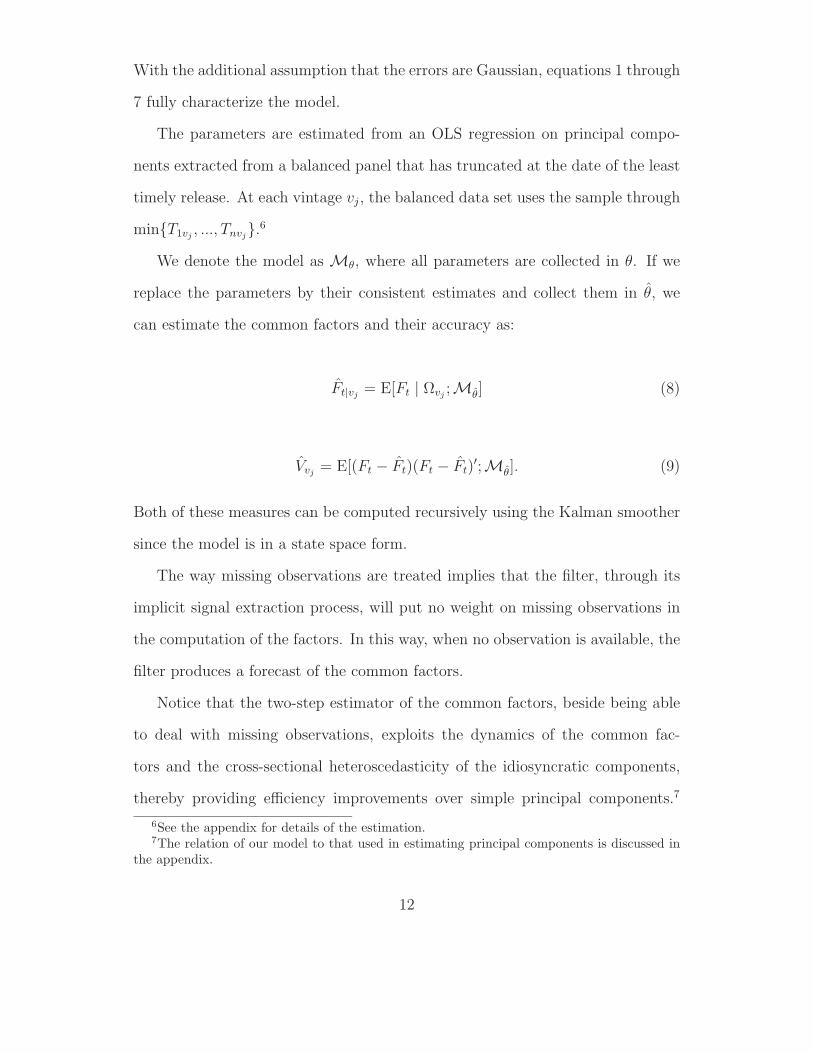
With the additional assumption that the errors are Gaussian, equations 1 through

7 fully characterize the model.

The parameters are estimated from an OLS regression on principal compo-

nents extracted from a balanced panel that has truncated at the date of the least

timely release. At each vintage vj, the balanced data set uses the sample through

minT1vj, ..., Tnvj

.6

We denote the model as Mθ, where all parameters are collected in θ. If we

replace the parameters by their consistent estimates and collect them in θ, we

can estimate the common factors and their accuracy as:

Ft|vj= E[Ft | Ωvj

;Mθ] (8)

Vvj= E[(Ft − Ft)(Ft − Ft)

′;Mθ]. (9)

Both of these measures can be computed recursively using the Kalman smoother

since the model is in a state space form.

The way missing observations are treated implies that the filter, through its

implicit signal extraction process, will put no weight on missing observations in

the computation of the factors. In this way, when no observation is available, the

filter produces a forecast of the common factors.

Notice that the two-step estimator of the common factors, beside being able

to deal with missing observations, exploits the dynamics of the common fac-

tors and the cross-sectional heteroscedasticity of the idiosyncratic components,

thereby providing efficiency improvements over simple principal components.7

6See the appendix for details of the estimation.7The relation of our model to that used in estimating principal components is discussed in

the appendix.

12

Doz, Giannone, and Reichlin (2006) have shown that the two-step estimator for

the common factors is consistent when the cross-section size, n, and the sample

size, T , are both large. Although the model does not allow for cross-sectional

and serial correlation of the idiosyncratic component, consistency is achieved un-

der more general assumptions. The key insight to understand this robustness

property of the estimator is the same as for simple principal components: due

to the law of large numbers, the idiosyncratic component becomes negligible as

the cross-sectional dimension increases. As a consequence, as far as it is confined

to the idiosyncratic part, the misspecification of the model does not compromise

consistency. For the same reason, the estimates of the common factors are likely

to be robust to the presence of data revisions provided the revision errors are

weakly cross-correlated.8

Given the estimates of the common factors, the nowcast of GDP can hence be

computed by estimating the coefficients α and β of equation (2) by OLS regression

of GDP, y3k, on the quarterly common factors, F3k|vj, using the sample for which

GDP growth is observed, k = 1, ..., ⌊Tyvj/3⌋ where Tyvj

is the last month for

which GDP is available for the vintage vj. The estimate for GDP is hence given

by:

y3k|vj= γ0 + γ′F3k|vj

.

The forecast h quarters ahead corresponds to the estimates made during the

months v = 3(k − h) − 2, 3(k − h) − 1, 3(k − h). For h = 0 we have the nowcast,

that is the estimate of GDP made during the current quarter.

The degree of precision of the estimate is computed as:

8See the appendix for details.

13

V y3k|vj= γ′V0|vj

γ + Var(e3k|vj),

where e3k|vj= y3k − y3k|vj

are the estimated residuals.

Notice that in our specification we do not include lagged GDP as predictor.

The reason is that, as we will show in the next Section, the common factors

are not only able to capture the bulk of dynamic interaction among monthly

indicators, but also the bulk of dynamics in GDP. This suggests that the sources

of GDP dynamics are common to those of the monthly series.

4 Empirics

As indicated in Section 2, the data set consists of about 200 macroeconomic indi-

cators for the US economy, including real variables (such as industrial production

and employment), financial variables, prices, wages, money and credit aggregates,

surveys from other sources, and other conjunctural indicators. Data are collected

in March 2005 with the sample starting in January 1982. They are transformed

to induce stationarity and to insure that the transformed variables correspond to

a quarterly quantity when observed at the end of the quarter. Details on data

transformations for individual series are reported in the appendix.

To examine the perfomance of the model, we perform two sets of exercises.

In the first, we provide an evaluation of the overall performance of the model.

We check how well the projection on the common factors tracks current-quarter

GDP, that is we look at the in-sample fit of the model. Moreover, we establish the

overall out-of-sample forecasting performance of the model using the information

available at the middle of each quarter.

14

In the second exercise, we study the effect of each release during the quarter on

the forecast accuracy; i.e., we analyze the evolution of the forecast in relation to

the flow of information throughout the quarter (we have 35 distinct data releases

in the quarter). We compute not only the model-based measure of accuracy but

also an out-of-sample measure that reflects model uncertainty.

For both exercises we aggregate the 35 releases in a stylized monthly calendar

of 15 releases. This is done because dates of publications are sometimes overlap-

ping. As will be detailed later, the calendar generally identifies a block of data

releases by both a publication date and an economic classification (all industrial

production series, labor and wage series, surveys and so on).

Because real-time vintages for all the series in the panel are not available,

we cannot perform a pure real-time evaluation. Therefore, the simulated out-of-

sample analysis is “pseudo” real time. The design of the exercise can be described

as follows. Because the timing and order of data releases vary only slightly from

month to month, we assume that the pattern of data availability is unchanged

throughout the evaluation sample. 9 More precisely, starting from January 1995

and until December 2004, each month the 15 real-time vintages are constructed by

replicating the pattern of data availability implied by the stylized calendar of the

15 data releases. Notice that, since we use data collected in March 2005, we are

not able to track data revisions. In this sense our vintages are “pseudo” real-time

vintages rather than fully real time vintages.10 We estimate the model recursively

using only information available at each point the nowcasts are computed.

We parameterize the model with two static factors and two common shocks:

9This assumption is not too unrealistic since the variation of the calendar over time are onlyminor.

10In the Appeniix, we compare the results on the performance of the nowcasts obtained using“pseudo” real-time vintages with those obtained by using real-time GDP vintages. It is shownthat using real-time GDP rather than revised GDP does not change the results qualitatively.

15

Figure 1: Realized GDP Growth versus Nowcast

Q1−85 Q1−90 Q1−95 Q1−00 Q1−05

−2

−1

0

1

2

3

4

5

6

7

8 GDPFM

q = 2, r = 2. This parametrization will be kept throughout the empirical exercise.

A robustness check using out-of-sample results for different choices of q and r is

provided in the appendix. As shown, our qualitative results are roubst with

respect to alternative values for these parameters.

4.1 Overall evaluation of the model

As shown in the previous section, the nowcast of current-quarter GDP growth is

obtained as a projection on the common factors. To verify that this procedure

provides a good in-sample fit, Figure 1 plots GDP growth against our nowcast.

As shown, our model tracks GDP growth quite well. In particular, it is effective in

capturing the two recessions of the sample – in the early 90s and at the beginning

of the new millennium.

Table 1 reports the autocorrelation function of the residuals of the projection.

The results indicate that only the autocorrelation at two quarters is marginally

16

significant and hence the residuals cannot be statistically distinguished from

white noise. This suggests that the few common factors extracted from our large

database of monthly indicators capture the bulk of GDP dynamics.

We now perform the out-of-sample evaluation of the model, comparing the

performance of our model with that of the the Survey of Professional Forecasts

(SPF). SPF forecasts are collected at the middle of each quarter. To make sure

that the results from our model are based on an information set comparable to

that available to the SPF forecasters, our model outcomes are based on data

available up to the end of the first week of the second month of each quarter, just

after the release of the Employment Report.

Forecast accuracy is measured by the Mean Square Forecast Error (MSFE).

The evaluation sample starts in the first quarter of 1995 and ends in the last

quarter of 2004. As a benchmark of non-predictability, we compute the forecasts

for a naive constant growth model.

Table 2 below reports the MSFE of the factor model and of the SPF relative

to the naive constant-growth model. A number below one indicates that the

forecasts are more accurate than those produced by the naive benchmark.

Results indicate that, beyond the first quarter, neither the SPF nor the factor

model are more accurate than the naive constant-growth model. Moreover, the

longer the forecast horizon, the worse is the relative forecast.11 Concerning the

current-quarter estimate (nowcast), some improvement over the naive model is

obtained by both the SPF and the factor model.

Figure 2 plots quarterly GDP growth against the constant growth model, the

factor model nowcast (FM), the SPF nowcast and the nowcast produced by the

11Giannone, Reichlin, and Sala (2004) find similar results in different sub-samples, indicatingthat our findings are robust.

17

Figure 2: Comparative Nowcast Results

Q1−95 Q3−97 Q1−00 Q3−02 Q1−05−2

−1

0

1

2

3

4

5

6

7

8

GBFMNaiveSPFGDP

Board of Governors of the Federal Reserve, the Greenbooks (GB), available to

the public only until the last quarter of 2000.

As is evident, our nowcast is effective in tracking GDP growth also when

estimated in real time. Moreover it compares well with both the Greenbook’s and

the SPF forecasts. The slow growth phase starting in 2001 is captured equally

well by both the SPF and our model. In the second half of the 90s, the Greenbook

and the SPF perform relatively poorly as they underestimate the surge in growth

associated with the boom in productivity, while the factor model has no bias over

this period.

We conclude that our estimates of current-quarter GDP growth have good

in-sample and out-of-sample performances. Hence, the model is well supported

by the data. It should be stressed that the model performs well at the horizon

where institutional forecasts, such as Greenbook’s and the SPF forecasts, have

been shown to outperform a simple constant growth model (Giannone, Reichlin,

18

and Sala 2004). At horizons longer than the current quarter, there is very little

forecastability for GDP (D’Agostino, Giannone, and Surico 2006). Clearly, the

current quarter is the horizon at which the timely exploitation of the early releases

matters most.

4.2 The marginal impacts of data releases on the accuracy

of the nowcast

Before conducting an analysis of the marginal impacts of individual data releases,

the calendar of data releases is reviewed in detail because the order of the releases

importantly affects their marginal impacts.

Stylized Calendar

The timing and structure of the data flows are described in Table 3. The 15

blocks into which the data releases have been are aggregated are listed in column

1, while the 35 individual releases are listed in column 2.12 Different blocks of

releases are published at different dates throughout a month (column 3) and may

refer to different dates (column 4). Typically, surveys have very short publishing

lags and often are forecasts for future months or quarters; while GDP, for example,

is released with a relatively long delay.13 Industrial production, prices, and other

variables are intermediate cases.

We start the month with the Chicago Report of the National Association of

Purchasing Management, which is released the first business day of the month.

We name this block “Survey 2” in the table. The next block comprises miscella-

12The source of each data release and the individual series in each release (and block) arereported in the appendix.

13The releases of the GDP and Income block for the first, second and third months of thequarter contain the GDP and Income data from the “advance,” “preliminary,” and “final”releases; respectively.

19

neous releases, such as construction spending and the advanced report on durable

goods manufacturers (“Mixed3”). “Mixed 3” is followed by “Money and Credit”

and so on.

Following the notation introduced in Section 2, v1 indexes the vintage after

the release of “Survey 2” and before the release of the second block “Mixed 3”.

Just after the inclusion of the “Financial” block, we have the last vintage of the

month, indexed by v15.

Because the data blocks defining the vintages are in the same order each

month, we use vj to index both the vintage and the time at which they are

released. We say that variables in the first block (“Survey 2”) are updated in

vintage v1 and are released at time v1.

The treatment of financial variables deserves a comment. Financial variables

and interest rates are the most timely of all the variables since they are avail-

able on a daily basis. Because the bulk of our data are monthly, we disregard

information from financial variables at frequencies lower than the month and let

these variables enter the model as monthly averages. We make the arbitrary as-

sumption that they become available only at the end of the month, which implies

that their impact on the estimation of the nowcast and its uncertainty will be

understated.

Because the stylized release calendar of 15 blocks roughly preserves the time

varying real-time release calendar and because the blocks include data series of

a similar economic content, our vintage data sets can be used sequentially to

examine the marginal impact of macroeconomic data releases on the nowcasts of

GDP growth.

20

The analysis

We now present two sets of results. First, we evaluate the in-sample evolution

of uncertainty over the quarter in relation to each release in the stylized calendar.

For each month of the current quarter v = 3k − 2, 3k − 1, 3k and for all data

releases within the month j = 1, ..., 15, we define uncertainty as:

V y3k|vj= E[(y3k|vj

− y3k)2],

where y3k|vjis the nowcast computed on the basis of the (incomplete) data at date

vj and y3k is realized current-quarter GDP growth. Because of the stationarity

assumption, our measure is invariant to the quarter in which we compute the

forecast. The measure depends only on the estimated parameters and on the

real-time data flow, which, accordingly to the stylized calendar, is the same in

every quarter. We evaluate it using parameters estimated over the entire sample.

Using the notation of Section 2, the nowcasts for quarter k are denoted by

y3k|vjfor the three months of the quarter, v = 3k−2, 3k−1, 3k and for each time

new macroeconomic data are released, j = 1, ..., J .

Second, we compute corresponding out-of-sample measures in order to check

for the robustness of the first set of results. Out-of-sample uncertainty, unlike the

corresponding in-sample measure, is influenced by model uncertainty and can be

taken as a further and tougher validation check of our model. In particular, we

look at the evolution of the MSFE for the nowcasts computed after each data

release within the quarter when GDP growth is projected on many monthly data

series. That is,

21

1

K1 −K0 + 1

K1∑

k=K0

(y3k|vj

− y3k

)2

v = 3k − 2, 3k − 1, 3k; j = 1, ..., 15

where the forecasts are computed recursively using only information available

at the time the nowcast is made. Unlike for the overall forecasting evaluation,

where the nowcast is computed at the end of the first week of the second month

of each quarter, here we track the evolution of the uncertainty of such nowcasts

throughout the quarter.

These two measures are derived from the analysis of the data releases in their

natural chronological order and thus correspond to the exercise in which the

forecaster updates her nowcasts after the release of each data block.

Results for the in-sample measure are reported in Figure 3, where uncertainty

is expressed relatively to the variance of GDP growth. The chart shows that intra-

month information matters. Data releases throughout the quarter convey new

information that is relevant because the uncertainty decreases uniformly through

the quarter.

The release that has the largest impact on the nowcast and its precision is the

“Mixed 2” block. “Mixed 2” is composed of two series from the “New Residential

Construction” release and nine series from the “Philadelphia Business Outlook

Survey”. By way of the Philadelphia survey, “Mixed 2” is the most timely release

since it is the first block containing data relating to the current month.

Results from the out-of-sample measure are described in Figure 4, which re-

ports the MSFE of the factor model relative to the constant-growth benchmark.

A value below one (dotted line), indicates that the nowcast from the factor model

outperforms that of the constant-growth model. The out-of-sample exercise con-

22

Figure 3: MSFE Across Data Blocks (In Sample)

0.47

0.49

0.51

0.53

0.55

0.57

0.59

0.61

0.63

0.65

Su

rveys

2

Mix

ed 3

Mon

ey &

Cre

dit

La

bo

r &

Wa

ges

Mix

ed 1

Ind

. P

rod

ucti

on

Mix

ed 2

PP

I

CP

I

GD

P &

In

com

e

Ho

usi

ng

Su

rveys

1

Init

ial

Cla

ims

Inte

rest

Ra

tes

Fin

an

cia

l

Su

rveys

2

Mix

ed 3

Mon

ey &

Cre

dit

La

bo

r &

Wa

ges

Mix

ed 1

Ind

. P

rod

ucti

on

Mix

ed 2

PP

I

CP

I

GD

P &

In

com

e

Ho

usi

ng

Su

rveys

1

Init

ial

Cla

ims

Inte

rest

Ra

tes

Fin

an

cia

l

Su

rveys

2

Mix

ed 3

Mon

ey &

Cre

dit

La

bo

r &

Wa

ges

Mix

ed 1

Ind

. P

rod

ucti

on

Mix

ed 2

PP

I

CP

I

GD

P &

In

com

e

Ho

usi

ng

Su

rveys

1

Init

ial

Cla

ims

Inte

rest

Ra

tes

Fin

an

cia

l

first month second month third month

firms that, as more information becomes available throughout the quarter, un-

certainty declines.

Notice that uncertainty corresponding to releases during the first month should

be seen as uncertainty around a forecast rather than nowcast uncertainty since,

in the first month, the only data release referring to the current quarter are the

Philadelphia Surveys (“Mixed 2”). During the first month, uncertainty around

the factor model forecasts is higher than that corresponding to the naive constant

growth model and the model is therefore not very reliable. This can also be seen

by the fact that, in the first month, the industrial production release (referring

to the previous month) increases uncertainty rather than reduces it.

From the second month onward, however, we confirm the feature of the in-

sample analysis where new information has a monotonic and negative effect on

uncertainty. In the first month, the distortion induced by “Industrial Production”

is corrected by “Mixed 2,” which, as in the in-sample evaluation, has a large

23

Figure 4: MSFE Across Data Blocks (Out of Sample)

0.6

0.7

0.8

0.9

1

1.1

1.2

Su

rveys

2

Mix

ed 3

Mon

ey &

Cre

dit

La

bo

r &

Wa

ges

Mix

ed 1

Ind

. P

rod

ucti

on

Mix

ed 2

PP

I

CP

I

GD

P &

In

com

e

Ho

usi

ng

Su

rveys

1

Init

ial

Cla

ims

Inte

rest

Ra

tes

Fin

an

cia

l

Su

rveys

2

Mix

ed 3

Mon

ey &

Cre

dit

La

bo

r &

Wa

ges

Mix

ed 1

Ind

. P

rod

ucti

on

Mix

ed 2

PP

I

CP

I

GD

P &

In

com

e

Ho

usi

ng

Su

rveys

1

Init

ial

Cla

ims

Inte

rest

Ra

tes

Fin

an

cia

l

Su

rveys

2

Mix

ed 3

Mon

ey &

Cre

dit

La

bo

r &

Wa

ges

Mix

ed 1

Ind

. P

rod

ucti

on

Mix

ed 2

PP

I

CP

I

GD

P &

In

com

e

Ho

usi

ng

Su

rveys

1

Init

ial

Cla

ims

Inte

rest

Ra

tes

Fin

an

cia

l

FM RW

first month second month third month

impact on the nowcast. In the second month; the “Labor and Wages” release,

which contains the first hard data relating to the current quarter, has a large

effect. In fact, only when the report on the employment situation of the second

month of the quarter (from the Bureau of Labor Statistics) is incorporated in

the estimates does the factor model become more accurate than the naive model.

Starting from that moment, results of the out-of-sample exercise confirmed what

was seen for the in-sample measure of forecast accuracy.14

In particular, these out-of-sample results confirm the earlier in-sample ones

showing the importance of “Mixed 2” and the fact that information contained

in industrial production does not have a role in reducing uncertainty because

it arrives relatively late in the quarter. Conditional on data released earlier,

industrial production does not induce a marginal reduction of uncertainty. This

highlights the importance of taking into account “timeliness” when measuring

14It is worth recalling that the nowcasts and the forecasts in Table 2 are computed just afterthe “Labor and Wages” release at the beginning of the second month.

24

the impact of data releases.

In summary, the results from the in-sample measure of accuracy are broadly

confirmed and they indicate that, in real time, the surveys are the most relevant

source of information for current quarter estimates of GDP. The out-of-sample

exercise attributes a larger role to “Labor and Wages” than what was seen in

the in-sample exercise, in particular at the beginning of the second month of the

quarter. Finally, both evaluation exercises have shown thatmore information

helps in reducing uncertainty.15

5 Summary and Conclusion

This paper has addressed a standard problem of real-time conjunctural analysis:

the forecast of current-quarter GDP growth in relation to the flow of data releases.

This problem has been analyzed with a non-standard tool that exploits the in-

formation in a large number of monthly variables, released in an asynchronous

way. The nowcasts are updated, each time new data are published, on the basis

of data sets with a “jagged edge” and which become progressively larger as time

evolves. In this way we offer a formal procedure to perform an exercise that, in

conjunctural analysis, is typically conducted on the basis of informal judgment.

The econometric model used in this analysis is a dynamic factor model where

15Other studies have evaluated the marginal impact of a block of variables by evaluating aforecast including or excluding the variables in question. Our exercise is different and moremeaningful to handle the real time aspect of data flow, in particular when data are nearlycollinear as it is the case for macroeconomics series. For example, in the extreme case in whichtwo blocks of variables are perfectly collinear, using each block separately would produce thesame forecasts indicating that the two blocks are equally important. In real time, however,the marginal contribution of a particular block depends on the order of data arrival. In theexample above of perfectly collinear blocks of variables, only the block that is released first hasinformation content since, by the time the later release is published, its informational contentis already incorporated in the forecast.

25

the factors are estimated in two steps: first computing principal components and

then using the Kalman smoother. The consistency properties of this methodology

have been shown by Doz, Giannone, and Reichlin (2006).

This paper provides an out-of-sample empirical evaluation that shows the

model fares well relative to several benchmarks. We use that method to evalu-

ate quantitatively how information from various sources affects our assessment

of current economic conditions by estimating the effect of each release on the

accuracy of the nowcast.

Empirical results show that within-quarter data flows matter in the sense that

the precision of the nowcast generally increases monotonically as new information

becomes available during the current quarter. This result lends support to the

idea that exploiting rich data sets is very relevant for real-time data analysis. We

also show that the timing of releases is a key determinant of the size of the release’s

marginal predictive power. In particular, the Philadelphia Federal Reserve Bank

surveys, which are released early in the month, have a large positive effect on

forecasting accuracy. Our out-of-sample exercise shows that this is also true for

the report on the employment situation.

26

References

Altissimo, F., A. Bassanetti, R. Cristadoro, M. Forni, M. Hallin,

M. Lippi, and L. Reichlin (2001): “EuroCOIN: A Real Time Coincident

Indicator of the Euro Area Business Cycle,” CEPR Discussion Papers 3108.

Baffigi, A., R. Golinelli, and G. Parigi (2004): “Bridge Models to Forecast

the Euro Area GDP,” International Journal of Forecasting, 20(3), 447–460.

Bai, J. (2003): “Inferential Theory for Factor Models of Large Dimensions,”

Econometrica, 71(1), 135–171.

Bai, J., and S. Ng (2002): “Determining the Number of Factors in Approximate

Factor Models,” Econometrica, 70(1), 191–221.

Boivin, J., and S. Ng (2005): “Understanding and Comparing Factor-Based

Forecasts,” International Journal of Central Banking, 3, 117–151.

Chow, G. C., and A.-l. Lin (1971): “Best Linear Unbiased Interpolation,

Distribution, and Extrapolation of Time Series by Related Series,” The Review

of Economics and Statistics, 53(4), 372–75.

Croushore, D., and T. Stark (2001): “A Real-Time Data Set for Macroe-

conomists,” Journal of Econometrics, 105(1), 111–130.

D’Agostino, A., and D. Giannone (2006): “Comparing Alternative Predic-

tors Based on Large-Panel Dynamic Factor Models,” Working Paper Series

680, European Central Bank.

27

D’Agostino, A., D. Giannone, and P. Surico (2006): “(Un)Predictability

and Macroeconomic Stability,” Working Paper Series 605, European Central

Bank.

Doz, C., D. Giannone, and L. Reichlin (2006): “A Two-Step Estimator

for Large Approximate Dynamic Factor Models Based on Kalman Filtering,”

Unpublished manuscript, Universite Libre de Bruxelles.

Evans, M. D. (2005): “Where Are We Now? Real-Time Estimates of the

Macro Economy,” NBER Working Paper 11064, Internationa Journal of Cen-

tral Banking, forthcoming.

FED, C. (2001): “CFNAI Background Release,” Discussion paper, http://

www.chicagofed.org/economicresearchanddata/national/pdffiles/CFNAI

bga.pdf.

Forni, M., D. Giannone, M. Lippi, and L. Reichlin (2005): “Opening the

Black Box: Structural Factor Models with large Cross-Cections,” Manuscript,

Universite Libre de Bruxelles.

Forni, M., M. Hallin, M. Lippi, and L. Reichlin (2005): “The Generalized

Dynamic Factor Model: One-Sided Estimation and Forecasting,” Journal of

the American Statistical Association, 100(471), 830–840.

Giannone, D., L. Reichlin, and L. Sala (2004): “Monetary Policy in Real

Time,” in NBER Macroeconomics Annual, ed. by M. Gertler, and K. Rogoff,

pp. 161–200. MIT Press.

28

Kitchen, J., and R. M. Monaco (2003): “Real-Time Forecasting in Prac-

tice: The U.S. Treasury Staff’s Real-Time GDP Forecast System.,” Business

Economics, pp. 10–19.

Koenig, E. F., S. Dolmas, and J. Piger (2003): “The Use and Abuse

of Real-Time Data in Economic Forecasting,” The Review of Economics and

Statistics, 85(3), 618–628.

Marcellino, M., J. H. Stock, and M. W. Watson (2003): “Macroeco-

nomic Forecasting in the Euro Area: Country Specific versus Area-Wide Infor-

mation,” European Economic Review, 47(1), 1–18.

Orphanides, A. (2002): “Monetary-Policy Rules and the Great Inflation,”

American Economic Review, 92(2), 115–120.

Runstler, G., and F. Sedillot (2003): “Short-Term Estimates Of Euro Area

Real Gdp By Means Of Monthly Data,” Working Paper Series 276, European

Central Bank.

Stock, J. H., and M. W. Watson (2002a): “Forecasting Using Principal

Components from a Large Number of Predictors,” Journal of the American

Statistical Association, 97(460), 147–162.

(2002b): “Macroeconomic Forecasting Using Diffusion Indexes,” Journal

of Business and Economics Statistics, 20(2), 147–162.

29

Table 1: Tracking GDP Growth with the Factor Model: ACF of the Residuals

lag (m) 1 2 3 4acf -0.01 0.22 0.03 0.03

p-value 0.93 0.05 0.81 0.81

Autocorrelation function of the residual of the projection of GDP growth on the commonfactors. P-values refer to the Ljung-Box Q-statistics for the null of no serial correlation up toorder m.

30

Table 2: Nowcasts and Forecasts of GDP: Out-of-Sample Evaluation.

Horizon 0 1 2 3 4FM 0.91 1.05 1.10 1.25 1.18SPF 0.94 1.15 1.29 1.29 1.36

Mean Squared Forecast Errors of GDP growth for the Factor Model (FM) and Survey ofProfessional Forecasters (SPF) relative to a naive constant growth model for GDP. Evaluationsample: 1995q1-2004q4.

31

Table 3: Calendar of Data Releases within the Month

Block Name (1) Release (2) Timing Publishing Frequency(approx.) (3) Lag (4) of data (5)

Surveys 2 PMGR-Manufacturing 1st business day of month one month MonthlyMixed 3 Commercial Paper outstanding 1st bus. day of month one month MonthlyMixed 3 Construction Put in Place 1st bus. day (or slightly before) two months MonthlyMixed 3 Advance Report on Durable Goods Manufacturers Shipments, Inventories and Orders 1st. bus. day (or slightly before) one month MonthlyMixed 3 Full Report on Durable Goods Manufacturers Shipments, Inventories and Orders 5 days after Advance Durables two months MonthlyMoney & Credit Consumer Delinq. Bulletin Quarterly (series is monthly) two quarters MonthlyMoney & Credit Aggregate Reserves of Depository Institutions and the Monetary Base 1st Thurs. of month one month MonthlyMoney & Credit Money Stock Measures 2nd Thurs. of month one month MonthlyMoney & Credit Assets and Liabilities of Commercial Banks in the United States 1st Fri. of month two months MonthlyLabor & Wages Employment Situation 1st Fri. of month one month MonthlyMixed 1 Consumer Credit 5th business day of month two months MonthlyMixed 1 Advance Monthly Sales For Retail and Food Services 11-15th of month one month MonthlyMixed 1 Monthly Treasury Statement of Receipts and Outlays of the U.S. Government Middle of month one month MonthlyMixed 1 FT900 U.S. International Trade in Goods and Services: Exhibit 5 2nd full week of month two months MonthlyInd. Production Industrial Production and Capacity Utilization 15th to 17th of month one month MonthlyMixed 2 New Residential Construction 16th to the 20th of month one month MonthlyMixed 2 Business Outlook Survey: Federal Reserve Bank of Philadelphia 3rd Thursday of month current month MonthlyPPI Producer Prices Middle of month one month MonthlyCPI Consumer Prices Middle of month one month MonthlyGDP & Income GDP - detail: inventories and sales Day after GDP - release two months MonthlyGDP & Income GDP - release: GDP and GDP deflator Last week of month one quarter QuarterlyGDP & Income Personal Income and Outlays Day after GDP - release one month MonthlyHousing Manufactured Homes Survey 3rd to last bus. day of month one month MonthlyHousing New Residential Sales Last week of month one month MonthlySurveys 1 Chicago Fed Midwest Manufacturing Index Last week of month one month MonthlySurveys 1 Consumer Confidence Index Last Tues. of month current month MonthlySurveys 1 Michigan Survey of Consumers Last Fri. of the month current month MonthlyInitial Claims Claims, Unemployment Insurance Weekly Claims Report Last Thurs. of month: Monthly ave. current month WeeklyInterest Rates Freddie Mac Primary Mortgage Survey Last Wed. of month: Monthly ave. current month WeeklyInterest Rates Selected Interest Rates Last day of month: Monthly ave. current month DailyFinancial Foreign Exchange Rates Last day of month: Monthly ave. current month DailyFinancial London Gold PM Fix Last day of month: Monthly ave. current month DailyFinancial New York Stock Exchange Last day of month: Monthly ave. current month DailyFinancial S&P Indices Last day of month: Monthly ave. current month DailyFinancial Wilshire Index Last day of month: Monthly ave. current month Daily

Data releases are indicated in rows. Column 1 reports the block in which the released data are included. Column 2 indicates the releases.Column 3 indicates the official dates of the publication. Column 4 report the period up to which the data are reported. The native frequencyof the data is reported is Column 5. Typically, surveys have very short publishing lags and often are forecasts for future months or quarters,while GDP, for example, is released with a relatively long delay.a

32