Nowcasting the Czech Trade Balance - ETSG · Nowcasting the Czech Trade Balance Oxana Babecká...

Nowcasting the Czech Trade Balance

Oxana Babecká Kucharčuková and Jan Brůha

Abstract

In this paper we are interested in nowcasting and short-run forecasting of the main external

trade variables. We consider four empirical methods: principal component regression, elastic

net regression, the dynamic factor model and partial least squares. We discuss the adaptation

of those methods to asynchronous data releases and to the mixed-frequency set-up. We

contrast them with a set of univariate benchmarks. We find that for variables in value terms

(both nominal and real), elastic net regression typically yields the most accurate predictions,

followed by the dynamic factor model and then by principal components. For export and

import prices, univariate techniques seem to have the higher precision for backcasting and

nowcasting, but for short-run forecasting the more sophisticated methods tend to produce

more accurate forecasts. Here again, elastic net regression dominates the other methods.

JEL Codes: C53; C55; F17.

Keywords: Dynamic factor models, elastic net regression, mixed-frequency data,

nowcasting, principal component analysis, state space models, trade

balance.

Oxana Babecká Kucharčuková, External Economic Relations Division, Czech National Bank

(email: [email protected]);

Jan Brůha, Economic Research Department, Czech National Bank (e-mail: [email protected]).

The authors would like to thank Gabriel Perez Quiros, Jan Babecký, Tomáš Holub, Jiří Polanský and Luboš

Růžička for their valuable comments. This work was supported by Czech National Bank Research Project

No. B1/14. The support is gratefully acknowledged.

The views expressed in this paper are those of the authors and not necessarily those of the Czech National Bank.

2 Oxana Babecká Kucharčuková and Jan Brůha

Non-Technical Summary In recent years, nowcast models have become a popular econometric tool for current-quarter

nowcasting and short-term forecasting of GDP. A nowcast model is an empirical model based

on a broad range of time series with different lengths and publication frequencies and lags. By

construction, the model is able to account for the most recent information, which is not

always straightforward due to broad dispersion of publication lags across series. For instance,

the lag can be zero or slightly positive in the case of leading indicators, but for Czech national

accounts subcomponents it exceeds two months.

In contrast to previous studies focused on GDP, this paper presents nowcast models for

external trade, Czech external trade in our case. To the best of our knowledge, no nowcast

model for trade has been described in the literature so far. Exports and imports are exposed to

foreign shocks, which increases the importance of foreign variables for nowcast models.

Furthermore, in contrast to GDP growth, which is mainly meaningful in real terms, for trade

both real and nominal developments (BoP statistics) are important.

Once the model is set up, regular updates can be produced as new data become available. Fast

incorporation of the latest information is one of the reasons why nowcast modelling is of great

interest not only to researchers, but also to central bankers. Indeed, the model described in this

paper is also intended to be used for regular forecasting at the CNB as an alternative or

complement to existing econometric models as well as to the core CNB model.

Nowcasts and short-term forecasts are prepared for nine variables. Four of them have

quarterly frequency: exports and imports from the national accounts statistics at both constant

and current prices. Monthly nowcasts are produced for nominal trade (exports and imports

separately) and the relevant price indexes. In addition, given the high importance of the

foreign PPI for the Czech economy, the result for the foreign effective PPI is also shown here.

All variables are transformed into growth rates relative to the corresponding period of the

previous year. As for explanatory variables, five groups of economic and financial indicators

are used for this purpose. Roughly half of them describe domestic developments. The

remaining half describe the foreign sector – mainly the euro area, but also Germany and the

United States. The sample span starts in January 2006 or 2006q1 and ends in September 2016,

or 2016q2 in the case of quarterly data.

The quality of the nowcasts is evaluated using a pseudo-real time framework, which mimics

the actual publication lag structure and is compared across four empirical models: principal

component regression, elastic net regression, the dynamic factor model and partial least

squares. For exports and imports in both nominal and real terms, as well as for trade price

indexes, the winner is elastic net regression. The forecasting performance of the elastic net is

better even than that of the dynamic factor model, which is widely believed to produce the

most accurate nowcasts, at least for GDP. The other methods could be used as alternative

checks. In addition, the dynamic factor model could be used to create alternative scenarios

using conditional forecasts.

Nowcasting the Czech Trade Balance 3

1. Introduction

Interest in nowcasting has increased dramatically over the last decade. This forecasting technique

is now widely applied by many central banks and research institutions across the globe.

Nowcasting usually refers to forecasting of the recent past and present values of an economic

indicator not yet available due to low frequency and publication delay, and to short-term

forecasting of that indicator. Missing and future values are projected on a set of relevant variables

having the same or higher frequency but shorter or zero time lags. Because new data releases

appear in an asynchronised manner (creating a ragged edge problem), nowcast models are

designed to be able to produce updated forecasts immediately as new information becomes

available. This type of forecast is often prepared as a judgment-free forecast that tries to reap data

from a large set of indicators that may contain useful, but scattered, pieces of information.

Although data-driven estimation can be considered a model weakness, fast incorporation of the

latest information, good forecasting performance at shorter horizons and the use of rich dataset are

certainly big advantages of this technique.

At the central bank, nowcast models are useful as a complementary tool to other forecasting

techniques such as large structural models (i.e. DSGE models). Their ability to incorporate newly

released data immediately into the forecast is beneficial for timely assessment of changes in

economic developments. Furthermore, current-period forecasts from nowcast models can serve as

inputs to DSGE models, where a more precise forecast at the beginning of the forecasting horizon

by construction increases the accuracy of forecast at its end (del Negro and Schorfheide, 2013).

Although the main CNB forecasting tool is a DSGE model called g3 (Andrle et al., 2009),

nowcasts and near-term forecasts are discussed in depth at the beginning of each prediction round

(Brůha et al., 2013). Camacho, Perez-Quiros and Poncela (2013) give an overview of empirical

techniques that can be used for nowcasting and short-run forecasting.

GDP growth is the most frequently nowcasted indicator. This key measure of economic activity is

published with a considerable delay, and the Czech Republic is no exception. The time lag is

particularly striking in the case of GDP subcomponents – investment, consumption and external

trade, where new data become available with a lag of more than two months. In addition, frequent

revisions of national accounts introduce higher uncertainty about the precision of the latest data

and make the forecasting exercise more challenging.1 Nowadays, GDP growth nowcasts are

produced for all the most important economies, for example the USA, the euro area, Germany and

even China.

For the Czech Republic, an aggregated GDP growth nowcast is prepared at the CNB and regularly

used as an alternative forecast during the quarterly forecasting exercise. Several models have been

developed for this purpose. Arnoštová et al. (2011) build nowcast models using monthly

indicators. The authors compare results based on a simple autoregression model and bridge

equations with those obtained from principal components and dynamic factor models. They find

that the principal components model has the best predictive power up to three quarters ahead.

1 As an illustration see, for instance, Appendix A in Brůha et al. (2013).


Beyond this horizon, the most precise forecast is the near-term forecast of the CNB model.

Rusnák (2013) evaluates the forecasting performance of dynamic factor models using vintage data

and accounting for publication lag. The author also stresses the importance of foreign variables

for Czech GDP nowcasting. His results suggest that the nowcasting performance of the medium-

scale dynamic factor model is comparable with the CNB’s judgmental nowcasts. Finally, Franta et

al. (2014) extend the two above-mentioned analyses and focus on several types of mixed-

frequency data models: mixed-frequency VAR, a mixed-data sampling model and a dynamic

factor model. The authors find that in the short term the dynamic factor model is comparable with

the CNB’s forecasts. At longer horizons, the mixed-frequency VAR and BVAR models slightly

outperform the CNB’s forecasts.

In contrast to previous studies, the purpose of the present analysis is to construct and estimate a

set of nowcast models for the Czech trade balance. To the best of our knowledge, there is no

nowcast model focused on Czech external trade and there is no description of a nowcast trade

model in the literature. Although net exports are a part of GDP, a nowcast model designed for

GDP is not directly applicable to external trade for a number of reasons. First, external shocks are

more important in the case of trade than in the case of GDP on aggregate. The use of a “universal

model” with hundreds of time series for both GDP and trade may not be an appropriate solution.

As previous research shows, a nowcast model based on a very large dataset containing hundreds

of economic and financial indicators does not produce a better forecast than a model with fewer,

but carefully selected, inputs (Boivin and Ng, 2006). Second, recent research shows that the

elasticity between trade growth and GDP growth has changed since the crisis (ECB, 2016). As the

relation between trade and GDP is time-varying, the good fit of GDP models may not hold for

trade over the whole sample period. Third, GDP growth models are by construction focused on

forecasting of real variables. In the case of external trade, forecasts at both current and constant

prices are important. Constant prices allow the results to be compared with the core DSGE model

and used as DSGE inputs. Nominal prices give us an idea about the evolution of an important part

of the balance of payments (BoP). However, national accounts, cross-border and BoP statistics are

not fully identical. BoP statistics are available at current prices only and released and revised

independently of the national accounts statistics. Thus, our intention is to construct a nowcast

model of Czech exports and imports in both nominal and real terms. The main reason for doing so

is the planned regular use of this model for making alternative estimates during the quarterly

forecasting exercise at the CNB. The results will be compared with the CNB’s econometric

models – forecasts of trade at constant prices and price indexes. Furthermore, a direct nowcast at

current prices allows for straightforward comparison with the trade balance forecast based on BoP

statistics, which is available at current prices only. In addition to unconditional forecasting, one of

our estimation techniques will allow for conditional forecasting and, by consequence, scenario

analysis based, for example, on different assumptions about foreign GDP or foreign PPI growth,

which could also be used at the CNB.

The structure of the paper is the following. The next two sections describe the data we use.

Section 4 explains the methodology applied for nowcasting and short-term forecasting of the

Czech trade balance and shows the results for the Czech economy. Section 5 compares the

forecasting performance of the methods, and the final section 6 concludes. Appendices contain

additional materials.


2. Data

In this paper, we present nowcasts and short-term forecasts of the main external trade variables:

exports and imports and their prices. All the variables are transformed into yearly growth rates.2

We are primarily interested in nominal and real exports and imports published as part of the

national accounts statistics. These data are released at quarterly frequency and can be used

directly as near-term forecasts for the main g3 model. In addition, we consider monthly nominal

exports and imports published by the Czech Statistical Office for nowcasting of the trade balance

at monthly frequency. We are also interested in import and export prices at monthly frequency.

Furthermore, we apply the chosen methods to the effective foreign producer price index (PPI),

also taken at a yearly growth rate. This variable is important for the CNB’s macroeconomic

forecast for at least two reasons. First, the foreign PPI is a proxy for foreign inflation pressures on

the Czech economy in the CNB’s main forecasting model. Second, the relative price of Czech

exports in the g3 model is the ratio of the foreign PPI to Czech export prices.

To sum up, we are interested in nowcasts of nine variables. Four of them are of quarterly

frequency, namely the nominal and real growth rates of exports and imports from the national

accounts. The remaining five are of monthly frequency: the growth rates of nominal exports and

imports, their price indexes and the foreign PPI.

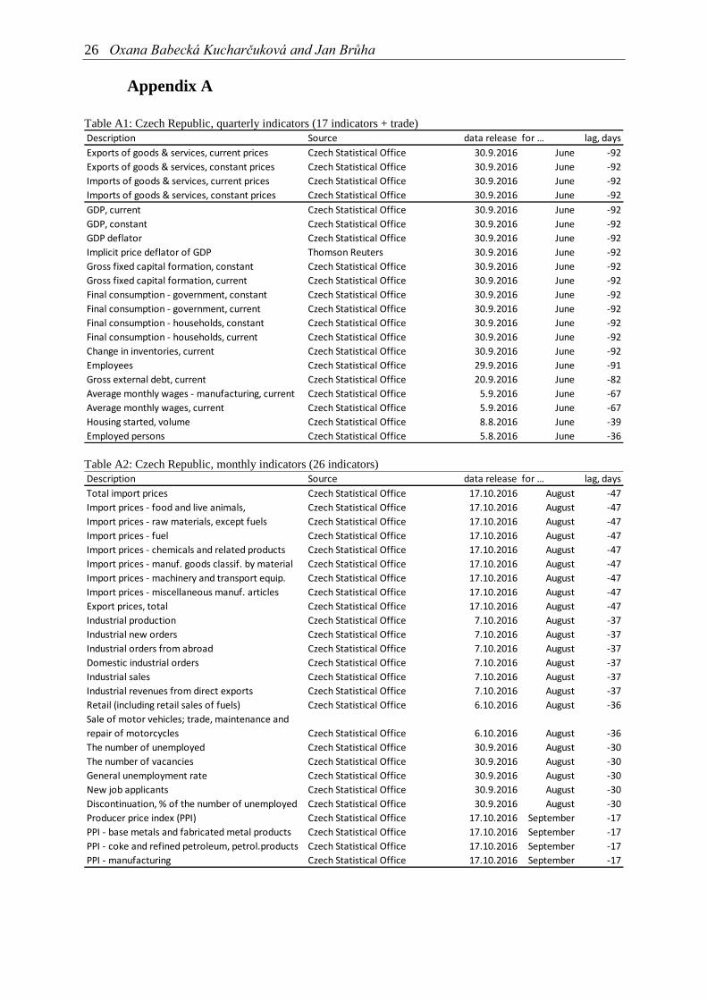
As for predictors for the nowcast and short-term forecast, we collected a large dataset of variables

that can be used for predicting the variables of interest. These variables are listed in Appendix A

along with their sources and publication lags.

Our dataset runs from January 2006 to September 2016 (monthly time series) and from 2006Q1 to

2016Q2 (quarterly series). All data are in yearly growth rates, which are the percentage change

relative to the same period (month or quarter) of the previous year. We do not work with data

prior to 2005 so as to avoid the structural break in the Czech trade data time series related to EU

entry in May 2004.

3. Descriptive Statistics

The components of Czech trade have been steadily increasing in both nominal and real terms

since the start of the economic transition. The entry of the Czech Republic to the European Union

in May 2004 caused an upward shift in both the level and the trend growth rate of exports and

imports. The only significant drop in the volumes and values of exports and imports occurred

during the 2008/2009 recession, but this was quickly reversed and by 2011 the figures were back

at their pre-crisis levels.

2 While for monthly data these are, by construction, moving averages of the monthly growth rates,

transformation into one-period change introduces additional noise and extracting seasonality may reduce the

precision of the estimates. Furthermore, yearly growth rates make the results more comparable with those of

other CNB models during the regular forecasting exercise. As we intend to use the model at the CNB for regular

forecasting, we selected this method of transformation. Last but not least, we run the nowcast model on one-

period transformed data. The results obtained are broadly comparable with the yearly growth rates and lead to

the same conclusion as in the case of nowcasts based on yearly growth rates.


The evolution of real exports and imports is displayed in the upper subfigure of Figure 3.1, where

both EU entry and the 2008–2009 recession are clearly visible. The lower subfigure shows that

the openness of the Czech economy has been increasing as well: the ratios of both nominal

exports and nominal imports to nominal GDP have increased from about 45% in the pre-EU entry

period to about 80% now. This means that the trend growth rates of the two trade balance

components have been significantly higher (by about 4% annually) than the trend growth rate of

GDP. EU entry almost immediately increased the openness share by about 10 p.p.

Figure 3.1: Czech exports and imports through time

It is not only the level of exports and imports that is important for the Czech economy. Both series

are also strongly cyclical. This is illustrated in Figure 3.2. The upper subfigure shows the annual

growth rates of exports, imports and GDP (which is multiplied by a factor of 4). The

comovements in the growth rates are clearly visible. The comovements are even greater for the

cyclical components shown in the lower subfigure: here, the cyclical components were isolated

using the univariate Christiano-Fitzgerald filter and correspond to frequencies of 6 to 32 quarters.


Figure 3.2: Cyclical characteristics of Czech exports and imports

Apparently, real exports and imports lead real GDP by one quarter. This can be seen from the

following Figure 3.3, which displays the sample correlation of the quarterly growth rates and the

cyclical components of these variables for various lags and leads (these are in quarters).


Figure 3.3: Correlations between real exports and imports and GDP

The correlation is especially strong for the cyclical components and peaks at the first quarter lead,

i.e., the real export and import cycles lead the GDP cycle by one quarter. The correlations

between quarterly growth rates are rather lower, but the pattern of a one-quarter lag still holds.

Looking at monthly data, the values of Czech exports and imports are significantly correlated with

both Czech and German industrial production in manufacturing. This is illustrated in Figure 3.4,

which shows both the yearly growth rates and the cyclical components of these variables. The

correlation between Czech exports and imports and both industrial productions peaks at the zero

lag and attains a value of 0.8 for growth rates and 0.95 for the cyclical components in the case of

Czech industrial production. The correlation with German industrial production is rather lower,

but still impressive: 0.7 for growth rates and 0.85 for the cyclical components. These four series

comove contemporaneously. Czech exports and imports are also correlated with various measures

of business confidence. To sum up, exports and imports are strongly cyclical variables in the case

of the Czech Republic.


Figure 3.4: Exports, imports and industrial production

Finally, Figure 3.5 displays the yearly growth rates of export and import prices and the Czech,

German and foreign effective PPI.3 The figure also shows the correlations of export and import

prices with the three PPI series. Czech export price growth is weakly correlated with the Czech

PPI. Export price growth leads domestic PPI growth by three or four months, i.e. knowing today’s

export prices can help in predicting the Czech PPI. However, the correlation is not strong. The

series is almost uncorrelated with the foreign and German PPI. The low correlation is due to the

2009 episode of a sudden and temporary depreciation of the Czech koruna. On the other hand,

import price growth is well aligned with both German and foreign effective PPI growth (both

expressed in Czech currency). The effect of the exchange rate floor on the Czech koruna

introduced in November 2013 is clearly visible in the import price series.

3 The effective PPI is a weighted PPI of 14 euro area members, which enter the index according to the

importance of Czech exports to those countries. The euro area is the Czech Republic’s main trade partner.

Roughly half of total Czech exports to the euro area go to Germany. The export share to Slovakia is 14% and

those to Austria, France and Italy are between 6% and 8% of total Czech exports to the euro area (nominal

prices).


Figure 3.5: Export and import prices and their correlation with the PPI

4 Methods and Results

The nowcast and short-term forecast methods can be characterised as an attempt to distil the

information content from indicators, in particular from those which are available sooner than the

data of interest. The methods selected for our analysis are adapted to mixed-frequency

frameworks and to asynchronous data releases. Leaving aside the potential complexities arising

from mixed frequency, all the methods considered here can be classed as data shrinkage

procedures. The forecast of the variable yt+k|t at horizon t+k given the data available at time t 𝐷𝑡

can be written as follows:

𝑦𝑡+𝑘|𝑡 = Λ𝐾𝐷𝑡. (1)

With an infinite sample, such a prediction can be estimated just by OLS. With a large number of

possibly highly correlated predictors in 𝐷𝑡, the OLS approach would obviously yield a very poor

prediction due to the unreliability of the estimation of matrix Λ𝑘. Nowcast estimation methods

differ in the way the projection matrix k is generated so as to avoid the curse of dimensionality

caused by a large number of possible predictors in 𝐷𝑡. Carrasco and Rossi (2016) provide a nice

discussion of a unifying framework behind the estimation of predictive equations when dataset Dt

is large.


The comparison of forecast methods is based on a pseudo-real time forecast,4 where we respect

the lag structure of the published data. We use two main statistics: the root mean square error

(RMSE) and the mean absolute error (MAE). For most cases, the two statistics give the same

ranking of relative forecast performance. Only in a very few cases where the two methods show

similar forecast performance do the rankings of the two statistics differ. In such cases, however,

the differences between the two methods are immaterial. Readers interested in whether there is a

systematic correlation between the forecast errors for our variables of interest are referred to

Appendix C.

We compare all our models against six univariate benchmark models: (i) usual random-walk

predictions, (ii) predictions based on the unconditional past mean of the series, (iii) predictions

based on various forms of exponential smoothing (see Hyndman et al., 2008, for an overview),

(iv) autoregressive (AR) models of various lags, (v) Bayesian AR models that shrink the

coefficients towards zero, and (vi) time-varying AR models.

Turning to the lag structure, for the monthly time series of nominal exports and imports, the best

univariate prediction models were obtained from large AR models with four to six lags. The

differences between the lags at these horizons are small and insignificant. Also, Bayesian AR

models and AR models with time-varying parameters provide only a marginal improvement

compared to plain-vanilla OLS estimation.5 Again, the differences between these two more

sophisticated variants and the standard AR models – for a given lag – are both statistically and

economically insignificant.

For the monthly series of the price indexes, the best univariate models are either low-lag AR

models or the exponential smoothing model. Again, the differences between the usual AR models

and their more sophisticated counterparts are not significant. For these series, the unconditional

mean forecast (i.e. the forecast that sets the forecasted values at their past unconditional means)

tends to be as good as these forecasts for longer forecast horizons. Detailed results for the

univariate models can be found in Appendix B.

4.1 Principal Component Regressions

This method is based on the estimation of principal components (PC), i.e. a low-dimensional

object that spans the data. Instead of regressing the forecasted variables on the set 𝐷𝑡 as in (1), the

PC prediction starts with estimation of a low number of mutually orthogonal series – principal

components – that span sufficiently well the space of data available 𝐷𝑡. Since the dimension of the

principal components is low and because they are orthogonal, regression of future values on them

is much more efficient than regression on the original variables.

4 Given that the historical time series of GDP and its subcomponents were recently subject to special major

revision, estimation of model performance and forecast evaluation on true vintages will, in our opinion, be less

reliable for the planned future regular practical application of the model compared to the pseudo-real time

forecast applied here. 5 In fact, although we allowed a significant degree of time variation of the AR coefficients, the estimated time-

varying AR coefficients drift very little.


The principal components can be easily derived from the eigenvalue decomposition of the

covariance matrix (Bai and Ng, 2002). To impute any missing data,6 the EM algorithm is used;

see Stock and Watson (2002) or Foroni and Marcellino (2013).

As the highest frequency of our data is monthly, the dataset used to span the principal components

operates at monthly frequency and hence the principal components also have monthly frequency.

Given the estimate of the principal components, the forecast of variables operating at monthly

frequency is straightforward:

𝑦𝑡+𝑘|𝑡𝑚 = Λ𝑘𝑓𝑡 + 𝜚𝑦𝑙(𝑡), (2)

where 𝑓𝑡 is the vector of estimated principal components at time t. As it is common, we include

the last available value of the forecasted variable yl(t) as an additional predictor.7 The symbol 𝑙(𝑡)

denotes the last observation of the forecasted variable available at time t, which for our

application is typically 𝑡 − 1. Given the estimated principal components, the estimation of the

matrix Λ𝑘 and of the autoregressive term 𝜚 is quite straightforward and can be done using OLS.

The forecast for the quarterly variables is generated as follows:

𝑦𝑡𝑄+𝑘|𝑡𝑄𝑄

= Λ𝑘𝑐(𝐿)𝑓𝑡 + 𝜚𝑦𝑙(𝑡𝑄), (3)

where 𝑐(𝐿) is the polynomial in the lag operator L that aggregates the monthly series to quarterly

frequency.

We estimate the predictive equations for a number of principal components ranging from one to

six. The number of components was based on the forecasting accuracy. It turns out that the best

forecasting performance for all nine time series considered is achieved with four principal

components.

We also experimented with time variation in Equations (2) and (3) by making the projection

matrices Λ𝑘 time varying. We did this in a relatively unsophisticated but robust way by means of

weighted least squares where, in estimating Λ𝑘 at time t, more distant observations receive lower

weights according to exponential decay. We find that the use of such time variation did not

improve the forecasting properties of the model and the cross-validated choice of forgetting factor

was very close to 1, meaning no preference for time variation. Therefore, we do not report these

results below.

The resulting recursive forecasts are displayed in Figure 4.1. For export and imports, the model

seems to capture the turning points around the Great Recession, although it was not able to fully

foresee the significant trade increase that occurred in 2014.

6 For our data, this occurs typically at the end of the sample, but more general patterns of missing data can be

considered. 7 To our surprise, this autoregressive term is important for backcasting and nowcasting only. For near-term

forecasting it is not necessary and its inclusion even makes the forecast slightly less accurate.


We use our own Matlab codes to estimate the principal components, to impute missing values by

the EM algorithm and to estimate predictive equations (2) and (3) or their time-varying

counterparts.

Figure 4.1: Recursive predictions using principal components

4.2 Elastic Net Regression

While the principal component approach attempts to solve the curse of dimensionality by

constructing a low number of mutually orthogonal principal components, there are regularisation

techniques that control the number and/or the magnitude of the regression coefficients of (1)

directly.

Elastic net regression (Zou and Trevor, 2005) is a linear regularised regression method that

combines both so-called L1 and L2 penalties; hence it covers as a special case both Lasso (L1

penalty only) and ridge (L2 penalty only) regressions. This method estimates the regression

coefficients of a variable 𝑌 on 𝑋 as a solution to the following problem:

𝛽 = 𝑎𝑟𝑔𝑚𝑖𝑛{∑ (𝑌𝑖 − ∑ 𝑋𝑖𝑙𝛽𝑙𝑙 )2𝑖 − 𝜆1∑ |𝛽𝑙|𝑙 − 𝜆2∑ 𝛽𝑙2

𝑙 }, (4)

where 𝜆1 and 𝜆2 are two positive constants. We use the elastic net to estimate the reduced-form

forecasting relationship between the variables of interest 𝑦𝑡+𝑘|𝑡 and the data 𝐷𝑡.


The presence of the L1 penalty in the objective function implies that only some of the coefficients

𝛽𝑙 will be non-zero (as in the Lasso case). The presence of the L2 penalty term also shrinks the

coefficients towards zero (as in the case of ridge regression), but also ensures that not too many

coefficients will be set to zero.8 Obviously, the performance of elastic net regression depends

crucially on the choice of the two coefficients 𝜆1 and 𝜆2.

For each variable of interest and each forecast horizon k, we obtain an estimation of the regression

coefficients, which can be used to predict the variable of interest:

𝑦𝑡+𝑘|𝑡 = 𝛽(𝜆1, 𝜆2)𝐷𝑡,

where the dependence of the forecast on 𝜆1 and 𝜆2 is explicitly shown. In our exercises, these

penalty terms 𝜆1 and 𝜆2 were set by means of cross-validation.

Our choice of data 𝐷𝑡 is the following. We use the data that we used for the principal component

analysis from zero to two lags, subject to availability. Hence, if we denote by 𝑋𝜏(𝑡) the data at time

𝜏 that are available at time t:

𝐷𝑡 = 𝑋𝑡(𝑡) ∪ 𝑋𝑡−1(𝑡) ∪ 𝑋𝑡−2(𝑡).

Elastic net regression can be used for any variable of any publication lag and any frequency

without further complications. To numerically solve for the coefficients in (4), we use the lasso

function from the Statistical and Machine Learning Toolbox of Matlab.

The recursive forecasts using elastic net regression are displayed in Figure 4.2. Apart from some

outliers the elastic net model captures the dynamics of exports and imports and their prices

relatively well.

8 Hence, elastic net regression combines the virtues of the two approaches. In the case of highly correlated

predictors, the L1 penalty would typically choose just one of them. The presence of the L2 penalty weakens this

effect and more predictors can appear in the model. On the other hand, without the L1 penalty, all variables –

possibly even irrelevant ones – would have non-zero weight, as is the case with ridge regression.


Figure 4.2: Recursive forecasts using elastic net regression

4.3 Dynamic Factor Model

In the time domain, the dynamic factor model (DFM) is represented using the state space form as

follows. The state equation governs the dynamics of unobserved factors using a low-dimensional

VAR model:

𝑓𝑡 = 𝐴1𝑓𝑡−1 +⋯+ 𝐴𝐾𝑓𝑡−𝐾 + 𝜀𝑡 . (5)

These factors are specified at monthly frequency. The observation equation links these

unobserved factors to the observed variables, which also operate at monthly frequency:

𝑦𝑡𝑚 = 𝐷 + 𝐶0𝑓𝑡 +⋯+ 𝐶𝐿𝑓𝑡−𝐿 + 𝜐𝑡

𝑚. (6)

Knowing the coefficients {𝐴𝑖}𝑖=1𝐾 , 𝐷, {𝐶𝑗}𝑗=0

𝐿 and the variances of the error terms 𝜀𝑡 , 𝜐𝑡

𝑚, it is easy

to apply the Kalman smoother9 to filter the unobserved states and to predict the variables of

interest 𝑦𝑡+𝑘|𝑡𝑚 . The virtue of the Kalman smoother is that it automatically adapts to missing data

and asynchronous data releases.

Maximum likelihood estimation of this model would be difficult due to the large amount of

parameters, but fortunately, Doz et al. (2011) proposed a simple but efficient two-stage method

9 See Harvey (1989) for an introduction to Kalman filtering.


for estimating the system (5)–(6). The first step of the method involves estimating the principal

components 𝑓𝑡. VAR is used to estimate the parameters of the state equation (5), while the

regression of 𝑦𝑡𝑚 on 𝑓𝑡 and its lags can yield estimates of the parameters of the observation

equation (6). We use own our Matlab codes to estimate this model.

Moreover, the model can be extended to the mixed-frequency setting. One can set up an equation

linking unobserved factors to observations at quarterly frequency:

𝑦𝑡𝑄𝑄= 𝐷𝑄 + 𝐶0

𝑄𝑓𝑡 +⋯+ 𝐶𝐿

𝑄𝑓𝑡−𝐿 + 𝜐𝑡

𝑄. (7)

Either equation (7) can be a part of the system and hence the Kalman filter will take into account

the information in 𝑦𝑡𝑄𝑄

, or the Kalman filter can be run just on the monthly system (5)–(6) and the

variables 𝑦𝑡𝑄𝑄

will be predicted out of the state space models. In order not to increase the number

of parameters of the state space model (5)–(6), we chose the second approach.

As the Kalman filter is extremely convenient for working with missing data and jittered ends of

the sample, the dynamic factor model can be used for imposing judgments and scenarios.

In our application, we set the lag length of the VAR in the state equation (5) K = 4. The number of

dynamic factors is three. This is lower than the number of static principal components that we use

in (4). This reflects the benefit of the dynamic nature of the model: the lead-lag relationship

between factors can substitute out one static factor in the data. The lag of the loadings in the

observation equations (6) and (7) is set to L = 3. This choice was based on the observation that if

lower lags were chosen, the model fit was worse. The choice of more lags than three or four

results in overfit, which makes the forecasting properties of the model worse, especially for longer

forecasting horizons. The recursive forecasts for the dynamic factor model are displayed in

Figure 4.3.


Figure 4.3: Recursive forecasts using the dynamic factor model

4.4 Partial Least Squares

The last method we consider here is partial least squares. The motivation to apply this method is

the same as in the case of principal components. Namely, it helps us to obtain a well-behaved

low-dimensional object that avoids the curse of dimensionality in (1). The principal components

method constructs orthogonal components of the predictors to maximise the variance explained.

This approach, however, has one potential drawback. Some of the principal components that

contribute significantly to the explanation of the predictors may be only weakly related to the

forecasted variables and hence the principal component regression (2) may be inefficient.

The method of partial least squares (PLS) tries to overcome this possible difficulty. The PLS

method also constructs a low-dimensional object of mutually orthogonal series, but instead of

maximising the explained variance of the predictors, it maximises the explained covariance

between the predictors and the predicted variables. See Vinzi et al. (2010) for more details on the

motivation, techniques and applications of this approach.

For comparison, we use the same matrix of predictors as in the principal component analysis. The

missing values among the predictors (at the end of the sample) were imputed using the same EM

algorithm as we use for the PC regression.

To solve the problem of partial least squares numerically, we use the plsregress function from the

Statistical and Machine Learning Toolbox of Matlab


5. Comparison across Methods

First, we present our results for the monthly indicators. For principal components and partial least

squares, the numbers in parenthesis show the number of components that give the best prediction.

For the sake of comparison, we also report three univariate models: an unconditional mean

forecast, a random walk forecast and the best of the univariate methods.

Given that the model evaluation using the pseudo-real time set-up (which mimics the actual

publication lag) was done on the sample starting in 2006, we evaluate only forecasts based on the

datasets ending in 2010 or later.10 Tables 5.1 and 5.2 report the RMSE and MAE for the four

prediction methods.

Our forecast horizon for monthly data runs from -1 to 9 months. Due to the fact that the monthly

external trade data are available with a two-month lag, while some predictors have a one-month

lag only, our forecasting horizon starts at -1. To give an example: in mid-October, the last

available data for trade end in August, while some time series are already available for September.

Hence, the horizon -1 means the prediction of the September trade data is based on the data

available in October (i.e. the backcast), while horizon 0 means the nowcast of the October trade

data is based on the data available in October.

For nominal export growth rates at monthly frequency, the RMSE strongly favours the

prediction based on the elastic net, which is followed by the AR model with six lags and then by

the PC prediction based on the first four principal components. The MAE criterion also favours

the elastic net prediction for horizons greater than 1, while the backcast and nowcast are most

accurate for the AR model, but now with four lags.11 For this time series, we thus prefer elastic

net regression as the main forecasting method. AR models and PC prediction may be used as

alternative checks.

For nominal import growth rates at monthly frequency, both the RMSE and the MAE favour

the PC prediction based on the four first principal components for horizons up to 1 month, while

elastic net regression is preferred for longer horizons.

For the yearly growth rate of export prices, the accuracy of the backcast and the nowcast is

dominated by univariate models: random walk prediction and the AR(1) model, with the latter

being slightly more accurate. At these horizons, all the sophisticated methods are worse than these

two univariate benchmarks. At longer horizons, elastic net prediction outperforms all the other

methods, followed by principal components and the dynamic factor model.

For the yearly growth rate of import prices, the backcast (i.e. horizon -1) is dominated by

univariate models (either the AR(1) model or the local-level model of exponential smoothing,

followed by random walk prediction), but for the nowcast (i.e. horizon 0), all the sophisticated

10

As all the methods (with the exception of the random walk) require estimation of unknown parameters, the

forecast exercise cannot start at the beginning of the sample. The first four years ensures that for any dataset

considered there are some data that can be used for the pseudo-real time estimation of the required parameters. 11

The differences between the forecasting performances of AR models (with four to six lags for both criteria)

are marginal.


methods start performing better, with PC prediction being the best. For forecast horizons longer

than 1, the elastic net dominates all the other methods.

Finally, for horizons -1 to 1 the prediction of the growth rates of the foreign effective PPI is

dominated by univariate models (be it exponential smoothing or the AR(1) model), while at

longer horizons, elastic net regression again dominates. Note that we do not put the foreign

effective PPI into our DFM model, as this worsens its forecasting properties. Therefore, for the

foreign effective PPI, we do not report DFM statistics.

To summarise, for nominal quantities, elastic net regression (at all horizons) and principal

component regression (for horizons up to 0 or 1) are clearly the preferable methods. For growth

rates of price indexes, the univariate methods are the winners for backcasting and in some cases

also for nowcasting, while for longer horizons the elastic net is typically the most accurate

method. This difference may be caused by the large volatility of the time series of price changes.

All in all, the elastic net approach ends up as a robust and reliable method. This is consistent with

recent findings (e.g., Smeekes and Wijler, 2016) that demonstrate excellent nowcasting and near-

term forecasting properties of penalised regressions comparing to other regularisation techniques.

Tables 5.3 and 5.4 show the results for the RMSE and MAE for the quarterly national accounts

for time horizons ranging from -1 (backcast) to 0 (nowcast) to 2 quarters. As for the monthly data,

we report the RMSE and MAE statistics for three benchmark univariate models (random walk

prediction, unconditional mean prediction and the best AR model12) and three mixed-frequency

data: principal component analysis for the best number of principal components, elastic net

regression and the dynamic factor model. We did not consider partial least squares for the

quarterly data, as to the best of our knowledge there is no established model for partial least

squares in the mixed-frequency setting.

For these data, in both nominal and real quantities, the sophisticated models outperform the

univariate benchmarks. As in the case of monthly data, the elastic net prediction is typically the

winner of the forecasting contest, while the principal component prediction and the dynamic

factor models also sometimes have excellent forecasting properties.

12

Again for these quarterly data, time-varying or Bayesian AR models have slightly better forecasting

performance than the plain-vanilla AR model. We therefore consider the simple variant as a benchmark.


Table 5.1: Root mean square error for monthly data

(evaluated using pseudo-real time data 2010M1 to 2016M8)

-1 0 1 2 3 4 5 6 7 8 9

Unconditional mean 8.58 8.69 8.78 8.86 8.67 8.61 8.63 8.45 8.39 8.33 8.14

Random walk 6.90 6.90 6.36 7.61 8.06 8.17 9.26 9.38 9.66 10.64 10.93

AR model (6) 5.79 5.94 6.07 6.77 7.16 7.24 7.44 7.38 7.56 7.93 7.93

PCA (4) 5.84 6.07 6.09 6.86 7.02 7.37 7.83 7.87 8.04 8.11 8.03

Elastic Net 5.74 5.63 5.84 5.72 5.98 6.11 6.05 5.97 6.46 6.50 6.25

DFM 5.48 5.93 6.37 7.29 7.65 8.29 8.79 8.97 9.37 9.70 9.82

PLS (3) 9.44 9.59 10.16 11.01 11.47 12.32 12.78 12.92 13.09 14.16 14.19


Random walk 6.56 6.91 6.85 8.46 8.99 9.21 10.72 10.66 11.14 12.40 12.42

AR model (6) 5.51 5.78 6.04 6.94 7.24 7.37 7.82 7.44 7.72 8.33 8.20

PCA (4) 5.45 5.56 5.56 6.45 6.66 7.02 7.57 7.62 7.93 8.06 8.06

Elastic Net 5.77 5.80 6.03 5.74 6.09 6.31 6.30 6.10 6.25 6.23 6.49

DFM 5.38 5.75 6.25 7.25 7.72 8.45 9.01 9.23 9.78 10.10 10.25

PLS (3) 8.59 8.89 9.72 10.70 11.58 12.63 13.45 14.09 14.71 15.58 15.74


Random walk 1.43 2.16 2.69 3.06 3.25 3.29 3.29 3.30 3.44 3.79 4.12

AR model (1) 1.41 2.05 2.50 2.79 2.95 2.99 3.00 3.03 3.14 3.34 3.48

PCA (4) 2.05 2.41 2.61 2.72 2.78 2.78 2.74 2.72 2.69 2.63 2.59

Elastic Net 2.04 2.11 2.15 2.16 2.34 2.25 2.19 2.10 2.09 2.14 2.06

DFM 1.75 2.02 2.23 2.32 2.41 2.48 2.54 2.60 2.66 2.77 2.89

PLS (3) 2.04 2.43 2.61 2.85 3.14 3.55 3.59 3.79 4.13 4.48 4.52


Random walk 1.52 2.30 2.91 3.36 3.60 3.63 3.63 3.69 3.81 4.15 4.49

AR model (1) 1.51 2.31 2.94 3.40 3.67 3.70 3.69 3.73 3.83 4.16 4.52

PCA (4) 1.59 1.97 2.15 2.24 2.34 2.41 2.47 2.54 2.58 2.59 2.61

Elastic Net 2.03 2.07 2.14 2.20 2.17 2.20 2.12 2.01 2.05 2.02 2.09

DFM 1.74 2.22 2.59 2.77 2.90 3.02 3.11 3.15 3.18 3.22 3.27

PLS (3) 1.90 2.20 2.52 3.00 3.02 3.21 3.42 3.68 4.09 4.49 4.57


Random walk 0.51 0.88 1.17 1.40 1.58 1.75 1.88 2.04 2.20 2.36 2.54

Local trend model 0.49 0.83 1.10 1.36 1.52 1.64 1.77 1.85 1.95 2.07 2.25

PCA (4) 0.88 1.01 1.21 1.47 1.73 2.02 2.30 2.52 2.72 2.88 3.01

Elastic Net 1.23 1.14 1.23 1.21 1.29 1.32 1.33 1.38 1.37 1.39 1.39

PLS (3) 1.34 1.68 2.04 2.40 2.85 3.14 3.41 3.77 4.13 4.42 4.65

Prediction horizon

Exports (nominal, yearly growth rates), monthly data

Imports (nominal, yearly growth rates), monthly data

Export prices (yearly change)

Import prices (yearly change), monthly data

Effective foreign PPI (yearly change)


Table 5.2: Mean absolute error for monthly data


-1 0 1 2 3 4 5 6 7 8 9


Random walk 5.09 5.41 4.92 6.25 6.44 6.40 7.64 7.53 7.91 8.86 8.89

AR model (4) 4.20 4.51 4.69 5.27 5.57 5.57 6.15 6.16 6.46 6.93 6.96

PCA (4) 4.60 4.81 4.86 5.49 5.51 5.87 6.04 6.04 6.14 6.15 6.03

Elastic Net 4.57 4.54 4.63 4.48 4.88 4.88 5.05 4.91 5.19 5.17 4.83

DFM 4.31 4.63 4.94 5.67 6.03 6.52 7.04 7.24 7.54 7.78 7.80

PLS (3) 8.06 8.19 8.54 8.87 8.92 9.34 9.31 9.42 9.40 10.02 10.06


Random walk 5.05 5.51 5.34 6.93 7.18 7.13 8.77 8.67 9.00 10.33 10.20

AR model (6) 4.39 4.68 4.76 5.70 5.80 5.88 6.27 5.84 6.31 6.87 6.51

PCA (4) 4.33 4.39 4.44 5.04 5.19 5.47 5.78 5.79 6.01 6.05 5.98

Elastic Net 4.62 4.67 4.73 4.48 4.82 5.03 5.12 4.80 4.89 4.94 5.20

DFM 4.38 4.72 5.09 5.80 6.25 6.89 7.43 7.57 8.08 8.46 8.50

PLS (3) 7.23 7.31 7.60 8.02 8.41 9.06 9.33 9.67 10.13 10.70 10.84


Random walk 1.12 1.64 2.00 2.31 2.45 2.51 2.59 2.69 2.92 3.27 3.58

AR model (1) 1.09 1.59 1.92 2.20 2.34 2.41 2.52 2.61 2.72 2.89 3.05

PCA (4) 1.70 1.95 2.09 2.17 2.15 2.11 2.07 2.05 2.07 2.03 2.00

Elastic Net 1.62 1.65 1.67 1.66 1.85 1.80 1.72 1.64 1.66 1.65 1.61

DFM 1.32 1.73 2.08 2.23 2.34 2.45 2.54 2.58 2.62 2.66 2.68

PLS (3) 1.59 1.87 1.97 2.17 2.35 2.68 2.76 3.07 3.32 3.64 3.68


Random walk 1.22 1.81 2.30 2.64 2.76 2.82 2.84 2.96 3.18 3.46 3.83

Local level model 1.20 1.81 2.32 2.68 2.81 2.88 2.88 2.98 3.16 3.41 3.82

PCA (4) 1.70 1.95 2.09 2.17 2.15 2.11 2.07 2.05 2.07 2.03 2.00

Elastic Net 1.56 1.61 1.64 1.69 1.77 1.79 1.73 1.65 1.60 1.61 1.64

DFM 1.32 1.73 2.08 2.23 2.34 2.45 2.54 2.58 2.62 2.66 2.68

PLS (3) 1.59 1.87 1.97 2.17 2.35 2.68 2.76 3.07 3.32 3.64 3.68


Random walk 0.38 0.66 0.89 1.08 1.22 1.34 1.46 1.58 1.73 1.88 2.04

AR (1) 0.39 0.66 0.89 1.07 1.21 1.33 1.43 1.55 1.69 1.83 1.96

PCA (4) 0.68 0.80 0.96 1.17 1.36 1.59 1.78 1.96 2.10 2.22 2.32

Elastic Net 0.87 0.78 0.90 0.94 1.01 1.04 1.02 1.07 1.05 1.09 1.09

PLS (5) 1.11 1.33 1.54 1.82 2.12 2.48 2.69 2.89 3.08 3.15 3.21

Prediction horizon


Export prices (yearly change)

Import prices (yearly change), monthly data

Effective foreign PPI (yearly change)



Table 5.3: Root mean square error for

quarterly national account data

(evaluated using pseudo-real time data 2010Q1 to

2016Q2)

Table 5.4: Mean absolute error for quarterly

national account data

(evaluated using pseudo-real time data 2010Q1 to

2016Q2)

-1 0 1 2

Unconditional mean 6.19 6.08 5.77 5.60

Random walk 4.14 5.93 7.35 8.60

AR model (1) 4.13 5.58 6.47 7.14

PCA (5) 3.55 5.18 6.13 6.71

Elastic Net 2.06 2.19 3.38 3.21

DFM 4.29 3.59 3.26 3.38


Random walk 3.06 4.27 5.36 6.42

AR model (1) 3.00 3.86 4.48 4.93

PCA (5) 3.67 5.56 6.45 6.69

Elastic Net 2.69 2.84 2.31 2.60

DFM 4.57 4.32 3.62 3.45


Random walk 4.83 7.48 9.00 10.18

AR model (2) 4.11 5.99 6.68 7.42

PCA (4) 3.98 6.16 7.32 7.69

Elastic Net 2.21 2.16 2.80 3.52

DFM 4.51 4.17 4.02 3.74


Random walk 3.74 5.57 6.73 7.96

AR model (3) 3.40 4.55 4.70 5.07

PCA (4) 3.80 5.81 6.76 6.94

Elastic Net 2.07 2.42 2.70 2.54

DFM 4.08 4.32 3.32 4.05

Prediction horizon

Exports (nominal, yearly growth rates)

Exports (real, yearly growth rates)

Imports (nominal, yearly growth rates)

Imports (real, yearly growth rates)

-1 0 1 2


Random walk 3.15 4.80 6.20 7.34

AR model (1) 3.02 4.14 5.29 5.42

PCA (4) 2.79 4.06 4.81 5.11

Elastic Net 2.62 2.75 2.91 3.56

DFM 3.54 2.76 2.61 2.75


Random walk 2.27 3.13 4.02 5.05

AR model (1) 2.27 2.95 3.39 3.68

PCA (4) 2.74 4.01 4.71 5.08

Elastic Net 1.71 2.80 2.64 2.84

DFM 3.32 3.11 2.65 2.49


Random walk 3.77 6.21 7.53 8.67

AR model (2) 3.26 5.20 5.64 6.04

PCA (4) 3.12 4.73 5.80 6.13

Elastic Net 1.71 1.80 2.64 2.84

DFM 3.91 3.45 3.02 3.13


Random walk 2.89 4.43 4.99 6.20

AR model (2) 2.55 3.79 3.89 3.77

PCA (4) 3.06 4.51 5.19 5.32

Elastic Net 1.71 2.15 2.25 2.18

DFM 3.39 3.39 2.54 3.18

Prediction horizon





6. Conclusion

In this paper, we compare various methods that can be used for nowcasting and short-run

forecasting of the main external trade variables – both values and price indexes. First, we evaluate

a set of univariate benchmark models, such as random walk prediction, exponential smoothing

and AR models. Among these simple models, AR models with four to six lags are the best

predictors for trade values (both real and nominal), while low-lag AR models and exponential

smoothing tend to be better for trade price indexes and the PPI.

We then consider four empirical methods: principal component regression, elastic net regression,

the dynamic factor model and partial least squares. We discuss the adaptation of these methods to

asynchronous data releases and to the mixed-frequency set-up. We find that for trade values (both

nominal and real), elastic net regression typically yields the most accurate predictions, followed

by principal components and the dynamic factor model. These sophisticated methods dominate

the univariate models in terms of accuracy for all horizons.

For export and import prices, univariate techniques seem to have higher precision for backcasting

and nowcasting, but for short-run forecasting the more sophisticated methods tend to produce

more accurate forecasts. Here again, elastic net regression dominates the other methods.

For some cases, we examined a time-varying approach. However, we did not find any evidence

that time-varying models outperform models with time-constant parameters.

We conclude that elastic net regression seems to be a promising tool for nowcasting and short-

term forecasting for the Czech trade balance. Other methods, such as principal component

regression and the dynamic factor model, may serve as a useful check. Moreover, in contrast to

the elastic net approach, the dynamic factor model can easily be used to create alternative

scenarios or impose judgments.

We plan to regularly update our models and present the results during the quarterly forecasting

exercise at the CNB.


References

ANDRLE, M., HLÉDIK, T., KAMENÍK, O., AND VLČEK, J. (2009). “Implementing the New

Structural Model of the Czech National Bank,” Czech National Bank Working Paper

No. 2/2009.

ARNOŠTOVÁ, K., HAVRLANT, D., RŮŽIČKA, L., AND TÓTH, P. (2011). “Short-Term Forecasting

of Czech Quarterly GDP Using Monthly Indicators,” Finance a Úvěr – Czech Journal

of Economics and Finance 6, pp. 566–583.

BAI J., AND NG, S. (2002). “Determining the Number of Factors in Approximate Factor

Models,” Econometrica 70(1), pp. 191–221.

BAI, J., AND WANG, P. (2015). “Identification and Bayesian Estimation of the Dynamic Factor

Model,” Journal of Business and Economic Statistics 33(2), pp. 221–239.

BOIVIN, J., AND NG, S. (2006). “Are More Data Always Better for Factor Analysis?” Journal

of Econometrics 132(1), pp. 169–194.

BRŮHA, J., HLEDIK, T., HOLUB, T., POLANSKY, J., AND TONNER, J. (2013). “Incorporating

Judgments and Dealing with Data Uncertainty in Forecasting at the Czech National

Bank,” Czech National Bank Research and Policy Note No. 2/2013.

CAMACHO, M., PEREZ-QUIROS, G., AND PONCELA, P. (2013). “Short-Term Forecasting for

Empirical Economists. A Survey of the Recently Proposed Algorithms,” Banco de

España Working Paper 1318.

CARRASCO, M., AND ROSSI, B. (2016). “In-Sample Inference and Forecasting in Misspecified

Factor Models,” Journal of Business & Economic Statistics 34(3), pp. 313–338.

DEL NEGRO, M., AND SCHORFHEIDE, F. (2013). “DSGE Model-Based Forecasting,” Handbook

of Economic Forecasting, Elsevier.

DOZ, C., GIANNONE, D., AND REICHLIN, L. (2011). “A Two-Step Estimator for Large

Approximate Factor Models Based on the Kalman Filter,” Journal of Econometrics

164(1), pp. 188–205.

ECB (2016). “Understanding the Weakness in Global Trade: What is the New Normal,” IRC

Trade Task Force, ECB Occasional Paper Series 178, September 2016.

FORONI, C., AND MARCELLINO, M. (2013). “A Survey of Econometric Methods for Mixed-

Frequency Data,” Norges Bank Research Working Paper 2013/6.

FRANTA, M., HAVRLANT, M., AND RUSNÁK, M. (2013). “Near-Term Forecasting of Czech

GDP Using New Mixed Frequency Data Models,” Czech National Bank Working

Paper No. 8/2014.

HARVEY, A. C. (1989). Forecasting, Structural Time Series Models and the Kalman Filter,

Cambridge University Press.

HYNDMAN, R. J., KOEHLER, A. B., ORD, J. K., AND SNYDER, R. D. (2008). Forecasting with

Exponential Smoothing, Springer Series in Statistics.

RUSNÁK, M. (2013). “Nowcasting Czech GDP in Real Time,” Czech National Bank Working

Paper No. 6/2013.

SMEEKES, S. AND WIJLER, E. (2016). “Macroeconomic Forecasting Using Penalized

Regression Methods,” Research Memorandum 039, Maastricht University, Graduate

School of Business and Economics (GSBE).


STOCK, J. H., AND WATSON, M. W. (2002). “Forecasting Using Principal Components from a

Large Number of Predictors,” Journal of the American Statistical Association 97,

pp. 1167–1179.

STOCK, J. H., AND WATSON, M. W. (2012). “Generalized Shrinkage Methods for Forecasting

Using Many Predictors,” Journal of Business & Economic Statistics 30(4), pp. 481–

493.

VINZI, V. E., CHIN, W., HENSELER, J., AND WANG, H. (eds.) (2010). Handbook of Partial Least

Squares: Concepts, Methods and Applications, Springer.

ZOU, H., AND TREVOR, H. (2005). “Regularization and Variable Selection via the Elastic Net,”

Journal of the Royal Statistical Society, Series B 67, pp. 301–320.


Appendix A

Table A1: Czech Republic, quarterly indicators (17 indicators + trade)

Table A2: Czech Republic, monthly indicators (26 indicators)

Description Source data release for … lag, days

Exports of goods & services, current prices Czech Statistical Office 30.9.2016 June -92

Exports of goods & services, constant prices Czech Statistical Office 30.9.2016 June -92

Imports of goods & services, current prices Czech Statistical Office 30.9.2016 June -92

Imports of goods & services, constant prices Czech Statistical Office 30.9.2016 June -92

GDP, current Czech Statistical Office 30.9.2016 June -92

GDP, constant Czech Statistical Office 30.9.2016 June -92

GDP deflator Czech Statistical Office 30.9.2016 June -92

Implicit price deflator of GDP Thomson Reuters 30.9.2016 June -92

Gross fixed capital formation, constant Czech Statistical Office 30.9.2016 June -92

Gross fixed capital formation, current Czech Statistical Office 30.9.2016 June -92

Final consumption - government, constant Czech Statistical Office 30.9.2016 June -92

Final consumption - government, current Czech Statistical Office 30.9.2016 June -92

Final consumption - households, constant Czech Statistical Office 30.9.2016 June -92

Final consumption - households, current Czech Statistical Office 30.9.2016 June -92

Change in inventories, current Czech Statistical Office 30.9.2016 June -92

Employees Czech Statistical Office 29.9.2016 June -91

Gross external debt, current Czech Statistical Office 20.9.2016 June -82

Average monthly wages - manufacturing, current Czech Statistical Office 5.9.2016 June -67

Average monthly wages, current Czech Statistical Office 5.9.2016 June -67

Housing started, volume Czech Statistical Office 8.8.2016 June -39

Employed persons Czech Statistical Office 5.8.2016 June -36


Total import prices Czech Statistical Office 17.10.2016 August -47

Import prices - food and live animals, Czech Statistical Office 17.10.2016 August -47

Import prices - raw materials, except fuels Czech Statistical Office 17.10.2016 August -47

Import prices - fuel Czech Statistical Office 17.10.2016 August -47

Import prices - chemicals and related products Czech Statistical Office 17.10.2016 August -47

Import prices - manuf. goods classif. by material Czech Statistical Office 17.10.2016 August -47

Import prices - machinery and transport equip. Czech Statistical Office 17.10.2016 August -47

Import prices - miscellaneous manuf. articles Czech Statistical Office 17.10.2016 August -47

Export prices, total Czech Statistical Office 17.10.2016 August -47

Industrial production Czech Statistical Office 7.10.2016 August -37

Industrial new orders Czech Statistical Office 7.10.2016 August -37

Industrial orders from abroad Czech Statistical Office 7.10.2016 August -37

Domestic industrial orders Czech Statistical Office 7.10.2016 August -37

Industrial sales Czech Statistical Office 7.10.2016 August -37

Industrial revenues from direct exports Czech Statistical Office 7.10.2016 August -37

Retail (including retail sales of fuels) Czech Statistical Office 6.10.2016 August -36

Sale of motor vehicles; trade, maintenance and

repair of motorcycles Czech Statistical Office 6.10.2016 August -36

The number of unemployed Czech Statistical Office 30.9.2016 August -30

The number of vacancies Czech Statistical Office 30.9.2016 August -30

General unemployment rate Czech Statistical Office 30.9.2016 August -30

New job applicants Czech Statistical Office 30.9.2016 August -30

Discontinuation, % of the number of unemployed Czech Statistical Office 30.9.2016 August -30

Producer price index (PPI) Czech Statistical Office 17.10.2016 September -17

PPI - base metals and fabricated metal products Czech Statistical Office 17.10.2016 September -17

PPI - coke and refined petroleum, petrol.products Czech Statistical Office 17.10.2016 September -17

PPI - manufacturing Czech Statistical Office 17.10.2016 September -17


Table A3: External sector, monthly data (18 indicators)

Table A4: Leading, survey and financial indicators (22 indicators)


Germany. New orders Deutsche Bundesbank 23.9.2016 July -54

Germany. Productivity in industry Deutsche Bundesbank 17.10.2016 August -47

Euro area. Extra-EMU imports, current Eurostat 14.10.2016 August -44

Euro area. Extra-EMU exports, current Eurostat 14.10.2016 August -44

Germany. Total imports of goods, curn Deutsche Bundesbank 12.10.2016 August -42

EA19. Industrial production excluding construction Eurostat 12.10.2016 August -42

Germany. Total exports of goods, current Deutsche Bundesbank 12.10.2016 August -42

Germany. Ind. production: ind. incl construction Federal Statistical Office, Germany 7.10.2016 August -37

Germany. Industrial production: manufacturing Federal Statistical Office, Germany 7.10.2016 August -37

Germany. Manufacturing orders Deutsche Bundesbank 6.10.2016 August -36

EA19 Import price idex -total ind.excluding constr. Eurostat 6.10.2016 August -36

Euro area. Effective PPI CNB staff estimation 17.10.2016 August + est. -30

Germany. Import price index Federal Statistical Office, Germany 27.9.2016 August -27

Germany. PPI - total industry Destatis 20.10.2016 September -20

USA. CPI - excluding energy and food Bureau of Labor Statistics 18.10.2016 September -18

Germany. CPI, total Federal Statistical Office, Germany 5.10.2016 September -5

Germany. CPI - excluding energy and food Federal Statistical Office, Germany 5.10.2016 September -5

Germany. New passenger car registrationsKBA - Federal Motor Transport

Authority, Germany 5.10.2016 September -5


A. External sector

Germany. Industrial confidence indicator OECD 11.10.2016 September -11

Euro area. Eff. exch.rate: (38 partners) - real CPI ECB 5.10.2016 September -5

Germany. Business expectations (pan Germany) Ifo 29.9.2016 September 1

Germany. Consumer confidence indicator EC, DG ECFIN 29.9.2016 September 1

Euro area. Industrial confidence indicator EC, DG ECFIN 29.9.2016 September 1

Germany. Ifo business climate index (pan Germany) Ifo 26.9.2016 September 4

Germany. Business expectations (pan Germany) Thomson Reuters 26.9.2016 September 4

Germany. OECD Composite leading indicator OECD 10.10.2016 October 21

B. Exchange rate and commodity prices

US dollar exchange rate to the euro Datastream 1.10.2016 October 0

CZK contribution to the YoY% chg. in the koruna price of Brent crude oilCNB staff estimation 1.10.2016 October 0

Brent price in USD per barrel Datastream 1.10.2016 October 0

The price of oil WTI (futures for the nearest month), in USD / barrel, NYMEX, delivery CushingBloomberg 1.10.2016 October 0

Price index of industrial metals Bloomberg, CNB staff estimation 1.10.2016 October 0

Price index of food commodities Bloomberg, CNB staff estimation 1.10.2016 October 0

Price index of energy commodities Bloomberg, CNB staff estimation 1.10.2016 October 0

Price index of non-energy commodities, total Bloomberg, CNB staff estimation 1.10.2016 October 0

Price of natural gas in USD / 1000 cubic meters IMF via Bloomberg, CNB staff est. 1.10.2016 October 0

C. Czech Republic

Confidence indicator, base index CZSO, Business cycle survey 29.9.2016 September 1

Consumer confidence indicator, base index CZSO, Business cycle survey 29.9.2016 September 1

Business confidence indicator, base index CZSO, Business cycle survey 29.9.2016 September 1

Confidence indicator in trade CZSO, Business cycle survey 29.9.2016 September 1

Confidence indicator in services. Base index CZSO, Business cycle survey 29.9.2016 September 1


Appendix B: An Overview of Univariate Models

This part of the paper provides an overview of the univariate models that we considered as the

benchmark for the comparison. We selected the unconditional mean forecast, the random walk

forecast, AR models estimated using OLS for lags 1 to 6, time-varying AR models with the same

lag structure and two exponential smoothing models: the local level model and the damped trend

model (see Hyndman et al., 2008, for an overview). Both exponential smoothing models were

estimated using prediction error minimisation. Tables B.1 and B.2 display the RMSE statistics of

the pseudo-real time forecasts for the variables of interest.

Table B.1: Root mean square error of univariate models for national accounts data

(evaluated using pseudo-real time data 2010Q1 to 2016Q2)

-1 0 1 2 -1 0 1 2

Unconditional mean 6.19 6.08 5.77 5.60 7.67 7.62 6.84 6.34

Random walk 4.14 5.93 7.35 8.60 4.83 7.48 9.00 10.18

Local linear model 4.14 5.93 7.35 8.60 4.84 7.48 9.00 10.18

Damped trend model 4.41 6.88 9.29 12.12 4.73 8.55 12.62 16.88

AR model (lag = 1) 4.13 5.58 6.47 7.14 4.86 7.11 7.97 8.43

AR model (lag = 2) 4.15 5.57 6.11 7.11 4.11 5.99 6.68 7.42

AR model (lag = 4) 4.34 6.26 7.67 9.13 4.42 7.58 10.71 12.77

AR model (lag = 6) 4.63 6.64 9.46 13.26 5.25 9.58 14.25 19.02

Time-varying AR model (lag = 1) 4.12 5.57 6.45 7.11 4.86 7.11 7.97 8.43




Unconditional mean 5.03 4.87 4.73 4.61 5.98 5.88 5.32 5.12

Random walk 3.06 4.27 5.36 6.42 3.74 5.57 6.73 7.96

Local linear model 3.06 4.27 5.36 6.42 3.74 5.57 6.73 7.96

Damped trend model 3.71 5.64 7.31 9.12 3.76 5.92 7.67 9.71

AR model (lag = 1) 3.00 3.86 4.48 4.93 3.69 5.13 5.68 6.31

AR model (lag = 2) 3.45 4.43 4.58 4.59 3.46 4.58 4.59 4.96

AR model (lag = 4) 3.72 5.32 6.72 7.45 3.41 4.78 5.39 5.86

AR model (lag = 6) 4.34 7.33 11.02 13.42 3.83 6.12 7.90 10.00









Prediction horizon Prediction horizon


-1 0 1 2 3 4 5 6 7 8 9


Random walk 6.90 6.90 6.36 7.61 8.06 8.17 9.26 9.38 9.66 10.64 10.93

Local linear model 6.01 6.22 6.45 7.50 7.83 8.23 9.05 9.26 9.75 10.48 10.76

Damped trend model 5.82 6.09 6.42 7.67 8.43 9.09 10.15 10.83 11.83 13.16 14.06

AR model (lag = 1) 6.47 6.53 6.42 7.35 7.54 7.69 8.17 8.10 8.17 8.39 8.27

AR model (lag = 2) 6.11 6.18 6.20 7.12 7.28 7.58 8.18 8.15 8.45 8.93 8.95

AR model (lag = 4) 5.78 5.97 6.05 6.85 7.15 7.43 7.89 7.93 8.25 8.78 8.99

AR model (lag = 6) 5.79 5.94 6.07 6.77 7.16 7.24 7.44 7.38 7.56 7.93 7.93

TV-AR model (lag = 1) 6.47 6.53 6.43 7.35 7.53 7.73 8.22 8.15 8.24 8.44 8.32

TV-AR model (lag = 2) 6.10 6.17 6.19 7.12 7.27 7.57 8.17 8.14 8.44 8.92 8.94

TV-AR model (lag = 4) 5.78 5.97 6.05 6.84 7.15 7.42 7.89 7.93 8.25 8.77 8.98

TV-AR model (lag = 6) 5.79 5.94 6.07 6.77 7.17 7.24 7.43 7.38 7.56 7.92 7.91


Random walk 6.56 6.91 6.85 8.46 8.99 9.21 10.72 10.66 11.14 12.40 12.42



AR model (lag = 1) 6.30 6.78 7.00 8.23 8.54 8.61 9.24 8.95 8.99 9.30 8.95

AR model (lag = 2) 6.03 6.44 6.96 8.16 8.52 8.88 9.68 9.54 9.97 10.54 10.38

AR model (lag = 4) 5.66 6.08 6.42 7.44 7.81 8.13 8.78 8.65 9.05 9.64 9.63

AR model (lag = 6) 5.51 5.78 6.04 6.94 7.24 7.37 7.82 7.44 7.72 8.33 8.20

TV-AR model (lag = 1) 6.29 6.78 7.00 8.25 8.59 8.65 9.27 9.06 9.08 9.43 9.15

TV-AR model (lag = 2) 6.01 6.44 6.95 8.16 8.52 8.87 9.67 9.53 9.96 10.54 10.38

TV-AR model (lag = 4) 5.65 6.08 6.41 7.43 7.81 8.13 8.78 8.65 9.06 9.64 9.65

TV-AR model (lag = 6) 5.51 5.77 6.04 6.94 7.23 7.37 7.81 7.43 7.71 8.31 8.20


Random walk 1.43 2.16 2.69 3.06 3.25 3.29 3.29 3.30 3.44 3.79 4.12



AR model (lag = 1) 1.41 2.05 2.50 2.79 2.95 2.99 3.00 3.03 3.14 3.34 3.48

AR model (lag = 2) 1.38 2.04 2.51 2.83 3.02 3.11 3.17 3.22 3.28 3.39 3.46

AR model (lag = 4) 1.40 2.08 2.57 2.90 3.12 3.22 3.28 3.32 3.37 3.44 3.49

AR model (lag = 6) 1.52 2.34 2.93 3.30 3.52 3.63 3.74 3.83 3.88 3.90 3.85

TV-AR model (lag = 1) 1.41 2.05 2.51 2.80 2.95 2.99 3.01 3.03 3.14 3.34 3.48

TV-AR model (lag = 2) 1.38 2.04 2.52 2.84 3.03 3.12 3.18 3.22 3.28 3.39 3.47

TV-AR model (lag = 4) 1.40 2.08 2.58 2.91 3.12 3.21 3.27 3.31 3.36 3.43 3.48

TV-AR model (lag = 6) 1.52 2.33 2.92 3.29 3.51 3.62 3.73 3.81 3.87 3.88 3.85


Random walk 1.52 2.30 2.91 3.36 3.60 3.63 3.63 3.69 3.81 4.15 4.49



AR model (lag = 1) 1.55 2.30 2.86 3.26 3.49 3.56 3.59 3.68 3.76 3.97 4.15

AR model (lag = 2) 1.54 2.37 3.01 3.48 3.77 3.90 3.96 4.04 4.09 4.22 4.33

AR model (lag = 4) 1.59 2.47 3.09 3.49 3.73 3.84 3.89 3.97 4.03 4.19 4.34

AR model (lag = 6) 1.71 2.62 3.31 3.78 4.19 4.55 4.89 5.19 5.35 5.48 5.57

TV-AR model (lag = 1) 1.54 2.29 2.86 3.26 3.47 3.54 3.57 3.66 3.74 3.95 4.13

TV-AR model (lag = 2) 1.54 2.36 3.01 3.47 3.75 3.88 3.94 4.02 4.07 4.19 4.31

TV-AR model (lag = 4) 1.59 2.46 3.07 3.47 3.71 3.81 3.86 3.95 4.01 4.17 4.32

TV-AR model (lag = 6) 1.70 2.62 3.30 3.77 4.18 4.53 4.86 5.17 5.33 5.47 5.56


Random walk 0.51 0.88 1.17 1.40 1.58 1.75 1.88 2.04 2.20 2.36 2.54



AR model (lag = 1) 0.53 0.91 1.22 1.46 1.65 1.83 1.96 2.12 2.27 2.43 2.60

AR model (lag = 2) 0.47 0.81 1.06 1.31 1.50 1.67 1.85 2.03 2.19 2.35 2.51

AR model (lag = 4) 0.52 0.88 1.20 1.56 1.90 2.22 2.61 2.92 3.19 3.44 3.65

AR model (lag = 6) 0.52 0.89 1.21 1.58 1.91 2.21 2.57 2.87 3.13 3.37 3.59

TV-AR model (lag = 1) 0.52 0.90 1.21 1.45 1.64 1.82 1.95 2.11 2.26 2.43 2.60

TV-AR model (lag = 2) 0.47 0.81 1.06 1.31 1.51 1.69 1.88 2.07 2.24 2.40 2.57

TV-AR model (lag = 4) 0.53 0.89 1.23 1.61 1.97 2.32 2.73 3.06 3.35 3.60 3.82

TV-AR model (lag = 6) 0.52 0.90 1.23 1.63 1.98 2.31 2.71 3.03 3.32 3.57 3.78

Prediction horizon



Export price (nominal, yearly growth rates), monthly data

Import price (nominal, yearly growth rates), monthly data

Foreign effective PPI (nominal, yearly growth rates), monthly data


Table B.2: Root mean square error of univariate models for monthly data


Note: TV-AR model is Time-varying AR model

-1 0 1 2 3 4 5 6 7 8 9


Random walk 0.51 0.88 1.17 1.40 1.58 1.75 1.88 2.04 2.20 2.36 2.54



AR model (lag = 1) 0.53 0.91 1.22 1.46 1.65 1.83 1.96 2.12 2.27 2.43 2.60

AR model (lag = 2) 0.47 0.81 1.06 1.31 1.50 1.67 1.85 2.03 2.19 2.35 2.51

AR model (lag = 4) 0.52 0.88 1.20 1.56 1.90 2.22 2.61 2.92 3.19 3.44 3.65

AR model (lag = 6) 0.52 0.89 1.21 1.58 1.91 2.21 2.57 2.87 3.13 3.37 3.59

TV-AR model (lag = 1) 0.52 0.90 1.21 1.45 1.64 1.82 1.95 2.11 2.26 2.43 2.60

TV-AR model (lag = 2) 0.47 0.81 1.06 1.31 1.51 1.69 1.88 2.07 2.24 2.40 2.57

TV-AR model (lag = 4) 0.53 0.89 1.23 1.61 1.97 2.32 2.73 3.06 3.35 3.60 3.82

TV-AR model (lag = 6) 0.52 0.90 1.23 1.63 1.98 2.31 2.71 3.03 3.32 3.57 3.78

Prediction horizon

Foreign effective PPI (nominal, yearly growth rates), monthly data


Appendix C: Correlation Among Forecasting Errors

In this appendix, we evaluate the second-order characteristics of forecasting errors. For each

method considered in this paper, we compute the autocorrelation function (ACRF) of the forecast

errors for the yearly growth rates of the volume of exports and imports and for export and import

prices. We also look at the cross-correlation for various leads and lags between the forecast errors

of export and import volume growth and the cross-correlation of the forecast errors of export and

import price growth.

We did this exercise for various forecast horizons and the figures below show the results for three

selected forecast horizons: h = 0 (i.e. the nowcast), h = 3 and h = 6.

Figure C.1 displays the second-order characteristics of the forecast errors for the univariate model

that yielded the best prediction for each variable, i.e. the AR(6) process for import and export

growth and the AR(1) process for import and export prices. For the nowcast and the short-term

forecasts, the ACRF quickly returns to insignificant numbers, while for longer horizons the

persistence of the forecast errors is growing, which is quite an intuitive result. The forecast errors

between exports and imports are contemporaneously highly correlated for any forecast horizon,

and the same applies for the correlation between the forecast errors of import and export prices.

The correlation between these errors for various lags and leads follows a similar pattern as the

individual ACRFs, i.e. for the nowcast these correlations quickly go to zero and for larger forecast

horizons they are more persistent.

Figure C.1: Correlation of forecast errors: univariate benchmarks

Curiously, this general pattern also holds for the sophisticated techniques: principal component

analysis and the dynamic factor models (see Figures C.2, C.3, and C.4).


Figure C.2: Correlation of forecast errors: PCA

Figure C.3: Correlation of forecast errors: dynamic factor model


Figure C.4: Correlation of forecast errors: elastic net regression

Nowcasting the Czech Trade Balance - ETSG · Nowcasting the Czech Trade Balance Oxana Babecká...

Documents

Transcript of Nowcasting the Czech Trade Balance - ETSG · Nowcasting the Czech Trade Balance Oxana Babecká...