Novel Hybrid Approaches For Real Coded Genetic Algorithm To

Abstract— This paper presents a novel two-phase hybrid

optimization algorithm with hybrid genetic operators to solve the

optimal control problem of a single stage hybrid manufacturing

system. The proposed hybrid real coded genetic algorithm

(HRCGA) is developed in such a way that a simple real coded GA

acts as a base level search, which makes a quick decision to direct the

search towards the optimal region, and a local search method is next

employed to do fine tuning. The hybrid genetic operators involved in

the proposed algorithm improve both the quality of the solution and

convergence speed. The phase–1 uses conventional real coded

genetic algorithm (RCGA), while optimisation by direct search and

systematic reduction of the size of search region is employed in the

phase – 2. A typical numerical example of an optimal control

problem with the number of jobs varying from 10 to 50 is included to

illustrate the efficacy of the proposed algorithm. Several statistical

analyses are done to compare the validity of the proposed algorithm

with the conventional RCGA and PSO techniques. Hypothesis t – test

and analysis of variance (ANOVA) test are also carried out to

validate the effectiveness of the proposed algorithm. The results

clearly demonstrate that the proposed algorithm not only improves

the quality but also is more efficient in converging to the optimal

value faster. They can outperform the conventional real coded GA

(RCGA) and the efficient particle swarm optimisation (PSO)

algorithm in quality of the optimal solution and also in terms of

convergence to the actual optimum value.

Keywords— Hybrid systems, optimal control, real coded genetic

algorithm (RCGA), Particle swarm optimization (PSO), Hybrid real

coded GA (HRCGA), and Hybrid genetic operators.

I. INTRODUCTION

The hybrid systems of interest contain two different types

of categories: subsystems with continuous dynamics and

subsystems with discrete dynamics that interact with each

Manuscript received July 27, 2004.

M. Senthil Arumugam is with Faculty of Engineering and Technology,

Multimedia University, Jalan Ayer Keroh Lama, 75450 Malacca, Malaysia.

(Phone: +606 252 3648 Fax: +606 231 6552.

E-mail: [email protected] )

M.V. C Rao is with Faculty of Engineering and Technology, Multimedia

University, Jalan Ayer Keroh Lama, 75450, . Malacca, Malaysia.

(E-mail: [email protected] )

other. Such hybrid systems arise in varied contexts in

manufacturing, communication networks, automotive engine

design, computer synchronization, and chemical processes,

among others.

In hybrid manufacturing systems, the manufacturing

process is composed of the event-driven dynamics of the parts

moving among different machines and the time-driven

dynamics of the processes within particular machines.

Frequently in hybrid systems, the event-driven dynamics are

studied separately from the time-driven dynamics, the former

via automata or Petri net models, PLC etc., and the latter via

differential or difference equations. Two categories of

modeling framework have been proposed to study hybrid

systems: those that extend event-driven models to include

time-driven dynamics; and those that extend the traditional

time-driven models to include event- driven dynamics. The

hybrid system-modeling framework considered in this

research falls into the first category. It is motivated by the

structure of many manufacturing systems. To represent the

hybrid nature of the model, each job is characterized by a

physical state and a temporal state. The physical state

represents the physical characteristics of interest and evolves

according to the time-driven dynamics (e.g., difference or

differential equations) while a server is processing the job.

The temporal state represents processing arrival and

completion times and evolves according to the discrete-event

dynamics (e.g., queuing dynamics). The interaction of time-

driven with event-driven dynamics leads to a natural tradeoff

between temporal requirements on job completion times and

physical requirements on the quality of the completed jobs

(Fig 1). Such modeling frameworks and optimal control

problems have been considered in [1,2].

Several algorithms were developed for solving such

problems. In our earlier work, we proposed real coded genetic

algorithms (RCGA) and particle swarm optimization (PSO)

algorithms for solving the optimal control problems. In

conventional RCGA, we used roulette wheel selection,

tournament selection and the hybrid combination of both

methods individually. Different combinations of cross over

Novel Hybrid Approaches For Real Coded

Genetic Algorithm To Compute The Optimal

Control Of A Single Stage Hybrid

Manufacturing Systems

M. Senthil Arumugam, M.V.C. Rao

World Academy of Science, Engineering and TechnologyInternational Journal of Computer and Information Engineering

Vol:1, No:7, 2007

2304International Scholarly and Scientific Research & Innovation 1(7) 2007

Dig

ital O

pen

Scie

nce

Inde

x, C

ompu

ter

and

Info

rmat

ion

Eng

inee

ring

Vol

:1, N

o:7,

200

7 w

aset

.org

/Pub

licat

ion/

422

techniques with the unique differential mutation are used

along with the hybrid selection method in order to obtain the

quality optimal solution of the hybrid system problem. We

observed that, hybrid selection with hybrid cross over

technique improves both the quality and optimal value of the

fitness function of the control problem [3].

Particle swarm optimization (PSO) is one of the modern

heuristic algorithms under the evolutionary algorithms (EA)

and gained lots of attention in various power system

applications [4]. It has been developed through simulation of

simplified social models. We have analyzed the impact of

inertia weight on the performance of PSO. When the inertia

weight is high (say I.W = 0.5, PSO -1), the PSO converges

faster and yields the solution faster but the optimal solution is

not satisfactory. But at the same time when we reduce the

inertia weight to a lower value of 0.1 (PSO –2), the PSO

yields a better optimal solution but the convergence of the

solution takes little more time. In order to get a compromise

between optimal solution and convergence rate (or execution

time), we defined a monotonic function, which decreases the

inertia weight (PSO –3) linearly with the number of

generations from 0.5 to 0.1. Now the optimal value is the

lowest among all other PSO methods. The convergence rate is

also improved over PSO –2 and slightly higher than PSO –1.

In this paper, we propose two-phase hybrid real coded

genetic algorithms (HRCGA) with different forms of selection

methods and crossover methods. The selection methods

adopted in this paper are: Roulette wheel selection (RWS),

Tournament selection (TS) and the hybrid combination of the

both. The crossover operation is carried out with the hybrid

combination of two different methods: Arithmetic crossover

(AMXO), average crossover (ACXO), and dynamic mutation

(DM) as a third genetic operator. In the first phase of the

algorithm, real coded GA works and provides the potential

near optimum solution, and the phase-2 of a search technique

uses optimization by direct search and systematic reduction of

the size of the search region. We compared our three

proposed methods; each differs in selection method adopted,

with that of conventional RCGA and PSO methods.

The remaining of this paper is organized as follows: In

section 2, the optimal control problem of a single stage hybrid

manufacturing system is studied and formulated. The

functional procedures of real coded GA and PSO are briefed

in Section 3. Section 4 depicts the design of hybrid genetic

operators for various RCGA methods, proposed HRCGA

methods and the parameter selection for PSO algorithms.

Section 5 gives the algorithmic and functional procedure for

the two-phase HRCGA. The numerical example, the

simulation results and the statistical analyses are given in

section 6 and finally the discussions and conclusions are

drawn in section 7.

II. PROBLEM FORMULATION OF SINGLE STAGE

HYBRID MANUFACTURING SYSTEM

The hybrid system framework with event-driven and time-

driven dynamics is given in Fig 1.

Fig 1. Hybrid Frame work with time – driven and event-driven dynamics

The hybrid model of a single stage manufacturing hybrid

system model is illustrated in Fig 2. A sequence of N jobs is

assigned by an external source to arrive for processing at

known times 0 a1 … aN. The jobs are denoted by Ci, i =

1, 2,…, N. The jobs are processed on first-come first-serve

(FCFS) basis by a work-conserving and non-preemptive

server. The processing time is s(ui), which is a function of a

control variable ui , and s(ui) 0.

Fig. 2. A single stage hybrid manufacturing system.

A job Ci is initially at some physical state i at time x0 and

subsequently evolves according to the time – driven dynamics

of the hybrid system given in Eq.(1).

(1))(),,,()( .ioiiii xztuzgtz

The event-driven dynamics is described by recursive non-

linear equations (Max-plus equations) involving a maximum

or a minimum operation, which is typically found in models of

discrete event systems (DES). For the fist-come first-serve

(FCFS), nonpreemptive, single server example in figure 2,

these dynamics is given by the standard Lindley equation of

the form:

(2),....1),(),(max )1( Niusaxx iiii

where xi is the departure or completion time of ith job.


Vol:1, No:7, 2007


Dig

ital O

pen

Scie

nce

Inde

x, C

ompu

ter

and

Info

rmat

ion

Eng

inee

ring

Vol

:1, N

o:7,

200

7 w

aset

.org

/Pub

licat

ion/

422

From equations (1) and (2), it is clear that the choice of

control ui affects both the physical state zi and the next

temporal state xi, and thus time-driven dynamics (1) and event-

driven dynamics (2) ,justifying the hybrid nature of the

system. According to [1], there are two alternative ways to

view this hybrid system. The first is as a discrete event

queuing system with time-driven dynamics evolving during

processing in the server as shown in Fig 3.

Fig. 3. Typical Trajectory

The other viewpoint interprets the model as a switched

system. In this framework, each job must be processed until it

reaches a certain quality level denoted by i. That is, the

processing time for each job is chosen such that :

(3))(,,z;0min 00i i

tt

t

iiii tzdtugttuso

o

Fig. 3 shows the evolution of the physical state as a

function of time t. It is shown in the figure that the dynamics

of the physical state experiences a “switch” when certain

events occur. These events may be classified into two

categories: uncontrolled (or exogenous) arrival events and

controlled departure events. In Fig. 2, the first event is an

exogenous arrival event at time a1. When the first job arrives

at a1, the physical state starts to evaluate the time-driven

dynamics until it reaches the departure time x1. Note that the

first job completes before the second job arrives and hence

there is an idle period, in which the server has no jobs to

process. The physical state again begins evolving the time-

driven dynamics at time a2 (arrival of second job) until the

second job completes at x2. Note, however, that the third job

arrived before the second job was completed. So the third job

is forced to wait in the queue until time x2. After the second

job completes at x2 the physical state begins to process the

third job. As indicated in Fig.3, not only do the arrival time

and departure time cause switching in the time-driven

dynamics according to (1), but also the sequence in which

these events occur is governed by the event-driven dynamics

given in (2).

For the above single-stage framework defined by equations

(1) and (2), the optimal control objective is to choose a control

sequence {u1, , uN} to minimize an objective function of the

form:

)4()}()({1

N

i

iiii xuJ

Although, in general, the state variables zi,,…..zN evolve

continuously with time, minimizing (4) is an optimization

problem in which the values of the state variables are

considered only at the job completion times x1,…….xN. Since

the stopping criterion in (3) is used to obtain the service times,

a cost on the physical state zi(xi) is unnecessary because the

physical state of each completed job satisfies the quality

objectives, i.e., zi(xi) i .

Generally speaking, ui is a control variable affecting the

processing time through si = s(ui) for extensions to cases with

time-varying controls ui(t) over a service time. By assuming

si(.) is either monotone increasing or monotone decreasing,

given a control ui , service time si can be determined from si

= s(ui) and vice versa. For simplicity, let si = ui and the rest of

the analysis is carried out with the notation ui. Hence the

optimal control problem, with = 1, denoted by P is of the

following form:

(5),.....,1,0:)()(,....,

min:

1

i

1

N

i

iii

N

NiuxuJuu

P

(6),....,1),(),max( )1( Niusaxxtosubject iiii

The optimal solution of P is denoted by Niforui ,...,1* ,

and the corresponding departure time in equation (6) is

denoted by Niforxi ,...,1* .

III. REVIEW OF REAL CODED GA AND PARTICLE

SWARM OPTIMIZATION TECHNIQUES

The Genetic algorithm (GA) is a search technique based on

the mechanics of natural genetics and survival of the fittest.

GA is attractive and alternative tool for solving complex

multi-modal optimization problems [5,6]. GA is unique as it

operates from a rich database of many points simultaneously.

Any carefully designed GA is only able to balance the

exploration of the search effort, which means that an increase

in the accuracy of a solution can only come at the sacrifice of

convergent speed, and vice versa. It is unlikely that both of

them can be improved simultaneously. Despite their superior

search ability, GA still fails to meet the high expectations that

theory predicts for the quality and efficiency of the solution.

As widely accepted, a conventional GA (CGA) is only

capable of identifying the high performance region at an

affordable time and displaying inherent difficulties in

performing local search for numerical applications [5-8].


Vol:1, No:7, 2007


Dig

ital O

pen

Scie

nce

Inde

x, C

ompu

ter

and

Info

rmat

ion

Eng

inee

ring

Vol

:1, N

o:7,

200

7 w

aset

.org

/Pub

licat

ion/

422

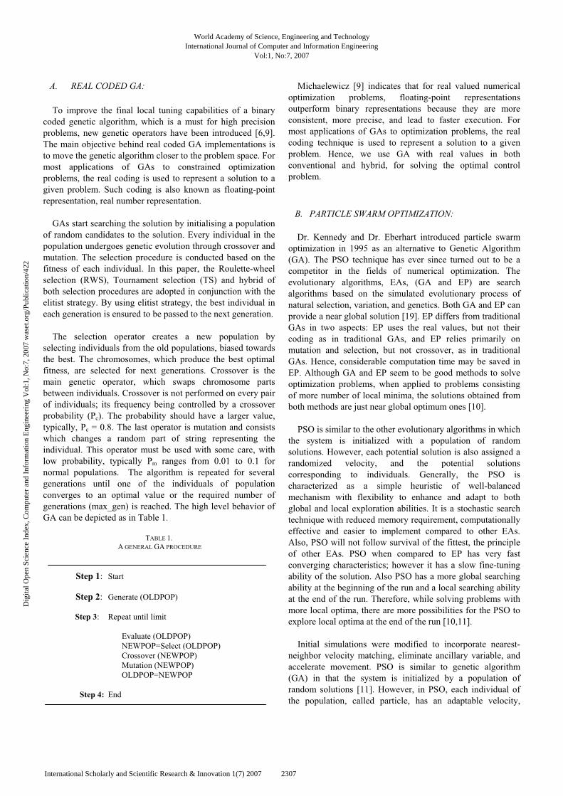
A. REAL CODED GA:

To improve the final local tuning capabilities of a binary

coded genetic algorithm, which is a must for high precision

problems, new genetic operators have been introduced [6,9].

The main objective behind real coded GA implementations is

to move the genetic algorithm closer to the problem space. For

most applications of GAs to constrained optimization

problems, the real coding is used to represent a solution to a

given problem. Such coding is also known as floating-point

representation, real number representation.

GAs start searching the solution by initialising a population

of random candidates to the solution. Every individual in the

population undergoes genetic evolution through crossover and

mutation. The selection procedure is conducted based on the

fitness of each individual. In this paper, the Roulette-wheel

selection (RWS), Tournament selection (TS) and hybrid of

both selection procedures are adopted in conjunction with the

elitist strategy. By using elitist strategy, the best individual in

each generation is ensured to be passed to the next generation.

The selection operator creates a new population by

selecting individuals from the old populations, biased towards

the best. The chromosomes, which produce the best optimal

fitness, are selected for next generations. Crossover is the

main genetic operator, which swaps chromosome parts

between individuals. Crossover is not performed on every pair

of individuals; its frequency being controlled by a crossover

probability (Pc). The probability should have a larger value,

typically, Pc = 0.8. The last operator is mutation and consists

which changes a random part of string representing the

individual. This operator must be used with some care, with

low probability, typically Pm ranges from 0.01 to 0.1 for

normal populations. The algorithm is repeated for several

generations until one of the individuals of population

converges to an optimal value or the required number of

generations (max_gen) is reached. The high level behavior of

GA can be depicted as in Table 1.

TABLE 1.

A GENERAL GA PROCEDURE

Step 1: Start

Step 2: Generate (OLDPOP)

Step 3: Repeat until limit

Evaluate (OLDPOP)

NEWPOP=Select (OLDPOP)

Crossover (NEWPOP)

Mutation (NEWPOP)

OLDPOP=NEWPOP

Step 4: End

Michaelewicz [9] indicates that for real valued numerical

optimization problems, floating-point representations

outperform binary representations because they are more

consistent, more precise, and lead to faster execution. For

most applications of GAs to optimization problems, the real

coding technique is used to represent a solution to a given

problem. Hence, we use GA with real values in both

conventional and hybrid, for solving the optimal control

problem.

B. PARTICLE SWARM OPTIMIZATION:

Dr. Kennedy and Dr. Eberhart introduced particle swarm

optimization in 1995 as an alternative to Genetic Algorithm

(GA). The PSO technique has ever since turned out to be a

competitor in the fields of numerical optimization. The

evolutionary algorithms, EAs, (GA and EP) are search

algorithms based on the simulated evolutionary process of

natural selection, variation, and genetics. Both GA and EP can

provide a near global solution [19]. EP differs from traditional

GAs in two aspects: EP uses the real values, but not their

coding as in traditional GAs, and EP relies primarily on

mutation and selection, but not crossover, as in traditional

GAs. Hence, considerable computation time may be saved in

EP. Although GA and EP seem to be good methods to solve

optimization problems, when applied to problems consisting

of more number of local minima, the solutions obtained from

both methods are just near global optimum ones [10].

PSO is similar to the other evolutionary algorithms in which

the system is initialized with a population of random

solutions. However, each potential solution is also assigned a

randomized velocity, and the potential solutions

corresponding to individuals. Generally, the PSO is

characterized as a simple heuristic of well-balanced

mechanism with flexibility to enhance and adapt to both

global and local exploration abilities. It is a stochastic search

technique with reduced memory requirement, computationally

effective and easier to implement compared to other EAs.

Also, PSO will not follow survival of the fittest, the principle

of other EAs. PSO when compared to EP has very fast

converging characteristics; however it has a slow fine-tuning

ability of the solution. Also PSO has a more global searching

ability at the beginning of the run and a local searching ability

at the end of the run. Therefore, while solving problems with

more local optima, there are more possibilities for the PSO to

explore local optima at the end of the run [10,11].

Initial simulations were modified to incorporate nearest-

neighbor velocity matching, eliminate ancillary variable, and

accelerate movement. PSO is similar to genetic algorithm

(GA) in that the system is initialized by a population of

random solutions [11]. However, in PSO, each individual of

the population, called particle, has an adaptable velocity,


Vol:1, No:7, 2007


Dig

ital O

pen

Scie

nce

Inde

x, C

ompu

ter

and

Info

rmat

ion

Eng

inee

ring

Vol

:1, N

o:7,

200

7 w

aset

.org

/Pub

licat

ion/

422

according to which it moves over the search space. Each

particle keeps track of its coordinates in hyperspace, which are

associated with the solution (fitness) it has achieved so far

[12]. This value is called personal best and is denoted by

pbest. Additionally among these personal bests, there is only

one, which has the best fitness. In a search space of D-

dimensions, the ith particle can be represented by a

vectorDi XXXX ,...,, 21

. Similarly, the relevant velocity is

represented by another D-dimensional vectorDi VVVV ,...,, 21

.

The best among pbest is called the global best, gbest.

(7))()()()( 2211 iiii XpbestrXgbestrwVV

In equation (7), w is known as the inertia weight. The best-

found position for the given particle is denoted by pbest and

gbest is the best position known for all particles. The

parameters 1 and 2 are set to constant values, which are

normally given as 2 whereas r1 and r2 are two random

values, uniformly distributed in [0, 1]. The position of each

particle is updated every generation. This is done by adding

the velocity vector to the position vector, as described in

equation (8) below: (8)iii VXX

The PSO algorithm, which is used in this paper to solve the

optimal control problem, is shown in table 2

TABLE 2.

PSO ALGORITHM

Step 1: Initialize

Set index of Global best (Gbest index) = 1;

Step 2: Create population

Randomize the positions and velocities for

entire population

Set the reference value of best position

PB (i). Fitness

Update velocity vector

Step 3: Calculate P (i). Fitness

If P (i). Fitness < reference value of best

position PB (i). Fitness

Then Set new reference value of best position

as P (i). Fitness

If PB (i). Fitness < PB (GBestIndex). Fitness

Then Set new GBestIndex = I

Step 4: Calculate the particle velocity and update the

particle positions using the Eqns. (6) and (7)

Step 5: Repeat until Maximum number of generation is

reached

The simplest version of PSO lets every individual move

from a given point to a new one which is a weighted

combination of the best position ever found (“nostalgia”), and

of the individual’s best position, pbest. The choice of the PSO

algorithm’s parameters (such as the group’s inertia) seems to

be of utmost importance for the speed and efficiency of the

algorithm [13 – 15]. Inertia weight plays an important role in

the convergence of the optimal solution to a best optimal

value as well as the execution time of the simulation run. The

inertia weight controls the local and global exploration

capabilities of PSO [10]. Large inertia weight enables the PSO

to explore globally and small inertia weight enables it to

explore locally. So the selection of inertia weight and

maximum velocity allowed may be problem – dependent. The

use of inertia weight, which typically decreases linearly, has

provided improved performance in optimal control problems.

IV. SELECTION OF GENETIC OPERATORS AND PSO

PARAMETERS

The main elements of a real coded GA include initial

population, fitness function, genetic operators (selection,

crossover and mutation), genetic structure, parameters

(max_gen, Pc, and Pm) etc. For PSO, the parameters used in

the algorithms are population size, population dimensions,

maximum generations, inertia weight and search space.

A. Initial population

The initial populations are generated randomly. And the

number of chromosomes generated per population is equal to

the dimension of the optimal problem or equal to the number

of jobs (N) involved in the main objective function. In this

paper, the number of chromosomes generated per population

(or the dimension of the optimal control problem) varies from

10 to 50.

B. Selection

Three different types of selection methods are used in this

paper: Roulette wheel method, Tournament selection method,

and the hybrid combinations with different proportions of

roulette wheel and tournament selection methods.

1) Roulette Wheel Selection Method

Each individual in the population is assigned a space on the

roulette wheel, which is proportional to the individual relative

fitness. Individuals with the largest portion on the wheel have

the greatest probability to be selected as parent generation for

the next generation.


Vol:1, No:7, 2007


Dig

ital O

pen

Scie

nce

Inde

x, C

ompu

ter

and

Info

rmat

ion

Eng

inee

ring

Vol

:1, N

o:7,

200

7 w

aset

.org

/Pub

licat

ion/

422

2) Tournament Selection Method

In tournament selection, a number Tour of individuals are

chosen randomly from the population and the best individual

from this group is selected as a parent. This process is

repeated to choose individuals often. These selected parents

produce uniform offspring at random. The parameter for this

method is the tournament size Tour. Tour takes values ranging

from 2 - Nind (number of individuals in population).

3) Hybrid Selection Method

The hybrid slection method consists of the combination of

both RWS and TS. We designed the hybrid selection

operation as a single level hybrid selection method. In this

technique, 50% of the population size adopts TS procedure

where as the RWS procedure is used in the remaining 50% of

the population size. For example, if we set population size as

20 then first 10 chromosomes follow TS method and the next

10 chromosomes follow RWS method.

C. Crossover

Crossover is the main genetic operator and consists of

swapping chromosome parts between individuals. Crossover

is not performed on every pair of individuals; its frequency

being controlled by a crossover probability (Pc). There are

several crossover methods available, but here we use hybrid

combination of Arithmetic crossover method (AMXO), and

Average Convex crossover (ACXO).

1) Arithmetic Crossover Method (AMXO)

The basic concept of this method is borrowed from the

convex set theory [5,8,9]. Simple arithmetic operators are

defined with the combination of two vectors (chromosomes)

as follows:

(9)1 yxx

(10)1 yxx

where is a uniformly distributed random variable between

0 and 1.

2) Average Convex Crossover Method (ACXO)

Generally, the weighted average of two vectors x1 and x2

are calculated as follows:

(11)2211 xx

If the multipliers are restricted as

(12)00,,1 2121

The weighted form (11) is known as convex combination.

Similarly, arithmetic operators are defined as the

combination of two chromosomes as follows:

(13)12211

22111

xxx

xxx

According to the restriction of multipliers, it yields three

kinds of crossovers, which can be called convex crossover,

affine crossover, and linear crossover. Among the three

methods, convex crossover may be the most commonly used

method [5]. When restricting 1 = 2 = 0.5, it yields a special case,

which is called as Average convex crossover by Davis or

Intermediate crossover by Schwefel [9].

3) Hybrid Crossover Methods

In this paper we designed four hybrid crossover methods

from the above said two crossover operations (AMXO and

ACXO). In the hybrid cross-over method, 50% of the

population size adopts AMXO procedure where as the ACXO

procedure is used in the remaining 50% of the population size.

We used some other crossover methods like direction based

crossover, single point crossover but the above said two

methods outperform all the other, hence we choose AMXO

and ACXO for hybrid method.

In

D. Mutation

The final genetic operator is Mutation. It can create a new

genetic material in the population to maintain the population’s

diversity. It is nothing but changing a random part of string

representing the individual. In this paper, dynamic mutation is

used.

1) Dynamic Mutation

Michalewicz [9] proposed this mutation operator, also

known as non-uniform mutation. It is designed for fine-tuning

capabilities aimed at achieving high precision. For a given

parent x, the element xk is randomly selected from the

following two possible choices:

(14),

,

L

kkkk

k

U

kkk

xxtxxor

xxtxx

The function (t, dx) returns a value in the range [0, dx]

such that the value of (t, dx) approaches 0 as t increases.

This property causes the operator to search the space

uniformly initially (when t is small) and very locally at later

stages. The function (t, dx) is given as follows:

(15))1(),( d

Ttrdxdxt

where r is a random number from (0,1), T is the maximal

generation number and d is a parameter determining the

degree of non-uniformity (usually assumed as 2 or 3).


Vol:1, No:7, 2007


Dig

ital O

pen

Scie

nce

Inde

x, C

ompu

ter

and

Info

rmat

ion

Eng

inee

ring

Vol

:1, N

o:7,

200

7 w

aset

.org

/Pub

licat

ion/

422

E. Elitism

In order to enrich the future generations with specific

genetic information of the parent with best fitness from the

current generations, that particular parent with the best fitness

is preserved in the next generations. This method of

preserving the elite parent is called elitism. This property is

incorporated in our proposed algorithms.

F. Population Size

From the earlier research, done by Shi, in 1998, it is proved

that the performance of the standard algorithm is not sensitive

to the population size. Based on these results the population

size in the experiments was fixed at 20 particles in order to

keep the computational requirements low. The size of the

population will affect the convergence of the solution. Hence

we set population size to 20 in our work.

G. Search Space

The range in which the algorithm computes the optimal

control variables is called search space. The algorithm will

search for the optimal solution in the search space which is

between 0 an d1. When any of the optimal control value of

any particle exceeds the searching space, the value will be

reinitialized. In this paper the lower boundary is set to zero (0)

and the upper boundary to one (1).

H. Dimension

The dimension is the number of independent variables,

which is identical to the number of jobs considered for

processing in the hybrid system framework. In this paper, the

dimension of the optimal control problem varies between 10

and 50.

I. Max Generations

This refers to the maximum number of generations allowed

for the fitness value to converge with the optimal solution. We

set 1000 generations for the simulation.

J. Inertia Weight

When the inertia weight is high (>0.7), the convergence rate

is faster but the optimal solution is not so optimal, but for the

lower value of inertia weight (<0.7), the convergence rate is

slower but the optimal solution is better. The monotonically

decreasing inertia weight from a higher value to a lower value

yields the better optimal solution with faster convergence. We

used all three categories in our algorithms to compare the

effect of inertia weight. In the monotonically decreasing

inertia weight technique, the first generation is simulated with

the higher value of inertia weight say 0.7, and the last

generations with lower inertia weight 0.3. So from generation

1 to 1000, the inertia weight also decreases from 0.7 to 0.3.

K. Solution acceleration technique

The convergence of the real coded GA can be accelerated

greatly by assuming that the best solution in the population is

closest to the global optimum. If it is true, then searching the

solution space in this neighborhood will produce solutions

closer to the global optimum. This can be accomplished by re-

mapping the population after each competition stage in the

GA algorithm so that all solutions are moved a random

distance towards the best solution at that generation. This

results in more solutions in the neighborhood of the minimum

and hence allows a more thorough search of its surrounds

[16].

Mathematically, the solution acceleration technique, which

is given in (16), can be described as follows:

(16)xxrxx bb

where xb = best solution vector (best individual) in

the population

x = solution vector (individual) to be re-

mapped

x’ = re-mapped solution vector

r = uniformly distributed random number

between 0 and 1.

V. TWO PHASE HYBRID GENETIC ALGORITHM (HRCGA):

The major difference that hybrid GAs can make regarding

performance enhancement is that they can provide an

acceptable solution within a relatively short time. In general,

local search techniques have the advantage of solving the

problem quickly, though their results are very much

dependent on the initial starting point; therefore, they can

easily be trapped in a local optimum. On the other hand,

genetic algorithm samples a large search space, climbs many

peaks in parallel, and is likely to lead the search towards the

most promising area. However, a GA faces difficulties in a

fine-tuning of local search; it spends most of the time

competing between different hills, rather than improving the

solution along a single hill that the optimal point locates.

Hence, if one can make use of the advantages of both the local

and GA techniques, one can improve the search algorithm

both effectively and efficiently [6, 9, and 17].

The proposed hybrid GA combines a standard real coded

GA and the phase - 2 of conventional search technique. Real

coded GA takes the place of the phase - 1 of the search [6, 9],


Vol:1, No:7, 2007


Dig

ital O

pen

Scie

nce

Inde

x, C

ompu

ter

and

Info

rmat

ion

Eng

inee

ring

Vol

:1, N

o:7,

200

7 w

aset

.org

/Pub

licat

ion/

422

providing the potential near optimum solution, and the

phase - 2 of a search technique using optimization by direct

search and systematic reduction in size of the search region

[18]. Phase - 2 algorithm is applied to rapidly generate a

precise solution under the assumption that the evolutionary

search has generated a solution near the global optimum.

A. Phase – 1 Algorithm

Real coded GA is implemented as follows:

1) A population of Np trail solutions is initialized. Each

solution is taken as a real valued vector with their dimensions

corresponding to the number of variables. The initial

components of x are selected in accordance with a uniform

distribution ranging between 0 and 1.

2) The fitness score for each solution vector x is evaluated

using Eq. 4, after converting each solution vector into

corresponding problem variables xa using upper and lower

bound vectors.

3) Three different (RWS, TS and Hybrid) selection method

are used individually to produce Np offspring from parents.

4) Hybrid crossover (combination of Arithmetic crossover

and Average crossover), non-uniform mutation operators and

solution acceleration technique are applied to offspring to

generate next generation parents.

5) The algorithm proceeds to step 2, unless the best solution

does not change for a pre - specified interval of generations.

Specifically, the phase - 1 of the hybrid algorithm stops if the

following condition of eqn.17 is satisfied: for the feasible best

solution vector at generation t, x[t], and generation t-1, x[t-1],

(17)11

tx

txtx

j

jj

for a sufficiently small positive value 1, and for all j, for

successive Ng1 generations.

B. Phase - 2 Algorithm

After the phase - 1 is halted, satisfying the halting condition

described in the previous section, optimization by direct

search and systematic reduction in size of the search region

method is employed in the phase - 2. In the light of the

solution accuracy, the success rate, and the computation time,

the best solution vector obtained form the phase - 1 is used

as an initial point for the phase - 2.

The optimization procedure based on direct search and

systematic reduction in search region is found effective in

solving various problems in the field of non-linear

programming. This procedure handles either inequality or

equality constraints or the feasible region does not have to be

convex and no approximations or auxiliary variables are

required. The most attractive features are the ease of setting

up the problem on the computer, speed in obtaining the

optimum and reliability of the results. For problems where

more than one local optimum can occur, this method is

especially useful [18]. This direct search optimization

procedure is implemented as follows:

1. The best solution vector obtained from the phase - 1 of

the hybrid algorithm is used as an initial point x(0) for

phase - 2 and an initial range vector is defined as

(18)*0 RangeRMFR

where Range is defined as the difference between the upper

and lower bound vectors of x and RMF is the range

multiplication factor. The RMF value varies between 0 and

1. In general, the value of RMF may be selected around 0.5 as

discussed in simulation results section.

2. Generate Ns trail solution vectors around x(0) using

following relationship,

(19),1*.00 nrandRxxi

where xi is ith trail solution vector, .* represents element-by-

element multiplication operation and rand (1,n) is a random

vector, whose elements value varies from 0 to 1.

3. For each feasible trail solution vector find the objective

function value using eqn.1 and find the trail solution set,

which minimizes f (x) and equate it to x(0).

(20)0 Bestxx

where xbest is the trail solution set with minimum f(x) for

minimization problems and maximum f(x) for maximization

problems.

4. Reduce the range by an amount given by

(21)1*00 RR

where is the range reduction factor, whose typical value is

0.02 or 0.05.

5. The algorithm proceeds to step2, unless the best solution

does not change for a pre - specified interval of iterations or

maximum number of iterations reached.

The main reason for the success of this algorithm lies in its

local search ability. Since the values for the variables are

always chosen around the best point determined in the

previous iteration, there is a more likelihood of convergence

to the optimum solution. In contrast, GAs spends most of the

time competing between different hills, rather than improving

the solution along a single hill that the optimal point locates.


Vol:1, No:7, 2007


Dig

ital O

pen

Scie

nce

Inde

x, C

ompu

ter

and

Info

rmat

ion

Eng

inee

ring

Vol

:1, N

o:7,

200

7 w

aset

.org

/Pub

licat

ion/

422

VI. NUMERICAL EXAMPLE, SIMULATION RESULTS

AND STATISTICAL ANALYSES

In order to compare the validity and usefulness of the

proposed hybrid real coded GA method, we considered the

optimal control problem from equations (5) and (6) with the

following functions:

(22)5.1*3,2

andxxu

u ii

i

ii

Now equation (5) becomes,

(23)3u

2

,....,

min1.5

1 i1

N

i

i

N

xJuu

(24)),max( )1( iiii uaxxsubjectto

The optimal controls (ui) and cost or fitness (J) for the

objective function given in equation (22) are computed with

the following parameter settings.

The dimension or the number of jobs involved in the

objective function N = (10,20,30,40,50), Crossover

probability Pc = 0.8 and Probability of mutation Pm = 0.01.

The maximum number of generations is set as 1000 with the

population size of 20.

The arrival sequence (ai for i = 1 to N) for N = (10, 20, 30,

40, 50), are obtained from the following algorithm given in

Table 3.

TABLE 3.

ARRIVAL SEQUENCE FOR HYBRID SYSTEMS.

ab(1) = 0.3

ab(2) = 0.5

ab(3) = 0.7

ab(4) = 1

For bb = 1 To N/4

For aa = 1 To 4

ab(aa + 4 * bb) = ab(aa) + 1 * bb

Next aa

Next bb

For i = 1 To N

a(i) = ab(i)

Next i

The number of arrival times, (ai for i = 1 to N) is taken

according to the dimension of the problem, i.e, the number of

jobs (N) considered for processing.

We solved the optimal control problem considered in this

section, which is given in equations (22 - 24) using three

proposed 2 phase hybrid GA methods. The proposed

algorithm adopts roulette wheel selection and the second

adopts tournament selection and the third provides hybrid of

both selection techniques.

We used a hybrid cross over technique, with arithmetic

cross-over (AMXO) and average cross – over (ACXO)

methods. The dynamic mutation is the unique choice of

mutation operation.

In order to compare the efficacy and validity, and to prove

the betterment of the proposed two- phase HRCGA method,

we solved the same optimal problem described in this section

through three PSO techniques (differs from each other with

inertia weight), and three conventional RCGA methods

(differs from each other with the selection procedure adopted).

All the above nine methods, given in Table (4), are

simulated 1000 times at different intervals of time, and their

statistical analyses are obtained. The Mean or average of the

fitness value obtained in 1000 runs and their Standard

Deviation (SD) are the basic statistical tests. From these two,

we calculated the Co-efficient of Variance (CV), which is the

ratio of standard deviation to Mean. The fourth statistical test

is Average Deviation (AVEDEV), which will give the average

of the absolute deviation of the fitness values from their mean,

which are taken in 1000 simulation runs. The graphical

comparisons of standard deviation and Average deviation of

the fitness value over 1000 runs for N = 10 to 50 are shown in

Fig 8(a-e). Added to these basic analyses, hypothesis t – test

and analysis of variance (ANOVA) test also were carried

out to validate the efficacy of all the nine methods. These

statistics analysis are presented in Tables 5 – 9. The graphical

analyses are done through Box plot, which are shown in

Figures 5 (a-e).

A box plot, which is shown in Figure 4, provides an

excellent visual summary of many important aspects of a

distribution. The box stretches from the lower hinge (defined

as the 25th percentile) to the upper hinge (the 75th percentile)

and therefore contains the middle half of the scores in the

distribution. The median is shown as a line across the box.

Therefore 1/4 of the distribution is between this line and the

top of the box and 1/4 of the distribution is between this line

and the bottom of the box.

The nth percentile of a distribution of values is defined as

the cumulative probability in percent, that is the value that

bounds the n% of values below and the (100-n)% above it. In

this report the box plot consists of a plot where 25th, 50th, and

75th percentiles are drawn. Looking at the box plot the general

features of the distribution can be evinced. For instance, if all


Vol:1, No:7, 2007


Dig

ital O

pen

Scie

nce

Inde

x, C

ompu

ter

and

Info

rmat

ion

Eng

inee

ring

Vol

:1, N

o:7,

200

7 w

aset

.org

/Pub

licat

ion/

422

Figure 4. A simple Box Plot

the percentiles of the model that are drawn in the box plot are

lower than the percentiles of the corresponding

measurements,. It means that the lower 75 % of the

predictions is lower than the lower 75 % of measurements.

This might probably correspond to a modeled distribution

everywhere lower than the measured one or, less likely, to a

model distribution much more peaked in the 25 (or less) % of

higher values.

Table 4 gives the description of all the nine methods

considered in this paper. The methods are classified according

to the optimization algorithm used to compute the optimal

control of the objective function. The above programes were

developed both in MATLAB 6.1 and Visual Basic 5.0

software packages.

For the purpose of comparison, we have considered our

earlier work on particle swarm optimization (PSO) and real

coded GA. All the methods are analyzed through hypothesis

test and finally by fitness regulation of the other methods over

the best method among all the nine methods.

TABLE 4.

VARIOUS OF THE EVOLUTIONARY OPTIMIZATION ALGORITHMS

S.No. Type of EA Methods Description

PSO - 1 PSO with high inertia weight (I.W = 0.7)

Particle Swarm

1 Optimization PSO - 2 PSO with low inertia weight (I.W = 0.3)

(PSO)

PSO - 3 PSO with monotonically decreasing inertia weight from 0.7 to 0.3

RCGA_RWS RCGA with roulette wheel selection, dynamic mutation

and hybrid cross over

Conventional

2 Real coded RCGA_TS RCGA with Tournament selection, dynamic mutation

Genetic Algorithm and hybrid cross over

(C RCGA)

RCGA_HGO RCGA with hybrid selection ( RWS + TS), dynamic mutation

and hybrid cross over

HRCGA_RWS Proposed 2 phase HRCGA with roulette wheel selection

dynamic mutation and hybrid cross over

Proposed 2 phase

3 Hybrid Real coded HRCGA_TS Proposed 2 phase HRCGA with Tournament selection,

Genetic Algorithm dynamic mutation and hybrid cross over

(HRCGA)

HRCGA_HGO Proposed 2 phase HRCGA with hybrid selection,

dynamic mutation and hybrid cross over


Vol:1, No:7, 2007


Dig

ital O

pen

Scie

nce

Inde

x, C

ompu

ter

and

Info

rmat

ion

Eng

inee

ring

Vol

:1, N

o:7,

200

7 w

aset

.org

/Pub

licat

ion/

422

TABLE 5.

STATISTIC ANALYSES OF FITNESS VALUE FOR N = 10

Method No. Statistical Test Average SD CV AVEDEV T-TEST for N = 10

1 PSO - 1 423.54124 0.56570 0.00134 0.38957 Method Nos. P Value Best Method

2 PSO - 2 414.37031 0.00000 0.00000 0.00000 1 & 2 1.0000 2

3 PSO - 3 414.37031 0.00000 0.00000 0.00000 2 & 3 0.9994 2

4 RCGA_RWS 423.02521 0.48518 0.00115 0.36491 2 & 4 0.0000 2

5 RCGA_TS 415.97974 0.33882 0.00081 0.29353 2 & 5 0.0000 2

6 RCGA_HGO 415.37357 0.22958 0.00055 0.16616 2 & 6 0.0000 2

7 HRCGA_RWS 414.37030 0.00001 0.00000 0.00000 2 & 7 0.0000 2

8 HRCGA_TS 414.37030 0.00001 0.00000 0.00000 2 & 8 1.0000 8

9 HRCGA_HGO 414.37030 0.00001 0.00000 0.00000 8 & 9 0.9998 9

Fig 5(a) ANOVA t – test for N = 10

Fig 7(a) Convergence of Fitness value over generations

for RCGA algorithms for N = 10

Fig 6(a) Convergence of Fitness value over generations

for PSO algorithms for N = 10

Fig 8(a) Convergence of Fitness value over generations for

proposed HRCGA algorithms for N = 10

1 2 3 4 5 6 7 8 9414

416

418

420

422

424

ANOVA t- Test for N = 10

Fitn

ess

Method Number

Convergnece of Fitness for PSO Algorithms

410

420

430

440

450

460

470

480

490

0 200 400 600 800 1000 1200

Number of Generations

Fitenss

PSO -1

PSO - 2

PSO - 3

Convergence of Fitness for Real Coded GAs

414.5

419.5

424.5

429.5

434.5

439.5

444.5

449.5

454.5

0 200 400 600 800 1000 1200


Fitn

ess

RCGA_RWS

RCGA_TS

RCGA_HGO

Convergence of Fitness for Hybrid Real Coded GAs

414.3702

414.3704

414.3706

414.3708

414.371

414.3712

414.3714

414.3716

0 200 400 600 800 1000 1200


Fitn

ess

HRCGA_RWS

HRCGA_TS

HRCGA_HGO


Vol:1, No:7, 2007


Dig

ital O

pen

Scie

nce

Inde

x, C

ompu

ter

and

Info

rmat

ion

Eng

inee

ring

Vol

:1, N

o:7,

200

7 w

aset

.org

/Pub

licat

ion/

422

TABLE 6.


Method No. Statistical Test Average SD CV AVEDEV T-TEST for N = 20


2 PSO - 2 1331.29258 0.28106 0.00021 0.24329 1 & 2 1.0000 2

3 PSO - 3 1331.08606 0.17978 0.00014 0.14429 2 & 3 0.9994 3

4 RCGA_RWS 1381.55553 0.69174 0.00050 0.39690 3 & 4 0.0000 3

5 RCGA_TS 1361.19747 0.79200 0.00058 0.63184 3 & 5 0.0000 3

6 RCGA_HGO 1356.81273 0.41574 0.00031 0.31490 3& 6 0.0000 3

7 HRCGA_RWS 1331.60000 0.29361 0.00022 0.23853 3 & 7 0.0000 3

8 HRCGA_TS 1330.93667 0.05561 0.00004 0.05137 3 & 8 1.0000 8

9 HRCGA_HGO 1330.92667 0.05208 0.00004 0.04185 8 & 9 0.7625 9

Fig 5(b) ANOVA t – test for N = 20

Fig 7(b) Convergence of Fitness value over generations for

RCGA algorithms for N = 20

Fig 6(b) Convergence of Fitness value over generations

for PSO algorithms for N = 20

Fig 8(b) Convergence of Fitness value over generations

for proposed HRCGA algorithms for N = 20

1 2 3 4 5 6 7 8 9

1330

1340

1350

1360

1370

1380

1390

ANOVA t - Test for N = 20

Fitn

ess

Method Number


1300

1400

1500

1600

1700

1800

1900

2000

0 200 400 600 800 1000 1200


Fitenss

PSO -1

PSO - 2

PSO - 3


1300

1350

1400

1450

1500

1550

1600

1650

1700

0 200 400 600 800 1000 1200


Fitn

ess

RCGA_RWS

RCGA_TS

RCGA_HGO


1330.5

1331

1331.5

1332

1332.5

1333

1333.5

1334

1334.5

0 200 400 600 800 1000 1200


Fitn

ess

HRCGA_RWS

HRCGA_TS

HRCGA_HGO


Vol:1, No:7, 2007


Dig

ital O

pen

Scie

nce

Inde

x, C

ompu

ter

and

Info

rmat

ion

Eng

inee

ring

Vol

:1, N

o:7,

200

7 w

aset

.org

/Pub

licat

ion/

422

TABLE 7.


Method No. Statistical Test Average SD CV AVEDEV T-TEST for N =30


2 PSO - 2 2805.24470 0.21571 0.00008 0.14058 1 & 2 1.0000 2

3 PSO - 3 2804.79883 0.14538 0.00005 0.10923 2 & 3 0.8007 3

4 RCGA_RWS 2898.92640 0.99552 0.00034 0.81273 3 & 4 0.0000 3

5 RCGA_TS 2880.37656 0.88922 0.00031 0.63029 3 & 5 0.0000 3

6 RCGA_HGO 2858.79713 0.79978 0.00028 0.51809 3& 6 0.0000 3

7 HRCGA_RWS 2807.00833 0.09841 0.00004 0.05982 3 & 7 0.0000 3

8 HRCGA_TS 2804.09877 0.06939 0.00002 0.06057 3 & 8 1.0000 8

9 HRCGA_HGO 2803.99745 0.05465 0.00002 0.03682 8 & 9 1.0000 9

Fig 5(c) ANOVA t – test for N = 30 Fig 6(c) Convergence of Fitness value over generations for

PSO algorithms for N = 30

Fig 7(c) Convergence of Fitness value over generations for


Fig 8(c) Convergence of Fitness value over generations for


1 2 3 4 5 6 7 8 92800

2820

2840

2860

2880

2900


Fitn

ess

Method Number


2700

3000

3300

3600

3900

4200

0 200 400 600 800 1000 1200


Fite

nss

PSO -1

PSO - 2

PSO - 3


2800

2900

3000

3100

3200

3300

3400

3500

3600

0 200 400 600 800 1000 1200


Fitness

RCGA_RWS

RCGA_TS

RCGA_HGO


2804

2806

2808

2810

2812

2814

2816

2818

2820

0 200 400 600 800 1000 1200


Fitness

HRCGA_RWS

HRCGA_TS

HRCGA_HGO


Vol:1, No:7, 2007


Dig

ital O

pen

Scie

nce

Inde

x, C

ompu

ter

and

Info

rmat

ion

Eng

inee

ring

Vol

:1, N

o:7,

200

7 w

aset

.org

/Pub

licat

ion/

422

TABLE 8.




2 PSO - 2 4915.58055 0.65593 0.00011 0.50865 1 & 2 1.0000 2

3 PSO - 3 4915.45251 0.62702 0.00013 0.50056 2 & 3 0.9829 3

4 RCGA_RWS 5006.66472 0.97196 0.00019 0.76077 3 & 4 0.0000 3

5 RCGA_TS 4987.95148 0.94147 0.00019 0.67175 3 & 5 0.0000 3

6 RCGA_HGO 4986.87711 0.88543 0.00018 0.61804 3& 6 0.0000 3

7 HRCGA_RWS 4924.22750 0.65949 0.00013 0.54541 3 & 7 0.0000 3

8 HRCGA_TS 4914.47004 0.53144 0.00011 0.43363 3 & 8 1.0000 8

9 HRCGA_HGO 4913.15394 0.52451 0.00011 0.39546 8 & 9 0.9934 9

Fig 5(d) ANOVA t – test for N = 40

Fig 7(d) Convergence of Fitness value over generations for


Fig 6(d) Convergence of Fitness value over generations for


Fig 8 (d) Convergence of Fitness value over generations for


1 2 3 4 5 6 7 8 9

4920

4940

4960

4980

5000

5020


Fitn

ess

Method Number


4700

5700

6700

7700

8700

9700

0 200 400 600 800 1000 1200


Fit

en

ss

PSO -1

PSO - 2

PSO - 3


4900

5100

5300

5500

5700

5900

6100

6300

0 200 400 600 800 1000 1200


Fit

ness

RCGA_RWS

RCGA_TS

RCGA_HGO


4910

4915

4920

4925

4930

4935

4940

0 200 400 600 800 1000 1200Number of Generations

Fit

ne

ss

HRCGA_RWS

HRCGA_TS

HRCGA_HGO


Vol:1, No:7, 2007


Dig

ital O

pen

Scie

nce

Inde

x, C

ompu

ter

and

Info

rmat

ion

Eng

inee

ring

Vol

:1, N

o:7,

200

7 w

aset

.org

/Pub

licat

ion/

422

TABLE 9.




2 PSO - 2 7744.00010 0.49792 0.00006 0.38174 1 & 2 1.0000 2

3 PSO - 3 7743.72344 0.49009 0.00006 0.37372 2 & 3 0.9830 3

4 RCGA_RWS 7761.02276 1.26549 0.00016 1.00445 3 & 4 0.0000 3

5 RCGA_TS 7759.42501 1.18389 0.00015 0.93502 3 & 5 0.0000 3

6 RCGA_HGO 7748.89319 0.99000 0.00013 0.71907 3& 6 0.0000 3

7 HRCGA_RWS 7744.62652 0.50900 0.00007 0.38848 3 & 7 0.0000 3

8 HRCGA_TS 7730.98000 0.49158 0.00006 0.37883 3 & 8 1.0000 8

9 HRCGA_HGO 7729.97667 0.42563 0.00006 0.28133 8 & 9 0.9937 9

Fig 5(e) ANOVA t – test for N = 50

Fig 7(e) Convergence of Fitness value over generations for






1 2 3 4 5 6 7 8 9

7730

7740

7750

7760

7770

7780


Fitn

ess

Method Number


7700

7900

8100

8300

8500

8700

8900

0 200 400 600 800 1000 1200


Fit

en

ss

PSO -3

PSO - 2

PSO -1


7500

8500

9500

10500

11500

12500

13500

14500

15500

16500

0 200 400 600 800 1000 1200


Fit

ne

ss

RCGA_RWS

RCGA_TS

RCGA_HGO


7730

7740

7750

7760

7770

7780

7790

0 200 400 600 800 1000 1200

Numeber of Generations

Fit

ne

ss

HRCGA_RWS

HRCGA_TS

HRCGA_HGO


Vol:1, No:7, 2007


Dig

ital O

pen

Scie

nce

Inde

x, C

ompu

ter

and

Info

rmat

ion

Eng

inee

ring

Vol

:1, N

o:7,

200

7 w

aset

.org

/Pub

licat

ion/

422

Fig 9(a) Comparison of SD and AVEDEV for N = 10

Fig 9(c) Comparison of SD and AVEDEV for N = 30

Fig 9(e) Comparison of SD and AVEDEV for N = 50

Fitness Regulation:

The percentage of deviation of the average fitness

value for the other eight methods from the best

among nine methods are calculated using equation

(25), for analyzing the better performance of the

proposed algorithm. They are presented in Table 10.

Fig 9(b) Comparison of SD and AVEDEV for N = 20

Fig 9(d) Comparison of SD and AVEDEV for N = 40

Fig 10. Percentage of Fitness value Regulation of other methods

from the best proposed method (HRCGA_HGO)

(25)

100_H

methodstherRCGA_HGO

%

HGORGAofFitness

oofFitnessHofFitness

valuefitnesstheofDeviationof

-0.10

0.00

0.10

0.20

0.30

0.40

0.50

0.60

1 2 3 4 5 6 7 8 9Method Number

Std

. D

ev &

A

ve. D

ev.

Standard

Deviation

Average

Deviation

0.00

0.10

0.20

0.30

0.40

0.50

0.60

0.70

0.80

0.90

1 2 3 4 5 6 7 8 9

Method Number

Std

. D

ev &

A

ve. D

ev.

Standard

Deviation

Average

Deviation

0.00

0.20

0.40

0.60

0.80

1.00

1.20

1 2 3 4 5 6 7 8 9

Method Number

Std

. D

ev &

A

ve. D

ev.

Standard

Deviation

Average

Deviation

0.00

0.20

0.40

0.60

0.80

1.00

1.20

1 2 3 4 5 6 7 8 9

Method Number

Std

. D

ev

&

A

ve

. D

ev

Standard

Deviation

Average

Deviation

-0.10

0.10

0.30

0.50

0.70

0.90

1.10

1.30

1.50

1 2 3 4 5 6 7 8 9

Method Number

Std

. D

ev &

A

ve. D

ev.

Standard

Deviation

Average

Deviation

-13.50

-11.50

-9.50

-7.50

-5.50

-3.50

-1.50

0.50

1 2 3 4 5 6 7 8

Method Number

F

i

t

n

e

s

s

R

e

g

u

l

a

t

i

o

n

N = 50

N = 40

N = 30

N =20

N = 10


Vol:1, No:7, 2007


Dig

ital O

pen

Scie

nce

Inde

x, C

ompu

ter

and

Info

rmat

ion

Eng

inee

ring

Vol

:1, N

o:7,

200

7 w

aset

.org

/Pub

licat

ion/

422

TABLE 10.

THE FITNESS VALUE REGULATION OF OTHER METHODS FROM THE BEST-PROPOSED METHOD (HRCGA_HGO)

No .of Jobs PSO - 1 PSO - 2 PSO - 3 RCGA_RWS RCGA_TS RCGA_HGO HRCGA_RWS HRCGA_TS

10 -2.2132 0.0000 0.0000 -2.0887 -0.3884 -0.2421 0.0000 0.0000

20 -4.5099 -0.0275 -0.0120 -3.8040 -2.2744 -1.9450 -0.0506 -0.0008

30 -3.6522 -0.0445 -0.0286 -3.3855 -2.7239 -1.9543 -0.1074 -0.0036

40 -1.1640 -0.0494 -0.0468 -1.9033 -1.5224 -1.5005 -0.2254 -0.0268

50 -0.6852 -0.1814 -0.1778 -0.4016 -0.3810 -0.2447 -0.1895 -0.0039

VII DISCUSSION AND CONCLUSIONS

In this paper, new two-phase hybrid real coded genetic

algorithms with hybrid genetic operators are proposed. This

algorithm (2-phase HRCGA) can out perform conventional

genetic algorithms and PSO in the sense that hybrid GAs

make it possible to improve both the quality of the solution

and reduce the computing expenses. The phase -1 uses

standard real coded genetic algorithm, while optimization

by direct search with systematic reduction in the size of the

search region is employed in the phase - 2. This hybrid

algorithm handles either inequality or equality constraints

and the feasible region does not have to be convex and

gradient or other auxiliary information’s are not required.

In order to prove the effectiveness of the proposed

algorithm, this method is applied to typical constrained

optimization function. The results obtained are compared

with other methods. The outcome of the study clearly

demonstrates the effectiveness and robustness that a hybrid

genetic algorithm (HGA) can achieve over a conventional

RCGA and PSO algorithms. From the results, it is very

clear that hybrid GA not only improves the success rate but

also decreases the number function evaluations and

computation time.

In this paper, three different evolutionary algorithms are

considered. Three algorithms for each of these three

methods, a total of nine methods are considered. In order

to compare the validity and usefulness of the proposed

hybrid real coded GA method with the other evolutionary

methods, 1000 simulated results for each method are taken

at different timings. In order to hasten the convergence in

hybrid real coded GA's solution and the population

dimension (Pop_Size), maximum of number of generation

(max_gen), are set to 20 and 1000 respectively. The

performance of different algorithms is compared with

respect to the solution accuracy in the fitness, the standard

deviations, co-efficient variance, average deviation,

ANOVA t-test, and the percentage of deviation in the

fitness from the proposed best method.

From the results stated in Table 5 – 9, it is obvious that

the method - 9 (HRCGA_HGO) is best followed by

method - 8 (HRCGA_TS). This clearly establishes the fact

that hybrid selections together with hybrid crossover

methods yield better solutions. This is the most significant

outcome of the experiments performed. These

combinations have been shown to work efficiently with

regard to an optimal control problem here but it is believed

that these might be equally efficient with regard to all other

problems where hybrid real coded GA can be used.

A. From the ANOVA test and t – test:

The hypothesis t – Test and ANOVA test are also carried

out to prove the best method among all the nine methods

considered here, and their P-values are also recorded. The

ANOVA test results are drawn using Box plots. From the

box plot figures, which are given in Fig 5 (a-e), it is

obvious that method - 9 (HRCGA_HGO) gives the best

results among all other methods. This clearly indicates that

the hybrid selection with the hybrid combination of AMXO

and ACXO gives the best results.

B. From the convergence of fitness graphs:

Fig. 6 (a-e), Fig 7(a-e), and Fig 8(a-e) show the

convergence characteristics of PSO, real coded and hybrid

real coded genetic algorithms respectively for number of

jobs N = 10, 20, 30, 40 and 50. It is clearly seen from the

graphs that the proposed two phase HRCGA methods

converge very earlier, around generation 200, which is not

so in other methods (see Fig 7(a-e)). PSO methods

convergences faster but only for less number of jobs. For

higher number of jobs, PSO also takes more number of

generations to converge with the final optimal value (see

Fig 5(a-e)). In the case of the conventional RCGA methods

(Fig 6(a-e)), the convergences of fitness value with the

optimal value take more number of generations, which will

in turn take longer computation time. It clearly shows the


Vol:1, No:7, 2007


Dig

ital O

pen

Scie

nce

Inde

x, C

ompu

ter

and

Info

rmat

ion

Eng

inee

ring

Vol

:1, N

o:7,

200

7 w

aset

.org

/Pub

licat

ion/

422

inefficiency of real coded GA in fine local tuning. If, for

the entire search, real coded GA were employed then there

would be a mere wastage of amount computation time

without any change in solution vector and objective

function value. Since the two phase HRCGA method

converges at less number of generations, this algorithm

takes less computation time in comparison to the other

methods in order to obtain the optimal solution.

C. From the SD and Average dev. Graph:

It is very obvious that the standard deviation and average

deviations are the quality measures of statistical analyses.

In order to obtain the optimal value of the fitness function,

the optimization algorithms were run 1000 times in

different intervals of time. If the algorithm gives nearly

same solution in each and every run, then we can say that

the algorithm is consistent and stable for solving the

optimal control problem.

In order to prove the consistency and stability on the

optimal solution, standard deviations and average

deviations of the fitness value are taken through the 1000

simulated runs. If the standard deviation is very minimum,

it implies that the solution obtained in each of 1000 runs are

more or less equal and the differences between the

solutions over each runs are less. Therefore, if an algorithm

provides very low standard deviation then it can be

concluded that the algorithm is consistent. From Fig 8 (a-e),

it is observed that method 9 provides a very low standard

deviation among all other methods.

The average deviation gives the measure of how much

the solution is deviated from the average (mean) value of

the fitness. For the algorithm to be on best side, it should

produce a very low average deviation. From Fig 8 (a-e), it

is very clearly seen that the 9th method gives a very low

average deviation. Hence we strongly conclude that the 9th

method is the best among the others.

D. From the Fitness regulation:

The same conclusions can also be drawn from Table 10,

where percentage of deviations of fitness values, called as

fitness regulation, were obtained through methods 1 to 8

from the proposed best method; method - 9 (HRCGA_HGO)

is recorded. For smaller number of jobs, method - 8

(HRCGA_TS) and method - 3 (PSO-3) also yield the

optimum value but when the numbers of jobs increase they

are differ from method - 9.

The graphical representation of this fitness regulation is

shown in Fig 10. The negative values of this fitness

regulation indicate that methods 1 – 8 are inferior to

method - 9. The zero fitness regulation for the particular

methods indicate that the optimum value is same with the

proposed best method - 9. Based on this, it can be

concluded that the hybrid real coded GA with the hybrid

genetic operators gives the best optimal value over the

other methods.

In other words, the superior performance of the hybrid

combinations of the genetic operators for two phase hybrid

real coded genetic algorithms has been clearly established

in this paper.

REFERENCES

[1] C.G. Cassandras, D.L.Pepyne, and Y.Wardi, “ Optimal Control of a

class of Hybrid Systems,” IEEE Trans. Automat.Cont., vol 46 pp.

398 – 415, Mar 2001. [2] Ping Zhang and Chris Cassandras, “An Improved Forward algorithm

for Optimal Control of a Class of Hybrid Systems” IEEE Trans.

Automat. Cont., vol 47, pp.1735-1739, October 2002.

[3] M.Senthil Arumugam, M.V.C.Rao, Tiew Ting On (2004) “A Novel

approach of Hybrid Selection for Real Coded Genetic Algorithm for

Computing Optimal Control of a class of Hybrid Systems”,

International Conference on Computational Intelligence (Accepted)

to be published.

[4] Kennedy, J. (1997), “The Particle Swarm: Social Adaptation of

Knowledge” Proc. IEEE international Conference on Evolutionary

Computation (Indianapolis, Indiana), IEEE service center,

Piscataway, NJ, 303 – 308.

[5] D. Goldberg, Genetic Algorithms in Search, Optimisation and

Machine Learning, Addison Wesley Massachusetts, USA 1989.

[6] Z. Michalewicz, Genetic Algorithms + Data Structures = Evolution

Programs, Springer Verlag 1994.

[7] S.Baskar, P.Subbaraj, M.V.C.Rao, “Performance of Hybrid Real

Coded Genetic Algorithms,” Intl. Journal of Computational

Engineering Science. 2, No. 4 (2001).

[8] L.Davis, A Hand Book of Genetic Algorithm, New York 1990.

[9] Mitsuo Gen and Runwei Cheng, Genetic Algorithms and

Engineering Design, John Wiley & Sons, Inc., 1997.

[10] Kennedy J., Eberhart, R.C.(1995), “Particle Swarm Optimization”,

Proc. IEEE international conference on Neural Networks (Perth,

Australia), IEEE service center, Piscataway, NJ, IV: 1942- 1948.

[11] R. C. Eberhart and Y. Shi, (1998) "Comparison between Genetic

Algorithms and Particle Swarm Optimization", Evolutionary

Programming VII (1998), Lecture Notes in Computer Science 1447,

pp. 611-616, Springer.

[12] P. J. Angeline, (1998) "Evolutionary Optimization versus Particle

Swarm Optimization: Philosophy and Performance Differences",

Evolutionary Programming VII (1998), Lecture Notes in Computer

Science 1447, pp. 601-610, Springer.

[13] Y. Shi and R. C. Eberhart, (1998) "Parameter Selection in Particle

Swarm Optimization", Evolutionary Programming VII (1998),

Lecture Notes in Computer Science 1447, pp. 591-600, Springer.

[14] . Shi and R.C. Eberhart, (1998) “A modified particle swarms

optimizer”. Proceedings of the IEEE International Conference on

Evolutionary Computation, Anchorage, Alaska, May 4-9.

[15] Y. Shi and R.C. Eberhart, (1999) “Empirical study of particle swarm

optimization”, Congress on Evolutionary Computation, Washington

D.C.,USA July 6-9

[16] K.P.Wong, A.li and M.Y.law, “Development of constrained-genetic-

algorithm load Flow methods “IEE proceedings- Generation

,Transmission and Distribution, vol 144, No.2, March 1997.

[17] F. Li R. Morgan and D.Williams, Hybrid genetic approaches to

ramping rate Constrained dynamic economic dispatch, Electric

power systems research vol43, 1997.

[18] Rein Luss and T.H.I. Jaakola, Optimization by direct search and

system reduction of the size of search region, AIChE Journal ,

Vol.19,No.4,1973.


Vol:1, No:7, 2007


Dig

ital O

pen

Scie

nce

Inde

x, C

ompu

ter

and

Info

rmat

ion

Eng

inee

ring

Vol

:1, N

o:7,

200

7 w

aset

.org

/Pub

licat

ion/

422

Novel Hybrid Approaches For Real Coded Genetic Algorithm To

Documents

Transcript of Novel Hybrid Approaches For Real Coded Genetic Algorithm To

Real Coded Quantum Genetic Algorithm and its Application · PDF fileReal Coded Quantum Genetic Algorithm and its Application ... proposes a new real number coded quantum genetic algorithm,

Real Coded Genetic Algorithm Approach to Harmonic ... · variable-voltage multilevel inverters that can operate over a wide range of modulation indices. In this paper, Real Coded

Pattern Synthesis using Real Coded Genetic Algorithmamsemodelling.com/publications/advances_in_modelling/Signal... · Pattern Synthesis using Real Coded Genetic Algorithm ... Antenna

Genetic Algorithm

Solving fluid flow problems using a real-coded genetic ... · Solving fluid flow problems using a real-coded genetic algorithm with uniform refinement R. Bourisli & D. A. Kaminski

A real-coded genetic algorithm for training recurrent ... · A real-coded genetic algorithm for training recurrent neural networks A. Blanco, M. Delgado, M.C. Pegalajar* Department

Genetic Algorithms (GAs) By Mutaz Flmban. Outline History of Genetic Algorithm What is the Genetic Algorithm Biological Background Basic Genetic Algorithm.

Use Genetic Algorithm in Optimization Function For … · Use Genetic Algorithm in Optimization Function ... And The Genetic Algorithm is well ... Use Genetic Algorithm in Optimization

CHAPTER 3 REAL CODED GENETIC ALGORITHM FOR FUZZY ...shodhganga.inflibnet.ac.in/bitstream/10603/25376/8/08_chapter3.pdf · REAL CODED GENETIC ALGORITHM FOR FUZZY CLASSIFIER DESIGN

J3 - Elsevier JOCS - a New Population Seeding Technique for Permutation-Coded Genetic Algorithm

Research Article Real-Coded Quantum-Inspired Genetic ...downloads.hindawi.com/journals/mpe/2015/571295.pdf · Research Article Real-Coded Quantum-Inspired Genetic Algorithm-Based

Binary-Real Coded Genetic Algorithm Based K-Means Clustering for ...

Real-Coded Genetic Algorithms - Purdue Engineeringsudhoff/ee630/Lecture04.pdfReal-Coded Genetic Algorithms. 2 Drawbacks of Binary Coded GAs Hamming cliffs Moving to a neighboring solution

Real-Coded Genetic Algorithm with Average-Bound Crossover ...

Tackling Real-Coded Genetic Algorithms

Real-Coded Genetic Algorithm Particle Filters for High ...discovery.ucl.ac.uk/1426733/1/PhD_Thesis_-_Muhammad_Shakir_Huss… · Real-Coded Genetic Algorithm Particle Filters ... Figure

Real Coded Genetic Algorithm Operators Embedded in ...€¦ · Gravitational Search Algorithm (GSA) is a new addition in the class of nature inspired optimization techniques based

Particle Swarm Optimization Algorithm vs Genetic …file.scirp.org/pdf/ICA20110400018_39934944.pdf · Both real-coded Genetic Algorithm and Particle Swarm Optimization are used to

Real-Coded Extended Compact Genetic Algorithm based on Mixtures of Models

Real-Coded Adaptive Range Genetic Algorithm And …flab.eng.isas.jaxa.jp/member/oyama/papers/jsme2000.pdfReal-Coded Adaptive Range Genetic Algorithm And Its Application to Aerodynamic