26

CHAPTER 3

REAL CODED GENETIC ALGORITHM FOR FUZZY

CLASSIFIER DESIGN

3.1 INTRODUCTION

Genetic Algorithm (GA) (Goldberg 1989) is a generalized search

and optimization technique inspired by the theory of biological evolution.

While many authors applied GA for system identification and control

problems, only a few authors have focused on data classification problems

and still there exist a number of issues in applying genetic algorithms for

designing the fuzzy classifier.

The conventional Binary-coded GA (BGA) has Hamming cliff

problem (Devaraj et al. 2005) which sometimes may cause difficulties in the

case of coding continuous variables. Also, for discrete variables with total

number of permissible choices not equal to 2k (where k is an integer), it

becomes difficult to use a fixed length binary coding to represent all

permissible values.

To overcome the above difficulty, this chapter presents Real- coded

GA (RGA) for fuzzy classifier design. It also discusses the issues to be

addressed in developing a Genetic Fuzzy classifier model.

27

No

Yes

Calculate fitness value

Select parents for reproduction

Apply crossover and mutation

Evaluate fitness of Chromosomes

Converged ?

Stop

N

Generate initial population

Start

3.2 OVERVIEW OF GENETIC ALGORITHM

Genetic Algorithm (Sivanandam, 2007) maintains a population of

individuals that represent candidate solutions. Each individual is evaluated to

give some measure of its fitness to the problem from the objective function. In

each generation, a new population is formed by selecting the more fit

individuals based on a particular selection strategy. Some members of the new

population undergo genetic operations to form new solutions.

Figure 3.1 Flowchart of Genetic Algorithm

The two commonly used operations are crossover and mutation.

Crossover is a mixing operator that combines genetic material from selected

parents. Mutation acts as a background operator and is used to search the

unexplored search space by randomly changing the values at one or more positions of the selected chromosome.

28

As shown in Figure 3.1, starting with an initial population, the

genetic algorithm exploits the information contained in the present population

and explores new individuals by generating offspring using the three genetic

operators namely, reproduction, crossover and mutation which can then

replace members of the old generation. Fitter chromosomes with higher

probabilities are selected for the next generation. After several generations,

the algorithm converges to the best chromosome, which hopefully represents

the optimum or near optimal solution.

3.3 REAL CODED GENETIC ALGORITHM

In a standard Simple Genetic Algorithm (SGA), binary strings are

used to represent the solution variables. It is widely recognized that the SGA

scheme is capable of locating the neighborhood of the optimal or near-optimal

solutions, but, in general, SGA requires a large number of generations to

converge. This is especially because of decoding of binary strings into real

numbers and vice versa. Moreover, this binary string makes GA to suffer

from the Hamming Cliff’s problem.

The Hamming cliff (Yu et al. 2010) is the phenomena that occurs

when the pair 0111111111 and 1000000000 belonging to neighboring points

in the phenotype space but have a maximum Hamming distance in the

genotype space. To cross this Hamming cliff all bits have to be changed

simultaneously. The probability of this to occur with crossover and mutation

is very small and results in premature convergence.

To overcome this difficulty, modifications are made in the

proposed Real-coded Genetic Algorithm (RGA) such that rule set is

represented using integer number and membership functions are represented

using floating point number. The power of GA lies in the kind of genetic

operators applied to modify the parameters of the chromosome and find the

29

better solutions to the problem. The following real parameter genetic

operators are popularly used in the literature for the RGA based fuzzy

classifier design.

Roulette wheel selection, Weighted mean cross over, Uniform

mutation are used by Russo et al. (2000).

Rank selection, Arithmetic cross over, Random mutation

(Setnes et al. 2000).

Roulette wheel selection, Max-min arithmetical crossover and

Uniform mutation are used by Casillas et al. (2005).

Tournament Selection, BLX-a crossover, Random mutation

are used by Alcala et al. (2007).

Tournament selection, Arithmetic crossover and Uniform

mutation are used by Devaraj et al. (2010).

In this research work, Tournament Selection, BLX-

Non-uniform mutation operations are used. The details of the genetic

operators are presented in the following subsections:

3.3.1 Tournament Selection

The goal of selection is to allow the “fittest” individuals to be

selected more often to reproduce. In tournament selection, ‘n’ individuals are

selected randomly from the population, and the best of the ‘n’ is inserted into

the new population for further genetic processing. Tournaments are often held

between pairs of individuals, although larger tournaments can be used. This

procedure is repeated until the mating pool is filled.

30

I

e2e1

u2u1

u min u max

3.3.2 BLX-

Crossover is a mixing operator that combines particle’s individual

best position from the randomly selected particles. BLX-

finds out a new position y from the space [ ], 21 ee as follows:

y = otherwisesamplingrepeat

uyuifeere:

: maxmin121 (3.1)

where, )( 1211 uuue (3.2)

1222 uuue (3.3)

:r Uniform random number 1,0

Figure 3.2 illustrates the BLX-

dimensional case. It is noted from the Figure 3.2 that e1 and e2 will lie

between minu and maxu , the variable’s lower and upper bound respectively. In a

number of trial runs, it i

Figure 3.2 BLX-

One interesting feature of this type of crossover operator is that the

created point depends on the location of both parents. If both parents are close

to each other, the new point will also be close to the parents. On the other

hand, if parents are far from each other, the search is more like a random search.

31

After the crossover, the fitness of the individual best position is

compared with that of the two offspring, and the best one is taken as the new

individual best position.

3.3.3 Non-uniform Mutation

Mutation is a varying operator that randomly changes the values at

one or more positions of the selected particle. In Non-uniform mutation, for

each chromosome mti xxxX ,...,, 21 in the population of t-th iteration, an

offspring mti xxxX ...,,, '

2'1

1 is produced as below:

1,,0,,'

israndomaifLBxtxisrandomaifxUBtx

xkk

kkk (3.4)

where LB and UB are the lower and upper bounds of the variables xk. The

function yt, returns a value in the range [0,y] such that yt, approaches

zero as t increases. This property causes this operator to search the space

uniformly at initial stages (when t is small), and very locally at later stages.

This strategy increases the probability of generating a new number

close to its successor than a random choice. The function yt, is evaluated

as below:

b

Tt

ryyt1

1., (3.5)

where r is a random number from [0,1], T is the maximum iteration, b is a

system parameter determining the degree of dependency on the iteration

number.

32

3.4 RGA IMPLEMENTATION

While designing an FLBCS using any population based stochastic

optimization techniques including RGA; the following issues are to be

addressed:

Representation of solution variables.

Formulation of Fitness function.

3.4.1 Representation

The first important consideration for designing an optimal FLBCS

is the representation strategy to be followed for the solution variables namely

rule set and membership function. A fuzzy system is said to be completely

specified only when the rule set and the membership function associated with

each fuzzy set are represented as a single individual.

3.4.1.1 Representation of MF

To represent the membership function, the range of each input

variable is partitioned into areas and then it is associated with fuzzy sets. In

general three to seven partitions are appropriate to cover the required range of

an input variable. Once the names of the fuzzy sets are determined, then their

associated membership functions are to be considered. In general, the shape

of the membership function depends on the nature of the problem. Piecewise

linear functions such as triangular or trapezoidal functions are widely used

membership functions in the fuzzy system design because of its simplicity

and sensibility.

In this research work, Trapezoidal membership function is used for

starting and ending fuzzy regions and Triangular membership function is used

33

0

P9 P8

P7 P6

P5

P3P4

P2P1

Variable Range

L HM

1

for intermediate fuzzy regions. After deciding the type of membership

function, the points required for placing them in the fuzzy space and their

ranges are computed as per the procedure illustrated using Figure 3.3.

Figure 3.3 Fuzzy Partitions

As shown in Figure 3.3, if the range of an input variable is

partitioned into three fuzzy sets namely, Low (L), Medium (M) and High (H),

then a total of nine membership points (P1, P2, P3, P4, P5, P6, P7, P8, P9) are

required for representing the input variable.

In that nine points, first and last points (P1 and P9) are fixed that are

the minimum and maximum of the input variable. The remaining seven

membership points are evolved between the dynamic range such that P2 has

[P1,P9], P3 has [P2,P9], P4 has [P2,P3], P5 has [P4,P9], P6 has [P5,P9], P7 has

[P5,P6] and P8 has [P7,P9] as limits.

As an extension of the above method if five fuzzy sets are used to

represent each variable, then a total of fifteen membership points (P1, P2, P3,

P4, P5, P6, P7, P8, P9, P10, P11, P12, P13, P14, P15) are required and has limits as

discussed for the three fuzzy sets.

34

3.4.1.2 Representation of Rule Set

Each rule in the rule set has three sections: rule selection (‘R’),

representation for the input variables (antecedent – I1, I2,…, In) and the

representation for the output classes (consequent – ‘O’). Rule selection may

take either ‘1’ to select the rule otherwise ‘0’.

If three fuzzy sets (low, medium and high) are used, then each

antecedent part may take an integer value ranges from 0 to 3 such that ‘0’

represents “don’t care”, ‘1’ represents “low”, ‘2’ represents “medium”, ‘3’

represents “high”. The output class is also represented by an integer value

whose range depends on the number of class labels.

With this idea, a typical rule set and membership function will be

represented as shown in Figure 3.4

0 1 2... 3 1 1 1 3… 2 4 … 0 3 2… 3 2

R I1 I2 In O R I1 I2 In O R I1 I2 In O

Rule 1 Rule 2 Rule MNR

5.6,6.1,7.0 2.6,3.2,3.8 2.4,3.9,5.4 … 0.3,0.6,0.9 1.2,1.5,1.8 2.4,2.7,3.1

L M H L M H

Input 1 Input n

Figure 3.4 Representation of Rule Set and Membership Function

This type of representation is simpler and can be extended to any

number of fuzzy sets.

35

3.4.2 Fitness Function Formulation

The next important consideration following the representation is the

formulation of fitness function. Evaluation of the individuals in the population

is accomplished by calculating the objective function value for the problem

using the parameter set. The result of the objective function calculation is

used to calculate the fitness value of the individual. In the classification

problem under consideration, there are two objectives:

1. Maximize the correctly classified data.

2. Minimize the number of rules.

These two objectives are conflicting objectives. This is overcome

by reformulating the first objective of maximizing the correctly classified data

as minimizing the difference between total number of samples and the

correctly classified data.

Given the total number of samples (‘S’) and the maximum number

of rules (‘MNR’), the task is to find out the difference between ‘S’ and the

correctly classified data (‘Cc’) for the selected number of rules(‘SNR’) and the

objective is to find out the minimum of this value. This is mathematically

represented as,

RSNkCcSfMin (3.6)

where ‘k’ is a constant introduced to amplify ‘SNR’ whose value is usually

small.

3.5 SIMULATION RESULTS

This section presents the details of the simulation carried out for ten

benchmark datasets available in the UCI machine learning repository

(Asuncion 2007) to demonstrate the effectiveness of the proposed RGA based

approach for Fuzzy Classifier Design.

36

The proposed approach is developed using Matlab R2009 and

executed in a PC with Pentium IV processor with 2.40 GHz speed and 256

MB of RAM. Experiments are conducted to examine both the learning ability

as well as the generalization ability of the proposed approach in the formation

of rule base and membership function.

3.5.1 Datasets

The details of ten benchmark datasets from four different

applications areas used in the simulation are given in Table 3.1. It shows, for

each dataset, the area, the number of attributes (#A), type of each attribute (T),

the number of classes (#C), total number of samples (#TS) and the number of

class wise samples (#CWS).

Table 3.1 Details of Dataset

Area Name # A Types # C #TS #CWS

Life Science

Breast Cancer 10 All are Integer 2 699 458,241 Pima Indians Diabetes 8 Integer (1,2,3,4,5,8)

Real (6,7) 2 768 500,268

Iris 4 All are Real 3 150 50,50,50

Ecoli 8 All are Real 8 336 143,77,52,35,20,5,2,2

Yeast 8 All are Real 10 1484 463, 429, 244, 163, 51, 44, 37, 30, 20, 5

Physical Science

Magic Gamma Telescope 11 All are Real 2 1902

0 12332, 6688

Wine 13Integer(1,6,13) Real(2,3,4,5,7,8,9,10,11,12)

3 178 59, 71, 48

Glass Identification 9 All are Real 6 214 70,17,76,

13,9,29

Financial Credit Approval 14

Categorical (1,4,5,6,7,9,10,12,13) Integer (3,11,14)Real (2,8)

2 690 307,383

Computer Page Blocks Classification 10 Integer (1,2,3,8,9,10)

Real (4,5,6,7) 5 5473 4913, 329, 28,88, 115

37

3.5.2 Learning Ability

First the learning ability of the proposed RGA is examined by using

all the samples of a dataset as training patterns. The details of the simulation

and the performance of the classifier for the Wine data are presented here.

The wine data contains the chemical analysis of 178 wines with 13

input variables and 3 output classes. As shown in Figure 3.3, each input

variable of the wine data is represented by three fuzzy sets namely, “low”,

“medium” and “high”. Trapezoidal membership function is used to represent

the “low” and “high” fuzzy sets. Triangular membership function is used to

represent the “medium” fuzzy set.

Seven points are required to represent an input variable and hence a

total of ninety one (13×7=91) membership function points are needed. Each

rule for a wine data set requires fifteen integer numbers (1 for rule selection +

13 for input variables + 1 for output class). A maximum of six rules are

included and hence a total of ninety integer numbers (6×15 =90) are needed

to represent the complete rule set.

The proposed approach is run with 30 independent trials with

different values of random seeds and control parameters.

Population Size : 30

Generations : 300

Tournament Size : 2

Crossover Probability : 0.8

Mutation Probability : 0.1

38

With the above settings, the convergence characteristics of the

proposed RGA in designing the FLBCS are analyzed.

0 50 100 150 200 250 3000

0.5

1

1.5

2

2.5

3

3.5

4Convergence of RGA

Iterations

Figure 3.5 Convergence of RGA for Wine dataset

It is found that for the first hundred generations, there is a faster

improvement in the fitness value, above that and up to two hundred

generations, its shows gradual improvements. Afterwards, the proposed RGA

steadily increases the fitness and reaches the optimal solution.

During the course of run, the ranges of each membership function

points are evolved and tuned at the same time. The values of membership

function points (P2 to P8) obtained finally for each variable after reaching the

optimal solution are recorded. Then using those points, the shape of the

membership function of each fuzzy set of a variable is analyzed. Figure 3.6

shows the membership function plotted for the variable magnesium of wine

dataset.

39

70 80 90 100 110 120 130 140 150 1600

0.1

0.2

0.3

0.4

0.5

0.6

0.7

0.8

0.9

1Input Varibale: Magnesium of Wine dataset

Variable Range

Figure 3.6 Membership Function obtained by RGA for Wine Dataset

The three near optimal rules evolved by the proposed RGA for

wine data set are given below.

If color intensity and alcohol are low and malic acid and ash

are medium and proline and flavanoid are high then it is wine

1.

If magnesium and color intensity are medium and malic acid

and Flavanoid are low and hue and ash are medium then it is

wine 2.

If ash and proline are low, and color intensity and total phenol

are high and alcohol and colour intensity are medium then it is

wine 3.

In order to show the usefulness of the proposed approach for a

medical diagnosis problem, the results obtained for Breast Cancer data set is

40

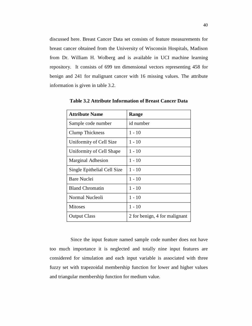
discussed here. Breast Cancer Data set consists of feature measurements for

breast cancer obtained from the University of Wisconsin Hospitals, Madison

from Dr. William H. Wolberg and is available in UCI machine learning

repository. It consists of 699 ten dimensional vectors representing 458 for

benign and 241 for malignant cancer with 16 missing values. The attribute

information is given in table 3.2.

Table 3.2 Attribute Information of Breast Cancer Data

Attribute Name Range

Sample code number id number

Clump Thickness 1 - 10

Uniformity of Cell Size 1 - 10

Uniformity of Cell Shape 1 - 10

Marginal Adhesion 1 - 10

Single Epithelial Cell Size 1 - 10

Bare Nuclei 1 - 10

Bland Chromatin 1 - 10

Normal Nucleoli 1 - 10

Mitoses 1 - 10

Output Class 2 for benign, 4 for malignant

Since the input feature named sample code number does not have

too much importance it is neglected and totally nine input features are

considered for simulation and each input variable is associated with three

fuzzy set with trapezoidal membership function for lower and higher values

and triangular membership function for medium value.

41

Seven points are required to represent an input variable and hence a

total of sixty three (9×7=63) membership function points are needed. Each

rule for a breast cancer data set requires twelve integer numbers (1 for rule

selection + 9 for input variables + 1 for output class). A maximum of fifteen

rules are included and hence a total of one hundred and sixty five integer

numbers (15×12 =180) are needed to represent the complete rule set.

In a GA run of about 1500 generation, a fuzzy system with eleven

rules was evolved which yields 93.15% of accuracy. The figure 3.7 shows the

optimal membership function obtained for the variable bland chromatin after

the fine tuning by genetic algorithm over 1500 generations.

Figure 3.7 MF obtained by RGA for Bland Chromatin of Breast

Cancer Dataset

42

The optimal rules obtained by the proposed approach are given below

1. If clump thickness, single epithelial cell size, mitoses are

small and marginal adhesion, bare nuclei, bland chromatin are

medium then it is Benign.

2. If clump thickness, uniformity of cell shape, bland chromatin

are small and mitoses is medium and marginal adhesion and

bare nuclei are large then it is Benign.

3. If marginal adhesion, bare nuclei, mitoses are small and

uniformity of cell size, normal nucleoli are medium and

uniformity of cell shape is large then it is Benign.

4. If uniformity of cell size and shape, marginal adhesion, bland

chromatin, mitoses is small and clump thickness, bare nuclei,

normal nucleoli are large then it is Benign.

5. If single epithelial cell size, Normal nucleoli are small and

clump thickness, uniformity of cell size, bland chromatin are

medium and marginal adhesion, bare nuclei, mitoses are large

then it is Benign.

6. If uniformity of cell shape is small and marginal adhesion,

single epithelial cell size, bare nuclei, normal nucleoli, mitoses

are medium and bland chromatin is large then it is Benign.

7. If clump thickness, normal nucleoli are small and uniformity of

cell size, bland chromatin, mitoses are large and marginal

adhesion, single epithelial cell size are medium then it is Benign.

8. If clump thickness, uniformity of cell shape and bland

chromatin are medium and uniformity of cell size, single

epithelial cell size, normal nucleoli, mitoses are large then it is

Malignant.

43

9. If uniformity of cell size, bare nuclei, normal nucleoli are

small and single epithelial cell size is medium and uniformity

of cell shape, mitoses are large then it is Malignant.

10. If marginal adhesion, bare nuclei, bland chromatin are small

and clump thickness, normal nucleoli, mitoses are medium

and uniformity of cell size and shape are large then it is

Malignant.

11. If uniformity of cell size, bare nuclei, normal nucleoli are

small and uniformity of cell shape, single epithelial cell size

are medium and clump thickness, mitoses are large then it is

Malignant.

3.5.3 Generalization Ability

Next, cross validation is performed for examining the

generalization ability of the proposed RGA method. Among the cross

validation methods such as holdout, k-fold, leave-one-out, monte-carlo and

bootstrap, Leave-One-Out Cross-Validation (LOOCV) is preferred, since

most of data sets are highly imbalanced and effective splitting of the same for

applying other kinds of cross validation method is a difficult task.

The LOOCV procedure works by dividing all samples into K

subsets randomly, where K is the total number of samples. Then K-1 subsets

are used to train the model and the remaining Kth sample is used for testing.

This procedure is repeated for K times such that each sample is given a

chance for testing the performance. The LOOCV accuracy is calculated using,

nCcLOOCV Accuracy =K

(3.7)

44

For wine data set, all the 178 samples are divided into two sets. One

set contains 177 samples and is used for finding the optimal membership

function and the rules. The other set contains the remaining single sample for

testing the performance of the designed fuzzy system. This procedure is

iterated 178 times so that each sample is used for evaluating the performance

of obtained membership function and rule set. Similarly for other data sets

also, the fuzzy rule based classifier model is developed using the proposed

approach and its generalization performance are analyzed.

In Table 3.3, the results of the proposed RGA for all data sets in

terms of Number of Iterations (#I), Number of Rules (#R), Number of

Variables (#V), Percentage of Correctly Classified data (%CC), Percentage of

Incorrectly Classified data (%IC), Percentage of Unclassified data (% UC)

and CPU Time in seconds are reported.

Table 3.3 Performance of RGA

Metrics Wine Breast Pima Iris Ecoli Yeast Teles Glass Credit PageAvg

Value

#I 512 526 546 349 412 446 491 528 487 462 475.9

#R 4.2 7.2 8.4 3.4 13 17 8.6 11 8.5 9.6 9.09

29.5 29.5 29.5 29.5 8.7 6.21 21.2 12.8 21.2 16.2 20.43

#V 9.3 8.8 7.6 4 8.2 9.3 8.9 8 11.5 9.3 8.49

6.23 6.1 6.9 6.4 6.1 6.4 6.2 6.2 6.7 6.8 6.4

%CC 92.6 93.1 92.8 93.8 87.5 86.3 93.8 90.4 93.2 89.5 91.43

%IC 0.62 0.78 0.54 0.01 0.56 0.68 0.79 0.81 0.98 0.58 0.64

%UC 6.78 6.12 6.66 0.19 6.94 5.92 5.41 7.19 5.82 4.92 5.6

Time 142.5 156.4 151.5 131.4 146.7 148.9 157.8 158.2 141.9 140.4 147.57

From Table 3.3, it is observed that the proposed RGA shows an

average of 91.43% classification accuracy with 9.09 rules and took 475.9

generations in 147.57 seconds for all the data sets. The average number of

45

membership function obtained for a data set varies from 6.1 to 6.9. It is 6.1

for breast and e-coli, 6.2 for telescope, wine and glass, 6.4 for iris and yeast,

6.7 for credit, 6.8 for page and 6.9 pima respectively. The mean coverage of

each rule produced by this approach is 20.43.

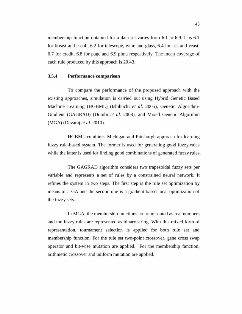
3.5.4 Performance comparison

To compare the performance of the proposed approach with the

existing approaches, simulation is carried out using Hybrid Genetic Based

Machine Learning (HGBML) (Ishibuchi et al. 2005), Genetic Algorithm-

Gradient (GAGRAD) (Dombi et al. 2008), and Mixed Genetic Algorithm

(MGA) (Devaraj et al. 2010).

HGBML combines Michigan and Pittsburgh approach for learning

fuzzy rule-based system. The former is used for generating good fuzzy rules

while the latter is used for finding good combinations of generated fuzzy rules.

The GAGRAD algorithm considers two trapezoidal fuzzy sets per

variable and represents a set of rules by a constrained neural network. It

refines the system in two steps. The first step is the rule set optimization by

means of a GA and the second one is a gradient based local optimization of

the fuzzy sets.

In MGA, the membership functions are represented as real numbers

and the fuzzy rules are represented as binary string. With this mixed form of

representation, tournament selection is applied for both rule set and

membership function. For the rule set two-point crossover, gene cross swap

operator and bit-wise mutation are applied. For the membership function,

arithmetic crossover and uniform mutation are applied.

46

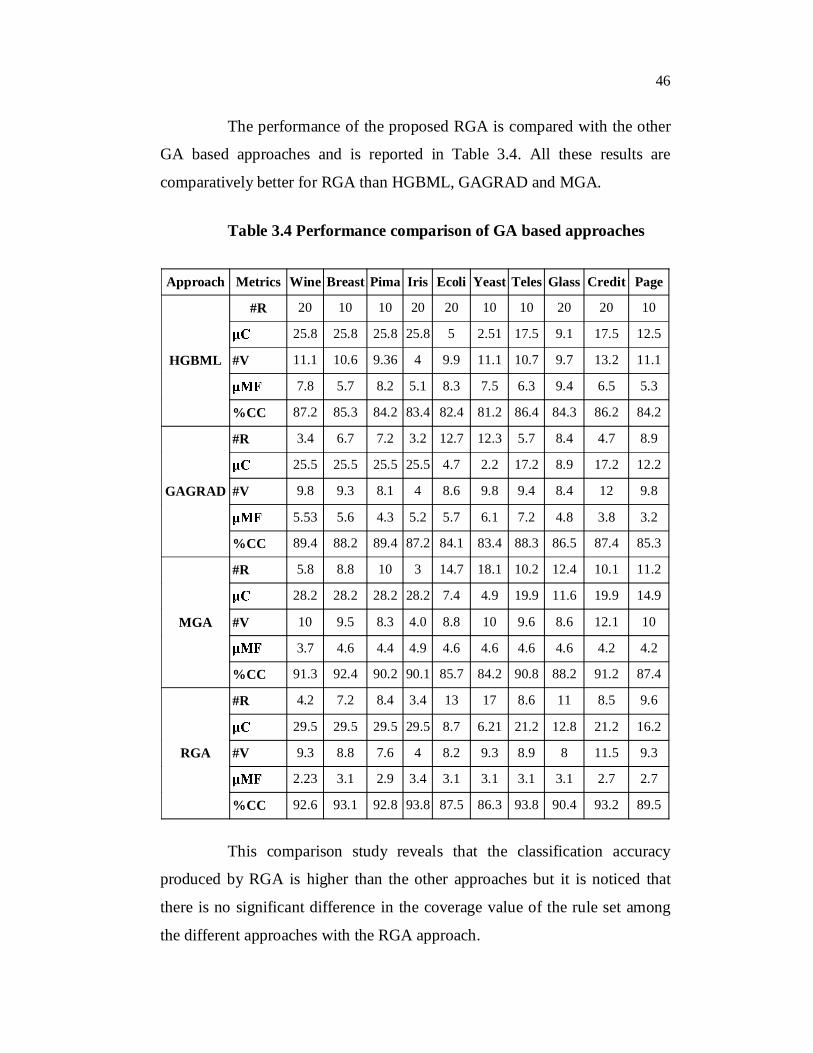
The performance of the proposed RGA is compared with the other

GA based approaches and is reported in Table 3.4. All these results are

comparatively better for RGA than HGBML, GAGRAD and MGA.

Table 3.4 Performance comparison of GA based approaches

Approach Metrics Wine Breast Pima Iris Ecoli Yeast Teles Glass Credit Page

HGBML

#R 20 10 10 20 20 10 10 20 20 10

25.8 25.8 25.8 25.8 5 2.51 17.5 9.1 17.5 12.5

#V 11.1 10.6 9.36 4 9.9 11.1 10.7 9.7 13.2 11.1

7.8 5.7 8.2 5.1 8.3 7.5 6.3 9.4 6.5 5.3

%CC 87.2 85.3 84.2 83.4 82.4 81.2 86.4 84.3 86.2 84.2

GAGRAD

#R 3.4 6.7 7.2 3.2 12.7 12.3 5.7 8.4 4.7 8.9

25.5 25.5 25.5 25.5 4.7 2.2 17.2 8.9 17.2 12.2

#V 9.8 9.3 8.1 4 8.6 9.8 9.4 8.4 12 9.8

5.53 5.6 4.3 5.2 5.7 6.1 7.2 4.8 3.8 3.2

%CC 89.4 88.2 89.4 87.2 84.1 83.4 88.3 86.5 87.4 85.3

MGA

#R 5.8 8.8 10 3 14.7 18.1 10.2 12.4 10.1 11.2

28.2 28.2 28.2 28.2 7.4 4.9 19.9 11.6 19.9 14.9

#V 10 9.5 8.3 4.0 8.8 10 9.6 8.6 12.1 10

3.7 4.6 4.4 4.9 4.6 4.6 4.6 4.6 4.2 4.2

%CC 91.3 92.4 90.2 90.1 85.7 84.2 90.8 88.2 91.2 87.4

RGA

#R 4.2 7.2 8.4 3.4 13 17 8.6 11 8.5 9.6

29.5 29.5 29.5 29.5 8.7 6.21 21.2 12.8 21.2 16.2

#V 9.3 8.8 7.6 4 8.2 9.3 8.9 8 11.5 9.3

2.23 3.1 2.9 3.4 3.1 3.1 3.1 3.1 2.7 2.7

%CC 92.6 93.1 92.8 93.8 87.5 86.3 93.8 90.4 93.2 89.5

This comparison study reveals that the classification accuracy

produced by RGA is higher than the other approaches but it is noticed that

there is no significant difference in the coverage value of the rule set among

the different approaches with the RGA approach.

47

3.6 SUMMARY

The major issue in the development of Fuzzy Classifier is the

formation of fuzzy if-then rules and the membership function. In this chapter

a real coded version of the genetic algorithm is proposed to develop the fuzzy

classifier. The proposed RGA uses advanced and problem specific operators

to improve the convergence and quality of the solution. Simulation result

shows that the proposed RGA works well and produces minimum number of

rules with higher classification accuracy when compared with Simple GA.

Even though the genetic operators used in RGA are central to the

success of its search for optimal membership and rule set formation, they are

computationally expensive and consume more computation time. Further, the

RGA may result in local optima when it is applied for the classification of

complex data.

To overcome this difficulty and to improve the performance of the

fuzzy classifier design, Particle Swarm Optimization (PSO) approach is

presented in the next chapter.