Biomimetics: Learning From Nature for Novel Material Concepts

Novel Control Concepts for HeterogeneousSystems
Michael HertyIGPM, RWTH Aachen University
Workshop IV: Social Dynamics beyond Vehicle Autonomy1st December 2020
1 / 20

Focus on Some Aspects of Social Dynamics beyond VehicleAutonomy at Interface to possible Mathematical Questions
I Heterogeneous traffic andsurroundings conditions arelikely to be impossible todescribe by deterministicmodels
I Different scales are presentin integrated social andtraffic models due to e.g.typical speeds or group sizes
I LV5 autonomy requirespossibly provable stablecontrol mechanisms toguarantee traffic safety
2 / 20

Possible Mathematical Descriptions and QuestionsAspect
I Heterogeneous traffic andsurroundings conditions arelikely to be impossible todescribe by deterministicmodels
I LV5 autonomy requirespossibly provable stablecontrol mechanisms toguarantee traffic safety
I Different scales are presentin integrated social andtraffic models differentiatingbetween typical speeds andgroup sizes
Mathematical terms
I Uncertainty quantificationmethods for different trafficmodels, here: hyperbolicflow models
I Stability / Optimality /Robustness of suitableclosed loop controlstrategies, here: MPC
I Control across scales innonlinear setting, here:optimal control for swarmingtype
Aim is to highlight possible contributions or mathematical methods
3 / 20

(Vehicular)Traffic Modeling at Different Scales due toSpatial, Temporal or Agent AggregationHPRV_BGKmodels_v4.tex 22-12-2018 14:46
Hierarchy of tra�c models
Microscopic scale Mesoscopic scale Macroscopic scale
Spatially homogeneous model (Section 2):
@tf(t, v) = Q[f, f ](t, v)
The solution of Q[f, f ] = 0 provides the
distribution at equilibrium Mf (v; ⇢)
Classical BGK model (Section 3.2):
@tf(t, x, v)+v@xf(t, x, v) =1
✏(Mf (v; ⇢) � f(t, x, v))
Sub-characteristic conditionRV
v2@⇢Mf (v; ⇢)dv ��R
V@⇢Mf (v; ⇢)dv
�2never satisfied in dense tra�c
Payne-Whitham type model (Section 3.2):
@t⇢ + @x⇢u = 0
@t⇢u + @x
Z
V
v2f(t, x, v)dv =
1
✏(Qeq(⇢) � ⇢u)
Sub-characteristic conditionU 0
eq(⇢)2⇢2 < 0
never satisfied
Bando’s model (Section 3.2):
xi = vi
vi =1
✏(Ueq(⇢i) � vi)
It does not consider the interaction term
and it is unstable if ✏ > 12|U0
eq(⇢)|
Follow-the-leader model (Section 4.1):
xi = vi = wi � h(⇢i)
and
vi = C�(vi+1�vi)
(xi+1�xi)�+1 + 1
✏ (Veq(⇢i) � vi)
or
wi = 1✏ (Veq(⇢i) + h(⇢i) � wi)
Modified BGK model (Section 4.2):
@tg(t, x, w)+@x(w�p(⇢))g(t, x, w) =1
✏(Mg(w; ⇢) � g(t, x, w))
The sub-characteristic condition is conditionally
verified in dense tra�c
Aw-Rascle and Zhang model (Section 3.3):
@t⇢ + @x(q � ⇢h(⇢)) = 0
@tq + @x
q2
⇢� qh(⇢)
!=
1
✏(Qeq(⇢) + ⇢h(⇢) � q)
where q = ⇢u + ⇢h(⇢).
Sub-characteristic condition U 0eq � �h0(⇢)
conditionally verified in dense tra�c
Closure Ueq(⇢) =R
Vfdv
and Qeq(⇢) = ⇢Ueq(⇢)Closure Ueq(⇢) =
RV
fdvand Qeq(⇢) = ⇢Ueq(⇢)
Figure 1.1: Schematic summary of the work.
of a BGK-type model for tra�c flow. This approach has also the advantage of prescribing themesoscopic step between the microscopic follow-the-leader model and the macroscopic Aw-Rascleand Zhang model. Finally, we discuss the results and possible perspectives in Section 5.
2 Review of a homogeneous kinetic model
Recent homogeneous kinetic model for tra�c flow have been discussed e.g. in [43, 45]. Themodel proposed therein is used as starting point for the discussion in the following. However, theparticular choice below is not required for the shown results later.
General kinetic tra�c models of the form read
@tf(t, x, v) + v@xf(t, x, v) =1
✏Q[f, f ](t, x, v), (2.1)
wheref(t, x, v) : R+ ⇥ R ⇥ V ! R+ (2.2)
is the mass distribution function of the flow, i.e. f(t, x, v)dxdv gives the number of vehicles in[x, x + dx] with velocity in [v, v + dv] at time t > 0. Moments of the kinetic distribution functionf allow to define the usual macroscopic quantities for tra�c flow
⇢(t, x) =
Z
V
f(t, x, v)dv, (⇢u)(t, x) =
Z
V
vf(t, x, v)dv, u(t, x) =1
⇢
Z
V
vf(t, x, v)dv (2.3)
yielding density, flux and mean speed of vehicles, respectively, at time t and position x. The spaceV := [0, VM ] is the space of microscopic speeds. We suppose that V is limited by a maximumspeed VM > 0, which may depend on several factors, and that the density is also limited by amaximum density ⇢M . Throughout the work we will take dimensionless quantities, thus VM = 1and ⇢M = 1.
In [43] the spatially homogeneous kinetic model corresponding to (2.1) has been discussed:
@tf(t, v) =1
✏Q[f, f ](t, v). (2.4)
3
I Diagram of some examples of traffic modelsI Depending on type of interaction coupling on different levels
possible e.g. individual or fluid4 / 20

Modeling Influence of Heterogeneous Conditions byMethods of Uncertainty Quantification
Exemplify on fluid–like (macroscopic) traffic flow model for densityρ = ρ(t, x), velocity v = v(t, x), property z = z(t, x)
∂t
(ρz
)+ ∂x
(ρvzv
)=
(0
1τ (ρ (Ueq(ρ)− v))
), z = ρv + ρp(ρ)
I Model effect of heterogeneous conditions by random variableξ with given probability distribution P
I Example: relaxation parameter τ = τ0 + ξ or initial orboundary conditions
I Simplest case: Random variable does not have underlyingdynamic: introduces parametric uncertainty also called ξ:ρ = ρ(t, x , ξ) 1
Efficient model predictions E(ρ(t, x)) and Var(ρ(t, x))?1and similar for the functions v , z
5 / 20

Generalized Polynomial Chaos Expansion or Karuhn–LoeveExpansion
Stochastic hyperbolic equation for ρ = ρ(t, x , ξ) with uncertainrelaxation time
∂t
(ρz
)+ ∂x
(ρvzv
)=
(0
1τ(ξ) (ρ (Ueq(ρ)− v))
)
I Multi-Level Monte Carlo, Stochastic Collocation, Momentmethods, . . .
I (Truncated) Series expansion in ξ base functionsφi (ξ), i = 0, . . . orthogonal w.r.t. to weight associate to P
ρ(t, x , ξ) =K∑
i=0
ρi (t, x)φi (ξ)
I E.g. for Legendre polynomials E(ρ(t, x)) = ρ0(t, x) andVar(ρ(t, x)) =
∑i≥1
ρi (t, x)
6 / 20

Mathematical Questions on Well-Posedness
Stochastic hyperbolic equation for ρ = ρ(t, x , ξ) transformed toSystem of transport equations of size 2(K + 1) for coefficients~ρ = (ρ0, . . . , ρK ) :
∂t
(~ρ~z
)+ ∂x
∫F (~ρ, ~z , ~v)~φdP =
∫S(~ρ, ~z , ~v)~φdP
I K = 0 is the deterministic fluid model
I Formulation assumes the solution ρ belongs to the space of2K + 1 base functions in ξ
I Requires to define Galerkin projection of F , i.e. (ρv) possible,requires a priori computation of a tensor
M`,i ,k =
∫φ`(ξ)φi (ξ)φk(ξ)dP
7 / 20

Mathematical Questions on Well-Posedness (cont’d)
Stochastic hyperbolic equation for ρ = ρ(t, x , ξ) transformed tosystem of transport equations of size 2(K + 1) for coefficients
∂t
(~ρ~z
)+ ∂x
∫F (~ρ,~z, ~v)~φdP =
∫S(~ρ,~z, ~v)~φdP
I K = 1 and gPC expansionof (ρ, z , v) leads to loss ofhyperbolicity
I Explicit example availablehaving complex eigenvaluesof the projected flux function
I Local Lax–Friedrichs schemeconverges but yieldsqualitatively wrong solution
0.2 0.4 0.6 0.8 1 1.2 1.4 1.6 1.8 2
0.2
0.3
0.4
0.5
0.6
0.7
Reference solution
ref-sol
0 0.5 1 1.5 20.2
0.3
0.4
0.5
0.6
0.7
0.8Legendre basis and K=2
Mean of ;Mean ' Var
8 / 20

Hyperbolic gPC Formulation
Stochastic hyperbolic equation for ρ = ρ(t, x , ξ) transformed tosystem of transport equations of size 2(K + 1) for coefficients
∂t
(~ρ~z
)+ ∂x
∫F (~ρ,~z, ~v)~φdP =
∫S(~ρ,~z, ~v)~φdP
I Expand only (ρ, z) not vand recompute coefficient inv
I gPC projection ofv = z
ρ − p(ρ) requires tosolve the (linear) system
P(~ρ)~v = ~z − Pγ+1(ρ)
with P(ρ) = ~ρTM.
0.2 0.4 0.6 0.8 1 1.2 1.4 1.6 1.8 2
0.2
0.3
0.4
0.5
0.6
0.7
Reference solution
ref-sol
0 0.2 0.4 0.6 0.8 1 1.2 1.4 1.6 1.8 2
x
0.1
0.2
0.3
0.4
0.5
0.6
0.7
0.8
;
Mean of ;Reference solMean ' Var
9 / 20

Results on the gPC Formulation
I P(ρ) is positive definite for asubclass of base functions
I Hyperbolicity: Expansion in(ρ, z) and projection yields astrictly hyperbolic system forρ0 > 0
I Consistency: fordeterministic τ → 0 recoverthe gPC formulation of thescalar (hyperbolic) LWRmodel
I Numerically: Observeconvergence to reference forK →∞
0 0.2 0.4 0.6 0.8 1 1.2 1.4 1.6 1.8 2
x
0.25
0.3
0.35
0.4
0.45
0.5
0.55
0.6
0.65
0.7
0.75
;
K=1
Mean of ;Reference solMean ' Var
0 0.2 0.4 0.6 0.8 1 1.2 1.4 1.6 1.8 2
x
0.25
0.3
0.35
0.4
0.45
0.5
0.55
0.6
0.65
0.7
0.75
;
K=63
Mean of ;Reference solMean ' Var
Solution to Riemann problem K = 1 and K = 63 modes
10 / 20

Recall Example of Hierarchy of Traffic ModelsHPRV_BGKmodels_v4.tex 22-12-2018 14:46
Hierarchy of tra�c models
Microscopic scale Mesoscopic scale Macroscopic scale
Spatially homogeneous model (Section 2):
@tf(t, v) = Q[f, f ](t, v)
The solution of Q[f, f ] = 0 provides the
distribution at equilibrium Mf (v; ⇢)
Classical BGK model (Section 3.2):
@tf(t, x, v)+v@xf(t, x, v) =1
✏(Mf (v; ⇢) � f(t, x, v))
Sub-characteristic conditionRV
v2@⇢Mf (v; ⇢)dv ��R
V@⇢Mf (v; ⇢)dv
�2never satisfied in dense tra�c
Payne-Whitham type model (Section 3.2):
@t⇢ + @x⇢u = 0
@t⇢u + @x
Z
V
v2f(t, x, v)dv =
1
✏(Qeq(⇢) � ⇢u)
Sub-characteristic conditionU 0
eq(⇢)2⇢2 < 0
never satisfied
Bando’s model (Section 3.2):
xi = vi
vi =1
✏(Ueq(⇢i) � vi)
It does not consider the interaction term
and it is unstable if ✏ > 12|U0
eq(⇢)|
Follow-the-leader model (Section 4.1):
xi = vi = wi � h(⇢i)
and
vi = C�(vi+1�vi)
(xi+1�xi)�+1 + 1
✏ (Veq(⇢i) � vi)
or
wi = 1✏ (Veq(⇢i) + h(⇢i) � wi)
Modified BGK model (Section 4.2):
@tg(t, x, w)+@x(w�p(⇢))g(t, x, w) =1
✏(Mg(w; ⇢) � g(t, x, w))
The sub-characteristic condition is conditionally
verified in dense tra�c
Aw-Rascle and Zhang model (Section 3.3):
@t⇢ + @x(q � ⇢h(⇢)) = 0
@tq + @x
q2
⇢� qh(⇢)
!=
1
✏(Qeq(⇢) + ⇢h(⇢) � q)
where q = ⇢u + ⇢h(⇢).
Sub-characteristic condition U 0eq � �h0(⇢)
conditionally verified in dense tra�c
Closure Ueq(⇢) =R
Vfdv
and Qeq(⇢) = ⇢Ueq(⇢)Closure Ueq(⇢) =
RV
fdvand Qeq(⇢) = ⇢Ueq(⇢)
Figure 1.1: Schematic summary of the work.
of a BGK-type model for tra�c flow. This approach has also the advantage of prescribing themesoscopic step between the microscopic follow-the-leader model and the macroscopic Aw-Rascleand Zhang model. Finally, we discuss the results and possible perspectives in Section 5.
2 Review of a homogeneous kinetic model
Recent homogeneous kinetic model for tra�c flow have been discussed e.g. in [43, 45]. Themodel proposed therein is used as starting point for the discussion in the following. However, theparticular choice below is not required for the shown results later.
General kinetic tra�c models of the form read
@tf(t, x, v) + v@xf(t, x, v) =1
✏Q[f, f ](t, x, v), (2.1)
wheref(t, x, v) : R+ ⇥ R ⇥ V ! R+ (2.2)
is the mass distribution function of the flow, i.e. f(t, x, v)dxdv gives the number of vehicles in[x, x + dx] with velocity in [v, v + dv] at time t > 0. Moments of the kinetic distribution functionf allow to define the usual macroscopic quantities for tra�c flow
⇢(t, x) =
Z
V
f(t, x, v)dv, (⇢u)(t, x) =
Z
V
vf(t, x, v)dv, u(t, x) =1
⇢
Z
V
vf(t, x, v)dv (2.3)
yielding density, flux and mean speed of vehicles, respectively, at time t and position x. The spaceV := [0, VM ] is the space of microscopic speeds. We suppose that V is limited by a maximumspeed VM > 0, which may depend on several factors, and that the density is also limited by amaximum density ⇢M . Throughout the work we will take dimensionless quantities, thus VM = 1and ⇢M = 1.
In [43] the spatially homogeneous kinetic model corresponding to (2.1) has been discussed:
@tf(t, v) =1
✏Q[f, f ](t, v). (2.4)
3
I Results on Uncertainty Quantification on Mesoscopic LevelExist
I Open or closed loop control consistent across the scales
11 / 20

Optimal Control Across Scales in Nonlinear DynamicsWhere may this problem arise?
I Control strategies for N(interacting) agents likelarge crowds of people,suitably many vehicles onlarge–scale highway system
I Goal is a consistent controlfor any number of agentsincluding N =∞
I Exemplified on the case oftypical swarming typeinteractions with state xwith single control u
uncontrolled and controlled on particle and meanfield
d
dtxi =
1
N
N∑
j=1
p(xi , xj , u), u = argmin u
∫ T
0
1
N
N∑
j=1
φ(xj , u)dt
12 / 20

Finite (P) and corresponding Infinite (MF) OptimalControl Problem
(P) u = argmin u
∫ T
0
1
N
∑
j
φ(xi , u)dt s.t.d
dtxi =
1
N
∑
j
p(xi , xj , u)
(MF ) u = argminu
∫ T
0
∫φ(x , u)µ(x , t)dx s.t. 0 = ∂tµ+ divx (µGµ)
ODE
I Pontryagins MaximumPrinciple and adjointvariables zi ∈ RK
I BBGKY hierarchy leads tojoint meanfield distributiong = g(t, x , z) in state x andadjoint z for N =∞
MFI L2−first–order optimality
conditions
0 = ∂tµ + divx(µGµ
),
0 = −∂tλ−∇xλTGµ−
−∫µ(y, t)∇xλ(y, t)T p(y, x, u)dy + φ
Necessary conditions for consistent control?13 / 20
Necessary Conditions for Consistent Controls (P) vs (MF)
Lemma. Decompose g(t, x , z) = µ(x , t)µc(z , x , t). Then, thefinite and infinite problem are consistent provided that
∇xλ(t, x) =
∫zµc(z , x , t)dz
I Multiplier λ in the L2 sense is gradientof the expectation of conditionalprobability density of BBGKYhierarchy
I Mesoscopic formulation allows toanalyse consistent numericaldiscretization
I Extension to Game Theoretic Settingpossible, e.g. Stackelberg game withinfinitely many players
14 / 20

Including Uncertainty Using MPC Framework
I Open loop controlmaybe notsuitable foron-board/onlinecontrol of LV5 cars
I Sudden,unexpected eventsneed to beaccounted for bysuitable controlmeasures
I Receding horizonorModel–PredictiveControl
✓1
✓2✓3
✓ = 0
✓ = ⇡/2
✓ /2 [�⇡/2, ⇡/2]
✓ /2 [�⇡/2, ⇡/2]
vi sin (✓1) < 0
vi sin�✓k
�> 0, k = 2, 3
y
x
i
2
3
1
Figure 3: Choice of the interacting car in the case vi > 0. The interacting vehicle will be car 2,namely the nearest vehicle in the driving direction of vehicle i.
two-dimensional case (see (7)), respectively. Observe that
⇢2Di ! ⇢1D
i , as �Y,��yj(i) � yi
��! 0+
only if we assume that
lim�Y !0+
(yj(i)�yi)!0+
�Y��yj(i) � yi
�� = 1. (8)
The interacting vehicle j(i) is determined by the following map
i 7! j(i) = arg minh=1,...,N
vi sin ✓h>0
✓h2[�⇡2 ,⇡2 ]
kQh � Qik2 . (9)
This choice is motivated as follows, see also Figure 3. Assume that each test vehicle i defines acoordinate system in which the origin is its right rear corner if vi � 0 and its left rear corner ifvi < 0. We are indeed dividing the road in four areas. Let ✓h be the angle between the x-axis (inthe car coordinate system) and the position vector Qh of vehicle h. Then the request ✓h 2
⇥�⇡
2 , ⇡2
⇤
allows to consider only cars being in front of vehicle i. Instead, the request vi sin ✓h > 0 allowsto consider only cars in the driving direction of vehicle i. Among all these vehicles we choose thenearest one. Therefore, (9) can be rewritten as
i 7! j(i) = arg minh=1,...,N
vi(yh�yi)>0xh>xi
kQh � Qik2 .
6
15 / 20
Performance of Receding Horizon Control Depending onPrediction Horizon
Evolution of state dynamics under receding horizon control withdifferent prediction horizons N on Meanfield
16 / 20

Analytical Performance Bounds Available
V∗(τ, Y ) = minu
∫ T
τh(X ) +
ν
2u2ds, x′i (t) = f (xi (t), X−i (t)) + u
VMPC (τ, y) =
∫ T
τh(XMPC ) +
ν
2(uMPC )2ds, (xMPC
i )′(t) = f (XMPC (t)) + uMPC
I V ∗ value function for (full) optimal control u and initial dataX (τ) = Y
I VMPC receding horizon control dynamics and correspondingvalue function
I Grune [2009]: Finitely many particles. There exists 0 < α < 1such that
VMPC (τ, y) ≤ 1
αV ∗(τ, y)
I α depends on size of horizon and growth conditions of f
17 / 20
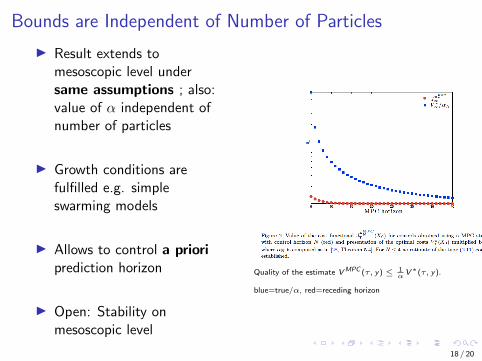
Bounds are Independent of Number of Particles
I Result extends tomesoscopic level undersame assumptions ; also:value of α independent ofnumber of particles
I Growth conditions arefulfilled e.g. simpleswarming models
I Allows to control a prioriprediction horizon
I Open: Stability onmesoscopic level
Quality of the estimate VMPC (τ, y) ≤ 1αV∗(τ, y).
blue=true/α, red=receding horizon
18 / 20

Summary
I Modeling heterogeneous aspects by random variables leads tointeresting mathematical questions for example onmacroscopic level
I Similar question of uncertainty on kinetic scale have beeninvestigated but links are not fully explored
I For control actions some links between microscopic andkinetic scale are established
I Receding horizon methods for treating time dependentuncertainty are also scale invariant
Present results here are in collaboration with S. Gerster, E.Iacomini, C. Ringhofer and M. Zanella.
19 / 20


![Heterogeneous Catalysis [Basic Concepts] - Jens Norskov](https://static.fdocuments.in/doc/165x107/542ac2c4219acd89798b472d/heterogeneous-catalysis-basic-concepts-jens-norskov.jpg)