Notes on Analytical Mechanics - 3dhouse.se3dhouse.se/ingemar/anmek.pdf · This is done by means of...
143
Notes on Analytical Mechanics Ingemar Bengtsson (2018)
Transcript of Notes on Analytical Mechanics - 3dhouse.se3dhouse.se/ingemar/anmek.pdf · This is done by means of...

Notes on Analytical Mechanics
Ingemar Bengtsson (2018)


Contents
1 The Best of all Possible Worlds page 1
1.1 Analytical and Hamiltonian mechanics . . . . . . . . . . . . . 21.2 The calculus of variations . . . . . . . . . . . . . . . . . . . . . 61.3 How to solve equations . . . . . . . . . . . . . . . . . . . . . . 81.4 Phase space . . . . . . . . . . . . . . . . . . . . . . . . . . . . . 12
2 Lagrangian mechanics 19
2.1 The scope of Lagrangian mechanics . . . . . . . . . . . . . . . 192.2 Constrained systems . . . . . . . . . . . . . . . . . . . . . . . . 222.3 Symmetries . . . . . . . . . . . . . . . . . . . . . . . . . . . . . 26
3 Interlude: Conic sections 33
4 The central force two-body problem 38
4.1 The problem and its formal solution . . . . . . . . . . . . . . . 394.2 Existence and stability of circular orbits . . . . . . . . . . . . . 414.3 Kepler’s First Law . . . . . . . . . . . . . . . . . . . . . . . . . 434.4 Kepler’s Third Law . . . . . . . . . . . . . . . . . . . . . . . . 454.5 Self-similarity and the virial theorem . . . . . . . . . . . . . . 464.6 The three-body problem . . . . . . . . . . . . . . . . . . . . . . 49
5 Small oscillations 54
5.1 Forced oscillations . . . . . . . . . . . . . . . . . . . . . . . . . 545.2 Damped and forced oscillations . . . . . . . . . . . . . . . . . . 575.3 Several degrees of freedom . . . . . . . . . . . . . . . . . . . . 60
6 Rotation and rigid bodies 65
6.1 Rotations . . . . . . . . . . . . . . . . . . . . . . . . . . . . . . 656.2 Rotating coordinate systems . . . . . . . . . . . . . . . . . . . 706.3 The inertia tensor . . . . . . . . . . . . . . . . . . . . . . . . . 736.4 Euler’s equations . . . . . . . . . . . . . . . . . . . . . . . . . . 776.5 The Lagrangian description . . . . . . . . . . . . . . . . . . . . 816.6 The tippe top . . . . . . . . . . . . . . . . . . . . . . . . . . . 85
7 Interlude: Legendre transformations 89

ii Contents
8 The Hamiltonian formulation 93
8.1 Hamilton’s equations and Hamiltonian flows . . . . . . . . . . 938.2 The algebraic structure of mechanics . . . . . . . . . . . . . . . 968.3 Canonical transformations . . . . . . . . . . . . . . . . . . . . 998.4 General transformation theory . . . . . . . . . . . . . . . . . . 1018.5 Kets and bras and all that . . . . . . . . . . . . . . . . . . . . 1048.6 The symplectic form . . . . . . . . . . . . . . . . . . . . . . . . 1088.7 The symplectic one-form . . . . . . . . . . . . . . . . . . . . . 1118.8 The sphere as a phase space . . . . . . . . . . . . . . . . . . . 114
9 Hamilton-Jacobi theory 118
9.1 Geometrical optics . . . . . . . . . . . . . . . . . . . . . . . . . 1189.2 Hamilton’s Principal Function . . . . . . . . . . . . . . . . . . 1219.3 Soluble examples . . . . . . . . . . . . . . . . . . . . . . . . . . 123
10 Integrable and chaotic motion 126
10.1 Can chaos occur? . . . . . . . . . . . . . . . . . . . . . . . . . 12610.2 Integrable systems . . . . . . . . . . . . . . . . . . . . . . . . . 12810.3 Canonical perturbation theory . . . . . . . . . . . . . . . . . . 13110.4 Stability of the Solar System . . . . . . . . . . . . . . . . . . . 134
Appendix 1 Books 137
Index 139

1 The Best of all Possible Worlds
Mechanics is the paradise of the mathematical
sciences, because with it one comes to the fruits
of mathematics
Leonardo da Vinci
Sir Isaac Newton was a Master of the Mint. He also formulated three cele-brated laws of mechanics, which we can paraphrase as follows:
1. A particle not subject to any force moves on a straight line at constantspeed.
2. In the presence of a force, the position of a particle obeys the equations ofmotion
mxi = Fi(x, x) . (1.1)
3. The force exerted by a particle on another is equal in magnitude, but op-posite in direction, to the force exerted by the other particle on the first.
A “particle” is here thought of as an entity characterized by its mass m, itslocation in space, and by nothing else.1 The aim of Newton’s mechanics is topredict the location at arbitrary times, given the position and velocity at someinitial time. This is done by means of a solution of the differential equationsabove.
An overdot denotes differentiation with respect to the time parameter t(this notation, as well as Differential Calculus itself, was invented by Newton),and xi may denote a vector in three-dimensional space. Sometimes it will beunderstood that we are dealing with a set of N particles, and moreover weoften “suppress indices”. Then the force Fi(x, x) is a 3N component functionof the 3N variables xi and their 3N derivatives xi. Since the index notationmay be a bit unfamiliar, let me note that whenever indices occur in a formula,it is understood that they can take any of a specified set of integer values.
1 For further discussion see A. Jenkins, On the title of Moriarty’s ’Dynamics of an Asteroid’,eprint arXiv:1302.5855.

2 The Best of all Possible Worlds
If i ∈ 1, 2, ..., n then eq. (1.1) stands for n separate equations. Throughoutwe employ Einstein’s summation convention, which means that whenever acertain index occurs twice in a particular term, a sum over all its allowedvalues is understood, eg.
xiyi ≡n∑
i=1
xiyi =
n∑
j=1
xjyj = xjyj . (1.2)
It does not matter which letter is being used for a repeated index. To avoidconfusion, the same index never occurs thrice or more in a single term. Insection 8.5 we will introduce index notation in a more sophisticated “tensorial”way, but for the time being this is all there is to it. By the way index notationis not always the best choice—it does not, for instance, make use of any specialproperties of three dimensional space—but it has the advantage that it can beused for everything, which is why I always use it.
1.1 Analytical and Hamiltonian mechanics
What are we to think of Newton’s laws? A physicist might follow Newton inusing them to predict the position of the planets as they go around the sun, andwill conclude that they are very meaningful. A mathematician might say thatthey do not say very much, only that the position of a particle is described by aset of ordinary differential equations. A philosopher might object that they saynothing at all—the first and second law together seem to state that a particlemoves in a straight line, unless it does something else, in which case we say thatit is subject to a force. But the philosopher Kant valued Newton’s laws highly,and tried to prove that they are somehow necessary consequences of the wayour minds perceive the world, and have a status similar to Euclid’s axioms ingeometry. Kant overestimated Newton’s laws, but they do have content as theystand. It is a highly non-trivial fact that a second order differential equationis being postulated, since this means that the position and the velocity can bechosen arbitrarily at a given instant, but not the acceleration. Moreover, theuse of differential equations guarantees that both the past and the future areuniquely determined by the initial values of position and velocity.
Analytical mechanics is at once more general and more special than New-ton’s theory. It is more general because it is more abstract. Its equations donot necessarily describe the positions of particles, but may be applied to muchmore general physical systems (such as field theories, including Einstein’s gen-eral relativity theory). In the version we will study it is more special becauseonly a restricted set of forces will be allowed in eq. (1.1). Let us see what kindof restrictions on the function Fi that are of physical interest. Newton’s thirdlaw is already a restriction. It can be reformulated as the statement that thetotal momentum of a system composed of several particles is conserved:

1.1 Analytical and Hamiltonian mechanics 3
dPidt
≡ d
dt
∑
particles
mxi = 0 , (1.3)
where the sum is over all the particles in the system. The existence of sucha conserved vector is clearly an interesting fact. By the way this formulationis quite superior when we deal with time dependent masses, say with rockets(see exercise 3). Now consider the function
E = T + V =mx2
2+ V (x) , (1.4)
where V is some function of x, known as the potential energy. The function Tis called the kinetic energy, while E itself is the energy of the system. Clearly
E = xi (mxi + ∂iV (x)) . (1.5)
It follows that if the force is given by
Fi(x, x) = Fi(x) = −∂iV (x) , (1.6)
then the energy of the system is conserved. Systems for which a conservedenergy function exists are called conservative. In our example, and indeed inmany interesting cases, the energy can be divided into kinetic and potentialparts, and the equation of motion is given by
mxi = −∂iV (x) . (1.7)
This move is typical of analytical mechanics, where vectors are usually derivedfrom scalar functions.
Analytical mechanics devises methods to derive the differential equations de-scribing a given system, strategies for solving them, and ways of describingthe solutions if they cannot be obtained in explicit form.2
We will tentatively restrict ourselves to conservative systems only. If you likethis is a strengthening of the third law, and it is believed that all isolatedsystems in Nature are of this type.
What we are trying to do is to find some properties that all the Laws ofPhysics, and in particular all allowed equations of motion, have in common.Now the philosopher Leibniz—who was the other of the two inventors of Dif-ferential Calculus—argued that we live in the best of all possible worlds. Is itevident from eq. (1.7) that this is so? Indeed it is, as was realized half a cen-tury after the publication of Newton’s Principia. The inspiration came fromoptics, and the laws of reflection and refraction. It was known that the angle
2 As a definition, this is a little vague. Mechanique Analitique was the title of a book written byLagrange—“the beauty of the method so suiting the dignity of the results, as to make of his greatwork a kind of scientific poem”, to quote Hamilton.

4 The Best of all Possible Worlds
of reflection is equal to the angle of incidence, and it was observed by theGreeks that this implies that light always travels on the shortest path avail-able between two points A and B, subject to the restriction that it should bereflected against the surface. If the angle of reflection were to differ from theangle of incidence, the distance covered by light in going from A to B wouldbe greater than it has to be. For refraction, we have Snell’s Law. Any mediumcan be assigned an index of refraction n, and the angle of refraction is relatedto the angle of incidence through
n1 sin θi = n2 sin θr . (1.8)
Fermat noted that if
n =c
v, (1.9)
where v is the velocity of light in the medium and c is a constant (independentof the medium), then Snell’s law can be derived from what is now known asFermat’s principle, namely that the time taken for light to go from A to B is aminimum. Fermat’s principle unifies the laws of refraction and reflection, sinceit also implies the equality between the angles of incidence and reflection.
More generally the index of refraction may be a function n(x) of position,say through a dependence on temperature. This is what causes mirages. Tostudy this mathematically we imagine that we evaluate the curve integral
I = c
∫
γ
dt =
∫
γ
cds
v=
∫
γ
n(x(s))ds (1.10)
along an arbitrary path γ(s) between A and B. Then the path actually takenby light in going from A to B through the medium is that specific path whichresults in the smallest possible value of the integral I. This path may well notbe a straight line. The question is how to do the optimization. We will sooncome to it.
Is there a similar principle underlying mechanics? Maupertius realized that,at least for systems obeying eq. (1.7), there is.3 Consider two points A and B,and suppose that a particle starts out at A at time t = t1, and then moves alongan arbitrary path from A to B with whatever speed that is consistent withthe requirement that it should arrive at B at the time t = t2. In mathematicalterms we are dealing with a function x(t) such that
x(t1) = xA x(t2) = xB , (1.11)
but otherwise arbitrary. For any such function x(t) we can evaluate the integral
3 It was claimed that Leibniz knew the result before him, but in the resulting priority fight Mau-perties was strongly supported by Euler. Historians have since found out that the result was, infact, first arrived at in an unpublished investigation by Euler—who, unlike some scientists onecould mention, never cared strongly about priority as far as he himself was concerned.

1.1 Analytical and Hamiltonian mechanics 5
S[x(t)] =
∫ t2
t1
dt (T − V ) =
∫ t2
t1
dt
(
mx2
2− V (x)
)
. (1.12)
S is known as the action. It is a functional, i.e. a function of a function—thefunctional S[x(t)] assigns a real number to any function x(t). Note that S[x(t)]is not a function of t, hence the square bracket notation. On the other handit is a function of xA, xB, t1, and t2, but this is rarely written out explicitly.
The statement, to be verified in the next section, is that the action func-tional (1.12) has an extremum (not necessarily a minimum) for precisely thatfunction x(t) which obeys the differential equation (1.7). This is known asHamilton’s Principle, or—with less than perfect historical and mathematicalaccuracy—as the Principle of Least Action.
Hamiltonian mechanics deals with those, and only those, equations of motionwhich can be derived from Hamilton’s Principle, for some choice of the actionfunctional.
This is a much more general class than that given by eq. (1.7), but it doesexclude some cases of physical interest. Hamiltonian mechanics forms only apart of analytical mechanics—namely that part that we will focus on.
Note once again what is going on. The original task of mechanics was topredict the trajectory of a particle, given a small set of data concerning itsstate at some intial time t. We claim that there exists another formulation ofthe problem, where we can deduce the trajectory given half as much data ateach of two different times. So there seems to be a local, causal way of lookingat things, and an at first sight quite different global, teleological viewpoint.The claim begins to look reasonable when we observe that the amount of “freedata” in the two formulations are the same. Moreover, if the two times t1and t2 approach each other infinitesimally closely, then what we are in effectspecifying is the position and the velocity at time t1, just as in the causalapproach.
Why do principles like Fermat’s and Hamilton’s work? In both cases, we areextremizing a quantity evaluated along a path, and the path actually takenby matter in nature is the one which makes the quantity in question assumean extremal value. The point about extrema—not only minima—is that if thepath is varied slightly away from the extremal path, to a path which differs toorder ǫ from the extremal one, then the value of the path dependent quantitysuffers a change which is of order ǫ squared. At an extremum the first derivativevanishes. In the case of optics, we know that the description of light as a bundleof rays is valid only in the approximation where the wavelength of light ismuch less than the distance between A and B. In the wave theory, in a way,every path between A and B is allowed. If we vary the path slightly, the timetaken by light to arrive from A to B changes, and this means that it arrivesout of phase with the light arriving along the first path. If the wavelengthis very small, phases from light arriving by different paths will be randomly
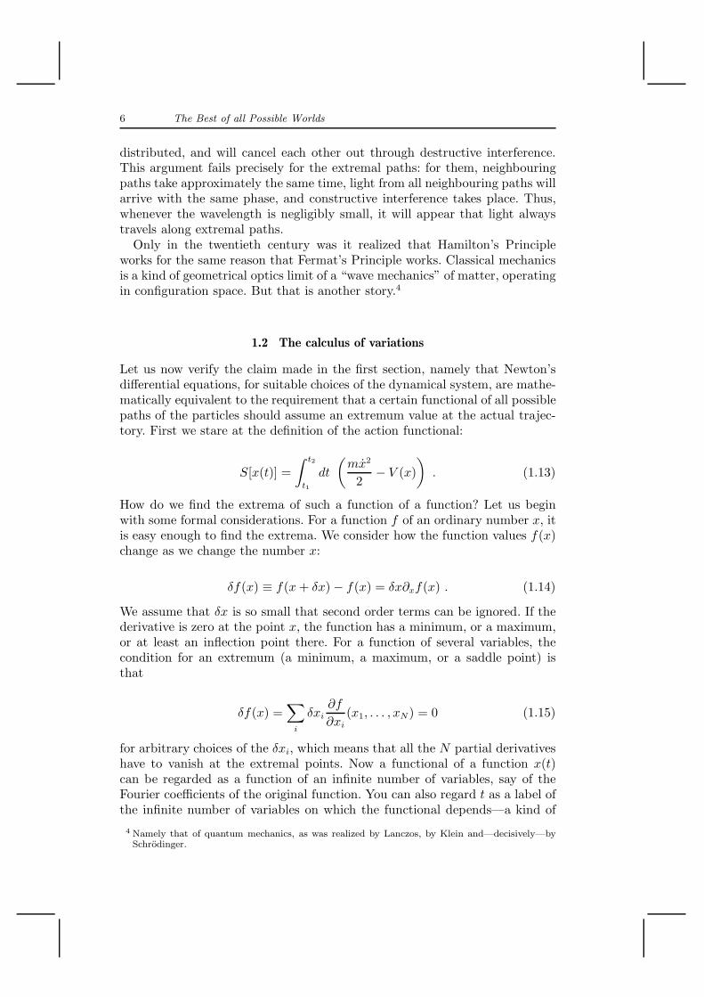
6 The Best of all Possible Worlds
distributed, and will cancel each other out through destructive interference.This argument fails precisely for the extremal paths: for them, neighbouringpaths take approximately the same time, light from all neighbouring paths willarrive with the same phase, and constructive interference takes place. Thus,whenever the wavelength is negligibly small, it will appear that light alwaystravels along extremal paths.
Only in the twentieth century was it realized that Hamilton’s Principleworks for the same reason that Fermat’s Principle works. Classical mechanicsis a kind of geometrical optics limit of a “wave mechanics” of matter, operatingin configuration space. But that is another story.4
1.2 The calculus of variations
Let us now verify the claim made in the first section, namely that Newton’sdifferential equations, for suitable choices of the dynamical system, are mathe-matically equivalent to the requirement that a certain functional of all possiblepaths of the particles should assume an extremum value at the actual trajec-tory. First we stare at the definition of the action functional:
S[x(t)] =
∫ t2
t1
dt
(
mx2
2− V (x)
)
. (1.13)
How do we find the extrema of such a function of a function? Let us beginwith some formal considerations. For a function f of an ordinary number x, itis easy enough to find the extrema. We consider how the function values f(x)change as we change the number x:
δf(x) ≡ f(x+ δx) − f(x) = δx∂xf(x) . (1.14)
We assume that δx is so small that second order terms can be ignored. If thederivative is zero at the point x, the function has a minimum, or a maximum,or at least an inflection point there. For a function of several variables, thecondition for an extremum (a minimum, a maximum, or a saddle point) isthat
δf(x) =∑
i
δxi∂f
∂xi(x1, . . . , xN) = 0 (1.15)
for arbitrary choices of the δxi, which means that all the N partial derivativeshave to vanish at the extremal points. Now a functional of a function x(t)can be regarded as a function of an infinite number of variables, say of theFourier coefficients of the original function. You can also regard t as a label ofthe infinite number of variables on which the functional depends—a kind of
4 Namely that of quantum mechanics, as was realized by Lanczos, by Klein and—decisively—bySchrodinger.
1.2 The calculus of variations 7
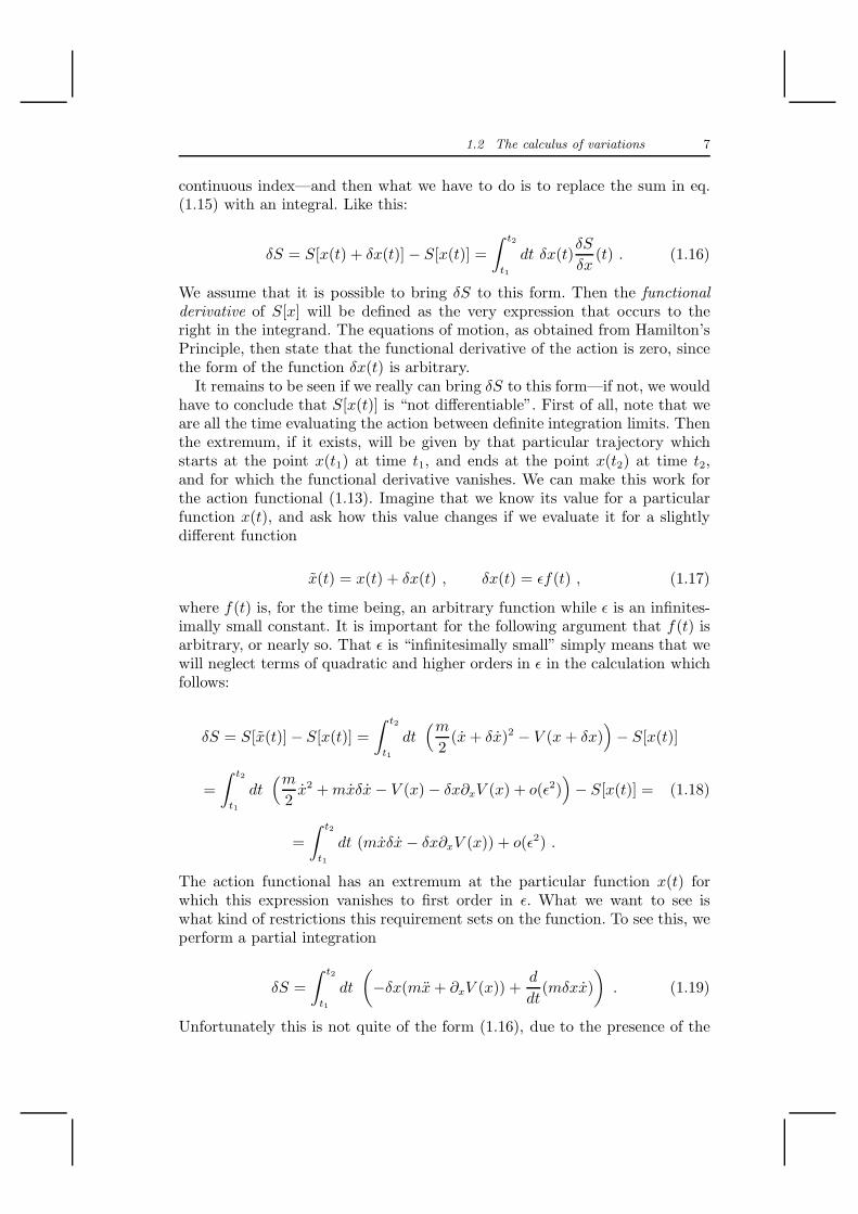
continuous index—and then what we have to do is to replace the sum in eq.(1.15) with an integral. Like this:
δS = S[x(t) + δx(t)] − S[x(t)] =
∫ t2
t1
dt δx(t)δS
δx(t) . (1.16)
We assume that it is possible to bring δS to this form. Then the functional
derivative of S[x] will be defined as the very expression that occurs to theright in the integrand. The equations of motion, as obtained from Hamilton’sPrinciple, then state that the functional derivative of the action is zero, sincethe form of the function δx(t) is arbitrary.
It remains to be seen if we really can bring δS to this form—if not, we wouldhave to conclude that S[x(t)] is “not differentiable”. First of all, note that weare all the time evaluating the action between definite integration limits. Thenthe extremum, if it exists, will be given by that particular trajectory whichstarts at the point x(t1) at time t1, and ends at the point x(t2) at time t2,and for which the functional derivative vanishes. We can make this work forthe action functional (1.13). Imagine that we know its value for a particularfunction x(t), and ask how this value changes if we evaluate it for a slightlydifferent function
x(t) = x(t) + δx(t) , δx(t) = ǫf(t) , (1.17)
where f(t) is, for the time being, an arbitrary function while ǫ is an infinites-imally small constant. It is important for the following argument that f(t) isarbitrary, or nearly so. That ǫ is “infinitesimally small” simply means that wewill neglect terms of quadratic and higher orders in ǫ in the calculation whichfollows:
δS = S[x(t)] − S[x(t)] =
∫ t2
t1
dt(m
2(x+ δx)2 − V (x+ δx)
)
− S[x(t)]
=
∫ t2
t1
dt(m
2x2 +mxδx− V (x) − δx∂xV (x) + o(ǫ2)
)
− S[x(t)] = (1.18)
=
∫ t2
t1
dt (mxδx− δx∂xV (x)) + o(ǫ2) .
The action functional has an extremum at the particular function x(t) forwhich this expression vanishes to first order in ǫ. What we want to see iswhat kind of restrictions this requirement sets on the function. To see this, weperform a partial integration
δS =
∫ t2
t1
dt
(
−δx(mx+ ∂xV (x)) +d
dt(mδxx)
)
. (1.19)
Unfortunately this is not quite of the form (1.16), due to the presence of the

8 The Best of all Possible Worlds
total derivative in the integrand. Therefore we impose a restriction on the sofar arbitrary function f(t) that went into the definition of δx, so that
δx(t1) = δx(t2) = 0 . (1.20)
This is a way of saying that we are interested only in functions x(t) thathave certain preassigned starting and end points at specified times. With thisrestriction, the total derivative in eq. (1.19) goes away. The first term hasto vanish for all allowed choices of the functions δx(t). After a moment’sreflection, we see that this can happen only if the factor multiplying δx inthe integrand is zero! Hence we have proved that the action functional has anextremum, among all possible functions obeying
x(t1) = xA x(t2) = xB , (1.21)
for those and only those functions which obey
mx = −∂xV (x) (1.22)
at all intermediate points.So we have proved, in this particular case at least, that Newton’s equations
of motion can be derived from the condition that a certain action functionalshall have an extremum value. Note also that the restrictions that we had toset on the function x(t), eqs. (1.21), make perfect sense. To obtain a definitetrajectory it is not enough to impose the equations of motion. It is also nec-essary to set initial conditions. For differential equations of second order, itis natural to make a choice of x(0) and x(0). From the point of view of theaction, it is natural to impose the value of x(t) at two different times, whichis the same amount of information. It should be noted though that whatevervalues of x(0) and x(0) we choose there is always a unique solution for somerange of t, while it is perfectly possible that the equation of motion is suchthat there is no solution, or several solutions, for a given pair of x(t1) andx(t2).
The rest of this course is an elaboration of the contents of this section. Ifyou have not understood everything perfectly yet there is still time!
1.3 How to solve equations
It is one thing to be able to set up equations for a physical system, and perhapsto prove theorems to the effect that a solution always exists and is unique,given suitable initial conditions. Another issue of obvious interest is how tosolve these equations, or at least how to extract information from them. Whatprecisely do we mean when we say that a differential equation is “soluble”?Consider, as an exercise, a first order differential equation for a single variable:

1.3 How to solve equations 9
x = f(x) , (1.23)
where f is some function. This can be solved by means of separation of vari-ables:
dt =dx
f(x)⇒ t(x) =
∫ x
c
dx′
f(x′), (1.24)
where c is a constant determined by the initial condition. If we do this integral,and then invert the resulting function t(x) to obtain the function x(t), wehave solved the equation. We will regard eq. (1.24) as an implicit definitionof x(t), and eq. (1.23) is soluble in this sense. This is reasonable, since themanipulations required to extract t(x) can be easily done on a computer, to anydesired accuracy, even if we cannot express the integral in terms of elementaryfunctions. But there are some limitations here: It may not be possible to invertthe function t(x) except for small times.
Next consider a second order equation, such as the equation of motion fora harmonic oscillator:
mx = −ax . (1.25)
This is a linear equation, and we know how to express the solution in terms oftrigonometric functions, but our third example—a pendulum of length l—isalready somewhat worse:
ml2θ = −gml sin θ . (1.26)
Let us therefore approach eq. (1.25) in a systematic fashion, which mightyield results also for the pendulum. As a first step, note that any second orderdifferential equation can be rewritten as a pair of coupled first order equations:
p = −ax mx = p . (1.27)
The second equation defines the new variable p. Unfortunately coupled firstorder equations are difficult to solve, except in the linear case when they canbe decoupled through a Fourier transformation.
The number of degrees of freedom of a dynamical system is defined to be onehalf times the number of first order differential equations needed to describethe evolution.
It will turn out that, for systems whose equations of motion are derivablefrom the action principle, the number of first order equations will always beeven, so the number of degrees of freedom is always an integer for such systems.A system with n degrees of freedom will be described by a set of 2n in generalcoupled first order equations, and the difficulties one encounters in trying tosolve them will rapidly become severe.
In the cases at hand, with one degree of freedom only, one uses the fact that

10 The Best of all Possible Worlds
these are conservative systems, which will enable us to reduce the problem tothat of solving a single first order equation. For the harmonic oscillator theconserved quantity is
E =mx2
2+ax2
2. (1.28)
The number E does not depend on t. Equivalently
x2 =2E
m− a
mx2 . (1.29)
Taking a square root we are back to the situation we know, and we proceedas before:
dt = dx
√
m
2E − ax2⇔ t(x) =
∫ x
c
dx′
√
m
2E − ax′2. (1.30)
Inverting the function defined by the integral, we find the solution x(t). Theanswer is a trigonometric function, with two arbitrary constants E and c de-termining its phase and its amplitude. For our purposes the trigonometricfunction is defined by this procedure!
We can play the same trick with the non-linear equation for the pendulum,and we end up with
t(θ) =
∫ θ
c
dθ′√
2ml2
(E + gml cos θ′). (1.31)
We integrate, and we invert. This defines the function θ(t). We could leave itat that, but since our example is a famous one, we manipulate the integral abit further for the fun of it. Make the substitution
sinθ′
2≡ k sinφ′ ⇒ dθ′ =
2k cosφ′ dφ′
√
1 − k2 sin2 φ′. (1.32)
The constant k is undetermined at this stage. The integral becomes
t(θ) =
√
l
2g
∫ φ(θ)
c
2k cosφ′dφ′
√
1 − k2 sin2 φ′
√
Egml
+ 1 − 2 sin2 θ′
2
. (1.33)
The integrand simplifies if we choose the constant k such that
2k2 ≡ E
gml+ 1 . (1.34)
One further substitution takes us to our desired standard form;

1.3 How to solve equations 11
t(θ) =
√
l
g
∫ φ(θ)
c
dφ′
√
1 − k2 sin2 φ′=
/
sinφ′ ≡ x′/
=
√
l
g
∫ x(θ)
c
dx′
√
(1 − x′2)(1 − k2x′2). (1.35)
Just as eq. (1.30) can be taken as an implicit definition of a trigonometricfunction, this integral implicitly defines the function θ(t) as an elliptic function.If you compare it with the previous integral (1.30), you see that an ellipticfunction is a fairly natural generalization of a trigonometric, i.e. “circular”,function. Since elliptic functions turn up in many contexts they have beenstudied in depth by mathematicians. Their work remains relevant, even ifMathematica will plot the solution θ(t) in no time.
Anyway, the above examples were some of the simplest examples of com-pletely soluble dynamical systems. Just wait till we get to the insoluble ones!
Why did this work at all? The answer is that we had one degree of freedom,and one constant of the motion, namely E. This reduced the problem to thatof solving a single uncoupled equation. This suggests a general strategy forsolving the equations of motion for a system containing n degrees of freedom,i.e. solving 2n coupled first order equations: One must find a set of n constantsof the motion with suitable properties, so that the problem reduces to thatof computing n integrals. This idea forms the core of the theory of integrable
systems. It works sometimes, but not very often. As a result the notion ofwhat it means to “solve” a set of differential equations evolved somewhat: asolution might consist, say, of a convergent power series in t. But frequentlythis strategy also fails. A typical Hamiltonian system will exhibit an amountof “chaotic” behaviour, and there may not exist any effective procedure togenerate the long term behaviour of the solutions on a computer. What onehas to do then is to find out which questions one can reasonably ask concerningsuch systems.
Even in situations where one can solve the equations, things may not bealtogether simple. Consider two harmonic oscillators, with the explicit solution
x = a cos (ω1t+ δ1) y = b cos (ω2t+ δ2) . (1.36)
The trajectory in the x-y-plane is a Lissajous figure. Fig. 1.1 explains how todraw them; further examples are readily produced with a computer. If ω1 = ω2
the trajectory is an ellipse, with circles and straight lines as special cases. Moregenerally, if there exist integers m and n such that
mω1 = nω2 (1.37)
the trajectory is a closed curve. If there are no such integers the trajectoryeventually fills a rectangle densely, and never closes on itself. Now put your-

12 The Best of all Possible Worlds
Figure 1.1. A Lissajous figure, and how to draw it; x = cosωt, y = sin 2ωt.You may also enjoy the case x = cosωt, y = cosnωt, which will give you thegraphs of the Chebyshev polynomials Tn = cos (n arccosx).
self into the position of an experimentalist trying to determine by means ofmeasurements whether the trajectory will be closed or not!
Another example of this type is a particle moving on a straight line on aplane, but confined to a quadratic box and bouncing elastically from its walls.Let us ask whether the trajectory is periodic or whether it will eventually comearbitrarily close to any point in the box. The answer depends on the initialcondition for the direction of motion. If the angle between this direction andone of the walls is called α, the question is whether tanα is a rational numberor not. Theoretically this is fine, but for someone who wants to decide thequestion by means of measurements of the initial velocity it is not!
1.4 Phase space
It is worthwhile formalizing things a bit further. With the understanding thatevery set of ordinary differential equations can be written in first order form,we write down the general form of N coupled first order equations for N realvariables zi:
zi = fi(z1, . . . , zN ; t) , 1 ≤ i ≤ N , (1.38)
where the N functions fi are smooth, but otherwise arbitrary. We simplifythings by assuming that there is no explicit dependence on time. We thenhave the equations that describe an autonomous dynamical system, namely
zi = fi(z1, . . . , zN) . (1.39)

1.4 Phase space 13
There are theorems that guarantee the existence and uniqueness of such sys-tems for some range of the parameter t. Thus
zi = zi(z01, . . . , z0N , t) , (1.40)
where z0i are the initial values of zi.There is no guarantee that such solutions can be obtained in any explicit
form. If we discretize the time variable a computer can easily generate approx-imative solutions, but it may be practically impossible to produce accuratesolutions over long intervals of time.
We assume that the physical systems we are interested in—as far as weattempt to describe them—can be fully characterized by the N real numberszi. We imagine a space whose points are labelled in a one-to-one fashion bythese numbers, and call it phase space.
The set of all possible states of a physical system is in one-to-one correspon-dence with the points of an N dimensional phase space. The time developmentof a system is uniquely determined by its position in phase space.
This is the first of several abstract spaces that we will encounter, and youmust get used to the idea of abstract spaces.
A particle moving in space has a 6 dimensional phase space, because itsposition (3 numbers) and its velocity (3 numbers) at a given time determineits position at all times, given Newton’s laws. Anything else can either becomputed from these numbers—this is true for its acceleration—or else it canbe ignored—this would be true for how it smells, if it does. The particle alsohas a mass, but this number is not included in phase space because it is givenonce and for all. Two particles moving in space have a 12 dimensional phasespace, so high dimensional phase spaces are often encountered. We will haveto picture them as best we may.
Now consider time evolution according to eq. (1.39). Because of the theoremsI alluded to, we know that through any point z0 there passes a unique curvezi(t), with a unique tangent vector zi. These curves never cross each other.When the system is at a definite point in phase space, it knows where it isgoing. The curves are called trajectories, and their tangent vectors define avector field on phase space called the phase space flow. Imagine that we cansee such a flow. Then there are some interesting things to be observed. Wesay that the flow has a fixed point wherever the tangent vectors vanish. If thesystem starts out at a fixed point at t = 0, it stays there forever. There is animportant distinction to be made between stable and unstable fixed points. Ifyou start out a system close to an unstable fixed point it starts to move awayfrom it, while in the stable case it will stay close forever. The stable fixed pointmay be an attractor, in which case a system that starts out close to the fixedpoint will start moving towards it. The region of phase space which is closeenough for this to happen is called the basin of attraction for the attractor.
Consider a one dimensional phase space, with the first order system

14 The Best of all Possible Worlds
Figure 1.2. A one dimensional phase space, containing one stable and one un-stable fixed point, as well as one fixed point which is structurally unstable.
z = f(z) . (1.41)
For generic choices of the function f all fixed points are either stable attractors,or unstable repellors, but for special choices of f we can have fixed pointsthat are approached by the flow only on one side. The latter are structurally
unstable, in the sense that the smallest change in f will either turn them intopairs of attractors and repellors, or cause them to disappear altoghether.
In two dimensions there are more possibilities. We can have sources andsinks, as well as stable elliptic and unstable hyperbolic fixed points. To seewhat the latter two look like, we return to the examples given in section 1.3.The phase space of the harmonic oscillator is R
2, and it contains one ellipticfixed point. It is elliptic because it is surrounded by closed trajectories, andhence it is stable. In the case of the pendulum phase space has a non-trivialtopology: since the coordinate θ is a periodic angle phase space is the surfaceof an infinitely long cylinder. It contains two fixed points. One of them iselliptic, and the other—the state where the pendulum is pointing upwards—ishyperbolic. What is special about the hyperbolic fixed point is that there aretwo trajectories leading into it, and two leading out of it. The length of thetangent vectors θ decrease as the fixed point is approached. Taking the globalstructure of phase space into account we see that a trajectory leaving the fixedpoint is in fact identical to one of the incoming ones. Hence there are really onlytwo special trajectories. A striking fact about them is that they divide phasespace into regions with qualitatively different behaviour. One region wherethe trajectories go around the elliptic fixed point, and two regions where thetrajectories go around the cylinder. For this reason the special trajectories arecalled separatrices, and the regions into which they divide phase space arecalled invariant sets —by definition an invariant set in phase space is a regionthat one cannot leave by following the phase space flow.

1.4 Phase space 15
Figure 1.3. Fixed points in a two dimensional phase space: a source, a sink, alimit cycle, an elliptic fixed point, and a hyperbolic fixed point.
It is very important that you see how to relate this abstract discussion ofthe phase space of the pendulum to known facts about real pendula. Do this!
It is not by accident that the phase space of the pendulum is free of sourcesand sinks. The reason is, as we will see in section 8.1, that only elliptic orhyperbolic fixed points can occur in Hamiltonian mechanics. Real pendulatend to have some amount of dissipation present (because they are imperfectlyisolated from the environment), and then the situation changes; see exercise12. Speaking of Hamiltonian systems it is worthwhile to point out that theexample of the two harmonic oscillators in eq. (1.36) is less frivolous than itmay appear. The phase space is four dimensional, but there are two conservedquantities
2E1 = p21 + ω2
1x21 2E2 = p2
2 + ω22x
22 . (1.42)
This means that any given trajectory will be confined to a two dimensionalsurface in phase space, labelled by E1 and E2. This surface is a torus, withtopology S1 × S1. In a sense to be made precise later, non-chaotic motion ina Hamiltonian system always takes place on a torus in phase space.
Finally we observe that we have the beginnings of a strategy to understandany given dynamical system. We begin by locating the fixed points of thephase space flow. Then we try to determine the nature of these fixed points. Ifthe equations are linear this is straightforward. If not, we can try linearizationof the equations around the fixed points. There is a theorem we can lean onhere:
The Hartman-Grobman theorem: The nature of the fixed points is unchangedby linearization, as long as the fixed points are isolated and as long as noelliptic fixed points occur.
The caveat in the statement will be explained presently.Now consider the pendulum. Its phase space is a cylinder described by the
coordinates (θ, pθ). To see if the phase space flow has any fixed points, you set
θ =1
ml2pθ = 0 pθ = −gml sin θ = 0 . (1.43)
Hence there are fixed points at (θ, pθ) = (0, 0) and (π, 0). Linearizing around

16 The Best of all Possible Worlds
them you find the former to be elliptic and the latter to be hyperbolic. If thisremains true for the non-linear equations you can easily draw a qualitativelycorrect picture of the phase space flow. No integration is needed.
Were we justified in assuming that the fixed points are elliptic? To see whatcan go wrong, consider the non-linear equation
x+ ǫx2x+ x = 0 . (1.44)
In the linearised case (ǫ = 0) there is a single elliptic fixed point. In thenon-linear system the flow will actually spiral in or out from the fixed point,depending on the sign of ǫ, so this is an example where the exceptions tothe Hartman-Grobman theorem are important. But in the case of the “pure”pendulum we know that the non-linear system is Hamiltonian, and thereforesources and sinks cannot appear—our analysis of the pendulum was thereforeaccurate.
Our tentative strategy works very well when the phase space is two dimen-sional, but if the dimension of phase space exceeds two things can get verycomplicated indeed. A famous example is the at first sight innocent lookingLorenz equations
z1 = −az1 + az2z2 = bz1 − z2 − z1z3z3 = −cz3 + z1z2 .
(1.45)
They capture some aspects of thermal convection in a fluid. The non-linearterms have a dramatic effect, and the slightest change in the initial data willcause the trajectory to go to completely different regions of the three dimen-sional phase space. In particular Lorenz found by means of a Royal McBeeLGP-30 electronic computing machine—an advanced machine at the time—that the system may behave almost periodically for some length of time, thensuffer a sudden change so that some quite different periodic behaviour is ap-proximated, followed by a sudden change back to the original quasi-periodicbehaviour, and so on.5 Lorenz was a metereologist interested in the long termaccuracy of weather prediction, and used his model to argue that precise very-long-range forecasting may be impossible. The behaviour of the Lorenz equa-tions is chaotic in a technical sense to be explained in chapter 10.
⋄ Problem 1.1 Newton’s Second Law says that the position and the velocity ofa particle can be freely specified; then the trajectory x(t), and therefore all derivativesof order higher than one, is determined by the equation of motion. Suppose insteadthat eithera) only the position can be freely specified, and that the equation of motion determinesall the derivatives, or
5 See Fig. 2 in E. N. Lorenz, Deterministic nonperiodic flow, J. Atmospheric Sciences 20 (1963)130.

1.4 Phase space 17
b) position, velocity and acceleration can be freely specified, and that the equation ofmotion determines all derivatives of order higher than two.Discuss these assumptions in the light of Newton’s First Law.
⋄ Problem 1.2 A particle of mass m1 = 1 kg and a particle of mass m2 = −1kg (negative mass) interact with each other according to Newton’s Law of Gravity.Describe in qualitative terms the behaviour of the system. Is the energy conserved?
⋄ Problem 1.3 Derive the rocket equation
Fi = mvi − mui , (1.46)
where Fi is an external force, vi is the velocity of the rocket, and ui is the exhaustvelocity (relative to the rocket).
⋄ Problem 1.4 Prove Snell’s Law of optics, starting from Fermat’s principle.Also argue for it using properties of plane waves.
⋄ Problem 1.5 An elastic bar extends between x = 0 and x = L. It resistsbending, has a load per unit length given by ρ(x), and is subject to gravity. We maytherefore assume that its energy is given by
E =
∫ L
0
dx
(
k
2y′′y′′ − ρ(x)y
)
,
where the slash denotes differentiation with respect to x and k is a constant. Thebar will minimize its energy. Analyse the variational problem to see what equationdetermines the equilibrium position, and what conditions one must impose on the endof the bar in order to obtain a unique solution. Archers want their bows to bend likecircles. Conclude that bows must have a value of k that depends on x.
⋄ Problem 1.6 Consider the differential equation x =√x, with initial condi-
tions x(0) = x(0) = 0. Is the solution unique? If not, why is the example pathological?
⋄ Problem 1.7 Is it true that a once differentiable function x(t) is a solutionof eq. (1.25) if and only if it is a solution of eq. (1.29)? If not, find a non-trivialcounterexample.
⋄ Problem 1.8 Using the general solution for the pendulum, eq. (1.35), solvefor θ(t) in the special case k = 1. Physically, what does this solution correspond to?
⋄ Problem 1.9 Use Mathematica to compare the solutions for the pendulumto those of the harmonic oscillator, for various values of the energy (which you adjustso that E = 0 corresponds to the stable fixed point in both cases).
⋄ Problem 1.10 Consider a projectile that is fired straight up in a gravitationalfield (V = −GM/r), reaches a maximum height rmax, and falls back again. Prove thatthe solution has the parametric form
r =rmax
2(1 − cos θ) , t =
rmax
2
√
rmax
2GM(θ − sin θ) .

18 The Best of all Possible Worlds
Show that the resulting curve in the t–r plane is a cycloid, the curve followed by apoint on the perimeter of a circular disk rolling without slipping on the t–axis.
⋄ Problem 1.11 Using the construction sketched in Fig. 1.1, draw Lissajousfigures for (x, y) = (cosωt, cos (2ωt+ δ)), for δ = 0, π/4, π/2. The first of these is thegraph of the Chebyshev polynomial T2, but what is it usually called?
⋄ Problem 1.12 Linearize the pendulum around its fixed points, and then drawa careful picture of its phase space. Add a friction term to the equation, θ+γθ+sin θ =0, and see in qualitative terms what this does to the phase space flow.
⋄ Problem 1.13 Give a simple example where linearization around a fixedpoint gives an erroneous impression of its nature because the fixed point does notstay isolated.
⋄ Problem 1.14 Show that a non-autonomous dynamical system can always berewritten as an autonomous dynamical system by increasing the dimension of its phasespace. Do so in the simplest possible way. Supposing the original non-autonomoussystem has trajectories that form circles and figures-of-eight. What do they look likein the corresponding autonomous system?

2 Lagrangian mechanics
With the agreement that the action integral is an important object, we givea name also to its integrand, and call it the Lagrangian. In the examples thatwe considered so far, and in fact in most cases of interest, the Lagrangian is afunction of a set of n variables qi and their n first order derivatives qi:
S[q(t)] =
∫ t2
t1
dt L(qi, qi) . (2.1)
We use “q” to denote the coordinates because the Lagrangian formalism is verygeneral, and can be applied to all sorts of systems where the interpretation ofthe variables may differ from the interpretation of “x” as the position of someparticle. The space on which qi are the coordinates is called the configuration
space. Its dimension is one half that of phase space. It is an intrinsic propertyof the physical system we are studying, and is a very useful concept. Youshould try to think as much as possible in terms of the configuration spaceitself, and not in terms of the particular coordinates that we happen to use(the qs), since the latter can be changed by coordinate transformations. Infact one of the advantages of the Lagrangian formalism is that it is easy toperform coordinate transformations directly in the Lagrangian. We will seeexamples of this later on. Moreover there are situations—such as that of aparticle moving on a sphere—when several coordinate systems are needed tocover the whole configuration space. The important thing is the sphere itself,not the coordinates that are being used to describe it. Which is not to saythat coordinates are not useful in calculations—they definitely are!
The pair (q, q) determines a tangent vector (to some curve) at the pointwhose coordinate is q. Taken together q and q are coordinates on the tangent
bundle of configuration space. The dimension of the tangent bundle equalsthat of phase space.
2.1 The scope of Lagrangian mechanics
Among all those functions qi(t) for which qi(t1) and qi(t2) are equal to some ar-bitrarily prescribed values, the action functional has an extremum for preciselythose functions qi(t) which obey the Euler-Lagrange equations

20 Lagrangian mechanics
∂L
∂qi− d
dt
(
∂L
∂qi
)
= 0 , (2.2)
provided such functions exist. This is straightforward to verify by means ofthe calculus of variations; indeed (suppressing indices)
δS =
∫ t2
t1
dt
(
δq∂L
∂q+ δq
∂L
∂q
)
=
∫ t2
t1
dt
[
δq
(
∂L
∂q− d
dt
∂L
∂q
)
+d
dt
(
δq∂L
∂q
)]
.
(2.3)The total derivative term gives rise to a boundary term that vanishes becausewe are only varying functions whose values at t1 and t2 are kept fixed, so thatδq is zero at the boundary. The Euler-Lagrange equations follow as advertized.The question is to what extent the equations of motion that actually occur inphysics are of this form.
There are some that cannot be brought to quite this form by any means, in-cluding some of considerable physical interest; most of them involve dissipationof energy of some sort. An example is that of a white elephant sliding down ahillside covered with flowers.1 But then frictional forces are not fundamentalforces. A complete description of the motion of the elephant would involve themotion of the atoms in the elephant and in the flowers, both being “heated” byfriction. It is believed that all complete, fundamental equations are derivablefrom Hamilton’s principle, and hence that they fall within the scope of La-grangian mechanics—or of quantum mechanics, which is structurally similarin this regard.
Generally speaking we expect Lagrangian mechanics to be applicable when-ever there is no dissipation of energy. For many simple mechanical systems theLagrangian equals the difference between the kinetic and the potential energy,
L(x, x) = T (x) − V (x) . (2.4)
Exercise 10 will tell you exactly when this holds. An example is
L =mx2
2− V (x) ⇒ ∂L
∂x− d
dt
∂L
∂x= −∂V
∂x−mx . (2.5)
Even in some situations where there is no conservation of energy, analyticalmechanics applies. The simplest examples involve Lagrangians which dependexplicitly on the time t. Dissipation is not involved because we keep carefultrack of the way that energy is entering or leaving the system.
Now for an example where the Lagrangian formalism is useful. Suppose wewish to describe a free particle in spherical polar coordinates
x = r cosφ sin θ y = r sinφ sin θ z = r cos θ . (2.6)
That is to say, we wish to derive the equations for r, θ, and φ. This requires
1 This problem was first considered by Eddington. See, however, exercise 3.

2.1 The scope of Lagrangian mechanics 21
an amount of calculation, but the amount shrinks if we perform the change ofvariables directly in the Lagrangian:
L =m
2
(
x2 + y2 + z2)
=m
2
(
r2 + r2θ2 + r2 sin2 θφ2)
. (2.7)
Then we obtain the answer as the Euler-Lagrange equations from this La-grangian. (Do the calculation both ways, and see!) This is often the simplestway to perform a coordinate transformation even if the Lagrangian is notknown, so that one first has to spend some time in deriving it.
A famous example for which L 6= T − V is that of an electrically chargedparticle moving in an external electromagnetic field. This example is so im-portant that we will give it in some detail. First of all, “external” signifies thatwe are dealing with an approximation, in which we ignore that the presence ofthe electrically charged particle will affect the electromagnetic field in which itmoves. In many situations, this is an excellent approximation. The equationsof motion to be derived are the Lorentz equations
mxi = e (Ei(x, t) + ǫijkxjBk(x, t)) . (2.8)
The epsilon tensor occurring here may be unfamiliar (but see exercise 1). Forthe moment let me just say that the second term on the right hand side meansthe cross product of the velocity and the magnetic field. With this hint youshould be able to follow the argument at least in outline, so we proceed. Thisexample is more tricky than the previous ones, since the force depends not onlyon the position but also on the velocity of the particle (as well as explicitly ontime, but this is no big deal). It turns out that in order to derive the Lorentzequation from a Lagrangian, we need not only one but four potentials, asfollows:
Ei(x, t) = −∂iφ(x, t) − ∂tAi(x, t) Bi(x, t) = ǫijk∂jAk(x, t) . (2.9)
Here φ is known as the scalar potential and Ai as the vector potential. (Theyare both parts of a relativistic four vector.) It is possible to show that thefollowing action yields the Lorentz equation when varied with respect to x:
S[x(t)] =
∫
dt
(
mx2
2+ exiAi(x, t) − eφ(x, t)
)
. (2.10)
Please verify this!If we consider a time independent electric field with no magnetic field
present, the Lorentz equation reduces to the more familiar form
mxi = −e∂iφ(x) . (2.11)
This has the same form as Newton’s Law of Gravity, if the potential is specifiedcorrectly. The reason why the full Lorentz equation is much more complicatedhas to do with the special relativity theory. The magnetic field is a relativistic
22 Lagrangian mechanics
complication. The relativistic version of Newton’s law of gravity is yet morecomplicated, and is given by Einstein’s general relativity theory.
An important difference between gravity and electricity, also in the non-relativistic case, is that particles couple to gravity through the mass, and allparticles have mass while only some have electric charge. Moreover the massserving as “charge” for gravitational forces is the same as the mass occurringon the left hand side of Newton’s equations.
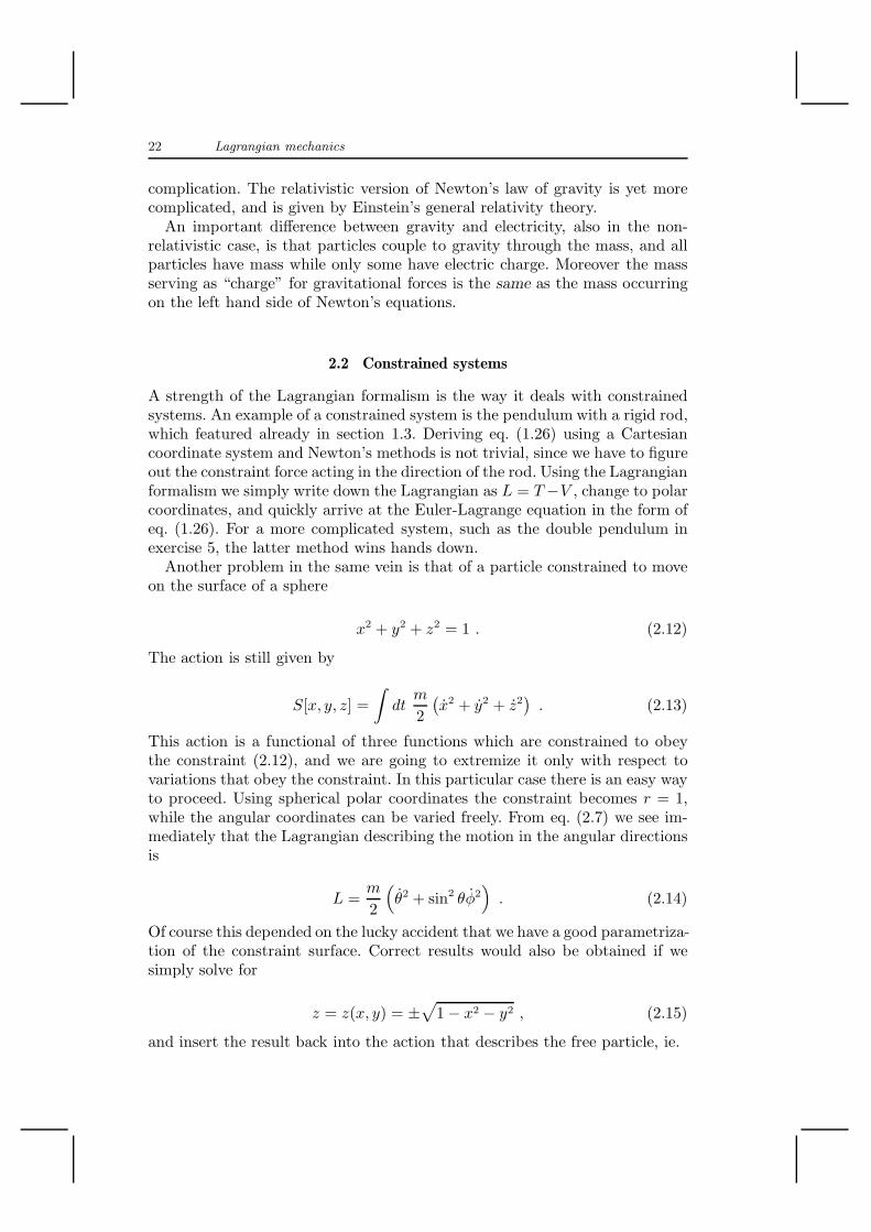
2.2 Constrained systems
A strength of the Lagrangian formalism is the way it deals with constrainedsystems. An example of a constrained system is the pendulum with a rigid rod,which featured already in section 1.3. Deriving eq. (1.26) using a Cartesiancoordinate system and Newton’s methods is not trivial, since we have to figureout the constraint force acting in the direction of the rod. Using the Lagrangianformalism we simply write down the Lagrangian as L = T−V , change to polarcoordinates, and quickly arrive at the Euler-Lagrange equation in the form ofeq. (1.26). For a more complicated system, such as the double pendulum inexercise 5, the latter method wins hands down.
Another problem in the same vein is that of a particle constrained to moveon the surface of a sphere
x2 + y2 + z2 = 1 . (2.12)
The action is still given by
S[x, y, z] =
∫
dtm
2
(
x2 + y2 + z2)
. (2.13)
This action is a functional of three functions which are constrained to obeythe constraint (2.12), and we are going to extremize it only with respect tovariations that obey the constraint. In this particular case there is an easy wayto proceed. Using spherical polar coordinates the constraint becomes r = 1,while the angular coordinates can be varied freely. From eq. (2.7) we see im-mediately that the Lagrangian describing the motion in the angular directionsis
L =m
2
(
θ2 + sin2 θφ2)
. (2.14)
Of course this depended on the lucky accident that we have a good parametriza-tion of the constraint surface. Correct results would also be obtained if wesimply solve for
z = z(x, y) = ±√
1 − x2 − y2 , (2.15)
and insert the result back into the action that describes the free particle, ie.

2.2 Constrained systems 23
S[x, y] =
∫
dtm
2
(
x2 + y2 + z(x, y)2)
. (2.16)
Now we can vary x and y freely, except that they are not allowed to exceedone in absolute value. The variations in z are now
δz = δx∂z
∂x+ δy
∂z
∂y, (2.17)
and the equations of motion can be derived at the expense of some effort.There are some unavoidable weaknesses here. From eq. (2.16) it appears as
if the configuration space were the unit disk in the plane, since x and y are notallowed to take values outside this disk. Or perhaps the configuration space istwo copies of the unit disk, since there are two branches of the square root?But the true configuration space is a sphere. What we see is a reflection ofthe known fact that it is impossible to cover a sphere with a single coordinatesystem—our equations have only a “local” validity. This kind of difficultieswill become more pronounced in the general problem we are heading for: Con-sider a Lagrangian L0 defined on an n dimensional configuration space, withcoordinates q1, . . . , qn, and suppose that the system is confined to live in the(n−m) dimensional submanifold defined by the m conditions
ΦI(q1, . . . , qn) = 0 , 1 ≤ I ≤ m . (2.18)
Derive equations of motion consistent with this requirement. One way to dothis is to solve for m of the qs, q1, . . . , qm say, by means of the m conditions(2.18), and insert the result in the action. In general this will be a lot of hardwork, and the difficulties we had with coordinatizing the sphere will recur witha vengeance.
The fact that the procedure avoids dealing with the constraint forces is aweakness too. If we try to design a pendulum in such a way that the approx-imation of a totally rigid rod holds for the kind of motion the pendulum willbe subject to, we will want to know how strong the constraint force actu-ally is. The method of Lagrange multipliers solves this problem, and at thesame time has the advantage that the difficulties with coordinatizing the con-straint surface are postponed to a later stage. The claim we will verify is this:Extremizing the action
S[q] =
∫
dt L0(q, q) (2.19)
using only variations consistent with the constraints (2.18) is equivalent toextremizing the action
S[q, λ] =
∫
dt L0(q, q) + λ1Φ1(q) + · · · + λmΦm(q) (2.20)

24 Lagrangian mechanics
under arbitrary variations of the functions q and λ. The λs are the Lagrangemultipliers, and are treated as new dynamical variables.
Indeed, when the action (2.20) is varied with respect to the λs we obtain theconstraints (2.18) as equations of motion. When we vary with respect to theqs the resulting equations will contain the otherwise undetermined Lagrangemultipliers, and it not obvious that these equations have anything to do withthe problem we wanted to consider. But they do. Consider the analogousproblem encountered in trying to find the extrema of an ordinary functionf(q) of the n variables q, subject to the m conditions Φ(q) = 0. (Remembersuppression of indices!) First suppose that we use the constraints to solvefor m of the qs—it will not matter which ones—and call them y, leavingn −m independent variables x. The extrema of f(q) may be found throughthe equations
0 = δf = δx∂xf + δy∂yf , (2.21)
where, however, the variations δy are not independent variations, but have tobe consistent with the constraints. In fact they are linear function of the δxs,given by the conditions
0 = δΦ = δx∂xΦ + δy∂yΦ . (2.22)
This equation has to be solved for δy and the result inserted into eq. (2.21),which is therefore really an expression of the form δx(∂xf +something else) =0. It does not imply ∂xf = 0.
Since δΦ = 0 for the variations we consider, nothing prevents us from rewrit-ing eq. (2.21) in the form
0 = δf = δf + λδΦ = δx(∂xf + λ∂xΦ) + δy(∂yf + λ∂yΦ) , (2.23)
where the λs are arbitrary functions. The δys are still given in terms of the δxs,so it would seem at first sight that we cannot conclude that ∂xf + λ∂xΦ = 0,but—and here comes the punch line—in fact we can, provided we choose theso far arbitrary functions λ in such a way that ∂yf + λ∂yΦ = 0. Since thedivision of the qs into xs and ys was arbitrary, we see that the “restricted” wayof finding the extrema—making variations consistent with the constraints—isequivalent to solving the n+m equations
Φ(q) = 0 ∂qf + λ∂qΦ = 0 (2.24)
for q and λ. But these are precisely the equations that we obtain from the La-grange multiplier method, in which we do not care about the constraints whilevarying the action! In all fairness though, we have not solved the equations,we have just derived them in a convenient way.
As long as the constraints depend only on q (and not on q) it is straight-forward to generalize the argument from functions to functionals. From theaction

2.2 Constrained systems 25
S[q, λ] = S0[q] +
∫
dt λΦ(q) (2.25)
we rederive the constraints, together with the equations of motion
δS
δq=δS0
δq+ λ∂qΦ = 0 . (2.26)
This is the analogue of the second equation (2.24). Written out, if L = L(q, q)and if there is only one constraint, this is
d
dt
∂L
∂qi=∂L
∂qi+ λ
∂Φ
∂qi(2.27)
Φ(q) = 0 . (2.28)
These equations have a simple interpretation. The constraint defines a surfacein configuration space. We have modified the unconstrained systems by addingan extra force term λ∂iΦ to the equations. This force is directed along thegradient of the constraint function, which means that it acts in a directionorthogonal to the constraint surface. To ensure that the trajectory is confinedto the surface we must choose the strength of the force (given by λ) in such away that this is ensured. In other words, once we have solved these equationswe know the strength of the constraint forces.
We have also refrained from committing us to any coordinate system adaptedto the specific form of the constraint surface. That this is an advantage be-comes evident when we return to the problem of the particle on a sphere,starting from the Lagrangian
L =m
2
(
x2 + y2 + z2)
+ λ(
x2 + y2 + z2 − 1)
. (2.29)
The equations of motion (in these inertial coordinates) are
mx = 2λx my = 2λy mz = 2λz . (2.30)
By inspection we see that there are three constants of the motion,
Jx = yz − zy Jy = zx− xz Jz = xy − yx . (2.31)
At this point we go over to polar coordinates, using eqs. (2.6) with r = 1. Theconstants of the motion become
Jx = −θ sinφ− φ cosφ cos θ sin θ Jy = θ cosφ− φ sinφ cos θ sin θ
(2.32)
Jz = φ sin2 θ .

26 Lagrangian mechanics
It is possible to check directly, using the equations of motion for θ and φ, thatthese are constants of the motion—but only Jz is “obviously” conserved. Thecoordinate system (θ, φ) somehow “hides” the others.
By the way, the kinetic energy can be expressed as
T =m
2
(
θ2 + φ2 sin2 θ)
=m
2
(
J2x + J2
y + J2z
)
. (2.33)
This is the angular momentum squared.So far we have dealt only with holonomic constraints, that is constraints
involving the configuration space variables only. But consider a ball movingwithout friction across a table. The configuration space has five dimensions: theposition (x, y) of the centre of mass, and three angular coordinates describingthe orientation of the ball. Now suppose instead that the ball rolls withoutslipping. If we are given the position of the centre of mass as a function of timethen the motion of the ball is fully determined, which suggests that x and y arethe “true” degrees of freedom, and that the constrained configuration space istwo dimensional. But the situation is more complicated than that (and cannotbe described by holonomic constraints). It is impossible to solve for the angularcoordinates in terms of x and y. Indeed from our experience with such thingswe know that the orientation of the ball at a given point depends on how it gotthere. Mathematically there is a constraint relating the velocity of the centreof mass to the angular velocity; the point of contact between ball and table isalways momentarily at rest.
Constraints that cannot be expressed as conditions on the configurationspace are called anholonomic. The Lagrange multiplier method can be gener-alized to handle some anholonomic constraints as well, but we will not do sohere.
2.3 Symmetries
Let us return to Newton’s Third Law. It amounts to a restriction on the kindof forces that are allowed in the second law, and implies that there exist aset of constants of the motion, namely the momenta. (The terminology is alittle unfortunate, since we will soon introduce something called “canonicalmomenta”. They are indeed identical with the conserved momenta in simplecases, but logically there need be no connection.) Constants of the motionare useful when trying to solve the equations of motion, and Emmy Noetherproved a theorem explaining when and why they exist. We present the prooffor a Lagrangian of the general form L = L(q, q), and afterwards we discuss asimple example. Let us say at the outset that the argument is quite subtle.
Consider first an arbitrary variation of the action. According to eq. (2.3)the result is
δS =
∫ t2
t1
dt δq
(
∂L
∂q− d
dt
∂L
∂q
)
+
[
δq∂L
∂q
]t2
t1
. (2.34)

2.3 Symmetries 27
In deriving the equations of motion the variations δq(t) were restricted in sucha way that the boundary terms vanish. This time we do something different.The variations are left unrestricted, but we assume that the function q(t)that we vary around obeys the Euler-Lagrange equations. Then the only non-vanishing term is the boundary term, and
δS = ǫ (Q(t2) −Q(t1)) , ǫQ(t) ≡ δq∂L
∂q. (2.35)
Here and in the following ǫ is the constant occuring in δq = ǫf , where f is anarbitrary function of t. The point is to ensure that there is nothing infinitesimalabout Q.
So far nothing has been assumed about the variations. Now suppose that,for the given Lagrangian, there exists a set of variations δq of some specifiedform
δq = δq(q, q) , (2.36)
such that for these special variations
δS = 0 . (2.37)
It is understood that the Lagrangian is such that eq. (2.37) holds as an identity,regardless of the choice of q(t), for the special variations δq. (Note that, given aLagrangian, it is not always the case that such variations exist. But sometimesthey do.)
Next comes the crux of the argument. Consider variations of the particularkind that makes eq. (2.37) hold as an identity—so that δq = ǫf is a knownfunction—and restrict attention to q(t)s that obey the equations of motion.With both these restrictions in force, we can combine eqs. (2.37) and (2.35)to conclude that
0 = δS = ǫ (Q(t2) −Q(t1)) . (2.38)
The times t1 and t2 are arbitrary, and therefore we can conclude that Q =Q(q, q) is a constant of the motion.
What this theorem does for us is to transform the problem of looking forconstants of the motion to the problem of looking for variations under whichthe variation of the action is identically zero. Before we turn to exampleswe generalize the argument slightly, and state the theorem properly. Thus,suppose that there exists a special form of δq, such that
δS =
∫ t2
t1
dtd
dtΛ(q, q) . (2.39)
Here Λ can be any function—the important and unusual thing is that theintegrand is a total time derivative. Then the quantity Q, defined by

28 Lagrangian mechanics
ǫQ(q, q) = δqi∂L
∂qi− Λ(q, q) (2.40)
is a constant of the motion. This is easy to see along the lines we followedabove.
The theorem can now be stated as follows:
Noether’s theorem: To any variation for which δS takes the form (2.39), therecorresponds a constant of the motion given by eq. (2.40).
We will have to investigate whether Lagrangians can be found for which suchvariations exist, otherwise the theorem is empty. Fortunately it is by no meansempty, indeed eventually we will see that all useful constants of the motionarise in this way.
For now, one example—but one that has many symmetries—will have tosuffice. Consider a free particle described by
L =m
2xixi . (2.41)
Since only x appears in the Lagrangian, we can choose
δxi = ǫi , (2.42)
where ǫi is independent of time. Then the variation of the action is auto-matically zero, Noether’s theorem applies, and we obtain a vector’s worth ofconserved charges
Pi =∂L
∂xi= mxi . (2.43)
We use the letter P rather than Q because this is the familiar conservedmomentum vector whose presence is postulated in Newton’s Third Law.
Another set of three conserved charges can be found easily, since
δxi = ǫijkǫjxk ⇒ δS = 0 . (2.44)
Here ǫi is again independent of t, and ǫijk is the totally anti-symmetric ep-silon tensor. Noether’s theorem now implies the existence of another conservedvector, namely
Li = ǫijkxjxk . (2.45)
This is the angular momentum vector.We know that there is at least one more conserved quantity, namely the
kinetic energy. Actually there are several, but the story now becomes a bit morecomplicated because we have to deal with variations for which the variationof the Lagrangian is a total derivative, as in eq. (2.39), rather than zero. Thus

2.3 Symmetries 29
δxi = ǫxi ⇒ δS =
∫
dtd
dt
(ǫm
2x2)
. (2.46)
Using eq. (2.40) we obtain the constant of the motion
E =m
2xixi . (2.47)
This is the conserved energy of the particle. There is yet another conservedquantity that differs from the others in being an explicit function of time—butits total time derivative vanishes since it also depends on the time dependentdynamical variables. Thus
δxi = −ǫit ⇒ δS =
∫
dtd
dt(−mǫixi) . (2.48)
Eq. (2.40) gives the conserved charge
Qi = mxi − tmxi , (2.49)
and it is easy to check that its total time derivative vanishes as a consequenceof the equations of motion. Our analysis of the free particle ends here, but wewill return to it in a moment, to show that the conserved quantities have aclear physical meaing.
What does it all mean? What does it mean for an action S[q(t)] to admitvariations δq(t) leaving the action unaffected? To see this, select a solutionq(t) of the equations of motion. We know that this gives an extremum ofthe action. Then consider q′(t) = q(t) + δq(t), where the variation is of thespecial kind that leaves the value of the action unchanged. Obviously thenS[q′(t)] = S[q(t)], so that the extremum is not an isolated point in the spaceof all qs, but rather occurs for a set of qs that can be reached from each otherby means of iteration of the special variation δq(t), In other words, given aparticular solution of the equations of motion, we can get a whole set of newsolutions if we apply the special variation, without going through the work ofsolving the equations of motion again. This leads to an important definition:
A symmetry transformation is any transformation of the space of functionsq(t) having the property that it maps solutions of the equations of motion toother solutions.
This is not a property of the individual solutions, but of the set of all solutions.The special variations occurring in the statement of Noether’s theorem areexamples of symmetry transformations. Given the converse of the statementthat we proved, namely that any constant of the motion gives rise to a specialvariation of the kind considered by Noether, we observe that any constant ofthe motion arises because of the presence of a symmetry. (There is a converseof this statement that we will come to in section 8.3.)

30 Lagrangian mechanics
Let us interpret the symmetry transformations that we found for the freeparticle, beginning with eq. (2.42). This is clearly a translation in space. There-fore momentum conservation is a consequence of translation invariance. It isimmediate that we can iterate the infinitesimal translations used in Noether’stheorem to obtain finite translations, and the statement is that given a solutionto the equations of motion all trajectories that can be obtained by translatingthis solution are solutions, too. To be definite, given that (vt, 0, 0) is a solu-tion for constant v, (a+ vt, b, c) is a solution too, for all real values of (a, b, c).Translation invariance acquires more content when used in the fashion of New-ton’s third law, which we can restate as “the action for a set of particles hastranslation symmetry”. For free particles this is automatic. When interactionsbetween two particles are added, the law becomes a restriction on the kind ofpotentials that are admitted in
L =m1
2x2
1 +m2
2x2
2 − V (x1,x2) . (2.50)
(Here I use boldface notation for the vectors because I need subscripts to labelthe particles. Always adapt notation to the circumstances!) Indeed invarianceunder (2.42) requires that
V (x1,x2) = V (x1 − x2) . (2.51)
This is a strong restriction since the function V now depends on only threevariables, as opposed to six in the general case.
Eq. (2.44) expresses the fact that the Lagrangian has rotation symmetry,while eq. (2.46) is an infinitesimal translation in time: Given a solution x(t),the function
x′(t) = x(t+ t0) = x(t) + t0x(t) + o(t20) (2.52)
is a solution too. So we can make the elegant summary that conservation ofmomentum, angular momentum and energy are consequences of symmetriesunder translations and rotations in space, together with translations in time.Eq. (2.48) expresses invariance under “boosts”, since it changes all velocitiesby a constant amount. The free particle is exceptional because we can reachevery solution by a symmetry transformation, starting from any given solution.
Having said all this, it is not true that every symmetry gives rise to aconstant of the motion. Discrete symmetries like reflections, that do not ariseby iterating an infinitesimal symmetry, are counterexamples, and we will seeanother in section 4.5.
To sum up, symmetries are important from two quite different points ofview. Given the equations they facilitate the search for solutions, but theyalso facilitate the search for the correct equations (if we believe that theyshould exhibit a certain symmetry). Noether’s theorem is a tool for discover-ing symmetries, as well as for deducing their corresponding constants of themotion.
2.3 Symmetries 31
⋄ Problem 2.1 Prove the epsilon-delta identity
ǫijkǫkmn = δimδjn − δinδjm .
What does it look like in the “cross product” notation?
⋄ Problem 2.2 Derive Lorentz’ equation from the action (2.10).
⋄ Problem 2.3 Prove that the equation
mx+ γx+ kx = 0
cannot be derived from an autonomous Lagrangian, that is to say a Lagrangian thatdoes not explicitly depend on time. Then derive the equation from a Lagrangian ofthe form L = L(x, x, t).
⋄ Problem 2.4 Consider the Lagrangian
L =1
2Mij(q)qiqj ,
where the matrix elements of Mij depend on the configuration space coordinates,and the matrix is assumed to have an inverse M−1
ij . Write down the Euler-Lagrangeequations and solve for the accelerations.
⋄ Problem 2.5 Write down the Lagrangian for a double pendulum. (The rodof the second is attached to the bob of the first. Bobs are heavy, the rigid rods not.)How many constants of the motion can you find?
⋄ Problem 2.6 TakeN positive numbers summing to one, p1+p2+· · ·+pN = 1.Their geometric mean is defined as (p1p2 · · · · · pN )1/N . What is the maximum of thegeometric mean?
⋄ Problem 2.7 Check that the result from eq. (2.17) is the same as thatobtained from the recipe in eq. (2.22). Beware of changes in notation!
⋄ Problem 2.8 Consider a particle with kinetic energy T = m(x2 + y2− z2)/2,and constrain it to the hyperboloid x2 + y2 − z2 = −1, z > 0. Treat this both withcoordinates adapted to the hyperboloid and with the Lagrange multiplier method.Show that the kinetic energy is positive and find three constants of the motion.
⋄ Problem 2.9 In the brachistrone problem one considers a particle slidingalong a curve in the x-z-plane (z is vertical) under the influence of gravity. Choosethis curve so that the time of descent from (x, z) = (x0, z0) to the origin is minimal.
⋄ Problem 2.10 Given a mechanical system for which you have identified akinetic energy T = T (q, q) and a potential energy V = V (q). Let Noether’s theoremtell you under what conditions on the function T (q, q) the equations E = T + V andL = T − V are consistent with each other.
⋄ Problem 2.11 Consider the Lagrangian

32 Lagrangian mechanics
L =1
2q2 − λqn ,
where λ is a real number and n is an integer. Determine those values of n for whichthe Lagrangian transforms into a total derivative under
δq = ǫ(
tq − q
2
)
.
This is known as conformal symmetry.
⋄ Problem 2.12 Show that the Lagrangian (2.50), under the restriction (2.51),transforms into a total derivative under the transformation
δx1 = δx2 = −vt . (2.53)
Give a physical interpretation of the corresponding Noether charge.
⋄ Problem 2.13 For a free particle, consider the action integral
S =
∫ t2
t1
m
2x2dt .
Evaluate this integral for an x(t) that solves the equations of motion, and express theanswer as a function of t1, t2, and the initial and final positions x1 and x2. Repeatthe exercise for a harmonic oscillator.

3 Interlude: Conic sections
The theory of conic sections was one of the crowning achievements of theGreeks. After Descartes, it has become a habit to think of an ellipse as the setof points that obey
x2
a2+y2
b2= 1 . (3.1)
However, the equation that we come across when we solve the gravitationaltwo-body problem is
p
r= 1 + e cosφ . (3.2)
If you do not recognize it, the following account may be helpful.By definition a conic section is the intersection of a circular cone with a
a plane. The straight lines running through the apex of the cone are calledits generators—and we will consider a cone that extends in both directionsfrom its apex. If you like, it is the set of one dimensional subspaces in a threedimensional vector space. Generically, the plane will intersect the cone in sucha way that every generator crosses the plane once, or in such a way that exactlytwo of the generators miss the plane. Apollonius proved that the intersection isan ellipse in the first case, and a hyperbola in the second. There is a borderlinecase when exactly one generator is missing. Then the intersection is a parabola.We ignore the uninteresting case when the plane goes through the apex of thecone.
This is all very easy if we use the machinery of analytic geometry. Forsimplicity, choose a cone with circular base, symmetry axis orthogonal to thebase, and opening angle 90 degrees. It consists of all points obeying
x2 + y2 − z2 = 0 . (3.3)
Without loss of generality, the plane can be described by
cx+ z = d . (3.4)
A small calculation shows that the intersection of these two surfaces is either

34 Interlude: Conic sections
Figure 3.1. A vertical cross section through Apollonius’ proof—but to under-stand the proof you have to think in three dimensions.
an ellipse, a hyperbola, or a parabola—provided you recognize their equations,as I assume. The section is a circle if c = 0 and a parabola if c = ±1.
It is an interesting exercise to prove this in the style of Apollonius. Let thecone have arbitrary opening angle. Take the case when the plane intersectsevery generator once in the upper half of the cone. Place two spheres insidethe cone, one above and one below the plane, and let them grow until eachtouches the plane in a point and the cone in a circle. (See Fig. 3.1.) This clearlydefines the spheres uniquely. Denote the points by F1 and F2, and the circlesby C1 and C2. Now consider a point P in the intersection of the cone and theplane. The generator passing through P intersects the circles C1 and C2 inthe points Q1 and Q2. Now the trick is to prove that the distance PF1 equalsthe distance PQ1, and similarly the distance PF2 equals the distance PQ2.This is true because the distances measure the lengths of two line segmentsthat are tangent to the sphere and end at the same point. It then follows thatthe sum of the distances PF1 and PF2 is constant and equal to the length ofthe segment of the generator between the circles C1 and C2, independently ofwhich point P on the intersection we choose. This property defines the ellipse.This is the proof that the intersection between the cone and the plane is anellipse with its foci at F1 and F2. If you are unable to see this, consult an oldfashioned geometry book.
For our purposes it is convenient to define the ellipse somewhat differently.An ellipse of eccentricity e < 1 can be defined as the set of points whosedistance from a given point, called a focus, is e times the distance to a straightline, called a directrix. For the circle e = 0, and the directrix is at infinity.
The latus rectum of an ellipse is a chord through the focus parallel to thedirectrix, and has length 2p. Now place the origin of a coordinate system atthat focus, with the x-axis pointing towards the directrix. The distance of apoint on the ellipse to the focus is
r = e(distance to the directrix) = e(p
e− x)
. (3.5)

Interlude: Conic sections 35
Figure 3.2. An ellipse, with eccentricity 0.58, semi-major axis a, semi-minoraxis b, and latus rectum p. The directrix appears on the right. The distancebetween the centre and the focus is 0.58a.
(To see this, note that the distance from the focus to the directrix is p/e.)Otherwise expressed
r = p− er cosφ ⇔ p
r= 1 + e cos φ , (3.6)
where φ = 0 gives the point closest to the directrix. For a general point on theellipse we find
x2 + y2 = r2 = (p− ex)2 ⇔ (x+ ea)2
a2+y2
b2= 1 , (3.7)
where
a ≡ p
1 − e2b2 = pa = (1 − e2)a2 . (3.8)
The major axis of the ellipse has length 2a, and the minor axis has length 2b.The eccentricity is given in terms of these by
e2 =a2 − b2
a2. (3.9)
Finally the distance between the centre and the focus equals ea. To see thiswe set φ = 0 and φ = π in eq. (3.6), and calculate
r(π) − r(0)
2=p
2
(
1
1 − e− 1
1 + e
)
= ea . (3.10)
For some further information consult exercise 1.

36 Interlude: Conic sections
Similar treatments can be given for the hyperbola, for which e > 1, and forthe parabola, for which e = 1.
In our study of the two-body problem we will find it interesting to relatean ellipse centred at a focus to an ellipse centred at the origin. The latter isdescribed in Cartesian coordinates by the complex trajectory
w(t) = a cos t+ ib sin t . (3.11)
The parameter t must not be confused with the angle φ between the radiusvector and the x-axis. Surprisingly, if we square this ellipse we obtain an ellipsewith its focus at the origin. First we see that
Z(t) = w2 =a2 + b2
2cos 2t+ iab sin 2t+
a2 − b2
2. (3.12)
Using eq. (3.9) we see that the eccentricity E of the new ellipse is
E =a2 − b2
a2 + b2. (3.13)
So we can rewrite the equation for the new ellipse as
Z(t) = A cos 2t+ iB sin 2t+EA , (3.14)
where
A ≡ a2 + b2
2, B ≡ ab , EA =
√A2 −B2 . (3.15)
E is the eccentricity of an ellipse with semi-major axis A and semi-minor axisB, and consequently EA is the distance between its focus and its centre. Thisis again an ellipse, but shifted to be centred at one of its foci—in the sensethat the angle is now seen from a focus—and traversed twice as the originalellipse is traversed once. When we put these observations to use in section 4.3,it will be important that every ellipse described on the form (3.14) can beobtained in this way from a function w(t), with suitable choices of a and b.
This trick was introduced by Karl Bohlin, working at the Pulkovo observa-tory in Russia in 1911. His point was that the transformation w =
√Z is not
analytic at the origin. This enabled him to deal with collisions between pointparticles, thought of as limiting cases of elliptical orbits whose eccentricityapproaches 1. At the collision the particle presumably reverses its direction,but this is a rather singular occurence. In terms of the variable w it is anundramatic event.
⋄ Problem 3.1 Using the definition in terms of the directrix, prove that thesum of the distances from the two foci to a point on an ellipse is constant.

Interlude: Conic sections 37
⋄ Problem 3.2 Prove that the area of an ellipse equals πab. Set up an expressionthat gives the circumference of the ellipse.
⋄ Problem 3.3 Place a lamp at one focus of an ellipse, and let the circumferenceof the ellipse act as a mirror. Prove that all planar light rays reconverge at the sametime at the other focus. Try to do this in two different ways: by means of a calculation,and by means of an argument that makes it all obvious.
⋄ Problem 3.4 For the parabola y = x2, where is its focus? Its directrix?
⋄ Problem 3.5 Consider a trajectory that is a straight line through the originin the w-plane. Apply Bohlin’s trick. What trajectory results in the Z–plane?

4 The central force two-body problem
Johannes Kepler spent his life pondering the observations of the solar systemmade by Tycho Brahe, and found that the motion of the planets around thesun follows three simple rules:
1. A planet moves along an ellipse with the sun in one of the foci.2. The radius vector covers equal areas in equal times.3. The square of the period of all the planets is proportional to the cube oftheir major axes.
To appreciate Kepler’s work fully, note that there are important facts aboutthe solar system (such as what the distances are) that do not follow simplerules. Moreover the observational data gave the planetary orbits projected ona sphere centred at a point which itself moves along an ellipse around the sun,so it was not obvious that they admitted of a simple description at all.
Kepler was clear about his aims: “My goal is to show that the heavenlymachine is not a kind of divine living being but similar to a clockwork inso far as almost all the manifold motions are taken care of by one singleabsolutely simple magnetic bodily force, as in a clockwork all motion is takencare of by a simple weight.”1 Eventually Newton derived Kepler’s laws from hisown Laws, with the necessary assumption that the force between the planetsand the sun is directed along the radius vector (the force is central) and isinversely proportional to the square of the distance. This remains the numberone success story of physics, so we should be clear about why this is so. NaivelyKepler’s laws may seem simpler than Newton’s, but this is not so, for at leasttwo reasons. One is that Newton’s laws unify a large body of phenomena, fromthe motion of planets to the falling of stones close to the Earth. The otherreason is that improved observations reveal that Kepler’s laws are not quiteexact, and the corrections can be worked out mathematically from Newton’slaws.
For Mercury (which is hard to observe) the eccentricity e = 0.21, for theEarth e = 0.02, and for Mars e = 0.09. Kepler’s main concern was with Mars.If e = 0 the ellipse becomes a circle. Unbound motion through the solar systemis described by hyperbolas with e > 1, but Kepler did not know this.
1 J. Kepler, letter to Herwart von Hohenburg, February 10, 1605.

4.1 The problem and its formal solution 39
4.1 The problem and its formal solution
We want to derive Kepler’s laws. As an approximation we assume that itsuffices to treat the planets independently of each other. Moreover we assumethat the precise shapes of the sun and the planets are unimportant and thatthey can be approximated as being pointlike. Later on, we can go back tothese assumptions and see if we can relax them—this will give the correctionsreferred to above.
Actually, in the Principia, Newton proved a comfortable theorem: The grav-itational force acting on a particle outside a spherical body of total mass m isidentical to that from a particle of mass m sitting at the centre of the body.This is a consequence of the inverse square law, and shows that our secondassumption is exact for spherical bodies. Newton also proved that the inversesquare law implies that there is no force at all on a particle inside a sphericalshell, regardless of the mass of the shell. Concerning the first assumption, aquick estimate shows that the force due to Jupiter acting on Venus is about2 · 10−5 times that due to the Sun, and the influence of the other planets iseven smaller. So it makes sense to proceed.
We have decided that the configuration space of our problem has six dimen-sions, spanned by the positions of the sun (X) and one planet (xP ), and wetry the Lagrangian
L =M
2XiXi +
mp
2xPixPi − V (X,xP ) . (4.1)
Depending on the form of the function V we may have to exclude the pointsX = xP from the configuration space—we insist that the function V takesfinite values only as a function on configuration space. Anyway this will give sixcoupled second order differential equations. In general they will not admit anysimple solutions. Kepler’s work implies that the solutions should be simple,so we try to build some symmetries into the problem. We aim for at leastsix conserved quantitities, one for each degree of freedom, since this shouldresult in a soluble problem. Conservation of momentum and energy is alreadypostulated, so we need two more. The answer is rotational symmetry. It is notan objection that an ellipse is not symmetric under rotations. All we need isthat if a particular ellipse is a solution, then any ellipse which can be obtainedfrom it by means of rotations is a solution too, even if there is no planet movingalong it due to the choice of initial conditions. It might seem that rotationalsymmetry is overdoing it, since it will yield three conserved quantitities, but—for reasons fully explained by the theory of integrable systems, see chapter10—only two of these are really useful.
With translational and rotational symmetry in place, we find
V (X,xP ) = V (X − xP ) = V (|X − xP |) . (4.2)
This works for any function V of one variable. Next we introduce coordinatesxi = xPi−Xi which are invariant under translations, together with coordinates

40 The central force two-body problem
describing the centre of mass. Then the centre of mass coordinates decouple,and their equations can be solved and set aside. There remains a Lagrangianfor a one-body problem, involving only three degrees of freedom:
L =m
2x2i − V (|x|) . (4.3)
Here m is the reduced mass
m =Mmp
M +mp
. (4.4)
The reduced mass is almost equal to the mass of the planet since the sun isvery heavy in comparison. The coordinate xi vanishes at the centre of mass ofthe system, which is well inside the sun, and can be approximately identifiedwith the centre of the sun. This maneouvre should be familiar from elementarymechanics, I just want to emphasize that it is translational symmetry in action.
Rotational symmetry implies the existence of a conserved vector
Li = mǫijkxjxk . (4.5)
This vector is orthogonal to both x and x, which means that the motionis confined to a plane orthogonal to the angular momentum vector. We aredown to a two dimensional configuration space. To take maximal advantage ofspherical symmetry we introduce spherical polar coordinates, chosen so thatthe plane containing the orbit is at θ = π/2. The Lagrangian simplifies to
L =m
2(r2 + r2φ2) − V (r) . (4.6)
We have used the constant direction of the angular momentum vector. Butits magnitude is constant too. This happens because the Lagrangian (4.6) isinvariant under translations in the angle φ. Using Noether’s theorem we findthe constant of the motion
l =∂L
∂φ= mr2φ . (4.7)
This equation is of considerable interest in itself. It says that
A =r2φ
2=
l
2m= constant , (4.8)
where A is the area covered by the radius vector per unit time. But this isKepler’s Second Law, which therefore holds for all central forces. We are onthe right track!
Together with Kepler’s second law, energy conservation is enough to solvethe problem. Using eq. (4.7) the conserved energy is

4.2 Existence and stability of circular orbits 41
E =m
2
(
r2 + r2φ2)
+ V (r) =mr2
2+
l2
2mr2+ V (r) = constant . (4.9)
This gives the formal solution
dt =dr
√
2m
(
E − l2
2mr2− V (r)
)
. (4.10)
It may or may not, depending on our choice of V (r), be possible to do theintegral in terms of elementary functions, but anyway this equation determinesthe function r(t), and hence solves the problem. To find φ(t) we combine eqs.(4.7) and (4.10), and get
dφ =ldt
mr2=
ldr
r2
√
2m(
E − l2
2mr2− V (r)
)
. (4.11)
This equation determines φ(r(t)), and the central force problem is therebyfully solved at the formal level. If we are only interested in the form of theorbits, and not the time development, eq. (4.11) is all we need—it will give usφ(r), and after inversion r(φ), which is the equation for the form of the orbit.
4.2 Existence and stability of circular orbits
There is a special kind of solution that we can look for directly, with no greatexpense of effort, namely circular orbits. From the expression (4.9) we seethat the two body central force problem has been reduced to one dimensionalmotion in the effective potential
Veff (r) =l2
2mr2+ V (r) . (4.12)
A simple case is V (r) = 0, i.e. no force at all. In the effective one dimensionalproblem this corresponds to a repulsive Veff—the particle comes in from in-finity, reaches a minimum value of r, and then disappears to infinity again. Ifwe want a bound orbit the potential V (r) must be attractive.
A circular orbit is one for which r = 0 identically, which means that theparticle is sitting at the bottom of the effective potential—if it does have abottom. The radius r of the circular orbit must obey
V ′eff (r) = 0 . (4.13)
If this happens at a local maximum of Veff the solution is unstable, andunlikely to be realized in Nature. The orbit is stable under small perturbationsif and only if
42 The central force two-body problem
V ′′eff > 0 (4.14)
at the value of r for which V ′eff = 0.
We look into these equations for the choice
V (r) = −krβ ⇒ Veff (r) =l2
2mr2− krβ , (4.15)
with β arbitrary (except that we exclude the obviously special case β = −2).The radius of the circular orbit is found to be
r =
(
− l2
βkm
)1
β+2
. (4.16)
This makes sense only if l2 6= 0—a question of initial conditions—and βk < 0.Then the second derivative will be positive if and only if
β > −2 . (4.17)
Thus stability of the circular orbit requires that the force does not fall off tooquickly with distance.
There is still the question whether small departures from the circular orbitwill give rise to ellipses, or to something more complicated. This is really aquestion about the ratio between the time it takes for the planet to completea full revolution in φ, to the time it takes to complete a full oscillation in r. Ifthe orbit is an ellipse centred at a focus these times must be equal, and thisis likely to happen only for a very special V (r). Compare the discussion ofLissajous figures in section 1.3. For general bounded motion the amount bywhich the perihelion precesses during one period of the radial motion followsfrom eq. (4.11). It is
∆φ = 2
∫ rmax
rmin
ldr
r2√
2m (E − Veff (r)). (4.18)
For the planets, Kepler’s first law requires that ∆φ = 2π.A final comment: if we do choose the exponent β = −1 we have the problem
that the energy is unbounded from below. We now see that this problem cannotbe too serious, because
Veff (r) =l2
2mr2− k
r(4.19)
is in fact bounded from below whenever l 6= 0. The case when l = 0 is indeedtroublesome from a physical point of view: the two bodies will collide, and wedo not have a prescription for what is to happen after the collision. The caseof coinciding particles is not included in our configuration space.

4.3 Kepler’s First Law 43
4.3 Kepler’s First Law
What force laws are consistent with Kepler’s First Law? Hooke’s law does giveelliptical orbits. This is most easily seen by transforming the Lagrangian backto Cartesian coordinates:
L =m
2(r2 + r2φ2) − kr2 =
m
2(x2 + y2) − k(x2 + y2) . (4.20)
This is two harmonic oscillators of equal frequencies, and the correspondingLissajous figures are indeed ellipses. They are not the right kind of ellipseshowever, since they are centred at the origin. Let us call them Hooke ellipses.They can be related to Kepler ellipses (centred at a focus) by means of Bohlin’strick (chapter 3). If
w = |w|eiφ = a cos t+ ib sin t (4.21)
is a Hooke ellipse, then
Z = w2 = |w|2e2iφ =a2 − b2
2+a2 + b2
2cos 2t+ iab sin 2t . (4.22)
This is indeed an ellipse centred at a focus, as we saw in chapter 3. For theHooke ellipse w(t) we know that the force law is
w = −w ⇒ |w|2 + |w|2 = 2ǫ . (4.23)
Moreover Kepler’s second law holds, so that
|w|2 dφdt
= constant . (4.24)
This relates the parameter t to the angle φ between the radius vector and themajor axis. The idea now is to introduce a new time τ , related to t in such away that Kepler’s second law holds also for the ellipse we get when we squarethe Hooke ellipse. Thus, remembering that the phase of Z is 2φ, we require
2|Z|2 dφdτ
= constant . (4.25)
A suitable choice of the two constants gives the desired relation
dτ
dt=
|Z|2|w|2 = |w|2 ⇔ d
dτ=
1
|w|2d
dt. (4.26)
At this point then we have obtained a function Z(τ) that describes motion inaccordance with Kepler’s First and Second Laws. It only remains to investi-gate what differential equation it obeys. But using eqs. (4.23) this is a simplecalculation:

44 The central force two-body problem
d2Z
dτ 2=
1
|w|2d
dt
(
1
|w|2dw2
dt
)
=2
|w|2d
dt
(
w
w
)
= · · · = −4ǫZ
|Z|3 , (4.27)
where ǫ is the constant energy of the Hooke ellipse. This is precisely Newton’sforce law for gravity. So we conclude that Kepler’s First and Second Lawstogether imply the inverse square law, with the potential
V (r) = −kr. (4.28)
We simply calculated the force law, and conclude that Kepler’s First andSecond Laws hold if and only if the inverse square law holds for the force.The argument is watertight because Bohlin’s trick can be used to parametrizeevery Kepler ellipse in this convenient way.2
To confirm our conclusion let us go back to eq. (4.11), which gives a formalsolution for the form of the orbit. We choose eq. (4.28) for V (r), and we alsoperform the substitution
u =1
r⇒ du = −dr
r2. (4.29)
The result is
dφ = − ldu√2mE − l2u2 + 2mku
. (4.30)
This defines u as a trigonometric function of φ, with the energy E < 0 andthe phase φ0 as undetermined integation constants. In fact
φ = φ0 − arccosl2umk
− 1√
1 + 2El2
mk2
. (4.31)
Inverting this, and cleaning up the answer a little, we obtain
l2
mkr=l2u
mk= 1 +
√
1 +2El2
mk2cos (φ− φ0) . (4.32)
The constant φ0 is the value of the coordinate φ for which the planet is atits perihelion, that is when it is closest to the sun. Comparing to eq. (3.6) weread off that the eccentricity of the ellipse is
e =
√
1 +2El2
mk2. (4.33)
The semi-major axis of the ellipse is
2 For a better description of this beautiful argument, see V. I. Arnold: Huygens and Barrow, Newtonand Hooke, Springer 1990.

4.4 Kepler’s Third Law 45
a =p
1 − e2= − l2
mk
mk2
2El2=
k
2|E| . (4.34)
The solution remains valid also for E > 0, in which case it describes a hy-perbola with e > 1. Physically this is an unbound trajectory, like that of aspaceship heading for the stars.
4.4 Kepler’s Third Law
Kepler’s Third Law awaits proof. If you recall the basic facts about ellipsesthe following is easy: since the areal velocity is constant the period T is simplyrelated to the area of the ellipse. Starting with eq. (4.8) and recalling exercise3.2 we obtain
l
2mT = A = πab . (4.35)
Remembering that b2 = ap, and using eq. (4.32) to identify the latus rectump, gives
T 2 =4π2m2a3p
l2= 4π2m
ka3 . (4.36)
This is Kepler’s Third Law, since k = GmM so that the proportionalityconstant is independent of what planet we are looking at, to the approximationthat we can take M equal to the mass of the Sun.
Here is a more involved proof, using the full force of our solution (4.10). Werewrite it using our expressions for a and e:
dt =
√
ma
k
rdr√
− l2
2m|E|+ 2ar − r2
=
√
ma
k
rdr√
a2e2 − (r − a)2. (4.37)
We can do the integral if we can find a substitution that simplifies the integral
∫ r rdr√
1 − (r − 1)2. (4.38)
Such a substitution is readily found. Reinserting the constants we set
r = a+ ae cos σ (4.39)
Now we can do the integral. With a suitable choice of the integration constantwe obtain
t =
√
ma3
k(σ + e sinσ) . (4.40)

46 The central force two-body problem
Taken together, eqs. (4.39-4.40) provide a parametric representation of theorbit, and we can read off its period
T = 2π
√
ma3
k. (4.41)
This is Kepler’s Third Law once again.
4.5 Self-similarity and the virial theorem
Kepler’s Third Law says that, given a solution, one can simply enlarge it to getanother solution—provided one also slows down the rate at which things arehappening. It is really a consequence of mechanical similarity or self-similarity,a kind of symmetry not covered by Noether’s theorem. It arises as follows. Takethe Lagrangian
L =m
2
(
dq
dt
)2
− V (q) , (4.42)
where we do not use the dot notation because we will soon have two differenttime parameters to reckon with. Assume that the potential is homogeneous
of degree β, meaning that there exists a real number β such that for any realnon-zero number λ
V (λq) = λβV (q) . (4.43)
There could be several variables qi. For simplicity I write only q. Let us alsochange the time scale, and define a new function q′ by
q(t) → q′(t′) = λq(t) , t′ = λ2−β
2 t . (4.44)
It follows that
dq′
dt′=dt
dt′d
dt(λq(t)) = λ
β
2dq
dt. (4.45)
We can now check that our rescalings represent a symmetry because, underthis transformation,
L
(
q,dq
dt
)
→ L
(
q′,dq′
dt′
)
= λβL
(
q,dq
dt
)
. (4.46)
This has the effect of changing the value of the action with a constant factor,and it follows that q′(t′) is an extremum of S[q′(t′)] if q(t) is an extremum ofS[q(t)]. In this sense rescaling is a symmetry of the action. (Compare problem2.11. If you find the argument difficult, you can check directly that q′(t′) is asolution whenever q(t) is.)

4.5 Self-similarity and the virial theorem 47
The harmonic oscillator has a potential V ∼ q2, homogeneous with β = 2.Scaling symmetry is present with t′ = t. Given a solution q(t) there is anothersolution that is a blown up version of this, with amplitude a factor of λ larger.Because t = t′ the period of the oscillations are unaffected by the scaling,and we see—without looking at any explicit solutions—that the period ofthe oscillations are independent of their amplitudes. Galilei first made thisobservation while celebrating mass in the cathedral of Pisa.
Newton’s law of gravity uses a homogeneous potential with β = −1, sosimilarity holds with t → t′ = λ3/2t. Two ellipses with the same shape (andthe planetary orbits are all close to circular) will therefore have their periodsand their axes related by
R→ R′ = λR T → T ′ = λ3/2T ⇒ T ′2
T 2=R′3
R3. (4.47)
This is Kepler’s Third Law for the third time.Another dramatic theorem can be proved for self-similar systems. It is called
the Virial Theorem, and relates the time averages of the kinetic and potentialenergies to each other. If it exists, the time average of a function f(t) is definedby
〈f〉 ≡ limt→∞
1
t− t0
∫ t
t0
dt′ f(t′) . (4.48)
For the argument to follow it is important that the time average of the deriva-tive of a bounded function is zero, i.e.
⟨
df
dt
⟩
= limt→∞
1
t(f(t) − f(t0)) = 0 (4.49)
whenever f(t) <∞ for all t.We are ready to study the time average of the kinetic energy, given the
assumptions that the system obeys Newton’s law
mxi = −∂iV (x) , (4.50)
that the potential is homogeneous of degree β, that the motion is boundedin space, and that the velocities are everywhere finite. On the other hand weare not restricting the index i. It could run between 1 ≤ i ≤ 3N , in whichcase we are actually studying an N -body problem; this could be a cluster ofgalaxies under the tentative assumption that the cluster is a bound system, orit could be 1023 atoms confined in a box. For the argument we will need Euler’stheorem on homogeneous functions. Regardless of the number of variables itstates that
V (λx) = λβV (x) ⇒ xi∂iV (x) = βV (x) . (4.51)
(Proof: Take the derivative with respect to λ, and then set λ = 1.)

48 The central force two-body problem
Now the calculation is easy:
2 〈T 〉 =⟨
mx2⟩
=
⟨
d
dt(mxixi) −mxixi
⟩
= −〈ximxi〉 =
(4.52)
= 〈xi∂iV (x)〉 = β 〈V (x)〉 .This is the conclusion we were after.
For bounded motion in homogeneous potentials
2 〈T 〉 = β 〈V 〉 , (4.53)
where β is the degree of homogeneity of V (x).
For the inverse square law the virial theorem implies that
〈2T + V 〉 = 0 ⇒ 〈E〉 = 〈T + V 〉 = −〈T 〉 ≤ 0 . (4.54)
This is the familiar fact that motion bounded by gravity can take place onlyif the total energy is negative. For the harmonic oscillator we deduce that thetime averages 〈T 〉 and 〈V 〉 are equal.
The virial theorem has been used by astronomers to estimate the massesof clusters of stars and clusters of galaxies, assuming that they are gravita-tionally bound. This led to the first evidence for dark matter.3 Note also thecounterintuitive fact that if energy leaves a self-gravitating cluster of particlesits energy 〈E〉 becomes more negative, which means that its average kineticenergy 〈T 〉 grows. In some sense the “gas” becomes hotter when energy is lost.
The calculation in eq. (4.52) is of interest even for non-potential forces, ifwe break it off after the first line:
2 〈T 〉 = −〈xiFi〉 . (4.55)
If the forces are the constraint forces keeping an ideal gas contained inside abox, we can use this relation to deduce the ideal gas law. We turn the suminto an integral, recall the definition of the pressure P as force per unit area,and apply Gauss’ law to the result:
2 〈T 〉 = P
∫
dAixi = P
∫
dV ∂ixi = 3PV . (4.56)
If we are willing to identify 〈T 〉 with (a factor times) the temperature T weobtain
3 The pioneering work on the Coma cluster is described, very readably, in F. Zwicky, On the Massesof Nebulae, and Clusters of Nebulae, Astrophys. J. 86 (1937) 217. Zwicky did overestimate theamount of dark matter, largely because he was assuming the cluster to be much closer to us thanit actually is, but his methods were sound and his basic conclusion correct.

4.6 The three-body problem 49
PV = RT . (4.57)
This is Boyle’s Law for ideal gases.
4.6 The three-body problem
The three-body problem—three masses interacting according to Newton’s Lawof Gravity—is not soluble in the sense that the two-body problem is. Thenumber of conserved quantities is the same in both problems, and for thenine degrees of freedom in the three-body problem this is not enough. Butthe three-body problem is very important, and in fact motivated many of thedevelopments that we will come to later on.
A natural first step is to look for special exact solutions, which may be usedas starting points for perturbation theory, or in other ways. An interesting ex-ample was found by Lagrange. Let us begin by assuming that the motion takesplace in a plane, and use complex numbers zi(t) to denote the trajectories. Theequations are
z1 = −m2
z1 − z2|z1 − z2|3
−m3
z1 − z3|z1 − z3|3
z2 = −m3
z2 − z3|z2 − z3|3
−m1
z2 − z1|z2 − z1|3
(4.58)
z3 = −m1
z3 − z1|z3 − z1|3
−m2
z3 − z2|z3 − z2|2
.
We assume that the centre of mass is at rest,
m1z1 +m2z2 +m3z3 = 0 . (4.59)
The particles form a triangle, with sides represented by
w1 = z3 − z2 , w2 = z1 − z3 , w3 = z2 − z1 . (4.60)
It turns out to be convenient to rewrite the equations of motion in terms ofthese variables. A small calculation shows them to take the form
w1 = −m w1
|w1|3+m1a
w2 = −m w2
|w2|3+m2a (4.61)
w3 = −m w3
|w3|3+m3a ,
where m = m1 +m2 +m3 and

50 The central force two-body problem
Figure 4.1. The two stable Lagrange points in Jupiter’s orbit. The Greek andTrojan asteroids lie within roughly one astronomical unit from the Lagrangepoints.
a =w1
|w1|3+
w2
|w2|3+
w3
|w3|3. (4.62)
This time we are looking for a special solution, not at the general case. So letus assume that the triangle is an equilateral one,
w2 = e2πi/3w1 , w3 = e4πi/3w1 . (4.63)
A glance at eqs. (4.61) shows that this property can be preserved in time.Then we have that a = 0, and the only equation we need to solve is
w1 = −m w1
|w1|3. (4.64)
This we know how to do.To interpret the solution, solve for
mz1 = m3w2 −m2w3 ⇒ m2|z1|2 = (m22 +m2m3 +m2
3)|w1|2 (4.65)
and so on. A small calculation then shows that
z1 = −(m22 +m2m3 +m2
3)32
m2
z1|z1|3
, (4.66)
and similarly for the other two particles. Hence the particles are all beingaccelerated towards their common center of mass, with “effective masses” thattake an unexpected form. Each individual particle travels on an ellipse, butthe tree of them do so in unison, in such a way that they always span anequilateral triangle.
A special case of this solution is of considerable physical interest. Let oneof the particles have negligibly small mass. Then the remaining pair trace out

4.6 The three-body problem 51
the same orbits that they would follow in the absence of the third member.Nevertheless the three particles span an equilateral triangle. This is the originof the two Lagrange points on the orbit of a planet, where small bodies may sit.To draw this conclusion we should also investigate whether the exact solutionis stable under small perturbations. This turns out to be the case.
The Lagrange points we have found are called L4 and L5, since there isanother set of three equilibria on the axis through the two bodies—althoughthey are of less interest since they are unstable. About a thousand asteroidshave been found close to the Lagrange points L4 and L5 on the orbit of Jupiter.They are known as the Greek and Trojan asteroids (with names taken fromHomeros). It has been observed that the Earth’s Lagrange points are suitableplaces where an alien civilisation could place a satellite surveying the Earth;however, when the STEREO spacecrafts passed through (in 2009) they foundnothing of the sort.
But what can we say about the three-body problem in general? To celebratethe sixtieth anniversary of King Oscar II of Sweden and Norway a large prizewas offered for a solution to the following problem: “For a system of arbi-trarily many mass points that attract each other according to Newton’s laws,assuming that no two points ever collide, give the coordinates of the individualpoints for all time as the sum of a uniformly convergent series whose termsare made up of known functions.” The prize was awarded to Henri Poincare,who did not solve the problem as stated. Instead he laid the foundations ofthe modern theory of dynamical systems, including chaotic behaviour. For thethree-body problem a solution was in fact found by Karl F. Sundman in 1912.He did express a generic solution as a uniformly convergent power series int1/3. The catch is that the series converges very slowly. It is estimated that,in order to get useful information, one would have to sum the first 108000000
terms. Hence the interest in the exact general solution dwindled from thatpoint in.
With the advent of the computer it has become possible to follow a largenumber of solutions to the three body problem on the screen, with no specialeffort. The zoo of solutions include ones where the third body escapes fromthe system, leaving the remaining pair more tightly bound than before.
⋄ Problem 4.1 Solve Lorentz’ equation for a charged particle moving in aconstant magnetic field.
⋄ Problem 4.2 The conservation of angular momentum is used in the gravi-tational two body problem to show that the trajectory is confined to a plane. Nowconsider an electrically charged particle moving in the electromagnetic field of a mag-netic monopole, that is to say a hypothetical particle which, if placed at the origin,gives rise to the magnetic field
Bi = bxir3
.
Here b is the magnetic charge of the monopole, and the electrically charged particle

52 The central force two-body problem
obeys Lorentz’ Law. Compute the time derivative of the particle’s angular momentum.Find a conserved quantity which is a modified version of the angular momentum. Usethe existence of this quantity, and the result of ex. 1, to qualitatively describe thetrajectory of the particle.
⋄ Problem 4.3 Consider the Earth-Moon system. Because of the tides somedissipation of energy takes place. How does this affect the distance of the moon fromthe earth?
⋄ Problem 4.4 Consider the Yukawa potential
V (r) = −k e−µr
r, k > 0 , µ > 0 .
What can you say about the existence and stability of circular orbits?
⋄ Problem 4.5 In the theory of black holes one encounters the followingequation for particles orbiting the black hole,
r2 +
(
1 − 2m
r
)(
L2
r2+ 1
)
= E2 ,
where r(t) is related to the distance to the event horizon at r = 2m, t is related totime, m is the mass of the black hole, E is the energy of the particle, and L its angularmomentum. The equations make sense only if r > 2m. You can choose L and E freely.Compute the smallest possible value of r for which a (marginally) stable circular orbit(with r = constant) exists. A warning to the uninitiated is that relativistic units areused, so that the velocity of light and Newton’s constant are set to 1.
⋄ Problem 4.6 If the Sun is flattened at its poles it will have a quadrupolemoment, and the potential is
V (r) = −kr
+q
r3.
The orbits will no longer be closed. Compute the angle by which the perihelion movesduring one revolution, to first order in q.
⋄ Problem 4.7 For the Newtonian potential (4.28) the two body problemadmits an additional conserved vector
Mi = ǫijkxjLk −k
rxi .
This is known as the Runge-Lenz vector. Check that it is indeed conserved. In whatdirection does it point?
⋄ Problem 4.8 The mass of Jupiter is 2 ·1027 kg and its distance from the Sunis 8 · 1011 m. Suppose the Sun suddenly disappears. How long would it take for theTrojan asteroids to crash onto Jupiter? (Hint: Recall exercise 1.10.)
⋄ Problem 4.9 Consider a spherical cloud of dust, that is to say the cloudis composed of particles interacting only through gravity and its initial density ρ is

4.6 The three-body problem 53
independent of the angular coordinates. Assume that initially the cloud is at rest.Now let the dust cloud collapse due to gravity. Think of the cloud as composed ofspherical shells, and show that the time it takes for a shell of radius r to reach thecentre is independent of r.
⋄ Problem 4.10 Consider a family of highly eccentric Kepler ellipses Z(t).One particle is on the ellipse and one at its focus. Take the limit corresponding tocolliding particles. Exactly what happens at the collision when it is described by theHooke ellipse w(t) =
√
Z(t)? Use this transformation to solve exercise 1.10 again.
⋄ Problem 4.11 Let
w = −w|w|a−1 , Z = wα .
Choose a time parameter τ = τ(t) so that Kepler’s Second Law holds for Z(τ), andprove that
d2Z
dτ2= −cZ|Z|A−1 ,
where c is a constant and
α =a+ 3
2, (a+ 3)(A+ 3) = 4 .

5 Small oscillations
An important class of equations that we can actually solve are the linear ones.Their importance stems from the fact that departures from equilibrium aredescribed by equations that are linear to first order—near a minimum, mostsmooth potentials look like a collection of harmonic oscillators. When leftalone they are very simple, but once we couple them to external forces manydelightful things happen. Or harmful things, depending on your point of view.Either way the subject is of interest to engineers and physicists alike.
It is perhaps worth remarking that once we allow the external forces todepend on time the phase space picture is affected in a significant way—the phase space trajectories are now allowed to cross themselves, because theexternal conditions may have changed by the time the trajectory returns tothe initial point.
5.1 Forced oscillations
We begin with a single degree of freedom obeying the equation
mx+ kx = 0 ⇔ x+ ω2x = 0 , ω =
√
k
m. (5.1)
The assumption that the string constant k is positive was slipped in when wewrote ω2 = k/m. The general solution is
x(t) = a1 cosωt+ a2 sinωt = A cos (ωt+ δ) = Re[
αeiωt]
, (5.2)
where
α = Aeiδ, A =√
a21 + a2
2 , tan δ = −a2
a1
. (5.3)
Observe that α is a complex constant carrying information about both theamplitude A and the phase δ. It is in fact highly convenient to write thesolution as the real part of a complex solution. This is a trick that worksbecause the equation is linear: two solutions can be added, and the result is

5.1 Forced oscillations 55
still a solution. It does not matter if we take the real part before or after theaddition—but care must be exercised if we multiply two solutions together.
The total energy of the oscillator is
E =m
2x2 +
k
2x2 =
m
2ω2A2 . (5.4)
It is manifestly independent of time. And the subject is exhausted.To make matters more interesting we introduce an external force, and con-
sider the forced oscillator
mx+ kx = F (t) ⇔ x+ ω2x =1
mF (t) . (5.5)
To solve this equation, with some specified function F (t), we appeal to thegeneral theory of ordinary differential equations: it is enough to find one par-ticular solution and then add the general solution of the homogeneous equation(the one with F = 0).
It goes without saying that some forces are more important than others.One example is the periodically varying force
F (t) = f cos (Ωt+ φ) , (5.6)
which we will solve under the assumption that Ω 6= ω. For a particular solutionwe try the Ansatz
xpart(t) = B cos (Ωt+ φ) . (5.7)
Plugging this into the equation will determine B. Adding the general homo-geneous solution we find the noteworthy general solution
x(t) = A cos (ωt+ δ) +f
m(ω2 − Ω2)cos (Ωt+ φ) . (5.8)
The remarkable thing is that the amplitude will get very large if the system isdriven by a periodic force whose frequency is close to the natural frequency ofthe system. This phenomenon is called resonance. In fact, it may well be thatresonance drives the system out of the regime in which the harmonic oscillatorapproximation is valid. (For the special case Ω = ω, do exercise 2.)
The solution is a superposition of two harmonics with different frequencies.Close to resonance the frequencies of the two harmonics almost coincide, andwe will observe the phenomenon of beats. Recall that
cosω1t+ cosω2t = 2cos(ω1 − ω2)t
2cos
(ω1 + ω2)t
2. (5.9)
If ω1 ≈ ω2 this can be regarded as a vibration with frequency ω ≈ ω1 ≈ ω2,but with an amplitude modulated by a sine-wave of very low frequency. Ourcase is a bit more complicated because of the differing amplitudes and phases
56 Small oscillations
of the harmonics that we superpose. Let us assume that Ω = ω+ǫ, and rewritethe general solution as the real part of the complex amplitude
x(t) = αeiωt + βei(ω+ǫ)t =(
α+ βeiǫt)
eiωt . (5.10)
Provided ǫ is small compared to ω it makes sense to look at this as if thesystem were oscillating at frequency ω, but modulated by a slowly time varyingamplitude whose square is given by
|α+ βeiǫt|2 = |α|2 + |β|2 + 2|α||β| cos (ǫt+ a phase) . (5.11)
Thus the amplitude varies between |β| − |α| and |β| + |α|. If ǫ is small we seebeats.
To deal with a force of a quite arbitrary form we call on the complex numbersto do a trick. Observe first that
x+ ω2x =d
dt(x+ iωx) − iω(x+ iωx) . (5.12)
Hence we define the complex variable
z = x+ iωx , (5.13)
which—if you recall your quantum mechanics—is the “annihilation operator”in slight classical disguise. The original equation becomes
z − iωz =1
mF (t) . (5.14)
Since the variable is now complex this is actually a pair of real first orderequations, so we are not violating any rules concerning how to count thedegrees of freedom. Once we have solved for z(t) we recover x(t) through
x(t) =1
ωIm [z(t)] . (5.15)
Solving the first order system is straightforward. A particular solution to eq.(5.14) can be written in integral form. Adding the general solution of thehomogeneous equation we obtain
z(t) = eiωt(
z0 +1
m
∫ t
−∞
F (t′)e−iωt′
dt′)
. (5.16)
The particular solution is known as Duhamel’s integral.Let us take a look at the energy budget. Assume that z(−∞) = 0, so that
the system starts out at rest. The energy we end up with is then
E(∞) =m
2|z(∞)|2 =
1
2m
∣
∣
∣
∣
∫ ∞
−∞
F (t)e−iωtdt
∣
∣
∣
∣
2
. (5.17)

5.2 Damped and forced oscillations 57
There is a net transfer of energy if the external force has a Fourier componentcorresponding to the intrinsic frequency of the oscillator. If the force acts fora short time—as compared with the natural time scale in the problem, whichis set by ω—the exponential in the integrand can be ignored, and the energyimparted to the system is the kinetic energy associated to the momentum∫
Fdt.
5.2 Damped and forced oscillations
Let us consider a particle which is losing energy to its environment, and letus assume that there are very many degrees of freedom in the latter. It oftenhappens that the frequencies associated with the environment are very muchlarger than the frequencies associated with the system of interest. In many suchcases we can introduce friction as an effective force. The coupling is expectedto grow with velocity, so we try the equation
mx+γx+kx = 0 ⇔ x+2λx+ω20x = 0 , ω2
0 =k
m, λ =
γ
2m. (5.18)
This is the damped oscillator.Depending on circumstances, other equations may be preferable. The motion
of a small body falling rapidly in air (so that turbulence appears behind thebody) is described quite accurately by
mz + cz2 −mg = 0 . (5.19)
We leave this equation aside however, and concentrate on the damped oscilla-tor. At least, it is easily realized in electrical circuit theory. A capacitor leadsto a voltage difference VC = q/C, where q is the charge and C the capacitance.Across an inductor there is a voltage difference VL = LI, where I = q is thecurrent and L the inductance. Coupling the capacitor, the inductor, and aresistor with resistance R in a series we obtain the equation
Lq +Rq +1
Cq = 0 . (5.20)
Thus ω0 = 1/√LC. There are numerous useful analogies between electrical,
acoustical, and mechanical systems—but this is by the way.To find the solution of the damped oscillator we try the Ansatz x = eiωt.
Inserting this, and cancelling the exponential, leads to the equation
−ω2 + 2iλω + ω20 = 0 ⇔ ω = iλ±
√
ω20 − λ2 . (5.21)
Hence the general solution is
x(t) = a1e−λt+i
√ω2
0−λ2t + a2e
−λt−i√ω2
0−λ2t . (5.22)

58 Small oscillations
There are two qualitatively distinct cases to consider. If the damping is weak,that is if ω2
0 > λ2, the general solution is a damped oscillation
x(t) = e−λt(
a1eiωeff t + a2e
−iωeff t)
. (5.23)
Note that the effective frequency ωeff is always smaller than the “bare” fre-quency ω0, as is reasonable. If the damping is strong enough so that ω2
0 < λ2
the solution decays exponentially without oscillations.It is instructive to consider the critical case ω2
0 = λ2. In the limit we obtainthe solution ae−λt, but this cannot be the general solution since it containsonly one integration constant. In fact the general solution is
x(t) = (a+ bt)e−λt . (5.24)
This must be the general solution because it contains two integration con-stants.
Finally we come to the forced and damped oscillator
mx+ γx+ kx = F (t) = f cos (Ωt) , (5.25)
where we restrict ourselves to the important case of a periodic external force.We rewrite this—in its complex formulation—as
x+ 2λx+ ω20x =
f
meiΩt , (5.26)
make the Ansatz
xpart(t) = BeiΩt , (5.27)
insert in the equation, cancel the exponential, and solve for B. The result is
(−Ω2 + 2iλΩ + ω20)B =
f
m⇔ B =
1
m
f
ω20 − Ω2 + 2iλΩ
. (5.28)
The amplitude is the absolute value of B. In fact
B = beiδ , b =1
m
f√
(ω20 − Ω2)2 + 4λ2Ω2
, tan δ =2λΩ
Ω2 − ω20
. (5.29)
The real solution is then
x(t) = b cos (Ωt+ δ) . (5.30)
Of course we could add the general homogeneous solution, but since this decaysto zero we ignore it. When the force has acted for some time the transient partwill be effectively zero, and a steady state described by the above solution setsin.

5.2 Damped and forced oscillations 59
Figure 5.1. Phase shift of the damped and driven oscillator.
Because of the damping the amplitude no longer goes to infinity at reso-nance, but it still has a pronounced maximum. The phase δ shows that thesystem does not oscillate in phase with the external force. When Ω is verysmall so is δ, meaning that the oscillations follow the external force with nophase shift. The sign of δ is negative, but its tangent switches sign at Ω = ω0.Indeed δ always lies between 0 and −π, meaning that the system always lagsbehind the force. For very large Ω the phase shift is close to −π, because theaccelerations are large, and the acceleration of an oscillator is 180 out of phasewith its displacement.
We should look at the energy budget of the damped oscillator. We beginwith the damped but free oscillator (F = 0). Then the time derivative of theenergy function must be negative. Indeed
E =d
dt
(
m
2x2 +
k
2x2
)
= x(mx+ kx) = −γx2 = −2mλx2 . (5.31)
Now consider the forced and damped oscillator in steady state. It is still losingenergy to the frictional forces at exactly this rate. This energy must then besupplied as work by the external force, which is something we may want toknow about. Inserting the solution (5.30) we obtain the energy supplied bythe external force per unit time as
|E| = 2mλb2Ω2 sin2 (Ωt+ δ) . (5.32)
For most purposes it will be enough to know the time average of this quantity.This time average is a function of the frequency Ω; recalling from (5.29) howthe amplitude b depends on Ω we obtain
I(Ω) ≡ 〈|E|〉 =f 2λ
m
Ω2
(ω20 − Ω2)2 + 4λ2Ω2
. (5.33)
This has a maximum at Ω = ω0. Let us suppose that Ω = ω0 + ǫ, and thatboth ǫ and the damping λ are small compared to ω0. In this approximationwe can replace I(Ω) with the function
I(ǫ) =f 2λ
4m
1
ǫ2 + λ2. (5.34)

60 Small oscillations
This is the famous Lorentzian line shape function, giving the sharp resonantresponse of a low-loss system. Among many other applications it explainsthe intrinsic width of spectral absorption (and emission) lines—although thedominating effect when astronomers observe these is the broadening due tothe Doppler shift, since the atoms are in thermal motion.
We see that the width of the Lorentzian line shape function grows withthe damping λ. On the other hand the total area under the curve is (almost)independent of λ, as follows from the calculation
∫ ∞
0
I(Ω)dΩ =
∫ ∞
−ω0
I(ǫ)dǫ ≈∫ ∞
−∞
I(ǫ)dǫ =f
4m
∫ ∞
−∞
1
1 + ǫ2
λ2
dǫ
λ=fπ
4m. (5.35)
Which is mildly surprising.We have only scratched the surface here. The feed-back of the environment
on an oscillating system can happen in many other ways. Equations of interestinclude
x+ ω2(t)x = 0 (5.36)
with some prescribed function ω2(t). This leads to the theory of parametric
resonance—a child setting a swing in motion belongs to this class. Anotherinteresting class is given by
x(t) + ω2x(t) + gx(t− c) = 0 . (5.37)
Provided that 0 < cω < π the force is in phase with the velocity, and any initialoscillation tends to grow. Energy is being absorbed from the environment. Inthe limit of small c this is a negatively damped oscillator. See exercise 6. TheTacoma Narrows bridge—a famous example in the theory of small, and not sosmall, oscillations—belongs here.1
5.3 Several degrees of freedom
Let us now consider N degrees of freedom. The variables are xi, and theequations to be solved are
mijxj + γij xj + kijxj = Fi(t) , 1 ≤ i, j ≤ N . (5.38)
When γij = 0 they follow from the Lagrangian
L =1
2mijxixj −
1
2kijxixj + xiFi , (5.39)
and it follows that mij and kij are symmetric when considered as matrices. Itis less obvious that
1 For a nice account, with many historical glimpses, see A. Jenkins, Self-oscillation, Phys. Rep. 525
(2013) 167.

5.3 Several degrees of freedom 61
γij = γji . (5.40)
Nevertheless it is true, because of a subtle argument from statistical physicsthat we take on trust here.
To start with we now try to solve the equations for a set of harmonic oscil-lators that interact among themselves, but not with the outside world. Thatis
mij xj + kijxj = 0 . (5.41)
We know that the general solution must contain 2N integration constants, orequivalently N complex integration constants. So we try the Ansatz
xi = αieiωt . (5.42)
Inserting this into the equation, and then cancelling the exponential, gives thematrix equation
(−ω2mij + kij)αj = 0 . (5.43)
There is a non-zero solution for the vector αi if and only if the determinant ofthe matrix vanishes, that is if and only if
∣
∣kij − ω2mij
∣
∣ = 0 . (5.44)
This is an eigenvalue equation for ω2. It is also a polynomial equation of orderN , which means that it will have N not necessarily distinct roots. On physicalgrounds all the roots must be real and positive. If not there would be expo-nentially growing or decaying solutions, and the system would be unstable.(Note the logic: We try to model an actually existing system. Therefore thematrices mij and kij must be special in various ways.)
The conclusion so far is that we have foundN in general distinct frequencies,called normal frequencies. The next step is to actually solve eq. (5.43) for theeigenvector αi. It will be determined only up to an overall complex constant.Doing so for each normal frequency we end up withN particular solutions, eachcoming with one undetermined complex number. Adding all these particularsolutions together gives the general solution to our problem.
A simple example of a system admitting two normal modes is given by twoidentical pendula connected by an elastic spring. Assuming that the oscilla-tions are small we use the Lagrangian
L = T − V =1
2
(
θ21 + θ2
2 − θ21 − θ2
2 − k(θ1 − θ2)2)
. (5.45)
To find the normal modes we must diagonalize T and V . This is achieved by

62 Small oscillations
Figure 5.2. Two identical pendula connected by an elastic spring.
q1 =1√2(θ1 + θ2) , q2 =
1√2(θ1 − θ2) . (5.46)
The Lagrangian becomes
L =1
2
(
q21 + q2
2 − q21 − ω2q2
2
)
, ω2 = 1 + 2k . (5.47)
The normal modes have a simple interpretation. If q2 = 0 the two pendulamove in phase with the original frequency (equal to 1), if q1 = 0 the pendulamove in opposite phase with a frequency increased by the spring. As an af-terthought we observe that, in this case, the two normal modes could havebeen identified from the outset using only symmetry considerations.
The general solution for θ1, θ2 is thus a sum of two harmonics—and if thedifference in frequency between the two is small we should be able to observethe interesting phenomenon of beats, as in eq. (5.11). See exercise 7.
When we couple a set of harmonic oscillators to an external force it is thenormal modes that count. As the simplest example, consider
x1 + ω20x1 + k(x1 − x2) = f cos Ωt
x2 + ω20x2 − k(x1 − x2) = 0 .
(5.48)
In terms of the normal modes q1 = x1 + x2, q2 = x1 − x2 this becomes
q1 + ω20q1 = f cos Ωt
q2 + (ω20 + 2k)q2 = f cos Ωt .
(5.49)
Each normal mode gives rise to its own resonance frequency. The mathemat-ical problem has been reduced to that of studying two—or in general N—independent forced oscillators.
Finally, let us consider eq. (5.41) for N degrees of freedom. We can decouplethe degrees of freedom in three steps: First we diagonalise the symmetric ma-trix mij, using rotations. Its eigenvalues must be positive (to prevent exercise1.2 from becoming relevant). In the next step we rescale its eigenvectors sothat the diagonalized matrix becomes the identity matrix. These coordinatechanges are conveniently described on the Lagrangian level,

5.3 Several degrees of freedom 63
L =1
2
∑
i,j
(ximijxj − xikijyj) =1
2
∑
i,j
(yiλiδij yj − yik′ijyj) =
(5.50)
=1
2
∑
i,j
(
ziδij zj − zi1√λik′ij
1√
λjzj
)
.
For once we did not use the Einstein summation convention, since it would notwork here. Note that k′ij is not the same matrix as kij, since the coordinatesystem was rotated. In the final step we define the symmetric matrix
k′′ij =1√λik′ij
1√
λj, (5.51)
we diagonalize it—by means of a rotation that leaves δij invariant—and arriveat the Lagrangian
L =1
2
∑
i
(uiui − ω2i uiui) . (5.52)
The normal modes ui are now decoupled, and the equations of motion trivialto solve.
If you remember your linear algebra, you may be a little surprised by oursuccess. In general the matrices mij and kij do not commute, so how could webring both of them to diagonal form? The answer of course lies in the rescalingof the eigenvectors. We did bring both matrices to diagonal form, but not bymeans of rotations only.
⋄ Problem 5.1 Verify eqs. (5.3). By the way you are supposed to verify allequations as simple to derive as those two.
⋄ Problem 5.2 Solve eq. (5.5) when F (t) = f cos (ωt+ φ).
⋄ Problem 5.3 Derive eq. (5.8) by inserting the relevant force into Duhamel’sintegral.
⋄ Problem 5.4 To understand Fig. 5.1 better, make a Mathematica plot ofhow the complex number B, in eq. (5.29), changes as you vary Ω.
⋄ Problem 5.5 Consider a bouncing ball, obeying z = −g but with a floorat z = 0. At each bounce the absolute value of its velocity decreases by a factor ǫ,0 < ǫ < 1. Assume it left the floor with velocity v0 at time t = 0 and that bouncesare instantaneous. At what time does the motion stop? Sketch the motion in the z–tplane.
⋄ Problem 5.6 Consider the self-oscillator described by eq. (5.37). Assume thetime lag c is small. Expand the last term to first order in c and check that you get anegatively damped oscillator.

64 Small oscillations
⋄ Problem 5.7 Consider the two pendula connected by the spring, and let thespring be very weak (k << 1). Choose initial data θ1 = θ2 = 0, θ1 = v, θ2 = 0. Showthat the amplitudes of the two pendula are modulated in such a way that after sometime T the first pendulum is stationary and all the energy has gone to the second.
⋄ Problem 5.8 Consider a particle in a plane, fastened to the corners of anequilateral triangle by means of identical springs (using Hooke’s law). How will itmove?
⋄ Problem 5.9 You can think of a metal as N independent harmonic oscillators(Einstein), or as a gas of sound waves with a certain number of allowed frequencies
(Debye). Show that the number of allowed frequencies equals the number of degreesof freedom in the oscillators.
6 Rotation and rigid bodies
We have all played with spinning tops, and know that their dynamics is veryrich. The subject is of considerable practical importance, say to spacecraftdesigners. To understand it we must understand the Lie group of rotations inthree dimensional space, and this is where we begin the story.
6.1 Rotations
In the plane, the mathematics of rotations is fairly trivial. Any rotation takesplace around a fixed point, and is uniquely characterized by its angle of rotationφ. Its action on the coordinates is
(
x′
y′
)
=
(
cosφ sinφ− sinφ cosφ
)(
xy
)
. (6.1)
What does this mean? Actually it can mean two quite different things: Apassive coordinate transformation changing the coordinates used to describea given point, or an active rotation moving a given point to another pointdescribed by different values of the coordinates. These are two very differentoperations, although the formulæ describing them are mostly identical. Onemust stay awake during calculations.
This attended to, we observe that rotations form a group. A group is a set ofobjects g1, g2, etc, together with a rule for combining them, so that g1g2 = g3
is again a member of the set. This rule must be associative. One of the elementsis the identity element e, and has the property that e g = g e = g for anyother element g, and finally every element g possesses an inverse g−1 such thatgg−1 = g−1 g = e. In general it may or may not be true that g1 g2 = g2 g1.
For the two dimensional rotation group the elements can be written g(φ), sothe number of elements are continuously infinite. The set of all group elementsthus forms an abstract space, called the group manifold. In this case the groupmanifold is a circle, coordinatized by φ. It is also a Lie group. This means thatthe continuous parameters of a product are given by analytic functions of theparameters of its factors. Thus
g(φ1) g(φ2) = g(φ3(φ1, φ2)) . (6.2)

66 Rotation and rigid bodies
where φ3 is an analytic function of its arguments. In our example
φ3 = φ1 + φ2 , (6.3)
which is certainly analytic. “Analytic” here means that the function is fullydetermined by its Taylor series. The surprising thing about Lie groups isthat they can be almost completely understood through a careful study oftheir properties in a small neighbourhood of the identity element. All rotationgroups are Lie groups.
Rotations in three dimensional space are hard to understand, in the firstplace because rotations do not commute in general. Rotations can be repre-sented by matrices acting on vectors,
x′i = Rijxj . (6.4)
By definition this is a rotation if the lengths of all vectors are preserved,
x′ix
′i = xixi . (6.5)
Hence the matrix Rij must be subject to some restrictions. Still it is immediatefrom the definition that rotations form a group. (Why?) To see how the matrixis restricted, we observe that scalar products must be preserved too, and thenwe perform a little calculation:
x′iy
′i = RkixiRkjyj = xiRkiRkjyj = xiyi ⇒ xi(RkiRkj − δij)yj = 0 . (6.6)
Here δij is the Kronecker delta. Since the vectors are arbitrary this is equivalentto
RkiRkj = δij . (6.7)
In matrix notation this is
RTR = RRT = 1 . (6.8)
The group properties can be now be checked on the level of matrices. Thecolumns, and the rows, of the matrix R must form an orthonormal triplet ofvectors. Such matrices are called orthogonal. Matrix multiplication is associa-tive, and moreover
R1R2 = R3 ⇒ RT3R3 = (R1R2)
TR1R2 = RT2R
T1R1R2 = 1 . (6.9)
This confirms that R3 is a group element, as it had to be. We observe that
1 = detRRT = detR detRT = (detR)2 ⇒ detR = ±1 . (6.10)

6.1 Rotations 67
Figure 6.1. To coordinatize the set of all rotations (the group manifold of therotation group), choose a rotation axis and a number along it. Note that thetwo endpoints of the axis represent the same rotation.
The group can be restricted by insisting that detR = 1. This restriction canbe formulated in terms of the epsilon tensor:
RimRjnRkpǫmnp = ǫijk detR = ǫijk , (6.11)
where the definition (sic!) of the determinant was used. InN dimensions the re-stricted rotation group is called the special orthogonal group, denoted SO(N).“Special” refers to the restriction that the determinant equals one. If matri-ces with determinant −1 are admitted the group is called O(N), and includesreflections.
Euler’s theorem states that any rotation in 3-space is a rotation around afixed axis. To prove it, note that an orthogonal matrix is unitary, and theeigenvalues of a unitary matrix always take the form
λ = eiφ (6.12)
for some angle φ. (Proof: Check the conditions that make a diagonal matrixunitary.) But an orthogonal matrix is a real matrix too, which means that
det (R − λ1) = 0 ⇒ (det (R − λ1))∗ = det (R − λ∗1) = 0 . (6.13)
Hence complex eigenvalues, if they occur, must occur in pairs because theircomplex conjugates are eigenvalues too. Since the number of eigenvalues of anSO(3) matrix is odd, one of them must be real, and in fact it must equal onebecause the determinant does. The corresponding eigenvector is the fixed axisof rotation. Note that rotations in even dimensions (like two dimensions) workdifferently. Note also that rotations can be hard to grasp: if the rotation axesof R1 and R2 are known, what is the rotation axis of R1R2?
The group manifold of SO(3), that is to say the set of all rotations, is easyto visualize. The set of all rotation axes can be identified with the surface ofa sphere, or more precisely with the pairs of antipodal points where the axiscuts the sphere. An arbitrary rotation is determined by its axis and an angleφ, hence we can think of the set of all rotations as a solid ball with the identity

68 Rotation and rigid bodies
matrix at its center, with φ as a radial coordinate, and with antipodal points onits surface identified because of the periodicity of φ. It sounds simple, but thereare some subtleties. The topology of this group manifold is such that thereare closed curves, starting and ending at the identity element, that cannot beshrunk to zero in a continuous way. There is a famous trick one can play witha pair of scissors sliding along a belt, to verify that this property has tangibleconsequences.
We will need a coordinate system on the group manifold, and we choosethe Euler angles for this purpose. From our present perspective it is a littledifficult to make them appear natural. We introduce them by brute force, asfollows: Define
Rψ =
cosψ sinψ 0− sinψ cosψ 0
0 0 1
Rθ =
1 0 00 cos θ sin θ0 − sin θ cos θ
(6.14)
Rφ =
cosφ sinφ 0− sinφ cosφ 0
0 0 1
.
Compute
R(ψ, θ, φ) = RψRθRφ = (6.15)
=
cosψ cosφ− cos θ sinφ sinψ cosψ sinφ+ cos θ cosφ sinψ sinψ sin θ− sinψ cosφ− cos θ sinφ cosψ − sinψ sinφ+ cos θ cosφ cosψ cosψ sin θ
sin θ sinφ − sin θ cosφ cos θ
.
In the absence of the argument that makes this construction appear natural,how do we know that this is correct in the sense that an arbitrary rotationmatrix can be expressed in terms of the Euler angles? Recall that every or-thogonal matrix can be thought of as three orthonormal column vectors. Byinspection we see that ψ and θ can be chosen so that the third column agreeswith any unit vector, and further inspection of the remaining columns showsthat they are restricted only to the extent needed for them to fill out a righthanded orthonormal triad. All this is true provided that
0 ≤ φ < 2π , 0 ≤ ψ < 2π , 0 ≤ θ ≤ π . (6.16)
We accept this, and now we have a coordinate system on the group manifoldSO(3) available whenever we need one.
In writing eq. (6.15) we proved that an arbitrary rotation can be effected byfirst rotating around the z-axis, then around the x-axis, and finally around thez-axis again. There are 3×2×2 = 12 different ways of choosing the axes here,leading to 12 different ways of parametrizing an arbitrary rotation matrix.

6.1 Rotations 69
This has the consequence that whenever Euler angles are encountered in theliterature, one must check which of the 12 possible definitions that was used.
A final point: I advertized that Lie groups can be understood through astudy of what they look like close to the origin. To see how for the orthogonalgroups, note that an orthogonal matrix can be written in the form
R = eA ≡ 1 +A+1
2!A2 + . . . . (6.17)
This is an orthogonal matrix if and only if the matrix A is anti-symmetric,
AT = −A . (6.18)
We can define a special class of curves in the group by
R(t) = etA ⇒ R(0) = 1 . (6.19)
We would like to claim that every rotation group element can be written asetA, for some choice of anti-symmetric matrix A. This is actually so for anySO(3) rotation, but not for the additional reflections present in O(3). To seehow it works, we begin by using the definition (6.17) to conclude that
exp
[
t
(
0 1−1 0
)]
=
(
cos t sin t− sin t cos t
)
. (6.20)
So the statement is true for any two dimensional rotation matrix with unitdeterminant. But we can use Euler’s theorem to reduce the three dimensionalcase to the two dimensional one—we simply adapt our coordinates so that oneof the axes points along the eigenvector of the given but otherwise arbitraryrotation matrix.
We can now see by means of a second order Taylor expansion what the non-commutativity means in terms of what goes on close to the identity element:
R1(t1)R2(t2)R−11 (t1)R
−12 (t2) ≈
(1 + t1A1 +t212A2
1)(1 + t2A2 +t222A2
2)(1 − t1A1 +t212A2
1)(1 − t2A2 +t222A2
2)
(6.21)
≈ 1 + t1t2(A1A2 −A2A1) .
The group elements commute only if the commutator [A1, A2] vanishes. Usingsomething known as the Baker-Campbell-Hausdorff formula one can in factprove that eiA1 and eiA2 commute if and only if [A1, A2] = 0, but doing sowould take us a little too far afield.
Anti-symmetric matrices can be added and multiplied with real numbers,while staying anti-symmetric. Therefore they form a vector space, known asthe tangent space of the group manifold at the identity element. This vector

70 Rotation and rigid bodies
space is also known as the Lie algebra of the group, because the commutator[A1, A2] provides us with a definite way to obtain a third “vector” from anygiven pair of “vectors”. For SO(3) any anti-symmetric matrix can be expressedas a linear combination of the three matrices
A1 =
0 0 00 0 −10 1 0
A2 =
0 0 10 0 0−1 0 0
A3 =
0 −1 01 0 00 0 0
. (6.22)
They obey
[A1, A2] = A3 [A2, A3] = A1 [A3, A1] = A2 . (6.23)
They form a basis for the Lie algebra—and would perhaps look more familiarhad we multiplied the Lie algebra elements Ai with an imaginary factor ofi, to make them Hermitian matrices. The idea here (a grand one!) is that itworks backwards too—from a Lie algebra of commutators one can reconstructa Lie group.
In index notation an arbitrary element of the SO(3) Lie algebra can bewritten as
Aij = ǫikjωk , (6.24)
where ωi is a vector. If a physical system is subject to a time dependentrotation R(t) such that R(0) is the identity matrix and
Rij(0) = ǫikjωk , (6.25)
then ωi is referred to as the angular velocity vector at time t = 0. In space it ispointing along Euler’s fixed axis of rotation. If we return to the picture of thegroup manifold as a solid ball with antipodal points on its surface identified,we recognize the angular velocity vectors as a set of tangent vectors sitting atthe identity element, that is at the centre of the ball.
6.2 Rotating coordinate systems
Newton’s Laws take a simple form only in inertial coordinate systems, that isin coordinate systems adapted to the straight lines referred to in his First Law(or to Absolute Space, as Newton himself expressed things). If the coordinatesystem is not inertial more work is needed—it would not have been easy tofigure out the laws if all experiments had been carried out on roundabouts.Let Xi(t) denote the trajectory of a particle relative to an inertial system, andlet xi(t) denote the same trajectory described relative to a rotating coordinatesystem. Assume that the coordinates agree at t = 0. Then there exists at-dependent rotation matrix R such that

6.2 Rotating coordinate systems 71
Xi(t) = Rij(t)xj(t) =(
δij + ǫikjωkt+ o(t2))
xj(t) . (6.26)
At time t = 0 the inertial and rotating coordinate systems agree. (There willalways be such an inertial coordinate system, so this is no restriction.) Weassume that the angular velocity vector ωi is constant. The time derivativesare related by
Xi = Rij xj + Rijxj . (6.27)
At t = 0 (a point in time picked by convention) our assumption gives
Xi = xi + ǫikjωkxj . (6.28)
The dot-notation can get confusing at this point, so it may be helpful to writethis as an operator relation
Xi = Dtijxj =
(
δijd
dt+ ǫikjωk
)
xj , (6.29)
If we differentiate twice we obtain Newton’s second law in the form
Fi = mXi = mDtijDtjkxk = mxi + 2mǫijkωjxk +mǫijkǫkmnωjωmxn . (6.30)
By the ǫ-δ-identity, or equivalently by means of the formula for repeated crossproducts, this is
mxi = Fi − 2mǫijkωjxk +m(
ω2δij − ωiωj)
xj . (6.31)
This is what Newton’s second law looks like on the roundabout. The “extra”terms on the right hand side are known as inertial or fictitious forces—butthey feel real enough.
The third term on the right hand side of eq. (6.31) is known as the cen-
trifugal force. It is responsible for the repulsive part of the effective potential(4.9) in the two body problem. The second term is the Coriolis force. It is per-pendicular both to the velocity xi and to the angular velocity ωi. To see thatsuch a term must be there, consider a free particle moving out from the centreon a frictionless rotating disk, and anchor the coordinate system to the disk.Alternatively, consider the Foucault pendulum somewhere on earth. Choose acoordinate system with a vertical z-axis, and let the pendulum perform smalloscillations in the x-y-plane. We ignore all terms of second order in the angularvelocity Ωi of the earth. In particular we ignore the centrifugal force, but theangular velocity Ωi enters the equations through the Coriolis term:
x = −k2x+ 2Ωzy y = −k2y − 2Ωzx . (6.32)
Here Ωz = |Ω| sin θ, and θ is the latitude of the pendulum (59 degrees 21

72 Rotation and rigid bodies
Figure 6.2. This picture illustrates Einstein’s article on Baer’s Law, so presum-ably this is what the great man’s tea cup looked like.
minutes, if it is in Stockholm). To solve the equations, introduce the complexvariable w = x+ iy and make the Ansatz w = eλt:
w + k2w + 2iΩzw = 0 ⇒ λ2 + k2 + 2iΩzλ = 0 . (6.33)
The solutions are
λ = −iΩz ± i√
k2 + Ω2z ≈ −iΩz ± i
(
k +Ω2z
2k
)
≈ −iΩz ± ik . (6.34)
Therefore
w = e−iΩzt(
c1eikt + c2e
−ikt)
. (6.35)
At the equator, where Ωz = 0, we can arrange the initial conditions so thatthe pendulum swings in a plane with y = 0 (say), but at non-zero latitudesthe plane will turn at a rate given by sin θ times the rate of rotation of theearth. At the Poles it will make one revolution in 24 hours.
It is interesting to see how the fictitious forces shape the face of the earth.They explain the erosion of river beds, as shown by Albert Einstein. He beganby looking at a simpler problem: Take a cup of tea, with some tea leaves init, and set the tea into rapid rotation by means of a spoon. You will see thetea leaves gather into a little clump at the bottom, just at the center of thecup. This happens because the flow velocity of the tea is zero at the edgesof the cup, and rises gradually from zero as one moves away from the edges.Therefore the angular velocity will be greater at the tea surface, and lowerclose to the bottom. Therefore the outwards directed centrifugal force will begreater at the surface, and as a result a vertical velocity profile will be setup in the cup. Therefore the tea leaves—staying close to the bottom due totheir specific weight—will be carried to the centre of the cup, as was to beexplained.
A very similar story can be told about rivers, if there is a river bend. Thevertical velocity profile will carry fast moving surface water to the outer riverbank, and will cause erosion there. The latter will therefore suffer from moresevere erosion than the inner bank, and the net result is that the whole river

6.3 The inertia tensor 73
will start to move outwards—it is meandering. The Coriolis force is also ofimportance to rivers, provided the rivers are large and do not bend too much.In fact it causes Baer’s Law, an observation due to geographers according towhich large rivers on the Northern hemisphere undermine their right banks,and large rivers on the Southern hemisphere undermine their left banks. Baer’slaw does not apply to small and bending rivers, where the centrifugal forcedominates.
Even more dramatically, fix a coordinate system in the earth so that oneof its axes point at the sun. It will make one revolution per year, and createa centrifugal force just balancing the gravitational attraction felt by the sun.This enables the sun to stand still. Now let the coordinate system follow theearth in its daily rotation. As a result a huge centrifugal force will act onthe sun, completely overwhelming the gravitational force. In this coordinatesystem the sun appears to be in rapid motion (xi 6= 0), and the Coriolis forcesteps in to the rescue and prevents the sun from disappearing into outer space.1
6.3 The inertia tensor
A rigid body is defined as a number of particles at fixed distances from eachother, or equivalently as a continuous mass distribution whose shape is fixed.In the latter case the mass points m are replaced by mass elements ρdV . Thecentre of mass of the body can move, and its overall orientation can changeby means of a rotation. Any rotation. Hence the configuration space of a rigidbody is R3×SO(3). This is not only 6 dimensional, it has a non-trivial topologysince the topology of the group manifold SO(3) is non-trivial.
We introduce an internal coordinate system whose origin is fixed at somepoint O within the body. These coordinates are called xi. We also introducean inertial coordinate system so that O has coordinates Xi. The velocity ofany given point xi within the body with respect to the inertial coordinatesystem is denoted vi, and the velocity of the point O is denoted Vi. The bodyrotates around O with angular velocity Ωi, but the internal coordinate system(with origin O) is not rotating. Make sure to note that the velocity vi is notthe time derivative of xi, and that we will not be bothered by fictitious forces.The various quantities we introduced are related by
vi = Vi + xi = Vi + ǫikjΩkxj , (6.36)
To what extent does it matter where the origin O is placed? If we translate itso that
xi → x′i = xi + ai , (6.37)
we see that the instantaneous velocities transform according to
1 Thoughtful discussion of inertial forces can be found in two popular books by D. W. Sciama, TheUnity of the Universe, Doubleday, New York 1959, and chapter 1 of The Physical Foundations ofGeneral Relativity, Doubleday, New York 1969.

74 Rotation and rigid bodies
vi = Vi + ǫikjΩkxj = Vi − ǫikjΩkaj + ǫikjΩkx′j = V ′
i + ǫikjΩkx′j . (6.38)
We observe that the angular velocity is unchanged, so we can talk of theangular velocity of the body without caring about the point relative to whichwe compute it.
The kinetic energy of a rigid body is
T =∑ m
2(Vi + ǫikjΩkxj)
2 =
(6.39)
=∑
(m
2V 2 +mǫikjViΩkxj +
m
2(ǫikjΩkxj)
2)
.
(The sum runs over all the particles in the body, even though no explicitindices have been placed on them.) This can be rewritten in terms of the totalmass M as
T =M
2V 2 +
1
2
∑
m(x2δij − xixj)ΩiΩj + ǫikjViΩk
∑
mxj . (6.40)
If O, the origin within the body, is placed at the centre of mass the last termvanishes. It also vanishes if the origin coincides with a point that is fixed inspace (when Vi = 0). Now define the inertia tensor with respect to O,
Iij =∑
m(x2δij − xixj) . (6.41)
Again the sum runs over all the particles in the body. We observe that theangular momentum with respect to O is
Li =∑
ǫijkxjmxk =∑
ǫijkǫkmnmxjΩmxn = IijΩj . (6.42)
Unlike the angular velocity, both the angular momentum and the inertia tensorchange if we shift the position of O. Let us assume that O is placed at thecentre of mass. Then
T =1
2MV 2 +
1
2IijΩiΩj =
1
2M−1PiPi +
1
2I−1ij LiLj . (6.43)
The inertia tensor describes the resistance of the body to changes of its rota-tion, just as the mass describes its resistance to changes of its translationalstate. But the former is a tensor, not a scalar, and hence much harder to grasp.
Written out, the inertia tensor is

6.3 The inertia tensor 75
I =
∑
m(x22 + x2
3) −∑mx1x2 −∑mx1x3
−∑mx2x1
∑
m(x21 + x2
3) −∑mx2x3
−∑
mx3x1 −∑
mx3x2
∑
m(x21 + x2
2)
. (6.44)
This is a symmetric matrix, hence it can be diagonalized by rotations. Thismeans that we can rotate the internal coordinate system so that
I =
I1 0 00 I2 00 0 I3
. (6.45)
The eigenvalues are known as moments of inertia. The eigenvectors are knownas principal axes of the body, and are orthogonal to each other.
The moments of inertia are all positive since, for an arbitrary vector ni,
niIijnj =∑
m(
n2x2 − (nixi)2)
≥ 0 . (6.46)
Indeed the individual terms are all positive. A vanishing moment of inertia canoccur only if all the particles lie on a line (because it would be necessary that(n ·x)2 = n2x2 for each individual particle—recall that the notation suppressesthe sum over all particles in the body, but in this case all the individual termsare positive or zero.) Once we have adapted the coordinates so that the inertiatensor is diagonal we see immediately that
I1 + I2 =∑
m(x21 + x2
2 + 2x23) ≥
∑
m(x21 + x2
2) = I3 . (6.47)
Hence no moment of inertia can exceed the sum of the other two. Equalityhappens if and only if x3 = 0 for all the particles, that is for a planar body.
Some general facts about the inertia tensor can be stated:
• If the body is symmetric under reflection in a plane, two of the principalaxes lie in it.
This must be so because the reflection must preserve the principal axes. Theonly way to arrange this is to let two of them lie in the plane. The third axisis then orthogonal to the plane and is taken into itself by the reflection. (Notethat this theorem is enough to identify the principal axes of an ellipsoid.)
The body can also be symmetric under rotations around some axis throughan angle which is some fixed fraction of 2π:
• If the body has a symmetry axis of order higher than two this axis must bea principal axis, and the other two moments of inertia are equal (becausethe corresponding eigenvectors cannot be unique).

76 Rotation and rigid bodies
A body with two equal moments of inertia is called a symmetrical top. If thereare at least three higher order symmetry axes—this is true for a cube, say—itfollows that all the eigenvalues are equal, so in fact every axis is a principalaxis.
The shape of the body is reflected in the inertia tensor. In the gravitationalN -body problem Newton proved that if all bodies are spherical, they can beregarded as mass points. Now we see that if a body is rigid it can be regarded asa homogeneous ellipsoid, since every tensor of intertia can be thus reproduced.Nothing else matters as far as the response to arbitrary forces is concerned.
The inertia tensor depends on the point with respect to which it is computed:
Steiner’s theorem: For a body of total mass M , let Iij be its inertia tensorrelative to the centre of mass, and I ′ij its inertia tensor relative to a pointtranslated from the centre of mass by the vector ai. Then
I ′ij = Iij +M(a2δij − aiaj) . (6.48)
Roughly speaking the theorem says that it is easiest to rotate the body aroundits centre of mass. The proof is easy, once we recall that
∑
maixi = ai∑
mxi = 0 , (6.49)
where xi is position relative to the centre of mass.It is instructive to prove that any inertia tensor can be reproduced by placing
four particles of equal mass at appropriate distances from each other. To doso, let the coordinates of the particles be
(xi, yi, zi) , 1 ≤ i ≤ 4 . (6.50)
This permits us to define three vectors x,y, z in R4. We define a fourth aux-iliary vector whose components are equal,
vT = (1, 1, 1, 1) . (6.51)
That is to say that we are looking at the matrix
[x y z v] =
x1 y1 z1 1x2 y2 z2 1x3 y3 z3 1x4 y4 z4 1
, (6.52)
where the row index labels the four particles. Now we insist that the inertiatensor be diagonal and that the centre of mass is at the origin. This translatesinto the six conditions
x · y = x · z = y · z = v · x = v · y = v · z = 0 . (6.53)

6.4 Euler’s equations 77
Figure 6.3. A top carefully constructed so that, with the addition of smallweights, it can be given the equilibrium position shown. The illustration isfrom F. Klein and A. Sommerfeld: Theorie des Kreisels I, recently reissued byBirkhauser in a good English translation.
In other words the four vectors must be mutually orthogonal, which is easilyarranged in R4. It remains to check that we can reproduce the most generaldiagonal inertia tensor; the solution is given in exercise 4.
6.4 Euler’s equations
The following picture emerges: Associated with any rigid body there are threekinds of axes in space, none of which coincide in general. Its principal axesare associated with its shape and—with a little practice—they can be literallyseen. Then its angular velocity vector, which can be made visible. See exercise7. But the axis that matters most to the motion of the body is its invisibleangular momentum vector, because this is the axis that is conserved in forcefree motion. The visible axes will rotate around it as if by magic.
When its centre of mass is fixed, the equation of motion for a rigid bodysubject to a torque τi is
Li =∑
mǫijkxjFk = τi , (6.54)
where both the angular momentum and the torque are computed with respectto the centre of mass. The equation is complicated by the fact that the inertiatensor is time dependent,
Li = IijΩj + IijΩj . (6.55)
This is awkward, whether there is a torque or no.For the rest of this section we confine ourselves to torque free motion, with
the centre of mass kept fixed. (Even if we are in the gravitational field of theearth, it is possible to manufacture tops so that they are suspended at their

78 Rotation and rigid bodies
centres of mass, and realize torque free motion. See Fig. 6.3.) Theoretically,the guiding idea will be to formulate the equations of motion with respect toa coordinate system fixed within the body, because then the inertia tensor istime independent. The direction of the angular momentum vector will thenchange with time because the coordinate system rotates. We denote this vectorby Ji. We proceed in analogy with eq. (6.28), that is to say we assume that theinertial and body fixed coordinate systems agree at t = 0, and get for torquefree motion
Ji + ǫikjΩkJj = IijΩj + ǫikjΩkJj = 0 . (6.56)
Being moderately intelligent we adapt the rotating coordinate system so thatits axes coincide with the principal axes, and arrive at Euler’s equations
I1Ω1 + (I3 − I2)Ω2Ω3 = 0
I2Ω2 + (I1 − I3)Ω3Ω1 = 0
I3Ω3 + (I2 − I1)Ω1Ω2 = 0 .
(6.57)
These equations can be solved exactly in terms of elliptic functions. In theabsence of torque the spinning top is an integrable system.
Much of the relevant information can be easily extracted. By inspection wesee that the body can execute constant rotation around any principal axis, i.e.a solution is Ω1 = ω0 = constant, Ω2 = Ω3 = 0. Is this solution stable? Set
Ω1 = ω0 + ω1 Ω2 = ω2 Ω3 = ω3 , (6.58)
where ω1, ω2, ω3 are time dependent and assumed to be small. Then expandthe equations to first order in the unknowns:
I1ω1 = 0I2ω2 + (I1 − I3)ω0ω3 = 0I3ω3 + (I2 − I1)ω0ω2 = 0
⇒I2ω2 + (I1−I3)(I1−I2)
I3ω2
0ω2 = 0
I3ω3 + (I2−I1)(I3−I1)
I2ω2
0ω3 = 0 .
(6.59)
The perturbation will grow, and the solution will be unstable, unless
I1 > I2, I3 or I1 < I2, I3 . (6.60)
We conclude that rotation around the largest and smallest of the principalaxes is stable, rotation around the remaining principal axis is unstable.
This can be seen more elegantly. The energy surface is the ellipsoid
J21
I1+J2
2
I2+J2
3
I3= 2E . (6.61)
The angular momentum vector itself is changing (in this coordinate system),but its magnitude remains constant:

6.4 Euler’s equations 79
Figure 6.4. The inertia ellipsoid, and its intersections (as curves) with spheresof three different sizes.
J21 + J2
2 + J23 = constant . (6.62)
This is a sphere, intersecting the energy surface along one dimensional curves.The system must move along them. It is seen that there are elliptic fixed pointsat the major and minor axes, and hyperbolic fixed points at the middle axis.Although it says nothing about the speed of the motion, this analysis does saymore than the perturbative calculation since it describes all solutions exactly.
Let us think a little bit more about this. The Euler equations define a dy-namical system whose trajectories are confined to a three dimensional space,for which we can use the coordinates J1, J2, J3. A solution of the Euler equa-tions is a curve in this three dimensional space, and curves in a three dimen-sional space can be very unruly indeed. But the Euler equations are specialbecause of the existence of two well behaved constants of the motion. Each ofthem defines a set of easy-to-describe surfaces that fill phase space, and anysolution must lie where two such surfaces intersect. Hence the solutions arealso easy to describe. But this is in fact a quite special property of the Eu-ler equations. The Lorenz equations (1.45) behave quite differently: for themthere are no well behaved constants of the motion, the solutions are unruly,and the system is chaotic. We will come back to this kind of issues in chapter10.
We still lack a complete description of the motion in space. The Poinsot
construction provides this. It describes how the angular velocity vector moves,relative to the body, and relative to absolute space.2 The argument may be abit hard to follow, so please begin by looking at Fig. 6.4. From the point ofview of the top the angular momentum vector is moving along a curve on anellipsoid, but from the point of view of Absolute Space the angular momentum
2 The first edition of Poinsot’s book Theorie nouvelle de la rotation des corps (1834) contained fifty-six pages of text, no figures, and no equations; he preferred “the simple and natural method ofconsidering things in themselves”. It was said in his obituary (1860) that his life “passed happily”.

80 Rotation and rigid bodies
vector is fixed while the top—and its inertia ellipsoid—is moving. We want toturn this simple observation into a more detailed description.
Using inertial coordinates we define the ellipsoid of inertia
XiIijXj = 2E . (6.63)
Think of it as a massless shell surrounding the body. If we compute the inertiatensor with respect to Absolute Space we will find that it moves. The numericalvalue 2E is at the moment just a convention, but since the kinetic energy E isconstant the convention guarantees that the angular velocity vector Ωi moveson this ellipsoid. There it traces out a curve known as the polhode (meaning“axis path”). In absolute space it traces out a curve known as the herpolhode.The angular velocity vector also obeys
LiΩi = 2E . (6.64)
Since the angular momentum vector is fixed in absolute space we can assumethat it points along the X3-axis, and then Ω3 is a constant, which meansthat the herpolhode is a plane curve. The plane to which it is confined isorthogonal to Li, and is known as the invariable plane. Now the normal vectorof the ellipsoid of inertia is
ni(X) = 2IijXj . (6.65)
Evaluated at the point Ωi this is
ni(Ω) = 2IijΩj = 2Li . (6.66)
This coincides with the normal of the invariable plane. Because of eq. (6.64)the distance from the centre of the ellipsoid of inertia to the invariable planeis constant, and having placed the latter appropriately we conclude that theellipsoid of inertia rolls on the invariable plane. It rolls without slipping becausethe point of tangency lies on the instantaneous rotation axis, so its velocityequals zero. Hence the polhode rolls without slipping on the herpolhode. Thepolhode is always a closed curve, but the herpolhode need not be—when thepoint of tangency has made one full revolution on the ellipsoid, the body willhave turned through some angle around the X3-axis. Hence there are twofrequencies involved, and if they are not commensurable in the sense of eq.(1.37) the herpolhode never closes. This is quite reminiscent of the Lissajousfigures.
Things simplify for a symmetrical top because then both the polhode andthe herpolhode are circles. Moreover the symmetry axis of the top coincideswith a principal axis of the ellipsoid of inertia, which means that the tip of thesymmetry axis also traces out a circle around Li. This motion is called regular
precession, and is not to be confused with the precession of a top placed ina gravitational field, or with the precession of the equinoxes caused by the

6.5 The Lagrangian description 81
spinning earth. Note that Euler’s equations (6.57) for a symmetrical top areeasily integrated in terms of trigonometric functions.
The Earth is a symmetrical top, with I1 6= I2 = I3 and
I1 − I3I1
≈ 1
305. (6.67)
This is the ellipticity of the Earth. Moreover its rotation axis differs slightlyfrom its geometrical symmetry axis. Judging from Euler’s equations, in partic-ular eqs. (6.59) with ω0 = 2π/day, we expect the rotation axis to move at therate of one revolution per 305 days, and the polhode to be a circle surroundingthe geometrical North Pole. Although small—the polhode is only about 15 me-ters across—such a motion is indeed observed, and is known as the Chandler
wobble. However, the polhode is not a circle, and there is a period of close to14 months as well as an annual periodicity. The latter is presumably causedby metereological disturbances, while the longer period is due to the effect wehave discussed. The discrepancy with our prediction arises because the Earthis not perfectly rigid, and can be explained if the Earth has an elasticity ap-proximating that of steel. Poincare produced arguments showing that a fluidcore inside a rigid shell need not invalidate the argument.
Incidentally, from this example one can see how difficult it would be todevise an experimental test of rigid body mechanics. Rigid body mechanics isa collection of theorems that are simply true. Experiments are needed to checkif the theorems apply, to estimate the importance of friction, the departurefrom rigidity, and so on, and to guide mathematical modelling of such effects.
6.5 The Lagrangian description
Evidently the Lagrangian of the rigid body must be L = T−V , but going backto our expression (6.43) for the kinetic energy of the body we are momentarilyconfused. We recognize neither q nor q. They are still there though. Recallthat the configuration space is the group SO(3), whose tangent vectors areLie algebra elements. According to the discussion is section 6.1 an arbitraryrotation can be obtained by exponentiating an anti-symmetric matrix, of thegeneral form
Aij = ǫikjΩk ⇔ A = Ω1A1 + Ω2A2 + Ω3A3 , (6.68)
where we use the basis introduced in eqs. (6.22) and Ωi is the angular velocityvector. Furthermore
R = e−tA ⇒ A = −RR−1 . (6.69)
A minus sign was used because we are now considering an active rotation of thebody, rather than a passive change to a rotating coordinate system. Once wehave A we can read off the angular velocity vector by comparing to eq. (6.68).

82 Rotation and rigid bodies
And at the expense of a minor amount of work we can express A in terms ofthe Euler angles, introduced in section 6.1 as an example of an explicit set ofcoordinates on the group manifold of SO(3). This is how we will express theLagrangian of the top in terms of coordinates. The calculation goes as follows:
−A = RR−1 =d
dt(RψRθRφ)(RψRθRφ)
−1 =
= RψR−1ψ +RψRθR
−1θ R−1
ψ +RψRθRφR−1φ R−1
θ R−1φ = (6.70)
= −ψA3 − θ(cosψA1 + sinψA2) − φ(sin θ(sinψA1 − cosψA2) + cos θA3) .
In the final step we fell back on the explicit formulæ (6.14). Comparing to eq.(6.68) we read off that
Ω1 = θ cosψ + φ sin θ sinψ
Ω2 = θ sinψ − φ sin θ cosψ
Ω3 = ψ + φ cos θ .
(6.71)
This we can insert in a Lagrangian.We will choose a Lagrangian to describe a symmetrical top with one point
fixed, subject to a gravitational force. The restriction to a symmetrical topimplies that two of the eigenvalues of the inertia tensor are equal, say I1 = I2;we make this restriction for the pragmatic reason that the general case is notsoluble. To connect the Euler angles to the orientation of the top we placethe origin at the fixed point, recall eq. (6.15), and let the identity matrixcorrespond to a top whose symmetry axis is vertical. When the symmetry axisis inclined the angle φ describes its rotation around the vertical, the angle θits inclination, and the angle ψ the rotation of the body around its symmetryaxis. Hence these angles are referred to as the angle of precession, nutation,and spin, respectively (or yaw, pitch, and roll, if you are a spacecraft designer).In these coordinates the gravitational potential energy is
V = V (θ) = Mgl cos θ . (6.72)
Now we can write the Lagrangian. We obtain
L =I12
(
Ω21 + Ω2
2
)
+I32
Ω23 − V (θ) =
(6.73)
=I12
(
θ2 + φ2 sin2 θ)
+I32
(ψ + φ cos θ)2 −Mgl cos θ .
For the symmetrical top neither φ nor ψ appear in the Lagrangian, whichmeans that—energy included—we will get three constants of the motion,enough to solve the equations of motion explicitly.

6.5 The Lagrangian description 83
To be precise, we find the constants of motion
Lz =∂L
∂φ= I1φ sin2 θ + I3 cos θ(ψ + φ cos θ) (6.74)
L3 =∂L
∂ψ= I3(ψ + φ cos θ) . (6.75)
They are the angular momentum along the vertical axis (in absolute space) andalong the symmetry axis of the top, respectively. We can solve these equationsfor the velocities:
ψ + φ cos θ =L3
I3(6.76)
φ =Lz − L3 cos θ
I1 sin2 θ. (6.77)
Next we turn to the energy, which is
E =I12
(θ2 + φ2 sin2 θ) +I32
(ψ + φ cos θ)2 +Mgl cos θ =
(6.78)
=I12θ2 +
(Lz − L3 cos θ)2
2I1 sin2 θ+Mgl cos θ +
L23
2I3.
This leads to a first order differential equation which can be explicitly solvedin terms of elliptic functions. Inserting the result successively in eqs. (6.77)and (6.76) will lead us to the complete solution for the heavy symmetricaltop.
As usual one can go a long way with qualitative arguments. Eq. (6.78),which governs the nutation of the top, can be described as one dimensionalmotion in an effective potential. It can be written on the form
α = θ2 +(b− a cos θ)2
sin2 θ+ β cos θ , (6.79)
where
α =2EI3 − L2
3
I1I3, b =
LzI1
, a =L3
I1, (6.80)
β =2Mgl
I1> 0 . (6.81)
If we introduce the variable u = cos θ the effective potential becomes a cubicpolynomial,

84 Rotation and rigid bodies
Figure 6.5. Precession might possibly turn retrograde.
u2 = βu3 − (α+ a2)u2 + (2ab− β)u+ α− b2 . (6.82)
The velocity θ can change sign only when the right hand side vanishes. Thepolynomial on the right hand side goes from −∞ to ∞, and
u = ±1 ⇒ u2 = −(b∓ a)2 ≤ 0 . (6.83)
On physical grounds u2 must be positive somewhere within the physicallyrelevant interval −1 ≤ u ≤ 1. Except for the special case b = a it then followsthat the cubic polynomial has two roots in the physically relevant interval. Thisobservation is enough to reveal the key qualitative features of the nutation ofthe top—the motion ‘turns’ at the roots of the cubic, which means that theaxis is nutating between a maximal and a minimal value of θ.
The precise shape of the cubic, and hence the details of the motion, willdepend on the choice of E, Lz, and L3, or in other words on the initial con-ditions. For the precession, described by eq. (6.77), an interesting qualitativequestion is whether the derivative φ changes its sign as θ evolves. The answerdepends on the relative size of the initial data Lz and L3; see Fig. 6.5 for thepossibilities.
To see why there is precession in the first place, take a top whose pointof contact with the ground is fixed but which is otherwise not subject toforces. Let it rotate around its angular momentum vector. Then grab hold ofit, trying to increase the angle its axis makes with the vertical axis. If youpull hard enough in a downwards direction you will succeed to some extent,but there will be no z-component of the torque, and hence Lz must remainconstant. The top manages to keep Lz constant because it begins to precess,thus adding an extra precessional contribution to Lz.
These considerations are applicable to the Earth, which is an oblate sym-metrical top subject to tidal forces (primarily from the Moon) trying to de-crease the angle between its axis and the normal of the ecliptic. The monotonicprecession of the Earth was known to the Greeks. It has a period of 26 000years—which incidentally means that the position of the Sun relative to theZodiac has drifted noticeably since the Greeks determined it, with no appar-ent consequences to astrology. See exercise 13. The nutation of the Earth wasreported by Bradley in the 18th century, who first observed it for a complete

6.6 The tippe top 85
period, 18.7 years. A lesson, perhaps, for modern astronomers. It is a smalleffect, but significantly greater than the Chandler wobble.
6.6 The tippe top
Turning from the large to the small we find the tippe top, a toy that amazedBohr and Pauli (and before them William Thompson). What is remarkableabout it is that, once let loose, it slides on the floor for a while, and thensuddenly turns upside down, spinning stably in this position for quite sometime.
Te tippe top can conveniently be approximated as a spherical top of radiusR, whose centre of mass is displaced from its geometrical centre by an amounteR. It has five degrees of freedom, the Euler angles, and the position of itscentre of mass given by the coordinates x and y. The z-coordinate of the centreof mass is constrained by
z = R(1 − e cos θ) . (6.84)
If there were no friction, its kinetic energy would be given by
T =m
2(x2+y2)+(me2R2 sin2 θ+I1)
θ2
2+I12φ2 sin2 θ+
I32
(ψ+φ cos θ)2 . (6.85)
The angular momentum projected along the vertical axis is
pφ = I1φ sin2 θ + I3 cos θ(ψ + φ cos θ) , (6.86)
and the angular momentum projected along the symmetry axis of the top is
pψ = I3(ψ + φ cos θ) . (6.87)
The motion is a combination of gliding, rolling, and spinning. And each typeof motion is associated with some friction. Note that it takes energy to turnthe top upside down since its centre of mass will be raised, and this energymust come from the rotational motion, so that the angular momentum mustdecrease. Hence frictional torques acting on the top will play a key role.
However, in the initial stages of its dramatic life, during which the topsuddenly turns upside down, gliding friction is the dominant factor. So let usignore the friction working against rolling and spinning.
Considering gliding friction, an Aha-Erlebnis lies in wait.3 Let r be thevector connecting the centre of mass to the point of contact. Clearly there isno frictional torque acting along this particular direction, which means thatwe can define a conserved quantity
3 According to H. Leutwyler, Why some tops tip, Eur. J. Phys. 15 (1994) 59.

86 Rotation and rigid bodies
Figure 6.6. The tippe top.
J = J · r = J · (e e3 − ez) = epψ − epφ . (6.88)
Note that both the direction and the magnitude of r is changing with time.But so is the angular momentum J, and this particular combination staysconstant.
Of course we are going to assume that the top is trying to minimize itsenergy. It is reasonable, considering the initial stages of the motion, to assumethat the top is spinning so fast that this means that it minimizes its kineticenergy. Clearly, at the minimum there will be no gliding (x = y = 0) and norolling (θ = 0). Therefore, at the minimum, the kinetic energy depends onlyon φ and ψ and θ.
Now it is a calculation. Setting x = y = θ = 0 and using the conservationlaw (6.88) to eliminate ψ one finds that the kinetic energy becomes
T = T (φ, θ) =I12φ2 sin2 θ +
1
2I3
(J + I1φ sin2 θ)2
(cos θ − e)2. (6.89)
The minimum with respect to φ is achieved at
φ =−J
I3(cos θ − e)2 + I1 sin2 θ. (6.90)
A further calculation shows that ψ+eφ = 0 at the minimum. At this minimumthe kinetic energy reads
Tmin(θ) =J2
2(
I3(cos θ − e)2 + I1 sin2 θ) . (6.91)
This is now to be minimized with respect to θ. We see immediately thatTmin(0) > Tmin(π), which is enough to show that the top will not have theorientation it has in the static case. To make sure that the inverted position,

6.6 The tippe top 87
θ = π, is the position it will reach, we have to check if Tmin is a monoto-neously decreasing function of θ. A simple calculation shows that this is thecase provided that
(1 − e)I3 < I1 < (1 + e)I3 . (6.92)
Provided that the top is indeed constructed according to this recipe, it willturn upside down during the fast spinning phase of the experiment.
These observations suffice in order to give a qualitative explanation for theremarkable behaviour of our top. A complete description of its motion wouldtax our abilities to the utmost.
⋄ Problem 6.1 You are given an SO(3) matrix explicitly. You know it describesa rotation by an angle α through some axis, but you are not told what axis. What isthe quickest way to compute α?
⋄ Problem 6.2 Compute the inertia tensor with respect to the centre of massfor a sphere, a cube, a circular cylinder and a circular cone, all of them having constantdensity.
⋄ Problem 6.3 Place four equal masses at the corners of a regular tetrahedronand compute the inertia tensor with respect to their centre of mass. To what extentis the result obvious?
⋄ Problem 6.4 Complete the proof that the inertia tensor of any body can bereproduced by placing four equal masses at appropriate distances from each other.
⋄ Problem 6.5 The mass of the Sun is 2 ·1030 kg, its equatorial radius is 7 ·108
m, and its sidereal rotation period is 25 days. Approximate the Sun as a homogeneoussphere and compute its angular momentum. The mass of Jupiter is 2·1027 kg, its semi-major axis is 8 · 1011 m, and its orbital period is 4332 days. Approximate Jupiter as apoint mass in circular orbit and compute its orbital angular momentum. Comment?
⋄ Problem 6.6 Suspend a large key-ring in a twisted thread and let go. Whathappens? Analyze the situation using Euler’s equations.
⋄ Problem 6.7 Maxwell invented an ingenious device by means of which hecould see the instantaneous rotation axis of a spinning top.4 Read his paper and dothe experiment.
⋄ Problem 6.8 In the course of a pirouette a skater can increase her angularvelocity by drawing her arms close to her body. Set up a model that enables you todiscuss the work she must do to increase her kinetic energy.
⋄ Problem 6.9 Stare at Fig. 6.4 until it becomes obvious that it must lookthis way. Put your reasoning in words.
⋄ Problem 6.10 Solve Euler’s equations for a symmetrical top, I2 = I3, anddraw the analogue of Fig. 6.4.
4 J. C. Maxwell, On an instrument to illustrate Poinsot’s theory of rotation, Trans. Royal ScottishSociety of Arts, 1855.

88 Rotation and rigid bodies
⋄ Problem 6.11 Repeat the derivation leading to eqs. (6.71), but use theequally valid definition
−A = R−1R .
What difference does it make?
⋄ Problem 6.12 For the symmetrical top in a gravitational field there must bea solution for a “sleeping top”, that is a top spinning around the vertical axis. Showthat this solution is stable if and only if
L2z > 4MglI1 . (6.93)
The top “wakes up” when friction has diminished its spin so that this bound isviolated.
⋄ Problem 6.13 Around 150 B.C. Hipparchos established the dates when theSun is in Capricorn. Given that the period of the precession is around 26 000 years,use your understanding of the symmetrical spinning top to establish the direction inwhich this assignment has been drifting since then, i.e. establish in which sign theSun actually is when it says in the astrology column that the Sun is in Capricorn.

7 Interlude: Legendre transformations
It is frequently a good idea to perform a transformation of some function thatone may be working on. The Fourier transform is an example of this idea. Itmay turn out that the kind of manipulations that one may wish to perform onthe original function are easier to do on its Fourier transform, and once thishas been done one may revert to the original kind of function by means of aninverse Fourier transform.
Another example is the Legendre transformation of a function f = f(x). Wewill use it to pass from the Lagrangian to the Hamiltonian formulation of theequations of motion, and later on to obtain an interesting class of “canonical”transformations of phase space. The Legendre transformation is also used togreat effect in thermodynamics. In this interlude we discuss it from a purelymathematical point of view, assuming for simplicity that the function dependson one variable only.
We assume that the function to be transformed is twice differentiable, andobeys
d2f
dx2> 0 . (7.1)
This is not strictly necessary (see exercise 2) but convenient for our purposes.A function obeying this condition is said to be convex. The Legendre transformof the convex function f is a function g defined as
g(p) = maxx(
xp− f(x))
. (7.2)
The maximum that we ask for is achieved if and only if
p =df
dx. (7.3)
Precisely because we imposed condition (7.1) the derivative of f is a monoto-neously increasing function of x, which means that eq. (7.3) can be solved togive the unique solution x = x(p). Inserting this into the right hand side ofeq. (7.2) defines the function g(p) uniquely.
A function and its Legendre transform are related by

90 Interlude: Legendre transformations
Figure 7.1. The Legendre transformation of a function f(x). The connectionto eqs. (7.2) and (7.4) should be evident.
f(x) + g(p) = xp . (7.4)
If eq. (7.3) holds this equation defines the Legendre transform g(p) once theoriginal function f(x) is known. But the equation is fully symmetric betweenf and g, which means that if
x =dg
dp(7.5)
then eq. (7.4) defines f(x) as the Legendre transform of the function g(p). Tomake sure that this claim is valid one must show that the function g is convexbecause the function f is. But this is so because
d2g
dp2=dx
dp=
(
dp
dx
)−1
=
(
d2f
dx2
)−1
> 0 . (7.6)
Hence eq. (7.5) can be solved for p = p(x). We conclude that all the infor-mation in the function f is present in its Legendre transform g, and alsothat—unlike the Fourier transformation, say—the Legendre transformation isits own inverse. Generalization to an arbitrary number of variables is quitestraightforward.

Interlude: Legendre transformations 91
There is an interesting geometric interpretation of the Legendre transfor-mation, and I hope this can be deciphered from Fig. 7.1. To find out the valueof the function g at p0, start by drawing the straight line p0x, and then use thedefinition of the Legendre transform to find g(p0) as an intercept of a tangentof the curve with the ordinate axis. If the original function describes a curveby giving the set of points on the curve, the Legendre transform describes itby giving the set of lines that are tangent to it. This is a rather deep idea, butone that will be kept in the background of our story.
One branch of physics that uses Legendre transformations extensively isthat of thermodynamics. You may recall that a thermodynamic system canbe defined by specifying the energy U as a suitable function of the entropy Sand the volume V (say). This function is chosen in such a way that the partialderivatives of the function U = U(S, V ) are the temperature and the pressureof the system,
T =∂U
∂S, P = −∂U
∂V. (7.7)
(Sign conventions in thermodynamics are not chosen with mathematical con-venience in mind.) This information is often summarized by writing
dU = TdS − PdV . (7.8)
Here we use the notation of differential forms. For the present you can simplyregard the formula as equivalent to the pair of equations that precedes it. Nowthe point is that physicists find the entropy a hard variable to control. Wewould prefer to use the temperature T = T (S, V ) as a coordinate instead. Todo so we introduce a new function F = F (T, V ), called the free energy, relatedto the energy U = U(S, V ) by a Legendre transformation:
F = U − TS ⇒ dF = −SdT − PdV . (7.9)
Again: the notation used means that F is a function of T and V whose partialderivative with respect to T equals S = S(T, V ). Provided that the functionU(S, V ) is chosen suitably this is indeed the same function that you wouldobtain by solving the previous equation T = T (S, V ) for S.
Chemists do keep track of heat exchange but find the volume a hard variableto control in their bubbling concoctions. They therefore perform a differentLegendre transformation, and define the enthalphy
H = U + PV ⇒ dH = TdS + V dP . (7.10)
Sometimes one makes a Legendre transformation in both variables, and obtainsthe Gibbs free energy G = G(T, P ). The grand idea behind all this—that allthe physical information about a system is coded into a single function—ispeculiar to thermodynamics, but the mathematical manoeuvres will recur insection 8.4.

92 Interlude: Legendre transformations
⋄ Problem 7.1 Compute the Legendre transform of a parabola, i.e. the functionf(x) = c1 + c2x
2 where c1 and c2 are constants. Check that eq. (7.6) holds.
⋄ Problem 7.2 Consider the function
f(x) =
1 − x , x < 10 , 1 ≤ x ≤ 2x− 2 , 2 < x
. (7.11)
Compute the Legendre transform using the definition (7.2).

8 The Hamiltonian formulation
Any set of ordinary differential equations can be written in first order form,provided we introduce enough extra variables. The Hamiltonian formulation isa special way of doing this to the Euler-Lagrange equations, and reveals thatthe latter have a very special form. The central features of mechanics—thosethat classical and quantum mechanics have in common—are brought out veryclearly by the Hamiltonian formulation.
8.1 Hamilton’s equations and Hamiltonian flows
For a Lagrangian of the form L(q, q), which is general enough for our purposes,the Euler-Lagrange equations are
d
dt
∂L
∂qi=∂L
∂qi. (8.1)
These are second order ODEs. One obvious way to turn them into first orderequations is to define the canonical momenta
pi ≡∂L
∂qi. (8.2)
The expression on the right hand side will be equal to mqi in simple cases, andin general it will be some function of q and q. We already know that the righthand side is of some importance; it occurs when one sets boundary conditionsin the variational principle, and in connection with Noether’s theorem. Seeeq. (2.34). So the canonical momenta are the extra variables to be used inturning the Euler-Lagrange equations into first order form. The use of “q” forgeneralized coordinates and “p” for their momenta goes back to Jacobi, andwas solidified by Whittaker in a famous textbook.
Eqs. (8.1) now take the first order form
pi =∂L
∂qi. (8.3)
But we need equations for q too. To this end we assume that eqs. (8.2) can beinverted, that is

94 The Hamiltonian formulation
pi = pi(q, q) ⇔ qi = qi(q, p) . (8.4)
Now we do have a first order system equivalent to the original Euler-Lagrangeequations. As a matter of fact it can happen that it is impossible to solve eqs.(8.2) for the velocities; exactly how to deal with every possibility was explainedby Dirac when he developed his theory of constrained Hamiltonian systems.1
Although this is interesting, from now on we assume for simplicity that theequations are invertible.
Now form the function
H(q, p) = qipi − L(q, q) . (8.5)
Thus H and L are Legendre transformations of each other, in the sense ofchapter 7. It is a partial Legendre transformation, since only the q are involvedwhile the coordinates q are left untouched.
It looks as if
qi =∂H
∂pi. (8.6)
This is true, but not quite trivial. However, recalling that qi = qi(q, p) andusing the chain rule, we obtain
∂H
∂pi= qi +
∂qj∂pi
(
pj −∂L
∂qj
)
. (8.7)
The definition of the canonical momenta gives the result. Recalling the Euler-Lagrange equations we also have
pi = −∂H∂qi
. (8.8)
Taken together, eqs. (8.6-8.8) are known as Hamilton’s equations. They arefully equivalent to the Euler-Lagrange equations. The function H is known asthe Hamiltonian, and the variables pi are known as the canonical momenta.By means of the Legendre transformation we have traded the coordinate q forthe coordinate p.
In practice, the Legendre transformation is usually easy to perform. Weknow that
L =m
2q2 ⇔ H =
1
2mp2 . (8.9)
An apparently more complicated case, involving many degrees of freedom, is
1 He wrote an admirably short book about it: P. A. M. Dirac: Lectures on Quantum Mechanics,Belfer Graduate School of Science, New York 1964.

8.1 Hamilton’s equations and Hamiltonian flows 95
L =1
2Mij(q)qiqj − V (q) . (8.10)
Here the matrix M depends on the configuration space variables. See exercise2.4, or for a concrete example see the Lagrangian for a spinning top in section6.5. Using matrix notation the Hamiltonian is immediately found to be
H =1
2pjM
−1ij pj + V (q) . (8.11)
We only have to check that the matrix M is invertible everywhere in configu-ration space. This in fact amounts to checking that the Lagrangian is a convexfunction of the variables qi.
Our phase space is spanned by the 2n variables qi, pi. If we compare tothe general phase spaces discussed in section 1.4 we see that this is alreadya restriction: the phase space of a Hamiltonian system is always even dimen-sional. But there is another and more dramatic difference. In section 1.4 timeevolution was described by the equations zi = fi(z), so that the general caseis obtained by choosing 2n independent functions fi. In the Hamiltonian casethe time evolution is determined by a single function H(q, p). This is indeeda very strong restriction, but it is one that Nature seems to respect for all herfundamental equations.
There are consequences. One of them is that
H = qi∂H
∂qi+ pi
∂H
∂pi+∂H
∂t=∂H
∂pi
∂H
∂qi− ∂H
∂qi
∂H
∂pi+∂H
∂t=∂H
∂t. (8.12)
Thanks to the minus sign in eq. (8.8) this is is zero whenever the Hamiltonianis not an explicit function of the time t. Hence the Hamiltonian is always aconserved quantity, unless it depends explicitly on time. The set of points inphase space obeying
H(q, p) = E (8.13)
is called the energy surface. Time evolution takes place within the energysurface. In two dimensions (for one degree of freedom) the energy ‘surface’coincides with the one dimensional trajectories; hence Hamiltonian systemswith one degree of freedom are always soluble.
Next let us imagine time evolution as the flow of a fluid. The flow linesare defined by the little arrows in phase space. The fluid is incompressibleif, for any fixed finite volume in phase space, the amount of fluid going outthrough its surface equals the amount that is going in. By Gauss’ theorem thedifference between them is equal to the integral of the divergence of the flowover the volume. Since this must vanish for every volume we conclude that theflow is that of an incompressible fluid if and only if its divergence vanishes.For Hamiltonian time evolution this is indeed so:

96 The Hamiltonian formulation
Figure 8.1. Liouville’s theorem in action: a volume element in phase space—here shown at three successive moments—preserves its volume, but may becomevery distorted—here because it approaches a hyperbolic fixed point.
divz = ∇ · z = ∂qiqi(q, p) + ∂pi
pi(q, p) = ∂qi∂piH + ∂pi
(−∂qiH) = 0 . (8.14)
This conclusion is worth stating as a theorem.
Liouville’s theorem: In Hamiltonian mechanics the phase space flow preservesvolume.
Liouville’s theorem is the origin of the claim—made in section 1.4—thatsources and sinks do not occur in Hamiltonian systems. In two dimensionsthe only fixed points that occur are either elliptic or hyperbolic.
On reflection one sees that the behaviour allowed by Liouville’s theoremcan still be very complex. Already in two dimensions the shape of a smallpiece of the phase space fluid passing close to a hyperbolic fixed point willbe squeezed in one direction and stretched in another. In the end the originalvolume element can acquire a very involved shape, and for an observer withlimited resolution it may in fact seem as if it has been smeared all over theenergy surface, even though on microscopic scales it does preserve its volume.Indeed Liouville’s theorem rather enhances this effect.
8.2 The algebraic structure of mechanics
In Hamiltonian mechanics a single functionH = H(q, p) on phase space is usedto specify time evolution. This is reminiscent of quantum mechanics. Let usrecall the basic facts about the latter. Time evolution is specified by choosinga definite Hermitian operator H. In the Heisenberg picture the time evolutionof an arbitrary operator A is determined by the equation

8.2 The algebraic structure of mechanics 97
dA
dt= i~[A, H] . (8.15)
Here the bracket represents a commutator. It obeys the algebraic relations
[a1A1 + a2A2, B] = a1[A1, B] + a2[A2, B] , (8.16)
[A, B] = −[B, A] , (8.17)
[A, BC] = B[A, C] + [A, B]C , (8.18)
[A, [B, C]] + [C, [A, B]] + [B, [C, A]] = 0 , (8.19)
where a1, a2 are arbitrary numbers. These relations also characterize the Lie
bracket occurring in the study of Lie groups (see section 6.1); the last relationis known as the Jacobi identity.
In classical mechanics all functions commute, so at first sight there does notseem to be a classical analogue of the commutator. But a possible candidatewas found by Poisson in the early nineteenth century. It is called the Poisson
bracket, and it is defined, for two arbitrary phase space functions A = A(q, p)and B = B(q, p), as
A,B =∂A
∂qi
∂B
∂pi− ∂A
∂pi
∂B
∂qi. (8.20)
(Yes, as always a sum over repeated indices is understood.) By inspection, wesee that it enjoys all the algebraic properties of the commutator, namely
a1A1 + a2A2, B = a1A1, B + a2A2, B , (8.21)
A,B = −B,A , (8.22)
A,BC = BA,C + A,BC , (8.23)
A, B,C + C, A,B + B, C,A = 0 . (8.24)
Therefore phase space comes equipped with a Lie bracket. Finally, usingHamilton’s equations, the time derivative of any phase space function canbe written as
dA
dt=∂A
∂qiqi +
∂A
∂pipi =
∂A
∂qi
∂H
∂pi− ∂A
∂pi
∂H
∂qi= A,H . (8.25)

98 The Hamiltonian formulation
(Notice that the minus sign in Hamilton’s equations is essential here.) Theanalogy to the quantum mechanics is complete.
These observations led Dirac, in the course of a Sunday walk in Cambridge,to the belief that any classical system can be “quantized” by setting up acorrespondence between functions on phase space and operators on a (com-plex) linear space, and by replacing the Poisson brackets with commutatorsaccording to the rule
A,B → 1
i~[A, B] . (8.26)
On the whole, although various complications do arise, Dirac’s idea has provedto be correct.
We can now write Hamilton’s equation in two equivalent forms,
q = ∂H∂p
p = −∂H∂q
⇔
q = q,H
p = p,H .(8.27)
For the explicit evaluation of Poisson brackets we look carefully at the defini-tion, and observe that
A,F = (∂qA∂p − ∂pA∂q)F . (8.28)
Hence we can think of A, as a differential operator acting on phase spacefunctions. It obeys Leibniz’ rule, namely the important eq. (8.23). In thissense—which is a very important one—it acts like a derivative. Using this theevaluation of any Poisson bracket can ultimately be made starting from thefundamental Poisson brackets
qi, pj = δij , qi, qj = pi, pj = 0 . (8.29)
We confirm that the Poisson bracket “acts like a derivative” in the sense that
qi, A = ∂piA , pi, A = −∂qi
A , (8.30)
where A = A(q, p) is any function on phase space. Note that the quantummechanical commutator behaves in a similar way, except that in quantummechanics we have to care about the order in which we place things. Theordering on the right hand side of eq. (8.23) would be the correct one to usethere, while ordering does not matter in classical mechanics.
Still the Poisson bracket seems to appear out of thin air. In section 8.5 wewill start an excursion into the geometry of phase space, to understand whereit came from.
8.3 Canonical transformations 99
8.3 Canonical transformations
We have yet to discuss the classical analogue of unitary transformations. Uni-tary transformations preserve commutators, so we define canonical transfor-
mations as transformations that preserve Poisson brackets. It will eventuallybecome clear that this requirement is analogous to the definition of rotationsas those transformations that leave a specific metric invariant, eq. (8.73). Asalways, we can regard the transformations as active, giving rise to a movementin phase space (or Hilbert space), or as passive transformations from one coor-dinate description to another. Both viewpoints are useful, but for the generaldiscussion the active viewpoint is the better.
Anyway, if we are given a transformation on phase space
q → q′ = q′(q, p) , p→ p′ = p′(q, p) , (8.31)
then phase space functions are transformed according to
A′(q′, p′) = A(q, p) . (8.32)
(“The new function takes the same value at the new point as the old functiondoes at the old point.”) The transformation is canonical if, for all phase spacefunctions,
A,B = C ⇒ A′, B′ = C ′ . (8.33)
How do we find such transformations?We begin by looking for infinitesimal canonical transformations. Let us ex-
press the function A′ as a function of q and p, and consider
A′(q, p) = A(q, p) + δA(q, p) . (8.34)
The function δA must be chosen so that eq. (8.33) holds, and is assumed to besmall so that terms of second order in δA can be ignored when this property ischecked. To obtain a candidate δA we choose a function F = F (q, p) on phasespace, and set
δA = ǫA,F . (8.35)
Hence, to first order in ǫ,
A′ = A+ ǫA,F , B′ = B + ǫB,F , (8.36)
and so on. Computing to first order in ǫ and using the Jacobi identity we findthat

100 The Hamiltonian formulation
A′, B′ = A,B + ǫ ( A,F, B + A, B,F ) =
(8.37)
= C − ǫF, A,B = C + ǫC,F = C + δC = C ′
(to that order). This works for any phase space function F . In principle it ispossible to integrate eq. (8.35) to obtain a finite canonical transformation—the equation has the same form as Hamilton’s equations of motion, and theonly catch is that it may be difficult to do the integration explicitly.
Again, note the similarity to quantum mechanics: in quantum mechanicsany Hermitian operator generates a unitary transformation, in classical me-chanics any phase space function generates a canonical transformation. At thesame time there is an interesting difference between canonical and unitarytransformations: there are many more phase space functions than Hermitianoperators, hence there are many more canonical transformations. This hasto do with the fact that the unitary transformations also preserve a scalarproduct, and in this sense they are analogous to rotations. If the space hasa finite dimension, there are indeed rather “few” rotations, but the set ofcanonical transformations is always infinite dimensional because the space ofall functions has infinite dimensions. (The discerning reader may think thatthe comparison is unfair, since rotations take place in a vector space, whilethe kind of transformation we now allow is more general than that. However,it can be shown that the set of transformations leaving a given metric tensorinvariant is at most as large as the set of translations and rotations in a vectorspace, and indeed often smaller than that. So the objection has no force.)
Let us revisit the discussion of Noether’s theorem in section 2.3. We usedit already to motivate the definition of the canonical momenta, but there ismore to say about it. Let us choose spatial rotation, eq. (2.44), as an exampleof a transformation that we will want to make. It is easy to see that
Li = ǫijkxjpk ⇒ xi, ǫjLj = ǫijkǫjxk = δxi . (8.38)
The Noether charge generates the transformation via the Poisson bracket!More is true. The ǫ-tensor obeys the identity
ǫijkǫkmn + ǫinkǫkjm + ǫimkǫknj = 0 . (8.39)
By means of this identity it is easy to show that
Li, Lj = ǫijkLk . (8.40)
The educated way of describing this result is to say that the rotational Noethercharges form a Poisson bracket representation of the Lie algebra of the rotationgroup. In quantum mechanics, we have a commutator representation of thesame Lie algebra.
These results concerning rotations can be generalized to any symmetry andany Noether charges. Let us just mention time translation invariance, eq.

8.4 General transformation theory 101
(2.46). Here the Noether charge is the Hamiltonian itself. In perfect analogyto our discussion of rotations, we find
δxi = ǫxi = xi, ǫH . (8.41)
Again the Noether charge generates the transformation to which it owes itsexistence.
8.4 General transformation theory
So far we have discussed infinitesimal canonical transformations only. Nowwe turn to finite ones. We will give the general transformation theory for thespecial case of two dimensional phase spaces only; however, every detail ofthe following arguments does have a natural—and in most cases immediate—generalization to the higher dimensional cases, so the loss of generality is onlyapparent.
First of all we adopt a practice introduced by Whittaker, who denoted thetransformed coordinates by capital letters rather than primes.2 Thus—in theactive interpretation—the point labelled by (q, p) is transformed to the pointlabelled (Q,P ),
Q = Q(q, p) P = P (q, p) . (8.42)
This is a canonical transformation if the Poisson brackets obey
Q,P = q, p . (8.43)
But in the two dimensional case this is recognizable as the requirement thatthe Jacobian of the coordinate transformation equals one,
Q,P =∂(Q,P )
∂(q, p)=
∣
∣
∣
∣
∣
∣
∂Q∂q
∂Q∂p
∂P∂q
∂P∂p
∣
∣
∣
∣
∣
∣
= 1 . (8.44)
So the requirement is that the area element stays the same,
dA = dqdp = dQdP . (8.45)
Canonical transformations preserve areas. Since our phase space is two dimen-sional, this is just a restatement of Liouville’s theorem.
We can go a little deeper into this by using Stokes’ theorem to convert anintegral over an area to an integral along its boundary,
2 Whittaker’s A Treatise on the Analytical Dynamics of Particles and Rigid Bodies was the stan-dard reference at the time quantum mechanics was developed.

102 The Hamiltonian formulation
∫
A
dqdp =
∮
C
qdp =
∮
C
(d(qp) − pdq) = −∮
C
pdq . (8.46)
This gives us a few new ways to formulate the requirement that a transforma-tion be canonical. For instance
∮
C
pdq =
∮
C
PdQ . (8.47)
Since this is to hold for every curve that encloses an area, however small, wecan take away the integrals. In doing so we must remember that the integralis unchanged if we add a total divergence to the integrand. Hence the trans-formation is canonical if and only if there exists a function F on phase spacesuch that
pdq = PdQ+ dF . (8.48)
The expression pdq is the symplectic one-form, defined up to the addition ofthe gradient of an arbitrary function and discussed in more detail in section8.7.
At this point it is helpful to recall your thermodynamics, or those parts ofit that were discussed in chapter 7. Let us assume that the canonical trans-formation we are about to construct is such that q and Q together also canserve as coordinates on phase space. (See exercise 8.) Denote the function Fby F1 = F1(q,Q). Then we derive that
(p− ∂qF1) dq − (P + ∂QF1) dQ = 0 . (8.49)
Since q and Q serve as coordinates—since dq and dQ are linearly independentone-forms—we can conclude from this that
p = ∂qF1(q,Q) P = −∂QF1(q,Q) . (8.50)
We assume that these equations are invertible, that is to say that they can beused to derive the explicit formulas
Q = Q(q, p)
P = P (q, p)⇔
q = q(Q,P )
p = p(Q,P ) .(8.51)
This is the canonical transformation generated by the generating function
F1(q,Q).You may have wondered how I knew that I could use q and Q as coordinates
on phase space. The answer is that I did not know, but in a concrete situationI would have noticed whether anything was wrong once I tried to invert eqs.(8.50) in order to obtain the explicit canonical transformation. If you thinkabout it, it is clear that there cannot exist a generating function F1(q,Q)

8.4 General transformation theory 103
generating the simplest canonical transformation we can think of, namely theidentity transformation
Q = q P = p . (8.52)
Evidently the pair q and Q does not coordinatize phase space in this case. Tocircumvent this difficulty we define a new generating function by means of aLegendre transformation from the first:
F2 = F1(q,Q) +QP . (8.53)
The sign conventions here are a little odd. Still the relation between the func-tions F2 and F1 is recognisably a Legendre transformation. In fact, using eqs.(8.50),
dF2 = dq∂F1
∂q+ dQ
∂F1
∂Q+ PdQ+QdP = pdq +QdP . (8.54)
It follows that F2 is a function of q and P only. If we assume that q andP together coordinatize phase space—which is certainly true for the iden-tity transformation—we can use F2 to generate canonical transformations byrepeating the previous logic:
pdq = d(PQ) −QdP + dF1 = −QdP + dF2 = −QdP + ∂qF2dq + ∂PF2dP .(8.55)
We compare the coefficients in front of the one-forms dq and dP , keeping inmind that they can be regarded as linearly independent vectors because q andP serve as coordinates. See section 8.7. We conclude that
p = ∂qF2 Q = ∂PF2 . (8.56)
Again we assume that these equations can be inverted to yield eqs. (8.51) inexplicit form. The identity transformation is generated by
F2(q, P ) = qP . (8.57)
We can go on to define the generating functions F3 = F3(p,Q) and F4 =F4(p, P ) by means of further Legendre transformations, in the obvious way.
We have recovered the conclusion from section 8.3, namely that every func-tion on phase space generates a canonical transformation, but now we have arecipe for how to find such transformations in finite—not only infinitesimal—form. Hamilton’s equations retain their form under all canonical transforma-tions, with a new Hamiltonian defined as the function
K(Q,P ) = H(q, p) = H(q(Q,P ), p(Q,P )) . (8.58)
In chapter 10 we will regard canonical transformations as passive coordinate

104 The Hamiltonian formulation
transformations, and we will try to design a canonical transformation to en-sure that the new Hamiltonian takes a very simple standard form, so thatthe equations of motion are always soluble once we have arrived at the newcoordinates Q and P .
The setup can be generalized somewhat, by allowing the generating trans-formations to depend on time. Hamilton’s equations will again retain theirform, but the numerical value of the Hamiltonian will change. In fact, at leaston the level of Gedanken calculations, it is possible to choose a time dependentgenerating function ensuring that the transformed Hamiltonian vanishes, sothat the resulting equations of motion solve themselves. This is the subject ofchapter 9.
8.5 Kets and bras and all that
There is an intriguing geometrical structure behind the Hamiltonian equationsof motion. To appreciate it, we begin by recalling the “kets and bras” notationin quantum mechanics. In quantum mechanics the state space is a vector space.Vectors are called kets and denoted by |ψ〉. They form a vector space becauseone can take linear combinations of kets: if |ψ1〉 and |ψ2〉 are kets and a1, a2
are numbers then |ψ3〉 is a ket too, where
|ψ3〉 = a1|ψ1〉 + a2|ψ2〉 . (8.59)
In quantum mechanics the numbers a1, a2 are complex, but from now on weassume that all such numbers are real. It is important to realize that, inquantum mechanics, one never takes the scalar product of two vectors—thatis to say of two kets. What one does is to introduce another vector spacewhose vectors are called bras, and denoted by 〈φ|. By definition a bra is alinear function from the vector space of kets to the real numbers. Thus, givena bra 〈φ|,
〈φ|ψ〉 = a (8.60)
is defined for all kets |ψ〉. Dirac calls this a “bracket”, which explains the names“kets and bras”. (It is believed that Dirac did not know that “bra” alreadyhad a meaning in English.) An added complication in quantum mechanics isthat the vector spaces are often infinite dimensional function spaces, but wedo not bother with this here. We do need to check that the bras form a linearspace. But this is so because the map to the real numbers is linear,
(a1〈φ1| + a2〈φ2|)|ψ〉 = a1〈φ1|ψ〉 + a2〈φ2|ψ〉 . (8.61)
Hence 〈φ3| = a1〈φ1| + a2〈φ2| is a bra.At this point we have two vector spaces, and a priori they are different. The
equation 〈ψ| = |ψ〉 makes no sense at all. Apples and pears are never equal.

8.5 Kets and bras and all that 105
However, there is a final twist to the story, because there does exist a one-to-one correspondence between the kets and the bras. If you have a ket written outas a column vector with respect to some basis, there is a unique bra obtainedby transposing the column to a row (and taking the complex conjugates ofall the numbers, but this is irrelevant here since all our components are real).This is an extra piece of structure, giving rise to a one-to-one correspondence〈ψ| ↔ |ψ〉. It means that we can associate a unique number to any ket, namelythe real number 〈ψ|ψ〉. This number is the “length squared” of the ket |ψ〉.
How can we make the distinction between bras and kets in the index no-tation? The answer is simple. Let us denote all the original vectors, the kets,by xµ. We are using Greek rather than Latin indices, and will continue to doso whenever it is our intention to use the indices in a correct “tensorial” way(that is, in the way I am just going to explain). When the indices are onlyused to label a set of objects we continue to use Latin indices. The importantthing is that we place the index on a ket “upstairs”. Such a vector is calledcontravariant. A bra will be denoted by uµ, with its index “downstairs”, andis called a covariant vector. This should represent a linear map from the spaceof all kets to the real numbers, and we define this map as
u(x) = uµxµ = a , (8.62)
where Einstein’s summation convention is understood. It is important to notethat in the upstairs-downstairs notation, the expressions xµyµ and uµvµ aresimply not allowed, so that we cannot define the length squared of a vectorxµ as xµxµ. It is forbidden. There is no notion of length squared until we haveintroduced further structure. With these new rules, many of the formulæ in,say, section 6.1, are simply forbidden. We still want to use them however, sowe have to modify them in a suitable way.
Let us agree that xµ simply stands for the components of a ket relative tosome basis in the ket vector space. That is to say that
|ψ〉 = |eµ〉xµ , (8.63)
where the vectors |eµ〉 form a basis (and must not be confused with the com-ponents uµ of a bra vector!). A matrix operating on the ket vector space willbe written as a “mixed” tensor Aµν . Then the equations
yµ = Aµνxν and vµ = uνB
νµ (8.64)
do make sense—given that we always use the Einstein summation conventionfor repeated indices in “upstairs-downstairs” position. As a matter of fact theseequations make two different kinds of sense. The vector
|ψ′〉 = |eµ〉yµ = |eµ〉Aµνxν = A|ψ〉 (8.65)
is a new vector, obtained by transforming the old vector |ψ〉. This is an activetransformation of the vector. On the other hand the vector

106 The Hamiltonian formulation
|ψ〉 = |eµ〉xµ = |eσ〉(A−1)σµAµνx
ν = |e′µ〉yµ (8.66)
is just the original vector |ψ〉 in a new coordinate system. This is a passivetransformation of the vector.
In a passive transformation the components and the basis vectors transformin opposite ways. This is an important idea. We will insist that, whatever lineartransformation we do of the bra and ket vector spaces, the numbers uµx
µ
should remain unchanged. We can arrange this by insisting that whenever wetransform the kets, we also transform the bras in the opposite way. That is tosay
xµ → Aµνxν ⇔ uµ → uν(A
−1)νµ . (8.67)
This is part of the origin of the names “contravariant” and “covariant” vectors—they transform in opposite directions, to ensure that uµx
µ remains unchanged.We can go on to define tensors with more than one index in the same way.
A tensor with k indices running from 1 to n is defined as a collection of kncomponents transforming in specific way under changes of basis. Examplesinclude
T µνσ → AµαAνβA
σγT
αβγ , Sµνσ → Sαβγ(A−1)αµ(A
−1)βν(A−1)γσ . (8.68)
Students are usually disturbed by the fact that the components of a tensorwith more than two indices cannot be displayed as a matrix, but really thedefinition does not require this.
Still something is missing. The whole point about chapter 6 was to discussthe special matrices that preserve the length of the vectors. To do so here weneed to set up a one-to-one correspondence between the set of xµ and the setof uµ, and then define the analogue of 〈ψ|ψ〉.
The Kronecker delta is the key. We write it as a covariant tensor—with bothindices downstairs—as δµν . In fact we can be a bit more general. We introducea metric tensor. By definition this is any covariant symmetric tensor with twoindices downstairs,
gµν = gνµ , (8.69)
which has a contravariant inverse gµν , in the sense that
gµσgσν = δµν . (8.70)
Here the left hand side defines an operation which acts as the identity on bothour vector spaces,
δµνxν = xµ and uνδ
νµ = uµ . (8.71)
Thus δµν is a special example of a metric tensor, while δµν is an operator that

8.5 Kets and bras and all that 107
Figure 8.2. Bras and kets: kets are arrows, bras collections of parallel planes(or “measuring tapes”). Their lengths are undefined but one can multiply themwith real numbers, and the quantity uµx
µ has a clear meaning.
acts on kets—even though, when you write them out as matrices, they lookthe same.
Now we have the means to set up a one-to-one correspondence between brasand kets:
xµ ↔ xµ = gµνxν ⇔ uµ ↔ uµ = gµνuν . (8.72)
We define the length squared of a vector xµ as xµgµνxν . If gµν = δµν we recover
the naive definition, used implicitly in section 6.1. Finally, let us consider eq.(6.7), which defined those special matrices that correspond to rotations, thatis to say those matrices that transform the vectors in such a way that theirlengths are preserved. It is not hard to rewrite this equation in such a waythat they are allowed by our new conventions. The result is
RσµR
ρνgσρ = gµν . (8.73)
If the metric is the Kronecker delta, this equation says that the rotation is doneby means of an orthogonal matrix. In this way we recover the full content ofsection 6.1.
There is a simple geometrical picture of kets and bras that may be helpful.Represent the kets as arrows pointing from the origin. If the ket xµ is multipliedwith (say) 2, the length of the arrow in the picture doubles. Represent the braswith measuring tapes through the origin, or more accurately as a set of parallelhyperplanes with constant spacing (level curves of a linearly rising function).The bras transform oppositely to the kets, so if the ket is multiplied by 2 thebra must be multiplied with 1/2. The number uµx
µ should stay unchangedunder this transformation. If we interpret this number as the number of level

108 The Hamiltonian formulation
surfaces pierced by the arrow, we see that multiplying the ket with 2 meansthat the spacing between the level surfaces doubles—so the function givingrise to the level surfaces has been multiplied by 1/2. We have arrived at aconsistent geometrical picture.
The true length of xµ is not defined yet. You might think that it could bedefined by choosing some special measuring tape, rotating this tape until itis aligned with the arrow, and afterwards compute uµx
µ. But this assumesthat the measuring tape is unchanged by the rotation, and the catch is that“rotation” is defined as a transformation that preserves the lengths of allarrows, or the spacing of all measuring tapes. We are caught in a circulardefinition, and forced to introduce some further structure—a metric!—beforewe can define length.
The reason why we did not bother about these things in chapter 6 is thatthere was simply no need for them. Because the metric tensor was so simple—equal to the Kronecker delta—the one-to-one correspondence between bras andkets was so obvious that we simply identified them from the outset, withoutcomment. But the more careful treatment here is useful for various generali-sations. In particular it is useful to understand the Hamiltonian formulationof the equations of motion. There may even be a moral here. Forbidding cer-tain things (in this case summing over repeated indices in any way we please)sometimes gives much more freedom.
8.6 The symplectic form
To begin with we assume that phase space is a vector space. More involvedcases—such as the phase space of a rigid body—can wait. If we have a sin-gle vector xµ, how can we assign a number to it? We know the answer. Weintroduce a metric tensor, and define
||x||2 = xµgµνxν . (8.74)
The simple choice gµν = δµν is especially interesting, but in principle anychoice of gµν is allowed, as long as it is invertible and symmetric. Once wehave a metric we can also assign a real number to any pair of vectors, namelythe scalar product
yµgµνxν = ||x|| ||y|| cos θ . (8.75)
But geometrically it is obvious that there is another number that we can assignto the pair, namely the (oriented) area A that they span. Let us adapt ourcoordinates so that the two vectors have only two non-zero components each.Then A is given by a determinant
A =
∣
∣
∣
∣
x1 y1
x2 y2
∣
∣
∣
∣
. (8.76)

8.6 The symplectic form 109
Figure 8.3. Two ways of associating a number to a pair of vectors: the anglethey subtend, and the area they span.
We can write this as
A = yµωµνxν , (8.77)
where
ω =
(
0 −11 0
)
. (8.78)
Like the scalar product the area is a bilinear function of the vectors.The next step is to “liberate” eq. (8.77) from its origins. Any anti-symmetric
and invertible tensor can serve as a symplectic form on a vector space, justas any symmetric invertible tensor can serve as a metric. In other words eq.(8.77) will be taken to be a meaningful number associated to any pair ofvectors, regardless of the dimension of the vector space, provided only thatthe symplectic form obeys
ωµν = −ωνµ , (8.79)
and provided that there exists an inverse matrix ωµν so that
ωµσωσν = δµν . (8.80)
The latter equation is analogous to equation (8.70) for the metric. But ithappens that an anti-symmetric N × N matrix has determinant zero if Nis odd. If the determinant is zero its inverse cannot exist. Hence symplecticforms exist only on even dimensional vector spaces, while metrics exist onvector spaces of all dimensions. (This fact gave us Euler’s theorem in section6.1—the antisymmetric matrix defining an infinitesimal rotation in 3-spacenecessarily has a zero eigenvalue, and hence the rotation it generates has afixed axis.)
Just as we may wish to define metrics on curved spaces, not only on vectorspaces, so we may wish to define symplectic forms on more general phase

110 The Hamiltonian formulation
spaces. A symplectic form on an arbitrary phase space will be represented by aninvertible and anti-symmetric tensor ωµν , but in principle its components maydepend on the particular point of phase space where it sits. This cannot happenin a quite arbitrary fashion though, in fact the third and final requirement ona symplectic form is
∂µωνσ + ∂σωµν + ∂νωσµ = 0 . (8.81)
We will mostly be interested in the case when the components of ωµν are con-stant, and then this extra requirement is trivial. For now we only remark thatthe equation is recognisable as one of Maxwell’s equations in electrodynamics.There it guarantees the existence of the vector potential. We will see that asimilar object arises in Hamiltonian mechanics, once we come to section 8.4.
The most common situation is that the symplectic form is constant and“block diagonal”, that is to say it has the form
ωµν =
0 −1 0 0 . . . 0 01 0 0 0 . . . 0 00 0 0 −1 . . . 0 00 0 1 0 . . . 0 0...
......
...0 0 0 0 . . . 0 −10 0 0 0 . . . 1 0
. (8.82)
In exercise 13 you will show that, on a vector space, one can always choose thecoordinates in such a way that any symplectic form takes this form. In factthere is a stronger statement known as Darboux’ theorem: On any symplecticspace with topology R2n, coordinates can always be introduced so that thesymplectic form takes this standard form. Although we do not need to go intoit now, it is interesting to know that metric tensors behave in a completelydifferent way in this respect.
Because the symplectic form has an inverse, it can be used to relate con-travariant vectors with covariant ones in a unique manner, just as a metriccan. The archetypical contravariant vector is the little arrow zµ that givesthe time evolution of a system, while the archetypical covariant vector is thegradient of a function, say ∂µH. Let us relate them:
zµ = ωµν∂νH . (8.83)
Let us further suppose that the symplectic form takes the standard form (8.82),and let us adapt the description of the coordinates according to

8.7 The symplectic one-form 111
zµ =
z1
z2
z3
z4
...z2n−1
z2n
=
q1p1
q2p2
...qnpn
. (8.84)
Remembering that we agreed to be careless about the position of Latin indiceswe then find that
zµ = ωµν∂νH ⇔
qi = ∂H∂pi
pi = −∂H∂qi
.(8.85)
This is indeed Hamilton’s equations of motion—hereby revealed as an ingre-dient of symplectic geometry.
Finally, the Poisson bracket appears very naturally. We define it as
A,B = ∂µAωµν∂νB . (8.86)
It is easily seen that this agrees with the definition in section 8.2, provided weuse the canonical coordinates q and p. It can also be proved, independentlyof any special coordinates, that the Poisson bracket so redefined obeys all thealgebraic properties required of it. In fact anti-symmetry and linearity areobvious, while the Jacobi identity requires a bit of an effort. See exercise 14.
8.7 The symplectic one-form
Behind the symplectic two-form there stands the symplectic one-form. It isworth knowing, especially since the discussion will provide the rules behindthe manipulations we made on section 8.4. We begin with a little discussion ofvector fields. A contravariant vector field (with indices upstairs) is an assign-ment of a little arrow to each point in a space. These arrows can always beregarded as the tangent vectors of a set of curves—the flowlines of the vectorfield. Hence the general definition: “A dynamical system is a vector field ona manifold”. This is a mathematical way of saying that we are dealing withequations of the form zµ = fµ(z), for some functions fµ.
In vector spaces we thought of covariant vectors (with indices downstairs)as assigning a set of parallel planes, as shown in Fig. 8.2. So we would expectthat a covariant vector field is a set of level surfaces of some function. But thisis simply not true in general. It is true if and only if the covariant vector fieldis the gradient of some function, uµ = ∂µf . And it can be shown that this isso if and only if

112 The Hamiltonian formulation
∂µuν − ∂νuµ = 0 . (8.87)
If this condition fails the level planes that exist at each point do not fit togetherto form level surfaces extending over all space. Actually this phenomenon iswell known from the theory of curve integrals. A covariant vector field is justwhat we need in the integrand of such an integral. Suppose that a curve γis defined explicitly by the functions zµ = zµ(t), where t is some parameteralong the curve. Then
∫
γ
dzµuµ(z) =
∫ t2
t1
dtdzµ
dtuµ(z(t)) . (8.88)
It is known that this integral is independent of the path and defines a functionf(z(t)), if and only if condition (8.87) holds. But the curve integral is welldefined regardless of whether this is true or not.
It makes sense: in a vector space a covariant vector is a map from the setof all arrows to the real numbers, and in general a covariant vector field is amap from the set of all flowlines (at all points) to the real numbers.
This leads to a useful piece of notation. If the coordinates on our spaceare denoted by zµ and if uµ is a covariant vector field, then we define thedifferential one-form u as
u = dzµuµ . (8.89)
That is, the coordinate differentials dzµ are chosen as the basis in which weexpand the covariant vector. This is the idea that lies behind the manipulationsperformed in section 8.4. In the bra-ket notation we would write
〈u| = 〈dzµ|uµ . (8.90)
The gradient of a function f defines a one-form of a special kind, namely
df = dxµ∂µf . (8.91)
The notation is useful since it gives the correct behaviour of uµ(x) undercoordinate transformations. Let xµ′ = xµ′(x). Then
u = dxµuµ = dxµ′∂xν
∂xµ′uν = dxµ′u′
µ ⇒ u′µ(x
′) =∂xν
∂xµ′uν(x) . (8.92)
Notice that everything happens automatically.We brought this up because the symplectic one-form is lurking behind the
symplectic two-form ωµν . To see why we come back to eq. (8.81), which waspart of the definition of the latter. If the components of ωµν are constantsit obviously holds, but in general it is something that must be checked. Thesame equation occurs in electrodynamics when written in tensor form. It isthis equation that implies that the vector potential exists:

8.7 The symplectic one-form 113
∂µωνσ + ∂σωµν + ∂νωσµ = 0 ⇔ ωµν = ∂µθν − ∂νθµ . (8.93)
Here θµ is some covariant vector field, known in symplectic geometry as thesymplectic one-form. (If you like, “one-form” is simply another name for “co-variant vector field”. The “if and only if” statement is true only if the topologyis trivial.)
Although I have stated it without proof, this result is extremely important.When electrodynamics is written in tensor notation one finds that the electricand magnetic fields can be written as a two-form
Fµν =
(
0 −EiEi ǫijkBk
)
=
0 −E1 −E2 −E3
E1 0 B3 −B2
E2 −B3 0 B1
E3 B2 −B1 0
. (8.94)
Eq. (8.93) are part of Maxwell’s equations; they guarantee the existence ofthe vector potential, which is a one-form. There is also a second tensor equa-tion relating the two-form to the electric current, but this has no analogue insymplectic geometry.
What does the symplectic one-form look like if we use our standard coordi-nates (qi, pi) on phase space, so that the symplectic two-form takes the form(8.82)? There is no unique answer to this question since the previous discussionimplies that if
θ′µ = θµ + ∂µΛ (8.95)
then θ′µ and θµ give rise to the same symplectic two-form. However, a possiblechoice of symplectic one-form is
θ = pidqi . (8.96)
This serves as our standard choice. To make sure that you see how it works,consider a two dimensional phase space with
zµ =
(
qp
)
, θµ =(
p , 0)
. (8.97)
It is simple to verify that
ω =
(
0 ∂qθ2 − ∂pθ1
∂pθ1 − ∂qθ2 0
)
=
(
0 −11 0
)
⇒ q, p = 1 . (8.98)
More generally, using eq. (8.84) we recover our standard symplectic two-form(8.82) in any dimension.

114 The Hamiltonian formulation
8.8 The sphere as a phase space
We end this chapter with an example of a phase space having an unusualtopology, namely that of Euler’s spinning top. At first sight the equations,(6.57), cannot be cast into Hamiltonian for the simple reason that phase spaceis three dimensional. This is a bit deceptive though. Recall that J2 = J2
1 +J2
2 + J23 is constant. If we keep J2 fixed we are on a two dimensional sphere,
and a Hamiltonian description becomes thinkable.Let us therefore define angular coordinates θ, φ through
J1 = J cosφ sin θ , J2 = J sinφ sin θ , J3 = J cos θ . (8.99)
If we write out Euler’s equations in terms of Ji = IiΩi we find, after a calcu-lation, that they become
θ = J
(
1
I1− 1
I2
)
cosφ sinφ sin θ
(8.100)
φ = J
(
1
I1− 1
I3
)
cos2 φ cos θ − J
(
1
I3− 1
I2
)
sin2 φ cos θ .
Now stare at this. Then define a function on the sphere,
H(θ, φ) =J2
1
2I1+J2
2
2I2+J2
3
2I3. (8.101)
We also define the symplectic form
ωµν = J
(
0 sin θ− sin θ 0
)
⇔ ωµν =1
J sin θ
(
0 −11 0
)
. (8.102)
(The indexing here is such that ωθφ = J sin θ.) Thus we have the Poissonbracket
θ, φ = − 1
J sin θ. (8.103)
A calculation now verifies that Euler’s equations for fixed angular momentumsquared take the Hamiltonian form
θ = ωθφ∂φH , φ = ωφθ∂θH . (8.104)
Moreover it is easily checked that we have the Poisson bracket algebra
J1, J2 = −J3 , J2, J3 = −J1 , J3, J1 = −J2 . (8.105)
This follows directly from the definition (8.86).

8.8 The sphere as a phase space 115
This is an example where the phase space is a sphere, and where no natu-ral split of the coordinates (θ and φ) into a canonical pair (q, p) exists. Butaccording to Darboux’ theorem canonical coordinates must exist on any openregion of the sphere. Indeed it is easy to check that
q = cos θ , p = φ , (8.106)
form a canonical pair. To be precise we find that
q, p = cos θ, φ = ∂µ(cos θ)ωµν∂νφ =
1
J. (8.107)
Moreover q and p are good coordinates on the sphere everywhere except atthe poles. In these coordinates the area element on the sphere becomes
dA = J sin θdθdφ = Jdqdp . (8.108)
Hence the canonical coordinates are suitable if you want a map of the sphere todisplay areas correctly. (By all means draw a picture to illustrate this result!)
Closer examination of this example reveals that generalization to any even-dimensional sphere is non-trivial. The point is that we cannot use any anti-symmetric non-degenerate tensor as a symplectic form. According to the defi-nition it must also solve eq. (8.81). In the two-dimensional case this is a trivialpoint, but as it turns out there is simply no solution for any higher dimen-sional sphere. Other, non-spherical, examples of phase spaces with non-trivialtopologies do exist in higher dimensions.
⋄ Problem 8.1 Derive the Hamiltonian corresponding to the Lagrangian for acharged particle in an external field, eq. (2.10).
⋄ Problem 8.2 The Lagrangian for a relativistic particle is
L = −mc√
c2 − x2 , x2 = xixi . (8.109)
Show that this reduces to the ordinary free particle when c is large compared to thevelocity. Then derive the Hamiltonian for the relativistic particle.
⋄ Problem 8.3 Replace Hamilton’s equations with the seemingly equally nat-ural
q = ∂qH p = ∂pH . (8.110)
Is there an analogue of Liouville’s theorem? If you choose H to be the harmonicoscillator Hamiltonian, what would the phase space flow look like?
⋄ Problem 8.4 Consider Euler’s equations for a spinning top. Write them interms of Ji. There are two conserved quantities of the form G = G(J1, J2, J3) andH = H(J1, J2, J3). Prove that the time development of any function F = F (J1, J2, J3)is given by

116 The Hamiltonian formulation
F = ǫijk∂iF∂jG∂kH , (8.111)
where ǫijk is totally anti-symmetric and the partial derivatives are with respect to Ji.Indices run from 1 to 3. For your information, this is called Nambu mechanics.
⋄ Problem 8.5 Evaluate the mutual Poisson brackets enjoyed by the threeconserved charges (2.32) of the particle on the sphere, using polar coordinates forthe calculation. Do the same for the three conserved charges of the particle on thehyperboloid, considered in problem 2.8.
⋄ Problem 8.6 Consider two Lagrangians related by a total derivative,
L′(qi, qi) = L(qi, qi) +d
dtΛ(qi) =
1
2qiqi − V (qi) +
d
dtΛ(qi) , (8.112)
for some function Λ. Derive the Hamiltonian formulations of these two Lagrangians,and show that there is a canonical transformation relating them. Show explicitly thatHamilton’s equations are equivalent in the two cases. (Have you seen this Lagrangianbefore?)
⋄ Problem 8.7 Consider the Hamiltonian
H =1
2m
(
pi −Ai(q))
(pi −Ai(q)) . (8.113)
Find the conditions on the ‘vector potential’ Ai(q) ensuring that the transformationQi = qi, Pi = pi −Ai(q) is canonical.
⋄ Problem 8.8 Transform from Cartesian coordinates (x, y) to polar coordi-nates (r, φ). Do the functions (x, r) coordinatize the plane? The upper half plane?
⋄ Problem 8.9 Show that the transformation
Q = ln
(
sin p
q
)
P = q cot p (8.114)
is canonical, and determine the generating functions F1 and F2.
⋄ Problem 8.10 Find the canonical transformation generated by
F1 = kq2 cotQ , (8.115)
where k is a constant.
⋄ Problem 8.11 Using a generating function F2 = F2(q, P ), extend Bohlin’stransformation (3.12) to a canonical transformation. Can you see, using eq. (4.26),how this relates the oscillator Hamiltonian to the Kepler Hamiltonian? (It is allowedto add constants to Hamiltonians.)
⋄ Problem 8.12 Let the coordinates of a space transform according to xµ →Aµνx
ν . Prove that this implies that the gradient of a function transforms like a co-variant vector, ∂µf → ∂µf(A−1)νµ.

8.8 The sphere as a phase space 117
⋄ Problem 8.13 Show that, given any metric gµν (with positive eigenvalues)on a vector space, one can always change the coordinates xµ to new coordinatesXµ = Aµνx
ν , in such a way that
xµgµνyν = XµGµνY
ν , (8.116)
and such that the new metric tensor Gµν becomes equal to a Kronecker delta. Showthat if we instead require
yµωµνxν = Y µΩµνX
ν (8.117)
then the symplectic form in the new coordinates can always be made to assume thestandard form (8.82).
⋄ Problem 8.14 Use eq. (8.81) to prove the Jacobi identity (8.24) for anarbitrary symplectic form (i.e. with components that may be non-constant phasespace functions).

9 Hamilton-Jacobi theory
Let us return to the motivating example of Fermat’s Principle and Snell’s Law.The wave theory of light offers a simple way to understand the angles that
arise—staring at Fig. 9.1 should be enough to derive Snell’s Law, once it isunderstood how the index of refraction is related to the velocity of propaga-tion. The light rays arise in the geometrical optics limit of the wave theory.This raises the question whether analytical mechanics can be understood inthe same way, as the geometrical optics limit of an underlying wave theory.Interestingly, already in the nineteenth century Hamilton and Jacobi under-stood how to do this—although their main motivation was to develop effectiveways to solve the equations of motion, rather than to go beyond the classicaltheory.
Figure 9.1. Snell’s Law derived at a glance, from wave physics.
9.1 Geometrical optics
We begin with some quick (and non-rigourous) remarks on geometrical optics.This is an approximation to the wave theory of light in which diffraction isignored—the one surviving notion from the wave theory is that of the wave
front. But this notion is just what we need here.We assume that we have an inhomogeneous and anisotropic optical medium,
in which the velocity of light depends on both position and direction. At eachpoint q0 in the medium we define an ellipsoid called the indicatrix, whichdescribes the velocity vectors of light at the given point. See Fig. 9.2. To each

9.1 Geometrical optics 119
Figure 9.2. Indicatrices (formed from velocity vectors) in media that are, fromleft to right, homogeneous and isotropic, inhomogeneous and isostropic, homo-geneous and anisotropic, inhomogenous and anisotropic.
Figure 9.3. The proof of Huygens’ principle: If the wave front from q1 (dashed)fails to be tangent to that from q0, how fast can light propagate from q0 tothe point marked with a question mark?
point we associate a wave front Φq0(t), consisting of all the points that light
emitted from q0 can reach in time t but not faster. Now consider the wave frontat two successive times t1 and t1 + t2. At time t1 we have a wave front Φq0
(t1).It is a remarkable result due to Huygens that the wave front Φq0
(t1 + t2) isthe envelope of all the wave fronts Φq(t2) emerging from points q on Φq0
(t1),meaning that the former is at every point tangent to one of the latter. Thisis called Huygens’ principle. The two steps in the proof are illustrated in Fig.9.3. First we consider a point q1 on the front Φq0
(t1) and another point q2 onΦq0
(t1 + t2). The latter must lie on Φq1(t2), otherwise light can reach it from
q0 in less time than t1 + t2. Next suppose that the wave front Φq1(t2) fails to
be tangent to Φq0(t1 + t2), in which case they must cross. But it then follows
that there is a point on the latter which can be reached from q1 in less timethan t2, and hence from q0 in less time than t1 + t2, which is a contradiction.
Each individual wave front can be described as the level set of a functionSq0
(q), that is to say it consists of all points such that
Sq0(q) = t . (9.1)
The function is called the optical length of the path from q0 to q, and is in factequal to the least time it takes light to propagate from the source to the front.
Serious complications with these pictures can arise, because it can happen

120 Hamilton-Jacobi theory
(depending on the medium we are looking at) that light rays emerging froma point refocus and cross each other. We can ignore this if we agree to followthe wave front for a sufficiently short time only.
In Fig. 9.1 the light rays are orthogonal to the wave fronts, but this is sobecause we are considering two homogeneous and isotropic media. To charac-terize the motion of a general wave front Hamilton introduced the vector of
normal slowness
pi =∂S
∂qi. (9.2)
It is normal to the front. The front moves fast if the vector is short, andconversely, which explains its name. Now one can show that the vector ofnormal slowness will be normal to a plane that is tangential to the indicatrixat the point where it meets the vector tangent to the ray. To see this, considerFig. 9.4, and an indicatrix at a point on the ray shifted an amount ǫ intothe interior of the front. The wave front Φqt−ǫ
(ǫ) differs by terms of order ǫ2
from the indicatrix at qt−ǫ. By Huygens’ principle it is tangential to the front.Taking the limit ǫ→ 0 the result follows.
Figure 9.4. The relation between the vector q, tangent to a light ray, and thevector of normal slowness p.
Let us see how the formulas work out. Choose a point q sitting on the wavefront. Denote the velocity vectors there by q. Then the indicatrix is describedby the equation
T (q, q) =1
2qigij q
j = 1 . (9.3)
If the symmetric matrix gij equals δij everywhere the medium is homogeneousand isotropic, but it may have a more complicated form, and it may dependon the point q.
At the point where the velocity vector q meets the ellipsoid the latter hasa tangent plane with normal

9.2 Hamilton’s Principal Function 121
pi =∂T
∂qi= gij q
j . (9.4)
Unless the indicatrix is a circle the direction of the normal vector will differfrom that of the light ray. Indeed—going back to chapter 7— we see thatthey are related by a Legendre transformation. The formalism of analyticalmechanics is beginning to emerge, and we take leave of geometrical optics.
9.2 Hamilton’s Principal Function
What function in analytical mechanics can serve the role of the optical lengthof the path? We have one very interesting function on the configuration spaceavailable, namely the function
S(q, t) =
∫ q(t)
q0(t0)
L(q, q, t)dt . (9.5)
(We allow an explicit time dependence of the Lagrangian.) This is no longerto be regarded as the action functional S[q(t)], which was a functional ofall possible paths connecting two chosen endpoints. Instead we assume thatthe function q(t) is a solution of the Euler-Lagrange equations such that itgoes from q0 at time t0 to q at time t, and then we do the integral. Theresult is a function of q and t (also if the Lagrangian lacks an explicit timedependence). This function is called Hamilton’s Principal Function. To seewhere we are heading, let us quote Hamilton himself: “Lagrange’s functionstates, Mr. Hamilton’s function would solve the problem.”1
As a matter of fact we dealt with Hamilton’s Principal Function in section2.3, in the course of the derivation of Noether’s theorem. In particular eq.(2.34) together with the definition of the canonical momenta implies that
∂S
∂qi=∂L
∂qi≡ pi . (9.6)
This is the partial derivative of S with time t kept fixed. The Lagrangian isanalogous to the indicatrix in geometrical optics. We also wish to compute thepartial derivative of S with respect to t, keeping qi fixed. The easy way to dothis is to observe that an expression for the total time derivative is known,
dS
dt= L . (9.7)
On the other hand
1 W. R. Hamilton, Report of the Fourth Meeting of the British Association for the Advancementof Science, Edinburgh 1834.

122 Hamilton-Jacobi theory
dS
dt=∂S
∂t+∂S
∂qiqi =
∂S
∂t+ piqi . (9.8)
We can then read off that
∂S
∂t= L− piqi = −H , (9.9)
where H is the canonical Hamiltonian function. We can summarize our calcu-lation of the derivatives by writing down the one-form
dS = pidqi −Hdt . (9.10)
We would like to have a way of finding Hamilton’s Principal Function with-out having to solve the equations of motion first. Fortunately there is a way.Given the Hamiltonian function H = H(q, p) we can replace the momenta bypartial derivatives of S using eq. (9.6), and then rewrite eq. (9.9) as
∂S
∂t+H
(
q,∂S
∂q
)
= 0 . (9.11)
This famous partial differential equation goes under the name of the Hamilton-
Jacobi equation. Hamilton’s Principal function provides a solution that de-pends on n+1 arbitrary constants, namely the values assigned as initial valuesto the configuration space variables qi at some arbitrarily chosen time t0. Thequestion is whether we can find such solutions directly from the Hamilton-Jacobi equation.
Suppose we can. If so we obtain a Principal function of the form
S = S(qi, Pi, t) + α . (9.12)
The constant α is harmless. The n constants Pi on the other hand are inter-esting. We will regard them as being members of new canonical pairs (Qi, Pi),connected by a canonical transformation to the original pairs. The generatingfunction for this canonical transformation is going to be the Principal functionitself. According to eq. (8.56) we obtain
Qi =∂S
∂Pi. (9.13)
We now take the time derivative of the new coordinates. Using the Hamilton-Jacobi equation we obtain
Q =∂
∂P
(
∂S
∂t+∂S
)
= − ∂
∂P
(
H
(
q,∂S
∂q
)
− ∂S
)
. (9.14)
Now the dependence of the new momenta P is purely in the function S, so wecontinue the calculation and obtain

9.3 Soluble examples 123
Q = − ∂H
∂(
∂S∂q
)
∂
∂P
(
∂S
∂q
)
+∂2S
∂P∂qq = − ∂2S
∂P∂q
∂H
∂(
∂S∂q
) − q
. (9.15)
Finally we use Hamilton’s equations of motion to conclude that
Qi = 0 . (9.16)
Since we knew from the start that Pi = 0 we have found a (time dependent)canonical transformation to new canonical coordinates that are independentof time. The transformed Hamiltonian vanishes. In effect we are now usingthe initial values of the canonical coordinates q and p as our new canonicalcoordinates Q and P .
We have, however, not explained how to find solutions of the Hamilton-Jacobi equation taking the required form. In fact, if we were faced by thepartial differential equation to start with, we could find it very helpful toobserve that we can obtain solutions by integrating Hamilton’s equations ofmotion, thus turning the problem of solving a partial differential equation intothe presumably easier task of integrating a set of ordinary differential equation.Still, as Hamilton said, the reduction of the most complex dynamical problemto the study of one characteristic function may result in “intellectual pleasure”.
If the Hamiltonian has no explicit time dependence the equation separates.There will exist solutions of the form S(q, t) = S1(q)+S2(t). In fact there willbe solutions of the form
S(qi, Pi, t) = W (qi, Pi) − ct . (9.17)
The constant c = c(Pi) is some function of the constant momenta, and can bechosen largely at will. The function W is known as Hamilton’s characteristic
function. It obeys the equation
H
(
qi,∂W
∂qi
)
= c . (9.18)
In geometrical optics this would be called an eikonal equation. From the pointof view of solving the Hamilton-Jacobi equation it is at least a step in the rightdirection.
9.3 Soluble examples
In order to see concretely how the Hamilton-Jacobi equation works we turnto a simple soluble example: the harmonic oscillator. We move directly toequation for the characteristic function, and choose the constant c = P . Thus

124 Hamilton-Jacobi theory
1
2m
(
∂W
∂q
)2
+kq2
2= P . (9.19)
It follows that
W =√mk
∫
√
2P
k− q2 dq . (9.20)
We can use this as it stands in order to calculate
Q =∂S
∂P=∂W
∂P− t =
√
m
k
∫
dq√
2Pk
− q2
− t . (9.21)
Performing the integral, and inverting the resulting function, we obtain
q =
√
2P
kcos
√
k
m(Q+ t) . (9.22)
Clearly this is the solution to the dynamical problem posed by the harmonicoscillator.
A slightly more involved case is that of the gravitational two-body problem.We know the form of the Hamiltonian, and the equation to be solved is
1
2m
[
(
∂W
∂r
)2
+1
r2
(
∂W
∂θ
)2
+1
r2 sin2 θ
(
∂W
∂φ
)2]
− k
r= E . (9.23)
The constant on the right hand side is identified as the energy. This equationis fully separable, that is to say that there exists solutions of the form
W (r, θ, φ) = Wr(r) +Wθ(θ) +Wφ(φ) . (9.24)
Inserting this Ansatz into the equation we realize that the only dependenceon the coordinate φ can come through the third term within brackets. Hence
∂W
∂φ= αφ , (9.25)
where αφ is a constant. Inserting this expression into the equation we find thatthe only dependence on θ comes from the last two terms in the equations, andwe conclude that
(
∂W
∂θ
)2
+α2φ
sin2 θ= α2
θ , (9.26)
where the right hand side is another constant. Making use of this expressiontoo in eq. (9.23) leads to

9.3 Soluble examples 125
(
∂W
∂r
)2
+α2θ
r2= 2m
(
E +k
r
)
. (9.27)
Hence we can get a solution with the desired number of undetermined con-stants by solving three ordinary differential equations of the first order. Thefull solution of the two-body problem can be recovered from this. In fact allsoluble examples arise because the partial differential equation separates intoa set of ordinary differential equations depending on only one variable each.
The degree of sophistication that we introduced to solve the harmonic oscil-lator may appear rather excessive. However, there do exist a number of inter-esting problems where this way of doing it is the only feasible way. Hamilton’sown judgment on his reinterpretation of the expression for the action S wasthis: “even if it should be thought that no practical facility is gained, yetan intellectual pleasure may result from the reduction of the most complex,probably, of all researches respecting the forces and motions of body, to thestudy of one characteristic function, the unfolding of one central relation.” 2
In retrospect, perhaps the most interesting point to make is that his reformu-lation of classical mechanics directly suggests how to go beyond the classicaltheory to quantum mechanics—although it took some time, and considerablepressure from experiments, to take this step. Now try to invent a similarlydeep reformulation of quantum mechanics!
⋄ Problem 9.1
In exercise 2.13 you calculated Hamilton’s Principal function for a free particle andfor a harmonic oscillator in terms of the standard configuration space variables. Checkthat these expressions do solve the Hamilton-Jacobi equation.
⋄ Problem 9.2
Can you solve the Hamilton-Jacobi equation for the gravitational two-body problemif you use Cartesian coordinates?
2 W. R. Hamilton, On a General Method in Dynamics; by which the Study of the Motions of allfree systems of attracting or repelling Points is reduced to the Search and Differentiation of onecentral Relation, or characteristic Function, Phil. Trans. R. Soc. Lond. 124 (1834) 247.

10 Integrable and chaotic motion
We have arrived at the Hamiltonian form of the equations of motion, as well asthe most general transformations in phase space leaving that form invariant.Can these results be used to describe the properties of the solutions with anygenerality? Partial answers to this question can in fact be given, and this isthe topic of this chapter—which will, however, end in chaos.
10.1 Can chaos occur?
Although we know that the solution to a generic dynamical system—a systemof first order coupled ordinary differential equations—exists and is unique,given the initial data, it is not clear that we can expect to actually find thesesolutions with a reasonable expense of effort. This depends to a large extenton the dimension of phase space. If the dimension is two it is clear that thesolutions cannot look too bad. As long as the system is autonomous—i.e.when the right hand side of eq. (1.39) does not depend explicitly on time—the key observation is that the flow lines in phase space never cross. If we filla two dimensional plane (or some other two dimensional surface) with non-intersecting flow lines we necessarily get a fairly orderly pattern, and hencethe solutions of the equations of motion will be orderly too. For a Hamiltoniansystem, with a Hamiltonian of the form
H =p2
2+ V (q) , (10.1)
we obtain a differential equation that determines the shape of the flowlines:
q = p
p = −∂qV⇒ dp
dq= −∂qV
p. (10.2)
The solution for the curves p = p(q) is found to be
p = ±√
2(E − V (q)) , (10.3)

10.1 Can chaos occur? 127
where the energy E is an integration constant that labels the individual flowlines. And this is almost the end of the story.
Note that for non-autonomous systems the evolution equations depend ex-plicitly on t, as in eq. (1.38). This includes systems that are driven by sometime-dependent external force. For them it is no longer true that the phasespace flow lines are non-intersecting. In this case we expect that trouble willarise already in two dimensional phase spaces.
If the dimension of phase space is three things can become much morecomplex. Once the flow lines can move in a third dimension there is absolutelyno guarantee that they form an orderly pattern. It is instructive to comparetwo three dimensional systems that we have encountered, namely the Lorenzand Euler equations. In the Euler equations (6.57) the phase space coordinatescan be taken to be J1, J2, J3. We can solve the equations because any solutionJi(t) is a curve that lies on two well behaved surfaces
J21 + J2
2 + J23 = constant ,
J21
I1+J2
2
I2+J2
3
I3= 2E . (10.4)
Hence any solution curve is the intersection of a sphere and an ellipsoid, andsuch a curve is not difficult to describe, nor is the set of all such curves hardto understand. The lesson is that the solutions of the Euler equations are easyto describe precisely because there exist two constants of the motion, eachdescribing a well behaved surface in phase space. With the Lorenz equations(1.45) things are very different: in this case there simply does not exist anywell behaved constants of the motion, and hence there is no reason to believethat the set of all solutions can be described in any easy and comprehensivemanner. And indeed the solutions are chaotic, in particular they turn out tobe chaotic in the sense that the smallest change in the initial data will changethe long time behaviour of the solution in a dramatic fashion. The point hereis simply that one expects this to happen if the dimension of phase space isthree or more—unless there are special reasons to think otherwise.
Still, the Lorenz equations are not Hamiltonian. They cannot be, becausetheir phase space has odd dimension. Now Hamiltonian phase space flows havesome rather special properties, such as that uncovered by Liouville’s theorem—they are like the flow of an incompressible fluid, and certain special kinds offixed points cannot occur. Hence there is still some hope that the long timebehaviour of Hamiltonian systems may be significantly simpler than that ofa typical dynamical system. This is what we will look into next. (Eventuallyour hope of understanding the detailed behaviour of the general solution of ageneral Hamiltonian system will be completely dashed, but there will be manycompensations.)
To study the kind of phase space flows that can occur we must be able topicture them effectively. If the space to which the flow is confined is threedimensional—either because the phase space has three dimensions or becausethe flow is confined to a three dimensional energy surface in a four dimensionalphase space—the Poincare section solves the problem for us. The idea is to

128 Integrable and chaotic motion
Figure 10.1. A Poincare section displaying an orbit in three dimensions as aset of dots on a plane; a periodic orbit giving rise to just one dot occurs in thecorner of the plane.
study a two dimensional cross section of the three dimensional space, throughwhich the orbits pass in some definite direction. Each time the orbit passesout through the section one marks the corresponding point with a dot. If theorbit is periodic, the number of dots one obtains is finite. If the orbit is highlyirregular, the pattern of dots will be highly irregular too.
10.2 Integrable systems
The harmonic oscillator is a very simple example of a soluble system. Wewill now discuss it using the whole apparatus of canonical transformations, inthe hope that this will lead to a general strategy for how to deal with morecomplicated examples. The phase space flow takes place on circles surroundinga single fixed point, and the idea is to introduce new canonical coordinates(Q,P ) such that P labels the flow line we are on, while Q tells us where we areon the given flow line. We insist that the transformation to these coordinatesshould be canonical because we want to make maximum use of the specialstructure of Hamiltonian dynamics.
The Hamiltonian of the harmonic oscillator is
H =1
2p2 +
ω2
2q2 , (10.5)
and the explicit solution of Hamilton’s equations is given by
q = A sin (ωt+ δ) p = ωA cos (ωt + δ) , (10.6)

10.2 Integrable systems 129
where the amplitude A is given in terms of the energy E by
E =ω2
2A2 ⇔ A =
√2E
ω. (10.7)
We define the transformation to new phase space coordinates (Q,P ) by
q =
√
2P
ωsinQ p =
√2ωP cosQ . (10.8)
It follows that
E = H = ωP , (10.9)
so indeed—up to a constant factor—one of the new coordinates is just theenergy, and we already know that the energy serves to label the flow lines inphase space. Moreover, using the tricks introduced in section 8.2, a calculationverifies that
q, p =∂q
∂Q
∂p
∂P− ∂q
∂P
∂p
∂Q= · · · = 1 = Q,P . (10.10)
The transformation is indeed canonical. After the transformation Hamilton’sequations take the simple form
Q = Q,H = ω P = P,H = 0 . (10.11)
In these coordinates the solution is trivial.This simple example suggests a general strategy for solving Hamilton’s equa-
tions of motion for n degrees of freedom. In the first step we must find nconstants of the motion Ii, such that
Ii, Ij = 0 . (10.12)
The idea is that each of these constants of the motion will serve as a memberof a canonical pair, whose other member will be called θi. In the second stepwe must devise a canonical transformation
qi = qi(θ, I) pi = pi(θ, I) , (10.13)
such that the Hamiltonian has no dependence on the θ,
H = H(I) . (10.14)
If we succeed in this Hamilton’s equations will take the soluble form
θi = ∂IiH(I) Ii = −∂θi
H(I) = 0 . (10.15)
The new canonical variables Ii and θi are called action-angle variables. If such
130 Integrable and chaotic motion
variables exist the Hamiltonian system is said to be integrable. Since every θiis constant the motion is associated to n constant frequencies ωi.
In an integrable system every trajectory in the 2n dimensional phase spaceis confined to an n dimensional submanifold, defined by the n conditions Ii =constant. We also have available n vector fields
Iµi = ωµν∂νIi . (10.16)
The normal vector of any hypersurface defined by the equation Ii = constantis
niµ = ∂µIi , (10.17)
and it is clear that
Ii, Ij = 0 ⇔ niµIµj = 0 . (10.18)
Thus these vector fields are tangential to all the n hypersurfaces, and thereforetangential to the n-dimensional submanifold. Moreover they must be every-where non-vanishing, because
∂µθ1Iµ1 = ∂µθ1ω
µν∂νI1 = θ1, I1 = 1 6= 0 (10.19)
and so on for all the n vector fields. We have found n everywhere non-vanishingvector fields pointing along the surface of the n dimensional submanifold de-fined by the n equations Ii = 0. Let us assume for simplicity that these sub-manifolds are closed and bounded. Then our conclusion is rather remarkable,because very few closed and bounded manifolds admit even a single everywherenon-vanishing vector field. (The circle does, but the sphere does not—you can-not comb a sphere.) Closer inspection shows that eq. (10.12) means that anadditional technical condition on these vector fields is obeyed, namely that thevector fields commute. Without bothering too much about what this means,we can then rely on the following mathematical theorem:
The only closed and bounded n dimensional manifold admitting n everywherenon-vanishing commuting vector fields is the n dimensional torus.
A one dimensional torus is a circle, and a two dimensional torus is an ordinarytorus, or more abstractly it is like a square with periodic boundary conditions.A three dimensional torus is like a cube with periodic boundary conditions,and so on. And the conclusion is that in an integrable Hamiltonian system alltrajectories are confined to tori with half the dimension of the entire phasespace.
The motion on a torus depends on the n frequencies that characterize themotion on the given torus. The trajectories will be open or closed dependingon whether the frequencies are rationally related (as in the Kepler problem),or not (as in the case of a Lissajous figure that never repeats, see section 1.3).

10.3 Canonical perturbation theory 131
Meanwhile, our emphasis on conserved quantities is now understandable. Wealso see why the three components of the conserved angular momentum vectorreally contributed only to the decoupling of two of the degrees of freedom inthe central force two body problem. What we need for the general strategy areconstants of the motion that “Poisson commute”, as in eq. (10.12). From theangular momentum vector we can construct two such constants of the motion,namely (say) L3 and L2. We know that
Li, Lj = ǫijkLk ⇒ L3, L2 = 0 . (10.20)
Therefore L3 and L2 can serve as action variables. Clearly this is reminiscentof quantum mechanics, with its emphasis on commuting operators.
10.3 Canonical perturbation theory
The canonical transformation to action-angle variables will be difficult to findin general, and we will have to resort to canonical perturbation theory to con-struct it order by order in some parameter. There is a well developed technol-ogy for doing this. In 1969 it took us to the Moon.
The first step then is to split the Hamiltonian function into two parts,
H(θ, I) = H0(I) + ǫHint(θ, I) , (10.21)
where the split is defined in such a way that the equations of motion comingfrom H0 alone are integrable. It is assumed that ǫ is some small parameter,and the full problem is to be solved as a power series expansion in ǫ.
Already in two dimensions we can see some problems with this idea. Con-sider the case of a pendulum, with the Hamiltonian
H =1
2p2 − α2
2cos q . (10.22)
The problem is not the non-linearity of the equations of motion as such. Theproblem is that, as discussed in section 1.4, phase space splits into three re-gions separated by separatrices. The two separatrices, and the hyperbolic fixedpoint, all have the same energy E, so the conserved energy will not do as a co-ordinate uniquely labelling the orbits. A related problem is that motion alonga separatrix is not periodic; formally it corresponds to zero frequency, becauseit takes an infinite amount of time to traverse it.
When the energy is large the effect of gravity is small (the pendulum isrotating almost freely). Thus we can choose
H0 =1
2p2 , (10.23)
and treat α as a small parameter. For small oscillations on the other hand wecan set

132 Integrable and chaotic motion
Figure 10.2. The Kirkwood gaps. The asteroids clustered around 1 : 1 are not acontradiction—they are the Greek and Trojan asteroids at the Lagrange points.
H0 =1
2p2 +
α2
2q2 . (10.24)
The unperturbed system behaves as a harmonic oscillator. Supposing that weobtain the solution as two different power series based on these two differentways of splitting the Hamiltonian, how can we “join” them to obtain thebehaviour at the separatrix? Actually what will happen is that the question ofthe convergence of the series will raise its ugly head, and the complete solutionfor the pendulum will escape us.
In a two dimensional phase space there is trouble only close to the separatrix,where the frequency vanishes. What can go wrong in higher dimensions? Infour dimensions it turns out that there will be trouble in the neighbourhoodof those tori where the frequencies obey
n1ω1 + n2ω2 = 0 (10.25)
for some integers n1, n2. Moreover the trouble is most severe if these integersare small.
So are almost all Hamiltonian systems integrable? No. But if the Hamilto-nian is of the form (10.21), with an ǫ that is not too large, then large regionsof phase space will still be filled with tori. In between there will be regionswhere the tori have been destroyed and the motion is chaotic. The chaoticregions grow in size with ǫ, and the tori that disappear first are those tori forwhich the unperturbed motion obeys eq. (10.25) for small integers n1, n2. Thefull story here is known as the KAM theorem, for Kolmogorov, Arnold, andMoser.
A beautiful example of the KAM theorem in action is provided by the dis-tribution of asteroids inside Jupiter’s orbit. Presumably the asteroid belt wasoriginally created in such a way that the number of asteroids as a functionof their angular frequencies could be approximated by a fairly smooth func-tion. Then, as time goes on, an asteroid whose trajectory was on a torus in

10.3 Canonical perturbation theory 133
phase space will remain there, while an asteroid on a chaotic orbit behavesdifferently—it may, for instance, suffer sudden changes in eccentricity andcrash into a planet. Let ω1 be the frequency of the asteroid’s unperturbedmotion, and ω2 that of Jupiter’s. The theory then suggests that there will be“gaps” in the asteroid distribution, so that asteroids with an ω1 obeying eq.(10.25) for small values of n1 and n2 are missing. Observation bears this out,and the gaps are known as the Kirkwood gaps for their discoverer. An excep-tion is that the number of asteroids with ω1 = ω2 is particularly large—butthese are not an exception to the KAM theorem, rather they are the Trojanasteroids that we discussed in section 4.6.
Figure 10.3. Poincare sections, in the (y, y) plane, for the Henon-Heiles Hamil-tonian. To the left you see the prediction from eighth order perturbation theory,to the right numerical results. The chaotic dots in the lower two figures comefrom a single orbit.
Another beautiful illustration is provided by the Henon-Heiles Hamiltonian

134 Integrable and chaotic motion
H =1
2(p2x + p2
y) + V (x, y) =1
2(p2x + p2
y) +1
2x2 +
1
2y2 + x2y − y3
3. (10.26)
This toy model was originally inspired by the study of stars moving in thegravitational field of a galaxy. The potential is not bounded from below, butthere is a potential well near the origin. Note that
V (x, y) − 1
6= −1
3
(
y +1
2
)
(y − 1 −√
3x)(y − 1 +√
3x) . (10.27)
Setting this to zero defines three straight lines that bound a triangular well.Provided the energy does not exceed E = 1/6 motion can be confined insidethis triangle, and the energy surface is bounded. The influence of the cubicterms in the potential becomes more pronounced as the energy goes up.
To picture the dynamics it is convenient to study a Poincare section basedon some two dimensional cross section of phase space, say the plane spanned bythe coordinates y and py. When studying a trajectory (presumably generatedby a computer) one makes a dot on the two dimensional plane whenever thetrajectory passes through it. If the trajectory is confined to a torus in phasespace one should then see these dots lining up along some one dimensionalcurve in the resulting picture. If this does not happen one concludes that thetori—which would be present if the cubic terms in the Hamiltonian could beignored—have been destroyed by the perturbation.
What Henon and Heiles found illustrates the KAM theorem quite well. ForE = 1/24 and E = 1/12 the actual trajectories do give rise to closed curves onthe Poincare section, and these curves lie exactly where they should lie accord-ing to an eighth order canonical perturbation theory calculation performed byGustavson. Above E = 1/9, when the importance of the cubic terms is larger,one finds orbits that definitely do not lie on tori since they fill large parts ofthe picture with chaotic dots. But there will also be orbits that do lie on tori,so the picture becomes that of a mixture of order and chaos.
10.4 Stability of the Solar System
Since Newton many of these developments were driven by the wish to knowwhether the Solar System is stable in the long run. Its Hamiltonian includeseight planets and the Sun, mutually attracting each other according to New-ton’s law of gravity, as well as numerous other bodies whose masses were notwell known to the pioneers. A brief account of what has been learned seemsan appropriate way to end this story.
To lowest order we simply ignore the attractions between planets, and thesystem is integrable as we have seen. However, the planets in fact do not moveexactly on Kepler ellipses. Indeed it was realised early on—by Halley, usingobservational data gathered in the sixteenth and seventeenth centuries—thatJupiter is accelerating and Saturn is decelerating. The effect is not small. If

10.4 Stability of the Solar System 135
it were extrapolated linearly one would conclude that these two planets wereat the same distance from the Sun six million years ago, raising the issue ofa possible collision between them. The problem arises because the ratio ofthe periods of these two planets is close to 2:5. If one tries to include theinterplanetary forces in perturbation theory the question becomes whether itis a periodic perturbation, or whether it is proportional to time, in which caseit is said to be a secular perturbation. Laplace answered this question to lowestorder in perturbation theory: the observed variations in the orbits of Jupiterand Saturn are periodic, with a period of about 900 years. Thus they do notthreaten the long term stability of the solar system. Moreover Laplace notedthat his result is consistent with observations going back to Ptolemy and theChaldeans.
In the nineteenth century it was realised that higher order perturbationtheory leads to terms containing expressions such as n1ω1 + n2ω2 in theirdenominators. This means that higher order terms can become very large whenthe frequencies involved are in resonance. Eventually Poincare dashed all hopesthat the series will converge for arbitrary intitial data. The KAM theorem onthe other hand clearly suggests the possibility that planets nevertheless lie onregular orbits, since there will be regions in phase space with this behaviour.
In the twentieth century it became clear that the question is relevant onlyover a timescale of about 1010 years, since this is the expected lifetime of theSun. At the end of the twentieth century extensive calculations were made oncomputers especially designed for the purpose. (Such a computer was knownas a “digital orrery”—orreries were first constructed using cogwheels, but theclockwork metaphor of mechanics has by now been replaced by another.) Whatone finds is that trajectories arising from near-by initial data may divergeexponentially in time, with an e-folding time of the order of 5 · 106 years.The conclusion therefore seems to be that accurate prediction in the form ofephemeridis tables is possible over timescales of 107 years, but not possible—at least not for the inner planets—over 108 years. On the other hand thequalitative properties of the Solar System do seem to be stable over muchlonger time scales.
Qualitative questions one can ask concern, for instance, the bounds withinthe eccentricities of the orbits are likely to vary. If the eccentricity of the orbitof Mars reaches 0.3 and that of the Earth reaches 0.1 a collision might ensue.The most recent results are not altogether reassuring.1 Over a timescale of1010 years variations in the eccentricities can be ignored as far as the fourmajor planets are concerned, but there is a potential problem with Mercury.The Newtonian theory gives a 60 % probability that its eccentricity will growto such an extent that it causes a dramatic rearrangement of the inner SolarSystem sometime during the next 5·109 years. Mercury may collide with Venus,and Mars may be ejected from the system. Fortunately this probability dropsto about 1 % if corrections from General Relativity are taken into account,because the increase in the perihelion precession of Mercury turns out to be
1 J. Laskar, Is the Solar System Stable?, Poincare Seminar, Paris 2010.

136 Integrable and chaotic motion
helpful. There is no room for the addition of a fifth inner planet—if there everwas one it was ejected from the system or disappeared in a collision (perhapsgiving rise to the Moon). The Solar System seems to be at most marginallystable over this timescale.
The Solar System would not be stable if the mass of its Sun were significantlyless than its actual mass. Hence the Solar System as we know it is unlikelyto survive the post-main-sequence mass loss of the Sun, which is expected tooccur in about 5 · 109 years. And this is the end of the story.
⋄ Problem 10.1 Consider the Hamiltonian (10.1), and let V (q) be a fourthorder polynomial. Draw the phase space flow for all qualitatively different choices ofthis polynomial. Pay special attention to the transition cases, when a maximum anda minimum “merge” to produce an inflection point on the graph of V (q).
⋄ Problem 10.2 Solve the evolution equation
x = x+ ǫx2 (10.28)
as a series expansion in ǫ, to second order in ǫ. Then solve the equation exactly, andcompare the results. As initial condition, set x(0) = k.
⋄ Problem 10.3 For the purposes of canonical perturbation theory it is con-venient to write the Henon-Heiles Hamiltonian as
H =1
2(p2x + p2
y + x2 + y2) + λ(x2y − y3
3) . (10.29)
Explain why small coupling constants λ correspond to small values of the total energyin eq. (10.26). What is the nature of the energy surface when λ is small? When it islarge?
⋄ Problem 10.4 Once we know that integrable motion takes place on tori onphase space we become interested in doubly periodic functions. Show that the ellipticfunction θ = θ(t) which solves the equation for the pendulum has this property. Dothis indirectly by showing that the equations make sense also if we make t purelyimaginary. Then let the physics tell you that if t is taken to be a complex variableθ(t) must be periodic under purely real and purely imaginary shifts in t.
⋄ Problem 10.5 The orbital period of Jupiter is 11.86 years, that of Saturn29.46 years. There exists something called the continued fraction expansion, whichallows you to approximate any real number with rational numbers of progressively in-creasing denominators. Look this up. Then try to see why Laplace found a periodicityclose to 900 years for the Sun-Jupiter-Saturn system.

Appendix 1 Books
I recommend the following books:
• V. I. Arnold: Mathematical Methods of Classical Mechanics, Springer 1978.Written by the person who understood the subject best.
• C. Lanczos: The Variational Principles of Mechanics, Dover 1986. A beau-tiful book with a philosophical slant.
• L. D. Landau and E. M. Lifshitz: Mechanics; Pergamon 1960. Traditional,and perfectly clear.
• I. Percival and D. Richards: Introduction to Dynamics, Cambridge 1982.Dynamical systems point of view; selective coverage.
• J. R. Taylor: Classical Mechanics, University Science Books, 2005. Helpfulas an introduction at a somewhat lower level.
You may also enjoy:
• Ernst Mach: Die Mechanik in ihrer Entwicklung, many editions (avoid theninth!). For the prehistory of mechanics.
• Max Born, Cause, Purpose and Economy in Natural Laws, in: Physics in MyGeneration, Springer 1969. The text of a lecture on variational principles.
• A. Dahan Dalmedico et al.: Chaos et determinisme, Editions du Seuil 1992.An interesting collection of articles about chaos.
• Julian Barbour: The End of Time, Weidenfeld and Nicolson 1999. A stim-ulating account of philosophical issues raised by Newton’s laws.
• H. Scott Dumas: The KAM Story, World Scientific 2014. A fantasticallywell written account of the mathematical side of the subject.

138 Books

Index
Apollonius of Perga, 33Arnold, Vladimir Igorevich, 44, 132, 137
Baer, Karl Ernst von, 73Bohlin, Karl, 36, 43, 116Bohr, Niels, 85Born, Max, 137Boyle, Robert, 49Bradley, James, 84Brahe, Tycho, 38
Chandler, Seth Carlo, 81, 85Chebyshev, Pafnuti, 12Coriolis, Gaspard-Gustave, 71
Darboux, Jean-Gaston, 110Debye, Peter, 64Descartes, Rene, 33Dirac, Paul A. M., 94, 98, 104
Eddington, Arthur Stanley, 20Einstein, Albert, 2, 22, 64, 72, 105Euler, Leonhard, 4, 67, 68, 78, 109
Fermat, Pierre, 4, 6, 17, 118Foucault, Leon, 71
Galilei, Galileo, 47Grobman, D. M., 15Gustavson, Fred G., 134
Henon, Michel, 133Halley, Edmund, 134Hamilton, William Rowan, 3, 5, 94, 111, 118,
121Hartman, Philip, 15Heiles, Carl, 133Hipparchos, 88Hohenburg, Herwart von, 38Hooke, Robert, 43Huygens, Christiaan, 119
Jacobi, Karl Gustav Jacob, 93, 97, 118Jenkins, Alejandro, 1, 60
Kant, Immanuel, 2Kepler, Johannes, 38Kirkwood, Daniel, 133Klein, Felix, 77Klein, Oskar, 6
Kolmogorov, Andrei, 132
Lagrange, Joseph Louis, 3, 23, 49, 121Lanczos, Cornelius, 6, 137Laplace, Simon, 135Laskar, Jacques, 135Legendre, Adrien-Marie, 89, 94, 103, 121Leibniz, Gottfried Wilhelm, 3, 4, 98Leonardo da Vinci, 1Leutwyler, Heinrich, 85Lie, Sophus, 65Liouville, Joseph, 96, 115Lissajous, Jules-Antoine, 11, 42, 130Lorentz, Hendrik Antoon, 21, 31, 60Lorenz, Edward N., 16, 79, 127
Maupertius, Pierre Louis, 4Maxwell, James Clerk, 87, 113Moriarty, James, 1Moser, Jurgen, 132
Newton, Isaac, 1, 38, 39, 70, 134Noether, Emmy, 26, 93, 100
Oscar II, 51
Pauli, Wolfgang, 85Poincare, Henri, 51, 81, 134, 135Poinsot, Louis, 79, 87Poisson, Simeon Denis, 97, 131Ptolemy, 135
Schrodinger, Erwin, 6Sciama, Dennis, 73Snell, Willebrord, 4, 17, 118Sommerfeld, Arnold, 77Steiner, Jakob, 76Sundman, Karl F., 51
Thompson, William, 85
Whittaker, Edmund Taylor, 93, 101
Yukawa, Hideki, 52
Zwicky, Franz, 48
139