North Front Range Oil and Gas Air Pollutant Emission and ...
67
North Front Range Oil and Gas Air Pollutant Emission and Dispersion Study Prepared by: Colorado State University Department of Atmospheric Science 200 W. Lake St. 1371 Campus Delivery Fort Collins, CO 80526-1371 September 15, 2016 Jeffrey L. Collett, Jr., PI ([email protected]) Jay Ham, co-PI Arsineh Hecobian, Project Manager
-
Upload
vuongxuyen -
Category
Documents
-
view
219 -
download
4
Transcript of North Front Range Oil and Gas Air Pollutant Emission and ...
North Front Range Oil and Gas Air Pollutant Emission and Dispersion Study
Prepared by:
Colorado State University
Department of Atmospheric Science
200 W. Lake St.
1371 Campus Delivery
Fort Collins, CO 80526-1371
September 15, 2016
Jeffrey L. Collett, Jr., PI ([email protected])
Jay Ham, co-PI
Arsineh Hecobian, Project Manager
1
Table of Contents List of Figures ............................................................................................................................................ 3
List of Tables ............................................................................................................................................. 5
List of Acronyms and Abbreviations ......................................................................................................... 6
Executive Summary ................................................................................................................................... 7
List of Participants ................................................................................................................................... 10
1. Introduction ........................................................................................................................................ 11
1.1. Background and Study Objectives .............................................................................................. 11
1.2. Overview of Sample Collection ................................................................................................... 14
1.2.1. Site Selection ....................................................................................................................... 14
1.2.2. Equipment Setup................................................................................................................. 14
1.2.3. Sampling Overview ............................................................................................................. 15
2. Measurement Methods ...................................................................................................................... 16
2.1. Tracer Ratio Method ................................................................................................................... 16
2.2. Measurement Techniques .......................................................................................................... 18
2.2.1. Tracer Release System ........................................................................................................ 18
2.2.2. Mobile Plume Tracker ......................................................................................................... 19
2.2.3. Meteorological Station ....................................................................................................... 20
2.2.4. Canister Triggering System ................................................................................................. 21
2.2.5. Canister VOC and Ethane Measurement System ................................................................ 22
2.2.5.1. Canister Cleaning System……………………………………………………………………………………………..23
2.2.5.2. Canister Analysis setup…………………………………………………………………………………………………23
2.3. Data Analysis ................................................................................................................................... 23
2.3.1. Real-Time Methane and Acetylene ........................................................................................... 23
2.3.2. Canister VOCs and Ethane ........................................................................................................ 24
2.3.3 Dispersion Modeling Using AERMOD ........................................................................................ 24
3. Results ................................................................................................................................................. 24
3.1. Methane ERs ............................................................................................................................... 24
3.2. Normalized Methane Production Site ERs .................................................................................. 26
3.3. VOC and Ethane ERs .................................................................................................................... 27

2
3.4. Dispersion Modeling ................................................................................................................... 35
3.4.1. AERMOD Replication of Field Measurements .................................................................... 35
3.4.2. The Use of Dispersion Modeling Under Various Meteorological Conditions to Translate Study Emission Rates to Concentration Fields .................................................................................... 36
4. References .......................................................................................................................................... 38
Appendix A: Background Canister Concentration Statistics ....................................................................... 40
Appendix B: Gas Chromatography System Calibration Statistics ............................................................... 42
Appendix C: Real-time Methane ERs for Individual Experiments ............................................................... 44
Appendix D: Canister Ethane and VOC ERs for Individual Experiments ..................................................... 54
Appendix E: Site Description for Individual Experiments ........................................................................... 64
Appendix F: Diagrams of Separation Stages ............................................................................................... 66

3
List of Figures
Figure 1.1. Map of Colorado and surrounding states, showing the Denver Julesburg Basin in light green, and the Wattenberg formation in red.……………………………………………………………………………………………………11
Figure 1.2. Map of northern Front Range of Colorado with county boundaries. The dots indicate locations of wells in this area. The Wattenberg Field is outlined in red…………………………………………………………………..12
Figure 1.3. Overview of equipment setup at a typical site, adapted from MacDonald (2015)…………………..15
Figure 2.1. Diagram of the tracer release control system and C2H2 cylinders adapted from Wells et al. (2016). Acetylene cylinders are connected to a mass flow controller (MFC) and directed to a mixing box with a lower explosive limit (LEL) detector. The acetylene is then directed to a perforated manifold for release to the atmosphere as presented in Figure 2.2………………………………………………………………….………...18
Figure 2.2. Photo of the tracer release system as deployed in the field. The C2H2 cylinders, and the tracer release control system are presented in Figure 2.1………………………………….…………………..……………..…………19
Figure 2.3. Mobile plume tracker with its external components for plume identification and sampling…..20
Figure 2.4. Picture of the meteorological station used for measurements during this study…………………….21
Figure 2.5. Photo of the third canister triggering system and its components, deployed on a tripod………..22
Figure 3.1. Methane ER distributions by operation type. Left Panel: Normalized frequency distributions of methane ERs. T indicates the total amount of time when data were successfully collected across all experiments for each operation type at 3 Hz. Only measurement periods meeting quality control criteria outlined in Section 2.3.1 are included. Right Panel: Box and Whisker plot of the methane ERs. The blue line is the median; the top and bottom of the box and the top and bottom whiskers represent the 75th and 25th and the 95th and 5th percentiles respectively. The circles represent all the data above or below 99th and 1st percentiles……………………………………………….………………………………………………...................................25
Figure 3.2. Median methane ERs relative to natural gas production rates for study production sites. Left panel: Median methane ERs vs average daily natural gas production rates for the month of the measurement in this study (in Mscf/day or thousand standard cubic feet per day) at each production site. Data are separated by marker type based on the presence of horizontal, vertical or combination wells; the color scale indicates the number of wells present at each site, and the numbers above markers indicate the number of stages of separation present at each site. Right panel: The distribution of methane ERs expressed as a percentage of produced methane. The bottom and top of the boxes are the 25th and 75th percentiles, the blue line inside the box represents the median, the black dot is the average, and the bottom and top whiskers are the 5th and 95th percentiles. *This experiment has the shortest period of valid in-plume production emission measurement data for this study (0.07 hr.).......................................27
Figure 3.3. ERs of VOCs and ethane from canisters collected from all sites and operations during the study. The bottom and top of the boxes are the 25th and 75th percentiles, the blue line inside the box represents the median, the bottom and top whiskers are the 5th and 95th percentiles, and the asterisks are outliers beyond the 5th and 95th percentiles…….………………………………………………………………..………………………………..28
4
Figure 3.4. ERs of VOCs and ethane from canisters collected during production operations. The bottom and top of the boxes are the 25th and 75th percentiles, the blue line inside the box represents the median, the bottom and top whiskers are the 5th and 95th percentiles, and the asterisks are the outliers beyond the 5th and 95th percentiles. 150 canisters from 11 sites are included in this figure…..................................29
Figure 3.5. ERs of VOCs and ethane from canisters collected during fracking operations. The bottom and top of the boxes are the 25th and 75th percentiles, the blue line inside the box represents the median, the bottom and top whiskers are the 5th and 95th percentiles, and the asterisks are the outliers beyond the 5th and 95th percentiles. 40 canisters from 3 experiments are included in this figure.......................................31
Figure 3.6. ERs of VOCs and ethane from canisters collected during flowback operations. The bottom and top of the boxes are the 25th and 75th percentiles, the blue line inside the box represents the median, the bottom and top whiskers are the 5th and 95th percentiles, and the asterisks are the outliers beyond the 5th and 95th percentiles. 36 canisters from 3 experiments are included in this figure.......................................32
Figure 3.7. Ranges of ERs of BTEX for different operation types. The bottom and top of the boxes are the 25th and 75th percentiles, the blue line inside the box represents the median, the bottom and top whiskers are the 5th and 95th percentiles, and the asterisks are the outliers beyond the 5th and 95th percentiles..................................................................................................................................................34
Figure 3.8. Ranges of ERs for selected alkanes for different operation types. The bottom and top of the boxes are the 25th and 75th percentiles, the blue line inside the box represents the median, the bottom and top whiskers are the 5th and 95th percentiles, and the stars are the outliers beyond the 5th and 95th percentiles………………………………………………………………………..…………………………………………………………………..34
Figure 3.9. Comparison of canister acetylene concentration measurements to AERMOD estimates for 143 canisters from all production sites, except experiment #1. The gray line represents the 1:1 line. The dashed blue lines encompass 135 out of 143 points, within a factor of 10 of the 1:1 line, and the dashed gray lines encompass 108 points within a factor of 3...................................................................................35
Figure 3.10. The mean benzene seasonal concentration fields predicted by AERMOD at a typical site in the Front Range Colorado using a constant benzene ER of 0.001 g s-1, which corresponds to the median benzene ER observed from study production sites. The emission location is at the center of each panel. Colors denote concentration ranges……………………………………………………………………………………………………...37

5
List of Tables Table 1.1. Number of experiments and information on operation types, number, and sets of canisters collected………………………………………………………………………………………………………………………………………………..16
Table 2.1. TRM method precision reported by various studies………………………………..………………………………17
Table 2.2. Instrument description and measurement capabilities of the mobile plume tracker……………..19
Table 2.3. Instruments used for the collection of meteorological data…………………………………………………..21
Table 2.4. List of components from the canister remote triggering system (Air Resource Specialists, Fort Collins, CO)…………………………………………………………………………………………………………………………………………….22
Table 3.1. ER distributions of methane calculated using the TRM. The data are separated into their respective operation types…………………………………………………………………………………………………………………….26
Table 3.2. Mean, median, 25th percentile and 75th percentile of the data for a subset of VOCs and ethane for all canisters collected during all operations for the study…………………………………………………………………..28
Table 3.3. Mean, median, 25th percentile and 75th percentile of the data for a subset of VOCs and ethane for all canisters collected during production operations……………………….……………………………….……………….30
Table 3.4. Mean, median, 25th percentile and 75th percentile of the data for a subset of VOCs and ethane for all canisters collected during fracking operations…………………………………………………………………….………..31
Table 3.5. Mean, median, 25th percentile and 75th percentile of the data for a subset of VOCs and ethane for all canisters collected during flowback operations……………………………………………………………………….……32

6
List of Acronyms and Abbreviations APCD/CDPHE……...Air Pollution Control Division/Colorado Department of Public Health and Environment BTEX………………………………………………………………………….……….Benzene, Toluene, Ethylbenzene, and Xylenes C2H2……………..…………………………………………………………………………………………………………….Acetylene or Ethyne CBL………………………………………………………………………………………………………………….Convective Boundary Layer CDPHE…………………………………………………………………………..Colorado Department of Health and Environment COGCC…………………………………………………………………………..…Colorado Oil and Gas Conservation Commission CRDS………………………………………………………………………………………..………………Cavity Ring-Down Spectroscopy CSU……………………………………………………………………………………………………………………Colorado State University D-J Basin………………………………………………………………………………………………………………..Denver-Julerburg Basin EDF……………………………………………………………………………………………………………….Environmental Defense Fund EPA………………………………………………………………………………………….……………Environmental Protection Agency ER…………………………………………………………………………………………………………………………..……………Emission Rate FID………………………………………………………………………………………………….……….………..Flame Ionization Detector GC………………………………………………………………………………………………………………..…………..Gas Chromatography GEOS-5………………………………………………………………..The Goddard Earth Observing System Model, Version 5 GPS………………………………………………………………………………………………………….………..Global Positioning System g s-1………………………………………………………………………………………………………………………………..Grams per Second LEL………………………………………………………………………………………………………….………………..Lower Explosive Limit LOD……………………………………………………………………………………………………….……………………….Limit of Detection MFC………………………………………………………………………………………………………………………….Mass Flow Controller Mscf………………………………………………………………..Metric Standard Cubic Feet (thousand standard cubic feet) ppbv………………………………………………………………………………………………..……………...Parts Per Billion by Volume SBL………………………………………………………………………………………………………………………….Stable Boundary Layer slpm…………………………………………………………………………………………………………………Standard Liters per Minute TAP……………………………………………………………………………………………….………….………...Technical Advisory Panel TRM……………………………………………………………………………………………….………………………….Tracer Ratio Method USGS………………………………………………………………………………………………………..United States Geological Survey VOCs………………………………………….……………Volatile Organic Compounds not including methane and ethane VRT…………………………………………………………………………………………………………………….…..Vapor Recovery Tower VRU……………………………………………………………………………………………………………………..…….Vapor Recovery Unit WAS……………………………………………………………………………………………………………………………….Whole Air Sample
7
Executive Summary
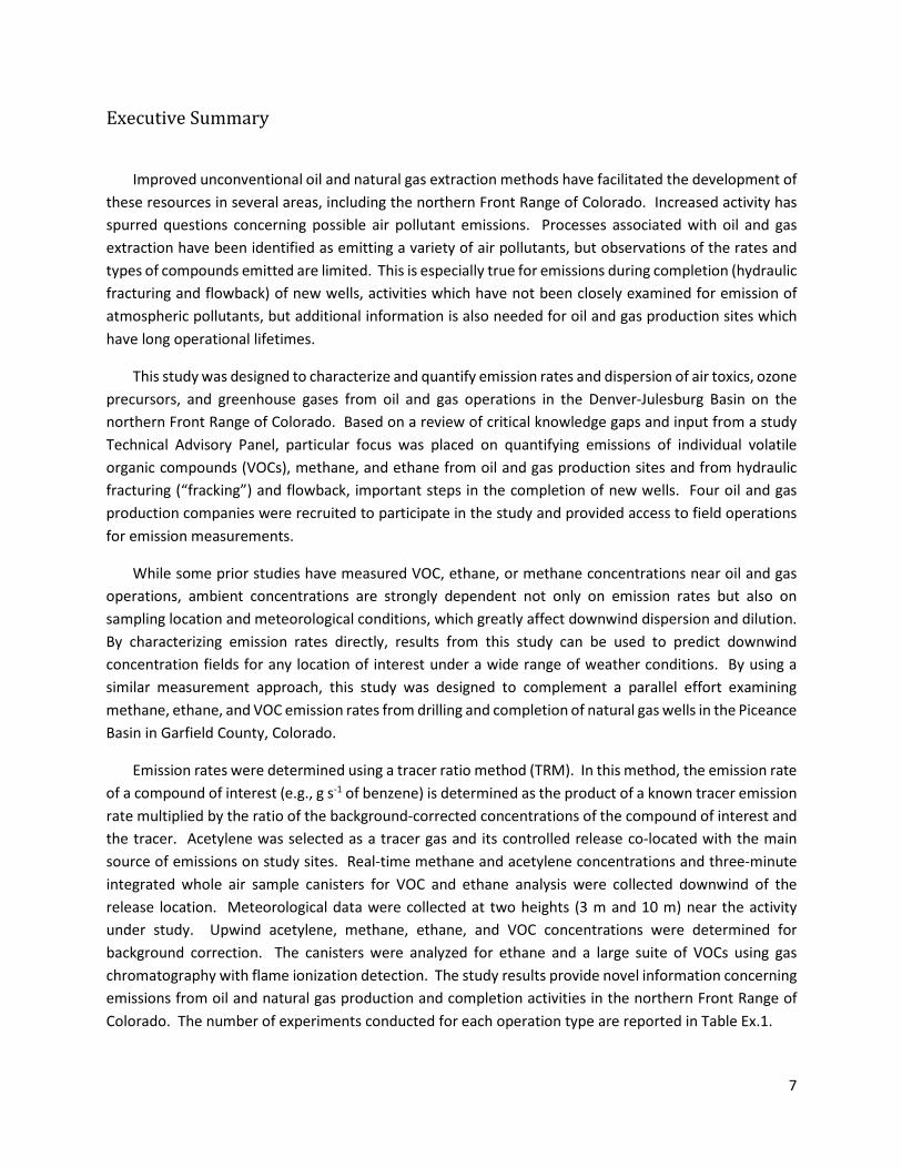
Improved unconventional oil and natural gas extraction methods have facilitated the development of these resources in several areas, including the northern Front Range of Colorado. Increased activity has spurred questions concerning possible air pollutant emissions. Processes associated with oil and gas extraction have been identified as emitting a variety of air pollutants, but observations of the rates and types of compounds emitted are limited. This is especially true for emissions during completion (hydraulic fracturing and flowback) of new wells, activities which have not been closely examined for emission of atmospheric pollutants, but additional information is also needed for oil and gas production sites which have long operational lifetimes.
This study was designed to characterize and quantify emission rates and dispersion of air toxics, ozone precursors, and greenhouse gases from oil and gas operations in the Denver-Julesburg Basin on the northern Front Range of Colorado. Based on a review of critical knowledge gaps and input from a study Technical Advisory Panel, particular focus was placed on quantifying emissions of individual volatile organic compounds (VOCs), methane, and ethane from oil and gas production sites and from hydraulic fracturing (“fracking”) and flowback, important steps in the completion of new wells. Four oil and gas production companies were recruited to participate in the study and provided access to field operations for emission measurements.
While some prior studies have measured VOC, ethane, or methane concentrations near oil and gas operations, ambient concentrations are strongly dependent not only on emission rates but also on sampling location and meteorological conditions, which greatly affect downwind dispersion and dilution. By characterizing emission rates directly, results from this study can be used to predict downwind concentration fields for any location of interest under a wide range of weather conditions. By using a similar measurement approach, this study was designed to complement a parallel effort examining methane, ethane, and VOC emission rates from drilling and completion of natural gas wells in the Piceance Basin in Garfield County, Colorado.
Emission rates were determined using a tracer ratio method (TRM). In this method, the emission rate of a compound of interest (e.g., g s-1 of benzene) is determined as the product of a known tracer emission rate multiplied by the ratio of the background-corrected concentrations of the compound of interest and the tracer. Acetylene was selected as a tracer gas and its controlled release co-located with the main source of emissions on study sites. Real-time methane and acetylene concentrations and three-minute integrated whole air sample canisters for VOC and ethane analysis were collected downwind of the release location. Meteorological data were collected at two heights (3 m and 10 m) near the activity under study. Upwind acetylene, methane, ethane, and VOC concentrations were determined for background correction. The canisters were analyzed for ethane and a large suite of VOCs using gas chromatography with flame ionization detection. The study results provide novel information concerning emissions from oil and natural gas production and completion activities in the northern Front Range of Colorado. The number of experiments conducted for each operation type are reported in Table Ex.1.

8
Table Ex.1. Number of experiments conducted during this study for different types of operations.
Type of Operation Number of experiments
Fracking 3 Flowback 3 Production 10 Production and Flowback 1 Liquids Load Out 1
Overall, 18 emission experiments were conducted from 2014-2016. Several sets of canisters were collected at different times during each experiment, in addition to upwind background samples. Using the TRM, each canister in the plume provides an independent measure of ethane and VOC emission rates. Ethane and 47 VOCs are reported for each canister, along with real-time methane and acetylene data collected during each experiment. Using the TRM, the emission rates of methane, ethane, and individual VOCs are calculated and reported. Table Ex.2 shows median emission rates of methane, ethane, and several key VOCs for each major operation type. Methane, ethane, and propane were the most abundant constituents in measured emissions. Generally, higher rates of VOC, ethane, and methane emissions were observed during flowback operations, although a wide range of emissions was observed for each type of activity studied. Methane emission rates were examined as a percentage of produced natural gas at the diverse array of production sites included in the experiment. These included large and small sites (between 1 and 18 horizontal and/or vertical wells) with a variety of different separation schemes. A positive relationship was observed with gas production rate; median and mean methane emissions measured across all production sites were 0.23% and 0.37%, respectively, with the 95th percentile of emissions at 1.03%.
Table Ex.2. Median values of methane and select VOC emission rates from measurements during different operation types.
Production Median (g s-1)
Fracking Median (g s-1)
Flowback Median (g s-1)
Methane 0.60 0.051 2.76 Ethane 0.10 0.0026 1.09 Propane 0.088 0.00049 0.75 i-Pentane 0.018 0.00073 0.30 n-Pentane 0.017 0.00028 0.39 Benzene 0.0013 0.0022 0.069 Toluene 0.0011 0.0056 0.21 Ethylbenzene 0.00022 0.00084 0.0019 m+p-Xylene 0.000108 0.0040 0.24
The emission rates and field observations were used to conduct air dispersion simulations (using EPA’s AERMOD model) to: (1) evaluate AERMOD’s accuracy in predicting observed, near-field dispersion of ethane and VOCs in the Colorado Front Range and (2) predict concentration fields, as a function of
9
emission rate, for dispersion of benzene under a range of local meteorological conditions at a site with terrain similar to that observed in the Front Range of Colorado. While not perfectly designed for prediction of the short-term concentration fields measured in this study, AERMOD did a reasonable job predicting the observed extent of dispersion across several field experiments. Moreover, emission rate ranges determined by activity type in this study can be used in a wide range of future simulations with AERMOD or other models to simulate downwind concentration fields relevant to understanding potential local health and air quality impacts associated with oil and gas well completion and production activities on the northern Front Range.
The data collected during this study are available for public access at: (http://www.colorado.gov/airquality/tech_doc_repository.aspx#special_studies). A more detailed and technical discussion of the study and its findings follows this summary.

10
List of Participants Funding Sources: Colorado Department of Public Health and Environment City of Fort Collins, Colorado
Industry participants: Encana Corporation Anadarko Petroleum Company PDC Energy, Inc. Noble Energy, Inc. Technical Advisory Panel (listed alphabetically): Ms. Cassie Archuleta, City of Fort Collins Dr. Ramon Alvarez, EDF Mr. Adam Berig, Encana Corporation Mr. Trevor Jiricek, Weld County Department of Public Health and Environment Ms. Pam Milmoe, Boulder County Air Quality/Business Sustainability Program Dr. Gabriele Pfister, National Center for Atmospheric Research Mr. Gordon Pierce, TAP Chair, APCD/CDPHE Mr. Chad Schlichtemeier, Anadarko Petroleum Corporation Dr. Barkley Sive, National Park Service Mr. Peter Stevenson, DCP Midstream Mr. Brian Taylor, Noble Energy Dr. Gail Tonnesen, US EPA Project Research Team: Colorado State University Air Resource Specialists Prof. Jeffrey L. Collett, Jr (PI) Mr. Mark Tigges Prof. Jay Ham (co-PI) Mr. Bryan Bibeau Prof. Jeffrey Pierce Mr. Christian Kirk Dr. Arsineh Hecobian Mr. Howard Gebhart Dr. Andrea Clements Mr. Douglas Ingersoll Ms. Kira Shonkwiler Dr. Yong Zhou Dr. Yuri Desyaterik Mr. Landan MacDonald Mr. Bradley Wells Ms. Noel Hilliard

11
1. Introduction 1.1. Background and Study Objectives The Denver-Julesburg Basin (D-J Basin) extends over an area of more than 70,000 square miles (mi2)
in eastern Colorado, southeastern Wyoming, and southwestern Nebraska as shown in Figure 1.1. The first recorded commercially producing well from this basin was the McKenzie Well in 1902 (History Colorado, 2016). The Wattenberg field has been a center for unconventional oil and gas extraction (COGCC, 2007).
Figure 1.1. Map of Colorado and surrounding states, showing the Denver Julesburg Basin in light green, and the Wattenberg formation in red.
Approximately 87% of Colorado’s active wells (~54000) are located in 6 counties, with about 42% located in Weld County (COGCC, 2016). More than half of the permits requested from the Colorado Oil and Gas Conservation Commission (COGCC) in 2015 and 2016 were for Weld County. Total annual natural gas production has been increasing in Colorado since 1995 such that the natural gas production levels per day for 2015 were three times higher than those in 1995 (COGCC, 2016). A similar trend was observed for oil production in Colorado, with a four-fold increase from 1995 to 2015. Figure 1.2 depicts oil and gas well locations in NE Colorado. A large concentration of wells can be seen in Weld County under which most of the Wattenberg formation is located.

12
Figure 1.2. Map of northern Front Range of Colorado with county boundaries. The dots indicate locations of wells in this area. The Wattenberg field is outlined in red.
The increase in oil and gas production in the D-J basin is partly due to technological improvements that allow access to resources in formations that were previously unfeasible or uneconomical to tap. Unconventional oil and gas extraction methods such as horizontal drilling and hydraulic fracturing are frequently utilized to extract natural gas from low-permeability formations like tight sandstone and shale. The typical vertical depth of a well is between 5000-9000 feet; after reaching a location near the shale/sandstone formation, a directional drill can be used for horizontal drilling for 5000 feet or more. Multiple horizontal wells accessing the same or other close-by formations can be drilled from one pad. The drilling phase usually takes 4-10 days per well. After drilling is complete, hydraulic fracturing is used to inject water, sand, and chemicals into the well at high pressures. The fluid is used to open previously made fractures and connect them to create better pathways for more efficient flow of oil and gas to the surface. Hydraulic fracturing is applied to each well in sections and, at completion, each section is closed using a cement plug. The hydraulic fracture phase of each well can span a period of 2-4 days. After the entire well is fracked, the plugs are drilled out to enable the flow of fracking fluid, produced water, oil, and natural gas up the well. This phase of well completion is known as flowback. The flowback water has typically been stored on the pad and later transported for underground (well injection) storage or recycling and re-use in future hydraulic fracturing activities. Traditionally, an initial flowback period can last for 7-12 days per well, after which the fluid flow is reduced and the oil and natural gas can be directed to storage or processed and directed to production sites and sales pipelines. The length of each stage (drilling, hydraulic fracturing, and flowback) can vary by site and is dependent on the number of wells planned for the pad. Some operators are now sending well flowback directly to permanent production equipment with increased frequency of flowback liquid load out.
Colorado State University’s (CSU’s) Dr. Jeffrey Collett and Dr. Jay Ham proposed a study to characterize emissions from oil and gas development and production activities on the northern Front

13
Range. As part of the study, a Technical Advisory Panel (TAP) was assembled. The TAP consisted of individuals with technical expertise concerning air pollution and/or air emissions associated with oil and gas development from a wide range of stakeholders, including government agencies (federal, state, and local), non-governmental organizations, research institutes, and industry. Following a review of critical gaps in knowledge concerning air emissions and with input from the TAP, measurement priorities were established. Chief among these priorities were emissions from oil and gas production sites and from two stages of well completion: hydraulic fracturing and flowback. As part of this prioritization, consideration was given to planned measurements in a parallel emissions study examining natural gas well drilling and completions in the Piceance Basin in Garfield County, Colorado. Drilling emissions, for example, received a lower priority in the North Front Range study because they were included in the Garfield County study (CSU, 2016) while production emissions were a priority here in part due to the fact that they were not examined in Garfield County. Production emissions were also given high priority due to the much longer lifetime of this activity type (decades) relative to drilling and completion activities (days to weeks).
A variety of volatile organic compounds can be released to the atmosphere from oil and gas development and production. The primary focus of the study is to quantify emissions of air toxics, ozone precursors, and greenhouse gases from oil and gas production and from fracking and flowback activities. Specifically, the study examined emission rates of methane, ethane, and a wide range of individual volatile organic compounds (VOCs) and their near-field dispersion. Primary funding for the study came from the Colorado Department of Public Health and Environment (CDPHE), with additional funding contributed by the City of Fort Collins.
The approach used for the field measurements, very similar to the approach used in the Garfield County study to ensure comparability of measured emissions, is described in Section 2. Briefly, the CSU team worked with industry partners to identify sites with hydraulic fracturing, flowback, or production activities available for characterization. Site selection criteria also included local terrain and accessibility for downwind measurements. The Tracer Ratio Method (TRM), described by Lamb et al. (1995), was used to quantify emission rates (ERs) of methane, ethane, and VOCs from natural gas well development and production activities. In this approach a conservative tracer is co-located with the source of interest and emitted at a controlled rate. The rate of emission of a compound of interest (e.g., g s-1 of benzene) is determined as the product of the tracer emission rate multiplied by the ratio of the background-corrected concentrations of the compound of interest and the tracer. Through this technique, the complex dispersion and dilution that occurs during turbulent transport from the emissions point to the measurement point is directly accounted for by the dilution of the tracer. A tracer release system (Section 2.2.1) was stationed on the pad and co-located with the major identified emission source. A tracer gas (acetylene) was emitted at a known flow rate. CSU’s mobile plume tracker, equipped with an analyzer (Picarro Cavity Ringdown System) for the real-time measurement of methane and acetylene (Section 2.2.2), was deployed downwind to detect the tracer gas and locate the plume. When a plume was identified, evacuated Silonite® coated stainless steel canisters were remotely triggered (Section 2.2.4) to collect whole air samples for 3 minutes. The sampled canisters were transported to CSU for subsequent ethane and VOC analysis using Gas Chromatography with Flame Ionization Detection (GC-FID) (Section 2.2.5). Measurements were also made upwind of the study site to determine background concentrations.

14
The real-time methane and acetylene data (Section 2.3.1) and the canister ethane and VOC data (Section 2.3.2) were analyzed to determine the ERs of methane, ethane, and VOCs from each study site and activity. Use of the background methane, ethane, and VOC data in the ER calculations ensured that the identified emissions were limited to those associated with targeted activity at the study site. Emission results are presented in Sections 3.1, 3.2, and 3.3.
The EPA dispersion model (AERMOD) was used to model the dispersion of emissions at each study site in order to compare predicted concentration fields with those observed, providing an assessment of the accuracy of the model predictions. AERMOD was also run over a longer period at a typical site with terrain characteristic of sites visited as part of this study to simulate how near-field concentrations of compounds of interest are predicted to vary over a range of typical meteorological conditions. AERMOD model parameters are described in Section 2.3.3 and the results from the modeling analyses are presented in Section 3.4.
1.2. Overview of Sample Collection 1.2.1. Site Selection Members of the CSU research team worked with the study’s four industry partners to identify
locations where hydraulic fracturing or flowback activities were planned. Industry partners also provided access to oil and gas production sites; in selecting production sites, CSU selected operations with differing generations of production and emissions control equipment (e.g., number of separation stages). Once potential sites were identified, local terrain and meteorological conditions typical of the pad were investigated by the CSU research team and the accessibility of the area surrounding the site was examined. The CSU team visited the sites prior to measurements to evaluate the feasibility of sampling based on location and downwind terrain access. The dates of measurements were announced to companies with 24 hrs. or less, advance notice. In some cases the CSU team sought and received on-the-spot permission to conduct measurements immediately at sites not included on the original site access list.
Whenever possible, sites were selected where only a single operation was underway: fracking, flowback, or production. One site was included where conventional flowback operations were not conducted. Flowback fluids in this operation were sent directly to permanent production equipment; emissions from this experiment are grouped with other production site emissions in most analyses in this report. During a visit to one production site the CSU measurement team was made aware that liquid flowing back from recently completed wells was being loaded to a truck. This experiment has been categorized as Liquids Load Out. This site has measurements for when no liquids Load Out was taking place (Production activity only; Experiment #7) and when Liquids Load Out and Production activities were present (Experiment #8).
1.2.2. Equipment Setup For each emission experiment, a meteorological station (Section 2.2.3), a mobile plume tracker (a
Hybrid Chevy Tahoe, see Section 2.2.2), the tracer release system (2.2.1), and ethane and VOC canister sampling systems (2.2.4) were positioned on and around the pad, with the tracer release system being co-located with the primary point of emissions for a particular activity. The meteorological station was

15
usually positioned upwind of the pad. Canisters were positioned both upwind (for background sample collection) and downwind. Figure 1.3 provides an overview of the equipment setup at a typical site.
Figure 1.3. Overview of equipment setup at a typical site, adapted from MacDonald (2015).
1.2.3. Sampling Overview The tracer release system was set up on the pad and, when ready, the tracer gas was released when
meteorological conditions stabilized and appeared favorable for a successful experiment. The plume tracker vehicle was driven downwind of the pad to locate the plume. Once the plume was located, the plume tracker vehicle would stop and three evacuated canisters would be deployed (two near the vehicle at different heights and one closer/farther from the pad, on a tripod). Using remote triggering systems, the canisters would be triggered simultaneously to collect ambient air for 3 minutes. At the conclusion of the sample collection, new canisters would be attached and ready for the next sample collection period. Typically, 4-6 sets of 3 canisters were collected at each site. Canisters were collected at a range of distances (38-721 meters) which depended on site access and meteorological conditions. Table 1.1 presents information on the site operation type, number of canisters and sets of canisters collected from each site. Variations in the number of canisters collected are due to changes made because of meteorological conditions, changes in site operations, or terrain conditions downwind of the pad.
Trucks, generators, or pumps
Liquid storage containers
Met Station
Natural gas storage containers
Well heads

16
Table 1.1. Number of experiments and information on operation types, number, and sets of canisters collected.
Experiment # Type of Operation
Number of Canisters (including background)
Sets of Canisters (number of measurement periods)
1 Production 11 5 2 Fracking 11 4 3 Fracking 15 5 4 Production 15 5 5 Production 15 5 6 Production 15 5 7 Production (with Flowback) 16 6 8 Liquids Load Out 6 2 9 Flowback 14 5 10 Flowback 12 4 11 Fracking 17 8 12 Flowback 13 6 13 Production 15 5 14 Production 21 7 15 Production 13 4 16 Production 16 5 17 Production 12 4 18 Production 12 4
For each site visited, at least one canister was collected immediately upwind of the site to represent
background concentrations of ethane and VOCs at that site. This background correction ensures that reported emissions reflect only those emitted from the well pad being studied and do not include emissions from other nearby or regional sources. Usually, acetylene was released at the time of background collection and the mobile plume tracker was used to ensure that no above-background acetylene was observed during the collection of the background canister. Background methane concentrations were also determined from the real-time measurements aboard the plume tracker vehicle made during periods outside the plume emitted from the site, as represented by acetylene tracer concentrations, also measured in real-time.
2. Measurement Methods 2.1. Tracer Ratio Method The TRM is a straightforward technique that requires access to the emission source and involves the
release of a passive tracer gas co-located with the source of emissions. The known ER of the tracer gas is multiplied by the ratio of the downwind concentrations of the emitted gas to the tracer gas (both in excess of background) to determine the ER of the gas of interest. The TRM has been used as a technique for estimating the ERs of gases from a variety of sources (e.g., Lamb et al., 1986; Lassey et al., 1997; Rumburg et al., 2008; Scholtens et al., 2004). In this study, acetylene (also known as ethyne, C2H2) was used as the tracer gas. Acetylene was chosen because of its chemical stability, relatively long lifetime in the

17
atmosphere (~2 weeks), ease of detection at high time resolution and low concentrations, and absence as a major emission of oil and gas operations.
The following equation was used to calculate the ERs of methane, ethane, and VOCs,
𝑄𝑄𝑉𝑉𝑉𝑉𝑉𝑉 = 𝑄𝑄𝑉𝑉2𝐻𝐻2 ∗ [𝑉𝑉𝑉𝑉𝑉𝑉][𝑉𝑉2𝐻𝐻2]
where, 𝑄𝑄𝑉𝑉𝑉𝑉𝑉𝑉 is the ER of the desired species, 𝑄𝑄𝑉𝑉2𝐻𝐻2 is the (known) release rate of acetylene, and [𝑉𝑉𝑉𝑉𝑉𝑉] and [𝑉𝑉2𝐻𝐻2] are the background-corrected concentrations of the emitted gas (methane, ethane, or VOC) and the tracer gas (acetylene), respectively. The concentrations can be integrated over space and/or time depending on the type of analysis performed. In this study, both the instantaneous and time integrated concentrations were used during data analysis. The instantaneous concentrations were used for estimating ERs of methane and the time integrated concentrations were used to report the ERs of ethane and VOCs. The basic assumptions of TRM are:
• The ER of the tracer is accurately known. • The concentrations measured downwind are accurate. • The two gaseous species disperse in a similar manner. • The tracer is co-located with the emission source being characterized. • Neither the tracer, nor the target VOC (or methane or ethane) are altered by deposition or
chemical reaction between the release and detection points.
In order to evaluate the accuracy of this method, several controlled release experiments were conducted where acetylene and methane were collocated and released at known ERs. TRM was used to estimate the ER of methane and the results were compared with the known values to determine the method uncertainty. Wells (2015) provides a detailed description of these experiments. The TRM method uncertainty in the controlled release experiments (Wells et al., 2016) was characterized by an accuracy (mean bias) of +22.6% and a precision of ±16.7% (relative standard deviation). As shown in Table 2.1, the precision reported here is similar to values reported from other studies. The accuracy and precision of the TRM method are considered more than acceptable, particularly given the large variability in actual emission rates observed in study field experiments. The precision of the TRM was also evaluated for individual VOC and ethane emission rates using replicate canister measurements collected during the field study; precision varied between approximately 1 and 55% (pooled relative standard deviation) for individual VOCs and ethane, with most values less than 20%.
Table 2.1. TRM method precision reported by various studies.
Study Precision (%) Lamb et al. (1995) ±15 Kaharabata & Schuepp (2000) ±30 Galle et al. (2001) ±15 to ±30 Scholtens et al. (2004) -25 to +43 Mǿnster et al. (2014) ±5 This study (Wells et al., 2016) ±17

18
2.2. Measurement Techniques 2.2.1. Tracer Release System
A tracer release system was designed to ensure consistent, quantified, and safe release of the acetylene near the pre-identified main source of emissions on a study site. This system consisted of three acetylene cylinders that were connected in parallel to a regulator to ensure pressure equilibration in each cylinder and to prevent the release of liquid acetone from the acetylene tank into the regulator and the lines. The regulator controlled the pressure of acetylene as it entered the attached Bev-A-Line IV non-reactive plastic tubing. An Alicat M-Series Mass Flow Controller (MFC) was used to regulate the acetylene flow, which allowed the appropriate mass flux of gas to enter a mixing chamber. The acetylene gas was diluted with ambient air to keep the concentrations below the Lower Explosive Limit (LEL). The diluted tracer gas was then transported via an accordion hose to a 6 m-long perforated manifold, held ~4m above ground on aluminum tripods, for release. Generally, release flow rates of at least 10 standard liters per minute (slpm) were utilized to ensure the concentrations observed downwind were adequately above background levels. A Campbell Scientific CR850 Data Logger was used to record the temperature, pressure, and acetylene mass flow rate as a function of time at 1 Hz. Figure 2.1 is a diagram of this system and Figure 2.2 is a photo of the system as deployed in the field.
Figure 2.1. Diagram of the tracer release control system and C2H2 cylinders adapted from Wells et al. (2016). Acetylene cylinders are connected to a mass flow controller (MFC) and directed to a mixing box with a lower explosive limit (LEL) detector. The acetylene is then directed to a perforated manifold for release to the atmosphere as presented in Figure 2.2.

19
Figure 2.2. Photo of the tracer release system as deployed in the field. The C2H2 cylinders and the tracer release control system are presented in Figure 2.1.
2.2.2. Mobile Plume Tracker Downwind of the tracer release system, a mobile plume tracker was deployed to measure the
concentration of acetylene (the tracer gas) and methane. This system consisted of a Chevrolet Tahoe hybrid sport utility vehicle that housed a Picarro G2203 analyzer and A0931 mobile measurement kit that collected data on the concentrations of methane and acetylene using cavity ring-down spectroscopy (CRDS). The instrument inlet was located at a height of 3 m in the front of the SUV and was connected to the analyzer using ~4.5 m Teflon® tubing which directed ambient air into the Picarro system at 5 L min-1. Adjacent to the Picarro inlet was a Global Positioning System (GPS) and an All-In-One meteorological sensor for wind speed and wind direction measurements. The data from the analyzer were displayed inside the plume tracker vehicle in real-time. Table 2.2 summarizes the measurement capabilities of this system. Table 2.2. Instrument description and measurement capabilities of the mobile plume tracker.
Instrument Type Model Manufacturer Measurement Interval CRDS methane and acetylene analyzer G2203 Picarro 3Hz
Mobile computer for analyzers A0931 Picarro 3Hz
GPS A21 Hemisphere GNSS 3Hz Wind speed and direction 102779-A1-C1-D0 Climatronics 3Hz
20
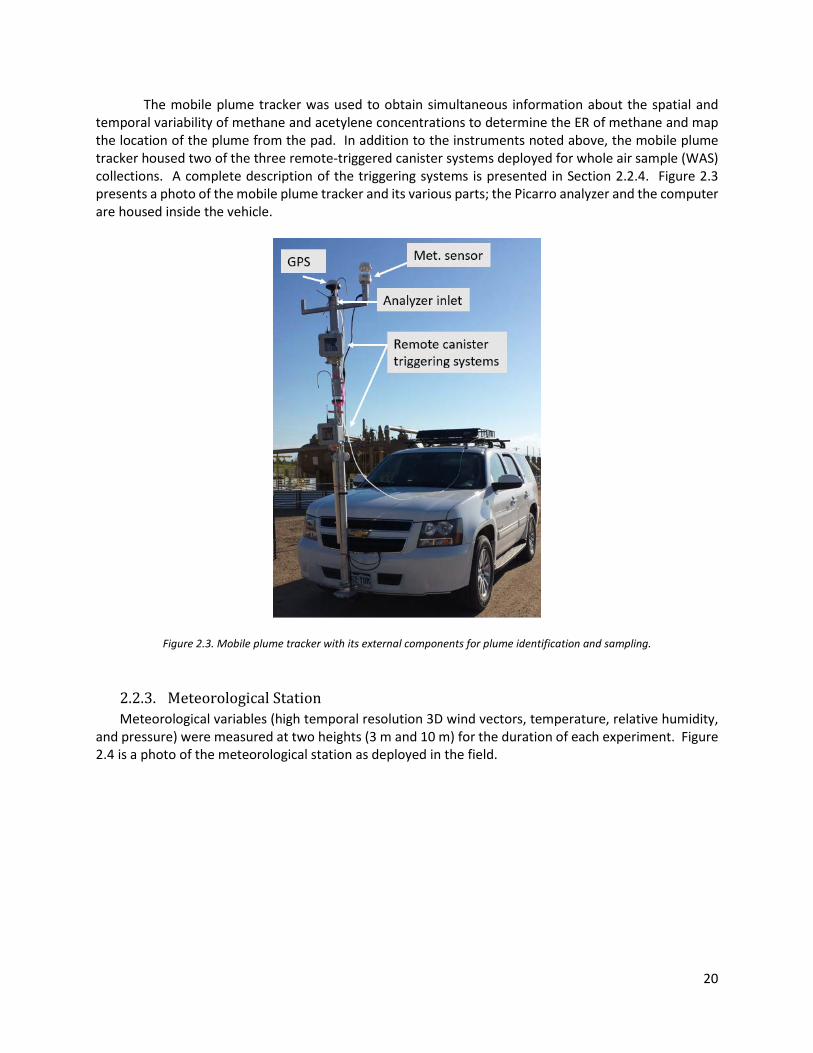
The mobile plume tracker was used to obtain simultaneous information about the spatial and temporal variability of methane and acetylene concentrations to determine the ER of methane and map the location of the plume from the pad. In addition to the instruments noted above, the mobile plume tracker housed two of the three remote-triggered canister systems deployed for whole air sample (WAS) collections. A complete description of the triggering systems is presented in Section 2.2.4. Figure 2.3 presents a photo of the mobile plume tracker and its various parts; the Picarro analyzer and the computer are housed inside the vehicle.
Figure 2.3. Mobile plume tracker with its external components for plume identification and sampling.
2.2.3. Meteorological Station Meteorological variables (high temporal resolution 3D wind vectors, temperature, relative humidity,
and pressure) were measured at two heights (3 m and 10 m) for the duration of each experiment. Figure 2.4 is a photo of the meteorological station as deployed in the field.

21
Figure 2.4. Picture of the meteorological station used for measurements during this study.
A summary of the meteorological instruments that were used and the type of data collected are given
in Table 2.3. Table 2.3. Instruments used for the collection of meteorological data.
Instrument Type Model Manufacturer Measurements
Sonic Anemometer WindMaster Gill 3D wind vectors, temperature, and water vapor concentrations
Weather Station All-In-One Climatronics 2D wind vectors, temperature, pressure, and relative humidity
Wind Monitor 05103 R. M. Young Wind direction and speed Data Logger CR1000 Campbell Scientific Data acquisition and storage
2.2.4. Canister Triggering System Evacuated 1.4 L Silonite®-coated stainless steel canisters (Entech Instruments, Simi Valley, CA)
coupled with remote triggering systems (Air Resource Specialists, Fort Collins, CO), were used for the collection of whole air samples. Typically, three canisters were deployed for each sample period: two were positioned adjacent to the mobile plume tracker at different heights and a third canister was positioned either further downwind or upwind of the mobile plume tracker based on the terrain and general layout of the site. The location of the triggering systems with respect to the mobile plume tracker is shown in Figure 2.3. The third canister was positioned on a tripod about 2 m above ground. Figure 2.5 is a photo of the third canister triggering system and its components.

22
Figure 2.5. Photo of the third canister triggering system and its components, deployed on a tripod.
The triggering systems were outfitted with an Arduino UNO microcontroller controlled solenoid valve that was opened for a total of 180 seconds to allow ambient air to be sampled into the previously evacuated canister for later analysis. A pressure sensor, GPS, and temperature sensor were placed within the fiberglass enclosure of the triggering system. A detailed list of the components is included in Table 2.4. A custom LabVIEW interface remotely activated the triggering systems to open simultaneously using a portable netbook computer. Table 2.4. List of components from the canister remote triggering system (Air Resource Specialists, Fort Collins, CO).
Component Model Manufacturer Microcontroller UNO Arduino GPS PMB-688 Polstar Temperature Sensor LM35 Texas Instruments Wireless Modem XBee-PRO 900HP Digi Pressure Sensor OEM 0-15 PSIA Honeywell Solenoid Valve S311PF15V2AD5L GC
2.2.5. Canister VOC and Ethane Measurement System
VOCs in this report are defined as compounds containing carbon, excluding carbon monoxide, carbon dioxide, carbonic acid, metallic carbides, carbonate and ammonium carbonate, methane, and ethane. A list of the VOCs (and ethane) measured and reported in this study is presented in Table B.1 of Appendix B.
23
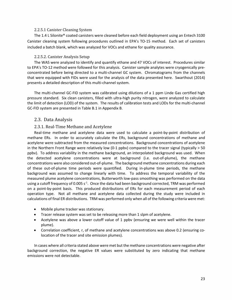
2.2.5.1 Canister Cleaning System The 1.4 L Silonite® coated canisters were cleaned before each field deployment using an Entech 3100
Canister cleaning system following procedures outlined in EPA’s TO-15 method. Each set of canisters included a batch blank, which was analyzed for VOCs and ethane for quality assurance.
2.2.5.2. Canister Analysis Setup The WAS were analyzed to identify and quantify ethane and 47 VOCs of interest. Procedures similar
to EPA’s TO-12 method were followed for this analysis. Canister sample analytes were cryogenically pre-concentrated before being directed to a multi-channel GC system. Chromatograms from the channels that were equipped with FIDs were used for the analysis of the data presented here. Swarthout (2014) presents a detailed description of this multi-channel system.
The multi-channel GC-FID system was calibrated using dilutions of a 1 ppm Linde Gas certified high pressure standard. Six clean canisters, filled with ultra-high purity nitrogen, were analyzed to calculate the limit of detection (LOD) of the system. The results of calibration tests and LODs for the multi-channel GC-FID system are presented in Table B.1 in Appendix B.
2.3. Data Analysis 2.3.1. Real-Time Methane and Acetylene Real-time methane and acetylene data were used to calculate a point-by-point distribution of
methane ERs. In order to accurately calculate the ERs, background concentrations of methane and acetylene were subtracted from the measured concentrations. Background concentrations of acetylene in the Northern Front Range were relatively low (0-1 ppbv) compared to the tracer signal (typically > 50 ppbv). To address variability in the methane background, an interpolated background was used. When the detected acetylene concentrations were at background (i.e. out-of-plume), the methane concentrations were also considered out-of-plume. The background methane concentrations during each of these out-of-plume time periods were quantified. During in-plume time periods, the methane background was assumed to change linearly with time. To address the temporal variability of the measured plume acetylene concentrations, Butterworth low-pass smoothing was performed on the data using a cutoff frequency of 0.005 s-1. Once the data had been background corrected, TRM was performed on a point-by-point basis. This produced distributions of ERs for each measurement period of each operation type. Not all methane and acetylene data collected during the study were included in calculations of final ER distributions. TRM was performed only when all of the following criteria were met:
• Mobile plume tracker was stationary. • Tracer release system was set to be releasing more than 1 slpm of acetylene. • Acetylene was above a lower cutoff value of 1 ppbv (ensuring we were well within the tracer
plume). • Correlation coefficient, r, of methane and acetylene concentrations was above 0.2 (ensuring co-
location of the tracer and site emission plumes). In cases where all criteria stated above were met but the methane concentrations were negative after
background correction, the negative ER values were substituted by zero indicating that methane emissions were not detectable.

24
2.3.2. Canister VOCs and Ethane The acetylene concentrations within canisters were evaluated to assess whether a canister was
collected inside or outside of the emission plume coming off the study site. Canister samples – except those collected to represent site background concentrations - were discarded if the acetylene concentration was less than 2.2 ppbv. This acetylene cutoff was selected by adding the average (1.09 ppbv) and one standard deviation (1.10 ppbv) of the C2H2 background concentrations for all canisters collected during the study.
The ranges of background concentrations for ethane and all VOCs from background canisters collected throughout the study are presented in Appendix A. In some instances concentrations were below the multi-channel GC-FID limit of detection (LOD), in which case the measured value was replaced with LOD/2 for the corresponding VOC or ethane. The LODs for the multi-channel GC-FID system for each VOC and ethane are presented in Appendix B. After the substitution, canister VOC and ethane data were background corrected. The background correction involved subtracting the concentrations measured from the background canister(s) deployed upwind of the emission location from the VOC and ethane values in the sampled canister. In cases where the background was equal to or higher than the measured concentration of a VOC or ethane, the calculated value was replaced with LOD/2. After processing the concentrations of the VOCs and ethane found in the downwind canister samples, the ERs of the VOCs and ethane were calculated using the TRM method as described in Section 2.1.
2.3.3 Dispersion Modeling Using AERMOD AERMOD is an atmospheric dispersion model approved by USEPA and frequently used to characterize
the impact of a new emission source (Cimorelli et al., 2004). It has the ability to incorporate complex terrain, feature multiple sources and receptors, and determine downwind concentration fields within 50 km of the source. AERMOD disperses plumes using hourly averaged meteorology. It assumes the plume to be Gaussian within both the stable boundary layer (SBL) and in the convective boundary layer (CBL). AERMOD was used in this study for two analyses: (1) to replicate the time/location of each field measurement using a combination of field meteorological measurements and CDPHE data to compare AERMOD predicted concentration fields with ambient concentration measurements, and (2) to simulate a distribution of expected benzene concentrations, for an assumed emission rate, for a site location typical of those visited as part of this study, using archived meteorological fields, with model run simulations which were one year long. The former application is intended to evaluate the ability of AERMOD to accurately predict air pollutant dispersion under conditions observed during this study, while the latter application is intended to illustrate AERMOD capabilities for future prediction of air pollutant concentration fields associated with activity emission rates determined in this study. Benzene is chosen for this example because it is an air toxic for which near-source concentration fields are of interest.
The surface and sounding meteorological data used in the analysis presented here were obtained
from on-site measurements as described above and from CDPHE for two different stations: Fort St. Vrain (40.254°, -104.872°) for 2009 and Rawhide (40.854°, -105.038°) for 2006.
3. Results 3.1. Methane ERs Approximately 74,500 total methane emission measurements were made across all experiments,
representing a total in-plume measurement time of 6.9 hrs. The overall methane ER distribution dataset spans over 5 orders of magnitude, clearly indicating the large variability in methane emissions observed during the study and for different operation types. The majority of methane emission rates fall between

25
approximately 0.06 and 2.6 g s-1. Methane emissions were not detected in approximately 12% of all measurement periods.
The methane ER data were classified by operation type as outlined in Table 1.1. Figure 3.1 shows separate distributions of methane ERs for each type of operation including fracking, flowback, production, and liquids load out in the left panel and the median and range of the values for each operation in the right panel. The median methane ER was highest for the liquids load out activity (4.8 g s-1; 1 experiment), followed by flowback (2.8 g s-1; 3 experiments), production (0.60 g s-1; 11 experiments), and fracking (0.05 g s-1; 3 experiments). A wide range of methane ERs was observed for each of these activities with some overlap between the distributions observed for different operations. Table 3.1 provides a statistical summary of the results in Figure 3.1. The methane ER distributions for individual experiments are plotted separately in Appendix C.
Figure 3.1. Methane ER distributions by operation type. Left Panel: Normalized frequency distributions of methane ERs. T indicates the total amount of time when data were successfully collected across all experiments for each operation type at 3 Hz. Only measurement periods meeting the quality control criteria outlined in Section 2.3.1 are included. Right Panel: Box and whisker plot of the methane ERs. The blue line indicates the median; the top and bottom of the box and the top and bottom whiskers represent the 75th and 25th and the 95thand 5th percentiles, respectively. The circles represent all the data above or below the 99th and 1st percentiles.
0.0
0.2
0.4
0.6
0.8
1.E-05 1.E-03 1.E-01 1.E+01 1.E+03
Nor
mal
ized
Freq
uenc
y
Methane Emission Rate (gs-1)
Fracking T=0.65hr~18% below detection
Production T=4.88hr~14% below detection
Flowback T=1.32hr~6% below detection
Liq. Load Out T=0.07hr~6% below detection

26
Table 3.1. ER distributions of methane calculated using the TRM. The data are separated into their respective operation types.
Operation Type # of Experiments
T (hrs)
Mean (g s-1)
Median (g s-1)
25th %ile (g s-1)
75th %ile (g s-1)
Fracking 3 0.65 0.29 0.051 0.0031 0.12 Flowback 3 1.32 7.6 2.8 0.86 7.3 Production 11 4.88 5.7 0.60 0.054 2.0 Liquids load out 1 0.07 13.0 4.8 0.40 13.9
The production emission rates of methane reported here encompass a wide range of sites with different total production rates, fed by different numbers of horizontal and/or vertical wells, and with different types of emission control equipment. For example, the number of wells per site ranged from 1 to 18 and the number of condensate tanks from 0 to 27, while the stages of separation also differed across sites. Details about production operations at each site, provided by the operators, are presented in Table E.1 in Appendix E.
The fracking and flowback methane emissions observed here are lower than those recently reported for a similar study of completion emissions in the Piceance Basin in Garfield County (CSU, 2016). The median methane ERs reported for fracking (5 experiments) and flowback (6 experiments) in the Piceance Basin study were 2.8 g s-1 and 40 g s-1, respectively.
3.2. Normalized Methane Production Site ERs Given the large variability in production rates, numbers of wells, well type, and separation schemes
utilized at different production sites, it is not surprising that methane ERs might vary across production sites. It is also important to recognize that methane ERs from a given production site are expected to decrease over time as wells age and overall production at the site declines. By utilizing information about production operations at individual sites provided by participating operators (see Table E.1), we can examine whether ERs vary as a function of overall production rate or other key parameters. The left panel of Figure 3.2 presents the median methane ERs for production experiments vs. the average daily gas production rates (for the month of the measurement) at each site. Production sites are further segregated by the types of wells (horizontal, vertical, or both), the number of wells feeding the production site at the time of measurement, and the stages of separation employed for emission control. Diagrams of typical equipment present on site for the different stages of separation are presented in Appendix F. Most sites have median methane ERs well below 5 g s-1, with two sites showing higher emissions. The highest median ER was observed at site #6 which featured 18 horizontal wells and bulk separation facilities. Challenging meteorological conditions at this site unfortunately limited valid in-plume sampling time to a total of only approximately 4 minutes.
The dotted line in the left panel of Figure 3.2 indicates emission of methane equal to 1% of production, calculated assuming that methane constitutes 75% of produced natural gas (COGCC, 2007). Points that fall below this line indicate methane emissions below 1% of production. The median methane fractions measured at study production sites nearly all fall below 1%. The right panel of Figure 3.2 shows the distribution of all methane ERs measured across production sites examined in the study. A median percentage methane emission of 0.23% and a mean emission of 0.37% were observed across this diverse group of production sites. The 75th percentile of measured methane emissions was 0.80%. A positive relationship is observed between the median methane ER at each site and the gas production rate. The

27
blue line in the left panel of Fig. 3.2 represents a linear least squares fit between median methane ER and gas production rate. The r2 value for this fit is 0.68, indicating that 68% of the variability in methane ER can be explained by variability in gas production rate; the relationship is highly significant with a p value of 0.0019. When the asterisked data point is excluded, the r2 value drops to 0.36 while the p value reveals a significant relationship at a 90% confidence value. No clear relationship is observed between median methane ER and the number of separation stages in use across the production sites sampled.
Figure 3.2. Median methane ERs relative to natural gas production rates for study production sites. Left panel: Median methane ERs vs average daily natural gas production rates for the month of measurement for this study (in Mscf/day or thousand standard cubic feet per day) at each production site. Data are separated by marker type based on the presence of horizontal, vertical or combination wells; the color scale indicates the number of wells present at each site, and the numbers above markers indicate the number of stages of separation present at each site. Right panel: The distribution of methane ERs expressed as a percentage of produced methane. The bottom and top of the boxes are the 25th and 75th percentiles, the blue line inside the box represents the median, the black dot is the average, and the bottom and top whiskers are the 5th and 95th percentiles. *This experiment has the shortest period of valid in-plume production emission measurement data for this study (0.07 hr.).
3.3. VOC and Ethane ERs Figure 3.3 depicts the distribution of ethane and 47 VOC ERs for all the canisters collected and presented in this report. This includes all operation types and all measurement periods where quality control criteria were satisfied. The y-axis is log scaled, as the range of ethane and VOC ERs spans several orders of magnitude. Table 3.2 presents a statistical summary of the ER data in Figure 3.3 for select VOCs and ethane.
25
20
15
10
5
0
Med
ian
Met
hane
Em
issi
on R
ate
(g s
-1)
20000150001000050000Gas Production Rate (Mscf/day)
1
2
38
8
22 22 22
Num
ber o
f Wel
ls 20
15
10
5
0
Horizontal Wells Vertical Wells Mix of Horizontal
and Vertical Wells 1% CH4 emission rate Linear fit
*Bulk
Bulk2 22 2
r2 = 0.68Slope = 0.0013
1.40
1.30
1.20
1.10
1.00
0.90
0.80
0.70
0.60
0.50
0.40
0.30
0.20
0.10
0.00
Perc
enta
ge o
f Met
hane
Em
issi
on (%
)
-20 0 20
x10-3

28
Figure 3.3. ERs of VOCs and ethane from canisters collected from all sites and operations during the study. The bottom and top of the boxes are the 25th and 75th percentiles, the blue line inside the box represents the median, the bottom and top whiskers are the 5th and 95th percentiles, and the asterisks are outliers beyond the 5th and 95th percentiles.
Table 3.2. Mean, median, 25th percentile and 75th percentile of the data for a subset of VOCs and ethane for all canisters collected during all operations for the study.
Compound Mean (g s-1)
Median (g s-1)
25th %-ile (g s-1)
75th %-ile (g s-1)
Ethane 1.6 0.11 0.0088 0.86 Propane 1.4 0.11 0.0074 0.71 i-Pentane 0.28 0.028 0.0021 0.15 n-Pentane 0.33 0.025 0.00021 0.011 n-Decane 0.027 0.0024 0.00022 0.014 Ethene 0.011 0.0021 0.00071 0.0062 Propene 0.0039 0.00044 0.000084 0.0019 Benzene 0.042 0.0025 0.00068 0.018 Toluene 0.13 0.0044 0.00051 0.082 Ethylbenzene 0.0086 0.00044 0.00012 0.0035 m+p-Xylene 0.12 0.0032 0.00076 0.020 o-Xylene 0.019 0.0012 0.00025 0.011
In order to provide insight into the ERs of ethane and VOCs during different operations, ERs were grouped based on operation type and the data presented in separate figures for each operation based on the information in Table 1.1. Emission observations from all production sites are presented in Figure 3.4.
10-6
10-5
10-4
10-3
10-2
10-1
100
101
102
Emis
sion
Rat
es (g
s-1
)
etha
nepr
opan
ei-b
utan
en-
buta
nei-p
enta
nen-
pent
ane
2,3-
dim
ethy
lpen
tane
2,4-
dim
ethy
lpen
tane
2,2,
4-tri
met
hylp
enta
ne2,
3,4-
trim
ethy
lpen
tane
n-he
xane
2-m
ethy
lhex
ane
3-m
ethy
lhex
ane
n-he
ptan
e2-
met
hylh
epta
ne3-
met
hylh
epta
nen-
octa
nen-
nona
nen-
deca
neet
hene
prop
ene
t-2-b
uten
e1-
bute
nec-
2-bu
tene
t-2-p
ente
ne1-
pent
ene
c-2-
pent
ene
cycl
open
tane
cycl
ohex
ane
met
hylc
yclo
hexa
neis
opre
nebe
nzen
eto
luen
eet
hylb
enze
nem
+p-x
ylen
eo-
xyle
nest
yren
ei-p
ropy
lben
zene
n-pr
opyl
benz
ene
1,2,
3-tri
met
hylb
enze
ne1,
2,4-
trim
ethy
lben
zene
1,3,
5-tri
met
hylb
enze
ne1,
3-di
ethy
lben
zene
1,4-
diet
hylb
enze
ne2-
ethy
ltolu
ene
3-et
hylto
luen
e4-
ethy
ltolu
ene
All sampling locationsn = 231

29
Figure 3.4. ERs of VOCs and ethane from canisters collected during production operations. The bottom and top of the boxes are the 25th and 75th percentiles, the blue line inside the box represents the median, the bottom and top whiskers are the 5th and 95th percentiles, and the asterisks are the outliers beyond the 5th and 95th percentiles. 150 canisters from 11 sites are included in this figure.
Tabulated summaries of production site ERs for ethane and several key VOCs, including mean, median, and 25th and 75th percentiles are given in Table 3.3. Emissions measured at production sites may be a result of any leakage of volatile compounds associated with oil and natural gas from the various components on site or the planned venting of gas to the atmosphere. The highest emissions are observed for light alkanes (e.g., ethane and propane) that are relatively abundant components of natural gas, with lower emissions of larger VOCs. Ethane and propane ERs are followed by emissions of butane and pentane (4- and 5-carbon alkanes). Median ERs of benzene and toluene are approximately one hundred times less than median ethane emissions. As discussed above, the production emissions presented here include sites of different size (e.g., differing production volumes and numbers/types of wells served) and include both established production sites as well as one site where the wells were transferred to permanent production lines directly after the completion of the hydraulic fracturing stage in lieu of a traditional flowback stage (Experiment #7). Median ERs of ethane and VOCs from experiment #7 (production with flowback) fall within the range of medians observed at other production sites. This site had been placed into production a few days before the measurements.
10-6
10-5
10-4
10-3
10-2
10-1
100
101
102
Emis
sion
Rat
es (g
s-1
)
etha
nepr
opan
ei-b
utan
en-
buta
nei-p
enta
nen-
pent
ane
2,3-
dim
ethy
lpen
tane
2,4-
dim
ethy
lpen
tane
2,2,
4-tri
met
hylp
enta
ne2,
3,4-
trim
ethy
lpen
tane
n-he
xane
2-m
ethy
lhex
ane
3-m
ethy
lhex
ane
n-he
ptan
e2-
met
hylh
epta
ne3-
met
hylh
epta
nen-
octa
nen-
nona
nen-
deca
neet
hene
prop
ene
t-2-b
uten
e1-
bute
nec-
2-bu
tene
t-2-p
ente
ne1-
pent
ene
c-2-
pent
ene
cycl
open
tane
cycl
ohex
ane
met
hylc
yclo
hexa
neis
opre
nebe
nzen
eto
luen
eet
hylb
enze
nem
+p-x
ylen
eo-
xyle
nest
yren
ei-p
ropy
lben
zene
n-pr
opyl
benz
ene
1,2,
3-tri
met
hylb
enze
ne1,
2,4-
trim
ethy
lben
zene
1,3,
5-tri
met
hylb
enze
ne1,
3-di
ethy
lben
zene
1,4-
diet
hylb
enze
ne2-
ethy
ltolu
ene
3-et
hylto
luen
e4-
ethy
ltolu
ene
All production operationsn = 150 canisters

30
Table 3.3. Mean, median, 25th percentile and 75th percentile of the data for a subset of VOCs and ethane for all canisters collected during production operations.
Compound Mean (g s-1)
Median (g s-1)
25th %-ile (g s-1)
75th %-ile (g s-1)
Ethane 1.69 0.10 0.021 0.59 Propane 1.43 0.088 0.021 0.55 i-Pentane 0.17 0.018 0.0033 0.093 n-Pentane 0.18 0.017 0.0029 0.10 n-Decane 0.0046 0.00046 0.00010 0.0024 Ethene 0.010 0.0015 0.00056 0.0051 Propene 0.0024 0.00017 0.000031 0.0010 Benzene 0.0083 0.0013 0.00046 0.0042 Toluene 0.051 0.0011 0.00011 0.0078 Ethylbenzene 0.0017 0.00022 0.000088 0.00060 m+p-Xylene 0.01 0.0012 0.00024 0.0056 o-Xylene 0.0046 0.00052 0.000061 0.0029
Figure 3.5 presents data from all fracking operations sampled during the study. Potential sources of emissions during fracking include combustion sources associated with power generation and any materials volatilized from chemicals used in fracking liquids. Direct emissions from the well are less likely during this operational stage when activity is pushing material into the wells. Consistent with these expectations, we see a relative increase in emission rates of aromatics and heavier alkanes (e.g., n-heptane, n-octane, n-nonane, benzene, and toluene) compared to the lighter alkanes (e.g., ethane and propane) typically associated with raw natural gas emissions. Tabulated summaries of fracking operation ERs for ethane and several key VOCs, including median and 25th and 75th percentiles are given in Table 3.4. Median ERs of several compounds observed in these three northern Front Range fracking operations are considerably lower than those recently reported during fracking operations in the Piceance Basin in Garfield County (CSU, 2016). For example, median fracking ERs of benzene and toluene were 0.0022 and 0.0056 g s-1 here vs. 0.029 and 0.12 g s-1 in Garfield County fracking operations.

31
Figure 3.5. ERs of VOCs and ethane from canisters collected during fracking operations. The bottom and top of the boxes are the 25th and 75th percentiles, the blue line inside the box represents the median, the bottom and top whiskers are the 5th and 95th percentiles, and the asterisks are the outliers beyond the 5th and 95th percentiles. 40 canisters from 3 experiments are included in this figure.
Table 3.4. Mean, median, 25th percentile and 75th percentile of the data for a subset of VOCs and ethane for all canisters collected during fracking operations.
Compound Mean (g s-1)
Median (g s-1)
25th %-ile (g s-1)
75th %-ile (g s-1)
Ethane 0.064 0.0026 0.0010 0.0083 Propane 0.063 0.00049 0.00017 0.0023 i-Pentane 0.012 0.00073 0.00035 0.0020 n-Pentane 0.013 0.00028 0.00018 0.0013 n-Decane 0.011 0.0051 0.0029 0.011 Ethene 0.026 0.0084 0.0041 0.044 Propene 0.013 0.0025 0.0010 0.025 Benzene 0.0074 0.0022 0.00086 0.013 Toluene 0.028 0.0056 0.0024 0.039 Ethylbenzene 0.0024 0.00084 0.00040 0.0033 m+p-Xylene 0.015 0.0040 0.0026 0.020 o-Xylene 0.0043 0.0016 0.00076 0.0045
Figure 3.6 shows ethane and VOC ERs from all flowback operations. As expected, light alkane emissions are relatively abundant compared to other VOC emissions during this process, as emissions from flowback liquids and any associated material from the oil and natural gas deposit emerging from the wells are likely to be important. Other important emissions include larger alkanes along with benzene
10-6
10-5
10-4
10-3
10-2
10-1
100
101
102
Emis
sion
Rat
es (g
s-1
)
etha
nepr
opan
ei-b
utan
en-
buta
nei-p
enta
nen-
pent
ane
2,3-
dim
ethy
lpen
tane
2,4-
dim
ethy
lpen
tane
2,2,
4-tri
met
hylp
enta
ne2,
3,4-
trim
ethy
lpen
tane
n-he
xane
2-m
ethy
lhex
ane
3-m
ethy
lhex
ane
n-he
ptan
e2-
met
hylh
epta
ne3-
met
hylh
epta
nen-
octa
nen-
nona
nen-
deca
neet
hene
prop
ene
t-2-b
uten
e1-
bute
nec-
2-bu
tene
t-2-p
ente
ne1-
pent
ene
c-2-
pent
ene
cycl
open
tane
cycl
ohex
ane
met
hylc
yclo
hexa
neis
opre
nebe
nzen
eto
luen
eet
hylb
enze
nem
+p-x
ylen
eo-
xyle
nest
yren
ei-p
ropy
lben
zene
n-pr
opyl
benz
ene
1,2,
3-tri
met
hylb
enze
ne1,
2,4-
trim
ethy
lben
zene
1,3,
5-tri
met
hylb
enze
ne1,
3-di
ethy
lben
zene
1,4-
diet
hylb
enze
ne2-
ethy
ltolu
ene
3-et
hylto
luen
e4-
ethy
ltolu
ene
All Fracking operationsn = 40 canisters

32
and toluene. Emissions of alkenes (e.g., ethene, propene, butene, and pentene), which are often associated with combustion processes, were much lower. This is not surprising since combustion activities are generally limited on-site during flowback operations. Tabulated summaries of flowback operation ERs for ethane and several key VOCs, including mean and median values and 25th and 75th percentiles are given in Table 3.5.
Figure 3.6. ERs of VOCs and ethane from canisters collected during flowback operations. The bottom and top of the boxes are the 25th and 75th percentiles, the blue line inside the box represents the median, the bottom and top whiskers are the 5th and 95th percentiles, and the asterisks are the outliers beyond the 5th and 95th percentiles. 36 canisters from 3 experiments are included in this figure.
Table 3.5. Mean, median, 25th percentile and 75th percentile of the data for a subset of VOCs and ethane for all canisters collected during flowback operations.
Compound Mean (g s-1)
Median (g s-1)
25th %-ile (g s-1)
75th %-ile (g s-1)
Ethane 2.57 1.09 0.57 1.90 Propane 1.91 0.75 0.43 1.48 i-Pentane 0.79 0.30 0.15 0.47 n-Pentane 0.99 0.39 0.22 0.75 n-Decane 0.14 0.042 0.025 0.13 Ethene 0.0019 0.0011 0.00072 0.0023 Propene 0.00075 0.00037 0.00021 0.0010 Benzene 0.21 0.069 0.042 0.16 Toluene 0.57 0.21 0.11 0.39 Ethylbenzene 0.044 0.019 0.0088 0.041 m+p-Xylene 0.68 0.24 0.13 0.46 o-Xylene 0.094 0.034 0.018 0.078
10-6
10-5
10-4
10-3
10-2
10-1
100
101
102
Emis
sion
Rat
es (g
s-1
)
etha
nepr
opan
ei-b
utan
en-
buta
nei-p
enta
nen-
pent
ane
2,3-
dim
ethy
lpen
tane
2,4-
dim
ethy
lpen
tane
2,2,
4-tri
met
hylp
enta
ne2,
3,4-
trim
ethy
lpen
tane
n-he
xane
2-m
ethy
lhex
ane
3-m
ethy
lhex
ane
n-he
ptan
e2-
met
hylh
epta
ne3-
met
hylh
epta
nen-
octa
nen-
nona
nen-
deca
neet
hene
prop
ene
t-2-b
uten
e1-
bute
nec-
2-bu
tene
t-2-p
ente
ne1-
pent
ene
c-2-
pent
ene
cycl
open
tane
cycl
ohex
ane
met
hylc
yclo
hexa
neis
opre
nebe
nzen
eto
luen
eet
hylb
enze
nem
+p-x
ylen
eo-
xyle
nest
yren
ei-p
ropy
lben
zene
n-pr
opyl
benz
ene
1,2,
3-tri
met
hylb
enze
ne1,
2,4-
trim
ethy
lben
zene
1,3,
5-tri
met
hylb
enze
ne1,
3-di
ethy
lben
zene
1,4-
diet
hylb
enze
ne2-
ethy
ltolu
ene
3-et
hylto
luen
e4-
ethy
ltolu
ene
All Flowback operationsn = 36 canisters

33
A comparison of flowback emissions observed here and those observed during flowback operations measured in the Garfield County study (CSU, 2016) is interesting. As mentioned earlier, methane emissions during flowback were lower in the Front Range operations than in Garfield County. Moving to larger compounds, however, the pattern changes. Median ethane emissions observed here were 1.1 g s-
1 with a similar value (0.93 g s-1) observed in Garfield County. Median propane emissions during Front Range flowback operations (0.75 g s-1) were approximately double those observed in Garfield County (0.37 g s-1). This pattern is not surprising given the wetter nature of the oil and gas being recovered in the Denver-Julesburg Basin vs. the drier natural gas deposits in the Piceance Basin (Nelson and Santus, 2011; Nuccio and Roberts, 2003). Median benzene emissions observed in the Front Range flowback operations (0.07 g s-1) were similar to those observed in the Piceance (0.06 g s-1) as were median toluene emissions (0.21 g s-1 in the DJ vs. 0.24 g s-1 in the Piceance).
In order to facilitate comparison of VOC ERs from different operation types, a subset of VOCs is chosen. Figure 3.7 summarizes ranges of ERs for the BTEX compounds. Median ERs of all BTEX compounds are highest for flowback operations followed closely by liquids load out operation emission rates. The lowest BTEX emissions are observed for production sites (lowest BTEX ERs of all studied operations, despite the fact that these sites are processing material from multiple wells) and for fracking operations (the second lowest BTEX ERs). There is a large gap of an order of magnitude or more in median BTEX ERs between flowback and liquids load out on the high end and fracking and production operations on the low end.
Figure 3.8 compares ER ranges for different operations for selected alkanes: ethane, propane, i-pentane, n-pentane, and n-decane. The median flowback ERs for all of these compounds are higher than median ERs from production or fracking. Median liquids load out ERs of ethane, propane, and pentane are higher than those observed during flowback while median n-decane ERs from flowback are higher than observed during liquids load out. Median ERs of lighter alkanes from production are higher than those from fracking while the reverse is true for n-decane.

34
Figure 3.7. Ranges of ERs of BTEX for different operation types. The bottom and top of the boxes are the 25th and 75th percentiles, the blue line inside the box represents the median, the bottom and top whiskers are the 5th and 95th percentiles, and the asterisks are the outliers beyond the 5th and 95th percentiles.
Figure 3.8. Ranges of ERs for selected alkanes for different operation types. The bottom and top of the boxes are the 25th and 75th percentiles, the blue line inside the box represents the median, the bottom and top whiskers are the 5th and 95th percentiles, and the asterisks are the outliers beyond the 5th and 95th percentiles.

35
ERs from each experiment as described in Table 1.1 are presented in individual graphs and included as figures in Appendix D.
3.4. Dispersion Modeling 3.4.1. AERMOD Replication of Field Measurements AERMOD was used to model the downwind concentrations for all production emission experiments
conducted during the study. On-site measurements of local meteorology were used to drive the AERMOD simulations during measurement periods, supplemented as needed by data from Fort St. Vrain (40.254°, -104.872°) for 2009 or Rawhide (40.854°, -105.038°) for 2006. The dispersion of the tracer, acetylene, was simulated in the model as it was the gas where both the release rate and location were most accurately known along with downwind measured concentrations. For this comparison, the model receptors were placed at the locations of the collection of canisters (vertically and horizontally). The background-corrected concentration of acetylene in each canister was compared to the hourly averaged concentrations predicted by AERMOD and the results are presented in Figure 3.9.
Figure 3.9. Comparison of canister acetylene concentration measurements to AERMOD estimates for 143 canisters from all production sites, except experiment #1. The gray line represents the 1:1 line. The dashed blue lines encompass 135 out of 143 points, within a factor of 10 of the 1:1 line and the dashed gray lines encompass 108 points within a factor of 3.
In general, AERMOD was able to predict concentrations with a small overall bias but with a moderate
degree of scatter. The model and measurement comparison had a correlation coefficient of 0.43 and the slope is 0.68. 135 out of 143 points (94%) are located within a factor of 10 of the 1:1 line with 108 points (76%) within a factor of 3. Some outliers may reflect AERMOD’s incorrect representation of atmospheric instability which may have resulted in insufficient or excess dilution of acetylene in the plume.

36
Misalignment of the modeled and actual plumes could also be an issue; even small differences in the direction of plume advection in AERMOD could yield a significant difference between modeled and observed concentrations of highly transient plumes. It is important to note that canisters were sampled for three minutes and AERMOD concentration fields were resolved to one hour intervals, which makes a prediction between simulated and observed values especially challenging. Sampling times less than 10-20 minutes may have winds dominated by turbulent eddies rather than the mean wind under unstable atmospheric conditions.
3.4.2. The Use of Dispersion Modeling Under Various Meteorological Conditions to Translate Study Emission Rates to Concentration Fields
The primary focus of this study was to determine activity-specific air pollutant emission rates, and their variability for a range of compounds of interest, including methane, ethane, and several VOCs. Such emissions data are very useful for predicting concentration fields surrounding similar operations for locations and times of interest where topography and meteorological conditions might differ substantially from the conditions studied here. Concentration field predictions of this type, for example, would provide useful input for future health risk assessments attempting to quantify effects of exposure to emissions from gas well drilling and completions. Emission rates from this study, for example, can be used along with meteorological conditions and topography for any time period and location of interest to drive AERMOD predictions of temporal and spatial concentration fields.
To illustrate such an approach, meteorological surface and profile data from Ft. St. Vrain station
(40.254°, -104.872°) provided by CDPHE for the year 2009 were used. For topography, a site typical of those visited during this study was used. Benzene concentration fields for this setup were simulated using AERMOD for a full year using the 2009 meteorology with benzene emitted at a constant rate of 0.001 g s-
1, the median production site benzene ER observed during this study. The background concentration utilized in this simulation was zero, to reveal concentration impacts from a single, hypothetical production site. The concentration fields shown can be added to the local background benzene concentration to yield expected ambient benzene concentrations at the site. Benzene was chosen for this example because of its classification as an air toxic, making knowledge of its concentrations in the near field surrounding sources of interest for those examining potential health effects. A constant benzene emission rate was chosen for simplicity, but other emission scenarios could alternatively be hypothesized and combined with the AERMOD simulations to generate relevant concentration fields for exposure assessments. For example, one could vary emissions in time to represent the aging of wells and associated decline of gas production at a production site over the course of time or consider sequential periods of well drilling, fracking, and flowback followed by a longer period of production. In general it is important to consider the types of activities generating local emissions, their durations, and their activity levels (e.g., production rate decreases with time as wells age). It is, of course, also possible to examine emissions from simultaneous activities occurring at multiple sites within a region of interest; the concentration fields generated by dispersion model simulations from individual site emissions are additive in the near-field where compound reactions can be ignored.
Figure 3.10 shows the simulated seasonal mean benzene concentration fields for the simple case
considered here: constant emissions at a production site median ER of 0.001 g s-1. One can scale the benzene concentration field for other emission rates by multiplying the modeled concentration at any point by the ratio of the new emission rate divided by the modeled ER of 0.001 g s-1. The emissions location in the figure is positioned at (x; y) = (0 m; 0 m) as an area source and the simulation was conducted with a horizontal resolution of 50 m. The colors represent the seasonal average concentration of benzene

37
surrounding the site. The seasonal mean concentrations are somewhat evenly distributed radially surrounding the well pad. The median background concentration of benzene measured at all sites for this study was 0.14 ppbv. Based on the results from the AERMOD simulation shown here, contributions of benzene emitted from a production site are expected to be much smaller than background concentrations except for very close to the facility. Higher concentrations should be expected during higher emitting but shorter duration processes such as flowback.
Figure 3.10. The mean benzene seasonal concentration fields predicted by AERMOD at a typical site in the Front Range Colorado using a constant benzene ER of 0.001 g s-1, which corresponds to the median benzene ER observed from study production sites. The emission location is at the center of each panel. Colors denote concentration ranges.
Averaging for longer time periods like the example here gives an improved picture of average
concentration fields over a wide range of meteorological conditions. Such information, which can readily be generated for other locations, time periods, or emission rates, is especially helpful since experimentally measuring VOC concentration fields over long time periods at many locations is not practical. While this AERMOD simulation is intended to illustrate one possible use of dispersion modeling, many other approaches could also be taken. For example: (1) one could conduct similar simulations for other VOCs of interest, (2) one could vary emissions rates (e.g., over time) to reflect the range of emission rates observed for compounds of interest in this study and look at impacts on predicted concentration fields, (3) one could examine composite concentration fields resulting from emissions at multiple emission site locations in a region of interest, or (4) one could look at the probability of exposure to a range of VOC concentration levels of interest as a function of a particular location or at a particular distance of interest.

38
4. References
History Colorado, (2016) Colorado State Register of Historic Properties (Boulder County), http://www.historycolorado.org/oahp/boulder-county#boulder, last accessed August 26, 2016.
Cimorelli, A. J., S. G. Perry, R. F. Lee, R. J. Paine, A. Venkatram, J. C. Weil, and R. B. Wilson, (1996) Current Progress in the AERMIC Model Development Program. Preprints, 89th Annual Meeting Air and Waste Management Association, Air and Waste Management Association, Pittsburgh, PA.
Colorado Oil and Gas Conservation Commission (COGCC), (2007) Greater Wattenberg Area Baseline
Study, Greater Wattenberg Area, Colorado, http://cogcc.state.co.us/documents/library/AreaReports/DenverBasin/GWA/Greater_Wattenberg_Baseline_Study_Report_062007.pdf, last accessed July 1, 2016.
Colorado Oil and Gas Conservation Commission (COGCC), (2016) Weekly and Monthly Oil and Gas
Statistics, https://cogcc.state.co.us/documents/data/downloads/statistics/CoWklyMnthlyOGStats.pdf, last accessed July 1, 2016.
Colorado State University, Department of Atmospheric Science (2016) Characterizing Emissions from
Natural Gas Drilling and Well Completion Operations in Garfield County, Co. http://www.garfield-county.com/air-quality/documents/CSU_GarCo_Report_Final.pdf, last accessed July 1, 2016.
Galle, B., J. Samuelsson, B. H. Svensson, and G. Börjesson, (2000) Measurements of Methane
Emissions from Landfills Using a Time Correlation Tracer Method Based on FTIR Absorption Spectroscopy, Environ. Sci. Tech., 35 (1), pp. 21-25, doi:10.1021/es0011008.
Johnson, R. C., J. E. Birdwell, T. J. Mercier, and M. E. Brownfield, (2016) Geology of Tight Oil and Potential Tight Oil Reservoirs in the Lower Part of the Green River Formation, Uinta, Piceance, and Greater Green River Basins, Utah, Colorado, and Wyoming: U.S. Geological Survey Scientific Investigations Report 2016-5008, doi:10.3133/sir20165008.
Kaharabata, S. K., and P. H. Schuepp, (2000) Estimating Methane Emissions from Dairy Cattle Housed in a Barn and Feedlot Using an Atmospheric Tracer, Environ. Sci. Tech., 34 (15), pp. 3296-3302, doi:10.1021/es990578c.
Lamb, B. K., H. Westberg, and G. Allwine, (1986) Isoprene Emission Fluxes Determined by an Atmospheric Tracer Ratio Technique, Atmos. Environ., 30 (24), 4209-4223, doi:10.1016/0004-6981(86)90201-5.
Lamb, B. K., J. B. McManus, J. H. Shorter, C. E. Kolb, B. Mosher, R. C. Harriss, E. Allwine, D. Blaha, T. Howard, A. Guenter, R. A. Lott, R. Siverson, H. Westburg, and P. Zimmerman, (1995) Development of Atmospheric Tracer Methods to Measure Methane Emissions from Natural Gas Facilities and Urban Areas, Environ. Sci. Technol, 29 (6), pp. 1468-1479, doi:10.1021/es00006a007.

39
Lassey, K. R., M. J. Ulyatt, R. J. Martin, C. F. Walker, and I.D. Shelton, (1997) Methane Emissions Measured Directly from Grazing Livestock in New Zealand, Atmos. Environ., 31 (18), pp. 2905-2914, doi:10.1016/S1352-2310(97)001234.
MacDonald, L., (2015) Estimating Emission Rates of Volatile Organic Compounds from Oil and Natural Gas Operations in the Piceance Basin, M.S. thesis, Colorado State Univ., Fort Collins, CO, Fall.
Mønster, J. G., J. Samuelsson, P. Kjeldsen, C. W. Rella, and C. Scheutz, (2014) Quantifying Methane Emission from Fugitive Sources by Combining Tracer Release and Downwind Measurements – A Sensitivity Analysis Based on Multiple Field Surveys, Waste Manag., 34 (8), pp. 1416-1428, doi:10.1016/j.wasman.2014.03.025.
Nelson, P. H., and S. L. Santus, (2011) Gas, Oil, and Water Production from Watternberg Field in the Denver Basin, Colorado, Open-File Report 2011-1175, 23 p., 2 pls. http://pubs.usgs.gov/of/2011/1175/pdf/OF11-1175.pdf, last accessed on August 29, 2016.
Nuccio, V. F., and L. N. R. Roberts (2003) Thermal Maturity and Oil and Gas Generation History of Petroleum Systems in the Uinta-Piceance Province, Utah and Colorado, Chapter 4 of Petroleum Systems and Geological Assessment of Oil and Gas in the Uinta-Piceance, Utah and Colorado, 39 p., https://pubs.usgs.gov/dds/dds-069/dds-069-b/REPORTS/Chapter_4.pdf, last accessed on August 29, 2016.
Rumburg, B., G. H. Mount, J. Filipy, B. Lamb, H. Westberg, D. Yonge, R. Kincaid, and K. Johnson, (2008) Measurement and Modeling of Atmospheric Flux of Ammonia from Dairy Milking Cow Housing, Atmos. Environ., 42 (14), pp. 3364-3379, doi:10.1016/j.atmosenv.2007.05.042.
Scholtens, R., C. J. Dore, B. M. R. Jones, D. S. Lee, and V. R. Phillips, (2004) Measuring Ammonia Emission Rates from Livestock Buildings and Manure Stores – Part 1: Development and Validation of External Tracer Ratio, Internal Tracer Ratio and Passive Flux Sampling Methods, Atmos. Environ., 38 (19), pp. 3003-3015, doi:10.1016/j.atmosenv.2004.02.030.
Swarthout, R. F., (2014) Volatile Organic Compound Emissions from Unconventional Natural Gas Production: Source Signatures and Air Quality Impacts, Ph.D. Dissertation, Univ. of New Hampshire, Durham, NH, May.
Wells, B., (2015) The Validation of Emission Rate Estimation Methods, M.S. thesis, Colorado State Univ., Fort Collins, CO, Spring.
Wells, B. L., L. P. Macdonald, K. Shonkwiler, A. Clements, A. Hecobian, J. Ham, J. R. Pierce, and J. L. Collett, Jr., (2016) Estimating Hydrocarbon Emissions Using Stationary Tracer Techniques, Manuscript in preparation.

40
Appendix A Background Canister Concentration Statistics
During each experiment 1-2 canisters were collected upwind of the measurement site to evaluate the effect of regional air and other sources on ethane and VOCs, these canisters are categorized as “background” samples. The mean, median, and standard deviations of all canisters collected to represent background ethane and VOC concentrations during this study are presented in Table A.1.
Table A.1. Mean, median, and standard deviation of background ethane and VOC concentrations for background samples collected at all sites. All units are in ppbv.
Compound (ppbv)
Mean (ppbv)
Median (ppbv)
Standard Deviation (ppbv)
ethane 13.17 9.73 10.90 ethene 0.42 0.30 0.40 propane 10.25 6.66 11.67 propene 0.08 0.06 0.08 i-butane 1.90 1.16 2.45 n-butane 5.06 3.01 6.79 acetylene 1.09 0.65 1.10 t-2-butene 0.01 0.01 0.00 1-butene 0.02 0.02 0.02 c-2-butene 0.03 0.03 0.02 cyclopentane 0.08 0.06 0.10 i-pentane 1.28 0.97 1.66 n-pentane 1.27 0.77 1.86 t-2-pentene 0.04 0.01 0.09 1-pentene 0.01 0.01 0.00 c-2-pentene 0.19 0.12 0.22 n-hexane 0.42 0.29 0.48 isoprene 0.02 0.01 0.05 2,4-dimethylpentane 0.10 0.04 0.12 n-heptane 0.13 0.09 0.14 benzene 0.21 0.14 0.20 cyclohexane 0.19 0.13 0.19 2,3-dimethylpentane 0.09 0.06 0.09 2-methylhexane 0.03 0.02 0.03 3-methylhexane 0.11 0.07 0.11 2,2,4-trimethylpentane 0.06 0.04 0.06 methyl cyclohexane 0.22 0.12 0.24 2,3,4-trimethylpentane 0.02 0.01 0.01 toluene 0.93 0.48 1.22 2-methylheptane 0.07 0.03 0.08 3-methylheptane 0.05 0.01 0.06 ethylbenzene 0.02 0.01 0.02 n-octane 0.14 0.07 0.15
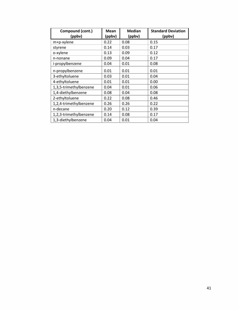
41
Compound (cont.) (ppbv)
Mean (ppbv)
Median (ppbv)
Standard Deviation (ppbv)
m+p-xylene 0.22 0.08 0.15 styrene 0.14 0.03 0.17 o-xylene 0.13 0.09 0.12 n-nonane 0.09 0.04 0.17 i-propylbenzene 0.04 0.01 0.08
n-propylbenzene 0.01 0.01 0.01 3-ethyltoluene 0.03 0.01 0.04 4-ethyltoluene 0.01 0.01 0.00 1,3,5-trimethylbenzene 0.04 0.01 0.06 1,4-diethylbenzene 0.08 0.04 0.08 2-ethyltoluene 0.22 0.08 0.46 1,2,4-trimethylbenzene 0.26 0.26 0.22 n-decane 0.20 0.12 0.39 1,2,3-trimethylbenzene 0.14 0.08 0.17 1,3-diethylbenzene 0.04 0.01 0.04

42
Appendix B Gas Chromatography System Calibration Statistics
Table B.1 contains calibration statistics for the ethane and VOCs measured on the multi-channel system. Table B.1. Calibration statistics for ethane and VOCs measured using the multi-channel GC system.
Compound Calibration r2 LOD (ppbv)
Slope of the Calibration Curve (peak area/ppbv)
Standard Range (ppbv)
ethane 0.999 0.105 137 0.4-3362
propane 0.999 0.020 1294 0.4-3203
i-butane 0.999 0.008 1682 0.4-3171
n-butane 0.999 0.010 1691 0.4-3140
cyclopentane 0.999 0.009 2097 0.4-3171
i-pentane 0.999 0.009 2110 0.4-3171
n-pentane 0.998 0.007 2039 0.4-3108
2,4-dimethylpentane 0.992 0.004 4049 0.4-3330
2,3-dimethylpentane 0.998 0.013 1049 0.4-3362
2,2,4-trimethylpentane 0.998 0.018 1196 0.4-3298
2,3,4-trimethylpentane 0.999 0.009 1174 0.4-3299
n-hexane 0.999 0.012 2467 0.4-3267
2-methylhexane 0.999 0.010 1079 0.4-3299
3-methylhexane 0.999 0.014 1064 0.4-3299
n-heptane 0.995 0.009 3164 0.4-3299
2-methylheptane 0.999 0.022 1165 0.4-3299
3-methylheptane 0.999 0.016 1177 0.4-3267
n-octane 0.999 0.016 1115 0.4-3299
n-nonane 0.999 0.010 1165 0.4-3235
n-decane 0.999 0.011 1131 0.4-3299
cyclohexane 0.999 0.015 895 0.4-3330
methylcyclohexane 0.999 0.019 1058 0.4-3299
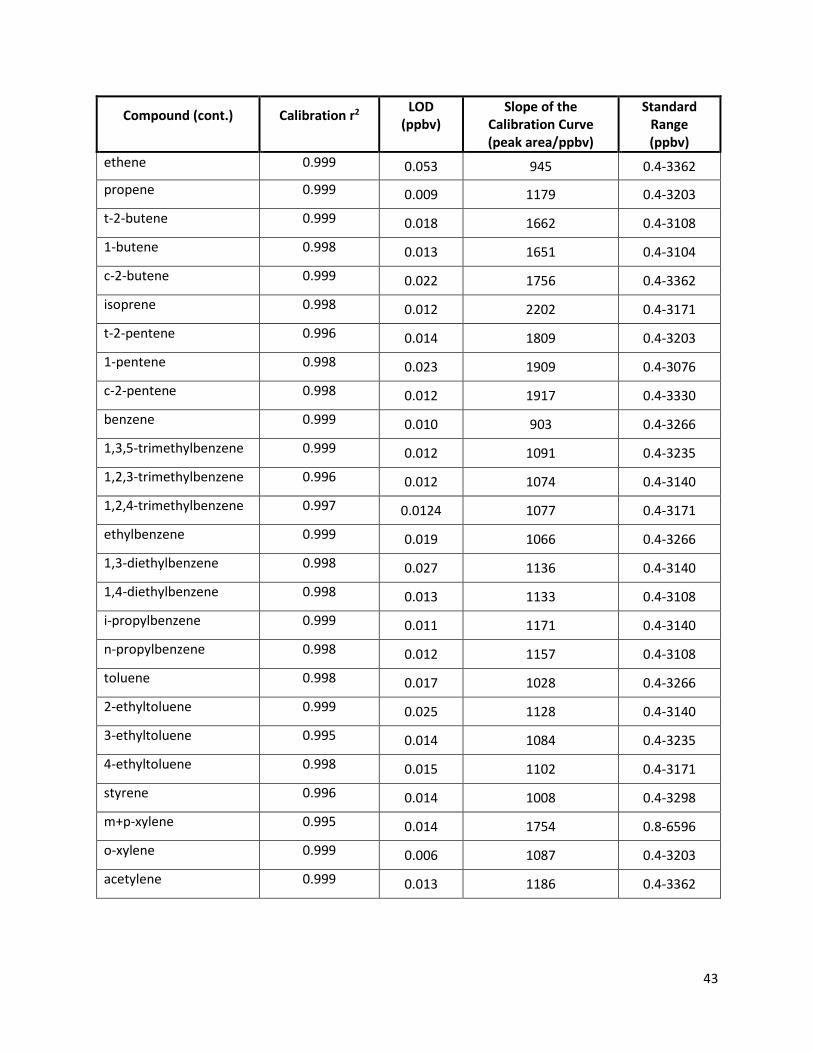
43
Compound (cont.) Calibration r2 LOD (ppbv)
Slope of the Calibration Curve (peak area/ppbv)
Standard Range (ppbv)
ethene 0.999 0.053 945 0.4-3362 propene 0.999 0.009 1179 0.4-3203
t-2-butene 0.999 0.018 1662 0.4-3108
1-butene 0.998 0.013 1651 0.4-3104
c-2-butene 0.999 0.022 1756 0.4-3362
isoprene 0.998 0.012 2202 0.4-3171
t-2-pentene 0.996 0.014 1809 0.4-3203
1-pentene 0.998 0.023 1909 0.4-3076
c-2-pentene 0.998 0.012 1917 0.4-3330
benzene 0.999 0.010 903 0.4-3266
1,3,5-trimethylbenzene 0.999 0.012 1091 0.4-3235
1,2,3-trimethylbenzene 0.996 0.012 1074 0.4-3140
1,2,4-trimethylbenzene 0.997 0.0124 1077 0.4-3171
ethylbenzene 0.999 0.019 1066 0.4-3266
1,3-diethylbenzene 0.998 0.027 1136 0.4-3140
1,4-diethylbenzene 0.998 0.013 1133 0.4-3108
i-propylbenzene 0.999 0.011 1171 0.4-3140
n-propylbenzene 0.998 0.012 1157 0.4-3108
toluene 0.998 0.017 1028 0.4-3266
2-ethyltoluene 0.999 0.025 1128 0.4-3140
3-ethyltoluene 0.995 0.014 1084 0.4-3235
4-ethyltoluene 0.998 0.015 1102 0.4-3171
styrene 0.996 0.014 1008 0.4-3298
m+p-xylene 0.995 0.014 1754 0.8-6596
o-xylene 0.999 0.006 1087 0.4-3203
acetylene 0.999 0.013 1186 0.4-3362

44
Appendix C Real-time Methane ERs for Individual Experiments
Figures C.1 to C.18 show the normalized frequency distribution of real-time methane ERs for experiments where the data satisfied the conditions set in Section 2.3.1. T is the number of hours of data available. Data were collected at 3Hz. The methane ERs for each experiment have been presented as a box and whisker plot. For all box and whisker figures in this Appendix, the blue line is the median, top and bottom of the box, and top and bottom whiskers are the 75th and 25th and the 95th and 5th percentiles respectively. The circles are all the data above or below 95th and 5st percentiles.
Figure C.1. Methane ER normalized frequency distributions from Experiment #1.
0.0
0.2
0.4
0.6
0.8
1.0
1.E-05 1.E-03 1.E-01 1.E+01 1.E+03
Nor
mal
ized
Freq
uenc
y
Methane Emission Rate (gs-1)
T=0.5hr45.6% Below DetectionProduction
CH4 E
R (g
s-1)
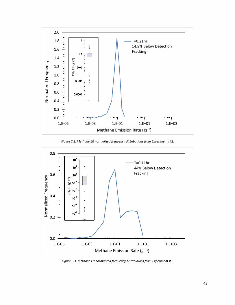
45
Figure C.2. Methane ER normalized frequency distributions from Experiments #2.
Figure C.3. Methane ER normalized frequency distributions from Experiment #3.
0.0
0.2
0.4
0.6
0.8
1.0
1.2
1.4
1.6
1.8
2.0
1.E-05 1.E-03 1.E-01 1.E+01 1.E+03
Nor
mal
ized
Freq
uenc
y
Methane Emission Rate (gs-1)
T=0.21hr14.8% Below DetectionFracking
0.0
0.2
0.4
0.6
0.8
1.E-05 1.E-03 1.E-01 1.E+01 1.E+03
Nor
mal
ized
Freq
uenc
y
Methane Emission Rate (gs-1)
T=0.11hr44% Below DetectionFracking
CH4 E
R (g
s-1)
CH4 E
R (g
s-1)
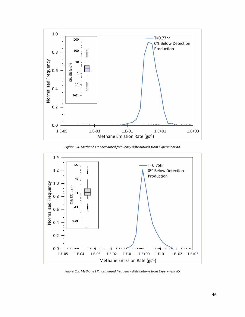
46
Figure C.4. Methane ER normalized frequency distributions from Experiment #4.
Figure C.5. Methane ER normalized frequency distributions from Experiment #5.
0.0
0.2
0.4
0.6
0.8
1.0
1.E-05 1.E-03 1.E-01 1.E+01 1.E+03
Nor
mal
ized
Freq
uenc
y
Methane Emission Rate (gs-1)
T=0.77hr0% Below DetectionProduction
0.0
0.2
0.4
0.6
0.8
1.0
1.2
1.4
1.E-05 1.E-04 1.E-03 1.E-02 1.E-01 1.E+00 1.E+01 1.E+02 1.E+03
Nor
mal
ized
Freq
uenc
y
Methane Emission Rate (gs-1)
T=0.75hr0% Below DetectionProduction
CH4 E
R (g
s-1)
CH4 E
R (g
s-1)
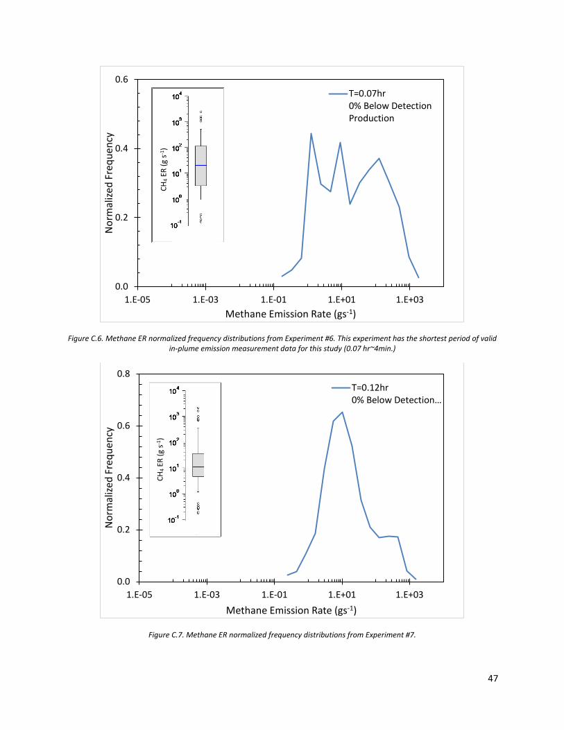
47
Figure C.6. Methane ER normalized frequency distributions from Experiment #6. This experiment has the shortest period of valid in-plume emission measurement data for this study (0.07 hr~4min.)
Figure C.7. Methane ER normalized frequency distributions from Experiment #7.
0.0
0.2
0.4
0.6
1.E-05 1.E-03 1.E-01 1.E+01 1.E+03
Nor
mal
ized
Freq
uenc
y
Methane Emission Rate (gs-1)
T=0.07hr0% Below DetectionProduction
0.0
0.2
0.4
0.6
0.8
1.E-05 1.E-03 1.E-01 1.E+01 1.E+03
Nor
mal
ized
Freq
uenc
y
Methane Emission Rate (gs-1)
T=0.12hr0% Below Detection…
CH4 E
R (g
s-1)
CH4 E
R (g
s-1)

48
Figure C.8. Methane ER normalized frequency distributions from Experiment #8.
Figure C.9. Methane ER normalized frequency distributions from Experiment #9.
0.0
0.2
0.4
0.6
0.8
1.E-05 1.E-04 1.E-03 1.E-02 1.E-01 1.E+00 1.E+01 1.E+02 1.E+03 1.E+04
Nor
mal
ized
Freq
uenc
y
Methane Emission Rate (gs-1)
T=0.07hr6.2% Below DetectionLiquids Load Out
0.0
0.2
0.4
0.6
1.E-05 1.E-03 1.E-01 1.E+01 1.E+03
Nor
mal
ized
Freq
uenc
y
Methane Emission Rate (gs-1)
T=0.32hr2.3% Below DetectionFlowback
CH4 E
R (g
s-1)
CH4 E
R (g
s-1)

49
Figure C.10. Methane ER normalized frequency distributions from Experiment #10.
Figure C.11. Methane ER normalized frequency distributions from Experiment #11.
0.0
0.2
0.4
0.6
0.8
1.0
1.E-05 1.E-03 1.E-01 1.E+01 1.E+03
Nor
mal
ized
Freq
uenc
y
Methane Emission Rate (gs-1)
T=0.29hr22.4% Below DetectionFlowback
0.0
0.2
0.4
0.6
1.E-05 1.E-03 1.E-01 1.E+01 1.E+03
Nor
mal
ized
Freq
uenc
y
Methane Emission Rate (gs-1)
T=0.25hr13.7% Below DetectionFracking
CH4 E
R (g
s-1)
CH4 E
R (g
s-1)
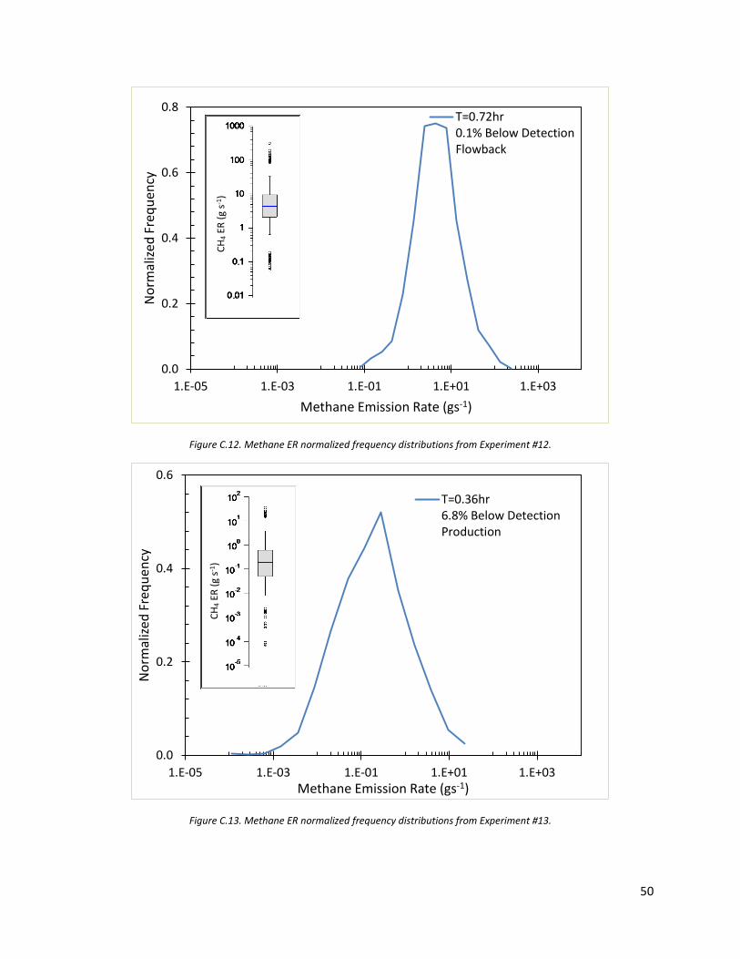
50
Figure C.12. Methane ER normalized frequency distributions from Experiment #12.
Figure C.13. Methane ER normalized frequency distributions from Experiment #13.
0.0
0.2
0.4
0.6
0.8
1.E-05 1.E-03 1.E-01 1.E+01 1.E+03
Nor
mal
ized
Freq
uenc
y
Methane Emission Rate (gs-1)
T=0.72hr0.1% Below DetectionFlowback
0.0
0.2
0.4
0.6
1.E-05 1.E-03 1.E-01 1.E+01 1.E+03
Nor
mal
ized
Freq
uenc
y
Methane Emission Rate (gs-1)
T=0.36hr6.8% Below DetectionProduction
CH4 E
R (g
s-1)
CH4 E
R (g
s-1)

51
Figure C.14. Methane ER normalized frequency distributions from Experiment #14.
Figure C.15. Methane ER normalized frequency distributions from Experiment #15.
0.0
0.2
0.4
0.6
1.E-05 1.E-03 1.E-01 1.E+01 1.E+03
Nor
mal
ized
Freq
uenc
y
Methane Emission Rate (gs-1)
T=0.78hr40.5% Below DetectionProduction
0.0
0.2
0.4
0.6
1.E-05 1.E-03 1.E-01 1.E+01 1.E+03
Nor
mal
ized
Freq
uenc
y
Methane Emission Rate (gs-1)
T=0.30hr20.7% Below DetectionProduction
CH4 E
R (g
s-1)
CH4 E
R (g
s-1)

52
Figure C.16. Methane ER normalized frequency distributions from Experiment #16.
Figure C.17. Methane ER normalized frequency distributions from Experiment #17.
0.0
0.2
0.4
0.6
1.E-05 1.E-03 1.E-01 1.E+01 1.E+03
Nor
mal
ized
Freq
uenc
y
Methane Emission Rate (gs-1)
T=0.15hr3.6% Below DetectionProduction
0.0
0.2
0.4
0.6
0.8
1.E-05 1.E-03 1.E-01 1.E+01 1.E+03
Nor
mal
ized
Freq
uenc
y
Methane Emission Rate (gs-1)
T=0.18hr1.4% Below DetectionProduction
CH4 E
R (g
s-1)
CH4 E
R (g
s-1)

53
Figure C.18. Methane ER normalized frequency distributions from Experiment #18.
0.0
0.2
0.4
0.6
0.8
1.E-05 1.E-04 1.E-03 1.E-02 1.E-01 1.E+00 1.E+01 1.E+02 1.E+03 1.E+04
Nor
mal
ized
Freq
uenc
y
Methane Emission Rate (gs-1)
T=0.15hr0% Below DetectionProduction
CH4 E
R (g
s-1)

54
Appendix D Canister Ethane and VOC ERs for Individual Experiments
The following figures present ERs of VOCs and ethane from individual experiments.
Figure D.1. ERs of VOCs and ethane from canisters collected during experiment #1. The bottom and top of the boxes are the 25th and 75th percentiles, the blue line inside the box represents the median, and the bottom and top whiskers are the 5th and 95th percentiles.
10-6
10-5
10-4
10-3
10-2
10-1
100
101
102
Emis
sion
Rat
es (g
s-1
)
etha
nepr
opan
ei-b
utan
en-
buta
nei-p
enta
nen-
pent
ane
2,3-
dim
ethy
lpen
tane
2,4-
dim
ethy
lpen
tane
2,2,
4-tri
met
hylp
enta
ne2,
3,4-
trim
ethy
lpen
tane
n-he
xane
2-m
ethy
lhex
ane
3-m
ethy
lhex
ane
n-he
ptan
e2-
met
hylh
epta
ne3-
met
hylh
epta
nen-
octa
nen-
nona
nen-
deca
neet
hene
prop
ene
t-2-b
uten
e1-
bute
nec-
2-bu
tene
t-2-p
ente
ne1-
pent
ene
c-2-
pent
ene
cycl
open
tane
cycl
ohex
ane
met
hylc
yclo
hexa
neis
opre
nebe
nzen
eto
luen
eet
hylb
enze
nem
+p-x
ylen
eso-
xyle
nest
yren
ei-p
ropy
lben
zene
n-pr
opyl
benz
ene
1,2,
3-tri
met
hylb
enze
ne1,
2,4-
trim
ethy
lben
zene
1,3,
5-tri
met
hylb
enze
ne1,
3-di
ethy
lben
zene
1,4-
diet
hylb
enze
ne2-
ethy
ltolu
ene
3-et
hylto
luen
e4-
ethy
ltolu
ene
Experiment #1Productionn = 10 canisters

55
Figure D.2. ERs of VOCs and ethane from canisters collected during experiment #2. The bottom and top of the boxes are the 25th and 75th percentiles, the blue line inside the box represents the median, and the bottom and top whiskers are the 5th and 95th percentiles.
Figure D.3. ERs of VOCs and ethane from canisters collected during experiment #3. The bottom and top of the boxes are the 25th and 75th percentiles, the blue line inside the box represents the median, and the bottom and top whiskers are the 5th and 95th percentiles.
10-6
10-5
10-4
10-3
10-2
10-1
100
101
102Em
issi
on R
ates
(g s
-1)
etha
nepr
opan
ei-b
utan
en-
buta
nei-p
enta
nen-
pent
ane
2,3-
dim
ethy
lpen
tane
2,4-
dim
ethy
lpen
tane
2,2,
4-tri
met
hylp
enta
ne2,
3,4-
trim
ethy
lpen
tane
n-he
xane
2-m
ethy
lhex
ane
3-m
ethy
lhex
ane
n-he
ptan
e2-
met
hylh
epta
ne3-
met
hylh
epta
nen-
octa
nen-
nona
nen-
deca
neet
hene
prop
ene
t-2-b
uten
e1-
bute
nec-
2-bu
tene
t-2-p
ente
ne1-
pent
ene
c-2-
pent
ene
cycl
open
tane
cycl
ohex
ane
met
hylc
yclo
hexa
neis
opre
nebe
nzen
eto
luen
eet
hylb
enze
nem
+p-x
ylen
eo-
xyle
nest
yren
ei-p
ropy
lben
zene
n-pr
opyl
benz
ene
1,2,
3-tri
met
hylb
enze
ne1,
2,4-
trim
ethy
lben
zene
1,3,
5-tri
met
hylb
enze
ne1,
3-di
ethy
lben
zene
1,4-
diet
hylb
enze
ne2-
ethy
ltolu
ene
3-et
hylto
luen
e4-
ethy
ltolu
ene
Experiment #2Frackingn = 10 canisters
10-6
10-5
10-4
10-3
10-2
10-1
100
101
102
Emis
sion
Rat
es (g
s-1
)
etha
nepr
opan
ei-b
utan
en-
buta
nei-p
enta
nen-
pent
ane
2,3-
dim
ethy
lpen
tane
2,4-
dim
ethy
lpen
tane
2,2,
4-tri
met
hylp
enta
ne2,
3,4-
trim
ethy
lpen
tane
n-he
xane
2-m
ethy
lhex
ane
3-m
ethy
lhex
ane
n-he
ptan
e2-
met
hylh
epta
ne3-
met
hylh
epta
nen-
octa
nen-
nona
nen-
deca
neet
hene
prop
ene
t-2-b
uten
e1-
bute
nec-
2-bu
tene
t-2-p
ente
ne1-
pent
ene
c-2-
pent
ene
cycl
open
tane
cycl
ohex
ane
met
hylc
yclo
hexa
neis
opre
nebe
nzen
eto
luen
eet
hylb
enze
nem
+p-x
ylen
eo-
xyle
nest
yren
ei-p
ropy
lben
zene
n-pr
opyl
benz
ene
1,2,
3-tri
met
hylb
enze
ne1,
2,4-
trim
ethy
lben
zene
1,3,
5-tri
met
hylb
enze
ne1,
3-di
ethy
lben
zene
1,4-
diet
hylb
enze
ne2-
ethy
ltolu
ene
3-et
hylto
luen
e4-
ethy
ltolu
ene
Experiment #3Frackingn = 14 canisters
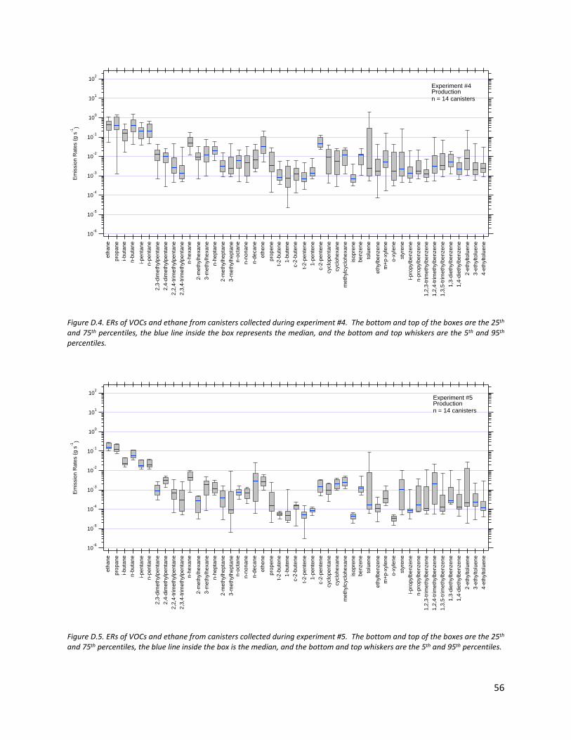
56
Figure D.4. ERs of VOCs and ethane from canisters collected during experiment #4. The bottom and top of the boxes are the 25th and 75th percentiles, the blue line inside the box represents the median, and the bottom and top whiskers are the 5th and 95th percentiles.
Figure D.5. ERs of VOCs and ethane from canisters collected during experiment #5. The bottom and top of the boxes are the 25th and 75th percentiles, the blue line inside the box is the median, and the bottom and top whiskers are the 5th and 95th percentiles.
10-6
10-5
10-4
10-3
10-2
10-1
100
101
102Em
issi
on R
ates
(g s
-1)
etha
nepr
opan
ei-b
utan
en-
buta
nei-p
enta
nen-
pent
ane
2,3-
dim
ethy
lpen
tane
2,4-
dim
ethy
lpen
tane
2,2,
4-tri
met
hylp
enta
ne2,
3,4-
trim
ethy
lpen
tane
n-he
xane
2-m
ethy
lhex
ane
3-m
ethy
lhex
ane
n-he
ptan
e2-
met
hylh
epta
ne3-
met
hylh
epta
nen-
octa
nen-
nona
nen-
deca
neet
hene
prop
ene
t-2-b
uten
e1-
bute
nec-
2-bu
tene
t-2-p
ente
ne1-
pent
ene
c-2-
pent
ene
cycl
open
tane
cycl
ohex
ane
met
hylc
yclo
hexa
neis
opre
nebe
nzen
eto
luen
eet
hylb
enze
nem
+p-x
ylen
eo-
xyle
nest
yren
ei-p
ropy
lben
zene
n-pr
opyl
benz
ene
1,2,
3-tri
met
hylb
enze
ne1,
2,4-
trim
ethy
lben
zene
1,3,
5-tri
met
hylb
enze
ne1,
3-di
ethy
lben
zene
1,4-
diet
hylb
enze
ne2-
ethy
ltolu
ene
3-et
hylto
luen
e4-
ethy
ltolu
ene
Experiment #4Productionn = 14 canisters
10-6
10-5
10-4
10-3
10-2
10-1
100
101
102
Emis
sion
Rat
es (g
s-1
)
etha
nepr
opan
ei-b
utan
en-
buta
nei-p
enta
nen-
pent
ane
2,3-
dim
ethy
lpen
tane
2,4-
dim
ethy
lpen
tane
2,2,
4-tri
met
hylp
enta
ne2,
3,4-
trim
ethy
lpen
tane
n-he
xane
2-m
ethy
lhex
ane
3-m
ethy
lhex
ane
n-he
ptan
e2-
met
hylh
epta
ne3-
met
hylh
epta
nen-
octa
nen-
nona
nen-
deca
neet
hene
prop
ene
t-2-b
uten
e1-
bute
nec-
2-bu
tene
t-2-p
ente
ne1-
pent
ene
c-2-
pent
ene
cycl
open
tane
cycl
ohex
ane
met
hylc
yclo
hexa
neis
opre
nebe
nzen
eto
luen
eet
hylb
enze
nem
+p-x
ylen
eo-
xyle
nest
yren
ei-p
ropy
lben
zene
n-pr
opyl
benz
ene
1,2,
3-tri
met
hylb
enze
ne1,
2,4-
trim
ethy
lben
zene
1,3,
5-tri
met
hylb
enze
ne1,
3-di
ethy
lben
zene
1,4-
diet
hylb
enze
ne2-
ethy
ltolu
ene
3-et
hylto
luen
e4-
ethy
ltolu
ene
Experiment #5Productionn = 14 canisters

57
Figure D.6. ERs of VOCs and ethane from canisters collected during experiment #6. The bottom and top of the boxes are the 25th and 75th percentiles, the blue line inside the box represents the median, and the bottom and top whiskers are the 5th and 95th percentiles.
Figure D.7. ERs of VOCs and ethane from canisters collected during experiment #7. The bottom and top of the boxes are the 25th and 75th percentiles, the blue line inside the box represents the median, the bottom and top whiskers are the 5th and 95th percentiles, and the asterisks are the outliers beyond the 5th and 95th percentiles.
10-6
10-5
10-4
10-3
10-2
10-1
100
101
102Em
issi
on R
ates
(g s
-1)
etha
nepr
opan
ei-b
utan
en-
buta
nei-p
enta
nen-
pent
ane
2,3-
dim
ethy
lpen
tane
2,4-
dim
ethy
lpen
tane
2,2,
4-tri
met
hylp
enta
ne2,
3,4-
trim
ethy
lpen
tane
n-he
xane
2-m
ethy
lhex
ane
3-m
ethy
lhex
ane
n-he
ptan
e2-
met
hylh
epta
ne3-
met
hylh
epta
nen-
octa
nen-
nona
nen-
deca
neet
hene
prop
ene
t-2-b
uten
e1-
bute
nec-
2-bu
tene
t-2-p
ente
ne1-
pent
ene
c-2-
pent
ene
cycl
open
tane
cycl
ohex
ane
met
hylc
yclo
hexa
neis
opre
nebe
nzen
eto
luen
eet
hylb
enze
nem
+p-x
ylen
eo-
xyle
nest
yren
ei-p
ropy
lben
zene
n-pr
opyl
benz
ene
1,2,
3-tri
met
hylb
enze
ne1,
2,4-
trim
ethy
lben
zene
1,3,
5-tri
met
hylb
enze
ne1,
3-di
ethy
lben
zene
1,4-
diet
hylb
enze
ne2-
ethy
ltolu
ene
3-et
hylto
luen
e4-
ethy
ltolu
ene
Experiment #6Productionn = 14 canisters
10-6
10-5
10-4
10-3
10-2
10-1
100
101
102
Emis
sion
Rat
es (g
s-1
)
etha
nepr
opan
ei-b
utan
en-
buta
nei-p
enta
nen-
pent
ane
2,3-
dim
ethy
lpen
tane
2,4-
dim
ethy
lpen
tane
2,2,
4-tri
met
hylp
enta
ne2,
3,4-
trim
ethy
lpen
tane
n-he
xane
2-m
ethy
lhex
ane
3-m
ethy
lhex
ane
n-he
ptan
e2-
met
hylh
epta
ne3-
met
hylh
epta
nen-
octa
nen-
nona
nen-
deca
neet
hene
prop
ene
t-2-b
uten
e1-
bute
nec-
2-bu
tene
t-2-p
ente
ne1-
pent
ene
c-2-
pent
ene
cycl
open
tane
cycl
ohex
ane
met
hylc
yclo
hexa
neis
opre
nebe
nzen
eto
luen
eet
hylb
enze
nem
+p-x
ylen
eo-
xyle
nest
yren
ei-p
ropy
lben
zene
n-pr
opyl
benz
ene
1,2,
3-tri
met
hylb
enze
ne1,
2,4-
trim
ethy
lben
zene
1,3,
5-tri
met
hylb
enze
ne1,
3-di
ethy
lben
zene
1,4-
diet
hylb
enze
ne2-
ethy
ltolu
ene
3-et
hylto
luen
e4-
ethy
ltolu
ene
Experiment #7Productionn = 15 canisters

58
Figure D.8. ERs of VOCs and ethane from canisters collected during experiment #8. The bottom and top of the boxes are the 25th and 75th percentiles, the blue line inside the box represents the median, and the bottom and top whiskers are the 5th and 95th percentiles.
Figure D.9. ERs of VOCs and ethane from canisters collected during experiment #9. The bottom and top of the boxes are the 25th and 75th percentiles, the blue line inside the box represents the median the bottom and top whiskers are the 5th and 95th percentiles.
10-6
10-5
10-4
10-3
10-2
10-1
100
101
102Em
issi
on R
ates
(g s
-1)
etha
nepr
opan
ei-b
utan
en-
buta
nei-p
enta
nen-
pent
ane
2,3-
dim
ethy
lpen
tane
2,4-
dim
ethy
lpen
tane
2,2,
4-tri
met
hylp
enta
ne2,
3,4-
trim
ethy
lpen
tane
n-he
xane
2-m
ethy
lhex
ane
3-m
ethy
lhex
ane
n-he
ptan
e2-
met
hylh
epta
ne3-
met
hylh
epta
nen-
octa
nen-
nona
nen-
deca
neet
hene
prop
ene
t-2-b
uten
e1-
bute
nec-
2-bu
tene
t-2-p
ente
ne1-
pent
ene
c-2-
pent
ene
cycl
open
tane
cycl
ohex
ane
met
hylc
yclo
hexa
neis
opre
nebe
nzen
eto
luen
eet
hylb
enze
nem
+p-x
ylen
eo-
xyle
nest
yren
ei-p
ropy
lben
zene
n-pr
opyl
benz
ene
1,2,
3-tri
met
hylb
enze
ne1,
2,4-
trim
ethy
lben
zene
1,3,
5-tri
met
hylb
enze
ne1,
3-di
ethy
lben
zene
1,4-
diet
hylb
enze
ne2-
ethy
ltolu
ene
3-et
hylto
luen
e4-
ethy
ltolu
ene
Experiment #8Liquids Load Outn = 5 canisters
10-6
10-5
10-4
10-3
10-2
10-1
100
101
102
Emis
sion
Rat
es (g
s-1
)
etha
nepr
opan
ei-b
utan
en-
buta
nei-p
enta
nen-
pent
ane
2,3-
dim
ethy
lpen
tane
2,4-
dim
ethy
lpen
tane
2,2,
4-tri
met
hylp
enta
ne2,
3,4-
trim
ethy
lpen
tane
n-he
xane
2-m
ethy
lhex
ane
3-m
ethy
lhex
ane
n-he
ptan
e2-
met
hylh
epta
ne3-
met
hylh
epta
nen-
octa
nen-
nona
nen-
deca
neet
hene
prop
ene
t-2-b
uten
e1-
bute
nec-
2-bu
tene
t-2-p
ente
ne1-
pent
ene
c-2-
pent
ene
cycl
open
tane
cycl
ohex
ane
met
hylc
yclo
hexa
neis
opre
nebe
nzen
eto
luen
eet
hylb
enze
nem
+p-x
ylen
eo-
xyle
nest
yren
ei-p
ropy
lben
zene
n-pr
opyl
benz
ene
1,2,
3-tri
met
hylb
enze
ne1,
2,4-
trim
ethy
lben
zene
1,3,
5-tri
met
hylb
enze
ne1,
3-di
ethy
lben
zene
1,4-
diet
hylb
enze
ne2-
ethy
ltolu
ene
3-et
hylto
luen
e4-
ethy
ltolu
ene
Experiment #9Flowbackn = 13 canisters

59
Figure D.10. ERs of VOCs and ethane from canisters collected during experiment #10. The bottom and top of the boxes are the 25th and 75th percentiles, the blue line inside the box represents the median, and the bottom and top whiskers are the 5th and 95th percentiles.
Figure D.11. ERs of VOCs and ethane from canisters collected during experiment #11. The bottom and top of the boxes are the 25th and 75th percentiles, the blue line inside the box represents the median, and the bottom and top whiskers are the 5th and 95th percentiles.
10-6
10-5
10-4
10-3
10-2
10-1
100
101
102Em
issi
on R
ates
(g s
-1)
etha
nepr
opan
ei-b
utan
en-
buta
nei-p
enta
nen-
pent
ane
2,3-
dim
ethy
lpen
tane
2,4-
dim
ethy
lpen
tane
2,2,
4-tri
met
hylp
enta
ne2,
3,4-
trim
ethy
lpen
tane
n-he
xane
2-m
ethy
lhex
ane
3-m
ethy
lhex
ane
n-he
ptan
e2-
met
hylh
epta
ne3-
met
hylh
epta
nen-
octa
nen-
nona
nen-
deca
neet
hene
prop
ene
t-2-b
uten
e1-
bute
nec-
2-bu
tene
t-2-p
ente
ne1-
pent
ene
c-2-
pent
ene
cycl
open
tane
cycl
ohex
ane
met
hylc
yclo
hexa
neis
opre
nebe
nzen
eto
luen
eet
hylb
enze
nem
+p-x
ylen
eo-
xyle
nest
yren
ei-p
ropy
lben
zene
n-pr
opyl
benz
ene
1,2,
3-tri
met
hylb
enze
ne1,
2,4-
trim
ethy
lben
zene
1,3,
5-tri
met
hylb
enze
ne1,
3-di
ethy
lben
zene
1,4-
diet
hylb
enze
ne2-
ethy
ltolu
ene
3-et
hylto
luen
e4-
ethy
ltolu
ene
Experiment #10Flowbackn = 11 canisters
10-6
10-5
10-4
10-3
10-2
10-1
100
101
102
Emis
sion
Rat
es (g
s-1
)
etha
nepr
opan
ei-b
utan
en-
buta
nei-p
enta
nen-
pent
ane
2,3-
dim
ethy
lpen
tane
2,4-
dim
ethy
lpen
tane
2,2,
4-tri
met
hylp
enta
ne2,
3,4-
trim
ethy
lpen
tane
n-he
xane
2-m
ethy
lhex
ane
3-m
ethy
lhex
ane
n-he
ptan
e2-
met
hylh
epta
ne3-
met
hylh
epta
nen-
octa
nen-
nona
nen-
deca
neet
hene
prop
ene
t-2-b
uten
e1-
bute
nec-
2-bu
tene
t-2-p
ente
ne1-
pent
ene
c-2-
pent
ene
cycl
open
tane
cycl
ohex
ane
met
hylc
yclo
hexa
neis
opre
nebe
nzen
eto
luen
eet
hylb
enze
nem
+p-x
ylen
eo-
xyle
nest
yren
ei-p
ropy
lben
zene
n-pr
opyl
benz
ene
1,2,
3-tri
met
hylb
enze
ne1,
2,4-
trim
ethy
lben
zene
1,3,
5-tri
met
hylb
enze
ne1,
3-di
ethy
lben
zene
1,4-
diet
hylb
enze
ne2-
ethy
ltolu
ene
3-et
hylto
luen
e4-
ethy
ltolu
ene
Experiment #11Frackingn = 16 canisters

60
Figure D.12. ERs of VOCs and ethane from canisters collected during experiment #12. The bottom and top of the boxes are the 25th and 75th percentiles, the blue line inside the box represents the median, and the bottom and top whiskers are the 5th and 95th percentiles.
Figure D.13. ERs of VOCs and ethane from canisters collected during experiment #13. The bottom and top of the boxes are the 25th and 75th percentiles, the blue line inside the box represents the median, and the bottom and top whiskers are the 5th and 95th percentiles.
10-6
10-5
10-4
10-3
10-2
10-1
100
101
102Em
issi
on R
ates
(g s
-1)
etha
nepr
opan
ei-b
utan
en-
buta
nei-p
enta
nen-
pent
ane
2,3-
dim
ethy
lpen
tane
2,4-
dim
ethy
lpen
tane
2,2,
4-tri
met
hylp
enta
ne2,
3,4-
trim
ethy
lpen
tane
n-he
xane
2-m
ethy
lhex
ane
3-m
ethy
lhex
ane
n-he
ptan
e2-
met
hylh
epta
ne3-
met
hylh
epta
nen-
octa
nen-
nona
nen-
deca
neet
hene
prop
ene
t-2-b
uten
e1-
bute
nec-
2-bu
tene
t-2-p
ente
ne1-
pent
ene
c-2-
pent
ene
cycl
open
tane
cycl
ohex
ane
met
hylc
yclo
hexa
neis
opre
nebe
nzen
eto
luen
eet
hylb
enze
nem
+p-x
ylen
eo-
xyle
nest
yren
ei-p
ropy
lben
zene
n-pr
opyl
benz
ene
1,2,
3-tri
met
hylb
enze
ne1,
2,4-
trim
ethy
lben
zene
1,3,
5-tri
met
hylb
enze
ne1,
3-di
ethy
lben
zene
1,4-
diet
hylb
enze
ne2-
ethy
ltolu
ene
3-et
hylto
luen
e4-
ethy
ltolu
ene
Experiment #12Flowbackn = 12 canisters
10-6
10-5
10-4
10-3
10-2
10-1
100
101
102
Emis
sion
Rat
es (g
s-1
)
etha
nepr
opan
ei-b
utan
en-
buta
nei-p
enta
nen-
pent
ane
2,3-
dim
ethy
lpen
tane
2,4-
dim
ethy
lpen
tane
2,2,
4-tri
met
hylp
enta
ne2,
3,4-
trim
ethy
lpen
tane
n-he
xane
2-m
ethy
lhex
ane
3-m
ethy
lhex
ane
n-he
ptan
e2-
met
hylh
epta
ne3-
met
hylh
epta
nen-
octa
nen-
nona
nen-
deca
neet
hene
prop
ene
t-2-b
uten
e1-
bute
nec-
2-bu
tene
t-2-p
ente
ne1-
pent
ene
c-2-
pent
ene
cycl
open
tane
cycl
ohex
ane
met
hylc
yclo
hexa
neis
opre
nebe
nzen
eto
luen
eet
hylb
enze
nem
+p-x
ylen
eo-
xyle
nest
yren
ei-p
ropy
lben
zene
n-pr
opyl
benz
ene
1,2,
3-tri
met
hylb
enze
ne1,
2,4-
trim
ethy
lben
zene
1,3,
5-tri
met
hylb
enze
ne1,
3-di
ethy
lben
zene
1,4-
diet
hylb
enze
ne2-
ethy
ltolu
ene
3-et
hylto
luen
e4-
ethy
ltolu
ene
Experiment #13Productionn = 14 canisters
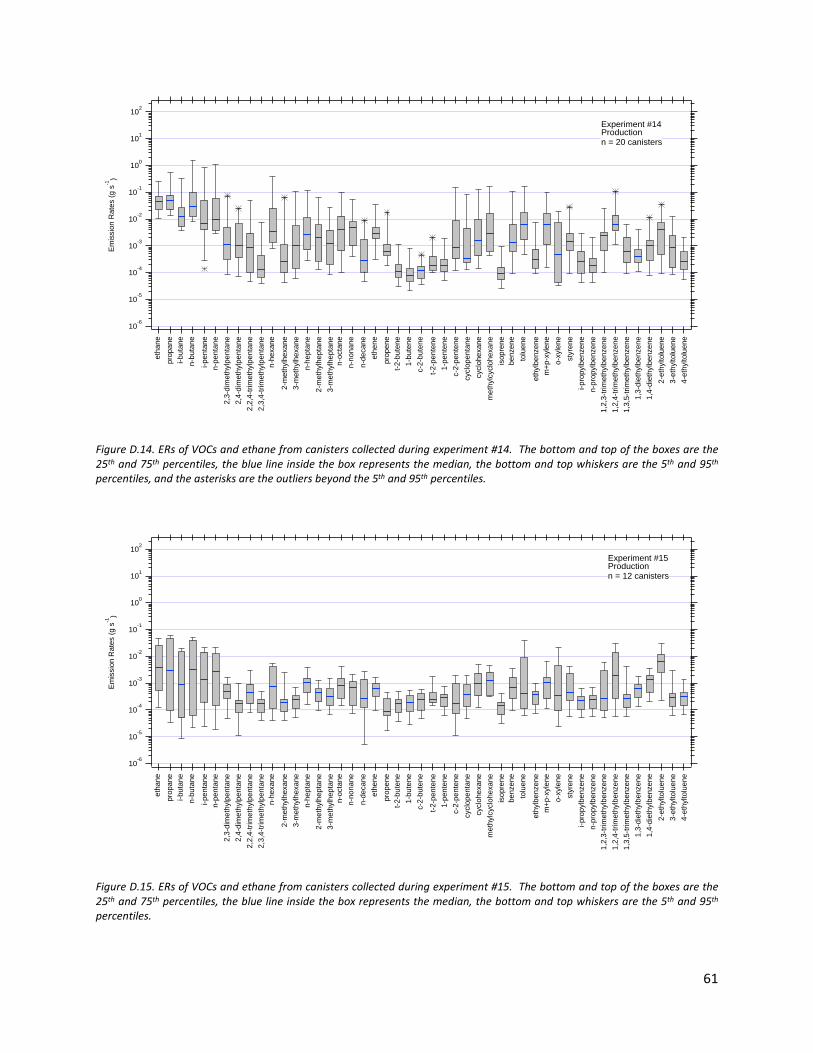
61
Figure D.14. ERs of VOCs and ethane from canisters collected during experiment #14. The bottom and top of the boxes are the 25th and 75th percentiles, the blue line inside the box represents the median, the bottom and top whiskers are the 5th and 95th percentiles, and the asterisks are the outliers beyond the 5th and 95th percentiles.
Figure D.15. ERs of VOCs and ethane from canisters collected during experiment #15. The bottom and top of the boxes are the 25th and 75th percentiles, the blue line inside the box represents the median, the bottom and top whiskers are the 5th and 95th percentiles.
10-6
10-5
10-4
10-3
10-2
10-1
100
101
102Em
issi
on R
ates
(g s
-1)
etha
nepr
opan
ei-b
utan
en-
buta
nei-p
enta
nen-
pent
ane
2,3-
dim
ethy
lpen
tane
2,4-
dim
ethy
lpen
tane
2,2,
4-tri
met
hylp
enta
ne2,
3,4-
trim
ethy
lpen
tane
n-he
xane
2-m
ethy
lhex
ane
3-m
ethy
lhex
ane
n-he
ptan
e2-
met
hylh
epta
ne3-
met
hylh
epta
nen-
octa
nen-
nona
nen-
deca
neet
hene
prop
ene
t-2-b
uten
e1-
bute
nec-
2-bu
tene
t-2-p
ente
ne1-
pent
ene
c-2-
pent
ene
cycl
open
tane
cycl
ohex
ane
met
hylc
yclo
hexa
neis
opre
nebe
nzen
eto
luen
eet
hylb
enze
nem
+p-x
ylen
eo-
xyle
nest
yren
ei-p
ropy
lben
zene
n-pr
opyl
benz
ene
1,2,
3-tri
met
hylb
enze
ne1,
2,4-
trim
ethy
lben
zene
1,3,
5-tri
met
hylb
enze
ne1,
3-di
ethy
lben
zene
1,4-
diet
hylb
enze
ne2-
ethy
ltolu
ene
3-et
hylto
luen
e4-
ethy
ltolu
ene
Experiment #14Productionn = 20 canisters
10-6
10-5
10-4
10-3
10-2
10-1
100
101
102
Emis
sion
Rat
es (g
s-1
)
etha
nepr
opan
ei-b
utan
en-
buta
nei-p
enta
nen-
pent
ane
2,3-
dim
ethy
lpen
tane
2,4-
dim
ethy
lpen
tane
2,2,
4-tri
met
hylp
enta
ne2,
3,4-
trim
ethy
lpen
tane
n-he
xane
2-m
ethy
lhex
ane
3-m
ethy
lhex
ane
n-he
ptan
e2-
met
hylh
epta
ne3-
met
hylh
epta
nen-
octa
nen-
nona
nen-
deca
neet
hene
prop
ene
t-2-b
uten
e1-
bute
nec-
2-bu
tene
t-2-p
ente
ne1-
pent
ene
c-2-
pent
ene
cycl
open
tane
cycl
ohex
ane
met
hylc
yclo
hexa
neis
opre
nebe
nzen
eto
luen
eet
hylb
enze
nem
+p-x
ylen
eo-
xyle
nest
yren
ei-p
ropy
lben
zene
n-pr
opyl
benz
ene
1,2,
3-tri
met
hylb
enze
ne1,
2,4-
trim
ethy
lben
zene
1,3,
5-tri
met
hylb
enze
ne1,
3-di
ethy
lben
zene
1,4-
diet
hylb
enze
ne2-
ethy
ltolu
ene
3-et
hylto
luen
e4-
ethy
ltolu
ene
Experiment #15Productionn = 12 canisters
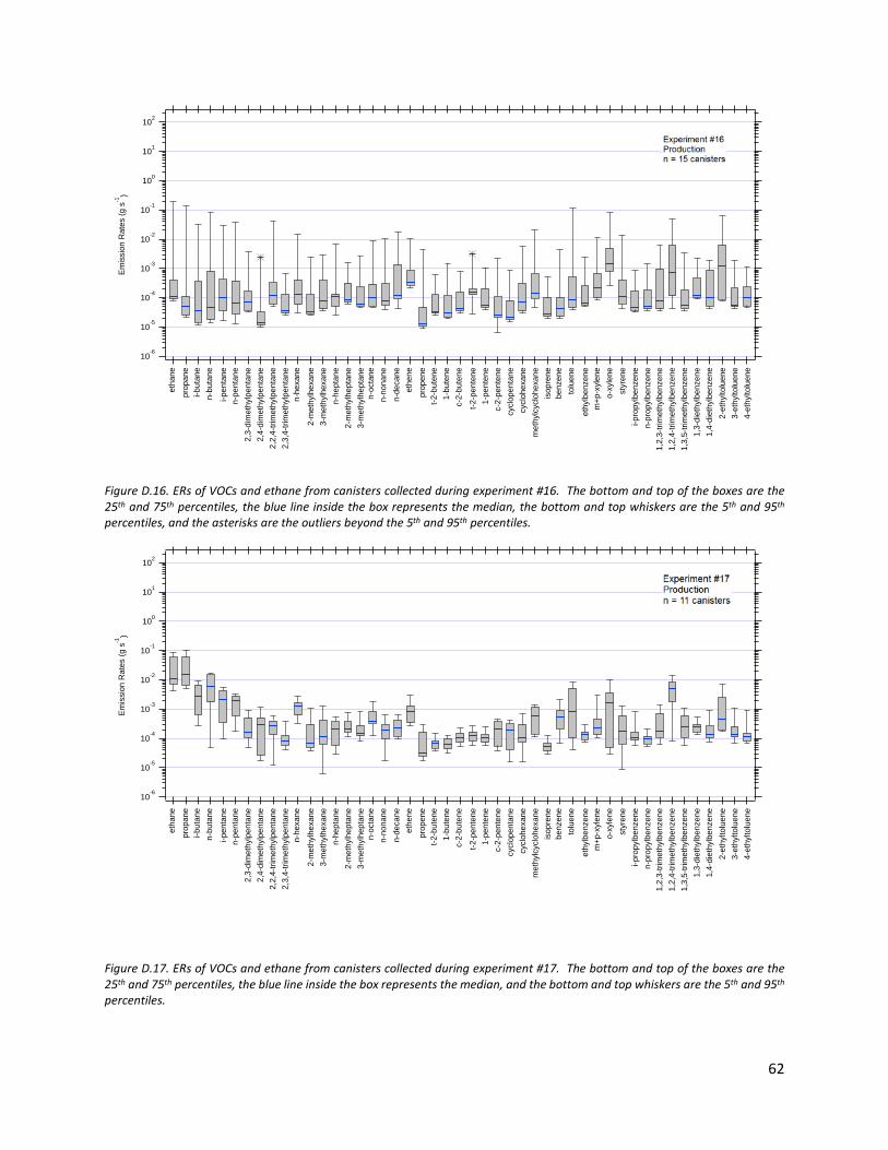
62
Figure D.16. ERs of VOCs and ethane from canisters collected during experiment #16. The bottom and top of the boxes are the 25th and 75th percentiles, the blue line inside the box represents the median, the bottom and top whiskers are the 5th and 95th percentiles, and the asterisks are the outliers beyond the 5th and 95th percentiles.
Figure D.17. ERs of VOCs and ethane from canisters collected during experiment #17. The bottom and top of the boxes are the 25th and 75th percentiles, the blue line inside the box represents the median, and the bottom and top whiskers are the 5th and 95th percentiles.
10-6
10-5
10-4
10-3
10-2
10-1
100
101
102Em
issi
on R
ates
(g s
-1)
etha
nepr
opan
ei-b
utan
en-
buta
nei-p
enta
nen-
pent
ane
2,3-
dim
ethy
lpen
tane
2,4-
dim
ethy
lpen
tane
2,2,
4-tri
met
hylp
enta
ne2,
3,4-
trim
ethy
lpen
tane
n-he
xane
2-m
ethy
lhex
ane
3-m
ethy
lhex
ane
n-he
ptan
e2-
met
hylh
epta
ne3-
met
hylh
epta
nen-
octa
nen-
nona
nen-
deca
neet
hene
prop
ene
t-2-b
uten
e1-
bute
nec-
2-bu
tene
t-2-p
ente
ne1-
pent
ene
c-2-
pent
ene
cycl
open
tane
cycl
ohex
ane
met
hylc
yclo
hexa
neis
opre
nebe
nzen
eto
luen
eet
hylb
enze
nem
+p-x
ylen
eo-
xyle
nest
yren
ei-p
ropy
lben
zene
n-pr
opyl
benz
ene
1,2,
3-tri
met
hylb
enze
ne1,
2,4-
trim
ethy
lben
zene
1,3,
5-tri
met
hylb
enze
ne1,
3-di
ethy
lben
zene
1,4-
diet
hylb
enze
ne2-
ethy
ltolu
ene
3-et
hylto
luen
e4-
ethy
ltolu
ene
Experiment #16Productionn = 10 canisters
10-6
10-5
10-4
10-3
10-2
10-1
100
101
102
Emis
sion
Rat
es (g
s-1
)
etha
nepr
opan
ei-b
utan
en-
buta
nei-p
enta
nen-
pent
ane
2,3-
dim
ethy
lpen
tane
2,4-
dim
ethy
lpen
tane
2,2,
4-tri
met
hylp
enta
ne2,
3,4-
trim
ethy
lpen
tane
n-he
xane
2-m
ethy
lhex
ane
3-m
ethy
lhex
ane
n-he
ptan
e2-
met
hylh
epta
ne3-
met
hylh
epta
nen-
octa
nen-
nona
nen-
deca
neet
hene
prop
ene
t-2-b
uten
e1-
bute
nec-
2-bu
tene
t-2-p
ente
ne1-
pent
ene
c-2-
pent
ene
cycl
open
tane
cycl
ohex
ane
met
hylc
yclo
hexa
neis
opre
nebe
nzen
eto
luen
eet
hylb
enze
nem
+p-x
ylen
eo-
xyle
nest
yren
ei-p
ropy
lben
zene
n-pr
opyl
benz
ene
1,2,
3-tri
met
hylb
enze
ne1,
2,4-
trim
ethy
lben
zene
1,3,
5-tri
met
hylb
enze
ne1,
3-di
ethy
lben
zene
1,4-
diet
hylb
enze
ne2-
ethy
ltolu
ene
3-et
hylto
luen
e4-
ethy
ltolu
ene
Experiment #17Productionn = 10 canisters

63
Figure D.18. ERs of VOCs and ethane from canisters collected during experiment #18. The bottom and top of the boxes are the 25th and 75th percentiles, the blue line inside the box represents the median, and the bottom and top whiskers are the 5th and 95th percentiles.
10-6
10-5
10-4
10-3
10-2
10-1
100
101
102Em
issi
on R
ates
(g s
-1)
etha
nepr
opan
ei-b
utan
en-
buta
nei-p
enta
nen-
pent
ane
2,3-
dim
ethy
lpen
tane
2,4-
dim
ethy
lpen
tane
2,2,
4-tri
met
hylp
enta
ne2,
3,4-
trim
ethy
lpen
tane
n-he
xane
2-m
ethy
lhex
ane
3-m
ethy
lhex
ane
n-he
ptan
e2-
met
hylh
epta
ne3-
met
hylh
epta
nen-
octa
nen-
nona
nen-
deca
neet
hene
prop
ene
t-2-b
uten
e1-
bute
nec-
2-bu
tene
t-2-p
ente
ne1-
pent
ene
c-2-
pent
ene
cycl
open
tane
cycl
ohex
ane
met
hylc
yclo
hexa
neis
opre
nebe
nzen
eto
luen
eet
hylb
enze
nem
+p-x
ylen
eo-
xyle
nest
yren
ei-p
ropy
lben
zene
n-pr
opyl
benz
ene
1,2,
3-tri
met
hylb
enze
ne1,
2,4-
trim
ethy
lben
zene
1,3,
5-tri
met
hylb
enze
ne1,
3-di
ethy
lben
zene
1,4-
diet
hylb
enze
ne2-
ethy
ltolu
ene
3-et
hylto
luen
e4-
ethy
ltolu
ene
Experiment #18Productionn = 11 canisters

64
Appendix E Site Descriptions for Individual Experiments
The following Tables present the description of the facilities present at the time of measurement.
Table E.1. Description of facilities for all the production sites.
Experiment #
Monthly gas (Msfc)
Monthly Condensate
(bbl) # of
Wells
# of Condensate
tank Stages of
Separation Well Type 1 613 18 9 3 1 Vertical 4 3128 1047 4 5 3 Horizontal 5 7197 707 11 0 Bulk Both 6 12378 1661 18 0 Bulk Horizontal 7 7715 1560 8 27 2 Horizontal
13 251 25 6 3 2 Both 14 1342 112 5 15 2 Horizontal 15 21 1.1 2 2 2 Vertical 16 5403 269 1 3 2 Horizontal 17 189 189 2 4 2 Vertical 18 4527 3477 4 8 2 Horizontal

65
Table E.2. Site description parameters for all fracking, flowback, and liquids load out experiments.
Experiment #
Type of Operation Notes # of
Wells Water
Management Stages of
Separation Duration Permanent Line Status
2 Fracking NA NA NA NA NA NA
3 Fracking NA NA NA NA NA NA
8 Liquids load out
NA NA NA NA NA NA
9 Flowback (Green)
1 well drill out 2 separators 6 Stored on site 3
3 weeks (1.5 weeks drill out)
Condensate and gas piped
from separators to permanent production facility and then sales pipeline
10 Flowback (Green)
1 well drill out 2 separators 6 Stored on site 3
3 weeks (1.5 weeks drill out)
Condensate and gas piped
from separators to permanent production facility and then sales pipeline
11 Fracking Approximately 350 stages 7
Source: 95% fresh
5% recycled NA 25 days
All wells shut in
(no condensate
or gas production)
12 Flowback (Green)
1 well drill out 2 separators 6 Stored on site 3
5 weeks (3 weeks of
drill out)
Condensate and gas piped
from separators to permanent production facility and then sales pipeline
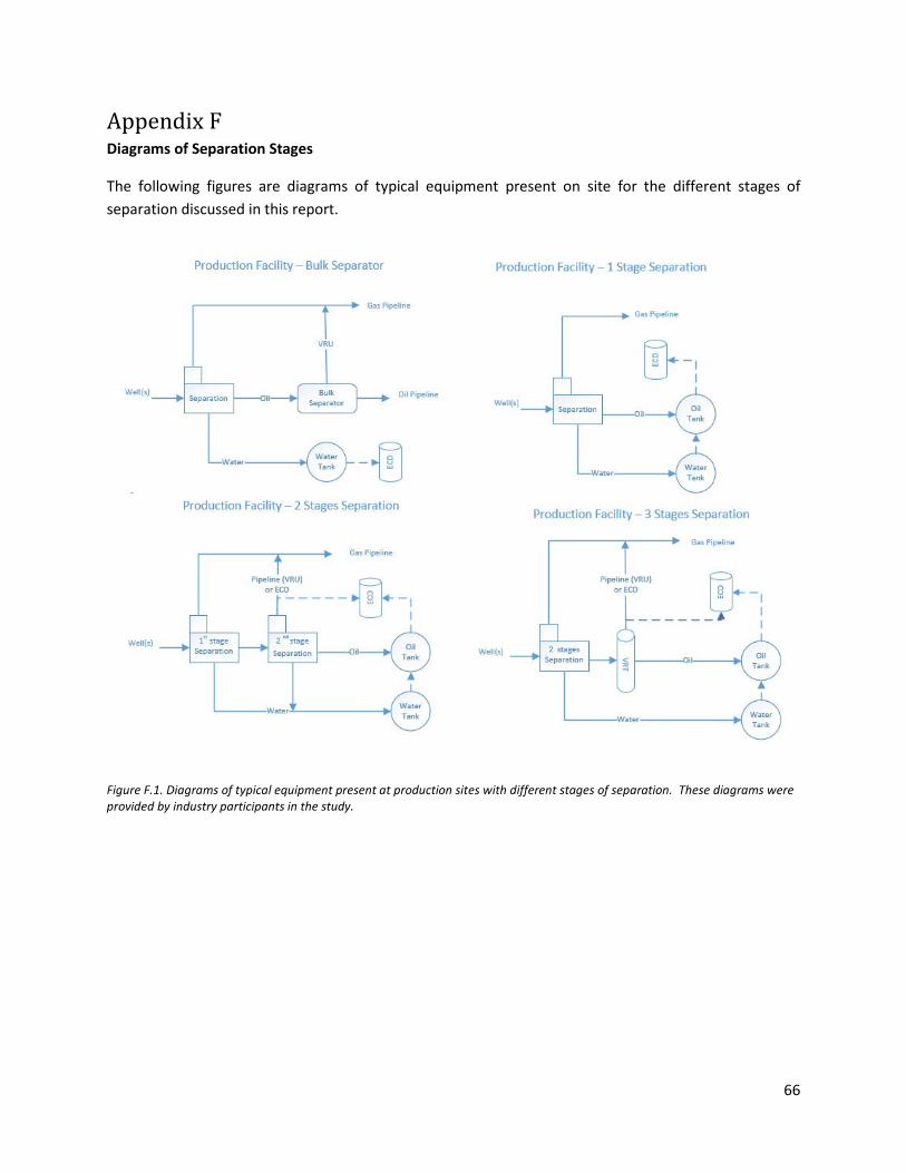
66
Appendix F Diagrams of Separation Stages
The following figures are diagrams of typical equipment present on site for the different stages of separation discussed in this report.
Figure F.1. Diagrams of typical equipment present at production sites with different stages of separation. These diagrams were provided by industry participants in the study.