NONLINEAR TRAVELING WAVES FOR THE SKELETON …stechmann/publications/ChenStechmann2016... ·...

NONLINEAR TRAVELING WAVES FOR THE SKELETON OF THEMADDEN–JULIAN OSCILLATION ∗

SHENGQIAN CHEN † AND SAMUEL N. STECHMANN ‡

Abstract. The Madden–Julian Oscillation (MJO) is the dominant component of intraseasonal(30–90 days) variability in the tropical atmosphere. Here, traveling wave solutions are presentedfor the MJO skeleton model of Majda and Stechmann. The model is a system of nonlinear partialdifferential equations that describe the evolution of the tropical atmosphere on planetary (10,000–40,000 km) spatial scales. The nonlinear traveling waves come in four types, corresponding to thefour types of linear wave solutions, one of which has the properties of the MJO. In the MJO travelingwave, the convective activity has a pulse-like shape, with a narrow region of enhanced convection anda wide region of suppressed convection. Furthermore, an amplitude-dependent dispersion relation isderived, and it shows that the nonlinear MJO has a lower frequency and slower propagation speedthan the linear MJO. By taking the small-amplitude limit, an analytic formula is also derived forthe dispersion relation of linear waves. To derive all of these results, a key aspect is the model’sconservation of energy, which holds even in the presence of forcing. In the limit of weak forcing, itis shown that the nonlinear traveling waves have a simple sech-squared waveform.

Key words. nonlinear traveling waves, solitary waves, tropical climate, tropical intraseasonalvariability, partial differential equations.

subject classifications. 74J30, 76B60, 35Q35, 76U05, 86A10

1. IntroductionThis paper concerns the following system of nonlinear partial differential equations

(PDEs):

Kt +Kx =−1

2(HA−F ) (1.1a)

Rt−1

3Rx =−1

3(HA−F ) (1.1b)

Qt +QKx−Q

3Rx = (

Q

6−1)(HA−F ) (1.1c)

At = ΓQA (1.1d)

which was originally designed in [33]. This is a hyperbolic system whose only nonlin-earity is in equation (1.1d). The main goals of this paper are (i) to present nonlineartraveling wave solutions of (1.1) and (ii) to describe the features of the nonlinear wavesthat are absent from the linear waves. An important element will be conservation ofenergy, which holds even in the presence of the source term, F .

In equations (1.1), the variables K, R, Q, and A represent the state of the at-mosphere near the equator. K and R represent Kelvin and equatorial Rossby wavecirculation patterns, and they are related to the velocity and temperature as de-scribed further below. Q represents the lower-tropospheric water vapor (“moisture”hereafter), and A represents the amplitude of deep convective activity. As such, Aaccounts for an important moisture sink and heat source for the atmosphere, fromrainfall and latent heating, as represented by the proportionality constant H for heat-ing.

∗Received: May 22, 2014. Revised: June 11, 2015. Accepted: June 15, 2015.†Department of Mathematics, University of Wisconsin at Madison, USA ([email protected]).

http://math.wisc.edu/∼sqchen‡Department of Mathematics, and Department of Atmospheric and Oceanic Sciences, University

of Wisconsin at Madison, USA ([email protected]). http://math.wisc.edu/∼stechmann

1

2 NONLINEAR TRAVELING WAVE SOLUTIONS FOR MJO SKELETON MODEL

The system (1.1) was proposed in [33] as a model for the Madden–Julian Oscil-lation (MJO). The MJO is the dominant component of intraseasonal (≈ 30-60 days)variability in the tropical atmosphere. This variability appears not only in the wind,pressure, and temperature fields, but also in water vapor and precipitation/convection.The structure of the MJO is a planetary-scale (≈ 10,000-40,000 km) circulation cellwith regions of enhanced and suppressed convection, and it propagates slowly east-ward at a speed of roughly 5 m/s. The main regions of MJO convective activity areover the Indian and western Pacific Oceans, and the MJO interacts with monsoons,tropical cyclones, El Nino–Southern Oscillation, and other tropical phenomena. Nev-ertheless, while the MJO is mainly a tropical phenomenon, it also interacts with theextratropics and can affect midlatitude predictability. See [21, 24–26, 47] for furtherbackground information on the MJO.

Despite the wealth of studies dedicated to the MJO, theory and numerical simula-tions are still major challenges. Several studies have documented the inadequacies andprogress of general circulation model (GCM) simulations [18, 23, 41], and new tech-niques continue to be developed and show increasingly realistic results [1,2,12,17]. Alarge part of the challenge is the complex multiscale structure of the MJO [7, 14, 38].More theoretical work is needed to better understand the multiscale processes at workin the tropics. For recent reviews, see [16,19,36].

Motivated by the MJO’s multiscale structure, the terminology of the MJO’s“skeleton” and “muscle” was introduced in [33], and it refers to the MJO’sintraseasonal–planetary-scale envelope and further details beyond the envelope, re-spectively. Further work with the MJO skeleton model can be found in [33, 34, 44],including a stochastic version of the model [44]. Work on the MJO’s “muscle” canbe found in [5, 15, 29, 32, 43], which focus on the role of convective momentum trans-port [37].

In addition to (1.1), which includes effects of the Coriolis force and meridional (y)variations of the circulation, a simpler yet less realistic system will also be consideredhere:

ut−θx = 0 (1.2a)

θt−ux = Ha−F (1.2b)

qt +Qux =−Ha+F (1.2c)

at = Γqa (1.2d)

where u is a velocity and θ represents a temperature [33]. This system neglectsmeridional (y) variations and can be thought of as the atmospheric circulation directlyabove the equator, y= 0, where the Coriolis force vanishes. Many of the results herewill hold equally well for (1.1) and (1.2). While (1.2) neglects important physics, theireast–west symmetry is mathematically advantageous, as it provides a simplificationof the equations. Also, these equations have the advantage of being written in termsof zonal velocity u and potential temperature θ, which are more physically intuitivethan the wave amplitude variables K and R.

The nonlinear traveling waves of the present paper are an addition to severalsolitary wave systems for other atmospheric phenomena. Several examples take theform of coupled KdV systems, including some with nonlinear self-interaction and lin-ear coupling [11, 35] and some with nonlinear coupling [3, 4, 13, 28, 39]. The linearlycoupled systems [11, 35] were derived in the context of midlatitude baroclinic insta-bility, and the nonlinearly coupled system [28] was derived in the context of tropical–

S. CHEN and S. N. STECHMANN 3

extratropical interactions of equatorial and midlatitude Rossby waves. What physi-cally distinguishes the present MJO nonlinear waves from these coupled KdV systemsis that, the MJO skeleton model has coupling with moisture and convection, whereasfor the KdV-like systems for barotropic and baroclinic instabilities, the nonlinearitiescome from the transport terms of momentum and temperature [28].

In a model with a different treatment of convection, precipitation front solutionshave been investigated as traveling waves with a discontinuous transition [9] or a steepgradient [42] between a precipitating region and a non-precipitating region. Unlike(1.1), the precipitation front equations include a nonlinear switch (Heaviside function)in the precipitation term, and the system has the mathematical form of a hyperbolicfree boundary problem [31].

In the MJO skeleton model (1.1), the only nonlinear interaction is in the couplingof moisture Q and convective activity A. As described in more detail below, themoisture–convection coupling has a mathematical form that is reminiscent of thenonlinearity in the Toda lattice model [45, 46] when written in terms of Flaschka’svariables [8].

The rest of the paper is organized as follows. Section 2 describes the physicalmechanism and simplifying assumptions for the model. The model conserves a totalenergy even in the presence of the forcing term, which is crucial to have an analyticalwaveform. In section 3, the nonlinear traveling wave solutions are presented. Theproperties of the nonlinear waves are compared with those of their linear analogues,including the traveling wave speed, the dispersion relation, and the shape of solutions.In section 5, physical quantities are recovered from variables K, R, Q and A, and theirphysical significances in tropical climate are stated. Section 6 provides some furtherexplorations of the model: the stability/instability of traveling wave solutions, thesech-squared waveform under the weak forcing limit, and the key results for the east-west symmetric system (1.2).

2. Model description and energetics In this section, physical mechanismsand assumptions are described for the MJO skeleton model.

2.1. Model descriptionThe MJO skeleton model was originally proposed and developed in [33]. It is a

nonlinear oscillator model for the MJO skeleton as a neutrally stable wave, i.e., themodel includes neither damping nor instability mechanisms.

To obtain the simplest model for the MJO, truncated vertical and meridionalstructures are used. For the vertical truncation, only the first baroclinic mode is usedso that u(x,y,z,t) =

√2u∗(x,y,t)cos(z), etc [6,27]. The stars are dropped to keep the

expression simple:

ut−yv−θx = 0 (2.1a)

yu−θy = 0 (2.1b)

θt−ux−vy = Ha−F (2.1c)

qt−Q(ux +vy) =−Ha+F (2.1d)

at = Γqa. (2.1e)

The model (2.1) is a nondimensional model, with the scaling listed in table 2.1,taken from [42]. In this paper, the nondimensional variables are used throughout thederivations and calculations. Here, the coordinate system (x,y,z) represents zonal,meridional and vertical directions. For the meridional coordinate, typically, y= 0 is


Par. Derivation Dim. val. Descriptionβ 2.3×10−11 m−1s−1 Variation of Coriolis parameter with latitudeθ0 300 K Potential temperature at surfaceg 9.8 m s−2 Gravitational accelerationH 16 km Tropopause heightN2 (g/θ0)dθ/dz 10−4 s−2 Buoyancy frequency squaredc NH/π 50 m s−1 Velocity scale

Xe

√c/β 1500 km Equatorial length scale

T Xe/c 8 hrs Equatorial time scaleHN2θ0/(πg) 15 K Potential temperature scaleH/π 5 km Vertical length scaleH/(πT ) 0.2 m s−1 Vertical velocity scalec2 2500 m2 s−2 Pressure scale

Table 2.1. From [42]. Constants and reference scales for nondimensionalization.

located at the equator, where the latitude is 0. For the vertical coordinate, z= 0 andπ are located at the bottom and top of the troposphere.

In (2.1), u and v are zonal and meridional velocities, respectively; and θ is thepotential temperature. In the 2D shallow water system (2.1), the dry dynamicalcore of the model (2.1a)-(2.1c) is the equatorial long-wave equations [5, 6, 10, 27, 29].The long-wave assumption is based on the fact that planetary equatorial waves havelong zonal wavelength (∼15,000 km), comparing to their spans in the meridionaland vertical directions (∼1,500 km). In the zonal long-wave limit, the vt term isneglected [27, 30] and high frequency inertia-gravity waves are filtered out. Anotherremark is that the β-plane approximation is applied for Coriolis force at the equator,where sin(y)∼y as y→0.

While u, v and θ are from the dry dynamics, the other 2 variables are includedto represent moist convective processes:

q: lower tropospheric moisture

a: amplitude of wave activity envelope(2.2)

The nondimensional dynamical variable a parameterizes the amplitude of the plane-tary scale envelope of synoptic scale wave activity.

A key part of the q−and−a interaction is how the moisture anomalies influencethe convection. The premise is that, for convective activity on planetary/intraseasonalscales, it is the time tendency of convective activity, not the convective activity itself,that is most directly related to the lower-tropospheric moisture anomaly. In otherwords, rather than a functional relationship a=a(q), it is posited that q mainly in-fluences the tendency, i.e., the growth and decay rates, of the convective activity.The simplest equation that embodies this idea is (2.1e), where Γ is a constant ofproportionality: positive (negative) low-level moisture anomalies create a tendencyto enhance (decrease) the envelope of convective wave activity. The basis for (2.1e)is supported by a combination of observations, modeling, and theory (see [33] andreferences therein for more information).

Notice this model contains a minimal number of parameters: Q= 0.9, the (nondi-mensional) mean background vertical moisture gradient; Γ =1, or≈0.5 d−1(g·kg−1)−1


dimensionally, where Γq acts as a dynamic growth/decay rate of the wave activity en-velope; F = 0.023, or ≈1 K/d in dimensional unit, is the fixed, constant radiativecooling rate; and H= 0.23, or ≈10 K/d in dimensional unit, is a constant heatingrate prefactor. Note that F is taken to be a constant here for simplicity, but it couldalso be chosen to be a function of x and/or t. Also note that H can be scaled out ofequation by rescaling the “a” variable. However, to maintain consistency with modelpresentations in literature [33,34], we find it favorable to write the model in the samefashion.

Next, the model (2.1) is projected and truncated at leading parabolic cylinderfunctions Φm(y) [6, 27]. The parabolic cylinder functions {Φm(y)}∞m=0 form an or-thonormal basis in the meridional (y) direction, with respect to L2, where the innerproduct is defined by

〈f,g〉=∫ +∞

−∞f(y)g(y)dy. (2.3)

In system (2.1), the variables can be written as projections to the parabolic cylinderfunctions. For example,

u(x,y,t) =

∞∑m=0

um(x,t)Φm(y), (2.4)

where

um(x,t) = 〈u(x,y,t),Φm(y)〉. (2.5)

The leading parabolic cylinder functions are

Φ0(y) =π−1/4 exp(−y2/2),

Φ1(y) =π−1/4√

2yexp(−y2/2),

Φ2(y) =π−1/42−1/2(2y2−1)exp(−y2/2).

(2.6)

In the derivation of (1.1), it is assumed that a, the envelope of convective wave ac-tivity, has a simple equatorial meridional structure proportional to Φ0(y): a(x,y,t) =A(x,t)Φ0(y). Such a meridional heating structure excites only Kelvin waves and thefirst symmetric equatorial Rossby waves [6, 27, 44], and the resulting meridionallytruncated equations are written in (1.1). The nondimensional heating rate prefactorH, is set to be H= 0.23.

The meridional projections of the velocity and potential temperature fields takethe form [6,27,33,34,44]

u(x,y) = [K(x)−R(x)]Φ0(y)+

√2

2R(x)Φ2(y),

v(x,y) =1

3√

2

[4R′(x)−(HA(x)−F )

]Φ1(y),

θ(x,y) =−[K(x)+R(x)]Φ0(y)−√

2

2R(x)Φ2(y).

(2.7)

where R and K are the contributions from the Rossby and Kelvin waves, respectively.The meridional structure of q is given by q(x,y,t) =Q(x,t)Φ0(y). Note that the defi-nitions of K and R are different than in [33]; here, K and R have been scaled by 1√

2

and 12√

2, respectively, as was also done in [44].


2.2. Energetics The nonlinear MJO skeleton model has an important energyprinciple: the system (2.1) conserves a total energy that includes a contribution fromthe convective activity a:

∂t

[1

2u2 +

1

2θ2 +

Q

2(1−Q)

(θ+

q

Q

)2

+H

ΓQa− F

ΓQloga

]−∂x (uθ)−∂y (vθ) = 0 (2.8)

This total energy is a sum of contributions from dry kinetic energy 12u

2, potential

energy 12θ

2, moist potential energy Q

2(1−Q)

(θ+ q

Q

)2

, and convective energy HΓQa−

FΓQ

loga. This energy conservation also holds for (1.2), where the meridional (y)

variation is neglected. In this case, the term ∂y (vθ) disappears.Likewise, the system (1.1) conserves a total energy :

∂t

[K2 +

3

2R2 +

Q

2(1−Q)

(Q

Q−K−R

)2

+H

ΓQA− F

ΓQlogA

]+∂x

(K2− 1

2R2

)= 0.

(2.9)This total energy is a sum of contributions from dry kinetic and potential energy

K2 + 32R

2, moist potential energy Q

2(1−Q)

(Q

Q−K−R

)2

, and convective energy HΓQA−

FΓQ

logA. Note that the natural requirement on the background moisture gradient,

0<Q<1, is needed to guarantee a positive moist potential energy. The convectiveenergy part H

ΓQA− F

ΓQlogA achieves its minimum value at the radiative-convective

equilibrium state, i.e. A= A, where

A=F/H= 0.1. (2.10)

While (2.8) is the total energy conservation for system (2.1), another conservedquantity is readily obtained by summing up (2.1c)-(2.1d) to eliminate source andforcing terms. The conservation law is given by

∂t(θ+q)−(1−Q)(∂xu+∂yv) = 0 (2.11)

The quantity θ+q is an analogue of the moist static energy.

3. Nonlinear traveling wave solutions In this section, a traveling waveansatz is applied to system (1.1) and exact solutions can be found, with certainrestrictions on wave speed. Based on the exact traveling wave formula, connectionsare built to relate wave amplitude, wavelength, traveling speed and total energy.The nonlinear solutions are compared with linear solutions, demonstrating amplitude-dependent features.

3.1. Reduction to nonlinear oscillatory ODE With the assumption thatthe wave travels with speed s, the traveling wave ansatz converts the PDE system(1.1) to a set of ODEs, by writing [K,R,Q,A](x,t) = [K,R,Q,A](x) where x=x−st:

(−s+1)K ′=−1

2(HA−F ) (3.1a)

(−s− 1

3)R′=−1

3(HA−F ) (3.1b)

−sQ′+QK ′− Q3R′=

(Q

6−1

)(HA−F ) (3.1c)

−sA′= ΓQA. (3.1d)


From (3.1a) and (3.1b), K ′ and R′ in (3.1c) can be replaced by

K ′=1

2(s−1)(HA−F ) and R′=

1

3s+1(HA−F ), (3.2)

which further simplifies the ODE system to

Q′=f(s)

6s(HA−F ) (3.3a)

A′=−Γ

sQA (3.3b)

where

f(s) =3Q

s−1− 2Q

1+3s−Q+6. (3.4)

The plot of f(s) is shown in figure 3.1. The nonlinearity in (3.3) is reminiscent of theToda lattice model [45, 46] when written in terms of Flaschka’s variables [8]. Usingthis connection, the change of variables B= logA transforms (3.3) into a Hamiltoniansystem that has been called the Toda oscillator [20,22,40]. The Hamiltonian functionfor the Toda oscillator is a conserved quantity for (3.3):

H(Q,A) =1

s

[Γ

2Q2 +

f(s)

6(HA−F logA)

]. (3.5)

The function H(Q,A) is plotted in figure 3.2, and it will play an important role inthe derivations that follow. In particular, periodic orbits of the Hamiltonian ODEscorrespond to periodic traveling waves of (1.1).

3.2. Allowed traveling wave speed The periodic traveling wave solutionsexist only for certain wave speeds. Solutions are point values [Q,A] on the closedcontours of Hamiltonian function H from (3.5). To form closed contours, the functionH needs to be convex in both Q and A, which is equivalent to the positivity of f(s):

f(s)>0. (3.6)

Under the condition (3.6), the critical point of system (3.3),

[Q0,A0] = [0,A], (3.7)

is a local extreme for H (figure 3.2a,b), and there are closed contours. On the otherhand, with f(s)<0, the critical point is a saddle (figure 3.2c).

The positivity requirement (3.6) is met by four groups of traveling wave speed sas shown in figure 3.1:

s<−1

3: dry Rossby,

s−<s<0 : moist Rossby,

0<s<s+ : MJO,

s>1 : dry Kelvin,

(3.8)

where s± are roots for f(s) = 0. The four groups of traveling wave speeds are analogousto four eigenvalues in the linearized system [33].


−1 0 1 2−5

0

5

10

15

s

f(s)

−1/3

s−

s+

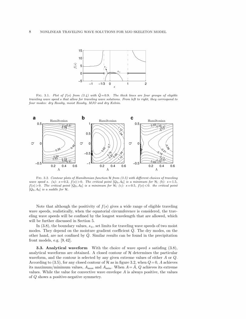
Fig. 3.1. Plot of f(s) from (3.4) with Q= 0.9. The thick lines are four groups of eligibletraveling wave speed s that allow for traveling wave solutions. From left to right, they correspond tofour modes: dry Rossby, moist Rossby, MJO and dry Kelvin.

0.35 0.4

5

0.54

0.63

0.73

0.73

0.82

0.82

0.91

0.91

A

Q

Hamiltonian a

0.2 0.4 0.6−0.5

0

0.5

0.6

2 0.7

0.7

9

0.8

7

0.8

70.9

5

0.9

5

1.0

4

1.0

4

1.0

4

1.1

2

1.1

2

1.1

21

.21

1.2

91

.37

1.4

61

.54

A

Q

Hamiltonian b

0.2 0.4 0.6−1

−0.5

0

0.5

1

−0.4

1−

0.3

6−

0.3

1−

0.2

6

−0.2

6

−0.2

1

−0.21

−0.1

6

−0.16

−0.11

−0.11

−0.07

−0.07

−0.02

−0.02

0.03

0.03

A

Q

Hamiltonian c

0.2 0.4 0.6−0.5

0

0.5

Fig. 3.2. Contour plots of Hamiltonian function H from (3.5) with different choices of travelingwave speed s. (a): s= 0.2, f(s)>0. The critical point [Q0,A0] is a minimum for H; (b): s= 1.5,f(s)>0. The critical point [Q0,A0] is a minimum for H; (c): s= 0.5, f(s)<0. the critical point[Q0,A0] is a saddle for H.

Note that although the positivity of f(s) gives a wide range of eligible travelingwave speeds, realistically, when the equatorial circumference is considered, the trav-eling wave speeds will be confined by the longest wavelength that are allowed, whichwill be further discussed in Section 5.

In (3.8), the boundary values, s±, set limits for traveling wave speeds of two moistmodes. They depend on the moisture gradient coefficient Q. The dry modes, on theother hand, are not confined by Q. Similar results can be found in the precipitationfront models, e.g. [9, 42].

3.3. Analytical waveform With the choice of wave speed s satisfing (3.8),analytical waveforms are obtained. A closed contour of H determines the particularwaveform, and the contour is selected by any given extreme values of either A or Q.According to (3.5), for any closed contour of H as in figure 3.2, when Q= 0, A achievesits maximum/minimum values, Amax and Amin. When A= A, Q achieves its extremevalues. While the value for convective wave envelope A is always positive, the valuesof Q shows a positive-negative symmetry.


When the maximum value of A is selected, the Hamiltonian H is given by (3.5):

H=f(s)

6Γs(HAmax−F logAmax), (3.9)

For other points [Q,A] on the same contour, they satisfy

1

s

[1

2Q2 +

f(s)

6Γ(HA−F logA)

]=f(s)

6Γs(HAmax−F logAmax). (3.10)

According to (3.3b), Q can be replaced by

Q=−sA′

ΓA(3.11)

so that (3.10) becomes an ODE for A:

s2A′2

2Γ2A2+f(s)

6Γ(HA−F logA) =

f(s)

6Γ(HAmax−F logAmax), (3.12)

which can be further written as(dA

dx

)2

=Γf(s)

3s2A2[H(Amax−A)−F (logAmax− logA)

]. (3.13)

This separable ODE has solution in the implicit form:

x=±√

3s2√Γf(s)

∫ Amax

A

a−1[H(Amax− a)−F (logAmax− log a)

]−1/2da+x0 (3.14)

where x=x−st was defined above in (3.1). The integration constant x0 is chosen sothat Amax lies at the center of the domain. Next, from (3.5), Q is derived:

Q(x) =±√f(s)

3Γ

{H[Amax−A(x)]−F [logAmax− logA(x)]

} 12 , (3.15)

where the sign needs to be consistent with (3.3b), depending on the growth/decay ofA and the direction of wave propagation. The other two variables K and R can beobtained by combining (3.2) and (3.3a):

K=− 3s

(1−s)f(s)Q, R=

6s

(1+3s)f(s)Q. (3.16)

The integration constants are chosen to be zero so that K and R have zero meanvalues. Equations (3.14)-(3.16) are the analytical traveling waveform for the nonlinearsystem (1.1).

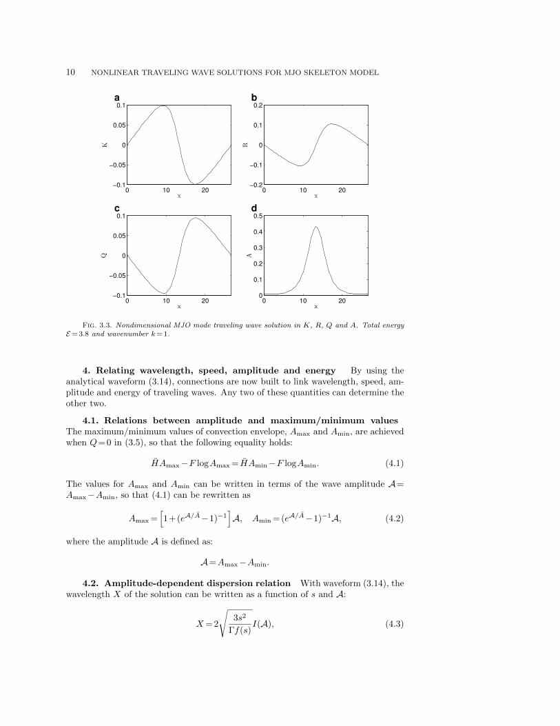
As an initial illustration, an example of an MJO waveform is shown in figure 3.3.The main nonlinear feature is that convective activity A has a pulse-like shape: theregion of enhanced convection is narrower than the region of suppressed convection.At the same time, the positive anomaly is stronger than the negative anomaly (recallfrom (2.10) that the equilibrium value A is 0.1). What remains to be described is howto construct a waveform with certain features specified – e.g., with a wavelength Xthat is a divisor of the Earth’s circumference.


0 10 20−0.1

−0.05

0

0.05

0.1K

a

x0 10 20

−0.2

−0.1

0

0.1

0.2

R

b

x

0 10 20−0.1

−0.05

0

0.05

0.1

Q

x

c

0 10 200

0.1

0.2

0.3

0.4

0.5

A

x

d

Fig. 3.3. Nondimensional MJO mode traveling wave solution in K, R, Q and A. Total energyE= 3.8 and wavenumber k= 1.

4. Relating wavelength, speed, amplitude and energy By using theanalytical waveform (3.14), connections are now built to link wavelength, speed, am-plitude and energy of traveling waves. Any two of these quantities can determine theother two.

4.1. Relations between amplitude and maximum/minimum valuesThe maximum/minimum values of convection envelope, Amax and Amin, are achievedwhen Q= 0 in (3.5), so that the following equality holds:

HAmax−F logAmax = HAmin−F logAmin. (4.1)

The values for Amax and Amin can be written in terms of the wave amplitude A=Amax−Amin, so that (4.1) can be rewritten as

Amax =[1+(eA/A−1)−1

]A, Amin = (eA/A−1)−1A, (4.2)

where the amplitude A is defined as:

A=Amax−Amin.

4.2. Amplitude-dependent dispersion relation With waveform (3.14), thewavelength X of the solution can be written as a function of s and A:

X= 2

√3s2

Γf(s)I(A), (4.3)


−10 −5 0 5 100

5

10

15

wavenumber (2π/40,000 km)

Phase

speed(m

/s)

a

A=0.1A=0.3A=0.5Linear

−10 −5 0 5 100

0.01

0.02

0.03

wavenumber (2π/40,000 km)

Frequency

(cpd)

120 d90 d

60 d

30 d

b

Fig. 4.1. Phase speed s=ω/k (a) and oscillation frequency ω(k) (b) for nonlinear and linearsolutions. Circle: A= 0.1; cross: A= 0.3; square: A= 0.5; star: linear system. The large amplitudephase speeds, i.e. A= 0.5, are 8.76 m/s and 4.61 m/s for k= 1 and 2 equatorial waves. The linearphase speeds, correspondingly, are 10.13 m/s and 5.55 m/s.

where

I(A) =

∫ Amax

Amin

a−1[(H(Amax− a)−F (logAmax− log a)

]−1/2da. (4.4)

The function I(A) illustrates that the wavelength depends on the amplitude A, inaddition to the dependency on wave speeds.

In addition to the amplitude-dependent function (4.3) for the nonlinear waves,a similar function can be derived in the small-amplitude limit for linear waves. Theamplitude dependency on dispersion relation is a nonlinear feature. If the system (1.1)is linearized around A= A, and the traveling wave ansatz is applied, the simplifiedODE system is the linearized (3.3) around A= A,

Q′=f(s)

6sHA

A′=−Γ

sAQ,

(4.5)

where A=A−A. The solution to system (4.5) has wavelength

X= 2π

√6s2

ΓHAf(s)= 2π

√6s2

ΓFf(s), (4.6)

depending on propagation speed s only, in contrast to the wavelength for nonlinearsolutions (4.3), which depends also on wave amplitude A.

Figure 4.1 shows the dimensional phase speed s and oscillation frequency ω(k) =s/k of linear and nonlinear waves for moist Rossby and MJO modes, where thewavenumber k is the number of waves along the 40,000 km long equator. With asmaller amplitude, i.e., A= 0.1, the nonlinear phase speed and oscillation frequencyis almost identical to the linear case. With a larger amplitude, i.e., A= 0.5, due tononlinearity, the phase speed drops and so does the frequency. This analytical re-sult is consistent with two earlier numerical findings. First, a nonlinear numerical


simulation yielded a wave with propagation speed of 6 m/s, in contrast to the linearwave speed of roughly 7 m/s [34]. Second, in the stochastic MJO skeleton model, themaximal spectral power lies at lower frequencies than the linear wave frequency [44];since this holds true even when the stochasticity of the model is reduced (throughtheir parameter ∆a), it suggests that the reduced frequency is likely due to nonlineareffects rather than stochastic effects.

4.3. Total energy of traveling waves Like the wavelength expression in(4.3), the total energy of traveling waves can also be written as a function of s andA. For comparing nonlinear waves of different types (e.g., MJO vs. moist Rossby),the total energy E will be the natural quantity to use.

To derive the total energy of the traveling wave, it is convenient to first introducesome notations. Denote the length of the total domain, here, the nondimensionalequatoriral circumference, as L. The wavenumber k is then k= L

X . The conservedenergy over the whole domain L is the spatial integral of energy density (2.9):

E=k

∫ X

0

[Q

2(1−Q)

(Q

Q−K−R

)2

+K2 +3

2R2 +

H

ΓQA− F

ΓQlogA

]dx (4.7)

With (3.16), the expression is in terms of Q and A only:

E=k

∫ X

0

[g(s)Q2 +

H

ΓQA− F

ΓQlogA

]dx (4.8)

where

g(s) =Q

2(1−Q)

(1

Q− 3s

(s−1)f(s)− 6s

(3s+1)f(s)

)2

+9s2

(s−1)2f2(s)+

54s2

(3s+1)2f2(s)(4.9)

Next, Q can be eliminated through the Hamiltonian function (3.5):

Q2 =f(s)

3Γ

[H(Amax−A)−F (logAmax− logA)

](4.10)

Hence

E=k

∫ X

0

[f(s) g(s)

3Γ

(H(Amax−A)−F (logAmax− logA)

)+H

ΓQA− F

ΓQlogA

]dx

(4.11)Finally, with the implicit solution (3.14), the integration over A replaces the integra-tion over x:

dx

dA=±

√3s2

Γf(s)A−1

[H(Amax−A)−F (logAmax− logA)

]−1/2(4.12)

This allows us to write

E= 2kg(s)

√s2f(s)

3Γ3

∫ Amax

Amin

A−1[H(Amax−A)−F (logAmax− logA)

]1/2dA

+2k

Q

√3s2

f(s)Γ3

∫ Amax

Amin

A−1[H(Amax−A)−F (logAmax− logA)

]−1/2(HA−F logA

)dA

(4.13)


0 5 100

0.2

0.4

0.6

x

ADry Rossby

a

0 5 100

0.2

0.4

0.6

x

A

Moist Rossby b

0 5 100

0.2

0.4

0.6

x

A

MJO c

0 5 100

0.2

0.4

0.6

x

A

Dry Kelvin d

E = 2.5E = 3.0E = 3.5

Fig. 4.2. Figure of A with different total energy E. Wavenumber k= 2.

From (4.3) and (4.13), any two from the following four quantities can determinethe remaining two: traveling speed s, wave amplitude A, wavelength X and totalenergy E . For practical reasons, the wavelength X is usually chosen first so that thecircumference of the equator is a proper domain length.

linear E= 2.5 E= 3.0 E= 3.5Dry Rossby -20.96 -20.87 -20.70 -20.56

Moist Rossby -3.55 -3.51 -3.44 -3.36MJO 5.55 5.39 5.09 4.81

Dry Kelvin 52.30 52.29 52.26 52.24

Table 4.1. Traveling wave speeds (in m s−1) for linear waves and nonlinear waves with differenttotal energy. Wave number k= 2. Corresponding wave structures are shown in figure 4.3.

4.4. Illustrations of waveforms with different amplitudes and energiesWith different wave amplitudes and energies, the waveforms have different shapes dueto nonlinearity. To further illustrate the difference between large and small amplitudesolutions, waveforms with different energies are plotted in figure 4.2, which showsthat, as the energy gets larger (so does the amplitude), the waveforms looks more likea pulse than a sinusoid.

While the shape of waveforms behaves as a nonlinear feature, the relative ratioof variables’ amplitudes does not change much with respect to energy. The ratio is


K R Q A0

0.2

0.4

0.6

0.8

Dry Rossby a

K R Q A0

0.2

0.4

0.6

0.8

Moist Rossby b

K R Q A0

0.2

0.4

0.6

0.8

MJO c

K R Q A0

0.2

0.4

0.6

0.8

Dry Kelvin d

Linear

E=2.5

E=3.0

E=3.5

Fig. 4.3. Contributions of each component A, Q, K and R to the linear and nonlinear travelingwave solutions of four modes: dry Rossby, moist Rossby, MJO and dry Kelvin modes. Results forlinear waves and nonlinear waves with different total energy E= 2.5, 3.0 and 3.5 are shown. Wavenumber k= 2. Corresponding wave speeds are shown in table 4.1.

defined by

K :R :Q :A, (4.14)

where K=Kmax−Kmin and so on. This ratio is analogous to eigenvectors for thelinearized system. In figure 4.3, the ratios are plotted with normalizations by L2-norms of vectors for both nonlinear waveforms with different energies, and linearwaveforms. While the variations for moist Rossby and MJO modes are somewhatvisible, the tendencies for dry modes are hard to see. Another difference betweenmoist and dry modes that can be seen from figure 4.3 is that, moist modes have thedominant contributions from the convective envelope A, yet for the dry modes, thegreatest contributions are from R or K, depending on whether the mode is dry Rossbyor dry Kelvin. The corresponding wave speeds are given in table 4.1.

5. Physical structure In this section, several results are presented in physi-cally relevant terms by returning from the (K,R) variables to the (u,v,θ) variables, byreturning from nondimensional to dimensional units, and by plotting both the zonal(x) and meridional (y) variations.

First, let’s consider the propagation speed s in dimensional units and on a finitedomain. In section 3.2, the allowed propagation speeds s has four branches: dryRossby, moist Rossby, MJO and dry Kelvin waves with the values marked in figure 3.1.From the figure, the traveling wave speed s has a quite large range stretching to infinityfor the two dry modes; in reality, however, the maximum wave speed is confined bytwo facts which can be illustrated from figure 4.1.


0 10 20 30 40−10

−5

0

5

10u(m

/s)

x (1000 km)

a

0 10 20 30 40−1

−0.5

0

0.5

1

θ(K

)

x (1000 km)

b

0 10 20 30 40−0.5

0

0.5

Q(g/kg)

x (1000 km)

c

0 10 20 30 400

1

2

3

4

HA

(K/d)

x (1000 km)

d

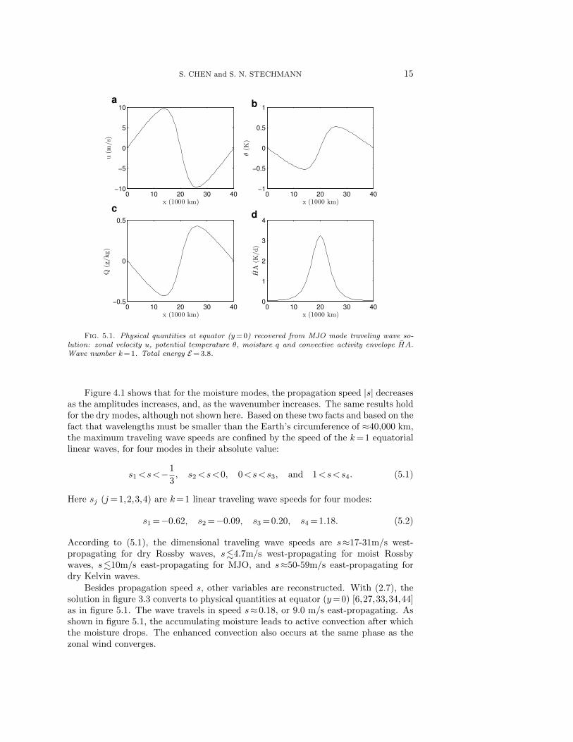
Fig. 5.1. Physical quantities at equator (y= 0) recovered from MJO mode traveling wave so-lution: zonal velocity u, potential temperature θ, moisture q and convective activity envelope HA.Wave number k= 1. Total energy E= 3.8.

Figure 4.1 shows that for the moisture modes, the propagation speed |s| decreasesas the amplitudes increases, and, as the wavenumber increases. The same results holdfor the dry modes, although not shown here. Based on these two facts and based on thefact that wavelengths must be smaller than the Earth’s circumference of ≈40,000 km,the maximum traveling wave speeds are confined by the speed of the k= 1 equatoriallinear waves, for four modes in their absolute value:

s1<s<−1

3, s2<s<0, 0<s<s3, and 1<s<s4. (5.1)

Here sj (j= 1,2,3,4) are k= 1 linear traveling wave speeds for four modes:

s1 =−0.62, s2 =−0.09, s3 = 0.20, s4 = 1.18. (5.2)

According to (5.1), the dimensional traveling wave speeds are s≈17-31m/s west-propagating for dry Rossby waves, s.4.7m/s west-propagating for moist Rossbywaves, s.10m/s east-propagating for MJO, and s≈50-59m/s east-propagating fordry Kelvin waves.

Besides propagation speed s, other variables are reconstructed. With (2.7), thesolution in figure 3.3 converts to physical quantities at equator (y= 0) [6,27,33,34,44]as in figure 5.1. The wave travels in speed s≈0.18, or 9.0 m/s east-propagating. Asshown in figure 5.1, the accumulating moisture leads to active convection after whichthe moisture drops. The enhanced convection also occurs at the same phase as thezonal wind converges.


0 5 10 15 20 25 30 35 40−4

−2

0

2

4

Ha(x, y)− F (K/day) contours

x (1000 km)

y (

1000 k

m)

a

0 5 10 15 20 25 30 35 40−4

−2

0

2

4

q(x, y) (g/kg) contours

x (1000 km)

y (

1000 k

m)

b

0 5 10 15 20 25 30 35 40−4

−2

0

2

4

θ(x, y) (K) contours

x (1000 km)

y (

1000 k

m)

c

Fig. 5.2. MJO mode traveling wave solution. Total energy E= 3.8 and wavenumber k= 1.(a): zonal-meridional structure. Low-level zonal and meridional velocity are shown with contoursof the amplitude of the convective activity envelope. (b): same as (a), except contours of lowertropospheric moisture, q(x,y). (c): same as (a), except contours of lower tropospheric potentialtemperature anomaly, θ. All positive (negative) contours are shown by solid (dashed) lines. Forconvective heating, moisture, and convergence, the contour intervals are 0.55 K/day, 0.15 g/kg,and 0.24 K, respectively. Maximum zonal and meridional velocities are 9.76 m/s and 0.86 m/s,respectively.

With the reconstructed physical variables at equator, the zonal-meridional struc-tures are recovered in figure 5.2 by using the parabolic cylinder functions. One stronglyconvective event is present in this case, collocated with upward vertical motion andhorizontal convergence of the zonal wind. Straddling the equator, a pair of anticy-clones leads and a pair of cyclones trails the convective activity. Also, the maximumlower-troposphere moisture leads the convective maximum. Hence, the nonlinearmodel reproduces the fundamental features of the MJO skeleton model.

In figure 4.2, the pulse-like shape of convection envelope for large amplitude Asuggests that for strong MJO events, the enhanced region is narrower than the sup-pressed region. This is perhaps realistic due to the fact that convective activity


and precipitation are positive quantities and hence have negative anomalies that arebounded. Nevertheless, we are unaware of any observational analysis that definitivelyshows this or even targets this question.

6. Further explorations This section includes preliminary results for severalinteresting topics related to the traveling wave solution for the MJO skeleton model.While the results are not exhaustive, possible directions for future investigations arediscussed.

HA (K/day)

x (1000 km)

t(day

s)

a

0 20 400

20

40

60

80

100

120

140

160

180

200

1 2 3 4

HA (K/day)

x (1000 km)

t(day

s)

b

0 20 400

20

40

60

80

100

120

140

160

180

200

0.5 1 1.5 2

HA (K/day)

x (1000 km)

t(day

s)

c

0 20 400

20

40

60

80

100

120

140

160

180

200

1 2 3

HA (K/day)

x (1000 km)

t(day

s)

d

0 20 400

20

40

60

80

100

120

140

160

180

200

0.5 1 1.5 2

Fig. 6.1. Contours of the amplitude of the convective activity envelope, HA(x,t) at y= 0. (a)-(d) are exact traveling wave solutions for dry Rossby, moist Rossby, MJO and dry Kelvin modeswith total energy E= 3.8.

6.1. Stability vs. instability of traveling wave solutions Analyticaltraveling waveforms to system (1.1) are presented in section 3.3. However, it is unclearhow the waveforms can be affected by perturbations. As a preliminary investigation ofthe stability/instability of waveforms, we perform numerical computations for (1.1),by adopting the scheme from [34], where an operator splitting method is used toseparate the linear part (1.1a)-(1.1c) and nonlinear part (1.1d).

First, the numerical integrations are initialized with analytical waveforms[Ke,Re,Qe,Ae] given by (3.14)-(3.16). Tests are run up to T = 200 days with twoenergies for four modes: E= 2.5 and E= 3.8. Although cases with two energies wereperformed, only results of E= 3.8 cases are shown as contour plots of convective ac-tivity envelope HA(x,t) in figure 6.1. In the figure, the parallel lines are exhibitedfor most of the plots, indicating that the numerical nonlinear wave is propagating ata fixed speed.

Next, perturbations are placed on the initial waveforms. The perturbed initialcondition is written as

[K,R,Q,A] = [Ke,Re,Qe,Ae]+[K ′,R′,Q′,A′], (6.1)


where the perturbation [K ′,R′,Q′,A′] are Gaussian functions scaled by 10% of eachvariable’s maximum values,

[K ′,R′,Q′,A′] =1

10exp(−x

2

16)[Kmax,Rmax,Qmax,Amax], (6.2)

and they decay fast enough so that the periodicity of the initial condition is notaffected.

The numerical integrations are then performed (not shown) with perturbed initialdata (6.1) up to T = 200 days. To evaluate the effect of perturbations, the quantity“pattern correlation” P is used, which is defined by

P(t)[Ae,A] =

∫Ae(x,t)A(x,t)dx

||Ae(x,t)||2||A(x,t)||2, (6.3)

where Ae(x,t) and A(x,t) are exact solutions and perturbed solutions. From (6.3), itcan be seen that the extreme values of P are ±1, achieved when A(x,t) =CAe(x,t),for which the sign of C determines whether it is a maximum or a minimum. Theproximity of P to the maximum value 1 indicates the perturbation has little impact,thus the solution is stable.

Two cases with total energy E= 2.5 and E= 3.8 are performed here, with initialconditions described in (6.1). For traveling waves with total energy E= 2.5, the pat-tern correlation P(t)≥97% up to T = 200 days for all modes. The number 97% isclose to 1, implying only a slight effect of the perturbation. In the other case, fortraveling waves with total energy E= 3.8, solutions are quite unstable based on thepattern correlation except for the moist Rossby mode, holding a pattern correlationgreater than 97% up to T = 200 days. For other three modes, the values of P dropsignificantly within the computational time. To identify a great impact from the per-turbation, the threshold 90% is used here: when the pattern correlation P<90%,the data is greatly affected by the initial perturbation. For the other three modes,dry Rossby mode is the first to have P(t)<90%, appearing at T = 62 day; MJO anddry Kelvin mode have the first P(t)<90% around T = 130 day. From the numericalexperiment performed, it may suggest that the moist Rossby mode is most stable, butno firm conclusion can be drawn based on numerical experiment alone.

6.2. The weak-forcing limit and sech-squared waveforms In section 3.3,the nonlinear traveling wave solution is given implicitly in terms of an integral for thecase of finite forcing, F . In this section, the forcing term, F , is taken to be vanishing,i.e., F→0. We show now that, in the limiting case, the solution is a solitary wavewhose waveform in the function sech2. According to (4.2),

Amax→A, Amin→0, as F→0. (6.4)

Also note that in the integral equation (3.13), the function on the right-hand-side hasthe asymptotic behavior that

A2[H(A−A)−F (logA− logA)

]∼ HA2(A−A), as F→0. (6.5)

Under this limit, equation (3.13) becomes

A′=±√

ΓHf(s)

3s2A√A−A (6.6)


With writing

h(s) =

√ΓHf(s)

3s2, (6.7)

the solution turns out to be

A(x) =A sech2

[1

2h(s)√A (x−x0)

], (6.8)

where x0 is an integration constant that determines the location ofA. This integrationprocedure is similar to get a soliton from KdV equation.

In the solution (6.8), the wavelength goes to infinity as the forcing term vanishes,i.e., F→0. Besides wavelength, another important length scale is the effective widthof A, or namely, the length of enhanced convective region, d, which is defined as

d=1

h(s)√A. (6.9)

The effective width d is determined by both the wave amplitude A, and the wavespeed s.

6.3. The model without meridional (y) variations The model (1.2) ne-glects meridional (y) variation and can be considered as the atmospheric circulationdirectly above the equator, y= 0, where the Coriolis force is negligible. Similar resultshold equally well for (1.2) and (1.1). While (1.2) neglects important physics, theireast-west symmetry simplifies the mathematical formulas. The model (1.2) wouldperhaps be easier to study in regard to the further questions raised in sections 6.1and 6.2.

The key results of traveling wave solutions are provided for system (1.2). With thetraveling wave ansatz x=x−st, system (1.2) is reduced to the nonlinear oscillatoryODE:

Q′=1

s(

1− Q1−s2

) (HA−F ) (6.10a)

A′=−Γ

sAQ (6.10b)

The Hamiltonian function of (6.10) writes:

H(Q,A) =1

s

[Γ

2Q2 +

1−s2

1−s2−Q(HA−F logA)

]. (6.11)

The solution existence requires that H has closed contours, which turn out to be:

1−s2

s2(1−s2−Q)>0, (6.12)

or equivalently,

s2>1 or 0<s2<1−Q. (6.13)

Unlike the system (1.1), the allowed wave propagation speed s for (1.2) has east-westsymmetry. Here, the limiting values for dry waves and moist waves are

cdry = 1, and cmoist =

√1−Q. (6.14)


These critical values are the same in the model governing precipitation fronts [9, 42],where traveling speed boundaries were set for drying fronts, slow moistening frontsand fast moistening fronts. Given (6.10)-(6.14), one can derive results analogous tothose presented in section 3.

7. Conclusions Nonlinear traveling wave solutions were presented for theMJO skeleton model, and they were compared with their linear counterparts. Thenonlinear traveling waves come in four types, and the propagation speed of each typeis restricted to lie in a particular interval. One wave type has a structure and sloweastward propagation speed that are consistent with the MJO. In the nonlinear MJOwave, the convective activity has a pulse-like shape, with a narrow region of enhancedconvection and a wide region of suppressed convection. Furthermore, an amplitude-dependent dispersion relation was derived, and it shows that the nonlinear MJO hasa lower frequency and slower propagation speed than the linear MJO. By takingthe small-amplitude limit, an analytic formula was also derived for the dispersionrelation of linear waves. To derive all of these results, a key aspect was the model’sconservation of energy, which holds even in the presence of the forcing term, F .

The results here suggest several interesting directions for observational analysisof the MJO. In particular, What are the amplitude-dependent properties of the MJOin observational data? As one example, for large-amplitude MJO events, is the re-gion of enhanced convection stronger and/or narrower than the region of suppressedconvection? An affirmative answer would perhaps be expected due to the simplefact that convective activity and precipitation are positive quantities (as illustratedhere in figure 4.2). Nevertheless, we are unaware of any observational analysis thatdefinitively shows this or even targets this question. In some numerical simulationsof the MJO [1,17], it appears to the eye that such an asymmetry might exist betweenenhanced and suppressed convection regions.

Another interesting direction is to investigate the stability of the nonlinear waves.In our numerical simulations, all nonlinear wave types can be reproduced and canpropagate around the Earth’s circumference a dozen or more times with very littlechange to their structure. When perturbed, the numerical waves still retain a sig-nificant amount of their coherent propagation, although some wave modulation canarise, and it can be difficult to know for certain which perturbed features are partof the true variability and which are numerical artifacts. It would be interesting torigorously prove the stability or instability of the nonlinear waves.

Finally, another open question is whether the MJO skeleton model is possiblya completely integrable system. The nonlinearity has a mathematical form that isreminiscent of the Toda lattice model [45, 46] when written in terms of Flaschka’svariables [8]. Perhaps one could expand upon this similarity. The mathematicallysimplest case to consider is probably the weak-forcing limit F→0 on the real line,rather than the physically realistic case of finite forcing F 6= 0 on a periodic domain.In the limit of weak forcing, it was shown that the shape of the nonlinear travelingwaves is greatly simplified and has a simple sech2 waveform, the same form as thesoliton of the KdV equation.

Acknowledgement. The authors thank A. Majda for helpful discussions. Theresearch of S.N.S. is partially supported by the ONR Young Investigator Programthrough grant N00014-21-1-0744 and by the ONR-MURI grant N00014-12-1-0912.S.C. is supported as a postdoctoral researcher on grant ONR-MURI N00014-12-1-0912.


REFERENCES

[1] R. S. Ajayamohan, B. Khouider, and A. J. Majda, Realistic initiation and dynamics of theMadden–Julian Oscillation in a coarse resolution aquaplanet GCM, Geophys. Res. Lett.,40 (2013), pp. 6252–6257.

[2] J. Benedict and D. Randall, Structure of the Madden-Julian Oscillation in the Superpa-rameterized CAM, J. Atmos. Sci., 66 (2009), pp. 3277–3296.

[3] J. A. Biello, Nonlinearly coupled KdV equations describing the interaction of equatorial andmidlatitude Rossby waves, Chinese Annals of Mathematics, Series B, 30 (2009), pp. 483–504.

[4] J. A. Biello and A. J. Majda, The effect of meridional and vertical shear on the interactionof equatorial baroclinic and barotropic Rossby waves, Studies in Applied Mathematics, 112(2004), pp. 341–390.

[5] J. A. Biello and A. J. Majda, A new multiscale model for the Madden–Julian oscillation.,J. Atmos. Sci., 62 (2005), pp. 1694–1721.

[6] , Modulating synoptic scale convective activity and boundary layer dissipation in theIPESD models of the Madden–Julian oscillation, Dyn. Atmos. Oceans, 42 (2006), pp. 152–215.

[7] J. Dias, S. Leroux, S. N. Tulich, and G. N. Kiladis, How systematic is organized tropicalconvection within the MJO?, Geophys. Res. Lett, 40 (2013), pp. 1420–1425.

[8] H. Flaschka, The Toda lattice. II. Existence of integrals, Phys. Rev. B, 9 (1974), pp. 1924–1925.

[9] D. M. W. Frierson, A. J. Majda, and O. M. Pauluis, Large scale dynamics of precipitationfronts in the tropical atmosphere: a novel relaxation limit, Commun. Math. Sci., 2 (2004),pp. 591–626.

[10] A. E. Gill, Atmosphere–Ocean Dynamics, vol. 30 of International Geophysics Series, AcademicPress, 1982.

[11] G. Gottwald and R. Grimshaw, The effect of topography on the dynamics of interactingsolitary waves in the context of atmospheric blocking, J. Atmos. Sci., 56 (1999), pp. 3663–3678.

[12] W. W. Grabowski, MJO-like coherent structures: sensitivity simulations using the cloud-resolving convection parameterization (CRCP)., J. Atmos. Sci., 60 (2003), pp. 847–864.

[13] Y. Guo, K. Simon, and E. S. Titi, Global well-posedness of a system of nonlinearly coupledKdV equations of Majda and Biello, arXiv preprint arXiv:1310.1130, (2013).

[14] H. H. Hendon and B. Liebmann, Organization of convection within the Madden–Julian os-cillation, J. Geophys. Res., 99 (1994), pp. 8073–8084.

[15] B. Khouider, Y. Han, A. J. Majda, and S. N. Stechmann, Multiscale waves in an MJO back-ground and convective momentum transport feedback, J. Atmos. Sci., 69 (2012), pp. 915–933.

[16] B. Khouider, A. J. Majda, and S. N. Stechmann, Climate science in the tropics: waves,vortices and PDEs, Nonlinearity, 26 (2013), pp. R1–R68.

[17] B. Khouider, A. St-Cyr, A. J. Majda, and J. Tribbia, The MJO and convectively coupledwaves in a coarse-resolution GCM with a simple multicloud parameterization, J. Atmos.Sci., 68 (2011), pp. 240–264.

[18] D. Kim, K. Sperber, W. Stern, D. Waliser, I.-S. Kang, E. Maloney, W. Wang, K. We-ickmann, J. Benedict, M. Khairoutdinov, et al., Application of MJO simulation di-agnostics to climate models, J. Climate, 22 (2009), pp. 6413–6436.

[19] R. Klein, Scale-dependent models for atmospheric flows, Annu. Rev. Fluid Mech., 42 (2010),pp. 249–274.

[20] B. J.-F. L. J. Kouznetsov, D. and K. Ueda, Self-pulsing laser as oscillator toda: approxima-tions through elementary functions, J. Phys, A: Math. Theor., 40 (2007), pp. 2107–2124.

[21] W. K. M. Lau and D. E. Waliser, eds., Intraseasonal Variability in the Atmosphere–OceanClimate System, Springer, Berlin, 2012.

[22] d. V.-S. M. v. E. M. P. Lien, Y. and J. P. Woerdman, Lasers as toda oscillators, J. Opt.Soc. Am. B, 19 (2002), pp. 1461–1466.

[23] J.-L. Lin, G. N. Kiladis, B. E. Mapes, K. M. Weickmann, K. R. Sperber, W. Lin,M. Wheeler, S. D. Schubert, A. Del Genio, L. J. Donner, S. Emori, J.-F. Gueremy,F. Hourdin, P. J. Rasch, E. Roeckner, and J. F. Scinocca, Tropical intraseasonalvariability in 14 IPCC AR4 climate models Part I: Convective signals, J. Climate, 19(2006), pp. 2665–2690.

[24] R. A. Madden and P. R. Julian, Detection of a 40–50 day oscillation in the zonal wind inthe tropical Pacific, J. Atmos. Sci., 28 (1971), pp. 702–708.


[25] , Description of global-scale circulation cells in the Tropics with a 40–50 day period., J.Atmos. Sci., 29 (1972), pp. 1109–1123.

[26] , Observations of the 40–50-day tropical oscillation—a review, Mon. Wea. Rev., 122(1994), pp. 814–837.

[27] A. J. Majda, Introduction to PDEs and Waves for the Atmosphere and Ocean, vol. 9 ofCourant Lecture Notes in Mathematics, American Mathematical Society, Providence, 2003.

[28] A. J. Majda and J. A. Biello, The nonlinear interaction of barotropic and equatorial baro-clinic Rossby waves., J. Atmos. Sci., 60 (2003), pp. 1809–1821.

[29] , A multiscale model for the intraseasonal oscillation, Proc. Natl. Acad. Sci. USA, 101(2004), pp. 4736–4741.

[30] A. J. Majda and R. Klein, Systematic multiscale models for the Tropics., J. Atmos. Sci., 60(2003), pp. 393–408.

[31] A. J. Majda and P. E. Souganidis, Existence and uniqueness of weak solutions for precipi-tation fronts: A novel hyperbolic free boundary problem in several space variables, Comm.Pure Appl. Math., 63 (2010), pp. 1351–1361.

[32] A. J. Majda and S. N. Stechmann, A simple dynamical model with features of convectivemomentum transport, J. Atmos. Sci., 66 (2009), pp. 373–392.

[33] , The skeleton of tropical intraseasonal oscillations, Proc. Natl. Acad. Sci. USA, 106(2009), pp. 8417–8422.

[34] , Nonlinear dynamics and regional variations in the MJO skeleton, J. Atmos. Sci., 68(2011), pp. 3053–3071.

[35] H. Mitsudera, Eady solitary waves: a theory of type b cyclogenesis, J. Atmos. Sci., 51 (1994),pp. 3137–3154.

[36] M. W. Moncrieff, The multiscale organization of moist convection and the intersection ofweather and climate, in Climate Dynamics: Why Does Climate Vary?, D.-Z. Sun andF. Bryan, eds., vol. 189 of Geophysical Monograph Series, American Geophysical Union,Washington, D. C., 2010, pp. 3–26.

[37] M. W. Moncrieff and E. Klinker, Organized convective systems in the tropical westernPacific as a process in general circulation models: a TOGA COARE case-study, Q. J.Roy. Met. Soc., 123 (1997), pp. 805–827.

[38] T. Nakazawa, Tropical super clusters within intraseasonal variations over the western Pacific,J. Met. Soc. Japan, 66 (1988), pp. 823–839.

[39] T. Oh, Invariant Gibbs measures and as global well posedness for coupled KdV systems, Dif-ferential and Integral Equations, 22 (2009), pp. 637–668.

[40] G. L. Oppo and A. Politi, Toda potential in laser equations, Z. Phys. B – Condensed Matter,59 (1985), pp. 111–115.

[41] J. M. Slingo, K. R. Sperber, J. S. Boyle, J.-P. Ceron, M. Dix, B. Dugas, W. Ebisuzaki,J. Fyfe, D. Gregory, J.-F. Gueremy, J. Hack, A. Harzallah, P. Inness, A. Kitoh,W. K.-M. Lau, B. McAvaney, R. Madden, A. Matthews, T. N. Palmer, C.-K. Park,D. Randall, and N. Renno, Intraseasonal oscillations in 15 atmospheric general cir-culation models: results from an AMIP diagnostic subproject, Climate Dyn., 12 (1996),pp. 325–357.

[42] S. N. Stechmann and A. J. Majda, The structure of precipitation fronts for finite relaxationtime, Theor. Comp. Fluid Dyn., 20 (2006), pp. 377–404.

[43] S. N. Stechmann, A. J. Majda, and D. Skjorshammer, Convectively coupled wave–environment interactions, Theor. Comp. Fluid Dyn., 27 (2013), pp. 513–532.

[44] S. Thual, A. J. Majda, and S. N. Stechmann, A stochastic skeleton model for the MJO, J.Atmos. Sci., 71 (2014), pp. 697–715.

[45] M. Toda, Vibration of a chain with nonlinear interaction, J. Phys. Soc. Japan, 22 (1967),pp. 431–436.

[46] M. Toda, Studies of a non-linear lattice, Physics Reports, 18 (1975), pp. 1–123.[47] C. Zhang, Madden–Julian Oscillation, Reviews of Geophysics, 43 (2005), p. RG2003.

NONLINEAR TRAVELING WAVES FOR THE SKELETON …stechmann/publications/ChenStechmann2016... ·...

Documents

Transcript of NONLINEAR TRAVELING WAVES FOR THE SKELETON …stechmann/publications/ChenStechmann2016... ·...