Nonlinear optimization tool for the analysis of the

manoeuvre capability of a submarine

Javier Garcıa, Diana Ovalle, and Francisco Periago,

J. Garcıa is with the Direction of Engineering, DICA, Navantia S. A., Cartagena, 30205, Spain.

D. Ovalle is with the Department of Applied Mathematics and Statistics, ETSI Industriales, Universidad Politecnica de Cartagena, Cartagena,

30202, Spain. Phone: (968) 33-8948, email: diana.ovalle@upct.es.Supported by projects 2113/07MAE from Navantia S. A. and 08720/PI/08

from Fundacion Seneca, Agencia de Ciencia y Tecnologıa de la Region de Murcia (Programa de Generacion de Conocimiento Cientıfico de

Excelencia, IIPCTRM 2007-10).

F. Periago is with the Department of Applied Mathematics and Statistics, ETSI Industriales, Universidad Politecnica de Cartagena,

Cartagena, 30202, Spain. Phone: (968) 33-8909, email: f.periago@upct.es. Supported by projects MTM2007-62945 from Ministerio de

Ciencia y Tecnologıa (Spain), 08720/PI/08 from Fundacion Seneca, Agencia de Ciencia y Tecnologıa de la Region de Murcia (Programa de

Generacion de Conocimiento Cientıfico de Excelencia, IIPCTRM 2007-10) and 21131/07MAE from Navantia S.A.

1

Nonlinear optimization tool for the analysis of the

manoeuvre capability of a submarine

Abstract

A six degree of freedom (6-DOF) highly nonlinear and coupledmathematical model for the equation of motion

of a manned submarine is proposed. In order to analyze some specific manoeuvre capabilities of the underwater

vehicle, we formulate an unconstrained optimal control problem which has this system of ordinary differential

equations as the underlying state law. Then, we solve numerically the optimization problem by using a gradient

descent method. We pay special attention to the analysis of the numerical difficulties inherent to the model.

Simulation results are presented and analyzed for two givenmanoeuvres, where we compare the results with a

typical linear model to highlight the effects of coupling inour model. We emphasize that the mathematical model

and the optimization algorithm proposed in this work may be useful to: (a) help designers in the preliminary

state design of a submarine, and (b) as a guidance system, in the sense it provides a set of admissible (and in a

certain optimal sense) set of trajectories to be used in the design of controllers based on trajectory-tracking and/or

path-following.

Index Terms

Gradient descent method, numerical simulations, optimal control theory, submarine manoeuvrability, trajectories

generation.

I. I NTRODUCTION

DURING the last decades there have been many studies about underwater vehicles, mainly address-

ing autonomous underwater vehicles (AUVs) or Remote Operated Vehicles (ROVs), which are

”small” vehicles, normally unmanned, designed for specifical purposes and useful in mamy applications

([1], [2], and the references there in). Nevertheless, for big submarines normally designed for military

purposes, manned, with weight from1000 to 10000 tons and length around60 to 100 meters, since the

2

publication of their dynamic models by the David Taylor Naval Ship Research and Development Center

[3], not so much have been done (mainly because of confidentiality).

The needs of manoeuvrability in these submarines are quite different from the ones in AUVs or ROVs.

In particular, they should be able to avoid torpedoes which implies change their course or their depth

fast, to navigate in littoral waters which implies maintenance accurate the depth during a turning, to be

undetectable which implies low noise generation when manoeuvring and to remain underwater as long as

possible. Checking those qualities for selling a design could be done by numerical or physical simulations,

as long as the costumer were satisfied with the results.

Generally, studies and tests on underwater vehicles manoeuvre capability are performed by numerical

simulation of linear or nonlinear mathematical models, which normally have no coupling, ([4], [5], [6]).

Nevertheless, the results from this work show that the submarine movement is highly coupled in all its

planes and it should not be realistic to neglect those couplings in certain applications, mainly in those

showing the submarine behavior, that is, results from implementation of controllers, observers, etc...

Normally, one do not make open loop analysis of a system. But inour case, since we want to analyze the

submarine manoeuvre capability, it is really useful. It is here where the controllability theory starts to play

an important part in this work, in the sense that we want to know how to move the submarine control

surfaces to achieve a manoeuvre in an optimal sense. Here a manoeuvre is considered as a particular

movement which allows the submarine to satisfy the above mentioned needs of manoeuvrability. For us,

the crucial manoeuvre capabilities are:

• Turning ability,

• fast course and depth changes, and

• moderate vertical movements, especially to avoid large depth excursions in case of an aft planes jam.

In this respect, it is also important to notice that althoughour design requirements clearly define an

ocean vehicle, however, some of the missions are within the littoral scenario and due to the size of

the vehicle they are very restricted waters.

3

In order to be able to analize these capabilities, a first stepis to have an accurate mathematical model

for the equations of motion, and second, a suitable optimization strategy.

Concerning to the mathematical model for the equations of motion, taking as a starting point the

standard DTNSRDC nonlinear equations of motion for an underwater vehicle (see [3], [7], [8]), taking

into account the particularities of marine hydrodynamics (see [9]), and adapting these general equations to

the particular characteristics of a prototype developed bythe company Navantia S.A. Cartagena Shipyard

(Spain), we propose a mathematical model composed of a highly coupled and nonlinear system of ordinary

differential equations (ODEs) with six degrees of freedom.For comparison reasons, we also will consider

a simplified linear model. The values of the hydrodynamic coefficients which appear in the equations of

both models (linear and nonlinear) have been experimentally obtained by using a scale model.

Above we stated that controllability theory plays an important part of the work. Nevertheless, for the

nonlinear case, the mathematical controllability theory is not sufficiently developed for the case in which

controls appear in nonlinear form, which is our case. For this reason, we propose to formulate the problem

as an unconstrained optimal control problem in which the cost to be minimized is a commitment between

reaching the final desired state at a fixed time (this is important because we are analyzing manoeuvre

capability) and a minimum use of controls. The approach we pursue in this paper for the nonlinear case

is the natural extension of the linear controllability theory.

Next, we would like to comment about the numerical method we propose to solve our nonlinear

optimal control problem. As usual in this context, we implement a gradient descent method. It requires

the resolution, at each iteration, of the state law (18) and the system for the adjoint state (19). Since

the state equation includes non-differentiable functionslike the absolute value and squared roots, the

right-hand side of the adjoint equation is discontinuous. This is a very delicate issue which historically

motivated the development of differential inclusions [10]. Uniqueness of solutions for the corresponding

problem is typically lost and therefore the numerical method for solving the adjoint equation should be

able to capture the physically admissible solution. As we will see later on, a transversality condition on

4

the hypersurface of discontinuity must be satisfied. We do believe that it is really important to analyze in

detail these mathematical difficulties.

At the end, the numerical simulation results obtained with our methodology could be useful as a

guidance system, in the sense that we provide a set of trajectories for the state variables with the important

characteristic of been feasible for the submarine. Even, from those trajectories one can eliminate time in

the final results and provide paths independent of time, in function of any variable of interest. Then, these

results might be used in the design of controllers based on tracking-trajectory and/or path-following.

The rest of the paper is organized as follows. In Section 2, webriefly describe the kinematic and

dynamic equations of motion for our model. Section 3 proposes a simplified linear version of those

equations and reviews on the use of controllability theory for solving the control problem. In Section 4

we formulate our control problem as an unconstrained optimal control problem and describe a gradient

descent method for solving it. We pay special attention on the analysis of the mathematical difficulties

inherent to it. Finally, Section 5 is devoted to numerical simulation of a set of standard manoeuvres which

are commonly used by designers at the preliminary design state.

II. V EHICLE MODELING

The three-dimensional equations of motion for an underwater vehicle are usually described by using

two coordinate frames: the moving coordinate frame which isfixed to the vehicle and is called thebody-

fixed reference frame, and the earth-fixed reference frame which is called theworld reference frame. The

position and orientation of the vehicle are described in theworld system while the linear and angular

velocities are expressed in the body-fixed coordinate system. These quantities are defined according to

SNAME notation [7] as:

η (t) =[ηT

1 (t) , ηT2 (t)

], η1 (t) = [x (t) , y (t) , z (t)]T , η2 (t) = [φ (t) , θ (t) , ψ (t)]T

ν (t) =[νT

1 (t) , νT2 (t)

], ν1 = [u (t) , v (t) , w (t)]T , ν2 (t) = [p (t) , q (t) , r (t)]T .

(1)

5

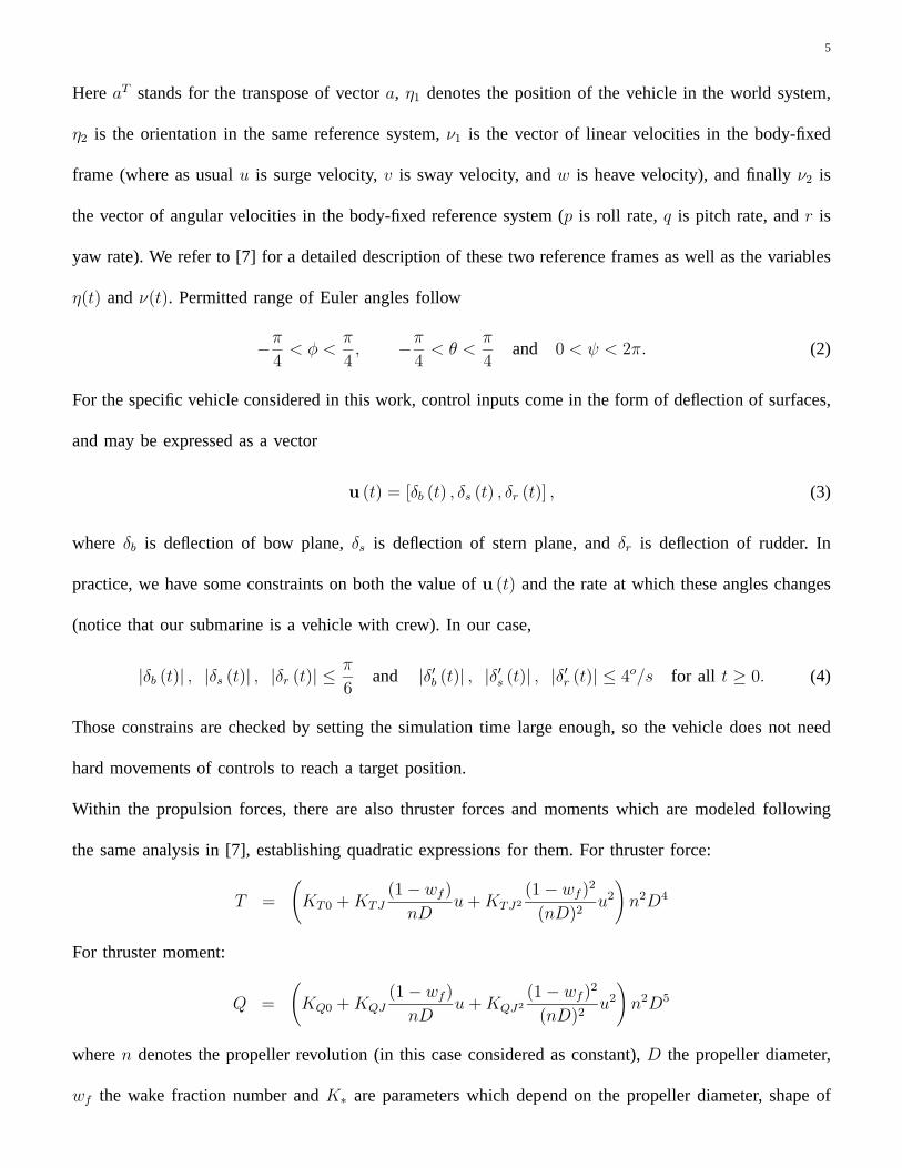
HereaT stands for the transpose of vectora, η1 denotes the position of the vehicle in the world system,

η2 is the orientation in the same reference system,ν1 is the vector of linear velocities in the body-fixed

frame (where as usualu is surge velocity,v is sway velocity, andw is heave velocity), and finallyν2 is

the vector of angular velocities in the body-fixed referencesystem (p is roll rate,q is pitch rate, andr is

yaw rate). We refer to [7] for a detailed description of thesetwo reference frames as well as the variables

η(t) andν(t). Permitted range of Euler angles follow

−π4< φ <

π

4, −π

4< θ <

π

4and 0 < ψ < 2π. (2)

For the specific vehicle considered in this work, control inputs come in the form of deflection of surfaces,

and may be expressed as a vector

u (t) = [δb (t) , δs (t) , δr (t)] , (3)

where δb is deflection of bow plane,δs is deflection of stern plane, andδr is deflection of rudder. In

practice, we have some constraints on both the value ofu (t) and the rate at which these angles changes

(notice that our submarine is a vehicle with crew). In our case,

|δb (t)| , |δs (t)| , |δr (t)| ≤ π

6and |δ′b (t)| , |δ′s (t)| , |δ′r (t)| ≤ 4o/s for all t ≥ 0. (4)

Those constrains are checked by setting the simulation timelarge enough, so the vehicle does not need

hard movements of controls to reach a target position.

Within the propulsion forces, there are also thruster forces and moments which are modeled following

the same analysis in [7], establishing quadratic expressions for them. For thruster force:

T =

(KT0 +KTJ

(1 − wf )

nDu+KTJ2

(1 − wf )2

(nD)2u2

)n2D4

For thruster moment:

Q =

(KQ0 +KQJ

(1 − wf )

nDu+KQJ2

(1 − wf )2

(nD)2u2

)n2D5

wheren denotes the propeller revolution (in this case considered as constant),D the propeller diameter,

wf the wake fraction number andK∗ are parameters which depend on the propeller diameter, shape of

6

the duct, water density, etc. Those models for thruster force and moment are valid forn ≥ 0 and vary in

function of the submarine forward velocity,u.

The vehicle motion is described as a system of twelve (six kinematic + six dynamic) nonlinear ordinary

differential equations. Following the conventional notation

η = J(η)ν (5)

Mν + C(ν)ν + D(ν)ν + f(η) = τu + τT (6)

Following [7], [11]:

J(η) =

J1 (η2) 03×3

03×3 J2 (η2)

, (7)

with

J1 (η2) =

cosψ cos θ − sinψ cos θ + cosψ sin θ sinφ sinψ sinφ+ cosψ cosφ sin θ

sinψ cos θ cosψ cosφ+ sinφ sin θ sinψ − cosψ sinφ+ sin θ sinψ cosφ

− sin θ cos θ sinφ cos θ cosφ

and

J2 (η2) =

1 sinφ tan θ cosφ tan θ

0 cosφ − sinφ

0 sinφ/ cos θ cosφ/ cos θ

.

For the dynamic equation (6)

M , MRB + MA and C(ν) , CRB(ν) + CA(ν)

where,MRB is the rigid-body inertia matrix,CRB(ν) is the rigid-body Coriolis and Centripetal matrix,

MA is the added inertia matrix andCA(ν) is a matrix of hydrodynamic Coriolis and Centripetal terms

due to added mass.D(ν) represents hydrodynamic damping due to vortex shedding andskin friction,

g(η) represent the restoring forces,τ are propulsion forces due to control surfaces movement andτT are

7

propulsion forces due to the propeller. The specific expressions for those matrices are

MRB =

m 0 0 0 mzG −myG

0 m 0 −mzG 0 mxG

0 0 m myG −mxG 0

0 −mzG myG Ix −Ixy −Izx

mzG 0 −mxG −Ixy Iy −Iyz

−myG mxG 0 −Izx −Iyz Iz

CRB(ν) =

0 −mr mq m(yGq + zGr) −mxGq −mxGr

mr 0 −mp −myGp m(zGr + xGp) −myGr

−mq mp 0 −mzGp −mzGq m(xGp + yGq)

−m(yGq + zGr) myGp mzGp 0 −(Ixzp + Iyzq) + Izr Ixyp + Iyzr − Iyq

mxGq −m(zGr + xGp) mzGq Ixzp + Iyzq − Izr 0 −(Ixyq + Izxr) − Ixp

mxGr −myGr −m(xGp + yGq) −(Ixyp + Iyzr) − Iyq Ixyq + Izxr − Ixp 0

MA =

X ′u 0 0 0 0 0

0 Y ′v 0 lY ′

p 0 lY ′r

0 0 Z ′w 0 lZ ′

q 0

0 lK ′v 0 lK ′

p 0 lK ′r

0 0 lM ′w 0 lM ′

q 0

0 lN ′v 0 lN ′

p 0 lN ′r

CA(ν) =

0 0 0 0 X ′qqq +X ′

wqw X ′rrr +X ′

vrv +X ′rpp

0 0 0 Y ′pu+ Y ′

pqq Y ′wpw Y ′

ru

0 0 0 Z ′vpv Z ′

qu 0

0 K ′vu K ′

wpp 0 K ′qrr K ′

ru

M ′qq +M ′

ww 0 M ′vwv M ′

rpr 0 M ′vrv +M ′

rrr

N ′rr N ′

vu 0 N ′pu N ′

pqp 0

8

D(ν) =

X ′uuu X ′

vvv X ′www +X ′

w|w||w| 0 X ′q|q||q| 0

Y ′vv Y ′

v|v|

√v2 + w2 0 0 0 Y ′

r|r||r|

Z ′|w||w| + Z ′

ww Z ′vrr + Z ′

vvv 0 0 Z ′q|q||q| Z ′

rrr

K ′pu K ′

v|v||v| 0 K ′p|p||p| 0 K ′

r|r||r|

M ′|w||w| M ′

vvv M ′w|w|

√v2 + w2 0 M ′

q|q||q| 0

0 N ′v|v|

√v2 + w2 0 0 0 N ′

r|r||r|

g(η) =

(W −B) sin(θ)

−(W −B) cos(θ) sin(φ)

−(W −B) cos(θ) cos(φ)

−(yGW − yBB) cos(θ) cos(φ) + (zGW − zBB) cos(θ) sin(φ)

(zGW − zBB) sin(θ) + (xGW − xBB) cos(θ) cos(φ)

−(xGW − xBB) cos(θ) sin(φ) − (yGW − yBB) sin(θ)

τ =ρ

2l2u2

X ′δrδr

δr X ′δsδs

δs X ′δbδb

δb

Y ′δr

+ Y ′δrη

(η − 1

C

)C 0 0

0 Z ′δs

+ Z ′δsη

(η − 1

C

)C Z ′

δb

lK ′δr

0 0

0 l[M ′

δs+M ′

δsη

(η − 1

C

)C]

lM ′δb

l[N ′

δr+ Y ′

δrη

(η − 1

C

)C]

0 0

τT = ρ

[

T (1 − t) 0 0 −Q 0 0

]T

In the definition of the above matrices, we can see the coupling between the movements on the different

planes, but mainly inD(ν). The works about AUVs and ROVs takeD(ν) as a diagonal matrix, which

for the purposes following in each work is useful, but in thiswork we want to see the effects of that

coupling.

9

For convenience, we rewrite the system defined by (5) and (6) as follows

E·x= f (x (t) ,u (t)) (8)

where

x (t) = [x (t) , y (t) , z (t) , φ (t) , θ (t) , ψ (t) , u (t) , v (t) , w (t) , p (t) , q (t) , r (t)] . (9)

and

E =

I6×6 06×6

06×6 M

.

SinceE is invertible, (8) transforms into the more usual form

·x (t) = f (x (t) ,u (t)) (10)

wheref = E−1f .

Specific values of the particular hydrodynamic coefficientswhich appear in the equations depend on

the specific vehicle and, therefore, would require modification if applied to other vehicles. The values of

the coefficients used in this work have been experimentally obtained in deeply submerged conditions by

using the scale model showed in Fig. 1 and are listed in Appendix.

From a pure mathematical point of view, it is important to point out the following facts in the proposed

model:

• The high nonlinear character of the equations and the high order of the system (12 equations).

• The lack of differentiability of the system which is caused for several terms involving non-differentiable

functions such as the absolute value and squared roots.

• Controls appear in nonlinear (quadratic) form.

III. A LINEAR MODEL

The material of this section has been essentially taken from[12], but for the sake of completeness we

include it here. Taking as a starting point the set of equations (5) and (6) with the corresponding matrices

definition, and making the additional assumptions:

10

• constant surge velocityu0,

• deeply submerged conditions,

• small variations in pitch and yaw Euler angles, and

• some particular geometrical hypotheses on the submarine,

we obtain a mathematical linear model in the form

x (t) = Ax (t) + Bu (t)

x (0) = x0

(11)

wheret is the time variable,

x (t) =[v (t) , r (t) , ψ (t) , y (t) , w (t) , q (t) , θ (t) , z (t)

]

is the state variables vector (as before, herev is sway velocity,r yaw rate,ψ yaw Euler angle,y position

alongy-axis,w heave velocity,q pitch rate,θ pitch Euler angle, andz is depth),

u (t) =[δb (t) , δs (t) , δr (t)

],

is the control variables vector (withδb deflection of bow plane,δs deflection of stern plane, andδr

deflection of rudder),A is a 8 × 8 matrix andB is a 8 × 3 matrix. Precisely,

A = M−1

B, B = M−1

C

where

M =

m′ − Y ′·v

−Y ′·r

lπ180

0 0 0 0 0 0

−N ′·v

m′(k2

zz −N ′·r

)lπ180

0 0 0 0 0 0

0 0 1 0 0 0 0 0

0 0 0 1 0 0 0 0

0 0 0 0 m′ − Z ′·w

−Z ′·ql 0 0

0 0 0 0 −M ′·w

m′(k2yy −M ′

·q) lπ

1800 0

0 0 0 0 0 0 1 0

0 0 0 0 0 0 0 1

,

11

B =

Y ′v

u0

l(Y ′

r −m′) u0π180

0 0 0 0 0 0

N ′v

u0

lN ′

ru0π180

0 0 0 0 0 0

0 1 0 0 0 0 0 0

1 0 u0π180

0 0 0 0 0

0 0 0 0 Z ′w

u0

l

(Z ′

q +m′)

u0π180

0 0

0 0 0 0 M ′w

u0

lM ′

qu0π180

− 2ρl4

(ZGW − ZBB) π180

0

0 0 0 0 0 1 0 0

0 0 0 0 1 0 −u0π180

0

,

and

C =

Y ′δr

u20π

l1800 0

N ′δr

u20π

l1800 0

0 0 0

0 0 0

0 Z ′δs

u20π

l180Z ′

δb

u20π

l180

0 M ′δs

u20π

l180M ′

δb

u20π

l180

0 0 0

0 0 0

.

The dimensionless linear hydrodynamic coefficients which appear in these matrices have been obtained

by using the scale model in Fig. 1 and are listed in Table I.

Next, we recall the linear controllability problem (LCP) we are interested in:

(LCP) For a fixed final timetf and given an initial statex0 ∈ R8 and a final statexf ∈ R

8, we wonder

if there exists a control variableu (t) , 0 ≤ t ≤ T, such that the solution of (11) is driven from

x0 to xf at time tf , i.e.,

x (0) = x0 and x (tf ) = xf .

12

By using linear finite-dimensional controllability theory it is not so hard to show that this problem

has a positive answer. Indeed, as is well-known (see for instance [13]), the linearsystem (11) is exactly

controllable at timetf if and only if the controllability matrix

QC =[B AB A2B · · · · · · A7B

]

has maximal range. In our situation, it is very easy to see that this is so, i.e., the range ofQC is equal

to 8. Moreover, when controllability holds, the controlu (t) is explicitly given by

u (t) = BT eAT (tf−t) [P (tf )]

−1(xf − eAtf x0

), 0 ≤ t ≤ tf , (12)

whereAT , BT are the transposes ofA andB, respectively,eAtf is the exponential matrix ofAtf , and

[P (tf )]−1 is the inverse of the controllability Gramian matrix

P (tf ) =∫ tf

0eAtf BBT eA

T tdt. (13)

Once the controlu (t) is determined, the solutionx (t) of (11) is obtained in the closed form

x (t) = eAtx0 +∫ t

0eA(t−s)Bu (s) ds. (14)

It is also important to notice that the control (12) is smooth(of classC∞) and optimal in the sense that

it is the one of minimalL2 (0, tf ; R3)-norm.

IV. N ONLINEAR CONTROLLER DESIGN

The control problem can be formulated as follows: given an initial statex (0) = x0 ∈ R12 and a desired

final targetxf , the goal is to calculate the vector of controlu (t) which is able to draw our system from

the initial statex0 to (or near to) the final onexf in a given timetf . As we will see in the next section, in

many real situations, there is not a need forall of the state variables to be close of a final targetxf , but

only some of them. In mathematical terms, this problem may beformulated as the unconstrained optimal

13

control problem

Minimize in u : J (u) = Φ(x (tf ) ,x

f)

+∫ tf0 F (x (t) ,u (t)) dt

subject to

·x (t) = f (x (t) ,u (t))

x (0) = x0

(15)

HereΦ(x (tf ) ,x

f)

andF (x (t) ,u (t)) are two generic functions which can be chosen at convenience.

At this point, a pair of remarks is in order:

• It is evident that the original problem includes some constraints on both the control inputs and the

state variables (see (2) and (4)). This is very important in order to choose an appropriate numerical

control method but, at the practical point of view, all of these restrictions can be easily satisfied by

taking the final timetf large enough. For this reason, in this preliminary work we will not consider

the above mentioned constraints.

• As for the cost functionJ (u) , we have written it in a general format because the method we plan to

develop in the remaining can be applied in this general setting. Concerning to specific requirements

of our problem, it is quite natural to take

Φ(x (tf ) ,x

f)

=12∑

j=1

αj

(xj (tf ) − x

fj

)2(16)

with αj > 0 penalty parameters, and

F (x (t) ,u (t)) =3∑

j=1

βj (uj (t))2 (17)

with βj > 0 another weight parameters regarding to minimize energy. Therefore, the cost function

J (u) is a commitment between reaching the final target and a minimal expense of control on having

done the corresponding manoeuvre.

There are several optimization methods which can be appliedto solve (15). Due to the complexity of

the state law and the large number of variables involved in the problem, it is quite reasonable to use a

gradient descent method. Briefly, the scheme of this method consists of the following main steps:

14

- Initialization of the control inputu0.

- For k ≥ 0, iteration until convergence (e.g.∣∣∣J(uk+1

)− J

(uk)∣∣∣ ≤ ε |J (u0)| , with ε > 0 a suitable

tolerance) as follows:

uk+1 = uk − λ∇J(uk)

whereλ > 0 is a fixed step parameter, and∇J(uk)

is the gradient of the cost function.

The crucial step is the computation of the gradient∇J(uk). This can be obtained by using the adjoint

method which is described next:

1. Given the controluk, k ≥ 0, solve the state equation

·x (t) = f

(x (t) ,uk (t)

)

x (0) = xk (0)

(18)

to obtain the statexk+1 (t) .

2. With the pair(uk (t) ,xk+1 (t)

), solve the linear backward equation for the adjoint statep (t)

·p (t) = −∇xF

(xk+1 (t) ,uk (t)

)−[∇xf

(xk+1 (t) ,uk (t)

)]Tp (t)

p (tf ) =·

Φ(xk+1 (tf ) ,x

f) (19)

where∇x is the gradient with respect to the state variablex. Thus, we obtainpk+1 (t) .

3. Finally,

∇J(uk)

= ∇uF(xk+1 (t) ,uk (t)

)+[∇uf

(xk+1 (t) ,uk (t)

)]Tpk+1 (t)

where now∇u is the gradient with respect tou.

HereAT stands for the transpose ofA. We refer to [14] for more details on this method. As mentioned

in the introduction, since the state equation (18) includesnon-differentiable terms, the right-hand side

in (19) may have bounded discontinuities. For instance, we find in our equations terms like the term

|w| (v2 + w2)1/2, which in the state vector notation (9) corresponds to

|x9|√x2

8 + x29.

15

Thus, when computing the gradient∇xf(xk+1 (t) ,uk (t)

)this leads to the discontinuity

x29√

x28+x2

9

+√x2

8 + x29 if x9 > 0

− x29√

x28+x2

9

−√x2

8 + x29 if x9 < 0.

Therefore, ifx9 changes its sign at some point, sayt∗, then (19) is discontinuous at the surface

S = {(t,p) : g (t,p) = t− t∗ = 0} , (20)

where the functiong is known as the switching function. A pair of undesirable situations may occur

when the solution of a discontinuous ODE meets the surface ofdisconinuityS : (a) lost of uniqueness of

solutions, and (b), the solution may be trapped inS and the problem no longer has a classical solution.

Of course, the solution can also traverse this discontinuity. To analyze these possibilities, a transversality

condition is introduced and analyzed in [15], [16]. Precisely, let us introduce at the discontinuity point

(t∗,p (t∗)) the real numbers

aI = ∂g∂t

+ ∇pg ·(

·p)−

aII = −∂g∂t

−∇pg ·(

·p)+

where(

·p)−

,(

·p)+

stand for the two phases of (19), namely,(

·p)−

is the right-hand side term in (19)

wheng (t,p) < 0 and(

·p)+

corresponds to the caseg (t,p) > 0. Since (20) does not depend explicetly

on p, we easily obtainaI = 1 and aII = −1 at the switching point(t∗,p (t∗)) . As is well-known, this

implies that the flow traversesS from g < 0 to g > 0 and therefore the undesirable phenomena (a)-(b)

described above do not occur in this case.

The rest of discontinuities which are present in our model are similar to the previous one and the

reasoning just explained also applies in those cases.

V. NUMERICAL SIMULATIONS

In this section, we show some numerical results obtained by implementing the approach described in

the preceding sections in Matlabr for a depth change and for a turning manoeuvre. At each iteration

16

the state and adjoint state equations have been solved by using the ODE45 Matlab function, which is

a one-step solver based on an explicit Runge-Kutta (4,5) formula (see [17]). Our goals are to show the

effects of coupling in the model considered and to provide state trajectories for an specific manoeuvre.

A. Depth Change

Following the notation of the preceding sections we consider the set of parameters

λ = 0.001 ε = 10−6

x (0) = (0, 0, 400, 0, 0, 0, 2.5, 0, 0, 0, 0, 0)

tf = 200.

(21)

Next, we compare the following three choices for the penaltyparameters involved:

Case 1.

α3 = 1, αj = 0, j 6= 3

βj = 0, j = 1, 2, 3.

(22)

That is, we penalize only the final value for the depth state variable. We want the submarine

goes from a depth of400m to 50m, regardless the final value in the other state variables.

Case 2.

α2 = α3 = α5 = 1, αj = 0, j 6= 2, 3, 5.

βj = 0, j = 1, 2, 3

(23)

In this case, we also penalize the final value for the state variablesy (t) andθ (t). We want the

submarine goes from a depth of400m to 50m and, in addition, the final pitch angle must be

equal (or near) to zero in order to continue the movement withthe final value on the control

variable without changes in depth.

Case 3.

α2 = α3 = α5 = 1, αj = 0, j 6= 2, 3, 5,

β1 = 100, β2 = β3 = 0.

(24)

That is, we penalize, in addition, theL2−norm of the control variables.

17

In addition to these cases, we also show the results corresponding to the linear model described in

Section 3.

The results are shown in Figs. 2-8. Dashed lines (- - -) display results for the gradient method and

for the set of parameters (22),we refer to this case as tononlinear z. Continuous lines (—) display the

results for (23),we refer to this case as tononlinear z+. Dash/dot lines (-·-·-·) show results for the gradient

method and for the set of parameters as in (24), this last caseis namednonlinear u. Finally, dotted lines

(· · · ) correspond to results obtained with thelinear model.

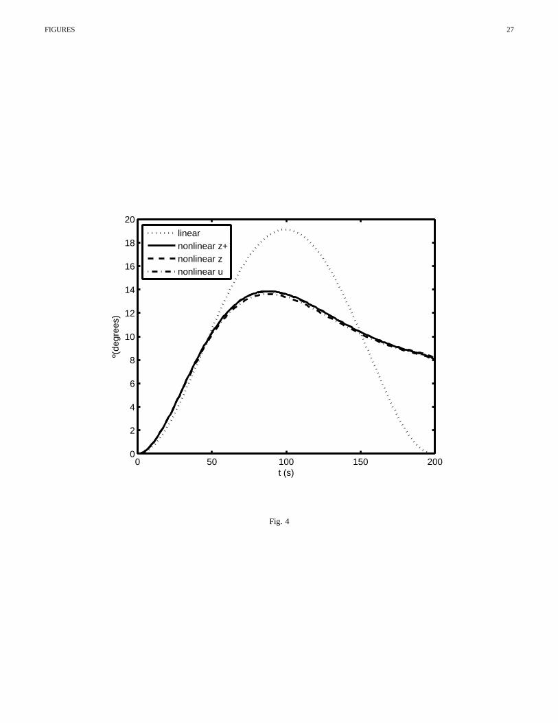
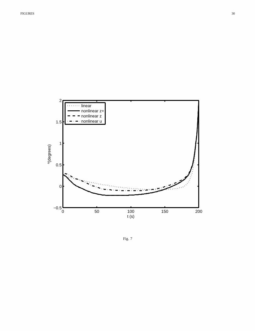
As shown in Figs. 3, 4, 6 and 7 continuous, dash/dot and dashedlines are essentially the same. However,

there is some differences between them in Figs. 2 and 5. Obviously, the reason for these results is that

in nonlinear z+and innonlinear uwe force the submarine to finish near to zero position on they−axis,

but in nonlinear uwe also constrain the movement of the rudderδr which gives the movement on the

y−axis. Therefore,δr needs to turn more innonlinear z+ than in nonlinear u, where this movement is

restrictive, or innonlinear z, where the constraint ony−axis is inactive. It is in Figs. 2 and 5 where we

can see clearly the effect of coupling, since in the linear model there is no change on they−axis and no

movement of the rudderδr is needed, but in the nonlinear coupled model the variation on y−axis is very

notorious and movements of rudder are needed to correct thatvariation.

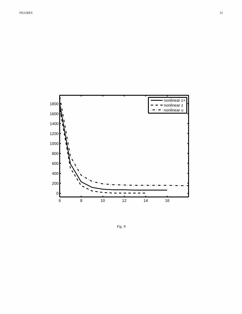
Finally, Fig. 8 shows the evolution of the cost function (with respect to the number of iterations) for

the casesnonlinear z, nonlinear z+ and nonlinear u. An exponential decay is observed in all cases.

As expected, the minimal cost is reached for the less restrictive problemnonlinear zin less number of

iterations, and the largest cost is reached for the more restrictive problemnonlinear uin a larger number

of iterations. We do not include pictures for the rest of state variables because they are not relevant in

this manoeuvre.

As is typical in a gradient algorithm, results depend on the initialization. For instance, when we initiate

our algorithm with zero value foru (t) , 0 ≤ t ≤ tf , after convergence, we obtain different results: the

costs for the casenonlinear zare the same and very close to zero, but the optimal controls are slightly

18

different; for the casenonlinear z+,the final optimal cost is higher than in the case tested before, and the

optimal controls are also different. These results seem to indicate the existence of several local minima

and/or non-uniqueness of solutions.

B. Turning manoeuvre

We simulate a turning manoeuvre for a constant deflection of rudder of−20o and an average surge

velocity of 7.5 m/s. This is a typical test of amanoeuvre in a complex scenario. The aim we pursue is

precision in turning manoeuvre and, at the same time, a minimum change in vertical displacement.

In order to achieve that goal, we modify slightly the parameters Φ and F in the cost function, as

follows:

Φ(x (tf ) ,x

tf

)= 0 (25)

and

F (x (t) ,u (t)) =3∑

j=1

βj (uj (t))2 +12∑

j=1

ϑi (xi (t))2 (26)

with δi > 0 weight parameters. Now, the cost function is a commitment between a minimal expense of

control on having done the corresponding manoeuvre and a minimal change on the state variables. For

the turning test, particulary we desire the vertical displacement to be the minimum possible. Since this

type of manoeuvre is not very usual, we do not worry about optimization with respect to controls energy.

Therefore, we take:

λ = 0.01 ε = 10−6

ϑ3 = 1, ϑi = 0, i 6= 3,

βj = 0, j = 1, 2, 3

x (0) = (0, 0, 0, 0, 0, 90, 7.5, 0, 0, 0, 0,−1.5)

tf = 400s.

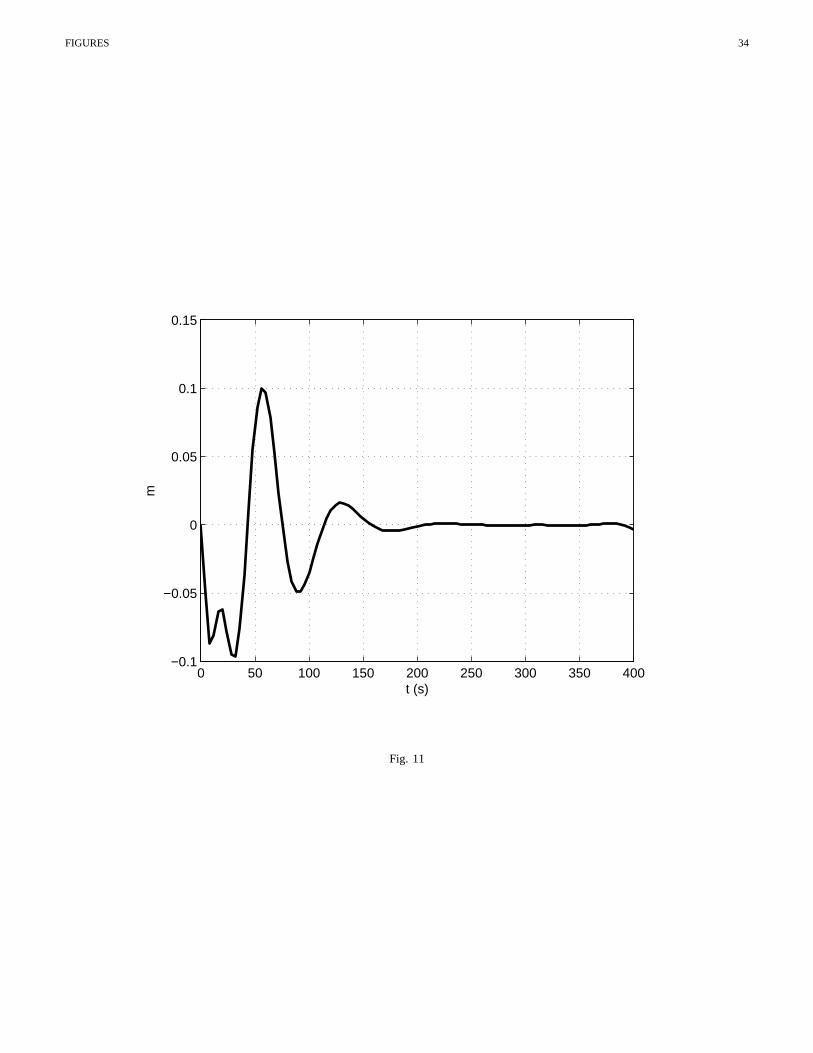
Results are displayed in Figs. 9-18. As shown by these pictures, the turning manoeuvre is very accurate,

while the vertical displacement is very small. Fig. 9 displays the three-dimensional turning movement. It

19

reaches a minimum on thez−axis of−0.1m and a peak of0.1m, which compared to the initial movement

with δs = 1o and δb = −0.9o during the entire simulation time, where the minimum is−1.6m and the

maximum is1.4m, presents a reduction about90% on the vertical displacement, and compared to the

manoeuvre without moving stern and bow planes (the uncoupled case) where the minimum is−45m and

the maximum is0m, the reduction is about99%. In this manoeuvre, it is also clear the coupling effect,

since in a decoupled model there are no variations on the depth variable,z, there is no need to move

stern and bow planes. But, for our model the initial variationwas about45m and to correct that, it was

necessary to move both, stern and bow planes, because such a variation could cause a collision where

moving in littoral scenarios.

VI. CONCLUSION

Numerical results obtained from the optimization method proposed show that the coupling effects

inherent to the highly nonlinear and coupled mathematical model for the specific named submarine model

considered in this work are not negligible. Of course, theseeffects can not be detected with linear

or uncoupled nonlinear models. In this respect, it is interesting to point out that International Marine

Organization (IMO) accepts results obtained from numerical simulation for ships models validation. Up

to knowledge of the authors, for the moment, the case of underwater vehicles has not been received IMO’s

attention, but it could be the case in the near future. The present work may therefore be useful in this

sense. However, the main applications of the results of thiswork are:

• Assist designers during the preliminary state design of thesubmarine. For instance, the parameters

for position and shape of the control surfaces appear in the hydrodynamic coefficients and these

affect the manoeuvrability capability of the underwater vehicle, which can be simulated with the

model considered in this work. Therefore, designers can adapt those design parameters to obtain and

specific and desired submarine’s dynamics.

• As a guidance system since the approach of this work providesa set of manoeuvres which are

admissible for our specific model. These manoeuvres are the starting point for the design of controllers

20

based on feedback laws.

In what concerns the computational cost of the gradient algorithm proposed, in terms of computer time

consuming and for a PC with 2.66 GHz and 2 GB RAM memory, dept change manoeuvres tested take

about 50 seconds. However, the turning manoeuvre simulatedrequires about 1 hour. For the purposes of

the present work, computational cost is not an essential issue. Our main goal was to analyze coupling

effects in the nonlinear mathematical model and to do so withrigorous mathematics. We emphasize that

discontinuities in an ODE system (which in our case appear inthe adjoint state law) may be a very

delicate issue in the numerical computation of its solution.

As for possible extensions of the results in this work, we would like to mention:

(a) Consider more general costs involving explicitly a quadratic dependance on the derivatives of

control variables. This issue is of a major importance in minimizing noise generation.

(b) Consider also explicitly constraints on both control, variables and the rate at which they change.

(c) Include propeller revolution as a control variable.

(d) Study the minimum time problem associated with our model.

We plan to analyze these matters in a future work.

APPENDIX

Table of Parameters

ACKNOWLEDGEMENT

The authors would like to thank Professor Thor I. Fossen for his time, the stimulating conversations

about this work and the advices given.

REFERENCES

[1] Underwater Vehicles, Edited by A. V. Inzartsev, I-Tech Educationand Publishing, 2009.

[2] A. J. Healey and D. Lienard, Multivariable sliding-mode control forautonomous diving and steering of unmanned vehicles, IEEE

Journal of Oceanic Engineering 18 (3) (1993), 327-339.

21

[3] J. Felman, Revised standard submarine equations of motion. Report DTNSRDC/SPD-0393-09, David W. Taylor Naval Ship Research

and Development Center, Washington D.C., 1979.

[4] E. Bφrhaug, A. Pavlov and K. Y. Pettersen, Straight Line Path Following for Formations of Underactuated Underwater Vehicles,

Proceedings of the 46th IEEE Conference on Decision and Control NewOrleans, 2007.

[5] K. Y. Pettersen and T. I. Fossen, Underactuated Dynamic Positioning of a Ship - Experimental Results, IEEE Transactions On Control

Systems Technology, 2000.

[6] J. Silva and J. Sousa, Models for Simulation and Control of Underwater Vehicles, New Approaches in Automation and Robotics, Edited

by H. Aschemann, I-Tech Education and Publishing, 2008.

[7] T. I. Fossen, Guidance and control of ocean vehicles, John Wileyand sons, 1994.

[8] M. Gertler and G. R. Hagen, Standard equations of motionfor submarine simulations, NSRDC Rep. 2510, 1967.

[9] J. N. Newman, Marine hydrodynamics, The MIT Press, Cambridge, Massachusetts, London, 1977.

[10] A. F. Filippov, Differential equations with discontinuous right-hand side, Mat. Sb. (N.S.) 51 (93), 99-128 (1960) [in Russian]. Engl.

Transl.: AMS Translations, Series 2, Vol. 42, pp. 199-231 (1964).

[11] T. I. Fossen, Marine Control Systems: Guidance, Navigation andControl of Ships, Rigs and Underwater Vehicles, Marine Cybernetics

AS, Trondheim, 2002.

[12] J. Garcıa-Pelaez, J. A. Murillo, I. A. Nieto, D. Pardo and F. Periago, Numerical simulation of a depth controller for an underwater

vehicle, MARTECH’07, International Workshop on Marine Technology, Villanova i la Geltru, 2007.

[13] K. Ogata, Modern Control Engineering. Prentice-Hall, fourth edition edition, 2001.

[14] J. C. Culioli, Introductiona l’optimisation,Editions Ellipses, Paris 1994.

[15] H. Hairer, S. P. Nφrsett and G. Wanner, Solving Ordinary Differential Equations I. Non stiff problems, Second revised edition, Springer

series in computational mathematics, 2000.

[16] R. Mannshardt, One-step methods for any order ordinary differential equations with discontinuous right-hand sides, Numer. Math. 31

(1978), 131-152.

[17] L. F. Shampine, M. W. Reichelt, The Matlab ODE Suit. SIAM Journal on Scientific Computing, vol. 18, 1997, pp 1-22.

22

Javier Garcıa is Naval Architect and Marine Engineer for the Polytechnic University ofMadrid, Spain. He holds

in Navantia the current position of Cartagena Engineering Delegation General Design Manager. In particular, he is

responsible for Hydrodynamics and Signatures Management of the Submarine Projects for this company.

Diana Ovalle received the Engineering degree in electronics in 2005 from the Distrital University of Colombia. She

obtained her Ms.C. degree in electric engineering in 2007 from the University of the Andes, in Colombia.

From 2008, she is a Ph.D. student at the Department of Applied Mathematics and Statistics of the Polytechnic University

of Cartagena, Spain. Her main scientific interests are in nonlinear controlsystems and numerical simulation, theoretical

and industrial applications.

Francisco Periagois an Assistant Professor at the Department of Applied Mathematics and Statistics of the Polytechnic

University of Cartagena, Spain. He obtained his Ph.D. in applied mathematics in 1999 at the University of Valencia,

Spain. His main research interest includes Optimal Control, Optimal Designand Controllability, both at the theoretical

level and its application to industrial problems. At present, he is responsible for the research projects 2113/07MAE,

in collaboration with the company NAVANTIA S.A., and 08720/PI/08 from Fundacion Seneca (Region de Murcia,

Spain).

23

L IST OF FIGURES

1 Appearance of the model studied in this work. . . . . . . . . . . . .. . . . . . . . . . . . . 24

2 East movement,y(t) . . . . . . . . . . . . . . . . . . . . . . . . . . . . . . . . . . . . . . . . 25

3 Depth movement,z(t) . . . . . . . . . . . . . . . . . . . . . . . . . . . . . . . . . . . . . . . 26

4 Pitch Angle,θ(t) . . . . . . . . . . . . . . . . . . . . . . . . . . . . . . . . . . . . . . . . . 27

5 Deflection of rudder,δr(t) . . . . . . . . . . . . . . . . . . . . . . . . . . . . . . . . . . . . . 28

6 Deflection of stern plane,δs(t) . . . . . . . . . . . . . . . . . . . . . . . . . . . . . . . . . . 29

7 Deflection of bow plane,δb(t) . . . . . . . . . . . . . . . . . . . . . . . . . . . . . . . . . . 30

8 Cost Function . . . . . . . . . . . . . . . . . . . . . . . . . . . . . . . . . . . . . . .. . . . 31

9 Three-dimensional movement . . . . . . . . . . . . . . . . . . . . . . . . .. . . . . . . . . . 32

10 Movement x-y plane . . . . . . . . . . . . . . . . . . . . . . . . . . . . . . . . .. . . . . . 33

11 Depth movement,z(t) . . . . . . . . . . . . . . . . . . . . . . . . . . . . . . . . . . . . . . . 34

12 Roll angle,φ(t) . . . . . . . . . . . . . . . . . . . . . . . . . . . . . . . . . . . . . . . . . . 35

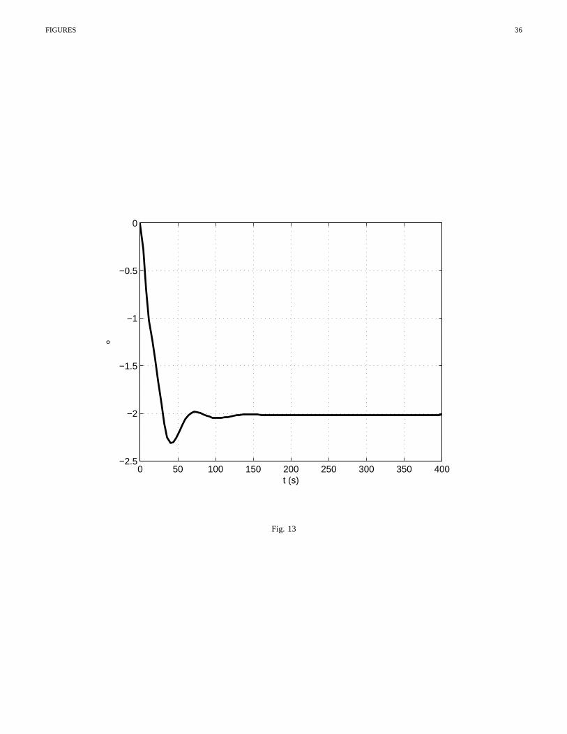
13 Pitch angle,θ(t) . . . . . . . . . . . . . . . . . . . . . . . . . . . . . . . . . . . . . . . . . . 36

14 Yaw angle,ψ(t) . . . . . . . . . . . . . . . . . . . . . . . . . . . . . . . . . . . . . . . . . . 37

15 Deflection of rudder,δr(t) . . . . . . . . . . . . . . . . . . . . . . . . . . . . . . . . . . . . 38

16 Deflection of stern plane,δs(t) . . . . . . . . . . . . . . . . . . . . . . . . . . . . . . . . . . 39

17 Deflection of bow plane,δb(t) . . . . . . . . . . . . . . . . . . . . . . . . . . . . . . . . . . 40

18 Cost function . . . . . . . . . . . . . . . . . . . . . . . . . . . . . . . . . . . . . .. . . . . 41

FIGURES 24

Fig. 1

FIGURES 25

0 50 100 150 200−8

−7

−6

−5

−4

−3

−2

−1

0

1

t (s)

m

linearnonlinear z+nonlinear znonlinear u

Fig. 2

FIGURES 26

0 50 100 150 2000

50

100

150

200

250

300

350

400

450

t (s)

m

linearnonlinear z+nonlinear znonlinear u

Fig. 3

FIGURES 27

0 50 100 150 2000

2

4

6

8

10

12

14

16

18

20

t (s)

º(de

gree

s)

linearnonlinear z+nonlinear znonlinear u

Fig. 4

FIGURES 28

0 50 100 150 200−0.12

−0.1

−0.08

−0.06

−0.04

−0.02

0

0.02

t (s)

º(de

gree

s)

linearnonlinear z+nonlinear znonlinear u

Fig. 5

FIGURES 29

0 50 100 150 200−4

−3.5

−3

−2.5

−2

−1.5

−1

−0.5

0

0.5

1

t (s)

º(de

gree

s)

linearnonlinear z+nonlinear znonlinear u

Fig. 6

FIGURES 30

0 50 100 150 200−0.5

0

0.5

1

1.5

2

t (s)

º(de

gree

s)

linearnonlinear z+nonlinear znonlinear u

Fig. 7

FIGURES 31

6 8 10 12 14 16

0

200

400

600

800

1000

1200

1400

1600

1800

nonlinear z+nonlinear znonlinear u

Fig. 8

FIGURES 32

−500

50100

150200

−300

−200

−100

0−0.1

−0.05

0

0.05

0.1

0.15

x(m)y(m)

z(m

)

Fig. 9

FIGURES 33

−50 0 50 100 150 200−250

−200

−150

−100

−50

0

x(m)

y(m

)

Fig. 10

FIGURES 34

0 50 100 150 200 250 300 350 400−0.1

−0.05

0

0.05

0.1

0.15

t (s)

m

Fig. 11

FIGURES 35

0 50 100 150 200 250 300 350 400−14

−12

−10

−8

−6

−4

−2

0

t (s)

º

Fig. 12

FIGURES 36

0 50 100 150 200 250 300 350 400−2.5

−2

−1.5

−1

−0.5

0

t (s)

º

Fig. 13

FIGURES 37

0 50 100 150 200 250 300 350 400−1200

−1000

−800

−600

−400

−200

0

t (s)

º

Fig. 14

FIGURES 38

0 50 100 150 200 250 300 350 40019

19.2

19.4

19.6

19.8

20

20.2

20.4

20.6

20.8

21

t (s)

º

Fig. 15

FIGURES 39

0 50 100 150 200 250 300 350 4000

0.5

1

1.5

2

2.5

3

t (s)

º

Fig. 16

FIGURES 40

0 50 100 150 200 250 300 350 400−2

−1.8

−1.6

−1.4

−1.2

−1

−0.8

−0.6

−0.4

−0.2

0

t (s)

º

Fig. 17

FIGURES 41

0 500 1000 1500

0.01

0.02

0.03

0.04

0.05

0.06

0.07

0.08

0.09

0.1

0.11

# of iterations

cost

Fig. 18

FIGURES 42

L IST OF TABLES

I Linear Hydrodynamic Coefficients . . . . . . . . . . . . . . . . . . . . . .. . . . . . . . . . 43

II Nonlinear Hydrodynamic Coefficients . . . . . . . . . . . . . . . . . .. . . . . . . . . . . . 44

TABLES 43

TABLE I

m′= 1.71e − 02 Y ′

v = −1.80e − 02 Y ′r = −8.30e − 04

L = 60 N ′v = 6.80e − 04 kzz = 0.849

N ′r = −8.14e − 04 Z′

w = −1.46e − 02 Z′q = −7.00e − 05

M ′w = −1.40e − 03 kyy = 1.047 M ′

q = −6.37e − 04

Y ′v = 0 u0 = 8 Y ′

r = 0

N ′v = −2.30e − 02 N ′

r = 0 Z′w = 0

Z′q = 0 M ′

w = 6.26e − 03 M ′q = 0

ρ = 1000 Zg = 0.089 W = 435

Zb = 0 B = 435

Y ′δr

= 9.03e − 03 N ′δr

= −4.06e − 03 Z′δs

= −6.25e − 03

M ′δs

= −2.45e − 03 Z′δb

= −3.19e − 03 M ′δb

= 6.38e − 04

TABLES 44

TABLE II

m = 2352 l = 67 XG = 0

YG = 0 ZG = −0.356 ρ = 1.026

X ′u = −0.00046 Y ′

v = −0.06136 N ′v = 0.00068

Z′w = −0.0144 M ′

w = −0.00139 K′p = −0.00007

N ′p = −0.00003 Z′

q = −0.00007 M ′q = −0.00098

K′v = −0.0006 Y ′

p = −0.0003 Ix = 16390

Iy = 659770 Iz = 659770 Ixy = 0

Izx = 0 Iyz = 0

X ′uu = −0.0011 X ′

vv = 0.01746 X ′ww = 0.00775

X ′rp = 0.0006 X ′

qq = 0.00142 X ′q|q| = 0

X ′rr = 0.00208 X ′

vr = 0.0224 Y ′∗ = 0

Y ′v = −0.06137 Y ′

v|v| = −0.02814 Y ′p = −0.00305

Y ′wp = 0.0144 Y ′

pq = 0.00007 Y ′r|r| = 0.00465

Y ′r = 0.0007 Z′

∗ = −0.0003 Z′|w| = −0.002

Z′vv = 0.185 Z′

w = −0.02028 Z′ww = 0.02

Z′vp = −0.01837 Z′

q|q| = −0.00398 Z′q = −0.00699

Z′rr = −0.00396 Z′

vr = −0.04513 M ′∗ = 0.00002

M ′|w| = −0.00036 M ′

vv = 0.03461 M ′w = 0.00478

M ′ww = 0.00045 M ′

rp = 0.00112 M ′q|q| = −0.00303

M ′q = −0.00389 M ′

rr = −0.00119 M ′vr = −0.01573

K′∗ = 0 K′

v = −0.00287 K′v|v| = −0.00214

K′p|p| = −0.0003 K′

wp = −0.00021 K′p = −0.00062

K′qr = 0.0003 K′

r|r| = −0.00019 K′r = 0.00026

N ′∗ = 0 N ′

v = −0.01864 N ′v|v| = 0.01868

N ′p = −0.00068 N ′

pq = −0.00091 N ′r|r| = 0.00209

N ′r = −0.00483 X ′

w|w| = 0 X ′wq = −0.01316

M ′vw = 0

Y ′δr

= −0.00083 K′δr

= −0.00005 N ′δr

= −0.0012

X ′δrδr

= −0.0039 X ′δsδs

= −0.00119 X ′δbδb

= −0.00299

Y ′δr

= −0.00083 Y ′δrη = 0.00067 Z′

δs= −0.00512

Z′δsη = −0.00045 Z′

δb= −0.00512 K′

δr= −0.00005

M ′δs

= −0.00231 M ′δsη = −0.00038 M ′

δb= 0.00094

N ′δr

= −0.0012 N ′δrη = −0.00034 XB = 0

YB = 0 ZB = −0.621 B = 23073.1

W = 23073.1 n = 2

KT0 = 0.525403 KTJ = −0.338313 KTJ2 = −0.197236

KTJ3 = 0 KTJ4 = 0 η = 1.09431

C = 0.8976 KQ0 = 0.070405 KQJ = −0.02846

KQJ2 = −0.033684 KQJ3 = 0 KQJ4 = 0

t = 0.344 wf = 0.148 D = 3.821

Y ′vwN = −0.303 Y ′

v|v|N = −0.1162 Z′w|w|R = 0.0077

N ′vwN = −0.303 M ′

w|w|N = −0.00674 N ′v|v|N = −0.0185